Download fulltext - DiVA Portal

Tracking objects with fixed-wing UAV
using model predictive control and
machine vision
Stian Aas Nundal
Espen Skjong
Master of Science in Cybernetics and Robotics
Submission date: June 2014
Supervisor:
Tor Arne Johansen, ITK
Norwegian University of Science and Technology
Department of Engineering Cybernetics
NORWEGIAN UNIVERSITY OF SCIENCE AND TECHNOLOGY
Faculty of Information Technology, Mathematics and Electrical Engineering
Department of Engineering Cybernetics
MASTER THESIS
For the Degree of MSc Engineering Cybernetics
Tracking objects with fixed-wing UAV using model predictive control and
machine vision
Supervisor:
Authors:
Professor Tor Arne Johansen
Espen Skjong
Stian Aas Nundal
Department of Engineering Cybernetics
Centre for Autonomous Marine Operations and
Systems
Department of Engineering Cybernetics
Co-supervisors:
Ph.D. Candidate
Frederik Stendahl Leira
Department of Engineering Cybernetics
Centre for Autonomous Marine Operations and
Systems
Professor Thor Inge Fossen
Department of Engineering Cybernetics
Centre for Autonomous Marine Operations and
Systems
Trondheim, June 2, 2014
Abstract
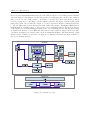
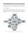
This thesis describes the development of an object tracking system for unmanned aerial vehicles
(UAVs), intended to be used for search and rescue (SAR) missions. The UAV is equipped
with a two-axis gimbal system, which houses an infrared (IR) camera used to detect and track
objects of interest, and a lower level autopilot. An external computer vision (CV) module is
assumed implemented and connected to the object tracking system, providing object positions
and velocities to the control system. The realization of the object tracking system includes
the design and assembly of the UAV’s payload, the design and implementation of a model
predictive controller (MPC), embedded in a larger control environment, and the design and
implementation of a human machine interface (HMI). The HMI allows remote control of the
object tracking system from a ground control station. A toolkit for realizing optimal control
problems (OCP), MPC and moving horizon estimators (MHE), called ACADO, is used. To gain
real-time communication between all system modules, an asynchronous multi-threaded running
environment, with interface to external HMIs, the CV module, the autopilot and external control
systems, was implemented. In addition to the IR camera, a color still camera is mounted in the
payload, intended for capturing high definition images of objects of interest and relaying the
images to the operator on the ground. By using the center of the IR camera image projected
down on earth, together with the UAV’s and the objects’ positions, the MPC is used to calculate
way-points, path planning for the UAV, and gimbal attitude, which are used as control actions
to the autopilot and the gimbal. Communication between the control system and the autopilot
is handled by DUNE. If multiple objects are located and are to be tracked, the control system
utilizes an object selection algorithm that determines which object to track depending on the
distance between the UAV and each object. If multiple objects are clustered together, the object
selection algorithm can choose to track all the clustered objects simultaneously. The object
selection algorithm features dynamic object clustering, which is capable of tracking multiple
moving objects. The system was tested in simulations, where suitable ACADO parameters
were found through experimentation. Important requirements for the ACADO parameters
are smooth gimbal control, an efficient UAV path and acceptable time consumption. The
implemented HMI gives the operator access to live camera streams, the ability to alter system
parameters and manually control the gimbal. The object tracking system was tested using
hardware-in-loop (HIL) testing, and the results were encouraging. During the first flight of
the UAV, without the payload on-board, the UAV platform exhibited erroneous behaviour and
the UAV was grounded. A solution to the problem was not found in time to conduct any
further flight tests during this thesis. A prototype for a three-axis stabilized brushless gimbal
was designed and 3D printed. This was as a result of the two-axis gimbal system’s limited
stabilization capabilities, small range of movement and seemingly fragile construction. Out of
a suspected need for damping to improve image quality from the still camera, the process of
designing and prototyping a wire vibration isolator camera mount was started. Further work
and testing is required to realize both the gimbal and dampened camera mount. The lack of
flight tests prohibited the completion of the object tracking system.
Keywords: object tracking system, unmanned aerial vehicle (UAV), search and rescue,
two-axis gimbal system, infrared (IR) camera, computer vision (CV), model predictive
control (MPC), control environment, human machine interface (HMI), remote control, ground
control, ACADO, real-time, asynchronous multi-threaded running environment, way-point, path
planning, DUNE, dynamic object clustering, multiple moving objects, hardware-in-loop (HIL),
three-axis stabilized brushless gimbal, wire vibration isolator
Samandrag
Denne avhandlinga tek føre seg utviklinga av eit system for å overvake og spore objekt
av interesse i samanheng med redningsoppdrag. Systemet vart utvikla som ei modelær
nyttelast for ei eksisterande ubemanna, sjølvstyrt flyplattform, kjent som UAV eller drone.
Nyttelasta er utstyrt med eit infraraudt (IR) kamera, montert i ein stabilisert toaksa gimbal,
som brukast til å detektere og overvake objekta. Til denne avhandlinga er det antatt at
ein maskinsynmodul allereie er implementert, og i stand til å forsyne styringssystemet med
posisjon- og rørsledata frå objekta. Realiseringa av systemet inneber planlegging og bygging av
nyttelasta, planlegging, utgreiing og implementasjon av ein modell-prediktiv regulator (MPC)
som del av eit større styringsmiljø, samt utvikling og implementasjon av eit brukargrensesnitt
(HMI). Brukargrensesnittet tillèt fjernstyring av systemet frå kontrollstasjonen på bakken. Til
implementasjonen av MPC vart det nytta eit programmeringsbibliotek, kalla ACADO, som
brukast til å løyse optimaliseringsproblem. For å oppnå sanntidskommunikasjon mellom dei
forskjellige modulane i systemet, vart det utvikla og implementert eit asynkront fleirtråda miljø
der brukargrensesnittet, CV modulen, autopiloten og styringssystemet snakkar saman. I tillegg
til IR kameraet er det montert eit fargekamera i nyttelasta, som skal gi operatøren på bakken
tilgang til høgoppløyste bilete av objekta i sanntid. Ved å gjere nytte av kjend informasjon om
flyet sin posisjon og åtferd, saman med objekta sine posisjonar og rørsler, er styringssystemet
i stand til å berekne ei effektiv rute, som blir formidla til autopiloten i form av etappepunkt.
Systemet bereknar òg vinklar til gimbalen slik at kameraet alltid skal vere retta mot det målet
som til ei kvar tid vert overvaka. Kommunikasjonen mellom styringssystemet og autopiloten vert
handtert av DUNE. I situasjonar der fleire objekt skal overvakast samstundes nyttar systemet
seg av ei algoritme som planlegg ruta mellom dei forskjellige objekta ved å til ei kvar tid gå
til det næraste uvitja objektet. Når alle objekta har vore vitja i inneverande sløyfe, vert lista
nullstilt og algoritma byrjar på nytt ved det fyrste objektet. Dersom nokon av objekta finn seg
nær kvarandre kan det vere hensiktsmessig å sjå dei som eit objekt. Dette løyser algoritma ved
å dynamisk legge objekta til eller ta dei ut or gruppe, etter som objekta bevegar seg mot eller
frå kvarandre, der alle objekta i ei gruppe skal overvakast saman. Systemet vart grundig testa
gjennom simuleringar, der variablar for ACADO vart utarbeidd. For å finne gode variablar
vart det lagt vekt på følgjande kriteria: Jamne gimbalrørsler, effektiv flyrute og akseptabel
tidsbruk. Brukargrensesnittet gjev operatøren tilgang til direkte straumar frå begge kamera,
høve til å forandre systemvariablar samt å manuelt styre vinklane til gimbalen. Systemet
vart òg testa på laben, gjennom hardware-in-loop (HIL) testar, der det viste tilfredsstillande
eigenskapar. Systemet vart ikkje testa i lufta, då problem med flyplatforma forhindra flyging
med nyttelasta utvikla i denne avhandlinga. Feilen vart diverre ikkje retta i tide til leveringa av
denne avhandlinga. På grunn av manglande stabiliseringseigenskapar, avgrensa arbeidsområde
og den tilsynelatande skjøre konstruksjon til den toaksa gimbalen, vart det utvikla ein prototype
for ein treaksa gimbal som nyttar kostelause motorar. Det vart òg eksperimentert med å bruke
wire til å dempe vibrasjonar i innfatninga til fargekameraet. Det er behov for meir testing for
å ferdigstille både gimbalen og det dempa kamerafestet. Mangelen på flytid gjorde at systemet
ikkje kunne ferdigstillast innanfor dei gitte tidsrammene til denne avhandlinga.
Preface
The present thesis is submitted in partial fulfillment of the requirements for the degree MSc.
at the Norwegian University of Science and Technology.
The thesis is based on our research last semester, which was submitted in December 2013
(Skjong and Nundal, 2013).
The thesis has involved many different aspects, both practical and theoretical. First of all we
would like to thank Professor Tor Arne Johansen for his guidance, support and encouragement.
He has given us many valuable ideas in which have formed this thesis. We would also thank
Ph.D. candidate Frederik Stendahl Leira for his outstanding cooperation in both interfacing
the CV module and realizing the total object tracking system. Also Professor Thor Inge Fossen
deserves a thank for giving us interesting points of view outlining possible system solutions.
Without pilots, no tests could have been conducted. We therefore want to thank the pilots,
Lars Semb and Carl Erik Stephansen, for their expertise in maintaining and piloting the UAV,
and for taking interest in our research. We are disappointed for not being able to conduct any
flight tests, but this is not from the pilots’ lack of effort.
The guys at the institute’s mechanical workshop, Per Inge Snildal and Terje Haugen, deserves
a thank for their experience and contribution when prototyping all mechanical parts of the
UAV’s payload.
Finally, we would like to thank our parents for their support.
Trondheim, June 24, 2014.
Espen Skjong
Stian Aas Nundal
iii
"We are entering an era in which unmanned vehicles of all
kinds will take on greater importance in space, on land, in
the air, and at sea (2001)."
- President George W. Bush,
Address to the Citadel
Contents
List of Figures
xiii
List of Tables
xix
Nomenclature
xxiii
1 Introduction
1.1 A historical view: The UAV’s development . . . . . . . . . . . . . . . . . . . . .
1.2 Background . . . . . . . . . . . . . . . . . . . . . . . . . . . . . . . . . . . . . . .
1.3 Thesis outline . . . . . . . . . . . . . . . . . . . . . . . . . . . . . . . . . . . . . .
1
1
1
3
2 Computer vision
2.1 Introduction to computer vision . . . . . . . . . . . . . . . . . . . . . . . . . . . .
2.2 CV and UAV’s . . . . . . . . . . . . . . . . . . . . . . . . . . . . . . . . . . . . .
2.3 Pre-implemented CV module . . . . . . . . . . . . . . . . . . . . . . . . . . . . .
7
7
8
9
3 UAV dynamics
3.1 Coordinate frames and positions . . . . . . . . . . . . . . . . . . . . . . . . .
3.1.1 The UAV’s position relative earth . . . . . . . . . . . . . . . . . . . .
3.1.2 The gimbal’s position relative earth . . . . . . . . . . . . . . . . . . .
3.1.3 Pan and tilt angles relative body frame . . . . . . . . . . . . . . . . .
3.1.4 Camera lens position relative the gimbal’s center . . . . . . . . . . . .
3.2 Geographic coordinate transformations . . . . . . . . . . . . . . . . . . . . . .
3.2.1 Transformation between geographic coordinates and the ECEF frame
3.2.2 Transformation between the ECEF frame and a local ENU frame . . .
3.3 Kinematics . . . . . . . . . . . . . . . . . . . . . . . . . . . . . . . . . . . . .
3.4 Bank angle . . . . . . . . . . . . . . . . . . . . . . . . . . . . . . . . . . . . .
.
.
.
.
.
.
.
.
.
.
.
.
.
.
.
.
.
.
.
.
11
11
13
14
14
16
16
18
20
21
22
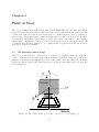
4 Field of View
25
4.1 The projected camera image . . . . . . . . . . . . . . . . . . . . . . . . . . . . . . 25
4.2 Projected camera image constraints . . . . . . . . . . . . . . . . . . . . . . . . . . 29
5 Model Predictive Control
5.1 Background . . . . . . . .
5.2 Gimbal attitude . . . . . .
5.3 UAV attitude . . . . . . .
5.4 Moving objects . . . . . .
5.5 Objective function . . . .
5.6 Tracking multiple objects
5.7 System description . . . .
.
.
.
.
.
.
.
.
.
.
.
.
.
.
.
.
.
.
.
.
.
.
.
.
.
.
.
.
.
.
.
.
.
.
.
.
.
.
.
.
.
.
.
.
.
.
.
.
.
vii
.
.
.
.
.
.
.
.
.
.
.
.
.
.
.
.
.
.
.
.
.
.
.
.
.
.
.
.
.
.
.
.
.
.
.
.
.
.
.
.
.
.
.
.
.
.
.
.
.
.
.
.
.
.
.
.
.
.
.
.
.
.
.
.
.
.
.
.
.
.
.
.
.
.
.
.
.
.
.
.
.
.
.
.
.
.
.
.
.
.
.
.
.
.
.
.
.
.
.
.
.
.
.
.
.
.
.
.
.
.
.
.
.
.
.
.
.
.
.
.
.
.
.
.
.
.
.
.
.
.
.
.
.
.
.
.
.
.
.
.
.
.
.
.
.
.
.
.
.
.
.
.
.
.
.
.
.
.
.
.
.
.
.
.
.
.
.
.
33
33
35
38
38
39
40
44
viii
Contents
5.8
5.9
ACADO - implementation aspects
Additional system improvements .
5.9.1 Feed forward gimbal control
5.9.2 Closed loop feedback . . . .
5.9.3 Improved objective function
5.9.4 Input blocking . . . . . . .
.
.
.
.
.
.
.
.
.
.
.
.
.
.
.
.
.
.
.
.
.
.
.
.
.
.
.
.
.
.
.
.
.
.
.
.
.
.
.
.
.
.
.
.
.
.
.
.
.
.
.
.
.
.
.
.
.
.
.
.
.
.
.
.
.
.
.
.
.
.
.
.
.
.
.
.
.
.
.
.
.
.
.
.
.
.
.
.
.
.
.
.
.
.
.
.
.
.
.
.
.
.
.
.
.
.
.
.
.
.
.
.
.
.
.
.
.
.
.
.
.
.
.
.
.
.
.
.
.
.
.
.
.
.
.
.
.
.
.
.
.
.
.
.
.
.
.
.
.
.
.
.
.
.
.
.
45
45
46
46
47
47
6 Control system design
6.1 Hardware and interfaces . . . . . . . . . . . . . .
6.2 Introducing UML . . . . . . . . . . . . . . . . . .
6.3 Overview of the control objective . . . . . . . . .
6.4 General control system architecture . . . . . . . .
6.5 Synchronous and asynchronous threading . . . .
6.6 System architecture . . . . . . . . . . . . . . . .
6.6.1 MPC engine . . . . . . . . . . . . . . . . .
6.6.2 Piccolo threads . . . . . . . . . . . . . . .
6.6.3 CV threads . . . . . . . . . . . . . . . . .
6.6.4 HMI threads . . . . . . . . . . . . . . . .
6.6.5 External control system interface threads
6.7 Supervision of control inputs . . . . . . . . . . .
6.8 System redundancy . . . . . . . . . . . . . . . . .
6.8.1 Software redundancy . . . . . . . . . . . .
6.8.2 Hardware redundancy . . . . . . . . . . .
6.9 Signal dropouts . . . . . . . . . . . . . . . . . . .
6.10 System configuration . . . . . . . . . . . . . . . .
6.11 Logging and debugging . . . . . . . . . . . . . . .
6.12 Implementation aspects . . . . . . . . . . . . . .
.
.
.
.
.
.
.
.
.
.
.
.
.
.
.
.
.
.
.
.
.
.
.
.
.
.
.
.
.
.
.
.
.
.
.
.
.
.
.
.
.
.
.
.
.
.
.
.
.
.
.
.
.
.
.
.
.
.
.
.
.
.
.
.
.
.
.
.
.
.
.
.
.
.
.
.
.
.
.
.
.
.
.
.
.
.
.
.
.
.
.
.
.
.
.
.
.
.
.
.
.
.
.
.
.
.
.
.
.
.
.
.
.
.
.
.
.
.
.
.
.
.
.
.
.
.
.
.
.
.
.
.
.
.
.
.
.
.
.
.
.
.
.
.
.
.
.
.
.
.
.
.
.
.
.
.
.
.
.
.
.
.
.
.
.
.
.
.
.
.
.
.
.
.
.
.
.
.
.
.
.
.
.
.
.
.
.
.
.
.
.
.
.
.
.
.
.
.
.
.
.
.
.
.
.
.
.
.
.
.
.
.
.
.
.
.
.
.
.
.
.
.
.
.
.
.
.
.
.
.
.
.
.
.
.
.
.
.
.
.
.
.
.
.
.
.
.
.
.
.
.
.
.
.
.
.
.
.
.
.
.
.
.
.
.
.
.
.
.
.
.
.
.
.
.
.
.
.
.
.
.
.
.
.
.
.
.
.
.
.
.
.
.
.
.
.
.
.
.
.
.
.
.
.
.
.
.
.
.
.
.
.
.
.
.
.
.
.
.
.
.
.
.
.
.
.
.
.
.
.
.
.
.
.
.
.
.
.
.
.
.
.
49
49
52
52
54
56
58
59
61
63
64
66
67
67
68
68
69
70
71
71
7 HMI - Human Machine Interface
7.1 Qt and qml . . . . . . . . . . . . . . . . . . . . . .
7.2 HMI requirements . . . . . . . . . . . . . . . . . .
7.3 System architecture . . . . . . . . . . . . . . . . .
7.3.1 Communication channel . . . . . . . . . . .
7.3.2 Listener thread class . . . . . . . . . . . . .
7.3.3 Worker thread class . . . . . . . . . . . . .
7.3.4 HMI base class . . . . . . . . . . . . . . . .
7.3.5 Communication link validation thread class
7.3.6 Object list module . . . . . . . . . . . . . .
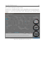
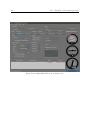
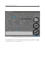
7.4 Graphical layout (GUI) - qml . . . . . . . . . . . .
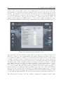
7.4.1 Home view . . . . . . . . . . . . . . . . . .
7.4.2 Parameters view . . . . . . . . . . . . . . .
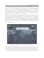
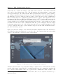
7.4.3 Still Camera view . . . . . . . . . . . . . .
7.4.4 Gimbal view . . . . . . . . . . . . . . . . .
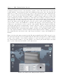
7.4.5 Objects view . . . . . . . . . . . . . . . . .
7.4.6 Exit view . . . . . . . . . . . . . . . . . . .
7.5 Safety during field operations . . . . . . . . . . . .
7.6 Requirements supported . . . . . . . . . . . . . . .
.
.
.
.
.
.
.
.
.
.
.
.
.
.
.
.
.
.
.
.
.
.
.
.
.
.
.
.
.
.
.
.
.
.
.
.
.
.
.
.
.
.
.
.
.
.
.
.
.
.
.
.
.
.
.
.
.
.
.
.
.
.
.
.
.
.
.
.
.
.
.
.
.
.
.
.
.
.
.
.
.
.
.
.
.
.
.
.
.
.
.
.
.
.
.
.
.
.
.
.
.
.
.
.
.
.
.
.
.
.
.
.
.
.
.
.
.
.
.
.
.
.
.
.
.
.
.
.
.
.
.
.
.
.
.
.
.
.
.
.
.
.
.
.
.
.
.
.
.
.
.
.
.
.
.
.
.
.
.
.
.
.
.
.
.
.
.
.
.
.
.
.
.
.
.
.
.
.
.
.
.
.
.
.
.
.
.
.
.
.
.
.
.
.
.
.
.
.
.
.
.
.
.
.
.
.
.
.
.
.
.
.
.
.
.
.
.
.
.
.
.
.
.
.
.
.
.
.
.
.
.
.
.
.
.
.
.
.
.
.
.
.
.
.
.
.
.
.
.
.
.
.
.
.
.
.
.
.
.
.
.
.
.
.
.
.
.
.
.
.
.
.
.
.
.
.
.
.
.
.
.
.
.
.
.
.
.
.
.
.
.
.
.
.
.
.
.
.
.
.
.
.
.
.
.
.
75
75
76
77
77
78
79
80
82
83
84
85
86
92
94
96
98
99
100
Contents
7.7
7.8
ix
Suggested improvements . . . . . . . . . . . . . . . . . . . . . . . . . . . . . . . . 100
Cross-compiling to Android . . . . . . . . . . . . . . . . . . . . . . . . . . . . . . 101
8 Simulation of the control system
8.1 Important results . . . . . . . . . . . . . . . . .
8.2 Number of iterations . . . . . . . . . . . . . . .
8.2.1 Maximum number of iterations set to 10
8.2.2 Maximum number of iterations set to 15
8.2.3 Maximum number of iterations set to 20
8.3 Long horizons . . . . . . . . . . . . . . . . . . .
8.3.1 Default values . . . . . . . . . . . . . . .
8.3.2 Horizon of 200 seconds . . . . . . . . . .
8.3.3 Horizon of 400 seconds . . . . . . . . . .
8.3.4 Horizon of 500 seconds . . . . . . . . . .
8.4 Short iteration steps . . . . . . . . . . . . . . .
8.5 Object selection . . . . . . . . . . . . . . . . . .
8.6 Dynamic clustering algorithm . . . . . . . . . .
8.6.1 Strict Distance Timer . . . . . . . . . .
8.7 Eight random objects . . . . . . . . . . . . . . .
8.7.1 GFV penalty . . . . . . . . . . . . . . .
8.7.2 Resources . . . . . . . . . . . . . . . . .
.
.
.
.
.
.
.
.
.
.
.
.
.
.
.
.
.
.
.
.
.
.
.
.
.
.
.
.
.
.
.
.
.
.
.
.
.
.
.
.
.
.
.
.
.
.
.
.
.
.
.
.
.
.
.
.
.
.
.
.
.
.
.
.
.
.
.
.
.
.
.
.
.
.
.
.
.
.
.
.
.
.
.
.
.
.
.
.
.
.
.
.
.
.
.
.
.
.
.
.
.
.
.
.
.
.
.
.
.
.
.
.
.
.
.
.
.
.
.
.
.
.
.
.
.
.
.
.
.
.
.
.
.
.
.
.
.
.
.
.
.
.
.
.
.
.
.
.
.
.
.
.
.
.
.
.
.
.
.
.
.
.
.
.
.
.
.
.
.
.
.
.
.
.
.
.
.
.
.
.
.
.
.
.
.
.
.
.
.
.
.
.
.
.
.
.
.
.
.
.
.
.
.
.
.
.
.
.
.
.
.
.
.
.
.
.
.
.
.
.
.
.
.
.
.
.
.
.
.
.
.
.
.
.
.
.
.
.
.
.
.
.
.
.
.
.
.
.
.
.
.
.
.
.
.
.
.
.
.
.
.
.
.
.
.
.
.
.
.
.
.
.
.
.
.
.
.
.
.
.
.
.
.
.
.
.
.
.
.
103
105
106
106
108
110
110
111
113
116
118
120
123
124
129
131
131
133
9 Hardware
9.1 Payload Overview . . . . . . . .
9.2 Payload Housing . . . . . . . . .
9.3 Power . . . . . . . . . . . . . . .
9.3.1 General overview . . . . .
9.3.2 Delay circuit . . . . . . .
9.3.3 Selectivity . . . . . . . . .
9.3.4 DC converters . . . . . . .
9.3.5 Piccolo interface . . . . .
9.3.6 Cut-off relay circuit . . .
9.4 On-board computation devices .
9.5 Still camera . . . . . . . . . . . .
9.5.1 Mounting the still camera
9.5.2 Designing wire damper for
9.5.3 First prototype . . . . . .
9.5.4 Second prototype . . . . .
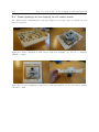
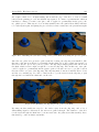
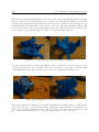
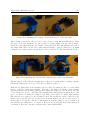
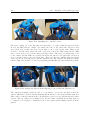
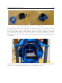
9.6 IR camera and gimbal . . . . . .
9.6.1 New gimbal design . . . .
9.7 Additional features . . . . . . . .
. . . . . . . . . . .
. . . . . . . . . . .
. . . . . . . . . . .
. . . . . . . . . . .
. . . . . . . . . . .
. . . . . . . . . . .
. . . . . . . . . . .
. . . . . . . . . . .
. . . . . . . . . . .
. . . . . . . . . . .
. . . . . . . . . . .
. . . . . . . . . . .
the camera mount
. . . . . . . . . . .
. . . . . . . . . . .
. . . . . . . . . . .
. . . . . . . . . . .
. . . . . . . . . . .
.
.
.
.
.
.
.
.
.
.
.
.
.
.
.
.
.
.
.
.
.
.
.
.
.
.
.
.
.
.
.
.
.
.
.
.
.
.
.
.
.
.
.
.
.
.
.
.
.
.
.
.
.
.
.
.
.
.
.
.
.
.
.
.
.
.
.
.
.
.
.
.
.
.
.
.
.
.
.
.
.
.
.
.
.
.
.
.
.
.
.
.
.
.
.
.
.
.
.
.
.
.
.
.
.
.
.
.
.
.
.
.
.
.
.
.
.
.
.
.
.
.
.
.
.
.
.
.
.
.
.
.
.
.
.
.
.
.
.
.
.
.
.
.
.
.
.
.
.
.
.
.
.
.
.
.
.
.
.
.
.
.
.
.
.
.
.
.
.
.
.
.
.
.
.
.
.
.
.
.
.
.
.
.
.
.
.
.
.
.
.
.
.
.
.
.
.
.
.
.
.
.
.
.
.
.
.
.
.
.
.
.
.
.
.
.
.
.
.
.
.
.
.
.
.
.
.
.
.
.
.
.
.
.
.
.
.
.
.
.
.
.
.
.
.
.
.
.
.
.
.
.
.
.
.
.
.
.
.
.
.
.
.
.
.
.
.
.
.
.
.
.
.
.
.
.
.
.
.
.
.
.
.
.
.
.
.
.
135
135
136
140
140
141
141
141
143
145
146
146
147
148
149
150
153
155
161
10 HIL Testing
10.1 HIL setup . . . . . . .
10.2 Power tests . . . . . .
10.2.1 Test procedure
10.2.2 Test results . .
.
.
.
.
.
.
.
.
.
.
.
.
.
.
.
.
.
.
.
.
.
.
.
.
.
.
.
.
.
.
.
.
.
.
.
.
.
.
.
.
.
.
.
.
.
.
.
.
.
.
.
.
.
.
.
.
.
.
.
.
.
.
.
.
.
.
.
.
163
163
165
166
166
.
.
.
.
.
.
.
.
.
.
.
.
.
.
.
.
.
.
.
.
.
.
.
.
.
.
.
.
.
.
.
.
.
.
.
.
.
.
.
.
.
.
.
.
.
.
.
.
.
.
.
.
.
.
.
.
.
.
.
.
.
.
.
.
.
.
.
.
.
.
.
.
.
.
.
.
.
.
.
.
.
.
.
.
.
.
.
.
.
.
.
.
.
.
.
.
.
.
x
Contents
10.3 Camera streams . . . . . .
10.3.1 Test procedure . .
10.3.2 Test results . . . .
10.4 Piccolo measurements and
10.4.1 Test procedure . .
10.4.2 Test results . . . .
10.5 Accuracy of the gimbal . .
10.5.1 Test procedure . .
10.5.2 Test results . . . .
10.6 External HMI . . . . . . .
10.6.1 Test procedure . .
10.6.2 Test results . . . .
10.7 Cut-off relay circuit . . . .
10.7.1 Test procedure . .
10.7.2 Test results . . . .
10.8 Simulations . . . . . . . .
10.8.1 Test procedure . .
10.8.2 Test results . . . .
. . . . . . . .
. . . . . . . .
. . . . . . . .
control action
. . . . . . . .
. . . . . . . .
. . . . . . . .
. . . . . . . .
. . . . . . . .
. . . . . . . .
. . . . . . . .
. . . . . . . .
. . . . . . . .
. . . . . . . .
. . . . . . . .
. . . . . . . .
. . . . . . . .
. . . . . . . .
11 Field Testing
11.1 Pre-flight check list . . . . . . . . . . .
11.2 The first day of field testing . . . . . .
11.2.1 Test procedure . . . . . . . . .
11.2.2 Test results . . . . . . . . . . .
11.3 The second day of field testing . . . .
11.3.1 Test procedure . . . . . . . . .
11.3.2 Test results . . . . . . . . . . .
11.4 The third day of field testing . . . . .
11.4.1 Test procedure . . . . . . . . .
11.4.2 Test results . . . . . . . . . . .
11.5 The forth day of field testing . . . . .
11.6 No flight tests with payload conducted
.
.
.
.
.
.
.
.
.
.
.
.
.
.
.
.
.
.
.
.
.
.
.
.
.
.
.
.
.
.
.
.
.
.
.
.
.
.
.
.
.
.
.
.
.
.
.
.
.
.
.
.
.
.
.
.
.
.
.
.
.
.
.
.
.
.
.
.
.
.
.
.
.
.
.
.
.
.
.
.
.
.
.
.
.
.
.
.
.
.
.
.
.
.
.
.
.
.
.
.
.
.
.
.
.
.
.
.
.
.
.
.
.
.
.
.
.
.
.
.
.
.
.
.
.
.
.
.
.
.
.
.
.
.
.
.
.
.
.
.
.
.
.
.
.
.
.
.
.
.
.
.
.
.
.
.
.
.
.
.
.
.
.
.
.
.
.
.
.
.
.
.
.
.
.
.
.
.
.
.
.
.
.
.
.
.
.
.
.
.
.
.
.
.
.
.
.
.
.
.
.
.
.
.
.
.
.
.
.
.
.
.
.
.
.
.
.
.
.
.
.
.
.
.
.
.
.
.
.
.
.
.
.
.
.
.
.
.
.
.
.
.
.
.
.
.
.
.
.
.
.
.
.
.
.
.
.
.
.
.
.
.
.
.
.
.
.
.
.
.
.
.
.
.
.
.
.
.
.
.
.
.
.
.
.
.
.
.
.
.
.
.
.
.
.
.
.
.
.
.
.
.
.
.
.
.
.
.
.
.
.
.
.
.
.
.
.
.
.
.
.
.
.
.
.
.
.
.
.
.
.
.
.
.
.
.
.
.
.
.
.
.
.
.
.
.
.
.
.
.
.
.
.
.
.
.
.
.
.
.
.
.
.
.
.
.
.
.
.
.
.
.
.
.
.
.
.
.
.
.
.
.
.
.
.
.
.
.
.
.
.
.
.
.
.
.
.
.
.
.
.
.
.
.
.
.
.
.
.
.
.
.
.
.
.
.
.
.
.
.
.
.
.
.
.
.
.
.
.
.
.
.
.
.
.
.
.
.
.
.
.
.
.
.
.
.
.
.
.
.
.
.
.
.
.
.
.
.
.
.
.
.
.
.
.
.
.
.
.
.
.
.
.
.
.
.
.
.
.
.
.
.
.
.
.
.
.
.
.
.
.
.
.
.
.
.
.
.
.
.
.
.
.
.
.
.
.
.
.
.
.
.
.
.
.
.
.
.
.
.
.
.
.
.
.
.
.
.
.
.
.
.
.
.
.
.
.
.
.
.
.
.
.
.
.
.
.
.
.
.
.
.
.
.
.
.
.
.
.
.
.
.
.
.
.
.
.
.
.
.
.
.
.
.
.
.
.
.
.
.
.
.
.
.
.
.
.
.
.
.
.
.
.
.
.
.
.
.
.
.
.
.
.
.
.
.
.
.
.
.
.
.
.
.
.
.
.
.
.
.
.
.
.
.
.
.
.
.
.
.
.
.
.
.
.
.
.
.
.
.
.
.
.
.
.
.
.
.
.
.
.
.
.
.
.
.
.
.
.
.
.
.
.
.
.
.
.
.
.
.
.
.
.
.
.
.
.
.
167
167
168
168
169
169
170
170
171
173
173
174
175
175
175
176
176
176
.
.
.
.
.
.
.
.
.
.
.
.
185
. 185
. 186
. 186
. 186
. 189
. 189
. 189
. 191
. 191
. 191
. 195
. 196
12 Conclusion
197
12.1 Review of system requirements . . . . . . . . . . . . . . . . . . . . . . . . . . . . 197
12.2 Findings . . . . . . . . . . . . . . . . . . . . . . . . . . . . . . . . . . . . . . . . . 200
13 Further work
Appendix A Implementation aspects
A.1 Estimated state IMC message . . . .
A.2 Json prepared object list message . .
A.3 Json prepared parameter information
A.4 Use of running engine in C++ . . .
A.5 Configuration file . . . . . . . . . . .
A.6 Simulation configuration file . . . . .
A.7 Monitoring system resources . . . . .
201
. . . . .
. . . . .
message
. . . . .
. . . . .
. . . . .
. . . . .
.
.
.
.
.
.
.
.
.
.
.
.
.
.
.
.
.
.
.
.
.
.
.
.
.
.
.
.
.
.
.
.
.
.
.
.
.
.
.
.
.
.
.
.
.
.
.
.
.
.
.
.
.
.
.
.
.
.
.
.
.
.
.
.
.
.
.
.
.
.
.
.
.
.
.
.
.
.
.
.
.
.
.
.
.
.
.
.
.
.
.
.
.
.
.
.
.
.
.
.
.
.
.
.
.
.
.
.
.
.
.
.
.
.
.
.
.
.
.
.
.
.
.
.
.
.
.
.
.
.
.
.
.
207
. 207
. 207
. 208
. 209
. 210
. 213
. 215
Contents
xi
Appendix B Hardware aspects
B.1 Payload housing . . . . . . . . . . . . . . . . . . . . . . .
B.2 Power . . . . . . . . . . . . . . . . . . . . . . . . . . . . .
B.3 First prototype of wire damping for still camera mount . .
B.4 Second prototype of wire damping for still camera mount
B.5 Gimbal calibration . . . . . . . . . . . . . . . . . . . . . .
B.6 Replacing the gimbal’s tilt servo . . . . . . . . . . . . . .
B.6.1 Manufacturers instructions . . . . . . . . . . . . .
B.6.2 Replacing the servo . . . . . . . . . . . . . . . . . .
B.7 Assembly of the gimbal prototype . . . . . . . . . . . . . .
B.7.1 Installing threaded inserts . . . . . . . . . . . . . .
B.7.2 Installing the new IMU . . . . . . . . . . . . . . .
B.7.3 Parts list for the gimbal . . . . . . . . . . . . . . .
B.7.4 GUI for calibrating the gimbal controller . . . . . .
B.7.5 Wiring diagram . . . . . . . . . . . . . . . . . . . .
B.8 MPU6050 IMU tester . . . . . . . . . . . . . . . . . . . .
Appendix C Specifications of components and devices
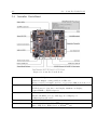
C.1 UAV: Penguin B . . . . . . . . . . . . . . . . . . . . .
C.1.1 Product Specification . . . . . . . . . . . . . .
C.1.2 Performance . . . . . . . . . . . . . . . . . . . .
C.2 Piccolo SL autopilot . . . . . . . . . . . . . . . . . . .
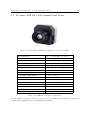
C.3 IR Camera: FLIR Tau 2 (640) Uncooled Cores 19 mm
C.4 Tau PCB Wearsaver . . . . . . . . . . . . . . . . . . .
C.5 Gimbal: BTC-88 . . . . . . . . . . . . . . . . . . . . .
C.6 Controller: Panda Board . . . . . . . . . . . . . . . . .
C.7 DFRobot Relay Module V2 . . . . . . . . . . . . . . .
C.8 AXIS M7001 Video Encoder . . . . . . . . . . . . . . .
C.9 DSP TMDSEVM6678L . . . . . . . . . . . . . . . . .
C.10 Arecont AV10115v1 . . . . . . . . . . . . . . . . . . .
C.11 Tamron lens M118FM08 . . . . . . . . . . . . . . . . .
C.12 Trendnet TE100-S5 Fast Ethernet Switch . . . . . . .
C.13 Rocket M5 . . . . . . . . . . . . . . . . . . . . . . . . .
Bibliography
.
.
.
.
.
.
.
.
.
.
.
.
.
.
.
.
.
.
.
.
.
.
.
.
.
.
.
.
.
.
.
.
.
.
.
.
.
.
.
.
.
.
.
.
.
.
.
.
.
.
.
.
.
.
.
.
.
.
.
.
.
.
.
.
.
.
.
.
.
.
.
.
.
.
.
.
.
.
.
.
.
.
.
.
.
.
.
.
.
.
.
.
.
.
.
.
.
.
.
.
.
.
.
.
.
.
.
.
.
.
.
.
.
.
.
.
.
.
.
.
.
.
.
.
.
.
.
.
.
.
.
.
.
.
.
.
.
.
.
.
.
.
.
.
.
.
.
.
.
.
.
.
.
.
.
.
.
.
.
.
.
.
.
.
.
.
.
.
.
.
.
.
.
.
.
.
.
.
.
.
.
.
.
.
.
.
.
.
.
.
.
.
.
.
.
.
.
.
.
.
.
.
.
.
.
.
.
.
.
.
.
.
.
.
.
.
.
.
.
.
.
.
.
.
.
.
.
.
.
.
.
.
.
.
.
.
.
.
.
.
.
.
.
.
.
.
.
.
.
.
.
.
.
.
.
.
.
.
.
.
.
.
.
.
.
.
.
.
.
.
.
.
.
.
.
.
.
.
.
.
.
.
.
.
.
.
.
.
.
.
.
.
.
.
.
.
.
.
.
.
.
.
.
.
.
.
.
.
.
.
.
.
.
.
.
.
.
.
.
.
.
.
.
.
.
.
.
.
.
.
.
.
.
.
.
.
.
.
.
.
.
.
.
.
.
.
.
.
.
.
.
.
.
.
.
.
.
.
.
.
.
.
.
.
.
.
.
.
.
.
.
.
.
.
.
219
. 219
. 221
. 223
. 224
. 225
. 227
. 227
. 227
. 232
. 238
. 239
. 240
. 241
. 244
. 245
.
.
.
.
.
.
.
.
.
.
.
.
.
.
.
249
. 249
. 250
. 250
. 251
. 253
. 254
. 255
. 256
. 258
. 259
. 261
. 262
. 263
. 264
. 265
267
xii
Contents
List of Figures
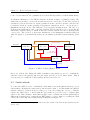
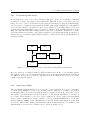
1.1
System topology. . . . . . . . . . . . . . . . . . . . . . . . . . . . . . . . . . . . .
5
2.1
2.2
Example of aerial object detection. . . . . . . . . . . . . . . . . . . . . . . . . . .
Example of grassroots mapping. . . . . . . . . . . . . . . . . . . . . . . . . . . . .
8
8
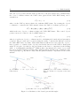
3.1
3.2
3.3
3.4
3.5
3.6
Illustration of some of the coordinate frames used in the object tracking system.
Calculation of CO’s and gimbal’s positions relative earth. . . . . . . . . . . . . .
The gimbal’s body frame {g}. . . . . . . . . . . . . . . . . . . . . . . . . . . . . .
Coordinate systems and geoid representation. . . . . . . . . . . . . . . . . . . . .
From a local ENU frame to geographical coordinates (google maps). . . . . . . .
An aircraft executing a coordinated, level turn (Leven et al., 2009). . . . . . . . .
12
14
15
17
20
22
4.1
4.2
4.3
4.4
4.5
4.6
The camera frame {c,b} in zero position, i.e. {c,b} equals {c,e}. . . . .
Rotation of the camera image’s projected pyramid. . . . . . . . . . . .
Projection of the camera image with a pitch angle of 30◦ . . . . . . . .
Projection of the camera image with a roll angle of 30◦ . . . . . . . . .
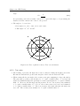
Illustration of the same side test. . . . . . . . . . . . . . . . . . . . . .
The same side test used in a ground field of view (GFV) with multiple
. . . . .
. . . . .
. . . . .
. . . . .
. . . . .
objects.
.
.
.
.
.
.
25
26
28
29
29
31
5.1
5.2
5.3
5.4
5.5
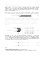
MPC - Scheme (Hauger, 2013). . . . . . . . . . . . . . . . . . .
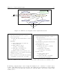
Calculation of the desired pan and tilt angles. . . . . . . . . . .
UML state diagram: Object planning. . . . . . . . . . . . . . .
Simplified representation of αd . . . . . . . . . . . . . . . . . . .
Proposed feed forward compensation using IMU measurements.
.
.
.
.
.
.
.
.
.
.
35
36
41
42
46
6.1
6.2
6.3
6.4
6.5
6.6
6.7
6.8
6.9
6.10
Object tracking system. . . . . . . . . . . . . . . . . . . . . . . . . . . . . . . . .
UML Use-case diagram: Control system interactions. . . . . . . . . . . . . . . . .
UML Use-case textual scenarios: Main scenario with extension for manual control.
UML Use-case textual scenario: Extension for semi-automatic control. . . . . . .
UML state diagram: Multi-threaded system architecture. . . . . . . . . . . . . .
UML sequence diagram: Asynchronous system architecture. . . . . . . . . . . . .
Threaded communication structure. . . . . . . . . . . . . . . . . . . . . . . . . .
UML state machine: The engine’s system architecture. . . . . . . . . . . . . . . .
Threaded communication structure with a Kalman filter module. . . . . . . . . .
UML component diagram: .hpp/.h file dependencies. . . . . . . . . . . . . . . .
50
53
53
54
55
57
58
60
69
73
7.1
7.2
7.3
7.4
Simplified HMI architecture. . .
Listener: Input message flow. .
Worker: Ouptut message flow. .
HMI architecture: Sub-classing.
78
79
80
81
.
.
.
.
.
.
.
.
.
.
.
.
.
.
.
.
.
.
.
.
xiii
.
.
.
.
.
.
.
.
.
.
.
.
.
.
.
.
.
.
.
.
.
.
.
.
.
.
.
.
.
.
.
.
.
.
.
.
.
.
.
.
.
.
.
.
.
.
.
.
.
.
.
.
.
.
.
.
.
.
.
.
.
.
.
.
.
.
.
.
.
.
.
.
.
.
.
.
.
.
.
.
.
.
.
.
.
.
.
.
.
.
.
.
.
.
.
.
.
.
.
.
.
.
.
.
.
.
.
.
.
.
.
.
.
.
.
.
.
.
.
.
.
.
.
.
.
.
.
.
.
.
.
.
xiv
List of Figures
7.5
7.6
7.7
7.8
7.9
7.10
7.11
7.12
7.13
7.14
7.15
7.16
7.17
7.18
7.19
7.20
7.21
7.22
8.1
8.2
8.3
8.4
8.5
8.6
8.7
8.8
8.9
8.10
8.11
8.12
8.13
8.14
8.15
8.16
8.17
8.18
8.19
8.20
8.21
Message flow when removing an object from the object list. . . . . . . . . . . .
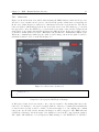
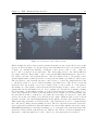
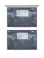
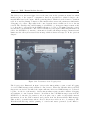
Home view: No connection. . . . . . . . . . . . . . . . . . . . . . . . . . . . . .
Home view: Connected. . . . . . . . . . . . . . . . . . . . . . . . . . . . . . . .
Parameters view: Network view. . . . . . . . . . . . . . . . . . . . . . . . . . .
Parameters view: System Modes view. . . . . . . . . . . . . . . . . . . . . . . .
Parameters view: Debug view. . . . . . . . . . . . . . . . . . . . . . . . . . . .
Parameters view: Logging view. . . . . . . . . . . . . . . . . . . . . . . . . . . .
Parameters view: Parameters view. . . . . . . . . . . . . . . . . . . . . . . . . .
Parameters view: Limits view. . . . . . . . . . . . . . . . . . . . . . . . . . . .
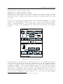
Still Camera view: No image stream connected. . . . . . . . . . . . . . . . . . .
Still Camera view: Image stream connected. . . . . . . . . . . . . . . . . . . . .
Gimbal view: No image stream connected. . . . . . . . . . . . . . . . . . . . . .
Gimbal view: Image stream connected. . . . . . . . . . . . . . . . . . . . . . . .
Objects view: No image stream connected and no connection to the control system
(engine). . . . . . . . . . . . . . . . . . . . . . . . . . . . . . . . . . . . . . . . .
Objects view: No image stream connected. . . . . . . . . . . . . . . . . . . . . .
Objects view: Image stream connected. . . . . . . . . . . . . . . . . . . . . . . .
Exit view. . . . . . . . . . . . . . . . . . . . . . . . . . . . . . . . . . . . . . . .
HMI deployed to an Asus Transformer tablet. . . . . . . . . . . . . . . . . . . .
.
.
.
.
.
.
.
.
.
.
.
.
.
83
84
85
87
88
88
89
90
91
92
93
94
95
.
.
.
.
.
96
97
98
99
101
Example of a North-East plot with attitude plots. . . . . . . . . . . . . . . . . .
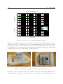
Iteration test. Max number of iterations = 10. Step = 158. . . . . . . . . . . . .
Iteration test. Max number of iterations = 10. Step = 257. . . . . . . . . . . . .
Iteration test. Max number of iterations = 15. Step = 58. . . . . . . . . . . . . .
Iteration test. Max number of iterations = 15. Step = 59. . . . . . . . . . . . . .
Iteration test. Max number of iterations = 15. Step = 60. . . . . . . . . . . . . .
Long Horizon test. Default ACADO parameters. Step = 389. . . . . . . . . . . .
Long Horizon test. Default ACADO parameters. Step = 419. . . . . . . . . . . .
Long Horizon test. Default ACADO parameters. Step = 495. . . . . . . . . . . .
Long Horizon test. Time horizon = 200 sec. Max iteration length = 10 sec. Step
= 34. . . . . . . . . . . . . . . . . . . . . . . . . . . . . . . . . . . . . . . . . . . .
Long Horizon test. Time horizon = 200 sec. Max iteration length = 10 sec. Step
= 41. . . . . . . . . . . . . . . . . . . . . . . . . . . . . . . . . . . . . . . . . . . .
Long Horizon test. Time horizon = 200 sec. Max iteration length = 10 sec. Step
= 57. . . . . . . . . . . . . . . . . . . . . . . . . . . . . . . . . . . . . . . . . . . .
Long Horizon test. Time horizon = 200 sec. Max number of iterations = 1. Step
= 30. . . . . . . . . . . . . . . . . . . . . . . . . . . . . . . . . . . . . . . . . . . .
Horizon test. Time horizon = 400 sec. Max iteration length = 10 sec. Step = 38.
Horizon test. Time horizon = 400 sec. Max iteration length = 10 sec. Step = 43.
Horizon test. Time horizon = 400 sec. Max iteration length = 10 sec. Step = 77.
Long Horizon test. Time horizon = 500 sec. Max iteration length = 5 sec. Step
= 83. . . . . . . . . . . . . . . . . . . . . . . . . . . . . . . . . . . . . . . . . . . .
Long Horizon test. Time horizon = 500 sec. Max iteration length = 5 sec. Step
= 131. . . . . . . . . . . . . . . . . . . . . . . . . . . . . . . . . . . . . . . . . . .
Comparison in paths. . . . . . . . . . . . . . . . . . . . . . . . . . . . . . . . . . .
Short step length. Step = 3629. . . . . . . . . . . . . . . . . . . . . . . . . . . . .
Short step length. Step = 3693. . . . . . . . . . . . . . . . . . . . . . . . . . . . .
104
107
108
109
109
109
111
112
112
113
114
114
116
117
117
117
119
119
120
122
122
List of Figures
8.22
8.23
8.24
8.25
8.26
8.27
8.28
8.29
8.30
8.31
8.32
8.33
8.34
8.35
8.36
8.37
8.38
8.39
9.1
9.2
9.3
9.4
9.5
9.6
9.7
9.8
9.9
9.10
9.11
9.12
9.13
9.14
9.15
9.16
9.17
9.18
9.19
9.20
xv
Reference plot with the default ACADO parameters. Step = 331. . . . . . . . .
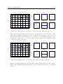
Object selection with our defult ACADO parameters. Step = 2. . . . . . . . . .
Grouping. Step = 360. . . . . . . . . . . . . . . . . . . . . . . . . . . . . . . . .
Grouping. Step = 850. . . . . . . . . . . . . . . . . . . . . . . . . . . . . . . . .
Grouping. Step = 851. . . . . . . . . . . . . . . . . . . . . . . . . . . . . . . . .
Grouping. Step = 852. . . . . . . . . . . . . . . . . . . . . . . . . . . . . . . . .
Grouping. Step = 1056. . . . . . . . . . . . . . . . . . . . . . . . . . . . . . . .
Grouping. Step = 1057. . . . . . . . . . . . . . . . . . . . . . . . . . . . . . . .
Grouping. Step = 1058. . . . . . . . . . . . . . . . . . . . . . . . . . . . . . . .
Grouping. Step = 1252. . . . . . . . . . . . . . . . . . . . . . . . . . . . . . . .
Grouping, strict timer. Step = 123 . . . . . . . . . . . . . . . . . . . . . . . . .
Grouping, strict timer. Step = 139. . . . . . . . . . . . . . . . . . . . . . . . . .
Grouping, strict timer. Step = 159. . . . . . . . . . . . . . . . . . . . . . . . . .
Eight random objects with the GFV penalty disabled. Step = 1300. . . . . . .
Eight random objects with the GFV penalty disabled. Step = 1398. . . . . . .
Eight random objects with the GFV penalty enabled. Step = 1300. . . . . . . .
Eight random objects with the GFV penalty enabled. Step = 1398. . . . . . . .
CPU and memory usage plots of the control system with and without the MPC
running. . . . . . . . . . . . . . . . . . . . . . . . . . . . . . . . . . . . . . . . .
.
.
.
.
.
.
.
.
.
.
.
.
.
.
.
.
.
122
123
125
126
126
127
127
127
128
128
129
130
130
131
132
132
133
The payload’s signal flow. . . . . . . . . . . . . . . . . . . . . . . . . . . . . . .
Sketch of the payload housing. . . . . . . . . . . . . . . . . . . . . . . . . . . .
The power distribution as it appeared prior to second field test, after the
converters and terminal blocks were replaced. . . . . . . . . . . . . . . . . . . .
Components assembled in the payload housing. . . . . . . . . . . . . . . . . . .
Components mounted on the payload housing’s lid. . . . . . . . . . . . . . . . .
The payload’s power distribution, second version. The DFRobot Relay Module
V2 is highly simplified in this figure. This is more of a principle sketch of the
relay module’s functionality. See appendix C.7 for more information regarding
the relay circuit from DFRobot. . . . . . . . . . . . . . . . . . . . . . . . . . . .
The new overpowered step-up converter with large heat sink. . . . . . . . . . .
Low voltage tests. . . . . . . . . . . . . . . . . . . . . . . . . . . . . . . . . . . .
UAV-Piccolo infrastructure. . . . . . . . . . . . . . . . . . . . . . . . . . . . . .
Rendering of the camera mount version 1. Designed and rendered in Rhino 3D.
The camera mount installed in the fuselage. . . . . . . . . . . . . . . . . . . . .
Commercial wire vibration isolators. . . . . . . . . . . . . . . . . . . . . . . . .
Rendering of wire vibration isolating camera mount. Designed and rendered in
Rhino 3D. . . . . . . . . . . . . . . . . . . . . . . . . . . . . . . . . . . . . . . .
Designing and printing a new camera mount, second prototype. . . . . . . . . .
Bode plots of a mass-spring-damper system. . . . . . . . . . . . . . . . . . . . .
Final wire configuration with 1.5mm electrical wire. . . . . . . . . . . . . . . .
Gimbal mounted in UAV. . . . . . . . . . . . . . . . . . . . . . . . . . . . . . .
Wire problems in gimbal. . . . . . . . . . . . . . . . . . . . . . . . . . . . . . .
Rendering of the first prototype: 3-axis 3D printable gimbal. . . . . . . . . . .
The gimbal prototype fully assembled with camera installed. . . . . . . . . . . .
. 135
. 136
. 134
. 137
. 138
. 139
.
.
.
.
.
.
.
140
142
143
144
147
148
148
.
.
.
.
.
.
.
.
149
150
152
152
153
154
158
160
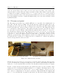
10.1 HIL hardware setup. . . . . . . . . . . . . . . . . . . . . . . . . . . . . . . . . . . 163
xvi
List of Figures
10.2 HIL software setup. . . . . . . . . . . . . . . . . . . . . . . . . . . . . . . . . . .
10.3 Payload installed in the UAV. . . . . . . . . . . . . . . . . . . . . . . . . . . . .
10.4 Test of gimbal accuracy: Test case schematics. . . . . . . . . . . . . . . . . . .
10.5 PandaBoard’s GPIO (PandaBoard.org, 2010). . . . . . . . . . . . . . . . . . . .
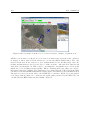
10.6 Four stationary objects. 35 control steps were sent to the Piccolo. . . . . . . . .
10.7 Four stationary objects. 115 control steps were sent to the Piccolo. . . . . . . .
10.8 Four stationary objects. 317 control steps were sent to the Piccolo. . . . . . . .
10.9 Four stationary objects. 846 control steps were sent to the Piccolo. . . . . . . .
10.10Screenshot of the Piccolo Command Center, entering circular motion for the third
tracked object. . . . . . . . . . . . . . . . . . . . . . . . . . . . . . . . . . . . .
10.11Four moving objects. 220 control steps were sent to the Piccolo. . . . . . . . . .
10.12Four moving objects. 342 control steps were sent to the Piccolo. . . . . . . . . .
10.13Four moving objects. 753 control steps were sent to the Piccolo. . . . . . . . . .
10.14Four moving objects. 1273 control steps were sent to the Piccolo. . . . . . . . .
10.15Screenshot of the Piccolo Command Center, example of spiral motion. . . . . .
10.16Eight moving objects. 125 control steps were sent to the Piccolo. . . . . . . . .
10.17Eight moving objects. 290 control steps were sent to the Piccolo. . . . . . . . .
10.18Eight moving objects. 1165 control steps were sent to the Piccolo. . . . . . . .
10.19Eight moving objects. 1533 control steps were sent to the Piccolo. . . . . . . .
10.20Screenshot from the Piccolo Command Center, example of spiral motion. . . .
.
.
.
.
.
.
.
.
164
165
171
175
176
177
177
178
.
.
.
.
.
.
.
.
.
.
.
178
179
179
180
180
181
182
182
183
183
184
11.1
11.2
11.3
11.4
11.5
11.6
11.7
11.8
11.9
Installation of the payload in the UAV before the taxing tests. . . .
Preparation of Penguin B. . . . . . . . . . . . . . . . . . . . . . . . .
Piccolo mounted in two different directions in the UAV. . . . . . . .
Three stationary objects. 59 control steps were sent to the Piccolo. .
Three stationary objects. 206 control steps were sent to the Piccolo.
Three stationary objects. 298 control steps were sent to the Piccolo.
Three stationary objects. 375 control steps were sent to the Piccolo.
Three stationary objects. 451 control steps were sent to the Piccolo.
First flight test without the object tracking system’s payload. . . . .
.
.
.
.
.
.
.
.
.
187
190
192
193
193
194
194
195
196
B.1
B.2
B.3
B.4
The payload housing’s lid. . . . . . . . . . . . . . . . . . . . . . . . . . . . . . .
The unfolded payload housing base. . . . . . . . . . . . . . . . . . . . . . . . .
The payload’s power distribution. Early layout. . . . . . . . . . . . . . . . . . .
The payload’s power distribution. Early layout as it appeared installed in the
payload housing. . . . . . . . . . . . . . . . . . . . . . . . . . . . . . . . . . . .
Proposed improvements to the payload’s power distribution with fuses and
improved Piccolo/payload interface. . . . . . . . . . . . . . . . . . . . . . . . .
First prototype of the wire dampened camera mount. Unsuitable for further
testing. . . . . . . . . . . . . . . . . . . . . . . . . . . . . . . . . . . . . . . . .
First configuration, with bicycle brake wire in half loops. Proved too stiff and
difficult to adjust. . . . . . . . . . . . . . . . . . . . . . . . . . . . . . . . . . . .
Second configuration, with bicycle brake wire in full loops. Proved easier to
adjust, but still too stiff. . . . . . . . . . . . . . . . . . . . . . . . . . . . . . . .
Laser mount for calibration of gimbal angles. . . . . . . . . . . . . . . . . . . .
Camera with sturdier mounting screws, USB and coax connectors. . . . . . . .
B.5
B.6
B.7
B.8
B.9
B.10
.
.
.
.
.
.
.
.
.
.
.
.
.
.
.
.
.
.
.
.
.
.
.
.
.
.
.
.
.
.
.
.
.
.
.
.
.
.
.
.
.
.
.
.
.
.
.
.
.
.
.
.
.
.
. 219
. 220
. 221
. 221
. 222
. 223
. 224
. 224
. 225
. 228
List of Figures
xvii
B.11 Gimbal without camera. Notice the two hex bolts holding the gear and yoke
inside, as well as the white mark indicating the alignment of the gears. . . . . . . 228
B.12 Removing the large gear and separating the ball from the rest of the gimbal. . . 229
B.13 Removing the servo from the ball. . . . . . . . . . . . . . . . . . . . . . . . . . . 229
B.14 Removing the gear from the servo. . . . . . . . . . . . . . . . . . . . . . . . . . . 230
B.15 Replacing tilt servo in the gimbal. . . . . . . . . . . . . . . . . . . . . . . . . . . 231
B.16 Most of the gimbal’s parts laid out, including slip ring, motors and controller.
The camera mounting bracket and the threaded brass inserts are missing. . . . . 232
B.17 Installing the yaw axis bearing on the geared shaft and joining the pieces together.233
B.18 Installing the slip ring in the geared yaw shaft. . . . . . . . . . . . . . . . . . . . 233
B.19 Joining the fork to the upper support assembly. . . . . . . . . . . . . . . . . . . . 234
B.20 Installing the yaw motor and the motor gear. . . . . . . . . . . . . . . . . . . . . 234
B.21 Installing the bearing, roll and pitch motors on the pitch arm. . . . . . . . . . . . 235
B.22 Installing the roll arm and joining the upper and lower assemblies. . . . . . . . . 235
B.23 Installing the controller boards. . . . . . . . . . . . . . . . . . . . . . . . . . . . . 236
B.24 Splicing the wires from the slip ring to the roll and the pitch motors. . . . . . . . 236
B.25 Installing the bracket on the IR camera. . . . . . . . . . . . . . . . . . . . . . . . 237
B.26 Test fit with the camera. The camera is not connected and the IMU is not
installed yet. One of the ball halves is resting in its place for illustrative purposes.237
B.27 insert being installed in upper support structure. . . . . . . . . . . . . . . . . . . 238
B.28 The new IMU installed on the newly printed roll arm. . . . . . . . . . . . . . . . 239
B.29 SimpleBGS GUI v2.30: Basic tab. . . . . . . . . . . . . . . . . . . . . . . . . . . 241
B.30 SimpleBGS GUI v2.30: Advanced tab. . . . . . . . . . . . . . . . . . . . . . . . . 242
B.31 SimpleBGS GUI v2.30: RC settings tab. . . . . . . . . . . . . . . . . . . . . . . . 243
B.32 Wiring diagram for the gimbal prototype. . . . . . . . . . . . . . . . . . . . . . . 244
B.33 MPU6050 IMU tester. . . . . . . . . . . . . . . . . . . . . . . . . . . . . . . . . . 245
C.1 UAV Penguin B. . . . . . . . . . . . . . . . . . . . . . . . .
C.2 Piccolo SL autopilot, provided by Cloud Cap Technology. .
C.3 IR Camera: FLIR Tau 2 (640) Uncooled Cores 19mm. . . .
C.4 Wearsaver PCB for FLIR Tau IR camera. . . . . . . . . . .
C.5 Wearsaver PCB for FLIR Tau IR camera. . . . . . . . . . .
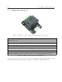
C.6 Gimbal: BTC-88. . . . . . . . . . . . . . . . . . . . . . . . .
C.7 Gimbal BTC-88: Dimensions. . . . . . . . . . . . . . . . . .
C.8 Controller: Panda Board. . . . . . . . . . . . . . . . . . . .
C.9 DFRobot relay circuit used in the payload’s cut-off circuit.
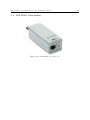
C.10 Axis M7001 Video Encoder. . . . . . . . . . . . . . . . . . .
C.11 DSP TMDSEVM6678L. . . . . . . . . . . . . . . . . . . . .
C.12 Arecont AV10115v1. . . . . . . . . . . . . . . . . . . . . . .
C.13 Tamron M118FM08. . . . . . . . . . . . . . . . . . . . . . .
C.14 Trendnet TE100-S5. . . . . . . . . . . . . . . . . . . . . . .
C.15 Ubiquiti Networks: Rocket M5 . . . . . . . . . . . . . . .
.
.
.
.
.
.
.
.
.
.
.
.
.
.
.
.
.
.
.
.
.
.
.
.
.
.
.
.
.
.
.
.
.
.
.
.
.
.
.
.
.
.
.
.
.
.
.
.
.
.
.
.
.
.
.
.
.
.
.
.
.
.
.
.
.
.
.
.
.
.
.
.
.
.
.
.
.
.
.
.
.
.
.
.
.
.
.
.
.
.
.
.
.
.
.
.
.
.
.
.
.
.
.
.
.
.
.
.
.
.
.
.
.
.
.
.
.
.
.
.
.
.
.
.
.
.
.
.
.
.
.
.
.
.
.
.
.
.
.
.
.
.
.
.
.
.
.
.
.
.
.
.
.
.
.
.
.
.
.
.
.
.
.
.
.
.
.
.
.
.
.
.
.
.
.
.
.
.
.
.
249
251
253
254
254
255
255
256
258
259
261
262
263
264
265
xviii
List of Figures
List of Tables
3.1
WGS-84 parameters (Fossen, 2011a). . . . . . . . . . . . . . . . . . . . . . . . . . 18
6.1
6.2
6.3
Servo addresses related to the gimbal. . . . . . . . . . . . . . . . . . . . . . . . . 61
IMC ControlLoops message. . . . . . . . . . . . . . . . . . . . . . . . . . . . . . . 61
IMC DesiredPath message. . . . . . . . . . . . . . . . . . . . . . . . . . . . . . . . 62
8.1
8.2
8.3
8.4
8.5
8.6
8.7
8.8
8.9
8.10
8.11
Default ACADO OCP parameters. . . . . . . . . . . . . . . . . . . . . . . . . . . 105
The UAV’s and the objects’ initial values. . . . . . . . . . . . . . . . . . . . . . . 106
ACADO OCP parameters: Max iterations is set to 10. . . . . . . . . . . . . . . . 106
Time consumption: Max iterations is set to 10. . . . . . . . . . . . . . . . . . . . 107
ACADO OCP parameters: Max iterations is set to 15. . . . . . . . . . . . . . . . 108
Time consumption: Max iterations is set to 15. . . . . . . . . . . . . . . . . . . . 108
Time consumption: Default ACADO parameters. . . . . . . . . . . . . . . . . . . 110
Long horizon: Initial values for the UAV and the object. . . . . . . . . . . . . . . 111
ACADO OCP parameters: Default ACADO parameters. . . . . . . . . . . . . . . 111
Time consumption: Default ACADO parameters. . . . . . . . . . . . . . . . . . . 111
ACADO OCP parameters: 200 seconds time horizon. Max iteration length of 10
seconds. . . . . . . . . . . . . . . . . . . . . . . . . . . . . . . . . . . . . . . . . . 113
Time consumption: 200 seconds time horizon. Max iteration length of 10 seconds.113
ACADO OCP parameters: Time horizon is set to 200. . . . . . . . . . . . . . . . 114
Time consumption: 200 seconds time horizon. . . . . . . . . . . . . . . . . . . . . 115
ACADO OCP parameters: 200 seconds time horizon. Max number of iterations
is set to 1. . . . . . . . . . . . . . . . . . . . . . . . . . . . . . . . . . . . . . . . . 115
Time consumption: 200 seconds time horizon. Max number of iterations is set
to 1. . . . . . . . . . . . . . . . . . . . . . . . . . . . . . . . . . . . . . . . . . . . 115
ACADO OCP parameters: 400 seconds time horizon. Max iteration length of 10
sec. . . . . . . . . . . . . . . . . . . . . . . . . . . . . . . . . . . . . . . . . . . . . 116
Time consumption: 400 seconds time horizon. Max iteration length of 10 sec. . . 116
ACADO OCP parameters: Time horizon of 500 sec. Max iteration length of 5 sec.118
Time consumption: Time horizon of 500 sec. Max iteration length of 5 sec. . . . 118
Short step: The UAV’s and the objects’ initial values. . . . . . . . . . . . . . . . 121
ACADO OCP parameters: Max iteration length of 0.1 sec. . . . . . . . . . . . . 121
ACADO OCP parameters: Max iteration length of 0.1 sec. Time horizon of 5 sec.121
Time consumption: Three objects moving. . . . . . . . . . . . . . . . . . . . . . . 121
Short step: Initial values for UAV and object. . . . . . . . . . . . . . . . . . . . . 123
Grouping: The UAV’s and objects’ initial values. . . . . . . . . . . . . . . . . . . 124
ACADO OCP parameters: Default ACADO parameters. . . . . . . . . . . . . . . 124
Time consumption: Three objects moving. . . . . . . . . . . . . . . . . . . . . . . 125
ACADO OCP parameters: Default ACADO parameters. . . . . . . . . . . . . . . 131
8.12
8.13
8.14
8.15
8.16
8.17
8.18
8.19
8.20
8.21
8.22
8.23
8.24
8.25
8.26
8.27
8.28
8.29
xix
xx
List of Tables
8.30 Time consumption: Eight random objects moving with the GFV penalty disabled.131
8.31 Time consumption: Eight random objects moving with the GFV penalty enabled. 132
10.1 Gimbal’s pan and tilt accuracy. . . . . . . . . . . . . . . . . . . . . . . . . . . . . 172
A.1
A.2
A.3
A.4
System configuration file details. . . . . . .
System configuration file details. . . . . . .
Simulation configuration file details. . . . .
Description of ps-flags used in script A.20. .
.
.
.
.
.
.
.
.
.
.
.
.
.
.
.
.
.
.
.
.
.
.
.
.
.
.
.
.
.
.
.
.
.
.
.
.
.
.
.
.
.
.
.
.
.
.
.
.
.
.
.
.
.
.
.
.
.
.
.
.
.
.
.
.
.
.
.
.
.
.
.
.
.
.
.
.
.
.
.
.
.
.
.
.
212
213
215
216
B.1 Parts list for the gimbal. . . . . . . . . . . . . . . . . . . . . . . . . . . . . . . . . 240
B.2 MPU6050 IMU tester components. . . . . . . . . . . . . . . . . . . . . . . . . . . 245
C.1 UAV Penguin B: Product specifications. .
C.2 UAV Penguin B: Performance. . . . . . .
C.3 Piccolo SL autopilot. . . . . . . . . . . . .
C.4 FLIR Tau 2 (640): Specifications. . . . . .
C.5 Gimbal BTC-88: Specifications. . . . . . .
C.6 Panda Board: Specifications. . . . . . . .
C.7 DFRobot relay module V2 specifications.
C.8 AXIS M7001: Specifications. . . . . . . .
C.9 DSP TMDSEVM6678L: Features. . . . . .
C.10 Arecont AV10115v1: Features. . . . . . .
C.11 Tamron M118FM08: Specifications. . . . .
C.12 Trendnet TE100-S5: Specifications. . . . .
C.13 Rocket M5: Specifications. . . . . . . . . .
.
.
.
.
.
.
.
.
.
.
.
.
.
.
.
.
.
.
.
.
.
.
.
.
.
.
.
.
.
.
.
.
.
.
.
.
.
.
.
.
.
.
.
.
.
.
.
.
.
.
.
.
.
.
.
.
.
.
.
.
.
.
.
.
.
.
.
.
.
.
.
.
.
.
.
.
.
.
.
.
.
.
.
.
.
.
.
.
.
.
.
.
.
.
.
.
.
.
.
.
.
.
.
.
.
.
.
.
.
.
.
.
.
.
.
.
.
.
.
.
.
.
.
.
.
.
.
.
.
.
.
.
.
.
.
.
.
.
.
.
.
.
.
.
.
.
.
.
.
.
.
.
.
.
.
.
.
.
.
.
.
.
.
.
.
.
.
.
.
.
.
.
.
.
.
.
.
.
.
.
.
.
.
.
.
.
.
.
.
.
.
.
.
.
.
.
.
.
.
.
.
.
.
.
.
.
.
.
.
.
.
.
.
.
.
.
.
.
.
.
.
.
.
.
.
.
.
.
.
.
.
.
.
.
.
.
.
.
.
.
.
.
.
.
.
.
.
.
.
.
.
.
.
.
.
.
.
.
.
.
.
.
.
.
.
.
.
.
.
.
.
.
.
.
.
.
.
.
.
.
.
.
.
.
.
.
250
250
252
253
255
257
258
260
261
262
263
264
265
Nomenclature
Abbreviations
CAN Controller Area Network
IMU Inertial Measurement Unit
CG
Center of Gravity
INS
Inertial Navigation System
CL
Coefficient of Lift
IP
Internet Protocol
CO
Center of Origin
IR
InfraRed
LQR Linear Quadratic Regulator
CPU Central Processing Unit
CV
LSQ Least Squares Quadratic
Computer Vision
MHE Moving Horizon Estimator
DOF Degrees of freedom
DP
MILP Mixed-Integer Linear Programming
Dynamic Positioning
MPC Model Predictive Controller
ECEF Earth Center Earth Fixed
MPF Marginalized Particle Filter
EMC ElectroMagnetic Compability
MTOW Maximum TakeOff Weight
ENU East North Up
MV
EO
NED North East Down
Electro-Optic
Machine Vision
NMPC Nonlinear Model Predictive
Control
FAT Factory Acceptance Test
GFV Ground Field of View
OMG Object Management Group
GPIO General-Purpose Input/Output
OO
GPS Global Positioning System
PCB Printable Circuit Board
GUI Graphical User Interface
PDF Probability Density Function
HIL
PMS Power Management System
Hardware-In-Loop
Object-Oriented
HMI Human Machine Interface
PWM Pulse Width Modulation
I2C/IIC Inter-Integrated Circuit
QP
IMC Inter-Module
protocol
Quadratic Programming
RPM Rounds Per Minute
Communication
RTSP Real Time Streaming Protocol
xxi
xxii
Nomenclature
SAR Search And Rescue
UAV Unmanned Aerial Vehicle
SAT Site Acceptance Test
SLAM Simultaneous Localization and
Mapping
SQP Sequential Quadratic Programming
UDP User Datagram Protocol
UML Unified Modeling Language
WP
Way-Point
N
Set of all
numbers
µ
Geodetic latitude [rad]
φ
UAV’s roll angle
ψ
UAV’s yaw angle
ρ
Camera frame penalty
{(t)} Continuous time dependent
θ
UAV’s pitch angle
{t + k} t is the start step, k ∈ N is the
descrete steps towards the time
horizon T
h
Ellipsoidal height [m]
l
Geodetic longitude [rad]
Pres
Result from same side test
T
Time horizon
{b}
Body frame
UAT User Acceptance Test
Symbols and notation
α
Gimbal’s tilt angle
β
Gimbal’s pan angle
η
[x, y, ψ]⊤ - position including
heading angle, in earth’s {e}
frame
ν
[νxb , νyb , r]⊤
- velocity including
yaw rate, in {u,b} frame
positive
r
coordinates given by [x, y, z]⊤
Rab
Rotation matrix from frame a to
frame b
rca,b
Distance between point a and b
relative frame c
{c,b} Camera’s body frame
ra
Coordinates of point a relative
earth’s ENU frame
{e}
rba
Coordinates of a relative frame
b
T(r) Transformation matrix
natural
{c,e} Camera’s ENU frame
ENU frame
{g,b} Gimbal’s body frame
{u,b} UAV’s body frame
{u,e} UAV’s ENU frame
Software and Hardware Interfaces
ACADO Automatic
Control
and
Dynamic Optimization (software
Nomenclature
xxiii
package)
AutoCad Electrical Schematic
Editor
CatalystEX Slicing and Analyzing
tool for 3D-printing
DUNE Unified Navigational Environment
EAGLE Schematic Editor and PCB
Design
NEPTUS Command
Software
and
Control
OpenCV Open source camera vision
C++ library
Piccolo SL Autopilot/flight
system
control
Qml
Qt tool-kit used for making GUI
Qt
Graphical
platform
user
interface
Rhino 3D Rhinoceros 5 Design and
Modeling tool
RS-232 A standard protocol serial
communication transmission of
data
Valgrind Memory
check
supported in Linux
VLC
VideoLan media player
tool
xxiv
Nomenclature
Chapter 1
Introduction
The purpose of this thesis is to develop an object tracking system by using an unmanned
aerial vehicle (UAV) equipped with an autopilot, stabilized IR camera, using a two-axis
gimbal system, and a pre-implemented camera vision (CV) module. The CV module
provides information about objects of interest, which is assumed to include object positions
and velocities. The controller used throughout this thesis is a model predictive controller
(MPC). The MPC should provide control input to the reference controlled gimbal system,
way-points (WP) and/or bank angle references which are sent to the autopilot as control actions.
In this chapter we will in section 1.1 briefly mention some of the historical events that have
contributed to the UAV’s development. Then we will introduce the background of the present
thesis in section 1.2 and end with outlining the thesis’ main topics in section 1.3.
1.1 A historical view: The UAV’s development
August 22nd 1849, the Austrians attacked the Italian city of Venice with unmanned balloons
loaded with explosives. This was the earliest recorded use of unmanned aerial vehicles. However,
research on pilotless aircrafts did not quite start until World War I, when the first remote
controlled unmanned aerial vehicle, Aerial Target, was built in 1916 using A. M. Low’s radio
control techniques. Since then, both the World War II and the Cold War have contributed to
prototype UAV’s, and the development escalated quickly after Israeli Air Force’s victory over
the Syrian Air Force in 1982. By using UAVs alongside manned aircrafts as electronic jammers,
as well as for real time video reconnaissance, Israeli Air Force quickly destroyed Syrian aircrafts
with minimal losses, (McDaid et al., 2003). This resulted in a huge leap in the field of UAV
research which has not only led to effective military strikes, such as surgical attacks with low
casualties, but also non-military applications which are often linked to demanding operations
where human lives are endangered. Examples of such applications could be human rescue
operations, boarder patrol and surveillance of marine structures in harsh environments.
1.2 Background
The development of low-cost wireless communication, GPS devices and inertial measurement
units (IMU) as well as efficient data processing techniques, have led to the commercial
availability of fixed-wing UAVs. Because of this, research in the field of UAVs has enlarged the
UAV’s range of applications, which are not necessarily bounded to military use. Hausamann
et al. (2005) describe a civil UAV application used for monitoring gas pipelines using radar
technology to ensure safe, economic and environmentally friendly operations, including effective
recognition of damages.
Sengupta et al. (2010) describe a search and rescue (SAR) system using a fixed wing UAV
called Scan Eagle. The Scan Eagle provides a two-axis inertia stabilized gimbal system which is
1
2
1.2. Background
used to direct an electro-optic (EO) camera sensor. By searching a predefined area, likelihood
functions are made to determine the likelihood of localizing the object at a given location. The
likelihood functions are merged into a larger mapping, a probability density function (PDF),
which is maintained to express the most likely location of the target. The UAV’s and the
camera sensor’s paths are generated from the PDF to maximize the likelihood of detecting the
object of interest. However, the UAV’s dynamics are not directly used in the path planning,
they are only accounted for using the UAV’s maximum turn rate.
McGee and Hedrick (2006) describe another UAV application where a constant speed UAV is
used to surveillance multiple way-points in the presence of wind disturbance. The proposed
strategy consists of separated path planning and control algorithms. By assuming an
approximately constant wind disturbance, the path planning is done by calculating the shortest
time-path between all the way-points to be tracked. The maximum turn rate is assumed to be
less then the actual maximum turn rate of the UAV. The path planning algorithm produces a
ground path to be tracked by the control algorithm. The ground path is broken into smaller
sections, which are approximated by polynomials. A spatial sliding surface controller is then
used to track the polynomials in the presence of a unknown wind disturbance. However,
McGee and Hedrick (2006) do not suggest a stabilized gimbal system in conjunction with the
way-point tracking system.
UAV systems are also used to search for, and map areas of interest. Rathinam et al. (2007)
propose a strategy where an UAV equipped with a fixed camera is used to track and map
river banks or large structures like bridges and roads. A search area is defined by the UAV’s
operator and once the structure of interest is found there is two options, either calculate the
structure’s GPS coordinates and use the coordinates to generate the UAV’s path, or use the
camera vision module to generate the path. In both cases the operator is informed and must
choose the direction of the tracking. Once the direction of the tracking is chosen, the computer
vision module manipulates the path based on the structure’s edge. However, the system is
tracking large structures using a fixed camera. This means the system is not compatible with
SAR missions where small objects are to be found and tracked.
UAV applications could also involve cooperation of multiple UAVs where the control objective
demands a high quality of collected data, together with a small horizon of operation.
Applications where multiple UAVs are involved would increase the risk of collisions, in
which collision avoidance must be implemented. Richards and How (2004) describe a
collision avoidance implementation using a decentralized MPC, including path-planning using
mixed-integer linear programming (MILP). Path planning is often restricted by physical
limitations of the vehicle and environmental issues together with a strict control objective.
Because of this, the control objectives including trajectory tracking or path planning are
often formulated as optimization problems where one design approach could involve the use
of MPC designs. Kang and Hedrick (2009) describe such an approach where a non-linear
MPC (NMPC) is used to design a high-level controller for a fixed-wing UAV using the UAV’s
kinematics together with low-level avionics. By defining and deriving error dynamics, a MPC
is designed to track a pre-planned flight path. The control objective is also extended to track
adjoined multiple line segments with great success. We will also refer to Ryan et al. (2004)
and Templeton et al. (2007), which both have used MPCs with low level autopilots to control
UAVs. However, there are few sources considering MPC enabling both gimbal control and
Chapter 1. Introduction
3
single UAV path planning based on the UAV’s dynamics.
1.3 Thesis outline
As we have seen, MPCs are often used for path planning in systems where multiple UAVs
cooperate to perform different tasks. However, there are few sources where a single UAV and a
gimbal system are controlled in order to track multiple moving objects located by a computer
vision module. The purpose of this thesis is to merge different technologies to develop and realize
an object tracking system where a MPC is used to provide control action to an individually
operating UAV equipped with a two-axis gimbal system. The MPC should generate the UAV’s
path and the gimbal system’s reference angles based on the UAV’s and the objects’ positions and
velocities. A pre-implemented CV module is providing information about objects to be tracked,
including object velocities and positions. The main focus for the system development should
be search and rescue missions, but the system should be flexible enough to also be capable
of performing other missions such as geological surveillance and tracking, or infrastructure
inspections. Before proceeding with the system topology, we need to define the term object
tracking system.
Definition 1.3.1 (Object tracking system)
By object tracking system it is meant all components that together provides object tracking
services, including the UAV and its components, together with a ground control station.
It is important that the solution provides functionality to ensure safety if a fault or an error
occurs. For the solution to be considered acceptable, the object tracking system must be able
to perform the following tasks:
• Navigate to, and monitor a single stationary object.
• Navigate efficiently between several stationary objects while monitoring the objects.
• Efficiently track single and multiple moving objects.
• Choose the sequence of objects to track in a logical and efficient manner.
• Compensate for changes in the UAV’s attitude and use efficient, but not hasty, movements.
• Enable remote control from a ground station.
• Provide the system’s operator with the ability to efficiently monitor and utilize the
system’s capabilities to the fullest.
• Provide a smooth platform for both the IR and still camera, i.e. reduce vibrations, induced
by the engine, and turbulence.
• The MPC has to conform to hardware limitations.
• Operate within the limitations in power supplied from the autopilot.
• The payload should never be allowed to jeopardize the UAV’s safety.
4
1.3. Thesis outline
• Endure a sufficient amount of HIL testing with a performance level that is acceptable to
start pre-flight and flight tests.
• Perform a sufficient amount of flight tests to ensure the system works as designed.
We assume constant knowledge of the objects’ positions as well as the velocities. This
information is assumed to be obtained from either an on-board computer vision module,
mission control or possibly from the objects themselves. We also assume accurate and
dependable real-time UAV measurements, including attitude and altitude. This means we
will not discuss the possibilities regarding loss of GPS signals and IMU measurements in
any detail. We also want to investigate the possibilities for using the camera’s calculated
ground field of view (GFV) to more precisely determine if the objects are within the image frame.
Since the system is intended to be implemented on an UAV platform, we have based the present
thesis on a given set of hardware components. The UAV used in this thesis is the Penguin
B by UAV Factory, the autopilot is the Piccolo SL developed by Cloud Cap Technology and
the gimbal system is the BTC-88 by Micro UAV. A simplified system topology is shown in
figure 1.1. The gimbal is controlled by the running environment, running the MPC, through
interactions with the Piccolo, which in turn controls the gimbal using a PWM module. The
IR camera, FLIR Tau 2 with a 19mm lens provided by FLIR Systems, is installed in the
gimbal and is connected to the CV module. The CV module runs on a PandaBoard installed
in the UAV’s payload and provides object identification and live image streams to a ground
station. In addition to the IR camera, a still camera is installed in the payload. The still
camera is meant for delivering snapshots of the ground to the ground station1 . The ground
station is equipped with two radio links and a human machine interface (HMI), which enables
surveillance and control of the object tracking system. The system includes remote control of
the UAV and gimbal, live image streams from the cameras and object identification provided
by the CV module. The operator communicates with the UAV through a dedicated HMI,
NEPTUS, or additional external HMIs, and the Piccolo Command Center to relay mission
information to the control system, or give direct commands to the Piccolo. The MPC is
intended to run on the PandaBoard installed in the UAV’s payload, however we suspect the
PandaBoard to have insufficient resources. This means if the PandaBoard is not replaced with a
more suitable device, the MPC would be a part of the ground station and not the UAV’s payload.
The majority of our effort went into developing a robust control system using a MPC, as
well as developing and assembling all hardware components in the UAV’s payload, which are
needed to realize the object tracking system. A focus throughout this thesis has been to get a
working system prototype in the air for flight testing. The process leading up to flight testing
is documented in detail, in the hope that some of it will prove useful to NTNU’s UAVlab in
the future. This includes developing thorough procedures for HIL tests, pre-flight checks and
flight tests. Some of the time has been spent trying to improve on existing hardware, such as
the gimbal, and creating new hardware in the form of a passive wire damping mount for the
still camera and power cut-off circuit for the payload. In addition, a simplified HMI (Human
Machine Interface) has been implemented to provide remote control of the object tracking
system.
1
For further details regarding hardware we refer to chapter 9 and appendix C.
Chapter 1. Introduction
5
Before we start with mathematical models of the UAV in chapter 3 we briefly present computer
vision in chapter 2. In chapter 4 we use known theory for mapping the extent of the camera’s
field of view onto the earth’s surface. In chapter 5 we introduce Model Predictive Control,
present a solution for controlling both the gimbal’s pan and tilt angles, and the UAV’s path
using way-points. We present the design of a control system in chapter 6 which is intended
to run the MPC and provide interactions with additional systems. A simplified HMI system
implementation, enabling remote control of the object tracking system, is described in chapter
7. In chapter 8 we present simulation results of the object tracking system. The hardware setup
is discussed in chapter 9 before HIL and field tests are represented in chapter 10 and 11. The
conclusion, in chapter 12, briefly revisit our most significant findings. The final chapter of this
thesis is a list of further work, where we suggest recommended features and improvements to
the object tracking system.
Figure 1.1: System topology.
6
1.3. Thesis outline
Chapter 2
Computer vision
Computer vision (CV) technology is essential in an object tracking system. This is because
a camera sensor provides important measurements, such as object positions and velocities,
which are vital for detecting objects and determining their relevance, thus ensuring real-time
feedback to the system. In this chapter we briefly discuss some of the aspects of computer
vision technology in conjunction with object tracking. In section 2.1 we will provide a basic
introduction to the CV technology. In section 2.2 we present practical use of CV implemented
on an UAV platform to detect objects of interest using a camera sensor. In the last section of
this chapter we briefly describe the CV module, which is assumed to be implemented on the
UAV platform used in this thesis.
2.1 Introduction to computer vision
Computer vision, or machine vision (MV), is the discipline where images and videos are
processed and analyzed to extract data and information. The ultimate goal for CV is to
use computer software and hardware to extract as much useful information from an image as
possible. CV could be used to detect and identify specific information by processing images and
videos in combination with knowledge from different fields, e.g. computer science, mathematics,
physics and engineering science. The CV hierarchy can be divided in three levels (Ji, 2014):
• Low-level vision: Process images for feature extraction (edges, corners or optical flow).
• Middle-level vision: Object recognition, motion analysis and 3D reconstruction using
features obtained from low-level vision.
• High-level vision: Interpretation of the evolving information provided by the middle level
vision as well as directing what middle and low level vision tasks should be performed.
Interpretation may include conceptual description of a scene like activity, intention and
behavior.
In many control systems object detection is used to provide information from the data collected
by a camera sensor. Object detection and identification is the process of searching image data
for recognizable shapes and identify whether they are of interest. This process can be divided
in two parts, namely a recognition algorithm and a learning algorithm. The learning algorithm
is fed with image data, both positive images, which includes image data, shapes and patterns
of interest, and negative images, which includes image data, shapes and patterns of no interest,
to develop a classifier. This process, to develop a classifier, is often referred to as training a
classifier. The recognition algorithm uses the classifier when processing image data to extract
useful information. The classifier is used to identify the objects in the image found by the
recognition algorithm and compares the recognized part of the image with stored reference
classes and finds the best match. The set of classes could contain only one reference. This
would be described as a two-class classification, resulting in a true/false answer to whether the
recognized part of the image is the object one is looking for. The stored references are referred
7
8
2.2. CV and UAV’s
to as the dataset (Zhang and Wu, 2012). We refer to the open source library OpenCV for C++
implementations of CV algorithms and classifiers.
2.2 CV and UAV’s
As briefly mentioned, object tracking using UAVs and CV is a major area of research. Karlsson
et al. (2008) outlines object localization and mapping using an UAV. The UAV is equipped
with a camera and by using particle filtering technologies, including marginalized particle filters
(MPF) and simultaneous localization and mapping (SLAM) algorithms, one can identify and
map objects. Another example is given in figure 2.1 where an UAV is used to detect and count
cars in a parking lot using CV (Sheng et al., 2013).
Figure 2.1: Example of aerial object detection.
CV can also be used to map wide areas by connecting multiple snapshots, also known as
grassroots mapping. Figure 2.2 shows an example of grassroots mapping where the community
of Perdidio Point Alabama is mapped using a balloon equipped with a camera (Dosemagen
et al., 2011).
Figure 2.2: Example of grassroots mapping.
Chapter 2. Computer vision
9
2.3 Pre-implemented CV module
The CV module used in the present thesis is given by Leira (2013), which proposes a
real-time object tracking algorithm using an infrared camera. The implemented object
detection algorithm utilizes pre-trained classifiers to perform detection, and is based on an
estimate-and-measure tracking approach. A standard Kalman filter is used to estimate object
positions and velocities, which assumes a linear motion model for the tracked object. To match
the object position measurements to the most likely object, a global nearest neighbor approach
is used. The CV module is based on two types of trained classifiers, which is used by the
recognition algorithm to locate and find objects of interest. The CV module provides a list
of recognized objects, including object positions and velocities. The object list is part of a
larger interface which includes e.g. subscribing and recording of raw video streams, an object
snapshot stream and functionality to confirm or decline recognized objects.
In the present thesis we assume the CV module given by Leira (2013) is pre-implemented
and provides information about objects of interest, including estimated object positions and
velocities. Since development and implementation of a CV module is beyond the scope of this
thesis, details regarding computer vision is not discussed any further. Hence, we refer to Leira
(2013) for any details regarding the CV module.
10
2.3. Pre-implemented CV module
Chapter 3
UAV dynamics
As mentioned earlier the UAV is equipped with an autopilot, Piccolo SL, which is able to
fully control the UAV. In the case where a model predictive controller (MPC) and computer
vision (CV), also named machine vision (MV), are used the objective is analogue to control the
UAV to reach online calculated way-points in the horizontal plane. This means the autopilot
should handle the flight speed, the altitude and attitude while the path control is left to the
object tracking control system. There are multiple ways to feed the Piccolo with calculated
control actions. The Piccolo supports both way-point (WP) and bank angle feeds. When
used as control input to the Piccolo, the way-points are calculated and given as geographical
coordinates (latitude, longitude and height), while the bank angle can be computed from the
yaw angle (rate) and given in radians.
In this chapter we will in section 3.1 present the different coordinate frames used in the object
tracking system. In section 3.2 the transformation from geographic coordinates to a local ENU
frame is introduced, which is used to convert the position measurements to a format which
can be used by the MPC. Section 3.3 describes the UAV’s kinematics which are essential for
developing the model used in the MPC. We end this chapter by deriving the bank angle from
known dynamics in section 3.4. We assume all coordinates and calculated variables to be
continuous time dependent and omit the notation {(t)} to increase readability.
3.1 Coordinate frames and positions
A lot of automated vehicle systems use a variation of different coordinate frames in order to
relate measurements such as positions and velocities to one or several reference frames. Such
reference frames could e.g. be the location of measurement units, other vehicles or the earth.
Before defining the coordinate frames used in the object tracking system we should clarify
the reason why the Piccolo doesn’t use coordinates related to a local ENU-frame. The main
reason is that the ENU frame is a tangent plane fixed to the earth’s surface, perpendicular
to a local reference ellipsoid (Vik, 2012). If the UAV operates in extensive areas the use of a
local ENU frame may lead to inaccuracies in the georeferencing. Instead of using a local ENU
frame the Piccolo uses geographic coordinates given in latitude (µ), longitude (l) and height
(altitude) (h) which are not affected by an extensive area of operation. However, the simplified
UAV model used in the MPC uses position measurements given in a local ENU frame on the
format [x, y, z]. Hence, in this thesis the positioning data relative the earth will be given in
a local, earth-fixed ENU frame, and we assume positioning data received from the Piccolo
is transformed, as described later on in section 3.2, to ENU frame coordinates. We refer to
Fossen (2011b) and Vik (2012) for kinetics and kinematics regarding ECEF representations
and iterative methods converting one coordinate frame representation to another.
The notation used in this text is based on the notation used in Fossen (2011a). For positions
we use superscript to determine the reference frame. For example will ru,b refer to the body
11
12
3.1. Coordinate frames and positions
frame relative the UAV while ru,e refers to the ENU frame relative the UAV.
After the clarification given above we are ready to define the UAV’s position relative different
coordinate systems used. In figure 3.1 we define a local ENU frame, {e}, which is earth fixed.
We also define body {b} frames for the UAV and the gimbal. The relation between the body
frames and the ENU {e} frame can be stated as rotations about each axis between body and
ENU frames as shown in figure 3.1, together with translations between each coordinate system
(Fossen, 2011a, ch. 2), (Egeland and Gravdahl, 2002, ch. 6). One should note that the ENU
frame is fixed to the earth’s orientation while the body frame follows the UAV’s orientation.
Figure 3.1: Illustration of some of the coordinate frames used in the object tracking system.
Given an arbitrary point ru,b in the UAV’s body frame, we can transform the point’s coordinates
from the UAV’s body frame to a local ENU frame, fixed in the UAV’s CO (center of origin)1 ,
by
ru,e = Rz (ψ)Ry (φ)Rx (θ)ru,b ,
1
Due to simplicity and easier calculations one often coincide CO with CG (the center of gravity).
(3.1)
Chapter 3. UAV dynamics
13
where the rotations relative each axis are given by (Fossen, 2011a, ch. 2.2.1)

Rx (θ) = 
1
0
0
0
cos(θ)
sin(θ)
0
− sin(θ)
cos(θ)


 , Ry (φ) = 
cos(φ)
0
− sin(φ)
0
1
0
sin(φ)
0
cos(φ)


 , Rz (ψ) = 
cos(ψ)
sin(ψ)
0
− sin(ψ)
cos(ψ)
0
0
0
1

 . (3.2)
To simplify the notation the total rotation matrix, Rbe (Θ), from a body to a local ENU frame
is given by
Rbe (Θ) = Rz (ψ)Ry (φ)Rx (θ).
(3.3)
One should note, the attitude given by roll, pitch and yaw (φ, θ, ψ) are the counter-clockwise
rotations about the x, y and z axis, respectively. Unless specified otherwise, we further treat
R to be a rotation matrix from body {b} to ENU {e} frame, and a point r without superscript
is always relative the earth fixed ENU frame. We will now discuss the UAV’s position relative
earth.
3.1.1 The UAV’s position relative earth
The INS and GPS positioning devices are almost always not located in the vehicle’s CO. This
means that the vehicle’s position in CO relative earth can be calculated by first transforming
the UAV’s body frame to an ENU frame with same origin and then use the distance between
the CO and the positioning device given in the ENU frame. If we assume an INS is installed in
the UAV we can calculate the INS’s position relative the ENU frame by
ru,e
ins
=
Rbe (Θ)T
ru,b
ins
"
r
1
#u,e
,
(3.4)
co
where the translation matrix T(r) is given by (Paul, 1982, ch. 1.6)


1 0 0 x



T(r) =  0 1 0 y 
.
0 0 1 z
(3.5)
ru,b
ins is the distance from the CO to the INS given in the UAV’s body frame. One should also
⊤2
note that ru,e
co by definition equals [0, 0, 0] . By this the UAV’s position in CO relative the
earth is simply given by subtracting the distance between the positioning device and the UAV’s
CO, given in the ENU frame, from the positioning device’s position relative earth,
rco = rins − ru,e
ins .
(3.6)
This subtraction is valid since rins represents the INS position relative the local earth-fixed ENU
frame, and the ru,e
ins is a distance given in an arbitrary ENU frame. Equation (3.6) is illustrated
in figure 3.2a. We will now discuss the gimbal’s position relative earth.
2
Note that superscript {u,e} means an ENU frame fixed to the UAV’s center, CO).
14
3.1. Coordinate frames and positions
(a) CO’s position relative earth.
(b) Gimbal’s position relative earth.
Figure 3.2: Calculation of CO’s and gimbal’s positions relative earth.
3.1.2 The gimbal’s position relative earth
The calculation of the gimbal’s position relative earth is quite similar to the calculations above
where the CO’s position relative earth was calculated using the INS’s position relative earth.
Instead of using one of the position devices’ position relative the earth we assume the CO’s
position relative earth is known. Using this assumption the gimbal’s position relative the UAV’s
ENU frame can be calculated by
ru,e
g
=
Rbe (Θ)T
ru,b
g
"
r
1
#u,e
,
(3.7)
co
where ru,b
is the distance from CO to the gimbal’s center given in the UAV’s body frame.
g
The gimbal’s position relative earth can now be calculated by adding the distance between the
gimbal and the CO, given in the UAV’s ENU frame, with the CO’s position relative earth by
rg = rco + ru,e
g .
(3.8)
Equation (3.8) is illustrated in figure 3.2b. In the next subsection we will discuss the gimbal’s
pan and tilt angles relative the UAV’s body frame.
3.1.3 Pan and tilt angles relative body frame
The gimbal itself can rotate about two axes, the x-axis and the z-axis relative the UAV’s body
frame. In a horizontal and vertical aligned gimbal3 , the x-axis is directed to the right while the
3
Meaning the gimbal frame is centered in the gimbal’s origin.
Chapter 3. UAV dynamics
15
z-axis is directed upwards, seen from behind. The counter-clockwise rotation about the x-axis
is called tilt and is denoted α while the pan angle is the counter-clockwise rotation about the
z-axis and is denoted β. The rotations are illustrated in figure 3.3 below. One should note that
if all angles are zero (α = β = φ = θ = ψ = 0) the gimbal frame’s axes ({g}) coincides with the
UAV body frame’s axes ({u,b}) which in this case equals the UAV’s ENU frame {u,e}.
Figure 3.3: The gimbal’s body frame {g}.
A rotation from the gimbal’s body frame (denoted {g,b}), including pan and tilt, to an ENU
frame, with same center as the body frame, can be achieved by
g,e
r
=
Rbe (Θ)Rzg (β)Rxg (α)T(rg,b )
"
r
1
#g,e
,
(3.9)
origo
where rg,b is an arbitrary point in the gimbal’s body frame {g,b} with origin in the gimbal’s
center. Rzg (β) and Rxg (α) are the rotation matrices for pan and tilt relative the gimbal’s body
frame {g,b} given by




1
0
0
cos(β) − sin(β) 0






Rxg (α) = 
cos(β) 0 
 0 cos(α) − sin(α)  , Rzg (β) =  sin(β)
.
0 sin(α) cos(α)
0
0
1
(3.10)
As can be seen from equation (3.9), we first rotate from the gimbal’s body frame {g,b} to the
UAV’s body frame {u,b}, then from the UAV’s body frame {u,b} to the ENU frame {g,e} with
origo in the gimbal’s center. One should note that the translation matrix in eq. (3.9) could be
simplified. This is because both the gimbal’s body and ENU frame are fixed in the gimbal’s
center, which means
rg,b
origin
=
h
0 0 0
i⊤
⇒ T(rg,b )
"
r
1
#g,e
= rg,b .
origo
The next to be discussed is the camera lens’ position relative the gimbal’s center.
(3.11)
16
3.2. Geographic coordinate transformations
3.1.4 Camera lens position relative the gimbal’s center
If the camera lens is not located in the gimbal’s center we need to do a similar coordinate
transformation as for the gimbal’s location relative the CO. This can be achieved by first
calculating the distance between the camera lens and the gimbal’s center relative the UAV’s
body frame by,
g,b
ru,b
c,g = Rzg (β)Rxg (α)T rc
"
r
1
#g,b
.
(3.12)
origin
⊤
The origin of the gimbal’s frame was previously defined as rg,b
origin = [0, 0, 0] and the distance
u,b
from the camera lens to the gimbal’s origin in the UAV’s body frame is given by ru,b
c,g . rc,g is
the sum of the camera body and image sensor’s offset within the gimbal, and the focal length
of the fitted lens. The position of the camera lens relative CO in the UAV’s ENU frame can
now be stated as
ru,e
c
=
Rbe (Θ)T
ru,b
c
"
r
1
#u,e
,
(3.13)
co
u,b
u,b
where ru,b
c = rc,g + rg . Thus the position of the camera lens relative earth can be calculated
as
rc = rco + ru,e
c .
(3.14)
Further we will call the camera’s orientation relative the gimbal’s and UAV’s rotations as camera
frame denoted {c,b} with origin in the center of the camera lens. In the next section we will
discuss geographic coordinate transformations which are used to transform geographic position
measurements to local earth-fixed ENU frames.
3.2 Geographic coordinate transformations
Geographic coordinates, often referred to as GPS coordinates, are represented by latitude,
longitude and height, (figure 3.4a). Before we discuss the transformations in details we need to
define the geodetic latitude, geodetic longitude and ellipsoidal height (Lu et al. (2014, p. 17),
Escobal (1965, p. 24-29)), which are the latitude, longitude and height used in geo-referencing
systems.
Definition 3.2.1 (Geodetic latitude)
The geodetic latitude (µ) of a point on the earth’s surface is the angle between the equatorial
plane and the straight line that passes through that point and is normal to the surface of a
reference ellipsoid which approximates the shape of the earth. The geodetic latitude is represented
in latitudinal degrees, minutes and seconds (dd◦ mm′ ss′′ ), where 60 minutes equal one degree
and 60 second equals one minute. The geodetic latitude is marked with N or S depending on
which side of the Equator the point of interest is located. The geodetic latitude is bounded by
µ ∈ {90◦ N, 90◦ S}.
Chapter 3. UAV dynamics
17
Definition 3.2.2 (Geodetic longitude)
The geodetic longitude (l) of a point on the earth’s surface is the angle east or west from a
reference meridian to another meridian that passes through that point. All meridians are halves
of great ellipses, which converge at the north and south poles. The international reference
meridian is the Prime Meridian, which is a line that passes through the Royal Observatory
in Greenwich (UK). The geodetic longitude is represented in longitudinal degrees, minutes and
seconds (dd◦ mm′ ss′′ ), where 60 minutes equal one degree and 60 seconds equal one minute. The
geodetic longitude is marked with E or W depending on which side of the Primal Meridian the
point of interest is located. The geodetic longitude is bounded by l ∈ {180◦ W, 180◦ E}.
Definition 3.2.3 (Ellipsoidal height)
The ellipsoidal height (h) of a point is the vertical distance between the point’s origin and the
earth’s surface. Since the earth’s surface is varying one use the sea level as reference. The height
is then defined as the vertical projection between the point’s origin and the sea level, normal to
the sea’s surface. The height will be analogue to altitude when operating with aerial vehicles.
(a) ECEF and ENU frames.
(b) WGS-84 geoid.
Figure 3.4: Coordinate systems and geoid representation.
In order to use the latitude and longitude in calculations one need to convert the coordinates
to decimal point degrees or radians. In this thesis we use decimal radians. The conversion is
rather simple. If the coordinates are given on the form degrees◦ minutes′ seconds′′ the decimal
degree conversion is given by
minutes seconds
+
, [deg].
(3.15)
60
3600
To convert
decimal degrees to radians, which is used in calculations, one simply multiply
π with 180
. As mentioned, one must also consider which side of the Primal Meridian and
the Equator the point (vehicle) is located. An example of the coordinate conversion is the
{µ, l} = degrees +
18
3.2. Geographic coordinate transformations
location of NTNU given by [µ, l] = [63◦ 25′ 5′′ N, 10◦ 24′ 8′′ E], which in decimal radians equals
[µ, l] = [1.10685N, 0.18155E]
To transform geographic coordinates to a local ENU frame we first need to transform the
geographic coordinates to the ECEF frame, see figure 3.4a, then from the ECEF frame to the
local ENU frame. Before writing the transformations we must consider the geodetic datum
which should be used in the transformations. There are many geodetic datum standards which
approximates the shape of the earth. The WGS (World Geodetic System) is a standard used in
cartography, geodesy and navigation. The latest revision is the WGS-84, which was established
in 1984 and last revised in 2004. In this thesis we use the WGS-84 geoid with the parameters
given in table 3.1. The eccentricity of the ellipsoid is given by
e=
s
1−
rp
re
2
,
(3.16)
while the radius of curvature in the prime vertical, N , (see figure 3.4b) is calculated by
N=q
re2
re2 cos2 (µ) + rp2 sin2 (µ)
.
(3.17)
Parameters
Comments
re = 6378137 m
rp = 6356752 m
ωe = 7.292115 × 10−5
e = 0.0818
Equatorial radius of ellipsoid (semi-major axis).
Polar axis radius of ellipsoid (semi-minor axis).
Angular velocity of the Earth.
Eccentricity of ellipsoid.
rad
s
Table 3.1: WGS-84 parameters (Fossen, 2011a).
As previously mentioned, in order to transform geographic coordinates to the local ENU frame
used in the object tracking system, we need to transform the geographic coordinates to the ECEF
frame, then from the ECEF frame to the local ENU frame. The transformations between the
different frames are given in the subsections below. The first transformation to be discussed is
between geographic coordinates and the ECEF frame.
3.2.1 Transformation between geographic coordinates and the ECEF frame
Considering GPS measurements given by (µ, l, h). The transformation from geographic
coordinates to the ECEF frame is given by (Fossen (2011a),Vik (2012))




(N + h) cos(µ) cos(l)
xecef

 

 =  (N + h) cos(µ) cos(l)  .
 y

 ecef  
r2
zecef
( rp2 N + h) sin(µ)
(3.18)
e
The reverse transformation from the ECEF frame to geographic coordinates is rather more
complicated to calculate. The easiest part is the longitude, which is calculated by
Chapter 3. UAV dynamics
19
l = arctan(
yecef
).
xecef
(3.19)
However, the latitude and height are given by
zecef
N
tan(µ) =
1 − e2
p
N +h
p
− N,
h=
cos(µ)
−1
(3.20)
where p is given by
p=
q
2
x2ecef + yecef
.
(3.21)
As wee can see, this would require an iteratively algorithm to solve. Fossen (2011a) and Vik
(2012) suggest an algorithm, which is outlined below, to solve the numerical problem.
Algorithm: Transformation from the ECEF frame to geographic coordinates
1. Compute p:
p=
q
2
x2ecef + yecef
.
(3.22)
2. Compute an approximate value µ(0) from
tan(µ(0) ) =
zecef
(1 − e2 )−1 .
p
(3.23)
3. Compute an approximate value N from
re2
N(0) = q
.
re2 cos2 (µ(0) ) + rp2 sin2 (µ(0) )
(3.24)
4. Compute the ellipsoidal height by
h=
p
− N(0) .
cos(µ(0) )
(3.25)
5. Compute an improved value for the latitude by
zecef
tan(µ) =
p
N(0)
1−e
N(0) + h
2
!−1
.
(3.26)
6. Check for another iteration step: ifµ − µ(0) < δ, where δ is a small number, then the
algorithm is terminated. Otherwise set µ(0) = µ and continue with step 3.
Using this algorithm a reverse transformation from the ECEF frame to geographical coordinates
is achieved. The next transformation to be discussed is the transformation between the ECEF
frame and a local ENU frame.
20
3.2. Geographic coordinate transformations
3.2.2 Transformation between the ECEF frame and a local ENU frame
Considering a point’s coordinates given in the ECEF frame, (xecef
, ypecef , zpecef ). The ENU
p
ecef
ecef
ecef
frame’s origin is located in the ECEF frame given by (xo , yo , zo ), and will serve as a
reference point between the ECEF and ENU frame. The geographic coordinates of the ENU
frame’s origin is also known and given by (µo , lo )4 . By this, the transformation from the ECEF
frame to the ENU frame can be stated as





xenu
− sin(lo )
cos(lo )
0
xecef − xecef
o
 o
 
 p

 y enu  =  − sin(µo ) cos(lo ) − sin(µo ) sin(lo ) cos(µo )   y ecef − y ecef  .
o
 p

 o
 
zoenu
cos(µo ) cos(lo )
cos(µo ) sin(lo ) sin(µo )
zpecef − zoecef
(3.27)
The reverse transformation, from the ENU frame to the ECEF frame, is given by







xecef
− sin(lo ) − sin(µo ) cos(lo ) cos(µo ) cos(lo )
xecef
xecef
 o
 
 p
  o

 y ecef  =  cos(lo )
  y ecef  +  y ecef  . (3.28)
−
sin(µ
)
sin(l
)
cos(µ
)
sin(l
)
o
o
o
o
o
p
o

 

 

zoecef
0
cos(µo )
sin(µo )
zpecef
zoecef
Figure 3.5: From a local ENU frame to geographical coordinates (google maps).
By this, the transformation from decimal radian geographic coordinates to local ENU frame
coordinates is done by first transforming the geographic coordinates to the ECEF frame,
4
Assuming the origin is located on the earth’s surface (mean sea level).
Chapter 3. UAV dynamics
21
then from the ECEF to the local ENU frame with a given origin serving as a reference
point. Transforming ENU frame coordinates to geographic coordinates is done by reversing
the transformation, from ENU to ECEF frame coordinates and from ECEF frame coordinates
to geographic coordinates. An example of transformation from ENU coordinates to geographical
coordinates is shown in figure 3.5. The ENU frame’s origin is located at NTNU, which is the
blue dot in the picture’s center. The object’s are placed at the distances [3000m, 3000m],
[3000m, -3000m], [-3000m, -3000m], and [-3000m, 3000m] from the ENU frame’s origin. At
these distances the accuracy is within a radius of 50 meters5 . Hence, if the accuracy is shown
to be too poor, a suggestion is to update the local earth-fixed ENU frame’s origin relative the
position of the UAV to avoid large distances between the points of interest and the ENU frame’s
origin. In the next section we will look at the kinematic equations used to model the UAV’s
dynamics in the object tracking system.
3.3 Kinematics
Considering the kinematic notation in Fossen (2011a, ch. 2.2.1), a 6DOF (Degrees Of Freedom)
system, including translations and rotations, can be expressed as
η̇ = JΘ (η)ν,
(3.29)
where η = [x, y, z, φ, θ, ψ]⊤ are the positions and attitudes given in the ENU frame and
ν = [νx , νy , νz , p, q, r]⊤ are the velocities and angular rates given in the body frame. The
transformation matrix Jθ (η) is given by
Jθ (η) =
"
Rbe (Θeb ) 03×3
03×3
TΘ (Θeb )
#
.
(3.30)
In the object tracking system we can simplify the equations to a 3DOF system. This is because
we consider the altitude, z, constant and since the roll and pitch are considered small and are
controlled by the autopilot these do not concern the MPC. This is a fair assumption considering
the UAV’s roll is naturally controlled by the drag forces, and the Piccolo autopilot will keep the
UAV’s altitude approximately constant6 . By these assumptions the positions can be expressed
in the ENU frame by
η=
h
x, y, ψ
i⊤
.
(3.31)
x and y are north and east positions, respectively, relative a given origin, and ψ is the yaw
angle. This forms a 3DOF system where the associated velocities are given in the body frame
by
ν=
h
νxb , νyb , r
i⊤
.
(3.32)
Hence, the translations, rotations and their derivatives are now related by
η̇ = Rz (ψ)ν,
5
6
Estimated using google maps.
Assuming flat earth navigation.
(3.33)
22
3.4. Bank angle
If these assumptions does not hold one should rewrite eq. (3.33) using the rotation matrix, eq.
(3.3), by including the roll and pitch angles, which are both available as measurements. In the
next section we will derive the bank angle.
3.4 Bank angle
Figure 3.6: An aircraft executing a coordinated, level turn (Leven et al., 2009).
As mentioned earlier, the Piccolo autopilot supports bank angle given as control action. The
bank angle is defined in Leven et al. (2009) as the following:
Definition 3.4.1 (Bank angle)
The bank angle is the angle between the horizontal plane and the right wing in the lateral plane,
positive when the wing points down.
Loosely speaking, the bank angle can be seen as the calculated roll angle which gives a yaw rate
r. By considering figure 3.6 we can use Newton’s first law to express lateral equilibrium of the
acting forces. FL denotes the lift force, FC the centrifugal force, v the measured flight speed,
m is the vehicle’s mass, Ψ̇ is the heading turn rate and g the gravity acceleration perpendicular
to the earth’s surface. The yaw rate r can be expressed as a function of heading turn rate Ψ̇
and roll angle ψ by
r = Ψ̇ cos (−φ) .
(3.34)
Chapter 3. UAV dynamics
23
FC = FL sin (φ)
⇓
(3.35)
mΨ̇v = mg tan (φ) .
One should note that the minus sign is related to the use of the body and ENU frames. A
positive roll angle will result in a negative yaw rate. By combining eq. (3.35) and (3.34) we get
the following simple relationship between the roll angle (φ) and the yaw rate (r),
φ = − arcsin
v
r .
g
(3.36)
Hence, the bank angle could be calculated using the measured flight speed and the yaw rate.
However, the object tracking system will be using way-point control instead of bank angle
control. This is because the Piccolo is able to compensate for measured wind forces. By using
bank angles as control action, we loose some of the functionality embedded in the Piccolo which
compensates for wind and noise disturbances. Hence, in the present thesis way-points will be
used as control action to control the UAV’s path. In the next chapter we will look into a camera
image’s projection from the UAV down on earth.
24
3.4. Bank angle
Chapter 4
Field of View
The object tracking system includes a thermal camera, FLIR Tau 2 (see appendix C.3), which
is embedded in a gimbal and used to find and track objects of interest. In this chapter we will
look into and define the relations between the UAV’s coordinates and the corner coordinates of
the projected camera image frame relative the earth. In section 4.1 we look at the ground field
of view (GFV), which is the camera image projected down on the earth’s surface. The resulting
camera image constrains are defined in section 4.2. As in the previous chapter we assume all
coordinates and calculated variables to be continuous time dependent and omit the notation
{(t)} due to increase readability.
4.1 The projected camera image
The projected camera image’s corners need to be defined by coordinates relative the earth. The
corner coordinates are dependent on the UAV’s attitude (roll, pitch and yaw) and position, the
gimbal’s rotations (pan and tilt) and the spread of the camera lens. The camera’s body frame
relative the gimbal and the UAV, which was denoted in the previous chapter as {c,b}, is shown
below in figure 4.1.
Figure 4.1: The camera frame {c,b} in zero position, i.e. {c,b} equals {c,e}.
25
26
4.1. The projected camera image
As can be seen, the camera’s body frame coincides with the gimbal’s body frame. Using the
definition of the camera’s orientation we can define a pyramid that illustrates the camera’s
projected view. This is shown i figure 4.2 where figure 4.2b shows a rotated camera view. The
red lines define the camera’s center and the blue lines define the pyramid of the camera view.
(a) Before rotation
(b) Rotated.
Figure 4.2: Rotation of the camera image’s projected pyramid.
The pyramid of the camera view is known as the ideal pinhole camera model (Wilison and
Shafer, 1993, p. 154). This is an ideal model since it is completely undisturbed and without
any distortions. Ganapathy (1984) creates an image plane which is offset from the image sensor
by the focal length and rotated about the image sensor’s center1 . In this report we extend
the pyramid’s center line beyond the focal length. The length of the center line is chosen
arbitrarily. The ideal pinhole camera model is still offset by the focal length, eq. (3.13), from
the image sensor, and the extended center vector is only used to calculate the corners of the
GFV. The model is chosen to keep the calculations simple, but if there is a need for increased
accuracy distortions might have to be considered.
To calculate the camera view’s projected corners we assume the camera lens’ center is placed
⊤
in the origin of the camera frame {c,b}, rc,b
origin = [0, 0, 0] , and all angles equal zero (α = β =
φ = θ = ψ = 0). This means that {c,b} = {c,e}. Then we define a vector relative the camera
frame’s origin given by
c,b
Cproj
1
= 0, 0, − z
2
⊤
,
(4.1)
which is half of the UAV’s altitude, to describe the center of the projected image plane shown
in figure 4.2. The camera lens’ parameters of spread in height and width are given respectively
as H and W . For the FLIR camera in appendix C.3 the values are H = 26◦ and W = 32◦ .
This results in a total angle of view of 52◦ vertical, and 64◦ horizontal, which are given by the
image format, i.e the size of the image sensor and the focal length (Douglas A. Kerr, 2006). If
one were to use a different lens than the 19mm lens mounted on the FLIR camera, or another
camera with a different image sensor, the angle of view would change. Moreover, if a zoom lens
1
This representation is often seen as a standard method for representing camera projections.
Chapter 4. Field of View
27
is used the system would need real-time information from the camera as zooming changes the
focal length and thereby the angle of view.
With the angles H and W given above we can calculate the pyramid’s corner coordinates
(F ront/Rear/Starboard/P ort) relative the camera frame’s origin by
c,b c,b c,b Cproj tan (W ) , Cproj tan (H) , − Cproj c,b c,b c,b c,b
F Pproj
= − Cproj
tan (W ) , Cproj tan (H) , − Cproj c,b c,b c,b c,b
RSproj
= Cproj
tan (W ) , − Cproj tan (H) , − Cproj c,b c,b c,b c,b
RPproj
= − Cproj
tan (W ) , − Cproj tan (H) , − Cproj ,
c,b
F Sproj
=
(4.2)
c,b
where Cproj
is the positive distance between the {c,b} frame’s origin and the projected image
center. In order to calculate the image corners’ coordinates projected down on earth we need to
rotate the coordinates relative the gimbal’s and UAV’s rotations. We define the transformation
matrix from zero rotations to the camera’s rotation relative the gimbal’s and UAV’s rotations
as
M , M (α, β, φ, θ, ψ) = Rx (θ)Ry (φ)Rz (ψ)Rxg (α)Rzg (β),
(4.3)
where Rx , Ry , Rz were defined in section 3.1 and Rxg , Rzg in 3.1.3. By this, the projected
pyramid’s corners and center can be related to an earth fixed ENU frame by first rotating the
projected pyramid relative the UAV’s and gimbal’s rotations. Then we relate the corners and
the center to the earth by using the camera’s coordinates relative earth. This can be done by
c,b
Cproj = M · (Cproj
) + rc
c,b
F Sproj = M · (F Sproj
) + rc
c,b
F Pproj = M · (F Pproj
) + rc
(4.4)
c,b
RSproj = M · (RSproj
) + rc
c,b
RPproj = M · (RPproj
) + rc ,
where the camera coordinates relative earth, rc , was defined in eq. (3.14). The coordinate
transformations are shown in figure 4.2b. The projected image corners, where the projected
pyramid intersects the earth’s surface, can be found by calculating the vectors from the camera’s
position through the projected corners and down on earth. The line through the center of the
projected pyramid can be calculated by first finding the slopes in each axis,
∆(Cproj )x = (Cproj )x − xc
∆(Cproj )y = (Cproj )y − yc
∆(Cproj )z = (Cproj )z − zc .
(4.5)
28
4.1. The projected camera image
The center line starting in the camera’s center can now be calculated as


xc + ∆(Cproj )x · t



C(t) = rct (t) =  yc + ∆(Cproj )y · t 
.
zc + ∆(Cproj )z · t
(4.6)
Further, we want to find the coordinates to the pyramid’s center where it intersects the earth’s
surface. This is the case where the center line’s z coordinate, zct , equals zero. From this we can
calculate the variable t as
t=
−zc
.
∆(Cproj )z
(4.7)
Thus, the center coordinates of the ground field of view (GFV) can be stated as


xc +
rct = 
 yc +
−zc ∆(Cproj )x
∆(Cproj )z
−zc ∆(Cproj )y
∆(Cproj )z
0


.

(4.8)
Similarly, we can calculate the projected corners in the GFV denoted by rF S , rF P , rRS and
rRP . Figures 4.3 and 4.4 illustrates how the GFV would be affected by the UAV’s pitch and
roll angles.
Figure 4.3: Projection of the camera image with a pitch angle of 30◦ .
The green area in figure 4.3 and 4.4 represents the GFV, while the blue plane represents a
cross-section of the camera view’s pyramid. The UAV’s position is [−100m, 300m, 100m]⊤
relative a local ENU frame, while the gimbal is located at a distance [0m, 0.5m, −0.1m]⊤ from
CO, given in the UAV’s body frame {u,b}. The camera lens’ center is located at a distance
Chapter 4. Field of View
29
Figure 4.4: Projection of the camera image with a roll angle of 30◦ .
[0m, 1cm, −1cm]⊤ from the gimbal’s center given in the camera frame {c,b}.
When the projected camera image corner’s coordinates are calculated, we are able to use the
corner coordinates to determine whether an object tracked by the object tracking system is
within the GFV or not. This would be discussed in the next section.
4.2 Projected camera image constraints
Figure 4.5: Illustration of the same side test.
By relating the corner coordinates of the GFV with the UAV’s position, together with the
camera attitudes, we are able to calculate geo-referenced corner coordinates, assuming an
approximately flat ground2 . The geo-referenced frame’s center point is given by rproj while the
geo-referenced four corners of the image frame corresponding to front/rear and starboard/port
of the UAV are given by rf s , rf p , rrs , rrp , respectively. By assuming these coordinates to be
2
Flat earth navigation
30
4.2. Projected camera image constraints
known (see section 4.1), we can determine whether an object is within the GFV.
For an object to be within the square defined by the corners F P, F S, RP and RS, as shown
in figure 4.5 above, the object must be to the left of the line through the points F S and RS,
to the right of the line through F P and RP , above the line through RP and RS and below
the line through F P and F S. If we calculate the cross product of the vectors [F S − F P ] and
[P 1 − F P ] we’ll get a vector pointing out of the paper plane. On the other hand, if we take
the cross product of the vector [F S − F P ] and [P 2 − F P ] we’ll get a vector pointing into the
paper plane. In fact, if we cross [F S − F P ] with the vector from F P to any point above the
vector [F S − F P ], the resulting vector points out of the paper plane. Using any point below
the vector [F S − F P ] yields a vector pointing into the paper plane. This means by using the
cross product we are able to determine which side of a line (vector) a point is located. The only
problem is to determine whether the resulting vector should point into the paper plane or out
of the paper plane. This can be solved using a reference point. I.e. if we want to determine
whether the point P 2 in figure 4.5 is below or above the vector formed by [F S − F P ] all we
need to do is calculate the cross product [F S − F P ] × [P 2 − F P ] and compare the result with
a reference, e.g. [F S − F P ] × [RP − F P ] or [F S − F P ] × [RS − F P ]. If the resulting vectors
points in the same direction, the point P 2 is on the same side of [F S − F P ] as RP or RS. By
taking the dot product of the two resulting vectors we are able to determine if they are pointing
in the same direction, which should result in a positive solution to the dot product. We can
summarize the constraints for the UAV’s GFV as
((F S − F P ) × (RP − F P )) · ((F S − F P ) × (robj − F P )) ≥ 0
((RS − F S) × (RP − F S)) · ((RS − F S) × (robj − F S)) ≥ 0
((RP − RS) × (F P − F S)) · ((RP − RS) × (robj − RS)) ≥ 0
(4.9)
((F P − RP ) × (F S − RP )) · ((F P − RP ) × (robj − RP )) ≥ 0,
where robj is the coordinates of the object3 . If the constraints above hold, the object given
by robj is located within the GFV. Figure 4.6 summarizes the GFV’s constraints expressed
with the image corners’ geo-referenced coordinates. As we can see, a red cross marks an object
outside the field of view, while a blue cross marks an object within the field of view. We refer to
Ericson (2004, ch. 5.4) for collision avoidance tests such as the method described in this section.
3
Note that all coordinates have to be given in the form [x, y, z] since the cross product needs vectors of 3
dimensions.
Chapter 4. Field of View
31
Figure 4.6: The same side test used in a ground field of view (GFV) with multiple objects.
32
4.2. Projected camera image constraints
Chapter 5
Model Predictive Control
To achieve the goal of tracking objects by controlling an UAV equipped with a gimbal, we
have decided to use a model predictive controller (MPC). By relating the UAV’s and gimbal’s
attitudes to the camera, we are able to calculate the camera lens’ center projected down on
earth together with the projected camera image’s corner coordinates. This was done in chapter
3 and 4. By using the same approach we can calculate the gimbal’s pan and tilt angles, α an
β, which will place the object of interest in the center of the camera lens1 .
Before proceeding with deriving equations for the gimbal’s attitude in section 5.2, we present
some of the main MPC theory in section 5.1. The UAV’s attitude is defined in section 5.3 while
the objective function used throughout this thesis is described in section 5.5. One should note
that all coordinates and calculated variables in this chapter are discrete and time dependent for
{t + k} ∀k ∈ [0, T ], where T is the finite time horizon. The subscript {t + k} is mostly omitted
due to increase readability.
5.1 Background
The necessity in the process industry in the early 1970s to satisfy increasing production
requirements like economic optimization, maximum exploitation of production capacities and
minimum variability in product qualities required new control methods. A decade before,
in the early 1960s, Rudolf E. Kalman started the development of modern control concepts,
founded on the stability properties of linear control systems. Kalman’s objective was to
determine when a linear control system was optimal. His study resulted in, among other
concepts, a linear quadratic regulator (LQR) which was designed to minimize an unconstrained
quadratic objective function of states and inputs. Due to infinite horizons, the LQR had great
stability properties. The only problem was the LQR didn’t have any constraints describing the
control objective’s physical behavior. Because of this the LQR had little impact on the control
development in the process industries (Ruchika, 2013).
Kalman’s work led to the birth of the model predictive control method (MPC), where simplified
models describing control objectives’ dynamics were included and calculated in a finite time
horizon. By this, one could control plants based on future predictions calculated from simplified
models. The MPC was first brought to the process industry in the late 1970s were it was used
in chemical plants and oil industry like IDCOM (1978) and Shell (1979). Since then it has
gained momentum in the process industries. MPCs are often used in a strategic layer (Foss and
Heirung, 2013), above the control layer, called advanced process control. This layer provides
set-points to the control layer in order to control the process. In addition to process industry
there is ongoing research based on using MPCs in other fields. A few examples are
• power control (e.g. PMS in offshore operations),
1
I.e. center of the GFV.
33
34
5.1. Background
• trajectory tracking (e.g. welding robots),
• force allocations (e.g. thrust allocation in DP systems),
• economy (e.g. investment analysis).
In short, MPC can be defined as (Mayne et al., 2000)
Model predictive control is a form of control in which the current control action
is obtained by solving, at each sampling instant, a finite horizon open loop optimal
control problem, using the current state of the plant as the initial state; the
optimization yields an optimal control sequence and the first control in this sequence
is applied to the plant.
Since the birth of the MPC in the 1970s, a variety of different algorithms have been developed to
handle various aspects like discrete and continuous input signals and measurements, moving time
horizons, constrained/unconstrained variables and blocking of control variables (manipulated
variables (MV), (Hauger, 2013)). The similarity between the different MPC applications is that
they all try to minimize an objective function (also called cost function) subjected to equality
and inequality constraints based on well-known optimization methods like LSQ, QP and SQP.
Since dynamic systems almost always include nonlinear elements, the nonlinear MPC (NMPC)
is often used for prediction calculations based on system models. An example of an objective
function is given below, both in the continuous and discrete case. One should note that a MPC’s
objective would be to minimize or maximize one or more objective functions.
1
J(t) =
2
Jt+k =
1
2
Z th
i
z(τ )Q(τ )z⊤ (τ ) + dz (τ )z(τ ) + u(τ )R(τ )u⊤ (τ ) + du (τ )u(τ ) dτ,
t0
t+k−1
X h
i
⊤
zi+1 Qi+1 z⊤
i+1 + dz,i+1 zi+1 + ui Ri ui + du,i ui .
i=t
(5.1a)
(5.1b)
In addition, one often add the terms (here given in discrete terms) ∆ui R∆u ∆ui⊤ + d∆u,i ∆ui ,
where ∆ui = ui − ui−1 , to prevent rapid changes in the manipulated variables. Furthermore,
the objective function could also consist of a Lagrange term and/or a Mayer term,
J(t) = ϑ (t, z(t), u(t)) +
Z t
L (τ, z(τ ), u(τ )) dτ,
(5.2a)
t0
Jt+k = ϑt+k (t + k, zt+k , ut+k ) +
t+k
X
Lt+k (t + k, zt+k , ut+k ) ,
(5.2b)
i=t
where ϑ (t, z(t), u(t)) represents an arbitrary Mayer term and L (τ, z(τ ), u(τ )) represents an
arbitrary Lagrange term. In case of dynamic changing constraints subjected to the objective
functions one should include slack variables to avoid an infeasible optimization problem. This
is done when e.g. limits like control variable limits (umin ≤ u ≤ umax ) changes. Let’s say
the control u is at it’s maximum limit umax when umax decreases. u will now suddenly be
out of bound and the optimization problem becomes infeasible. By introducing slack variables
(umin −s ≤ u ≤ umax +s, ∀s ≥ 0) and add the term ρs+Rs s⊤ , where Rs and ρ are penalties,
Chapter 5. Model Predictive Control
35
to the objective function2 the optimization problem would stay feasible even if the limits change.
A schematic illustration of the MPC’s structure is shown in figure 5.1 (Hauger, 2013). The
dashed lines represents correction flows and interactions between the blocks. The prediction
calculated by the model is used to update parameters in the controller, and the controller can,
by adaptive methods, update parameters (parameter estimation) and do corrections due to
simplifications in the model. The different colors represents calculation flows. The blue loop
showcases the distribution of the controlled variables (CV), z, and the red loop represents the
disturbance variables (DV), ν, which is introduced in the system and can be measured and
corrected for. The brown loop showcases distribution of the manipulated variables (MV), u,
while the purple loop measurement updates (both estimated/calculated and measured), y and
ȳ.
Measurements
Setpoints
Constraints
Controller
u (MVs)
Process
ν (DVs)
y
Estimator
−
ȳ
Modelled
measurements
Model
Updated states
and parameters
Predictions
z (CVs)
Figure 5.1: MPC - Scheme (Hauger, 2013).
Before we address and discuss the MPC formulation any further we need to establish the
relations between the gimbal’s tilt and pan angles and the projected image frame. This is
done in section 5.2, while the UAV’s attitude is stated in section 5.3.
5.2 Gimbal attitude
To control the GFV we need to establish the relationship between the gimbal and the projected
camera image. By using the camera lens’ position relative earth, rc , we first assume the gimbal’s
attitude caused by rotations is in zero state (α, β = 0). By rotating the object’s coordinates
relative the UAV’s CO to coincide with the {u,b} frame we get new object coordinates that
relates to the UAV’s attitude. From this it is quite easy to calculate the desired gimbal angles.
This method is analogue to transform the ENU frame to a {u,b} frame by rotating the earth
relative the UAV’s CO. The transformation is illustrated in figure 5.2.
2
If the objective function is a LSQ, one should add the slack variable term in the integral (summation in the
discrete case).
36
5.2. Gimbal attitude
Since the object’s position and the UAV’s position are both given relative the local ENU frame,
the object coordinates relative the UAV’s center (given in the UAV’s ENU frame) can be
calculated as
ru,e
obj = robj − r,
(5.3)
where r is the UAV’s position relative the earth-fixed ENU frame. By rotating the object’s
coordinates to counteract the UAV’s attitude relative the UAV’s body frame {u,b} we get
T u,e
r̂u,e
obj = Rz (ψ)Ry (−φ)Rx (−θ)Rz (ψ) robj ,
(5.4)
which is the new object’s coordinates relative the UAV’s ENU frame. The rotated object’s
position can now be related to the local ENU frame by
r̂obj = r̂u,e
obj + r,
(5.5)
where r̂obj is the new object’s coordinates used for calculating the desired tilt and pan angles,
αd and βd . The procedure can be seen as rotating the earth to counteract the difference between
the UAV’s ENU and body frame. This transformation will in most cases cause the object to
have a positive z coordinate, as the object is rotated in the direction of the UAV’s roll and pitch
angles. To keep the object fixed to the {u,b} frame we also have to compensate for the heading
angle, ψ, by multiplying with Rz (ψ)T . Without this compensation the rotated object would
move in a circular pattern around the UAV, which in turn would affect the calculation of the
desired pan angle, βd . By this we ensure that the gimbal’s attitude compensates for the UAV’s
attitude.
(a) Coordinates
transformation.
of
the
object
before
the
(b) The object is rotated relative UAV’s CO. αd
and βd are calculated to compensate for the UAV’s
attitude.
(c) The GFV center corresponding with the object.
Figure 5.2: Calculation of the desired pan and tilt angles.
Chapter 5. Model Predictive Control
37
Figure 5.2 shows how the object is rotated to compensate for the UAV’s attitude. In this
example the UAV is performing a turn to maintain a holding pattern around the object. The
figure shows only two dimensions of the three dimensional problem, but it would be natural to
include θ and β in the figure as well.
From equation (5.5) we can calculate the desired tilt and pan angles, αd and βd by simple,
trigonometric considerations. The desired tilt angle, αd , can for each time step be calculated as
q
αd ≡ αd,t+k = arctan 
(x̂c − (r̂obj )x )2 + (ŷc − (r̂obj )y )2
ẑc − (r̂obj )z

.
(5.6)
(r̂obj )x , (r̂obj )y and (r̂obj )z are the x, y and z coordinates of r̂obj and [x̂c , ŷc , ẑc ]⊤ are the rotated
camera lens’ coordinates relative the earth-fixed ENU frame. It is important to note that (r̂obj )z
is often larger than ẑc which will cause a problem since αd would force the GFV center above
the horizon. To counteract this act αd is limited to a maximum limit ,αmax , as ẑc −(r̂obj )z → 0− .
The calculation of βd is a little more complex since β ∈ [−π, π] relative the UAV’s body frame
{u,b}. By trigonometric considerations the desired pan angle, βd , can for each time step be
stated as

(r̂obj )x −x̂c

−
arctan
−ψ

(r̂

obj )y −ŷc 

(r̂
)
−x̂
x
c


−π + arctan ŷcobj

−(r̂obj )y − ψ



 π − arctan x̂c −(r̂obj )x − ψ
)y
ŷc −(r̂obj
βd ≡ βd,t+k =
x̂
−(r̂
)

c
x
obj

arctan (r̂obj )y −ŷc − ψ






− π2




π
2
∀ x̂c ≤ (r̂obj )x ∧ ŷc < (r̂obj )y
∀ x̂c ≤ (r̂obj )x ∧ ŷc > (r̂obj )y
∀ x̂c ≥ (r̂obj )x ∧ ŷc > (r̂obj )y
∀ x̂c ≥ (r̂obj )x ∧ ŷc < (r̂obj )y
.
(5.7)
∀ x̂c < (r̂obj )x ∧ ŷc = (r̂obj )y
∀ x̂c > (r̂obj )x ∧ ŷc = (r̂obj )y
One should note that αd and βd are time dependent and bounded by αd ∈ [22, 64◦ ]3 and
βd ∈ [−180◦ , 180◦ ]4 . By this, the MPC’s objective is to control α and β such that α = αd and
β = βd . The gimbal has some physical limitations which is related to it’s maximum angular
rates. By controlling α̇ and β̇ we are able to limit the angular rates within the gimbal’s bound
of performance. This can be stated in a discrete formulation as
αt+k =
βt+k =
T
X
k=0
T
X
α̇t+k ,
αt = α0 ,
α̇t = α̇0
(5.8a)
β̇t+k ,
βt = β0 ,
β̇t = β̇0 .
(5.8b)
k=0
where
3
In many gimbal designs, αd ∈ [0, 60◦ ]. However the BTC-88, included in the object tracking system, has the
limits stated in this chapter. Appendix C.5 gives the gimbal specifications.
4
Some gimbals have slip rings that allows the gimbal to rotate about it’s z axis without any bounds.
38
5.3. UAV attitude
αmin ≤ αt+k ≤ αmax
∧
α̇min ≤ α̇t+k ≤ α̇max
βmin ≤ βt+k ≤ βmax
∧
β̇min ≤ β̇t+k ≤ β̇max .
(5.9)
Typically, the pan and tilt rates are bounded within α̇, β̇ ∈ [− π2 , π2 ] rad
s , although the BTC-88
gimbal has an even higher pan rate if needed. However, it will more than likely be favorable to
even further reduce the angular rate limits. This will contribute to stabilizing the image, and
prevent blurring when the gimbal is moving. The UAV should be controlled in such a way that
it provides a stable platform without sudden and unexpected movements. This is important
since the images taken by the FLIR camera installed in the gimbal would most likely not be of
any use if the UAV or gimbal were to move at their maximum capacities.
5.3 UAV attitude
As mentioned in chapter 3.3 the Piccolo autopilot handles the practical execution of the
calculated, optimal control inputs given by the MPC. The control inputs to the Piccolo should be
desired way-points5 , as earlier discussed. The UAV’s kinematics used in the MPC can therefore
be expressed as
ẋ(t) = νx (t) cos (ψ(t)) − νy (t) sin (ψ(t))
ẏ(t) = νx (t) sin (ψ(t)) + νy (t) cos (ψ(t))
(5.10)
ψ̇(t) = r(t),
which represent the expanded form of equation (3.33). Furthermore, by using measurements
as initial values, i.e. x(0) = x0 , y(0) = y0 , ψ(0) = ψ0 , equation (5.10) describes the UAV’s
dynamics. The equations can be solved using numerical integration, assuming the velocities
and angular rates can be measured along with the UAV’s initial position and yaw angle. In the
next section we define differential equations describing the dynamics of moving objects.
5.4 Moving objects
If the objects to be tracked are moving it could be advantageous to include the objects’ velocities
in the MPC to estimate future displacements of the objects’ coordinates. This is done by
including two differential equations for each object to be tracked6 ,
ẋi = νx,i
ẏi = νy,i
5
∀i ∈ {objects},
(5.11)
The control action could also be desired bank angle since the Piccolo supports bank angle feed. The bank
angle is defined in section 3.4.
6
We assume the objects are located on the earth’s surface, thus a differential equation for movements along
the vertical axis, z-axis, is omitted.
Chapter 5. Model Predictive Control
39
where νx,i and νy,i are the ENU-referenced velocities in east and north directions. Note that
if only the body-referenced velocities are available, one needs to know the objects’ headings
and further transform the body-referenced velocities to ENU-referenced velocities using known
kinematic properties. By adding equation (5.11) to the MPC, one can predict the objects’
behavior within the chosen time horizon T and compensate for the objects’ displacements.
This will be beneficial to rapidly reach convergence toward an optimal solution.
In the next section we define the objective function based on the the kinematics and kinetics
described above.
5.5 Objective function
In a simplified case were the UAV is supposed to track a single object which does not move,
one can formulate a LSQ cost function given by
Jt+k =
t+k h
i
1X
(zi − zd,i ) Qi (zi − zd,i )⊤ + (ui − ud,i ) Ri (ui − ud,i )⊤ ,
2 i=t
(5.12)
where Q and R are diagonal weight matrices. The controlled variables, u, and the desired
controlled variables, ud , at time step i are given by
ui = [αi , βi ]
ud,i = [αd,i , βd,i ] ,
(5.13)
while the distance between the UAV and the object of interest, z, and the desired distance, zd ,
at time step i are given by
zi = [dobj,i , ρ]
zd,i = [dobj,d,i 0] .
(5.14)
The frame penalty ρ, given in equation 5.14, is to be explained later on. The quadratic weighting
matrix Q has the dimension n×n where n is the length of z and zd . R should have the dimension
m × m where m is the length of u and ud . If the objective is to track multiple objects located in
the same area (i.e. within the projected camera image) the LSQ function should be increased
according to
ui = [α1,i , β1,i , α2,i , β2,i , . . . , αn,i , βn,i , ]
ud,i = [αd,1,i , βd,1,i , αd,2,i , βd,2,i . . . , αd,n,i , βd,n,i , ]
(5.15)
and
zi = [dobj,1,i , dobj,2,i , . . . , dobj,n,i , ρ]
zd,i = [dobj,d,1,i , dobj,d,2,i , . . . , dobj,d,n,i , 0] ,
(5.16)
40
5.6. Tracking multiple objects
where αd,n,i and βd,n,i are the desired tilt and pan angles for object n calculated at time step i.
dobj,d,n,i is the desired distance between object n and the UAV at time step i. In practice we
want the UAV to track
a circle with radius d and center given by robj , thus we need to define
q
a distance dobj = (x − xobj )2 + (y − yobj )2 between the object and the UAV. By using this
distance (radius), the controls and the gimbal’s attitude we can define u = [α, β], ud = [αd , βd ],
z = [dobj , ρ] and zd = [dobj,d , ρd ] where the time discrete references αd and βd were calculated
earlier in this chapter. The radius dobj,d should be chosen along with the yaw rate bounds in
order to assure acceptable tracking of the circle7 .
In addition one can include a penalty if the objects to be tracked are not located within the
projected camera image. As mentioned in 4.2, if the GFV’s corners are calculated it is quite
easy to check whether the objects are within the bounds of the GFV or not. If the result of the
test described in chapter 4.2 is negative one can multiply the result with a constant penalty. If
we call the result from the test for Pres , which is the sum of all the negative same side tests for
the objects of interest, we can write the penalty ρ as
ρ=
(
0
γ |Pres |
if Pres ≥ 0
if Pres < 0,
(5.17)
where γ is a penalty gain. Equation (5.12) should then be modified to include the penalty ρ
and it’s reference ρd = 08 , as done in equation (5.14) and (5.16). By using the constraints given
by equation (5.9) together with a bound on the yaw rate r given as
rmin ≤ rt+k ≤ rmax ,
(5.18)
one can use mathematical tools such as ACADO to calculate and solve the object tracking
problem. The first calculated control move, including UAV way-point and gimbal angles, should
be used as control action. This is not always possible since delays in the system may require
the use of the second or third control step in each of the MPC’s horizons.
5.6 Tracking multiple objects
To acquire the capability to track multiple objects we need to implement functionality which
chooses the objects to be tracked based on the objects’ locations relative the UAV. This
functionality was realized by implementing a local state machine. In addition to choose the
objects to be tracked at each horizon, the state machine allows the UAV to move from one
object to the next and hold a circular pattern centered at each object for a given time. The
state machine consists of three states used during normal operation. The first state is the
Initialization state, which initializes the state machine. The second state is called Underways,
where the UAV is controlled to move towards the nearest object until the distance between
the object and the UAV is closer than e.g. 300 meters. At this point the GFV’s center
is approximately a couple of hundred meters, depending on the UAV’s altitude, from the
7
By choosing −0.5 ≤ r ≤ 0.5 a possible value of dobj,d could be 60 meters while −0.1 ≤ r ≤ 0.1 could be 300
meters.
8
One should note that equation (5.17) is neither continuous nor time dependent.
Chapter 5. Model Predictive Control
41
objective, which is an acceptable distance. However, we want to keep the GFV center as close
to the object as possible to ensure that the object stays within the GFV even if the UAV’s
attitude were to change.
The third state is called Holding, and keeps the UAV in a holding pattern, often referred to as
loitering, within a radius of 300 meters centered at the object’s position. The radius is chosen
from experiments as it is the shortest distance the UAV can reliably achieve with the yaw rate
bounded by −0.1 ≤ r ≤ 0.1 rad/s. The limited range is due to the gimbal’s maximum tilt
angle (64◦ ) combined with the needed roll angle (≈ 28◦ ) to conduct the circular motion. These
restrictions does not appear to present any problems as the GFV will be large enough to still
keep the objective reliably within the GFV with a seizable margin. It is worth noting that
although the object is within the GFV it can not be assumed to be visible. One should also
note that there is a considerable stretch in the GFV which causes the camera’s resolution to
be unevenly spread throughout. This can cause the objects to not be covered sufficiently and
thus be undetectable.
Initialize
Split Group
Underways
Holding
Error
Figure 5.3: UML state diagram: Object planning.
The transition to the Holding state is dependent on the UAV’s operational characteristics and
the distance between the UAV and the object to be tracked. We have assumed an operational
42
5.6. Tracking multiple objects
altitude of 100 meters9 and a maximum turn rate of −0.1 ≤ r ≤ 0.1 rad/s. If these parameters
were to change, depending on the operational platform or envelope, the accepted distance
between the UAV and the targeted objective might have to be adjusted. One should not be to
lenient with these parameters as this could impair the quality of the object tracking system’s
performance. By simplifying the problem we can use rmax to find the minimum time to complete
2π
. The circumference of the circle is
a full circle during the Holding state, which is tC = rmax
then ΩC = U tC , where U is the UAV’s velocity, given as
U=
q
νx2 + νy2 .
(5.19)
This gives a minimum turn radius, qmin , which can be calculated by
qmin =
U tC
U
ΩC
.
=
=
2π
2π
rmax
(5.20)
By using the turn rate, Ψ̇, a more accurate solution can be acquired which results in the following
acceptance radius given by
ǫ
U
+ ,
(5.21)
Ψ̇ Ψ̇
where ǫ is a tuning parameter. In this simplified representation the tilt angle αd can be written
as the sum of a contribution from roll, φ, and the angle given by the distance to the target and
the altitude (see figure 5.4),
q=
q + |φ| .
αd = arctan
z (5.22)
Figure 5.4: Simplified representation of αd .
The desired tilt angle, αd , stated in equation (5.22) is only valid if the UAV is in a holding
pattern. By decreasing the yaw rate r, the radius q will increase since Ψ̇ is dependent on r.
9
Although, in practice the altitude is often closer to 300 meters.
Chapter 5. Model Predictive Control
43
The increased radius, which decreased the roll angle, will in turn increase the contribution
from the angle given by q and z (the first part of eq. (5.22)). It is possible to increase the
altitude, z, to further reduce αd but this will be at the cost of the image quality.
The amount of time the UAV stays in the holding state is controlled by a timer counting the
number of iterations used to provide control action to the Piccolo. The number of iterations
is strictly related to time as one iteration spans a pre-determined time horizon. When the
number of iterations counted by the timer matches the number set by the operator, the state
machine will check whether there are any unvisited objects in the object list. If this is true,
the object closest to the UAV is selected as the next object to track. If there are no unvisited
objects, the algorithm will choose the object it first visited and start a new visiting loop. Hence,
ensuring the UAV’s time is divided equally between the objects in the object list. If there is no
other object in the object list, the UAV will continue to hold its pattern around the current
object until the operator confirms another object to track, or aborts the object tracking mission.
The algorithm choosing the next object simply compares the UAV’s position with its knowledge
of the objects’ positions, where the closest is chosen as the next object to track. By doing so,
the path, and thus the object tracking, is more efficient than picking the objects at random, or
by order of entry. In addition to the distance between the UAV and the objects, the algorithm
also accounts for the UAV’s heading and the required distance caused by the turning radius.
This results in a more optimal path where the objects located behind the UAV are suitably
penalized. Although this system is designed to be implemented in a small UAV, it is worth
mentioning that an efficient path could in other cases lead to considerable savings due to fuel
cost as well as reduced emissions.
To get a penalty corresponding to the segment of the turning circle’s circumference, we need to
calculate the changes in the UAV’s heading which must be conducted to point the UAV towards
the object. We start by calculating the UAV’s heading angle which must be set to steer the
UAV towards the object. The changes in the UAV’s heading is given by
δ = arctan
!
xobj − x
.
yobj − y
(5.23)
In order to compare δ to the UAV’s heading, Ψ, δ should be on the format given by
δnorth = 0◦
δnorth−west = 45◦
δnorth−east = −45◦
δeast = 90◦
δwest = −90◦
(5.24)
δsouth−east = 135◦
δsouth−west = −135◦
δsouth = ±180◦ ,
which is accomplished with a correction, δ ′ = −180 + δ for the south-west quadrant, and
δ ′ = 180 + δ for the south-east quadrant. One should note the singularity for δsouth = ± − 180.
44
5.7. System description
This is only an issue if the object is directly south of the UAV. For this purpose, setting a fixed
value, δ ′ = 180, is adequate. By these corrections the heading Ψ and corrected angle δ ′ can be
compared. The changes in heading required for the UAV to point straight towards the object,
∆, can be calculated by
∆ = |Ψ − δ ′ |
∆=
(
∆
◦
360 − ∆
if ∆ ≤ 180◦
if ∆ > 180,
(5.25)
(5.26)
The goal is to find a distance that should be added to the distance between the UAV and the
object to be tracked, which will be used to compare the different objects and find the object
closest to the UAV, measured in flight path distance. By this, the total distance is given by
dobj,corr = ∆q + dobj ,
(5.27)
where q is the UAV’s turning radius in meters, ∆ is the correction in heading angle in radians
and dobj is the straight line distance between the UAV and the object in meters.
If several objects are clustered together, it is advantageous to monitor them all at the same
time. This is done by a dynamic clustering algorithm which calculates the distance between all
objects in the object list. If any object is within a given radius relative another object they will
be grouped. The maximum required distance for two objects to form a group should be set as
a result of the GFV’s size, the UAV’s desired turning radius for loitering, the UAV’s altitude
and the acceptance radius for the holding state. Experimentation using simulations is needed
to confirm a suitable distance, but for now we assume the grouping distance to be 250 meters.
The grouping check is performed before each new MPC horizon is calculated, thus before the
nearest object is chosen. The grouping check should be run often due to the possibility that
the objects are moving away from each other, and thereby no longer be eligible for admittance
into corresponding groups. The state called Split Group is used to remove objects from a group
if they drift apart. The Split Group state removes a single object or multiple objects from the
set of active objects, without marking them as visited. After the split, the system is entering
the Underways state, and if the system’s previous state was the Holding state the timer is
reset. This results in the UAV having to reposition and start the holding pattern anew with
the remaining current object or objects. Objects can not be added to the list of current objects
if the system is currently in the Holding state.
5.7 System description
The main objective is to track stationary and moving objects using a MPC to control the pan
and tilt angles of the gimbal as well as calculating way-points which are sent to the Piccolo
autopilot. In order to realize this system we have envisioned a system that has the following
operational requirements:
• We assume to, at all times, have access to a current list of all objects of interest.
• The final system will allow an operator to manually or automatically control the gimbal.
Chapter 5. Model Predictive Control
45
– In manual mode the operator can manually steer the gimbal using a live feed monitor
and e.g. a joystick to track objects of interest.
– In the automatic mode the operator selects the objects of interest and the amount
of time the UAV should spend tracking each object.
The MPC algorithm will take care of the path planning as well as calculating the gimbal’s
attitude. To choose an appropriate amount of time being spent tracking each object, the
operator may want to consider adding some margin to make sure the UAV gathers all necessary
information from one object before moving on to the next. In automatic mode an algorithm
should decide whether it is favourable to treat some objects as one (grouping). For instance if
several objects are grouped closely together the objects could possibly be monitored efficiently
by placing the GFV’s center in the middle of the group, thus getting all of the objects in the
frame at once. This can be seen in the test cases showing moving objects in chapter 8.
The system is designed to operate within a given envelope. During our simulations this
envelope is defined in a local earth-fixed ENU frame at an altitude of 100 meters. In real world
operations this envelope would have to be limited by the allowed operational airspace assigned
to the UAV. These limitations are brought on by several sources, such as legal, environmental
and infrastructure. The term infrastructure will in this case refer to not only the hardware
limitations and reliable communications, but also access to ground infrastructure such as
landing sites.
In the next section we introduce the ACADO toolkit which is used to implement the MPC
described in this chapter.
5.8 ACADO - implementation aspects
The ACADO toolkit library is described by the developers (http://www.acadotoolkit.org)
as
ACADO Toolkit is a software environment and algorithm collection for automatic
control and dynamic optimization. It provides a general framework for using a
great variety of algorithms for direct optimal control, including model predictive
control, state and parameter estimation and robust optimization. ACADO Toolkit
is implemented as self-contained C++ code and comes along with user-friendly
MATLAB interface.
The ACADO library should be integrated in a proficient control system designed to realize
the requirements of the object tracking system. The ACADO toolkit comes with a MATLAB
interface which could be used to prototype MPC algorithms. However, in this thesis we will use
ACADO’s C++ library to realize the control system used in the object tracking system. We
refer to Ariens et al. (2011) for implementation aspects regarding MATLAB and Houska et al.
(2013) regarding C++.
5.9 Additional system improvements
In this section we will briefly describe some system improvements that may increase the image
quality when tracking objects.
46
5.9. Additional system improvements
5.9.1 Feed forward gimbal control
It was suggested by Prof. Tor Arne Johansen that we look into the possibility of limiting
the MPC to consider only changes slower than 1 Hz. This will provide a very stable and clear
image. In order to remove vibrations from the engine and turbulence he suggested implementing
a feed-forward loop using measurements from an IMU with a high sampling rate, and thus add
the feed forward signal to the gimbal’s control action calculated by the MPC. Figure 5.5 shows a
possible system implementation of the feed-forward of high frequent dynamics measured by the
IMU. The signal from the IMU is high-pass filtered in order to retain the dynamics above 1 Hz,
and is then subtracted from the control input calculated by the MPC. Given fast enough servos,
this should give a stabilized gimbal that is resilient to disturbances and avoids impairment of
the image quality.
HP
IMU
γ
Controller
u
Gimbal
γm
γr
MPC
Figure 5.5: Proposed feed forward compensation using IMU measurements.
However, this is not realizable with the BTC-88 gimbal used in the object tracking system.
The gimbal does not provide any measurements for the pan and tilt angles and its accuracy is
not sufficient. Hence, if feed forward compensation from the IMU should be used one should
consider replacing the gimbal.
5.9.2 Closed loop feedback
The experimental implementation proposed by the objective function in section 5.5 uses state
feedback during simulation of the object tracking system. This is not a realistic option (Foss
and Heirung, 2013). In a real world implementation output feedback is the only viable option.
The quality of measurements received from the Piccolo through the DUNE Piccolo interface is
not certain. There might be a need for a state estimator in order to improve measurements
and account for disturbances. A state estimator could be a suitable Kalman filter or a moving
horizon estimator (MHE). Using a Kalman filter would also handle small signal dropouts, thus
provide the MPC with estimated measurements when measurements are not available. An
implementation of such a state estimator is not described in this report.
Chapter 5. Model Predictive Control
47
5.9.3 Improved objective function
In order to improve the gimbal’s movements and make it as smooth a ride for the camera as
possible, we can add the following extension to the objective function:
1
∆uiT R∆i ∆ui ,
2
(5.28)
∆ui = [α̇1,i , β̇1,i , r1,i , α̇2,i , β̇2,i , r2,i , . . . , α̇n,i , β̇n,i , rn,i ].
(5.29)
The weight of ∆ui , which is set in R∆i , should be lower than the weights in the existing
objective function, as limiting the movements are of lesser importance. The added term to the
object function, equation (5.28), will penalize control action moves and thereby stabilize the
gimbal even further. It will also introduce a compromise between efficiently place the objective
in view and gain the best possible image quality. Because of this, tuning through experiments
and testing will be needed to get the best performance available.
5.9.4 Input blocking
Input blocking or control input blocking (Foss and Heirung, 2013) reduces the number of control
input decision variables. This reduces runtime, especially for nonlinear MPCs, and may improve
the system robustness. However, ACADO does not support input blocking. Input blocking
should be thoroughly considered if another toolkit or library is used to realize the MPC.
48
5.9. Additional system improvements
Chapter 6
Control system design
In this chapter we will introduce a control system implementation for running an ACADO-based
MPC algorithm in a safe environment1 interacting with other parts of the control system. It is
quite important that the MPC is separated from the parts of the control system interacting with
the Piccolo flight control and HMI softwares, which run in the ground control communicating
through DUNE. If a fault or an error occurs in the MPC we need to stop the problem propagating
through the whole control system, which in a worst-case scenario could provoke an UAV crash.
There is also real-time properties that has to be safeguarded. Since the MPC requires a lot
of computational resources, and the fact that the bank angle/way-points and gimbal angles
are calculated by the MPC, the MPC has to be run with a high priority without abnormal
interruptions. This introduces a multi-treaded solution, as we will see later in this chapter.
Before we start the design process of the control system we briefly address the hardware and
software integration. It should be noted that the main thread in the control system represented
in this chapter is referred to as the running engine or engine.
6.1 Hardware and interfaces
The overall control objective is to track objects using an UAV equipped with gimbal and IR
camera, where a live image stream should be transmitted from the UAV to a ground station.
Such an object tracking system was defined in definition 1.3.1. In the scope of this thesis we
assume an implemented camera vision (CV) module that provides an object list which includes
object positions and velocities. The CV module, which runs on the PandaBoard, controls the
camera and provides an image stream to the ground station. The ground station runs a HMI
and communicates with the UAV through a radio link using the IMC message protocol. To
control the UAV the Piccolo SL auto-pilot has to be provided with way-points (WPs)2 . The
way-points should be calculated using the MPC described in chapter 5 or set manually by the
ground station. This gives rise to two control scenarios: automatic and manual control. We
define automatic control and manual control in the following definitions.
Definition 6.1.1 (Automatic control)
Automatic control is defined as when a MPC calculates way-points and control input to the
gimbal. The Piccolo SL auto-pilot and the gimbal controller are provided with the way-points
and tilt/pan reference angles, respectively.
Definition 6.1.2 (Manual control)
Manual control is defined as when the ground station provides the Piccolo SL auto pilot with
way-points and the gimbal is controlled manually by e.g. a joystick or user set references for
pan and tilt angles.
1
Safe environment meaning a thread-safe running engine with firewalls between subsystems.
One should note that the Piccolo mainly supports way-points and bank angle as control input. In this chapter
we will refer to WP as the main input to the Piccolo.
2
49
50
6.1. Hardware and interfaces
We can also define a semi-automatic control:
Definition 6.1.3 (Semi-automatic control)
Semi-automatic control is defined as any subset of automatic control and manual control that
provides object tracking services. This could e.g. be WPs set by a MPC and gimbal controlled
by the ground station or WPs provided by the ground station and gimbal references calculated
by a MPC.
In this project we will support semi-automatic control which allows disabling of automatic
gimbal control. This means the MPC would be able to control the UAV while the gimbal
could be controlled manually by e.g. the ground station. This topic will be discussed in more
details later on. Figure 6.1 below illustrates some of the main components in the object tracking
system.
Figure 6.1: Object tracking system.
The main software component in the ground station is the Piccolo Command Center 3 which
controls the Piccolo auto pilot and enables safe, manual remote control of the UAV. In addition
to the Piccolo Command Center the ground control could also include NEPTUS, which is
a DUNE based HMI, or other customized HMI systems. The Piccolo Command Center
communicates with the Piccolo using a dedicated 2.4 GHz radio link, while the additional
payload uses a 5.8 GHz radio link. The UAV’s payload includes the Piccolo auto-pilot, a
radio link and computational devices running the MPC and the CV module. The Piccolo
Command Center communicates directly with the Piccolo SL auto-pilot, while NEPTUS
3
The Piccolo Command Center is provided by Cloud Cap Technology.
Chapter 6. Control system design
51
communicates with a DUNE task (DUNE Piccolo interface), which in turn communicates with
the auto-pilot. The DUNE Piccolo interface runs on one of the computational devices located
in the UAV’s payload. Additional HMIs could communicate with the MPC module, which in
turn communicates with the DUNE Piccolo interface. For more details regarding the hardware
setup, we refer to chapter 9.
DUNE is a software library that provides communication protocols between different
components in the object tracking system. The control environment running the MPC and the
CV module should communicate with the Piccolo and ground station through DUNE protocols.
Because of safety reasons, the ground station should always be able to retrieve the command
of the UAV from the MPC. Since the Piccolo always executes the last provided command a
problem rises when both the ground station and the MPC provides the Piccolo with control
input. Such a scenario could be triggered in the interchange between automatic and manual
control, or when the MPC is running and the operator manning the ground station needs to
change the UAV’s flight path. This problem will be a violation of the safety requirements,
since the ground station should always be able to fully retrieve the total control of the UAV.
To solve this problem we need to establish a communication strategy between the MPC and
the ground station.
One way to cope with this problem is to let all control inputs to the Piccolo run through a node
common to the MPC and the ground station. This approach enables evaluation of the control
inputs. If the ground station tries to retrieve the control of the UAV, all MPC commands
should be rejected. The common node could e.g. be the PandaBoard, the ground station or a
dedicated installed controller in the UAV. Due to the UAV’s limited spare payload a dedicated
controller is not preferable. If this common node is the PandaBoard safety must be assured.
This would require total redundancy, which is discussed in more detail later on in section 6.8.
Another issue to be discussed is the PandaBoard’s limited resources. Since the PandaBoard
could run both the MPC and the CV module, which both invokes resource-heavy processes,
together with DUNE interfaces4 , there will not likely be enough spare resources to comply with
the real-time requirements of the control inputs. Hence, the PandaBoard is not a preferable
choice when choosing a common node. If the ground station is chosen as a common node this
will impose requirements on the radio link’s baud rate, and rapid changes in the Piccolo’s
control input could introduce transmission delays and in the worst case choke the radio link.
Especially since the radio link is also used to transmit a live image feed from the UAV, thus
additional round-trips delivering control inputs from the MPC to the Piccolo would impair the
real-time requirements. Hence, a common node to filter control inputs to the Piccolo would
not be a preferable choice.
Instead of filtering control inputs through a common node one could establish a communication
channel between the ground station and the running engine that runs the MPC. This will safely
enable implementation of a control logic which would stop the broadcast of control inputs from
the MPC whenever the ground station retrieves the control of the UAV. Such a control logic
should also let the MPC’s running engine stop the MPC and leave the process in a state where it
is ready to start whenever the ground station allows automatic or semi-automatic control. The
solution with an established communication channel between the MPC and the ground station
4
Such DUNE interfaces could be communication with the Piccolo, INS/IMU or the ground station.
52
6.2. Introducing UML
would also enable on-line changes of MPC parameters, such as constraint limits, directly from
the ground station which could be advantageous for increasing the quality of the object tracking.
The implementation of this solution will be discussed later on. Before proceeding with control
system architecture and design, we will briefly introduce UML as a design tool.
6.2 Introducing UML
There is a flourish of various control system philosophies and principles in the academic
literature, and many of them are grounded on the basics of UML - Unified Modeling Language.
Fowler (2003, p. 1) describes UML as the following:
The Unified Modeling Language (UML) is a family of graphical notations, backed
by a single meta-model, that help in describing and designing software systems,
particularly software systems built using the object-oriented (OO) style.
The Unified Modeling Language was developed in the 1990s and is now managed by the Object
Management Group (OMG). UML comes with a wide spread of different diagrams used for
software system design. In control system design there are a few diagrams which are more
important than others. Especially state machine diagrams and sequence diagrams are handy
during the design process. A proper state machine design is particularly useful for effective
control flow in the final implementation, while a sequence diagram is of great help when system
correctness is tested and different control scenarios are to be designed. To fully grasp the
objective of the control system development it could be quite advantageous to make use-case
diagrams which illustrates the control objective in a very simplistic manner. In this chapter
we will use UML to develop a control system to gain object tracking functionality. We refer to
Fowler (2003) as a guiding literature in UML.
6.3 Overview of the control objective
To implement a suitable control system running the UAV object tracking system we need
to list the functionality needed to control the UAV and maintain the control objective. As
mentioned earlier, use-case diagrams are handy when an overview of the control objective is
needed. Figure 6.2 shows a simplified use-case diagram for the UAV control system.
Use-case diagrams themselves do not quite map the whole control objective alone. Therefore,
one often supplements with a textual description of the main scenario in the control system, as
done in figure 6.3, together with extensions of the control flow. In this case an extension could
be manual control of the gimbal and the UAV from the ground control station.
Chapter 6. Control system design
53
CONTROL SYSTEM
CONTROL SYSTEM
Pink usecases introduces
manual control.
Get measurements
«include»
Set bank angle/WP control
Ground Station
«include»
Calculate controls (MPC)
«include»
Set gimbal control
«include»
«include»
«include»
Get gimbal control
Get bank angle/WP control
Set measurements
Piccolo
Figure 6.2: UML Use-case diagram: Control system interactions.
Main Success Scenario - Automatic control:
Extension - Manual control:
1. Data and measurements must be updated
(Set measurements):
(a) UAV data and measurements are read and
stored
2. Run MPC:
(a) MPC’s initial values are updated by
Get measurements
(b) MPC calculates controls,
Calculate controls (MPC)
(c) Bank angle control/WPs is set,
Set bank angle control/WPs
(d) Gimbal control is set, Set gimbal control
3. Gimbal can now be served with new pan and tilt
controls, Get gimbal control
4. Piccolo can now be served with new bank angle
control/WPs , Get bank angle control/WPs
1. Data and measurements must be updated
(Set measurements):
(a) UAV data and measurements are read and
stored
2. Ground Station gets updated measurements,
Get measurements
3. Ground Station sets controls:
(a) Gimbal control (by e.g. joystick),
Set gimbal control
(b) Bank angle control/WPs,
Set bank angle control/WPs
4. Update controls:
(a) Update gimbal controls,
Get gimbal controls
(b) Update bank angle control/WPs,
Get bank angle control/WPs
Figure 6.3: UML Use-case textual scenarios: Main scenario with extension for manual control.
In Addition, semi-automatic control, defined in definition 6.1.3, could also be described as a
scenario. The MPC should provide the WP control while the ground station provides gimbal
control. Figure 6.4 below shows the extension for semi-automatic control in accordance with
definition 6.1.3.
54
6.4. General control system architecture
Extension - Semi-automatic control:
1. Data and measurements must be updated
(Set measurements):
(a) UAV data and measurements are read and
stored
2. Run MPC:
(a) MPC initial values are updated by
Get measurements
(b) MPC calculates controls,
Calculate controls (MPC)
(c) Bank angle control/WP is set,
Set bank angle control/WP
3. Ground Station sets controls:
(a) Gimbal control (by e.g. joystick),
Set gimbal control
4. Gimbal can now be served with new pan and tilt
controls, Get gimbal control
5. Piccolo can now be served with new bank angle
control/WP , Get bank angle control/WP
Figure 6.4: UML Use-case textual scenario: Extension for semi-automatic control.
6.4 General control system architecture
The control objective, illustrated by figures 6.2 - 6.4 in the previous section, is more or less
composed of multiple separated objectives. The most important subsystems can be identified
as controlling the gimbal, controlling the UAV, receiving (storing) measurements and running
the MPC. Since we can divide the system into several partly independent subsystems, this
gives reason to outline a multi-threaded solution. When designing multi-threaded control
systems the most critical part is to design a running environment, often called engine. The
engine should run in one of the main high-priority threads, and its most important task is to
maintain and guard a shared thread-safe database while coordinating all running subsystems.
An illustration of such an outline is given in figure 6.5 below.
The engine should be initialized and started once the system starts. When started, the engine
initializes the shared database and starts the subsystems in new separate threads. Before we
describe each thread in detail in section 6.6, we need to discuss whether the multi-threaded
system should be asynchronous or synchronous. As we will see a synchronous implementation
does not necessarily need a shared database, but may impair the system’s real-time properties.
loop
Ext.: Get commands
join
loop
join
HMI: Get commands
loop
join
CV: Get objects
join
loop
join
MPC Engine
Engine
Start engine
Initialize System
loop
Piccolo: Get data
Engine has an shared
thread-safe database
avialable for the
concurrent subsystems.
MAIN
loop
join
Piccolo: Set control
loop
join
CV: Send Info
loop
join
HMI: Send Info
join
loop
Ext.: Send Info
Chapter 6. Control system design
55
Figure 6.5: UML state diagram: Multi-threaded system architecture.
56
6.5. Synchronous and asynchronous threading
6.5 Synchronous and asynchronous threading
Synchronous threading is often used in real-time implementations due to its natural real-time
properties. Due to the fact that synchronous threading takes place like a normal conversation
between human beings, it does not introduce any time lag that could ruin the real-time
properties in the system. On the other hand this requires threads to be available for
communication between one another. If e.g. the thread running the MPC has to wait for
a thread to store updated measurements before receiving information used to initialize the
MPC, the real-time properties will be put to a test. Another example is when all threads are
waiting for the MPC to finish. Since the duration of the MPC calculations varies dependent on
the difficulty of solving the optimization problem, the MPC may introduce a critical time lag
with synchronous threading. By using asynchronous threading the threads are not dependent
on each thread’s ability to communicate at a given time. Instead of having thread-to-thread
communication all threads in the multi-threaded system subscribe to a shared thread-safe
database. The database is updated as fast as possible with the newest calculations from the
MPC and the newest measurements from the Piccolo. Since this shared database is used by
multiple threads, it is quite important that the implementation of the database is thread-safe
and does not violate the system’s real-time properties in any way.
The major drawback using asynchronous threading is the shared database. In a synchronous
implementation all information could be exchanged during conversations between threads
without any shared database. Unlike the synchronous implementation, the asynchronous
implementation needs to ether have a shared thread-safe and fail-safe database or use function
callbacks. By using callbacks the added complexity of the system will increase rapidly and it
will be harder to confirm the system’s correctness, thus the solution using a shared database
is preferable. A shared database will ensure independence between threads and prevent locks
caused by non-answering threads. Thus, the real-time properties of the system due to output
controls are ensured. One should note that if the duration of the MPC exceeds a given time,
let’s say the MPC’s time horizon, the real-time properties regarding the MPC calculations are
violated in both the synchronous and asynchronous implementation.
An example of a simplified asynchronous implementation using a shared database is given in
figure 6.6. As can be seen, only the initialization of the multiple subsystems are safeguarded
by an error-condition. This is not entirely true. In a system implementation one should
include fail- and error checks in all subsystems. If one subsystem fails the engine should try to
reinitialize the failing subsystem, and if the procedure is unsuccessful the UAV should be left
in a harmless state while the system is reinitialized. A harmless state could e.g. be to circle
around a stationary point until the ground control acquires the total control of the UAV and
the gimbal, or the running environment is flawlessly up and running. We refer to Burns and
Wellings (2009, Ch. 6, 8) for more details regarding resource control and implementation of
synchronous and asynchronous communication between threads.
Chapter 6. Control system design
stateMachine:Engine
MPC:Engine
57
outputControl:Engine
sharedDatabase:Engine
measurementThread:Engine
initialize(void)
initialize(void)
initialize(void)
initialize(void)
initialize(void)
alt
loop
updateMeasurements(void)
[init=OK]
setMeasurements(void)
runMPC(void)
updateInitialValues(void)
storeResults(void)
updateControls(void)
getControls(void)
[init=error]
cleanUp(void)
cleanUp(void)
cleanUp(void)
cleanUp(void)
cleanUp(void)
Figure 6.6: UML sequence diagram: Asynchronous system architecture.
58
6.6. System architecture
6.6 System architecture
As mentioned earlier, the often preferred approach in multi-threaded systems is to implement
a running environment, in this thesis called the engine, that manages all threads and shared
data. Since the MPC requires a lot of interactions with the shared database, it could be
advantageous to run the MPC in the same thread as the engine. This will cause the engine to
have more impact on the MPC’s running cycles, surveillance the MPC’s locking of the shared
database, and also increase its ability to perceive erroneous behavior caused by the MPC. In this
section we will refer to threads which send information to other instances as worker threads,
while threads receiving information is referred to as listener threads. Figure 6.7 illustrates
the communication structure between different threads and external interfaces and how the
communication structure is implemented.
Figure 6.7: Threaded communication structure.
Chapter 6. Control system design
59
As can be seen from figure 6.7, all communication threads, which is drawn as circles, are
interacting with each other through the engine thread. The reason for choosing this architecture
is to surveillance all communication with external interfaces, to enable safe communication
between threads and to assure the quality of information being sent. The communication
between threads are enabled by using buffers and queues. All information received from
external interfaces are stored in buffers which is read and handled by the engine. The engine
stores information to be sent to dedicated buffers read by the threads. An example of the
communication flow is given in example 6.6.1 which illustrates an external HMI requesting a
parameter change.
Example 6.6.1 (Parameter change)
If an external HMI requests a parameter change, the HMI listener thread will receive the
parameter change message, which is stored in a buffer read by the engine. The engine will
handle the parameter change, construct a reply message to the HMI which is stored in the HMI
worker thread’s output buffer. The HMI worker will read the output buffer and send the message
to the external HMI.
Another example could be if the external HMI requests another control system to run instead
of the internal MPC run by the engine, example 6.6.2.
Example 6.6.2 (Control system change)
The HMI listener thread would receive the message from the external HMI and store it in the
engine’s buffer. The engine will process the message located in the buffer, stop the internal MPC
algorithm and make a reply message to the external HMI which is stored in the HMI worker
thread’s output buffer and then sent to the external HMI. Then the engine will make a start
request message (if not sent by the external HMI) which is placed in the external control worker
thread. The external control worker thread will send the message to the external control system.
When the external control system receives the start message, a replay should be constructed
which is sent and received in the external control listener thread. The external control listener
thread will store the received message in the engine’s buffer. The engine will read the message
from the buffer and store it in the HMI worker thread’s output buffer. The HMI worker would
then read the buffer and forward the message to the external HMI.
The communication between the different threads and the external interfaces are made by using
dedicated DUNE UDP sockets. In the following subsections we will describe the threads which
constitutes the engine in details.
6.6.1 MPC engine
The engine can be thought of as a state machine diagram which is illustrated in figure 6.8.
The Initialize system state initializes the threads and the database. The Run MPC state
runs the MPC, followed by validation of the results and distribution of the calculated result
to the database in the Process results and the Update state, provided the MPC successfully
finishes calculating a control horizon. In addition an Auxiliary Work state is implemented to do
engine maintenance, such as restarting and managing stopped threads, supervise communication
between controls and detection and handling of lost connection. As can be seen, all states have
transitions to the Error state, which supports a design approach that in the best way possible
handles errors in the system.
60
6.6. System architecture
Engine
Shared thread-safe database.
State machine (managing database)
Initialize system
Run MPC
runMPC
Error
runMpc = false
CleanUp
Recover/Error
Error
Can’t recover
run MPC
Error
Exit
Validate
results
Error
Error
Auxiliary Work
Do aux. work
Update (control and measurements)
Process results
Update data
Exit
Figure 6.8: UML state machine: The engine’s system architecture.
If an error occurs, one approach is to reinitialize the part that failed without affecting the rest
of the system. If this is unsuccessful, a total reinitialization of the system could be done while
the UAV is left in a harmless state. If the system is still error-prone, the UAV should remain
in the harmless state while the control system shuts down and the command is given to the
ground station. But what if the hardware fails, or the software continues to be error-prone?
To address these issues we need to discuss the aspects of system redundancy, which is done in
section 6.8.
As will be mentioned later on, in section 6.10, the engine reads a configuration file before
initialization of the system. From this configuration file it is possible to set a parameter which
disables the MPC algorithm after initialization. To start the MPC an external command given
by a HMI has to be sent to the engine. In this case, the engine will be stuck in the Auxiliary
Chapter 6. Control system design
61
Work state after the initialization process finishes, provided no errors occur. The transition
from the Auxiliary Work state is triggered when the MPC is requested to start by an external
HMI. An example of the message sent from external HMIs to start the internal5 MPC is given
in script 6.1 in json format6 .
1
{
"ChangeParameterValue": {
"Key": "InternalMpc",
"Value": "1"
}
2
3
4
5
6
}
Script 6.1: Json prepared start InternalMpc request.
6.6.2 Piccolo threads
The interaction between the DUNE Piccolo interface and the engine is handled by two threads,
a Piccolo worker thread and a Piccolo listener thread. When the MPC writes newly calculated
control actions to the shared database, a flag is raised which in turn is evaluated by the Piccolo
worker task. If the flag is raised, the worker task reads the control action from the database
and sends the control action to the DUNE Piccolo interface in form of IMC messages, provided
by the DUNE library, using a dedicated UDP protocol. Control action related to the gimbal,
i.e. pan and tilt angles, is placed in an IMC SetServoPosition message. The messages id tag
should be set to the servo related servo address, while the value tag includes the desired servo
position given in radians. Table 6.1 shows the servo addresses used to control the gimbal.
Servo
Pan
Tilt
Address (ID)
7
8
Value
[rad]
[rad]
Table 6.1: Servo addresses related to the gimbal.
Tag
enable
mask
Value
true
DUNE::IMC::CL_PATH
Table 6.2: IMC ControlLoops message.
The way-points calculated by the MPC are sent to the DUNE Piccolo interface by using
an IMC DesiredPath message. Before sending any WP to the Piccolo, one must send an
initialization message, which is provided by the IMC ControlLoops message. Table 6.2 shows
5
Other control systems could be implemented. The internal MPC is referring to the MPC implemented in
and managed by the engine.
6
JavaScript Object Notation: Simple text based standard for data exchange.
62
6.6. System architecture
the values of the tags that have to be set in the ControlLoops message. When the ControlLoops
message is constructed and sent, the sending of way-points can begin. The way-points should
be given as geographic coordinates, latitude, longitude and height, in decimal radians. Table
6.3 shows how the DesiredPath message should be constructed. If the MPC is stopped by an
external HMI a new ControlLoops message should be sent to the DUNE Piccolo interface, this
time with the enable tag set to false.
Tag
end_lat
end_lon
end_z
Description
Way-point latitude
Way-point longitude
Way-point height
Unit
[rad] (signed decimal)
[rad] (signed decimal)
[m] (above earth’s surface)
Table 6.3: IMC DesiredPath message.
The listener thread subscribes to a stream of EstimatedState messages from the DUNE Piccolo
interface. The structure of the EstimatedState message is given in script A.14 in appendix
A.1. These messages include the Piccolo’s position given in a local NED frame, kinematic
measurement such as roll, pitch, yaw and yaw rate, and relative velocity in all three axis. The
lat, lon and height tags are the local NED frame’s reference point in geographic coordinates.
The kinematics are also given relative the local NED frame. This means a conversion from
the NED frame to the ENU frame has to be done. The conversion can simply be achieved by
changing the signs on the pitch angle, yaw angle and yaw rate as shown in equation (6.1).
φenu (t) = φned (t)
θenu (t) = −θned (t)
ψenu (t) = −ψned (t)
(6.1)
renu (t) = −rned (t).
Since the UAV’s payload does not include any compass the yaw angle and thus yaw rate
are estimated and calculated from GPS measurements. These measurements would not be
reliable. Hence, using state-feedback for yaw angle and yaw rate measurements would be
preferable. Moreover, the velocities u, v and w is given in the body frame. Since the MPC
includes kinematic conversions to convert body velocities to ENU velocities no additional
conversion is needed. Since the UAV’s position is given in the NED frame (x, y, z), one could
transform the NED coordinates to geographic coordinates, which in turn is transformed to
ENU coordinates. A function in the DUNE library, WGS84::displace, transforms the NED
coordinates to geographic coordinates with the NED coordinates and the local NED frame’s
geographic reference point as arguments. From this, the conversion described in details in
chapter 3.2 can be used to transform geographic coordinates to the local ENU frame used by
the MPC.
After the listener thread has received and converted the measurements, the measurements are
stored in the shared database, which is read by the MPC. If the configuration file specifies that
a specific number of the received messages should be used as a reference position in the local
ENU frame, the geographical coordinates, which is converted by the listener thread, are set as
Chapter 6. Control system design
63
the ENU frame’s new reference point. Both the listener and worker thread are started during
the engine’s initialization process.
6.6.3 CV threads
The CV threads, a listener thread and a worker thread, act like a communication bridge between
the external CV module, the MPC and the engine’s external HMI interface. When the CV
module detects new objects and the objects are confirmed by the ground station, the object
list is updated and sent to the engine. The listener thread receives the object list as an IMC
TextMessage in json format. The message is parsed and the object list located in the shared
database is updated. After the message is processed, the same message received from the
external CV module is appended to the HMI worker thread’s message queue to be sent to
external HMIs. This is because external HMIs, which is part of the ground station, should be
able to know, at all time, which objects the UAV is tracking. An example of a json prepared
object list is shown in script A.15 in appendix A.2. In addition to receive object lists, the
listener thread could also receive a request from the CV module to send the local ENU frame’s
reference point in geographic coordinates. This is because the received object list is based on
the local ENU frame. When such a request is received a json prepared message containing the
local ENU frame’s geographic reference coordinates is sent by the CV worker thread to the
external CV module. An example of such a json prepared reference coordinate message is given
in script 6.2.
1
{
"GpsReference": {
"Latitude": 63.430515,
"Longitude": 10.395053,
"Height": 0
}
2
3
4
5
6
7
}
Script 6.2: Json prepared local ENU frame’s geographic reference coordinates.
The CV worker thread is responsible for sending information to the CV module. Such
information could be the local ENU frame’s geographic reference coordinates, or requests and
commands from external HMIs. From external HMIs one should be able to confirm or reject
objects from the CV module before updating the MPC’s object list. When the interface to
the external HMIs receives messages which should be delivered to the external CV module, the
messages are appended to the CV worker thread’s message queue to be sent to the CV module.
An example of a message sent by external HMIs to the CV module is a RemoveObject message
which requests that the given object is deleted from the object list, shown in script 6.3.
1
2
3
4
5
{
"RemoveObject": {
"id": 2534,
"x": 500,
"y": -500,
64
6.6. System architecture
"nu_x": 1.200000,
"nu_y": 0.400000
6
7
}
8
9
}
Script 6.3: Json prepared remove object from object list message.
Another example would be a confirm object message. As will be discussed in more detail later
on, the CV module will deliver an image stream to the ground station which includes still
pictures taken of object of interest. The ground station should then confirm or decline the
objects shown in the stream. When the CV module receives a ConfirmObject message, the
image in the stream will change. An example of such an confirmation message is shown in
script 6.4. The Choice tag is set to 1 or 0 depending on whether the object should be appended
to the object list or just ignored.
1
{
"ConfirmObject": {
"Choice": 1
}
2
3
4
5
}
Script 6.4: Json prepared confirm object message.
6.6.4 HMI threads
The HMI threads, a listener thread and a worker thread, provides an interface to the engine
enabling control of the engine and changes of the MPC parameters. In addition, the HMI
threads act like a bridge between external HMIs and the CV module. The HMI listener thread
receives commands from external HMIs. Such commands could be parameter changes, starting
and stopping of the MPC algorithm (all supported by the ChangeParameterValue message) or
commands which should be delivered to the external CV module or external control systems.
Commands to the CV module are placed in the CV worker thread’s message queue, while
commands which are meant for the engine are pushed to a dedicated message queue handled in
the engine’s Auxiliary Work state. An example of a ChangeParameterValue message is given
below in script 6.5.
1
{
"ChangeParameterValue": {
"Key": "runMpc",
"Value": "1"
}
2
3
4
5
6
}
Script 6.5: Json prepared change parameter value message.
Chapter 6. Control system design
65
Another example is given in script 6.6 below, where gimbal angles are sent to the engine when
the gimbal is controlled in manual mode by an external HMI. The gimbal message received
by the external HMI listener thread will be processed and stored in the shared database. The
Piccolo worker thread will then note the changes in the database and send the requested gimbal
angles to the DUNE Piccolo interface.
1
{
"GimbalAngles": {
"Pan": 1.230000,
"Tilt": 0.450000
}
2
3
4
5
6
}
Script 6.6: Json prepared gimbal angles.
The HMI worker thread handles all messages which should be sent to external HMIs,
including messages from the external CV module. When the HMI listener thread receives a
ChangeParameterValue message, a response to the HMI is constructed in the Auxiliary Work
state which is appended to the HMI worker thread’s queue and sent to the HMIs. This response
includes all changeable parameters and their values. Script A.16 in appendix A.3 shows an
example of such a response.
In order to surveillance the connection between a HMI and the engine a ping-pong mechanism
is implemented. This is because packet loss and periods of no connection could be an issue.
This means a conventional TCP socket would be a poorly chosen communication protocol.
Instead of using TCP, an UDP socket with a ping-pong mechanism ensures validation of the
communication link. If no information is exchanged in a given finite scope of time, the ping-pong
mechanism starts. Either the engine or the HMI starts by sending a ping message and starts
a count down timer from e.g. five seconds. If the receiver of the ping message doesn’t respond
with a pong, which is delivered to the ping sender before the count down timer finishes, the
connection is considered lost. If the connection is lost, the engine would stop the communication
threads that lost connection. Other actions which could be initiated if connection is lost are to
stop the MPC and leave the UAV in a harmless state. The HMI would be able to reconnect
as long as the communication link is working. The ping and pong messages are given below in
script 6.7 - 6.8.
1
{
"Ping": {
}
2
3
4
}
Script 6.7: Json prepared ping message.
66
1
{
"Pong": {
}
2
3
4
6.6. System architecture
}
Script 6.8: Json prepared pong message.
In this section we have spoken of HMIs in plural. At this moment only one HMI could be
connected to the engine at the same time, which means the last connected HMI has the command
of the payload. An improvement would be to implement a HMI in command mechanism which
supports multiple HMIs connecting to the engine at the same time. When some kind of motion
is detected in one of the connected HMIs, that HMI should be in command while the other
HMIs freeze. Once motion is detected in another HMI, the HMI which was in control will freeze
and the HMI with motions detected will be the new HMI in command. This will support a safe
determination of which HMI is in control, and thus prevent multiple HMIs sending commands
and requests to the engine at the same time. We will discuss this in more details later on.
6.6.5 External control system interface threads
It is advantageous to use a different controller to generate swipe patterns to detect objects of
interest. When objects of interest are located, one should be able to change the flight mode
to enable tracking of the newly found objects. Also in cases where different MPC algorithms
are designed and implemented, one should be able to switch between control systems on-line.
Because of this, the engine is equipped with an interface supporting interaction with multiple,
different control systems, which also enable remote control from external HMIs. The interface
is as before based on a worker and a listener thread. The listener thread listen for requests from
the external control systems. An example of such a request could be the local ENU frame’s
geographic reference coordinates. The worker thread is responsible for delivering information to
the external control systems, which includes information deliverance by requests, or commands
and requests sent from external HMIs. An example of a command sent from an external HMI,
which is supported by the ChangeParameterValue message, is given below in script 6.9.
1
{
"ChangeParameterValue": {
"Key": "SearchMode",
"Value": "1"
2
3
4
5
}
Script 6.9: Json prepared change parameter value message.
When such a message is generated by the external HMI in command one should first stop the
control system in charge and leave the UAV in a harmless state before enabling and starting
Chapter 6. Control system design
67
a different control system. Under no circumstances should multiple control system interacting
with the DUNE Piccolo task run simultaneously. It will be up to the HMIs to send start and
stop messages to all connected control system to ensure no control systems run simultaneously.
As can be seen, the external control system threads work as a bridge between external HMIs and
external control systems and enables interaction between distributed control system modules
and external HMIs.
6.7 Supervision of control inputs
As discussed in section 6.1, we need to implement a solution to the control input problem,
preventing both the MPC and the ground station to deliver control inputs to the Piccolo. As
briefly mentioned earlier, this could be achieved by establishing a dedicated communication
channel between the running engine controlling the MPC and the ground station. The
communication channel could be created and implemented by DUNE which would have a
one-to-one connection between the ground station and the running engine. One can monitor
the commands sent from the ground station by subscribing the control inputs, and if the ground
station sends a control input to the Piccolo while the MPC is running a suspend signal could be
sent to the MPC engine which suspends the MPC process. Hence, the MPC will not overwrite
control inputs sent from the ground station to the Piccolo. This suspend signal should also
enable the transitions between automatic control and manual control. Alternatively, the running
environment could subscribe to control inputs sent from the ground station and determine if
the MPC has to be suspended. In practice, using such an implementation to solve the problem
is not straight forward. The Piccolo Command Center, which is the main ground station HMI
controlling the Piccolo, is communicating directly with the Piccolo using the 2.4GHz radio
link, which means that the message types sent from the command center to the Piccolo is
rather unknown and shielded. Hence, any implementation in the running engine supporting
subscribing to signals and commands sent from the Piccolo Command Center is not possible.
Also, the command center does not support implementation of logic controlling the MPC. This
means the practical solution to this problem would be to block the communication link from
the DUNE Piccolo interface to the Piccolo from the Piccolo Command Center, assuring that
external commands from the MPC would be discarded while the total control of the UAV is
requested by the command center.
6.8 System redundancy
Some of the most important aspects of commercial control systems available on the market
are correctness, efficiency and safety. Correctness can to some degree be assured through
factory acceptance tests (FAT), including hardware-in-loop (HIL) testing, and site or user
acceptance tests (SAT/UAT). Efficiency can be achieved by well known and proven design
methods, choosing a suitable implementation language and choosing efficient hardware. Not to
mention a proper analysis of the control objective. To cope with safety, one needs to be sure
that if a fault or an error occurs (and in most systems it will, given some time) the system will
return to a safe state. This will often involve degraded functionality due to graceful shutdowns
or re-initializations of error-prone subsystems. Detection and handling of a fault or an error
can be successfully achieved by a thoroughly designed engine (control environment). The real
problem rises when the control system is repeatedly affected by faults and errors that are hard
68
6.8. System redundancy
to find and fix. In some cases the control system’s improper behavior is caused by the chosen
implementation language, thus it is language dependent. This, together with human errors
introduce the need for software redundancy.
6.8.1 Software redundancy
Software redundancy is in many control systems a requirement for approving safety. Software
redundancy is gained by using design techniques that in theory will make the control system
immune to language related faults and errors. In most cases such design techniques result in
distributed systems. With the right techniques software redundancy will also, to some degree,
suppress the issue regarding implementation errors. By preparing a detailed control system
specification one can hire two engineer teams to implement the control system where both
teams use different implementation languages. By FAT and UAT/SAT one can assure system
correctness, and by implementing a distributed system where the two different implementations
are placed in a master/slave relationship one can achieve software redundancy. In reality
there are few control systems which have software redundancy. The reason valleys into the
costs associated with implementation and system development. Control systems like flight
controls and autopilots have software redundancy since a malfunction could have catastrophic
consequences. On the other hand, in marine environments software redundancy is rarer to
find, which is a consequence of lower risks to harness the safety aspects in the operational
environment. Regardless of software redundancy, a fully redundant control system is not
complete without hardware redundancy.
6.8.2 Hardware redundancy
A proper software redundant implementation could cope with all software specific problems
represented in this section. But what if the hardware that runs the control system itself fails?
Hardware consists of fragile elements which are sensitive to e.g. magnetism (EMC) and physical
stress, such as temperature and vibrations. If parts of the hardware dies, this will in most
cases affect the control system. Examples of this could be a temperature sensor in a cooling
tower used in a chemical process provides corrupt measurements, or if the PandaBoard used to
run a control system controlling parts or all of the UAV’s payload dies. In both examples the
control system would in some way or another be affected and the control objective impaired.
This leads to the need for hardware redundancy. Hardware redundancy could be achieved
by installing multiple hardware elements used by the control system. Together with software
redundancy and thoroughly system designs, erroneous measurements could be removed by
voting and comparing algorithms, which is described in more details in Burns and Wellings
(2009, Ch. 2). Loss of controllers7 are easily handled by switching between distributed master
and slave subsystems, often by evaluating an "I’m-alive" signal from the master controller. As
we can see, redundancy introduces a larger implementation and installation cost. Care must
therefore be taken when elimination of redundancy are done due to reduce costs. It is worth
mentioning that hardware redundancy also includes redundancy in transmission lines, power
supplies and communication interfaces like Ethernet or radio transmission equipment.
For the UAV’s control system handling the MPC, redundancy is not possible. First of all, the
UAV does not have enough spare payload to include a second PandaBoard, and one PandaBoard
7
Computers or computational devices such as PandaBoards.
Chapter 6. Control system design
69
alone does not have the resources to run a software redundant control system. This is in reality
not a problem since the flight control are handled by the Piccolo. Since loss of the MPC should
not cause the UAV to crash, safety are achieved without redundancy as long as the UAV is left
in a harmless state if the control system running the MPC dies or provide unexpected behavior.
6.9 Signal dropouts
When using a radio link for communication, one can often experience signal dropouts, which
means the communication link is down within a short finite scope of time. This means some
measurements could be lost while the communication link is down. If the measurements are vital
for the MPC to perform properly one should be able to predict probable measurements while
the link is down. This could be done by e.g. implementing a Kalman filter or use state-feedback
in the MPC.
Figure 6.9: Threaded communication structure with a Kalman filter module.
70
6.10. System configuration
The Kalman filter would be able to predict measurements while the link is down, and also
assure that the measurements are credible by merging different measurement units and using
experience based on earlier received measurements. The Kalman filter would increase the
system’s complexity, but by using the same system architecture philosophy as used to construct
the running engine, one could implement the Kalman filer as a stand-alone unit between
the Piccolo listener thread and the engine. The Kalman filter would be the preferred choice
since signal dropouts would be unknown for the MPC algorithm and thus moving error-prone
situations away from the MPC algorithm. Because of lack of time we will in this thesis use
state-feedback, but in future versions of the object tracking system we recommend using a
Kalman filter when dealing with signal dropouts.
6.10 System configuration
Often, when designing and implementing control systems, it is advantageous to outsource system
configurations to a configuration file, which is read and parsed during the system start-up.
The main reason is that it is quite cumbersome to recompile the whole system if tuning of
parameters or additional changes in limits, time horizons and delays are to be changed. A
simple configuration file could consist of a key-value structure as shown in script 6.10.
1
2
3
key1 = value1
key2 = value2
...
Script 6.10: Configuration file: Structure.
Script 6.11 below shows an excerpt from the total configuration file listed in appendix A.5.
The configuration file is nested, which can be seen from line 4. This is because of simulation
purposes. If the Piccolo and the external CV module is not connected, the nested simulation
configuration file will provide initial values for the Piccolo and objects. In simulation mode,
the engine will provide state-feedback to the MPC, since no measurements are available. The
simulation configuration is shown in appendix A.6.
1
2
3
4
# SIMULATION
SimulateObjects
= 1
SimulatePiccolo
= 0
SimulationConfigFile = simulation/simulation.cfg
5
6
7
8
# LOGGING
WriteResultsToFile
= 1
WriteImcMessagesToFile
= 1
9
10
11
12
13
14
15
16
17
18
19
# ADDRESSES
ObjectResourceAddress = 192.168.0.101/8
ObjectResourcePort = 6004
PiccoloAddress
= 192.168.0.101/8
PiccoloPort
= 6003
GimbalPanServoAddress = 7
GimbalTiltServoAddress = 8
ExternalHMIPort
= 6005
ExternalCtrlAddress = 192.168.0.101/8
ExternalCtrlInPort = 6008
Chapter 6. Control system design
20
ExternalCtrlOutPort
71
= 6007
21
22
23
24
25
26
27
28
# ENGINE
RunExternalHMIInterface = 1
RunExternalCtrlInterface = 1
ManualGimbal
= 0
SignalDropoutTimeOut = 3 #[s]
PingTimeOut
= 5 #[s]
ObjectListToPiccoloInterval = 5
29
30
31
32
33
34
35
36
37
38
39
# MPC
RunMpc
= 0
EnableCameraFramePenalty = 1
GnuPlotResultsInRunTime = 0
MpcStepsInOneHorizon = 20
MpcHorizon
= 20 #[s]
CameraFramePenaltyConstant = 1000
MaxNumberOfIterations = 20
StoreStepNumber
= 2
UseStepAsControlAction = 2
Script 6.11: Configuration file: Excerpt from the total configuration file.
Before the engine’s run() function is started, the configuration procedure should be initialized.
The ConfigurationLoader class introduces a loadConfigFile() function, which should be
called before the engine’s state machine is started. This is because the ConfigurationLoader
class uses the engine class instance to set the parsed configuration. An example of the
ConfigurationLoader’s use is shown in appendix A.4.
6.11 Logging and debugging
When implementing the object tracking control system it is important to include logging and
debug functionality. The main reason for this is to be able to track changes and control system
behavior after the UAV completes a mission. If the control system provide unexpected and
fluent behavior one should be able to track the changes that caused the unwanted behavior.
The engine is equipped with a logging and a debug mechanism which can be turned on or off
from external HMIs. The debug mechanism only print to the terminal screen, thus the debug
mechanism is mainly suited for HIL testing. The logging mechanism writes all incoming IMC
messages to log files. It also writes all calculated controls and states from the MPC to dedicated
log files. This mechanism would be vital in order to present the MPC’s behavior after an ended
mission.
6.12 Implementation aspects
When implementing the MPC using the ACADO library toolkit a huge memory leak was
detected. The memory leak is related to instantiating symbolic expressions (Expression class).
The system’s memory usage caused by the Expression class is newer released, thus the system
will crash after a few hours. The ACADO developers have been contacted and are aware of
the leak. Unfortunately, a fix for this problem is not likely to be released in the nearest future.
72
6.12. Implementation aspects
Resource usage is discussed in more details in chapter 8.7.2. For the sake of completeness the
file hierarchy in the control system implementation is shown in figure 6.10.
Chapter 6. Control system design
73
configurationLoader
ConfigurationLoader
...
addressNamespace
configurationParser
...
gpsConversions
gpsNamespace
engine
timeConsumption
Engine
TimeConsumption
...
...
...
...
imcTypes
sharedDatabase
SharedDatabase
...
engineNamespace
multipleMovingObjects
...
MultipleMovingObjects
...
handleObjectsNamespace
...
cameraNamespace
gimbalNamespace
mpcBase
uavMeasuredData
UavMeasuredData
mpcNamespace
MpcBase
...
...
...
...
objectData
uavNamespace
ObjectData
...
Figure 6.10: UML component diagram: .hpp/.h file dependencies.
74
6.12. Implementation aspects
Chapter 7
HMI - Human Machine Interface
The ground station should include a HMI for communicating and controlling the UAV’s payload.
As mentioned earlier, by using the DUNE library to establish a communication protocol, using
UDP and IMC messages, a suitable solution would be to use the NEPTUS user interface which is
written in Java by the DUNE developers. The NEPTUS interface does not support the running
engine1 and the MPC, thus added logic and functionality have to be implemented in NEPTUS.
The NEPTUS interface is a large and bewildering environment, that would require much time
and effort to understand. Several other students have used a lot of time trying to familiarize
themselves with the NEPTUS environment, without knowing for sure that an implementation
which supports a generalized MPC interface will be completed. Therefore, we decided to make a
simplified HMI that will work as a deputy until the NEPTUS implementation is completed. The
main reason for this decision was to have a backup plan if the NEPTUS implementation showed
to be unsuccessful. In this chapter we will design a simplified HMI which supports the required
functionality to make the UAV object tracking system airborne. One should note that such a
HMI is included in the term external HMIs which was used in the previous chapter regarding
the running engine. Before starting the design process we first introduce the implementation
platform which is Qt with qml layout.
7.1 Qt and qml
The Qt platform is an open source project which supports cross compiling to multiple
environments. The Qt-developers describes the Qt platform as the following2 :
Qt is a cross-platform application and UI framework for developers using C++ or
QML, a CSS & JavaScript like language. Qt Creator is the supporting Qt IDE. Qt,
Qt Quick and the supporting tools are developed as an open source project governed
by an inclusive meritocratic model. Qt can be used under open source (GPL v3 and
LGPL v2.1) or commercial terms.
The qml tool is, as described, a CSS and JavaScript like language that builds the graphics,
while functionality such as communication with the running engine is made in C++. The
qml-file hierarchy is linked to the C++ implementation, which means that it is possible to
make function calls to the C++ classes to retrieve information to be shown in the graphical
user interface (GUI). Qt includes a powerful signals and slots mechanism that enables linking
one function to another, which is quite useful when distributing the signal flow in the HMI
architecture. In the next section we list the HMI requirements before we design the HMI’s
C++ core in section 7.3. For further details regarding the Qt platform we refer to Thelin
(2007) and Ezust and Ezust (2006), as well as http://qt-project.org/.
1
2
The term running engine or just engine would be used to refer to the control system designed in chapter 6.
http://qt-project.org/
75
76
7.2. HMI requirements
7.2 HMI requirements
The HMI should be able to change all tunable parameters in the engine, and should not harm
the control system in any way. Such parameters could be limits, enabling and disabling of
functionality and flag changes. The HMI should also be able to control the gimbal manually
while the UAV’s attitude is controlled by the MPC. Also an interface to the external CV
module is needed to surveillance and edit the object list. Functionality to confirm or decline
newly found objects should also be implemented. In addition, there should be functionality
which could choose between different control systems and distributed MPC implementations.
Since the UAV includes a IR camera and a still picture camera, it would be appreciated to be
able to subscribe to the image streams, which can be viewed while the UAV is airborne. The
HMI should also detect communication failures, which could be caused by package losses, or
the fact that the communication link could be down within a finite scope of time. From this we
can define a requirement list with functionality which should be supported by the HMI:
• Communication
– between the HMI and the running engine
– between the HMI and the external CV module, through the engine
– between the HMI and external control systems, through the engine
• Subscribing of
– still camera stream
– IR camera stream3
– object snapshot stream
• Confirming or declining newly found objects
• Be able to
– change tunable parameters
– change limits
– change flags
– switch between MPC implementations or other control system implementations
• Real-time feedback
– of changed parameters, limits or flags
– of communication link status
• Manual control of gimbal
• Switching between automatic, semi-automatic and manual control
• Turn on and off system modules
By basing the HMI’s core implementation in Qt (C++) on this list, we can start the design
process.
3
The FLIR camera is located in the gimbal.
Chapter 7. HMI - Human Machine Interface
77
7.3 System architecture
When designing GUIs and HMIs it is extremely important to make the architecture hierarchy
wide and not high. This is because modularized, wide implementations easily support
integration of improved functionality or new features without any huge changes in the HMI’s
core. The Qt platform introduces a implementation philosophy which is different opposed to
regular C++ implementations. By using the qml tool the main thread in C++ is dedicated to
run the logic defined in the qml hierarchy that constitutes the graphical user interface (GUI),
which is the graphical part of the HMI. In addition, classes in C++ can be implemented to
provide information to the qml hierarchy. An example of such a class could be a class which
includes MPC parameters and limits, which are managed by get and set functions. This class’
member functions will not run continuously in a regular state machine or dedicated threads.
Instead functions calls from the qml hierarchy is made to interface the class and its information.
If work should be done in a periodic manner, as done in regular threading mechanisms, the class
should include sub-classed thread classes which should be started once the operator requests
such mechanisms to run. One example of such a periodic tasks could be the communication
mechanisms which enables a communication channel between the HMI and the engine running
the MPC. In this chapter we will use the term Graphical User Interface (GUI) meaning the
qml hierarchy which defines the HMI’s layout. It should be clear that the GUI represents the
graphical part of the total system, the HMI. Before discussing any more details regarding the
system specifications listed in the previous section we start by designing the communication
channel, which is essential in the HMI’s core.
7.3.1 Communication channel
The communication channel should be able to receive and send information at the same time,
with real-time properties. As with the engine, discussed in chapter 6, we can design the
communication channel by using a listener-worker structure. By implementing a listener-worker
structure, which is used by all the HMI classes to send and receive information across the
whole object tracking system, the real-time requirement could be satisfied. The HMI’s listener
and worker mechanism can be implemented as distributed threads, which runs alongside the
GUI. It is advantageous to use only one listener thread and one worker thread in the HMI
which communicates with the engine’s external HMI threads, see chapter 6.6.4. This is because
surveillance of the communication channel’s status is quite important. Communication failures
caused by packet losses or loss of communication within a finite scope of time should be handled
with care, and thus leave the UAV in a harmless state. Since the core in a HMI is basically
run by the operator’s interactions, such a communication surveillance mechanism should run
in a separate thread. As before, we use the DUNE library to provide the UDP communication
sockets which uses the IMC message protocol. Figure 7.1 shows a possible outline for such an
architecture, where all crucial functionality is included in the core. The threading in Qt is made
by implementing classes which inherits a thread class, QThread. The QThread class includes
all important functionality to start and stop the thread in a safe manner, as well as reading
of thread statuses and do thread maintenance. To make a thread class one should thus inherit
the QThread class and reimplement the QThread class’ run function. The HMI’s core should
include a base class where all other classes and threads are sub-classed and maintained. The
base class will be discussed in section 7.3.4.
78
7.3. System architecture
Figure 7.1: Simplified HMI architecture.
7.3.2 Listener thread class
As mentioned earlier the listener thread is responsible for receiving all information sent to the
HMI from external systems. The listener is equipped with a single UPD DUNE socket which
supports communication using the IMC protocol. When the listener receives a message the
message’s contents is delivered to the HMI’s base class (discussed later) using a signal-slot
connection. The base class should provide a message handler mechanism which delivers the
message to the right HMI module. This means the listener does not do any message processing
other than confirming the received message’s correctness. We will provide and example of the
input message flow in the following example.
Example 7.3.1 (Receiving object list messages)
When the listener receives an object list message, see chapter 6.6.3, the message is delivered to
the HMI base class’ message handler. The message handler will then parse the message and store
the message’s contents in a suitable container. A flag would be found in the message during the
parsing process explaining the message’s contents. All HMI modules which are dependent on such
a message would then get the message using another signal-slot mechanism. An implemented
notify mechanism will update the GUI by using the information in the received message. An
illustration of the message flow is shown below in figure 7.2.
Chapter 7. HMI - Human Machine Interface
79
Figure 7.2: Listener: Input message flow.
7.3.3 Worker thread class
Similar to the listener thread, the worker thread is part of the HMI’s core and is responsible
for sending all information from the HMI to external control systems, in this case the engine
discussed in chapter 6. The worker class maintains a message queue, which includes messages to
be sent. When messages should be sent to the engine, the HMI base class appends the messages
to the worker’s queue using thread-safe append functions. The worker then uses a thread-safe
get function to send the first message in the queue to the dedicated receiver. The get function
pops the first message out of the queue and returns the message to the worker. As with the
listener, the worker does not know the contents of the messages to be sent. The difference
between the worker’s and the listener’s interaction with the HMI base class is that the listener,
as mentioned, uses a signal-slot structure while the worker uses a thread-safe queue. We will
provide and example of how the output message flow is done in the following example.
Example 7.3.2 (Transmitting a remove object message)
When the operator requests an object to be removed from the object list, information about the
object to be removed is sent from a dedicated object list class to the HMI base class using a
dedicated container. A remove object message is then prepared in the HMI base class. The
base class then appends the prepared message to the worker’s output message queue using a
thread-safe append function. The worker reads the queue and transmits the message to the
receiver, which is the engine running the MPC. As we discussed in chapter 6, the engine would
then forward this message to the external CV module. An updated object list would then be sent
from the external CV module to the engine, which stores the new object list and sends it to the
external HMI. An illustration of the output message flow is shown in figure 7.3.
80
7.3. System architecture
Figure 7.3: Worker: Ouptut message flow.
Since the HMI base class does the parsing and preparing of all messages, all HMI sub-modules
are independent of the message structure. Hence if the IMC message protocol should be swapped
with another message protocol, only the base class needs to be changed. This gives the system
flexibility, which is quite important in order to reduce implementation work if functionality
should be changed or maintained. Before we describe the link validation mechanism which
detects communication failures we need to discuss the HMI base class in more details.
7.3.4 HMI base class
The HMI base class is the main C++ class in the system. All other classes should be sub-classed
under this class. The HMI base class is directly linked to the qml hierarchy, thus the base class
is responsible for maintaining the communication channel and surveillance the message flow
between all HMI classes and the worker and listener thread. In addition, the HMI base class
includes base functionality such as enabling connection with the engine. It also includes a base
of parameters and limits which are general for all MPC systems. All parameters and limits
are available from the qml hierarchy through set and get functions. Parameters and limits,
which should be visible and represented in the GUI, have dedicated notify signals, which are
part of the Qt’s signal-slot mechanism. If a parameter changes due to operator interactions, or
received messages from control systems, a dedicated notify signal will be triggered. This signal
triggers in turn signal handlers in the qml hierarchy which updates the changed parameter in
the GUI.
As briefly mentioned, the base class includes message handler functions. When the listener
receives a message, a message handler in the base class will be triggered using a signal-slot
relation with the listener. The listener has a signal function with the message as argument.
When triggered, a connected slot message handler function in the base class will be called with
the same argument as the listener’s signal function. The message handlers provide parsing
of received messages and distribution of message information to sub-classed HMI modules.
Further, the base class is also equipped with handler functions which receives information from
sub-classed modules which should be sent to the connected control system. We will in this
report call such handlers for send message handlers. These handlers will receive informations
through the signal-slot mechanism from sub-classed HMI modules using dedicated information
Chapter 7. HMI - Human Machine Interface
81
containers as arguments. Depending on the containers, a message will be prepared and
appended to the worker’s message queue.
The base class is also responsible for initiating a connection request triggered in the GUI. When
a connection to a remote IP address is requested, the base class will initialize and start the
worker and the listener thread. When the worker thread is started, the base class will prepare
an address message which includes the HMI computer’s IP address and the desired port number
which the listener listens to. The worker and listener uses different port numbers in order to
avoid the listener to receive messages sent by the worker, which is an issue when using UDP
as the underlying communication protocol where the HMI and the control system is running
on the same controller. When a message is received by one of the base class’ handlers, a
signal-slot mechanism will reset a counter in the link validation class which enables a ping-pong
mechanism that will be discussed in more details later on. If the communication channel is
down, the listener and worker thread, together with the link validation thread, will be stopped.
If the operator tries to reconnect to the control system, the listener, worker and link validation
threads will be started. If the communication channel is up, everything will run as normal,
but if the communication channel is still down, the ping-pong mechanism in the link validation
thread will request a new termination of the communication threads.
Figure 7.4: HMI architecture: Sub-classing.
82
7.3. System architecture
Figure 7.4 shows how the HMI architecture is implemented. All communication with the control
system is managed in the core. The core manages and surveillances the communication channel.
The base class is the core’s main component communicating with the qml hierarchy. As can
be seen, the qml hierarchy is not part of the core. This is because when we have established
a core in Qt (C++) it would be quite an easy job to make additional GUI’s in qml using the
functionality and information supported by the core. The only additional HMI module needed
to provide requested functionality in the HMI is the object list class. Before discussing the
object list any further we need to look at the communication link validation mechanism.
7.3.5 Communication link validation thread class
The link validation mechanism is basically an advanced timer running in a dedicated thread
alongside the listener and the worker thread. As with the listener and worker class, the link
validation class inherits the QThread class. The timer monitors the time between received
messages sent from the listener thread to one of the base class’ message handlers. When a
message is received and sent to one of the base class’ handlers, an additional signal in the base
class will be triggered by the current message handler. This signal is connected to a slot in
the link validation thread class. The slot function resets the timer when triggered. If the timer
runs out, the link validation thread will signal the base class to prepare a ping message to be
appended to the worker’s message queue. If the base class does not receive a pong message
(or another message) from the listener thread within a given time, the connection is considered
lost. The link validation thread will then signal a communication termination message to the
base class, which terminates the communication threads, including the link validation thread.
A more detailed example, example 7.3.3, showcases the link validation thread’s functionality.
Example 7.3.3 (Loss of communication)
Once a message is handled by one of the base class’ message handlers, a reset timer signal will
be raised which triggers reset of the timer in the link validation thread. If the link validation
thread’s timer times out, the link validation thread will signal a send ping message to the base
class, set a pingSent flag to true and reset the timer. A dedicated slot in the base class will notice
the signal raised by the link validation thread and prepare a ping message. The ping message
is appended to the worker thread’s message queue to be sent to the receiving control system. If
the control system responds with a pong message, which is handled in the base class before the
link validation thread’s timer runs out, the pingSent flag is set to false and the timer is reset.
If the link validation thread’s timer runs out and the pingSent flag is set to true before any kind
of message is received and handled by the base class, the connection is considered lost. The link
validation thread will then signal a communication termination which is noticed by a dedicated
slot in the base class. The base class will then request a termination of the communication
threads, including the link validation thread. The communication threads will be restarted only
when the operator requests a reconnect with the control system.
The ping-pong mechanism, script 6.7 and 6.8, will ensure surveillance of the communication
channel. Communication losses could be critical to the object tracking system if not handled
properly. Once the communication is lost the operator should make a decision to either let the
control system continue controlling the UAV and it’s payload and try to reconnect to the control
system, or retrieve total command of the UAV using the Piccolo Command Center which uses
a different communication channel. As discussed in chapter 6, the communication port from
the PandaBoard to the Piccolo should be disabled in the Piccolo Command Center in order to
Chapter 7. HMI - Human Machine Interface
83
fully retrieve the total control of the UAV and it’s payload. If the Piccolo Command Center
also looses the communication link with the UAV, a dead-man’s message is sent from the UAV’s
Piccolo to the payload. This message should trigger a relay which cuts the payload’s power.
This means that the additional control system controlling the UAV dies and the Piccolo enters
an error-mode and returns to base. It should be clear that the term payload in this case only
includes the hardware and software tailored in this thesis.
7.3.6 Object list module
The object list module is an additional HMI class, sub-classed under the HMI base class, which
maintains the object list sent from the CV module. This module is important in the object
tracking system because the operator should be able to, at all time, see and locate the objects
tracked by the UAV as well as maintain the object list. Once a new object of interest is located
by the external CV module, the CV module would take a snapshot of the object which is
placed in a RTSP image stream which should be shown in the GUI. The GUI should include
functionality to confirm or decline the objects on the stream. Whatever the choice is, the object
list module will signal a confirm/decline message to one of the base class’ send message handlers,
which in turn will prepare a message which is appended to the worker thread’s message queue
and sent to the engine. As discussed earlier, the engine will forward this message to the external
CV module. An example of a confirm/decline message was given in script 6.4 in the previous
chapter. In addition, the object list module should always have an updated object list received
from the engine which is displayed in the GUI.
(a) Request removing of a specific object in the object list.
(b) Receiving an updated object list.
Figure 7.5: Message flow when removing an object from the object list.
84
7.4. Graphical layout (GUI) - qml
Functionality for removing one or several objects from the object list should be supported. As
with the confirm/decline object message, a remove message would be signaled the base class
which in turn is sent all the way to the CV module. An example of a remove object message
was shown in script 6.3 in the previous chapter. After receiving such a message, the CV module
will update and distribute a new object list which in turn is received and handled by the base
class. The object list message is in the same form as shown in script A.15. The base class
will parse the message to a suitable container and signal the new object list to the object list
module. The object list module will then receive the message, rebuild its internal object list
and signal changes to the GUI (qml hierarchy), which would request an object list update from
the object list module. Figure 7.5 illustrates the message flow when an object is requested to
be removed from the object list.
7.4 Graphical layout (GUI) - qml
In this section we will explain the GUI - the graphical part of the HMI, made with the qml
tool-kit. We will call all different layouts connected to different menu bar buttons, which is
more or less static in cases of no operator interactions, for views. One view is connected to
a menu bar button or a sub-menu bar button. When a view is shown, the belonging menu
bar button would be shown as clicked. The current view would be referred to as the active
view. In the qml file hierarchy a view is made by a qml-view file. An example of such a file
could be the homeView.qml which builds the view shown in figure 7.6. All graphical symbols
used in the GUI are part of the Android symbol package, which can be downloaded free of charge.
Figure 7.6: Home view: No connection.
Chapter 7. HMI - Human Machine Interface
85
7.4.1 Home view
Figure 7.6 shows the first view visible when starting the HMI, which is called the Home view.
As can be seen, a menu bar is located to the left in the picture, which uses a vertical layout.
In the rest of this chapter we will refer to this menu bar as the main menu bar. The Home
button is clicked, which indicates the home view is the active view. The main logo, located in
the upper left corner, the NTNU logo located in the lower right corner and the background is
static and does not change through the application’s different views. In the upper right corner a
cross-hair lookalike symbol is located. This symbol shows that the communication link is down.
When the communication link is up the symbol would change, the X in the symbol would be
substituted with a bold dot, as shown in figure 7.7.
Figure 7.7: Home view: Connected.
1
{
"KillPayload": {
}
2
3
4
}
Script 7.12: Json prepared KillPayload message.
A Kill payload button is located next to the connection symbol. By clicking this button, the
button’s color changes to red and a rectangle with two buttons, a confirm (check mark) and
a cancel button (cross), would be visible, as shown in figure 7.7. By clicking the confirm
button, the cut-off relay circuit, discussed in chapter 9, will be triggered. The HMI will send
a KillPayload message, shown in script 7.12, which is received in the control system (engine).
The engine will distribute a PowerOperation IMC message to the DUNE Piccolo interface,
86
7.4. Graphical layout (GUI) - qml
which sets one of the PandaBoard’s GPIO digital output to true (1.8V). The GPIO output is
connected to the relay circuit. If the cancel button is clicked the kill payload procedure will be
aborted.
In the middle of the view a grey square is shown. Such a square represents an information
block - in this case the network configuration. As can be seen, the operator is able to set the IP
address to the controller4 (Receiver’s IP address), which runs the control system, together with
the control system’s listening port (Receiver’s port) and the HMI’s listening port (Input port).
Thus, the control system’s IP address and listening port must be static configured and known in
advance. When all the text fields are filled and the Confirm button is clicked, the information
written in the text fields will be sent to the base class which initiates the communication by
starting the worker, listener and link validation thread. The first message to be sent to the
control system is an Address message which tells the control system the HMI controller’s IP
address and listening port. By using this message, the control system does not need to know
the HMI controllers address in advance. An example of an Address message is shown in script
7.13 below.
1
{
"Address": {
"Ip": "192.168.0.200/8",
"Port": 7005
}
2
3
4
5
6
}
Script 7.13: Json prepared Address message.
The response of the communication initiation is shown in figure 7.7. A green reply text together
with the communication symbol located in the upper right corner would indicate the success of
the communication. If the connection fails, the communication symbol would not change and
the green text would not be shown. In addition, if the Confirm button is clicked when one or
several of the text fields are empty, a red warning text would be shown, in same location as
the green text in figure 7.7, telling that some or several of the text fields are empty. If this is
the case, the clicking of the Confirm button would not initiate the connection to the control
system. When the HMI starts, a default IP address and ports would be shown in the text fields.
The default IP address is 127.0.0.15 , receivers port is 6005 and the input port is 7005. These
values are hard coded and suits as examples of the text field formats. It should be mentioned
that the IP address field only supports IP addresses on the IPv4 format.
7.4.2 Parameters view
When clicking the Parameters button in the main menu bar a sub-menu bar would appear to
the right in the view, as can be seen in figure 7.8. In the rest of this chapter we will refer to
this sub-menu bar as the parameters menu bar. The parameters menu bar includes different
views for grouped parameter information. For example, any kind of limits would be found
under the Limits view. Figure 7.8 shows the same information viewed in the home view - the
Network configuration view.
4
5
In this context a controller is analogue to computational devices such as PandaBoards and DSPs.
localhost - should be used when the control system and the HMI run on the same controller.
Chapter 7. HMI - Human Machine Interface
87
Figure 7.8: Parameters view: Network view.
When clicking the Modes button in the parameters menu bar, the system Modes view would
appear, as shown in figure 7.9. In the System Mode information block, located in the middle
of figure 7.9, enabling and disabling of different control modes could be done. Only one
mode could be activated at the same time. The InternalMpc refers to the built-in MPC in
the engine, while the ExternalMpc could be any external MPC implementations connected to
the engine’s external control system interface. The SearchMode refers to an external control
system implementation which generates a search pattern within a predefined bounded area.
The SearchMode control system generates control action to control the gimbal and the UAV
to effectively search for objects of interest within a predefined area. The check-boxes shown
under the State tag in figure 7.9 does not "change" if the operator clicks one of the squares.
By clicking one of the squares a ChangeParameterValue message would be sent to each control
system listed in the information block. If for example the SearchMode is running, clicking
the InternalMpc would initiate sending of a ChangeParameterValue message, script 6.5, to
each control system mode listed in the information block. In this case the ExternalMpc and
the SearchMode would be requested to stop while the InternalMpc is requested to start. The
check-boxes would only change by feedback from the engine, which in turn receives feedback
from the external control system implementations through the external control system interface.
This is quite important since feedback from the control systems are needed to confirm whether
the control mode change was successfully executed. The rest of the sub-views in the Parameters
view would include parameters, flags and limits for the InternalMpc which is run by the engine.
This HMI implementation only supports turning on or of external control system modules. One
should note that if all the system modes are disabled, the UAV is operated in manual mode.
Automatic or semi-automatic mode only occurs if one of the system modes is enabled.
88
7.4. Graphical layout (GUI) - qml
Figure 7.9: Parameters view: System Modes view.
Figure 7.10: Parameters view: Debug view.
Chapter 7. HMI - Human Machine Interface
89
The Debug view, shown in figure 7.10, is the first view in the parameters menu bar which
includes some of the engine’s6 configuration, listed in appendix A.5, which belongs to the
internal MPC run by the engine. All the print flags listed, which is described in more details in
table A.1, enables printing of function calls, initial values, states and parameters which make
debugging a lot easier. Especially if the control system enters a failure mode for no known
reasons. The TimeMpc flag enables timing of each MPC loop. A suggested improvement would
be to show the loop frequency in the HMI at all time to be able to determine if another control
step should be used when the control action calculated by the engine’s MPC implementation is
sent to the DUNE Piccolo interface. As mentioned earlier, all changes in flags, parameters and
limits uses the ChangeParameterValue message which is shown in script 6.5 in the previous
chapter.
Figure 7.11: Parameters view: Logging view.
The Logging view, illustrated in figure 7.11 provides functionality to turn on and off logging
of received IMC messages and calculated control action. When the WriteImcMessagesToFile
flag is true, its check-box is filled, the engine will write all received IMC messages to dedicated
log files, one file for each interface. Such a functionality is quite useful for further debugging
and analysis of control system behavior. In addition, since all IMC messages sent from the
DUNE Piccolo interface are written to file it is quite easy to make a script which extracts
information about the UAV’s attitude and position from the EstimatedState IMC message.
This would be a useful feature when collected data from a field test is to be analyzed. The
WriteResultsToFile flag enables printing of controls and states generated by the MPC to
6
Including the internal MPC.
90
7.4. Graphical layout (GUI) - qml
dedicated files. If the third iteration in the MPC horizon is used as control action, the
third iteration of each horizon should be written to file, one file for the states, one for the
controls. A parameter in the sub-moduled Parameters view determines which iteration
in one horizon should be written to the log files. It should be noted that the HMI itself
does not log any data, it only provides an interface to enable logging in the engine. A
suggested improvement in the HMI would be to also enable logging of parameters, states
and controls in the HMI since an UAV crash could harm the collected data in the UAV’s payload.
Figure 7.12: Parameters view: Parameters view.
The Parameters view also includes a sub-moduled Parameters view, shown in figure 7.12,
which is a collection of the internal MPC’s and engine’s parameters and flags. As can be
seen, parameters which are editable, are represented in text fields. If the operator wants
to change a parameter, flag or a limit represented in a text field, the operator inserts the
new values and press the keyboard’s return button. The EnableCameraFramePenalty flag
determines if the penalty calculation described in chapter 4.2 should be enabled or disabled
in the MPC. If the flag is enabled, an additional penalty would be included in the objective
function if the object to be tracked is located outside the ground field of view, see chapter
5.5 for more details. The ManualGimbal flag determines if the UAV is run in automatic or
semi-automatic mode, which was defined in definition 6.1.1 and 6.1.2. If the ManualGimbal
flag is set to true, only the UAV is controlled by the MPC, thus the gimbal can be controlled
manually. The Gimbal view, triggered by clicking the Gimbal button, includes a virtual joystick
for controlling the gimbal manually. We will describe the virtual joystick in more details later on.
The sub-moduled Parameters view also includes constants and parameters which defines
Chapter 7. HMI - Human Machine Interface
91
the number of iterations in one MPC horizon (MpcStepsInOneHorizon), the MPC horizon’s
length (MpcHorizon) and maximum number of iterations (MaxNumberOfIterations). From this
information block one can also change the MPC step to be sent to the DUNE Piccolo interface
and used as control action, and in addition choose which step of the calculated MPC horizon
to be written to the log files. The information block in figure 7.12 also includes constants and
parameters used in the object handler module, described in chapter 5.6. An example of such
parameters is the ChangeToHoldingDistance which defines the transition from the Underways
state to the Holding state using the distance from the UAV to the object of interest. The
ChangeObjectTimeOut flag determines how long the UAV should track the object of interest
(given the system is in the Holding state), defined as number of control actions sent to the
DUNE Piccolo interface.
Additional parameters such as the GpsConversionThreshold, which was defined in chapter 3.2.1,
and the RollFromYawConstant, set to 5 in equation 8.1, are also included in the sub-moduled
Parameters view. We refer to appendix A.5 for more details regarding the different flags and
parameters represented in this view.
Figure 7.13: Parameters view: Limits view.
The last view in the top level Parameters view is the Limits view, shown in figure 7.13, which
represents all limits tied to the engine’s MPC implementation and the UAV’s, including the
gimbal’s, physical limits. All the limits are represented in degrees [deg] or degrees per seconds
[deg/sec], but it should be clear that the control system operates with radians. This means
the HMI converts all information received to data which is easier to read and understand, thus
radians would be converted to degrees. Likewise, when new limits are set by the operator
92
7.4. Graphical layout (GUI) - qml
(in degrees), the HMI converts degrees to radians before sending the request to the control
system. As can be seen from the information block in figure 7.13, maximum and minimum
limits for yaw, yaw rate, tilt, tilt rate, pan and pan rate are represented in the Limits view.
For testing purpose, the yaw rate’s maximum and minimum limits are set to ±0.1 [rad/s]
which approximates ±5.73 [deg/s]. It should be clear that all the limits represented in the
information block are only testing values, thus all limits must be carefully tuned relative the
system’s physical limits before field tests are conducted.
The top level Parameters view, triggered by the main menu bar, does not provide a clear
distinction between the different control system modes. A suggested improvement would be to
collect all parameters, flags and limits tied to one control system in a more orderly manner.
It is worth mentioning once more that all limits, flags and parameters represented in this
HMI implementation are tied to the internal MPC, which is part of the engine. The HMI only
supports switching between different control systems, including external implementations which
uses the external control system interface for communicating with the HMI through the engine.
7.4.3
Still Camera view
Figure 7.14: Still Camera view: No image stream connected.
The Still Camera view, shown in figure 7.14, is triggered by clicking the Still Camera button
in the main menu bar. The information block located in the middle of the view provides a text
field where the camera stream source address could be written. A default address would be
given as an example, and in most cases this address provides an acceptable configuration of the
camera stream. If the camera stream address is to be changed one should press the keyboard’s
Chapter 7. HMI - Human Machine Interface
93
return button to activate the changes. The Still Camera view also comes with a sub-menu
bar located to the right in figure 7.14. The sub-menu provides functionality to start, pause
and stop subscribing to the camera stream. If the stream is started and the operator wants to
e.g. change a parameter in the Parameters view, the subscription of the camera stream would
automatically be stopped. This is because we want to reduce the stress on the communication
link, and thus charge the communication link as little as possible. The implemented video
streaming module supports RTSP and UDP network protocols7 . Both the still camera and the
IR camera installed in the gimbal provides RTSP streams. If the operator wants to increase or
decrease frames per seconds (the camera stream’s fps), lets say to three frames per seconds,
and thus reduce the stress on the communication link, the operator simply modifies the address
by inserting ?fps=3 at the end of the address shown in the source text field in figure 7.14. The
operator could also insert more options which are supported in the UDP and RTSP stream to
get desired stream properties.
Figure 7.15 shows an example of use with the still camera installed in the UAV. It should be
noted that the camera streaming is not connected to the control system, thus camera streaming
could be done without a connection to the control system.
Figure 7.15: Still Camera view: Image stream connected.
An improvement would be to provide functionality to capture and record the subscribed camera
stream. Such an improvement should be carefully discussed since the communication link should
not be stressed unnecessarily. Since loss of packets and communication link downtime could
7
It also supports streaming protocols such as v4l2, which could be used to capture the stream from e.g. a
built-in web camera.
94
7.4. Graphical layout (GUI) - qml
be an issue, the recordings could be damaged. This means that if functionality supporting
recording of the captured stream should be implemented, one needs to provide logic which
pauses the recording if the communication link is down. When the communication link is up and
running, the recording could be continued. Another aspect would be to keep the subscription
of the camera link alive even if the operator chooses to switch the information shown in the
GUI by e.g. clicking one of the menu bar buttons which toggles between the different views.
The probably best way to capture and record the camera stream would be to use one of the
controllers located in the payload. By doing so, loss of communication would not be an issue
since the controller could subscribe the camera stream using the payload’s internal network.
We will not discuss this issue any further, other than mentioning that capturing and recording
the camera streams could be done in the HMI, provided that additional logic is implemented
to prevent the recording from becoming corrupt.
7.4.4
Gimbal view
The Gimbal view, which is also triggered from the main menu bar, is shown in figure 7.16.
As with the Still Camera view, the Gimbal view has a camera stream module which could be
used to subscribe the stream from the IR camera, which is installed in the gimbal. In addition,
the Gimbal view includes a joystick tool-bar located at the bottom of the view. The joystick
tool-bar includes maximum and minimum limits for the gimbal’s pan and tilt angles, which also
can be found in the Limits view under the parameters menu bar. The tool-bar also includes the
ManualGimbal flag, which can be found under the Parameters view in the parameters menu
bar.
Figure 7.16: Gimbal view: No image stream connected.
Chapter 7. HMI - Human Machine Interface
95
A virtual joystick is located to the left in the joystick tool-bar. The black circle provides the
joystick interface. By moving the black circle within the larger gray circle, the pan and tilt
angles are set. The rotation about the grey circle’s center gives the pan angle, which uses the
same convention as the yaw angle in an ENU frame. Straight up is zero pan, a clock-wise turn
from zero pan gives negative pan angles, while a counter-clock-wise turn gives positive pan
angles. Straight down would be ±180 degrees. The black circle’s distance from the grey circle’s
center gives the tilt angle, the larger the distance, the larger the tilt angle. By pressing the
left mouse button over the black circle, the circle can be moved. Once releasing the left mouse
button, the black circle would fall back to the grey circle’s center and the gimbal’s control
action would be sent to the DUNE Piccolo interface through the control system (engine). In
addition, two text fields are located to the left of the joystick. When moving the joystick, the
pan and tilt values in the text fields will be updated. It is also possible to set the pan and tilt
angle manually using the text fields. If the operator wants to set the pan and tilt angles using
the text fields the keyboard’s return button must be pressed before any changes will be sent to
the control system. It must be mentioned that the ManualGimbal check-box must be checked if
the joystick should be used. If not, the control action would not be sent to the DUNE Piccolo
interface.
Figure 7.17 shows the image stream from the IR camera installed in the UAV. As can be seen,
the camera stream window is a bit smaller than the still camera stream window. This is mainly
because of the joystick tool-bar. If the joystick is to be used, it would be preferred to look at
the camera stream real-time to steer the gimbal to the desired pan and tilt angles, and thus
place objects of interest in the middle of the camera view.
Figure 7.17: Gimbal view: Image stream connected.
96
7.4. Graphical layout (GUI) - qml
The control action made by using the joystick or the text fields is sent using a json prepared
GimbalAngles message. An example of such a message was shown in script 6.6 in the previous
chapter. As mentioned earlier, the gimbal angles would be sent to the control system as
radians, while the HMI shows degrees. This is to increase the operators understanding since
degrees are more intuitive and familiar than radians.
As with the Still Camera view, an improvement could be to implement functionality to capture
and record the camera stream. If this is an improvement worth implementing one needs to
carefully test the communication link’s stability and thus provide logic to prevent the recording
from becoming corrupt in situations where the communication link is down. The implementation
should also provide functionality to decrease the stress on the communication link caused by
the streaming.
7.4.5 Objects view
Figure 7.18: Objects view: No image stream connected and no connection to the control system
(engine).
The Objects view, shown in figure 7.18, does also include a stream module, including a stream
tool-bar located to the right in the view. This stream module should be used to subscribe the
external CV module’s stream of objects of interest. Once the CV module detects new objects
of interest, a snapshot of the objects would be taken and placed on a stream. This stream
should be subscribed to by the HMI. By using the stream together with the confirm/decline
message discussed in the previous chapter, script 6.4, objects could be appended to the object
list. Once the operator detects a snapshot in the stream which is worth tracking, the Confirm
Chapter 7. HMI - Human Machine Interface
97
object button (check mark) located at the bottom of the Objects view should be pressed. If the
confirm button is pressed the HMI sends a confirm message to the engine, which forwards the
message to the external CV module. Once the CV module receives such a message the object list
would be updated and a snapshot of a new object (or old object) is shown in the stream. If the
Decline button (cross) is pressed, the snapshot in the stream would change without updating
the object list as a reaction of the external CV module receives a decline message. The stream
will be looping, which means that if the operator clicks the Decline button (cross) repeatedly,
the first object in the snapshot stream could be shown, depending of the number of detected
objects. Once the object list is updated (and not empty) the object list would be visible in
the Objects view. The object list is located in the left of the view as shown in figure 7.19. As
can be seen, once the object list appears, the stream source square and the tool-bar located
at the bottom of the view would be moved to the right in order to make space for the object
list. The object list is scrollable in case of the object list would be longer than the height of the
view. Each object’s information, which is shown in the object list, can be selected by simply
clicking on one of the object information squares. Once an object instance is selected the square
changes color to green. The Trash button (trash can) located in the left side of the tool-bar at
the bottom of the view would remove the selected object instance in the object list. By clicking
the Trash button a RemoveObject message, script 6.3, is constructed and sent to the external
CV module through the control system. The CV module would then remove the object instance
from the object list and distribute the updated list. Trashing an object instance from the object
list is analogue to unsubscribe an object from the object tracking system.
Figure 7.19: Objects view: No image stream connected.
For the sake of completeness figure 7.20 shows how the GUI looks like when the object list is
not empty and thereby visible together with a camera stream generated from a laptop’s built-in
98
7.4. Graphical layout (GUI) - qml
web camera. As mentioned in the context of the Still Camera view and the Gimbal view,
an improvement could be to save the snapshots provided by the subscribed object stream.
In addition functionality supporting exportation of the object list to a text file could be
implemented. This could be quite relevant in order to keep track of the objects found during a
mission.
Figure 7.20: Objects view: Image stream connected.
7.4.6 Exit view
The Exit view, which is the last view triggered from the main menu bar, is shown in figure 7.21.
The exit view provides a simple information block with a control question many of us has seen
before in different applications:
"Do you really want to quit the application?"
By clicking the confirm button (check mark) the connection (if one) would be terminated,
allocated memory would be released and the application would terminate. If the operator
doesn’t want to terminate the application one of the other buttons which is part of the main
menu bar could be pressed which would change the view shown in the GUI.
Chapter 7. HMI - Human Machine Interface
99
Figure 7.21: Exit view.
7.5 Safety during field operations
The most important aspect of the object tracking system is to prevent the UAV from crashing,
thus ensure safety. So what should be done if the HMI looses connection with the control system
controlling the UAV? If the control system runs alongside the HMI in the ground station this
would not be a problem since a loss of connection between the control system and the Piccolo
in the UAV would only alter the UAV to loiter around the last received way-point. Hence, the
UAV is left in a harmless state, ready for the operator to retrieve the command of the UAV using
the Piccolo Command Center. But what if the control system runs on one of the computational
devices in the UAV’s payload? If this is the case and the communication between the HMI and
the control system is lost there is no way to turn off the control system until the communication
link is up and running. This is not entirely true since the UAV is equipped with two radio links,
one 5.8GHz link which is used by the payload and one 2.4GHz link which enables connection
between the Piccolo located in the UAV and the Piccolo Command Center. If the 5.8GHz link
is down one could block the communication port from the payload to the Piccolo using the
Piccolo Command Center. But what if both communication links are down? Would the control
system running in the Piccolo control the UAV until all the fuel is used and the UAV would
crash? If both communication links between the UAV and the ground station are down the
Piccolo would distribute a dead man’s message which is received in the DUNE Piccolo interface
running on the PandaBoard. The payload is equipped with a relay circuit which is triggered
100
7.6. Requirements supported
from the PandaBoard if a dead man’s IMC message is received. By trigging the relay circuit
the payload’s power supply would be cut preventing external commands being sent from the
payload to the Piccolo. Once the dead man’s message is distributed the Piccolo is programmed
to bring the UAV home, and hopefully bring the UAV back where the communication links
work.
7.6 Requirements supported
After finishing the design of the HMI it is important to check if all requirements listed in section
7.2 is supported. As can be seen all the communication requirements are met. The HMI is able to
communicate with the running engine, external control systems and an external CV module. If
the HMI had access to the DUNE IMC message bus, it would not be necessary to communicate
with external systems through the engine. Subscribing of video and image streams are also
supported by using a pre-implemented RTSP stream module. By using the object snapshot
stream also the requirements for confirming and declining objects of interest are met. The
HMI also provides functionality for parameter changes and parameter tuning, with real-time
feedback to the HMI. Manual control of the gimbal is provided by the joystick module, which
is enabled when the gimbal is set to manual control. Thus switching between automatic and
semi-automatic control is supported. Switching between manual and automatic/semi-automatic
control is enabled by starting and stopping the MPC module through a parameter/flag change.
Also external system modules could be turned on or off using the parameter/flag change
mechanism. Hence, all necessary requirements listed in 7.2 are met. However, when designing
this HMI we found multiple improvements which should be discussed.
7.7 Suggested improvements
In section 7.4 some improvements to the HMI implementation were suggested. This HMI is
designed to provide enough functionality to safely make the object tracking system airborne until
a NEPTUS implementation is provided. Hence, if this HMI should be used further there are a
few improvements that have to be implemented. For example only one HMI could be connected
to the control system at once. This means that if multiple HMIs are running only the last
connected HMI would be in charge. The other HMI instances would detect a communication loss
with the UAV’s control system. An improvement would be to implement a shared message link
between the running HMIs, which enables sharing of information and also preventing multiple
HMIs sending control actions and parameter updates to the control system. In addition it would
be recommended to implement a map, possible use a Google Maps interface, to show the UAV’s
position at all time. A list of suggested improvements is shown below.
• Recording of camera streams.
• Saving object snapshots.
• Exporting the object list to a text file.
• Enable multiple HMIs connecting to the control system at once, where only one HMI is
in charge at the time.
Chapter 7. HMI - Human Machine Interface
101
• Supporting a map view which shows the UAV’s position relative its surroundings in a
map.
• Giving the HMI access to the DUNE message bus.
• Adding voltmeters and ampere-meters in the payload, which could feed the HMI with
real-time measurements of the payload’s power consumption using the PandaBoard’s
GPIO.
7.8 Cross-compiling to Android
During the HMI’s design process, the HMI was ported to Android to provide flexibility out in
the field by running on a tablet. Since the Android platform is based on Java, the HMI had to be
ported using a Qt plug-in. Unfortunately, when the communication threads were implemented
using DUNE sockets, the HMI could not be ported to Android. The reason for this was the
DUNE package uses libraries which are not supported by the Android platform. Making the
HMI run on an Android device is not crucial for making the object tracking system airborne,
but would be a feature which is nice to have out in the field. If the HMI implementation should
be used after a NEPTUS implementation is supporting the necessary functionality, it would be
up to the new users to decide if an Android deployment should be realized. Figure 7.22 shows
the HMI deployed to an Asus Transformer tablet.
Figure 7.22: HMI deployed to an Asus Transformer tablet.
102
7.8. Cross-compiling to Android
Chapter 8
Simulation of the control system
In this chapter we will showcase the performance of the MPC discussed in chapter 5. We
present several test cases, each with different object configurations. Before we introduce the
test cases we will take a look at some general comments as well as the most important findings
from the simulations. The test cases have been simulated by running the ACADO’s OCP
functionality in a loop where all initial values are updated from previous iterations. The
test cases could be examples of scenarios where the UAV object tracking system is used to
monitor installations in an open terrain such as marine structures. It could also serve to
monitor environmental effects such as erosion, snow and ice build-ups, or help in human rescue
operations.
There is no simulator in this implementation1 . Even though the UAV’s kinetics are included
these results are not realistic. The test cases are however meant to give an idea of the MPC’s
performance controlling the gimbal together with providing the Piccolo with way-points to
achieve the control objective. In the following test cases we used a simple sinusoidal mapping
between yaw rate and roll angle,
φ = 5 sin(−r),
(8.1)
which
bounded by φ ∈ [−28.6◦ , 28.6◦ ] as the yaw rate is kept within
i
h gives a roll angle
deg
deg
r ∈ −5.73 sec , 5.73 sec . This is a simplification of equation (3.36), and should be sufficient for
the test cases described in this chapter. The roll angle is indicated above each North-East plot.
The tests are performed with zero pitch angle, meaning a level flight. This is a simplification
based on the fact that most of the operations will be at a constant altitude, and therefore
variations in the pitch angle should be minimal. The system is however designed to compensate
for variations in the pitch angle, as with variations in the roll angle.
Throughout the test cases we use two kinds of plots to describe the UAV’s time varying
attitude and position. To show the UAV’s position we have used a two-dimensional North-East
plot. Using figure 8.1 as an example, one can see the outline of the GFV marked by the blue
lines. In this chapter the gimbal’s maximum tilt angle is set to 80◦2 , thus the GFV is stretched
far in front of the UAV. This needs to be considered when studying the plots as the camera
might not be able to detect everything within the GFV, especially in the far end due to a
decrease in resolution per ground surface area. We work under the assumption that the camera
is able to detect the object when the distance between the object and the UAV is less than 300
meters. This assumption is dependent on the MPC’s ability to keep the GFV center pointed
straight towards the object. This gives an open loop with no means of validating the GFV’s
center position in real-time. The results indicate that this is a valid assumption. The blue
cross x in the North-East plot depicts the position of the GFV center. The UAV’s position is
1
State feedback is used to close the control loop.
The gimbal’s specifications depicts a maximum tilt angle of 80◦ . However, as will be discussed in later
chapters, the real maximum limit would be approximately 64◦ .
2
103
104
marked by a black circle with a red dot inside. The past movements of the UAV are shown by
a black path behind the UAV. The objects change color from red circles o to blue circles o as
the objects are entering the current objects list. When an object is visited it is marked by a
green circle o, and stays green until all the objects in the object list have been visited and the
visited object list is emptied.
The second type of plot is a grouping of six smaller plots, which shows ψ, α, β, r, α̇ and β̇.
These plots show the values of the variables during the current iteration of the simulation loop.
Note the green line in the tilt angle plot which represents the maximum tilt angle available
from the BTC-88 gimbal’s specifications.
step =108#, roll =0.13913 state =underways, timer:0
psi
alpha
beta
4000
2
Angle [rad]
3500
3000
0
0
0.5
−2
2500
NORTH
2
1
108
−2
110
112
114
0
108
2000
110
112
114
108
alpha
r
110
112
114
beta
dot
dot
0.2
Angle rate [rad/s]
1500
1000
500
0
−2000
−1500
−1000
−500
0
EAST
500
1000
1500
2000
0.1
0
−0.1
−0.2
108
110
112
114
2
2
0
0
−2
−2
108
110
112
Time [s]
114
108
110
112
114
Figure 8.1: Example of a North-East plot with attitude plots.
The current state is shown on top of every North-East plot, see figure 8.1. The holding state is
initiated when the UAV is closer than 300 meters from the object to be tracked. An accepted
distance of this magnitude is necessary because of the wide turning radius. This means that
the UAV is not able to maintain a circular pattern much tighter than a 300 meter radius.
At this radius the GFV center is about 175 meters from the objective due to the roll angle
and limited tilt angle. The distance between the GFV center and the object is not much of a
concern as the object remains well within the boundaries of the GFV, but the closer they are
to the GFV’s center the more reliably the system will perform during changes in the UAV’s
attitude. Once the holding state is initiated the UAV locks on to its targeted objective for an
additional 30 iterations, or 30 seconds, before choosing a new object to track and the state is
changed to Underways.
During the course of these simulations we have for the most part used the set of ACADO
parameters given in table 8.1.
Chapter 8. Simulation of the control system
105
Time horizon T
20 sec.
Max iterations
20
Max iteration length
1 sec.
Table 8.1: Default ACADO OCP parameters.
The parameters in table 8.1 were found by a trial and error approach. If the max iterations
limit increases beyond the limit of 20 iterations it would be of the cost of the simulation’s time
consumption, without any noticeable increase in accuracy. By using a horizon of 20 seconds
together with a step length of one second, an acceptable compromise between performance and
time consumption is achieved.
Originally, we wanted to use the position of the GFV’s center to increase accuracy by
minimizing the distance between the GFV’s center and the object to be tracked. However,
because of the limited availability of temporary calculations, such as the GFV’s center
coordinates throughout a MPC horizon, we are not able to use real time comparisons in the
MPC’s objective function. This is because the GFV’s center is not defined as a differential
state in the MPC formulation, and the lack of availability to temporary calculations is directly
tied to the ACADO namespace. Therefore we have decided to use the UAV’s position and
thereby rely on the system’s ability to direct the camera towards the object without feedback.
In test cases we have timed each loop which gives us the means to compare time consumptions
from different cases, and see how the number of objects and the ACADO parameters affect
the time consumptions. For the first numbers of test cases, except for the long horizon case, a
simple pattern of three moving objects arranged in a triangle were used. The objects start out
a ways apart, but slowly move towards each other.
8.1 Important results
It is important to note that although we have left a margin on the demands for time
consumption, it is not certain this is enough to compensate for the difference in performance
between the desktop used for these tests and the PandaBoard intended for the final
implementation. One should also note how the number of objects in the object list affect the
time consumption. Depending on how many of the control inputs from each loop are to be
used, the time consumption needs to be within certain boundaries.
Using high speed objects we experimented with using much larger time horizons hoping this
would further improve the tracking efficiency. This was not the case and any slight improvement
in the path led to a severe deterioration of the gimbal control.
Due to limitations in horizon length and gimbal performance, we are not able to tune ACADO
parameters to get a significant improvement from knowing the objects’ velocity vectors. A
longer horizon could be useful when the objects are located far away from the UAV. Since
the gimbal’s role is limited at great distances, the gimbal’s movements could be restricted to
damping, as described in chapter 5.9.1. It might be beneficial to use the gimbal for other
purposes, such as searching for new objects, while the UAV is traversing long distances and
106
8.2. Number of iterations
the object is not visible to the IR camera.
In some cases the tilt angle’s maximum limit seems to be insufficient. One should note that
the simulations represented in this chapter is conducted using an altitude of 100 meters. By
increasing the altitude the GFV’s center could be placed nearer the object to be tracked. This
is because by increasing the altitude, the desired tilt angle would decrease. This can be seen in
the HIL simulations represented in chapter 10.
8.2 Number of iterations
The first test case in this chapter will attempt to describe the process for determining how
many iterations the MPC algorithm needs to reliably provide accurate results. The number of
iterations used has naturally a great impact on the time consumptions during the simulations.
The first test is performed with a maximum of 10 iterations.
8.2.1 Maximum number of iterations set to 10
In this test case we are looking at the UAV’s behavior when tracking multiple objects. We use
a simple algorithm to choose which object to visit first by checking the object list and finding
the one closest to the UAV. When all objects in the list have been visited the list is reset and
the UAV is sent to the first tracked object.
robjectList,start


xo,1 yo,1



=
xo,2 yo,2 
xo,3 yo,3



ν
ν y(o,1)
 x(o,1)


ν objectList (t) = ν x(o,2) ν y(o,2) 
 (t)
ν x(o,3) ν y(o,3)
η r,start = [x, y, z, ψ]⊤
ν=
[νxb , νyb , r]⊤

0
3000


−1000 1000


1000 1000


0 −1


 1
1


−1 −1
[m]
[m/s]
[0, 0, 100, 0]⊤
[m]
[0, 25, 0]⊤
[m/s]
Table 8.2: The UAV’s and the objects’ initial values.
Time horizon T
20 sec.
Max iterations
10
Max iteration length
1 sec.
Table 8.3: ACADO OCP parameters: Max iterations is set to 10.
As can be seen from table 8.4, the time consumption is good. The UAV’s path seems to be good,
however the simulation results show the gimbal control is struggling. Figure 8.2 shows how the
UAV has reached the circle with radius of 300 meters around the object, and is proceeding with
Chapter 8. Simulation of the control system
107
a holding pattern. Notice how the state has changed from Underways (which was the current
state in figure 8.1) to Holding 3 and the roll angle has increased to approximately 25◦ . From
the UAV’s path one can see that the path control is working as expected. It can also be seen
how the tilt angle, α, reaches αmax , which would be expected. As evident by the position of
the GFV center, the gimbal is pointing entirely in the wrong direction. This is caused by the
pan angle, β, which should be about −90◦ . However, the pan angle is closer to −180◦ .
Number of loops
830
Time consumption final loop
372 ms.
Average time consumption per loop
284 ms.
Minimum time consumption in one loop
190 ms.
Maximum time consumption in one loop
388 ms.
Table 8.4: Time consumption: Max iterations is set to 10.
step =158#, roll =24.6891 state =holding, timer:16
psi
alpha
beta
4000
2
Angle [rad]
3500
3000
0
0
0.5
−2
2500
156
−2
158
160
162
0
156
2000
158
160
162
156
alpha
r
158
160
162
beta
dot
dot
0.2
1500
Angle rate [rad/s]
NORTH
2
1
1000
500
0
−2000
−1500
−1000
−500
0
EAST
500
1000
1500
2000
0.1
0
−0.1
−0.2
156
158
160
162
2
2
0
0
−2
−2
156
158
160
Time [s]
162
156
Figure 8.2: Iteration test. Max number of iterations = 10. Step = 158.
3
The current state is located at the top of the NE-plot.
158
160
162
108
8.2. Number of iterations
step =257#, roll =26.7765 state =holding, timer:20
psi
alpha
beta
4000
2
Angle [rad]
3500
3000
0
0
0.5
−2
2500
NORTH
2
1
252
−2
254
256
258
0
252
2000
254
256
258
252
alpha
r
254
256
258
beta
dot
dot
0.2
Angle rate [rad/s]
1500
1000
500
0
−2000
−1500
−1000
−500
0
EAST
500
1000
1500
2000
0.1
0
−0.1
−0.2
252
254
256
258
2
2
0
0
−2
−2
252
254
256
Time [s]
258
252
254
256
258
Figure 8.3: Iteration test. Max number of iterations = 10. Step = 257.
8.2.2 Maximum number of iterations set to 15
Increasing the maximum number of iterations allowed, gives the following results. The ACADO
OCP parameters are represented in table 8.5 while the time consumption during the simulation
is represented in table 8.6.
Time horizon T
20 sec.
Max iterations
15
Max iteration length
1 sec.
Table 8.5: ACADO OCP parameters: Max iterations is set to 15.
Number of loops
977
Time consumption final loop
673 ms.
Average time consumption per loop
414 ms.
Minimum time consumption in one loop
272 ms.
Maximum time consumption in one loop
678 ms.
Table 8.6: Time consumption: Max iterations is set to 15.
The time consumption is still good, although slightly larger than the previous simulation. From
the figures 8.4 - 8.6 it can be seen that the gimbal control is still not functioning properly.
Because of the spike in yaw rate, r, combined with the direct link between r and roll, φ, the
GFV behaves unsteady. Even though the problem originates from rapid changes in yaw, the
gimbal should ideally be able to compensate with tilt. These problems are minor compared to
the problems when using a maximum of ten iterations, but the maximum number of iterations
appears to be insufficient and results in some occasionally unpredictable behavior.
Chapter 8. Simulation of the control system
109
step =58#, roll =28.6002 state =holding, timer:12
psi
alpha
beta
4000
2
Angle [rad]
3500
3000
0
0
0.5
−2
2500
NORTH
2
1
−2
55
60
0
55
2000
60
55
alpha
r
60
beta
dot
dot
0.2
Angle rate [rad/s]
1500
1000
500
0
−2000
−1500
−1000
−500
0
EAST
500
1000
1500
0.1
0
−0.1
−0.2
2000
55
2
2
0
0
−2
−2
60
55
60
55
60
Time [s]
Figure 8.4: Iteration test. Max number of iterations = 15. Step = 58.
step =59#, roll =12.0747 state =holding, timer:13
psi
alpha
beta
4000
2
Angle [rad]
3500
3000
0
0
0.5
−2
2500
NORTH
2
1
−2
55
60
0
55
2000
60
55
alpha
r
60
beta
dot
dot
0.2
Angle rate [rad/s]
1500
1000
500
0
−2000
−1500
−1000
−500
0
EAST
500
1000
1500
0.1
0
−0.1
−0.2
2000
55
2
2
0
0
−2
−2
60
55
60
55
60
Time [s]
Figure 8.5: Iteration test. Max number of iterations = 15. Step = 59.
step =60#, roll =25.9973 state =holding, timer:14
psi
alpha
beta
4000
2
Angle [rad]
3500
3000
0
0
0.5
−2
2500
−2
60
65
0
60
2000
65
60
alpha
r
65
beta
dot
dot
0.2
1500
Angle rate [rad/s]
NORTH
2
1
1000
500
0
−2000
−1500
−1000
−500
0
EAST
500
1000
1500
2000
0.1
0
−0.1
−0.2
60
65
2
2
0
0
−2
−2
60
65
60
Time [s]
Figure 8.6: Iteration test. Max number of iterations = 15. Step = 60.
65
110
8.3. Long horizons
The tilt angle, α, reaches and holds αmax . As evident by the position of the GFV center in
figures 8.4 - 8.6, a tilt of αmax = 80◦ is not sufficient for the GFV center to reach the objective
with this roll angle. The objective is however still well within the GFV, marked by the blue
lines in the North-East plot. Hence, we arrive at a default parameter for maximum number
of iterations, shown in table 8.1 which is used in rest of the simulations discussed in this chapter.
8.2.3 Maximum number of iterations set to 20
By using 20 iterations we get an acceptable time consumption and eliminate the problems
with poor gimbal control actions caused by using too few iterations. Increasing the maximum
number of iterations will also give the system some computational margin which is preferable.
This means increasing the maximum iterations at the cost of increased time consumption.
Although this could be an issue later on, it is acceptable for the simulations represented in this
chapter. Hence, we use a maximum of 20 iterations as the default value in the rest of the test
cases in this chapter. The performance of the system with default values is shown in section 8.6.
Number of loops
1001
Time consumption final loop
848 ms.
Average time consumption per loop
519 ms.
Minimum time consumption in one loop
258 ms.
Maximum time consumption in one loop
878 ms.
Table 8.7: Time consumption: Default ACADO parameters.
8.3 Long horizons
The test case represented in this section is designed to determine the MPC’s ability to predict
a single object’s movement, and thus react accordingly. By increasing the horizon length, the
MPC is encouraged to predict the object’s movements further ahead, and thereby being able
to reach the moving object more efficiently. This proved to be difficult as any increase in the
horizon length resulted in an increased time consumption. Attempts of reducing the time
consumption by reducing the number of iterations or increasing step length failed. In order
to get the time consumption down to acceptable levels, the gimbal control will have to be
sacrificed entirely. Even without the gimbal there is no discernible improvement in efficiency
of the UAV’s path.
At every instance, the UAV reaches the object at about [0, −1000]. There is a difference in
the path, since it becomes straighter with longer horizons. However, when the UAV reaches
the object the UAV’s path is not acceptable with the longer horizons. This means that if a
straighter and more efficient path is desirable, the system has to provide a dynamic horizon
and fixed gimbal parameters.
Chapter 8. Simulation of the control system
111
ν objectList (t) = ν x(o,1) ν y(o,1) (t)
h
η r,start = [x, y, z, ψ]⊤
[−5000, −5000, 100, 0]⊤
[m]
[0, 25, 0]⊤
[m/s]
h
robjectList,start = xo,1 yo,1
h
ν=
i
h
i
[νxb , νyb , r]⊤
i
[m]
4000 −5000
0 10
i
[m/s]
Table 8.8: Long horizon: Initial values for the UAV and the object.
8.3.1 Default values
We will first show a test were the UAV traverses a long distance to get to a moving object, using
the default ACADO parameters. This will serve as a baseline for comparison for the following
long horizon tests.
Time horizon T
20 sec.
Max iterations
20
Max iteration length
1 sec.
Table 8.9: ACADO OCP parameters: Default ACADO parameters.
Number of loops
1712
Time consumption final loop
640 ms.
Average time consumption per loop
471 ms.
Minimum time consumption in one loop
286 ms.
Maximum time consumption in one loop
676 ms.
Table 8.10: Time consumption: Default ACADO parameters.
step =389#, roll =28.6002 state =underways, timer:0
psi
alpha
beta
6000
Angle [rad]
2
4000
0
0
0.5
−2
−2
385
390
0
385
0
390
385
alpha
r
390
beta
dot
dot
0.2
Angle rate [rad/s]
NORTH
2000
2
1
−2000
−4000
−6000
−6000
−4000
−2000
0
EAST
2000
4000
6000
0.1
0
−0.1
−0.2
2
2
0
0
−2
385
390
−2
385
390
385
Time [s]
Figure 8.7: Long Horizon test. Default ACADO parameters. Step = 389.
390
112
8.3. Long horizons
step =419#, roll =−8.8053 state =holding, timer:0
psi
alpha
beta
6000
Angle [rad]
2
4000
0
0
0.5
−2
−2
415
420
0
415
0
420
415
alpha
r
420
beta
dot
dot
0.2
Angle rate [rad/s]
NORTH
2000
2
1
−2000
−4000
−6000
−6000
−4000
−2000
0
EAST
2000
4000
0.1
0
−0.1
−0.2
6000
415
2
2
0
0
−2
−2
420
415
420
415
420
Time [s]
Figure 8.8: Long Horizon test. Default ACADO parameters. Step = 419.
step =495#, roll =−1.3253 state =holding, timer:76
psi
alpha
beta
6000
Angle [rad]
2
4000
0
0
0.5
−2
492
−2
494
496
498
0
492
0
494
496
498
492
alphadot
r
494
496
498
betadot
0.2
Angle rate [rad/s]
NORTH
2000
2
1
−2000
−4000
−6000
−6000
−4000
−2000
0
EAST
2000
4000
6000
0.1
0
−0.1
−0.2
492
494
496
498
2
2
0
0
−2
−2
492
494
496
Time [s]
498
492
494
496
498
Figure 8.9: Long Horizon test. Default ACADO parameters. Step = 495.
As can be seen from figure 8.7 - 8.9, the UAV’s path on its way towards the objective forms a
pattern which is slightly inefficient. Using a horizon of 20 seconds the UAV will always target
the object directly instead of anticipating where it will be by the time the UAV reaches it,
and thereby creating a sweeping curve path instead of a straight line which would be shorter.
Further testing with longer horizons is needed.
Chapter 8. Simulation of the control system
113
8.3.2 Horizon of 200 seconds
Using a longer horizon one can use a longer step length to keep an acceptable time consumption.
As can be seen from the results, the path is efficient until the UAV reaches the objective.
However, the path’s improvement is minute. The gimbal control is completely disabled when
using such a long horizon.
Time horizon T
200 sec.
Max iterations
20
Max iteration length
10 sec.
Table 8.11: ACADO OCP parameters: 200 seconds time horizon. Max iteration length of 10
seconds.
Number of loops
74
Time consumption final loop
317 ms.
Average time consumption per loop
315 ms.
Minimum time consumption in one loop
301 ms.
Maximum time consumption in one loop
337 ms.
Table 8.12: Time consumption: 200 seconds time horizon. Max iteration length of 10 seconds.
step =34#, roll =7.115 state =underways, timer:0
psi
alpha
beta
6000
Angle [rad]
2
4000
0
0
0.5
−2
−2
30
35
0
30
0
35
30
alphadot
r
35
betadot
0.2
Angle rate [rad/s]
NORTH
2000
2
1
−2000
−4000
−6000
−6000
−4000
−2000
0
EAST
2000
4000
6000
0.1
0
−0.1
−0.2
30
35
2
2
0
0
−2
−2
30
35
30
35
Time [s]
Figure 8.10: Long Horizon test. Time horizon = 200 sec. Max iteration length = 10 sec. Step
= 34.
114
8.3. Long horizons
step =41#, roll =22.4638 state =underways, timer:0
psi
alpha
beta
6000
Angle [rad]
2
4000
0
0
0.5
−2
−2
36
38
40
42
0
36
38
0
40
42
36
38
alphadot
r
40
42
betadot
0.2
Angle rate [rad/s]
NORTH
2000
2
1
−2000
−4000
−6000
−6000
−4000
−2000
0
EAST
2000
4000
0.1
0
−0.1
−0.2
36
6000
38
40
42
2
2
0
0
−2
−2
36
38
40
Time [s]
42
36
38
40
42
Figure 8.11: Long Horizon test. Time horizon = 200 sec. Max iteration length = 10 sec. Step
= 41.
step =57#, roll =28.6002 state =holding, timer:12
psi
alpha
beta
6000
Angle [rad]
2
4000
0
0
0.5
−2
−2
55
60
0
55
0
60
55
alphadot
r
60
betadot
0.2
Angle rate [rad/s]
NORTH
2000
2
1
−2000
−4000
−6000
−6000
−4000
−2000
0
EAST
2000
4000
6000
0.1
0
−0.1
−0.2
55
60
2
2
0
0
−2
−2
55
60
55
60
Time [s]
Figure 8.12: Long Horizon test. Time horizon = 200 sec. Max iteration length = 10 sec. Step
= 57.
An attempt to increase the gimbal’s functionality by reducing the step length ended in failure,
as the time consumption was outrageous and close to 3 minutes for each horizon, see table 8.14.
Time horizon T
200 sec.
Max iterations
20
Max iteration length
1 sec.
Table 8.13: ACADO OCP parameters: Time horizon is set to 200.
Chapter 8. Simulation of the control system
115
Number of loops
5
Time consumption final loop
167788 ms.
Average time consumption per loop
165294 ms.
Minimum time consumption in one loop
161821 ms.
Maximum time consumption in one loop
167788 ms.
Table 8.14: Time consumption: 200 seconds time horizon.
By also reducing the maximum number of iterations the time consumption is improved.
However, this is not enough to get anywhere near acceptable levels, see table 8.14. The gimbal
is still completely useless which is illustrated in figure 8.13.
Time horizon T
200 sec.
Max iterations
1
Max iteration length
1 sec.
Table 8.15: ACADO OCP parameters: 200 seconds time horizon. Max number of iterations is
set to 1.
Number of loops
36
Time consumption final loop
10307 ms.
Average time consumption per loop
21815 ms.
Minimum time consumption in one loop
10307 ms.
Maximum time consumption in one loop
25726 ms.
Table 8.16: Time consumption: 200 seconds time horizon. Max number of iterations is set to
1.
Since none of these test gave the desired increase in performance, there is no point in simulation
any longer. There is a possibility that by increasing the maximum number of iterations one
could get better results. The increased time consumption could possibly be countered by using
the second or third steps from each calculated horizon as control action.
116
8.3. Long horizons
step =30#, roll =14.318 state =underways, timer:0
psi
alpha
beta
6000
Angle [rad]
2
4000
0
0
0.5
−2
30
−2
32
34
0
30
0
32
34
30
alphadot
r
32
34
betadot
0.2
Angle rate [rad/s]
NORTH
2000
2
1
−2000
−4000
−6000
−6000
−4000
−2000
0
EAST
2000
4000
6000
0.1
0
−0.1
−0.2
30
32
34
2
2
0
0
−2
−2
30
32
Time [s]
34
30
32
34
Figure 8.13: Long Horizon test. Time horizon = 200 sec. Max number of iterations = 1. Step
= 30.
8.3.3 Horizon of 400 seconds
To identify if a longer horizon could be of any help we tried to use a horizon of 400 seconds.
The intention being a longer horizon would allow the UAV to better predict the object’s
position when the object and the UAV meet, and thereby optimizing the UAV’s path.
Time horizon T
400 sec.
Max iterations
10
Max iteration length
10 sec.
Table 8.17: ACADO OCP parameters: 400 seconds time horizon. Max iteration length of 10
sec.
Number of loops
87
Time consumption final loop
441 ms.
Average time consumption per loop
435 ms.
Minimum time consumption in one loop
106 ms.
Maximum time consumption in one loop
517 ms.
Table 8.18: Time consumption: 400 seconds time horizon. Max iteration length of 10 sec.
From the following figures, 8.14 - 8.16, one can see how the UAV follows a slightly different
path than in the previous simulations.
Chapter 8. Simulation of the control system
117
step =38#, roll =−14.0731 state =underways, timer:0
psi
alpha
beta
6000
Angle [rad]
2
4000
0
0
0.5
−2
36
−2
38
40
42
0
36
0
38
40
42
36
alphadot
r
38
40
42
betadot
0.2
Angle rate [rad/s]
NORTH
2000
2
1
−2000
−4000
−6000
−6000
−4000
−2000
0
EAST
2000
4000
0.1
0
−0.1
−0.2
36
6000
38
40
42
2
2
0
0
−2
−2
36
38
40
Time [s]
42
36
38
40
42
Figure 8.14: Horizon test. Time horizon = 400 sec. Max iteration length = 10 sec. Step = 38.
step =43#, roll =6.2541 state =underways, timer:0
psi
alpha
beta
6000
Angle [rad]
2
4000
0
0
0.5
−2
42
−2
44
46
48
0
42
0
44
46
48
42
alphadot
r
44
46
48
betadot
0.2
Angle rate [rad/s]
NORTH
2000
2
1
−2000
−4000
−6000
−6000
−4000
−2000
0
EAST
2000
4000
0.1
0
−0.1
−0.2
42
6000
44
46
48
2
2
0
0
−2
−2
42
44
46
Time [s]
48
42
44
46
48
Figure 8.15: Horizon test. Time horizon = 400 sec. Max iteration length = 10 sec. Step = 43.
step =77#, roll =14.318 state =underways, timer:0
psi
alpha
beta
6000
Angle [rad]
2
4000
0
0
0.5
−2
72
−2
74
76
78
0
72
0
74
76
78
72
alphadot
r
74
76
78
betadot
0.2
Angle rate [rad/s]
NORTH
2000
2
1
−2000
−4000
−6000
−6000
−4000
−2000
0
EAST
2000
4000
6000
0.1
0
−0.1
−0.2
72
74
76
78
2
2
0
0
−2
−2
72
74
76
Time [s]
78
72
74
76
78
Figure 8.16: Horizon test. Time horizon = 400 sec. Max iteration length = 10 sec. Step = 77.
118
8.3. Long horizons
As can be seen, a prediction horizon of 400 seconds does not grant any significant improvements
to the UAV’s path. Also in this case, the gimbal’s functionality is sacrificed in order to get the
time consumption below an acceptable limit.
8.3.4 Horizon of 500 seconds
The 500 seconds horizon is just more of the same as shown in the previous simulations. The
time consumption is unacceptable and the gimbal’s functionality is lost.
Time horizon T
500 sec.
Max iterations
20
Max iteration length
5 sec.
Table 8.19: ACADO OCP parameters: Time horizon of 500 sec. Max iteration length of 5 sec.
Number of loops
141
Time consumption final loop
8012 ms.
Average time consumption per loop
6899 ms.
Minimum time consumption in one loop
4258 ms.
Maximum time consumption in one loop
8692 ms.
Table 8.20: Time consumption: Time horizon of 500 sec. Max iteration length of 5 sec.
The path, from the UAV’s starting position towards the object, is still not straight and the
UAV does not appear to be aiming ahead of the object to compensate for the object’s movements.
It is important to note that although the UAV’s path looks acceptable, the gimbal’s movements
are erratic and it is only by chance the object sometimes happen to end up within the GFV.
It is once again apparent, from figures 8.17 and 8.18, that the gimbal needs a far shorter step
length to provide acceptable behavior.
Chapter 8. Simulation of the control system
119
step =83#, roll =−28.6002 state =holding, timer:2
psi
alpha
beta
6000
Angle [rad]
2
4000
0
0
0.5
−2
78
−2
80
82
84
0
78
0
80
82
84
78
alphadot
r
80
82
84
betadot
0.2
Angle rate [rad/s]
NORTH
2000
2
1
−2000
−4000
−6000
−6000
−4000
−2000
0
EAST
2000
4000
0.1
0
−0.1
−0.2
78
6000
80
82
84
2
2
0
0
−2
−2
78
80
82
Time [s]
84
78
80
82
84
Figure 8.17: Long Horizon test. Time horizon = 500 sec. Max iteration length = 5 sec. Step
= 83.
step =131#, roll =−28.434 state =holding, timer:50
psi
alpha
beta
6000
Angle [rad]
2
4000
0
0
0.5
−2
126
−2
128
130
132
0
126
0
128
130
132
126
alpha
r
128
130
132
beta
dot
dot
0.2
Angle rate [rad/s]
NORTH
2000
2
1
−2000
−4000
−6000
−6000
−4000
−2000
0
EAST
2000
4000
6000
0.1
0
−0.1
−0.2
126
128
130
132
2
2
0
0
−2
−2
126
128
130
Time [s]
132
126
128
130
132
Figure 8.18: Long Horizon test. Time horizon = 500 sec. Max iteration length = 5 sec. Step
= 131.
The comparison in figure 8.19 shows how marginal the difference is between the three different
ACADO parameter setups. The step length is very different but the object’s velocity is the
same in all three cases. One can just about see the UAV reaching the object marginally further
south in figure 8.19c than in figure 8.19b, which indicates that figure 8.19c is a slightly more
efficient path. This is caused by the UAV has to travel a marginally shorter distance in figure
8.19c than in figure 8.19b and by this reducing the time it gets to reach the object. The
trade-offs for this marginal improvement in path efficiency are clearly not worth it, since the
gimbal no longer works and tracking the object becomes irrelevant. This is something that may
warrant further study. There should exist a possibility where the UAV perfectly anticipates
the objects movements, assuming the object’s velocity vector is precisely known. This would
in turn result in increased efficiency over large distances. Depending on tuning and calculation
time consumption one might then come to the conclusion that the gimbal and the UAV’s path
should be controlled separately.
120
8.4. Short iteration steps
If there were situations where the increased path efficiency was highly sought for, there are
several conceivable options that might give a suitable solution. The least complicated would
probably be separating the gimbal control and the path planning. Since the requirements are
so different this might well be the most practical solution. One could for instance keep the
MPC path planning with a sufficiently long time horizon, and use PID controllers to move
the gimbal according to αd and βd . This proposed solution uses tried and tested methods and
would likely result in an acceptable, or even good, performance.
A more complex solution could be implementing dynamic ACADO parameters which would
change depending on the distance from the UAV to the object. The development would require
a lot of testing, if it is even realizable. The results from the simulations are not consistent enough
to determine if this would be a suitable solution. Such a solution would be most beneficial if
the object was located far away from the UAV.
step =39#, roll =14.2811 state =underways, timer:0
step =79#, roll =28.6002 state =underways, timer:0
6000
4000
4000
4000
2000
2000
2000
0
NORTH
6000
NORTH
NORTH
step =378#, roll =−1.928 state =underways, timer:0
6000
0
0
−2000
−2000
−2000
−4000
−4000
−4000
−6000
−6000
−4000
−2000
0
EAST
2000
4000
6000
(a) Horizon of 20 seconds.
−6000
−6000
−4000
−2000
0
EAST
2000
4000
6000
(b) Horizon of 400 seconds.
−6000
−6000
−4000
−2000
0
EAST
2000
4000
6000
(c) Horizon of 500 seconds.
Figure 8.19: Comparison in paths.
8.4 Short iteration steps
It is apparent that the trajectory calculations and the control of α and β requires quite different
ACADO parameters. The path has an improvement with longer horizons, but at the same time
the gimbal requires a short step length to function. In an attempt to be thorough and get a
smother gimbal movement a test with shorter time steps where conducted. First, only the step
length was changed from the default values.
Chapter 8. Simulation of the control system
robjectList,start

121

xo,1 yo,1



=
xo,2 yo,2 
xo,3 yo,3



ν
ν y(o,1)
 x(o,1)


ν objectList (t) = ν x(o,2) ν y(o,2) 
 (t)
ν x(o,3) ν y(o,3)
η r,start = [x, y, z, ψ]⊤
ν=
[νxb , νyb , r]⊤

0
3000


−1000 1000


1000 1000


0 −1


 1
1


−1 −1
[m]
[m/s]
[0, 0, 100, 0]⊤
[m]
[0, 25, 0]⊤
[m/s]
Table 8.21: Short step: The UAV’s and the objects’ initial values.
Time horizon T
20 sec.
Max iterations
20
Max iteration length
0.1 sec.
Table 8.22: ACADO OCP parameters: Max iteration length of 0.1 sec.
This slowed the simulation right down to a crawl, and a single loop took 15 minutes, which
renders the MPC useless. To get a step length of 0.1 seconds, we tried to reduce the horizon.
Time horizon T
5 sec.
Max iterations
20
Max iteration length
0.1 sec.
Table 8.23: ACADO OCP parameters: Max iteration length of 0.1 sec. Time horizon of 5 sec.
Since the step length is reduced, the number of steps the UAV spends in the holding state has
to be increased.
Number of loops
4577
Time consumption final loop
2278 ms.
Average time consumption per loop
2077 ms.
Minimum time consumption in one loop
1270 ms.
Maximum time consumption in one loop
3213 ms.
Table 8.24: Time consumption: Three objects moving.
Since a single step takes on average over 20 times as long to calculate than to execute, the time
consumption is far from acceptable. The results are also far from excellent. As evident from
the figures 8.20 and 8.21, the decrease in step length does not improve the MPC’s performance.
On the contrary, both the gimbal and the UAV’s path are less accurate and less effective than
with the default settings. This is apparent with a comparison between figure 8.21 and figure
8.22, where the triangle drawn by the UAV’s path in figure 8.22 is significantly smoother.
122
8.4. Short iteration steps
step =3629#, roll =28.6002 state =holding, timer:160
psi
alpha
beta
4000
2
Angle [rad]
3500
3000
0
0
0.5
−2
2500
NORTH
2
1
−2
3625
3630
0
3625
2000
3630
3625
alpha
r
3630
beta
dot
dot
0.2
Angle rate [rad/s]
1500
1000
500
0
−2000
−1500
−1000
−500
0
EAST
500
1000
1500
2000
0.1
0
−0.1
−0.2
3625
2
2
0
0
−2
−2
3630
3625
3630
3625
3630
Time [s]
Figure 8.20: Short step length. Step = 3629.
step =3693#, roll =28.6002 state =holding, timer:224
psi
alpha
beta
4000
2
Angle [rad]
3500
3000
0
0
0.5
−2
2500
NORTH
2
1
−2
3690
3695
0
3690
2000
3695
3690
alpha
r
3695
beta
dot
dot
0.2
Angle rate [rad/s]
1500
1000
500
0
−2000
−1500
−1000
−500
0
EAST
500
1000
1500
0.1
0
−0.1
−0.2
3690
2000
3695
2
2
0
0
−2
−2
3690
3695
3690
3695
Time [s]
Figure 8.21: Short step length. Step = 3693.
step =331#, roll =6.9516 state =holding, timer:16
psi
alpha
beta
4000
2
Angle [rad]
3500
3000
0
0
0.5
−2
2500
−2
330
335
0
330
2000
335
330
alpha
r
335
beta
dot
dot
0.2
1500
Angle rate [rad/s]
NORTH
2
1
1000
500
0
−2000
−1500
−1000
−500
0
EAST
500
1000
1500
2000
0.1
0
−0.1
−0.2
330
335
2
2
0
0
−2
−2
330
335
330
Time [s]
Figure 8.22: Reference plot with the default ACADO parameters. Step = 331.
335
Chapter 8. Simulation of the control system
123
8.5 Object selection
When finding the object closest to the UAV, the algorithm will check how much the UAV will
have to turn to point directly towards the object of interest. If the UAV has to perform a
large turn the effective distance to the object will be longer. This is based on the calculations
discussed in chapter 5.6.
#
#
"
0 3000
0 −2500
ν
ν y(o,1)
ν objectList (t) = x(o,1)
(t)
ν x(o,2) ν y(o,2)
"
0 0
0 0
η r,start = [x, y, z, ψ]⊤
[0, 0, 100, 0]⊤
[m]
[0, 25, 0]⊤
[m/s]
robjectList,start
"
xo,1 yo,1
=
xo,2 yo,2
"
ν=
#
[νxb , νyb , r]⊤
[m]
#
[m/s]
Table 8.25: Short step: Initial values for UAV and object.
Default ACADO parameters, as seen in table 8.1, are used in this test case.
step =2#, roll =1.1895e−06 state =underways, timer:0
psi
alpha
beta
6000
Angle [rad]
2
4000
0
0
0.5
−2
−2
2
4
6
0
2
0
4
6
2
alpha
r
4
6
beta
dot
dot
0.2
Angle rate [rad/s]
NORTH
2000
2
1
−2000
−4000
−6000
−6000
−4000
−2000
0
EAST
2000
4000
6000
0.1
0
−0.1
−0.2
2
4
6
2
2
0
0
−2
−2
2
4
Time [s]
6
2
4
6
Figure 8.23: Object selection with our defult ACADO parameters. Step = 2.
Figure 8.23 shows the UAV just leaving its initial position. As one can see the α and β angles
are initialized to zero. Also note that the second object in robjectList,start is located right behind
the UAV’s starting position. The object to the south of the UAV is 500 meters closer than the
object to the north, but because of the penalty associated with a 180◦ turn, the object straight
ahead is chosen as the nearest object, which is evident by the blue circle in figure 8.23. It is also
worth noting that even though the object is already within the GFV according to the figure,
the algorithm will not start counting down the holding timer until the UAV is within a distance
of 300 meters from the object.
124
8.6. Dynamic clustering algorithm
8.6 Dynamic clustering algorithm
The scenario is that among a great number of objects, the operator has chosen three. The
objects in this case are drifting towards each other until they meet and start drifting apart.
This test is included to showcase the object handlers dynamic clustering, where objects
can be added and removed from groups if needed. The idea is that the system can work
around a subset of objects given their positions are close enough relative each other. If
the objects are further apart, the system has to treat them separately and track them
one at a time instead of covering them simultaneously. This grouping of objects can be a
useful feature when tracking a lot of objects at the same time. This will ensure continuous
tracking, even if one of the objects drifts off and needs to be treated separately. With this
implementation we are relying on a constant knowledge of the speed and position of each object.
A real life application of this functionality could be tracking someone or something adrift at
the mercy of the currents, albeit a surprisingly even and predictable current. It could also be
used to track other targets grouped closely and moving in formation at low velocities.
This test case could be increased considerably with more objects, and the UAV would still
perform adequately. The reason we have chosen to show an example with only three objects is
to keep the figures relatively uncluttered and of a size that clearly shows the movements.
robjectList,start


xo,1 yo,1



=
xo,2 yo,2 
xo,3 yo,3



ν
ν y(o,1)
 x(o,1)


ν objectList (t) = ν x(o,2) ν y(o,2) 
 (t)
ν x(o,3) ν y(o,3)
η r,start = [x, y, z, ψ]⊤
ν=
[νxb , νyb , r]⊤

0
3000


−1000 1000


1000 1000


0 −1


 1
1


−1 −1
[m]
[m/s]
[0, 0, 100, 0]⊤
[m]
[0, 25, 0]⊤
[m/s]
Table 8.26: Grouping: The UAV’s and objects’ initial values.
Time horizon T
20 sec.
Max iterations
20
Max iteration length
1 sec.
Table 8.27: ACADO OCP parameters: Default ACADO parameters.
The implemented grouping algorithm validates the distance between all the objects. By
comparing these distances with a configured limit, the algorithm determines whether the objects
belong together in a group or not. The size of a group and number of groups are completely
dynamic. If an object drifts away from the rest of the group, it will be removed and monitored
separately. Similarly, if another object comes close enough to an existing group, it will be
included in the group. An object that has already been visited will not be included in a
group until the visited objects list is reset. This avoids additional tracking time being used on
Chapter 8. Simulation of the control system
125
a previously visited object. If a group is split while the controller is in its holding state and
monitoring that particular group, the controller will revert to the underways state before starting
the holding pattern anew around the remaining members of the group, or each individual object.
Number of loops
2022
Time consumption final loop
818 ms.
Average time consumption per loop
604 ms.
Minimum time consumption in one loop
259 ms.
Maximum time consumption in one loop
856 ms.
Table 8.28: Time consumption: Three objects moving.
step =360#, roll =5.6139 state =underways, timer:0
psi
alpha
beta
4000
2
Angle [rad]
3500
3000
0
0
0.5
−2
2500
NORTH
2
1
−2
360
365
0
360
2000
365
360
alpha
r
365
beta
dot
dot
0.2
Angle rate [rad/s]
1500
1000
500
0
−2000
−1500
−1000
−500
0
EAST
500
1000
1500
2000
0.1
0
−0.1
−0.2
360
365
2
2
0
0
−2
−2
360
365
360
365
Time [s]
Figure 8.24: Grouping. Step = 360.
In figure 8.24 one can see how the UAV has visited all the objects once, before returning to the
first object, and then choosing a different route for the second pass. The first object is therefore
marked green, since it is visited. The object to the right in the figure is blue since it is currently
being tracked. The upper object is red since it is unvisited and not part of the current object’s
group. The algorithm is implemented with this feature in an effort to increase the efficiency of
the object tracking. An alternative would be to save the order of objects visited during the
first pass and continue to use the same order for all following passes. This could be a suitable
alternative if the objects were stationary, but chances are that if the objects were stationary
the current algorithm would also choose the same order of tracking. The only situation where
this is apparent is when the distances between the objects are near equal, which is the case in
this simulation. However, with moving objects there is a distinct advantage with the currently
used algorithm, which is the possibility of increased efficiency due to the algorithm finding a
shorter path than the one used in the previous pass. When the distances are relatively small,
like in this case, the position of the UAV along its circular holding pattern will be important
in determining the nearest object, and thereby which object should be tracked next.
126
8.6. Dynamic clustering algorithm
step =850#, roll =−16.3101 state =holding, timer:30
psi
alpha
beta
4000
2
Angle [rad]
3500
3000
0
0
0.5
−2
2500
NORTH
2
1
846
−2
848
850
0
846
852
2000
848
850
852
846
alpha
r
848
850
852
beta
dot
dot
0.2
Angle rate [rad/s]
1500
1000
500
0
−2000
−1500
−1000
−500
0
EAST
500
1000
1500
2
0
0
−2
−2
0
−0.1
−0.2
846
2000
2
0.1
848
850
852
846
848
850
Time [s]
852
846
848
850
852
Figure 8.25: Grouping. Step = 850.
step =851#, roll =−28.247 state =underways, timer:0
psi
alpha
beta
4000
2
Angle [rad]
3500
3000
0
0
0.5
−2
2500
NORTH
2
1
846
−2
848
850
0
846
852
2000
848
850
852
846
alpha
r
848
850
852
beta
dot
dot
0.2
Angle rate [rad/s]
1500
1000
500
0
−2000
−1500
−1000
−500
0
EAST
500
1000
1500
2000
2
2
0
0
−2
−2
0.1
0
−0.1
−0.2
846
848
850
852
846
848
850
Time [s]
852
846
848
850
852
Figure 8.26: Grouping. Step = 851.
As can be seen from figures 8.25 and 8.26, the objects have moved towards each other
and the UAV is just finishing its holding pattern around the leftmost object. Figure 8.27
shows the objects are crossing paths and starting to drift apart. Now, two of the objects are
tracked as a group. Figure 8.28 and 8.29 show the UAV tracking all three objects as one cluster.
The GFV seems small in these plots. This is because the simulation was done with a configured
altitude of 100 meters. In chapter 10 the tests were performed with the UAV at a more realistic
altitude of 300 meters. This would make the size of the GFV large enough that it easily covers
the three objects in figure 8.28 - 8.30.
Chapter 8. Simulation of the control system
127
step =852#, roll =28.6002 state =holding, timer:0
psi
alpha
beta
4000
2
Angle [rad]
3500
3000
0
0
0.5
−2
2500
NORTH
2
1
852
−2
854
856
0
852
858
2000
854
856
858
852
alphadot
r
854
856
858
betadot
0.2
Angle rate [rad/s]
1500
1000
500
0
−2000
−1500
−1000
−500
0
EAST
500
1000
1500
2
0
0
−2
−2
0
−0.1
−0.2
852
2000
2
0.1
854
856
858
852
854
856
Time [s]
858
852
854
856
858
1060
1062
Figure 8.27: Grouping. Step = 852.
step =1056#, roll =−28.6002 state =holding, timer:4
psi
alpha
beta
4000
2
Angle [rad]
3500
3000
0
0
0.5
−2
2500
NORTH
2
1
1056
−2
1058
1060
0
1062 1056
2000
1058
1060
1062 1056
alpha
r
1058
beta
dot
dot
0.2
Angle rate [rad/s]
1500
1000
500
0
−2000
−1500
−1000
−500
0
EAST
500
1000
1500
0.1
0
−0.1
−0.2
1056
2000
1058
1060
2
2
0
0
−2
−2
1062 1056
1058 1060
Time [s]
1062 1056
1058
1060
1062
Figure 8.28: Grouping. Step = 1056.
step =1057#, roll =−28.6002 state =split, timer:0
psi
alpha
beta
4000
2
Angle [rad]
3500
3000
0
0
0.5
−2
2500
1056
−2
1058
1060
0
1062 1056
2000
1058
1060
1062 1056
alpha
r
1058
1060
1062
beta
dot
dot
0.2
1500
Angle rate [rad/s]
NORTH
2
1
1000
500
0
−2000
−1500
−1000
−500
0
EAST
500
1000
1500
2000
0.1
0
−0.1
−0.2
1056
1058
1060
2
2
0
0
−2
−2
1062 1056
Figure 8.29: Grouping. Step = 1057.
1058 1060
Time [s]
1062 1056
1058
1060
1062
128
8.6. Dynamic clustering algorithm
As can be seen in figure 8.30, the objects have drifted far enough apart that the split group
function has been called. At first only the south object is removed from the group. Because of
the slightly unsymmetrical geometry of the objects, the two other objects are still close enough
to be considered a group.
step =1058#, roll =−28.6002 state =underways, timer:0
psi
alpha
beta
4000
2
Angle [rad]
3500
3000
0
0
0.5
−2
2500
NORTH
2
1
1056
−2
1058
1060
0
1062 1056
2000
1058
1060
1062 1056
alphadot
r
1058
1060
1062
betadot
0.2
Angle rate [rad/s]
1500
1000
500
0
−2000
−1500
−1000
−500
0
EAST
500
1000
1500
0.1
0
−0.1
−0.2
1056
2000
1058
1060
2
2
0
0
−2
−2
1062 1056
1058 1060
Time [s]
1062 1056
1058
1060
1062
Figure 8.30: Grouping. Step = 1058.
Figure 8.31 shows all the objects are again treated separately. This is because the distance
between the objects are larger than the requirement for being grouped.
step =1252#, roll =−0.18632 state =underways, timer:0
psi
alpha
beta
4000
2
Angle [rad]
3500
3000
0
0
0.5
−2
2500
1248
−2
1250
1252
0
1254 1248
2000
1250
1252
1254 1248
alphadot
r
1250
1252
1254
betadot
0.2
1500
Angle rate [rad/s]
NORTH
2
1
1000
500
0
−2000
−1500
−1000
−500
0
EAST
500
1000
1500
2000
0.1
0
−0.1
−0.2
1248
1250
1252
2
2
0
0
−2
−2
1254 1248
Figure 8.31: Grouping. Step = 1252.
1250 1252
Time [s]
1254 1248
1250
1252
1254
Chapter 8. Simulation of the control system
129
8.6.1 Strict Distance Timer
In previous cases, once started the holding timer continued counting regardless of the UAV’s
position relative the object to be tracked. This means the holding time would need to be set
deliberately high to compensate for potential discrepancy. By introducing a condition for the
timer, we can ensure that the UAV is within the desired distance to the object for the entire
duration of the count-down.
step =123#, roll =−28.6002 state =holding, timer:14
psi
beta
2
Angle [rad]
2600
2400
2
1
0
0
0.5
−2
2200
NORTH
alpha
−2
120
125
0
120
2000
125
120
alpha
r
125
beta
dot
dot
0.2
Angle rate [rad/s]
1800
1600
1400
−600
−400
−200
0
EAST
200
400
600
0.1
0
−0.1
−0.2
120
125
2
2
0
0
−2
−2
120
125
120
125
Time [s]
Figure 8.32: Grouping, strict timer. Step = 123
As can be seen seen from figure 8.32 - 8.34, the state changes to holding around the lower
right object. The algorithm counts 14 steps before the UAV moves to far from the object,
which happens at step 123. Not until step 159 is the UAV once again within the required
distance, and the algorithm continues counting. The advantage of this is that the certainty of
getting the objects within the GFV, for the desired amount of steps, is increased. Thereby,
the number of steps in the holding state can be reduced, compared to the original timer. The
strict distance timer will usually result in a slower execution of each monitoring loop covering
all the objects. If the goal is to simply keep track of the object’s position, the original timer
might be equally good, or even better. Efficiency can be improved if the duration of the first
encounter, which in this case lasts 14 seconds, is enough monitoring. If this is the case, the
timer should be set at around ten seconds, leaving the UAV free to pursue the next object and
not having to turn back to continue monitoring the same object. However, if the goal is getting
detailed information from each object one might want to ensure that the object actually gets
the desired amount of monitoring time. In the HIL tests shown in chapter 10, shows that the
UAV seldom deviates as much from its circular path as figure 8.33 indicates.
130
8.6. Dynamic clustering algorithm
step =139#, roll =−28.6002 state =holding, timer:14
psi
beta
2
Angle [rad]
2600
2400
2
1
0
0
0.5
−2
2200
NORTH
alpha
138
−2
140
142
144
0
138
2000
140
142
144
138
alpha
r
140
142
144
beta
dot
dot
0.2
Angle rate [rad/s]
1800
1600
1400
−600
−400
−200
0
EAST
200
400
0.1
0
−0.1
−0.2
138
600
140
142
144
2
2
0
0
−2
−2
138
140
142
Time [s]
144
138
140
142
144
Figure 8.33: Grouping, strict timer. Step = 139.
step =159#, roll =−9.9916 state =holding, timer:15
psi
beta
2
Angle [rad]
2600
2400
2
1
0
0
0.5
−2
2200
156
−2
158
160
162
0
156
2000
158
160
162
156
alpha
r
158
160
162
beta
dot
dot
0.2
1800
Angle rate [rad/s]
NORTH
alpha
1600
1400
−600
−400
−200
0
EAST
200
400
600
0.1
0
−0.1
−0.2
156
158
160
162
2
2
0
0
−2
−2
156
158
160
Time [s]
Figure 8.34: Grouping, strict timer. Step = 159.
162
156
158
160
162
Chapter 8. Simulation of the control system
131
8.7 Eight random objects
This section will look at a test case with eight randomly generated objects. Because the
objects are positioned at random with random speeds, the outcome becomes less predictable
and discrepancies in the algorithms are more likely to occur. We will at the same time test the
added GFV penalty, and its impact on time consumption, described in chapter 5
Time horizon T
20 sec.
Max iterations
20
Max iteration length
1 sec.
Table 8.29: ACADO OCP parameters: Default ACADO parameters.
8.7.1 GFV penalty
It does not appear to be any noticeable differences in performance when comparing the algorithm
with the GFV penalty enabled and disabled. There is however a slight difference in time
consumption. Figure 8.35 and 8.36 show the simulation with the GFV penalty disabled, and
figure 8.37 and 8.38 with the GFV penalty enabled.
Number of loops
3372
Time consumption final loop
1077 ms.
Average time consumption per loop
870 ms.
Minimum time consumption in one loop
450 ms.
Maximum time consumption in one loop
1127 ms.
Table 8.30: Time consumption: Eight random objects moving with the GFV penalty disabled.
step =1300#, roll =−0.24381 state =underways, timer:0
psi
alpha
beta
6000
Angle [rad]
2
4000
0
0
0.5
−2
1296
−2
1298
1300
0
1302 1296
0
1298
1300
1302 1296
alphadot
r
1298
1300
1302
betadot
0.2
Angle rate [rad/s]
NORTH
2000
2
1
−2000
−4000
−6000
−6000
−4000
−2000
0
EAST
2000
4000
6000
0.1
0
−0.1
−0.2
1296
1298
1300
2
2
0
0
−2
−2
1302 1296
1298 1300
Time [s]
1302 1296
1298
1300
Figure 8.35: Eight random objects with the GFV penalty disabled. Step = 1300.
1302
132
8.7. Eight random objects
step =1398#, roll =0.012675 state =underways, timer:0
psi
alpha
beta
6000
Angle [rad]
2
4000
0
0
0.5
−2
1398
−2
1400
1402
0
1404 1398
1400
0
1402
1404 1398
alphadot
r
1400
1402
1404
betadot
0.2
Angle rate [rad/s]
NORTH
2000
2
1
−2000
−4000
−6000
−6000
−4000
−2000
0
EAST
2000
4000
0.1
0
−0.1
−0.2
1398
6000
1400
1402
2
2
0
0
−2
−2
1404 1398
1400 1402
Time [s]
1404 1398
1400
1402
1404
Figure 8.36: Eight random objects with the GFV penalty disabled. Step = 1398.
Number of loops
2390
Time consumption final loop
1161 ms.
Average time consumption per loop
929 ms.
Minimum time consumption in one loop
471 ms.
Maximum time consumption in one loop
1335 ms.
Table 8.31: Time consumption: Eight random objects moving with the GFV penalty enabled.
step =1300#, roll =−0.24381 state =underways, timer:0
psi
alpha
beta
6000
Angle [rad]
2
4000
0
0
0.5
−2
1296
−2
1298
1300
0
1302 1296
0
1298
1300
1302 1296
alphadot
r
1298
1300
1302
betadot
0.2
Angle rate [rad/s]
NORTH
2000
2
1
−2000
−4000
−6000
−6000
−4000
−2000
0
EAST
2000
4000
6000
0.1
0
−0.1
−0.2
1296
1298
1300
2
2
0
0
−2
−2
1302 1296
1298 1300
Time [s]
1302 1296
1298
Figure 8.37: Eight random objects with the GFV penalty enabled. Step = 1300.
1300
1302
Chapter 8. Simulation of the control system
133
step =1398#, roll =0.012675 state =underways, timer:0
psi
alpha
beta
6000
Angle [rad]
2
4000
0
0
0.5
−2
1398
−2
1400
1402
0
1404 1398
0
1400
1402
1404 1398
alphadot
r
1400
1402
1404
betadot
0.2
Angle rate [rad/s]
NORTH
2000
2
1
−2000
−4000
−6000
−6000
−4000
−2000
0
EAST
2000
4000
6000
0.1
0
−0.1
−0.2
1398
1400
1402
2
2
0
0
−2
−2
1404 1398
1400 1402
Time [s]
1404 1398
1400
1402
1404
Figure 8.38: Eight random objects with the GFV penalty enabled. Step = 1398.
This might be grounds for evaluating the use of such a penalty. If tuning the penalty constant
does not help, the penalty function is perhaps superfluous. The performance without penalty
seams to be more than adequate.
8.7.2 Resources
In this section we will look at the system’s use of computer resources. In addition to time
consumption we are interested in the CPU and memory loads the system exerts on the
hardware. To test this we used the eight random object case, together with the script from
appendix A.7 to monitor the system resources while running the test. This gave us the
results shown in figure 8.39. The two plots show the memory usage, physical and virtual
memory, described in table A.4, and how much of a single processor core’s capacity is being used.
The results are suspect, since both CPU and memory usage increase. This is indicative of a
memory leak, which means that reserved resources are not released properly when going out of
scope. As can be seen from the plot to the left in figure 8.39, the duration is more than 30000
seconds or about eight and a half hours. At this point the computer terminates the simulation
procedure. By running only the engine and higher levels of the controller without the MPC,
there is no signs of memory leaks which is shown in the the plot to the right in figure 8.39. By
running the MPC using Valgrind it was discovered that this memory leak was caused by the
ACADO library used in the MPC implementation. Inquiries were made to the developers of
ACADO about this issue, however no solution was presented.
The results of this poor resource management is that it limits the operation time of the MPC,
since time consumption of each loop increases as more and more resources are occupied until
the operating system terminates the application. Testing have shown that on the desktops
used during all the simulations, this only becomes a problem after more than three hours of
continuous operation. However, if ACADO’s developers do not find a solution, one should
consider using another library for implementing a suitable MPC for the object tracking system
to this resource problem.
134
8.7. Eight random objects
1
60
Memory usage
%
%
40
20
0
Memory usage
0.5
0
−0.5
0
0.5
1
1.5
2
2.5
3
−1
3.5
0
0.5
1
1.5
2
2.5
3
4
4
x 10
6
8
vsz
rss
4
2
0
x 10
vsz
rss
6
bytes
bytes
6
x 10
5
x 10
4
2
0
0.5
1
1.5
2
2.5
3
0
3.5
0
0.5
1
1.5
2
2.5
3
4
4
x 10
x 10
100
50
CPU%
0.4
%
%
CPU%
0.3
0.2
0.1
0
0
0.5
1
1.5
2
t
2.5
3
3.5
4
x 10
0
0
0.5
1
1.5
t
2
2.5
4
x 10
Figure 8.39: CPU and memory usage plots of the control system with and without the MPC
running.
Chapter 9
Hardware
This chapter will serve to give the reader an understanding of the process and components
that was used to create the payload. The system’s desired functionality is centered around an
infrared camera used to identify and track objects using a computer vision (CV) module, which
was discussed in chapter 2. To cover a greater area while searching, and get more images of the
objects when tracking and monitoring, the IR camera is installed in a gimbal. This allows the
camera to point towards a given point on the ground within the gimbal’s range of movements,
independent of the UAV’s maneuvering. The rest of the components are included to support
the IR camera and CV module. Some important considerations for the payload are weight,
power consumption, electromagnetic noise and vibrations.
9.1 Payload Overview
Figure 9.1: The payload’s signal flow.
The IR camera, which is a FLIR Tau 2, is mounted in a two-axis gimbal system, BTC-88
(see appendix C.5). The images from the camera are sent through a digital encoder, which
135
136
9.2. Payload Housing
broadcasts the pictures on the UAV’s subnet through ethernet. A PandaBoard (appendix
C.6) and an Ubiquity Rocket M5 5.8GHz radio (appendix C.13) are also connected to the
UAV’s subnet. The PandaBoard is responsible for on-board calculations and image processing,
and can communicate with the ground station through the Ubiquity radio. There is also
a possibility of adding additional computational power with a DSP, or other single board
computers with an ethernet interface. In order to supply power to the different components,
two separate DC/DC converters are needed. The on-board power supply is 12V, however the
PandaBoard, ethernet switch and the camera all require 5V, while the video encoder requires
48V. There is also a fixed strap down color camera1 mounted in the payload. The color camera
will record still images and video, or both, during operations. This will hopefully allow the
operator to view clear images of the objects identified by the IR camera, and also provide
image logs for post-flight analysis.
Throughout the different versions of the payload developed in this thesis, there has been
almost a continuous flow of components in and out of the payload. One important observation
made regarding this is that, even for this type of one-off prototype work, sourcing just one of
each component will not be enough. The obvious reason is that components break, and spares
are required. But taking the time to find good components, and ordering several of them, is
often time well spent. This is especially true for the smaller components such as the DC/DC
converters, terminal blocks, relays and fuse holders. Several times during the evolution of the
payload there were issues caused by not having spares, or the spare part being a different size
than the originally part used. The parts should also be as sturdy as possible. The parts sourced
from the NTNU’s electronics lab often turned out to be less than optimal for this application.
9.2 Payload Housing
(a) Payload housing without lid.
(b) Payload housing with lid.
Figure 9.2: Sketch of the payload housing.
In order to fit all the desired components in the payload compartment of the UAV, there was
a need for more area than what is offered by the floor of the compartment. By creating a
1
This camera is referred to as the still camera in this thesis.
Chapter 9. Hardware
137
lightweight housing out of thin aluminum sheets, adequate mounting area was achieved. The
housing has a hinged lid where components can be mounted, both underneath and on top.
The housing’s inside walls are also utilized for mounting components. This keeps the floor of
the payload compartment available for camera mounts.
Figure 9.3: The power distribution as it appeared prior to second field test, after the converters
and terminal blocks were replaced.
The aluminum housing is grounded in order to help reduce the spread of electromagnetic noise
throughout the payload compartment. Potential noise sources are the voltage converters and
the antennas. The problems with a noisy environment is mostly due to signal corruption and
in worst case signal losses. By grounding the aluminum payload housing we might be able to
reduce the amount of noise from the electronics affecting the antennas, and vice versa. Testing
will determine if for instance the analogue connection between the IR camera and the Axis
encoder will be affected by noise from the voltage converters. If this is the case, steps must
be taken to improve image quality. Examples of this could be shielding the video cable, and
(or) moving the converters away from the video cable. The 12V to 5V converter seems to be
shielded thoroughly whilst the 12V to 48V converter is however not shielded at all. There is
currently not any opportunity to test the electromagnetic emissions from the payload during a
HIL simulation. Such a test would be advantageous to prevent unexpected errors during field
tests.
138
9.2. Payload Housing
(a) Payload housing.
(b) Payload housing mounted in the UAV.
Figure 9.4: Components assembled in the payload housing.
All the components are secured to the aluminum housing using nylon screws after a
recommendation from experienced UAV pilot Carl Erik Stephansen. The enclosure, together
with the part of the fuselage, which is the bottom of the payload compartment, is designed to
be easily removed from the UAV. There are only a few connectors to disconnect before the
entire payload can be removed and replaced with a different one. Power to the payload and
gimbal servos, along with PWM signals for the servos, are supplied from the Piccolo from a
single 9 pin D-sub connector. There is a second 9 pin D-sub connector that connects serial
communications between the Piccolo and the payload’s PandaBoard. After disconnecting the
payload from the Piccolo interface, there are only two antenna cables connecting the Ubiquity
radio with the two antennas mounted on the lid of the UAV’s payload compartment, making
it a total of four cables needing to be disconnected.
Chapter 9. Hardware
(a) PandaBoard and switch mounted underneath the
payload housing’s lid.
139
(b) Rocket M5 mounted on the top of the payload
housing’s lid.
Figure 9.5: Components mounted on the payload housing’s lid.
During the first field test, when the payload was repeatedly removed and reinstalled in the
Penguin B (see chapter 10), the serial connector on the PandaBoard was revealed as a point
of failure. When the payload was installed and removed, with the serial cable between the
Pandaboard and Piccolo still connected, the serial port on the PandaBoard was bent and later
broken off. To prevent this the serial cable must always be disconnected when the payload is
installed or removed from the Penguin. In addition a support bracket was created and mounted
to the payload housing to prevent the PandaBoard’s connector from bending.
140
9.3. Power
9.3 Power
This section will showcase how the power-distribution is laid out in the payload throughout the
different alterations and designs.
9.3.1 General overview
All components are powered by the UAV’s 12V supply. Because several components have
different voltage requirements, two DC/DC converters are installed in the payload. One
converter converts 12V to 5V, and the other 12V to 48V. The 5V circuit powers the
PandaBoard, ethernet switch and the IR camera, whilst the 48V powers the Axis video
encoder. The Rocket radio, color camera and DSP are all powered directly by the 12V supply.
Figure 9.6: The payload’s power distribution, second version. The DFRobot Relay Module
V2 is highly simplified in this figure. This is more of a principle sketch of the relay module’s
functionality. See appendix C.7 for more information regarding the relay circuit from DFRobot.
Figure 9.6 shows the circuit diagram for the power distribution as it appeared from the second
Chapter 9. Hardware
141
field test. This is the same circuit as shown in figure 9.3.
9.3.2 Delay circuit
Early tests with a DSP connected directly to the 12V supply along with all the other components
showed that the DSP and the Axis encoder could not start simultaneously. To counter this
problem a delay circuit was implemented, which can be seen in appendix B.2 figure B.3. During
HIL tests, the delay circuit was determined to be superfluous as all the components started
simultaneously. For this reason the delay circuit was removed since it could be a potential
source of errors. The need for such a circuit was rooted in the high start-up currents of both
the Axis encoder, with 48V converter, and the DSP. The original power source used at the lab
was not capable of delivering enough current in the start-up moment. The delayed powering of
the Axis with converter was found to be the solution. During later stages of testing, with more
powerful power supplies, or the battery and the generator in the UAV, this was no longer an
issue. The work related to getting the DSP operational delayed, and the DSP was not of any
use to the payload, entirely eliminating the need for a delay circuit.
9.3.3 Selectivity
The four fuses, F1 - F4, used in the first version of the power distribution system, shown in
figure B.3 in appendix B.2, provided selectivity to the system. This means that a fault in a
single circuit, which blows a fuse, will only result in power loss in the blown fuse’s circuit. In
this case the retaining power is however not as important as protecting the other components
from power surges. The power retention for other components is secondary because of the fact
that none of the components, except the still camera, are redundant to the UAV’s proposed
mode of operation.
During tests the fuse-holders installed were determined to be a source of errors and were
therefore removed. This means that the selectivity of the power distribution is lost, which in
turn means that if the fuse on the Piccolo’s terminal box is blown, a single failure will knock
out the entire payload. If selectivity is to be reimplemented in the future, some more robust
fuse holders have to be acquired, such as those mounted on the Piccolo‘s terminal-box. Figure
B.5 in appendix B.2 shows a schematic solution with high selectivity. Searches for suitable
fuse-holders have yielded several potential types that all have their strengths and weaknesses.
When taking into consideration the forces in play during flight tests, and especially the catapult
take-off, fuse holders like the ones used in the terminal box for the Piccolo is probably the
best alternative for round glass fuses. These holders are sturdy but also take up a lot of space
and are cumbersome in conjunction with the terminal blocks used. Ideally, terminal blocks
with fuses would be used, but these are also large and difficult to position in the payload.
Alternatively, automotive fuse-holders and fuses could be used.
9.3.4 DC converters
During the first field test the 5V converter’s fuse was tripped, and it turned out to be non-trivial
to replace the internal fuse. Instead of changing the fuse it was replaced by a temporary
external fuse. A bit later the step-up converter also died. This converter had no fuses and
component failures seemed to be the cause. The large capacitors, inductor and heat sink were
142
9.3. Power
vulnerable to mechanical stress, and a connection could have been broken during work on
the payload. However, efforts to repair the converter were unsuccessful. Before the second
field test, both converters were replaced. The step-down converter was replaced by a smaller
enclosed unit of which there are more spares to allow for an easier and faster replacement in
the field. The enclosed converter seems to be much more solid than the previous converters,
and is preferable to the open ones. In situations like the 5V converter tripping its internal fuse,
a smaller fuse in an accessible holder would be preferable and would provide additional safety
for the components. The new smaller converter does not have an internal fuse, and might
therefore be more vulnerable to power surges caused by other failures.
Figure 9.7: The new overpowered step-up converter with large heat sink.
Replacing the original step-up converter turned out to be more difficult than expected. The
original converter, see figure B.4 in appendix B.2, was sourced from Maritime Robotics and
was a left over from one of their projects. New converters were ordered on-line, which turned
out to be quite different from the one originally used, and required some modification to fit
in the payload box. A weak point of the step-up converter’s design is the large components
which are not mechanically protected or supported, such as capacitors and inductors. An effort
has been made to find encapsulated converters, which has been unsuccessful at this point. As
can be seen in figure 9.7, the new step-up converter comes with a rather large heat sink. This
component is rated for 600W, which is 40-60 times what is needed for this application. Taking
this into consideration a decision to reduce the heat sink was made. This allowed the new
step-up to fit beside the gimbal in the payload housing. For the step-down converter (see figure
B.4 in appendix B.2), which was originally sourced from NTNU’s electronics lab, replacements
were easier to find and the new ones were both sturdier and smaller than the one initially used.
After doing some research on the Axis encoder, it was determined that it could be disassembled
and taken apart to remove the internal power supply. The situation in this payload is that a
large, heavy step-up converter is required to supply 48V to the Axis. Inside the Axis there
are several step-down converters which then convert the supplied 48V to 5V, 3.3V and 1.8V
to power the image processing components. This process is wasteful and ineffective, as well as
very space consuming. By ripping out the internal power supply from the Axis, the size of the
axis would be reduced to about half, and the weight reduced by two thirds. One could then
throw out the large heavy step-up and replace it with two tiny logic-level step-down converters
Chapter 9. Hardware
143
to provide the 3.3V and 1.8V. However, this would require a considerable rework of the Axis,
of which there currently is no spare in stock, as well as ordering and waiting for components in
addition to the amount of time it takes to get it working. Because of the limited time left of
this thesis, and the complexity and risk involved, it was decided to leave the setup as is.
After losing power, and having some problems related to voltage drops and low voltage, three
volt meters were installed on the lid of the payload housing. This aids in rapid diagnostics
and problem solving, as well as pre-flight status checks. If one of the converters delivers less
voltage than desired, it will be discovered before take-off and appropriate steps can be taken.
The step-up converter has an adjustment potentiometer which can be tweaked to give the
Axis sufficient power, even if the power supply somewhat drops. The step-down converter is
completely enclosed, and does not have any adjustments, however it seams to be able to deliver
a stable 5V supply throughout its entire specified operational range. As can be seen from
figure 9.8b the 12V power supply (middle meter) has dropped to 9.6V which appears to be
below what the step-up (right meter) can handle, as it drops from 46V to 31.4V very quickly.
The step-down (left meter) is still delivering 5V with no problems. This means that the Axis,
which is supplied by the step-up, is the first component to stop if the voltage ever drops this
low. However, for this particular system the power supply from the Piccolo can be assumed to
be quite stable, and should never decrease below 10.5V.
(a) Voltage levels with 11.7V input supply.
(b) Voltage levels with 9.6V input supply.
Figure 9.8: Low voltage tests.
9.3.5 Piccolo interface
In order to connect the servos to the desired outputs from the Piccolo, and receive the 12V
power from the UAV’s generator, a 9-pin D-sub adapter is needed. This adapter is connected
to COM5, see figure 9.9, on the Piccolo terminal box. There is also a need for a RS-232 cable to
carry the serial communication from the Piccolo’s COM1 port to the PandaBoard. As can be
seen by the schematics, the 12V power supply is available on pin 6 on all the COM ports from
the Piccolo. To avoid any mishaps with applying 12V to the Pandaboard’s serial connector,
144
9.3. Power
the wire carrying the 12V supply was cut in the signal cable.
Figure 9.9: UAV-Piccolo infrastructure.
To interface the Piccolo’s power and servo connectors on COM5, a modified 9 wire cable was
made. The 12V and ground from pin 6 and 9 are connected to the terminal blocks via the
cut-off relay, as seen in figure 9.3. To control the pan and tilt servos in the gimbal, power signal
and ground is supplied through the two connectors. The pan servo’s signal comes from the
Piccolo’s TPU_B14 output, and the tilt servo’s from TPU_B15. This solution is not as robust
and simple as it could be. Figure B.5 in appendix B.2 shows a proposed improvement on the
Chapter 9. Hardware
145
power distribution system, which should include a interface box on the payload side, similar
to the one on the Piccolo side, which would allow for direct connection with an unmodified
shielded cable for both power and serial connection with the PandaBoard. This would allow
the connector on the PandaBoard to be permanently connected and fed through a more robust
interface plug to the Piccolo’s COM1 port.
9.3.6 Cut-off relay circuit
A important part of the payload’s description is that it should not, under no circumstance,
be able to put the UAV in a undesirable state. If for some reason this were to happen, the
operator has the authority to, via GUI, cut the power to the payload. This command is sent
to the PandaBoard, which triggers one of its digital outputs (GPIO). The signal from the
PandaBoard toggles a relay circuit designed for micro-controllers for use on digital outputs,
which in turn triggers the main power relay that cuts the power supply from the Piccolo.
The relay module, DFRobot V2 given in figure 9.6 and appendix C.7, which receives the
pulse signal from the PandaBoard, is designed to be used in conjunction with an Arduino
micro-controller. When connected to the PandaBoard, which has a much lower logic level
voltage than the Arduino, there is a small delay between the relay circuit receiving the pulse
and the relay actually being triggered. This is indicated by a red LED on the relay module
lighting up when the pulse is received. After a few seconds when the relays are triggered, the
entire payload is shut down. The only components in the payload that are unaffected by this
procedure are the two servos in the gimbal, which have their own power supply from the Piccolo.
When the first relay is triggered by the PandaBoard, the second relay will cut the power to the
payload, and simultaneously loop the power to its own inductor, thereby ensuring the power
stays off in the payload until the power supply from the Piccolo is reset. This will have to be
done on the ground by either disconnecting the battery and ground power, or disconnecting
the payload from the Piccolo terminal box.
Similarly, by adding another relay and using an additional signal output from the PandaBoard,
a reboot sequence could be implemented if desired. This reboot circuit could utilize a similar
delay circuit as previously implemented for the delayed start-up of the Axis encoder. By
triggering a cut off relay that is held open for the duration of the delay, before again sending
power to the payload, a forced reboot would be achieved. This might in some cases be harmful
to the Pandaboard, especially if it is interrupted in the middle of a writing sequence. Hence,
such a reboot circuit should be used accordingly.
Ideally, triggering of the cut-off and reboot relays should be done by the Piccolo on the
separate communication channel from the payload. This would increase safety in cases where
the PandaBoard is non-respondent and thereby not able to terminate the payload. There could
also be a potential scenario where the communications to the PandaBoard or other parts of the
payload interferes with the Piccolo’s communication channel, hence the Piccolo is not able to
receive the command to terminate the payload. In such cases a timer could be a solution. If the
Piccolo does not receive any communications over a given time period it could automatically
terminate the payload in case there is some kind of interference caused by the payload that is
preventing the Piccolo from receiving messages.
146
9.4. On-board computation devices
9.4 On-board computation devices
An important part of the hardware configuration is the on-board computing devices. Because
of potential delay, package loss and the communications link’s limited bandwidth, some
operations need to be executed on-board in order for the system to function as a whole. In
this thesis there are two such devices mentioned; the Pandaboard C.6 and DSP C.9. The
PandaBoard runs a Linux operating system (stripped Ubuntu), and communicates with the
on-board Piccolo, as well as the ground control station, is intended as the master on-board
controller. The DSP is included to add computational power to ease the PandaBoard’s work
load. The PandaBoard’s WiFi was disabled to avoid the 2.4GHz signals interfering with the
2.4GHz communication channel between the Piccolo and the ground station.
For the purpose of running the MPC control system on-board the Penguin, the PandaBoard
was in early simulations deemed unsuitable. This can be seen by the time consumption findings
in chapter 8.7.2. The fact that the MPC is barely able to operate within the constraints on a
much more powerful desktop does not bode well for running on the PandaBoard. In addition
to running the MPC, the on-board computation device has to be able to handle the CV module
and potentially capturing video streams or still image streams from the cameras, as well as
running DUNE for communicating with the command center in the ground station. This issue
was early known in the project and was supposed to be remedied by the addition of the DSP,
however implementing the MPC on the DSP proved to be non-trivial. Due to the fact that
the MPC controller is the least real-time critical of these tasks, it was decided to relocate the
entire control system as a part of the the ground station.
The PandaBoard was in early 2013 selected as a suitable light weight computational device
for use across the board for all of NTNU’s UAVlab projects. Some of the criteria used in that
selection do not apply to the Penguin to the same extent as for the smaller X8 and multi-copters
used by other groups. The Penguin has a much larger payload capacity in terms of both size,
weight and power consumption. The ever increasing market for single board computers, such
as the PandaBoard and the more famous Raspberry Pi, have lead to the development of several
potential candidates for replacing the PandaBoard and providing much needed computational
power to the payload. One alternative could be mini-PCs such as the Intel’s NUC or Gigabyte’s
Brix, which combined with a fast read write speed SSD would be more powerful as well as more
suited to handle video and image data from the cameras. Some of the weaknesses of this type
of computers are a reduced amount of I/O and larger power consumption. The lack of I/O
could be solved by using USB breakout adapters, an Arduino or other types of micro controllers
which communicates with the main computational device using a serial connection.
9.5 Still camera
The still camera is to be powered through 12V DC, which is readily available in the UAV,
and does not require any conversion which would decrees the power efficiency. Due to the
IP capabilities of the Arecont2 camera, there is no need for an external encoder. This means
the signal from the camera is fed straight through the on-board switch and can be accessed
anywhere in the subnet, either on the ground or in the air. A downside to this camera is
2
Still camera, see C.10.
Chapter 9. Hardware
147
the need for a backward and slow interface for setting up the camera’s IP address. This is
thankfully only needed for the initial setup the first time a new camera is used.
9.5.1 Mounting the still camera
By measuring the size of the camera, and the curvature of the UAV’s fuselage, a mounting
bracket was created for the camera. First rendered in a 3D modeling software, and then printed
using a 3D printer. This should give the camera a sturdy and secure housing. The design is
completely un-dampened, and testing will reveal whether damping is needed or not. In section
9.5.2 a design for a damped version is proposed.
(a) Curved bottom of the camera mount with holes for
the lens and mounting screw.
(b) Top view of the camera mount.
Figure 9.10: Rendering of the camera mount version 1. Designed and rendered in Rhino 3D.
The design is very simple and could certainly be further improved, however it does the job
of securing the camera nicely. One improvement would be to decrease the mass of the print,
and thereby reducing material cost and weight. This would also reduce the print time. A
lightweight version would require additional design work, and because of the already relative
low weight of the mount, it was not regarded as necessary.
After the part was printed it was glued directly to the fuselage, and a hole was made in the
fuselage to allow for the lens to be mounted. The camera is fastened in the mount, and the lens
is installed on the camera body, from the outside of the fuselage. This allows the camera to be
mounted as low down as possible, and also allows easy access to the focus and iris adjustments
on the lens, as well as allowing for quickly switching lenses in the field. A side effect of having
the lens mounted outside the fuselage is improved cooling. During operations the camera body
emits some heat which will be reduced by the metal housing on the lens being cooled by the
airflow underneath the fuselage. A square hole was cut in the bottom mounting plate in the
UAV‘s payload compartment, see figure 9.3 and 9.4b, to give access to the power and Ethernet
connections on the back of the camera.
148
9.5. Still camera
(a) The hole in the fuselage and the camera mount
to accommodate the lens.
(b) The camera installed in the fuselage.
Figure 9.11: The camera mount installed in the fuselage.
9.5.2 Designing wire damper for the camera mount
The horizontal single cylinder engine of the Penguin, running at 2000-7000 RPM, induces
vibrations at the payload bay. Especially horizontal vibrations could impair the cameras’ image
qualities. Preflight tests will hopefully reveal any need for damping. If the need for damping
is significant a solution could be using wire vibration isolators, as seen in many military and
industrial applications. In figure 9.12 two commercially available solutions are shown.
(a) Isolation Dynamics
isolator.com
Corp.
http://www.
(b) Allied Drones Anti-Vibration Wire Isolator.
http://www.allieddrones.com/
Figure 9.12: Commercial wire vibration isolators.
Such a system, although effective is also very space consuming, and would be a tight fit in
the payload. Designing and building a wire damping system is also a major task which would
be time consuming. Some modifications would have to be made to the commercial solution
since there is very limited amount of vertical space available in the payload. Because of the
components mounted underneath the lid in the payload box hitting the wires coming out the
back of the camera, and the locking screws on the lens under the fuselage, the camera can
not be raised much. If one were to sacrifice the ability to adjust the lens without removing it,
Chapter 9. Hardware
149
there is some space to raise the camera before the cables hit the PandaBoard. There is also
limited space in the horizontal directions. A large hole would have to be cut in the fuselage
to accommodate the lens if the camera is mounted on a damped platform, somewhere close to
10mm of travel in either direction.
To illustrate a plausible prototype, rendered drawings have been included in figure 9.13. As can
be seen, the wires have been moved to one side of the frame in order to save space. The space
between the frames is also restricted to 15mm due to limited space. This solution would require
a rather large hole in the fuselage, as the lens and adjusting screws would need to pass through
unrestrictedly and also have the ability to move around. A larger hole would also need to be
cut in the payload mounting plate. Before a solution even is considered installed in the UAV,
extensive bench tests must be performed, and NTNU’s UAV operator, Lars Semb, should be
consulted regarding the larger hole needed to be cut in the fuselage.
Figure 9.13: Rendering of wire vibration isolating camera mount. Designed and rendered in
Rhino 3D.
Since the design and testing of the wire dampened camera mount has taken some time, there
is not enough time to test the prototype in the UAV. Because of this, a decision was made to
disregard the limitations imposed by the existing payload’s housing. Since everything in the
payload is continuously evolving and every component is in a perpetual state of prototyping,
there is simply too many variables to take into account. This results in the wire damper
becoming more of a general experiment, which hopefully can yield some results that can be
of use for someone in NTNU’s UAVlab further down the road. This allows for testing of
continuous loops of wire through both frames of the damping system, as well as testing big
versus small loops, which would not fit within the space constraints in the current version of
the payload housing. The reasoning behind this simplification is that the camera is such an
important part of a payload for search and rescue operations that the rest of the payload can
be built around it once an improved mounting system is developed.
9.5.3 First prototype
Due to increased workloads and backlogs in the machine shop, it was decided to 3D-print a
prototype of the new camera mount. Before printing, the drawings were modified for test
150
9.5. Still camera
purposes by adding additional mounting points for wires. This allows for testing and tuning
with different wire configurations between the two frames. When the part was printed it was
immediately pointed out that the larger frame was too weak. The dimensions had not been
suitably increased to accommodate the weaker plastic material of the 3D-printer compared to
the first intended aluminum design. This resulted in the frame being way too flexible, and
could potentially do more harm than good when subjected to vibrations. The two mounting
brackets also need to be beefed up considerably. One of them broke off right after completion
and had to be glued on for the photos, see figure B.6. The bottom plate of the inner frame,
where the camera sits, is also too thin and flexible, and could potentially add to vibrations at
certain frequencies.
As can be seen, in figure B.6, the wire used is very thin and has few strands. This is probably
not ideal and possibly not suitable at all. This wire was found in the workshop and tested since
it was convenient. The wire felt too stiff compared to it size, and was not flexible enough. When
the wire was bent it often kinks and deforms without flexing back to its original position. For
the next prototype a more suitable wire needs to be acquired. The plan was to cut threads in
the side holes in order to insert socket set screws to hold the wire. This proved very difficult
because of the soft plastic not being able to support such small threads. We refer to appendix
B.3 for images of the first prototype.
9.5.4 Second prototype
For the second prototype, the entire structure was strengthened by increasing wall thickness
and adding support. In addition, the holes through the sides are sized to accommodate
threaded inserts. These brass inserts have coarse threads on the outside, which are suitable for
plastic, and fine machine threads on the inside which allows the use of socket head set screws
to be used for fastening the wire. The beefier sides of the frames means that the new mount
is larger than the old one. The difference has in part been compensated for by decreasing the
amount of space between the inner and outer frame, from 15mm to 10mm. This means the
size of the vibration’s amplitude the camera mount can handle is reduced. This should not be
a problem since the expected amplitude is far less than ±10mm.
(a) Rendering of the second prototype.
(b) The finished part.
Figure 9.14: Designing and printing a new camera mount, second prototype.
Chapter 9. Hardware
151
The amount of mounting holes for wire have been reduced relative the first prototype. To
increase strength in the corners of the large frame, there are no longer more holes in the large
frame than in the small one. From the first prototype it was discovered that wire loops centered
around the corners of the frames appeared to have no additional damping effect, only providing
additional stiffness to the damping system. To get a better understanding of the properties of
a wire damper like this, one could model the system as simple mass-spring-damper systems in
each directions given by
X
F = cẋ + kx − fv = mẍ
m
(9.1)
1
ẍ+2ζω0 ẋ + ω02 = fv ,
m
where m is the mass, c is the damping constant, kqis the spring stiffness constant (Hook’s law)
k
and fv is the force induced by vibrations. ω0 = m
is the system’s natural frequency while
c
√
ζ = 2 km is the damping ratio. From this, the damping system’s transfer functions (in each
direction) are given by
1
X
m
(s) = 2
.
Fv
s + 2ζω0 s + ω02
(9.2)
The UAV’s engine is operating within the interval of 2000-7000 RPM, which means the induced
vibrations would be within the frequency spectre given by ωv ∈ [33.33, 116.67] Hz. Since the
natural frequency in a mass-spring-damper system can be seen as the cut-off frequency in
a low-pass filter, the natural frequency of the mass-spring-damper system should be below
33.33Hz to avoid the wire damper to vibrate in harmony with the rest of the UAV. In addition,
the system should be slightly over-damped, ζ > 1, to provide smooth motions that would not
impair the camera image quality.
Figure 9.15 present a bode plot of a mass-spring-damper system with a damping ratio of 1.1
and natural frequencies of 10Hz, 20Hz and 30Hz. From the magnitude plot one can clearly
see that a system with ω0 of 30Hz would be quite stiff in conjunction with the system where
ω0 is 10Hz. We want the camera to move in a smooth motion, which means that the wire
damping system should have a natural frequency below 30Hz and closer to 10Hz. In order
to develop a suitable wire damper for the still camera, one should use a controlled vibration
rig where different wires and wire settings are tested. Simply examining the images from the
camera, while being subjected to different frequencies of induced vibrations, should give a
good indication of the capabilities of the different wire damper configurations. Also, by using
suitable sensors, e.g. accelerometers, mounted on the wire damper one could construct bode
plots (transfer functions) from the test results. The natural frequencies for the different designs
could be read from the bode plots where the phase plot reaches −90◦ . Also the damping
ratio could be found from a bode plot (Nasir, 2009). Unfortunately, we do not have access to
equipment needed to perform these tests, which means the wire damper’s stiffness should be
examined and flight tests should be conducted to check the camera image quality.
152
9.5. Still camera
Mass (m) =1kg, Damping ratio (ζ) =1.1
−60
Magnitude (dB)
−80
−100
−120
−140
−160
0
ω =10Hz
0
ω =20Hz
0
Phase (deg)
−45
ω =30Hz
0
−90
−135
−180
−1
10
0
10
1
10
Frequency (Hz)
2
10
3
10
Figure 9.15: Bode plots of a mass-spring-damper system.
Multiple wire designs were developed and examined to check the wire-dampers stiffness. Bicycle
brake wire from a local hardware store was tested using multiple wire layouts, however the
wire-damper became too stiff. Images from different layouts using brake wire can be found
in appendix B.4. The simple tests conducted suggest the 1.5mm electrical wire, configured as
shown in figure 9.16, is the most suitable for this application.
(a) The camera damper seen from the right side.
(b) The camera damper seen from the top.
Figure 9.16: Final wire configuration with 1.5mm electrical wire.
In addition to the wire damper being developed and tested, some commercially available rubber
damping balls were acquired to provide a reference for comparison for the damping properties
Chapter 9. Hardware
153
of the wire system. These rubber balls come in several versions depending on the weight of the
camera mounted on them. The wire damper and rubber balls could possibly be used together
for enhanced performance. If further tests are to be conducted, the use of a controlled vibration
rig would be preferable. Most of the tests performed in this section are based on guesswork and
are greatly simplified. It is safe to assume that flight testing every version and each improvement
is plainly infeasible.
9.6 IR camera and gimbal
The IR camera is mounted in a gimbal (BTC-88, see appendix C.5) manufactured by
microUAV. The IR camera by FLIR, called Tau II 640, has a 19mm lens which will provide
the images needed for the CV module. A different lens would change the GFV’s shape which
in turn would affect the camera’s relative resolution per ground area. The 19mm lens appears
to be well suited for this application. The gimbal is mounted in such a way that the camera
is located just below the fuselage. This means the gimbal’s interior will not be exposed to
the elements more than necessary. The gimbal is moved by two servo motors, one for the pan
action and one for the tilt action. The gimbal’s servos are powered and controlled directly
by the Piccolo. Before the gimbal is used, it is important to check that it can move freely
within its operational range. If the gimbal is obstructed (or jammed) in any way, the range of
movement should be restricted accordingly. It is also recommended to calibrate the gimbal as
described in appendix B.5 and section 10.5.
(a) Gimbal mounted on the payload plate.
(b) Gimbal located underneath the fuselage.
Figure 9.17: Gimbal mounted in UAV.
The IR camera needs a steady 5V power supply provided through the USB plug. This can either
be done by splicing the 5V supply from the step-down converter, which means modifying an
USB cable, or connect the IR camera via USB to the PandaBoard that already has a 5V supply.
Because of engine vibrations and turbulence the gimbal is mounted on rubber washers. After
testing, the need for additional damping will have to be evaluated. The limited speed of the
gimbal’s servos means that the suggested use of feed forward damping, described in section
5.9.1, can not be implemented to account for vibrations. This means that all damping will
have to be done mechanically. As with the still camera, the IR camera’s image quality might
154
9.6. IR camera and gimbal
be affected and impaired by horizontal vibrations caused by the engine. These vibrations are
difficult to compensate for with the current mounting system. Due to the vertical mounting,
the rubber washers will mostly allow for vertical deflection, however not so much horizontal
deflections. This might not be an issue since the IR camera is looking for quite significant heat
signatures and some vibrations might be acceptable. This will hopefully be determined after
the first flight test. The damping balls acquired for the still camera, mentioned in section 9.5.4,
might be useful here as well.
The first time the camera was installed in the gimbal, the two cables needed to interface
the camera became an apparent problem. The problem with the cables is twofold. The first
part of the problem is the camera’s interface. The second part is the gimbal’s limited space
and capability for placing wires in such a way that they do not interfere with the gimbal’s
movements. The two cables, USB for power and coax for video, both have relatively large
connectors that do not fit well in the gimbal. The placement of these plugs are such that
they protrude slightly from the gimbal’s ball, and can get snagged on the edges of the gimbal
mount. In addition to the plugs, the two wires are too stiff and thereby creating additional
resistance and stress on the gimbal. The original wire harness in the gimbal consists of
smaller, lighter and more flexible wires for the servos. There are also free wires that can
be used to interface the camera. To remedy the problem, a different interface board was
ordered for the camera, were power and signal could be soldered on, see appendix C.4, and
thereby removing the need for the two large plugs and bulky wires. This is still not an
optimal solution as although the original gimbal wires are much better than the USB and coax
wires. The cables are still a bit loose and do sometimes snag on the gimbal mount. They
are also unshielded in order to be flexible, which might deteriorate the IR camera’s image quality.
(a) The USB and the coax cable protruding from the
gimbal.
(b) The cables touching the mounting plate.
Figure 9.18: Wire problems in gimbal.
If the problems had been limited to the wires touching the mounting plate, an effective solution
would have been to simply increase the diameter of the hole in the mounting plate until the
cables no longer came in conflict with the sides of the hole. If the hole became so large that
it would encompass the gimbal’s original mountings, this might have required a new solution
Chapter 9. Hardware
155
for mounting the gimbal. However, even with increased clearance around the gimbal the cables
would to some degree obstruct pan and tilt because of the friction created by how the cables
run through the gimbal frame. As mentioned earlier, removing the two cables altogether by
using the gimbal’s original wire harness and soldering the wires on to the camera’s new interface
board is the preferable solution since this solves both problems without further impairments on
the gimbal’s movements.
9.6.1 New gimbal design
During one of the early HIL tests, the gimbal’s tilt servo burnt out and needed to be replaced,
see appendix B.6 for more details regarding the servo replacement. The gimbal’s manufacturer
warned about tight spaces and difficult assembly when contacted about replacing the servo.
This proved to be a very accurate warning as maintenance on the gimbal is indeed difficult.
After noting some areas were this gimbal excels, and were improvements could be made in
regards to our desired operation requirements, the proses of designing a new gimbal begun.
Two of the BTC-88’s big selling points are its small size and light weight. It was clear from the
beginning that a new design would not be able to improve these two aspects, but the idea was
that by sacrificing some of the small size and light weight, a design could be found that was
better suited for this particular implementation. A list of desired improvements became the
basis for the new design.
Basic features
Improved functionality
• Better wire handling.
• Increased accuracy.
• Easier to repair.
• Increased speed.
• More robust.
• Roll compensation.
• Brushless motors.
• Feed-forward IMU measurements.
By using a commercially available miniature slip ring, the wire handling to the camera and
motors can be improved greatly. This eliminates the need for coiled-up wires that become
tangled and stuck as the gimbal moves. This solution also relies on soldered connectors on
the camera as the slip ring comes with pre-installed wires. The slip ring will allow the wires
to be permanently fixed and out of the way, allowing the gimbal to move unobstructed and
with minimal resistance. During the first installation of the BTC-88 gimbal, even with careful
handling, a piece that holds the spring for the wires broke off. This is a brittle and vulnerable
point in the construction of the gimbal. The piece was reattached with epoxy, and reinforced
with some wire. If this piece were to break loose during take-off from the catapult, the wiring
harness in the gimbal would drop down and most likely become tangled and block the gimbal’s
movements which would burn out the servos in seconds.
During repairs such as the broken wire holder and burnt servo, it is apparent that the
BTC-88 gimbal is designed to be as small as possible. Everything fits together very tightly,
and even getting to the part you want to repair is difficult. This is especially true for
the tilt servo. Given how easy it is to damage a servo, replacing it is very difficult. A
problem, other than the time spent, is that most screws are very small and delicate,
which means they are easily damaged or lost, and the odd imperial sizes are difficult to
156
9.6. IR camera and gimbal
replace. The fact that most of the screws are threaded straight into the plastic means the
receiving threads are easily damaged if the screws are threaded wrong or slightly over tightened.
At this point, the accuracy of the gimbal is limited by the calibration and lack of feedback.
A good method and measuring device, for gimbal calibration, is important no matter which
gimbal is used. The lack of feedback is a problem since there is no way for the MPC
controller to determine if the gimbal actually points in the desired direction. This is an issue
since coordinates are determined on the base of the gimbal’s attitude. Even with feedback,
calibration would be required to ensure the gimbal is functioning as intended. During the
recent up-spring of hobbyist UAV pilots, more and more technology has been developed and
made available. A relatively new release on the hobbyist market are self stabilizing gimbals
using quick brushless motors. These speedy motors allow gimbals to move fast enough to
stabilize the camera from low frequency vibrations. The commercially available gimbals of this
kind are often made for multi-copters, and are not necessarily suitable for the object tracking
system presented in this thesis. For aerodynamic considerations a closed gimbal with a ball
covering the mechanism is desired. The commercial brushless gimbals are often supplied with
a dedicated controller which uses input from an IMU mounted on the camera to stabilize the
camera in either two or three axis. Such an IMU would also provide valuable feedback to the
MPC algorithm if it is desirable to have the MPC manage the roll and pitch compensations.
Having a dedicated controller might however prove to be advantageous.
A potential worry when using a brushless motor for the yaw rotation, with merely a simple
MEMS IMU with gyroscopes and accelerometers for references, is angular drift in heading.
This is caused by biases and errors increasing over time in the integrated measurements of the
angular velocities used to calculate the heading angle. The problem regarding drifting could be
remedied by implementing an estimator between the IMU and controller board. Testing of the
IMU will determine if it is accurate enough to be used by itself, and together with the UAV’s
heading be able to over time continuously hold a fix on a given point on the ground. This
is most likely not the case. Therefore once the gimbal is tested, further improvements to the
functionality must be made by adding some form of indexing for the yaw rotation. This can
be done with an external circuit sending a signal to the gimbal’s controller to realign it with
the center line of the UAV. This would require some reference like an encoder, potentiometer,
optical, mechanical or magnetic indexing pin. It has not been determined which of these
solutions, or others, would provide the best results. Hence, testing is in order and to do this a
working gimbal prototype is needed. For stabilization and visual control of the gimbal’s yaw,
pitch and roll via camera, the drift in heading is not an issue since the angular velocities and
accelerations are measured and not calculated by integration and thereby not haunted by the
same biases. An advantage with using brushless motors and IMU is no need to index the gears
when disassembling the gimbal, as with the BTC-88. As long as the IMU is reinstalled in the
same location and orientation, the gimbal will calibrate itself on startup.
In addition to designing a new gimbal, a calibration rig is essential. The easiest is to use
something that mounts to the gimbal like the camera normally would. This eliminates any play
or wiggle room caused by sighting down or mounting anything to the outside of the gimbal. It
is after all the camera’s position that needs to be calibrated. This means a similar laser mount
to the one shown in figure B.9 needs to be designed for the new gimbal.
Chapter 9. Hardware
157
Figure 9.19 shows the rendering of the first gimbal prototype. The gimbal is made up of ten
separate pieces which are printed and then assembled, together with three brushless motors,
two bearings, one twelve wire miniature slip ring, a controller and an IMU. The gimbal is
designed to be as simple and robust as possible, with readily available spare parts. By printing
all the parts in-house, replacement parts should at the most only be a few hours away. This
design is somewhat larger than the BTC-88. The ball’s diameter is 110mm versus the BTC-88’s
90mm. In addition to the ball, the exterior structure also adds another 12mm to the diameter.
The larger diameter accommodates the two motors tasked with roll and pitch movements, as
well as the required structure to support the camera. Where the BTC-88 has a ball which
is held internally, this new gimbal has external support structure for the ball and roll-pitch
assembly. This adds to the diameter, but has the benefit of allowing unobstructed movements
around the horizontal axis. The BTC-88 has a physically limited tilt of less than 90◦ because
of the way the ball and the tilt mechanisms are mounted to the rest of the gimbal. In order
to reduce the size of the gimbal a decision was made to discard the planned slip ring for the
tilt/pitch axis. This means that the first prototype will have free movements in yaw/pan but
will be constrained by the twisting of wires in tilt/pitch and roll. Adding a second slip ring to
the construction, thus allowing free movements in tilt/pitch, would increase the ball dimensions
with about 10-15mm. If all three axis were to be allowed free movement, an additional geared
mechanism with a bearing, similar to that of the yaw axis, would be required for the roll axis
motor to work with the slip ring. Although completely unconstrained movements are not
achievable with the first prototype, the range of movements should be far greater than the
BTC-88’s. A range of ±180◦ for both tilt/pitch and roll should be enough for any application,
however half the range in tilt/pitch will be inside the fuselage and will not be of interest during
operations.
The new gimbal is intended for use with the FLIR Tau 2 IR camera, and will not accommodate
any other camera without some redesign. If several cameras of approximately the same size
were to be used interchangeably, the blue and purple piece inside the ball would have to be
designed specifically for each camera. For a larger camera than the Tau 2, the gimbal itself
would have to be redesigned and the motors would most likely have to be upgraded. This would
result in an increase in the gimbal’s entire size. The entire gimbal consists of ten 3D printed
parts, which are joined together with motors and bearings to create the four main parts. These
four parts are the ball, which consists of two halves, the pitch and roll mechanisms, which are
the purple, green and light blue parts in figure 9.19. Then there is the yaw mechanism with
support structure, which is the red and orange parts in figure 9.19, and finally the blue part
which holds the camera. These four parts are assembled to create the working gimbal with
six M3 socket head screws. These six screws all turn into the threaded brass inserts that are
inserted in the plastic to create durable and sturdy threads in the soft plastic.
By using a slip ring to let the wires pass through the center of the pan/yaw movement, the
problem with wires obstructing the gimbal’s movements will most likely be reduced. The
problem when using the large connectors on the back of the IR camera, which was mentioned
earlier in this chapter, will be solved by using the wearsaver board (see appendix C.4) to
interface the camera. A worry when using a small and relatively cheap slip ring like this
and running both motor supplies and signals through it, is that there is a high potential for
interference from the motor power damaging the video and IMU signals badly. This can be
helped by limiting the contact between the different wires to inside the slip ring, and separating
158
9.6. IR camera and gimbal
them as much as possible outside of the slip ring. Also, some shielding can be applied to the
wires outside of the slip ring to further reduce noise from deteriorating the signals. Testing will
have to be performed to determine the extent of this problem. If the problem is severe and can
not be remedied by the proposed modifications, the slip ring will have to be discarded. This
would also mean that the gears and bearing can be removed from the yaw mechanism and the
yaw motor can be directly mounted to the fork.
Figure 9.19: Rendering of the first prototype: 3-axis 3D printable gimbal.
After poor experiences with basic maintenance on the BTC-88 gimbal, one important
consideration for this new gimbal design was better access to components. This entails that
the gimbal should be easy to assemble and disassemble. To help with this, the gimbal has been
designed with a ball that is completely detachable, and not part of the gimbal’s structure. This
means the gimbal should function equally good without the ball, which gives easy access to
the roll and pitch mechanisms. One problem with the BTC-88, which obviously is designed to
be as small and light as possible, is the somewhat flimsy structure inside the ball. The delicate
mechanism and tiny screws make assembly and disassembly difficult. Removing the nuts that
hold the servo, see figure B.13, takes patience. Extra care has been taken in the design to allow
easy access to every screw. Also, an effort has been made to make the gimbal more robust in
terms of assembly and disassembly by using threaded brass inserts. These inserts have coarse
Chapter 9. Hardware
159
threads on the outside and metric machine threads on the inside. The idea is that the inserts
are screwed into the plastic, with coarse threads that cut into the plastic, and secured with
a drop of glue. The machined inside threads give a robust and long-lasting fastening point,
which is much more durable than fine threads cut straight in the plastic material.
The parts for the gimbal’s first prototype were printed in two batches which took respectably
15 and 19 hours. The larger pieces on their own would take about 6 hours, and the
smaller pieces within 2-4 hours. After the pieces are printed they are washed to dissolve
any remnants of support material from every nook and cranny of the detailed parts. Once
all the parts are washed, they are test fitted to see if the printing process has left any
burrs or imperfections that need to be filed down before final assembly. The first assembly
of the printed gimbal is documented in details in appendix B.7. In the assembly of the
gimbal a point has been made of using only unbrako screws. These are preferable to flat
head and Phillips head screws, because the heads of the unbrako screws are not as easily striped.
Surprisingly few parts needed to be modified after the printing. There were some modifications
like the pitch arm’s indexing pieces for the ball that needed to be rounded of on the ends
to clear the fork. There were also a few parts that had some burrs that needed to be filed
smooth in order to join easily with the other parts. This was especially the case with the
shafts inserted into the bearings since the bearings are machined to very high tolerances, and
the metal of the bearing does not have any give. The assembled gimbal seems to be sturdy,
however the weight of the plastic alone is just shy of 300 grams and the assembled gimbal with
motors and controllers, without the camera, is almost 550 grams. This is in comparison the
BTC-88’ 275 grams without camera. It should be possible to shed a bit of weight from the ball
and upper support frame, which are both over 100 grams each, without loosing any rigidity
and sturdiness. However, the Penguin B and the large quadro-copters used by the UAVlab
should not have any difficulties handling the weight.
The gears for the yaw rotations seem to be operating with very little friction. They fit tightly
together, and the play is minimal. With the camera installed, the pitch arm balances on its own.
This means that the pitch motor does not have to use much force at all to hold the camera in a
level position and move it up or down. There were a few difficulties with the wires from the slip
ring. The wires were not quite long enough to pass all the way through the shaft in the fork to
be able to splice them to the motors, the IMU and the camera on the pitch arm. This was solved
by splicing them on the fork. This part of the wire handling should be improved for later prints.
During the gimbal’s first tests, the IMU died and replacements had to be ordered. This
ended testing before it rely began. Before the IMU died the gimbal was able to balance
and compensate for movements of the frame in all three axis, whilst holding a given angle
determined by an analog 0-5V input signal. The gimbal controller seems to be very versatile
and has capabilities for tuning each axis individually with PID-controllers as well as having
calibration and filtration functionality. Further testing is needed once the new IMU arrives.
160
9.6. IR camera and gimbal
Once the new IMU arrived, testing was resumed and the gimbal was again able to stabilize the
camera. The threaded inserts were installed as described in chapter B.7. This allowed the ball
to be installed as well. In figure 9.20, images of the completed gimbal can be seen.
Figure 9.20: The gimbal prototype fully assembled with camera installed.
Figure B.32 in appendix B shows the wiring diagram for connecting the motors, extension
board and IMU to the main controller board. A new prototype has been printed, but it remains
unassembled. We recommend further testing to be conducted with the new prototype as it
Chapter 9. Hardware
161
includes some improvements. This gives an opportunity to install the signal and motor wires
separately and shielded from each other to reduce interference from the PWM signals. With
the new IMU permanently installed, as shown in figure B.28 in appendix B, the IMU signals
were sent through the slip ring for the first time. The results were better than feared, and
although there were more I2C errors being reported in the GUI, with some tuning the gimbal
functioned almost as good as before. These tests were conducted without any of the shielding
mentioned as improvements earlier. With added shielding, we are confident that IMU data can
be sent through the slip ring without too much interference from the PWM signals. Sending
video signals through the slip ring remains untested, however we are cautiously optimistic.
9.7 Additional features
In addition to the features mentioned in this chapter, both implemented and proposed
improvements, there are several other features that would be nice to have in a future payload.
Such features are electronic monitoring of voltage levels and power consumption in the payload.
Power consumption could be measured at the terminal block, where the payload receives power
from the Piccolo terminal, by using voltage and ampere meters. This information would then
be sent through GPIO inputs on the PandaBoard and be displayed to the operator in real time
through the implemented HMI, allowing the operator to monitor the payload’s effect on the
UAV’s power supply. This should give an indication of the payload’s health.
A second nice to have feature would be to electronically be able to track the status of the
components in the payload using the implemented HMI. This could be as simple as alerting
the operator if one of them looses power during the flight which could serve as an indication
as to the cause of an error. Implementing this could simply be to solder leads onto the led’s
of the different components which show if they have power or not. Some of the components
also have status and error led’s, which also could be useful to the operator, if such signals were
routed through to the GUI.
Both these features, namely power monitoring and status monitoring of each component,
could easily be implemented with a small micro-controller such as an Arduino. A reason for
introducing yet another component would be to layer the tasks in the payload such that the
PandaBoard does not have to use more than a minimum of resources on these lower level tasks.
Such a micro-controller would have a number of different inputs, and could relay information
per the PandaBoard’s request using I2C or other serial buses. An additional argument for using
a micro-controller for such tasks is to avoid running out of GPIO on the PandaBoard, which is
limited.
162
9.7. Additional features
Chapter 10
HIL Testing
Before we start testing the system out in the field and up in the air, we need to test the total
object tracking system on the ground using simulations to ensure safety. Simulators are often
used to simulate the real world in a laboratory as a part of a thorough test procedure, which
is designed to evoke system failures or erroneous system behavior. As mentioned in chapter
6, FAT, SAT and UAT procedures are used to test and stress systems in order to find and
eliminate failures, often where some, or all, hardware components are connected to the systems
and measurements are provided by one or several simulators. Such tests, where hardware is
involved, are often called Hardware-In-Loop (HIL) tests, thus FAT, SAT and UAT procedures
may involve HIL testing. In this chapter we will develop test procedures which are used to test
and stress the object tracking system in order to find and eliminate failures or failure modes. It
is also important to test functionality which is provoked by erroneous system behaviour. The
HIL test setup is described in section 10.1, following by test procedures and test results grouped
in dedicated sections.
10.1 HIL setup
Figure 10.1: HIL hardware setup.
The HIL test environment is set up using a flight simulator embedded in the Piccolo Command
Center. The Piccolo Command Center is connected to a Piccolo which communicates with
163
164
10.1. HIL setup
the Piccolo located in the UAV using a 2.4GHz radio link. The additional payload’s Rocket
M51 in the UAV communicates with a Rocket M5 connected to a local Ethernet in the ground
station. External HMIs and the NEPTUS software are using the 5.8GHz communication link
set up by the Rockets. The UAV is powered by an external power source since we cannot start
the UAV’s engine inside the lab. Figure 10.1 illustrates the HIL hardware setup.
Figure 10.2: HIL software setup.
The embedded simulator, which simulates the UAV’s behavior, provides UAV measurements
to the Piccolo Command Center and information to the Piccolo installed in the UAV
using a CAN interface. The MPC implemented in the control system (running engine)
uses a simulator module to simulate objects. The HIL software setup is illustrated in
figure 10.2. As can be seen, the MPC does not run in the UAV’s payload. This is because
the PandaBoard does not provide enough resources to ensure the MPC’s real-time requirements.
Figure 10.3 shows the payload housing, including the payload components mounted in the UAV
during the HIL tests. Both the gimbal and the still camera were connected and started to
provide an estimate of the power consumed by the payload.
1
See appendix C.13.
Chapter 10. HIL Testing
165
(a) Payload housing mounted in the UAV, housing
lid opened.
(b) Payload housing mounted in the UAV, housing lid
closed.
(c) Payload housing mounted in the UAV, housing
lid opened. Power consumption: 12V, 1.93A,
≈23W.
(d) Payload housing mounted in the UAV, housing lid
closed. Power consumption: 12V, 1.89A, ≈22.7W.
Figure 10.3: Payload installed in the UAV.
In the next sections we will define test procedures which will be used during the HIL-tests,
ensuring the object tracking system works as designed without any kind of erroneous behavior.
It should be mentioned that it is never easy to find and detect all possible failures. Some
software designs could run many years without any kind of failure before finally failing. One
could ask what’s the point doing HIL testing when all failures would not be found. The answer
is simply that HIL testing provides information that could help us redesigning system parts
which could include erroneous behavior, and also detect system design failures. The first tests
to be performed are power tests.
10.2 Power tests
We need to test the payload’s power consumption and see how all the components react if the
system receives a voltage drop. It is also important to check if all components are able to restart
if a sudden voltage drop occurs. All connectors should also be thoroughly checked to ensure
166
10.2. Power tests
vibrations or rapid changes in acceleration will not cause any kind of power loss. We list the
test procedure as follows:
10.2.1 Test procedure
1. Connect the payload to a stable 12V power supply and see if all components start as
normal.
2. Stress all connectors and see if there is a possibility for components to loose power caused
by vibrations or rapid changes in acceleration.
3. Cut each component’s power supply to see if some of the other components are affected
by each component’s loss of power. After cutting one component’s power supply, the
component should be reconnected to the power grid to see if it starts as normal.
4. Check the total payload’s power consumption to see if the payload consumes more power
than provided by the UAV’s generator. The components should be stressed to find a
maximum power consumption.
5. Reduce the power supply’s voltage level to see the voltage drop each component can handle
before shutting down.
6. Connect the payload to the battery, which is part of the UAV’s total payload, to see if
everything works as normal.
10.2.2 Test results
The results of the power tests represented above are listed below.
1. At first, it seemed like the Axis2 and the DSP3 could not start simultaneously. Since both
components had high power consumptions during start up, the Axis needed to be started
after the DSP became idle. This led to the design and implementation of the delay circuit
described in chapter 9.3. When, at a later point, the power source were changed both the
DSP and the Axis were able to start simultaneously. The start up problem noted earlier
were caused by the power source, which did not deliver enough power when booting all
components at once. By changing the power source all components started as normal
without the need for the delay circuit.
2. All connectors were checked and loose cables were fastened.
3. All components were able to restart after loss of power, and each component’s power loss
did not affect the rest of the components.
4. The UAV’s generator is capable of delivering 70W of power, which means that the
total payload’s power consumption should be below this limit. When idle, the power
consumption were measured to be within 20-35W. During the start up procedure the
power consumption were measured to be about 35-40W, which means that the peak
consumption should be somewhere shy of 70W. This should be within the tolerances
of what the generator is capable of handling.
2
3
See appendix C.8.
See appendix C.9.
Chapter 10. HIL Testing
167
5. The Axis, which should be powered by 48V, was the first component to die. This happened
when the voltage delivered by the step-up converter dropped to 43-44V, which was caused
by a voltage drop from 12V to 10-10.5V in the step-up converter’s power supply. This
means voltage drops below 10.5V would cause some of the components in the payload to
shut down.
6. When connecting the payload to the UAV’s battery everything worked fine. The generator,
which maintains the power stored in the battery, will prevent any huge voltage drops from
occurring.
From this we can conclude that the payload’s power supply works as designed, thus any kind of
voltage drops below 10.5V would cause some of the components to shut down. We do not view
this a problem since the generator would maintain the UAV’s battery, thus any huge voltage
drops would not likely occur. The payload’s maximum power consumption is satisfying, and
well below the maximum power consumption limit of 70W.
10.3 Camera streams
Before performing MPC simulation tests, with hardware and simulators in the loop, we need
to test all the submodules. First of all we test if the camera streams, delivered from the still
camera and IR camera, works. As a part of this test we will try to figure out how the external
HMI and a VLC media player act when the cameras’ connections are lost. We list the test
procedure as follows:
10.3.1 Test procedure
1. Check the camera streams using the web pages4 set up by the still camera and the Axis,
which distributes the camera stream from the IR camera.
2. Cut the connection and reconnect each camera to see if the video streaming restarts.
The still camera is connected to the switch by an Ethernet cable while the IR camera is
connected to the Axis by a coaxial cable. The Axis is connected to the payload’s switch
by an Ethernet cable.
3. Subscribe to the camera stream from each camera using a VLC media player. Try to
record the subscribed streams.
4. Subscribe to the camera stream from each camera using the stream interface in the external
HMI, which was developed in chapter 7.
5. Cut the connection and reconnect each camera to see if there is need for restarting the
subscription of each camera stream.
6. Check the time lag for each camera stream, using both the dedicated web pages, VLC
and the external HMI.
4
The still camera and the Axis provide web servers, which include camera settings and live streaming.
168
10.4. Piccolo measurements and control action
10.3.2 Test results
1. When starting the cameras and the Axis both web pages were active. The web pages were
used to set up and initialize each camera stream. The camera streams were set up to use
the RTSP streaming protocol over UDP. The streams from both cameras were visible and
provided live camera feed in the web pages.
2. The connection to each camera was cut following by a reconnection. By refreshing the
still camera’s and the Axis’ web page, both streams were up and running as normal.
3. Each camera stream was subscribed to by a VLC media player. When pressing the play
button in VLC, the streams showed up after approximately 5 seconds due to buffering.
The VLC media player includes functionality enabling recording of a subscribed stream.
Hence, both streams were successfully subscribed to and recorded.
4. Each camera stream was subscribed to by the external HMI. When pressing the play
button in the external HMI, the streams showed up after approximately 5-10 seconds.
This delay was caused by buffering.
5. When cutting the connection to each camera and then reconnect the cameras, the VLC
media player stopped subscribing and recording the camera streams. The subscription
had to be re-initiated. Also, the external HMI stopped subscribing to the camera streams
and the subscription had to be re-initiated.
6. When showing the live streams in the still camera’s and the Axis’ web pages, there are
minimal time lags. The still camera stream seemed to be displayed in real-time, while
the IR camera had a time lag of a few seconds, which is mainly caused by thermal image
processing. When subscribing to the camera streams in a VLC media player, the time
lags increased. The still camera had a time lag of approximately two seconds, while the
IR camera lagged by 3-5 seconds. When subscribing to the camera streams in the external
HMI, both streams had an added time lag relative the VLC streaming of approximately one
second. This is because the pre-implemented streaming module in Qt does more buffering
than the VLC media player to increase the image frame quality and thus eliminate bad
frames caused by package losses.
From these tests we can conclude that the camera streaming works as intended. When the
connection is lost, both the external HMI and the VLC media player pause the streaming,
hence the streaming has to be re-initialized. In a future version of the object tracking system
one should consider implementing a streaming module which would automatically re-subscribe
to the camera streams when the connection is up and running after a communication loss. The
concerning part of this test is the time lag. If the 5.8GHz radio link between the ground station
and the UAV introduces an additional time lag, the quality of the object tracking system could
be impaired. Thus, we need to conduct field tests before discussing the time lags’ impairment
on the object tracking system any further.
10.4 Piccolo measurements and control action
The control system (engine) should receive and store Piccolo measurements. This includes
position, velocity and attitude. The MPC should use the measurements to initialize the MPC’s
Chapter 10. HIL Testing
169
optimization control problem. Before conducting tests with hardware and simulators in the
loop we need to check if the Piccolo measurements are received and stored in the engine and
used by the MPC. In addition, the control actions calculated by the MPC should be received
in the DUNE Piccolo interface. We list the test procedure as follows:
10.4.1 Test procedure
1. Check the connection between the PandaBoard and the controller (computer) running the
control system.
2. Distribute the EstimatedState IMC message from the DUNE Piccolo interface, which is
subscribed to by the engine. Check if the message is received in the engine, and the
measurement information contained in the received message is used to initialize the MPC.
The embedded simulator together with the Piccolos and the Piccolo Command Center
should be used to provide the measurements sent to the engine by the DUNE Piccolo
interface.
3. Check if the measurements are correct. The data provided by the embedded simulator
should be used to compare the true measurements with the measurements received in the
engine.
4. Check if the DUNE Piccolo interface receives control action from the engine. Sending
control action to the gimbal should be tested first by using the SetServoPosition IMC
message, then sending WPs to the UAV using the DesiredPath IMC message.
5. Check the accuracy of the WPs generated by the MPC and converted by the GPS
transformation algorithms, described in chapter 3.2, by comparing with the UAV’s position
measurements generated by simulator.
10.4.2 Test results
1. The connection between the engine and the PandaBoard, which runs the DUNE Piccolo
interface, was tested using the bash ping procedure. The connection was up and running,
and no communication failures were detected.
2. An EstimatedState IMC message was sent by the DUNE Piccolo interface to the engine.
The engine parsed the message and stored the measurements in the shared database. The
measurements stored in the shared database were used to initialize the MPC each horizon.
3. Some measurements were wrong. What we thought was position measurements given
in latitude, longitude and height were reference points to a local NED frame. By using
the reference points and the UAV’s position given in the local NED frame, we calculated
the UAV’s position in geographical coordinates (latitude, longitude, height) using the
WGS84::displace function, which transforms NED positions to geographical positions.
The WGS84::displace function is part of the DUNE library. In addition, the heading
measurements were found to be poor. This is because the UAV does not have a compass,
thus the Piccolo estimates the heading from GPS position measurements. Because of
this, state-feedback was used to provide heading measurements to the MPC. The attitude
measurements, roll, pitch and yaw, were given in a body frame using the NED axis
170
10.5. Accuracy of the gimbal
orientation, where the north axis was pointing along the UAV’s body, hence a conversation
from the NED axis orientation to the ENU axis orientation was needed.
4. Single random control actions were sent to the DUNE Piccolo interface, first gimbal
controls then WPs. Both the gimbal controls and the WPs were received in the DUNE
Piccolo interface. The gimbal moved, and the WPs showed up in the Piccolo Command
Center. However, the gimbal did not manage to rotate to the angles sent by the
SetServoPosition messages. This was caused by a cable jamming the gimbal together
with tilt angles outside the gimbal’s physical limits. This caused the gimbal tilt servo to
burn out, and we needed to replace the tilt servo, which is described in chapter B.6.
5. The accuracy of the WPs sent to the DUNE Piccolo interface, and the conversion from
the local NED frame to geographical coordinates were estimated to be within a radius of
20 meters.
From these tests we can conclude that the measurements used in the MPC are correctly received
in the engine. However, the heading angle could not be used since it did not compare to the real
heading angle provided by the simulator. This means if a heading measurement is to be used
instead of state-feedback to the MPC it should be considered to install a compass in the UAV’s
payload. Care must be taken when installing a compass since the payload includes components,
which noise emissions may harm the compass or impair their measurements. The accuracy of
the GPS measurement transformations, from ENU to geographical coordinates when sending
WPs to the DUNE Piccolo interface, and from NED to geographical coordinates when receiving
measurements from the Piccolo, were estimated to be within a circle with radius of about 10-20
meters. This is acceptable, but improvements to the conversion algorithms, described in chapter
3.2, should be considered in future versions of the system. This is because the accuracy would
be crucial for the quality of the object tracking system. The sending of control actions to
the DUNE Piccolo interface was also successful, however a check mechanism which validates
if the gimbal controls are within the gimbal’s physical limits should be implemented. Such a
mechanism was implemented, both in the receiving DUNE Piccolo interface and in the engine,
during the HIL testing.
10.5 Accuracy of the gimbal
The gimbal uses PWM signals to steer the servos to desired angles. A conversion from angles,
given in radians, to PWM signals is done in the DUNE Piccolo interface. The Piccolo Command
Center includes functionality for tuning servos, which was described in chapter B.5, thus the
gimbal should be tested to check its accuracy and make sure no control actions outside the
gimbal’s physical limits are received and set. A test procedure for checking the gimbal’s accuracy
is given below. More information regarding calibration of the gimbal can be found in appendix
B.5.
10.5.1 Test procedure
1. Make a large drawing which should be placed under the gimbal. The drawing is given
below in figure 10.4. The height from the IR camera’s lens to the ground should be used
to draw the circles. Simple trigonometry is used to calculate the radius representing each
Chapter 10. HIL Testing
171
angle.
R=
h
,
tan(α)
(10.1)
R representing each circle’s radius connected to a given tilt angle α, h representing the
distance from the camera lens’ center to the ground.
2. The angles to be tested are:
• Pan angles: 0◦ , ±45◦ , ±90◦ , ±135◦ and ±180◦ .
• Tilt angles: 25◦ , 45◦ and 60◦ .
Figure 10.4: Test of gimbal accuracy: Test case schematics.
10.5.2 Test results
1. The drawing, represented in figure 10.4, was reconstructed using the height between the
IR camera’s lens and the ground, and was placed and centered under the UAV.
2. When testing all the pan angles, the accuracy was quite satisfying for large tilt angles.
The pan angle’s accuracy was measured to be equal or smaller than −2◦ for large tilt
angles. For small tilt angles the pan angle’s accuracy was measured to be equal or smaller
than −4◦ . However, the tilt angle was less accurate. For 25◦ the accuracy was estimated
to be equal or smaller than −6.5◦ . For 45◦ the accuracy was a bit better, and estimated
to be equal or smaller than −3◦ . The best accuracy was found when the tilt angle was
set to 60◦ . The accuracy was estimated to be equal or smaller than −1◦ .
172
10.5. Accuracy of the gimbal
Pan [deg]
0
45
90
135
180
-45
-90
-135
-180
0
45
90
135
180
-45
-90
-135
-180
0
45
90
135
180
-45
-90
-135
-180
Tilt [deg]
60
60
60
60
60
60
60
60
60
45
45
45
45
45
45
45
45
45
25
25
25
25
25
25
25
25
25
Error pan [deg]
0
0
0
2
-2
-2
-2
0
-2
0
0
0
-2
0
-2
-2
0
0
0
0
0
0
0
0
-4
-4
0
Error tilt [deg]
0
0
0
-1
-1
0
0
0
0
-1
-1
-2
-3
-2
-1
-2
-2
-3
-3
-3
-3
-5
-6.5
-3
-6.5
-6.5
-6.5
Table 10.1: Gimbal’s pan and tilt accuracy.
The conversion from radians to PWM signal uses a linearized approximation.
This
approximation is not a direct mapping, which is seen when estimating the tilt angle’s accuracy.
The PWM mapping used in the gimbal tuning was given by the gimbal supplier. We could try
to make the mapping between radians and PWM signals ourselves, but this would be quite
time consuming. Since the tilt angle most often is located between 45◦ and 65◦ during object
tracking missions, the decreased accuracy for small tilt angles is not concerning for the object
tracking system’s accuracy. As can be seen from table 10.1, all deviations were negative, which
means that the gimbal did not reach its target. This could be caused by friction or bad motor
controllers. The best accuracy, in both pan and tilt, was estimated to −2◦ , which was the
case when the tilt angle was set to 60◦ . A better accuracy could be achieved by using gears
with smaller teeth connecting the servos to the gimbal housing. In most cases the gimbal’s
accuracy would be sufficient, however if an increased accuracy is of interest the gimbal should
Chapter 10. HIL Testing
173
be replaced. The accuracy of the object estimated coordinates, calculated from gimbal angles
and gps measurements, will increase as the UAV loiters around the object.
During operation, the gimbal’s servos often give of a high pitched sound when the gimbal is
stationary, indicating that the servos can not quite reach their desired positions. By manually
adjusting the gimbal ever so slightly, the noise stops. This could be caused by mechanical
limitations in the gimbal’s construction, such as friction in the gears and tilt pivot, or added
friction, due to misalignments or the wires obstructing movement. Together, these problems
seem to cause more inaccuracy than the calibration setup.
10.6 External HMI
Subscribing to the camera streams using the external HMI was conducted in section 10.3.
In this section we will test the external HMI’s joystick to steer the gimbal, together with
switching between manual, automatic and semi-automatic control. In addition, we should test
switching between the internal MPC (implemented in the engine) and external control systems,
the HMI’s interaction with the external CV module, and also confirm that real-time feedback
during parameter changes is given to the HMI. We list the test procedure as follows:
10.6.1 Test procedure
1. Turn on and off the internal MPC using the external HMI.
2. When the internal MPC is running one should try to switch to an external control system
to see if the internal MPC stops and the external control system starts, without affecting
the UAV’s payload.
3. Change parameters, flags and limits to confirm real-time feedback when the changes are
executed.
4. When the internal MPC is running, one should switch between automatic and
semi-automatic mode to see if the control actions sent to the gimbal ceases.
5. Check if the external HMI’s virtual joystick is deactivated when the system runs in
automatic mode, and activated when running in semi-automatic mode.
6. Use the joystick to control the gimbal and confirm the correctness of the control actions
sent using the virtual joystick.
7. Close and restart the external HMI to see if both the control system and the UAV are
unaffected when the control system runs in automatic, semi-automatic and manual mode.
8. Check if the HMI receives the correct object list sent from the external CV module to the
engine.
9. Remove objects from the object list to see if the object list is updated and re-distributed
from the external CV module.
10. Confirm and decline objects placed on the object snapshot stream managed by the external
CV module. See if the object list is correctly updated.
174
10.6. External HMI
10.6.2 Test results
1. Turning on and off the internal MPC using the external HMI was successful.
2. Switching between the internal MPC and an external control system was successful. The
transition was smooth, and the UAV was left in a harmless state during the transaction of
control. The UAV’s payload was not affected. The UAV loitered around the last received
WP sent by the engine until an external control system received the command.
3. When the parameters, limits and flags were changed from the external HMI’s parameter
view the real-time feedback from the engine was received after 1-2 seconds at most. All
parameter, flag and limit changes received feedback from the engine after the changes
were executed.
4. When the internal MPC was running, a switch between automatic and semi-automatic
control was performed. Everything seemed to work, and the UAV’s payload was not
affected by the changes. The gimbal control actions ceased when the control system was
set to semi-automatic mode.
5. The external HMI’s virtual joystick was deactivated when the control system was set to
automatic mode, and activated when the control system was set to semi-automatic mode
for all tests conducted.
6. The control system was set to semi-automatic mode and the joystick was used to confirm
the gimbal’s attitude. In all tests the gimbal received the correct control actions, and the
gimbal’s attitude was confirmed.
7. When closing and restarting the HMI in all system modes, the UAV’s payload was
unaffected. Also the internal MPC was unaffected when closing and restarting the HMI.
When the HMI was closed the engine terminated the distribution thread (worker thread)
which sent information to the HMI, just as designed.
8. Whenever the object list was updated and sent to the engine, the external HMI received
the correct, updated object list.
9. When removing objects from the list using the external HMI, the HMI received new
updated object lists from the engine. This means the external CV module received the
remove message and sent updated object lists to the engine.
10. The confirm/decline mechanism implemented in the external HMI was tested using the
object snapshot stream. When confirming an object, the object was placed in the
object list, which means that the external CV module received the confirm message and
distributed an updated object list. After the confirm/decline button was clicked, the
object snapshot stream changed.
From these tests all functionality requirements represented in chapter 7 were tested. The
external HMI acted as designed in all tests, without harming the UAV’s payload and the
control system in any way. From this we can conclude that the external HMI’s functionality
requirements are satisfied.
Chapter 10. HIL Testing
175
10.7 Cut-off relay circuit
The cut-off relay circuit implemented in the UAV’s payload, see chapter 9.3.6, enables the
possibility to cut the payload’s power supply when necessary. As mentioned earlier, the
PandaBoard’s digital GPIO can be used to trigger the cut-off relay circuit and thus cut the
payload’s power supply. It is quite important that this module works, and the cut-off relay
circuit must be thoroughly tested. We list the test procedure as follows:
10.7.1 Test procedure
1. Use the implemented functionality in the External HMI to cut the payload’s power supply
by simply sending a signal to the cut-off relay circuit using the PandaBoard’s GPIO
interface. One of the PandaBoard’s GPIO pins should be connected to the cut-off relay
circuit located in the UAV’s payload.
2. Connect the control of the cut-off relay circuit to the DUNE’s dead man’s message. When
the Piccolo distributes a dead man’s message the cut-off relay circuit should cut the
payload’s power supply and prevent control actions being sent to the Piccolo through the
DUNE Piccolo interface.
10.7.2 Test results
1. A simple implementation to control one of the PandaBoard’s GPIO pins was implemented
in C++. By using the PandaBoard’s GPIO pin 9 at J6, see figure 10.5, the cut-off relay
circuit was controlled. The GPIO pin 9 on J6 is a digital output which is 1.8V when
high. Due to the fact that the receiving relay in the cut-off relay circuit is manufactured
for Arduinos, which has digital output of 5V when high, the relay used a few seconds to
respond when the PandaBoard’s pin 9 on J6 was set high (true). The cut-off relay circuit
worked each time the digital output were set to high (true).
2. When a dead man’s message was sent from the Piccolo (DUNE Piccolo interface) the relay
circuit cut the payload’s power supply after no more than two seconds. The cut-off relay
circuit was trigged multiple times to ensure the relay circuit worked as designed.
Figure 10.5: PandaBoard’s GPIO (PandaBoard.org, 2010).
From these test results we conclude that the cut-off relay circuit works as designed. Whenever
a dead man’s signal was distributed by the Piccolo, the payload lost it’s power supply. This
176
10.8. Simulations
functionality is crucial since we do not want any control systems located in the payload to
control the UAV if the UAV looses the connection to the ground station. When all connection
is lost, the UAV’s Piccolo is programmed to take the UAV home, thus additional control system
sending control actions to the Piccolo would interfere with the return procedure.
10.8 Simulations
The last part of the HIL testing includes the whole object tracking system. Since the external
CV module is unable to detect any objects of interest inside the lab, the objects are simulated
in the engine. As before, the hardware is in the loop and the Piccolo Command Center receives
measurements from a built-in simulator. We list the test procedure as following:
10.8.1 Test procedure
1. Simulate four stationary objects in the engine and run the object tracking system using
the internal MPC implementation with hardware in the loop. The UAV’s altitude should
be 300 meters.
2. Simulate four moving objects in the engine and run the object tracking system using the
internal MPC implementation with hardware in the loop. The UAV’s altitude should be
300 meters.
3. Simulate eight random, moving objects in the engine and run the object tracking system
using the internal MPC implementation with hardware in the loop. The UAV’s altitude
should be 300 meters.
10.8.2 Test results
1. Four stationary objects were placed as corners in a sqare with sides of 2000 meters. Figure
10.6 shows the results of the simulation after 35 control steps were sent to the DUNE
Piccolo interface. The upper left object is the nearest object, thus the UAV will start
tracking this object.
step =35#, roll =3.0573 state =underways, timer:0
psi
alpha
beta
3000
1
Angle [rad]
2
2000
0
0
0.5
−2
−2
30
35
0
30
0
35
30
alpha
r
35
beta
dot
dot
0.2
Angle rate [rad/s]
NORTH
1000
2
−1000
−2000
−3000
−3000
−2000
−1000
0
EAST
1000
2000
3000
0.1
0
−0.1
−0.2
30
35
2
2
0
0
−2
−2
30
35
30
Time [s]
Figure 10.6: Four stationary objects. 35 control steps were sent to the Piccolo.
35
Chapter 10. HIL Testing
177
Figure 10.7 shows the result of the simulation after 115 control steps were sent to the
DUNE Piccolo interface. As can be seen, the UAV has started to track the current object
in a circular motion. The object is placed in the middle of the camera’s ground field of
view (GFV). The pan and tilt angles are stable, the pan angle is approximately −90◦ ,
while the tilt angle is at its maximum of approximately 64◦5 . The gimbal behaves just as
the control system wants. The gimbal’s movements are quite accurate, and when the UAV
entered a circular motion, the gimbal’s angles stabilized around 64◦ for the tilt and −90◦
for the pan angle. Only small changes (corrections) in the gimbal’s angles were observed
while the UAV circled around the object.
step =115#, roll =11.5082 state =holding, timer:68
psi
alpha
beta
3000
1
Angle [rad]
2
2000
NORTH
1000
2
0
0
0.5
−2
−2
115
120
0
115
0
120
115
alpha
r
120
beta
dot
dot
Angle rate [rad/s]
0.2
−1000
−2000
−3000
−3000
−2000
−1000
0
EAST
1000
2000
0.1
0
−0.1
−0.2
3000
115
2
2
0
0
−2
−2
120
115
120
115
120
Time [s]
Figure 10.7: Four stationary objects. 115 control steps were sent to the Piccolo.
step =317#, roll =0.11363 state =underways, timer:0
psi
alpha
beta
3000
1
Angle [rad]
2
2000
NORTH
1000
2
0
0
0.5
−2
312
−2
314
316
318
0
312
0
314
316
318
312
314
alpha
r
316
318
beta
dot
dot
Angle rate [rad/s]
0.2
−1000
−2000
−3000
−3000
−2000
−1000
0
EAST
1000
2000
3000
0.1
0
−0.1
−0.2
312
314
316
318
2
2
0
0
−2
−2
312
314
316
Time [s]
318
312
314
316
318
Figure 10.8: Four stationary objects. 317 control steps were sent to the Piccolo.
Figure 10.8 shows the UAV’s movement after 317 control steps were sent to the Piccolo
through the DUNE Piccolo interface. As can be seen, another object is chosen as the
current object to track. The transversal motion is made by a straight path directed
towards the new object. The tilt angle is maxed out, at 64◦ , while the pan angle is close
5
The maximum limit of the tilt angle was set to be 64◦ to avoid burning the tilt servo once more.
178
10.8. Simulations
to 0◦ . Both the gimbal and the UAV seem to provide stable motions without any abrupt
changes, which is important for the quality of the object tracking system.
Figure 10.9 shows the whole simulation horizon in this test. 846 steps were sent to the
Piccolo, and as we can see the current object to be tracked has changed once more. In the
end of the test the object tracking system was tracking the lower right object in a circular
motion, which was the untracked object closest to the previous tracked object. Both the
gimbal’s pan and tilt angle have been stabilized, the tilt angle around 64◦ and the pan
angle around 90◦ .
step =846#, roll =−14.7117 state =holding, timer:177
psi
alpha
beta
3000
1
Angle [rad]
2
2000
0
0
0.5
−2
−2
840
845
0
840
0
845
840
alpha
r
845
beta
dot
dot
0.2
Angle rate [rad/s]
NORTH
1000
2
−1000
−2000
−3000
−3000
−2000
−1000
0
EAST
1000
2000
3000
0.1
0
−0.1
−0.2
840
845
2
2
0
0
−2
−2
840
845
840
845
Time [s]
Figure 10.9: Four stationary objects. 846 control steps were sent to the Piccolo.
Figure 10.10: Screenshot of the Piccolo Command Center, entering circular motion for the third
tracked object.
Chapter 10. HIL Testing
179
Figure 10.10 shows a screenshot from the Piccolo Command Center when the UAV has
entered a circular motion around the third object to be tracked. As can be seen the object,
which is located in the middle of the UAV’s circular path, is not shown in the Piccolo
Command Center.
2. Four objects were placed in a square as done in the previous test, but now the objects are
simulated to move away from each other along the square’s diagonals, thus they are not
stationary. Figure 10.11 shows the UAV’s path after 220 control steps were sent to the
Piccolo through the DUNE Piccolo interface. As can be seen, the UAV’s start position
was a few thousand meters away from the first object, hence the UAV needed to make a
turn before making the transversal motion towards the first object. The object located
in the upper right corner is the nearest, thus this is the fist current object to track. The
objects are moving, hence the UAV needs to correct its path during the transversal motion.
This can be seen since its path towards the first object is not a straight line as with the
stationary objects in the first test case.
step =220#, roll =5.586 state =holding, timer:54
psi
alpha
beta
5000
1
2
Angle [rad]
4000
3000
2000
2
0
0
0.5
−2
−2
NORTH
1000
216
218
220
222
0
216
0
220
222
216
218
220
222
beta
dot
dot
0.2
Angle rate [rad/s]
−1000
−2000
−3000
−4000
−5000
−5000
218
alpha
r
0
EAST
0.1
0
−0.1
−0.2
216
5000
218
220
222
2
2
0
0
−2
−2
216
218
220
Time [s]
222
216
218
220
222
Figure 10.11: Four moving objects. 220 control steps were sent to the Piccolo.
step =342#, roll =7.086 state =holding, timer:176
psi
alpha
beta
5000
1
2
Angle [rad]
4000
3000
2000
2
0
0
0.5
−2
−2
342
344
346
348
0
342
0
346
348
342
344
346
348
beta
dot
dot
0.2
−1000
−2000
−3000
−4000
−5000
−5000
344
alpha
r
Angle rate [rad/s]
NORTH
1000
0
EAST
5000
0.1
0
−0.1
−0.2
342
344
346
348
2
2
0
0
−2
−2
342
344
346
Time [s]
348
342
344
Figure 10.12: Four moving objects. 342 control steps were sent to the Piccolo.
346
348
180
10.8. Simulations
Figure 10.12 shows the UAV’s path after 342 control steps were sent to the Piccolo. As
can be seen, the UAV is tracking the current object of interest in a spiral motion, which
would be a logic path since the object is moving along a straight line. The tilt angle is
maxed out, and thus stable at an angle of 64◦ . The pan angle is also stable around −90◦ ,
with small corrections and changes due to the object’s movement.
Figure 10.13 shows the UAV’s path after 753 control steps were sent to the Piccolo. As can
be seen, the UAV has changed object of interest and has finished tracking the lower right
object. Also this object was tracked in a spiral motion along one of the square’s diagonals.
The UAV’s path between the first and second object of interest is not a straight line, and,
as mentioned before, this is because the MPC’s horizon is not long enough to calculate the
whole transversal motion at once. Thus corrections to the path have to be made during
the transversal motion.
step =753#, roll =−0.12883 state =underways, timer:0
psi
alpha
beta
5000
1
2
Angle [rad]
4000
3000
2000
2
0
0
0.5
−2
−2
NORTH
1000
750
0
750
755
0
755
750
755
alpha
r
beta
dot
dot
0.2
Angle rate [rad/s]
−1000
−2000
−3000
−4000
−5000
−5000
0
EAST
2
0
0
−2
−2
0
−0.1
−0.2
750
5000
2
0.1
755
750
755
750
755
Time [s]
Figure 10.13: Four moving objects. 753 control steps were sent to the Piccolo.
step =1273#, roll =−0.65286 state =underways, timer:0
psi
alpha
beta
5000
1
2
Angle [rad]
4000
3000
2000
2
0
0
0.5
−2
−2
1272
1274
1276
0
1278 1272
0
1274
1276
1278 1272
alphadot
r
1274
1276
1278
betadot
0.2
−1000
Angle rate [rad/s]
NORTH
1000
−2000
−3000
−4000
−5000
−5000
0
EAST
5000
0.1
0
−0.1
−0.2
1272
1274
1276
2
2
0
0
−2
−2
1278 1272
1274 1276
Time [s]
1278 1272
1274
1276
1278
Figure 10.14: Four moving objects. 1273 control steps were sent to the Piccolo.
Figure 10.14 shows the UAV’s path after 1273 control steps were sent to the Piccolo.
Chapter 10. HIL Testing
181
The UAV has now completed the tracking of three objects, and is currently on its way to
the forth object. As with the first and second object, also the third object was tracked
in a spiral motion. The transversal motion between the second and third object is not a
straight line, as commented earlier. The gimbal’s angles are also stable.
During the test, the gimbal performed satisfactory. Only small corrections to its angles
were made during the spiral motions and the transversal motions. However, the gimbal’s
maximum tilt angle limit of 64◦ occasionally seems to cause the object to fall out of
the camera’s GVF. If this turns out to be a problem, one should consider replacing the
gimbal with another that has better physical performances. A screenshot from the Piccolo
Command Center showing the spiral motions is given in figure 10.15. Also this screenshot
illustrates that the objects are not visible in the Piccolo Command Center.
Figure 10.15: Screenshot of the Piccolo Command Center, example of spiral motion.
3. Eight moving objects were placed randomly within a square with sides of 8000 meters.
Also, the objects move in different directions with different velocities. Figure 10.16 shows
the UAV’s path after 125 control steps were sent to the Piccolo. The UAV’s initial position
was placed to the left, distanced from the objects. The figure shows the UAV’s transversal
motion towards the first object to be tracked. As mentioned in the previous test, one can
see that the UAV’s transversal motion towards the object is not a straight line, which is
caused by the object’s movements. The gimbal’s pan and tilt angles are stable, the tilt is
maxed out to 64◦ , while the pan angle is stable within a small interval around 0◦ .
182
10.8. Simulations
step =125#, roll =−0.53486 state =underways, timer:0
psi
6000
Angle [rad]
beta
1
2
4000
2
0
0
0.5
−2
2000
NORTH
alpha
−2
120
0
120
125
0
125
120
125
alpha
r
beta
dot
dot
0.2
Angle rate [rad/s]
−2000
−4000
−6000
−6000
−4000
−2000
0
EAST
2000
4000
2
2
0
0
−2
−2
0.1
0
−0.1
−0.2
120
6000
125
120
125
120
125
Time [s]
Figure 10.16: Eight moving objects. 125 control steps were sent to the Piccolo.
Figure 10.17 shows the UAV’s path after 290 control steps were sent to the Piccolo. The
UAV has arrived at the first object of interest and is now tracking the object in a spiral
pattern. The GFV’s center is located next to the object. As can be seen, the tilt angle is
once more maxed out to 64◦ , but stable. Also the pan angle is stable and is approximately
90◦ with some small corrections due to the object’s movements.
step =290#, roll =−22.2841 state =holding, timer:136
psi
6000
Angle [rad]
beta
1
2
4000
2
0
0
0.5
−2
2000
288
−2
290
292
294
0
288
0
290
292
294
288
alpha
r
290
292
294
beta
dot
dot
0.2
−2000
Angle rate [rad/s]
NORTH
alpha
−4000
−6000
−6000
−4000
−2000
0
EAST
2000
4000
6000
0.1
0
−0.1
−0.2
288
290
292
294
2
2
0
0
−2
−2
288
290
292
Time [s]
294
288
290
292
294
Figure 10.17: Eight moving objects. 290 control steps were sent to the Piccolo.
Figure 10.18 shows the UAV’s path after 1165 control steps were sent to the Piccolo. The
UAV has now finished tracking four of the objects and is now currently on its way to the
fifth object of interest. Also during this transversal motion the tilt angle is stabilized and
maxed out to 64◦ . The pan angle is about 0◦ with small corrections due to the object’s
movements. As can be seen, all objects were tracked using some sort of spiral pattern due
to the objects’ movements.
Chapter 10. HIL Testing
183
step =1165#, roll =−0.021926 state =underways, timer:0
psi
6000
Angle [rad]
beta
1
2
4000
2
0
0
0.5
−2
2000
NORTH
alpha
−2
1165
1170
0
1165
0
1170
1165
alphadot
r
1170
betadot
0.2
Angle rate [rad/s]
−2000
−4000
−6000
−6000
−4000
−2000
0
EAST
2000
4000
0.1
0
−0.1
−0.2
6000
1165
2
2
0
0
−2
−2
1170
1165
1170
1165
1170
Time [s]
Figure 10.18: Eight moving objects. 1165 control steps were sent to the Piccolo.
Figure 10.19 shows the UAV’s path after 1533 control steps were sent to the Piccolo. The
UAV has now finished tracking five of the objects and is on its way to a new object of
interest, which is the closest untracked object. We had to stop the HIL testing since other
students were queued up to do testing, hence the figure shown below includes the last
control action sent to the Piccolo.
step =1533#, roll =−1.0287 state =underways, timer:0
psi
6000
Angle [rad]
beta
2
0
0
0.5
−2
2000
1530
−2
1531
1532
0
1533 1530
0
1531
1532
1533 1530
alphadot
r
1531
1532
1533
betadot
0.2
−2000
Angle rate [rad/s]
NORTH
1
2
4000
alpha
−4000
−6000
−6000
−4000
−2000
0
EAST
2000
4000
6000
0.1
0
−0.1
−0.2
1530
1531
1532
2
2
0
0
−2
−2
1533 1530
1531 1532
Time [s]
1533 1530
1531
1532
1533
Figure 10.19: Eight moving objects. 1533 control steps were sent to the Piccolo.
Another screenshot which showcases the UAV’s spiral tracking path, is shown in figure
10.20. Also this figure illustrates that the object is invisible in the Piccolo Command
Center.
184
10.8. Simulations
Figure 10.20: Screenshot from the Piccolo Command Center, example of spiral motion.
All three test scenarios conducted above are based on earlier tests, represented and conducted
in chapter 8, where state-feedback was used to provide the MPC’s initial values. The only
state-feedback used in the tests above were measurements for the heading angle, since the
heading measurement provided by the Piccolo wasn’t accurate. All tests show that the tilt
angle most often is maxed out. This could be concerning since only small sources of noise would
impair the object tracking system’s quality. When conducting field tests, this topic could be
investigated and tested further. The gimbal moved as desired and the UAV followed the WPs
generated by the internal MPC implemented in the engine. The third step in each MPC horizon
was used as control action and sent to the DUNE Piccolo interface. Each object was tracked
a bit longer than in chapter 8 to showcase the spiral paths generated by the MPC. We can
conclude that the HIL testing was successfully conducted.
Chapter 11
Field Testing
When the HIL-testing is completed, the system is to be tested out in the field. This would be
analogue to conducting site acceptance tests (SATs). The test site was chosen to be a model
plane runway located at Agdenes (Breivik), which is north-west of Trondheim. At Agnedes a
ground station is set up, which includes Piccolo Command Center, the control system discussed
in chapter 6, and the external HMI, discussed in chapter 7. The ground station also includes
a radio link communicating with the control tower at Ørland Airport. The payload has to
be checked before any field tests can be conducted. There should be no loose cables, the
gimbal should rotate freely without any kind of jamming and all components should start when
powering the payload. In the next section we define a check list which should be used before
each field test.
11.1 Pre-flight check list
1. Look for loose cables and components. All loose cables and components should be fastened.
2. Power the payload and check if all components start as normal. It could be of interest to
check the voltage output from the step-up (48V) and step-down (5V) converters.
3. Check the 5.8GHz radio link between the controller running the control system (engine)
and the PandaBoard running the DUNE Piccolo interface.
4. Check the connection between the control system (engine) and the external HMI.
5. Check the connection between the control system (engine) and the external CV module.
6. Manually control the gimbal using the external HMI to check if calibration is needed. The
pan and tilt angle should be controlled from maximum limits to minimum limits to check
if the gimbal is jammed in any way.
7. The cut-off relay circuit should be tested. Use the functionality implemented in the
external HMI to ensure the payload’s power supply is cut.
8. Turn on and off the internal MPC (engine) and check for erroneous behavior.
9. Check the camera streams using the external HMI.
10. Cut the payload’s power supply before the payload is installed in the UAV.
11. Measure the gimbal’s and IR camera’s distance from the UAV’s CO given in the UAV’s
body frame. These measurements should be used to configure the control system.
185
186
11.2. The first day of field testing
11.2 The first day of field testing
The first day of field testing was Monday 7th of April at Agdenes. The UAV was not airborne
during the tests, but taxing along the runway were conducted to test communication links,
camera stream quality due to vibrations and see if the payload survived the taxing. Before
conducting any field tests, the tests described by the pre-flight check list in section 11.1 had to
be conducted. The field test procedure is described in the following subsection.
11.2.1 Test procedure
1. Assemble the ground station and check if the communication between the external HMI
and the control system works.
2. Power the payload (without installing it in the UAV) and check if the communication
between the control system and the DUNE Piccolo interface works using the 5.8GHz
radio link antennas installed at Agdenes.
3. Check if the camera streams are up and running, both for the still camera and the IR
camera.
4. Take the payload for a walk along the runway to test the communication link.
5. Install the payload in the UAV and perform taxing tests along the runway. The
communication link is to be tested along with the gimbal and the image quality of the
camera streams.
11.2.2 Test results
1. After arriving at Agdenes, we assembled the ground station and made a subnet connecting
the 5.8GHz antennas to the computer running the MPC (engine) and the external HMI.
The Piccolo Command Center was running on a dedicated computer using the same
subnet. The Piccolo Command Center was connected to the Piccolo running in the
ground station enabling the dedicated 2.4GHz radio link. The communication channel
between the control system (engine) and the external HMI was tested.
2. When powering the payload, the battery used as power source wasn’t connected the right
way, which caused the step-down converter’s fuse to blow. The fuse was changed and
the payload was powered. All component’s started as normal and the communication
channel enabling connection between the payload’s PandaBoard and the ground station
was tested. It should not be possible to connect the battery to the payload the wrong way,
i.e. the payload’s plus terminal to the battery’s minus terminal and opposite. Hence, the
connector between the battery and the payload was replaced to prevent the same situation
from occurring.
3. The camera streams were checked. The external CV module was not finished before the
field test, thus the object snapshot stream was not tested.
Chapter 11. Field Testing
187
(a) Pilot and Penguin B (UAV) before installing the
payload.
(c) Payload being installed in the UAV.
(b) Payload being installed prior to taxing tests.
(d) Installation of the payload in the UAV finished.
(e) The UAV is ready for taxing tests.
Figure 11.1: Installation of the payload in the UAV before the taxing tests.
188
11.2. The first day of field testing
4. The payload was taken for a walk along the runway. Both sides of the runway were filled
with trees and bushes, thus the communication link went down once in a while. This
problem should not be of any concern when the UAV is airborne in future field tests. The
camera streams worked, however there was a major time lag for both streams. When
turning the still camera’s fps (frames per second) down to one, the issue was solved.
The IR camera stream generated by the Axis had a time lag of 3-5 seconds, which was
the same when HIL-tests were conducted, and the still camera stream had a time lag of
approximately two seconds.
5. The payload was installed in the UAV as shown in figure 11.1. During the taxing along
the runway the camera streams’ quality were quite good. Beforehand, we thought the
vibrations caused by the UAV’s engine would impair the camera streams’ quality, but
this was not the case. The image quality was better then expected, with only small
distortions. However, installing an improved housing for the still camera with damping
would probably increase the still camera’s image stream quality. The payload was removed
from the UAV since the pilot was going to conduct a couple of other tests. When the
payload was re-installed in the UAV after the pilot finished the testing, the PandaBoard’s
serial interface was broken, thus we weren’t able to test the gimbal’s performance when
the UAV was taxing along the runway. When arriving at the university after finished
the testing, the step-up converter did not work at all. We changed both the step-down
and step-up converters using more robust components from another supplier. Also the
PandaBoard was changed due the broken serial interface.
The field tests conducted this day were satisfactory. We were able to test the camera streams’
quality, and the results were better than expected. However, it would be interesting to mount
the still camera in a damped housing, described and designed in chapter 9.5.2, to see if
the stream’s image quality increases. We did also find out that the step-up and step-down
converters were easy to destroy, thus more robust converters were installed. In addition, the
PandaBoard was changed due to the destroyed serial interface, and the serial interface was
shielded. The HIL-testing procedure relative the payload’s power supply, described in chapter
10.2 was conducted once more to ensure the new converters worked as desired.
Chapter 11. Field Testing
189
11.3 The second day of field testing
The second day of field testing was the 29th of April at Agdenes. The UAV was planned to
fly this day, so the payload was installed in the UAV as shown in figure 11.2. However, due
to strong winds, sleet and rain the UAV was grounded all day. Instead of flying the Penguin
B, another drone, X8, was flown this day. Since the X8 uses the same communication links
as the Penguin (2.4GHz between the ground station and the Piccolo), we were not allowed to
connect the payload to the Piccolo in the Penguin. Hence, only small HIL-tests were conducted
at Agdenes this day. The test procedure is described in the following subsection.
11.3.1 Test procedure
1. Test the cut-off relay circuit using the External HMI, while powering the payload with a
11.2V battery used in the Penguin.
2. Check the camera streams’ quality, and check time delays (lags) by using different values
of fps (frames per second) for each stream.
11.3.2 Test results
1. By using a 11.2V battery to power the payload, the cut-off relay only worked once in a
while. The reason for this strange behavior was that one of the relays in the circuit was a
24V relay. During the HIL-tests a stable 12V power source was used to power the payload
and the 24V relay worked fine. However, by decreasing the voltage level, the relay didn’t
respond. When arriving at the university, the 24V relay was replaced with a 12V relay,
and the cut-off circuit worked as designed, also for voltage levels below 12V such as 11.2V.
2. The camera streams’ quality were checked. As before, huge time delays were present when
using fps above three. The time delays were measured, and they were all between 3 and
8 seconds. By using fps equal to one we gained the lowest time delays, however it could
be nice to receive more than one image frame each second. Hence, fps equal to three was
used for both streams which had a time-delay of approximately two seconds for the still
camera and 4-5 seconds for the IR camera. The increased time delay for the IR camera
embedded in the gimbal is caused by internal thermal image processing.
Because of the bad weather and grounded Penguin, we could not conduct any new tests. As
mentioned above, the payload was not connected to the UAV’s payload since the X8 was
airborne. However, we did find a fault in the cut-off relay circuit which was corrected when we
arrived back at the university.
190
11.3. The second day of field testing
(a) The payload is about to be installed in the Penguin B.
(b) Penguin B with payload installed.
Figure 11.2: Preparation of Penguin B.
Chapter 11. Field Testing
191
11.4 The third day of field testing
The third day of field testing was the 6th of May at Agdenes. When arriving at Agdenes we
were told that one of the pilots had got the flu the night before. Since the flight tests require two
pilots, one to manually fly the UAV and one to manage the ground station, the flight tests were
canceled. Instead of returning to the university right away we decided to conduct a HIL-test
where the antennas installed at Agdenes were used to establish the 5.8GHz radio link used to
communicate with the UAV’s payload. The simulator, which is the same as the one used in the
lab, provided simulated measurements to the Piccolo installed in the UAV over a CAN interface.
The test procedure in described in the following subsection.
11.4.1 Test procedure
1. Power the UAV and its payload and check if the payload’s voltage supplies work as
designed.
2. Use the external HMI to trigger the cut-off relay circuit.
3. Connect the UAV and its payload with the simulator provided by Piccolo Command
Center using a CAN interface and check if the Piccolo Command Center correctly receives
simulated measurements from the Piccolo installed in the UAV.
4. Run the object tracking system using three stationary simulated objects.
5. Cut the connection between the controller running the object tracking system (HMI and
control system) to see the UAV’s reaction. Reconnect and check if the object tracking
system runs as before the connection was cut.
6. Use the external HMI to trigger the cut-off relay circuit while the object tracking system
is running and check the UAV’s reaction.
11.4.2 Test results
1. The UAV and its payload were powered and the voltage levels were confirmed to be
correct.
2. The cut-off relay circuit (kill mechanism) was trigged from the external HMI and the
payload’s power supply was cut within 5 seconds from the kill mechanism was initiated.
3. The UAV and its payload were connected to the simulator provided by the Piccolo
Command Center using the same set-up as in the lab at the university. The antennas at
Agdenes provided the 5.8GHz link connecting the payload to the control system and the
external HMI. However, when we started the simulator and launched the UAV, it crashed.
The reason why was the Piccolo installed in the UAV was mounted backwards. Since the
simulator thought the Piccolo was mounted forward, wrong measurements were delivered
to the Piccolo. Hence, the Piccolo failed to control the UAV, which resulted in a crash.
One should note that the problem was with the simulator, not the Piccolo. The simulator
was reconfigured and the control system (engine) was started to check if the orientation of
the Piccolo would affect the object tracking system in any way. Since the measurements
received from the Piccolo were relative the Piccolo’s orientation, also the control system
192
11.4. The third day of field testing
(engine) failed to control the UAV. In order to fix the problem the measurements received
from the Piccolo were corrected for by changing the signs of the roll and pitch angle,
along with the signs of the UAV’s velocities given in the body frame. One should note
that if the heading angle measurements were to be used in some way one should correct
for the Piccolo’s 180◦ deviation. Figure 11.3 shows forward and backward mounting of
the Piccolo.
Figure 11.3: Piccolo mounted in two different directions in the UAV.
φcorr = −φP iccolo
φcorr = φP iccolo
θcorr = θP iccolo
νxcorr = νxP iccolo
νycorr = νyP iccolo
(11.1)
θcorr = −θP iccolo
νxcorr = −νxP iccolo
νycorr = −νyP iccolo
(11.2)
Chapter 11. Field Testing
193
The measurement corrections, due to the orientation of the Piccolo mounted in the
UAV, are given by equation (11.1) (forward mounting) and equation (11.2) (backward
mounting). When the corrections given above were implemented the object tracking
system performed just like the HIL-tests conducted in the lab at the university.
4. The object tracking system was run by simulating three stationary objects. The tree
objects were placed as corners in a perpendicular triangle, where two of the sides were
1000 meters. The UAV’s starting point was set to the middle point of the triangle’s
hypotenuse with an altitude of 500 meters.
step =59#, roll =28.6002 state =holding, timer:39
psi
alpha
beta
2000
1
2
Angle [rad]
1500
1000
0
0
0.5
−2
500
NORTH
2
−2
55
60
0
55
0
60
55
alphadot
r
60
betadot
0.2
Angle rate [rad/s]
−500
−1000
−1500
−2000
−2000
−1500
−1000
−500
0
EAST
500
1000
1500
0.1
0
−0.1
−0.2
2000
55
2
2
0
0
−2
−2
60
55
60
55
60
Time [s]
Figure 11.4: Three stationary objects. 59 control steps were sent to the Piccolo.
step =206#, roll =28.6002 state =holding, timer:43
psi
alpha
beta
2000
1
2
Angle [rad]
1500
1000
0
0
0.5
−2
500
−2
205
210
0
205
0
210
205
alpha
r
210
beta
dot
dot
0.2
−500
Angle rate [rad/s]
NORTH
2
−1000
−1500
−2000
−2000
−1500
−1000
−500
0
EAST
500
1000
1500
2000
0.1
0
−0.1
−0.2
205
210
2
2
0
0
−2
−2
205
210
205
210
Time [s]
Figure 11.5: Three stationary objects. 206 control steps were sent to the Piccolo.
Figure 11.4 and 11.5 show the tracking of the first and second object. As can be seen, the
tilt angle is at its maximum limit of 64◦ , while the pan angle is within a small interval
around −90◦ . In both figures the object tracking system performs well and the object of
interest is placed within the camera’s view at all time.
194
11.4. The third day of field testing
step =298#, roll =−28.6002 state =underways, timer:0
psi
alpha
beta
2000
1
2
Angle [rad]
1500
1000
0
0
0.5
−2
500
NORTH
2
−2
295
300
0
295
0
300
295
alphadot
r
300
betadot
0.2
Angle rate [rad/s]
−500
−1000
−1500
−2000
−2000
−1500
−1000
−500
0
EAST
500
1000
1500
0.1
0
−0.1
−0.2
2000
295
2
2
0
0
−2
−2
300
295
300
295
300
Time [s]
Figure 11.6: Three stationary objects. 298 control steps were sent to the Piccolo.
Figure 11.6 shows the UAV on its way to the third object to be tracked. During the
transition between the objects the tilt angle is still at its maximum limit, while the pan
angle is changing to the object’s direction relative the UAV. From the UAV’s trajectory
it would seem like the third object will be tracked using a counter-clockwise circular
path, which is different from the clockwise circular paths used to track the first two objects.
Figure 11.7 shows the UAV’s circular path while tracking the third object. The tilt angle is
still at its maximum limit and the pan angle is stable at approximately 90◦ with only small
deviations. Also the yaw rate has been stabilized, which means the UAV is performing a
steady turn which is beneficial for the IR camera’s image quality.
step =375#, roll =−23.8507 state =holding, timer:62
psi
alpha
beta
2000
1
2
Angle [rad]
1500
1000
0
0
0.5
−2
500
372
−2
374
376
378
0
372
0
374
376
378
372
alpha
r
374
376
378
beta
dot
dot
0.2
−500
Angle rate [rad/s]
NORTH
2
−1000
−1500
−2000
−2000
−1500
−1000
−500
0
EAST
500
1000
1500
2000
0.1
0
−0.1
−0.2
372
374
376
378
2
2
0
0
−2
−2
372
374
376
Time [s]
378
372
374
376
378
Figure 11.7: Three stationary objects. 375 control steps were sent to the Piccolo.
Figure 11.8 shows the UAV’s path after finishing the tracking of the third object. There is
no object which is not tracked, hence the UAV starts a new tracking loop and is currently
on its way to track the first object once more. The two other objects are marked as
Chapter 11. Field Testing
195
unvisited.
The HIL-test of the object tracking system was successfully conducted, and the results
were the same as the HIL-tests conducted back at the university. The radio link was up
and running during the whole HIL-test, without any major delays or downtime.
step =451#, roll =1.6485e−05 state =underways, timer:0
psi
alpha
beta
2000
1
2
Angle [rad]
1500
1000
0
0
0.5
−2
500
NORTH
2
−2
450
455
0
450
0
455
450
alpha
r
455
beta
dot
dot
0.2
Angle rate [rad/s]
−500
−1000
−1500
−2000
−2000
−1500
−1000
−500
0
EAST
500
1000
1500
2000
0.1
0
−0.1
−0.2
450
455
2
2
0
0
−2
−2
450
455
450
455
Time [s]
Figure 11.8: Three stationary objects. 451 control steps were sent to the Piccolo.
5. The connection was cut while running the object tracking system, which resulted in the
UAV loitered around the last received way-point. When the connection was re-established,
which took about 5-10 seconds after the cables were reconnected, the object tracking
system was still able to control the UAV and track the objects of interest.
6. The cut-off relay was trigged using the external HMI to cut the payload’s power supply
while the object tracking system was running. The Piccolo stopped receiving control
actions and started loitering around the last received way-point. The gimbal also stopped
moving and held the last received tilt and pan angles. Hence, the UAV was left in a
harmless state.
Despite the flight tests were canceled due to the flu, the HIL-tests conducted were quite
productive. We found and fixed the problem relating to the the Piccolo’s orientation in the
UAV, which could have been a problem if the object tracking system was to be tested with the
UAV airborne. Without the corrections, the object tracking system did not cause the UAV to
crash. However, its behavior was strongly impaired by the uncorrected measurements. We did
also confirm that the kill mechanism provided by the cut-off relay circuit worked as designed.
As we have realized, only small deviations between the UAV used for the HIL-testing at the
university and the UAV located at Agdenes could cause problems which impair the quality of
the object tracking system, or in worst case causes the UAV to crash.
196
11.5. The forth day of field testing
11.5 The forth day of field testing
The forth day of field testing was May 12th, at Agdenes. When arriving at Agdenes, the UAV
catapult was assembled and the UAV was prepared for the first flight test without the object
tracking system’s payload. The catapult’s release mechanism was triggered and the UAV was
airborne. However, the UAV had to land only minutes after take-off due to faulty behaviour in
the UAV platform. The rest of the day was used to debug the problem. Figure 11.9 shows the
UAV right after the catapult’s release mechanism was triggered.
Figure 11.9: First flight test without the object tracking system’s payload.
11.6 No flight tests with payload conducted
The UAV platform’s erroneous behaviour, which was discovered during the forth day of field
testing, was not fixed within the scope of this thesis. Hence, no flight tests with the object
tracking system’s payload were conducted. It was speculated that the erroneous behaviour
was caused by interference problems, however replacing different components did not solve the
problem. Since the last successfully conducted flight tests, without the object tracking system’s
payload, a number of different antennas and communication devices have been installed in the
UAV. Flight tests without redundant communication devices should therefore be performed to
eliminate problems caused by interference.
Chapter 12
Conclusion
In this chapter we will look at the system as a whole and summarize our most important
findings. Throughout this thesis, we have explored a number of different solutions to problems
which have presented themselves along the way. The goal has always been to develop and test
a full-fledged search and rescue system. This includes development of the required software
and hardware, putting the system through its paces in HIL tests, and finally performing
enough flight tests to ensure the system is up to scratch in real world applications. We were
aware this was an ambitious goal, however determined to accomplish the task. Sadly, this did
not come to be. The infancy of NTNU’s UAVlab, and all the teething problems that come
with such a vast undertaking, prevented us from logging any flight hours at all. Because
of several difficulties with getting the UAV platform operational in time, our payload never
left the ground. However, results from simulations and HIL tests were encouraging, and by
only changing the CV module the system could be tasked with a broad number of different
surveillance missions.
Before summarizing the most important findings from the thesis, we will revisit the system
requirements presented in the introduction.
12.1 Review of system requirements
In the introduction, see chapter 1, we presented several tasks the system was to perform. In
this section we will look at these tasks one by one.
• Navigate to, and monitor a single stationary object.
The system was able to perform this objective with acceptable results, both during
state-feedback simulations and HIL tests.
• Navigate efficiently between several stationary objects while monitoring them.
The UAV was able to navigate from one object to the next in a suitable manner. The system’s
performance did not seem to suffer by adding additional stationary objects, compared to the
single object cases. This was shown both during state-feedback simulations and HIL tests.
• Efficiently track single and multiple moving objects.
The task of tracking moving objects was, as with stationary objects, a tale of ACADO
parameters and compromises. We can conclude that we are not able to fully utilize our
knowledge of the objects’ movements. This is based on the path control’s and the gimbal
control’s different needs for the MPC horizon’s length.
• Choose the sequence of objects to track in a logical and efficient manner.
197
198
12.1. Review of system requirements
We succeeded in creating a functional algorithm that accounts for the UAV’s required change
in heading needed to track the objects, as well as grouping the objects and viewing them as one
object if the required conditions are met.
• Compensate for changes in the UAV’s attitude and use efficient, but not hasty movements.
The gimbal control has proven its ability to efficiently compensate for the UAV’s attitude. The
problems with the gimbal have been related to hardware limitations, such as limited tilt range
and poor wire handling.
• Enable remote control from a ground station.
To accomplish this task, a new HMI was designed and implemented. This is due to the fact
that implementing additional functionality specific to the object tracking system in NEPTUS,
which is a dedicated DUNE HMI written in Java, proved to be a time consuming endeavor. The
implemented HMI provides the required functionality to get the system airborne. However, if
the HMI is to be used in future projects one should re-evaluate the decision of which HMI to
use, depending on different projects’ needs. One of the functionalities missing from the HMI is
a real-time updated map of the UAV’s movements relative the objects’ positions. In addition,
power consumption measurements should be visible to the operator in real-time, and access
to the DUNE IMC message bus should be included in the HMI. We refer to chapter 13 for
additional HMI improvements.
• Provide the system’s operator with the ability to efficiently monitor and utilize the
system’s capabilities to the fullest.
By using the HMI, the operator has access to video streams from both the IR and still camera.
The operator is also able to alter the parameters for the MPC and logging functions as well as
being able to manually control the gimbal. In addition, the operator has real-time access to the
object list, and can choose which objects to track at a given time.
• Provide a smooth platform for both the IR and still camera, i.e. reduce vibrations, induced
by the engine, and turbulence.
The gimbal control was able to consistently and accurately compensate for the UAV’s attitude
changes. However, there were several limitations, as discussed earlier. We suspect that the
proposed improvements in sections 5.9.1 and 5.9.3 will have positive effect on the gimbal’s
movements and its ability to reduce vibrations. As a continuation of the theory provided in
section 5.9.1, development on a new in-house gimbal design has started, which utilizes an IMU
and brushless motors to stabilize the camera in three axis. Initial tests of the gimbal design have
shown encouraging results and can hopefully prove useful for NTNU’s UAVlab in the future. To
try and reduce the vibrations’ effect on the still camera, a solution utilizing a wire dampened
camera mount has been proposed. The wire damper mount for the still camera, like the gimbal,
requires additional testing to determine whether or not it is a viable solution.
• The MPC has to conform to hardware limitations.
Chapter 12. Conclusion
199
This task requires further study. We were able to reach acceptable levels of time consumption
on our testing desktops. The amount of recourses used are impaired by a memory leak in
the ACADO tool-kit. ACADOS’ developers are aware of the leak, but have not provided a
solution during the scope of this thesis. Since the PandaBoard’s resources are occupied by the
CV module and image processing from the still camera, it is not feasible to run the MPC and
the control system on the PandaBoard. The initial plan to use a DSP to provide additional
on-board computational power did not pan out. The result is the MPC and the control system
have to be run from the ground station, and the hardware in question is a powerful desktop
located in the control room. As far as time consumption goes, we have found that it is possible
to reach the desired resource consumption by altering the ACADO parameters. However, some
compromises had to be made. The MPC showed strength in its ability to be quickly reconfigured
through the HMI to cope with the gimbal’s limited range of movement as a result of wiring
obstructing the gimbal’s motions.
• Operate within the limitations in power supplied from the autopilot.
During the most rigorous session of HIL testing the payload’s power consumption never exceeded
40W, which is just over half of what is available. This was measured without the DSP or other
additional computational devices running. It does however leave room for future additions of
devices.
• The payload should never be allowed to jeopardize the UAV’s safety.
To ensure this, we would have liked to perform electromagnetic emission tests on the payload
to evaluate the payload’s potential for interfering with the Piccolo, and the sensors and
communication link the Piccolo is depending on. Time and equipment available during the
course of this thesis did however not permit such tests. This will have to be made up during
pre-flight tests. If the control system was to lose connection with the on-board Piccolo during
a flight, the UAV would go into a loitering pattern around the last received way-point. Hence,
the UAV is left in a harmless state ready for the operator to retrieve command of the UAV
using the Piccolo Command Center. If the operator notices the payload is about to compromise
the UAV’s safety in any way, he, or she, has the ability to cut the payload’s power through the
HMI.
• Endure a sufficient amount of HIL testing with a performance level that is acceptable to
start pre-flight and flight tests.
Rigorous HIL tests have proved the system’s capabilities and further strengthened the
results gathered during simulation tests. There are some insecurities regarding the payload’s
electromagnetic emissions. While the software performed satisfactory throughout HIL tests,
there were several problems with the hardware which had to be addressed. Examples of
such hardware problems were defective voltage converters, a burnt gimbal servo and loose fuse
holders.
• Perform a sufficient amount of flight tests to ensure the system works as designed.
The findings from the HIL tests were not supported by flight tests due to unforeseen problems,
with the UAV platform, which were out of our control.
200
12.2. Findings
12.2 Findings
Next, we are going to briefly revisit our most significant findings. We were able to develop a
working control system, complete with HMI, which has shown its capabilities through numerous
HIL tests. The software has been reliable and provided the desired functionality. There are
some improvements, mentioned in chapter 13, regarding the software implementation. The
HMI would have benefited from field tests in that missing functionality would have been
revealed. Through comprehensive simulations and HIL tests, we have arrived at a set of
ACADO parameters which seem to provide good performance regarding accuracy, smoothness
and time consumptions. We are however not able to utilize the knowledge regarding the
objects’ position and velocity vectors to its full potential. Implementing dynamic ACADO
parameters might be a solution for increasing the UAV’s path efficiency. A memory leak was
also discovered in the ACADO library, which manifests itself during very long simulations, as
the time consumption increases. The memory leak has been reported to ACADO’s developers,
however, as of this time, a solution has not been released.
The hardware used in this thesis has been riddled with faults. Only a few of the components
used have remained problem free during our work. The problems are discussed in detail
in chapter 9. Finding quality components and assembling them into a compact and robust
payload have proven to be more difficult than anticipated. Even though development of the
payload was started simultaneously with the thesis, it has been a struggle having a working
payload on standby, ready for all the planned days of field testing. New designs for a gimbal
system and a wire vibration dampened still camera mount have been proposed in this thesis.
They both remain largely untested due to various obstacles, which was discussed in chapter 9.
The desire to keep the payload standby and ready for flight testing resulted in our focus being
shifted to the slightly tangential design and development of hardware towards the end of the
thesis.
Since no flight tests with the payload were performed, we have no clear indication on where we
ended up in regards our goal of having a fully operational object tracking system. Some of the
proposed improvements to the payload, such as installing the PCB wearsaver board on the IR
camera and a dampened camera mount for the still camera, have not been implemented out
of a desire to flight test the payload as it sits. This is to gain a deeper understanding of the
impact of the UAV’s launch, flight and landing on the payload, before making any changes.
Chapter 13
Further work
In this chapter we list topics and issues, as well as improvements to the object tracking system
which are not covered, or remain unresolved, in this thesis.
• Feed forward from the gimbal: If another gimbal is installed in the UAV’s payload
one should investigate the possibility of using IMU measurements for feed forward to the
gimbal’s motor controller. This could possibly reduce vibrations and unwanted motions
which impair the image quality of the camera installed in the gimbal. The gimbal
prototype, discussed in chapter 9.6.1, could hopefully be able to provide stabilization
based on IMU measurements.
• Heading state feedback: The UAV’s payload does not include a compass. The
estimated heading measurements, which are based on GPS measurements, do not provide
reliable heading measurements. Therefore, state feedback is used for the heading
measurements in this thesis. We recommend to install a compass in the UAV’s
payload to receive proper, reliable heading measurements which can be used to provide
output-feedback to the MPC.
• Input blocking: In order to reduce the time consumption for each MPC horizon we
recommend to investigate the possibility to implement input blocking. We have not found
a way to include input blocking using the ACADO library, however there may be other
libraries including such a feature for realizing a MPC implementation.
• Improved objective function: In chapter 5.9.3 we suggested an extension to the
objective function, which could provide a smoother ride for the camera. However, this
improvement was never tested. Since camera image quality is vital to the object tracking
system, we recommend to test the new objective function with this extension.
• Updating the reference frame’s origin: The MPC, discussed in chapter 5, uses an
earth-fixed ENU reference frame. This means both the UAV’s and the objects’ positions
have to be given relative this frame. However, if the distance between the UAV and the
reference frame’s origin is larger than approximately 2000 km, numerical errors, due to
conversions between the different coordinate frames, would impair the object tracking
system’s quality. Hence, we propose functionality for updating the reference frame’s
origin (move the reference frame) according to the UAV’s position to avoid large distances
between the reference frame’s origin and the UAV’s position.
• Recording of camera streams: The camera streams from the still camera and the IR
camera are available in the ground station. In order to record the camera streams, a media
player like VLC has to be used. An improvement would be to include functionality in the
HMI to enable recording of the camera streams without using additional media players or
software solutions.
• Saving object snapshots: The CV module provides a snapshot image stream showing
recognized objects. To save snapshots, or record the snapshot image stream, additional
201
202
software solutions like the VLC media player must be used. An improvement would be to
include functionality in the HMI to save the snapshots in the ground station delivered by
the CV module.
• Exporting the object list: The object, list delivered by the CV module, is visible in
the HMI once objects are found and confirmed. However, the object list is not saved at
the ground station for further analysis of an object tracking mission. An improvement
would be to provide functionality to export the object list from the HMI to a text file
stored in the ground station.
• Sort the information presented in the HMI: The information presented in the HMI
is mostly tied to the MPC described in chapter 5. However, functionality to turn on and of
external control systems are supported. An improvement would be to sort the information
presented in the HMI relative each control system, and by this make a clearer distinction
between the control systems supported by the HMI implementation.
• MPC loop frequency: It would be an advantage to represent the average time
consumption for the calculation of each MPC horizon. This would inform the operator if
the MPC is struggling to find optimal paths and control actions.
• Logging of parameters, states and controls in the HMI: It would be an advantage
to implement logging functionality in the HMI which stores calculated controls and states,
together with parameter changes and IMC messages. If the UAV crashes, there is a
possibility that the data logs stored in the Piccolo and on the PandaBoard are destroyed.
• Multiple HMIs: The HMI implementation, discussed in chapter 7, does not support
connections between the control system discussed in chapter 6 and multiple HMIs at the
same time. The last connected HMI would be connected to the control system while the
others lose connection. An improvement would be to support connections between the
control system and multiple HMIs, where e.g. the HMI with activity (operator activity)
would be the one in charge.
• Access to the DUNE message bus: The HMI and the control system discussed in
this thesis does not have access to the DUNE message bus. A dummy-task running
alongside the DUNE Piccolo interface provides an interface to the DUNE message bus by
communicating with the control system through sockets. An improvement would be to
give the HMI and the control system access to the DUNE message bus using functionality
embedded in the DUNE library.
• Ampere-meters and voltmeters: As mentioned earlier, the payload does not include
ampere-meters and voltmeters which could be connected to the PandaBoard’s GPIO
and deliver power consumption measurements to the ground station. An improvement
would be to add such devices to the payload and implement functionality in the HMI to
surveillance the payload’s power consumption in real-time.
• Selectivity in power distribution: As discussed in chapter 9.3.3, further evaluation
regarding the selectivity of the power distribution is required. Sourcing and installing
robust fuseholders should be considered when building future payloads.
Chapter 13. Further work
203
• Improved Payload/Piccolo interface: In chapter 9.3.5 an improved Piccolo/Payload
interface is proposed. Having two robust 9-pin connectors, fuses, servo connectors,
cut-off-reboot circuit, voltage and ampere-meters, and possibly DC/DC converters
integrated in one sturdy terminal box in the payload would be preferable.
• DC/DC converters: The DC/DC converters currently used in the payload are not
ideal. The step-down 5V converter could be smaller and the step-up converter is not
proportional to the payload at all. Removing the need for a step-up converter is discussed
in chapter 9.3.4, and should be discussed further. If a decision is made to continue using
a step-up for the Axis, more effort should be put into making or sourcing a component
that is more suited for this application.
• Status and diagnostics of components: It would be nice to have functionality where
the operator monitoring the GUI has access to information regarding the status of the
different components in the payload during flight. This is something that could be a
valuable addition to such a system in the future. This is briefly mentioned in chapter 9.7.
• More powerful onboard computational device: As mentioned in chapter 9.4, a more
powerful computational device would surely benefit the payload. The computational needs
and required hardware are something that should be evaluated prior to determining the
specifications of future payloads.
• Wire damper for still camera stabilization: The development of a wire damper
for the camera mount has just begun and should be taken further through more scientific
testing procedures in order to determine if it is a viable method for stabilizing the camera.
See chapter 9.5.2 for more details.
• Gimbal design: Regarding the gimbal design there are several aspects that should be
evaluated further. The gimbal design is descussed in detail in chapter 9.6.1. Some of the
most important aspects are yaw referencing, testing the noise impact through the slip
ring, shielding of signal wires and further testing of stabilization and external controller
inputs.
• Cross-compiling the HMI to Android: Further investigation into DUNE is needed
if Android deployment is to be realized. This would be a nice-to-have feature in the field.
• Dynamic ACADO parameters: Research into using dynamic ACADO parameters
combined with varying weighting of the controlled variables, depending on distance to
target, to improve path efficiency when traversing long distances, should be conducted.
See chapter 8.3 for more information. Also evaluate possibilities for utilizing the IR camera
in the gimbal to search for new objects while the object to be tracked is beyond the IR
camera’s effective range.
• Conduct flight tests: Sufficient flight tests must be conducted to ensure the object
tracking system’s functionality, and test the system’s performance.
204
Appendices
205
Appendix A
Implementation aspects
A.1 Estimated state IMC message
An example of an EstimatedState IMC message is given in script A.14.
1
{
"abbrev": "EstimatedState",
"timestamp": "1396289569.03",
"src": "3111",
"src_ent": "13",
"dst": "65535",
"dst_ent": "255",
"lat": "9.69627362219e-09",
"lon": "0",
"height": "28.5799999237",
"x": "2.81589134318e-18",
"y": "0",
"z": "0.0300006866455",
"phi": "-0.0153000000864",
"theta": "-0.00870000012219",
"psi": "0.0175999999046",
"u": "8.69989016792e-05",
"v": "-0.000152988242917",
"w": "0.00999845098704",
"vx": "0",
"vy": "0",
"vz": "0.00999999977648",
"p": "0",
"q": "-0.000300000014249",
"r": "-9.99999974738e-05",
"depth": "0",
"alt": "28.5499992371"
2
3
4
5
6
7
8
9
10
11
12
13
14
15
16
17
18
19
20
21
22
23
24
25
26
27
28
}
Script A.14: IMC EstimatedState structure.
A.2 Json prepared object list message
An example of a json prepared object list message is given in script A.15.
1
2
3
4
5
6
7
8
9
10
11
12
{
"ObjectMap": {
"Size": 3,
"Object0": {
"id": 12345,
"x": 10,
"y": 10,
"nu_x": 2.500000,
"nu_y": 2.500000
},
"Object1": {
"id": 15243,
207
208
A.3. Json prepared parameter information message
"x": -50,
"y": -35,
"nu_x": 0.500000,
"nu_y": -4.500000
13
14
15
16
},
"Object2": {
"id": 24135,
"x": 25,
"y": -25,
"nu_x": 1.500000,
"nu_y": -2.500000
}
17
18
19
20
21
22
23
24
}
25
26
}
Script A.15: Json prepared object list.
A.3 Json prepared parameter information message
An example of a json prepared parameter information message is given in script A.16.
1
{
"Parameters": {
"PrintEngineDebugMessages": 0,
"WriteResultsToFile": 1,
"WriteImcMessagesToFile": 1,
"RunMpc": 1,
"PrintMpcDebugMessages": 0,
"TimeMpcLoops": 1,
"PrintMpcInitialValues": 0,
"EnableCameraFramePenalty": 0,
"MpcStepsInOneHorizon": 20,
"MpcHorizon": 20,
"CameraFramePenaltyConstant": 1000,
"MaxNumberOfIterations": 20,
"StoreNumberOfMpcSteps": 1,
"UseStepAsControlAction": 1,
"UavFlightRadius": 300,
"MaxYawRate": 0.100000,
"MinYawRate": -0.100000,
"RollFromYawConstant": 5,
"PrintGpsConversionDebugMessages": 0,
"GpsConversionThreshold": 0.000010,
"MaxTiltAngle": 1.396263,
"MinTiltAngle": 0,
"MaxTiltRate": 1.570796,
"MinTiltRate": -1.570796,
"MaxPanAngle": 3.141593,
"MinPanAngle": -3.141593,
"MaxPanRate": 3.141593,
"MinPanRate": -3.141593,
"ChangeToHoldingDistance": 300,
"ChangeObjectTimeOut": 30,
"ManualGimbal": 0
}
2
3
4
5
6
7
8
9
10
11
12
13
14
15
16
17
18
19
20
21
22
23
24
25
26
27
28
29
30
31
32
33
34
35
}
Script A.16: Json prepared parameter information message.
Appendix A. Implementation aspects
209
A.4 Use of running engine in C++
An example of how the Engine class should be used is shown below in script A.17.
#include <includes/engine.hpp>
#include <includes/configurationLoader.hpp>
1
2
3
int main(int argc, const char** argv)
{
4
5
6
if(argc < 2)
{
std::cout << "\nConfiguration file was not recognized. Start program by "
<< "\"./MPC config/config.cfg\" " << std::endl;
std::cin.get();
exit(1);
}
else
{
std::cout << "\n\nPRESS ’q’ and hit RETURN to terminate program...\n\n" << std::endl;
sleep(2);
}
7
8
9
10
11
12
13
14
15
16
17
18
19
// Instantiate engine
Engine engine;
20
21
22
// Instantiate configuration loader
ConfigurationLoader loader;
23
24
25
// Load config file
loader.loadConfigFile(argv[1], engine);
26
27
28
// Instantiate engine thread
pthread_t engineThread;
29
30
31
// Start engine thread
pthread_create(&engineThread, NULL, &Engine::startEngine, &engine);
sleep(2);
32
33
34
35
// Sleep main function thread
while(1)
{
sleep(1);
char userCmd;
std::cin >> userCmd;
36
37
38
39
40
41
42
switch(userCmd)
{
case ’q’:
{
engine.callTerminate();
43
44
45
46
47
48
while(engine.getThreadState() == "RUNNING")
{
sleep(1);
}
49
50
51
52
53
// Write message to screen
if(engine.getDebugMessageFlag())
std::cout << "\nUser terminated control system: Graceful shutdown executed with code: "
<< engine.getThreadReturnCode() << "\n\n" << std::endl;
else
std::cout << "\nUser terminated control system: Graceful shutdown executed...\n\n "
<< std::endl;
return 0;
54
55
56
57
58
59
60
61
210
A.5. Configuration file
}
default:
std::cout << "User command not recognized...\n";
break;
}
}
62
63
64
65
66
67
68
return 0;
69
}
70
Script A.17: Use of Engine class in C++: main.cpp.
A.5 Configuration file
The system configuration file, enabling changes in important limits, parameters and connection
configuration, is given below in script A.18. A more detailed parameter description is given in
table A.1 and A.2.
1
2
3
4
5
6
7
8
9
###########################################
# CONFIGURATION FILE
#
# For boolean expression use
# 1: true
# 0: false
#
# #: Comments
###########################################
10
11
12
13
14
15
16
# DEBUG
PrintEngineDebugMessages = 0
PrintMpcDebugMessages = 0
PrintGpsConversionDebugMessages = 0
PrintMpcInitialValues = 0
TimeMpcLoops
= 1
17
18
19
20
21
# SIMULATION
SimulateObjects
= 1
SimulatePiccolo
= 0
SimulationConfigFile = simulation/simulation.cfg
22
23
24
25
# LOGGING
WriteResultsToFile
= 1
WriteImcMessagesToFile
= 1
26
27
28
29
30
31
32
33
34
35
36
37
# ADDRESSES
ObjectResourceAddress = 192.168.0.101/8
ObjectResourcePort = 6004
PiccoloAddress
= 192.168.0.101/8
PiccoloPort
= 6003
GimbalPanServoAddress = 7
GimbalTiltServoAddress = 8
ExternalHMIPort
= 6005
ExternalCtrlAddress = 192.168.0.101/8
ExternalCtrlInPort = 6008
ExternalCtrlOutPort = 6007
38
39
40
41
42
43
# ENGINE
RunExternalHMIInterface = 1
RunExternalCtrlInterface = 1
ManualGimbal
= 0
SignalDropoutTimeOut = 3 #[s]
Appendix A. Implementation aspects
44
45
PingTimeOut
= 5 #[s]
ObjectListToPiccoloInterval = 5
46
47
48
49
50
51
52
53
54
55
56
# MPC
RunMpc
= 0
EnableCameraFramePenalty = 1
GnuPlotResultsInRunTime = 0
MpcStepsInOneHorizon = 20
MpcHorizon
= 20 #[s]
CameraFramePenaltyConstant = 1000
MaxNumberOfIterations = 20
StoreStepNumber
= 2
UseStepAsControlAction = 2 # Which step in the prediction horizon should be used as control action
57
58
59
60
61
62
63
# UAV
UavFlightRadius
= 300.0 #[m]
MaxYawRate
= 0.1 #[rad/s]
MinYawRate
= -0.1 #[rad/s]
RollFromYawConstant = 5.0 # roll = C*sin(-r)
PiccoloMountedForward = 0
64
65
66
67
68
69
70
71
72
73
74
75
76
77
# GPS REFERENCE POINT
ReferenceLatitudeDegrees = 63
ReferenceLatitudeMinutes = 37
ReferenceLatitudeSeconds = 45.1806
NorthOfEquator
= 1
ReferenceLongitudeDegrees = 9
ReferenceLongitudeMinutes = 43
ReferenceLongitudeSeconds = 36.1416
EastOfPrimeMeridian = 1
ReferenceHeight
= 0
GpsConversionThreshold = 0.0000001 # Threshold when converting from ECEF to lat, lon, height
UseGpsMeasurementAsRef = 0 # true/false
GpsMessageNumberAsRef = 2 # What number of gps message should be used as ref
78
79
80
81
82
83
84
85
86
87
88
89
90
# GIMBAL PARAMETERS
xGimbalDistanceFromUavCo = 0.0 #[m]
yGimbalDistanceFromUavCo = 0.5 #[m]
zGimbalDistanceFromUavCo = -0.1 #[m]
MaxTiltAngle
= 64 #[deg]
MinTiltAngle
= 22 #[deg]
MaxTiltRate
= 90 #[deg/s]
MinTiltRate
= -90 #[deg/s]
MaxPanAngle
= 180 #[deg]
MinPanAngle
= -180 #[deg]
MaxPanRate
= 180 #[deg/s]
MinPanRate
= -180 #[deg/s]
91
92
93
94
95
96
97
# CAMERA PARAMETERS
xCameraDistanceFromGimbalCenter = 0 #[m]
yCameraDistanceFromGimbalCenter = 0.1 #[m]
zCameraDistanceFromGimbalCenter = -0.1 #[m]
CameraLensWidth
= 32 #[deg]
CameraLensHeight = 26 #[deg]
98
99
100
101
102
# OBJECTHANDLER
ChangeToHoldingDistance = 300.0 #[m]
ChangeObjectTimeOut = 180 #[steps]
StrictObjectTimer = 0 #1/0
Script A.18: System configuration file.
211
212
A.5. Configuration file
Parameter
PrintEngineDebugMessages
PrintMpcDebugMessages
PrintGpsConversionDebugMessages
PrintMpcInitialValues
TimeMpcLoops
SimulateObjects
SimulatePiccolo
SimulationConfigFile
WriteResultsToFile
WriteImcMessagesToFile
ObjectResourceAddress
ObjectResourcePort
PiccoloAddress
PiccoloPort
GimbalPanServoAddress
GimbalTiltServoAddress
ExternalHMIPort
ExternalCtrlAddress
ExternalCtrlInPort
ExternalCtrlOutPort
RunExternalHMIInterface
RunExternalCtrlInterface
ManualGimbal
SignalDropoutTimeOut
PingTimeOut
ObjectListToPiccoloInterval
Value
1/0
1/0
1/0
1/0
1/0
1/0
1/0
string
1/0
1/0
IPv4
int
IPv4
int
string
string
int
IPv4
int
int
1/0
1/0
1/0
double
double
int
RunMpc
EnableCameraFramePenalty
GnuPlotResultsInRunTime
MpcStepsInOneHorizon
MpcHorizon
CameraFramePenaltyConstant
MaxNumberOfIterations
StoreStepNumber
UseStepAsControlAction
UavFlightRadius
MaxYawRate
MinYawRate
RollFromYawConstant
1/0
1/0
1/0
int
int
double
int
int
int
double
double
double
double
PiccoloMountedForward
ReferenceLatitudeDegrees
ReferenceLatitudeMinutes
ReferenceLatitudeSeconds
NorthOfEquator
1/0
double
double
double
1/0
Description
Print engine debug messages
Print MPC debug messages
Print GPS conversion debug messages
Print MPC initial values
Enable timing of MPC loops
Enable simulation of objects
Simulate Piccolo measurements
Simulation configuration file
Write results from MPC to file
Write received IMC messages to file
IP address to external CV module
Port number to external CV module
IP address to Piccolo interface
Port number to Piccolo interface
Gimbal pan servo identifier
Gimbal tilt servo identifier
Port number, listening to external HMIs
External control system address
External control system receive port
External control system transmit port
Run external HMI interface
Run external control system interface
Use gimbal in manual mode (joystick)
Piccolo measurement dropout time out
Ping-Pong time out
If simulating objects, the object list
should be sent to the DUNE Piccolo interface
to provide object list to the DUNE message bus.
The parameter specify sending interval (number of MPC loops).
Run MPC algorithm
Penalty for object outside camera frame
Use GNU plot to plot results in run-time
Number of steps in one horizon
Number of seconds in one horizon [sec]
Camera frame penalty constant
Max number of iterations in MPC algorithm
Store MPC step number to file, calculated in MPC
Use specific MPC step as control action
Ideal radius between object and UAV, object in center
Maximum yaw rate [rad/s]
Minimum yaw rate [rad/s]
Constant mapping yaw to roll angle
φ(t) = C · sin(−r(t))
Orientation of the piccolo mounted in the UAV
Origin in ENU frame, latitude degrees
Origin in ENU frame, latitude minutes
Origin in ENU frame, latitude seconds
Flag set to 1 if flying north of equator
Table A.1: System configuration file details.
Appendix A. Implementation aspects
Parameter
ReferenceLongitudeDegrees
ReferenceLongitudeMinutes
ReferenceLongitudeSeconds
EastOfPrimeMeridian
ReferenceHeight
GpsConversionThreshold
UseGpsMeasurementAsRef
GpsMessageNumberAsRef
xGimbalDistanceFromUavCo
yGimbalDistanceFromUavCo
zGimbalDistanceFromUavCo
MaxTiltAngle
MinTiltAngle
MaxTiltRate
MinTiltRate
MaxPanAngle
MinPanAngle
MaxPanRate
MinPanRate
xCameraDistanceFromGimbalCenter
yCameraDistanceFromGimbalCenter
zCameraDistanceFromGimbalCenter
CameraLensWidth
CameraLensHeight
ChangeToHoldingDistance
ChangeObjectTimeOut
Value
double
double
double
1/0
double
double
1/0
int
double
double
double
double
double
double
double
double
double
double
double
double
double
double
double
double
double
int
213
Description
Origin in ENU frame, longitude degrees
Origin in ENU frame, longitude minutes
Origin in ENU frame, longitude seconds
Flag set to 1 if flying east of Prime Meridian
Origin in ENU frame, height
Threshold for GPS conversion algorithm
Use specific received GPS message as reference
Number of received GPS measurements used as reference
Distance (x-axis) from gimbal to UAV CO [m]
Distance (y-axis) from gimbal to UAV CO [m]
Distance (z-axis) from gimbal to UAV CO [m]
Maximum tilt angle [rad]
Minimum tilt angle [rad]
Maximum tilt rate [rad/s]
Minimum tilt rate [rad/s]
Maximum pan angle [rad]
Minimum pan angle [rad]
Maximum pan rate [rad/s]
Minimum pan rate [rad/s]
Distance (x-axis) from camera to gimbal center [m]
Distance (y-axis) from camera to gimbal center [m]
Distance (z-axis) from camera to gimbal center [m]
Width (angle of spread) of camera lens [deg]
Height (angle of spread) of camera lens [deg]
Distance between object and UAV, change to holding
Number of control action steps to hold at each object
Table A.2: System configuration file details.
A.6 Simulation configuration file
The simulation configuration file, which is nested from the system configuration file, enables
simulation of Piccolo and external CV module by providing initial values. In simulation mode
the engine will use this configuration as initial values and use state feedback to update the
MPC. The simulation configuration file is given in script A.19, and a more detailed parameter
description is given in table A.3.
1
2
3
4
5
6
###########################################
# SIMULATION FILE
#
#
# #: Comments
###########################################
7
8
9
10
11
12
13
# UAV INIT
x
= 0
y
= 0
z
= 100
phi
= 0
theta
= 0
214
14
15
16
17
18
19
20
21
22
A.6. Simulation configuration file
psi
= 0
alpha
= 0
beta
= 0
alpha_dot
= 0
beta_dot
= 0
r
= 0
t_start
= 0
nu_x
= 0
nu_y
= 25
23
24
25
# Objects
NumberOfObjects
= 3
26
27
28
29
30
31
32
# Object 1
id1
= 123
x1
= -1000
y1
= 1000
nu_x1
= 1
nu_y1
= 1
33
34
35
36
37
38
39
# Object 2
id2
= 234
x2
= 1000
y2
= 1000
nu_x2
= -1
nu_y2
= 1
40
41
42
43
44
45
46
# Object 3
id3
= 345
x3
= 0
y3
= 3000
nu_x3
= 0
nu_y3
= -1
Script A.19: Simulation configuration file.
Appendix A. Implementation aspects
Parameters
x
y
z
phi
theta
psi
alpha
beta
alpha_dot
beta_dot
r
t_start
nu_x
nu_y
NumberOfObjects
id#
x#
y#
z#
nu_x#
nu_y#
Values
double
double
double
double
double
double
double
double
double
double
double
double
double
double
int
int
double
double
double
double
double
215
Description
UAV position (x-axis) local ENU frame [m]
UAV position (y-axis) local ENU frame [m]
UAV position (z-axis) local ENU frame [m]
UAV roll angle [rad]
UAV pitch angle [rad]
UAV yaw angle [rad]
Gimbal tilt angle [rad]
Gimbal pan angle [rad]
Gimbal pan rate [rad/s]
Gimbal tilt rate [rad/s]
UAV yaw rate [rad/s]
Start time [sec]
UAV ground velocity (x-axis) [m/s]
UAV ground velocity (y-axis) [m/s]
Number of objects in simulation
Object number # ID
Object number # position (x-axis), local ENU frame [m]
Object number # position (y-axis), local ENU frame [m]
Object number # position (z-axis), local ENU frame [m]
Object number # ground velocity (x-axis), local ENU frame [m]
Object number # ground velocity (y-axis), local ENU frame [m]
Table A.3: Simulation configuration file details.
A.7 Monitoring system resources
A script used to collect resource usage from the MPC is given below in script A.20. To run the
script, type bash resourceMonitor.sh in a terminal window with relative path to the source1 .
1
2
3
4
5
6
7
8
9
int_handler(){
echo "Interrupted."
# Kill the parent process of the script.
kill $PPID;
exit 1
}
trap ’int_handler’ INT
echo "" >> mem.log
echo "pid %mem vsz %cpu nlwp rss" > mem.log
10
11
12
13
14
while ps | grep " $my_pid "; do
ps -C MPC -o pid=,%mem=,vsz=,%cpu=,nlwp=,rss=>> mem.log
gnuplot gnuplot_mem.script
gnuplot gnuplot_cpu.script
15
16
17
18
trap ’int_handler’ INT;
sleep 1
done &
1
Note that the MPC must be an active process when the script is called.
216
A.7. Monitoring system resources
Script A.20: Bash: Resource monitor: resourceMonitor.sh.
As we can see, the script retrieves resource information about the process with name MPC. The
information is collected and stored is described below in table A.4.
ps-flag
Description
pid
Process ID
%mem
The percentage of real memory used by the process
vsz
Indicates, as a decimal integer, the size in kilobytes of the process in virtual memory
%cpu
The percentage of time the process has used the CPU since the process started
nlwp
The number of kernel threads in the process
rss
The real memory (resident set) size of the process (in 1 KB units)
Table A.4: Description of ps-flags used in script A.20.
A script used for plotting memory usage is given below in script A.21.
1
2
set term postscript color
set output "mem-graph.ps"
3
4
5
set ylabel "MEM [kB]"
set y2label "%MEM"
6
7
set xlabel "TIME [s]"
8
9
10
set ytics nomirror
set y2tics nomirror in
11
12
13
set yrange [0:*]
set y2range [0:*]
14
15
16
17
plot "mem.log" using 3 with lines axes x1y1 title "VSZ", \
"mem.log" using 2 with lines axes x1y2 title "%MEM",\
"mem.log" using 6 with lines axes x1y1 title "RSS"
Script A.21: Bash: Plotting of memory usage: gnuplot_mem.script.
A script used for plotting CPU usage is given below in script A.22.
1
2
set term postscript color
set output "cpu-graph.ps"
3
4
5
set ylabel "Persentage"
set y2label "%CPU"
6
7
set xlabel "TIME [s]"
8
9
10
set ytics nomirror
set y2tics nomirror in
11
12
13
set yrange [0:*]
set y2range [0:*]
Appendix A. Implementation aspects
14
15
plot "mem.log" using 4 with lines axes x1y1 title "%CPU"
Script A.22: Bash: Plotting of CPU usage: gnuplot_cpu.script.
217
218
A.7. Monitoring system resources
Appendix B
Hardware aspects
B.1 Payload housing
The dimensions of the payload housing is given in figure B.1 and B.2 below.
Figure B.1: The payload housing’s lid.
219
220
B.1. Payload housing
Figure B.2: The unfolded payload housing base.
Appendix B. Hardware aspects
221
B.2 Power
In the early version of the power distribution, shown in figure B.3, the 12V to 48V DC/DC
step-up converter, powering the Axis encoder, is connected to the K1 relay. The relay is triggered
by the T1 transistor, which in turn is triggered by the RC circuit that provides the time delay.
The delay is adjustable via the R2 potentiometer. This delayed the Axis’ start-up sufficiently
for the DSP to start without issue.
Figure B.3: The payload’s power distribution. Early layout.
Figure B.4: The payload’s power distribution. Early layout as it appeared installed in the
payload housing.
222
B.2. Power
Figure B.5: Proposed improvements to the payload’s power distribution with fuses and improved
Piccolo/payload interface.
Appendix B. Hardware aspects
223
B.3 First prototype of wire damping for still camera mount
The first prototype of the wire damper was proven to be too weak. The prototype is shown in
figure B.6.
Figure B.6: First prototype of the wire dampened camera mount. Unsuitable for further testing.
224
B.4. Second prototype of wire damping for still camera mount
B.4 Second prototype of wire damping for still camera mount
Two different wire configurations for the wire damper’s second prototype are shown below in
figure B.7 and B.8.
Figure B.7: First configuration, with bicycle brake wire in half loops. Proved too stiff and
difficult to adjust.
Figure B.8: Second configuration, with bicycle brake wire in full loops. Proved easier to adjust,
but still too stiff.
Appendix B. Hardware aspects
225
B.5 Gimbal calibration
When testing the gimbal, one needs to take extra care to not allow the desired movements to
exceed the gimbal’s physical limitations. If the gimbal reaches the end of its physical limits,
but the servos continue to try and move it further, the servos will burn out quickly. Thus one
should be ready to cut the servos’ power supply. By testing small step inputs to the tilt servo,
the maximum inputs can be determined by the angles were the gimbal is standing still when
a larger or smaller input is applied. During this procedure, extra care has to be taken to not
damage the servo by allowing it to work towards an unachievable position for more than a few
seconds.
(a) Rendering of laser mount.
(b) Laser mounted in gimbal.
Figure B.9: Laser mount for calibration of gimbal angles.
All calculated object coordinates, found by the CV module, and corner points for the GFV,
calculated in the MPC, are dependent on the gimbal’s angles. For these calculations to be
accurate, the accuracy of the gimbal control is important. For this reason, a way of measuring
the exact angles of the gimbal is desired. By 3D-printing a small laser mount with the same
size and mounting holes as the front of the IR camera, a small laser pointer was secured to the
gimbal in the same way as the camera. This ensures that no additional errors are induced in
the form of angular deviations between the camera and the laser. With a drawn out target
placed underneath the Penguin a satisfactory representation of the gimbal’s movements was
found. The distances on the target were calculated so the object should appear in the center of
the camera frame when the correct angles were applied to the gimbal. The gimbal was tested
at 25◦ , 45◦ , 60◦ tilt, and 0◦ , ±45◦ , ±90◦ , ±130◦ and ±180◦ pan. Figure B.9 shows the rendered
part ready for printing and also the laser mounted in the gimbal and aiming at the target. You
226
B.5. Gimbal calibration
can see how the pan at this point is spot on, whilst the tilt angle is a bit less accurate than
desired.
Positioning the paper target under the UAV’s fuselage is important for the results of the
calibration. The target is positioned by aligning the center line with the center of the gimbal,
and using the gimbals pan, with a fixed tilt, to mark a circle on the paper with the laser pointer
and a pen. The center of this circle will be vertically aligned with the gimbal’s center of rotation.
If the angles are consistently off in either pan or tilt, an adjustment of the PWM configuration
in the Piccolo Command Center can be attempted. This will allow for some adjustments. Try
to get the accuracy as near as possible in the entire range of the gimbal’s movements. If this is
not achievable, focusing on the accuracy in the most used range of motion is recommended.
Appendix B. Hardware aspects
227
B.6 Replacing the gimbal’s tilt servo
The instructions we received when contacting the manufacturer regarding replacing the burnt
tilt servo is presented in the following.
B.6.1 Manufacturers instructions
It is a standard (unmodified) Hitec HS-5125 servo in the gimbal’s tilt direction. It is a very
popular servo and you should be able to get one from a hobby shop that carries Hitech products.
1. First remove your camera. The four screws on the front carbon fiber surround.
2. Then take a good pic of the gear train inside the ball and note the gear mesh position
(mark across the two gears with white-out or a silver sharpie).
3. Remove the two 2-56 black screws from the larger gear and remove the gear and mount.
4. Disconnect the servo "Deans" connector.
5. Remove the (2) stainless pan head "Pivot screws" and remove the ball.
6. Use a 5/32" socket to remove the three 2-56 nuts from the servo.
7. Before removing the gear from the servo - manually turn the gear to one extreme - do
the same on the replacement servo - then transfer the gear to the identical position (gear
position aligned by comparison to the case).
8. Install servo - can be tricky.
9. Slip yoke back into position and take the large drive gear and pass it through the gear
retainer and start threading a long 2-56.
10. Align the gear marks (step 2) and tighten (2) screws through the large gear into the yoke
leg.
11. Replace the two stainless pan head "Pivot screws" through the ball bearings (self tapped
into plastic - do not over tighten).
12. Re-install camera sensor.
Notes from the manufacturer: It is important where the gear gets pressed on to the servo in
its point of rotation travel. Do not over tighten any of the screws. When first activating the
servo, be ready to turn off the power to keep from jamming it. It will burn out (as you found
out) in about 10-15 seconds of being jammed.
B.6.2 Replacing the servo
During the course of removing the camera, a weak point in the gimbals design was discovered
as the screws holding the camera were poorly aligned and very small. This means they were
difficult to remove which resulted in two of the screw heads being striped and needed to be
drilled out.
228
B.6. Replacing the gimbal’s tilt servo
Figure B.10: Camera with sturdier mounting screws, USB and coax connectors.
After the camera was removed, the mount for the camera was modified by drilling larger and
better aligned holes, which were tapped to accept larger stainless steel screws. This ensures
that the camera is held securely in the gimbal, and allows it to be removed and reinstalled
more easily with far less chance of damaging the screws.
Figure B.11: Gimbal without camera. Notice the two hex bolts holding the gear and yoke
inside, as well as the white mark indicating the alignment of the gears.
With the camera removed from the gimbal you get a better view of the servo and gears for the
tilt mechanism. The image in figure B.11 shows the two small screws which secures the large
Appendix B. Hardware aspects
229
gear to the ball of the gimbal. Note also the mark across the two gears showing their alignment.
Figure B.12: Removing the large gear and separating the ball from the rest of the gimbal.
By using a small Allen wrench the two tiny socket screws can be removed. This has to be done
very carefully, otherwise the screw heads might be damaged. With the two screws out, the gear
can be removed, and the yoke normally connecting the servo to the ball is now free. Next, the
two stainless steel screws, on either side of the ball, can be removed, and the ball is freed from
the rest of the gimbal.
Figure B.13: Removing the servo from the ball.
The servo is fixed to the ball with three nuts and washers, which can be removed with a socket.
There should be washers both above and below the servo on the threaded rods which are molded
to the ball. Note, the wires are coming out of the servo away from the camera mount. Also note
the connector on the servo leads which will have to be removed and re-soldered on the leads
230
B.6. Replacing the gimbal’s tilt servo
of the replacement servo. Try not to adjust the position of the three nuts holding the servos
vertical aligned.
Figure B.14: Removing the gear from the servo.
With the servo and gear assembly removed from the ball, the gear and yoke have to be removed
from the old servo and reinstalled on the replacement servo before being reinstalled in the
gimbal. The manufacturer suggests you manually turn the old servo to one end of its rotational
travel range, and do the same to the new servo, thereby being able to align the gear with the
servo case, and get the same alignment on the old servo as the new. This was not possible with
the burnt servo, since it was ceased, with no way of determining where. By trial and error a
method to work around this problem was devised. First the gear and yoke must be removed
from the old servo. This is done by completely loosening the Philips head screw in the middle
of the three smaller screws, shown in figure B.14, and pulling the gear straight off the servo,
revealing the small brass gear of the old servo. On the new servo, whilst holding it with the
gear towards you as shown on the right in figure B.14, twist the gear counterclockwise to the
far end of its travel range. This ensures that the tilt is in the top most position once the gimbal
is assembled.
When installing the gear onto the new servo make sure to align the third tooth of the gear,
see figure B.15, perpendicular with the servo’s surface. After tightening the Philips screw,
reinstalling the servo into the ball and mounting the ball back on the pan mechanism, the large
gear needs to be reinstalled. This is the most difficult part of the operation and requires some
patience. First locate the two holes that accept the two small screws which hold the gear.
These holes should be on the same side as the gears on the servo, otherwise the ball has been
mounted the wrong way on the pan mechanism. Move the yoke into position around the two
holes, as shown in figure B.15. Then comes the tricky part, were the gear has to be installed
into the yoke whilst lining up with the two holes, and also meshing with the gear on the servo
so the two white marks on the gears line up. Once one of the screws have started to enter its
hole, some small adjustments to the position of the gimbal’s ball might be needed to allow the
second screw to enter. These screws have very fine threads and are screwed directly into the
plastic making it easy to strip the threads in the plastic if not handled carefully. Finally check
that the gimbal can move freely through its entire range. This is dictated by the opening in the
ball which is somewhere just shy of 90 degrees. If the gimbal stops before it should, the gear is
probably not properly aligned on the servo.
Appendix B. Hardware aspects
231
Figure B.15: Replacing tilt servo in the gimbal.
After replacing the servo, the gimbal has to be re-calibrated to ensure it is always operating
within its physical range.
232
B.7. Assembly of the gimbal prototype
B.7 Assembly of the gimbal prototype
Figure B.16: Most of the gimbal’s parts laid out, including slip ring, motors and controller. The
camera mounting bracket and the threaded brass inserts are missing.
Due to slow postage, the threaded inserts did not arrive in time for this assembly. Installing
the threaded inserts was done later, and is shown later in this section. Ideally one would install
them during the gimbal assembly.
The gimbal consists of two main parts. The first part is the upper support assembly, which
consists of the large four-legged support piece, the gear, geared shaft, fork and cable support.
This part houses the slip ring, the large bearing, the two controller boards and the yaw motor.
The second part is the lower assembly which houses the camera, the IMU, the smallest of the
two bearings and the pitch and roll motors. It does not matter which of the main parts is
assembled first. In this assembly the first part is assembled first.
To be able to press the bearing onto the geared shaft, without applying to much force, a light
filing was required to slightly smooth the surface of the printed shaft. The bearing should
require a little force to ensure a tight press-fit which does not wobble. At this point, two
threaded inserts should have been installed in the shaft on either side, but due to slow postage
they will have to be installed later.
Inserting the bearing and the shaft into the hole in the top of the main support piece should
Appendix B. Hardware aspects
233
also require a little force. A light sanding just around the edge of the hole, to remove a small
burr from the printing process, was all that was required. To ensure a permanent fix, which is
less likely to change over time, some glue could be applied to permanently fix the gear to the
two plastic pieces. This was not done in this assembly since the gimbal most likely will have
to be taken apart again, and gluing the pieces did not seem necessary since the press-fit was tight.
Figure B.17: Installing the yaw axis bearing on the geared shaft and joining the pieces together.
After the two parts were pressed together with the bearing, the slip ring was installed. The
slip ring could just as well have been installed in the shaft before the bearing was pressed on,
and before the two pieces were joined together. The slip ring is simply pushed into the hole in
the shaft, which creates a tight enough fit to secure the slip ring. Also in this case, some glue
could be applied to permanently fix the parts together, but take care not to get glue between
the stator and rotor part of the slip ring. The slip ring must be inserted with the stator down,
and the rotor sticking up. It could be cumbersome to get the wires from the slip ring to pass
through the bend inside the shaft and out the side.
Figure B.18: Installing the slip ring in the geared yaw shaft.
By using another small wire taped to the twelve wires from the slip ring, and a bit of
dish-washing liquid for lubrication, the wires were pulled through. The diameter of the hole
for the wires through the shaft have been increased since the printout in this assembly, hence
this should go easier in future assemblies.
234
B.7. Assembly of the gimbal prototype
The wires are then passed through the hole in the side of the fork attachment and out along
the groove in the fork. Then the fork can be pressed onto the shaft protruding out from the
bottom of the support structure. Make sure the wires are not crushed between the two pieces.
At this point the fork should have been secured to the rest of the upper assembly with two M3
screws, but because of the delayed inserts this was not done. The fit of the pieces was however
good enough to join the parts tightly together for bench-testing the gimbal.
Figure B.19: Joining the fork to the upper support assembly.
At this point the upper assembly was finished off by adding the yaw motor and the gear
connecting the yaw motor to the shaft. The motor is secured to the support structure with
countersunk M3 screws. The gear is secured to the motor with flat head M2 screws.
Figure B.20: Installing the yaw motor and the motor gear.
The lower assembly is constructed around the pitch axis part, which houses a bearing that is
pressed into the hole, as shown in figure B.21. With the bearing installed, the pitch and roll
motors can be installed with M3 screws. The stator side of both motors are fastened to this
piece. The wires are fastened to one of the sides, where they are out of the way.
Appendix B. Hardware aspects
235
Figure B.21: Installing the bearing, roll and pitch motors on the pitch arm.
The roll arm is fastened to the rotor side of the roll motor with flat head M2 screws. Then
the upper and lower assemblies are put together by gently prying open the fork enough to
insert the pertrouding shaft into the bearing on the pitch arm. Also this shaft needed a bit of
smoothing with a file to fit into the bearing without having to apply to much force. To finish
joining the two parts together, the pitch motor’s rotor is secured to the fork with M2 screws.
Figure B.22: Installing the roll arm and joining the upper and lower assemblies.
The two halves of the ball is not installed yet as they are not important for testing, and also
the threaded inserts are needed to secure the two halves together.
With the two main parts of the assembly joined together, the wiring needs to be sorted. First
the two controller boards were installed. The size of the main board that controls roll and
pitch was known, and mounting was prepared during the design process. However, the size
of the extension board for controlling yaw was unknown, which means mounting holes could
not be accounted for during the design process. Hence, holes had to be drilled after printing.
The yaw motor is connected to the extension board. The extension board is connected to the
main board by an I2C bus, and receives power from the main board. If, for some reason, it
is preferable to mount the controller boards distanced from the gimbal, to protect them from
the elements, the wiring has to be extended. However, for prototyping and bench-testing it is
convenient to have the controller boards mounted on the gimbal frame.
236
B.7. Assembly of the gimbal prototype
Figure B.23: Installing the controller boards.
The wires coming out of the slip ring were intended to be spliced with the wires from the
motors, the IMU and the camera, once inside the ball, on the pitch arm. However, they
were barely long enough, and there is very little room to spare in the ball. Thus it was
decided to join the wires outside the ball, on the side of the fork. This resulted in the bulky
tape covered mess you see in the images in figure B.24. The wires for signals and power
to the camera and the IMU are separated from the six wires for the pitch and roll motors
as soon as they emerge onto the pitch arm. There is a strong possibility that the supply
cables for the motors will affect both the signals in the I2C bus and the images from the
camera. This effect should be reduced by separating and shielding the wires as much as possible.
Figure B.24: Splicing the wires from the slip ring to the roll and the pitch motors.
The camera’s mounting bracket needed to be modified to accept the nut that secures the
camera. This has been altered in the drawings and should not be necessary in future printouts.
There will be a threaded insert in the roll arm that receives a screw going through the camera
bracket. The two plastic pieces might need some smoothing, adjusting the fit such that not
too much force is required to install and remove the camera and mounting bracket from the
gimbal.
Appendix B. Hardware aspects
237
Figure B.25: Installing the bracket on the IR camera.
In figure B.26 the camera is test fitted in the gimbal. Here you can see that the camera
mounting bracket is not pressed all the way onto the roll arm. This is to make it easier to pry
it loose after testing. The fit is such that the camera is very secure without the screw into
the roll arm. There should also be enough clearance for the Tau PCB Wearsaver board, see
appendix C.4, on the back of the camera without interfering with the roll arm and the roll
motor mount.
Figure B.26: Test fit with the camera. The camera is not connected and the IMU is not installed
yet. One of the ball halves is resting in its place for illustrative purposes.
238
B.7. Assembly of the gimbal prototype
B.7.1 Installing threaded inserts
When the threaded inserts finally arrived, they were installed. There is a total of eight inserts
in the gimbal design. One on the end of the roll arm to hold the camera bracket. Two on
the upper support structure to hold the wire bridge, and another two in the geared shaft for
securing the fork. There are three inserts in one of the ball halves to secure the two halves
together.
To install the inserts we used a M3 screw, which fits inside the insert. We first screwed one
insert all the way onto the screw, to use as a spacer, followed by a M3 nut. Then the insert to
be installed is threaded on. See image in figure B.27 for clarification.
Figure B.27: insert being installed in upper support structure.
Simply use a suitable screwdriver to screw the insert into the plastic, as straight as possible,
until the first insert is completely inserted and the nut sits flush with the surface. Then, using
some pliers, hold the nut while unscrewing the M3 screw. This ensures that the insert remains
inside the plastic and does not follow the screw back out.
Appendix B. Hardware aspects
239
B.7.2 Installing the new IMU
When the new IMU arrived, a new roll arm was designed and printed to allow for permanent
mounting. The installed IMU also includes a magnetic field sensor which might give improved
heading measurements and improve yaw performance. The extent of improvements, possible
from the new IMU’s capabilities, was not explored due to time limitations. The IMU is shown
in figure B.28, securely fixed to the new roll arm.
Figure B.28: The new IMU installed on the newly printed roll arm.
240
B.7. Assembly of the gimbal prototype
B.7.3 Parts list for the gimbal
This is the complete parts list for the gimbal prototype.
Yaw motor
2206-140Kv Brushless Gimbal Motor
www.hobbyking.com
Pitch motor
2804-210Kv Brushless Gimbal Motor
www.hobbyking.com
Controller and IMU
Quanum AlexMos Brushless Gimbal Controller
3-Axis Kit Basecam (SimpleBGC)
www.hobbyking.com
Slip ring
Miniature Slip Ring, 12 wires
www.adafruit.com
Threaded inserts
F5/1-B-M3 Regular
www.insertsdirect.com
Yaw bearing
20 x 42 x 12, 41402
Biltema
Pitch bearing
12 x 28 x 8, 41413
Biltema
12 Unbrako screws
M2 flat head
Hardware store
14 Unbrako screws
M3 cone head
Hardware store
6 Unbrako screws
M3 flat head
Hardware store
M29 flat nut
For securing IR camera
Machined in-house
Replacement IMU
MPU-9150. 3 Axis Gyroscope, Accelerometer,
and magnetic field
www.ebay.com
Table B.1: Parts list for the gimbal.
Appendix B. Hardware aspects
241
B.7.4 GUI for calibrating the gimbal controller
The GUI used for calibrating the gimbal controller, SimpleBGC v2.30, is shown in figure B.29 B.31 and can be downloaded from http://www.basecamelectronics.com/downloads/8bit/.
Remember to use the 2.30 version (2.3b4, 2.3b5), which supports the controller’s current
firmware.
Figure B.29: SimpleBGS GUI v2.30: Basic tab.
242
B.7. Assembly of the gimbal prototype
Figure B.30: SimpleBGS GUI v2.30: Advanced tab.
Appendix B. Hardware aspects
243
Figure B.31: SimpleBGS GUI v2.30: RC settings tab.
Before the GUI is used to tune the gimbal controller (the three PID controllers), the orientation
of the IMU should be checked and configured. In addition, the motors should be configured
using the automatic motor configuration button.
244
B.7. Assembly of the gimbal prototype
B.7.5 Wiring diagram
Figure B.32 shows the wiring diagram for connecting the motors, IMU and extension board to
the main controller board. The black, blue and red heat shrink tubes, on the wires coming out
of the slip ring, mark the wires for the roll motor, the pitch motor and the IMU, respectively.
The extension board is connected with four separate wires that came with the controller kit.
The last two wires coming out of the slip ring and into the yellow heat shrink tube, not shown
in the diagram, are for the analog video signals from the camera. The three pin connectors for
the motors can be installed either way. It is important that the middle wire is on the middle
pin. If the connectors are reversed compared to what is shown here, the motors need to be set
inverted in the GUI.
Figure B.32: Wiring diagram for the gimbal prototype.
Appendix B. Hardware aspects
245
B.8 MPU6050 IMU tester
When assembling the new gimbal, discussed in chapter 9.6.1, the IMU (with MPU6050 chip)
stopped working. As a consequence of this, an IMU tester was made using an Arduino Ethernet
device with a LED display to check the I2C bus for IMU data. All measurements on the I2C bus
were written to the LCD display, the first line in the LCD were used to display accelerometer
data and the second for gyro data. The IMU tester is shown in figure B.33. As can be seen,
all measurements were zero when the IMU was moving, which means the IMU is broken. Table
B.2 lists the components used to assemble the testing device. Script B.23 gives the IMU tester
implementation.
(a)
(b)
Figure B.33: MPU6050 IMU tester.
Arduino UNO R3
Standard LCD 16 × 2
I2C / SPI character LCD backpack
Breadboard
Table B.2: MPU6050 IMU tester components.
246
B.8. MPU6050 IMU tester
#include "Wire.h"
#include "I2Cdev.h"
#include "MPU6050.h"
#include "LiquidCrystal.h"
#define LED_PIN 9
1
2
3
4
5
6
MPU6050 accelgyro;
int16_t ax, ay, az; // Define accel as ax,ay,az
int16_t gx, gy, gz; // Define gyro as gx,gy,gz
7
8
9
10
bool blinkState = false;
LiquidCrystal lcd(0);
11
12
13
void setup() {
Wire.begin(); // Join I2C bus
Serial.begin(38400); // Initialize serial communication
Serial.println("Initializing I2C devices...");
accelgyro.initialize();
14
15
16
17
18
19
// verify connection
Serial.println("Testing device connections...");
Serial.println(accelgyro.testConnection() ?
"MPU6050 connection successful" : "MPU6050 connection failed");
20
21
22
23
24
pinMode(LED_PIN, OUTPUT); // Configure LED pin
25
26
Serial.begin(38400);
lcd.begin(16, 2);
27
28
29
lcd.print("MPU6050 TESTER:");
lcd.setBacklight(HIGH);
delay(2000);
}
30
31
32
33
34
void loop() {
accelgyro.getMotion6(&ax, &ay, &az, &gx, &gy, &gz); // Read measurements from device
// Display tab-separated accel/gyro x/y/z values
Serial.print("a/g:\t");
Serial.print(ax);
Serial.print("\t");
Serial.print(ay);
Serial.print("\t");
Serial.print(az);
Serial.print("\t");
Serial.print(gx);
Serial.print("\t");
Serial.print(gy);
Serial.print("\t");
Serial.println(gz);
35
36
37
38
39
40
41
42
43
44
45
46
47
48
49
50
// blink LED to indicate activity
blinkState = !blinkState;
digitalWrite(LED_PIN, blinkState);
51
52
53
54
// Display measurements on LED
lcd.clear();
lcd.setCursor(0, 0);
lcd.print("a: ");
lcd.print(ax);
lcd.print(" ");
lcd.print(ay);
lcd.print(" ");
lcd.print(az);
lcd.setCursor(0, 1);
lcd.print("g: ");
lcd.print(gx);
55
56
57
58
59
60
61
62
63
64
65
66
Appendix B. Hardware aspects
lcd.print(" ");
lcd.print(gy);
lcd.print(" ");
lcd.print(gz);
247
67
68
69
70
71
delay(500);
72
}
73
Script B.23: C++ (Arduino): MPU6050 IMU tester code.
248
B.8. MPU6050 IMU tester
Appendix C
Specifications of components and devices
C.1 UAV: Penguin B
(a)
(b)
(c)
Figure C.1: UAV Penguin B.
249
250
C.1. UAV: Penguin B
C.1.1 Product Specification
MTOW
21.5 kg
Empty Weight (excl fuel and payload)
1
10 kg
Wing Span
3.3 m
Length
2.27 m
Wing Area
0.79 m2
Powerplant
2.5 hp
Max Payload
10 kg
Takeoff method
Catapult, runway or car top launch
Environmental protection
Sealed against rain, snow
Table C.1: UAV Penguin B: Product specifications.
C.1.2 Performance
Endurance2
20+ hours
Cruise Speed
22 m/s
Stall Speed (with hight lift
system)3
Max Level Speed
Takeoff
run4
CL max
(45◦
13 m/s
36 m/s
30 m
flap deflection)
CL max (clean wing)
1.7
1.3
Table C.2: UAV Penguin B: Performance.
The information presented in table C.1 and C.2 is provided by UAV FACTORY (http://www.
uavfactory.com/product/46).
Appendix C. Specifications of components and devices
C.2 Piccolo SL autopilot
(a) Piccolo SL.
(b) Piccolo SL schematics.
Figure C.2: Piccolo SL autopilot, provided by Cloud Cap Technology.
251
252
C.2. Piccolo SL autopilot
EMI shielded aluminum enclosure
RS232 Payload interface: 3
Fourteen (14) configurable GPIO lines. Four GPIO lines can be configured as
analog inputs, 0-5V input, 10 bit conversion
CAN: Simulation / General interface
Flight termination: Deadman output
Integrated RF data link options: 900 MHz unlicensed ISM. 900 MHz Australian band.
2.4 GHz unlicensed ISM. 310-390 MHz discrete. 1350-1390 MHz discrete.
1670-1700 MHz discrete
GPS: 4 Hz uBlox module GPS receiver, 5 volt
Pressure Sensors: Ported static. 15-115 KPa-ported pitot. 6 KPa differential.
192 kts max indicated airspeed
Waypoint navigation: 1000 waypoints saved in autopilot
Inertial Sensors: 3 axis gyroscopes, 300◦ /sec. 3 axis acceleration, 6g
Supported peripherals: Transponders, secondary comms radios, Iridium SatComm,
TASE gimbals, servo PTZ gimbals, magnetometers, laser altimeters,
payload passthrough, RTK GPS
Vin: 4.5 – 28 volts
Power: 4 W (typical including 900 MHz radio)
Size: 131 × 57 × 19 mm (5.1 × 2.24 × 0.75 inches)
Weight: 110 grams (3.9 oz) with 900 MHz radio
Operating temperature: -40◦ C to +80◦ C (calibrated range with case)
Table C.3: Piccolo SL autopilot.
The information presented in table C.3 is provided by Cloud Cap Technology
(http://www.cloudcaptech.com/Sales%20and%20Marketing%20Documents/Piccolo%20SL%
20Data%20Sheet.pdf).
Appendix C. Specifications of components and devices
253
C.3 IR Camera: FLIR Tau 2 (640) Uncooled Cores 19 mm
Figure C.3: IR Camera: FLIR Tau 2 (640) Uncooled Cores 19mm.
Thermal Imager
Uncooled VOx Microbolometer
FPA/Digital Video Display Formats
640 × 512
Analog Video Display Formats
640 × 480 (NTSC); 640 × 512 (PAL)
Pixel Pitch
17 µm
Spectral Band
7.5-13.5 µm
Full Frame Rates
30 Hz (NTSC), 25 HZ (PAL)
Exportable Frame Rates
7.5 Hz NTSC; 8.3 Hz PAL
Sensitivity (NEdT)
< 50 mK at f/1.0
Scene Range (High Gain)
-25◦ C to + 135◦ C
Scene Range (Low Gain)
N/A
Time to Image
∼4.0 sec
Factory Optimized Video
Yes
Focal length
13 mm
Angle of view
Width = 32◦ , Height = 26◦
Aperture
(f1/0.25)
Size (w/o lens)
1.75” × 1.75” × 1.18”
Table C.4: FLIR Tau 2 (640): Specifications.
The information presented in table C.4 is provided by FLIR (http://www.flir.com/cvs/
cores/view/?id=54717&collectionid=612&col=54726).
254
C.4. Tau PCB Wearsaver
C.4 Tau PCB Wearsaver
The Tau Wearsaver was designed to be an internal engineering/manufacturing calibration
accessory, rather than an OEM interface. There is a Hirose mating connector on one side of
the board, as shown in the picture below.
Figure C.4: Wearsaver PCB for FLIR Tau IR camera.
When the Wearsaver is attached to the Tau camera, there are no exposed connectors, just the
solder pads for a 20-pin Samtec (and 14 pads for pogo pins). The pad connections are limited
to input power, RS-232, analog video, and LVDS.
Figure C.5: Wearsaver PCB for FLIR Tau IR camera.
The information presented here is provided by FLIR (http://www.flir.com/cvs/cores/
knowledgebase/index.cfm?CFTREEITEMKEY=360&view=44023).
Appendix C. Specifications of components and devices
255
C.5 Gimbal: BTC-88
Figure C.6: Gimbal: BTC-88.
Gross weight RTF
275 grams
Bare chassis with all mechanicals
170 grams
Optional bottom mount
20 grams
Dimensions
2.6" high (exclusive of ball) × 3.5" wide × 4.85" long
(5.35" max height including ball)
Pan (azimuth) range
±180◦ from center
Pan (azimuth) speed
360◦ in just over 1 sec.
Tilt (elevation) range
10◦ to 90◦ down
Tilt (elevation) speed
90◦ in less than 0.5 sec.
Table C.5: Gimbal BTC-88: Specifications.
Figure C.7: Gimbal BTC-88: Dimensions.
The information presented in table C.5 is provided by MICRO UAV (http://www.microuav.com/
btc88).
256
C.6. Controller: Panda Board
C.6 Controller: Panda Board
Figure C.8: Controller: Panda Board.
Processor
R CortexTM -A9 MPCoreTM with
Dual-core ARM
Symmetric Multiprocessing (SMP) at 1 GHz each.
Allows for 150% performance increase over previous ARM Cortex-A8 cores.
Display
HDMI v1.3 Connector (Type A) to drive HD displays.
DVI-D Connector (can drive a 2nd display, simultaneous display;
requires HDMI to DVI-D adapter).
Memory
1 GB low power DDR2 RAM.
Full size SD/MMC card cage with support for High-Speed
& High-Capacity SD cards.
Connectivity
Onboard 10/100 Ethernet
Wireless Connectivity
802.11 b/g/n (based on WiLinkTM 6.0).
R v2.1 + EDR (based on WiLinkTM 6.0)
Bluetooth
Appendix C. Specifications of components and devices
257
Expansion
1x USB 2.0 High-Speed On-the-go port.
2x USB 2.0 High-Speed host ports.
General purpose expansion header (I2C, GPMC, USB, MMC, DSS, ETM).
Camera expansion header.
LCD signal expansion using a single set of resistor banks.
Debug
JTAG
UART/RS-232
2 status LEDs (configurable)
1 GPIO Button
Dimensions
Height: 4.5" (114.3 mm), Width: 4.0" (101.6 mm) Weight: 2.6 oz (74 grams)
Table C.6: Panda Board: Specifications.
The information presented in table C.6 is provided by pandaboard.org (http://pandaboard.
org/node/300/#Panda).
258
C.7. DFRobot Relay Module V2
C.7 DFRobot Relay Module V2
Figure C.9: DFRobot relay circuit used in the payload’s cut-off circuit.
Type: Digital
Single relay board
Rated through-current: 10A (NO) 5A (NC)
Maximum switching voltage: 150VAC 24VDC
Digital interface
Control signal: TTL level
Rated load: 8A 150VAC (NO) 10A 24VDC (NO), 5A 250VAC (NO/NC) 5A 24VDC (NO/NC)
Maximum switching power: AC1200VA DC240W (NO) AC625VA DC120W (NC)
Contact action time: 10ms following
Module pin definitions: Pin1 - control side, Pin2 - Power supply (VCC), Pin3 - ground
Table C.7: DFRobot relay module V2 specifications.
The information presented in table C.7 is provided by DFRobot (http://www.dfrobot.com/
wiki/index.php?title=Relay_Module_(Arduino_Compatible)_(SKU:_DFR0017)).
Appendix C. Specifications of components and devices
C.8 AXIS M7001 Video Encoder
Figure C.10: Axis M7001 Video Encoder.
259
260
C.8. AXIS M7001 Video Encoder
Video compression
H.264 (MPEG-4 Part 10/AVC)
Motion JPEG
Resolutions
NTSC: 720 × 480 to 176 × 120
PAL: 720 × 576 to 176 × 144
Frame rate
H.264: 30/25 (NTSC/PAL) fps in all resolutions
Motion JPEG: 30/25 (NTSC/PAL) fps in all resolutions
Video streaming
Two simultaneous streams, one in H.264 and one in Motion JPEG,
in all resolutions
Controllable frame rate and bandwidth VBR/CBR H.264
Image settings
Compression, Color, Brightness, Contrast, Saturation, Rotation,
Aspect ratio correction, Mirroring of images, Text overlay,
Privacy mask, Deinterlace filter
Pan/Tilt/Zoom
Wide range of analog PTZ cameras supported (drivers available
for download at www.axis.com).
20 presets, Guard tour, PTZ control queue
Supports Windows compatible joysticks
Supported protocols
IPv4/v6, HTTP, HTTPSa, QoS Layer 3 DiffServ, FTP, SMTP,
Bonjour, UPnPTM , SNMPv1/v2c/v3 (MIB-II), DNS, DynDNS,
NTP, RTSP, RTP, TCP, UDP, IGMP, RTCP, ICMP, DHCP,
ARP, SOCKS
Casing
Standalone or wall mount
Memory
64 MB RAM, 128 MB Flash
Power
Power over Ethernet IEEE 802.3af Class 2
Connectors
Analog composite video BNC input, NTSC/PAL auto-sensing
RJ45 10BaseT/100BaseTX PoE
2.5 mm (0.1”) analog composite video tele plug input
RS422/RS485
Operating conditions
0◦ C to 50◦ C (32◦ F to 122◦ F)
Humidity 20-80 % RH (non-condensing)
Weight
82 g (0.18 lb)
Table C.8: AXIS M7001: Specifications.
The information presented in table C.8 is provided by Axis Communications (http://www.
axis.com/files/datasheet/ds_m7001_53855r1_en_1310_lo.pdf).
Appendix C. Specifications of components and devices
261
C.9 DSP TMDSEVM6678L
Figure C.11: DSP TMDSEVM6678L.
Single wide AMC like form factor
Single C6678 multicore processor
512 MB DDR3
128 MB NAND Flash
1MB I2C EEPROM for local boot (remote boot possible)
10/100/1000 Ethernet ports on board (second port on AMC connector)
RS232 UART
User programmable LEDs and DIP switches
60-pin JTAG emulator header
Onboard JTAG emulation with USB Host interface
Board-specific Code Composer StudioTM Integrated Development Environment
Orcad and Gerber design files
Multicore Software Development Kit (MCSDK)
Compatible with TMDSEVMPCI adaptor card
Table C.9: DSP TMDSEVM6678L: Features.
The information presented in table C.9 is provided by Texas Instruments (http://www.ti.
com/tool/tmdsevm6678).
262
C.10. Arecont AV10115v1
C.10 Arecont AV10115v1
Figure C.12: Arecont AV10115v1.
Unparalleled High Definition Resolution - 3648 x 2752
Dual Encoder H.264 (MPEG Part 10) and MJPEG
Fast MegaPixel Image Rates 7fps @ 10MP & 32fps @ 1080p
PSIA Compliance
Privacy Mask
Extended Motion Detection Grid
Flexible Cropping
Bit Rate Control
Multi-Streaming
Forensic Zooming
Cost Efficiency
PoE & Auxiliary Power: 12-48 VDC / 24 VAC
Compact Size
Binned Mode to Increase Low Light Performance
Dual Mode: 10MP or 1080p Full HD mode
Lens: Tamron M118FM08
Table C.10: Arecont AV10115v1: Features.
The information presented in table C.10 is provided by Arecont Vision (http://www.
arecontvision.com/product/MegaVideo+Compact+Series/AV10115v1#KeyFeatures).
Appendix C. Specifications of components and devices
263
C.11 Tamron lens M118FM08
Figure C.13: Tamron M118FM08.
Imager Size
1/1.8
Mount Type
C
Focal length
8mm
Aperture Range
1.4-16
Angle of view
(Horisontal × Vertical
1/1.8 : 50.8◦ × 38.6◦
1/2 : 45.0◦ × 34.0◦
1/3 : 34.0◦ × 25.6◦
TV Distortion
Less than -2.0%
Focusing range
0.1m - ∞
Operation
Focus: Manual with Lock
Iris: Manual with Lock
Filter size
M25.5 P=0.5mm
Back Focus (in air)
11.726mm
Weight
44g
Operating Temperature
-10◦ C - +60◦ C
Table C.11: Tamron M118FM08: Specifications.
The information presented in table C.11 is provided by Tamron (https://www.tamron.co.jp/
en/data/cctv_fa/m118fm08.html).
264
C.12. Trendnet TE100-S5 Fast Ethernet Switch
C.12 Trendnet TE100-S5 Fast Ethernet Switch
Figure C.14: Trendnet TE100-S5.
Standards
IEEE 802.3 10Base-T
IEEE 802.3u 100Base-TX
IEEE 802.3x Flow Control
Network Media
Ethernet: UTP/STP Cat. 3,4,5, EIA/TIA-568 100-ohm
Fast Ethernet: UTP/STP Cat. 5. 5E, EIA/TIA-568 100-ohm
Data Rate
Ethernet: 10Mbps/20Mbps (Half/Full-Duplex)
Fast Ethernet: 100Mbps/200Mbps (Half/Full-Duplex)
Switch Fabric
1Gbps Forwarding Capacity
Topology
Star
Interface
5 10/100Mbps Auto-MDIX RJ-45 Ports
Filtering Table
1K entries per device
Buffer Memory
384Kbits per device
Power Consumption
2.8 watts (max)
Diagnostic LED
Power, Link/ACT, 100Mbps
Power Adapter
Switching Power 5V DC 1.2A or Linear Power 7.5V DC 1A
Dimension
100 × 78 × 31mm
Weight
128g
Temperature
Operating: 0◦
Humidity
10% 90% (Non-Condensing)
Certification
CE, FCC
50◦ C (32◦
122◦ F)
Table C.12: Trendnet TE100-S5: Specifications.
The information presented in table C.12 is provided by TRENDnet (http://www.trendnet.com/
products/proddetail.asp?prod=355_TE100-S5#tabs-solution02).
Appendix C. Specifications of components and devices
265
C.13 Rocket M5
Figure C.15: Ubiquiti Networks: Rocket M5
Processor Specs
Atheros MIPS 24KC, 400MHz
Memory Information
64MB SDRAM, 8MB Flash
Networking Interface
1× 10/100 BASE-TX (Cat. 5, RJ-45) Ethernet Interface
Wireless Approvals
FCC Part 15.247, IC RS210, CE
RoHS Compliance
Yes
Operating Frequency
5470MHz-5825MHz
Enclosure Size
16cm length × 8cm width × 3cm height
Weight
0.5 kg
RF Connector
2 × RPSMA (Waterproof)
Enclosure Characteristics
Outdoor UV Stabilized Plastic
Mounting Kit
Pole Mounting Kit included
Max Power Consumption
8 Watts
Power Supply
24V, 1A POE Supply included
Power Method
Passive Power over Ethernet (pairs 4,5+;7,8 return)
Operating Temperature
-30C to 75C
Operating Humidity
5 to 95% Condensing
Shock and Vibration
ETSI300-019-1.4
Table C.13: Rocket M5: Specifications.
The information presented in table C.13 is provided by Ubiquiti Networks (http://dl.ubnt.
com/rocketM5_DS.pdf).
266
C.13. Rocket M5
Bibliography
Ariens, D., Houska, B., and Ferreau, H. (2010–2011). Acado for matlab user’s manual. http:
//www.acadotoolkit.org. Last accessed: 2014-04-20.
Burns, A. and Wellings, A. (2009). Real-Time Systems and Programming Languages: Ada,
Real-Time Java and C/Real-Time POSIX. Addison-Wesley Educational Publishers Inc, USA,
4th edition.
Dosemagen, S., Warren, J., and Wylie, S. (2011). Grassroots mapping: Creating a
participatory map-making process centered on discourse. http://www.joaap.org/issue8/
GrassrootsMapping.htm. Last accessed: 2014-05-15.
Douglas A. Kerr, P. (2006). Field of view in photography. http://dougkerr.net/pumpkin/
articles/Field_of_View.pdf. Last accessed: 2014-04-25.
Egeland, O. and Gravdahl, J. T. (2002). Modeling and Simulation for Automatic Control,
volume 76. Marine Cybernetics.
Ericson, C. (2004). Real-Time Collision Detection (The Morgan Kaufmann Series in Interactive
3-D Technology) (The Morgan Kaufmann Series in Interactive 3D Technology). Morgan
Kaufmann Publishers Inc., San Francisco, CA, USA.
Escobal, P. R. (1965). Methods of Orbit Determination. Krieger, Malabar, Florida.
Ezust, A. and Ezust, P. (2006). Introduction to Design Patterns in C++ with Qt 4. Pearson
Education.
Foss, B. and Heirung, T. (2013). Merging Optimization and Control. Department of Engineering
Cybernetics, NTNU.
Fossen, T. I. (2011a). Handbook of Marine Craft Hydrodynamics and Motion Control. John
Wiley & Sons, Ltd, 1st edition.
Fossen, T. I. (2011b). Mathematical models for control of aircraft and sattelites. pages 3–22.
Fowler, M. (2003). UML Distilled: A Brief Guide to the Standard Object Modeling Language.
Addison-Wesley Longman Publishing Co., Inc., Boston, MA, USA, 3 edition.
Ganapathy, S. (1984). Decomposition of transformation matrices. Pattern Recognition Letters
for robot vision, 2:401–412.
Hauger, S. O. (2013). Model predictive control. Cybernetica, Lecture slides in TTK16, NTNU.
Hausamann, D., Zirnig, W., Schreier, G., and Strobl, P. (2005). Monitoring of gas pipelines - a
civil uav application. Aircraft Engineering and Aerospace Technology, 77(5):352–360. Cited
By (since 1996):12.
267
268
Bibliography
Houska, B., Ferreau, H., Vukov, M., and Quirynen, R. (2009–2013). ACADO Toolkit User’s
Manual. http://www.acadotoolkit.org. Last accessed: 2014-04-20.
Ji, Q. (2014). Introduction to computer vision.
3dvision_intro.pdf. Last accessed: 2014-05-20.
http://www.ecse.rpi.edu/~qji/CV/
Kang, Y. and Hedrick, J. (2009). Linear tracking for a fixed-wing uav using nonlinear model
predictive control. Control Systems Technology, IEEE Transactions on, 17(5):1202–1210.
Karlsson, R., Schon, T., Tornqvist, D., Conte, G., and Gustafsson, F. (2008). Utilizing
model structure for efficient simultaneous localization and mapping for a uav application.
In Aerospace Conference, 2008 IEEE, pages 1–10.
Leira, F. S. (2013). Infrared object detection & tracking in uavs. Master Thesis, NTNU,
Department of Engineering Cybernetics.
Leven, S., Zufferey, J.-C., and Floreano, D. (2009). A minimalist control strategy for small uavs.
In Intelligent Robots and Systems, 2009. IROS 2009. IEEE/RSJ International Conference on,
pages 2873–2878.
Lu, Z., Qiao, S., and Qu, Y. (2014). Geodesy: Introduction to Geodetic Datum and Geodetic
Systems. Springer Berlin Heidelberg.
Mayne, D. Q., Rawlings, J. B., Rao, C. V., and Scokaert, P. O. M. (2000). Constrained model
predictive control: Stability and optimality. Automatica, 36(6):789–814.
McDaid, H., Oliver, D., Strong, B., and Israel, K. (2003). Remote piloted aerial vehicles : An
anthology. http://www.ctie.monash.edu/hargrave/rpav_home.html#Beginnings. Last
accessed: 2014-04-24.
McGee, T. and Hedrick, J. K. (2006). Path planning and control for multiple point surveillance
by an unmanned aircraft in wind. Proceedings of 2006 American Controls Conference, pages
4261–4266.
Nasir, A. K. (2009). System identification. http://ahmadkamal.my-place.us/system_
identification.html. Last accessed: 2014-05-22.
PandaBoard.org (2010). OmapTM 4 pandaboard system reference manual. http://pandaboard.
org/sites/default/files/board_reference/pandaboard-ea1/panda-ea1-manual.pdf.
Last accessed: 2014-04-25.
Paul, R. P. (1982). Robot Manipulators: Mathematics, Programming, and Control. MIT Press,
Cambridge, MA, USA, 1st edition.
Rathinam, S., de Ameida, P. P., Kim, Z., Jackson, S., Tinka, A., Grossman, W., and Sengupta,
R. (2007). Autonomous searching and tracking of a river using an uav. Proceedings of the
2007 American Control Conference, pages 359–364.
Richards, A. and How, J. (2004). Decentralized model predictive control of cooperating uavs.
In Decision and Control, 2004. CDC. 43rd IEEE Conference on, volume 4, pages 4286–4291
Vol.4.
Bibliography
Ruchika, N. R. (2013).
4:2600–2602.
269
Model predictive control:
History and development.
IJETT,
Ryan, A., Zennaro, M., Howell, A., Sengupta, R., and Hedrick, J. (2004). An overview of
emerging results in cooperative uav control. In Decision and Control, 2004. CDC. 43rd IEEE
Conference on, volume 1, pages 602–607 Vol.1.
Sengupta, R., Connors, J., Kehoe, B., Kim, Z., Kuhn, T., and Wood, J. (2010). Final report autonomous search and rescue with scaneagle.
Sheng, Y., Sahli, S., and Ouyang, Y. (2013). Object detection: from optical correlator to
intelligent recognition surveillance system. http://http://spie.org/x103985.xml. Last
accessed: 2014-05-15.
Skjong, E. and Nundal, S. A. (2013). Tracking objects with fixed-wing uav using model
predictive control and machine vision. MSc project, NTNU, Department of Engineering
Cybernetics.
Templeton, T., Shim, D., Geyer, C., and Sastry, S. (2007). Autonomous vision-based landing and
terrain mapping using an mpc-controlled unmanned rotorcraft. In Robotics and Automation,
2007 IEEE International Conference on, pages 1349–1356.
Thelin, J. (2007,). Foundations of Qt development. The expert’s voice in open source. Berkeley,
Calif. Apress. La couv. porte en plus : Build sophisticated graphical applications using one
of the world’s most powerful multi-platform toolkits.
Vik, B. (2012). Integrated Satellite and inertial Navigation Systems. Department of Engineering
of Cybernetics, NTNU, 1st edition.
Wilison, R. G. and Shafer, S. (1993). A perspective projection camera model for zoom
lenses.
http://proceedings.spiedigitallibrary.org/proceeding.aspx?articleid=
968407. Last accessed: 2014-04-25.
Zhang, Y. and Wu, L. (2012). Classification of fruits using computer vision and a multiclass
support vector machine. Sensors, 12(9):12489–12505.