1
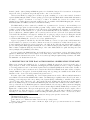
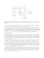
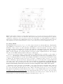
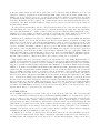
Observing with the Infrared Array Camera (IRAC) on the
Spitzer Space Telescope
Sean J. Careya , Mark Lacya , Seppo Lainea , William T. Reacha , Jason A. Suracea , William J.
Glaccuma , Joseph L. Horab , Steven P. Willnerb , Richard G. Arendtc , Matt L. N. Ashbyb , Lori
E. Allenb , Pauline Barmbyb , Bidushi Bhattacharyaa , Lynne K. Deutschb , Peter R. Eisenhardtd
, William F. Hoffmanne , J.-S. Huangb , Patrick J. Lowrancea , Massimo Marengob , S. Thomas
Megeathb , Brant O. Nelsona , Michael A. Pahreb , Brian M. Pattenb , Judith L. Pipherf , John R.
Stauffera , Daniel Sternd , Zhong Wangb , Gillian Wilsona , and Giovanni G. Faziob
a Spitzer
Science Center, MS 220-6, California Institute of Technology, Pasadena, CA 91125;
Center for Astrophysics, 60 Garden St., Cambridge, MA 02138-1516;
c Goddard Space Flight Center, Greenbelt, MD 2077;
d Jet Propulsion Laboratory, 4800 Oak Grove Dr., Pasadena, CA 91109;
e Steward Observatory, 933 N. Cherry Ave., Tucson, AZ 85721;
f Department of Physics and Astronomy, University of Rochester, Rochester, NY, 14627-0171
b Harvard-Smithsonian
ABSTRACT
We describe the astronomical observation template (AOT) for the Infrared Array Camera (IRAC) on the Spitzer
Space Telescope (formerly SIRTF, hereafter Spitzer). Commissioning of the AOTs was carried out in the first
three months of the Spitzer mission. Strategies for observing fixed and moving targets are described, along with
the performance of the AOT in flight. We also outline the operation of the IRAC data reduction pipeline at the
Spitzer Science Center (SSC), and describe residual effects in the data due to electronic and optical anomalies
in the instrument.
Keywords: telescopes, techniques: image processing, instrumentation: detectors, infrared: general
1. INTRODUCTION
1, 2
The Infrared Array Camera is one of the three science instruments comprising the payload of the Spitzer Space
Telescope.3 IRAC is a set of four imaging 256 × 256 pixel arrays with 50 × 50 fields of view and ∼1.00 2/pixel
platescales. The passbands are centered on 3.6, 4.5, 5.8 and 8.0 µm. The 3.6 and 4.5 µm arrays use InSb
detectors,4 the longer wavelength arrays are Si:As devices. Each array is read out by a set of four multiplexers,
each multiplexer reads out every 4th array column.
IRAC simultaneously images the sky in all four arrays using two fields of view whose centers are separated
by ∼6.8 arcmin. The 3.6 and 5.8 µm arrays share one field by means of a beamsplitter, and the 4.5 and 8.0 µm
arrays the other. IRAC has been designed to image the near- to mid-infrared sky from 3-9 µm with excellent
sensitivity and moderate resolution. It is extremely efficient at both very deep observations and shallow mapping
of large solid angles. Some representative science projects are infrared extragalactic source counts, 5 structure of
Galactic diffuse emission6 and detection and characterization of protostars in various star forming regions. 7, 8
The focal plane arrays image the sky by two sets of non-destructive reads, an initial set of pedestal reads
followed by a set of signal reads after the specified integration time. The difference of these two sets of reads
(known as Fowler samples) is then returned as the raw sky image in data numbers (DN). The data taking rate
of IRAC is ultimately limited by the 2s per raw image that it takes for data to be transferred from IRAC to the
spacecraft command and data handling processor (C&DH). IRAC observations consist of slewing the telescope
from one image position to the next and taking an image at each position. The telescope keeps an fixed inertial
Further author information: (Send correspondence to S.J.C.)
S.J.C.: E-mail: [email protected], Telephone: 1 626 395 8796
attitude (outside of jitter) during an IRAC integration for celestial fixed targets. For observations of solar system
targets, the telescope tracks the target throughout the course of an observation.
Observers use IRAC by creating an observation program containing one or more astronomical observation
requests (AORs) using the SPOT∗ software package provided by the SSC. Each AOR contains all the information
necessary to complete observations of one target or cluster. For IRAC, the observer chooses their desired
parameters (e.g. dither strategy, integration time) for the one available AOT, IRAC Mapping (the other two
instruments, IRS† and MIPS‡ each use several different AOTs).
The IRAC AOT provides a restricted yet flexible set of parameters for observers to use in tailoring a set
of observations appropriate for their scientific programs. Using a subset of all possible instrument parameters
permits a robust testing and calibration of the allowed modes and simplifies the designing of observations for
general observers. A less restrictive set of options would dramatically increase the amount of observatory time
spent on calibration, command uplink to the observatory, and resources needed for the development and testing
of the AOT. The AOT has been designed to facilitate the one pass proposal process used, reducing the amount
of support necessary for observers to plan useful observations. The AOT is designed to facilitate effective
observations while limiting the observer to choose less optimal strategies.
Approved programs are scheduled by the SSC. The AORs are converted to spacecraft readable instruction
sets and radiated to Spitzer for execution. Data from executed observations are radiated from Spitzer to the
ground, transferred from the Deep Space Network to the SSC. At the SSC, the raw data in units of DN are
processed through the IRAC pipelines resulting in a set of calibrated images (basic calibrated data or BCDs) in
units of surface brightness (MJy/sr), mosaic images of the entire AOR suitable for quick data inspection and
cursory analysis, and preliminary source lists§ .
Section 2 describes the IRAC AOT in some detail. In Section 3, we present an overview of the data reduction
pipeline for IRAC data and a brief description of the final data products. The data artifacts remaining in the
processed data are discussed in Section 4. Section 5 describes upcoming and planned improvements to the AOT.
We summarize our discussion in Section 6.
2. DESCRIPTION OF THE IRAC ASTRONOMICAL OBSERVATION TEMPLATE
This section describes the available modes of operation for IRAC. In general, an observer selects the type of
target, array mode, fields of view, frametime, and mapping and dither parameters. A more complete description
of observing parameters can be found in the Spitzer Observer’s Manual (SOM) at the SSC website. Details of
how to use SPOT to plan observations can be found in the SPOT User Manual at the same website. Complete
example AORs for some typical observations (shallow map and deep image) are available in the SOM. A brief
discussion of the observer selectable parameters is given in 2.1-2.5.
In terms of spacecraft commanding, the observer input parameters are used to fill in a standard instruction
set for IRAC observations. Each IRAC AOR consists of an initial target acquisition slew followed by the start of
tracking for a moving target and some pointing control system (PCS) commanding to switch from the attitude
observer¶ based control of motions to gyro only controlled motions. At this point, the array mode and integration
time for the IRAC arrays are set and the first IRAC integration is taken. The remainder of the AOR consists of
telescope slews followed by IRAC integrations consistent with the selected target, dither pattern and mapping
parameters. Offset slews can be done in either a reference frame aligned with the IRAC arrays or relative to the
Equatorial coordinate frame. The spacecraft queries the gyros to determine when the slew is complete, then a
delay is inserted to allow the telescope to settle before taking data. The settle time for IRAC observations is
currently 5 seconds. On the completion of all data taking, the PCS system is set back to observer based control.
∗
Spitzer Planning Observations Tool software, available from http://ssc.spitzer.caltech.edu.
The Infrared Spectrograph
‡
The Multi-band Imaging Photometer for Spitzer
§
Source lists are to be distributed in future versions of the processing software.
¶
In this context, attitude observer refers to the filtered output of the gyroscopes and star tracker used to determine
the spacecraft attitude.
†
Figure 1. An outline of the commanding for the IRAC AOT. The initialization of IRAC for each observation is done
concurrently with the initial acquisition slew. A more detailed description of the command sequences is beyond the scope
of this paper.
For long observations, the gyro based attitude is reset to the observer attitude approximately every 30 minutes
to reduce the effect of gyro drift. Figure 1 displays the logic of the IRAC AOT.
The IRAC AOT makes extensive use of onboard blocks (subroutines) to optimize efficiency and reduce the
number of instructions that need to be uploaded to the spacecraft. In addition, most adjustable parameters such
as dither patterns and settle time in the AOT are contained in instrument parameter files (IPPs) which can
be easily modified without code modifications and the lengthy processes of integration and testing. The IPPs
are modified at the discretion of the IRAC Instrument Support Team (IST) at the SSC to reflect our current
knowledge of on-orbit operations. Section 5 discusses some planned improvements to the IRAC AOT.
2.1. Target Modes
There are two main available target types, fixed and moving. Observations with all three science instruments,
IRAC, IRS and MIPS, share a common target architecture. Moving targets are solar system objects and are input
by either NAIF ID or name. The appropriate ephemeris is used to determine the necessary track parameters
for any date of observation. For newly discovered solar system objects, an ephemeris can be generated if orbital
elements are provided to the SSC. For fixed targets, the observer specifies the celestial coordinates and proper
motion, if any, of the target.
For each main target type, there is an option to have a cluster of targets. Often, it is advantageous to use an
offset cluster rather than multiple AORs as each AOR is charged an initial slew tax of 3 minutes. For a set of
short AORs of targets close to each other, the slew tax may account for the majority of the time charged to an
observer. All subtargets within the cluster must be within one degree of the main target. For moving targets,
the cluster targets are specified by offsets in arcseconds in either Equatorial coordinates or array coordinates.
The array coordinate option is useful for observers that would like to create their own custom dither pattern or
need to map a non-rectangular shape. The Equatorial option is useful for observers who want to make offsets in
some preferred direction (Ecliptic latitude, for instance).
Alternatively, fixed cluster targets may be specified by absolute positions rather than relative offsets; up to
100 subtargets may be used. This target mode is most useful for observing selected fields in an open star cluster
(e.g. Pleiades) or similar target. Fixed position cluster observations are slightly less efficient as the AOT does
not use the offset blocks implemented for relative cluster and non-cluster targets. Mapping observations are not
available for any cluster target observation.
Figure 2. The available parameter sets in the IRAC AOT. From top to bottom, the option types are main target mode,
cluster option, array mode, field of view, frametime, dither pattern, dither pattern scale and mapping mode. Only the
combinations of parameters connected by lines are allowed. It is important to note that mapping is not available for
cluster targets or in subarray mode. High dynamic range mode is only available for frametimes greater than 2s. If array
offset mapping is used and both full array fields of view are selected, then the special array mapping frame is used.
2.2. Array Modes
The IRAC AOT allows observers to choose one of three array readout modes, subarray, full array or high dynamic
range (HDR). For each array mode, there is a set of available fields of view (see the discussion in Sec. 2.3) and
frametimes. Only a subset of possible frametimes with IRAC are allowed in standard observations. This is
necessary as each specific frametime needs a dark offset calibration. Currently, the dark offset calibrations are
determined through a set of sky dark observations performed for each available frametime at least twice per
IRAC observing campaign. As a result, the skydark observations consume a significant fraction of the campaign
time allocated for IRAC calibrations (14% is allotted for calibrations).
Observers can specify the number of frames (framesets for HDR) that they would like for each pointing of
the telescope. We strongly recommend that only one frame(set) be taken for each pointing (with the
exception of using subarray mode for time series analysis). Well dithered observations are absolutely necessary
to mitigate the data artifacts described in Section 4. It may be tempting for many observers to use repeats
instead of dithering to increase the amount of integration time per total observation time (a typical dither and
settle takes ∼12 secondsk ), but those data will be less well calibrated. In particular, repeats will suffer from
a strong first frame effect (an array history dependent bias offset). In general, we recommend using the
longest nonsaturating frame time to increase on-source integration time rather than repeats.
Subarray mode uses a 20× faster clock (100 Hz) to read out the arrays and provides frame times of 0.02, 0.1
and 0.4 seconds. The entire array cannot be read out at the higher rate; therefore, subarray observations only
use a 32 by 32 pixel (the 8th through 39th row and column of each array) region near one corner of each array.
The platescale is unchanged from the full array scale so that a correspondingly smaller field of view is imaged.
64 samples are taken for each subarray frame (one subarray frame takes 1.28, 6.4 or 24.6 seconds, respectively
k
For the shortest full array frametime of 2s, the slew settle time between frames is used to transfer data. Repeats of
2s frames include a 5s delay between frames resulting in a maximum savings of only ∼ 7s.
at the three sample times); the raw data are packed into a 256 × 256 array, while the BCDs are 32 × 32 × 64
data cubes. Subarray observations are useful for imaging small, bright objects and extend the dynamic range of
IRAC to 20, 17, 63, and 45 Jy at 3.6, 4.5, 5.8, and 8.0 µm, respectively. Subarray observations are also useful
for analyzing rapidly varying phenomena (such as pulsars) and have been used to measure the spacecraft jitter
(0.100 rms). At this time, it is not possible to take continuous time series for any subarray frame time due to the
construction of the AOT. Observations will have delays of 1.72, 1.7 and 1.5 seconds between repeated 0.02, 0.1
and 0.4s subarray frames.
For the 0.1 and 0.4s frametimes, data are collected in all four arrays at once. The data from the arrays not
currently imaging the source on the subarray may be useful in subtracting the background. The data taking
rate of the 0.02s frametime is too high to permit collecting data in more than the channel imaging the source.
Mapping mode is not available for subarray observations, as mapping with such a small field of view is very
inefficient. If necessary, small maps could be made using a cluster offset target and subarray mode.
Full array mode, which uses a clock speed of 5 Hz, is the standard mode of operation for IRAC. The standard
frametimes available are 2, 12, 30, 100 and 200 seconds. For the 8.0 µm channel, observations are background
limited in 50 seconds; therefore, the 100s and 200s frametimes consist of 2 and 4 repeats respectively of 50s
frames. The 8 µm repeats are taken in a different fashion from user specified repeats in that they are internal
repeats to the IRAC data taking command as opposed to repeat calls of that command. As all 8 µm 100s and
200s data are collected in this fashion, the repeats are well calibrated in contrast to user specified repeats. For
deep integrations, observers should carefully consider if 200s or 100s frames are more appropriate. While the
200s frames will reach the confusion limit faster, they are more affected by radhits than the 100s frames and the
total number of useful pixels may be significantly reduced. The trade between the utility of 200s frames and the
amount of time necessary to calibrate them will be explored in the coming year of observations.
High dynamic range mode observations consist of sets of frametimes for each pointing. Each frametime set
consists of one long frametime observation which is preceded by a short and possibly an intermediate frametime.
HDR mode is designed for observations of regions containing both bright and faint sources where more dynamic
range is needed than is available using a single frame time. Examples of observations which benefit from using
HDR mode are studies of star formation in the Galactic plane and search for faint companions around moderately
bright stars. The long frametimes available in HDR mode are 12, 30, 100 and 200 seconds. The 12, 100 and
200 second HDR sets include an 0.6 second frame for the short frametime. The 0.6s frame has a maximum
unsaturated point source flux of 0.63, 0.65, 4.6 and 2.5 Jy for the 3.6, 4.5, 5.8 and 8.0 µm arrays. The 30s set
has a 1.2s short frame. The 100 and 200s HDR modes also include an intermediate frame time of 12s. HDR
mode observations are slightly longer than their full frame counterparts. The difference between the modes is
the time for the shorter frame integrations. As the shorter frames can transfer from IRAC to the C&DH while
the longer frames are being taken, HDR observations are 8%, 5%, 12% and 7% longer per pointing than their
full frame counterparts at 12, 30, 100 and 200s (assuming 1 frame set per pointing and 12s overhead for dither
and settle). The 200s HDR mode has not been used by observers and is likely to removed from service if not
requested in the first pool of general observer observations.
2.3. Fields of View
The four IRAC arrays image two separate fields of view on the sky at the same time. The observer has full
control over which fields of view image the target. For full array (including HDR mode) observations, the observer
can choose either or both of the 3.6/5.8 and 4.5/8.0 micron fields of view. For non-mapping observations and
mapping observations using celestial coordinates, if both fields are selected, then the target (or each separate
target in a cluster) is imaged for all dither positions in the 4.5/8.0 micron field of view and then is imaged for all
dithers in the 3.6/5.8 micron field of view. As the 3.6 micron field is most susceptable to long term latent images
(Sec. 4.2.4), that field of view is imaged on-target last so that the off-target data will be less contaminated.
Switching between fields of view costs one second per target; therefore, imaging of clusters instead of mapping
is slightly less efficient and is usually more cumbersome to plan.
If mapping mode in array coordinates is used, then the field of view used is centered halfway between the
3.6/5.8 and 4.5/8.0 micron fields of view. Figure 3 displays the relationship of this field of view with respect to
the IRAC arrays. The mapping field of view was created to perform efficient mapping of large regions and is
Figure 3. Relationship of the mapping frame to the IRAC fields of view. The AOR visualized (for a observation date of
24 June 2004) is a one row by one column map using the bright star (HR 5336) at the center of the image as the target.
The large squares show the placement of the IRAC fields of view. The small boxes show the placement of the subarray
fields of view. The subarray fields are labeled with the center wavelength of the array.
described in more detail in Sec. 2.4. However, for the smallest possible map, one row by one column, the target
will not be imaged on any array. Observers should use SPOT’s visualization tools for all observations
to make sure they are as intended.
The IRAC subarrays each have their own field of view (see Figure 3). To observe a target in all four arrays,
each field of view must be selected.
2.3.1. Rotation of FOVs
One aspect that observers have limited control over is the orientation of the fields of view with respect to celestial
coordinates. Due to thermal and power constraints, Spitzer must keep the axis perpendicular to the solar arrays
within a narrow range of angles toward the Sun. As a result, the sun to telescope boresight angle must be between
81 and 119 degrees and the roll of Spitzer about the boresight is constrained to ±2 ◦ . Then, the orientation of
the Spitzer focal plane on the sky is only a function of the date of observation and the Ecliptic latitude of the
target. Objects in the Ecliptic plane are only visible for about 40 days at a time and the orientation of the focal
plane rotates by 0.65◦ during this period. At the other extreme, the Ecliptic poles are continuously visible and
the focal plane orientation rotates 1◦ per day. Visualizing an AOR at the two ends and the middle of any one
visibility window will give a good idea of how the field orientation changes over all possible observation dates.
Figure 4 and Figure 5 display the changes in field of view orientation for a target in the Ecliptic plane and at
the Ecliptic pole.
Observations that absolutely need a particular aspect angle can be constrained as to the date of observation;
however, constraining the date of observation reduces both the chance that a program will be approved (there
is a cap on the percentage of awarded constrained observations in any proposal cycle) and that the observation
can be scheduled. In almost all circumstances, an observation of the required size and depth can be achieved by
using a slightly larger map and/or mapping in celestial coordinates.
2.4. Mapping
The IRAC AOT provides two options, array coordinate and celestial coordinate maps, for imaging regions larger
than 50 × 50 in size. For both map types, the observer specifies the number of map rows and columns and the
offsets in arcseconds between adjacent rows and columns.
Mapping in array coordinates ensures uniform coverage for any date of observation but leaves the orientation
of the map with respect to the celestial sphere unconstrained. For array coordinate maps, the field of view used
Figure 4. Variation of the field rotation for a target in the Ecliptic plane. This particular AOR is centered on 00 h 00m
00.s 00 +00◦ 000 00.000 . This target is only visible for ∼40 days at a time. The leftmost panel displays the field of view
orientation for 18 June 2004; the right panel displays the orientation for 25 July 2004. The amount of field rotation is
very small. The 3.6/5.8 µm FOV is the large dark grey square surrounded by two smaller boxes representing the stray
light producing regions. The 4.5/8.0 µm field of view is the large light grey square; it has three associated stray light
boxes.
is the mapping FOV which is centered on the spot midway between the 3.6/5.8 and 4.5/8.0 µm FOVs. The row
direction is along the axis connecting the 3.6/5.8 and 4.5/8.0 micron arrays. To ensure that both fields of view
image the target region, maps usually have more rows than columns. Array mapping works well for mapping
large regions that are roughly square in aspect ratio. For elongated objects, array coordinate maps can be
inefficient as a much larger region may need to be mapped to ensure coverage for all possible array orientations.
This is true in particular for targets at high Ecliptic latitude.
The second mapping option, celestial coordinate maps is useful for mapping elongated objects. In addition to
the number of rows and columns, and grid spacing in row and column, the observer specifies a map orientation
(in degrees East of North) for determining the positioning of the map grid centers. A suitable choice of map
angle may greatly reduce the number of map points needed to cover an elongated object. While the observer can
control the placement of the map points, the orientation of the arrays on the sky is still controlled by the date of
observation. Unless the map uses a finely spaced grid, gaps in coverage are possible for some observation dates.
In addition, the coverage of celestial maps will be non-uniform with the coverage at the map edges being highly
date dependent. We do not advise the use of celestial mapping except for mapping elongated objects and highly
recommend that the observer visualize the map over the full range of observing dates. Celestial coordinate maps
will execute the map in each selected field, the special mapping field of view is not used.
2.5. Dithering
The IRAC AOT provides a comprehensive set of predefined dither patterns for the observer to use for full array
observations. Dithering is highly desirable for any observation; properly dithered observations will mitigate the
effects of bad pixels and pixel to pixel errors in the flatfield. Dithering also benefits in radhit rejection and the
removal of latent images and scattered light. The SSC mosaicer obtains satisfactory radhit rejection with four
dithers and excellent rejection with five or more dithers. Three dithers is the absolute minimum recommended
redundancy. All of the predefined IRAC dither patterns incorporate sub-pixel dithering to improve sampling in
mosaics using drizzle or other reconstruction techniques. For both the full array and subarray modes, there are
three dither scales, small, medium and large. The scaling of the dither patterns is roughly 1:2:4. The medium and
large dither scales are recommended for most observations, the small dither scale is most useful when mapping
with fractional array offsets.
Figure 5. Variation of the field rotation for the North Ecliptic Pole which is continuously visible by Spitzer. The fields
of view are as identified in Figure 4. The leftmost panel is the orientation of the IRAC fields of view on 01 June 2004, the
middle panel displays the orientation of the FOVs on 01 September 2004 and the rightmost panel displays the orientation
on 01 December 2004.
A variety of dither patterns are available in full array mode, 12 and 36 point Reuleaux triangle, 5 point
Gaussian, 9 point random (points drawn from a uniform distribution), 16 point spiral and cycling. The spiral
pattern was designed for IRAC to be compact but also have a good figure of merit 9 for self-calibration. The
Reuleaux patterns are also well suited for observers who are considering self-calibrating their images ∗∗ . The
random and spiral patterns are the optimum size for 1/3 and 1/4 subpixel dithering. The cycling dither pattern
allows observers to specify a pattern of any desired depth. The pattern has 311 independent positions with each
set of four consecutive dithers providing complete 1/2 pixel sampling. When used with mapping, the cycling
dither pattern will provide a different dither position for each map center even if the dither pattern has a depth
of one. The subarray mode has only two options, a four point pattern drawn from a Gaussian distribution and
a nine point Reuleaux triangle.
3. OVERVIEW OF DATA REDUCTION PIPELINE
The IRAC pipeline at the SSC produces two sets of data products from the raw data. The basic calibrated data
(BCDs) are the raw data frames processed for bias (dark) offsets, pixel to pixel gain variations, nonlinearity and
other instrumental signatures. Section 3.1 describes the data products derived from the BCDs. A more complete
description of the IRAC pipeline is available in the IRAC Pipeline Description Document available at the SSC
website. A separate processing pipeline, SIP10 , was created by the IRAC instrument team†† . While SIP uses
the same algorithms as the official IRAC pipeline, it was written independently and is used for validation and
code development purposes.
Three of the pipeline operations, dark offset subtraction, flat fielding and absolute calibration, require inputs
derived from on-orbit calibration observations which are conducted every IRAC observing campaign. The dark
offset is derived from well dithered observations of a low background (high Ecliptic latitude) region for each
frametime. The dark data are median stacked with outlier rejection and object masking to create dark frames.
The flat fields are also derived from sky data; in this case, well dithered 100s frametimes of the Zodiacal light
are used to generate the flatfield. Science observations are processed with the flat field and dark frame that are
nearest in time to the observation and validated by the IRAC IST. The flux calibration for IRAC is derived from
observations of ten primary calibrators at the beginning and end of each campaign. A scaling factor between
DN/s and MJy/sr for each IRAC channel is determined by comparing the measured flux of each calibrator with
∗∗
The SSC does not currently support the self-calibration method of data reduction.
The instrument team at the Smithsonian Astrophysical Observatory oversaw the design and development of IRAC,
which was built at NASA Goddard Space Flight Center. Responsibility for the day to day operation of IRAC transferred
to the IRAC instrument support team (IST) at the SSC at the end of the in-orbit checkout. The teams continue to work
collaboratively to improve the performance of the instrument.
††
flux estimates of the standards derived from spectral templates. The stability of the calibration is monitored by
observing a network of secondary standards every twelve hours. The secondary calibrators are in the Ecliptic
plane and are paired with Spitzer downlinks to improve scheduling efficiency. It is likely that the amount of
time allocated to IRAC calibrations (currently 14% of the total IRAC campaign) will be reduced due to the high
degree of stability that IRAC displays.
The BCDs are absolutely calibrated in units of surface brightness (MJy/sr). The BCDs are FITS files
consisting of the calibrated data for one (64 for subarray mode) image per IRAC array. Each BCD has a header
consisting of useful instrument telemetry pertaining to the data collection, astrometry assembled from the PCS
telemetry and keywords that can be used to trace the calibrations applied to the image data. Complete details
of the BCD headers are available in the IRAC Data Handbook.
3.1. Post-BCD Pipeline
The second set of data products are the browse quality data (BQDs). The BQDs consist of mosaics of the BCDs
from each IRAC channel and source lists in each band. Radhit detection, artifact masking and astrometric
refinement are performed on the input BCDs before mosaicing and extracting sources from the image stack.
Recently, a tool has been developed which will allow the observer to estimate a point response function (PRF)
directly from their data if the published PRFs are not sufficient. The mosaicer, source extractor and PRF
estimator are publically available through the SSC website. For the current generation of the post-BCD pipeline,
only the automated mosaics are valid; therefore, the source lists are not distributed at present.
4. DISCUSSION OF DATA QUALITY AND ARTIFACTS
A variety of data artifacts remain in the pipeline processed IRAC images. Most of the artifacts are related to
or are enhanced by bright sources; that is, sources for which the fluence is a significant fraction of the detector
well depth. The residual artifacts are both electronic and/or optical in nature. The SSC is currently developing
corrective algorithms for most of the artifacts. It is hoped that tools will be provided to the user community to
correct the BCDs for some of the artifacts by the end of 2004. Modifications to the SSC pipeline will happen
at a slower pace due to the stringent testing and version control required for operations software. Many of the
artifacts can be mitigated by well designed observations. Most of the optical artifacts can be masked in well
dithered observations. Using HDR mode, the short frames will provide some data which is not affected by the
electronic artifacts produced by bright sources.
4.1. Photometric Stability
To date, the on-orbit stability of IRAC is excellent. The measured temporal variation in the flat field is < 2%.
The repeatability of the measured flux for any given calibrator is 1-2% and 2-3% for the flux scaling derived
from the network of calibration stars. We conservatively estimate the absolute calibration to be good to 10%.
4.2. Electronic Artifacts
Electronic artifacts include saturation, latent images, multiplexer bleed (muxbleed), and column pulldown. Well
dithered observations will be robust against latent images. Muxbleed and column pulldown are functions of the
source fluence. Figure 6 displays examples of muxbleed and column pulldown. Using HDR mode for observations
of bright source fields will provide some data for the affected regions.
4.2.1. Saturation
Saturated pixels manifest themselves in IRAC data in two ways. Pixels which saturate in the signal reads of the
Fowler sampling will have DN values & 40000. These pixels are flagged by the BCD pipeline. More insidious are
pixels which saturate in the pedestal reads. These pixels have resulting values of . 2000 DN and are difficult to
differentiate from unsaturated data. The pedestal saturated pixels are always due to sources of very high fluence
and produce holes in the observed PSFs of the brightest sources. The holes can be easily corrected in HDR data
by replacing the saturated pixels with the corresponding short frame pixels. Very recently, a more general tool
for detecting holes in all BCD data has been created.
Figure 6. Examples of muxbleed and column pulldown in a 12s frame at 3.6 µm. Several columns containing bright stars
have different levels of pulldown in this image. The most obvious example of muxbleed is the trail of pixels to the right
of the bright star on the left hand side of the image.
4.2.2. Muxbleed
Two effects cause a bright source to leave artifacts that stretch along the readout direction. The time constant
for the readout amplifiers is somewhat longer than the readout time for a pixel; this bandwidth effect causes the
subsequent readouts after a bright source to have an excess signal. A similar, but not well understood, effect in
the multiplexer causes a longer-duration memory. Figure 6 shows an image with a bright source. The trail of
dots following the bright source along the readout direction (horizontal, with readout from left to right) wrap
around to the next row. The SSC pipeline has a correction for both the finite response (which affects all arrays)
and muxbleed (which only affects the 3.6 and 4.5 µm arrays); however, the correction still leaves significant
residuals. Once again, HDR mode observations are of some utility in determining the true sky level for pixels
affected by muxbleed.
4.2.3. Column Pulldown
Sources of a large enough fluence cause the level of the column containing the source to be depressed. A standalone
IDL routine is available to remove column pulldown for images with little extended emission. In addition, the
SSC is providing a cosmetic correction algorithm for both muxbleed and column pulldown. Observers should be
cautious when interpreting data that has been cosmetically corrected. An analogous effect exists along rows for
the 5.8 and 8.0 µm arrays.
4.2.4. Latent Images
All IRAC arrays have some degree of image latents. Extremely long term latents can be generated for the 3.6
and 8.0 µm arrays. These arrays are annealed following downlinks (every 12 hours) to remove the long term
latents. The long term latents can affect the observations of subsequent observers. The SSC schedules the most
likely latent producing observations immediately prior to downlinks to reduce their effect on other programs.
The SSC pipeline flags pixels containing latents produced in each AOR. The flagging does not presently extend
from one AOR to the next. Well dithered observations are fairly resistant to latent images (including long term
latents).
4.3. Optical Artifacts
Optical artifacts include stray light from bright sources off the array, ghost images due to internal reflections in
the filters and beamsplitters and, for the 5.8 and 8.0 µm arrays, internally scattered light. Figure 7 shows stray
light and ghost image examples.
Figure 7. Examples of stray light and a ghost image in a 12 second frame from an AOR (AOR request key 0004958976)
in the Galactic First Look Survey at 3.6 µm. The left panel shows one dither position without stray light for reference.
The middle panel is the next dither position. A patch of stray light is evident in the upper right hand corner of the image;
the star causing the stray light is above and to the right of the array. In the rightmost panel, we zoom in to the top of
the image which is now displayed with a logarithmic stretch. An example of a ghost image is the circle above and to the
left of the bright star.
4.3.1. Stray Light
The 3.6 and 4.5 µm arrays each have significant regions slightly off the array which produce stray light spots
with peak brightnesses ∼0.2% of the source creating the light. The regions causing stray light can be displayed
by SPOT when designing observations. Observations which have dithers larger than the stray light regions can
remove stray light through judicious masking. A post-BCD tool to mask stray light is currently in development.
4.3.2. Ghost Images
The most significant ghost images are produced by internal reflections in the filters for each array. The 3.6 and
4.5 µm ghosts are approximately 0.05% of the peak intensity of the source. The location of these ghosts relative
to the source is dependent on the source position on the focal plane. Once again, using large dithers can help
mitigate the 3.6 and 4.5 µm ghosts. The 5.8 and 8.0 µm ghosts are smaller, but the ghosts are in fixed positions
with respect to the source; therefore, dithering will not remove the long wavelength ghosts.
4.3.3. Internally scattered light
Analysis of on-orbit data has shown that a significant fraction of the light entering a pixel for the 5.8 and 8.0
µm arrays is internally scattered throughout the array. Some of the scattered light is concentrated along the row
and column containing the pixel, with the remainder scattered more uniformily throughout the array. The exact
mechanism of the scattering is currently being characterized using test arrays on the ground. The scattered light
produces artifacts in row and column that need correction. Empirical corrections similar to the column pulldown
correction are currently being designed. In addition, the more diffuse component of the scattered light causes
the response of the arrays to point and extended sources to be different. As the BCDs are calibrated using point
sources, fluxes of extended sources, with diameters > 80 arcsecond (such as the Zodiacal background), need to
be scaled by 0.63 and 0.69 for the 5.8 and 8.0 µm arrays, respectively.
5. FUTURE DIRECTIONS
Improvement and optimization of both the IRAC AOT and the IRAC data reduction pipelines are ongoing. As
we continue to characterize the flight data and better understand the remaining image artifacts, improvements
to the pipeline will be developed. The masking of stray light from point sources is one planned upgrade to the
pipeline. Developing algorithms to correct column pulldown and some of the optical banding are high priorities
of the IRAC instrument (SAO) and instrument support teams (SSC). Based on on-orbit data, the use of the
pointing control system during IRAC observations has already been optimized to improve stability during long
integrations and reduce the settle time for the initial acquisition slew.
5.1. AOT Improvements
Several upgrades to the IRAC AOT are planned for use in the next general call for proposals (proposals for
general observer cycle 2 will be due in Feb 2005). The first set of upgrades are to the commanding and slew
efficiency in the IRAC AOT. The most significant of these improvements will reduce the wall clock time for an
observation by 2-10%. A second change to implement a settle time which is dependent on slew length will reduce
the time needed for most well-dithered observations.
Two additional options to AOT are planned for the coming year. The first is the ability to take a continuous
time series of data in subarray mode. This option will be available for the 0.1 and 0.4s frametimes. This mode is
intended for observers who wish to monitor very short period, time variable sources. The second new mode will
provide sets of channel dependent frametimes with one or more shorter frames taken at 3.6 and 4.5 µm per single
longer frame at 5.8 and 8.0 µm. The multi-frametime option is designed for observations of sources with star-like
spectral energy distributions (Sν ∝ ν 2 ). Currently, stars can saturate in the short wavelength arrays without
producing high signal-to-noise in the longer wavelength arrays. Sets of useful frametimes will be developed and
made available for use. Prototypes of this option are currently used for the observations of our primary and
secondary calibration stars.
6. SUMMARY
The IRAC Astronomical Observation Template provides a set of limited but flexible set of instrument and
observatory parameters for observers to use in the design of their observations. Observers should plan welldithered observations to mitigate a variety of optical and electronic data artifacts. Work is continuing on
improving both the IRAC AOT and the IRAC data pipeline.
ACKNOWLEDGMENTS
This work is based on observations made with the Spitzer Space Telescope, which is operated by the Jet Propulsion Laboratory, California Institute of Technology under NASA contract 1407. Support for this work was
provided by NASA through an award issued by JPL/Caltech.
REFERENCES
1. G. G. Fazio et al., “In-flight performance of the Infrared Array Camera on the Spitzer Space Telescope,”
Astrophys.J.Suppl. in press, 2004.
2. J. Hora et al., “In-flight performance and calibration of the Infrared Array Camera (IRAC) for SIRTF,”
this volume .
3. M. W. Werner et al., “The Spitzer Space Telescope,” Astrophys.J.Suppl. in press, 2004.
4. J. L. Pipher et al., “Comparison of laboratory and in-flight performance of the InfraRed Array Camera
(IRAC) detector arrays on the Spitzer Space Telescope,” this volume .
5. G. G. Fazio et al., “Number counts at 3 < λ < 10 microns from the Spitzer Space Telescope,” Astrophys.J.Suppl. in press, 2004.
6. “Structure and colors of diffuse emission in the Spitzer Galactic First Look Survey,” Astrophys.J.Suppl. in
press, 2004.
7. W. T. Reach et al., “Protostars in the elephant trunk nebula,” Astrophys.J.Suppl. in press, 2004.
8. A. P. Marston et al., “DR21: A major star formation site revealed by Spitzer,” Astrophys.J.Suppl. in press,
2004.
9. R. G. Arendt, D. J. Fixsen, and S. H. Moseley, “Dithering strategies for efficient self-calibration of imaging
arrays,” Astrophys. J. 536, pp. 500–512, 2000.
10. P. Barmby, Z. Wang, M. Marengo, and M. L. N. Ashby, “SIP: a modern, flexible data pipeline,” this volume
.