Download Manual - UTAM - University of Utah

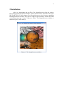
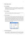
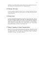
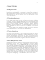
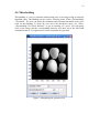
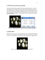
Image Processor
User Manual
Edition 1.0
Chaiwoot Boonyasiriwat and Julie Willis
University of Utah
February 23, 2006
2
First Edition, February 2006 (2/23/2006)
Published by UTAM.
Email: [email protected], [email protected]
Online version of this manual is available at
http://utam.gg.utah.edu/chaiwoot/improc
If you found any problems with this manual, please notify us at the above email
addresses.
Copyright © University of Utah 2006
Permission is granted to copy and distribute this document. If you would like to
modify this document, please contact us and ask for permission.
3
Table of Contents
Preface………………………………………………………………….. 5
1 System Requirements………………………………………………... 7
1.1 Hardware Requirements……………………………………………………… 7
1.2 Software Requirements………………………………………………………. 7
2 Installation……………………………………………………………. 8
3 Basic Operations……………………………………………………... 9
3.1 Load images………………………………………………………………….. 9
3.2 Save images…………………………………………………………………... 9
3.3 Resize images………………………………………………………………… 9
3.4 Measure distances…………………………………………………………….. 9
3.5 Change colormap……………………………………………………………..10
3.6 Zoom in/out………………………………………………………………….. 10
3.7 Image cropping……………………………………………………………….10
4 Image Filtering……………………………………………………… 11
4.1 Edge detections……………………………………………………………... 11
4.2 Intensity adjustments……………………………………………………….. 11
4.3 Noise eliminations………………………………………………………….. 11
4.4 Morphological operations…………………………………………………... 11
4.5 Thresholding…………………………………………………………………12
5 Image Segmentation……………………………………………….. 13
5.1 Watershed transform……………………………………………………….. 13
5.2 Modified watershed transform………………………………………………13
5.3 ROCK segmentation algorithm…………………………………………….. 14
5.4 BWLABEL………………………………………………………………….14
6 Label Handling……………………………………………………... 15
6.1 Load label…………………………………………………………………… 15
6.2 Save label…………………………………………………………………… 15
6.3 Add label…………………………………………………………………… 15
6.4 Delete label…………………………………………………………………. 15
6.5 Merge label…………………………………………………………………. 15
6.6 Remove holes in labels………………………………………………………15
6.7 Show label number…………………………………………………………..15
6.8 Show label statistics………………………………………………………… 15
7 Statistical Analyses…………………………………………………. 16
7.1 Show a pair of statistics…………………………………………………….. 16
7.2 Export statistics………………………………………………………………16
7.3 Draw and remove regions of interest……………………………………...... 16
4
8 Global Images – A way to handle large images…………………… 17
8.1 Set global image…………………………………………………………….. 17
8.2 Set working image window size…………………………………………….. 17
8.3 Set working image…………………………………………………………... 17
8.4 Operations of global image…………………………………………………. 17
8.5 View global image………………………………………………………….. 17
8.6 View working image………………………………………………………... 17
References………………………………………………………………18
5
Preface
This manual contains the system requirements, the instructions for
installation, and the use of the ImageProcessor.
The ImageProcessor was funded by the University of Utah. It is a
MATLAB-based, image-processing toolbox originally designed for
segmenting rocks from digital images of sediments. Now we are trying to
apply it to some other applications as many as we can.
We wish you found it useful for your applications. We would
greatly appreciate if you send us comments, suggestions, bug reports, and
potential applications.
Chaiwoot Boonyasiriwat
February 23, 2005
6
7
1 System Requirements
To use the ImageProcessor, the user should have a system that satisfies the
following requirements.
1.1 Hardware Requirements
•
•
•
CPU: Intel Pentium III 800 MHz or higher, AMD Athlon 800 MHz or higher
Memory: 256 Mbytes (512 Mbytes is recommended)
Hard drive: 10 Mbytes
1.2 Software Requirements
•
•
Mathworks MATLAB version 6.0 or higher
Mathworks Image Processing Toolbox
8
2 Installation
After you downloaded the zip file of the ImageProcessor from the website
http://utam.gg.utah.edu/chaiwoot/improc, please extract it into a local disk. Then open
MATLAB. In MATLAB, change your current directory to the directory containing
the ImageProcessor toolbox. Now you are ready to run the toolbox. In the MATLAB
command prompt, type “improc” and press “Enter”. The ImageProcessor window as
shown in Figure 1 will show up.
Figure 1. The ImageProcessor window.
9
3 Basic Operations
3.1 Load images
ImageProcessor can load images in two ways. The first one is to use menu “File>Load Image File”. This menu is used to load regular images in the formats: JPG,
PNG, BMP, TIF. The other way is to use menu “File->Load MAT File”. This is
used to load a MAT containing an image I.
3.2 Save images
Once the user has loaded an image into ImageProcessor, the image can be saved
into a MAT file by using menu “File->Save Image As MAT File”.
3.3 Resize images
The user can resize an image by using menu “Image->Resize Image”. Once the
user selects the menu, the Resize Image window will show up as shown in Figure
2. To reserve the image scale (width per height), once the user changes the image
width, the image height will be automatically changed. There are three methods of
resizing an image: nearest neighbor, bilinear and bicubic. After all parameters
have been set, click the “Apply” button to resize the image. If the user does not
satisfy with the resized image, click the “Restore” button to restore the image to
its original size. To close the window, either click the “Close” button or the “X”
icon at the top right of the window.
Figure 2. Resize Image window.
3.4 Measure distances
The user can measure a distance between two points by using menu “Image>Measure Distance”. To start the measurement, click on the image to define the
starting point and then click again to define the end point. The measured distance
10
will show up in the MATLAB command window. The user can repeat this process
until satisfied. To terminate this process, use right-mouse click.
3.5 Change color map
To user the image color map, user menu “View->Colormap” and choose any type
of color map. The available color maps are bone, cool, copper, flag, gray, hot, hsv,
jet, pink, and prism.
3.6 Zoom in/out
To turn on the zooming functionality, use menu “View->Zoom->On”. The user
can zoom the image by clicking on the image. The clicked point will be used as
the center of zooming. Another way to zoom is to click and drag to define the
region to be zoomed in. The user can choose to zoom only in the horizontal or
vertical direction by using menu “View->Zoom->XOn” or “View->Zoom->
YOn”, respectively. To zoom out, use menu “View->Zoom->Out”. To turn off the
zooming functionality, use menu “View->Zoom->Off”.
3.7 Image Cropping (or Image Fragmentation)
Image crop is a way to cut off uninteresting parts of an image. ImageProcessor has
two ways to crop an image. The first one is a rectangular crop and the second one
is a polygon crop. To use an image crop, select menu “Image->Crop Image>Rectangle” or “Image->Crop Image->Polygon”.
11
4 Image Filtering
4.1 Edge detections
ImageProcessor provides an ability to detect edges in an image. There are 6 types of
edge detectors available for the user: Canny, Laplacian of Gaussian, Prewitt, Roberts,
Sobel, and Zero-Cross. The user can select one of these edge detectors in menu
“Filter->Edge Detection”.
4.2 Intensity adjustments
In some images, image contrast is not very good due to a lot of reasons, e.g. lighting
environment. The user can adjust and enhance the image contrast or intensity using,
e.g., histogram equalization. ImageProcessor provides the user some filters: Brighten,
Darken, Contrast Mapping, Histogram Equalization, Adaptive Histogram
Equalization, Histogram Normalization, Non-uniform Illumination Correction, and
Image Complement. These filters can be accessed by using menu “Filter->Intensity
Adjustment”.
In some images, the user has to invert the image intensity before applying an
image segmentation filter, e.g., ROCKS filter for segmenting rocks.
4.3 Noise eliminations
Some images contain noises which are undesirable for later processing steps. The user
can kill these noises by using a median filter, a uniform smoothing filter, or an edgepreserving smoothing filter. ImageProcessor has various types of filters for this
purpose including 2D Median Filter, Uniform Smoothing Filter, and Edge Preserving
Filter. These filters can be accessed by using menu “Filter->Noise Elimination”.
4.4 Morphological operations
Morphological operations are operations for analysis of spatial structures in an image.
ImageProcessor provides various types of morphological operations: Dilation,
Erosion, Opening, Closing, Top-Hat, and Bottom-Hat. The user can use this feature
using menu “Filter->Morphological Operations” as shown in Figure 3. The user can
choose a type of morphological operation in the “Operation” drop box and choose a
type of structuring element (STREL) in the “Structuring Element” drop box. The size
of the structuring element can be assigned in the text box next to the drop box. Once
all of parameters are set, click the “Apply” button and the result will be displayed in
the same window. If the user is satisfied with the result, click the “Update” button to
update the working image. If the user does not click the “Update” button, there will be
no change in the working image. To close the window, click the “Close” button.
12
4.5 Thresholding
Thresholding is a way to eliminate uninteresting parts of an image using an intensity
threshold value. Thresholding can be used by selecting menu “Filter->Thresholding>Threshold”. The user can define the minimum and maximum threshold values to be
used for thresholding. To help the user select the threshold values, use “Filter>Thresholding->Get Pixel Intensity” to get an intensity of a pixel. Use left-mouse
click on the image and the corresponding intensity will show up in the MATLAB
command window. Use right-mouse click to terminate the operation.
Figure 3. Morphological operation GUI.
13
5 Image Segmentation
5.1 Watershed transform
Watershed transform is an algorithm for image segmentation. To use this feature,
select “Segmentation->Watershed Transform”. Figure 4 shows a segmentation result
using the watershed transform. As you can see from the result, the watershed
transform produced an over-segmented result.
Figure 4. Image segmentation using the watershed transform.
5.2 Modified watershed transform
The modified watershed transform is an improved version of the watershed transform.
The idea is to enhance the input image before applying the watershed transform. The
improvement is done by using top-hat and bottom-hat filters to enhance the mountains
and valleys in the image. Then an H-minima transform is applied to eliminate some
potholes. A segmentation result using the modified watershed transform is shown in
Figure 5. To use this feature, select “Segmentation->Modified Watershed Transform”.
Figure 5. (Left) Image segmentation obtained using the modified watershed
transform. (Right) Parameters used in the modified watershed transform.
14
5.3 ROCKS segmentation algorithm
The ROCKS segmentation algorithm was developed by Boonyasiriwat et. al (2006).
This algorithm was originally designed for segmenting clasts (fragments of rocks)
from digital images of a mega-trench in Mapleton, Utah. The ROCKS algorithm is an
improved version of the modified watershed transform. The improvement is done by
using thresholding, and various morphological operations. To use this feature, select
menu “Segmentation->ROCKS”. A segmentation result using the ROCKS algorithm
is shown in Figure 6.
Figure 6. (Left) Image segmentation obtained by using the ROCK segmentation
algorithm. (Right) Parameters used in the ROCK segmentation algorithm.
5.4 BWLABEL
BWLABEL stands for bit-wise labeling algorithm. Before applying BWLABEL, the
user has to use thresholding to eliminate uninteresting parts of the image so that they
become zero in the image. To use this feature, select “Segmentation->BWLABEL”.
Figure 7. Image segmentation obtained by using BWLABEL.
15
6 Label Handling
6.1 Load label
6.2 Save label
6.3 Add label
6.4 Delete label
6.5 Merge label
6.6 Remove holes in labels
6.7 Show label number
6.8 Show label statistics
16
7 Statistical Analyses
7.1 Show a pair of statistics
7.2 Export statistics
7.3 Draw and remove regions of interest
17
8 Global Images – a way to handle large images
8.1 Set global image
8.2 Set working image window size
8.3 Set working image
8.4 Operations of global image
8.5 View global image
8.6 View working image
18
References
Boonyasiriwat, C., Willis, J., Schuster, G.T., and Brunh, R., 2006: “ROCKS
Segmentation Algorithm for Optical Stratigraphy”, in preparation.
Boonyasiriwat, C., Willis, J., Schuster, G.T., and Brunh, R., 2006: “ImageProcessor:
A Tool for Optical Stratigraphy”, in preparation.
Willis, J., Boonyasiriwat, C., Brunh, R., and Schuster, G.T., 2006: “Applications of
Optical Stratigraphy”, in preparation.