Download General introduction

Introduction to Data Exploration and Visualization1
Introductory remarks: The handout series are collections of (1) illustrative examples shown and
discussed during the formal presentation, meant to be annotated (i.e. not always self-explanatory) (2)
information on how to use the EDA software (3) additional examples and implicitely or explicitely
suggested directions for your exploration, (4) background information ...
Example collection
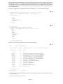
Ex.1
26 cantons
Stemleaf:ALPS(1) Initiative of the Alps (rail transit)
Legend: 2|6 stands for 25.51;
8|8 for 87.54
2|6
3|668
4|458
5|122355567799
6|000124
7|
8|8
Ex.2
183 countries
Stemleaf:Pop93(3) Population 1993
Legend: 0|0 stands for 2000.00; 11|9 for 1188628990.00
0|0000000000000000000000000000000000000+138
1|2236
2|06
3|
4|
5|
6|
7|
8|
9|0
10|
11|9
Ex.3
Stemleaf:Pop93(3) Population 1993
Legend: 0|0 stands for 2000.00; 34|2 for 35212000.00
0|0000000001111111111111222222222233344+27
2|144456789123335557
4|0113356601122369
6|26955778
8|5566779017899
10|1457934
12|007
14|0028
16|5688
18|294
20|16112
22|736
24|
26|1334
28|79
30|
32|4
34|2
hi |(*27)
_______________________________________________________________________________________________________________________
1. E. Horber, 13.12.98 : intro.mss
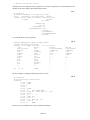
This example shows the default display for the same data shown in the previous example. Observations
much bigger (or smaller) - relatively speaking - than the others appear on a separate high (labelled hi) or
low (labelled lo) stem. As a principle these observations should be identified and named. In this case there
is not enough room to do so on a single stem-line, therefore EDA simply informs you that there are 27
countries on that stem.2
In the next example there is enough room to show case identifiers3, i.e. Swiss canton abreviations.
Ex.4
Stemleaf:ALPS(1) Initiative of the Alps (rail transit)
Legend: 3|8 stands for 37.65;
6|4 for 63.78
lo |VS FR VD
3|8
4|458
5|122355567799
6|000124
hi |UR
Ex.5
30 countries
Stemleaf:PGrow(4) Population Growth
Legend: -4|0 stands for -0.30; 10|0 for 1.10
-4|
-2|00
-0|0
0|000
2|00000000
4|00000
6|000
8|00
10|000
hi |ALBA TURQ AND
Below you will find a stem-and-leaf plot as it is produced by SPSS.
Ex.6
AGE
Age of respondent
Valid cases:
959.0
Frequency
Stem &
2.00
98.00
108.00
100.00
97.00
97.00
99.00
63.00
77.00
40.00
53.00
35.00
56.00
33.00
1.00
1
2
2
3
3
4
4
5
5
6
6
7
7
8
8
Stem width:
Each leaf:
.
*
.
*
.
*
.
*
.
*
.
*
.
*
.
Missing cases:
2.0
Percent missing:
.2
Leaf
&
000000011111112222222333333344444
55555555556666667777788888889999999
000000000011112222233333444444444
55555555666667777778888888999999
00000011111111222222333334444444
555555555566666677777888888999999
000011111222233333444
55566666777788888889999999
00011122233344
555666777888889999
000122233444
5556666777888888999
0001122344
&
10
3 case(s)
_______________________________________________________________________________________________________________________
2. The parentheses and the star are used to signal that this is the count of observations on the stem and not some - strangely labelled- observation or
a stem containing digit-leaves.
3. In the EDA Software these names are called CASIDs
-EDA 1.2 -
& denotes fractional leaves.
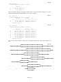
Stemleaf-plots can be adapted for other purposes, for instance comparison of the distributions of two
variables on the same display, showing them back to back.
Ex.7
30 countries
Stemleaf:LifeEM(6) Life Expectancy (men)
with
:LifeEF(7) Life Expectancy (women)
Legend: 68|0 stands for 68.00; 82|0 for 83.00
LifeEM
LifeEF
|lo |TURQ
000000|
00|
000000000|
0000000000000|
|
|
|
|
68|
70|
72|
74|0
76|0000
78|00000000
80|000000000000
82|0000
or to study differences between groups...
Ex.8
Stemleaf:GNPAgr(20) %GNP for Agriculture
Groups defined by Continents
Legend: 0|0 stands for 0.00;
5|5 for
Asia
Africa
0|0111112234
|34
0|55778
|55567
1|01
|1224444
1|6899
|566
2|123
|111112
2|5567
|577
3|24
|011344
3|9
|567
4|12
|3444
4|
|5555677
5|11
|01123
5|
|5
hi
|(* 4)
|GNEQ
55.00
Europe
|1123333334444
|55666788
|134
|667
|03
|
|3
|
|
|
|
|
N&C.Am
|1122233444
|5667899
|134
|666999
|124
|
|03
|
|
|
|
|
|
|
The next example is a histogram showing case ids as “leaves”.
Ex.9
30 countries
Histogram:Urb(5) Urbanization
midpoint
32.50 | PORT
37.50 | ALBA
42.50 |
47.50 |
52.50 | ROUM
57.50 | A
IRLA GREC HNGR
62.50 | TURQ CH
POLO CHYP FI
67.50 | BULG
72.50 | N
I
F
77.50 | TCHE LUX
82.50 | LIE S
87.50 | DK
MALT UK
NL
92.50 | ISLA D
E
97.50 | B
MONA
AND
The next series of examples shows various numerical summaries
-EDA 1.3 -
Ex.10
183 countries
Summary:GNPCap(19) GNP per capita
H
O
1622.00
+-------------------+
|
479.50 6491.50 |
|
71.00 50000.00 |
This is a 5-number summary showing the median (1622), as well as the hinges labelled “H” (=letter
value) and the minimum/maximum labelled “O” for “One” (=depth 1).
Ex.11
183 countries
Summary:GNPCap(19) GNP per capita
1622.00
spread
mid
+---------------------------------------+
H |
479.50 6491.50 | 6012.00 3485.50 |
O |
71.00 50000.00 | 49929.00 25035.50 |
Trimean= 2553.75
Ex.12
183 countries
Summary:GNPCap(19) GNP per capita
H
E
D
C
B
A
O
1622.00
spread
mid
+---------------------------------------+
|
479.50 6491.50 | 6012.00 3485.50 |
|
283.50 15137.50 | 14854.00 7710.50 |
|
191.00 21407.00 | 21216.00 10799.00 |
|
172.00 23383.50 | 23211.50 11777.75 |
|
117.00 25948.50 | 25831.50 13032.75 |
|
84.00 30304.00 | 30220.00 15194.00 |
|
71.00 50000.00 | 49929.00 25035.50 |
Trimean= 2553.75
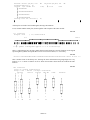
The next series shows boxplots, starting with an example illustrating the various forms boxplots can
take....
Ex.13
ÚÄÄÄÄÄÄÄÄÄÄÄÄÄÄÄÄÄÄÄÄÄÄÄÄÄÄÄÄÄÄÄÄÄÄÄÄ¿
xÄÄÄÄÄÄÄÄÄÄÄÄÄÄÄÄÄ´
*
ÃÄÄÄÄÄÄÄÄÄÄÄÄÄÄÄÄÄx
ÀÄÄÄÄÄÄÄÄÄÄÄÄÄÄÄÄÄÄÄÄÄÄÄÄÄÄÄÄÄÄÄÄÄÄÄÄÙ
ÚÄÄÄÄÄÄÄÄÄÄÄÄÄÄÄÄÄÄÄÄÄÄÄÄÄÄÄÄÄÄÄÄÄÄÄÄÄÄÄÄ¿
*
ÃÄÄÄÄx
ÀÄÄÄÄÄÄÄÄÄÄÄÄÄÄÄÄÄÄÄÄÄÄÄÄÄÄÄÄÄÄÄÄÄÄÄÄÄÄÄÄÙ
xÄÄÄÄÄÄÄÄÄÄÄÄÄÄÄÄÄÄÄÄÄÄÄÄÄÄ´
ÚÄÄÄÄÄÄÄÄÄÄÄÄÄÄÄÄÄÄÄÄÄÄÄÄ¿
*
ÃÄÄÄÄÄÄÄÄÄÄÄÄÄÄÄÄx
ÀÄÄÄÄÄÄÄÄÄÄÄÄÄÄÄÄÄÄÄÄÄÄÄÄÙ
o xÄÄÄÄÄÄÄÄÄÄÄÄÄÄÄÄÄÄÄÄÄ´
ÚÄÄÄÄÄÄÄÄÄÄÄÄÄÄÄÄÄÄÄÄÄÄ¿
*
ÃÄÄÄÄÄÄÄÄÄÄÄÄÄÄx
ÀÄÄÄÄÄÄÄÄÄÄÄÄÄÄÄÄÄÄÄÄÄÄÙ
xÄÄÄÄÄÄÄÄÄÄÄÄÄÄÄ´
@
o
o
@
o
ÚÄÄÄÄÄÄÄÄÄÄÄÄÄÄ¿
*
ÃÄÄÄÄÄÄÄÄÄÄÄÄÄx
ÀÄÄÄÄÄÄÄÄÄÄÄÄÄÄÙ
xÄÄÄÄÄÄÄÄÄÄÄÄÄ´
@ @
o
@
ÚÄÄÄÄÄÄÄÄÄÄÄÄÄÄÄÄÄÄÄÄ¿
*
ÃÄÄÄÄÄÄÄÄÄÄÄÄÄÄÄÄÄÄx
ÀÄÄÄÄÄÄÄÄÄÄÄÄÄÄÄÄÄÄÄÄÙ
ÚÄÄÄÄÄÄÄÄÄÄ¿
xÄÄÄÄ´
*
ÃÄx
o
@
@
ÀÄÄÄÄÄÄÄÄÄÄÙ
xÄÄÄÄÄÄÄÄÄÄ´
o
o
-EDA 1.4 -
@
o
@
ÚÄ¿
* ÃÄo@@@ @
ÀÄÙ 72323
@
@
@ @
@
Ex.14
Boxplot :EEE (1)
25.50
ÚÄÄÄÄÄÄÄÄÄÄÄÄÄÄÄÄÄÄÄÄÄÄÄÄÄÄÄÄ¿
xÄÄÄÄÄÄÄÄÄÄ´
*
ÃÄÄÄÄÄÄÄÄÄÄÄÄx
ÀÄÄÄÄÄÄÄÄÄÄÄÄÄÄÄÄÄÄÄÄÄÄÄÄÄÄÄÄÙ
Extreme values (LO,HI): UR
NE
Hi outliers:JU
GE
VD
NE
adjacent(LO,HI): UR
80.00
o o o
2
FR
Ex.15
Boxplot :Part90
(
4) Participation avril 1990 Tot=40.5
27.
o
ÚÄÄÄÄÄÄÄÄÄÄÄÄÄÄ¿
xÄÄÄÄÄÄÄÄÄÄÄÄÄ´
*
ÃÄÄÄÄÄÄÄÄÄÄÄÄÄx
ÀÄÄÄÄÄÄÄÄÄÄÄÄÄÄÙ
Extreme values (LO,HI): GE
Lo outliers:GE
Hi outliers:NW
ZG
SH
SH
71.
o
adjacent(LO,HI): TI
@
@
SO
Ex.16
Parallel Boxplots
23.85
69.90
ÄÄÄÄÄÄÄÄÄÄÄÄÄÄÄÄÄÄÄÄÄÄÄÄÄÄÄÄÄÄÄÄÄÄÄÄÄÄÄÄÄÄÄÄÄÄÄÄÄÄÄÄÄÄÄÄÄÄÄÄÄÄÄÄÄÄÄÄÄÄÄÄ
ÚÄÄÄÄÄÄÄÄÄÄÄ¿
RefArm :
xÄÄÄÄÄÄÄÄÄÄ´
*
ÃÄÄÄÄÄÄÄÄÄÄx o o
ÀÄÄÄÄÄÄÄÄÄÄÄÙ
ÚÄÄÄÄÄÄÄÄ¿
Roth
:
@
xÄÄÄÄÄÄÄ´
*
ÃÄÄÄÄÄÄÄx
oo
ÀÄÄÄÄÄÄÄÄÙ
2
ÚÄÄÄÄÄÄÄÄÄÄ¿
ARM
:xÄÄÄÄÄÄÄÄ´
*
ÃÄÄÄÄÄÄÄÄx
o
@
ÀÄÄÄÄÄÄÄÄÄÄÙ
Ex.17
Parallel Boxplots
0.95
69.90
ÄÄÄÄÄÄÄÄÄÄÄÄÄÄÄÄÄÄÄÄÄÄÄÄÄÄÄÄÄÄÄÄÄÄÄÄÄÄÄÄÄÄÄÄÄÄÄÄÄÄÄÄÄÄÄÄÄÄÄÄÄÄÄÄÄÄÄÄÄÄÄÄ
ÚÄÄÄÄÄÄÄ¿
RefArm :
xÄÄÄÄÄÄ´
*
ÃÄÄÄÄÄÄx o o
ÀÄÄÄÄÄÄÄÙ
ÚÄÄÄÄÄ¿
Roth
:
@
xÄÄÄÄÄ´ * ÃÄÄÄÄx
o
ÀÄÄÄÄÄÙ
3
ÚÄÄÄÄÄÄÄ¿
ARM
:
xÄÄÄÄÄ´ *
ÃÄÄÄÄx
o
@
ÀÄÄÄÄÄÄÄÙ
ÚÄÄÄÄ¿
PELec
: xÄÄÄ´*
ÃÄÄÄÄxo
ÀÄÄÄÄÙ
ÚÄÄ¿
PlArmP :´* Ã
@
ÀÄÄÙ 2
Ex.18
Boxplot :divison (
1.00
9)
4.00
ÚÄÄÄÄÄÄÄÄÄÄÄÄÄÄÄÄÄÄÄÄÄÄÄÄÄÄÄÄÄÄÄÄÄÄÄÄÄÄÄÄÄÄÄÄÄÄÄÄ¿
xÄÄÄÄÄÄÄÄÄÄÄÄÄÄÄÄÄÄÄÄÄÄÄ´
*
Ã
ÀÄÄÄÄÄÄÄÄÄÄÄÄÄÄÄÄÄÄÄÄÄÄÄÄÄÄÄÄÄÄÄÄÄÄÄÄÄÄÄÄÄÄÄÄÄÄÄÄÙ
-EDA 1.5 -
Extreme values (LO,HI): PA
Stemleaf:divison ( 9)
Legend: 1³0 stands for
1³000000000
1³
2³0000000000000000
2³
3³000000000000
3³
4³0000000000000
Density line for :divison (
²
WY
adjacent(LO,HI): PA
1.00;
4³0 for
WY
4.00
9)
Û
Û
Û
A density line is a kind of one-line histogram showing concentrations.
Let us examine another density line, shown together with a boxplot of the same variable.
Ex.19
177 countries
Boxplot :Urb
( 11) Urbanization
5.0
100.0
ÚÄÄÄÄÄÄÄÄÄÄÄÄÄÄÄÄÄÄÄÄÄÄÄÄÄÄÄÄÄÄÄÄ¿
xÄÄÄÄÄÄÄÄÄÄÄÄÄÄÄÄ´
*
ÃÄÄÄÄÄÄÄÄÄÄÄÄÄÄÄÄÄÄÄÄÄÄx
ÀÄÄÄÄÄÄÄÄÄÄÄÄÄÄÄÄÄÄÄÄÄÄÄÄÄÄÄÄÄÄÄÄÙ
²°°²±°° Û±²²²Û±±²ÛÛ±°Û°Û±Û ²ÛÛÛ±°°°²±Û±°²±±±±±°²Û°°±Û±²²±± Û±²² °± ±°± ° ±
A ‘°’ symbol corresponds approx. to 1.0 occurrence(s).
This is a coded density line: the four symbols shown code frequencies at specific locations; as the legend
says the lightest symbols corresponds here to more or less one occurrence, i.e. one country.
Ex.20
3113211 523336223442141624 34462111326213222221351125233322 52233 12 212 1 2
This is another form of the density line, showing the same information using single digits for every
location, i.e. a ‘3’ means 3 countries. A star is shown if more than 9 observations are found at the same
location.
Ex.21
183 countries
Trace of :Urb(5) Urbanization
Range: 5.00 - 100.00 ; Groups: Continents
g# Asia
Africa
Europe
N&C.Am
S.Am.
x :
x
x
x
³ : ³
³
³
³ : ³
³
³
x
³ : ³
ÚÁ¿
³
ÚÁ¿
³ : ÚÁ¿
@
³ ³
ÚÁ¿
³ ³
ÚÁ¿ : ³ ³
o
³*³
³ ³
³*³
³ ³ : ³ ³
x
³ ³
³ ³
³ ³
³ ³ : ³ ³
³
ÀÂÙ
³*³
³ ³
³*³ : ³*³
³
³
³ ³
³ ³
³ ³ : ³ ³
³
³
ÀÂÙ
ÀÂÙ
³ ³ : ³ ³
ÚÁ¿
³
³
³
³ ³ : ³ ³
³ ³
x
³
x
ÀÂÙ : ³ ³
³*³
o
³
³ : ÀÂÙ
ÀÂÙ
x
³ : ³
³
³ : ³
³
o
x :
x
x
N
39
53
30
31
15
-EDA 1.6 -
AusOcea
x
³
³
³
ÚÁ¿
³ ³
³ ³
³ ³
³*³
³ ³
ÀÂÙ
³
x
15
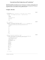
EDA Software: First steps
Before starting to work with the EDA package you need to know how to call EDA on your computer and
how to write EDA commands.
How to write EDA commands
You interact with EDA using simple commands. There is no difference between commands written in
lower or upper case letters.4 In the various examples and in the manual however we will always use
upper case letters for commands and options. Lower case letters will be used for parts of commands you
should supply (variable names etc.)
For clarity all command line examples will be preceded by the > symbol. This symbol is not part of the
command and should never be typed.
For instance
>GET name
GET is the name of the command to be typed (in upper or lower case letters). name: you should supply a
valid name (name of a work area = data set).
>GET SET2
is an command as you might type it, i.e. SET2 is a work area name. (Uppercase because this is an acutal
command line example).
>BOXPLOT 1
>BOXPLOT 1,2,4
>BOXPLOT 1-10 PARALLEL
>BOXP 1-10 PAR
The four examples produce boxplots. The first example displays a boxplot for variable number 1; the
second three boxplots for variables 1,2 and 4. Thee third example produces parallel boxplots for all
variables from 1 to 10; PARALLEL is an option. The last example is identical to the third, except that it
shows that you need not type all letters. 1; 1,2,4 and 1-10 show various forms of variable lists. Variable
lists are always specified immediately after the command name (before any option).
Data in EDA
Data you want to analyse has to be brought into the EDA work area, i.e. the active data matrix (data
sheet). The GET command reads a data-set5 into the EDA Work Area (WA), i.e. the data matrix to be
analysed.
Use the DIR6 command to see a list of available datasets. This command will show the name and a short
description of all datasets in the EDA library, i.e. the data sets available with a GET command.
Syntax conventions
The user’s manual and the on-line help use a number of syntactical conventions. If you type:
>?STEMLEAF
you will see the syntax of the STEMLEAF command: Do not worry if you do not understand all the
details of the command itself, concentrate on the syntactical constructs used.
_______________________________________________________________________________________________________________________
4. Later we will learn that case and variable names are case-sensitive.
5. The data sets read by GET are EDA specific system files, i.e. the only software package that can read and produce them is EDA. Of course EDA
has a number of commands to bring in data from the “outside world”, namely the *READ command and its many options. But start to learn how
to work with EDA using the various data sets which are readily available.
6. Note that this is an EDA command, and NOT the DOS DIR command.
-EDA 1.7 -
STEMLEAF
STEMLEAF
STEMLAEF
STEMLEAF
v <opt>
v BYGVAR{=gvar#} [NGROUPS=ng] <opt>
v SPLIT (log-expression) [PARALLEL] <opt>
v1,v2 <opt>
<opt> [SCALE=value] [WIDTH=chars]
[NOLINE] [NOHILOSTEM]
[ASCENDING|DESCENDING]
There are four different forms (producing variations of the stem and leaf-plot) of the command each of
them sharing a number of common options. A number of metasymbols7 are used:
v
[]
{}
|
<opt>
Refers to a single variable
Used to indicate an option
Options within options
Select one (alternatives). In the [ASC|DESCENDING] example
select either ASC or DESC, if you use this option ([]= option)
see definition of <opt> elsewhere, usually below
Even though syntax diagrams might look complex, sometimes frightening, make sure to understand that,
the actual command you are typing will often be very simple, e.g. STEMLEAF 1, sometimes with an
option or two.
A first list of commands
These commands perform common tasks and are useful to learn about exploratory tools. All of them are
straightforward to use and to understand (from the output they produce). You are invited to try them out.
GET
DIR
name
DESCRIBE
DESCRIBE
Gets a work area from the archive library
Shows the work areas in the archive library
vlist
ALL
display variable info. (labels and descriptors)
display variable info for all variables in the WA
STEMLEAF
produces a stem and leaf plot
HISTOGRAM
shows a histogram
HISTOGRAM vlist BAR “classical” histogram
LIST
listing variables, many options (coded etc)
SHOW
conditional lists SHOW FAR shows only outliers
BOXPLOT
displays a box-and-whisker plot
PARALLEL
parallel boxplot
SUMMARY
numerical summaries (5-number summaries etc)
DISPLAY
numerical summaries (MEDIAN MEAN etc)
QSUMMARY
quick summaries
DLINE
density lines (single line histograms)
CODED
coded density lines
PLOT
plot two or more variables (many forms)
PI
plot inspect module
Controlling screen output
Most commands produce output in a way that you can see all information on a single screen. There are
however exceptions: output from commands producing lists usually does not fit on a single screen.
Commands like the LIST or DIR command will, by default, automatically page the output, i.e. after a
screenfull of output, the display stops and you are invited to hit the return key to see the next screenfull8
The are some situations however where the information quickly scrolls off the screen and when the
screen stops you are looking at the bottom of the display. In this situation you might use the <PAUSE> or
<SCROLL-LOCK> keys on your PC to stop scrolling or you might tell EDA to stop after each screenfull
of information: this is done with the SET PAGE ON command (turns paging on; SET PAGE OFF turns it
off).
_______________________________________________________________________________________________________________________
7. Metasymbols are symbols used to explain the syntax and are not used in actual commands
8. You are also offered the choice to stop at that point.
-EDA 1.8 -
Additional information
Type INFO INFO to see what other course specific on-line information is available.
Basic information (command lists, general concepts etc) can be obtained from the HELP command;
syntactical information on a specific command is produced by ?<name>, where name is the name of a
valid EDA command.
-EDA 1.9 -