1
Chapter 1 – An Overview of MIDUSS 98
Chapter 1 - An Overview of MIDUSS 98
The following general areas describe the overall purpose of the MIDUSS 98 program, the structure of the
main menu, major differences from previous versions of the program and a description of the functionality
available in MIDUSS 98.
•
Chapter 1 - Overview of MIDUSS 98
•
Chapter 2 - Structure and Scope of the Main Menu
•
Chapter 3 - Hydrology Used in MIDUSS 98
•
Chapter 4 - Design Options Available in MIDUSS 98
•
Chapter 5 - Hydrograph Manipulation.
•
Chapter 6 - Working with Files
•
Chapter 7 – Hydrological Theory
•
Chapter 8 - Theory of Hydraulic Design.
•
Chapter 9 - Displaying Results.
•
Chapter 10 - Running in Automatic Mode
•
Chapter 11 - A Detailed Example
•
Appendix ‘A’ - References
•
Appendix ‘B’ – Transferring a Licence
Refer to the relevant chapter for more information
This help document created 1998-08-24
An Introduction to MIDUSS 98
The MIDUSS 98 package was developed to help drainage engineers to design the hydraulic elements in
a collection network of storm sewers or channels. The program does not make design decisions but
rather carries out hydrological and hydraulic analyses and presents you with design alternatives. It is
then left to you as the engineer to select values for the design variables and to decide on the acceptability
of a design.
MIDUSS 98 is highly interactive in use, and allows engineering judgment to be exercised at all stages of
the design process. Moreover, this interaction lets you monitor each step of the process and take
corrective action in the event of an error. With most commands, data is input in response to prompts,
and you are free from the need to prepare lengthy data files prior to the design session. In many cases a
design session will require to be repeated either:
1.
to test a previously designed system under a different storm,
2.
to continue or modify a previous design session.
3.
to modify a hydrology or design parameter.
1
2
Chapter 1 – An Overview of MIDUSS 98
Using Automatic Mode
When a design session has to be repeated with a modification such as a different storm, it is possible to
use an input file which contains a log of the previous session with all the commands and the relevant
data. In MIDUSS 98 this input file is in the form of a database which can be produced automatically from
a previously created output file. Running MIDUSS 98 in automatic mode eliminates the need to re-enter
the commands and data from the keyboard. In this mode, however, design decisions with respect to
pipes, ponds, channels or diversion structures can still be altered and changes can be made to the
database. The use of files in this way is discussed in more detail later in this Help file. (see Chapter 10 Running in Automatic Mode)
The hydrology and hydraulics used in MIDUSS 98 is based on well established and accepted principles.
The details of these techniques are described under the various command headings in Chapter 3 Hydrology Used in MIDUSS 98 and Chapter 4 - Design
Sections have been added which presents the relevant background theory. These need not be studied in
order to run MIDUSS 98 but have been included for the interested reader or student.
The next section provides a general description of a typical design session A more detailed example is
presented in Chapter 11 – A Detailed Example .
A Simple Example
A Typical Design Session
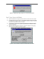
Assuming you have pressed the [Yes] button when the initial Disclaimer form is displayed, MIDUSS 98
starts up with the main menu displayed at the top of the window. Depending on the size and resolution of
your screen you will probably want to click on the ‘maximize window’ symbol at the right hand end of the
title bar to make the MIDUSS 98 window fill the screen.
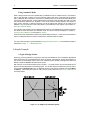
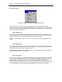
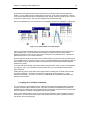
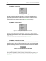
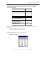
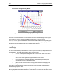
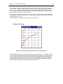
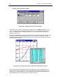
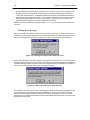
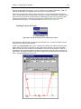
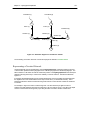
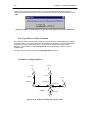
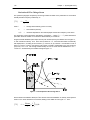
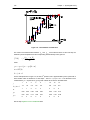
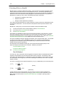
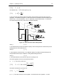
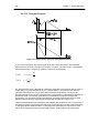
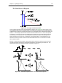
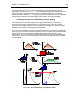
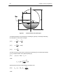
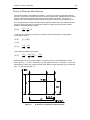
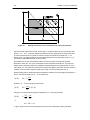
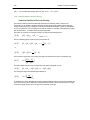
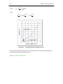
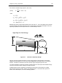
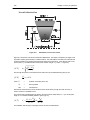
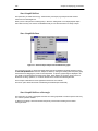
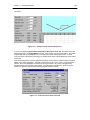
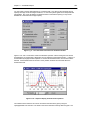
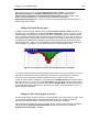
With reference to the simple example shown in Figure 1-1, a typical session may be summarized by the
sequence of steps described in the following topics. You are first required to define the system of units to
be used and the Options/Units menu is displayed with the mouse pointer positioned over either Metric
or Imperial. After setting the system of units, your first action should be to define the Output File to
record the session.
Figure 1-1 – A Simple Two-catchment System
Chapter 1 – An Overview of MIDUSS 98
Define the Output File
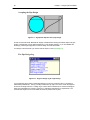
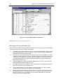
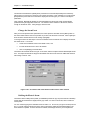
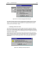
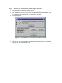
Using the File/Output/Create New File menu item, navigate through the standard Windows95 Common
Dialog Box to select an existing file or create a new one in a directory of your choice. This directory will
serve as the Job Directory for this session and the file will contain a record of the commands used, the
data entered and some of the results. The Job Directory will also contain any files which you create such
as storm or hydrograph files.
If you omit this step MIDUSS 98 will use a default output file (called ‘default.out’ ) which resides in the
Miduss98 directory e.g. C:\Program Files\Miduss98\. Using this file is not recommended since it results
in an accumulation of files in the Miduss directory. Also, the default output file may be overwritten during
the next design session if you again use the default condition.
After setting the Job Directory the next logical step is to Select your Options
Select your Options
MIDUSS 98 offers a number of features most of which are optional. The most important is the system of
units to be employed. Immediately following acceptance of the Disclaimer form you will be prompted to
select the system of units to be used for the session. Your choice for units and other options will be
remembered when the session is finished and MIDUSS 98 will start the next session with the same
selection.
Other options let you show or hide the status bar, use the MIDUSS 98 tool tips, or enable a system of
prompts which you may find useful as a first time user of MIDUSS 98.
Before you can proceed to any hydrological modelling you must set the Time parameters and this
should be your next step.
Set the Time Parameters
In the Hydrology menu all of the options are initially disabled with the exception of the Time
parameters. This command prompts you to set the time step, maximum storm duration and longest
hydrograph duration you expect to use. All of these values are defined in minutes. Be generous with the
estimate of storm duration and hydrograph length because if you find you want to define a storm longer
than you originally thought a second use of the Hydrology/Time parameters command will cause the
arrays storing rainfall and hydrographs to be re-initialized with loss of data.
Setting the time parameters will also enable the Storm command and your next logical step will be to
Define the Design Storm .
Define the Design Storm
Use the Hydrology/Storms command to define a single event design storm using one of five methods
i.e.
•
a Chicago storm,
•
one of the four Huff distributions,
•
any of the pre-defined mass rainfall distribution (*.mrd) patterns,
•
a storm pattern as proposed by the Canadian Atmospheric Environment Service (AES), or
•
a historic storm
Alternatively, you could import a previously created storm hyetograph file by means of the File I/O
command.
Either method causes the Hydrology /Catchments command to be enabled. The rainfall defined in this
way remains in force until the rainfall is redefined. Normally the storm is defined only once at the start of
the session.
Once the storm is defined the next step is to generate the Runoff Hydrograph for the first catchment area.
3
4
Chapter 1 – An Overview of MIDUSS 98
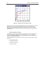
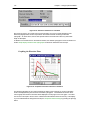
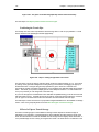
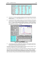
Generate the Runoff Hydrograph
Using the Hydrology/Catchments command you can now define the first catchment and produce the
direct runoff hydrograph for the previously defined storm event. The runoff hydrograph is stored in the
Runoff hydrograph array.
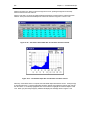
The runoff is computed separately for the pervious and impervious fractions of the catchment and the two
hydrographs are added. Information about the catchment runoff is provided in various ways;
•
A table is displayed with the flow for each time step together with the peak flow and the total
volume of runoff.
•
A graphical display shows the runoff from the pervious and impervious fractions as well as the
total runoff.
•
A table of rainfall and runoff measures can be displayed by clicking on the [Show Details] button.
•
Another summary table shows the history of peak flows in each of the four arrays for Runoff,
Inflow, Outflow and Junction hydrographs, but this is not updated until you have accepted the
results of the calculation by pressing the [Accept] key.
Accepting the computed runoff hydrograph causes the menu command Hydrograph /Add Runoff to be
enabled. Using this the Runoff is added to the current Inflow hydrograph which in this case is initially
zero. The summary table of hydrographs is updated.
Before you can use this hydrograph to design an element of the drainage network you must add the
runoff to the current Inflow hydrograph. This is done by using the Hydrograph/Add Runoff command .
Using the Add Runoff Command
The Hydrograph menu contains a number of options to manipulate flow hydrographs. These are initially
disabled and become available to you as the pre-requisite steps are completed. Once a new runoff
hydrograph has been created by means of the Hydrology/Catchments command the Hydrograph/Add
Runoff command is enabled.
This command causes the last computed runoff hydrograph to be added to the current Inflow hydrograph.
The result of this operation is shown in the summary of peak flows. The Hydrograph/Undo command is
enabled by this action so that you can reverse the process should you wish to do so.
Now that the Inflow hydrograph has been updated the next logical step is to design an element of the
drainage network such as a pipe or channel or other facility. Open the Design menu and select an item
to design a pipe or channel .
Design a Pipe or Channel
Using one of the options in the Design menu, you can now design a pipe or channel to carry the peak
flow of the Inflow hydrograph. For each of the Design menu items default data is displayed which you
should change to suit your requirements. Your data values will become the new default values for the
remainder of this session or until changed again.
Design of pipes or channels requires selection of a depth or diameter along with the gradient expressed
as a percentage. Pressing the [Design] command button causes a uniform flow analysis to be displayed
which shows the actual depth, the flow capacity of the conduit, the average velocity and the critical depth
of flow to indicate whether the flow will be sub-critical or super-critical.
In the case of a pipe the design may result in surcharged conditions in which case the hydraulic grade
(i.e. the slope of the energy line) is reported. Surcharged flow may result in only a portion of the runoff
being captured so that the total runoff must be split between major (i.e. on the surface or street) and
minor flows (i.e. in the pipe).
Of course, options other than the Pipe and Channel design may be used but these simple cases are used
for this introductory description,
When the design is accepted the Design/Route menu item is enabled which lets you route the flow
hydrograph through a specified length of conduit.
Chapter 1 – An Overview of MIDUSS 98
Route the Hydrograph
The Design/Route menu command is used to route the hydrograph through a user-defined length of the
most recently designed conduit. After accepting the result, the peak of the outflow hydrograph is
displayed in the summary table of hydrograph peaks.
When an outflow hydrograph has been created by some routing operation you may choose from two
possible courses of action. Either the outflow can be copied to the inflow array in order to continue to the
next downstream link, or the outflow may be stored at a junction node to be combined with other flows at
a confluence point.
For this example you should assume that the outflow from the first conduit will form all or part of the
inflow to the next downstream conduit. You can do this by using the Hydrograph/Next Link menu
command in the Hydrograph menu.
Using the Next Link command
When a new outflow hydrograph is created, the Hydrograph/Next Link menu item is enabled. Using this
command causes the outflow hydrograph to be copied to replace the inflow hydrograph and ready to
receive the runoff contribution from the next sub-catchment. If no additional catchment runoff enters at
this point you can simply use the inflow to design another link in the drainage network such as a
detention pond, an exfiltration trench or a diversion structure.
For this example a second catchment area must be defined and the runoff added to the total inflow. The
procedure for modelling the second catchment is similar to the previous case. If the parameters
describing the rainfall losses and infiltration are unchanged, the effective rainfall for the pervious and
impervious areas will also be unchanged and only the calculation of runoff is required. One exception to
this rule is when using the SWMM Runoff procedure to model the overland flow. Refer to Chapter 7
Hydrological Theory – The SWMM Runoff Algorithm for more information.
Once the runoff from the second catchment has been accepted you can use the Add Runoff command a
second time to accumulate the flow in the inflow hydrograph.
Add Runoff Hydrograph #2
The Hydrology /Catchments is used a second time to generate the runoff hydrograph from the next
catchment area. The Hydrograph /Add Runoff command causes this to be added to the Inflow
hydrograph. Both changes are reflected in the summary table of peak flows.
For this simple example the next and final step is to design a detention pond to reduce the peak flow.
Design a Detention Pond
To reduce the peak of the Inflow hydrograph, the Design/Pond menu command is used to design a
detention pond. The process requires the calculation of the Stage - Discharge - Storage Volume data for
the pond. A number of options are available in the Design/Pond command to let you describe different
parts of the outflow control device. These may comprise multiple orifices and weirs from which the Stage
- Discharge curve is computed. Options are also available to help you calculate the Stage - Volume
Storage curve for a few standard forms of storage geometry such as an idealized pond of rectangular
shape, large diameter "super-pipes", wedge storage on graded parking areas or rooftop storage.
When you use the Design/Pond command you can specify the desired peak outflow and MIDUSS 98 will
suggest values of storage and other parameters which will provide an initial design. You can then fine
tune the design until you are satisfied with the result. Since this is a trial and error procedure the Design
Log feature of the Design options is useful in summarizing the progress of this iterative procedure.
The Outflow hydrograph is obtained by a storage routing procedure and the attenuated peak flow is
displayed in the table of peak flows. MIDUSS 98 will automatically adjust the storage routing time-step to
ensure numerical stability in the vicinity of highly nonlinear Discharge - Storage Volume curves. Any
such adjustment is reported but otherwise the process is transparent to the user.
This concludes this simple illustrative example but you may find it useful to review the summary of
modelling procedure which follows. A more detailed example is presented in Chapter 11 – A Detailed
5
6
Chapter 1 – An Overview of MIDUSS 98
Example.
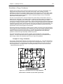
Summary of Modelling Procedure
(1)
The total catchment area is subdivided into a series of sub- catchments, each of which generates
an overland flow or runoff hydrograph. The hydrograph is assumed to enter the drainage network
at a particular point or node associated with the sub-catchment. The drainage network is
assumed to be a tree so that each node can have any number of inflow links but only one outflow
link. For this reason, each link is given the same number as the node at its upstream end. These
sub-catchments are processed in order, starting at the upstream limit of sewer branches and
working in the downstream direction.
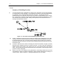
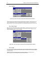
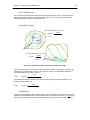
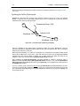
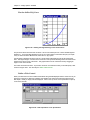
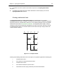
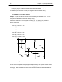
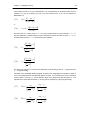
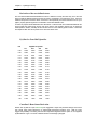
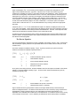
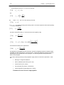
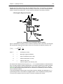
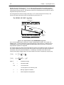
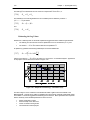
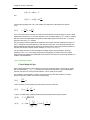
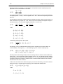
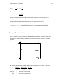
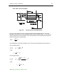
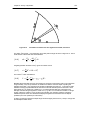
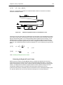
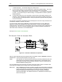
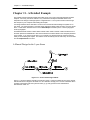
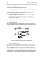
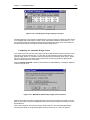
Figure 1-2 – Convention used for Numbering Nodes and Links
(2)
Figure 1-2 illustrates a node (102) which receives the outflow from the upstream link (101), adds
to this the runoff from catchment (102) and creates the resulting inflow hydrograph to be carried
by the downstream link (102). The node number is defined as the ID number of the catchment
and sets the reference number for the element of the drainage network from this point to the next
downstream node.
(3)
The links or branches of the network connecting the nodes are assumed to be pipes, channels,
detention ponds, exfiltration trenches or diversion structures. As each runoff flow hydrograph is
added to the flow in the system, a pipe, channel, pond, etc. can be proportioned to carry the peak
inflow. Once this element has been designed the inflow hydrograph is routed through the link to
produce an outflow hydrograph.
(4)
Steps (1), (2) and (3) are repeated, moving downstream, accumulating overland flow from each
sub-catchment or storing an outflow hydrograph in order to design another branch meeting at a
confluence point. Refer to Chapter 5 – Hydrograph Manipulation for more details.
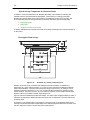
Chapter 2 – Structure and Scope of the Main Menu
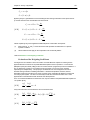
Chapter 2 - Structure and Scope of the Main Menu
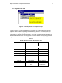
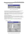
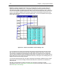
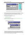
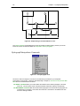
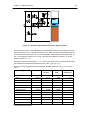
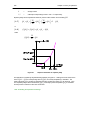
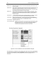
Figure 2-1 – The Main Menu with all items enabled
When you first start MIDUSS 98 a number of the items in the Main Menu will be grayed out or disabled.
This indicates that some prerequisite information has not yet been defined. For example, the Storm
command is not enabled until you have defined the time step and storm and hydrograph duration to be
used. Similarly, the Catchment command cannot be used until a storm has been described. In the
Design options, components such as a detention pond or ex-filtration trench require an Inflow hydrograph
to have been created.
You will notice an apparent contradiction to this general rule. In the Pipe and Channel commands, it is
possible to use these without having previously computed the inflow hydrograph. If no inflow hydrograph
exists you can still use the Pipe or Channel command but you will have to enter a value for the peak flow
instead of having that supplied as the peak flow of the inflow hydrograph. This allows you to use the Pipe
and Channel commands for design purposes without having to go through any hydrological modelling.
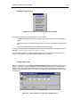
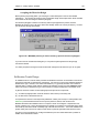
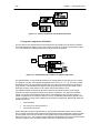
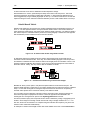
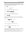
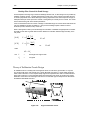
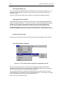
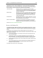
The File Menu
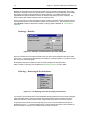
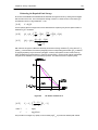
Figure 2-2 – The File Menu Options
The File Menu includes items to:(1) Create an Input Database (using a previously created Output file) for use in Automatic mode.
(2) Open an Output file - either creating a new file or overwriting an old one.
(3) Set printer parameters
(4) Set scaling factors and print hardcopy from the MIDUSS 98 window or the whole screen
(5) Abandon results generated up to this point and start over.
(6) Exit from MIDUSS 98
7
8
Chapter 2 – Structure and Scope of the Main menu
Refer to The Automatic Mode later in this chapter or Chapter 10 Running MIDUSS 98 in Automatic Mode
for information on creating and using the Input database Miduss.Mdb.
Open Input File
When you run MIDUSS 98 in Automatic mode the input is read from a data base file called Miduss.Mdb.
This file is created from an Output file which has been generated during a previous run of MIDUSS 98 usually in manual mode, or in automatic mode with significant editing changes of the input data. Only
one copy of Miduss.Mdb can exist in the MIDUSS 98 directory. However, you can save a copy under in a
different directory
The Open Input File command allows you to open a previously created output file and convert it to a
database with the name Miduss.Mdb. If a previously saved file of this name exists you will be warned
that this will be overwritten.
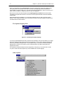
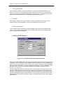
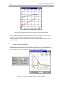
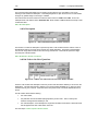
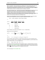
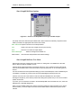
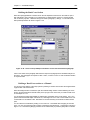
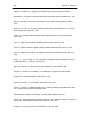
Output File command
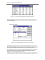
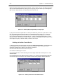
Figure 2-3 – Using the File Menu to define an Output File
During a MIDUSS 98 run the commands used, the data entered and some of the results are always
copied to an output file. If you do not specify an output file in a particular Job Directory the output goes to
a file called Default.Out which is created in the MIDUSS 98 directory. This menu item allows you to
specify an alternative to the default file.
You can choose between creating a new file or selecting an existing file. If you use the name of an
existing file you will be warned that the file will be overwritten and the contents will be lost.
In both cases you select the directory and enter or select a file name by means of the standard File Open
dialogue box. You can use long file names to relate the file to the design situation e.g. "PineView_5yr_post-dev.out"
Print Setup
This command opens up the standard Windows dialog box to set up certain parameters for your printer.
When you press [OK] a message box is displayed giving you the option to print either the full screen or
the MIDUSS 98 window. See the Print Command for further details.
Chapter 2 – Structure and Scope of the Main Menu
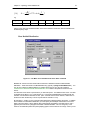
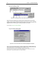
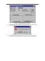
Print command
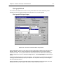
Figure 2-4 – Options available using the File/Print command
As illustrated in Figure 2-4, the print command contains a number of sub-commands which let you:
(1) Set the scale of the hardcopy relative to the page size
(2) Print the entire screen
(3) Print only the MIDUSS 98 window
(4) Clear the buffer containing data to be printed
When you select the Scale command you can choose from a number of standard ratios such as 100%,
75%, 50% & 25%. If none of these is suitable you can specify another ratio which will be saved for future
use during the current session. After a scale has been selected the Print menu item is modified to show
the currently selected scale.
Quit and Start Over
You may want to use this command if you realize that the work done so far is of no value and you want to
abandon the session but immediately restart MIDUSS 98. It is equivalent to the Exit command followed
by an immediate re-run of MIDUSS 98. See File/Exit command for more details.
File Exit
This command ends the MIDUSS 98 session. Files created during the session will be closed and the
current Options in effect will be saved for use as the initial defaults in the next session.
Two files may be worth saving before your next run of MIDUSS 98.
(a)
If you did not specify a Job directory, the output will be stored in the default output file
C:\Program Files\Miduss98\default.out. If you want to keep this you must rename it or copy it to
another file or another directory. The default output file will be overwritten at the start of the next
MIDUSS 98 session which does not use a specified Job directory.
(b)
The file C:\Program Files\Miduss98\Design.log will contain a record of any design commands
which you used. This may be of use in interpreting the output file or for making comparisons
during your next MIDUSS 98 session.
9
10
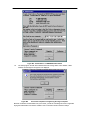
Chapter 2 – Structure and Scope of the Main menu
Figure 2-5 – Warning displayed if an Error Log is created.
Sometimes if an error occurs during the MIDUSS 98 session you will see a message that a file
Miduss.Log has been created. This will contain information of errors that were trapped by MIDUSS 98. It
would be useful if you could forward this file to Alan A. Smith Inc. either by e-mail or by Fax so that the
cause of the problem can be corrected.
The Options menu item
Figure 2-6 – The three main choices in the Options Menu
The fragment of menu illustrated in Figure 2-6 shows the three sub-menu choices available. These allow
you to
•
Select the system of units to be used,
•
Select English or an optional second language for the display of screen text and
•
Select and set a number of other options and preferences.
The Second Language option is enabled only in copies of MIDUSS 98 which have been customized for
a language other than English.
Note: If you exit normally from MIDUSS 98 the preferences in effect will be recalled the next time you
run MIDUSS 98. Click on the menu item or the highlighted text for further details.
Chapter 2 – Structure and Scope of the Main Menu
11
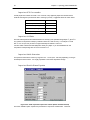
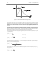
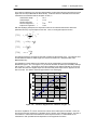
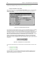
The Options Units item
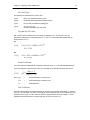
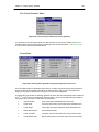
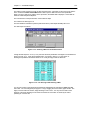
Figure 2-7 – Selecting the units is a required first step.
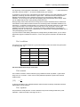
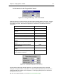
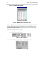
As shown in Figure 2-7, you can select between two systems of units. In the metric system the unit of
length is the metre or millimetre depending on the variable being defined. In the Imperial system (also
known as U.S. Customary units) length is defined in feet or inches.
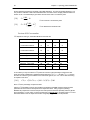
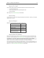
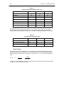
In MIDUSS 98, only kinematic units are employed, i.e. only length, area, volume and time dimensions are
used. The Table below shows the units employed for the various quantities used in hydrology and in the
design of storm water management facilities.
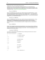
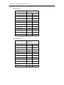
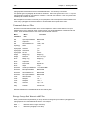
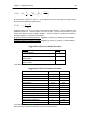
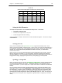
Table 2.1
Variable dimensions used for SI and Imperial units
QUANTITY
Time
Imperial
Metric
(US Customary)
(SI units)
seconds, minutes or hours
Rainfall depth
inches
millimetres
Rain intensity
inches/hour
millimetres/hour
Catchment
acres
hectares
Length
feet
metres
Diameter
feet
metres
Surface area
square feet
square metres
Velocity
feet/second
metres/second
Flow rate
cubic feet/sec
cubic metres/sec
Volume
cubic feet
cubic metres
acre-ft
hectare-metre
12
Chapter 2 – Structure and Scope of the Main menu
When you start MIDUSS 98 the Options/Units menu item is automatically selected and displayed with
the mouse pointer on the system of units which is stored in the Registry and which is therefore the
current default. As shown in Figure 2-7, most of the menu items are disabled in order to force the user to
either confirm the default or change the system of units to be displayed.
Both choices of units will remain enabled until the Hydrology/Time parameters menu item has been
completed and accepted after which the menu items for both Imperial and Metric units will be disabled
but still visible.
When MIDUSS 98 is first installed on your computer the default system of units is the metric system.
However, if you change the selection your choice will be recorded in the system registry and will form the
new default value for future sessions.
The Options Language item
Figure 2-8 – Selecting the Display language
If you have purchased MIDUSS 98 with an optional second language, this menu item allows you to toggle
the screen displays between English and the second language. You can switch between languages at
almost any point during a design session. One exception is when a warning or information message is
displayed which requires you to press one of the command buttons (e.g. [OK] or [Yes]) before the
program will continue.
The translations will almost always have been prepared by a third-party (i.e. other than Alan A. Smith
Inc.) and in certain cases this Help file may not be available in the second language.
Other Options
Chapter 2 – Structure and Scope of the Main Menu
13
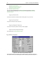
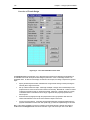
Figure 2-9 – Other options available in MIDUSS 98
As illustrated in Figure 2-9, the available options with the current release of MIDUSS 98 are as follows.
Show Text Box Tips. Selection of this option triggers a display of a brief explanation of the data item
when the mouse pointer is over a text box; sometimes a range of typical values is displayed. The tip can
be displayed in a small yellow window adjacent to the text box or in the status bar by selecting one or
other of the two options shown below.
On Form
On Status Bar
Set Delay for Text Box Tips
Specify the delay in milliseconds before the tip is shown.
These menu choices are disabled (grayed out) if Show Text Box Tips is not selected. If Show Text
Box Tips is selected, the active menu item is shown with a check-mark. You can also toggle between
showing or not showing the Text Box Tips by pressing Ctrl-T. (i.e. Hold down the Control key and press
'T')
You will probably find the Text Box Tips option useful during your first few sessions with MIDUSS 98.
When you are familiar with the data requirements it can be turned off.
Highlight Text boxes. When this option is selected it causes the current contents of a text box to be
highlighted when the text box receives the focus. You may find this preferable since it allows you to start
typing a value from the left character position instead of having to use the backspace key or an arrow key
to position the text entry marker at which keystrokes will be entered. Note that this option does not apply
to data entry in a grid.
Show Status bar. When this menu item is checked the status bar is enabled at the bottom of the
MIDUSS 98 window. The status bar contains information about the current menu selection, the job
directory and output file and whether MIDUSS 98 is in Automatic or Manual mode.
Show Prompt messages after each step. This causes a brief message to be displayed after many
commands to advise you on the action taken and suggest one or two logical next steps. When used
together with the Show Next logical menu item option these options provide useful guidance if you are
unfamiliar with the MIDUSS 98 program.
Show Next logical menu item. After completion of a command, and after display of the Show Prompt
messages after each step message if selected, this option causes the next logical menu item to be
displayed with the mouse pointer positioned over the appropriate command as a guide to the user.
Maximum number of decimal places. In some displays of data or results you may require to increase
the number of figures after the decimal point to get sufficient accuracy. Selecting this command opens a
simple data entry window with a prompt to enter a single digit specifying the maximum number of places.
Highlight Maximum Value. In many commands a rainfall hyetograph or flow hydrograph is displayed in
tabular form. Selecting this option causes the cell containing the maximum value to be coloured light
cyan.
14
Chapter 2 – Structure and Scope of the Main menu
The Hydrology Menu
Figure 2-10 – Commands for Hydrologic simulation.
The Hydrology menu allows you to set the Time parameters and use the Storms and Catchments
commands to generate the direct runoff hydrograph. Other options include a Lag and Route procedure to
allow very large sub-catchments to be modelled with realistic overland flow lengths. An option is also
included to let you specify Base Flow.
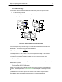
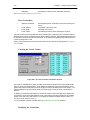
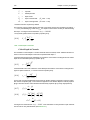
Hydrology Time Parameters
Figure 2-11 – The default time parameters
When you start MIDUSS 98 this is the only item in the Hydrology Menu which is enabled. None of the
other options can be used until you have specified the three time parameters shown here. Many of the
items in the MIDUSS 98 main menu are also disabled until the time parameters have been specified.
The specification of the time parameters should be preceded only by the specification of the system of
units to be used and(if desired) the specification of a job-specific directory and output file.
The three time parameters are:
Time step:-
The time interval in minutes to be used for all rainfall runoff calculations
and routing operations in pipes, channels, ponds or trenches. A value
of 5 minutes is common but a smaller time step is seldom justified.
Longer increments of 10 or 15 minutes may be used for long storms.
Note that for some routing operations a sub-multiple of the time step is
used to ensure numerical stability. If you intend to use the Chicago
storm with a very small time step consider using the time step multiplier
to avoid very large values of peak rainfall intensity.
Maximum storm duration:-
The longest storm duration which you expect to use during the current
session. This sets the length of array used for hyetograph storage. A
value of 3 to 6 hours (180 to 360 minutes) is common.
Chapter 2 – Structure and Scope of the Main Menu
15
Maximum hydrograph length:- The longest expected hydrograph duration for the current session.
This sets the length of storage array used for hydrographs. A 24-hour
hydrograph (1440 minutes) is not unreasonable.
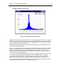
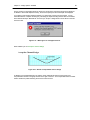
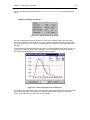
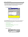
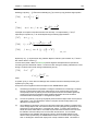
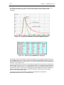
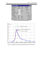
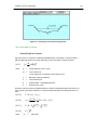
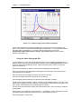
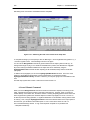
Hydrology Storm
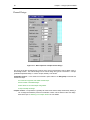
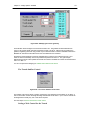
Figure 2-12 – The five options available in the Storm command.
Use this menu option to specify a single event storm hyetograph. Typically this is done only once at the
start of the session and applies to all of the catchment areas; however, there may be circumstances
when a different storm may be required for a portion of the total area being modelled - e.g. higher
elevation or a lagged, travelling storm.
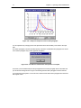
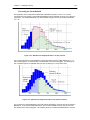
The five tabs on the form provide five options to define four different types of design storm or a historic
storm. In every case you are prompted to supply parameter values or use the default values displayed.
Pressing the [Display] button causes a table of rainfall intensities and a graphical plot of the hyetograph
to be displayed.
You can experiment by changing parameter values or even storm type and update the displays by
pressing [Display]. When you are satisfied with the storm press the [Accept] button to cause the storm to
be defined. This remains in effect until it is changed by a subsequent use of the command.
Note that you can use the File Input/Output command to import a hyetograph file as an alternative to
using the Storm command. Such files can be saved by means of the same File Input/Output command
after a storm hyetograph has been defined – especially a long historic storm.
After you have accepted the design storm, an auxiliary window is opened prompting you to enter a string
of up to 5 characters which is used as a descriptor of the storm just defined. This descriptor is used as
part of the filename of any hydrographs stored as files during the current session. Refer to the
Hydrology/Storm Descriptor command for more details.
See Chapter 3 Hydrology Used in MIDUSS 98 Storm Command for more details.
16
Chapter 2 – Structure and Scope of the Main menu
Hydrology - Storm Descriptor
Figure 2-13 – Defining a Storm descriptor
The window shown in Figure 2-13 is opened automatically after you have pressed the [Accept] button in
the Storm command form. The string requested will be used as part of the name given to any
hydrograph files which are generated in the current session using this design storm.
Typically you may enter the return period for the storm - e.g. "005" to denote a storm with a return interval
of 5- years. When you save a hydrograph as a file the default extension used by MIDUSS 98 is ".hyd".
The filename which you provide has the Storm Descriptor added to this extension to give a modified
extension of ".005hyd".
For example, if you specified a filename of "Pond7aOut" and the Storm Descriptor is "005" the final
filename would be "Pond7aOut.005hyd".
Windows 95 allows long filenames and also allows more than one 'period' separator. You can define the
Storm Descriptor with a period at the end (e.g. "005."). Using the previous example, the resulting
filename will be "Pond7aOut.005.hyd". However, you may find that this results in confusing abbreviations
if the filename is displayed in a DOS window.
As a reminder of the descriptor that you have entered it is appended to the Storms item in the
Hydrology menu. Refer to the Hydrology menu earlier in this chapter to see this (Figure 2-10).
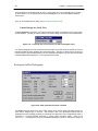
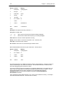
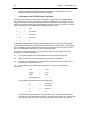
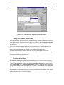
Hydrology Catchment
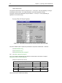
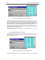
Figure 2-14 – Data input form for the Catchment command
Chapter 2 – Structure and Scope of the Main Menu
17
Once a design storm has been defined, you can use the Catchment command to generate the direct
runoff hydrograph for a sub-catchment. The three tabs on the form are used as follows.
Catchment
Set the methods and parameters for the whole catchment and generate the overland
flow hydrograph on the pervious, impervious and total areas.
Pervious
Set the rainfall loss model and the appropriate parameters to generate the effective
rainfall on the pervious fraction of the area.
Impervious
Set the parameters for the impervious fraction and generate the effective rainfall on the
impervious fraction of the area.
The command contains a number of options for the overland routing method, the relative flow length on
the pervious and impervious fractions of the catchment and the method to be used to estimate rainfall
losses by infiltration, interception or surface depression storage.
Before calculating the runoff it is necessary to compute the effective rainfall on both the impervious and
pervious surfaces. This can be done explicitly by selecting the appropriate part of the form or it can be
done automatically if you select the runoff calculation option.
Special conditions apply if you select the SWMM Runoff algorithm as the overland routing method since it
uses a surface water budget method rather than an effective rainfall approach.
The command is described in full in the Hydrology section of this Help System. Refer to Chapter 3
Hydrology Used in MIDUSS 98, Catchment Command for more details.
Note that you can use the File Input/Output command to import a hydrograph file as an alternative to
using the Catchment command. Such files can be saved by means of the same File Input/Output
command after a runoff hydrograph has been defined.
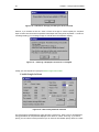
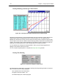
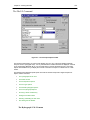
Hydrology - Lag and Route
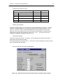
Figure 2-15 – Data input for the Lag and Route command
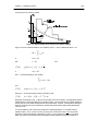
Calculating the runoff from a large catchment (e.g. more than 100 hectares or 250 acres) is complicated
by the fact that the travel time of the runoff from sub-areas close to the outflow point will be much shorter
than from sub-areas at the furthest upstream regions of the watershed or sewer-shed. This causes the
incremental runoff hydrographs to have peak flows which are spread over time with the result that the
peak outflow is significantly less than the sum of the constituent peaks.
18
Chapter 2 – Structure and Scope of the Main menu
MIDUSS 98 incorporates a Lag and Route procedure which can provide an approximation to this effect.
Although it is empirical and thus only approximate it is preferable than using unrealistically long overland
flow lengths to provide an appropriate amount of peak attenuation. The method assumes that a
hypothetical linear channel and linear reservoir are located at the outflow point of the catchment. The
result is that the peak outflow is lagged in time and reduced in value.
The key to success is, of course to assign the correct lag times to the linear channel and linear reservoir.
The empirical procedure used is described in Chapter 7 Hydrological Theory. The procedure to use the
Lag and Route command is described in Chapter 3 Hydrology Used in MIDUSS 98, Lag and Route
Command .
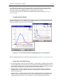
Hydrology - Baseflow
Figure 2-16 – Adding a constant baseflow to the Inflow hydrograph
Even if the first element of the effective rainfall is finite, the direct runoff hydrograph starts with an initial
value of zero. If you want to simulate the effect of baseflow in a drainage system you can add a constant
flow value to the Inflow hydrograph.
The Baseflow command is enabled only after an Inflow hydrograph has been generated.
Refer to Chapter 3 Hydrology Used in MIDUSS 98 - Baseflow Command for more details.
Hydrology - Retrieving the Previous Storm
Figure 2-17 – The Hydrology menu after specifying a second storm
If you specify a second design storm during a MIDUSS 98 design session the previous storm hyetograph
will be overwritten with the new storm and this new hyetograph will be used for all future uses of the
Catchment command. However the first storm is kept in memory and can be recovered if required.
Accepting the second storm causes the Hydrology menu to have a new item added at the bottom as
illustrated in Figure 2- 17. Using the Retrieve Storm command causes the first storm to be restored but
the second storm is not saved. This command may be useful in two cases.
Chapter 2 – Structure and Scope of the Main Menu
•
You mistakenly define a new storm
•
You need to change the storm for only a few sub-catchments.
19
If you need to switch between two or more storms several times the simplest solution is to store the
hyetograph as a file. See the File Input/Output command in Chapter 6 Working with Files.
The Hydrograph Menu
Figure 2-18 – Hydrograph operations available in MIDUSS 98
This menu item allows you to manipulate hydrographs in a number of different situations. Not all of the
options may be enabled unless the appropriate pre-requisites are satisfied, e.g. the Combine command
is available only after an Output hydrograph has been generated.
Hydrograph Undo
This menu item is enabled only if a hydrograph has been written to the backup hydrograph. This is done
in a number of instances to allow you to reverse an operation. For example, you may have used the Add
Runoff command which causes the Runoff hydrograph to be added to the current inflow hydrograph.
You may wish to 'Undo' this action and restore the previous Inflow hydrograph. In such a case, the Undo
menu item will be enabled and pressing this command will restore the Inflow hydrograph to its previous
state.
Hydrograph Start
Figure 2-19 – The Hydrograph/Start item offers two choices
20
Chapter 2 – Structure and Scope of the Main menu
The Start menu item has two subsidiary choices to let you either:
•
set the Inflow hydrograph to zero or
•
edit the current inflow hydrograph.
The first option is generally used after you have stored an outflow hydrograph at a Junction node (by
using the Combine command) and therefore wish to start a new tributary of the drainage network. If you
fail to zero the Inflow hydrograph, the runoff from the first catchment of the new tributary will be added to
the furthest downstream Inflow hydrograph of the previous branch.
The second option in the Start command is less commonly used but may be useful to input a hydrograph
which represents observed data for comparison with a simulated hydrograph. Alternatively, you may
wish to input a hydrograph obtained by use of another model.
Hydrograph Add Runoff
This command causes the Runoff hydrograph to be added to the current Inflow hydrograph so that a new
pipe, channel or other drainage element can be designed to carry the increased flow. A message box is
displayed to inform you what action has been taken and a new record is added to the database displayed
in the Peak Flows table in the bottom right corner of the MIDUSS 98 window showing the change in the
peak of the Inflow hydrograph.
Figure 2-20 – Hydrograph operations provide an explanatory message
Note that in general the time to peak for the Runoff and Inflow hydrographs will not be the same. For this
reason, the peak of the sum of two hydrographs will usually be less than the sum of the individual peaks.
The original value of the Inflow hydrograph is stored in the Backup hydrograph array and the Undo
command is enabled. This allows you to reverse the action and restore the Inflow to its previous state.
See the Hydrograph - Undo command for details.
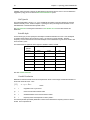
Hydrograph Next Link
This command causes the Outflow hydrograph to be copied to the Inflow hydrograph overwriting the
previous contents. This command is used when an Outflow hydrograph has been created by a routing
process and you want to continue downstream to the next reach of conduit or channel, etc.
Once the Inflow has been updated in this way you may wish to define another catchment area and add
the runoff from this area to the inflow before continuing with the design of the drainage network. Thus a
typical sequence of commands might be represented by the following fragment of the peak flow summary
table.
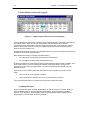
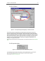
Chapter 2 – Structure and Scope of the Main Menu
Figure 2-21 – The peak flow summary table after the Add Runoff command.
As with other hydrograph operations, the Inflow hydrograph is stored in the Backup hydrograph before it
is overwritten thus allowing you to use the Undo command to reverse the operation and restore the
Inflow to its original state.
Hydrograph Combine
Figure 2-22 – The Hydrograph/Combine form offers step-by-step advice
The Combine command is used to store or accumulate an Outflow hydrograph at a junction node. The
first time you store a hydrograph at a junction node, the peak flow is shown in the Junction or temporary
column of the Peak Flows table, the hydrograph is stored in the current Junction or Temporary array and
a file is created with the name Hydnnnnn.jnc where 'nnnnn' is the number of the junction node.
The next logical step is to clear out or set to zero the Inflow hydrograph in preparation for computing the
flow in another branch of the drainage network. This branch will eventually terminate at the same
junction node or at a different one. If it is added to the same node, the peak flow, the Junction
hydrograph and the Junction hydrograph file are all updated.
If a different Junction node is used the peak flow and the Junction hydrograph are overwritten and a new
Junction hydrograph file is created. Since junction flows are always stored as a file it is possible to have
21
22
Chapter 2 – Structure and Scope of the Main menu
any number of Junctions nodes active at one time
A more detailed description of the use of Junction nodes is provided in Chapter 5 – Hydrograph
Manipulation, The Combine Command.
Hydrograph Confluence
The Confluence command is used in conjunction with the Combine command and allows you to recover
the accumulated flow at a junction node and copy it to the Inflow hydrograph, overwriting the previous
contents. In this way, the command lets you continue the design of the drainage network downstream of
a junction node.
The table in Figure 2-23 has been copied from the summary of peak flows and shows a design sequence
in which two tributaries are accumulated at a confluence node.
Figure 2-23 – Sequence of operations adding two branches at a Junction
In carrying out the operation the Inflow hydrograph is first copied to the Backup hydrograph to allow use
of the Undo command, the junction flow in the Peak Flows window is set to zero, the Junction array is set
to zero and the Junction file is deleted. All of these actions can be reversed if you subsequently use the
Undo command.
Before continuing with the design of the drainage network downstream of the junction node you may
define a local catchment and add the runoff to the inflow if this is appropriate.
Hydrograph Copy To Outflow
This command causes the current inflow hydrograph to be copied to the Outflow hydrograph overwriting
the current contents. This may be useful if the current inflow is to be added to a new or existing junction
node without the need to use a Design option such as the Pond command or the Pipe & Route
commands.
The action can be reversed by means of the Hydrograph/Undo command.
Chapter 2 – Structure and Scope of the Main Menu
23
Hydrograph Refresh
This command is enabled if there are one or more junction files in the current Job directory and is
intended to let the user selectively delete junction files which are no longer required.
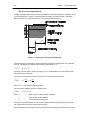
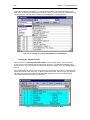
Hydrograph File Input-Output
Figure 2-24 – The File I/O command offers many options.
During a MIDUSS 98 session you will create a number of hydrographs at different points throughout the
drainage network. Also, the storm hyetograph and the effective rainfall on pervious and impervious
surfaces are created. You may wish to save some of this data in the form of files either for subsequent
plotting or analysis or for use in a subsequent design session. The File Input-Output command lets you
do this.
All of the files will be stored in the current Job directory. For this reason, if you expect to be saving files it
is strongly recommended that you specify an Output file in a Job specific directory to avoid storing this
data in the Miduss98 directory.
Each file contains six records in the header section to store information such as a description, the units
employed and the time step, the peak value and the number of elements in the file.
24
Chapter 2 – Structure and Scope of the Main menu
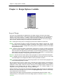
The Design Menu
Figure 2-25 – Design tools available in MIDUSS 98
The Design functions are generally all enabled once an Inflow hydrograph has been created. One
exception is the Route command which requires that a Pipe or Channel conduit has been designed.
Another difference is that the Pipe and Channel commands are always enabled to allow you to enter a
flow value and design a pipe or channel for that flow without having to define a storm and generate a flow
hydrograph.
Design Design-Log
Figure 2-26 – A typical Design Log during a Pond design
Each of the six options in the Design menu causes a Design Log window to be opened in the top right
corner of the screen. This is used to record a summary of the steps taken during a design process. For
simple elements such as a pipe design, the data requirements are limited to the roughness and to
successive trials with different diameters and/or slopes. However, for a more complex drainage element
such as a detention pond, there are many options which can be employed and the trial and error process
can be complicated. In these cases the Design Log can be useful as a reference to earlier trials and also
serves as a reminder should you be interrupted during the design process.
The current design log can be printed out at any time for convenience of reference.
Chapter 2 – Structure and Scope of the Main Menu
25
At the end of the design of each element the Design Log is copied to a file which can be saved or printed
out at the end of the MIDUSS 98 session. The total Design Log can also be viewed by using the
Show/Design log menu item. Refer to the Show menu for more details.
Design Pipe
The Pipe command lets you design a pipe to carry the peak flow of the current Inflow hydrograph. If no
hydrograph has been calculated you can specify a desired flow directly by entering it in the text box. For
the specified peak flow you will be shown a table of diameters, gradients and average velocities which
represent feasible designs. You can either choose one of these diameter-gradient pairs by double
clicking on a row in the table or you can enter explicit values for diameter and gradient.
MIDUSS 98 carries out a uniform flow analysis and reports the actual depth and velocity and also the
critical depth. You can experiment by changing either the pipe roughness (i.e. the Manning 'n') or the
diameter or gradient and press the [Design] button to see the results. When satisfied with the design
press the [Accept] button to copy the data and results to the Output file.
Design Channel
MIDUSS 98 lets you design channels with two types of cross-section to carry the current peak flow in the
Inflow hydrograph. If no hydrograph has been calculated you can enter a flow value directly by entering it
in the text box. The cross-section can be:
(1)
A general trapezoidal shape defined by a base width and left and right sideslopes.
(2)
An arbitrary shape defined by up to 50 pairs of coordinates.
In both cases a table of depth, gradient, velocity values is displayed which represent feasible designs.
You can select from this list by double clicking on a row of the table or you can specify a total depth and
gradient explicitly. MIDUSS 98 carries out a uniform flow analysis for the given flow, roughness and
geometry and reports the depth of flow, the average velocity and the critical depth in the channel.
You can experiment by changing the data and pressing the [Design] button. When satisfied, press the
[Accept] button to save the data and results to the output file.
Design Route
Once a drainage conduit has been designed - either a pipe or channel - you can route the Inflow
hydrograph through a reach of specified length to obtain the Outflow hydrograph at the downstream end.
For each trial design MIDUSS 98 checks that the time step and reach length are acceptable to ensure
stability in the routing process. If the time step is too long it will be reduced to an appropriate submultiple. If the reach length is too long it also will be subdivided. In both cases the information is
reported on the screen but no further action is required by the user.
The result of the routing operation is displayed in both graphical and tabular form. Once you are satisfied
with the result you can press the [Accept] button and the peak flow summary table will be updated.
Design Pond
MIDUSS 98 helps you to design a detention pond to achieve a desired reduction in the peak flow of a
hydrograph. The current peak flow and the total volume of the inflow hydrograph are reported and you
are prompted to specify the desired peak outflow. MIDUSS 98 estimates the maximum storage
requirement to achieve this.
26
Chapter 2 – Structure and Scope of the Main menu
The storage routing through the pond requires a table of values defining the outflow discharge and the
storage volume corresponding to a range of stage or depth levels. You can enter this data directly into
the grid if you wish, but it is usually easier to use some of the features of the Pond command to automate
this process.
The outflow control can be designed using multiple orifices and weir controls. The Stage - Storage
values can be estimated for different types of storage facility. These may be a multi-stage pond with an
idealized rectangular plan shape and different side slopes in each stage; one or more "super-pipes" or
oversized storm sewers; wedge storage formed on graded parking lots; or a combination of these types
of storage.
Rooftop storage can also be modelled to simulate controlled flow from the roof of a commercial
development.
Design Trench
The Trench command lets you proportion an exfiltration trench to provide underground storage for flow
peak attenuation and also to promote return of runoff to the groundwater. The trench usually consists of
a trench of roughly trapezoidal cross-section filled with clear stone with a voids ratio of around 40% and
with one or more perforated pipes to distribute the inflow along the length of the trench.
The exfiltration trench splits the inflow hydrograph into two components. One of these is the flow which
exfiltrates into the ground water; the balance of the inflow is transmitted as an outflow hydrograph.
Obviously an exfiltration trench requires reasonable porosity of the soil and a water table below the
trench invert in order to operate effectively.
The design involves several steps including definition of the trench and soil characteristics, definition of
the number, size and type of pipes in the trench and description of the outflow control device comprising
orifice and weir controls as used in the Pond command.
More detailed information is contained in Chapter 4 Design Options Available, Design Exfiltration Trench.
Design Diversion
A diversion structure allows the inflow hydrograph to be split into two separate components, the outflow
hydrograph and the diverted flow hydrograph. Below a user-specified threshold flow all of the inflow will
be transmitted to the outflow hydrograph. When the inflow exceeds the threshold value, the excess is
divided in proportion to a specified fraction.
For example, if the inflow is 25 cfs and the threshold is 5 cfs the excess flow is 20 cfs. Now if the fraction
F = 0.8 meaning that 80% of the excess flow is diverted the diverted flow will be 16 cfs and the outflow
will be 9 cfs.
Instead of specifying the diverted fraction F you can define this implicitly by specifying the desired peak
outflow. MIDUSS 98 will then work out the necessary fraction to be diverted.
The diverted flow hydrograph is written to a file so that it may be recovered at a later time and used to
design the necessary conduit or channel.
Use of the diversion command is the only instance in which the topology of the network changes from a
tree to a circuited network.
Refer to Chapter 4 Design Options Available, Diversion Structure Design for more information.
Chapter 2 – Structure and Scope of the Main Menu
27
The Show Menu
Figure 2-27 – Options available for displaying your results
The options in this menu allow you to display the results of your hydrologic modelling and design.
Results for inclusion in a report can be displayed in tabular format or in graphical form. For each of these
choices you can specify the particular data items to be displayed. The menu items are not enabled until
there is data available to be displayed.
Show Output File
This command causes the Microsoft program Notepad to be opened with the current Outflow file. You
can review the contents of the file, print all or part of the file or save it with a name other than that initially
assigned to the file. (You can use the same filename but in a different directory).
However, you cannot make changes to the file since it must be re-opened when the Notepad window is
closed.
Show Design Log
This command lets you review the contents of the current Design Log file. The Microsoft editor Notepad
is opened with the current Design Log. As with the Output file, you can review it, print it or save it with a
different path or name but you cannot change the contents.
When the Notepad window is closed the Design Log file is re-opened in Append mode so that additional
records written to the Design Log will be added.
Show Flow Peaks
If for some reason you have closed the window showing the summary of flow peaks (usually in the lower
right corner of the MIDUSS 98 window) this command will restore the table and refresh the values. The
records for each row of the table are contained in a text file called Qpeaks.txt which resides in the
Miduss98 directory. Normally you will have no need to refer to this but should you wish to do so it can be
viewed and printed or saved by another name or path by using the Microsoft editor Notepad which can be
run from the Tools menu or from the desktop after the MIDUSS 98 session has been completed.
28
Chapter 2 – Structure and Scope of the Main menu
Show Tabulate
Figure 2-28 – Some of the options available with the Show/Tabulate command
A tabular display of each rainfall hyetograph or flow hydrograph is displayed - usually in the lower left
corner of the MIDUSS 98 window - as the MIDUSS 98 session proceeds. This command lets you
display the table for any of the three hyetographs or four hydrograph arrays which are currently in use.
Show Quick Graph
With each step of the MIDUSS 98 session a graphical display is opened in the top right corner of the
MIDUSS 98 window. This command lets you open a similar graphical window to display any of the
current 3 rainfall hyetographs or 4 flow hydrographs.
Figure 2-29 – Some of the Options available with the Show/Quick Graph command
Show Graph
This command lets you construct a graphical display comprising several hydrographs and hyetographs.
If a rainfall hyetograph is plotted first it may be drawn either on the bottom axis or along the top edge of
the plotting window.
However, if one or more hydrographs have been plotted, the addition of a hyetograph will be
automatically placed on the top edge with the scale reading downwards.
Chapter 2 – Structure and Scope of the Main Menu
29
The scale for both time and ordinate value can be set when the first object is plotted but subsequent
objects are plotted to the same scale.
You can annotate the graphic by adding text, arrows, lines, rectangles or circles.
The graphic can be saved as a file or a previously saved graphic file can be imported to the empty
graphic window. To conveniently store the graphic for addition of other objects later in the MIDUSS 98
session the form can be iconized from a menu item and restored by re-invoking the Show/Graph
command.
The colour, line thickness and fill pattern can be selected by the user. The preferred styles are
automatically saved as default values when the MIDUSS 98 session is ended.
The Automatic Menu
Figure 2-30 – Commands available for running in Automatic mode
The four options in this menu allow you to run MIDUSS 98 in Automatic mode. When MIDUSS 98 runs
in normal, Manual mode the commands, data and some of the results are copied to an output file. To
use this file for input in Automatic mode it must be converted into a Database file. The data base can be
reviewed and edited prior to running in Automatic mode.
Automatic - Create Input Database
When running in Automatic mode MIDUSS 98 uses a specially created Database file called Miduss.Mdb
which resides in the Miduss98 directory. This file can be created from an existing Output file by means of
this menu command.
When you use this command a standard File Open dialogue box is opened. You should navigate to the
appropriate directory and select the Output file which you wish to use in creating the Input Database file.
During processing a small window opens to show the number of records processed and the number of
commands read.
You can immediately make use of the Edit Miduss.Mdb Database or Run Miduss.Mdb commands.
See Chapter 10 – Running MIDUSS 98 in Automatic Mode for more details.
Automatic- Edit Miduss.Mdb Database
This menu command lets you review and edit the contents of the current Input Database file 'Miduss.Mdb'
in the Miduss98 directory. Editing is limited to changing data values in a field of a particular record. It is
not possible to insert new commands in the Database using this command.
If you want to make major changes such as adding or deleting an entire command you can do this by
interrupting a run in Automatic mode and entering the necessary manual commands. You may do this
also by editing the Output file in a text editor such as Notepad. However, you should attempt such editing
only after you are fully conversant with the sequence and format of the required data.
30
Chapter 2 – Structure and Scope of the Main menu
See Chapter 10 – Running MIDUSS 98 in Automatic Mode for more details.
Automatic - Run Miduss.Mdb
This command causes a control panel to be displayed which contains a grid and several command
buttons. The grid shows the current contents of the database file Miduss.Mdb
The command buttons let you run the input database automatically in three different modes.
(1)
EDIT mode lets you see the result of each command and you may make any changes to
the data prior to pressing the [Accept] key on the command form. Any changes will be
reflected in the new Output file being created.
(2)
STEP mode advances the input file one command at a time but you do not have the
opportunity to make changes to the data.
(3)
RUN mode causes the commands to be processed sequentially without a pause until any
one of the STEP, EDIT or MANUAL buttons is pressed or until the end of file is reached or
until a negative command number is read..
See Chapter 10 – Running MIDUSS 98 in Automatic Mode, Using the Automatic Control Panel for further
details.
Automatic - Enable Control Panel Buttons
Sometimes when running in Automatic mode you may find that all of the command buttons are disabled
or ‘grayed out’. This command allows you to re-enable the command buttons to let you continue in either
automatic or manual mode.
The Tools Menu
Figure 2-31 – Choices available in the Tools menu
The Tools menu provides access to the Microsoft Calculator, the Notepad text editor or the Wordpad
editor from within MIDUSS 98. Other links will be added in future releases for tools such as the IDF
Curve Fit auxiliary program and the Microsoft EXCEL spreadsheet.
In addition, a menu item is provided to let you add comments to the currently defined output file.
Chapter 2 – Structure and Scope of the Main Menu
31
Tools - Add Comment
When you run MIDUSS 98 there is always an Output file, whether one is specified explicitly by the user
in a Job Directory or the default output file 'Default.Out' which resides in the directory C:\Program
Files\Miduss98\. This menu command lets you add explanatory comments to the output file.
You simply type in the text box using normal text editing features such as BackSpace, Delete or mouse
controls. The font used is a uniformly spaced Courier font to allow columns to be aligned if desired. The
text box entry provides automatic word wrap but this may not correspond exactly to the location of new
lines in the output file.
The double quote character cannot be included in a comment and is automatically trapped and converted
to a single quote.
The comment window can be re-sized by dragging the right side or the bottom of the window. The text
entry box will also be re-sized. You can enter as many lines of comment ass you wish. A vertical scroll
bar appears when there are more lines than the text box can display.
The maximum line length which is written to the output file is 60 characters and you cannot use a ‘word’
or string of characters more than 59 characters in length.
Another use for the Add Comment command is to add a visual description to the MIDUSS 98 window
before printing hardcopy of the screen. If you don’t want this added to the output file press [Cancel] to
close the window.
Tools - the Microsoft Calculator
Clicking on this menu item causes the Microsoft Calculator Accessory to be opened. This may be useful
if some hand calculation is required during a MIDUSS 98 session.
When MIDUSS 98 starts up it attempts to locate the directory where Calculator resides and stores this
for later use. However, if the file Calculator.exe cannot be found for any reason you will be prompted to
locate this manually in a standard File Open dialogue box. Once located, the directory will be stored in
the Windows 95 registry for future use.
When you finish using Calculator you should close it in the normal way rather than merely clicking on the
MIDUSS 98 window which will place the Calculator window behind the MIDUSS 98 window and
probably out of sight. This may lead to multiple instances of Calculator being opened simultaneously.
Tools - the Microsoft Notepad editor
This command opens the Microsoft text editor Notepad. You can load, view and edit text files with this
facility. Notice however, that files which are currently in use by MIDUSS 98 - such as the current output
file - cannot be changed. You can, however, print out the file in whole or in part or save it with a different
filename.
When you save a file from Notepad, check to see if Notepad has added the default extension ".txt" to the
filename which you have specified.
When MIDUSS 98 starts up it attempts to locate the directory where Notepad resides and stores this for
later use. However, if the file Notepad.exe cannot be found for any reason you will be prompted to locate
this manually in a standard File Open dialogue box. Once located, the directory will be stored in the
Windows 95 registry for future use.
When you finish using Notepad you should close it in the normal way rather than merely clicking on the
MIDUSS 98 window which will place the Notepad window behind the Miduss98 window and probably out
of sight. This may lead to multiple instances of Notepad being opened simultaneously.
32
Chapter 2 – Structure and Scope of the Main menu
.Tools - the Microsoft Wordpad editor
This command causes the Microsoft text editor Wordpad.exe to be opened. You can load, view and edit
text files with this facility with more flexibility than is possible with Notepad. Notice however, that files
which are currently in use by MIDUSS 98 - such as the current output file - cannot be changed. You
can, however, print out the file in whole or in part or save it with a different filename.
When MIDUSS 98 starts up it attempts to locate the directory where Wordpad resides and stores this for
later use. However, if the file Wordpad.exe cannot be found for any reason you will be prompted to
locate this manually in a standard File Open dialogue box. Once located, the directory will be stored in
the Windows 95 registry for future use.
When you finish using Wordpad you should close it in the normal way rather than merely clicking on the
MIDUSS 98 window which will place the Wordpad window behind the Miduss98 window and probably
out of sight. This may lead to multiple instances of Wordpad being opened simultaneously.
The Windows Menu
Figure 2-32 – You can arrange windows in different ways
The Window menu lets you modify the way the windows are displayed and also lists the windows which
are currently open.
Windows - Cascade
This causes all of the currently open windows to be displayed in the standard Windows cascade style.
Windows - Tile
This causes all of the currently open windows to be displayed in the standard Windows tile arrangement.
Windows - Arrange Icons
Incomplete -Temporary Topic
Windows - Status Bar
This command has the same effect as the Show Status Bar command in the Options menu.
Chapter 2 – Structure and Scope of the Main Menu
The Help Menu
Figure 2-33 – The standard Help menu is available
This menu has the normal choices available in most Windows applications plus one extra item.
Help - Contents
Help - Using Help
Help - Tutorials
Help - About Help for details.
Help - Contents
This command causes the contents of the MIDUSS 98 Help System to be displayed. This follows the
normal standard for Windows 95 Help documents. You can access help in three ways.
(i)
You can double click on a closed volume to expand the contents of that book and search for the
topic of interest.
(ii)
You can search for references to a particular word.
(iii)
Using the '<' and '>' buttons you can browse through the topics in the order in which they appear
in the help documents.
In general the help topics cover the following contents.
•
Chapter 1 - Introduction to MIDUSS 98
•
Chapter 2 - Overview of the Main Menu
•
Chapter 3 - Hydrology Used in MIDUSS 98
•
Chapter 4 - Design Options Available
•
Chapter 5 - Hydrograph Manipulation.
•
Chapter 6 - Working with Files
•
Chapter 7 – Hydrological Theory
•
Chapter 8 - Theory of Hydraulics
•
Chapter 9 - Displaying your Results.
•
Chapter 10 - Running MIDUSS 98 in Automatic Mode
•
Chapter 11 - A Detailed Example
33
34
Chapter 2 – Structure and Scope of the Main menu
Help - Using Help
This menu item opens the standard help files that explain in detail how to make best use of the Windows
95 Help system.
Help - Tutorials
The MIDUSS 98 CD contains a folder called Tutorials which holds a number of audio-visual lessons on
the main features and operations of MIDUSS 98. These can be accessed directly from the CD or from
the Help/Tutorial menu command.
Your computer must have a sound card in order to hear the audio track.
Many of the lessons are taken from the steps in Chapter 11 A Detailed Example.
You can copy the lesson files on to your hard disk if you wish, in order to allow the CD to be stored in
your software repository. Currently the disk space required is close to 150 MB and provides over 100
minutes of lessons.
Help - About Help
This menu command causes a window to display a copyright notice with respect to Miduss98 and details
of the registered user of the program.
Chapter 3 – Hydrology used in MIDUSS 98
35
Chapter 3 - Hydrology used in MIDUSS 98
This part of the MIDUSS 98 Help System describes the hydrology commands used to model the rainfall
runoff process and generate the hydrographs for which your stormwater management facilities will be
designed.
The hydrology incorporated in MIDUSS 98 is based on relatively simple and generally accepted
techniques. There are four commands to control the fundamental operations.
(1)
STORM - This command allows you to define a rainfall hyetograph either of the synthetic, design
type or a historic storm.
You should remember that as an alternative to using the STORM
command, a previously defined rainfall hyetograph may be read in from a disk file, by means of the
FILE Input/Output command.
(2)
CATCHMENT - The Catchment command lets you define a single sub-catchment and computes
the total overland flow hydrograph for the currently defined storm. The runoff hydrographs from the
pervious and impervious areas are computed separately and added to give the total runoff. The
roughness, degree of imperviousness, overland flow length and surface slope of both the pervious
and impervious fraction are defined in this command. In addition you can choose from different
rainfall loss models. The effective rainfall on these two fractions is computed and stored for future
use. Different methods for routing the overland flow are available.
(3)
LAG and ROUTE. - This command is useful for modelling the runoff from very large subcatchments without having to resort to specifying unrealistically long overland flow lengths. The
command computes the lag time in minutes of a hypothetical linear channel and linear reservoir
through which the runoff hydrograph is routed. Typically this results in a smaller, delayed runoff
peak flow.
(4)
BASE FLOW: - This command lets you specify a constant positive value of base flow to be added
to the current inflow hydrograph. The command is enabled only after an inflow hydrograph has
been defined.
This chapter describes how to use these commands and discusses the hydrological techniques in general
terms. More information on the background theory can be found in Chapter 7 – Hydrological Theory. If
you need further information refer to any standard text on the subject. A number of references for this
purpose are provided in Appendix ‘A’. You may also find it useful to subscribe to one or more of the
relevant discussion groups which are available on the Internet.
MIDUSS 98 offers a choice between four alternative methods for routing the overland flow and three
different models for estimating infiltration and rainfall losses. In general these different methods will result
in significantly different results. MIDUSS 98 may therefore be used to compare methods and to examine
the sensitivity of the resulting runoff hydrograph to the methods used. This flexibility means, however, that
the engineer must exercise some care and consistency in the selection of procedures and parameter
values for a particular application.
An important distinction must be made between the three overland flow routing methods which are based
on the notion of effective rainfall and the SWMM Runoff method which uses a surface water budget
approach which computes both runoff and rainfall loss as a function of rainfall. The difference is
particularly noticeable when the runoff from the pervious fraction is significant This is discussed in more
detail in Chapter 7 – Hydrological Theory, Rainfall-Runoff Models..
36
Chapter 3 – Hydrology used in MIDUSS 98
Storm Command
Figure 3-1 – Five design storms are available
The rainfall hyetograph can be defined in five ways using this command. You may choose to define
either:
or
(1)
a synthetic design storm from four different types available,
(2)
a historic rainfall record based on observed data.
The form for the Storm command offers five alternate Tabs and selection is made by clicking on one of
these. Select from the first four for a design storm or choose the fifth option for a historic storm.
Chicago Storm Hyetograph
Huff Storm
Mass Rainfall Distribution
Canadian AES 1-hour Storm
Historic Storm
After you have defined or accepted the parameters for the selected storm type you can press the
[Display] command button to compute the storm hyetograph. This is displayed in both a graphical and
tabular form. Since these features are common to all types of design storm they are described first.
Refer to Graphical Display of the Storm to see a typical graph of a Chicago storm.
Refer to Tabular Display of the Storm Hyetograph to see the corresponding table of rainfall intensities.
You can experiment by changing one or more of the parameter values and press [Display] again. When
you are satisfied with the design storm you should press the [Accept] command button to store the
hyetograph. The design storm will remain unchanged until you change it by a second use of the Storm
command or by importing a hyetograph file.
The description of each of the design storms referenced above describes how these options can be used.
A more detailed description of some of the design storm options is contained in Chapter 7 Hydrological
Theory.
Chapter 3 – Hydrology used in MIDUSS 98
37
Graphical Display of the Storm
Figure 3-2 – A typical plot of the design storm.
A graph of the storm hyetograph is presented when you press the [Display] command button. The graph
illustrated in Figure 3-2 is for a Chicago hyetograph. You can test the sensitivity of the storm to changes
in any of the parameters by altering the data and pressing [Display] again. The storm will not be stored
until the [Accept] command button is pressed.
A similar graphical display is also shown for hydrographs following any of the commands which result in
some change in the hydrograph data.
When you move the mouse pointer over the graph a small window displays the time and either a rainfall
intensity or a hydrograph flow value corresponding to the position of the vertical cross-hair. If you hold
down the right Mouse button a pair of cross-hairs will follow the mouse pointer. The position of the
horizontal cross-hair has no significance but the vertical cross-hair should intersect the time axis at the
time value shown in the small data window.
You can position the graph window by clicking on the title bar and dragging the window to a new location.
You can also resize the graph window by dragging any corner of the graph window. The graph is
automatically scaled to fit the window. The graph window can also be shown in full screen mode or
reduced to an icon by clicking on the window size controls at the top-right corner of the window.
If you click with the primary mouse button anywhere in the plot area, the window is restored to its default
size and position in the upper right corner of the MIDUSS 98 window.
38
Chapter 3 – Hydrology used in MIDUSS 98
Tabular Display of Storm Hyetograph
Figure 3-3 – A tabular display of Mass Curve storm hyetograph.
When the [Display] command button is pressed a table of rainfall intensities is displayed in the lower left
corner of the screen. When you move the mouse pointer over the table, the time in minutes
corresponding to the cell beneath the pointer is displayed in the top-right corner of the grid. The Spin
Button on the top right corner lets you vary the number of figures after the decimal point between a
minimum of 0 and a maximum of 5.
A similar tabular display is also shown for hydrographs following any of the commands which result in the
generation of a new set of hydrograph data.
Basic statistics are shown in the header of the table defining:
•
For hyetographs, the total depth of rainfall and the peak intensity.
•
For hydrographs, the total volume and the peak flow rate.
By altering the data for the command and pressing the [Display] button again the table is updated. In the
Storm command, this is useful for checking the sensitivity of the design storm to changes in the
parameters or even in the type of design storm. For other commands a similar capability exists for
sensitivity analysis.
If the number of rows of data is greater than the number of rows in the table you can do one of two
things.
•
use the scroll bar on the right side of the table
•
click on and drag the top edge of the form to increase the height of the form.
The second method is useful if you need to print out the entire contents of the table.
Accepting the Storm
The [Accept] command button is initially disabled when you first use the Storm command. When you
press the [Display] button to show the graph and tabular display, the [Accept] button is enabled.
However, if you change any of the parameter values, the [Accept] button is again disabled until the
[Display] button is used to refresh the storm hyetograph.
Chapter 3 – Hydrology used in MIDUSS 98
39
Figure 3-4 – The peak flow summary table with a single record.
Once you are satisfied with the storm you can cause it to be stored by pressing the [Accept] button. The
graph and tabular display windows are closed and the small summary window shown in Figure 3-4 is
displayed in the lower right corner of the screen. This table will be updated with hydrograph information
as you define sub-catchments and design components. For this initial display only the storm has been
defined and no runoff hydrographs have been generated.
Chicago Hyetograph
Figure 3-5 – The Chicago storm tab of the Storm command
When you select the Chicago hyetograph tab the data entry form shown in Figure 3-5 is displayed. The
synthetic hyetograph computed by the Chicago method is based on the parameters of an assumed
Intensity - Duration - Frequency (IDF) relationship, i.e.
i=
[3.1]
where
a
(td + b )c
i
=
average rainfall intensity (mm/hr or inch/hr)
td
=
storm duration (minutes)
a,b,c
=
constants dependent on the units employed and the return frequency of the storm.
40
Chapter 3 – Hydrology used in MIDUSS 98
The asymmetry of the hyetograph is described by a parameter r (where 0 <
point within the storm duration td at which the rainfall intensity is a maximum.
r < 1) which defines that
In hypertext you can click on any of the data entry text boxes in Figure 3-5 for a brief explanation of each
parameter; in hardcopy the same information is given below. When data has been entered press the
[Display] command button to see a graphical plot of the storm hyetograph and a table of rainfall
intensities. You can change any value and press [Display] again to see the effect of the change. When
you are satisfied with the storm, press [Accept] to define the storm.
Although widely used in North America, the Chicago storm has been criticized because it combines the
characteristics of many different events and does not necessarily provide a reasonable simulation of an
actual storm. In particular, the peak intensity is very sensitive to the time step employed. For that reason
some engineers prefer to use a multiple of the time step in the vicinity of the peak. The time step
multiplier can be used for this purpose. The volume of rainfall is unaffected but the peak intensity is
significantly reduced. The best way to understand this is to experiment by increasing the multiplier to 2 or
3 and press [Display] to see the effect.
If you have access to data defining either depth or average intensity for different times, you can use the
IDFCurveFit program to estimate the values of a, b and c which give the closest fit to the observed IDF
data.
The 'a' coefficient
The value of the 'a' coefficient depends on (i) the return interval in years of the storm and (ii) the system
of units being used. e.g.
Years
Metric
Imperial
2
250
10
5
400
17
10
700
25
25
950
36
50
1250
50
100
1800
75
Use these default values only as a last resort.
The b-constant
This constant in minutes is used to make the log-log correlation as linear as possible. Typical values
range from 2 to 12 minutes. A value of zero for this parameter represents a special case of the IDF
equation where
[3.2]
i=
a
tdc
.
In general, this results in poor agreement between observed values of intensity and duration and those
represented by the IDF equation.
The c-exponent
This parameter is usually less than 1.0 and is obtained in the process of fitting the data to the power
expression. Values are usually in the range 0.75 to 1.0
Chapter 3 – Hydrology used in MIDUSS 98
41
The r-peak fraction
This parameter is the fraction of the storm duration to the point of maximum rainfall intensity (e.g. in
Figure 3-2 the value of r is 0.4). Values are usually in the range 0.25 to 0.6 but any value less than 1.0
may be used. Notice that on pervious surfaces a high (i.e. late) value of r will result in a higher runoff
peak since the ground tends to be more saturated when the peak intensity occurs.
Duration
This defines the duration of the storm in minutes. It must be not greater than the maximum storm
duration defined in the time parameters. Usually some multiple of the time step is used.
Time step multiplier
If a very small time step is used with the Chicago hyetograph it can result in a very high peak rainfall
intensity. You can use an integer multiplier to use a small time step but avoid the unrealistically high
peak. Experiment to see the difference.
Huff Rainfall Distribution
Figure 3-6 – The Huff distribution tab of the Storm command
Selection of the Huff Distribution tab on the Storm command form causes the form shown in Figure 3-6 to
be displayed. The non-dimensional rainfall distribution patterns suggested by Huff were divided into four
groups in which the peak intensity occurs in the first, second, third or fourth quarter of the storm duration.
Within each group the distribution was plotted for different probabilities of occurrence. MIDUSS 98 uses
the median curve for each of the four quartile distributions. (See Chapter 7 Hydrological Theory;
Derivation of the Huff Storm).
To define a storm of this type you must provide values for the total depth and duration of the storm and
select the quartile distribution required. Refer to the topics which follow for a brief explanation of each
parameter. When data has been entered press the [Display] command button to see a graphical plot of
the storm hyetograph and a table of rainfall intensities. You can change any parameter value and press
[Display] again to see the effect of the change. When you are satisfied with the storm, press [Accept] to
define the storm.
42
Chapter 3 – Hydrology used in MIDUSS 98
Canadian users who want to employ the Atmospheric Environment Service 1-hour of 12-hour distribution
suggested by Hogg can do so with the Mass Rainfall Distribution option.
Huff Quartile
The Huff quartile takes a value of 1, 2, 3 or 4 and defines the quartile of the storm duration in which the
maximum intensity occurs. Refer to Chapter 7 Hydrological Theory for background information on the
Huff distribution or the dimensionless quartile curves.
See Huff Distribution for background information or Huff Quartile Curves for the data used for this
distribution.
Rainfall depth
For this storm type you must specify the total depth of rainfall in millimetres or inches. This will depend
on climatic factors and the return interval in years. It is common to use the Intensity - Duration Frequency curve for the area from which the total depth can be estimated for a given storm duration and
return interval in years.
The values below are typical for some regions in Southern Ontario, Canada.
Return
period
Depth
% of 5 year
(years)
(mm)
(inch)
(%)
2
38.0
1.50
78%
5
48.6
1.90
100%
10
55.7
2.20
115%
25
64.5
2.55
133%
50
71.1
2.80
146%
100
77.6
3.05
160%
See also Gumbel Distribution
Gumbel Distribution
Estimates for extreme rainfall events can be expressed in terms of the average and standard deviation of
the annual maximum series. Thus:
xT = µ x + KT σ x
[3.3]
where
xT
=
magnitude of the T year event
µX
=
mean of the annual maximum series
σX
=
standard deviation of the annual maximum series
KT
=
frequency factor which depends on return period T
The Gumbel (double exponential) distribution is often used to describe the frequency factor for extreme
rainfall. This is expressed as:
Chapter 3 – Hydrology used in MIDUSS 98
KT =
[3.4]
43
− 6
T
0.5772 + ln . ln
T −1
π
e.g.
T (years)
2
5
10
25
50
100
K
0.164
0.719
1.305
2.044
2.592
3.137
Values for the mean and standard deviation of the annual maximum series can often be estimated from
rainfall frequency maps.
Mass Rainfall Distribution
Figure 3-7 – The Mass Curve distribution tab of the Storm command
MIDUSS 98 contains a number of files with the extension '.mrd' which stands for Mass Rainfall
Distribution. These files reside in the Miduss98 directory (typically C:|Program Files\Miduss97\..). You
can use one of these pre-defined patterns or create a special one for your own use to define a
customized non-dimensional mass rainfall distribution curve similar to the patterns used for the Huff
storms.
The data form shown above is opened when you select this option. The default location of the *.mrd files
is indicated by the Drive (e.g. C:\) and Directory (e.g. C:\Program Files\Miduss97\) and all files with the
extension .mrd are listed in the Files List box. (Hint: If the file List box shows ‘All Files’, double click on
the drive and then the directory to show only files with the extension *.mrd)
By selecting (i.e. clicking on) one of the files a brief description is displayed below the list box. In addition
to the selected non-dimensional distribution you must specify the total depth and duration for the storm.
Refer to the topics below. When data has been entered press the [Display] command button to see a
graphical plot of the storm hyetograph and a table of rainfall intensities. You can change any of the
values or the distribution pattern and press [Display] again to see the effect of the change. When you are
44
Chapter 3 – Hydrology used in MIDUSS 98
satisfied with the storm, press [Accept] to define the storm.
Irrespective of the number of points used to describe the distribution, the rainfall intensities are
discretized in terms of the time step defined for the MIDUSS 98 session using linear interpolation. The
interpolated values are then scaled up by the total depth of rainfall. More details are provided in Chapter
7 Hydrological Theory. Derivation of the User Defined Distribution.
Drive for *.MRD file
When you install MIDUSS 98 all the files of type *.MRD are located in the Miduss98 directory. If this is
typically C:\Program Files\Miduss98\ then the Drive for the *.MRD files will be 'C:' If you create special
mass rainfall distribution files - either an edited copy of the pre-defined ones, or a customized one of your
own choosing - you may wish to store these in a particular job directory. You can use the Drive list box to
navigate to where your *.MRD files are located.
Directory for *.MRD file
When you install MIDUSS 98 all the files of type *.MRD are located in the Miduss98 directory. If this is
typically C:\Program Files\Miduss98\ then the Directory for the *.MRD files will be 'C:\Program
Files\Miduss97\'. If you create special mass rainfall distribution files you may wish to store these in a
particular Job directory. You can use the Directory list box to navigate to where your *.MRD files are
located.
Select *.MRD file
Once the drive and directory of the path have been selected you can click on the particular *.MRD file to
be used. The description in the text box below helps to ensure you have made the right choice. The file
will not be processed until you press the [Display] command button. Note that the [Display] button is not
enabled until a file has been selected.
Customized *.MRD files
If you create a customized mass rainfall distribution file you should copy the format of one of the predefined files as illustrated below
SCS 6 hour distribution
# 1 - Description
51
# 2 - Number of values N
0.000
# 3 - Initial zero value
0.008
0.016
Intermediate values
0.024
defining (N-1)
0.032
increments.
0.040
:
You can use
0.976
any number of
0.984
points > 2.
0.992
1.0
# N+2 - Final value of 1.0
Chapter 3 – Hydrology used in MIDUSS 98
45
Canadian AES 1-hour Storm
Figure 3-8 – The Canadian AES tab of the Storm command
The form shown in Figure 3-8 is used to define a simple two parameter design storm which has a linear
rising portion followed by an exponentially decreasing curve. The possibility of reversing the linear and
exponential segments is suggested in the original publication (Watt et al) but this option is not currently
supported in MIDUSS 98. A definition sketch is shown in Chapter 7 Hydrological Theory, Canadian 1hour storm derivation
The parameter values required for this option are the depth (mm or inches) and duration (minutes) of the
rainfall the time to peak intensity (minutes) and the decay coefficient K.
You should note that the proposal by Watt et al is intended to be used only for 1-hour storms since the
data used for the work was limited to this duration. However, MIDUSS 98 allows you to define other
values of the duration. Be careful if suggested values for the time to peak are taken from the original
reference since these are intended specifically for 60 minute storms. For that reason, suggested values
in Chapter 7 Hydrological Theory, ‘Suggested tp values for locations in Canada’ show time to peak in
minutes and also as a fraction of the duration but care should be taken in using these.
When the data has been entered press the [Display] command button to see a graphical plot of the storm
hyetograph and a table of rainfall intensities. You can change any of the values and press [Display]
again to see the effect of the change. When you are satisfied with the storm, press [Accept] to define the
storm.
46
Chapter 3 – Hydrology used in MIDUSS 98
AES Time to Peak
Suggested values of time to peak are intended for 60 minute storms. For other values of duration use the
values of Tp /Duration with caution.
Location
Tp (minutes)
Tp/
Duration
Yukon
20
0.33
B.C.(coast)
28
0.47
B.C.(interior), Prince George
13
0.22
Alberta
17-18
0.29
Saskatchewan
23-24
0.39
Manitoba (Brandon, Churchill)
31
0.52
Manitoba (Winnipeg)
25
0.42
Ontario (Timmins, Thunder Bay)
24-25
0.41
Ontario (Ottawa, Kingston, Windsor)
26-27
0.44
Ontario (Toronto, Sudbury)
21
0.35
Quebec (Montreal)
27
0.45
Quebec (Val D'Or, Quebec City)
23
0.38
New Brunswick (Fredericton)
17
0.28
Nova Scotia, Newfoundland
26-28
0.45
AES Decay factor
Values of the decay coefficient taken from the original publication are shown below.
Province
K value
B.C.(coastal region)
5
Yukon, New Brunswick, Nova Scotia,
Newfoundland
6
B.C.(interior), Alberta, Saskatchewan, Manitoba,
Ontario, Quebec
7
Chapter 3 – Hydrology used in MIDUSS 98
47
Historic Storm
Figure 3-9 – The Historic storm tab of the Storm command
This storm option lets you define an observed or historic rainfall event. The form illustrated here prompts
you to specify the duration in minutes. Depth, intensity and distribution are defined by entering intensity
values in a Table that is opened when you press the [Display] button.
If you set a check mark in the box labeled 'Check to set rainfall to zero' the table will be opened with all
values set to zero. Otherwise, the intensity values for the currently defined storm are copied into the
table where they can be edited. Notice that when you are using any of the other four options in the Storm
command, the rainfall intensities displayed do not become the "currently defined storm" until you have
pressed the [Accept] button. Thus, if you wish to generate (say) a 3rd quartile Huff storm and then edit it
using the Historic storm option you must invoke the Storm command twice; once to create and save the
Huff storm and a second time to import it into the Historic storm table for editing.
Figure 3-10 – The Historic storm data entry grid
The table shown above was generated by first creating and 'Accepting' a 3rd quartile Huff storm with a
duration of 120 minutes and a total depth of 50 mm. Then the Storm command was used with the
Historic option for a storm duration of 180 minutes and with the 'Check to set rainfall to zero' checkbox left
empty (unchecked). Note the extra 12 cells (60 minutes) with zero values.
You can navigate around the table using the arrow keys or by clicking the mouse pointer on a cell of the
table. You will notice a slightly heavier outline around the selected cell. You can type a new value into
the current cell and move to the next cell with an arrow key. This will:
48
Chapter 3 – Hydrology used in MIDUSS 98
- overwrite the cell contents
- change the total depth in the table and the peak intensity if the new value is large enough.
- change the total depth in the Storm/Historic form
- update the graphic display of the Historic storm.
You can use the [Delete] button to delete the current cell and move all of the cells after this point back in
time by one time step. The [Insert] button opens up an empty cell in front of the currently defined cell and
moves all of the cells forward by one time step.
When you are satisfied with the historic storm press the [Accept] key in the Storm/Historic form.
Check to set Rainfall to Zero
If this checkbox is left empty the Historic storm table will be opened to show the rainfall intensity values
for the currently defined storm. The currently defined storm is one which has been created and accepted
by a previous use of the Storm command or a storm hyetograph which has been imported by use of the
File Input-Output command.
If a check is entered in the box by clicking on it the values in the Historic storm table are all set to zero.
Catchment Command
Figure 3-11 – The total Catchment tab of the Catchment command
The Catchment command allows you to describe a sub-catchment and generate the runoff hydrograph
for the design storm previously defined in the Storm command. The pervious and impervious fractions of
the catchment are modelled separately and the two hydrographs are then added together. The process
generally involves the following steps.
Define the total catchment area and percent impervious etc.
Select a method to define overland flow length on the pervious and impervious areas
Select a model to estimate rainfall losses
Compute the effective rainfall hyetograph for the impervious fraction
Chapter 3 – Hydrology used in MIDUSS 98
49
Compute the effective rainfall hyetograph for the pervious fraction
Select a model for routing the overland flow
Compute the runoff hydrographs (pervious, impervious and total)
The available options for overland flow routing are:
Combine effective rainfall with a triangular response function
Combine effective rainfall with a rectangular response function
Combine effective rainfall with a response function defined as a linear reservoir
Compute runoff from a surface water budget as in the SWMM Runoff block
The same rainfall loss model is used for both pervious and impervious areas. The models available to
estimate rainfall losses are:
The SCS method (not available for the SWMM Runoff routing option)
The Horton equation (moving curve method)
The Green and Ampt method
On the Pervious (Tab #2) form you can also click on any of the three options for infiltration method to see
the data requirements and get specific information for each of the parameters.
The results displayed by the catchment command are described in the next topic
Reviewing the Catchment Command Results
The results of the catchment command can be reviewed in a number of ways.
A graphical display in the top right corner shows the runoff from the pervious and impervious areas and
the total runoff from the catchment. This time to peak for the two components may be different and it is
not uncommon to see a total runoff hydrograph which exhibits two peaks. The graph window contains
some additional features which help you to interpret the plot. The topic Graph Window Features
describes these in more detail.
Figure 3-12 – A typical plot of hydrograph components
50
Chapter 3 – Hydrology used in MIDUSS 98
A tabular display of the total hydrograph is shown in the lower left corner of the screen. If the [Display]
button is pressed from either the Pervious or impervious tabs on the form, the effective rainfall on the
relevant area is displayed in the table. An exception to this is when the SWMM Runoff algorithm is used
which uses a surface water budget rather than the effective rainfall.
The fragment of table shown here has been increased in height by 'dragging' the top edge upwards to
display as many rows as you wish. Also, the figure shows the cursor over the right hand cell in the third
row. This causes the time for that cell to be displayed as circled in red.
Figure 3-13 – Part of the tabular display of the Runoff hydrograph
Some summary statistics can be displayed by pressing the [Show Details] button. A typical display is
shown below. You may find that a portion of the details is lost if a window is opened on top of it. The
information can be restored by clicking on the button labelled [Hide Details] and again on the same button
when it is relabelled [Show Details]
Figure 3-14 – The Catchment command provides details as an option.
The final step is to Accept the results of the catchment command .
Graph Window Features
Figure 3-15 – The displayed time-base of the hydrograph plot can be adjusted.
Chapter 3 – Hydrology used in MIDUSS 98
51
At the bottom of the graph window a slider control lets you vary the time base which is plotted in the
window. You can adjust the time by clicking either on the bar or on the arrow at the extremity. Clicking
on the right increases the time (thus compressing the plot); clicking on the left reduces the time. Click on
the arrows for greater control. The time base is displayed to the right of the slider
Figure 3_16 illustrates some of the details which are available in any plot of a hyetograph or hydrograph
Figure 3_16 – Some details in the plot window
Figure 3_16(a) shows the default state of the legend which is displayed whenever the mouse pointer is
over the plotting area. The small windows show respectively the time and name of the functions
displayed, the values for each of these and a colour code keyed to the plotted functions. Typically the
legends contain two or more rows of information.
By clicking with the primary mouse button on the window showing the coloured circles, the name legend
can be toggled off or on as shown in Figure 3_16(b). The values displayed change dynamically when the
mouse pointer is moved. Moving the mouse out of the left side of the plot window causes the legend
windows to be closed.
If you hold down the secondary mouse button while moving the mouse, a pair of cross-hairs is displayed
as in Figure 3_16(c). The cross-hairs are removed when the cursor is moved without the secondary
button held down.
Clicking with the primary mouse button in the legend window containing the numerical values can alter
the type of grid display. The options are selected in the following revolving sequence – no grid,
horizontal, vertical, both. The style in use when you exit MIDUSS 98 is remembered and used as the
default in the next session.
Accepting the Catchment Command
You can change any of the parameters in the catchment form and press the [Display] button to update
the graph, the table and the "details" window. Each time a parameter is altered the [Accept] button is
disabled and is re-enabled only when the [Display] button is pressed to refresh the screen. This prevents
you from mistakenly 'accepting' a display which has not been updated.
When you are satisfied with the result you can press the [Accept] button to save the data and results to
the output file. All of the windows are closed and the peak flow summary table is updated by adding a
row with the new runoff hydrograph.
52
Chapter 3 – Hydrology used in MIDUSS 98
Data for the Total Catchment
Figure 3-17 – Data required for the total Catchment area
As illustrated, the data required comprises an ID number for the catchment, the percentage of impervious
area, the total catchment area and the length and average slope (as %) of the overland flow surface.
If you are viewing on-line help, you can click on any of the text boxes to obtain a more detailed
description of the item with some suggestions for typical values; otherwise, these descriptions can be
found below. As you might expect, the total area and the percentage of impervious surface are the most
important in determining the volume of runoff and the peak flow of the runoff hydrograph.
On this form you can select the overland routing method from:
The SCS triangular response function
A rectangular response function
The SWMM Runoff algorithm
A response function equivalent to the response of a linear reservoir to an instantaneous unit input
(sometimes referred to as a Dirac δ-function),
Catchment ID Number
This number is used to identify the sub-catchment being defined.
Use a positive integer of not more than 1,999,999,999.
Percent Impervious
The percentage of impervious area can be any positive value from 0% to 100%.
This parameter is second only to the total area in importance in determining the runoff.
Chapter 3 – Hydrology used in MIDUSS 98
53
Total Catchment Area
This is the total contributing area including both pervious and impervious fractions. The units must be
either hectares (metric or SI) or acres (imperial or US Customary). The area is the most significant
parameter in determining peak and volume of runoff.
Overland Flow length
(a) Symmetrical catchment A = 2.2ha
L = A/(2W) =
22000
2(63+75+96)
= 47 m
75m
96m
63m
(b) One-sided catchment A = 2.4ha
L = A/W =
24000
192
192m
= 125 m
Figure 3-18 – Approximate ways of estimating overland flow length
The overland flow length is the average overland flow length in metres or feet from the edge of the subcatchment to the main drainage conduit (i.e. pipe, gutter or channel). An approximate estimate for a
symmetrical area such as Figure 3- 18(a) is:
[3.5]
Length =
Area
2 × Channel Length
A one-sided catchment as in sketch (b) may often result from highway or railway construction. The
length can be approximated as:
[3.6]
Length =
Area
Channel Length
Overland Slope
The slope of the overland flow is the average surface slope from the edge of the catchment to the main
conduit or channel estimated along a line of greatest slope (i.e. normal to the contours). Do not use the
maximum height difference in the sub-catchment divided by the length of the main drainage channel.
54
Chapter 3 – Hydrology used in MIDUSS 98
Data for the Pervious Area
Figure 3-19 – Data required for the Pervious fraction (SCS method selected)
Figure 3-19 above displays the catchment data form when the Pervious tab has been clicked.
The form shows the parameters required to define the rainfall losses when the SCS Infiltration model is
selected. The required infiltration parameters will change with the selection of different infiltration
methods.
You can also click on any of the text boxes to get more details of a particular parameter.
The area of the pervious fraction is indirectly defined in terms of the total area and the percentage of
impervious surface. You can change this from the Catchment tab.
Definition of the Pervious flow length can be done either explicitly or can be indirectly defined by the
option choice for Pervious and Impervious flow length in the Catchment tab form.
Pervious Manning 'n'
The values listed below are typical for overland sheet flow on pervious surfaces with various types of
vegetation. These are not suitable for flow in channels.
Surface
Manning ‘n’
Dense growth
0.4 – 0.5
Pasture
0.3 – 0.4
Lawns
0.2 – 0.3
Bluegrass sod
0.2 – 0.5
Short-grass prairie
0.1 – 0.2
Sparse vegetation
0.05 – 0.13
Bare clay/loam soil
0.013 – 0.03
Chapter 3 – Hydrology used in MIDUSS 98
55
Pervious Flow length
There are three options to specify the overland flow length on the pervious and impervious areas.
•
Use the same length for both
•
Make the length proportional to the percentage of the area
•
Specify the lengths
These are illustrated in terms of an idealized rectangular catchment in Figure 3-20.
Figure 3-20 – Options for defining overland flow length
For the second option the pervious flow length is set equal to the overland flow length defined in the
Catchment tab. The impervious flow length is then calculated as
[3.7]
Limpervious = Lpervious
%I
(1 − % I )
As an example assume L = 100 m and %I = 20%, then the impervious flow length is 100 x 0.2/0.8 or
25 m. and the pervious flow length is 100m.
If you select the third option text boxes are opened to allow you to specify any positive value.
Pervious Slope
The default value is the same as the average overland slope for the total area. However, you can specify
a different value if you wish.
Pervious Data for SCS Infiltration
When the SCS Infiltration option is selected you have some choice as to how the required data values
are entered. The basic parameter is the SCS Curve number which depends on the soil type and land
use.
As an alternative, you can define a value for the volumetric runoff coefficient. This will cause the
equivalent SCS CN value to be computed for the current rainfall event and displayed. Likewise, entry of
a SCS CN value causes the equivalent runoff coefficient to be computed and displayed.
56
Chapter 3 – Hydrology used in MIDUSS 98
Another important parameter is the depth of the initial abstraction. This can be specified explicitly or you
can provide a coefficient to define the initial abstraction as a fraction of the storage potential S which is a
function of CN. The relationship is given below for both metric and U.S. Customary units.
[3.8]
[3.9]
S=
1000
− 10
CN
1000
S = 25.4
− 10
CN
S is in inches for U.S Customary units.
S is in millimetres for metric/SI units
Pervious SCS Curve number
CN depends on Soil Type, Antecedent Moisture and Land Use.
Land Use
Soil type
A
B
C
D
72
81
88
91
conservation treatment
62
71
78
81
Pasture in poor condition
68
79
86
89
Pasture in good condition
39
61
74
81
Woodland - poor cover
45
66
77
83
Woodland - good cover
25
55
70
77
Park land - >75% grass
39
61
74
80
Park land - 50-75% grass
49
69
79
84
Cultivated land with no
conservation treatment
Cultivated land with
In some texts you may see values of CN quoted as a function of the percentage of impervious area.
These are usually calculated as a weighted average assuming CNimpervious = 98 and CNpervious equal to
the value for ‘Pasture in good condition’ for the various soil types A, B, C or D. This is often done using
an equation of the form:
[3.10]
CN equiv = (% I CN imperv + (100 − % I )CN perv )/ 100
where %I is the percentage of impervious area.
Values of CN estimated in this way are intended to be applied to the total catchment assuming other
parameters to be the same for both pervious and impervious areas. Many programs (including
MIDUSS 98) compute the runoff from the pervious and impervious fractions separately and then add the
two hydrographs. In such cases, it is most important that you do not use a composite value of CN since
this would ‘double count’ the impervious fraction and greatly exaggerate the runoff prediction.
Chapter 3 – Hydrology used in MIDUSS 98
57
SCS Soil Types
The following four classifications of soil are used.
Type A
Deep, very well drained sand or gravel
Type B
Moderately well drained soil with medium texture
Type C
Fine soil with an infiltration impeding layer
Type D
Clay; soil over rock;
soil with a permanent high water table
Dry and Wet CN values
With normal moisture conditions the Curve number is defined as CN2. For very dry or very wet
antecedent conditions the corresponding values CN1 and CN3 can be expressed approximately as
simple functions of CN2.
Dry:
CN 1 = CN 2 − 2.45(100 − CN 2 )
0.62
[3.11]
S1 = 2.3 S 2
Wet:
CN 3 = CN 2 + 0.60(100 − CN 2)
S 3 = 0.4 S 2
0.953
[3.12]
Runoff coefficient
The runoff coefficient in MIDUSS 98 is defined in volumetric terms, i.e. C = Runoff depth/Rainfall depth
In the SCS Infiltration method the time history of runoff depth (or the effective rainfall) is computed as:
2
(
P(t ) − I a )
Q (t ) =
(P(t ) + S − I a )
[3.13]
where
Q(t)
=
accumulated depth of runoff to time t
P(t)
=
accumulated depth of rainfall to time t
Ia
=
initial abstraction
Ia/S Coefficient
This ratio indirectly defines the Initial Abstraction as a fraction of the potential storage depth S. Values of
0.05 to 0.1 are reasonable. The value of 0.2 originally recommended by SCS is now considered by many
engineers to be too high. It is often easier to define the initial abstraction directly as a depth. If you do
this MIDUSS 98 will compute the corresponding value of Ia/S as a function of S.
58
Chapter 3 – Hydrology used in MIDUSS 98
Initial Abstraction
For impervious surfaces this value may range from 0.5 - 1.5 mm (0.02 - 0.06 inch) depending on the type
and steepness of the surface. It is roughly equivalent to the surface depression storage.
For pervious areas the initial abstraction may be between 5 - 10 mm (0.2 - 0.4 inch) depending on
vegetative cover and tree canopy.
Pervious Data for Horton Equation
Figure 3.21 – Data required for the pervious fraction (Horton method selected)
The Horton Infiltration option requires four parameters to compute the rainfall losses. These are:
The initial infiltration rate fo
The final infiltration rate fc
The exponential decay time constant K
and
The surface depression storage Ysd
For a more complete understanding of the method you should refer to the section in Chapter 7
Hydrological Theory; The Horton Equation.
Horton fo for Pervious Areas
Soil Group and Type
mm/h
inch/h
A
Sand/gravel, sandy loam
250
10.0
B
Silty loam
200
8.0
C
Sand-clay-loam
125
5.0
D
Clay, soil over rock
75
3.0
Values are for dry soil. Allow for pre-wetting
Chapter 3 – Hydrology used in MIDUSS 98
59
Horton fc for Pervious Areas
Soil Group and Type
mm/h
inch/h
A
sand/gravel, sandy loam
25
1
B
Silty loam
13
0.5
C
Sand-clay-loam
5
0.2
D
Clay,
3
0.1
Shallow soil over rock
0
0.01
Horton Lag Constant
For pervious surfaces the lag K may vary from 0.25 to 0.5 hours depending on the soil type. The lag K
has little or no physical significance. For impervious surfaces the lag K will be very short, e.g. 0.05
hours. If fo = 0.0 set K =0 also. Notice that in MIDUSS 98, the lag is specified as a time in hours
whereas in many other models which use the Horton equation the lag coefficient is expressed as the
reciprocal of the lag and is often expressed in units of 1/sec or sec-1. Thus a lag of 0.25 hours is
equivalent to a coefficient of (1/900 sec) or 0.001111 sec-1.
Depression Storage
For pervious surfaces this may be 5 - 10 mm (0.2 - 0.4 inch) depending on surface type and slope. In
general, steep surfaces retain less depth.
For impervious surfaces the value may be 0.5 - 1.5 mm (0.02 - 0.06 inch) depending on surface type and
slope. Steep slopes retain less depth.
Pervious Data for Green & Ampt Method
Figure 3.22 – Data required for the pervious fraction (Green and Ampt method selected)
60
Chapter 3 – Hydrology used in MIDUSS 98
The Green & Ampt Infiltration option requires four parameters to compute the rainfall losses. These are:
The initial soil moisture deficit M
The suction head across the wetting front S
The hydraulic conductivity in the soil K
and
The surface depression storage Ysd
For a more complete understanding of the method you should refer to the sections in Chapter 7
Hydrological Theory which deal with the Green and Ampt method and also the Green and Ampt
Parameter Evaluation.
Water deficit
This is the difference between the initial water content of the surface layers of the soil and the saturated
water content after the wetting front has passed through a layer. It is a dimensionless number normally
less than 0.6. For a fully drained specimen of the following soil types the maximum effective porosity is
as shown. The actual initial soil moisture deficit will depend on the antecedent rainfall.
Soil Type
M
sand
0.417
loamy sand
0.401
sandy loam
0.412
loam
0.434
silt loam
0.486
sandy clay loam
0.330
clay loam
0.309
silty clay loam
0.432
sandy clay
0.321
silty clay loam
0.423
clay
0.385
Chapter 3 – Hydrology used in MIDUSS 98
61
Suction Head
Soil type
Suction head S
inch
mm
Sand
1.949
49.5
Loamy sand
2.413
61.3
Sandy loam
4.335
110.1
Loam
3.500
88.9
Silt loam
6.567
166.8
Sandy clay loam
8.602
218.5
Clay loam
8.220
208.8
10.748
273.0
9.410
239.0
Silty clay loam
11.504
292.2
Clay
12.453
316.3
Silty clay loam
Sandy clay
Soil Conductivity
Soil type
Hydraulic
conductivity
inch/h
mm/h
Sand
4.638
117.8
Loamy sand
1.177
29.9
Sandy loam
0.429
10.9
Loam
0.134
3.4
Silt loam
0.256
6.5
Sandy clay loam
0.060
1.5
Clay loam
0.039
1.0
Silty clay loam
0.039
1.0
Sandy clay
0.024
0.6
Silty clay loam
0.020
0.5
Clay
0.012
0.3
62
Chapter 3 – Hydrology used in MIDUSS 98
Depression Storage
For pervious surfaces this may be 5 - 10 mm (0.2 - 0.4 inch) depending on surface type and slope. In
general, steep surfaces retain less depth.
For impervious surfaces the value may be 0.5 - 1.5 mm (0.02 - 0.06 inch) depending on surface type and
slope. Steep slopes retain less depth.
Data for the Impervious Area
Figure 3.23 – Data required for the impervious fraction (SCS method selected)
Figure 3-23 displays the catchment data form when the Impervious tab has been clicked. You can see
the other parts of the form in Figures 3-24 and 3-25.
The form shows the parameters required to define the rainfall losses when the SCS Infiltration model is
selected. The required infiltration parameters will change with the selection of infiltration model. To
change the infiltration option you must use the Option buttons in the Infiltration method frame on the
Pervious tab. When you return to the Impervious tab your choice is shown on the lower right corner of
the form.
The area of the impervious fraction is indirectly defined in terms of the total area and the percentage of
impervious surface. You can change this from the Catchment tab.
Definition of the Impervious flow length can be done either explicitly or can be indirectly defined by the
option choice for Pervious and Impervious flow length in the Catchment tab form.
Chapter 3 – Hydrology used in MIDUSS 98
63
Impervious Flow Length
There are three options to specify the overland flow length on the pervious and impervious areas.
•
Use the same length for both
•
Make the length proportional to the percentage of the area
•
Specify the lengths
Refer to Figure 3-20 Overland Flow length for more details.
Impervious Slope
The default value is the same as the average overland slope for the total area. However, you can specify
a different value if you wish.
Impervious Manning 'n'
Estimates vary widely depending on the surface and depth of flow.
Surface
‘n’
Very smooth asphalt
0.013
Very smooth concrete
0.015
Normal concrete
0.02
Rough concrete, paved areas
0.04
Rough paved areas with flow
depth < 5 mm or 0.2 inch
0.10
Impervious Data for SCS Infiltration
When the SCS Infiltration option is selected you have some choice as to how the required data values
are entered. The basic parameter is the SCS Curve number CN which depends on the type of surface.
As an alternative, you can define a value for the volumetric runoff coefficient. This will cause the
equivalent SCS CN value to be computed for the current rainfall event and displayed. Likewise, entry of
a SCS CN value causes the equivalent runoff coefficient to be computed and displayed.
Another important parameter is the depth of the initial abstraction. This can be specified explicitly or you
can provide a coefficient to define the initial abstraction as a fraction of the storage potential S which is a
function of CN. See Pervious Data for SCS infiltration for further details.
64
Chapter 3 – Hydrology used in MIDUSS 98
Impervious SCS Curve number
A totally impervious surface has a CN = 100. However, many apparently impervious surfaces have a
small but finite degree of perviousness due to cracking or porosity. Suggested values are shown below.
Surface
CN
Well laid asphalt
100
Jointed concrete paving
99
Paved roads & parking lots
98
Well compacted gravel
91-96
Impervious Ia/S Ratio
This ratio indirectly defines the Initial Abstraction as a fraction of the potential storage depth S. Since S is
very small for an impervious surface it is difficult to define Ia/S with accuracy. For example if CN=98
then S = 5.2 mm (0.2 inch) so that Ia/S might reasonably be between 0.2 and 0.3.
It is often easier to define the initial abstraction directly as a depth. If you do this MIDUSS 98 will
compute the corresponding value of Ia/S as a function of S.
Impervious Initial Abstraction
For impervious surfaces this value may range from 0.5 - 1.5 mm (0.02 - 0.06 inch) depending on the type
and steepness of the surface. It is roughly equivalent to the surface depression storage.
Impervious Data for Horton Equation
Figure 3-24 – Data required for impervious fraction (Horton method selected)
The Horton Infiltration option requires four parameters to compute the rainfall losses. These are:
Chapter 3 – Hydrology used in MIDUSS 98
The initial infiltration rate
The final infiltration rate
The exponential decay time constant
and
The surface depression depth
For a more complete understanding of the method you should refer to the section in Chapter 7
Hydrological Theory; The Horton Equation.
Horton fo for Impervious Areas
For impervious surfaces fo is usually zero or a very small value such 2 mm/h (0.08 inch/h)
Horton fc for Impervious Areas
For impervious surfaces the value of fc should be zero.
Impervious Surface Depression Storage
See the general topic on Surface Depression Storage.
Impervious Data for Green & Ampt Method
`Figure 3-25 – Data required for the impervious fraction (Green and Ampt method selected)
The Green & Ampt Infiltration option requires four parameters to compute the rainfall losses. These are:
65
66
Chapter 3 – Hydrology used in MIDUSS 98
The initial soil moisture deficit
The suction head across the wetting front
The hydraulic conductivity in the soil
and
The surface depression storage
For a more complete understanding of the method you should refer to the sections in Chapter 7
Hydrological Theory which deal with the Green and Ampt method and also the Green and Ampt
Parameter Evaluation.
Impervious Water Deficit
For impervious surfaces the soil moisture deficit is normally equal to or very close to zero.
Impervious Suction Head
For impervious surfaces the suction head is zero.
Impervious Hydraulic Conductivity
For impervious surfaces the hydraulic conductivity is usually negligible.
Impervious Surface Depression Storage
See the general topic on Surface Depression Storage.
Lag and Route Command
Figure 3-26 – Data entry for the Lag and Route command
The Lag and Route option of the Hydrology menu is enabled only after the Catchment command has
been completed and the direct runoff hydrograph has been accepted by pressing the [Accept] button. It
Chapter 3 – Hydrology used in MIDUSS 98
67
is likely that you may want to use this only if the catchment area is quite large - typically over 60 ha or
150 acres.
A typical sequence of steps is as follows:
Set the Catchment Aspect Ratio.
Adjust the estimate of longest drainage path if desired.
Adjust the average flow if desired.
Adjust the average slope if desired.
Adjust the conduit roughness if desired.
Select an option for Conduit Type - Pipes, Channels or Mixed
Change the Lag and Route Options
The Lag and Route Operation
This option lets you simulate a very large, reasonably homogeneous catchment as a single area while
still using reasonable values for the overland flow length, slope and roughness. This is achieved by
routing the direct runoff hydrograph (generated by the Catchment command) through a hypothetical
linear channel and linear reservoir.
The method is largely undocumented and has been developed only for use within the MIDUSS 98
package. You are therefore advised to experiment with the method to satisfy yourself that it is possible to
reproduce the results of a highly discretized catchment with reasonable accuracy. This should be done
before applying it for the first time to a job of any importance.
The data required is used to estimate the total time of travel of a water particle from the most remote
point on the catchment drainage network to the outflow point. This is done by approximating the longest
path of pipes or channels as the sum of the two edges of an equivalent rectangular area and assigning a
slope and roughness to it. More details are provided in the section on Chapter 7 Hydrological Theory;
Large Catchment Simulation.
These values are clearly rather coarse approximations and are intended as guidelines. A better estimate
of length should be available from mapping of the area.
In addition to the data entry boxes, the form also displays the current peak flow and the total area of the
last catchment area defined. For the current default values the lag of the linear channel and linear
reservoir are displayed in minutes.
Figure 3-27 – The lag times are estimated from the approximate data provided.
These values are altered indirectly by changing any of the other parameters. However, if you wish to
experiment by setting the lag times explicitly, you can select the ‘Show Options’ check box and click on
the ‘Select lags explicitly’ check box. (See Figure 3-36). The default value used for the Manning's 'n'
roughness depends on whether the drainage network is predominantly pipes or channels.
When the [Route] button is pressed the reduced peak flow is displayed on the form. Also shown is a
graphical display of the initial direct runoff hydrograph and the modified runoff hydrograph. The modified
runoff is also shown in a tabular display.
You can continue to change any of the parameters and see the effect on the graphical or numeric
displays. When satisfied you can press the [Accept] button which causes the summary peak flows table
68
Chapter 3 – Hydrology used in MIDUSS 98
to be updated and the other forms are closed.
Since acceptance of the Lag and Route results changes the Runoff hydrograph permanently, the menu
item is disabled until another use of the Catchment command generates another direct runoff
hydrograph.
Catchment Aspect Ratio
Fig 3_28 – The catchment aspect ratio is used to estimate the longest flow path
The total catchment area is copied from the last use of the Catchment command. The aspect ratio is
used to compute the sum of the dimensions of an equivalent rectangle which is used as an approximate
estimate of the longest drainage path in the network draining the catchment. By changing the aspect
ratio you can indirectly modify the estimate of the longest flow length.
Next step - confirm or change the flow length.
Longest Flow Length
Fig 3-29 – The longest flow path can be edited if you have data.
This value is an estimate of the longest drainage path in the network draining the catchment and initially
shows a value based on the total area and the aspect ratio of the catchment. You may change this if you
can provide a better estimate.
Longer drainage paths result in longer times of concentration which in turn leads to increased lag times
and increased attenuation of the flow peak.
Now confirm the time-averaged flow at the outlet.
Average Flow for Lag & Route
Figure 3-30 – Setting the time-averaged flow
The peak flow of the direct runoff hydrograph is known from the Catchment command. This parameter is
intended to provide an estimate of the time-averaged flow at the outflow point from the catchment
Chapter 3 – Hydrology used in MIDUSS 98
69
drainage network. The flow is assumed to vary linearly from this value at the outflow point to a negligible
flow value at the furthest upstream point in the drainage network.
Next, set the average slope of the drainage path.
Average Conduit Slope for Lag & Route
Figure 3-31 – Estimate the average conduit slope
You should provide an estimate of the average conduit slope in the longest drainage path. An initial
default value of 1% is displayed but this may be too steep for a catchment which is drained predominantly
by channels. Flatter slopes result in longer time of concentration which in turn leads to increased lag
times and greater reduction of the flow peak.
Next, accept or modify the assumed conduit roughness.
Conduit Roughness for Lag & Route
Figure 3-32 – Setting the conduit roughness
The default values for Manning's "
n " are set as follows:
Pipes
n = 0.014
Channels
n = 0.04
The value displayed depends on whether the conduit type option is set as Pipes or Channels. If a mixed
type is selected the value is "grayed out". You can change these by selecting either Pipes or Channels
as the Conduit Type and then typing in a preferred value in the "Manning's 'n' " data entry box.
For suggested values refer to ‘Manning Roughness for Pipes’, or ‘Channel Parameters’ in Chapter 4 –
Design Options Available.
The final step before pressing the [Route] button is to select the conduit type which best describes the
drainage network.
70
Chapter 3 – Hydrology used in MIDUSS 98
Lag & Route through Pipes
Figure 3-33 – Specifying the conduit type
The frame "Conduit Type" contains three option buttons. You can choose to model the catchment
assuming the runoff is drained in pipe conduits which have a free surface. MIDUSS 98 assumes the
pipes to be 75% full.
If the area is drained mainly through open channels select Channels as the conduit type.
Lag & Route through Channels
Figure 3-34 – Defining the drainage conduits as channels
The Frame "Conduit Type" contains three option buttons. You can choose to model the catchment
assuming the runoff is drained in open channels. MIDUSS 98 assumes that the channel cross-section is
triangular with a side-slope of 3H:1V. You can change the assumed side-slope by clicking on the ‘Show
Options’ check box.
If the drainage network contains both pipes and channels select Mixed Conduits.
Lag & Route through Mixed Conduits
For a large catchment area , it is frequently not reasonable to assume that the entire area is drained with
only pipes or channels. If you select the "Mixed" option, MIDUSS 98 assumes that the upstream (1-X)%
of the drainage length is open channel and the downstream X% is in pipes. The value of " X " is initially
set equal to the percentage of impervious area which was defined when the catchment was defined but
you can of course change this.
Figure 3-35 – You can modify some of the option values
You can change these assumptions by clicking on the ‘Show Options’ check box.
The percentage of pipe length and whether it is upstream or downstream of the channel section of the
flow length can be defined. If you want to refine the definition of "mixed conduits" adjust the Lag and
Route Options.
Chapter 3 – Hydrology used in MIDUSS 98
71
Lag and Route Options
Clicking on the "Show Options" check box opens (or closes) several data entry objects that let you
customize the default parameters used in the Lag and Route procedure. These are related mainly to
conduit characteristics on which the time of concentration depends.
Figure 3-36 – Setting the Lag and Route options
You can change:
•
The channel side slope
•
The percentage of flow length in pipes (Initially set equal to the percent impervious of the
catchment)
•
The sequence of pipes and channels - e.g. pipes upstream or downstream
Note that the options related to the Mixed Conduit which are contained within the frame "Mixed Conduit
Type" are enabled only when the "Mixed" Conduit Type option is selected.
At any time you can press the [Route] button to see the result of the Lag and Route operation.
The Lag and Route Operation
Figure 3-37 – Result of the Lag and Route operation
Pressing the [Route] button causes the reduced peak flow to be displayed as shown, a graphic display of
the original Runoff and the modified Runoff is displayed and a tabular display of the modified hydrograph
is shown.
72
Chapter 3 – Hydrology used in MIDUSS 98
Figure 3-38 – Graphical comparison of the runoff hydrographs
You can experiment by changing some of the parameters to find the sensitivity of the result to the input
data.
The Inflow hydrograph is stored in the Backup array to allow the modified Runoff hydrograph to be stored
in the Inflow hydrograph array to allow graphical comparison.
Figure 3-39 – The Inflow is restored when the operation is accepted
Thus when you are satisfied and press the [Accept] button the Runoff hydrograph will be overwritten and
you will see the message shown in Figure 3-39 advising that the Inflow hydrograph has been restored.
If you press the [Cancel] button on the main form, both the Runoff and Inflow hydrographs are restored to
their original values.
Chapter 3 – Hydrology used in MIDUSS 98
Baseflow Command
Figure 3-40 – Adding baseflow to the Inflow hydrograph
The direct runoff hydrograph generated by the Catchment command will normally start from zero even if
the initial rainfall intensity is finite. This command allows you to add a constant baseflow amount to the
inflow hydrograph.
The command is enabled only after the inflow hydrograph has been created by means of the
Hydrograph/Add Runoff option of the hydrograph menu. The form is shown above and displays only
two items of data.
The "Current minimum flow" is the smallest value in the Inflow hydrograph and is reported to indicate if
baseflow has been added at a previous stage in the modelling.
You are prompted to enter a constant flow rate which is to be added to every ordinate in the Inflow
hydrograph.
This is one of the few cases in MIDUSS 98 in which a negative quantity can be defined. This allows a
previously applied baseflow to be removed. Obviously, if a negative value is used it cannot be
arithmetically greater than the current minimum flow.
73
Chapter 4 – Design Options Available
75
Chapter 4 - Design Options Available
Figure 4-1 - The Design menu
Scope of Design
One of the most valuable features of MIDUSS 98 is the ability to design conveyance and storage
elements in the drainage network. Design of these elements is facilitated by one of the commands Pipe,
Channel, Pond, Trench or Diversion. In addition, a sixth command in the Design menu called Route
carries out a flood routing analysis of the current inflow hydrograph through the most recently designed
pipe or channel. Reservoir routing is an integral part of the Pond command.
Pipe Circular pipes running full (i.e. surcharged) or part full under conditions of uniform flow.
Channel Open channels of simple or complex cross-section under conditions of uniform flow. Simple
cross-sections can be trapezoidal, triangular or rectangular. More complex, arbitrary cross-sections
can be drawn as a series of straight lines joining points the coordinates of which can be edited
during the design process.
Pond Detention ponds with arbitrary characteristics of discharge as a function of depth and storage
volume as a function of depth. Outflow control characteristics can be described by a combination of
weirs and orifices and stage-storage characteristics can be automatically generated for a number of
special shapes such as multi-layer ponds, oversized sewers or "super-pipes" or, pyramidal shapes
in the vicinity of catchbasins. Rooftop storage can also be simulated
Diversion Diversion structures which split the inflow hydrograph into outflow and diverted hydrographs.
Trench Exfiltration trenches of finite slope and general trapezoidal cross-section with one or more solid
or perforated pipes can be designed for different soil and groundwater conditions.
Route The Route command carries out a flood routing operation of the current Inflow hydrograph in the
most recently designed pipe or channel.
Pipe and channel flood routing is carried out by a kinematic wave method similar to the MuskingumCunge technique, involving the automatic calculation of the spatial weighting parameter by a procedure
developed by Smith (1980). Reservoir routing is carried out by the Storage Indication method which is
discussed in most hydrology texts but with an additional check for numerical stability in the
neighbourhood of highly nonlinear storage - discharge relationships.
When the Diversion command is used, the diverted hydrograph is written to a file which can subsequently
be read in to the inflow hydrograph array by means of the Hydrograph/FileI_O command to allow design
of the diverted branch to be continued.
Further details of the design methods are presented in the individual discussions that follow. Some
background theory on the hydraulics used in these design options is contained in Chapter 8 - Theory of
Hydraulics
76
Chapter 4 – Design Options Available
Before proceeding to the design options take a moment to review the procedure for updating the Inflow
hydrograph
Updating the Inflow Hydrograph
MIDUSS 98 treats each pipe, channel, pond, diversion structure or trench as a link in the drainage
system. These links form a tree-shaped network joining a set of nodes (points or junctions) at which
overland flow may enter the drainage system.
101
Overland flow 102
Outflow 101 102
Inflow 102
Outflow 102
103
Figure 4-2 – A node and link numbering convention
Figure 4.2 illustrates a very simple system comprising 3 nodes and 2 links. MIDUSS 98 uses the
convention that links are assigned the same number as the node at its upstream end. Thus, in the figure
link #102 joins node 102 to node 103.
Before the link downstream of a node can be designed, any overland flow hydrograph entering at that
point must be added to the current inflow. Again with reference to Figure 4.2, the hydrograph labelled
'Overland flow 102' must be added to 'Outflow 101' to make 'Inflow 102' before link #102 can be
designed. This is done by means of the Hydrograph/Add Runoff command.
After completing the Hydrology/Catchment command described in Chapter 3 Hydrology Used in
MIDUSS, the next logical step is the Hydrograph/Add Runoff command. If you use the Options/Show
Next logical menu item, MIDUSS 98 opens up the Hydrology menu and places the mouse pointer at
the Add Runoff command.
If you try to design a pipe, channel etc without using the Add Runoff command MIDUSS 98 will warn
you that you may be making a mistake. However, this is only a warning and if you persist in trying to use
one of the design options described in this chapter, MIDUSS 98 will bow to your superior knowledge and
let you have your way.
Chapter 4 – Design Options Available
77
Pipe Design
Figure 4-3 – The pipe design form
This is one of the five commands (Pipe, Channel, Pond, Trench and Diversion) used to design a link in
the drainage network. It helps you to select the diameter (metres or feet) and gradient (%) of a circular
pipe to carry the peak flow of the current inflow hydrograph. The command involves four steps.
•
Choose a value for Manning's ‘n’ Accept or modify the current default values for Manning's 'n'.
•
Review feasible diameter - gradient values Review a set of diameter-gradient values using a range
of commercially available pipe diameters which will carry the peak flow with the pipe flowing full-bore.
•
Specify diameter and gradient Select design values for the proposed pipe diameter and gradient
and compute the depth and average velocity of part-full uniform flow in the designed pipe.
•
Accept the design Accept the design or modify any one of the design parameters specified in step
(1) or modify the design entered in step (3).
If a surcharged condition is found, MIDUSS 98 reports the slope of the hydraulic grade line instead of the
free surface depth. See the item on Surcharged Pipe Design later in this chapter for more details. Refer
also to the Pipe Design Log which may serve as a useful reminder if you are interrupted during the
MIDUSS 98 session.
You can use the Pipe command to design a pipe even if an Inflow hydrograph has not been created. See
Pipe Design for Steady Flow for details.
Manning roughness for Pipes
Figure 4-4 – Specifying the Manning ‘n’ roughness value.
78
Chapter 4 – Design Options Available
MIDUSS 98 uses only the Manning "n" value to define roughness. Values depend on the type and
condition of the pipe material and suggested values can be found in many texts. The table below
provides a few typical values.
Description
"n"
Metal pipe - spun concrete lining
0.007
Wrought iron
0.008
Smooth pre-cast well jointed concrete
0.009
Uncoated cast iron; well-aligned glazed
vitrified clay
0.01
Spun concrete
0.011
Monolithic concrete; rough pre-cast
concrete; butt-jointed drain tile; slimed
sewers
0.013
Pre-cast pipes with mortar squeeze at
joints; well pointed brickwork
0.015
Old brickwork; foul sewers with grease,
lime encrusted or sludge
0.019
Manning "n" for corrugated pipes is dependent on diameter, especially for smaller diameters. A rough
guide is given by:
n = 0.014 + 0.02 (D in metres)
for D < 0.4 m
n = 0.020 + 0.002 (D in metres)
for D > 0.4 m
Once the roughness is set you can review Possible Pipe Designs
Possible Pipe Designs
Figure 4-5 – MIDUSS 98 displays a table of feasible designs.
Chapter 4 – Design Options Available
79
For the currently defined peak flow and roughness MIDUSS 98 displays a small table showing feasible
values of diameter, gradient (%) and average velocity. This provides a guide for a non-surcharged
design which will produce an acceptable average velocity.
You can now enter a trial pipe design.
A Trial Pipe Design
You can enter trial values for diameter and gradient in two ways. You can type desired values in the
appropriate text boxes as you did for Manning "n". Alternatively, if you double-click on one of the rows of
the table the values will be copied but the gradient will be rounded up to the nearest 0.1%. In Figure 4-6
the gradient has been rounded up from 0.274% to 0.3%.
Figure 4-6 – Copying a trial design (top) and viewing the results
Once the diameter and gradient have been set, press the [Design] button to produce the results as
shown in Figure 4-6. MIDUSS 98 reports the depth of uniform flow, the pipe-full capacity, the average
velocity and the critical depth. The results in Figure 4-6 (bottom) show that the velocity is rather high. If
the normal depth is less than critical the flow will be supercritical with the probable result of a hydraulic
jump at some point downstream.
If the pipe is surcharged the design information reports the hydraulic gradient in place of the depth of
uniform flow,
You can experiment with different values for diameter, gradient or roughness until you are satisfied with
the design.
The final step is to Accept the Pipe Design
80
Chapter 4 – Design Options Available
Accepting the Pipe Design
Figure 4-7 – A graphical depiction of the pipe design.
As well as numerical results, MIDUSS 98 displays a simple sketch showing the relative depth in the pipe
and the corresponding curve of relative discharge (i.e. flow /full-pipe capacity). If you are satisfied with
the design, press the [Accept] button to save the design and close the window.
Your design is saved and also your various trials are shown on the Pipe Design Log.
The Pipe Design Log
Figure 4-8 - A typical design log for a pipe design
If you experiment with a number of alternative designs you may find it useful to refer to a log which is
maintained by MIDUSS 98. This log is usually located in the top right corner of the screen and appears
for each of the design functions. A design log is of more value for facilities (such as the Pond design) in
which many parameters are involved. However, it is included for Pipe design for completeness. The
contents of the log file can be accumulated and saved or printed out at any time.
Chapter 4 – Design Options Available
81
Surcharged Pipe Design
If the diameter or gradient is insufficient to convey the peak flow the pipe will be surcharged. In this case
you will see the value of the pressurized hydraulic grade line instead of the uniform flow depth. Also the
critical depth is not feasible and is shown as zero. The pipe capacity will be seen to be less than the
peak inflow reported at the top of the window.
You will also see a warning message as shown in Figure 4-9 below. In some situations you may want to
accept the surcharged condition. Such a case might be when the pipe is designed for a 5-year storm but
you want to see the impact of a more severe (say 100-year) event. In this case you should press the
[OK] button and then accept this design by pressing the [Accept] button. You can then use the
Design/Diversion command to separate the minor and major flow. If surcharge is not acceptable press
the [OK] button and then change the design until an acceptable design is obtained.
Figure 4-9 – Warning following a surcharged pipe design.
Pipe Design for Steady Flow
The Design/Pipe command is one of the few menu items which are enabled as soon as the system of
units is defined. This lets you use the Pipe command to design a pipe for any flow that you specify.
If no Inflow hydrograph has been created the Pipe window opens with a text box against the "Current
peak flow" which lets you specify a flow rate instead of simply displaying the current peak inflow. You
can then design a pipe without having to do any hydrological simulation.
Figure 4-10 – If no inflow hydrograph exists you can specify the design flow.
The only difference is that a text box is opened against the prompt "Current peak flow". Type in a value
and the table of feasible designs will be filled. You can then proceed as usual.
82
Chapter 4 – Design Options Available
Channel Design
Figure 4-11 – Data required for a simple channel design
This is one of the five commands (Pipe, Channel, Pond, Trench and Diversion) used to design a link in
the drainage network. The Channel design can be used to design two types of cross-section - a simple
generalized trapezoidal shape, or a more complex, arbitrary cross-section.
Trapezoidal sections. In this mode the command is quite similar to the Design/Pipe command and
involves four steps.
Set values for roughness, base width and side slope.
Review a table of Feasible Designs
Select values for the overall depth and gradient
Accept or Modify the design
Complex sections. The procedure is generally the same but the channel shape is defined by drawing a
set of straight lines between points the coordinates of which can be edited to refine the design.
Refer to the topic on Switching to a Complex Section for more details.
Chapter 4 – Design Options Available
83
Set Parameters for the Trapezoidal Channel
Figure 4-12 – Setting the Manning ‘n’ value for the channel
A value for Manning "n" must be entered in order for the table of feasible designs to be shown. The initial
default value as shown here is 0.04. The table below shows some suggested values for different types
and conditions of channel. Notice that the roughness for channel flow is very different from that for
overland flow.
Description
"n"
Concrete lined, screeded and smoothed
0.014
Gunite concrete, not smoothed with sandy
deposits
0.018
Irrigation canal in hard-packed smooth sand
0.020
Canal excavated in silty clay
0.024
Channel with cobble stone bottom
0.028
Natural channel with fairly regular crosssection
0.035
Natural channel, irregular section, grass
slopes
0.040
Dredged channel, irregular side slopes,
grass and weeds
0.050
Irregular channel with dense growth, little
foliage
0.080
Irregular channel with dense growth, with
much foliage and vegetation
0.110
Figure 4_13 - Defining a trapezoidal cross-section.
The base width and side slopes are self-explanatory. By selecting appropriate values, trapezoidal,
rectangular or triangular sections can be defined. You will find that a trapezoidal section can often be a
good approximation for a natural channel. Negative (i.e. overhanging) sideslopes are not allowed with
the trapezoidal cross-section.
With flow and roughness defined you can now Review the Feasible Designs
84
Chapter 4 – Design Options Available
Review Feasible Depths and Gradients
Figure 4-14 – MIDUSS98 displays a table of feasible designs
Pressing the large "Depth - Grade - Velocity" button causes a table of feasible designs to be displayed or
hidden. The table depends on a flow rate and roughness being defined. By double clicking on a row of
the table the depth and gradient are copied to the text boxes for channel depth and gradient. However,
these designs do not provide much allowance for freeboard and you will usually need to either increase
the overall depth and/or steepen the gradient.
The next step is to select a Channel Depth and Gradient
Select Channel Depth and Gradient
Figure 4-15 – Entering a trial design
Enter trial values for overall depth and invert gradient in the text boxes shown in Figure 4-15.
Figure 4-16 – Results of a trial design.
Chapter 4 – Design Options Available
85
Then by clicking on the [Design] button as shown, the results of the uniform flow analysis are displayed.
In addition to the normal depth and velocity, the channel capacity and the critical depth are displayed.
If you define a channel with insufficient capacity you will receive a warning as shown below. In such
cases MIDUSS 98 completes the design by calculating the depth assuming that the sides are extended
at the defined side slope. MIDUSS 98 will not let you "Accept" a design like this as the Route command
cannot be used.
Figure 4-17 – Warning for an overtopped channel.
When satisfied you can Accept the Channel Design
Accept the Channel Design
Figure 4-18 – Rsults of a trapezoidal channel design
In addition to the results displayed in the 'Design' frame', MIDUSS 98 plots the cross-section and
computed water surface in the graph window on the right of the form. For a trapezoidal section the water
surface elevation is plotted assuming the channel invert to be zero.
86
Chapter 4 – Design Options Available
Figure 4-19 – Results of a complex cross-section channel design
For the complex section the water surface is plotted to the same vertical datum used by the coordinate
system when you first sketched the cross-section.
If you want to switch to a complex cross-section click here.
Switching to Complex Section
Figure 4-20 – Selecting the complex cross-section option
To design a complex channel cross-section the first step is to click on the check box labelled "Define
arbitrary cross-section". The space previously used for the base width and side slopes of the trapezoidal
section is covered by an information window reminding you how to draw the cross-section
Now you can start Drawing a Complex Cross-section.
Chapter 4 – Design Options Available
Drawing a Complex Channel Section
Figure 4-21 – Drawing the channel cross-section
Once you have selected the "arbitrary cross-section" option the graph drawing window is enabled and
you will see that the mouse pointer changes to a small cross-hair when it is over the window. The origin
of the graph window is near the lower left corner with coordinates (0.0, 0.0). The window coordinates
extend from –10% to +90% of the defined scale range. You can select a series of points by clicking with
the primary (left) mouse button for all but the last point. The figure shows the first 3 points with the
mouse pointer about to set point 4. The X and Y coordinates of the mouse pointer are shown in the
table.
It is important that you work from left to right, although overhanging banks can be defined. With the
second and subsequent clicks a straight line is plotted from the previous point. When you reach the last
point click on the secondary (right) mouse button to signal the end of the section.
If the X and Y-scales are not correct for the size of channel you want to draw you can change these at
any time (except while drawing the cross-section) by typing in the width and height you want the graph
window to represent.
You may notice an initial line drawn from the origin to point 1. This will be removed in subsequent
displays.
Once the section has been drawn you can examine the coordinates of the Complex section .
Coordinates of the Complex Section
Figure 4-22 – The coordinates of a complex cross-section can be edited
87
88
Chapter 4 – Design Options Available
As each point is defined the coordinates are displayed in the table below the graph window. As you
move the mouse pointer the X and Y coordinates change to indicate the current position and are fixed
when you press the mouse button.
For the second and subsequent points the X and Y coordinates are supplemented by the incremental
change dX and dY for the preceding line segment and also the slope of the line dY/dX (i.e. dY/dX=0.0
means horizontal). These values can be used to adjust the shape of the section without having to work
out specific X and Y values.
Unless you have been very careful, it is likely that the cross-section is not exactly what you want, or you
may need to modify it for the purpose of your design. You therefore need to Edit the Coordinates.
Editing the Coordinates
Figure 4-23 – Editing the elevation of point #7
Figure 4-23 shows the effect of editing the coordinates. Clicking on the cell for Y7 makes it the active
cell. Alternatively, you can move around the grid by pressing the arrow keys. To change the value in the
cell you can either re-type the value or position the cursor and use the Back Space key to delete and
replace a character. In the figure, the user has deleted the '69' from the Y7 value making it zero. This is
reflected in the plot of the section. Now by typing '66' the value of Y7 is made the same as that for Y3
and the plot of the section is restored..
You may need to increase the width of the channel and you can do this by changing the dX value for a
point that is simply the width of the preceding line segment. If this makes the section too wide for the
graph window you can fix this by adjusting the Graphic Scales.
This editing ability is particularly useful if you need to Widen a Channel cross-section.
Chapter 4 – Design Options Available
Widening the Channel
Figure 4-24 – Preparing to widen the low-flow channel
After defining a cross-section you may find you need to widen the low flow channel. You can do this
easily by editing the 'dX' value for the appropriate line segment. The two figures show an increase in
width of the line segment (5)-(6) from 0.18 to 1.25 as shown in the cell outlined in red. The 'X' values of
all points to the right of point 5 are increased and the section is re-plotted.
Figure 4-25 – Changing dX between points #5 and #6 widens the entire channel
If you widen the channel you may find the plot is wider than the current window. This can be fixed easiy
by Adjusting the Graphic Scales.
Adjusting the Graphic Scales
Figure 4-26 – The scale factors of the drawing window can be changed
89
90
Chapter 4 – Design Options Available
The initial values of the scaling factors are X=10 m (30 ft) and Y=3.5 m.(10 ft) depending on the system
of units selected. You can change these at any time, except when you are in the middle of drawing a
cross-section.
Once you are satisfied with the design you can accept the Channel design.
Channel Design for Steady Flow
The Design/Channel command is one of the few menu items which are enabled as soon as the system
of units is defined. This lets you use the Channel command to design a channel for a user specified flow.
Figure 4-27 – The design flow can be entered if no Inflow hydrograph exists
If no Inflow hydrograph has been created the Channel window opens with a text box against the "Current
peak flow" instead of simply displaying the current peak inflow. This lets you specify a flow rate and you
can then design a channel without having to do any hydrological simulation. Type in a value and the table
of feasible designs will be displayed. You can then proceed as usual.
Routing the Inflow Hydrograph
Figure 4-28 – Data required for the Route command
The Route command carries out a flood routing analysis of the current Inflow hydrograph through the
most recently designed pipe or channel. The technique used is the Muskingum method with the
modification that the weighting parameter X that defines the significance of the wedge-storage effect is
computed by a method proposed separately by Cunge (1969) and Smith (1980). (Click to see
References)
The background theory of the Modified Muskingum method is described in Chapter 8
Chapter 4 – Design Options Available
91
Theory of Hydraulics – Theory of Kinematic Flood Routing.
MIDUSS 98 remembers whether the last link designed was a pipe or a channel. If neither a pipe nor a
channel has been designed the Design/Route menu item is disabled.
The command involves the following four steps.
Check Parameters of Last Conduit
The properties of the last pipe or channel are displayed along
with the peak inflow and the flow capacity of the conduit.
Specify a Conduit Length
You are prompted to supply the length of the reach (metres or
feet).
The Muskingum Routing parameters
K and X are estimated and displayed for you to either accept
or modify.
Review and Accept the Results
The inflow hydrograph is routed through the reach and the
peak outflow is displayed. You can review the results and
accept them when satisfied.
If the reach length is zero the inflow hydrograph is copied to the outflow hydrograph. Very short but nonzero reach lengths may result in rather long execution times. For reaches of zero or negligible length you
can use the Hydrograph/Copy Inflow to Outflow command.
Conduit Parameters for Route
Figure 4-29 – Data for the last designed conduit is displayed.
The information displayed at the start comprises the pipe or channel geometry, roughness, gradient and
uniform flow depth. The peak value of the inflow hydrograph and the pipe or channel capacity are also
shown. If a pipe is surcharged, the inflow hydrograph is copied to the outflow hydrograph with no
attenuation or lag. If a channel is overtopped, a warning message is displayed and the outflow
hydrograph is left equal to the inflow hydrograph.
Sometimes you may define a pipe or channel cross-section which is to remain unchanged for several
links. Over this length the discharge may increase quite significantly due to runoff from one or more subareas. If you cause the inflow to be increased by means of the Hydrograph/Add Runoff command and
then proceed directly to the Route command MIDUSS 98 will continue to use the last-defined pipe or
channel but will update the uniform flow analysis to obtain the correct depth and velocity. If this happens
you will see the informative message shown in Figure 4-30 below and the new depth of flow will be
shown in the 'Last Conduit' frame.
92
Chapter 4 – Design Options Available
Figure 4-30 – Information message provided by the Route command.
However, if you increase the flow to a value in excess of the pipe or channel capacity the computed
depth of uniform flow will exceed the specified overall depth and routing will be impossible. You will see
a message advising you to re-design the pipe or channel with an increased flow capacity.
Figure 4-31 – A warning is displayed if the channel is overtopped.
Usually your next step will be to specify the Reach Length of the Conduit.
Conduit Length for Route
Figure 4-32 – Data used by the Route command
The reach length is specified simply by typing the value in the text box. When you do so the Muskingum
routing parameters are computed and displayed as the values for 'X factor' and ‘K-lag'. If you wish to
specify your own values for these parameters you can check the box labelled ‘Specify values for X and K’
Chapter 4 – Design Options Available
93
and the labels will be changed to text boxes so that you can modify them if you wish. However, it is not
likely that you will be able to improve on the estimate made by MIDUSS 98.
If you enter a zero value for the reach length MIDUSS 98 ignores the rest of the calculation and simply
copies the Inflow hydrograph to the Outflow. A message will be displayed and the [Accept] button will be
enabled.
Before pressing the Route button it is probably wirth looking briefly at the Muskingum Routing
Parameters which have been estimated.
The Muskingum Routing Parameters
For the specified reach length the lag K is computed using a celerity which is the average of the flow
velocity and the kinematic wave velocity for the peak discharge.
Figure 4-33 – Changes required for numerical stability are reported
When a finite reach length is specified MIDUSS 98 also checks on the numerical stability of the
calculation and, if necessary, uses sub-multiples of the time step or the reach length to ensure stability.
The result of this adjustment is displayed below the 'Last conduit' frame as illustrated in Figure 4-33.
It can be shown (see eq. [8.41] in Chapter 8) that numerical stability of the Muskingum method requires
that the spatial weighting coefficient X must satisfy the condition X <= δt/2K <= (1-X) where δt is the
routing time-step. For very short reaches this criterion requires a routing time step δt which is a submultiple of the hydrograph time step ∆t (i.e. δt = ∆t/n). Similarly, very long reaches are divided into submultiple reaches and multiple Muskingum routing is used. If multiple reaches are used you are informed
and the lag K is displayed with an appropriate multiplying factor. The routing time step δt is also
displayed. These checks for numerical stability are performed automatically by MIDUSS 98 and you do
not need to take any special action. Chapter 8 Theory of Hydraulics contains a full description of the
method of calculating these parameters.
For the cases encountered in storm water drainage the values of X will usually be in the range 0.4 to 0.5.
Lower values of X result in greater attenuation.of the peak discharge.
The estimated values of X and K are displayed and you have the opportunity to either accept these or
modify one or both values. Once the values are accepted the routing operation is performed and the
peak outflow is displayed. At this point you can either accept the results obtained or return to the
previous step at which the Muskingum routing parameters can be further modified. .Assuming you wish
to accept the values suggested by MIDUSS 98 all you need to do is press the [Route] button.
You can now review the results and decide if these are acceptable.
94
Chapter 4 – Design Options Available
Review and Accept Routing Results
Figure 4-34 – Inflow and Outflow hydrographs following the Route command.
The best way to judge the result of the routing operation is from the graphical display as shown in Figure
4-34. The peak outflow is shown in the Route window and the modified Outflow hydrograph is displayed
in a tabular form. However, the picture is what will provide a feeling of comfort or concern.
You can, of course, experiment with different values of the controllable variables and press [Route] again
to see what difference this causes in the result. Once satisfied you can press the [Accept] key to save
the design. The summary table of peak flows is updated to reflect the result.
Pond Design
In order to reduce the impact of urbanization it is common practice to provide storm water management in
the form of a detention facility which reduces or 'shaves' the peak of the runoff hydrograph to an
acceptable value. The actual facility may take a variety of forms such as:•
an 'in-line' pond comprising a storage area with an outflow control device through which
drainage occurs for all storm events.
•
an 'off-line' storage chamber to which storm water is diverted when the water surface in a
channel or the hydraulic grade line in a pipe rises above some elevation.
•
roof-top storage on flat roof tops of industrial or commercial developments using flow
control devices at the top of rainwater downpipes.
•
parking lot storage on peripheral areas of large parking surfaces around shopping malls
using inlet control devices in catchbasins.
The method is particularly effective in reducing the peak flow values of the 'peaky' hydrographs which
result from large impervious areas.
In all of these facilities the principal of design is to provide a storage area which is normally dry and which
fills rapidly when the runoff rate increases above a certain value. At any instant in time the rate of change
of storage represents the difference between the inflow rate and the attenuated outflow.
Chapter 4 – Design Options Available
95
Figure 4.35 illustrates a typical detention pond with an outflow control device comprising an open-topped
box with an orifice in the upstream face. Floods of modest size are passed through the orifice but more
extreme events cause overtopping of the weir around the upper edge of the box.
The inflow and outflow hydrographs for a typical event are also illustrated. The maximum storage volume
is indicated by the shaded area between the two curves. Note also that the peak of the outflow
hydrograph lies on the falling limb of the inflow hydrograph. At the instant when storage (and water level)
reaches a maximum the inflow and outflow must be equal. Click Main Steps for more.
Figure 4-35 - An illustration of reservoir routing.
Pond Design - Main Steps
The POND command helps you to determine the proportions and discharge characteristics of a detention
pond with the object of attenuating the peak flow in a link of a drainage network to an acceptable value.
As with the other design commands in this chapter, the design comprises four steps.
•
Specify the desired peak outflow and determine an approximate storage volume which might
achieve this.
•
Set up a table to define the Depth - Discharge and Depth -Storage volume relationships for the
proposed pond. The discharge and storage functions must start from zero and increase
monotonically. Miduss 98 contains a number of special commands to help you to define the
Depth - Discharge - Storage values for a variety of standard outflow control devices and storage
units of different geometry.
•
Route the inflow hydrograph through the proposed pond and get peak values of outflow
discharge, pond depth and storage volume.
•
Accept or reject the design. If rejected, edit the Depth Discharge and Storage table or the
associated control devices and repeat step (3) with the revised configuration until an acceptable
design is achieved.
Many of the options available in the Pond command are accessed through a special menu which is
enabled when the Design/Pond command is selected. Refer to the topic The Pond Menu later in this
chapter to see a summary of the main features of this menu.
96
Chapter 4 – Design Options Available
A logical series of steps is summarized in the following list of topics. You may use these in an order
different than that shown but the sequence illustrated here is typical.
Specify the target outflow
Set the Number of Stages
Minimum and Maximum Water Levels
The Outflow Control Device
Define an Orifice Control
Define a Weir Control
Plotting the H-Q Curve
Defining Storage Devices
A Single Stage Pond
Describing a Pond with Multiple Stages
Plotting Pond Storage
Routing the Hydrograph
Accepting the Pond Design
In addition to the general type of facility described in the above topics, the Pond command includes
options for special types of stormwater management facility. You can review the main steps for these by
referring to the topics below.
Oversized Sewers (Super-Pipes)
Parking Lot On-site Control
Rooftop On-site Control
Oversized Sewers or Super-Pipes
Storage can sometimes be provided in the form of a reach of large diameter pipe, usually within a road
allowance. The following sections describe the steps in designing this type of detention storage pond.
Using a Super-Pipe for Storage
Check the Storage Curve for the Super-Pipes
View the Results of Super-Pipe Design
Some theoretical background is given in Chapter 8, Theory of Hydraulics; Super-pipes for Pond Storage
Chapter 4 – Design Options Available
97
Parking Lot On-site Control
Commercial developments usually have a high percentage of impervious area (>75%) a large fraction of
which is used for parking. Significant reduction in peak flows can be achieved by grading the parking
area to form shallow storage areas around the catch-basins which drain the lot. The following steps
describe how the pond command can be used to prepare a preliminary design for on-site control on
parking areas.
Using Parking Lot Storage
Set linits on the Parking lot grading
Defining the Wedge Storage
Define the Parking lot Catchbasin Capacity
View the Results of parking lot Storage
Background theory on Wedges (or Inverted Cones) for Pond Storage is contained in Chapter 8 Theory of
Hydraulics
Rooftop On-Site Control
The following steps describe how the Pond command can be used to design rooftop storage on large
commercial buildings such as shopping malls and "big box stores".
Using Rooftop Storage
Generating the Rooftop Inflow
Target Outflow from the Roof
Desired Depth Range on the Roof
Parameters for the Rooftop System
Rooftop Discharge and Storage Characteristics
Rooftop Flow Routing
Graphing Rooftop Runoff
Design Tips for Rooftop Storage
Rooftop Error Messages
More detailed information can be fund in Chapter 8 Theory of Hydraulics; Rooftop Flow Control for Pond
Storage
The Pond Menu
Figure 4-36 – A special menu is provided for the Pond design
When the Pond window is displayed (and has the focus as indicated by the coloured title bar) a special
menu replaces the main MIDUSS 98 menu. It includes the following items most of which are discussed
in more detail in the items which follow.
Main Menu Lets you return to the main MIDUSS 98 menu.
98
Chapter 4 – Design Options Available
Storage Geometry displays items to compute storage volumes as a function of the stage H for various
storage facilities such as a single or multi-stage pond, an oversized storm sewer (sometimes called a
'super-pipe') and wedge or pyramid shaped storage (such as a parking lot).
Outflow Control contains items to let you compute the stage-discharge values for one or more orifice
controls and one or more weir controls.
Rooftops lets you define parameters relevant to rooftop storage
Plot lets you display various types of plot involving the depth (or stage), discharge and storage volume.
You can, of course, enter values directly into the grid of H, Q and V values in the Pond window.
However, the tools provided will often provide a good estimate which you can refine if required.
Sometimes when the Pond window loses the focus to another window (such as a graph display or a data
entry form) the main MIDUSS 98 menu is displayed in the menu bar. To see the Pond menu you need
only click anywhere on the Pond window to restore it.
Specify the target outflow
MIDUSS 98 arbitrarily sets the target outflow to half the peak inflow. You will usually want to change this.
Click on the text box at “Target outflow” to highlight the current value and type in the desired peak outflow
that you would like to achieve for this hydrograph.
Figure 4-37 – Specify the target outflow to see an estimate of the required storage.
As shown in Figure 4-37, an approximate estimate of the required storage volume is displayed for
information along with the total volume of the inflow hydrograph. The storage required will increase as
the desired peak outflow is reduced.
The next step is to Select a Number of Stages or depths for the pond design.
Set the Number of Stages
The default number of stages or water levels used to describe the Depth - Discharge - Storage functions
is set at 21. If you have changed this the latest value will be displayed.
Figure 4-38 – Up to 50 stages can be defined.
Click on the text box to highlight the current value. Type in a new value. The number of stages must be
at least 3 and not more than 50. The default value of 20 depth increments will often be sufficient.
The next step is to set the Minimum and Maximum Water Elevations in the pond.
Chapter 4 – Design Options Available
99
Minimum and Maximum Water Levels
The minimum and maximum water levels should be defined next.
Figure 4-39 – The range of depth is defined in terms of actual elevation.
Click on each of these data entry boxes and type in the desired value. The maximum level must be
greater than the minimum water level. As you change these values the column of levels in the H-Q-V
Table changes as long as the values are feasible (i.e. Maximum > Minimum)
After specifying the total depth the next step is to define an Outflow Control Device.
The Outflow Control Device
Figure 4-40 – The menu for the Outflow control
The outflow control device usually comprises a number of devices designed to control a wide range of
outflow. By clicking on either of the first two items you can include as many as 10 orifices and 10 weirs.
Usually only one or two of each is required.
It is normal to define the first orifice at the lowest level to control the low flows and then add another
orifice or a weir at a higher level to handle the larger flows. Orifices require a much larger head to pass a
significant discharge than with a weir. The result of combining an orifice and a weir is a very nonlinear
stage-discharge curve.
Now you are ready to define a simple orifice control,
Define an Orifice Control
When you select the menu item Outflow Control/Orifice a grid table is displayed with four columns for
Invert level, discharge coefficient, orifice diameter and the number of identical orifices. Initially no empty
rows are displayed. Click on the ‘Up-Arrow’ of the Spin-Button to open up a row for the first orifice.
100
Chapter 4 – Design Options Available
Figure 4-41 – Data required to define an orifice.
MIDUSS 98 displays suggested values showing the invert at the lowest water level, a coefficient of 0.63
and a diameter estimated to pass a reasonable fraction of the peak inflow. You can edit these values by
selecting a cell by clicking the mouse pointer in it and then typing the desired value.
Figure 4-42 – Results after defining an orifice control.
When you are ready, press the [Compute] button. You will see the column of Discharge values fill up in
the H-Q-V table. The maximum discharge corresponding to the maximum head or water level is
highlighted as shown. You can edit the values in the Orifice data entry table and re-compute the
discharge column until you are satisfied.
The [Accept] button is enabled when you press [Compute] and is disabled if you change the data. When
ready, press the [Accept] button to accept this orifice design. This causes the highlighted cell to be
restored to normal.
You can define other orifices at this stage but it is recommended that you start with one and then add
other devices after you have seen the result of an initial Route operation.
You can see a plot of the stage discharge curve for the orifice you have just designed by using the Plot
Command.
Normally to complete the outflow control device you need to define a Weir Control.
Chapter 4 – Design Options Available
101
Plot the Orifice H-Q Curve
Figure 4-43 – Plotting the stage discharge curve for the orifice.
The plot menu offers several choices as shown. All but one of these plot one or more variables against
elevation H. To see the stage-discharge curve for the current outflow control select the plot you require.
If only an orifice has been defined so far, select the 'Q = f(H)' option.
A small graph is displayed as shown here for a single orifice located with its invert at the lowest water
level. The slight change in curvature at the foot of the curve represents discharge when the water level is
lower than the obvert or top of the orifice. This graph window can be re-sized as usual by dragging an
edge or corner of the window.
This orifice will control low flows. To provide a control for more extreme events you should specify a weir
control at a higher level. The next step is to define a Weir Control.
Define a Weir Control
When you select the menu item ‘Outflow Control/Weir’ the grid table displayed has five columns to let you
specify the crest level, a discharge coefficient, the breadth of the horizontal crest and the left and right
side slopes. Initially no empty rows are displayed. Click on the ‘Up-Arrow’ of the Spin-Button to open up
a row for the first weir.
Figure 4-44 – Data required for a weir specification
102
Chapter 4 – Design Options Available
MIDUSS 98 displays suggested values showing the crest elevation at roughly 75% of the total pond
depth and a discharge coefficient of 0.9. The breadth is estimated to pass the peak discharge with a
reasonable ratio of depth to breadth and the sideslopes are assumed to be vertical (i.e. 0.0). In Figure
4-44, the crest elevation has been changed from 122.4 to 122.0 m and the sides have been given a slope
of 0.5 H:1V (or about 27 degrees from the vertical). These values can be edited by clicking the mouse
pointer on the appropriate cell and then typing the desired value. You can move between cells using the
left and right arrow keys.
Figure 4-45 – Graphical and tabular results of adding a weir.
You can experiment by changing the parameters and pressing the [Compute] button with each change.
With each trial you will note that in the HQV grid, the Discharge cell with a level above or equal to the
crest elevation is highlighted and all discharges for levels above the crest will show an increased flow.
Check to make sure that the maximum discharge (at the bottom of the grid) is close to or greater than the
target outflow and not much less than the peak inflow otherwise you may get an error message when you
attempt to Route the inflow through the pond.
If you have left the Plot window open, the graph of discharge is automatically updated with each change.
The plot of Figure 4-45 shows the highly nonlinear relationship which results from the combination of
orifice and weir.
Now that you have defined an outflow control device, the next step is to specify the storage
characteristics of the pond. Click Defining a Storage Deviceto go to the next step or click here to return
to the Main Steps of Pond Design
Chapter 4 – Design Options Available
103
Defining Storage Devices
Figure 4-46 – The menu for the Storage Geometry command
Three types of storage device can be designed. These comprise:
•
an idealized rectangular pond with any length to width aspect ratio and one or more stages or
layers;
•
storage in the form of an inverted cone which may form around a catch basin of a parking area,
and
•
storage in oversized storm sewers - sometimes called 'super-pipes'.
You can see further discussion and illustration of these various storage facilities in Chapter 8 Theory of
Hydraulics; Typical Storage Components for Detention Ponds.
The most commonly used is a surface detention storage pond. The next step assumes that a Single
Stage Pond is required (i.e. one with the same side slope over the full depth)..
A Single Stage Pond
When you select the menu item Storage Geometry/Rectangular pond the grid table displayed has five
columns. These let you specify the base area, the length/width ratio at the base, the bottom and top
elevations of the layer and the side slope which is assumed constant around the layer being defined.
Initially no rows are displayed and you must click on the ‘Up-Arrow’ of the Spin-Button to open up a row
for the first layer.
Figure 4-47 – Data required for a single layer rectangular pond.
104
Chapter 4 – Design Options Available
MIDUSS 98 displays suggested values showing the rectangular area at the bottom of the pond. This is
estimated from the target outflow to be achieved and is only approximate. The aspect ratio is set to 2.0.
This will change for any upper layers depending on the side slope adopted. MIDUSS 98 assumes a
single layer covering the total depth which you have specified and assumes also a bank side slope of
4H:1V for ease of maintenance or landscaping. All of these values can be edited by clicking the mouse
pointer on the appropriate cell and then typing the desired value. You can move between cells using the
left and right arrow keys.
Figure 4-48 – Result of defining a rectangular pond.
Press the [Compute] button to see the range of volumes which this design will produce. You can
experiment by changing the parameters pressing the [Compute] button with each change. In the HQV
grid, the Volume cell corresponding to the maximum depth is highlighted.
Frequently you may want to define a multi-layer pond which - for reasons of safety - has a much flatter
bank slope for several metres above and below the normal water level. This is especially true if the pond
is to have some permanent storage to provide some quality control. You can easily Define a Pond with
Multiple Layers or Stages.
You can see a plot of storage as a function of depth by using the Plot Storage option in the Pond/Plot
menu.
Describing a Pond with Multiple Stages
Figure 4-49 – Adding extra layers to a rectangular pond.
Chapter 4 – Design Options Available
105
To increase the number of layers defining a pond, click once more on the up arrow to reveal a second
row in the table. As shown in Figure 4-49, the top of the first layer (circled in red) has been changed from
123.0 to 121.0. The bottom of the second layer is automatically adjusted to match the top of the layer
below. In addition, the bottom area and the aspect ratio have been automatically re-calculated to match
the corresponding values at the top of the first layer.
A third layer can be added in the same way. In the lower figure, the cells circled in red have been edited
to set the depth of each of the three layers to 1.0 metre, and the bank slope of the second (middle) layer
has been flattened to 7.5H:1V.
You can define up to 10 layers in this way. Often 3 or 4 are sufficient.
Plotting Pond Storage
Figure 4-50 – A typical stage discharge curve for a rectangular pond
The Pond/Plot menu item lets you plot storage volume as a function of depth or - as illustrated in Figure
4-51 - you can plot both storage volume and discharge against depth or elevation on the same graph. If
you are making changes to either the outflow control device or the storage facility the changes will be
shown on the plot automatically as soon as you press the [Compute] button. Comparing the discharge
and storage volume curves may be of interest if you plan to employ a flatter bank slope at or near the
crest of the weir to reduce head over the weir for more extreme events.
106
Chapter 4 – Design Options Available
Figure 4-51 – Displaying a plot of discharge and storage
Although not shown here, you may also plot discharge Q as a function of the storage volume V. This will
indicate the extent to which your design deviates from a linear reservoir. The estimates made in
MIDUSS 98 for the required storage are calculated assuming a linear reservoir which accounts for
differences between the initial approximate estimate and the results obtained from routing through the
nonlinear reservoir.
Using a Super-Pipe for Storage
An alternative way to provide storage capacity to attenuate the peak flow of an inflow hydrograph is to
use oversized storm sewers - sometimes referred to as "Super-Pipes". This is one of the options
available in the Pond/Storage Geometry menu. A typical arrangement is shown in Chapter 8 Theory of
Hydraulics; Super-Pipes for Pond Storage.
The data entry table shown in Figure 4-52 is similar to others used in the Pond command and contains
columns for:
•
the downstream invert level
•
the length of the super-pipe
•
the diameter of the pipe, and
•
the gradient of the pipe.
Chapter 4 – Design Options Available
107
Figure 4-52 – Data required to define two superpipes and the resulting storage
Figure 4-52 shows two pipes presumably meeting at a junction manhole with diameters of 2.1 and 1.8
metres and slightly different values for invert level, length and gradient. It is important to install the pipes
at a reasonably flat gradient in order to get maximum benefit from the potential storage.
On pressing the [Compute] button, the maximum potential storage (i.e. with a downstream water
elevation of 3.0 m) is seen to be 1150 cub.m.
The use of Super-Pipes is described in the following topics.
Storage Curve for the Super-Pipes
Results of Super-Pipe Design
The first step is to define the outflow control device and then check a graphical display of the stage discharge - storage characteristics of the system.
Storage Curve for the Super-Pipes
Figure 4-53 – Defining an outflow control for the superpipes
For simplicity, the outflow control device is assumed to comprise a single orifice and weir installed in the
manhole chamber thus controlling the flow in both super-pipes. Note that the weir crest is above the
obverts at the downstream end but below the obverts of both pipes at their upstream limits. If the weir is
to be formed by a baffle at the downstream end of each pipe it will be necessary to consider the inflow in
each branch of the system and design each super-pipe separately.
108
Chapter 4 – Design Options Available
Figure 4-54 – Discharge and storage characteristics of the superpipe system
Using the Plot/V,Q = f(H) option the storage and discharge curves are displayed as shown in Figure
4-54. Notice the reversal of the storage curve due to the closed top of the pipe.
If the design appears reasonable, the final step is to press the [Route] button and see the results of the
Super-Pipe design.
Results of Super-Pipe Design
Pressing the [Route] button produces the results shown below in Figure 4-55. The "Results" frame in the
Pond window shows the peak outflow, maximum depth and storage in the facility. The estimate of
required storage volume was in fact about 10% low but adequate for a preliminary design.
Figure 4-55 – Results of routing through the superpipe system
Chapter 4 – Design Options Available
109
The graph of the inflow and outflow hydrographs is shown on the right. The "blip" on the outflow
hydrograph indicates the point at which the weir is overtopped. In addition to the Results frame and the
graph display, the outflow hydrograph is displayed in tabular form. If the super-pipe becomes almost full
or surcharged there is no further volume available for storage and you will see that the outflow
hydrograph will be identical to the inflow hydrograph along a part of the recession limb.
Thus a super-pipe will operate properly for the designed inflow but will pass higher peaks for more
extreme events which cause surcharge upstream of the weir control. The solution in such cases may be
to restrict the amount of flow which can be captured by the minor (piped) system. This can be done by
limiting the number of catchbasins or installing flow restrictors (sometimes referred to as Inflow Control
Devices or ICDs) in the tailpipes of the catchbasins thus forcing excess flow resulting from extreme storm
events to be diverted to the major system.
Using Parking Lot Storage
Stormwater management on commercial developments often involves some measure of on-site control.
A possible exception is when the development is immediately adjacent to a receiving watercourse with a
large catchment area and with a time of concentration very much longer than that for the proposed
development. In this case, the local runoff from a storm will be superimposed on the rising limb of the
mainstream hydrograph resulting in zero or negligible increase in the mainstream peak flow.
When on-site control is required, storage on graded parking areas is commonly employed for this
purpose. MIDUSS 98 provides the Wedge storage option to provide assistance in estimating the stagestorage values for the volumes around catchbasins draining the parking area. The procedures is
described in the following topics.
Parking lot grading
Defining Wedge Storage
Parking lot Catchbasin Capacity
Results of parking lot Storage
Typically the grading of a parking area uses two grades draining towards the catchbasin which produces
a ponded volume shaped like an inverted pyramid or cone. MIDUSS 98 assumes that the shape of the
storage volume takes the form of an inverted cone the top surface of which is elliptical. The major radius
and minor radius will equal the depth at the catchbasin multiplied by the grade in the relevant direction. A
schematic of the arrangement is shown in Chapter 8 Theory of Hydraulics; Wedges (or inverted Cones)
for Pond Storage.
Since the maximum depth of storage is likely to be quite small - much smaller than for a conventional
detention pond - the first step is to set minimum and maximum elevations for the Parking Lot grading.
110
Chapter 4 – Design Options Available
Parking lot grading
Figure 4-56 – A schematic for a catchbasin with a rim elevation of 99.92
Most authorities require parking lot storage to be not deeper than a specified maximum to prevent
vehicles from being floated and to allow access for emergency vehicles. In the example of Figure 4-56,
assume that the maximum depth above the catchbasin rim elevation will be about 0.5 m (or 1.5 ft). The
values entered for water levels will usually be actual site elevations. Notice that the invert of the
catchbasin tailpipe will be approximately 3ft or 0.92m below rim elevation, which in the illustration is 99.92
m. Using 15 depth increments (i.e. 16 depth values) provides values of discharge and volume at vertical
intervals of 100 mm (or 4"). The storage volume will be zero for water levels below the rim elevation. For
smaller depth increments you can use up to 50 water levels.
The next step is to describe the geometry of the inverted storage cones around the catchbasins by
Defining the Wedge Storage.
Defining Wedge Storage
The wedge has the general shape of a wedge of pie or a segment of a circle or ellipse. The parameters
required are:
•
The invert level (or rim level) of the catchbasin
•
The grade g1 expressed as g1 H:1 V along one edge of the segment
•
The grade g2 expressed as g2 H:1 V along the other edge of the segment
•
The angle in degrees subtended at the centre of the segment (i.e. the catchbasin) by the two
edges.
•
The total number of such wedges.
Chapter 4 – Design Options Available
111
Figure 4-57 – Data required to define wedge storage
The example shown describes four complete elliptical cones, each of which can be defined in terms of
four 90 degree segments. Thus there are a total of 16 quarter segments. The grades used are 2% or
50H:1V on the steepest edge and 1% or 100H:1V on the flattest edge. The catchbasin rim elevation is
set as 100.00 m and the angle subtended by each quarter segment is 90 degrees.
Figure 4-58 – Volume generated by the wedge storage
Pressing the [Compute] button causes the volume vector of the H-Q-V grid to be computed as shown in
Figure 4-58. If the maximum depth is 0.5 m (which isprobably greater than is desirable) the total volume
available would be 2618 cub.m
The next step is to define the discharge capacity of the four catchbasins draining these four elliptical
areas.
112
Chapter 4 – Design Options Available
Parking lot Catchbasin Capacity
Figure 4-59a – An outflow control for four catchbasins
Four identical orifice controls are defined using the Orifice option of the Outflow Control menu. The
invert of the tailpipe from the catchbasin is assumed to be 1.0 m (or 3.3 ft) below the rim level, that is
100.0 - 1.0 or 99.0 m elevation. A diameter of 80mm (3.25") is assumed here and a coefficient of
discharge = 0.63 is used.
Pressing the [Compute] button generates a maximum discharge for the four catchbasins of 0.068 c.m/sec
(or 2.4 cfs) when the depth over the catchbasin rim is 0.5 m. For extreme events you may wish to
simulate the spill level from the parking area by defining one or more very flat, triangular weirs. This has
not been done in this example.
Figure 4-59b – Discharge and storage characteristics of the parking lot storage.
A plot of discharge and volume against the head H (or inspection of the H-Q-V table) shows that the
volume is zero for values of H less than 100 m but discharge is finite over the full depth range. This
special case can result in instability in the normal storage routing procedure and a special algorithm is
used in MIDUSS 98 to ensure both stability and conservation of mass.
Chapter 4 – Design Options Available
113
You can now test this trial design and see the results of the Parking lot storage by pressing the [Route]
button.
Results of parking lot Storage
Figure 4-60 – Results of parking lot storage
The main results following the Route operation are shown in the "Results" frame in the Pond window.
The maximum depth at the catchbasin is 0.015 m (6"). Peak flow has been reduced from 0.098 c.m/sec
(3.5 cfs) to 0.059 c.m/sec (or 2.1 cfs) which is reasonable for four catchbasins under this modest level of
surcharge.
From the depth and the defined grades the plan extent of the flooded elliptical areas will be close to 7.5m
x 15m (24.5 ft x 49 ft) around each of the catchbasins. You can experiment by changing the grades or
any of the discharge parameters until a satisfactory design is obtained.
Figure 4-61 – Outflow hydrograph from the parking lot
The results are also indicated by a graph of the inflow and outflow hydrographs shown above and a table
of the outflow hydrograph. The graph gives an indication of the duration of ponding on the parking
surface - in this case less than four hours from start of rainfall.
114
Chapter 4 – Design Options Available
Using Rooftop Storage
Large commercial buildings with flat roofs can provide an opportunity for on-site storage on the roof which
can substantially reduce increased peak flow resulting from development. Flow from the roof is
controlled by special devices which limit the outflow per roof drain to roughly 6 US gallons/minute for
each inch of head (or 24 litres/minute for each 25mm of head).
Figure 4_62 – Selecting Rooftop storage from the Pond command menu
MIDUSS 98 offers a Rooftop Storage option within the Pond command. The procedure is described in
the following steps or topics.
•
Generating the Rooftop Inflow
•
Target Outflow from the Roof
•
Desired Depth Range on the Roof
•
Parameters for the Rooftop System
•
Rooftop Discharge and Storage Characteristics
•
Rooftop Flow Routing
•
Graphing Rooftop Runoff
•
Design Tips for Rooftop Storage
•
Rooftop Error Messages
The first step is to generate the flow on the rooftop. This must be done using the Hydrology/Catchment
and Hydrograph/Add Runoff commands to generate the Rooftop Inflow before you invoke the Pond
command.
Generating the Rooftop Inflow
To create the inflow hydrograph the total building roof area must be modelled using the
Hydrology/Catchment command
Figure 4-63 – Defining catchment data for rooftop runoff
The total area contributing to runoff on the roof will normally be equal to the building footprint. The
example shows an area of 10,000 sq.m or about 108,000 sq.ft which is typical for a modest "big box"
store or mall building.
Chapter 4 – Design Options Available
115
Three parameters which you must set carefully are outlined in red. These are:
•
The percent of impervious area which will normally be 100% (i.e. no roof gardens).
•
The flow length which will be quite short and roughly equal to half the square root of the area
tributary to each roof drain (e.g. 10 m for a 400 sq.m area).
•
The gradient which typically should be less than 1%.
Figure 4-64 – Defining rainfall loss parameters for rooftop runoff
In addition, it is important to set the infiltration parameters for the impervious fraction to generate a runoff
coefficient of 1.0. In the case illustrated in Figure 4-64, setting the SCS Curve Number to 100
automatically sets the initial abstraction to zero. For the Horton or Green and Ampt methods the surface
depression storage can be explicitly set to zero or to some very small value.
After accepting the catchment results you must use the Hydrograph/Add Runoff command to move the
runoff into the Inflow hydrograph. If you haven't already done so you should clear the Inflow hydrograph
by means of the Hydrograph/Start/New Tributary command.
The next step may be to set a desired target for the peak outflow from the roof.
Target Outflow from the Roof
Figure 4-65 – If desired, you can set the target outflow from the roof.
You may specify a desired peak outflow from the roof and MIDUSS 98 will display an approximate
estimate of the required volume. However, since both the area available for storage and the maximum
depth is limited you will probably need to refine the design by trial and error.
Before generating the table of depth, discharge and storage you must next set the desired range of
depths to be used.
116
Chapter 4 – Design Options Available
Desired Depth Range on the Roof
Figure 4-66 – MIDUSS98 estimates default values for the depth range.
MIDUSS 98 calculates a maximum depth which would provide storage equal to the total volume of the
inflow hydrograph. This is rounded up to a multiple of a convenient depth increment such as 25mm or 1
inch. In Figure 4-16, the minimum depth is set at zero and 11 depths are defined to give 10 depth
increments of 0.015m.
You can change these values if you wish. The computed defaults are provided as a guide.
Note that the suggested value of maximum depth takes into account the flow length and gradient used in
the Catchment command.
You can now invoke the Rooftop option to set the necessary parameters for the Rooftop Storage system.
Parameters for the Rooftop System
Figure 4-67 – Data required for rooftop storage (metric units)
Chapter 4 – Design Options Available
117
As with the other Pond data entry forms, there is initially no row opened on the grid. You must press the
'Up' arrow on the spin button to display the default data. You can display more than one row but normally
only one rooftop can designed at a time since the inflow to each roof must be generated by use of the
Catchment command. However, if the roof drainage is complex with different sections having different
densities of roof drain or roof slope you may want to use multiple roof sections.
Five values are displayed one of which cannot be varied.
Roof area is the total building footprint and is taken from the previous Catchment command. You cannot
change this at this point.
Storage area is the roof area available for storage and is typically about 75% of the total area and this is
shown as the default. However you can change this if you wish. In Figure 4-67 the value has been left at
75% of 1.0 ha.
Area per Drain is usually recommended by the manufacturer of the roof drain. A typical value is around
500 sq.m or 5000 sq.ft.
Drain flowrate. This is the flow capacity of the drain as a function of the head or depth at the drain inlet.
This is also specified by the manufacturer and is often very close to a linear function of the depth. You
should provide a value in litres per minute for each 25mm of depth. As shown in Figure 4-68, when using
U.S. Customary units this will be measured in U.S. gallons per minute for each inch of depth.
Roof slope. Initially this is set to the gradient used in the Catchment command but expressed as a ratio
xH:1V (e.g. 0.67% is shown as 150H:1V). You can change this value to see the sensitivity of the results
to using a flatter or dead flat roof.
The line informing you of the number of roofdrains required is added only after you press the [Compute]
button.
Figure 4-68 – Data required for rooftop storage (imperial units)
With this data you can now generate the discharge and storage characteristics of the rooftop.
118
Chapter 4 – Design Options Available
Rooftop Discharge and Storage Characteristics
Figure 4-69 – Discharge and storage characteristics for rooftop storage.
Pressing the [Compute] button on the Rooftop data table causes the usual table of depth, discharge and
storage volume values to be displayed as shown on the left of Figure 4-69. The method used by
MIDUSS 98 to estimate the necessary maximum depth will usually provide an adequate margin of safety
The Plot option in the Pond menu will show that the discharge (in blue) is assumed to be a linear function
of depth. The storage (in red) is nonlinear because the area tributary to each roof drain will normally be
shaped like an inverted pyramid since a finite drainage slope must normally be provided.
You can experiment by changing the rooftop parameters. When you press the [Accept] button the
highlight on the maximum volume is removed.
You can now press the [Route] button to complete the Rooftop flow routing operation.
Rooftop Flow Routing
Figure 4-70 – Results of routing the rooftop runoff
The [Route] button is enabled after you accept the discharge and storage data generated in the previous
step. The result of the flow routing is displayed:
In the "Results" frame of the Pond window,
As a graph of inflow and outflow, and
As a tabular display of the outflow hydrograph.
Chapter 4 – Design Options Available
119
The results shown in Figure 4-70 give the peak outflow, the maximum depth, the maximum storage
volume and the lag to the centroid of the outflow from the start of rainfall. Note that in Figure 4-70 the
peak outflow value of 0.22 is highlighted and is not a text box which you can edit.
You can also see how quickly (or slowly) the roof storage drains by experimenting with the Graph of
Inflow and Outflow.
Graphing Rooftop Runoff
The graph of inflow and outflow is displayed in the normal way and you can explore this with the mouse
pointer as illustrated here. If you want to check the duration of ponding you can extend the time base of
the graph by clicking on the slider control as shown below.
Figure 4-71 – You can experiment with the hydrograph plot to see the drainage time
Before concluding this section you may find it useful to review some design tips for using rooftop storage.
Design Tips for Rooftop Storage
•
The structural integrity of the roof must be considered. In areas subject to potentially severe snowfall,
the code requirements for carrying live load or snow load will provide load bearing capacity for up to 4
inches (100mm) of water or more. Some codes which limit maximum depth to this amount may allow
an extra 25% to compensate for the grading of the roof around the roof drains.
•
Building codes often require a drainage slope of 2% but this is excessive and severely limits the
available storage. If rooftop storage is to be used it is often possible to relax this requirement to
slopes not less than 0.5%.
•
If the building is very wide it may be necessary to have roof drains remote from the perimeter of the
building. This in turn requires provision of storm drains suspended below the roof (and above the
suspended ceiling) which pick up one or more drains. It is very important that these drains be
120
Chapter 4 – Design Options Available
properly designed to avoid surcharge in the pipe which could drown out the control at the drain inlet.
•
Down-pipes from the roof drains will usually terminate in a 90 degree vertical bend at the bottom to
connect with external services. Sometimes a maintenance access is provided inside the building to
allow cleaning (e.g. rodding) of the drains. In such cases it is essential to secure the access cover to
resist the high pressure which can develop in the down-pipe. Failure to do so can result in quite
spectacular fountain displays to the severe displeasure of the tenant.
MIDUSS 97 does some basic error checking and the error messages you may see are described in the
next topic.
Rooftop Error Messages
Design of a rooftop control system requires proper use of three commands - the Catchment command,
the Add Runoff command and finally the Pond command. MIDUSS 98 performs some basic checks to
warn you if there appears to be some inconsistency in the data. Three cases are described below.
Figure 4-72 – Warning message for bad % impervious value
The percent of impervious area in the Catchment command will normally be 100%. If you have forgotten
to set this properly the warning lets you cancel out of the Pond command and re-define the catchment. It
is possible - although unlikely - that the roof may have a significant area of landscaping or roof-garden in
which case you can bypass this warning and proceed with the design.
Figure 4-73 – Warning if Inflow has not been set to zero
The Catchment command must be used for each individual roof area and the Inflow hydrograph must be
set to zero before using the Add Runoff command. MIDUSS 98 checks to ensure that this has been
done and shows this warning if either the peak flow or volume is inconsistent. However, in unusual
circumstances, it is possible that external runoff may be intentionally directed on to the roof in which case
the warning can be ignored.
Chapter 4 – Design Options Available
121
Figure 4-74 – Warning for bad flow length value.
The flow length on the impervious area should be relatively short and will normally be less than the
square root of the area contributing to each roof drain. For example if the area per drain is 5000 sq.ft the
length would normally be between 40 and 70 ft. The illustration shows an equivalent case in metric units.
Accepting the Pond Design
When you are satisfied with the design click on the [Accept] button on the Pond window. All currently
open windows will be closed and the results will be copied to the current Output file.
You may find it useful to assemble a number of windows showing principle data, plots of storage and
discharge, etc. and print a hardcopy of the results by use of the Files/Print command.
Diversion Structure Design
The purpose of this command is to split the inflow hydrograph into two components. The diversion
structure is assumed to be similar to a side discharging weir or a catchbasin in a road.
In a side-weir there is a threshold flow below which all of the inflow is transmitted downstream as
outflow. Once the inflow is greater than the specified threshold flow the excess flow (i.e. inflow threshold) is divided to two parts. One fraction F is diverted to a different watercourse and the balance
(1-F) is transmitted downstream as part of the outflow.
In the case of a catchbasin the inflow is the runoff in the gutter. At low inflow rates all of the inflow is
captured by the catchbasin and is conveyed as outflow to the minor system. When the inflow reaches a
certain threshold value some fraction F of the excess flow bypasses the catchbasin and is 'diverted' to the
major system flow. The balance (1-F) is added to the outflow captured by the minor system.
The design process is described in the following steps.
•
The Diversion Window
•
Defining the Diversion Node Number
•
Defining the Threshold Flow
•
Designing for a Maximum Outflow from the Diversion
•
The Diverted Fraction
•
Results of the Diversion Design
•
Graphing the Diversion Flows
•
Accepting the Diversion Design
The first step is to open the Diversion window and review the current default data.
122
Chapter 4 – Design Options Available
The Diversion Window
Figure 4-75 – Data required to define a diversion structure
When the Diversion window is displayed for the first time the initial display shows the current peak inflow,
an initial threshold flow of zero and a diversion fraction of 0.75. In the illustration the peak inflow is 0.441.
If the overflow threshold is zero then the diverted fraction F is applied to the total inflow so that the
outflow is (1-F) x 0.441 which is approximately 0.110.
The next step is to define the Overflow Value or Threshold Flow.
Defining the Diversion Node Number
The node number serves to define the location of the diversion and is also embedded into the name of
the file which will hold the diverted hydrograph. You can use any 5 digit integer "nnnnn" from which a
filename of the form DIVnnnnn.hyd is formed.
Defining the Threshold Flow
Figure 4-76 – The diverted fraction can be defined explicitly
When you enter a finite value for the threshold flow the Diverted Fraction is applied to the new excess
flow and the peak outflow is recalculated and updated. In the sample shown here, a threshold flow of 0.1
reduces the excess flow to 0.341 of which 75% is diverted and 25% x 0.341 or 0.085 is added to the
overflow of 0.1 to give a total outflow peak of 0.185.
Chapter 4 – Design Options Available
123
You can of course change the value of the Diverted Fraction to any fraction in the interval 0.0 to 1.0.
At this point you should also define the node number where the diversion structure is located. This is
used to construct a file name which will contain a record of the diverted hydrograph for future use or
reference.
An alternative approach is to design the diversion structure for a desired maximum outflow which is
described in the next topic.
Designing for a Maximum Outflow from the Diversion
Figure 4-77 – You can specify the outflow to implicitly define the diverted fraction
If you click on the check box to the left of the label "Computed Outflow" several things happen. The label
changes to "Required Outflow peak" and the value is displayed in a data entry box instead of a simple
value. The label "Required diverted fraction" changes to "Computed diverted fraction", the value can no
longer be edited in a data box and the computed value is displayed for information.
This lets you specify the maximum outflow that you would like to result from this design using the current
inflow, threshold flow and diverted fraction value. When you enter the required outflow the value of the
diverted fraction is adjusted to produce the required result with the current threshold flow. You can alter
the threshold flow to see the effect of this on the computed diverted fraction.
When you are satisfied with this trial design you can press the [Design] button to see the results of the
diversion design.
The Diverted Fraction
If the checkbox against "Computed outflow peak" is unchecked, the text-box for this data item is
displayed and you can enter a fractional value in the range 0.0 to 1.0. This represents the fraction of the
excess flow which is diverted where excess flow is (Inflow - Threshold flow).
The value is very dependent on the type of diversion. MIDUSS 98 uses an initial default of 0.75.
Note that if the checkbox is ticked, you will be prompted to define the peak outflow and the diverted
fraction will be computed and displayed for information.
Results of the Diversion Design
The calculation applies a simple continuity rule to the design and computes the peak flow and volume of
the diverted hydrograph. Also displayed is the name of the hydrograph file to which the diverted
hydrograph will be written. However, this is not done until you press the [Accept] button and you can
refine the design if desired.
124
Chapter 4 – Design Options Available
Figure 4-78 – Results of the Diversion command
Also shown in Figure 4-78 is a text entry box which prompts you to type in a brief description of the
diverted hydrograph which will be incorporated in the header of the file containing the diverted
hydrograph. As shown above, the text box expands and the text scrolls left to allow any reasonable
length of description.
In addition to the results shown in the Diversion window, the diverted hydrograph is shown in tabular form
and the Graph display shows the three hydrographs of interest as described in the next topic.
Graphing the Diversion Flows
Figure 4-79 – Graphical result of the Diversion command.
The diverted hydrograph for the current trial design is written to the Temporary or junction hydrograph
and this is displayed along with the inflow and outflow hydrographs. The illustration shows the cursor
over the graph with the three numerical values displayed in the top right corner of the graph. The inflow
can be seen to be equal to the sum of the outflow and the diverted flow within the accuracy of the display.
If you are satisfied with the design the final step is to accept the Diversion design by pressing the [Accept]
button.
Chapter 4 – Design Options Available
125
Accepting the Diversion Design
Before pressing the [Accept] button you should type in a brief description in the text box labelled
"Description".. The text box will expand to hold a reasonable length of description which will be included
in the header of the file holding the diverted hydrograph.
The diverted hydrograph is written to the file only after the [Accept] button is pressed, however,
MIDUSS 98 checks to see if a file of the same name already exists in the current job directory. If it does
you will see the warning shown below.
Figure 4-80 – MIDUSS98 protects you from overwriting a previous diversion hydrograph
If you don't want to overwrite the existing file you can press the [Cancel] button and the [Accept]
command is aborted.
You will be prompted to change the node number which changes the file name and you can try again.
Exfiltration Trench Design
An exfiltration trench is a device which promotes the distribution and return of stormwater runoff into the
soil and thus eventually to replenish the groundwater. It is common to see the term infiltration applied to
facilities of this type. However, since inflow and infiltration (I & I) generally describes the increase of
hydraulic load in a sanitary sewer system resulting from infiltration of water, the term exfiltration will be
used in this section to describe the type of trench used for underground disposal of stormwater runoff.
In general, the trench causes an inflow hydrograph to be split into two components:
(1) an outflow hydrograph which continues down the storm sewer (if one exists), and
(2) the flow which is directed into the soil.
A comprehensive manual on the subject was published in 1980 by the U.S.Dept. of Transportation (see
References) which describes devices such as porous pavement, basins, wells and trenches.
MIDUSS 98 assumes the exfiltration trench to comprise a trench of rectangular or trapezoidal crosssection containing one or more perforated pipes and possibly a conventional non-perforated storm sewer
surrounded by clear stone fill with a relatively high voids ratio of around 40%. To increase exfiltration the
system usually has some form of outflow control device to promote high water levels within the trench.
The device can be visualized as an underground detention pond from which lateral flow is possible in
addition to the downstream outflow.
126
Chapter 4 – Design Options Available
Overview of Trench Design
Figure 4_81 – The initial exfiltration Trench form
The Design/Trench command helps you to determine the proportions and discharge characteristics of
an exfiltration trench with the object of attenuating the peak flow in a link of a drainage network to an
acceptable value. As with the other design commands in this chapter, the design comprises four general
steps.
•
Specify the desired peak outflow and determine an approximate storage volume (including the
stone fill) which might achieve this.
•
Set up a table to define the Depth - Discharge and Depth -Storage volume relationships for the
proposed trench. These functions must increase monotonically. MIDUSS 98 contains a number
of special commands to help you to define the Depth - Discharge - Storage values for a variety
of standard outflow control devices and a range of geometric and physical properties of the
trench system.
•
Route the inflow hydrograph through the proposed trench and get peak flow and volume of
outflow and exfiltration to the soil as well as maximum depth in the trench.
•
Accept or reject the design. If rejected, edit the Depth Discharge and Storage table and/or the
physical characteristics of the trench and repeat step (3) until an acceptable design is achieved.
Many of the options available in the Trench command are accessed through a special menu which is
enabled when the Design/Trench command is selected. Figure 4-82 in the topic The Trench Menu
Chapter 4 – Design Options Available
127
shows a summary of the main features of this menu in Figure 4-82 in the next topic.
A logical series of steps is summarized in the following list of topics. You may use these in an order
different from that shown but the sequence illustrated here is typical.
•
Set a Target Outflow for the Trench
•
Set the Number of Stages in the Trench
•
The Trench Geometry menu
•
Trench Data
•
More Trench Data
•
Checking the Trench Volume
•
Modifying the Trench Data
•
The Trench Outflow Control
•
Setting a Weir Control for the Trench
•
Setting an Orifice Control for the Trench
•
Defining a Pipe in the Trench
•
Positioning the Trench Pipe
•
Effect of a Pipe on Trench Storage
•
Plotting the Trench Properties
•
Routing Flow through the Trench
•
Results of Trench Routing
The Trench Menu
Figure 4_82 – The Trench menu
When the Trench window is displayed (and has the focus as indicated by the coloured title bar) a special
menu replaces the main MIDUSS 98 menu. It includes the following items most of which are discussed
in more detail in the items which follow.
Main Menu lets you return to the main MIDUSS 98 menu.
Geometry displays items to define the geometry and other physical characteristics of the trench and
also set the size, position and type of any pipes in the trench
Outflow Control contains items to let you compute the stage-discharge values for one or more orifice
controls and one or more weir controls.
Plot lets you display various types of plot involving the depth (or stage), discharge, exfiltration flow and
storage volume.
Sometimes when the Trench window loses the focus to another window (such as a graph display or a
data entry form) the main MIDUSS 98 menu is displayed in the menu bar. To see the Trench menu you
need only click anywhere on the Trench form to restore it.
128
Chapter 4 – Design Options Available
Specify Target Outflow from Trench
MIDUSS 98 arbitrarily sets the target outflow to 20% of the peak inflow. You will usually want to change
this. Click on the text box at “Target outflow” to highlight the current value and type in the desired peak
outflow that you would like to achieve for this hydrograph.
Figure 4-83 – Setting the target outflow.
As shown in Figure 4-83, an approximate estimate of the required trench storage (including the stone fill)
is displayed for information along with the total volume of the inflow hydrograph. The storage required
will increase as the desired peak outflow is reduced.
The next step is to set the Number of Stages for the Trench design.
Set Number of Stages for Trench
The default number of stages or water levels used to describe the Depth - Discharge - Storage functions
is set at 21. If you have changed this at an earlier stage in the MIDUSS 98 session the latest value will
be displayed.
Figure 4-84 – You can use up to 50 stages
If you want to change the current value, click on the text box to highlight the current value. Type in a new
value. The number of stages must be at least 3 and not more than 50. The default value of 20 depth
increments will normally be sufficient.
The next step is to select the Trench geometry option from the Trench/Geometry menu.
Chapter 4 – Design Options Available
129
The Trench Geometry Menu
Figure 4-85 – The first step is to define the Trench geometry
You will use the Trench and Pipes options from this menu but only the former is enabled since it is not
possible to define and locate a pipe until the containing trench has been described. Click on the Trench
item as shown to open the Trench Data window.
Trench Data
Figure 4-86 – Defining basic geometric and physical properties of the Trench
The Trench Data window contains data entry boxes for a number of geometric and physical properties of
the trench that must be specified at the start of the design process. After you have completed a trial
design you may return to this window to change one or more of these properties.
On the left side of the window the following quantities are shown with the current default values. Note that
the 1st, 2nd and 4th items much be defined to the same datum. Also if the Top width and Bottom width are
not the same the cross-section is assumed to be symmetrical.
•
Ground elevation
Ground level at the downstream end of the trench
•
Trench Invert
Invert level of the trench (not the pipe) at the downstream end.
•
Trench Height
Total height of the stone filled trench at the downstream end
•
Water table elevation
Ground water elevation
•
Trench Top width
Top width - must be in the same units as the previous values
•
Trench Bottom width
Bottom width must be in the same units as the previous values
130
Chapter 4 – Design Options Available
•
Voids Ratio
percentage of voids in the clear stone filling the trench.
The remaining data is defined in the next topic.
More Trench Data
•
Hydraulic conductivity
the saturated hydraulic conductivity of the soil surrounding the
trench.
•
Trench gradient
the gradient of the trench invert
•
Trench length
total length of the trench.
•
Trench volume
Computed gross trench volume including the stone fill.
The trench volume and is computed when the [Compute] button is pressed to allow comparison with the
"Required trench volume'' estimated when the target outflow is specified. Note that MIDUSS 98 assumes
the top water level in the stone fill to be horizontal. Thus a flatter trench gradient will provide more trench
volume for storage in the voids.
When you have entered trial values for the trench data you can press the [Compute] button to check the
Trench Volume.
Checking the Trench Volume
Figure 4-87 – The Trench volume includes the stone fill
The maximum available trench volume (including the stone fill) is displayed in the Trench Data window
when you press the [Compute] button. Some preliminary adjustment of the trench dimensions can be
made at this point to provide a trench volume roughly the same as predicted in the Trench window. The
predicted estimate is very approximate and it is not worth trying to match the trench volume with any
precision.
In addition to showing the computed trench volume, the Volume column of the grid will be updated with
the maximum volume shown highlighted as shown. Note that the grid values indicate the net available
storage in the voids of the clear stone fill. For example, the maximum available volume of 498 c.m is
40% of the trench volume of 1245 c.m.
You can modify the maximum available volume by modifying the Trench Data as follows.
Modifying the Trench Data
Chapter 4 – Design Options Available
131
Figure 4-88 – Modifying the Trench geometry
The illustration shows changes to the two items circled in red. The gradient has been flattened from
0.5% to 0.2% and the length has been increased from 300 m to 450 m. Note that for any finite trench
gradient, lengthening the trench may provide only a modest increase in maximum available volume since
MIDUSS 98 assumes that the water level in the stone filled trench is horizontal.
Pressing the [Compute] button causes the available trench volume to be increased from 1245 c.m to
2229 c.m which is reasonably close to the predicted requirement of 2453 c.m. The grid of Depth,
Discharge and Volume is also updated and shows the maximum available net volume has increased from
498 c.m to 892 c.m.
You can now proceed to designing an Outflow control device for the trench.
The Trench Outflow Control
Figure 4-89 – The Trench Outflow control menu
The Outflow Control menu offers a number of options the most important of which allow you to design a
weir or orifice which controls the stage-discharge characteristic of the device. Up to 10 such controls can
be designed but normally only one or two will be required.
The next step is to set the crest level for a weir control.
Setting a Weir Control for the Trench
132
Chapter 4 – Design Options Available
Figure 4-90 – Setting a weir for the Trench Outflow control
The table for specifying weirs or orifices is similar to that used for a regular detention pond. You must
press the Up-arrow of the Spin button to open a row for the first weir. MIDUSS 98 sets initial default
values for crest elevation, discharge coefficient, crest breadth and side slopes which will pass the target
outflow with reasonable ease. These default values can be edited by clicking on the appropriate cell and
typing the required value. In Figure 4-90 no changes have been made from the default values.
When the data have been entered press the [Compute] button to generate the Discharge column in the
grid of Depth - Discharge - Volume data. Only the cells corresponding to a depth greater than the weir
crest elevation will have a finite discharge value.
Cells below the weir crest will still have zero discharge. The next step will be to specify a small orifice
near the bottom of the trench.
Setting an Orifice Control for the Trench
The default data provided by MIDUSS 98 assumes an invert level at the bottom of the trench and a
discharge coefficient of 0.63. It is likely that you will want to reduce the orifice diameter. Here a small
orifice of 75 mm (3") has been used.
Figure 4-91 – Defining an Orifice in the Trench Outflow control
Pressing the [Compute] button causes the vector of discharges to be updated. The maximum available
Chapter 4 – Design Options Available
133
discharge is highlighted as shown here. You can, of course, try any number of data values. When you
press the [Accept] button the highlighted cell is restored to its normal appearance.
Note that it is not necessary to define a pipe in order to carry out a flow routing operation through the
trench. We will assume here that the final step in the design is to specify and position a single perforated
pipe in the trench which will serve the dual purpose of distributing the inflow and conveying the outflow.
For this to work effectively it is necessary for the pipe to be surcharged by the weir control at the
downstream end of the trench. The next topic shows how to define a pipe in the trench.
Defining a Pipe in the Trench
Figure 4-92 – One or more pipes can be defined in the Trench
Pipe geometry is defined using the second item in the Geometry menu. This item is enabled only after
the general trench data has been specified.
Clicking on the Geometry/Pipe option opens a window which contains both a table for data entry and a
graphic display of the trench cross-section on which pipes can be positioned. As with the other data
tables you must click on the Up-arrow of the Spin Button to open a row for the first pipe. In addition, a
perforated pipe with the default diameter is located on the centre line and at the bottom of the trench as
shown below. The length and gradient of the pipe are initially set to the same values as specified for the
trench. The default diameter is 150 mm or 6".
134
Chapter 4 – Design Options Available
Figure 4-93 – The pipes can be defined graphically and fine-tuned numerically
The next step is to modify the position and size of the trench pipe.
Positioning the Trench Pipe
The first step is to click on the Pipe diameter cell and change this to a 375 mm (15") diameter. You will
see the diameter of the plotted pipe increase appropriately.
Figure 4-94 – Steps in editing the pipe data in the Trench
The next step is to move the pipe up and set it with an invert level of approximately 11.0 m. This is done
by clicking on the pipe while holding down the left (primary) mouse button, and dragging the pipe up to
the desired location. During the drag and drop operation the pipe is shown as a solid red circle
surrounded by another circle which represents the cover specified in the data table beside the [Compute]
button. This allows you to position multiple pipes to ensure adequate clearance. An initial clearance of
0.3 m (12") is set but you can change this in the usual way.
As you move the pipe, the Invert Elevation in the data table is updated allowing you to set the invert level
with reasonable accuracy. (Probably at least as accurate as construction practice will allow!). If desired,
you can type in an accurate value for the invert elevation at the downstream end of the pipe.
The final step is to see if the inclusion of a pipe makes a significant difference in the available net storage
volume. Click on the [Compute] button to see the effect of the pipe on the trench storage.
Effect of a Pipe on Trench Storage
The effect of including a pipe on the available net storage volume depends on whether the pipe is
perforated or non-perforated. If a perforated pipe is used to distribute the inflow along the length of the
trench the effect will be to increase the available voids for storage and thus slightly reduce the outflow. If
a non-perforated pipe is used - serving as a regular storm sewer - the result will be a net reduction in the
Chapter 4 – Design Options Available
135
available storage when the water level in the clear stone fill is above the invert level of the pipe.
If you refer back to the topic "Modifying the Trench Data" you will see that the net storage available when
the trench is full has increased from 891.7 c.m to 921.5 c.m. - not a very dramatic difference.
You can also examine the properties of the trench system graphically by means of the various options in
the Trench/Plot menu.
136
Chapter 4 – Design Options Available
Plotting the Trench Properties
The Plot command is accessed from the special Trench menu. Options 2 and 3 which involve the
exfiltration flow are not available until after the [Route] button has been pressed since exfiltration is
computed as part of the routing operation.
Figure 4-95 – Using the Plot menu to plot Trench properties
This plot shows the "V,Q = f(H)" option with storage volume in red and outflow in blue.
The "Q + Qinf = f(H)" option shows the exfiltration flow alone compared to the total outflow (i.e. weir,
orifice and exfiltration). However, this is not available until the Inflow has been routed through the Trench
which is the next step.
Routing the Inflow through the Trench
When you have completed the data entry you can test the effectiveness of the proposed design by
clicking on the [Route] button. As with some other design commands information is presented in several
ways.
Figure 4-96 – The results of routing the Inflow through the Trench
The "Results" frame within the Trench window shows the maximum values for outflow, exfiltration, water
level and net storage volume in the trench. If the length of the storage ‘wedge’ is less than the available
trench length a message is displayed. This means that the trench could be made shorter with no change
in its effectiveness – at least for this inflow hydrograph.
In addition, the total infiltrated volume is reported.
Chapter 4 – Design Options Available
137
The outflow hydrograph is also displayed in tabular form from which the total outflow volume can be
noted. You should be able to confirm that the sum of the outflow volume and the volume of exfiltration is
reasonably close to the volume of the inflow hydrograph. Any error in continuity is usually due to the
exfiltration or outflow hydrograph continuing beyond the maximum length of hydrograph specified in the
Time parameters command.
Finally, the centroidal lag of the outflow hydrograph is reported.
The results are also displayed graphically as discussed in the next topic.
Results of Trench Routing
Figure 4-97 – A graph of Inflow, Outflow and Exfiltration
The graphical display shows three flow hydrographs for inflow, outflow and exfiltration. The time base of
the displayed hydrographs can be changed by clicking on or moving the horizontal slider below the graph
area. This may be useful if you want to see how long exfiltration persists.
As with other graphical displays, the graph window can be moved by dragging the title bar or resized by
dragging an edge or a corner of the graph window.
Time in minutes and values of the flows at the vertical through the mouse pointer can be displayed in the
small window in the top right corner of the graph area by moving the mouse pointer over the graph.
Holding down the right (secondary) button on the mouse causes a pair of cross hairs to be displayed as
illustrated.
The coloured dots against the flow values serve as a legend for the three hydrograph plots. You can
display a set of written labels by clicking on the window containing the coloured dots to toggle this on and
off.
Finally, the grid can be modified by clicking with the left (primary) mouse button in the window containing
the flow values.
138
Chapter 4 – Design Options Available
Should you wish to distinguish the hydrographs by line pattern instead of colour you can make use of the
Show/Graph Style command in the Main Menu. You will have to set the thickness of all lines to one pixel
in order to make line patterns visible since Windows does not support patterns with thick lines. You will
have to repeat the [Route] command to display the new line properties.
Most of the windows displayed can be moved and re-sized and you may find it useful to construct a
composite of the overall design and print a hardcopy for your file.
Chapter 5 – Hydrograph Manipulation
139
Chapter 5 - Hydrograph Manipulation
This chapter describes the various operations which can be used in MIDUSS 98 to manipulate the flow
hydrographs which are generated during the hydrologic simulation. In addition, particular attention is
given to the processes by which junction nodes are handled and some special considerations when
dealing with relatively complex networks of nodes and links.
A brief description of the various commands is contained in Chapter 2 - Structure and Scope of the Main
Menu under the heading The Hydrograph Menu. Some of the information in that section is duplicated
here for convenience of reference.
The topics covered in this chapter are summarized below.
An Introduction to Networks
Networks of Different Complexity
A Network numbering Convention
A Simple Tree Network
Representing a Circuited network
Hydrograph Manipulation Commands
The Start Command
The Start/New Tributary Option
The Start/Edit Inflow Option
Editing an Existing Inflow Hydrograph
The Add Runoff Command
The Next Link Command
The Combine Command
The Confluence Command
Handling Old Junction Files
Example 1 - Treatment of a Single Junction
Example 2 - Treatment of a Circuited network
An Introduction to Networks
Drainage networks - whether they are natural drainage basins or man made stormwater systems usually develop in the shape of a tree. Small tributaries join together to form larger tributaries leading
eventually to a single, large channel or conduit at the outflow point of the watershed. A tree network can
be visualized as a series of branches or links which connect a set of points with the minimum number of
links. The points are referred to as nodes.
Notice that you will need to treat the major and minor drainage systems as separate networks connected
at locations where there are diversion devices.
These nodes represent either:
or
(i)
junctions where two or more links join,
(ii)
points in a single branch representing some discontinuity in conduit geometry or
discharge.
140
Chapter 5 – Hydrograph Manipulation
1
1
7
2
4
4
3
7
2
3
8
8
5
5
9
6
9
6
10
11
(a) Tree network
10
11
(b) Circuited network
Figure 5.1 - (a) A Tree network and (b) A Circuited network.
Figure 5.1(a) shows a simple tree network comprising 11 nodes and 10 links. In a tree network the
number of links is always one less than the number of nodes. Another important characteristic of a tree
network is that each internal node can have several inflow links but only one outflow link.
Figure 5.1(b) shows the same set of 11 nodes but with 12 connecting links. The two additional links
form closed paths and the network is said to be circuited. In each of the two loops that are formed, there
is one node that has two outflow links forming a bifurcation. Circuited networks are much loved by the
water (or gas) supply engineer since the extra redundant links provide additional reliability of supply for
certain demand points. In storm sewers, a circuited network may result if stormwater can be partially
diverted by some control device such as a side-discharge weir or even a simple catchbasin. Devices of
this type can be simulated by the Design/Diversion command (see Chapter 4 Design Options Available
Diversion Structure Design).
Next, see Networks of Different Levels of Complexity.
Networks of Different Complexity
Figures 5.2(a) and (b) show two typical tree networks with different levels of complexity. The tree of
Figure 5.2(a) is of first order complexity because every link is no more than one junction away from the
main branch. The order of the branch is indicated by the number beside it in the figure.
Chapter 5 – Hydrograph Manipulation
0
0
141
1
1
1
1
1
1
0
1
1
0
1
2
1
3
0
1
1
1
1
1
1
0
0
1
0
2
0
1
0
0
1
0
(a) First Order Tree
1
0
(b) Third Order Tree
Figure 5.2 - Tree networks of different order.
Figure 5.2(b) shows a tree with the same number of nodes (and therefore links) but with more complex
connectivity. This tree is 3rd order, but depending on the choice of main branch, it may even appear to
be 4th order.
The significance of the different orders of complexity is the number of junctions that you must keep track
of at any one time in order to estimate the flow in every link of the tree. In Figure 5.2(a) only one junction
node need be considered at any one time. In Figure 5.2(b) as many as three or four junctions may be
required to process the flows through the network.
The purpose of this chapter is to describe how MIDUSS 98 can help you to manipulate and keep track of
the flow hydrographs in each link of the drainage network. An important first step is to define a logical
numbering convention for networks.
A Network Numbering Convention
MIDUSS 98 is intended for the analysis and design of drainage systems that are tree networks. This
means that strictly speaking each node should have no more than a single outflow link. To avoid
ambiguity the convention is adopted whereby each link is assigned the same number as the node at its
upstream end. Despite this apparent restriction, it is possible to describe a looped or circuited network
as noted below (see the section later in this chapter on Representing a Circuited Network).
142
Chapter 5 – Hydrograph Manipulation
Overland flow 102
101
Outflow 101 102
Inflow 102
103
Outflow 102
Figure 5-3 – A Network Numbering convention
As illustrated in Figure 5-3, each node is associated with a possible overland flow runoff hydrograph
which is identified by using the same subscript number as the node where it enters the drainage system.
Each link has associated with it an inflow and an outflow hydrograph which take the same subscript as
the link (which is the same as the upstream node number). The node numbers used are quite arbitrary
and used simply for reference purposes. Node numbers must be integers in the range 0 - 99999. It is
usual but not required to use node numbers which increase in the downstream direction.
During analysis and design these hydrographs are stored in the three arrays for overland flow, inflow
and outflow hydrographs. The nature of the design process is such that only one hydrograph of each
type need be stored at any one time, so only one storage array of each type is required.
A fourth temporary hydrograph array is provided in order that an outflow hydrograph entering a junction
node can be stored temporarily while other tributary branches which enter the same junction node are
analyzed and designed. The special commands Hydrograph/Combine and Hydrograph/Confluence
are provided to allow this type of manipulation. The peak flow values of these four hydrographs are
displayed in the peak flow summary table and updated with the completion of each command - typically
by pressing an [Accept] button.
In MIDUSS 98 an additional hydrograph storage array is defined to serve as a Backup Hydrograph so
that an 'Undo' command can be implemented but the current value of the backup is not displayed.
Usually the presence of a Backup hydrograph is indicated by the fact that the Undo menu item in the
Hydrograph menu is enabled, otherwise it is 'grayed out'.
With this numbering convention established, we can now apply this to a simple tree network.
A Simple Tree Network
Figure 5.4 shows a simple 6 node network with 5 links. The figure also shows the various hydrographs
associated with the system using the numbering convention just described. In this example, catchments
contributing overland flow are located only at nodes (1), (3) and (5).
Chapter 5 – Hydrograph Manipulation
Overland (1)
143
Overland (3)
1
3
Inflow (3)
Inflow (1)
Overland (5)
Outflow (1)
Outflow (3)
Outflow (5)
2
5
4
Inflow (2)
Inflow (5)
Outflow (2)
Inflow (4)
Outflow (4)
6
Figure 5.4 - Schematic diagram of a 6-node tree network.
The numbering convention used here can also be employed to describe a circuited network.
Representing a Circuited Network
Circuited networks may be represented by using the Design/Diversion command to define a structure
or device which splits the inflow hydrograph into an outflow hydrograph and a diverted hydrograph. The
latter is written to a file which can later be retrieved by means of the Hydrograph/File I/O command (see
Chapter 6 Working with Files), to create a new 'tributary' to the tree network. The idea is illustrated in
Figure 5.5.
It should be emphasized that this type of 'looped' network does not have to satisfy the requirement that
the algebraic sum of the head losses around a loop must be zero (i.e. Kirschhoff's 2nd law). This is
because the diversion structure at the branching node involves a control section at which the head loss
is unknown.
For example, in Figure 5.5 node 6 is a branching node. The two branches join again at node 12.
However, the total head loss along the two routes (6)-(7)-(9)-(12) and (6)-(10)-(11)-(12) will not be equal
and one of the branches entering node (12) is likely to involve a control or section of critical flow..
144
Chapter 5 – Hydrograph Manipulation
1
3
2
5
6
7
8
10
4
11
9
12
Figure 5.5 - Representing a circuited network as a tree.
Two simple examples are illustrated at the end of this chapter but before looking at these you should
review the various commands available for manipulation of flow hydrographs.
Hydrograph Manipulation Commands
Figure 5-6 – The Hydrograph menu
As shown in this menu fragment, a number of commands are provided to let you manipulate
hydrographs in various ways. These are described briefly in Chapter 2, Structure and Scope of the Main
Menu and are summarized here as follows:
The START command allows you to either define the elements of the inflow hydrograph or set them
all to zero. The zero option of this command should be used when starting a new tributary.
The ADD RUNOFF command adds the overland flow hydrograph to the current inflow hydrograph; the
overland flow is unchanged. This causes the runoff from a catchment to be added to the main
flow in the drainage network.
Chapter 5 – Hydrograph Manipulation
145
The NEXT LINK command sets the inflow hydrograph equal to the current outflow hydrograph. This
command allows the design to proceed to the next downstream element of the drainage
network.
The COMBINE command adds the outflow hydrograph to the current contents of the hydrograph at a
specific junction node. If no junction hydrograph exists a new one is created. This enables the
outflow from two or more branches flowing into a junction node to be accumulated. The
resulting total hydrograph is stored in the temporary or junction hydrograph array.
The CONFLUENCE command takes the accumulated hydrograph at a junction node and copies it into
the inflow hydrograph array. The previous contents of the inflow hydrograph are overwritten.
The temporary hydrograph is set equal to zero and the junction file is deleted.
The REFRESH command lets you review the junction files in the current job directory at any time.
You can remove any files that are no longer required. It is invoked automatically the first time
you use the Combine command in a design session.
All of the above commands cause a backup copy to be made of the hydrograph which is being changed.
The Hydrograph/Undo menu item is enabled and you may reverse the process to restore the affected
hydrograph to its previous value. Only one level of backup is provided.
The operations listed above are described in more detail in the sections which follow.
Each of the above commands is followed automatically with an update of the peak flow summary table
that shows the new peak flow values in all four of the hydrograph arrays.
Figure 5-7 - A typical peak flow summary table.
The Start Command
Figure 5-8 – Two options with the Hydrograph/Start command
146
Chapter 5 – Hydrograph Manipulation
As shown above, the Hydrograph/Start menu item can be used in two ways. You can either:
(a) set the Inflow hydrograph to zero
or
(b) edit the current inflow hydrograph.
You should use the Start/New Tributary option after you have used the Combine command to store an
outflow hydrograph at a junction node and wish to start a new tributary of the drainage network.
The Start/Edit Inflow option is less commonly used but may be useful to input a hydrograph which
represents observed data for comparison with a simulated hydrograph. Alternatively, you may wish to
input a hydrograph obtained by use of another model.
The Start / New Tributary Option
This option must be used when the design of a new tributary branch is started, so that when the furthest
upstream overland flow hydrograph is generated it can be loaded into an empty inflow hydrograph by
means of the Hydrograph/Add Runoff command.
Figure 5-9 – The message following the Start/New tributary command
When you use the Start/New Tributary command the message shown in Figure 5-9 is displayed. You
can continue either by clicking on the [OK] button or simply pressing the space bar. The summary table
of peak flows is also updated to show the current inflow peak as zero.
The Start/Edit Inflow Option
You can use this option of the Start command to key in the flow values during a MIDUSS 98 design
session. When you invoke the Hydrograph/Start/Edit inflow command the current Inflow hydrograph
is displayed ib both graphical and tabular form. If the Inflow hydrograph is currently empty the graph will
be a zero height, horizontal line and the table on the lower left corner will contain only zeros. The
number of elements will equal the number of time steps in the maximum hydrograph duration specified
at the start of the session.
Figure 5-10 – The Inflow hydrograph editing window
If a finite Inflow hydrograph is displayed, it is likely that a large number of elements towards the end of
the hydrograph will be zero and you can discard these by setting the duration to an appropriate value. In
Chapter 5 – Hydrograph Manipulation
147
Figure 5-10 a value of 300 minutes has been specified. On the graph you can move the time slider to
show as little or as much of the hydrograph as you wish.
In the table, the time value (left of the [Cancel] button) is the time in minutes for the cell under the mouse
pointer. The current cell for text entry is initially at the first cell in the top row and can be moved by
means of the arrow keys. When the active cell is at the right end of a row, pressing the right arrow key
will cause it to wrap around to the left cell of the next row.
The Inflow hydrograph can be edited as described in the next topic Editing an Existing Inflow
Hydrograph
Editing an Existing Inflow Hydrograph
The tabular display shown in Figure 5-10 includes a number of command buttons with the following
uses.
[Insert] causes a new cell to be inserted immediately prior to the current active cell and the new cell
becomes the active cell. All the cells following the new cell are moved to the right (i.e. later) by one time
step and the hydrograph duration is increased by one time step. The value entered in the new cell
depends on whether or not the 'Interpolate' check box is checked or not.
•
If 'Interpolate is left unchecked the value in the new cell is zero.
•
If 'Interpolate is checked the value is a linear interpolation of the values in the two adjacent
cells. If [Insert] is clicked when the first cell in the table is the active cell, the new cell becomes
the first cell and the value is one half of the cell to the right (i.e. the previous first cell)
The statistics of total volume and peak flow are updated and the duration is increased by one time step.
[Delete] causes the currently active cell to be deleted and all cells after the deleted cell are moved one
time step to the left (i.e. earlier). The duration of the hydrograph is reduced by one time step. If the
[Insert] button was previously disabled it is re-enabled. The statistics of total volume and peak flow are
updated.
[Cancel] causes the command to be aborted and the Inflow hydrograph is restored to its value prior to
executing the Hydrograph/Start/Edit inflow command. The graph window is closed, the Inflow
hydrograph is displayed in tabular form superimposed on the Edit Inflow table and a message is
displayed to tell you that the Inflow hydrograph has been restored. A line showing the restored Inflow
peak is entered in the peak flow summary table.
[Accept] causes the changes in the inflow hydrograph to be made permanent. The graph window and
the Edit Inflow table are closed and a line showing the new peak value is added to the peak flow
summary table. An important point to note is that the modified Inflow hydrograph is not copied to the
current Output file as was the case with Miduss 4.72. If you want to use this hydrograph in future runs in
Automatic mode you must save it as hydrograph file by using the Hydrograph/FileI_O command.
You can change the duration of the hydrograph by entering a desired duration in minutes in the text box.
This must be not greater than the maximum hydrograph duration specified at the start of the session. If
the specified duration is less than or greater than the current length the grid will be modified by
truncating the trailing values or adding additional cells with zero values.
The duration can also be changed by using the [Insert] or [Delete] buttons.
To enter a new value or change an existing one make the cell to be edited the active cell either by
moving to it with the arrow keys or by clicking on it with the mouse pointer. Then type the new value. As
you enter values, you will see the total volume value in the table header being updated; the peak flow
rate is also updated if you change the maximum value in the table. The changes you make to the data
are also reflected in the graphical display.
When editing the data in this way, the Backspace key is active but the Delete key is not.
148
Chapter 5 – Hydrograph Manipulation
The Add Runoff Command
This command causes the Overland flow hydrograph to be added to the current Inflow hydrograph array.
The contents of the overland flow array are left unaltered. If you use the option Options/Other
options/Show Next logical menu item, the Add Runoff menu is automatically highlighted and the
mouse pointer positioned after you have accepted the Catchment command. The command has the
effect of accumulating the most recently generated runoff hydrograph into the drainage network.
Figure 5-11 – MIDUSS98 warns you against possible ‘double counting’
At the start of a new tributary or branch, the Add Runoff command should be preceded by the
Start/New Tributary command to ensure that the inflow hydrograph array is empty. MIDUSS 98 detects
if you have recently used the Combine command and then try to use the Add Runoff command without
having set the Inflow hydrograph to zero. You will see a warning message as shown in Figure 5-11.
You will note that since the peak flows in the overland flow and inflow hydrographs are likely to occur at
different times the peak flow of the sum of the hydrographs will usually be less than the sum of the
peak flows of the individual hydrographs.
Figure 5-12 – Typical message following a hydrograph operation.
On successful completion of the Add Runoff command the message shown in Figure 5-12 is displayed.
You can delete this and continue either by clicking on the [OK] button in the message box, or by
pressing any key (e.g. the spacebar) on the keyboard
The Next Link Command
The Hydrograph/Next Link command causes the current Outflow hydrograph to be copied to the Inflow
hydrograph array. The command will normally be used following any of the Design commands which
cause a new Outflow hydrograph to be created (e.g. Route, Pond, Trench or Diversion). In order for the
design to proceed to the next downstream element of the drainage network the outflow from the current
element must become the inflow for the adjacent downstream link. Hence the need for the Next Link
command.
After each of the Design commands which result in a new outflow you have two choices.
Chapter 5 – Hydrograph Manipulation
149
(i)
The outflow may enter a junction node and thus require use of the Hydrograph/Combine
command.
(ii)
The outflow may simply pass to the next link downstream and thus require you to use the
Hydrograph/Next Link command.
Working with Junction Nodes
The Hydrograph/Combine and Hydrograph/Confluence commands allow you to combine
hydrographs at junction nodes in a network. They make use of the Junction or Temporary hydrograph
array which serves as a storage buffer in which two or more outflow hydrographs can be accumulated.
As discussed in the section An Introduction to Networks at the beginning of this chapter, it may be
necessary to store the accumulated flow hydrographs at more than one junction node at any one time.
To illustrate this idea, Figure 5.13 shows the same 3rd order network as Figure 5.2(b) but with node
numbers added for reference.
19
18
17
16
15
6
14
13
8
7
12
5
10
9
2
11
4
3
1
Figure 5.13 - A complex network
Assuming that modelling started with node #1 the sequence of operations might take the following form.
1
Generate flow at node 1.
2
Use Combine to create junction flow at node 3.
3
Generate flow at node 2.
4
Use Combine to add flow to junction node 3.
5
Get total flow at node 3 (using Confluence) and continue downstream.
150
Chapter 5 – Hydrograph Manipulation
6
Use Combine to create junction flow at node 5.
7
Generate flow at node 6.
8
Use Combine to create junction flow at node 8.
:
and so on.
In this case as many as three junctions may be 'active' at any one point in the modelling of the network.
In order to do this, MIDUSS 98 creates a file which serves as a backup for the temporary storage array.
Each time you use the Combine command to create a new junction node you are prompted to specify
the number of the junction node. This should be a unique integer number in the range 1 to 99999 which
is used to create a file name of the form Hydnnnnn.JNC which is stored in the current Job directory.
When a junction node is defined in this way it is added to the current list of junction nodes and a file with
the appropriate name is created. The outflow hydrograph array is copied (not added) to the temporary
storage array, the contents are then written to a newly created disk file.
If an existing junction node is used, MIDUSS 98 copies this hydrograph file to the temporary storage
array, then adds the contents of the outflow hydrograph array to it and finally re-writes the updated
contents of the temporary storage array to the same disk file. The original disk file is overwritten.
In both cases the updated contents of the temporary storage array are displayed in the table of peak
flows. Refer to the topic on The Combine Command later in this chapter.
After using the Hydrograph/Combine command it is likely that you will want to define a new tributary.
MIDUSS 98 detects if you have recently used the Combine command and then try to use the Add
Runoff command without having set the Inflow hydrograph to zero.
A peak flow summary table which illustrates the use of the Combine and Confluence commands is
shown in Figure 5-14 in the next topic.
For more details on using the Combine command or the Confluence command refer to the section later
in this chapter.
An Example of Using a Junction
Figure 5-14 – The peak flow summary table illustrates use of the Combine command.
Chapter 5 – Hydrograph Manipulation
151
This summary table shows the peak flows resulting from two catchments 1201 and 1301 the runoff from
which is conveyed by channel to a junction node number 1210. Notice that for the second catchment
the same channel cross-section is used. Finally, the total flow at junction 1210 is transferred to the
Inflow hydrograph by the Confluence command to allow the design to continue downstream. If
necessary, more than two tributaries can be combined at a junction node.
The Combine Command
Figure 5-15 – The initial state of the Combine window
When the Hydrograph/Combine command is used the window shown in Figure 5-15 is displayed. If this
is the first use of Combine, the list boxes will be empty and you must go through the following steps to
define a junction node and add the Outflow hydrograph to it. The sequence of steps is as follows.
•
Press [New] and enter a node number
•
Enter a verbal description
•
Press [Add] to copy this to the list box
•
Select (i.e. highlight) the junction node by clicking on it in the list box
•
Click [Combine] to add the current Outflow
•
Click [Accept] to close the window
Define a Node number
Figure 5-16 – Defining a new junction node number
152
Chapter 5 – Hydrograph Manipulation
The Combine window will initially show no existing junction files and you must define a new one by
entering a node number and description. Press the [New] button to open the text box for a node number
and type any positive integer in the range 1 to 99999.
This node number is used to create a Junction file name of the form HYD??????.JNC. Thus in the
example shown a file with the name HYD01201.JNC will be created. MIDUSS 98 will not accept a node
number less than 1.
Next, add a description.
Add a Description
Figure 5-17 – Add a detailed description for future reference
The text box to contain the description is opened only after a node number has been entered. Click on
the Description text box to set the focus and type in a verbal description. The length of the description
can be much longer than the text box and can occupy several lines. These will be copied as a single
record as part of the file header.
Next, add this file to the List of Junctions.
Add the Node to the List of junctions
Figure 5-18 – Add the new node to the list of Junction Nodes Available
Once the node number and description of the new junction node have been defined you can click on the
[Add] button. This will cause the file to appear in the 'Junction Nodes Available' list. In Figure 5-18, the
new file is the only one in the list. If this was not the first junction node, it would be added at the foot of
the list.
The list contains three sections defining:
•
the node number,
•
the peak flow of the accumulated hydrograph at the junction node. This is currently zero
because nothing has been added yet, and
•
the node description. If the description is longer than the width of this section a horizontal scroll
bar will appear at the foot of this section of the list.
The next step is to select a junction file from the list.
Chapter 5 – Hydrograph Manipulation
153
Select a Junction Node
Figure 5-19 – Selecting a node enables the [Combine] button
To select a junction node from those shown in the list you must click on any part of the appropriate row
with the mouse pointer. This will cause the junction file row to be highlighted as shown in Figure 5-19.
Also, the [Combine] key will be enabled just to the right of the list.
Now you can add the current Outflow hydrograph to the selected junction file.
Add the Outflow
You can now click on the [Combine] button to add the current Outflow hydrograph to the accumulated
flow at the selected junction node. If this is the first time this junction node has been used, selecting the
file will cause a message (Figure 5-20) to be displayed advising you that the file does not exist and
requesting confirmation to create the file.
Figure 5-20 – Confirmation is required before a new file is created
The default button on the message box is [Yes] and you can accept this by clicking on the [Yes] button,
or by pressing any key on the keyboard - e.g. the spacebar. Pressing [No] lets you choose another
junction file.
When you press the [Yes] button, the new value of the peak flow at the selected Junction node is
displayed in the middle section of the list box as shown in Figure 5-21. The [Combine] button is disabled
to prevent accidental double use of the Outflow hydrograph.
Figure 5-21 – Click [Combine] to update the peak flow at the selected junction
Finally, you are prompted to click on the [Accept] button, and a final message is displayed summarizing
the updated peak flow and volume of the accumulated junction hydrograph. A typical message is shown
in Figure 5-22.
154
Chapter 5 – Hydrograph Manipulation
Figure 5-22 – MIDUSS98 describes the new junction hydrograph.
Now you can accept the result of the operation.
Accept the result
Adding the Outflow by pressing the [Combine] button enables the [Accept] button which has been
"grayed out" up to now.
You will also have noticed helpful prompts displayed at the bottom of the Combine window. At this point
you will be advised to press the [Accept] button to accept the result and close the Combine window.
When you do this you will see that the summary table of peak flows is updated with a new record noting
the node number and the peak flow in the Junction or temporary hydrograph column.
The Confluence Command
This command is used when all the outflow hydrographs entering a junction node have been
accumulated in the temporary storage array by means of two or more uses of the Hydrograph/Combine
command. The Hydrograph/Confluence command causes the accumulated flow hydrograph at a
particular node to be copied to the Inflow hydrograph. This enables you to continue with the design of
the link (e.g. pipe or channel) immediately downstream of the junction node.
As described for the Hydrograph/Combine command, MIDUSS 98 uses disk files as a backup of the
temporary storage array in order that any number of junction nodes may be active simultaneously.
These backup files are given names of the form HYDnnnnn.JNC as defined in the Combine command.
Chapter 5 – Hydrograph Manipulation
155
Figure 5-23 – The Confluence window will show at least one junction node
The window is basically the same as that used for the Combine command. Since the
Hydrograph/Confluence command is enabled only after the Combine command has been used, there
will be at least one Junction node shown in the list of Junction Nodes Available. Figure 5-23 shows two
junction nodes from which we will choose the upper one for node 1201.
The procedure is outlined in the following steps.
•
Select the Confluence node
•
Copy the Junction hydrograph
•
Accept the Confluence result.
A further safeguard is built into the Confluence command to reduce the potential for error in cases
where the overland flow hydrograph from a sub-catchment enters the drainage network at a junction
node. Because the confluence command causes the inflow hydrograph to be overwritten, it is important
that the Add Runoff command be used after the Confluence command, otherwise the contribution of
the local sub-catchment will be deleted. MIDUSS 98 can detect a situation in which you may have
inadvertently used the commands in the wrong order (i.e. Add Runoff followed by Confluence) and
warns you that the overland flow has been deleted. You then have the opportunity to use the Add
Runoff command a second time (since the overland flow hydrograph is unchanged) and thus recover
from the error.
156
Chapter 5 – Hydrograph Manipulation
Select the Confluence Node
Figure 5-24 – Selecting a junction node enables the [Confluence] button
Figure 5-24 shows two fragments of the Confluence window containing the list of Junction Nodes
Available. There are only two available in this example for junction nodes 1201 and 1307. Initially the
[Confluence] button is disabled. By clicking with the mouse pointer on the row for node 1201 the row is
highlighted as shown in the lower figure. The [Confluence] button is now enabled.
The next step is to copy the Junction hydrograph.
Copy the Junction Hydrograph
Figure 5-25 – The flow and volume of the new Inflow hydrograph are displayed
When you click on the [Confluence] button, a message is displayed telling you that the transfer of the
Junction hydrograph to the Inflow hydrograph has been completed. Also, the associated file has been
deleted and the Temporary or junction hydrograph array has been set to zero.
As shown in Figure 5-26, the list of Junction Nodes Available has been modified to show only the
remaining node. The [Confluence] button is once again disabled.
Chapter 5 – Hydrograph Manipulation
157
Figure 5-26 – The copied junction node is removed from the list
Now you should Accept the result of the Confluence operation.
Accept the Confluence Result
Pressing the [Confluence] button enables the [Accept] button which has been "grayed out" up to now.
You will also have noticed helpful prompts displayed at the bottom of the Combine window. At this point
you will be advised to press the [Accept] button to accept the result and close the Confluence window.
When you do this you will see that the summary table of peak flows is updated with a new record noting
the node number, the new peak flow in the Inflow hydrograph and a zero value in the Junction or
Temporary hydrograph column.
Handling Old Junction Files
If a MIDUSS 98 design is completed in a single session, any junction files (i.e. files with a '.JNC'
extension) created by the Hydrograph/Combine command should be automatically deleted with the
corresponding Hydrograph/Confluence command. However if a design is carried out in two or more
sessions, or if a design session is aborted for some reason, it is possible that some junction files may be
left in the currently defined Job Directory. This is particularly true if you frequently neglect to specify a
Job Directory with the result that all files created by MIDUSS 98 will accumulate in the MIDUSS 98
folder (typically C:\Program Files\Miduss98\ ).
In most cases junction files should be deleted since in repeating a run in automatic mode there is a
danger that a flow hydrograph will be doubled if the Hydrograph/Combine command encounters an old
file with the same node number.
To help you deal with this potential problem MIDUSS 98 makes a special check the first time the
Combine command is used during a design session and detects all of the files in the current Job
Directory which have an extension of *.JNC and gives you the chance to either remove them or retain
them.
The procedure can be summarized in the following steps.
•
Check for Junction Files
•
Reviewing the Junction Files Available
•
Selecting a File to Delete
•
Continue to the Combine Command
•
Confirming File Deletion on Exit
Check for Junction Files
The first time you use the Hydrograph/Combine command during a design session MIDUSS 98 detects
any junction files in the current Job Directory. If one or more are found the message shown below is
displayed.
158
Chapter 5 – Hydrograph Manipulation
Figure 5_27 – MIDUSS98 checks for previously created junction files
Close the message box by clicking on the [OK] button or press the spacebar (or any key) on the
keyboard.
MIDUSS 98 then displays the Junction Files Available.
Review the Junction Files Available
Figure 5-28 – All of the currently available junction nodes are displayed.
The Hydrograph/Refresh Junction files command uses the same window as is used for the Combine
and Confluence commands as shown in Figure 5-28. In this example the 'Junction Nodes Available' list
contains four files or nodes. In reviewing the files for possible deletion you will quickly learn the value of
giving a full and meaningful description when junction files are first created.
Let's assume that only the bottom two (nodes 435 and 1501) are of use since they were created during a
previous design session which was only partially completed and which is now being continued.
Now you can select a file to be deleted .
Chapter 5 – Hydrograph Manipulation
159
Select a File to Delete
Figure 5-29 – Selecting an old junction node to be deleted.
Select the file for node 456 by clicking on it with the mouse pointer. As shown, the row is highlighted and
the [Delete] button is enabled.
Now press the [Delete] button to remove the selected junction. MIDUSS 98 does not immediately delete
the file DIV00456.JNC since it is possible that you may change your mind and recover the file. The file is
therefore re-named by changing the extension to *.JNK . When the list is refreshed this file will no longer
appear and the number of Junction Nodes will be reduced to three. This information is shown in a
message box as follows.
Figure 5-30 – MIDUSS98 advises you that the deleted file has only been re-named.
Should you change your mind at this point you can press the [Cancel] button and you will see a
message that the junction file has been restored. When you close the message box the Combine
window will be closed, but when you invoke the Hydrograph/Combine command again you will find the
file appears once again in the list of Junction Nodes Available.
The process is repeated until only the junction files that you need for the current session are retained.
Now you can finish with this house-keeping operation and continue to the Combine Command .
Continue to the Combine Command
Press the [Continue] button as suggested in the prompts shown at the bottom of the window. The
window will be restored to the normal Combine format with the [New] and [Add] command buttons reenabled. You can now proceed as described in the Hydrograph/Combine Command.
However, you will have one last chance to recover a junction file that was removed from the list at the
end of the MIDUSS 98 session. See Confirm File Deletion on Exit.
Confirm File Deletion on Exit
As explained above, the "removed" junction files have merely been renamed and will not be physically
erased from your hard disk until the end of the current session.
When you use the Files/Exit command to close MIDUSS 98 you will see a message box as shown in
160
Chapter 5 – Hydrograph Manipulation
Figure 5-31 for each of the removed junctions. If you press the [OK] button the file is erased but
pressing [Cancel] will cause the file to be restored as a junction node by changing the extension back to
*.JNC.
Figure 5-31 – When you finish the session you have a last chance to recover the ‘deleted’ file
The Copy Inflow to Outflow Command
This command causes the current Inflow hydrograph to be copied to the Outflow hydrograph overwriting
the current contents. This may be useful if the current inflow is to be added to a new or existing junction
node without the need to use a Design option such as the Pond command or the Pipe & Route
commands. It is equivalent to using the Design/Route command with a pipe or channel of zero or
negligible length.
The action can be reversed by means of the Hydrograph/Undo command.
Treatment of a Single Junction
7.23
3.45
1
3
Inflow (3)
Inflow (1)
5.67
Outflow (1)
Outflow (3)
Outflow (5)
2
5
4
Inflow (2)
Outflow (2)
Inflow (5)
Inflow (4)
Pond
Outflow (4)
6
Figure 5.32 - A simple tree network with a single junction
Chapter 5 – Hydrograph Manipulation
161
Example 1: This example is for illustration and does not represent an actual MIDUSS 98 design
session. Figure 5.32 shows a simple tree network comprising 6 nodes and 5 links. Three branches
meet at a single junction node (4). The flows entering at nodes (1), (3) and (5) are assumed to have
peak values as listed below and shown in the figure.
Node (1) - Peak flow = 7.23
Node (3) - Peak flow = 3.45
Node (5) - Peak flow = 5.67
The table below illustrates how the Combine and Confluence commands might be used to analyze this
network. For brevity, the design of the links is represented by a combined Pipe/Route command
resulting in some small and arbitrary attenuation. Each step in the design process will produce a
complete hydrograph that is represented in the table by the peak flow. Note that in order to clarify the
arithmetic it is assumed that the peaks are coincident in time. In an actual design the sum of two
hydrographs would have a peak slightly less than the sum of the two respective peak flows.
Table 5.1 - Commands and peak flows for Example 1
Action
Runoff
Catchment 1
7.23
Add Runoff
7.23 - - - >
Pipe/Route
7.23
Next Link
7.23
Pipe/Route
7.23
Combine at 4
7.23
Start New tributary 7.23
Catchment 3
3.45
Add Runoff
3.45 - - - >
Pipe/Route
3.45
Combine at 4
3.45
Start New tributary
3.45
Catchment 5
5.67
Add Runoff
5.67 - - - >
Pipe/Route
5.67
Combine at 4
5.67
Confluence at 4
5.67
Pond
5.67
Inflow
Outflow
Junction
0.00
7.23
7.23
7.10
7.10
7.10
0.00
0.00
3.45
3.45
3.45
0.00
0.00
5.67
5.67
5.67
15.50
15.50
0.00
0.00
7.10
7.10
6.90
6.90 - - - >
6.90
6.90
6.90
3.20
3.20 - - - >
3.20
3.20
3.20
5.40
5.40 - - - >
<-- <-10.35
0.00
0.00
0.00
0.00
0.00
6.90
6.90
6.90
6.90
6.90
10.10
10.10
10.10
10.10
10.10
15.50
0.00
0.00
--->
<----->
--->
--->
<---->
The sequence of steps is straightforward and can be summarized as follows.
1. Runoff from sub-area 1 is generated and added to the Inflow
2. Pipe #1 is designed and flow routed to node (2)
3. The outflow from pipe #1 is made the Inflow for Pipe #2 by the Next Link command.
4. Pipe #2 is designed and flow is routed to node (4)
5. Outflow from pipe #2 is stored a junction node (4)
6. The Inflow is set to zero by the Start/New Tributary command
7. Runoff from sub-area 3 is generated and added to the Inflow.
8. Pipe #3 is designed and flow routed to node (4).
9. Outflow from pipe #3 is added to the flow at junction node (4).
10. The Inflow is set to zero by the Start/New Tributary command
11. Runoff from sub-area 5 is generated and added to the Inflow.
12. Pipe #5 is designed and flow is routed to node (4).
13. Outflow from pipe #5 is added to the flow at junction node (4).
162
Chapter 5 – Hydrograph Manipulation
14. The total flow at junction node (4) is placed in the Inflow hydrograph (overwriting the previous
contents) by using the Confluence command. The junction file is deleted.
15. A detention pond downstream of node (4) is designed and the flow routed to node (6).
Treatment of a Circuited network
Example 2: Figure 5.33 illustrates a circuited network comprising 12 nodes and 11 links. The loop
defined by nodes (6)-(7)-(9)-(12)-(11)- (10) is formed as a result of a Diversion structure at link #6
which produces a bifurcation of the flow to nodes (7) and (10).
Overland flow is assumed to enter the system at nodes (1), (2), (3), (4), (8),(9) and (11) with the
following peak values.
Node (1) - Peak flow = 1.23
Node (2) - Peak flow = 0.63
Node (3) - Peak flow = 0.56
Node (4) - Peak flow = 2.34
Node (8) - Peak flow = 0.45
Node (9) - Peak flow = 0.75
Node (11) - Peak flow = 0.82
1.23
0.56
1
3
2.34
0.63
2
5
6
7
10
4
11
0.82
0.75
0.45
8
9
12
Figure 5.33 - A circuited network with a diversion structure
As in the previous example, all of the hydrographs are represented by their respective peak flow values.
Also, the time to peak is assumed to be the same for all hydrographs in order to make the arithmetic
more explicit. Refer to the table of commands shown below when reading the following explanation of
the design procedure.
Chapter 5 – Hydrograph Manipulation
163
Table 5.2 - Commands and peak flows for Example 2
Action
Runoff
Catchment 1
1.23
Add Runoff
1.23
Pipe 1/Route
1.23
Next Link
1.23
Catchment 2
0.63
Add Runoff
0.63
Pipe 2/Route
0.63
Combine at 6
0.63
Start New tributary 0.63
Catchment 3
0.56
Add Runoff
0.56
Pipe 3/Route
0.56
Combine at 5
0.56
Start New tributary
0.56
Catchment 4
2.34
Add Runoff
2.34
Pipe 4/Route
2.34
Combine at 5
2.34
Confluence at 5
2.34
Pipe 5/Route
2.34
Combine at 6
2.34
Confluence at 6
2.34
--->
--->
--->
--->
Inflow
0.00
1.23
1.23
1.20
1.20
1.83
1.83
1.83
0.00
0.00
0.56
0.56
0.56
0.00
0.00
2.34
2.34
2.34
2.81
2.81
2.81
4.55
Outflow
0.00
0.00
- - - > 1.20
< - - - 1.20
1.20
1.20
- - - > 1.79
1.79 - - - >
1.79
1.79
1.79
- - - > 0.52
0.52 - - - >
0.52
0.52
0.52
- - - > 2.29
2.29 - - - >
<-- <-- <-- - - > 2.76
2.76 - - - >
<-- <-- <--
Junction
0.00
0.00
0.00
0.00
0.00
0.00
0.00
1.79
1.79
1.79
1.79
1.79
0.52
0.52
0.52
0.52
0.52
2.81
0.00
0.00
4.55
0.00
The design starts with the design of links #1 and #2 (i.e. the links immediately downstream of nodes (1)
and (2) ) which, after routing through the pipes, produces a hydrograph with a peak flow of 1.79 entering
the junction node (6).
This is stored in the Temporary or Junction hydrograph and also in a file called HYD00006.JNC - to
allow links #3, #4 and #5 to be designed.
The hydrographs from links #3 and #4 meet at a second junction at node (5) which now occupies the
Temporary or Junction hydrograph and causes a file HYD00005.JNC to be created.
After link #5 has been designed, the outflow hydrograph from this link can be added to the one already
stored in file HYD00006.JNC by means of the Combine command.
The combined flow hydrograph entering link #6 is obtained by the Confluence command which sets the
Junction hydrograph to zero and also deletes the file for this junction since it is no longer needed. Note
that all the file manipulation is done automatically by MIDUSS 98 and that you need only use the
Combine and Confluence commands consistently - i.e. with the correct junction nodes.
164
Chapter 5 – Hydrograph Manipulation
Table 5.2 - (Example 2 continued)
Action
Runoff
Diversion at 6
2.34
(DIV00006.005) < - - < - - < - Next Link
2.34
Pipe 7/Route
2.34
Combine at 9
2.34
Start New tributary
2.34
Catchment 8
0.45
Add Runoff
0.45 - - - >
Pipe 8/Route
0.45
Combine at 9
0.45
Confluence at 9
0.45
Catchment 9
0.75
Add Runoff
0.75 - - - >
Pipe 9/Route
0.75
Combine at 12
0.75
FileI_O (DIV00006.005)
--> -->
Pipe 10/Route
0.75
Next Link
0.75
Catchment 11
0.82
Add Runoff
0.82 - - - >
Pipe 11/Route
0.82
Combine at 12
0.82
Confluence at 12
0.82
Pipe 12/Route
0.82
Inflow
4.55
3.40
1.15
1.15
1.15
0.00
0.00
0.45
0.45
0.45
1.50
1.50
2.25
2.25
2.25
3.40
3.40
3.32
3.32
4.14
4.14
4.14
6.29
6.29
Outflow
--->
Junction
1.15
0.00
1.15
1.09
1.09 - - - >
1.09
1.09
1.09
- - - > 0.41
0.41 - - - >
<-- <-- <-0.41
0.41
- - - > 2.21
2.21 - - - >
2.21
- - - > 3.32
< - - - 3.32
3.32
3.32
- - - > 4.08
4.08 - - - >
<-- <-- <-- - - > 6.18
0.00
0.00
1.09
1.09
1.09
1.09
1.09
1.50
0.00
0.00
0.00
0.00
2.21
2.21
2.21
2.21
2.21
2.21
2.21
6.29
0.00
0.00
<----->
Link #6 is a diversion structure with a threshold flow of 0.55 and an overflow ratio of 0.85. Thus the
peak outflow from the diversion structure is given by:
Qout = 0.55 + (1 - 0.85) x (4.55 - 0.55) = = 0.55 + 0.6 = 1.15
The discarded flow with a peak of 3.40 is stored in a file called DIV00006.xxx which is created by
MIDUSS 98 to be recalled by the user at some future point in the design.
Design of link #7 proceeds as usual with the routed flow hydrograph (with a peak of 1.09) being stored
at the junction node (9). A new tributary is started at node (8) and link #8 is designed and the outflow
added to the hydrograph stored in junction node (9) by means of the Combine command.
The total flow entering node (9) (with a peak value of 1.50) is recalled by the Confluence command and
used to design link #9. Notice that the Catchment command at node (9) could have been used before
the Confluence command, as long as the Add Runoff command was used after it.
After generating and adding the overland flow from sub-area 9 and routing the flow through link #9, the
outflow hydrograph (2.21 peak flow) is again stored at junction node (12) to allow links #10 and #11 to
be designed.
The Hydrograph/FileI_O command is used to read the discarded hydrograph (from the diversion
structure in link #6) and then places this in the Inflow hydrograph.
Links #10 and #11 are designed in the usual way, with sub-area 11 being added at node (12). The
outflow link #11 is added to the hydrograph at node (12). Finally, the Confluence command copies the
total flow hydrograph into the inflow array to allow design of link #12 to proceed.
This example demonstrates the importance of sketching the layout of the system and numbering the
nodes before embarking on the design.
Chapter 6 – Working with Files
165
Chapter 6 - Working with Files
Programs and data normally reside in your computer's memory only as long as power is supplied. To
keep a relatively permanent copy of computer-readable information, the programs, data etc. are stored in
some form of physical medium. By far the commonest form is a surface covered with magnetic oxide in
the form of permanently installed hard disks or exchangeable, floppy disks. Optical storage devices
using recordable CDs are also becoming common. The notion of a file is a collection of information
represented in some digital code and which can be read into the memory of the computer when it is
needed. Most devices of this type are also capable of creating new files by outputting the information to
the disk. The process of reading and writing files in a permanent form is fundamental to the storage,
modification and distribution of packages of information.
Although you can use MIDUSS 98 without a detailed knowledge of computer operations, it is
recommended that you becomes reasonably well informed with the way in which your computer
manipulates files of information. Windows 95, Windows 98 and Windows NT offer some new features
concerning the naming of files.
This chapter is concerned with the reading and writing of data files of various types and it is presumed
that you have a basic understanding of the conventions for naming files and the folder or directory
structure into which they are organized.
The following topics cover general information about file use in MIDUSS 98.
Types of Files and where they Reside
Commands that use Files
Storage Arrays that Interact with Files
File Names
File Formats
Most file operations which you will require can be done using the Hydrograph/The File I/O Command.
Refer to this topic for complete details.
Types of Files and where they Reside
Two types of file are used by MIDUSS 98. These are MIDUSS 98 system files and job-specific files.
MIDUSS 98 system files include the following:
default.out
GrParams.dat
a default output file used if you do not define a job-specific output file.
default options for line and fill patterns and colours in the Show/Graph window.
LagCurve.dat an empirical curve used in the Lag & Route command
Miduss.log
a log of errors trapped during a MIDUSS 98 session.
Main.log
an optional log file created by the license manager
Qpeaks.txt
the data in the peak flows summary table for possible backup use.
*.mrd…..
a mass rainfall distribution such as Huff2.mrd or SCS_Type3_24hr.mrd
Miduss.Mdb… the Input database for running in Automatic mode.
These files reside in the MIDUSS 98 folder i.e. C:\Program Files\Miduss98\ or an alternate location that
you defined during installation.
Other files will reside in the current default job directory and will generally comprise either storm
hyetographs or flow hydrographs. These will normally have the extension of *.stm or *.hyd for easy
identification when using the File I/O command. Of course if you have not defined a job directory, any
166
Chapter 6 – Working with Files
hydrograph files created will be stored in the Miduss98 folder. You should try to avoid this.
Two special types of hydrograph file should be mentioned. Files of the general form DIV *****.hyd are
hydrograph files created by the Diversion command. Files with the extension *.JNC are junction files
created by the Combine command.
After acceptance of the Storm command you are prompted to enter a descriptor that will be added to the
name of any hydrograph file created to allow it to be associated with a specific storm event.
Commands that use Files
Almost all commands write information to the current Output file in order to allow creation of an Input
database file for use in Automatic mode. Apart from this, only certain MIDUSS 98 commands make use
of files. These are listed below for each of the commands which use them.
Menu
Menu
Command
item
File name
File
Open input Database
Miduss.Mdb
File
Output file…
*.out
File
Save Database As
*.Mdb, *.stm
Hydrology
Storm
*.mrd
Hydrograph
Combine
*.jnc
Hydrograph
Confluence
*.jnc
Hydrograph
File I/O
various
Design
Design/Log
Design.log
Design
Diversion
DIV?????.hyd
Show
Design Log
Design.log
Show
Output File
*.out
Show
Flow Peaks
Qpeaks.txt
Show
Graph
*.bmp
Automatic
Create Input Database *.out, Miduss.Mdb
Automatic
Edit Input Database
Miduss.Mdb
Automatic
Save Database As
Miduss.Mdb
Automatic
Run input Database
Miduss.Mdb
Tools
Add Comment
*.out
Tools
Notepad
*.txt, *.*
Tools
Wordpad
*.doc, *.*
Help
Contents
*.hlp, *.cnt
Help
Tutorials
Tutorial*.exe
Note that Tutorial files on the MIDUSS 98 CD are read-only files.
Storage Arrays that Interact with Files
When you define the time parameters you set up the size of storage arrays to hold the hyetographs and
hydrographs for the current MIDUSS 98 session. For example
Nstm =
Maximum Storm Length / Time step
Nhyd =
Maximum hydrograph / Time Step
Chapter 6 – Working with Files
167
The arrays used in MIDUSS 98 are then set up as follows.
Name
Size Content
RainTemp() Nstm Temporary storm until accepted
Rain()
Nstm Defined storm
RainEffI()
Nstm Effective rain on Impervious fraction
RainEffP() Nstm Effective rain on Pervious fraction
OvHyd()
Nhyd Total runoff
OvHydI()
Nhyd Runoff from impervious area
OvHydP()
Nhyd Runoff from Pervious area
Inflow()
Nhyd Inflow to a facility
Outflow()
Nhyd Outflow from a facility
TempHyd() Nhyd Temporary or Junction hydrograph
BkupHyd() Nhyd Backup to allow "Undo" recovery.
File Names
The Microsoft operating systems Windows 95, Windows 98 and Windows NT offer greatly increased
flexibility in the way files can be named. File names have fewer "illegal" characters, can include spaces,
can have more than one 'period' separator and can be longer than the 11 character "nnnnnnnn.eee"
format used in Microsoft DOS.
The following characters are not allowed.
double quote
"
back slash
\
forward slash
/
colon
:
asterisk
*
question mark ?
less than
<
greater than
>
vertical/pipe
|
See the Hydrology/Storm Descriptor topic in Chapter 2 for information on applying a special stormspecific tag to hydrograph names. This allows files in the same directory or folder to describe
hydrographs at the same node but which result from different storm events.
Although it is tempting to use long and self-explanatory file names, try to make names reasonably unique
in the first 8 characters. This will ensure that if the file names are displayed in an application which
expects DOS names you do not get a list of files differentiated only by the "~1" or "~2" following of the
first 6 characters of the original name.
File Formats
Storm hyetograph and flow hydrograph files are simple Ascii files that can be read, edited and created
using a text editor such as Notepad. Each file contains a total of (N+6) records comprising 6 records of
file header information followed by N records each of which holds a single value of rainfall intensity or
hydrograph flow rate.
The file format is:
168
Chapter 6 – Working with Files
Record Content
Example
1
Description
"Hydrograph #1"
2
File type
4
3
Peak value
"0.441"
4
Gravity
9.81
5
Time step
5
6
No. of values
36
7
Value 1
0
8
Value 2
3.970632E-03
Value N
7.172227E-04
:
N+6
where
Description is an alphanumeric string enclosed in ".."
File Type is an integer value:
1-3
for
Storm, Impervious and Pervious effective rainfall hyetographs
4-7
for
Runoff, Inflow, Outflow and Temporary (or Junction) hydrograph
Peak value is the maximum ordinate expressed as a string
Gravity = 9.81 for metric or SI and 32.2 for imperial or U.S. Customary units
Time step is nominal time step in minutes
No. of values is the number of records following the header records.
Mass Rainfall Distribution files have only two header lines. The file format is:
Record Content
Example
1
Description
"Hydrograph #1"
2
No. of values
21
3
Value 1
0.000
4
Value 2
0.063
Value N
1.000
:
N+2
The first and last values of an .mrd file are always 0.000 and 1.000 respectively. Usually the numb er of
values is odd defining an even number of increments. The files Huff.mrd have 21 values; the SCS
storm files SCS_Type3_24hr.mrd have 97 values.
If you want to create a new file it is important that you follow the defined format. The simplest way is to
make a copy of an existing file of the same type in Notepad and edit the values as required. You can
quickly test the integrity of such a file by importing it into an appropriate array using the
Hydrograph/File I/O command and then display it using either the Show/QuickGraph or
Show/Tabulate commands.
(Hint: Notepad may add its default extension ‘.txt’ to a file you have edited thus creating – for example –
a file called PondInflow.005hyd.txt. Check the folder if in doubt.)
Chapter 6 – Working with Files
169
The File I/O Command
Figure 6-1 – The File Input-Output window.
This general command lets you read or write disk files from or to any of the three rainfall hyetograph
arrays or the four hydrograph arrays. For any selected file the header information is displayed. If the file
is not recognized by MIDUSS 98 you can use a text editor to view the file assuming it is in Ascii code.
Options are available to let you display the contents of the file as a Graph or in Tabular form or in both
modes.
The following topics describe specific parts of the File I/O window and provide a logical sequence of
steps to use the command.
•
The Hydrograph/File I/O menu
•
The FileIO window
•
The File Operation Options
•
The File Type Options
•
The Rainfall Hyetograph Options
•
The Flow Hydrograph Options
•
Choosing a Drive and Directory
•
Setting the File Name Filter
•
Selecting and Editing the File name
•
Pre-viewing the File Header
The Hydrograph / File I/O menu
170
Chapter 6 – Working with Files
Figure 6-2 – The initial state of the Hydrograph menu
The Hydrograph menu, of which the File I/O command is one option, is not enabled until you have
specified the system of units to be used and the time parameters. Even then, as shown here, only the
Start and File I/O options are enabled. Other options are enabled as various hyetograph and hydrograph
arrays are created during the design session.
Each time you attempt to load a file, MIDUSS 98 checks to make sure that the file contents are
compatible with the current system parameters and it is for this reason that you are required to pre-define
these values before attempting to import a file.
If you select a file which is recognized by MIDUSS 98 but which is not compatible with the current units
or time step the information is displayed in the lower part of the window. The [View] button is enabled
when you select a file but if you press the [View] button a warning message is displayed below the file
header information. This is circled in red in Figure 6-3 below.
Figure 6-3 – MIDUSS98 checks that file characteristics are compatible.
Chapter 6 – Working with Files
171
The File I/O Window
Figure 6-4 – The required steps proceed logically in a clockwise direction
The red arrows of Figure 6-4 suggest that you proceed through the various options on the File I/O
window in a clockwise direction. First select the file operation required (input or output, read or write),
then choose the file type (hyetograph or hydrograph). The latter choice will cause the appropriate set of
options to be displayed from which you can select a hyetograph or hydrograph array. Next you accept or
define the device and directory or folder in which the file exists or is to be stored. From here, proceed to
the File filter to select the appropriate file extension that in turn will cause the appropriate files to be
displayed. Finally you can define a filename - either that of an existing file, an edited version of an
existing file or a completely new file name.
Each of these steps is discussed in the topics that follow. The first step is to decide on the File Operation
option.
The File Operation Options
Figure 6-5 – The first step is to select a Read or Write operation
The initial default choice is to write a file to the disk. Click on the desired option. If you change this
option the message displayed below the frame changes to confirm the type of operation.
The next step is to decide on the type of file.
172
Chapter 6 – Working with Files
The File Type Options
Figure 6-6 – Next, choose between hyetographs and hydrographs
The initial default option is for a rainfall hyetograph and the three arrays holding a hyetograph are
displayed. Changing the choice causes the appropriate set of arrays to be displayed.
If the selected options are to write a rainfall hyetograph file to the Storm array and you have not yet
defined a storm you will see the warning message shown below.
Figure 6-7 – The initial defaults may not be appropriate if no storm has been defined
This simply warns you that there is no information to write. The mouse pointer will be conveniently
placed on the [OK] button and you can either click the primary (left) mouse button or press the space bar
to close the message box.
The next step depends on the choice made here. You will see either a set of three options for Rainfall
hyetographs or, if you have selected Flow hydrographs as the file type, you will see a set of four Flow
hydrograph options.
The Rainfall Hyetograph Options
Figure 6-8 – Select which hyetograph to use.
The initial default option is for the Storm hyetograph. If you have selected to read a file into a rainfall
array, all three of the options will be enabled. However, if you intend to write a rainfall hyetograph file
only the options corresponding to arrays that have finite data will be enabled. If you have used the
Hydrology/Storm command the Storm option will be enabled. If you have used the Hydrology/Catchment
command the other two options will also be enabled.
If you want to review the Flow hydrograph options refer to the next topic, otherwise proceed to the next
logical step which is to confirm or select the drive and directory to be used..
Chapter 6 – Working with Files
173
The Flow Hydrograph Options
Figure 6-9 – All four hydrographs are available for a file Read operation.
The initial default option is for the Runoff hydrograph. If the File operation is set to read a file into one of
these arrays, all four options will be enabled. However, if you want to write a hydrograph file only the
options that correspond to an array containing finite data will be enabled. Clearly this depends on the
previous actions taken during the design session.
Now proceed to the next logical step which is to confirm or select the drive and directory to be used..
Choosing a Drive and Directory
Figure 6-10 – The default drive and folder should be your Job directory
The drive selector and the default directory are set equal to the directory containing the current output
file. If you have defined a job specific output file (which is recommended) it will be shown here. If you
didn't have time to define a job directory and output file the output will be directed to a file called
"default.out" which resides in the Miduss98 directory. During installation this will normally default to
C:\Program Files\Miduss98\ unless you have elected to load MIDUSS 98 to another directory of your
choice (for instance if your C: drive is getting really full.)
Selecting a drive and directory is done easily by first selecting the drive (i.e. device) and then navigating
to the desired directory. The File I/O command presently does not support devices and directories (or
folders) on a network.
The next step is to select an appropriate file name filter (or file extension) which will limit the number of
files displayed in the file list box.
174
Chapter 6 – Working with Files
Setting the File Name Filter
Figure 6-11 – Select the appropriate filter for the type of file being used.
If you have selected a file type of Rainfall hyetographs the default filter will be set to *stm. If the file type
is a Flow hydrograph the default filter is *.hyd as shown in Figure 6-11. If a storm descriptor has been
defined, it will be added to the Event Hydrograph filter and this will be the default for hydrograph
operations.
To change the filter you should click on the down arrow at the right side of the Filter box to open the list.
The available options are shown in Figure 6-11. Click the mouse pointer on the desired filter as shown
here and it will be selected and the drop-down list box will be closed.
The final step is to select or edit or otherwise define the file name you want to use.
Selecting and Editing the File name
Figure 6-12 – You can select an existing hydrograph to read or over-write
Figure 6-12 illustrates a situation in which the user wants to read a flow hydrograph. Typically this is
useful when a flow hydrograph has been created in a previous design session and you now want to refine
the design of pond or other facility.
If you intend to write a file from an existing array of data you can either:
•
Select an existing file which you want to overwrite,
•
Select an existing file name and then edit it to create a new file, or
•
Type in the name of the file you want to create.
Hint: To add a filename to the default ‘*.hyd’ do the following:
•
Click on the default name to highlight it
•
Press [Home] on the keyboard to move the text entry point to the left end of the text box
•
Press [Delete] on the keyboard to remove the asterisk ‘*’.
•
Type in the desired file name.
This completes the choices to read or write a file. The last step is to review the contents of the file
header.
Chapter 6 – Working with Files
175
Pre-viewing the File Header
Figure 6-13 – Typical file header information.
This portion of the window will also vary depending on whether the file operation is to read or write a file.
Figure 6-13 shows the situation when a hydrograph file is to be read in (i.e. imported) to an array. The
main difference is in whether a description is already known for an existing file (as shown here) or, if a
new file is to created, the description must be typed into a text box.
The other data show the maximum flow rate or rainfall intensity, the time step, the system of units
employed (as indicated by the legend following the peak value - e.g. c.m/sec or c.ft/sec) and the number
of values to be read or written. If the file already exists the date and time of its creation are also shown.
If you are creating a new file you are well advised to type in a meaningful description. Use two rows if
you wish. The only restriction is that you cannot use the double quote character (") often used as the
symbol for inch because this is used as the delimiter for the description. If you want to use a symbol for
inch use two single quotes.
To see the properties of the file being read or written press the [View] command button.
Using the [View] Command
Figure 6-14 – You can choose to show or suppress the graph and table.
The actual file operation is carried out by pressing the [Accept] button but before this is enabled you must
press the [View] button. If the appropriate check boxes are ticked MIDUSS 98 displays a graph and a
tabular display of the hyetograph or flow hydrograph. If you are reading an existing file the properties are
displayed prior to reading it into the requested array. If you are writing a new file from a selected array
the graph and table show the array to be written. This can be an alternate way to view the properties of
the current hyetographs and flow hydrographs generated during the design session. See the
Show/Quick Graph and Show/Tabulate commands for other methods.
Note that whereas the title bar of the table corresponds to file type, the Title bar of the graph display
shows "Backup" for a file being read in or imported. This is because the Backup array is used as
temporary storage until you confirm that the file can be accepted.
If a file is being read in you may see a warning message advising you that the hyetograph or hydrograph
will be "padded with zeros" or "will be truncated". These cases will occur if you are importing a file with
fewer elements than can be stored in the current array sizes, or conversely, if the array size is not able to
hold the total file size. In the latter case you can find out if this is significant by dragging up the top edge
176
Chapter 6 – Working with Files
of the Table containing the file which is to be read.
When you are satisfied that all is well you can press the [Accept] button to accept the file Operation.
Accepting the File Operation
Before a new file is created you are prompted to enter a description of at least 20 characters.
Figure 6-15 – It is worth while to provide a detailed description of the file
Use as much space as you need to provide a clear and unambiguous description as the data entry text
box will support multiple lines (although you can see only two lines at a time.
When you press the [Accept] button you may see a warning message as shown below advising you that
MIDUSS 98 has detected a file of the same name and directory as the one you are attempting to write.
Figure 6-16 – MIDUSS98 protects you from accidental over-writes.
If you press the [Yes] button the operation will continue and the existing file will be overwritten. If you
want to save the existing file press [No]. If you press [No] you will see the message box on the right of
Figure 6-16 and on clicking on the [OK] button or pressing the space bar the File name data entry box will
be re-activated and you can edit the name for the new file.
Chapter 7 – Hydrological Theory
177
Chapter 7 - Hydrological Theory
The hydrology incorporated in MIDUSS 98 is based on relatively simple and generally accepted
techniques. There are four commands to control the fundamental operations.
(1)
STORM - This command allows you to define a rainfall hyetograph either of the synthetic, design
type or a historic storm. It should be noted that as an alternative to using the STORM command, a
previously defined rainfall hyetograph may be read in from a disk file, by means of the
Hydrograph/FileI_O command.
(2)
CATCHMENT - This command prompts you to define a single sub-catchment and computes the
total overland flow hydrograph for the currently defined storm. The runoff hydrographs from the
pervious and impervious areas are computed separately and summed. The roughness, degree of
imperviousness and surface slope of both the pervious and impervious fraction are defined in this
command. The effective rainfall on these two fractions is computed and stored for future use. The
runoff hydrograph from the two fractions is computed separately and added to give the total runoff.
(3)
LAG and ROUTE . This command is useful for modelling the runoff from very large sub-catchments
without having to resort to specifying unrealistically long overland flow lengths. The command
computes the lag time in minutes of a hypothetical linear channel and linear reservoir through which
the runoff hydrograph is routed. Typically this results in a smaller, delayed runoff peak flow.
(4)
BASE FLOW - This command lets you specify a constant value of base flow to be added to the
current inflow hydrograph.
Some details of the hydrological techniques used in these commands are given in the detailed discussion
which follows. If further information is required, reference should be made to any standard text on the
subject. See the references for other suggested reading.
Theory of Design Storms
For those readers who wish a more detailed description of the methods used to define design storm
hyetographs, this section contains a brief theoretical derivation of three of the methods described
previously in the Hydrology/Storm menu command.
The following sections are provided:
•
Derivation of the Chicago Storm
•
Using a Mass Rainfall Distribution
•
•
Derivation of the Huff Storm
•
Derivation of the User Defined Storm
Derivation of the Canadian 1-hour storm
178
Chapter 7 – Hydrological Theory
Derivation Of The Chicago Storm
The synthetic hyetograph computed by the Chicago method is based on the parameters of an assumed
Intensity-Duration-Frequency relationship, i.e.
i=
[7.1]
where
a
(td + b )c
i
=
average rainfall intensity (mm/hr or inch/hr)
td
=
storm duration (minutes)
a,b,c
=
constants dependent on the units employed and the return frequency of the storm.
The asymmetry of the hyetograph is described by a parameter r (where 0 <
point within the storm duration td at which the rainfall intensity is a maximum.
r < 1) which defines that
Imagine a rainfall distribution (with respect to time) such as that shown by the dashed curve of Figure 7-1,
i.e. with a maximum intensity imax at the start of rainfall at t=0, which then decreases monotonically
with elapsed time t, according to some function f(t) which is, as yet, unknown. If the duration of such a
storm is td then it is easy to see that the total volume of rainfall is represented by the area under the
curve from t=0 to t=td. The average rainfall intensity for such an event could be estimated as iave =
Volume/td as illustrated by the shaded rectangle of Figure 7-1.
Figure 7-1 - Development of the Chicago storm
Several storms with different durations td but with the same time distribution of intensity would produce
values of iave which decrease as td increases, leading to the dotted curve of Figure 7-1. Thus:-
[7.2]
iave
Volume 1
=
=
td
td
td
∫ f (t )dt
0
Chapter 7 – Hydrological Theory
179
If the average intensity iave over an elapsed time t can be described by an empirical function such as
equation [7-1], then by combining [7-1] and [7-2], the functional form of f(t) can be obtained by
differentiation, i.e.
[7.3]
f (t ) =
d at d
dt (t d + b )c
or
[7.4]
i = f (t ) =
a[(1 − c )td + b]
(td + b )1+ c
Now if the value of r is in the range 0<r<1 the time to peak intensity for a given duration is
The time distribution of rainfall intensity can then be defined in terms of time after the peak ta
and time before the peak tb = r.t by the following two equations.
[7.5]
(1 − c )ta
a
+ b
(1 − r )
ia =
1+ c
ta
+ b
(1 − r )
[7.6]
(1 − c )tb
a
+ b
r
ib =
1+ c
tb
+ b
r
The solid curve of Figure 7-1 shows the time distribution of rainfall using a value of
(r = 0.4 approximately).
tp = r.t
= (1-r).t
r greater than zero
Calculation of the discretized rainfall hyetograph is carried out by integrating these equations to obtain a
curve of accumulated volume as illustrated in Figure 7-2 below. For convenience this curve is computed
so that volume V is zero at t=tp and is defined in terms of the elapsed time after and before tp. The
expressions for volume after and before tp are then given by equations [7-7] and [7-8] respectively.
[7.7]
Va (ta ) =
[7.8]
Vb (tb ) =
a.ta
c
=
c
=
ta
+ b
1 − r
a.tb
tb
+ b
1 − r
a (ta − t p )
ta − t p
+ b
1− r
c
− a (t p − tb )
t p − tb
+ b
1− r
c
180
Chapter 7 – Hydrological Theory
Figure 7-2 – Discretization of an integrated volume curve.
Discretized values of rainfall intensity can now be obtained by defining a series of 'slices' of equal
timestep ∆t. The time step at the peak intensity is positioned relative to the tp position so that it is
disposed about the peak in the ratio r to (1-r). In general, this means that the commencement of the
storm may not be precisely defined by t = - r td and the storm duration is therefore not disposed about the
peak exactly in the ratio r to (1- r). However because the rainfall intensities at the extremities of the
storm are generally very small this approximation is unlikely to lead to significant error.
Storm From A Mass Rainfall Distribution Curve
This method is used both for the four quartile Huff distributions and also for the user defined Mass
Rainfall Distribution function. These are treated very similarly but are discussed separately in the two
sections that follow.
Derivation of the Huff Storm
Based on data from watersheds in the mid-western USA, Huff (see References) suggested a family of
non-dimensional, storm distribution patterns. The events were divided into four groups in which the peak
rainfall intensity occurs in the first, second, third or fourth quarter of the storm duration. Within each
group the distribution was plotted for different probabilities of occurrence. MIDUSS 98 uses the median
curve for each of the four quartile distributions. The non-dimensional curves are illustrated in Figure 7-3
Chapter 7 – Hydrological Theory
181
below and are tabulated in Table 7-1.
Figure 7-3 - Huff's four storm distributions.
To define a storm of this type you must provide values for the total depth of rainfall (in millimetres or
inches), the duration of the storm (in minutes) and the quartile distribution required (i.e. 1, 2, 3 or 4). The
duration must not exceed the maximum storm duration defined in the Hydrology/Time parameters
menu command and, as with the Chicago storm option, an error message is displayed if this constraint is
violated. Once the parameter values have been entered and confirmed by pressing the [Display]
command button, the hyetograph is displayed in both graphical and tabular form. You can experiment by
altering any of the data - even the type of storm - and re-using the [Display] button until you press the
[Accept] button to save the storm and close the Storm command.
The four quartile Huff distributions are approximated by a series of chords joining points defined by the
non-dimensional values in the table referenced below. Figure 7-4 shows a typical curve (not to scale)
which for clarity uses only a very small number of steps. The time base for the NH dimensionless points
defining the ‘curve’ is subdivided into dimensionless time steps defined by:
∆τ =
[7.8]
where
( NH − 1)
NDT
NH
= number of points defining the Huff curve (shown as NH = 7 but usually much more)
NDT
= number of rainfall intensities required (shown as only 15 in Figure 7-4).
182
Chapter 7 – Hydrological Theory
Figure 7-4 - Discretization of a Huff curve.
The values of the dimensionless fractions pk and pk+1 at the start and finish of each time-step are
obtained by linear interpolation and the corresponding rainfall intensity is then given as:
[7.10]
ij =
( pk +1 − pk )Ptot
∆t
where
pk +1 = pm + ( pm +1 − pm )(h − m )
m = INT ( h)
h = j.∆τ + 1
For the example shown in Figure 7-4, the Huff 2nd quartile curve is approximated by NH=7 points with a
storm duration which is divided into 15 time steps. Then ∆τ = (7-1)/15 = 0.4. The calculation of the
rainfall fractions pk+1 required for eq. [7.10] is then carried out as shown in the table below.
j
1
2
3
4
5
h=j ∆τ+1
1.4
1.8
2.2
2.6
m
1
1
2
pm
0.00
0.00
pk+1
0.03
6
0.07
2
12
13
14
3.0
5.8
6.2
6.6
2
3
5
6
6
0.09
0.09
0.38
0.92
0.97
0.97
0.14
8
0.26
4
0.34
0
0.96
0
0.97
6
0.98
8
See the topic P(t)/Ptot for Four Huff Quartile data
…
Chapter 7 – Hydrological Theory
183
Derivation of the user defined storm
The user defined Mass Rainfall Distribution function is defined in exactly the same way as for the Huff
storm but with the difference that the number of points is not limited to 51 to define the curve. Since the
initial and final points must have values of 0.00 and 1.00 respectively this means that there can be up to
(Npts-1) equally spaced segments in the definition of the Mass Rainfall curve.
A number of popular rainfall distributions are described in *.mrd files which are included with MIDUSS 98.
These include the various SCS 24-hour and 6-hour storms and regulatory storms such as Hurricane
Hazel (Southern Ontario, Canada) and the Timmins storm for more northerly parts of Ontario. These files
are simple text files and can be printed out to show the values used.
P(t)/Ptot for Four Huff Quartiles
t/td
P(t)/Ptot for quartile
1st
2nd
3rd
4th
0.00
0.000
0.000
0.000
0.000
0.05
0.063
0.015
0.020
0.020
0.10
0.178
0.031
0.040
0.040
0.15
0.333
0.070
0.072
0.055
0.20
0.500
0.125
0.100
0.070
0.25
0.620
0.208
0.122
0.085
0.30
0.705
0.305
0.140
0.100
0.35
0.760
0.420
0.155
0.115
0.40
0.798
0.525
0.180
0.135
0.45
0.830
0.630
0.215
0.155
0.50
0.855
0.725
0.280
0.185
0.55
0.880
0.805
0.395
0.215
0.60
0.898
0.860
0.535
0.245
0.65
0.915
0.900
0.690
0.290
0.70
0.930
0.930
0.790
0.350
0.75
0.944
0.948
0.875
0.435
0.80
0.958
0.962
0.935
0.545
0.85
0.971
0.974
0.965
0.740
0.90
0.983
0.985
0.985
0.920
0.95
0.994
0.993
0.995
0.975
1.00
1.000
1.000
1.000
1.000
Canadian 1-Hour Storm Derivation
Recent work by Watt et al (see references) has suggested a simple two parameter design storm which
has a linear rising portion followed by an exponentially decreasing recession curve. Watt et al also
suggest the possibility of reversing the linear and exponential segments but this option is not supported
by MIDUSS 98. Figure 7-5 shows a definition sketch of this design hyetograph.
184
Chapter 7 – Hydrological Theory
Figure 7-5 - The Canadian AES 1-hour design storm.
The parameter values which you are prompted to supply for this option are the total depth of rainfall
(millimetres or inches), the duration in minutes, the time to peak intensity (minutes) tp and the decay
coefficient K. The decay coefficient K is usually in the range 5 to 7. As with the other options, the
maximum duration and the time step used are as defined in the Hydrology/Time parameters menu
command.
It should be noted that the design storm as suggested by Watt et al is intended to be used for storms of 1
hour duration only, since the data used for the work was limited to this duration. However, MIDUSS 98
allows you to define other values of duration. Care should be taken if suggested values for the time to
peak are taken from Watt et al as these are intended specifically for 60 minute storms.
The rising and falling limbs of the hyetograph suggested by Watt et al are defined by equations [7-11] and
[7- 12] respectively.
[7.11]
[7.12]
i=h
i=e
t
tp
−K
for t < tp
(t − t p )
(t d − t p )
for t > tp
For specified values of the parameters td,
(see Fig. 7-5) can be obtained as follows.
[7.13]
h=
Rtot
0.5ta +
1
(
td − t p ) 1 − e − K
K
The total depth for any time
and [7-15] for t>tp.
[7.14]
h t2
Vol = .
2 tp
(
tp, K and the total depth of rainfall Rtot the peak intensity h
)
t can then be obtained by integration as shown in equations [7-14] for t<tp
Chapter 7 – Hydrological Theory
[7.15]
185
(t −t p )
−K
h
1
(t d −t p )
Vol = t p + h(td − t p )1 − e
2
K
By computing the volumes Vk and Vk+1 at the beginning and end of a time step, the intensity during
the interval is then defined by equation [7-16].
[7.16]
ik =
Vk +1 − Vk
∆t
Suggested values for K and tp are shown in two tables referenced below. These are based on data
published by Watt et al. Values in minutes of the time to peak tp are for 60 minute storms only and
should not be used for storms of different duration. The time to peak as a proportion of duration is
provided for guidance. See the topics listed below.
Suggested K values for Canadian Provinces. Suggested_K_values_for_Canadian_Provinces>widesec
Suggested tp values for locations in Canada. Suggested_tp_values_for_locations_in_Canada>widesec
Suggested K values for Canadian Provinces
Province
K value
B.C.(coastal region)
5
Yukon, New Brunswick, Nova Scotia,
Newfoundland
6
B.C.(interior), Alberta, Saskatchewan, Manitoba,
Ontario, Quebec
7
(from Watt et al - see References)
Suggested tp values for locations in Canada.
Location
tp (minutes)
tp /Duration
Yukon
20
0.33
B.C.(coast)
28
0.47
B.C.(interior), Prince George
13
0.22
Alberta
17-18
0.29
Saskatchewan
23-24
0.39
31
0.52
Manitoba (Brandon, Churchill)
Manitoba (Winnipeg)
25
0.42
Ontario (Timmins, Thunder Bay)
24-25
0.41
Ontario (Ottawa, Kingston, Windsor)
26-27
0.44
Ontario (Toronto, Sudbury)
21
0.35
Quebec (Montreal)
27
0.45
Quebec (Val D'Or, Quebec City)
23
0.38
New Brunswick (Fredericton)
17
0.28
Nova Scotia, Newfoundland
26-28
0.45
(from Watt et al - See References)
Note: These times to peak were obtained from 60 minute duration storms.
186
Chapter 7 – Hydrological Theory
Calculating Effective Rainfall
Effective rainfall - sometimes called excess rainfall - is the component of the storm hyetograph which is
neither retained on the land surface nor which infiltrates into the soil. The effective rainfall produces
overland flow that results in the direct runoff hydrograph from a sub-area of a catchment. The difference
between the storm and the effective rainfall hyetographs is termed the abstractions or rainfall losses.
Abstractions are made up of one or more of the following three main components:•
interception by vegetation or tree canopy
•
infiltration into the soil
•
storage in surface depressions and hollows
In the absence of field observations it is usually necessary to employ some form of mathematical model
to represent the abstractions. This must be done for the pervious and the impervious fractions of the
catchment.
MIDUSS 98 currently lets you choose from three methods to define the infiltration model.
(1)
The Soil Conservation Service (SCS) infiltration method or the SCS Method
(2)
The 'moving curve' Horton Equation for infiltration.
(3)
The Green and Ampt Method
These options are available for both the pervious and impervious fractions of the catchment. However
the choice of infiltration model must be made on the Pervious tab of the Catchment form. When the
Impervious tab is displayed there is a note to remind you which option is in use. Refer to the Catchment
command; Data for the Pervious Area for details and a view of the relevant forms.
The choice of infiltration method is made after the selection of the overland routing option. It is important
to note that if you intend to use the SWMM/Runoff option for the generation of the overland flow
hydrograph, the SCS infiltration option is not available and you must choose between the Horton
equation and the Green & Ampt method.
The descriptions of the infiltration models given in the sections that follow apply equally to both
impervious and pervious fractions of the catchment. Details are provided for:
The SCS Infiltration method
The Horton Infiltration equation
and
The Green & Ampt algorithm.
The SCS Method
In 1972 the U.S. Soil Conservation Service suggested an empirical model for rainfall abstractions which
is based on the potential for the soil to absorb a certain amount of moisture. On the basis of field
observations, this potential storage S (millimetres or inches) was related to a 'curve number' CN which
is a characteristic of the soil type, land use and the initial degree of saturation known as the antecedent
moisture condition.
The value of S is defined by the empirical expression [7-17] or [7-18] depending on the units being used.
[7.17]
[7.18]
S=
S=
1000
− 10
CN
25400
− 254
CN
(inches)
(millimetres)
Typical values for the SCS Curve Number CN as a function of soil type, land use and degree of
saturation can be found in most texts on hydrology (e.g. See references such as Viessman, 1977 or
Kibler, 1982) or from the section on Pervious Data requirements. in Chapter 3 Hydrology Used in
MIDUSS 98.
Chapter 7 – Hydrological Theory
187
In some texts you may see values of CN quoted as a function of the percentage of impervious area.
These are usually calculated as a weighted average assuming CNimpervious = 98 and CNpervious equal to
the value for ‘Pasture in good condition’ for the various soil types A, B, C or D. See Chapter 3 Hydrology
used in MIDUSS 98, eq. [3.10].
Values of CN estimated in this way are intended to be applied to the total catchment assuming other
parameters to be the same for both pervious and impervious areas. Many programs (including
MIDUSS 98) compute the runoff from the pervious and impervious fractions separately and then add the
two hydrographs. In such cases, it is most important that you do not use a composite value of CN since
this would ‘double count’ the impervious fraction and greatly exaggerate the runoff prediction.
The effective rainfall is computed by the equation:
[7.19]
where
(P(t ) − I a )2
(P(t ) + S − I a )
Q(t ) =
Q(t)
P(t)
=
accumulated depth of effective rainfall to time t
=
accumulated depth of rainfall to time t
Ia
S
=
initial abstraction
=
potential storage in the soil
All of the terms in equation [7-19] are in units of millimetres or inches. Note that the effective rainfall
depth or runoff is zero until the accumulated precipitation depth P(t) exceeds the initial abstraction Ia.
The original SCS method assumed the value of the initial abstraction Ia to be equal to 20% of the
storage potential S, but many engineers now regard this as unacceptably high for most stormwater
management situations. MIDUSS 98 uses an initial default value of 10% but allows you to specify the
ratio of fa = Ia /S when you are entering the data for rainfall losses.
Alternatively, MIDUSS 98 lets you define the initial abstraction Ia explicitly as a depth. For suggested
values, see the section on Pervious Data requirements in Chapter 3 Hydrology Used in MIDUSS 98..
When you enter a value for the SCS Curve Number, MIDUSS 98 calculates the equivalent volumetric
runoff coefficient (C) and displays this for information. You can also enter a value for the runoff
coefficient and MIDUSS 98 will compute and display the corresponding value of CN. The SCS CN
value is a function of runoff coefficient C, the total rainfall depth and the initial abstraction ratio fa =
Ia./S. The relationship used is as follows.
[7.20]
CN =
1000
1
2
f
f
1
1
−
4
1
a
a
10 + Ptot
+
.C 1 − 1 +
f a 2 f a 2 (1 − f a )2 C
Sometime this is a useful way to 'guesstimate' a value for CN in the absence of other information.
It is worth digressing a little at this point to explain a feature of MIDUSS 98 which you may notice when
you are reviewing an output file. If you specify a runoff coefficient C for a particular sub-catchment, both
the values of C and CN are copied to the output file. However, if you run the program in Automatic mode
MIDUSS 98 uses the CN value as the basis for estimating rainfall losses. The reason for this is as
follows. Typically, in designing a minor drainage system the engineer will use a relatively modest storm
(say 5 year return interval) for which a reasonable estimate of C might be made based on records or
previous experience with the rational method.
When the design is completed it is usual to subject the system to a more severe storm with a much larger
188
Chapter 7 – Hydrological Theory
depth of precipitation Ptot. For the same ground conditions, the severe storm will produce a much
higher runoff coefficient than the 5- year storm. Now since the CN value is a measure of ground
conditions it is preferable to use the CN value rather than the runoff coefficient C, which, if used with the
severe storm, would greatly under-estimate the runoff. Of course, if the output file is used as input for a
subsequent run in which the 5- year storm is used again, the result will be identical to that which would
have been obtained using the runoff coefficient. After specifying values for Manning's 'n' and the SCS
curve number CN (or runoff coefficient C) MIDUSS 98 displays the current value of the ratio fa = Ia /S
as well as the initial abstraction depth Ia in inches or millimetres. You have the option to accept the
current values or alter the ratio Ia /S or the initial abstraction Ia by entering values in the appropriate
text boxes.
If either the ratio fa = Ia /S or the initial abstraction depth Ia is altered, the displayed values of both
Ia /S and Ia are updated. These values become the default for future uses of the Catchment command
but these are not retained for future design sessions with MIDUSS 98.. However, if the output file is later
used as an input data file in Automatic mode the correct values will be used.
In both the Pervious and Impervious forms, pressing the [Display] button causes a tabular display of the
effective rainfall to be displayed together with a graph showing the storm rainfall and one or both of the
two effective rainfall hyetographs.
The Horton Equation
One of the first attempts to describe the process of infiltration was made by Horton in 1933. He observed
that the infiltration capacity reduced in an exponential fashion from an initial, maximum rate f0 to a final
constant rate fc.
The Horton equation for infiltration capacity fcapac is given by equation [7-21] which shows the
variation of the maximum infiltration capacity with time t.
[7.21]
where
f capac = f c + ( f 0 − f c )e
−t
K
fcapac
f0
=
maximum infiltration capacity of the soil
=
initial infiltration capacity
fc
t
K
=
final (constant) infiltration capacity
=
elapsed time from start of rainfall
=
decay time constant
At any point in time during the storm, the actual infiltration rate must be equal to the smaller of the rainfall
intensity i(t) and the infiltration capacity fcapac. Thus the Horton model for abstractions is given by
equations [7-22] and [7-23].
[7.22]
f = f capac
for
i > fcapac
[7.23]
f =i
for
i <= fcapac
where
f
i
=
actual infiltration rate (mm/hr or inches/hr)
=
rainfall intensity (mm/hr or inches/hr).
Figure 7-8 below shows a typical problem in which the average rainfall intensity in each time step is
shown as a stepped function. It is clear that if the total volume of rain in time step 1 (say) is less than the
total infiltration volume in that time step it is more reasonable to assume that the reduction in f is
dependent on the infiltrated volume rather than on the elapsed time. It is therefore usual to use a 'moving
curve' technique in which the ft curve is shifted by an elapsed time which would produce an infiltrated
Chapter 7 – Hydrological Theory
189
volume equal to the volume of rainfall.
Figure 7-6: Representation of the moving curve Horton equation
Figure 7-6 shows a dashed infiltration curve shifted by a time
τ which is defined as follows. Let:
t + ∆t
∫f
∆F =
capac
dt
t
If
i. dt ≥ ∆F
then
τ = ∆t
[7.24]
f 0 (new) = f c + ( f 0 − f c )e
−
∆t
K
i. dt < ∆F
If
then
and
τ is defined implicitly by the equation
t +τ
∫f
capac
dt = i.∆t
t
and
[7.25]
f0 (new) = f c + ( f 0 − f c )e −τ
K
Solving for τ involves the implicit solution of equation [7-26]
[7.26]
(
f cτ + K ( f 0 − f c ) 1 − e −τ
K
) = i.∆t
Application of equations [7-24] - [7-26] to every time step of the storm results in a hyetograph of effective
rainfall intensity on either the impervious or pervious fraction. If the surface has zero surface depression
storage, this is the net rainfall that will generate the overland flow. However, if the depression storage is
finite, this is assumed to be a first demand on the effective rainfall and the depth must be filled before
runoff can occur.
You are prompted to enter a total of five parameters comprising Manning's 'n', the initial and final
infiltration rates f0 and fc (mm/h or inch/h), the decay time constant K (in hours, not 1/hrs) and the
depression surface storage depth (millimetres or inches). For the impervious fraction you can enter
either very small or zero values for all the parameters except the Manning roughness coefficient 'n'.
190
Chapter 7 – Hydrological Theory
The Green and Ampt Method
The basic assumption behind the Green and Ampt equation is that water infiltrates into (relatively) dry soil
as a sharp wetting front. Figure 7-7 below illustrates the variation in moisture content θ with depth z
below the surface, at a point in time when the front has progressed a distance L.
Figure 7-7 - Wetting front of the Green & Ampt model
The passage of this front causes the moisture content to increase from an initial value θi to a saturated
value θs. This difference is defined as the moisture or water deficit M, ie
M = θ s − θi
[7.27]
Typically for dry soils M has a value in the range 0.2 < M < 0.5 depending on the soil voids ratio, with
lower values for pre-wetted soil.
If the hydraulic conductivity of the soil is K (mm/hour or inches/hr) then by Darcy's law,
f =
[7.28]
where
∂h
dL
= −K .
dt
∂z
∂ h/∂ z represents the hydraulic gradient.
The head causing infiltration is given by equation [7-29].
h = h0 + L + S
[7.29]
where
h0
=
depth of surface ponding (usually neglected)
L
S
=
depth of water already infiltrated
=
suction head at the wetting front.
The suction head S (millimetres or inches) is due to capillary attraction in the soil voids and is large for
fine grained soils such as clays and small for sandy soils.
The total infiltrated volume between the surface of the soil and the wetting front is defined by equ. [7-30].
Chapter 7 – Hydrological Theory
191
F = L× M
[7.30]
The infiltration rate
f = dF/dt is then given by [7-31].
MS
f = K 1 +
F
[7.31]
In order to calculate the effective rainfall, this equation must be solved for each time step in the storm
hyetograph. As illustrated in the Figure 7-8, three cases must be considered in which the infiltration rates
at times t and (t+∆t) are denoted by f1 and f2 respectively, and the rainfall intensity i is assumed to
be constant during the time step. Each case is considered separately.
Figure 7-8 - Three cases of the Green & Ampt model.
f2<f1<i
Case (1)
i.e. the rainfall intensity exceeds the infiltration capacity of the soil throughout the whole time step so that
ponding must occur for the entire time ∆t.
f2<i<f1
Case (2)
i.e. at the beginning of the time step ∆t the infiltration capacity f1 exceeds the rainfall intensity but this
changes before the time step is completed. Ponding will start during the time ∆t..
i<f2<f1
Case (3)
i.e. the rainfall infiltrates for the entire time step and no ponding occurs.
The solution algorithm used can be summarized as follows.
(i)
If
[7.32]
ij>fj then case (1) holds and
(F + MS )
Fj +1 = Fj + K∆t + MS ln j +1
(F j + MS )
The effective rainfall is then given by [7.33].
[7.33]
(ii) If
ieff = i −
(F
− Fj )
∆t
j +1
ij ≤ fj then either case (2) or case (3) applies. If we assume that case (3) applies - i.e. all the
192
Chapter 7 – Hydrological Theory
rainfall infiltrates during time ∆t - then we can estimate:
FJ +1 = Fj + i∆t
[7.34]
and
MS
f j +1 = K 1 +
F
j +1
[7.35]
(iii)
Test if
ij ≤ fj+1 also. If so, then case (3) is true and:
ieff = 0
[7.36]
ij > fj+1 as computed in step (ii) then case (2) holds. The volume required to cause surface ponding
to occur is calculated as:
(iv) If
Fp =
[7.37]
KMS
(i j − K )
The time to the start of ponding δt can then be found from equation [7-38].
δt =
[7.38]
(F
p
− Fj )
i
Then:
(F + MS )
Fj +1 = Fj + K (∆t − δ t ) + MS ln j +1
(Fj + MS )
[7.39]
and the effective rainfall can be estimated as:-
ieff = i −
[7.40]
(F
− Fj )
∆t
j +1
The application of this algorithm to each time step in the storm hyetograph produces an effective rainfall
hyetograph for either the impervious or pervious surface. If the surface depression storage is finite this is
subtracted from the initial elements of the hyetograph. The remaining effective rainfall produces the
direct runoff hydrograph.
In the Green and Ampt method you are prompted to supply values for a total of five parameters. These
are:
•
Manning's 'n' roughness coefficient
•
Water (or Moisture) deficit M (say 0.0 to 0.6)
•
Suction head S (mm or inches)
•
Soil conductivity K (mm/hour or inches/hour)
•
Surface depression storage depth (mm or inches)
Parameters for the Green & Ampt equation
Chapter 7 – Hydrological Theory
193
Figure 7-9 – Schematic representation of the Gree & Ampt parameters
The schematic of Figure 7-9 shows the fractions of solid material, moisture and air or vapour in the soil.
The voids ratio of the soil η is typically between 0.4 to 0.5. Within the voids of a dried sample there is a
certain volume of residual moisture θr. The remaining 'fillable' voids comprise the effective porosity θe
= η - θr and typically varies from 0.31 to 0.48. Now if the initial moisture is denoted by θi the soil
moisture deficit M = θe - θi .
The effective saturation is denoted by Se = (θ - θr)/ θe and can be used to estimate the suction head
at the wetting front as described by Brooks and Corey, 1964. - (see references)
Some typical values suggested by Rawls, Brakensiek and Miller (1983) (see references) are shown
below.
Soil type
Porosity
Effective
Suction
Hydraulic
porosity
head
conductivity
mm
mm/h
sand
0.437
0.417
49.5
117.8
loamy sand
0.437
0.401
61.3
29.9
sandy loam
0.453
0.412
110.1
10.9
loam
0.463
0.434
88.9
3.4
silt loam
0.501
0.486
166.8
6.5
sandy clay loam
0.398
0.330
218.5
1.5
clay loam
0.464
0.309
208.8
1.0
silty clay loam
0.471
0.432
273.0
1.0
sandy clay
0.430
0.321
239.0
0.6
silty clay loam
0.479
0.423
292.2
0.5
clay
0.475
0.385
316.3
0.3
Calculating the Runoff
194
Chapter 7 – Hydrological Theory
Figure 7-10 - Alternative definitions of catchment shape.
The catchment is assumed to be represented by two idealized, rectangular inclined planes - one for the
pervious surface and the second for the impervious fraction. The two planes are commonly assumed to
be inclined at the same gradient, but MIDUSS 98 lets you define this and all other characteristics to be
different.
For each catchment you must first specify the total catchment area and the percentage of that area which
is impervious. MIDUSS 98 then provides three options to define the shape of the two surfaces. Each of
these is illustrated in a rather idealized way in Figure 7-10.
The default assumption is that the length of overland flow on the impervious surface is the same as that
specified for the pervious fraction. This case is shown in Figure 7-10(a).
Alternatively, you may choose an option which assumes that the width of both rectangles is the same.
This is equivalent to assuming that the overland flow lengths are in the same proportion as the areas of
the two fractions, and is illustrated in Figure 7-10(b).
The third option allows you to define a specific length of overland flow for each of the two rectangles, so
that neither length nor width need be the same. This case is shown in Figure 7-10(c).
From the sketches of Figure 7-10 it should be clear that the overland flow length is the distance from the
boundary of the idealized rectangle to the drainage conduit (pipe or channel). It is along the overland
flow length that the surface gradient should be estimated. The idealized catchments of Figure 7-10 are
shown as non-symmetrical (i.e. with all the pervious or impervious area on one side of the drainage
conduit) only to illustrate the concept.
In practice, it is usual for both pervious and impervious surfaces to be distributed more or less
symmetrically about the drainage conduit.
Avoid the mistake of estimating overland flow length and slope between the outflow point and the point
on the catchment boundary which is furthest from the outlet. This overestimates the time of
concentration and underestimates the peak outflow.
If the catchment area is symmetrically distributed around the drainage network, an approximate value for
the overland flow length can be found by dividing the area by twice the length of the drainage channel. If
the catchment is unsymmetrical so that the drainage channel is along one edge of the catchment, the
overland flow length can be approximated as (Area/Channel length). The two cases of symmetrical and
one-sided catchments are illustrated in Figures 7-11(a) and (b) respectively. If neither of these cases
applies then you must either make a subjective judgement or simulate the area as two separate subcatchments.
Chapter 7 – Hydrological Theory
195
(a) Symmetrical catchment A = 2.2ha
L = A/(2W) =
22000
2(63+75+96)
= 47 m
75m
96m
63m
(b) One-sided catchment A = 2.4ha
L = A/W =
24000
192
192m
= 125 m
Figure 7-11 - Estimating overland flow length in symmetrical
and one-sided catchments.
Another point to note is that in MIDUSS 98 the impervious fraction is assumed to be directly connected to
the drainage network. This means that flow from the impervious areas does not pass over a pervious
area before reaching the drainage channel. In some urban drainage models the impervious area is
further subdivided into directly and indirectly connected fractions but these methods assume that runoff
from the indirectly connected impervious area is uniformly distributed over the pervious fraction. In
practice, such runoff is usually concentrated over a relatively small pervious area thus reducing the
potential for infiltration. The assumption in MIDUSS 98 therefore leads to a conservative estimate of the
total runoff from the catchment.
The Manning 'n' value is used to estimate the time of concentration (see equation [7.41]) for any specific
intensity of effective rainfall. Typical values of ‘n’ for overland flow on pervious surfaces should be in the
range 0.2 - 0.35 and do not represent realistic values of 'n' that might be used in channel flow
calculations.
In addition to the above description, parameters must be defined which describe the infiltration process
and rainfall abstractions on the pervious area. These will depend on the infiltration model selected and
are as described in the section Calculating Effective Rainfall .
The Idealized Catchment
The catchment area is divided into various components as indicated in Figure 7.16. In MIDUSS 98 both
the pervious and impervious areas are assumed to be directly connected and are further assumed to be
described by lumped parameters - i.e. each fraction is assumed to be homogeneous.
196
Chapter 7 – Hydrological Theory
Figure 7-12 - Various components of an idealized catchment.
Conceptual Components of Rainfall
For each fraction of the catchment (pervious and impervious) the rainfall loss is the difference between
the rainfall depth and the depth of runoff. This is made up of various components as illustrated in Figure
7-13. Not all methods of modelling rainfall losses use all of these components.
Figure 7-13 – Rainfall abstraction models use different components
The initial abstraction Ia may be defined explicitly as an average depth over the area (in mm or inches)
or implicitly as a fraction of the potential storage depth in the soil (e.g. Ia = 0.1 S). The notion of initial
abstraction is used in the SCS infiltration method, but not by either the Horton equation or the Green &
Ampt methods. The initial abstraction depth is treated as a first demand on the storm rainfall; surface
depression storage is a first demand on the surface water excess leading to runoff.
The infiltration capacity is assumed to decrease continuously throughout the storm as the storage
potential in the soil is progressively reduced by the volume of infiltration. The reduction in infiltration
capacity is a function of the infiltrated volume and not of the elapsed time from the start of rainfall. In
release 1 of MIDUSS 98 no provision is made for 'recovery' of infiltration potential during periods of zero
or very low rainfall. For single event modelling this is not likely to be significant. MIDUSS 98 models the
infiltration process by
•
the SCS method,
•
the 'moving curve' Horton equation or
•
the Green & Ampt model.
Surface depression storage is represented by an average depth distributed uniformly over the surface
area. The usual assumption made is that when rainfall intensity exceeds the infiltration capacity the depth
of excess water on the surface must attain a value greater than the surface depression storage depth
before runoff can occur. The concept of surface depression storage depth is not used in the SCS method
but plays a significant role in the implementation of the Horton or Green & Ampt methods.
Chapter 7 – Hydrological Theory
197
Processing the Storm Rainfall
The significance of the components of rainfall loss is illustrated in Figures 7-14 and 7-15. For this
comparison the storm used is a 2nd quartile Huff distribution with a total depth of 50 mm over a period of
120 minutes. The rainfall abstractions have been modelled using the SCS Curve Number method with
CN = 88.
Figure 7-14 – Rainfall loss components with Ia = 10 mm, Yd = 0.0
Fig 7-14 above shows the normal application of the SCS method in which an initial abstraction Ia = 10
mm has been applied. It is clear that this is a first demand on the storm hyetograph. The remaining 40
mm of rainfall is split into an infiltrated volume of 18.6 mm leaving 21.4 mm of direct runoff.
Figure 7-15 – Rainfall loss components with Ia = 0.0 and Yd = 10.0 mm.
Fig 7-15 shows an unusual application of the SCS method developed by means of some of the options in
MIDUSS 98. In this case the initial abstraction is zero so that an infiltration volume of 20.46 mm is the
first demand on the storm hyetograph. The remaining 29.54 mm of rainfall is divided between 19.54 mm
198
Chapter 7 – Hydrological Theory
of direct runoff and 10 mm which is detained as surface depression storage.
Note the difference in volume, peak intensity and shape of the direct runoff component. This would
certainly be reflected in the resulting overland flow hydrograph. In this example the differences have
been exaggerated by using a relatively large depth for Ia or yd. You will find it instructive to recreate this
experiment using the Horton method to model the infiltration process or with smaller values of Ia and yd.
Rainfall Runoff Models
Rainfall runoff models may be grouped in two general classifications that are illustrated in Figures 7-16
and 7-17. The first approach uses the concept of effective rainfall in which a loss model is assumed
which divides the rainfall intensity into losses and an effective rainfall hyetograph. The effective rainfall is
then used as input to a catchment model to produce the runoff hydrograph. It follows from this approach
that the infiltration process ceases at the end of the storm duration.
Figure 7-16 - A rainfall-runoff models using effective rainfall.
An alternative approach that might be termed a surface water budget model, incorporates the loss
mechanism into the catchment model. In this way, the incident rainfall hyetograph is used as input and
the estimation of infiltration and other losses is made as an integral part of the calculation of runoff. This
approach implies that infiltration will continue to occur as long as the average depth of excess water on
the surface is finite. Clearly, this may continue after the cessation of rainfall.
Figure 7-17 – A rainfall-runoff model using a surface water budget
MIDUSS 98 allows you the option to use particular implementations of both these techniques. The
effective rainfall approach is employed in a convolution algorithm that uses response functions of different
shape. For the case of triangular or rectangular response functions the time base is computed by a
kinematic wave equation which involves the intensity of the effective rainfall.
The convolution process is therefore nonlinear in that the response function changes throughout the
storm but the principle of superposition is retained. These two approaches are embodied in the
‘Rectangular’ and ‘Triangular SCS’ options of the Hydrology/Catchment command.
The third convolution option uses a response function which is obtained by routing a rectangular input of
duration ∆t and height A/∆t through a linear reservoir with a lag or storage coefficient KL=tc/2. For
this case, the time of concentration tc is computed using the kinematic wave equation [7-41] but for the
maximum value of effective rainfall intensity.
An example of a surface water budget model is also made available in the form of the SWMM/RUNOFF
Chapter 7 – Hydrological Theory
199
algorithm and can be implemented by using the ‘SWMM method’ option. It is important to note that if the
‘SWMM method’ option is to be employed it is necessary to use the Horton or Green and Ampt infiltration
models to represent the rainfall losses. The four options are described in the sections that follow.
A Rectangular Response Function
Figure 7-18 - Convolution using a rectangular response function.
Figure 7-18 illustrates a convolution process in which the response function is assumed to be rectangular
with a dynamically varying time base equal to the time of concentration as defined by equation [7.41].
L.n
tc = k
S
[7.41]
where
0.6
1
ieff0.4
L
=
flow length (m or feet)
n
=
Manning's roughness coefficient
S
=
slope of overland flow (m/m or ft/ft)
ieff
=
effective rainfall (mm/h or inch/h)
k
=
6.989 for metric units
=
0.939 for Imperial or US customary units
The ordinate of the response function is given by umax = A/tc so that the evaluation of a discretized form
of the convolution integral is relatively straightforward. If the effective rainfall is also a simple rectangular
function the method reduces to the rational method. There is some evidence (Smith & Lee, 1984 see
references) that this method is appropriate when the overland flow is dominated by runoff from relatively
smooth, impervious surfaces.
In using the Rectangular Response option it is possible to define an artificially short flowlength (e.g. 1.0
m) thus making the time of concentration of negligible duration. This is equivalent to employing a Dirac
δ- function as the response function and may be of interest in simulating other models.
200
Chapter 7 – Hydrological Theory
The SCS Triangular Response
Figure 7-19 - Representation of the triangular response function.
A very common and popular technique proposed by the Soil Conservation Service uses a triangular
response function as shown in the upper part of Figure 7-19 above. The time to peak tp of the triangular
IUH and the time base tb are given by equations [7-42] and [7-43] respectively.
[7.42]
t p = 0.6tc +
[7.43]
8
tb = t p
3
∆t
2
The ‘Triangular SCS’ option in MIDUSS 98 represents a modification of this method in that the value of tc
is obtained by [7-41] and is assumed to vary in a nonlinear fashion in much the same way as for the
rectangular response function. For each time step the effective rainfall intensity is known and the
triangular response function for the corresponding time of concentration tc is discretized and multiplied by
the effective rainfall. The resulting contributions to the overland flow hydrograph are lagged and
accumulated. The computation is made more efficient by representing the triangular response as the
difference between two right- angled triangles as indicated in the lower part of Figure 7-19.
It will be found that with both the “Rectangular’ and ‘Triangular SCS’ methods the time of concentration of
the impervious fraction is much shorter than that for the pervious area due to smaller values of Manning's
'n' and higher effective rainfall intensities. In cases where the contribution from each fraction is of the
same order of magnitude the total runoff hydrograph exhibits a double peak because of this feature.
Chapter 7 – Hydrological Theory
201
The Linear Reservoir Response
Figure 7-20 - The Single Linear Reservoir IUH
A more complex response function was suggested by Pederson (see references) and is currently in use
in the URBHYD routine of the OTTHYMO model. The shape of the Instantaneous Unit Hydrograph (IUH)
is obtained as the response of a single linear reservoir to a rectangular pulse of rainfall of unit volume and
duration ∆t. The storage coefficient K of the linear reservoir is taken to be 0.5 tc where tc is computed
by equation [7-41] in which the maximum rainfall intensity is used since this intensity tends to dominate
the subsequent convolution process. The resulting IUH is illustrated in Figure 7-20 and comprises a
steeply rising limb over the time step ∆t followed by an exponential decay. Most applications of this
method have used a procedure in which the IUH is discretized at intervals of ∆t and then convoluted
with the effective rainfall.
Because tc is assumed to be constant in this method, both the response of the linear reservoir and the
convolution are linear processes and it is therefore immaterial in what order they are carried out. The
essential equivalence of the alternate methods is illustrated in Figure 7-21.
Figure 7-21 - Alternative implementations of a linear reservoir response.
202
Chapter 7 – Hydrological Theory
MIDUSS 98 uses the alternate approach of convoluting the effective rainfall with a simple rectangular
response of duration ∆t and height umax = A/∆t. The resulting 'instantaneous' runoff hydrograph is then
routed through the linear reservoir. This approach reduces the computational time by at least an order of
magnitude and improves the accuracy.
The routing process is carried out using a time step of ∆t/2 in order to improve the accuracy in the
vicinity of the peak runoff but the results are presented only at intervals of ∆t.
The SWMM - RUNOFF Algorithm
Rainfall intensity i
y
Q
Slope So
Length L
y
d
Surface
depression
storage
Infiltration Rate f
Figure 7-22 - Representation of the SWMM/RUNOFF algorithm.
The U.S. EPA SWMM model is made up of a number of large program modules. One of these - the
RUNOFF block - is used to generate the runoff hydrograph from a sub-catchment. In MIDUSS 98, the
‘SWMM Method’ option uses a similar algorithm with the limitation that only the Horton or Green and
Ampt infiltration equations are supported.
The method employs the surface water budget approach and may be visualized as shown in Figure 7-22.
The incident rainfall intensity is the input to the control volume on the surface of the plane; the output is a
combination of the runoff Q and the infiltration f. Considering a unit breadth of the catchment the
continuity and dynamic equations which have to be solved are as shown in equations [7-44] and [7-45].
[7.44]
∆y
Q
iL = fL + + L
B
∆t
[7.45]
Q=B
where
5
CM 12
S ( y − yd ) 3
n
L
=
overland flow length
B
=
catchment breadth
CM
=
1.0 for metric units
1.49 for Imperial or US customary units
n
=
Manning roughness coefficient
yd
=
surface depression storage depth
Chapter 7 – Hydrological Theory
Rewriting [7-44] with q
203
= Q/B and then substituting for Q by means of [7-45] yields the single equation:
q
∆y = ∆t i − f −
L
[7.46]
or
[7.46a ]
∆y = i ∆t − f ∆t − ∆t
CM 1 2 ( y − yd )
S
n
L
5
3
If the depth on the plane at the start and finish of the time step ∆t is represented by y1 and y2
respectively an equation for y2 can be developed using the following approximations.
[7.47]
∆y = y2 − y1
3
3
) 3 = ( y1 − yd ) + ( y2 − yd )
5
[7.48]
( y − yd
[7.49]
f ∆t = f c ∆t + K
5
5
2
( f 0 − f c )1 − e −
∆t
K
for
y>0
Equations [7-47] - [7-49] are solved using a Newton Raphson method to yield a solution for y2 which is
then used to obtain a value for Q.
It can be shown (Smith, 1986a, see references) that the algorithm developed above is equivalent to
convoluting the storm rainfall with a Dirac δ−function and then routing the resulting 'instantaneous' runoff
through a nonlinear reservoir with storage characteristics given by:
[7.50]
S =C
Q 0.6
C = CM
where
0.6
L n
0.5
S
0.6
A0.4
In equation [7-50] 'A' is the catchment drainage area and other terms are as defined previously (see
equations [7-41] and [7-45]).
Three points of some significance arise with respect to the ‘SWMM Method’ option.
(1)
Considering the method to be equivalent to routing the instantaneous runoff through a nonlinear
reservoir, it follows that the peak of the outflow must lie on the recession limb of the inflow.
Consequently the time to peak for pervious and impervious fractions will not differ significantly
and the total runoff will not exhibit the double peaked hydrographs which are sometimes
encountered with the ‘Rectangular’ or ‘Triangular SCS’ options.
(2)
The form of equations [7-44] and [7-45] implicitly assumes that the depth of flow over the plane is
quasi-uniform. This over-estimates the volume on the plane and will usually result in overattenuation of the peak runoff.
(3)
Since infiltration is assumed to continue over the entire surface after cessation of rainfall as long
as the average depth is finite, the recession limb of the runoff hydrograph will generally be much
steeper than for the ‘Rectangular’ or ‘Triangular SCS’ options. In practice, after cessation of
rainfall, the surface water tends to concentrate in pools and rivulets so that the area over which
the infiltration continues is likely to be much less than the total area A. A more realistic
representation of the infiltration after the storm is likely to be intermediate between the two
extreme cases represented by the ‘SWMM Method’ method on one hand and the ‘Triangular
SCS’ or ‘Rectangular’ method which employs the concept of effective rainfall. This feature is
204
Chapter 7 – Hydrological Theory
sufficiently important that a detailed example is presented in the following section in order to
illustrate the fundamental difference between the methods.
An Example of the SWMM Runoff Algorithm
The object of this example is to compare the overland flow that is generated by the ‘SWMM Method’
option with that which would be obtained using an effective rainfall approach. For simplicity we shall
assume a catchment of 5.0 ha with no impervious area and no depression surface storage. The storm
used is a 3rd quartile Huff storm with a total rainfall depth of 30 mm occurring in 60 minutes. Infiltration
will be modelled by the Horton method with the following parameter values:
•
n
=
0.25
•
f0
=
40 mm/hour
•
fc
=
20 mm/hour
•
K
=
0.25 hours
•
yd
=
0
To simulate the SWMM algorithm using an effective rainfall approach we shall make use of equation
[7.50] to define a nonlinear reservoir through which the instantaneous runoff is routed. This hydrograph
can be created by convoluting the effective rainfall with an impulse (also known as a Dirac δ-function)
which can be simulated by specifying a very short overland flow length.
The steps are summarized as follows. You may find it instructive to run this example on your own
computer as you read through the steps.
(1)
In the Time Parameters use 2 minute timesteps and a storm duration of 60 minutes.
(2)
Define the Huff storm; use 30 mm rainfall; 60 minutes duration; 3rd quartile.
(3)
The impervious characteristics are not important but we must use the Horton method. Set n =
0.015 and the other parameters to zero.
(4)
The first catchment 101 is used to represent the Dirac δ-function so use the following
parameters.
Area
=
5.0 ha
Length
=
0.1 m
Slope
=
2.0 %
Percent impervious
=
0
For the infiltration parameters use the Horton method with:
fo
=
40 mm/hour
fc
=
20 mm/hour
K
=
0.25 hour
yd
=
0
The peak effective rainfall intensity is found to be 68.279 mm/h. Use the ‘Rectangular’ option
since this most closely approximates an impulse. The peak runoff is 0.948 c.m/s. A few seconds
with a calculator will confirm that for an area of 5 hectares this is equivalent to 68.279 mm/h.
Chapter 7 – Hydrological Theory
205
Figure 7-23 – Statistics of the Dirac-δ
δ response hydrograph
(5)
We shall want to route this runoff through an imaginary pond with stage discharge characteristics
as given by [7- 50]. Use the Hydrology/Add Runoff command to define the inflow to the pond to
be used in step (7).
(6)
The final step to simulate the SWMM hydrograph is by routing the instantaneous runoff through a
nonlinear reservoir. For the data used in this example, the value of C in equation [7-50] works out
to be 1115.39. We now define a pond with discharges ranging from 0.0 to 0.25 in increments of
0.025 - i.e. 11 stages. Figure 7-25 shows the result of a pond design. The value of each storage
0.6
volume is given by 1115.39 x Q . The peak outflow is found to 0.246 c.m/s In Figure 7-25, the
hydrograph has been extended to 130 minutes.
Figure 7-24 - Design of a hypothetical pond.
(7)
The next step is to generate the ‘SWMM method’ hydrograph, so define another catchment with
the same parameters as in step (4) but with a flow length of 50 m. The infiltration options are the
same as before. The peak runoff is found to be 0.248 c.m/s.
The similarity in peak flows is promising, but the true test is to compare the plotted hydrographs. Figure
7-24 shows the ‘SWMM Method’ and simulated SWMM hydrographs
The rising limbs of the two hydrographs are in good agreement apart from a slight lag of about 2 minutes
which is the shortest 'impulse' that MIDUSS can create when ∆t is 2 minutes. However, immediately
following the cessation of the effective rainfall the ‘SWMM Method’ recession limb drops more steeply.
This is due to the fact that the surface water budget method assumes that infiltration continues as long as
there is excess water on the pervious surface whereas the effective rainfall approach - which produced
206
Chapter 7 – Hydrological Theory
the longer curve in Figure 7-25 - assumes that infiltration stops at the end of the effective rainfall. The
two recession limbs start to diverge at t = 50 min. which marks the end of the effective rainfall
hyetograph.
Figure 7-25 - Comparing the SWM HYD and simulated SWMM hydrographs.
Figure 7-26 - Statistics of the ‘SWMM Method’ hydrograph.
This difference serves also to explain the anomaly that appears in the hydrograph statistics screen when
using ‘SWMM Method’ option. Figure 7-26 shows the summary statistics obtained at the end of step (7)
and you will note that the runoff volume (296.2 c.m) is much less than that for the effective rainfall volume
of 636.38 c.m. (from Figure 7-23).
This may not always be the case and you should repeat this experiment with a finite value for depression
surface storage - say 2 mm or 100 c.m over the 5 hectares of area. You will find that the effective rainfall
volume is reduced by exactly 100 c.m. The infiltration and runoff volume are also reduced by amounts
which add up to 100.0 c.m. less the volume still trapped in surface depressions when the calculation was
ended. If continued long enough, this too would have infiltrated thus balancing the books properly.
Hence the name 'surface water budget'.
To assist you in trying some experiments, a full listing of the output file is included in the
Miduss98\Samples\ folder when you install MIDUSS 98..
Chapter 7 – Hydrological Theory
207
Simulation of Large Catchments
Rainfall-runoff simulation requires certain assumptions with respect to the level of discretization to be
employed and the parameter values to be used for the sub-areas. When modelling very large
watersheds a compromise is necessary between using sub-areas that are too small or too large. Small
sub-catchments impose cost penalties in data preparation and computation effort. Large areas present
problems in assigning values to parameters – such as overland flow length - that are a reasonable
representation of the physical system.
The ratio of channel travel time to sub-area response time varies widely for areas that are close to or
distant from the outflow point. This variation results in a diffusion of the flow peaks from individual areas
and accounts for a significant part of the basin lag. In large catchments this basin lag can equal or
exceed the overland flow travel time and attempts to represent this by distorting overland flow parameters
are subjective, unrealistic and storm specific. The process can be better represented by convoluting the
overland flow response function with the derivative of the time-area diagram for the total watershed. The
resulting modified response function can then be convoluted with the effective rainfall to yield a good
approximation to the runoff hydrograph for the total area.
Numerical experiments suggest that the unwieldy process of double convolution can be approximated by
using a single convolution of overland flow and rainfall and then routing the resulting hydrograph through
a hypothetical linear channel and linear reservoir. The latter have lag times that are related to the
maximum conduit travel time through the drainage network. MIDUSS 98 uses some preliminary
guidelines to estimate the lags and partially automate the process.
This section describes the process used and compares a typical example with a fully discretized
simulation. It must be emphasized that the suggested method is preliminary and would benefit from
further testing of either real or idealized cases to verify or improve the guidelines.
Example of a Large Catchment
The process is described with reference to the catchment area in Figure 7-27. The runoff obtained from
the discretized version will be compared to the approximate 'lumped-parameter’ version. In Figure 7-27
the area in hectares of the sub-areas is shown in italics and in parenthesis in the lower-right corner of
each rectangular area. The length between nodes is approximately to scale but can be found in file
…\Miduss98\Samples\Large1.out.
.
Figure 7-27 – Discretized version of a large catchment
(Areas shown in hectares as (12) in lower right corners)
208
Chapter 7 – Hydrological Theory
The system is subjected to a 5-year storm represented by a 360 minute Chicago hyetograph with a total
depth of 50.45 mm (the MIDUSS 98 default values). All the sub-areas are assumed to have the same
overland flow characteristics with the exception of area, i.e.
Overland flow length
Overland slope
Percent impervious
Pervious roughness n
Impervious roughness n
=
=
=
=
45 m
2.0 %
=
0.25
0.013
30 %
With this simplifying assumption, the response functions of the sub-areas will have the same time
parameters and vary only with respect to the area. Thus, for a triangular response function:
0.6
[7.51]
Ln
tc = k
S
0
[7.52]
t p = 0.6tc + ∆t
2
[7.53]
tb = 8 3 t p
[7.54]
umax = 2 A
ieff
− 0.4
( )
tb
The drainage network is composed of pipes with a gradient of approximately 0.4%. The output file from
the discretized simulation is called ‘Large1.out’ and can be found in the ..\Samples\ folder of the
Miduss98 directory.
The distribution of areas relative to the outflow point can be represented by a time-area diagram as
illustrated in Figure 7- 28. From Figure 7-27 you will note the rather circuitous (and unrealistic) drainage
path of areas 1, 2 and 3. This gives rise to the late contribution of the furthest upstream 32 ha which in
turn makes the Time-Area diagram depart from the reasonably linear shape which is apparent over the
first 15 minutes. This feature makes the approximation more challenging.
Figure 7-28 – Time-Area diagram for the catchment of Figure 7-27
The time to equilibrium Te is 23.21 minutes from node #1 to the outflow point at node #22. This is the
time at which the entire catchment is contributing and is a function of the drainage network. The time of
concentration tc and therefore the timebase tb of the response function, is a characteristic of the
overland flow. Both quantities are also dependent on the magnitude of the storm.
Chapter 7 – Hydrological Theory
209
The relative magnitude of Te and tc is an important parameter in determining the limit for lumped
representation of a catchment. If Te / tc << 1.0 then it is likely that overland flow dominates the runoff
process and thus the overland flow response function is a reasonable approximation for the entire
catchment. In large catchments, Te / tc is larger (although still probably less than 1.0) and channel/pipe
routing will play an important role in determining the shape and peak of the runoff hydrograph.
Combining Overland Flow and Drainage Network Routing
The combined effect of overland flow routing and drainage network routing can be obtained by
convoluting one response function with the other. The right side of Figure 7-29 shows a triangular
response function being convoluted with the derivative of the time-area diagram to produce a modified
response function. This is then convoluted with the hyetograph of effective rainfall to produce the
modified runoff hydrograph in the lower right corner of the figure.
The unwieldy process of double convolution can be approximated by the process shown on the left side
of the Figure 7-29. The normal overland flow response function is convoluted with the effective rainfall to
produce a ‘lumped’ runoff hydrograph. This assumes that all the sub-areas contribute to runoff
simultaneously. This is then routed through a linear channel and linear reservoir. If appropriate values
can be set for Kch and Kres the resulting hydrograph should be a close approximation of the modified
runoff hydrograph.
Figure 7-29 – Representation of the Lag and Route method
210
Chapter 7 – Hydrological Theory
The total lag Ktot is defined as the sum of the two components Kch and Kres, i.e.
[7.54]
K tot = K ch + K res
The distribution of the total lag between the two constituent parts is defined by a fraction
(0.0 < r < 1.0) as follows.
[7.55]
r
K ch = (1 − r )K tot
and
[7.56]
K res = r K tot
Estimating the Lag Values
Results from a limited number of numerical experiments suggest that some corelation exists between:
•
The total lag Ktot and the ratio of time to equilibrium to time of concentration (Te/tc), and
•
The fraction r
= Kres/Ktot and the basin time to equilibrium Te
As preliminary guidelines the following relationships are used in MIDUSS 98.
[7.57]
T
K tot = Te 0.4 + 0.005 e
tc
Values for the fraction r = Kres/Ktot are based on a curve which – for the data analyzed – approaches
an asymptotic value of about 0.55 as shown in Figure 7-30.
Figure 7-30 – Empirical curve defining r = Kres/Ktot = f(Te)
The data of Figure 7-30 is contained in a small data file called ‘LagRout1.dat’ which resides in the
Miduss98 folder. This file can be edited or updated as and when further numerical experimental results
are available. The trends suggested are interesting but inconclusive. More experiments are required to
test the sensitivity of the identified parameters to factors such as:
•
•
•
•
Shape and duration of storm
Size and shape of the catchment
Choice of overland routing model
The rainfall loss model employed.
Chapter 7 – Hydrological Theory
211
Until such time as further test results are available you should use this feature with caution. When
possible, it is useful to carry out a comparison between the Lag and Route approximation and a typical
discretized simulation to provide a measure of confidence in the method. The next section describes the
results obtained for the catchment of Figure 7-27.
Comparison of Discretized and Approximate Results
Refer to the output file …\Miduss98\Samples\Large1.out for details of the test described here.
The fully discretized simulation produced a peak runoff of 19.136 c.m/s.
The lumped catchment runoff is found to have a peak of 26.488 c.m/s
The Lag and Route command is then used with MIDUSS 98 default values for all quantities with the
exception of the catchment area aspect ratio which is set at 2000m/1400 m or 1.43 and the average pipe
slope of 0.4%. The form is shown in Figure 7-31 below. The longest drainage path estimated by
MIDUSS 98 is 3397 m whereas scaling the reach from node #1 the length is 3900 m. The underestimate
is close to 13% and is due to the circuitous route from node #1 to node #5. The error will result in a
slightly higher peak flow for the reduced peak flow that is shown as 20.217 c.m/s. A graphical
comparison of the results is shown in Figure 7-32. Apart from the over-estimated peak flow the
approximation is reasonable.
If the Stream length is entered as 3900 m as a result of scaling the drawing (Figure 7_27) the result is
improved. The peak of the approximate runoff is reduced to 19.745 c.m/s with no measurable change in
the general agreement between the discretized and approximate runoff hydrographs. The effect of the
change in stream length is summarized in the Table below.
Kch
Kres
Ktot
(min)
(min)
(min)
3397
1.984
6.033
8.017
0.753
20.217
3900
2.725
6.508
9.233
0.705
19.745
Stream
length
r
Qpeak
(c.m/s)
(m)
Discretized simulation
19.136
By checking the output file you will also see that continuity is respected and the total runoff volume is
given as 6.2605 ha-m in all cases.
You can experiment with this example by running the file ‘Large1.out’ in automatic mode. After
generating the database Miduss.Mdb, navigate to the Hydrograph/Start new tributary command
following completion of the discretized simulation. Change the command from ‘40’ to ‘- 40’ and then use
the [RUN] button in the Automatic Control Panel to run up to that point. You can then step through the
‘lumped’ runoff calculation and the Lag and Route approximation using the [EDIT] command button or in
Manual mode
212
Chapter 7 – Hydrological Theory
Figure 7-31 – Using the Lag and Route command
Figure 7-32 – Comparison of the Lag and Route approximation with the discretized runoff.
Chapter 8 –Theory of Hydraulics
213
Chapter 8 - Theory of Hydraulics
This chapter explains some of the principles of hydraulics which are used in the Design
commands available in MIDUSS 98. It is not intended to be a general treatment of hydraulics
and you should use a standard text on the subject to obtain information not covered in this Help
System.
The chapter is subdivided into six sections corresponding to the 6 commands available in the
Design menu.
•
Pipe design
•
Channel design
•
Flood Routing
•
Detention Pond design
•
Exfiltration Trench design
•
Diversion Structure design
Theory of Pipe Design
This section summarizes the hydraulic principles which are used in MIDUSS 98 for the analysis
and design of pipes. Flow is assumed to be uniform within each reach of pipe, so that the depth
and other cross-sectional properties are constant along the length of the pipe. It follows that the
bed slope S0, the water surface and the slope of the energy line Sf are all parallel. The
resistance is assumed to be represented by the Manning equation:
[8.1]
where
Q=
2
1
M
AR 3 S0 2
n
Q
=
normal discharge (c.m/s or c.ft/s)
M
=
1.0 for metric units
1.49 for imperial or US customary units
n
=
Manning's roughness coefficient
A
=
cross-sectional area
R
=
hydraulic radius = Area/Wetted perimeter
S0
=
bed slope (m/m or ft/ft)
No allowance is made for any apparent variation of 'n' with the relative depth of flow in the pipe.
Next - Calculation of Normal Depth in Pipes
Normal Depth in Pipes
For a part-full circular section the cross-sectional properties are expressed in terms of the angle
φ subtended at the centre by the free surface as shown in Figure 8.1.
214
Chapter 8 –Theory of Hydraulics
Figure 8.1
Definition sketch of a part-full pipe.
The following equations can be obtained by considering the geometry of the triangle subtending
the half-angle φ/2 at the centre of the pipe.
[8.2]
y=
D
φ
1 − cos
2
2
[8.3]
A=
D2
(φ − sin φ )
8
[8.4]
P=D
φ
2
The value of φ can be found in terms of the ratio of the discharge Q to the full-bore pipe capacity
Qfull by an iterative solution of the implicit equation [8.5].
[8.5]
f (φ ) = φ − sin φ − C2 = 0
where
3
C2 = C1φ
2
5
2πQ 5 2
φ 5
=
Q full
Equation [8.5] is solved by a Newton-Raphson procedure, thus:
[8.6]
where
φk +1 = φk − ∆φ k = φ k −
f (φ k )
f ′(φk )
Chapter 8 –Theory of Hydraulics
215
f ( φ ) = φ − sin( φ ) − C2
and
f ′(φ ) = 1 − cos(φ ) − 0.4
Equation [8.6] is applied until
[8.7].
y=
[8.7]
C2
φ
∆φ < 0.001 radians; the depth is then determined from equation
D
φ
1 − cos
2
2
For a cross-section with a closed top it is usual to find that maximum normal discharge occurs at a depth
slightly below full-bore flow. For a circular pipe this occurs at a relative depth of y/D = 0.93818. It follows
that there must be a smaller depth which produces a discharge equal to the full-bore flow. In a part-full
pipe this occurs when y/D = 0.81963.
The root finding procedure in MIDUSS 98 will always find a solution within the relative depth range 0.0 <
(y/D) < 0.81963 as long as the discharge is less than the full-bore flow. If the discharge is greater than
this then MIDUSS 98 reports that the pipe will be surcharged and the slope of the hydraulic grade line is
reported. (See Chapter 4 Design Options Available, Surcharged Pipe Design )
It is not possible, therefore, to take advantage of the slightly higher carrying capacity in the range
0.81963<(y/D)<1.0. It is not normally good practice to design pipes for uniform flow in this range of
depth because the slightest surface disturbance will cause the free surface to 'snap through' abruptly to a
condition of pressurized flow.
Next - Critical Depth in Pipes
Critical Depth in Pipes
When a pipe is designed it is often important to know if the normal flow depth y0 is less than or greater
than the critical depth ycr. If y0 < ycr then the flow is supercritical and there is a high probability that a
hydraulic jump will occur at some point downstream. This is usually to be avoided.
The calculation of critical depth in a circular pipe is based on the critical flow condition of minimum
specific energy which leads to the criterion of equation [8.8].
[8.8]
Q 2T
=1
gA3
This is solved by an interval halving procedure using a function of the form:-
[8.9]
A3 Q 2
f (y) =
−
=0
T
g
in which A is obtained by combining equation [8.3] with equations [8.10] and [8.11] below.
(
)
[8.10]
T = 2 Dy − y 2
[8.11]
T
2
φ = 2 tan
D −y
2
−1
(
)
= 2 tan −1 T
D − 2y
216
Chapter 8 –Theory of Hydraulics
Convergence is assumed when
∆y/y < 0.00001.
Equation [8.9] cannot be solved if the free-surface width T is zero. A test is therefore made to ensure
that the specified discharge is not greater than the critical discharge corresponding to a depth of ycr =
0.999 D. If this condition is violated MIDUSS 98 assumes the critical depth to be equal to the diameter.
For further information on uniform or critical flow in pipes see a text on Open Channel Flow such as
Henderson (References ).
Theory of Channel Design
This section summarizes the methods used to analyze the channel for uniform and critical flow depth. As
with the Pipe command, each reach of channel is assumed to be prismatic, that is, of constant crosssection and slope. As long as the channel flow has a free surface, the flow in each reach is assumed to
be quasi-uniform, neglecting the variation of flow with time. For this condition the friction slope Sf and the
water surface are assumed to be parallel to the bed slope S0. The resistance is assumed to be
represented by the Manning equation [8.12].
MIDUSS 98 lets you define the cross-sectional shape of the channel either as a trapezoidal shape as
shown in Figure 8.2 or as an arbitrary cross-section defined by the coordinates of up to 50 points.
Figure 8.2 - Definition of a trapezoidal section.
Figure 8.3 shows a cross-section defined by 9 points. For the purpose of illustration, the remainder of
this section assumes that the cross-section is trapezoidal in shape. MIDUSS 98 uses a simple routine to
process the coordinates of a more complex section with a specified water surface elevation to yield the
same cross-sectional properties.
Chapter 8 –Theory of Hydraulics
217
Figure 8.3 - An arbitrary cross-section using 9 points.
Next - Normal Depth in Channels
Normal Depth in Channels
Figure 8.2 shows a cross-section of arbitrary trapezoidal shape, of total depth d with a flow depth
Using the Manning equation the normal discharge Q for any given depth y is given as follows.
where
1
2
M
AR 3 S0 2
n
Q=
[8.12]
y.
Q
=
normal discharge (c.m/s or c.ft/s)
M
=
1.0 for metric units
1.49 for imperial or US customary units (3.28 ft/m)^(1/3)
n
A
=
Manning's roughness coefficient
=
cross-sectional area
R
S0
=
hydraulic radius = Area/Wetted perimeter
=
bed slope (m/m or ft/ft)
Evaluation of the cross-section properties depends on whether a simple trapezoidal cross-section or a
more complex cross-section is defined. For a general trapezoidal shape the following equations are
used.
[8.13a ]
T = B + (GL + GR ) y
[8.13b]
A= y
[8.13c ]
P = B + y 1 + GL2 + 1 + GR2
[8.13d ]
R= A
where
(T + B ) = y (2 B + y(G + G ))
L
R
2
(
B
=
2
P
base width
)
218
Chapter 8 –Theory of Hydraulics
T
=
top width
P
y
GL
GR
=
wetted perimeter
=
depth of flow.
=
slope of the left bank
(GL horiz : 1 vert)
=
slope of the right bank
(GR horiz : 1 vert)
and other terms are as previously defined.
The maximum carrying capacity Qfull for flow with a free surface is found from equation [8.12] setting y
= d. If the peak discharge Q is less than Qfull the depth of uniform flow is found by an interval halving
technique. Convergence is assumed when ∆y/y < 0.000001.
The hydraulic gradient is then computed by equation [8.14].
2
[8.14]
Vn 1
Sf = 4
M R 3
Next - Critical Depth in Channels
Critical Depth in Channels
The calculation of critical depth in a channel assumes that a free surface exists. MIDUSS 98 does not
check to see if the critical depth is less than the specified total depth d.
If the base-width is finite but the sideslopes are vertical the cross-section is rectangular and the critical
depth can be calculated explicitly by equation [8.15].
[8.15]
Q2
ycr = 2
gB
1
3
If the basewidth is zero and at least one of the sideslopes are finite the cross-section is triangular and
again an explicit solution for ycr can be found from equation [8.16].
[8.16]
8Q 2
ycr =
2
g (GL + GR )
For the case of a general trapezoidal cross-section an iterative solution is required to solve the critical
flow criterion of equation [8.8]. This involves the application of the Newton-Raphson method (equation
[8.6]) in which the function and its derivative are defined by equations [8.17] and [8.18] respectively.
[8.17]
f ( y) =
A3 Q 2
−
T
g
[8.18]
f ′( y ) =
3 A2 dA A3 dT
−
T dy T 2 dy
= 3 A2 −
A3
(GL + GR )
T2
Convergence is assumed when ∆y/y < 0.0001. More information on the hydraulics of open channels
can be found in many standard texts (See References )
Chapter 8 –Theory of Hydraulics
219
Theory of Kinematic Flood Routing
Flood routing methods can be classified as hydraulic - in which both continuity and dynamic equations
are used - or hydrologic, which generally uses the continuity equation alone. MIDUSS 98 uses a method
based on a kinematic wave equation and therefore falls into the second category. For the type of
conduits used in storm drainage systems, kinematic routing yields results of very acceptable accuracy.
The continuity equation is simply a statement that the difference between inflow and outflow must equal
the rate of change of storage in the reach being considered. Equation [8.20] is a general continuity
equation in which lateral inflow is ignored.
[8.20]
∂Q ∂ A
+
=0
∂ x ∂t
If the flow in the channel can be assumed to be quasi-uniform then discharge is uniquely defined
by the depth or stage, i.e.
[8.20]
Q = f (WL )
so that
[8.21]
∂ Q dQ
=
∂ A dA
Now separating variables in [8.20] yields:
[8.22]
∂Q
dA ∂ Q
1 ∂Q
= −
=−
∂x
dQ ∂ t
c ∂t
Equation [8.22] is seen to be a wave equation in which a function Q(x) is propagated with a celerity c
which is given by c = dQ/dA. The variation of Q with respect to both time t and space x can be best
described using a space-time coordinate system which defines changes in discharge Q in an elementary
reach
∆x and over a timestep ∆t.
Figure 8.4
An element of a space-time coordinate system.
220
Chapter 8 –Theory of Hydraulics
Figure 8.4 shows such a situation. For this element of the space-time system equation [8.22] can be
expressed in terms of finite differences as follows.
[8.23]
∆Q 1 ∆Q
+
∆x c ∆t
This equation is applied around a 'nucleus' of the space-time element which is off-centre and defined by
the weighting factors α and β which are applied to the x and t dimensions respectively as shown in
Figure 8.4.
The finite difference quotients of equation [8.23] are expanded around the 'nucleus' point of Figure 8.4 in
terms of the values of Q at points 5, 6, 7 & 8. These in turn can be expressed as weighted averages of
the values at points 1, 2, 3 & 4 and the weighting coefficients α and β. Thus:
[8.24]
∆Q Q6 − Q5
=
∆x
∆x
and
∆Q Q8 − Q7
=
∆t
∆t
where
Q5 = β Q3 + (1 − β )Q1
Q6 = β Q4 + (1 − β ) Q2
Q7 = α Q1 + (1 − α ) Q2
Q8 = α Q3 + (1 − α ) Q4
Substituting equations [8.24] in [8.23] yields:
[8.25]
c ∆t
(Q6 − Q5 ) + Q8 − Q7 = 0
∆x
The quantity (c.∆t/∆x) is a dimensionless time ratio which is equivalent to the Courant criterion for
numerical stability. Denoting this by τ and substituting for Q5 etc. results in equation [8.26].
[8.26]
τβ Q4 + τ (1 − β )Q2 − τβ Q3 − τ (1 − β )Q1 +
αQ3 + (1 − α )Q4 − αQ1 − (1 − α )Q2 = 0
Now the process of flood routing usually involves a 'marching' solution in which the initial conditions are
known at time t and it is required to predict conditions at time (t+∆t). An upstream boundary condition
is provided by the time-history of the inflow hydrograph at x=0. In the case of kinematic wave routing it
is possible to advance the solution for all values of time t so that the solution advances over the whole
time domain for each reach of channel.
In either case, the solution for the element of Figure 8.4 involves an estimate of Q4 in terms of the other
three known values. Collecting terms and casting Q4 as the dependant variable yields:
[8.27]
C4Q4 = C1Q1 + C2Q2 + C3Q3
where
C1 = α + (1 − β )τ
C2 = (1 − α ) − (1 − β )τ
Chapter 8 –Theory of Hydraulics
221
C3 = −α + βτ
C4 = (1 − α ) + βτ
Equation [8.27] is a generalized form of the Muskingum flood routing method but for the special case of
β =0.5 this reduces to the more familiar form shown below.
C1 = α + 0.5τ = X +
[8.28]
∆t
2K
∆t
2K
∆t
C3 = −α + 0.5τ = − X +
2K
∆t
C4 = (1 − α ) + 0.5τ = 1 − X +
2K
C2 = (1 − α ) − 0.5τ = 1 − X −
Before equation [8.27] can be applied two additional pieces of information are required:
(i)
What values of α and
hydraulic condition?
β should be used to best represent the attenuation for a specific
(ii)
What conditions must apply for the computation to be numerically stable?
Next see Evaluation of the Weighting Coefficients
Evaluation of the Weighting Coefficients
Convergence is the condition in which the solution of a finite-difference equation for a finite grid size
approximates the true solution of the partial differential equation which it represents. It can be shown
(Biesenthal (1975) and Smith (1980)) for the non-centred scheme of Figure 8.4 that as the coefficients α
and β depart from a value of 0.5, truncation errors of the order of O(∆x) and O(∆t) increase
respectively and independently. This property is fundamental to the use and apparent success of
kinematic routing methods in modelling attenuation. It should be emphasized, however, that this
attenuation results from truncation error and is a property of the numerical finite difference scheme and
not of the physical system. The trick is to find a way to make the numerical truncation error a close
approximation to the attenuation which the flood wave will experience.
For a non-centred finite-difference scheme the error may be included in the partial differential equation as
ε in equation [8.29].
[8.29]
∂Q 1∂Q
+
+ε = 0
∂ x c ∂t
If only first order terms are included in the error term this becomes:
[8.30]
∂ Q 1 ∂ Q ∆x
∂ 2Q
((1 − 2α ) + (2 β − 1)τ ) 2 = 0
+
−
∂ x c ∂t
2
∂x
or
[8.31]
∂Q 1∂Q
∂ 2Q
+
=D 2
∂ x c ∂t
∂x
222
Chapter 8 –Theory of Hydraulics
Equation [8.31] is in the form of a diffusion equation where D is the coefficient of diffusion. In order to
relate D to the physical characteristics of the channel an alternate diffusion equation can be developed
using the continuity equation [8.20] with a simplified form of momentum equation in which the convective
and temporal accelerative terms are assumed to be negligible, i.e.
[8.32]
∂h
= Sf
∂x
where h
=
water surface elevation
Sf
=
friction gradient
This can be developed (Smith(1980)) to yield the diffusion equation of [8.33].
[8.33]
where
K
∂ 2Q
K3
∂ Q 1 ∂ Q
+
=
2 dK
∂ x2
∂ x c ∂t
2Q
dh
2
channel conveyance defined by Sf = Q
=
/K2
Now from the definition of the conveyance K the total derivative is obtained as:
[8.34]
dK dQ 1
=
dh
dh S 1 2
f
Comparison of the terms in equations [8.31] and [8.33] provides a means of evaluating the diffusion
coefficient D and thus the weighting coefficients α and β in terms of the hydraulic characteristics of
the channel. Thus:
[8.35]
[8.36]
D=
Q
2 S f dQ
∆x
((1 − 2α ) + (2 β − 1)τ )
2
=
dh
(1 − 2α ) + (2 β − 1)τ =
Q
h f dQ
dh
where the friction head loss over the reach being considered is given by
h f = S f ∆x
.
Equation [8.36] can be simplified by assuming an initial value of
[8.37]
α = 1−
β = 0.5 so that:-
Q
dQ
2h f
dh
If equation [8.37] yields a value for α which is less than zero, MIDUSS 98 sets α = 0.0 and solves for
β from [8.36]. This value will generally be in the range 0.5 ≤ β ≤ 1.0. The generalized Muskingum
coefficients of equation [8.27] can then be evaluated and a solution obtained for Q4.
In MIDUSS 98, evaluation of the diffusion coefficient differs depending on whether the conduit is a pipe or
channel. The Manning equation [8.12] can be differentiated to obtain an expression for dQ/dy as
follows:
Chapter 8 –Theory of Hydraulics
[8.38]
223
2
dQ M 1 2 5
2 5 dP
= S0 T R 3 − R 3
dy
dy n
3
3
Substituting in the 2nd part of [8.35] yields an expression for D which can be evaluated in terms of the
channel cross-section parameters and the channel gradient, thus:
[8.39]
D=
1.5 A
dP
S 0 5T − 2 R
dy
For pipes, an alternative procedure is used in which a fitted polynomial represents the ratio Q/(dQ/dyr)
as a function of the proportional discharge Qr which is the ratio of actual discharge to full pipe capacity.
With very acceptable accuracy this can be represented as follows:
[8.40]
Q
= ((1.06Qr − 1.16 )Qr + 0.8336)Qr + 0.034743
dQ
dyr
from which the diffusion coefficient D can be found using equation [8.35].
Next: Criteria for Numerical Stability in Flood Routing
Criteria for Numerical Stability in Flood Routing
Once values have been determined for the weighting coefficients α and β it is possible to carry out a
check on the numerical stability of the process. This involves the calculation of limiting values for the grid
dimensions ∆x and ∆t.
Biesenthal (1975) obtained the following condition for numerical stability.
[8.41]
α c ∆t 1 − α
≤
≤
β ∆x 1 − β
In general, this means that the nucleus of Figure 8.4 must lie above and to the right of a diagonal through
the centre of the space-time element which has a slope of -(1/c).
224
Chapter 8 –Theory of Hydraulics
Figure 8.5
Stability and numerical error characteristics of a space-time element.
Figure 8.5 shows a typical case in which the time step δt is approximately half of the Courant time step
given by ∆tc = ∆x/c. The heavy dashed lines parallel to the main diagonal form a family of lines each
of which comprises the locus of points for which the nucleus will generate a numerical error ε of a
specific value. It is significant that the same numerical attenuation can be produced by a set of ( α, β )
coordinates and MIDUSS 98 makes use of this feature.
The shaded area of Figure 8.5 indicates locations of the nucleus which are numerically unstable.
Because the values of α and β are constrained to provide a required numerical error, the criterion for
stability given by equation [8.38] must be satisfied by manipulating either the routing timestep δt or the
reach length ∆x. The greater the coarseness of the space-time grid the greater the chance of numerical
instability. Thus we need to determine upper limits for both ∆x and the routing time-step δt
Equation [8.35] shows a relationship between the diffusion coefficient D and the weighting coefficients
and β. If we assume initially that β = 0.5 this reduces to:
[8.42]
Similarly if
[8.43]
2α = 1 −
2D
∆x
β = 0.5 the inequality [8.41] becomes:
2α ≤
c∆t
≤ 2(1 − α )
∆x
Taking the 1st and 2nd parts of [8.43] and substituting for
[8.44]
1−
α from [8.42] we obtain:
2D c∆t
≤
∆x ∆x
or
∆x ≤ 2 D + c ∆t
To get an upper bound for the routing time-step we use the 2nd and 3rd parts of [8.43] and obtain:
α
Chapter 8 –Theory of Hydraulics
[8.45]
225
c∆t
2D
≤ 2 −1 +
∆x
∆x
or
∆t ≤
∆x + 2 D
c
MIDUSS 98 uses the limiting criteria of [8.44] and [8.45] to divide either the reach length L or the
hydrograph time-step ?t into sub-multiples which satisfy the conditions for stability.
In the case of very long reaches the time step remains unchanged but routing is carried out over two or
more subreaches. The final outflow hydrograph is the only one presented to the user.
In the case of very short reaches only a single reach length is used but the routing time-step is set at
δ t = ∆t/n (n = 2,3,4...). Only flow values at intervals of ∆t are presented in the final outflow
hydrograph.
Theory of Reservoir Routing
Reservoir routing involves the application of the continuity equation to a storage facility in which the
storage volume for a particular geometry is a dependant only on the outflow. This can be viewed as a
special case of the more general kinematic wave routing procedure described in section 8.3 Kinematic
Flood Routing in which the weighting coefficients are assigned values of α = 0.0 and β = 0.5 (see
Figure 8.5).
Figure 8.6
A space-time element for reservoir routing.
With reference to Figure 8.6 the continuity equation can be averaged over a time-step
[8.46]
where
QI1 + QI 2 QO1 + QO2 S2 − S1
=
+
2
2
∆t
QI
=
time series of inflow values
QO
=
time series of outflow values
∆t as follows.
226
Chapter 8 –Theory of Hydraulics
S
=
storage volume
1,2
=
subscripts corresponding to times t and t+
∆t respectively.
Equation [8.46] can be expanded as follows to yield an indirect solution for the outflow QO2.
[8.47]
2S
2S
QI1 + QI 2 = 2 + QO2 − 1 + QO1 + 2
∆t
∆t
QO1
or
[8.48]
f (QO2 ) = f (QO1 ) + QI1 + QI 2 − 2QO1
where
f ( QO) =
2S
+ QO
∆t
Figure 8.7
Graphical illustration of equation [8.48]
The application of equation [8.48] is illustrated graphically in Figure 8.7. Starting with some initial, known
value of QO1 = QI1 the corresponding value of f(QO1) is found by interpolation or otherwise. The
inflow hydrograph QI(t) provides an upstream boundary condition from which QI2 can be found. Then
from equation [8.48] a value is obtained for f(QO2) and finally by back interpolation QO2 is calculated
and the process continues for other time increments.
Next - Estimating the required Pond Storage
Chapter 8 –Theory of Hydraulics
227
Estimating the Required Pond Storage
At the start of the Pond command MIDUSS 98 estimates the required volume by making the assumption
that the reservoir is linear. This means that the storage volume S is a linear function of the outflow QO
and defined in terms of a lag coefficient K. Thus:
[8.49]
S = K QO
For this special case the storage terms can be eliminated from equation [8.47] and an explicit solution is
obtained for QO2 as follows.
[8.50]
2K
2K
QI1 + QI 2 =
+ 1QO1 + 2QO1
+ 1QO2 −
∆t
∆t
[8.51]
QO2 = QO1 +
QI1 + QI 2 − 2QO1
2K
+ 1
∆t
With reference to Figure 8.8, MIDUSS 98 initially assumes that the lag coefficient K2 has a value of 0.2tb
(where tb is the time base of the inflow hydrograph) and the corresponding peak outflow QO2 is obtained
by applying equation [8.51] to the inflow hydrograph. Arbitrary assumptions are also made for the lag
which will attenuate the peak outflow to 1/100th of the peak inflow. Using a secant method as illustrated
in Figure 8.8 the estimate of K is successively improved. The relation is shown in equation [8.52].
Figure 8.8
[8.52]
An iterative solution for K.
F − Fspec
( X 2 − X 1 )
X 3 = X 2 − 2
F2 − F1
where X
=
log(K)
F
=
log(QOmax)
This procedure converges very rapidly on the necessary lag Kopt to produce the desired peak outflow
228
Chapter 8 –Theory of Hydraulics
QOspec. The corresponding storage volume is given as Sopt = Kopt x QOspec.
Next - Numerical Stability in Reservoir Routing
Numerical Stability in Reservoir Routing
The storage indication method is traditionally assumed to be inherently stable. However, this
complacency is not justified in situations where the hydrograph is sharply peaked and the dischargevolume functions are poorly conditioned or exhibit pronounced discontinuities or points of contraflexure.
In such circumstances, use of an arbitrary time-step can result in a computed outflow peak that is larger
than the peak inflow - a condition that is physically impossible.
The search for a criterion to avoid this anomaly can start with the assumption that:
[8.54]
QO2 = QOmax = QI 2 − ε
where
ε>0
Now by substituting [8.54], equation [8.49] can be written as:
[8.55]
QI1 + QI 2 = QO1 + QI 2 − ε +
2
(S − S1 )
∆t 2
or
[8.56]
(QI1 − QO1 ) <
2
(S 2 − S1 )
∆t
This provides an upper limit on the routing time-step to be used which is shown in equation [8.57].
[8.57]
2(S2 − S1 )
∆t ≤
QI1 − QO1
The peak outflow must lie on the recession limb of the inflow hydrograph, so that:
[8.58]
QI1 = QI 2 − ∆QI = QO2 + ε − ∆QI ≈ QO2
The routing time-step is then defined approximately as:
[8.59]
∆S
∆t ≤ 2
∆QO min
To implement this check, MIDUSS 98 scans the storage-discharge function to determine the flattest part
of the curve and uses this to determine an appropriate sub-multiple of the time-step to be used. Figure
8.9 shows a typical situation which can give rise to problems of this type.
Chapter 8 –Theory of Hydraulics
Figure 8.9
229
Storage-discharge function for a typical outlet control device.
Next - Outflow Control Devices for Ponds
Outflow Control Devices in Ponds
MIDUSS 98 provides a number of tools to assist in the creation of the necessary table of stage, discharge
and storage values which form the basis for evaluating the function f(QO) of [8.48]. This section
describes how these flow estimates are made for two basic types of outflow control device.
•
Orifices and
•
Weirs
Figure 8.9 shows a simple but typical device which incorporates an orifice for low flow control and a weir
for less frequent flood events. Up to 10 weirs and 10 orifices can be defined. In addition, MIDUSS 98
has a special tool to assist in the design of Rooftop Flow Control and Storage for on-site control.
Next - Storage Components for Detention Ponds
Orifice Flow for Pond Control
The stage discharge equation for the orifice is calculated for two cases which depend on the relative
value of the specific energy H relative to the invert of the orifice and the diameter of the orifice D.
In Case 1, H
> D and the orifice is fully submerged.
π 2
2
D 2 g ( H − D)
4
3
[8.60]
Q = Cc
where
H
=
head relative to the invert of the orifice
D
=
orifice diameter
g
=
gravitational acceleration
Cc
=
coefficient of contraction
In Case 2, H ≤ D and the orifice acts as a broad-crested weir of circular shape. The critical
discharge can be approximated by equation [8.61]
230
[8.61]
Chapter 8 –Theory of Hydraulics
5
H
Q = f Cc g D 2
D
where
H
H
f = 0.494
D
D
Figure 8.10
1.57
H
− 0.04
D
0.5
Critical flow through a segment of a circle.
As shown by the comparative plot of Figure 8-10, equation [8.61] is a very reasonable approximation to
the critical discharge through a segment of a circle.
Next, Using a Weir for Outflow Control
Chapter 8 –Theory of Hydraulics
231
Weir Flow for Pond Control
Figure 8.11
Definition sketch of a trapezoidal weir.
The weir control is assumed to have a general trapezoidal shape as illustrated above. The critical
discharge is calculated for the central rectangular section and two triangular sections. For any value of
head H greater than the weir sill elevation Z the critical discharge can be calculated using the general
criterion for critical flow of equation [8.8]
Q 2T
=1
gA3
[8.8]
and calculating the cross-section properties A and T in terms of the parameters shown in Figure 8.11.
For a rectangular section:
[8.62]
Qcr = B g ycr
3
2
where
ycr =
2
( H − Z)
3
For a triangular section:
[8.63]
Qcr = g
(S L + S R )
2
2
y cr
where
ycr =
4
( H − Z)
5
Next, Using an Orifice for Outflow Control
5
2
232
Chapter 8 –Theory of Hydraulics
Typical Storage Components for Detention Ponds
In addition to control flow estimation tools, MIDUSS 98 provides a few methods for estimating the
available volume in various standard storage facilities. These assist you in setting up the stage,
discharge and storage values which form the basis for evaluating the function f(QO) of [8.48]. This
section describes how these storage estimates are made for three basic types of storage facility.
•
Rectangular ponds
•
Super Pipes
•
Wedge (or Inverted Cone) ponding
In addition, MIDUSS 98 has a special tool to assist in the design of Rooftop Flow Control and Storage for
on-site control.
Rectangular Pond Storage
Figure 8.12
Schematic of a 3-stage rectangular pond
Detention ponds are usually constructed with sideslopes which are dictated by consideration of
maintenance (e.g. grass cutting) and safety. It is common for the side slope to be different at different
water surface elevations. If the pond has a permanent storage component (e.g. for quality) it may be
desirable to maintain a flat slope of 4:1 or 5:1 for 3m/10ft both below and above the permanent water
surface elevation. Even if the pond is a "dry" pond it may be necessary to have a flatter slope at higher
depths in order to get a suitably nonlinear stage-storage curve.
Figure 8.12 shows an idealized pond with three stages. The shape in plan is approximated by a series of
rectangles corresponding to different elevations and which have an aspect ratio L/B which reduces with
increasing height.
In practice it is most unlikely that the pond geometry correspond closely to this idealized shape but the
rectangular pond method provides a useful design tool to estimate the general dimensions (volumes, land
area etc.) required to achieve a required level of flow peak reduction.
Chapter 8 –Theory of Hydraulics
233
The volume is calculated using Simpson's rule so that;
[8.64]
V=
H
( A1 + 4 Am + A2 )
6
where
A1 = B1 L1
Am = ( B1 + g1 H )( L1 + g1 H )
A2 = ( B1 + 2 g1 H )( L1 + 2 g1 H )
H = Min(WL, Z2 ) − Z1
MIDUSS 98 provides an approximate estimate for the base area A1. This is calculated from the estimate
of required storage volume and assumes that only a single stage is used and that the depth is 2/3 of the
depth range specified, the base aspect ratio is 2:1 and the side slope is 4H:1V.
Super-Pipes for Pond Storage
Figure 8.13
Schematic of SuperPipe Storage
Figure 8.13 shows a typical arrangement of a single super-pipe with a simple outflow control device
installed at the downstream end. The control can be installed either in the pipe barrel or in a manhole
structure. The latter is convenient if more than one super pipe converges at a junction node.
You should remember to avoid using too steep a gradient as this can seriously limit the available storage
volume since the water surface is likely to be nearly horizontal.
In MIDUSS 98 the volume is obtained by calculating the cross-section of the storage at 21 equally
spaced sections along the length L and then using Simpson's Rule. The section area is given as a
function of the relative depth y/D from the following equations.
234
Chapter 8 –Theory of Hydraulics
D2
A=
(φ − sin φ )
8
[8.3]
in which φ is obtained by [8.11]
[8.11]
T
2
φ = 2 tan −1
D −y
2
(
)
= 2 tan −1 T
D − 2y
where
[8.10]
(
T = 2 Dy − y 2
)
The volume is then obtained as:
[8.65]
V=
L
( A1 + 4 A2 + 2 A3 +L+ 2 A19 + 4 A20 + A21 )
20
MIDUSS 98 provides an initial default length for a single super pipe assuming that (1) the diameter is
approximately half the depth range, (2) the slope is zero (3) the pipe is full and the volume is equal to the
estimated required storage.
Wedges (or inverted Cones) for Pond Storage
Figure 8.14
Schematic of wedge storage
To assist in estimating the available storage on parking lots, MIDUSS 98 provides a wedge storage
procedure that calculates the volume of a sector of a flat, inverted cone as illustrated in Figure 8.14. The
φ
angle subtended by the segment is defined as an angle (in radians) for generality. In practice, this will
often be 90 degrees with four such segments describing the storage around a catchbasin draining the
parking lot with grades g1 and g2 mutually at right angles.
Chapter 8 –Theory of Hydraulics
Figure 8.15
235
Calculation of surface area of a segment of inverted, ovoid cone.
The radius R and grade g are assumed to vary linearly with the angle as shown in Figure 8.15. Then a
small element of the surface area is described as:
2
[8.66]
1
∆R
dA = R1 +
θ dθ
2
φ
Integrating between the limits 0 and
[8.67]
A=
φ
gives the surface area as
φ 2
R1 + R1 R2 + R22
6
(
:
)
The volume V is then calculated as:
[8.68]
V=A
H φ 2
=
g1 + g1 g 2 + g 22 H 3
3 18
(
)
MIDUSS 98 assumes that the invert of the tail pipe or the Inflow Control Device (ICD) in the catch basin
is approximately 3 ft (0.92 m) below the rim elevation and that the maximum depth of ponding will
probably be less than 1 ft (0.3m) above rim elevation as illustrated in Figure 8.14. To provide an initial
estimate for design purposes MIDUSS 98 assumes that the last defined impervious area has a catch
basin density of 1 per 2500 sq.m or 2989 sq.yd. It is further assumed that each catch basin has a
drainage area with orthogonal grades in a ratio of 2:1 (e.g. 40H:1V in one direction and 80H:1V at right
angles). Based on a depth of 1 ft (0.3m) above rim elevation, the necessary grades to provide the
estimated required volume are calculated and displayed together with the total number of elliptical
quadrants (four such quadrants per catch basin).
In setting up parking lot storage the depth range should be slightly more than 4 ft (1.22m) to comply with
the assumptions made above.
236
Chapter 8 –Theory of Hydraulics
Rooftop Flow Control for Pond Storage
For developments involving large commercial buildings with flat roofs, on-site storage can be provided by
installing roof drain controls. Typically these devices contain one or more "notches" which take the form
of a linear proportional weir in which discharge is directly proportional to the head or depth of storage, for
example 24 litres per minute per 25 mm of head or 6 US gallons per minute per inch of head. The actual
value is defined along with other relevant parameters.
If the roof is dead level then the volume of storage is calculated simply as roof area times head where the
roof area available for storage is smaller (e.g. 75%) than the building footprint to allow for service
structures (access, elevator, HVAC) on the roof.
When a finite grade is used to promote drainage the calculation of available storage depends on whether
the head H is less than or greater than the fall or difference in elevation between ridge and valley in the
roof profile.
2
[8.69]
[8.70]
H H
V = A
∆Z 3
for
2∆Z
V = A H −
3
H < ∆Z
for
H ≥ ∆Z
where
∆Z = L S0
and
L
=
flow length from ridge to drain
S0
=
roof grade
Theory of Exfiltration Trench Design
An exfiltration trench is a facility that encourages the return of runoff to the ground water. It may be a
very simple "soak-away" and comprise only a trench filled with clear stone (i.e. single sized gravel) into
which runoff is directed. A more complex facility might be incorporated in-line with a conventional storm
sewer and include one or more perforated pipes along the length of the trench to provide more uniform
distribution of the inflow over the length of the trench. It is this latter type of facility which is described in
the MIDUSS 98 Trench command.
Figure 8.16
A typical exfiltration trench.
Chapter 8 –Theory of Hydraulics
237
Figure 8.16 illustrates a typical arrangement of an exfiltration trench which splits the inflow hydrograph
into two components. One fraction is transmitted downstream as an outflow hydrograph that is
attenuated by the storage within the voids of the clear stone fill. The balance of the flow is transmitted to
the ground water through the pervious walls of the trench. The Trench form has an option to include or
exclude the base of the trench in estimating the area contributing to exfiltration.
It is usual to provide some form of outflow control device at the downstream end of the trench to force the
free surface in the trench to rise. This causes (1) the volume of voids available for storage to be
increased and (2) the surface area along the walls of the trench is increased to allow increased
exfiltration. Figure 8.16 shows a typical outflow control device with a small orifice at or near the
downstream invert of the trench to allow drainage of accumulated flow in the trench plus an overflow weir
to produce high water levels during the maximum inflow rate. The trench may be thought of as a
variation of the "super-pipe" facility with a permeable pipe wall.
Analysis of the facility is based on a form of the continuity equation which takes account of the outflow
control, the rate of exfiltration and the rate of change of storage within the trench. Thus
Inflow = Outflow + Exfiltration + Rate of change of Storage
or
[8.71]
where I
I1 + I 2 Q1 + Q2 X 1 + X 2 V2 − V1
=
+
+
2
2
2
∆t
=
Inflow rate
Q
=
Outflow rate
X
=
Exfiltration rate
V
=
Volume stored
and the subscripts 1 and 2 define values at times
t and (t+∆t) respectively.
Equation [8.71] can be expanded as:
[8.72]
2V
2V
I1 + I 2 = 2 + Q2 + X 2 − 1 + Q1 + X 1 + 2Q1 + 2 X 1
∆t
∆t
or
[8.73]
I1 + I 2 = f (V2 , Q2 , X 2 ) − f (V1 , Q1 , X 1 ) + 2Q1 + 2 X 1
For any specified outflow control device, the water surface elevation in the trench is dependent on the
outflow Q. Both storage volume V and exfiltration X are therefore dependent on Q and a solution for the
unknown outflow at time (t+∆t) can be obtained from:
[8.74]
f (Q2 ) = f (Q1 ) − 2Q1 − 2 X 1 + I1 + I 2
The method is similar to the graphical solution described in Figure 8.7 Graphical illustration of equation
[8.48] in topic Theory of Reservoir Routing. One difference is that it is convenient to construct curves (or
tables) of both f(V,Q,X) and X as functions of the water surface elevation. In order to do this we must
first provide a method of predicting the rate of exfiltration from the trench.
Next - estimating the Trench Exfiltration Rate
238
Chapter 8 –Theory of Hydraulics
Trench Exfiltration Rate
Figure 8.17
Exfiltration Trench Cross-section
Figure 8.17 shows the cross-section assumed in MIDUSS 98. The shape is a trapezium of height H and
top width T tapering symmetrically to a bottom width B. The water table is assumed to be horizontal and
located at a depth P=(IL-G) below the downstream invert level of the trench. If the depth of water in the
trench voids is y the wetted surface of the trench wall has a length αy where α is given by:
[8.75]
T − B
α = 1+
2y
2
Flow through the porous soil is assumed to be laminar and can be estimated using Darcy's Law
[8.76]
where
Q
= q = KSf
A
K
=
hydraulic conductivity of the soil
Sf
=
friction gradient
Q/A
=
volumetric flux.
Note that the volumetric flux is much smaller than the actual velocity through the voids since only a
fraction of area A is available for flow.
The average driving head between the water in the trench and the water table is P + y/2 and the path
length is P so that the available gradient is given by [8.77].
[8.77]
Sf =
IL − G + H 2
IL − G
=1+
H
2
IL − G
The exfiltration flow through a unit length of trench can then be estimated as:
Chapter 8 –Theory of Hydraulics
[8.78]
239
dX = (2αy + βB )K S f
where b=1 or 0 depending on whether the ‘Include base width’ check box is checked or unchecked.
Checked is the default condition.
Figure 8.18
Idealized Longitudinal section on an Exfiltration Trench.
If the trench invert has a finite slope it is possible that for low flows which can be transmitted by the orifice
in the outflow control device, the horizontal free surface does not extend over the full length of the trench.
Figure 8.18 shows this situation. Even if the downstream depth is greater than the invert drop ∆Z the
available surface for exfiltration must be corrected to allow for the reduced depth at the upstream end.
This assumes that the hydraulic gradient along the trench is negligible and that the surface is essentially
horizontal. The available wall surface through which exfiltration can occur is therefore given by [8.79] and
[8.80].
[8.79]
[8.80]
∆Z
AX = α y −
L
2
for
y≥∆Z
y2
2S f
for
y<∆Z
AX = α
Next - Estimating the Required Trench Volume
Estimating the Required Trench Volume
When the Trench command is invoked MIDUSS 98 tries to estimate the required trench volume (i.e.
voids plus stone) which is required to achieve the currently defined target peak outflow. The process is
similar to that described in the topic Theory of Reservoir Routing; Estimating the Required Pond Storage.
However, an additional level of iteration is required because for each estimate of storage volume the
corresponding exfiltration must be computed and the target outflow reduced by this amount.
As with the Pond procedure, the iteration uses the secant method to solve a relationship between Q and
K to yield the required value of Q and thus estimate the storage from the corresponding lag K.
240
Chapter 8 –Theory of Hydraulics
The algorithm is summarized as follows.
1.
Assume maximum exfiltration rate Xmax = 0
2.
Set desired Qout = TargetQout - Xmax
3.
Initialize values of K and Q for two points on the curve, i.e.
K1 = Hydrograph Volume/(0.6*Imax)
K2 = 0.2 Inflow hydrograph timebase
Q1 = 0.1 Imax
4.
Route inflow through a linear reservoir of lag K2 to get maximum outflow Q2
5.
Interpolate between points (K1,Q1) and (K2,Q2) to get K3 for required Qout
6.
For next iteration set
K1 = K2
K2 = K3
Q1 = Q2
7.
If change in Q2 > ε go to step 4.
8.
Solution found for Q2. Estimate storage S = K2.Q2 and convert to trench volume.
9.
From trench volume estimate maximum water level Wlmax.
10.
For WL calculate exfiltration Xmax.
11.
For 5 iterations go to step 2.
Because of the many other quantities which can affect the routing operation the estimate is only an
approximate guide and trial and error is normally required.
Chapter 9 –Displaying your Results
241
Chapter 9 - Displaying your Results
Figure 9-1 – The Show menu lets you display results in various ways
This chapter describes the commands available to show you the results of your MIDUSS 98 session. As
indicated in the menu shown in Figure 9-1, the main topics are as follows:
Output File
Show the current content of the Output File
Design Log
Show the current contents of the Design Log
Flow Peaks
Show the summary of Peak Flows
Restore peak flows table Restore the Peak Flows Summary table
Tabulate
Display a table of Hyetograph or Hydrograph values
Quick Graph
Display a graph of a Hyetograph or Hydrograph
Graph Styles
Review or alter currently selected Colors, Patterns and Line properties
Graph
Draw and store a customized graph containing hydrographs and/or
hyetographs
Each of these topics is discussed in the sections which follow.
The Show Menu
Each use of this command causes an instance of a standard Windows editor to be created with the
current Output file as the subject of the command line. If the current output is less than 50,000 bytes in
size MIDUSS 98 tries to use the Microsoft Notepad text editor. If the output file is larger than 50,000
bytes the Microsoft Wordpad editor is used.
After reviewing the output file you should close the editor explicitly either by using the File/Exit command
in the Notepad or Wordpad menu or by clicking on the Close Window icon [x] in the top-right corner of
the window. If you simply click in the MIDUSS 98 window, the editor window will disappear behind the
MIDUSS 98 window and the next time you use the Show/Output file command you will create a second
instance of the editor.
242
Chapter 9 –Displaying your Results
Showing the Design Log
This command opens the Notepad text editor and displays the current contents of the Design log. This
contains the accumulated files created during each of the Design functions which generate a log of
changes and results.
The file can be saved under another name or printed at any point during the MIDUSS 98 session.
Showing the Flow Peaks File
The Peak flows summary table is represented by a grid linked to a small database Qpeaks.Mdb which
resides in the MIDUSS 98 directory. To allow you to save, print or otherwise manipulate this information
the database is also saved as a simple text file Qpeaks.txt which also resides in the MIDUSS 98
directory. Both the database and text files are re-newed at the start of each MIDUSS 98 session.
The Show/Flow Peaks command opens an instance of the Notepad editor and displays the current
contents of the Qpeaks.txt file which can be saved under another name or in another directory or printed.
Restore peak flows table
Should the Peak flows summary window be closed it can be restored and updated with this command.
The Show/Tabulate command
Figure 9-2 – You can display a table of hyetograph or hydrograph at any time
With all of the Hydrology or Design commands a table is displayed showing the affected rainfall
hyetograph or flow hydrograph. This command causes a similar tabular display to be opened showing
the current contents of any user selected hyetograph or hydrograph.
The menu fragment shown above indicates the available selection from the three rainfall or effective
rainfall hyetographs. A similar display is shown for available hydrographs. In both cases any array which
is not currently available is shown in gray and cannot be selected.
Only one array can be tabulated at a time.
Chapter 9 –Displaying your Results
243
The Show/Quick Graph command
Figure 9-3 – Quick Graph shows a plot of any hyetograph or hydrograph
This command causes a graph to be displayed of any one of the currently available hyetographs or
hydrographs as indicated in the menu fragment shown above. Arrays which are not currently available
are shown in gray and cannot be selected.
Only one array hydrograph or hyetograph can be displayed at any one time. An option to allow two or
more hydrograph files to be shown on the same graph will be made available in the near future.
If you want to combine several arrays on a single graph you should use the Show/Graph command.
Show Graph
Figure 9-4 – The Show/Graph command has a special menu
The purpose of this command is to let you build a composite graph containing one or more hydrographs
and hyetographs together with custom annotations and simple graphic shapes. As illustrated above, the
Main Menu bar is replaced with a customized Graph Menu.
The options displayed on the Graph Menu are summarized below and are discussed in more detail in the
sections which follow.
Graph/File
Lets you save and load graph bitmap files, print hardcopy, minimize the Graph form or
exit the Graph command
Graph/Edit
Contains options to enter text with different fonts and colours, draw simple graphical
shapes such as lines, arrows, rectangles and circles and selectively erase reactangular
areas of the graph
Graph/Plot
Select the rainfall hyetograph or flow hydrograph to be added to the graph, preview the
graph and then add it to the current graph.
244
Chapter 9 –Displaying your Results
Graph/Scale
Allows vertical and horizontal scales to be set, select whether hyetographs are on the
top or bottom edge, set the fraction of the plot height for hydrographs and hyetographs
and toggle the grid and crosshairs off and on.
Graph/Graph Styles
Define or change the colours, patterns and line thickness to be used for
different hyetographs and hydrographs.
Graph/Help
Opens the normal MIDUSS 98 Help System.
Show/Graph/File Menu Options
Figure 9-5 – Options available in the Graph/Files menu
The Graph menu shown in Figure 9-5 offers the following options:
Load Graph
Load a previously saved bitmap file (*.bmp) into the Graph window
Save Graph
Save the current contents of the Graph window as a bitmap file. The default file is called
DefaultGraphFile.bmp and is stored in the Miduss98 folder. It is approximately 0.5 MB in
size.
Save Graph As
Save the current contents of the Graph window with a special name in the currently
defined job folder.
Print Setup
Select a printer or printer parameters
Print Graph
Produce a hardcopy of the Graph window
Minimize Form
Minimize the Graph form to an icon. The Graph window can be restored by re-invoking
the Show/Graph command.
Main Menu
Close the graph form (erasing the contents) and return to Main Menu
Chapter 9 –Displaying your Results
245
Show/Graph/Edit Menu Options
Figure 9-6 – Choices in the Graph/Edit menu let you annotate the plot.
This Graph menu item offers the options listed below. Most of these are sufficiently complex that more
detail is provided in the appropriate sub-sections which follow.
Enter Text Mode Prepare to enter text on the Graph window
Font
Select a font (style, size, weight and colour) for text entry
Draw
Draw one of a number of simple shapes
Erase a Rectangle
Clear Window
Define a rectangle to be blanked out
Clear the entire Graph window and all Scale settings
Show/Graph/Edit/Enter Text Mode
Selecting this menu item changes the mouse pointer to a 'writing hand' and disables all of the other
items in this menu with the exception of Font.
Click the primary (left) mouse button to change the ‘hand’ to a cross. Position the cross at the top left
corner of the intended location of the text and click the primary (left) button to ‘set’ the starting point for
the text.
Text can be entered from the keyboard but editing by means of the Backspace, Arrow and Delete keys is
not available. The Enter key causes a new line to be started aligned with the previous one.
Click the cross cursor at a new location to enter text with same attributes at a new location.
Pressing the Escape key or the End key restores the 'writing hand' pointer and you can move to another
position to enter text.
If you wish, you can access the Font item in the Show/Graph/Edit menu and select size, font, colour and
attributes from a standard dialogue box.
When you have finished entering text, click the menu item 'Text Entry mode' to de-select it (i.e. remove
the check mark). The other Graph menu items will be enabled and the default mouse pointer will be
restored.
246
Chapter 9 –Displaying your Results
Show/Graph/Edit/Font
This option lets you select the Font (e.g. Times Roman), Font Style (e.g. Bold), Point size and Font
Colour from a Font dialogue box.
When you are in the process of entering text (i.e. when the ‘writing hand’ icon is displayed) this Graph
menu item is the only one which is not disabled so that you can enter text items in a variety of styles.
Show Graph/Edit/Draw
Figure 9-7 – Several simple shapes can be added to the graph
The menu item in Figure 9-7 shows the simple shapes that can be added to the Graph window by using
the Show/Graph/Edit/Draw command. Shapes are drawn by clicking and holding down the primary (left)
mouse button and dragging the pointer to the final position. A dynamic grayed image is displayed to let
you decide on the desired size and shape of the object. When drawing an arrow the ‘arrow-point’ is at
the start of the ‘drag’ operation, i.e. the arrow direction is the reverse of the drawing direction.
Once a shape is selected it is shown against the 'Draw' item as a reminder.
The 'None' option should be used to avoid drawing unwanted shapes accidentally.
Show/Graph/Edit/Erase a Rectangle
This option lets you erase a rectangular area from the current graph either to create a space for text entry
or to correct a previous mistake.
To define the rectangle, click and hold down the primary mouse button and drag out the dotted
rectangular frame.
Chapter 9 –Displaying your Results
247
Show/Graph/Plot Menu Items
Figure 9-8 – The Graph/Plot menu lets you select, preview and draw flow data
These four menu items let you select, preview and add a hydrograph or hyetograph to the current
contents of the Graph window. The list opened by either of the Select… items will allow you to select
only from hydrographs and hyetographs which contain significant data.
The checkmark against a list item indicates the last selected item. The Preview… and Draw… menu
items are modified to show the last selected item.
Select Rainfall
Select one of the three rainfall hyetographs to plot
Select Hydrograph Select one of the four flow hydrographs to plot
Preview Selection Display a 'Quick Graph' of the selected hyetograph or hydrograph
Draw Selection
Add the selected item to the current contents of the Graph window
Show/Graph/Scale Menu Items
Figure 9-9 – The hyetographs can be added at top or bottom of the graph
These menu items allow you to control the limits for scaling the graph. In many cases, these values must
be set before the first hyetograph or hydrograph is plotted since subsequent objects must use the same
scales to be consistent.
The graph window can be split horizontally to avoid hyetographs plotted on the top edge from overlapping
with hydrographs on the bottom axis.
A brief description of each of the options is given below.
248
Chapter 9 –Displaying your Results
Maximum time
Set the time scale on the X-axis. Once the first item has been plotted the time scale
cannot be changed.
Maximum flow
Set the highest hydrograph flow value which sets the scale for the lower fraction of the
window which is used for hydrographs. Use this if you want to make room for a
subsequent hydrograph which is larger than the first one plotted. Once this has been
set by plotting the first hydrograph it cannot be changed.
Maximum rain
Set the maximum intensity with which a rainfall hyetograph can be plotted. Once a
hyetograph has been plotted this value cannot be changed. If the first hyetograph is
the total storm this will accommodate the effective rainfall on both pervious and
impervious surfaces.
Plot Rainfall On … Lets you choose whether to plot the rainfall hyetographs on the bottom or top axis.
Once this has been set it cannot be changed without clearing the window.
Lower Fraction
Allows you to split the window into upper and lower fractions to hold rainfall and
hydrograph plots respectively. Once an object has been plotted, you cannot change
this except by clearing the window. The default fraction is 0.65.
Turn Grid Off/On Toggles the grid off or on.
Turn Cross Hairs Off/On Toggles the cross-hairs which move with the mouse pointer when the primary
mouse button is held down. This is useful for drawing simple shapes with
reasonable precision. When the cross-hairs are enabled the X and Y
coordinates are also displayed at the left end of the Title bar
The Show/Graph Styles Command
Figure 9-10 – You can customize the colour and fill attributes of the graph
This command lets you customize the colours, patterns and line styles used in all of the graphic displays
of hyetographs and hydrographs including the Show/Graph command. As shown, three columns let you
select Colour, Style or Width to be used when graphing any of the three hyetographs and four
hydrographs.
Chapter 9 –Displaying your Results
249
By clicking on a Colour choice a dialogue box is opened to reveal the choices available. However, if your
screen display can show only a limited number of colours your choice may not always be displayed as
expected. Some experimentation may be necessary.
For the three hyetographs, Style means a fill pattern. By clicking on one of the three boxes a drop down
list is opened (as illustrated in Figure 9-10) which lets you choose from a small number of options.
Style for the four hydrographs means line pattern - continuous, dashed etc. This choice is also offered
from a list box which is shown when you click on any of the Hydrograph/Style boxes. However, note that
a line pattern other than continuous is available only if the line width is 1 pixel.
Width describes the thickness of the line in pixels. A restriction of Windows is that widths of more than 1
pixel will automatically default to a continuous line pattern. For the 3 hyetographs, the line width is used
for the line enclosing the bar graph.
Chapter 10 – Running MIDUSS 98 in Automatic Mode
251
Chapter 10 - Running MIDUSS 98 in Automatic Mode
Figure 10-1 – The Automatic Menu
This chapter describes the commands that let you use MIDUSS 98 in automatic mode. This is a rather
unique feature of MIDUSS 98 and it is worth learning these time-saving operations if you are (or plan to
be) a regular user of MIDUSS 98.
The chapter begins with a number of general topics listed below.
•
Reasons for Using Automatic Mode
•
Files Used in Automatic Mode
•
Structure of the Database File
•
Advantages of Using a Database.
Following this general introduction a detailed description is given of the three steps available in the menu
commands and the commands available within each step. The steps illustrated in the Automatic menu
are introduced in the topic Steps to Run MIDUSS 98 in Automatic Mode. More detail is given in the
following sections.
•
Create the Miduss.Mdb Database
•
Edit the Miduss.Mdb Database
•
Using the Automatic Control Panel
Reasons for Using Automatic Mode.
While MIDUSS 98 is being run in manual mode, all commands and all relevant data are input from the
keyboard and the results are displayed on the screen. If you have defined an output file a log is
maintained on this file of all commands, input data and some of the results. The file contains all of the
data necessary to duplicate the MIDUSS 98 session. This file not only serves as a detailed record of the
session but can be used to create an input file for use during a subsequent MIDUSS 98 session, allowing
all the recorded commands and data to be read in automatic mode, thus relieving you of the need to reenter this information. This form of automatic processing will be found useful in a number of situations of
which the ones described below are typical.
(a)
A design session can be completed in several runs. The commands, data and design decisions
of the first session are recorded and used during the second session to quickly get to the point
where the previous session stopped. The design can then be continued in manual mode. The
output file will then contain the commands and data for both sessions.
(b)
A design may be completed using a storm hyetograph with (say) a five- year return period. Later,
it may be desired to test the design under a more severe storm. Using the output file created in
the previous session, this can be done by running through the previous design in automatic mode
and redefining a new storm at the appropriate point.. An example is described in Chapter 11
252
Chapter 10 – Running MIDUSS 98 in Automatic Mode
A Detailed Example. – An Automatic Design for a Historic Storm.
(c)
You may wish to revise one or more components in a previously completed design. This can be
done by running the design in automatic mode and revising the design of the specific
component(s). After a design decision is read from the input file - e.g. the diameter and gradient
of a pipe - you can either accept or revise the design. The output file then contains any altered
design parameters.
(d)
You may want to add one or more commands in manual mode to those already captured in the
output file. These commands may represent a change in the hydrologic modelling, the design of
a new component in the drainage network or simply an opportunity to generate and print graphics
for use in a final report.
The output file is a sequential, formatted file and can be displayed on the screen using a text editor such
as Notepad or Wordpad or copied to your printer.
If you have used an earlier version of MIDUSS you will notice that there are very many differences
between the method used in MIDUSS 98 and that used previously. However, the general principle
remains the same - that output from a manual session can be used to provide input for a subsequent run
in Automatic mode. There is no currently available program to convert an output file created with an
earlier DOS version of MIDUSS for use with MIDUSS 98.
Next topic: the Files Used in Automatic Mode
File Structure Used for Automatic Mode
Figure 10-2 - Schematic of Automatic File Operations
Figure 10.2 above illustrates the three operations which are available under the Automatic command in
the Main Menu. These commands operate on two types of file.
Output
The Output file is an ASCII text file which has been produced by MIDUSS 98 and which
contains lines of text containing commands, data and results. The Output file can be
read using any text editor such as Notepad or Wordpad. These are included with your
Windows 95/98/NT operating system.
The icon labelled 'New Output' represents a file which contains the results of a Run in Automatic mode
and includes any changes (such as a larger storm event) made during the run.
Miduss.Mdb
This is a database file comprising a number of records (rows) each of which corresponds
to a line in the Output file. The contents of the database can be viewed only with special
software designed to handle databases such as Microsoft Access ®, dBASE® or
Paradox ®. MIDUSS 98 contains procedures for viewing, editing and reading the
contents of Miduss.Mdb. The default file extension for a database file is 'Mdb' and you
should not change this.
Chapter 10 – Running MIDUSS 98 in Automatic Mode
253
It is important to note that in order to be available as an input source, Miduss.Mdb must reside in the
MIDUSS 98 directory (e.g. C:\Program Files\Miduss98\ ). Obviously only one copy of Miduss.Mdb can
exist in this directory. However, you can create a copy of the file in another directory should you wish to
save it for future use. The four commands in the Automatic menu do the following.
Create Miduss.Mdb
Reads the contents of your Output file line by line and creates
corresponding rows in the database Miduss.Mdb. The same operation
is carried out automatically when you use the Files/Open Input File
command in the Files menu.
Edit Miduss.Mdb
Displays the current contents of the database Miduss.Mdb and allows
you to edit the data in any of the fields of any row. The Edit process
cannot be used to insert new records (rows) into the database. You
can do this by entering additional commands in Manual mode while
running in Automatic mode.
Run Miduss.Mdb
Start reading and executing the commands in Miduss.Mdb. There are
three modes in which you can run Miduss.Mdb which are controlled by
the command buttons on the Control Panel.
Enable Control Panel Buttons
Sometimes you may find that the command button on the Control
Panel that you want to use has been disabled. This command is
designed for these situations and enables all of the command buttons.
Next topic: the Structure of the Miduss.Mdb Database
Structure of the Database File
The database file can be visualized as a table made up of many rows and several columns. The rows
are referred to as Records. Each record contains a number of Fields that correspond to the cell at the
intersection of a row and column. The number of Fields or Columns is fixed and cannot be changed by
the user.
The database file used by MIDUSS 98 is always called Miduss.Mdb and it always resides in the
MIDUSS 98 folder. Miduss.Mdb contains 4 columns; it follows that every Record has four Fields. These
Fields contain the following data:
1)
An index counter starting from 1 to the maximum number of lines in the Output file which was
used to create Miduss.Mdb.
2)
An integer which is either zero or an integer corresponding to one of the commands in the
MIDUSS 98 Main Menu. For example, the Hydrology/Time Parameters command is command
31 since it is in the third column of the Main Menu and is the first item in the Hydrology menu.
3)
A value of a parameter required for input, such as a maximum storm duration, catchment area or
pipe roughness.
4)
A text or string variable which may contain a command name (e.g. STORM), descriptive text, a
series of required numerical values such as historical rainfall or channel cross-section
coordinates, or results for information.
The illustration below shows the top of a typical database.
254
Chapter 10 – Running MIDUSS 98 in Automatic Mode
Figure 10-3 - Layout of Miduss.Mdb in the Edit Panel
Next topic: the Advantages of Using a Database
Advantages of Using a Database File
Previous versions of MIDUSS used a simple ASCII text file for both Input and Output. Using a database
instead of a text file for input has a number of advantages.
1)
The database is structured so that any record can be accessed directly instead of having to read
records sequentially from the beginning of the file. This is much more efficient and allows large
database files to be manipulated very rapidly.
2)
Due to the direct access described above it is possible to link or 'bind' the database to a number
of different controls or objects on the screen. The most convenient is a grid which can have rows
and columns corresponding to the records and fields of the database. This is the grid that you
see in the Edit Panel (Figure 10-3) and in the Control Panel which is displayed when running
MIDUSS 98 in automatic mode.
3)
Linking the database to a visible grid allows the database file to be used as an input source for
MIDUSS 98 while still making it visible to the user.
4)
The visible records allow you to keep track of the progress of the run and anticipate commands
where you may wish to take some special action.
5)
The grid displayed allows you to make changes to the data during the run and any changes
entered into the grid are immediately reflected in the Input database.
6)
MIDUSS 98 has a special data editing feature which lets you change a command number to the
equivalent negative value. This causes a continuous run to stop and revert to the step-by-step
Edit mode. This lets you run at speed up to a point in the input data where you want to take
control or perhaps revert to Manual mode.
Chapter 10 – Running MIDUSS 98 in Automatic Mode
255
Steps to Run MIDUSS98 in Automatic Mode
There are three steps in using an existing Output file to run MIDUSS 98 in Automatic mode
(1)
Create the Input database Miduss.Mdb
(2)
Review and/or Edit the Input Database Miduss.Mdb
(3)
Use Miduss.Mdb to run MIDUSS 98 in Automatic mode
These steps are described in more detail in the sections which follow.
Creating the Input Database Miduss.Mdb
This first step assumes that you have already completed a session of MIDUSS 98 in manual mode and
can access the output file. If you didn't explicitly name an Output file, the output will be contained in the
file DEFAULT.OUT which can be found in the MIDUSS 98 directory (typically C:\Program
Files\Miduss98\).
If this is the case it is probably wise to make a copy of DEFAULT.OUT under a different name and
preferably in a different Job Directory. It's also a good idea to look at the output using Notepad or
Wordpad to re-assure yourself that you are working with the correct file.
You may also find it useful to have a printout of the file for your first use of Automatic mode or for a long
and complex file.
Figure 10-4 - Selecting an Output file from a Dialog Box
When you select the Automatic/Create Miduss.Mdb command a dialog box is opened as shown above
and you can navigate to your Job directory and select an existing output file as shown circled in red.
Pressing the [Open] button causes the dialog box to close and a small progress form with the title ‘Create
Miduss.Mdb’ is opened displaying the number of commands and the total number of records converted
from the output file to the database Miduss.Mdb.
256
Chapter 10 – Running MIDUSS 98 in Automatic Mode
Figure 10-5 - The Create Miduss.Mdb window.
When the process is complete the command button [Finish] is enabled and you can click on this to close
the window. The command will create a database file with the name Miduss.Mdb which resides in the
Miduss98 folder.
The same procedure is automatically carried out when you select the Files/Open Input File command
from the Files menu.
Once you have created Miduss.Mdb the next step is often to review or edit the Miduss.Mdb Database
Edit the Input Database Miduss.Mdb
The next step is to review the database either to ensure that the correct file has been created, or to make
some change to the data. The diagram below shows the top portion of a typical database contained in
the Edit Panel window.
Figure 10-6 - The header of the Edit Miduss.Mdb window
The rectangle above the three command buttons is called the Data Control. The arrow symbols at the
left and right ends of the Data Control allow you to move forward or backward through the file.
Backwards one record at a time, or
Move directly to the beginning of the file.
Chapter 10 – Running MIDUSS 98 in Automatic Mode
257
Forward one record at a time, or
Move directly to the end of the file.
The three command buttons let you do the following.
1) [Next]
Move the current record to the record containing the next command
2) [Previous]
Move the current record to the record containing the previous command
3) [Close]
Close the Edit Panel window.
When you use the [Next] and [Previous] command buttons the pointer is located on the record containing
the next or previous command and the name of the command is displayed in the text section of the Data
Control. Pressing [Next] at the end of the file moves the pointer (i.e. the current record) to the start of the
file. Similarly, pressing [Previous] near the top of the file moves the pointer to the last command of the
database - normally the EXIT command.
The 'Drop-down' List box lets you select from various types of record such as 'All HYDROLOGY', or
'Catchment'. Selecting one of these causes the full database to be replaced with a list of records
corresponding to your choice. This is a useful way to review (say) all of the Catchment commands used.
The description will also show the Catchment ID number and you can quickly find the Index number
corresponding to a particular Catchment. Selecting 'All Records' from the Drop-down List box causes the
full data base to be restored and you can navigate to the desired record.
Now that the input database is ready you can run it using the automatic Control Panel. However, it is
important that the units used are consistent. MIDUSS 98 takes care of this for you.
Using Consistent Units
When you start a new session of MIDUSS 98 one of the things you are required to specify is the system
of units to be used. If you now start to run the current Miduss.Mdb in automatic mode it is essential that
the units being used for the session must match the units in the input database.
In case you have made an error, MIDUSS 98 compares the units used in Miduss.Mdb with your current
selection. If these are not the same MIDUSS 98 changes the selection of units for the session to match
the units in the input file. A warning message similar to that shown below is displayed and the current
output file is re-written with the modified Units parameter.
Figure 10-7 – MIDUSS 98 checks to make sure the units are consistent
The error may have been due to either
•
selecting the wrong units from the Options/Units menu, or
•
using the wrong input file.
If the wrong file has been used you will need to either Exit from and re-run MIDUSS 98 or use the
Files/Quit and Start Over command. Although MIDUSS 98 protects you from this type of error it is always
advisable to use the Edit panel to review the contents of Miduss.Mdb before starting the run.
258
Chapter 10 – Running MIDUSS 98 in Automatic Mode
Now that the input database is ready you can run it using the Automatic Control Panel.
Using the Automatic Control Panel
When you are ready for the run use the Automatic/Run Miduss.Mdb command. The Automatic Mode
Control Panel is displayed. This contains a grid which is linked to the database Miduss.Mdb and a
number of control buttons.
Figure 10-8 - The Automatic Mode Control Panel
The Control Panel is usually positioned in the lower, right corner of the MIDUSS 98 window, immediately
above the Peak flow summary table and normally displays only the section of the database which
contains the current record. The current record is indicated by the arrow-head in the left column (circled
in red in Figure 10-8 above). You can increase the number of records displayed by dragging the top
edge of the Control Panel upwards and you can use the vertical scroll-bar to move through the database
either to see commands still to be executed or to edit data which is yet to be read and used.
However, be careful if you manually change the current record by clicking on a row to edit some data.
Processing of the database will continue from that record and you should re-set the current record
before continuing unless you deliberately want to skip to the edited record to ignore or repeat a section of
the database.
Figure 10-9 – An Automatic run can use three modes
The first three command buttons let you control the manner in which the automatic run is made. These
are:
•
The [RUN] Command button
•
The [STEP] Command button
•
The [EDIT] Command button
The next two buttons let you move forward or backward through the database by skipping from one
command to another. There is a minor difference in the manner in which you navigate through the
database in the Edit Panel and in the Control Panel.
Chapter 10 – Running MIDUSS 98 in Automatic Mode
259
The two buttons are:
•
The [SKIP] Command button
•
The [BACK] Command button
In the Edit Panel pressing [Next] or [Previous] positions the pointer on a command line.
In the Control Panel the Current Record (as indicated by the pointer in the extreme left column) is
positioned 1 record before the actual command line.
Finally, the last two buttons let you terminate the automatic session.
•
The [MANUAL] Command button
•
The [CANCEL] Command button
The MANUAL command closes the Control Panel but creates a 'bookmark' at the record where this was
done. Then, if you use the Automatic/Run Miduss.Mdb command again, processing will start from this
bookmark.
The Control Panel RUN command
[RUN] This causes commands to be executed consecutively and continuously until one of three things
occur.
•
The end-of-file is reached as signified by the EXIT command (Command #19).
•
You press either the [EDIT] or [STEP] or [MANUAL] command.s
•
A negative command number is encountered. Changing a command number to be negative
in the Edit Panel is a convenient way of causing an automatic run to stop at a pre-determined
point.
In this mode you will not be able to see much detail and the only indication of progress is from the
current record displayed in the Control Panel or by the summary of peak flows which is
continuously updated.
The Control Panel STEP command
[STEP]This mode executes and closes commands one at a time, one command being completed for
each mouse click on the [STEP] button. As with the [RUN] command, this mode also provides
little opportunity to see the results of the command and progress can be monitored by watching
the Control Panel or the Peak Flows summary table. However, between commands you can
always open the current (new) output file using the Show/Output File menu command which will
contain a record of the run up to this point.
The Control Panel EDIT Command
[EDIT] This mode provides the greatest control on the automatic execution of the commands in the input
database. With each click on the [EDIT] command the next command is executed but the final
result is displayed on the screen and remains there until you press the [Accept] button on the
appropriate form. The mouse pointer is automatically located over the [Accept] button on the just
completed command and the [EDIT] button on the Control Panel is Disabled. When you click on
[Accept] the [EDIT] button is enabled and the mouse pointer is located over it to let you quickly
proceed to the next command
The [EDIT] mode lets you change any of the data on the form from that which was read from the input
database. Typical uses of this feature might be to change the magnitude of the storm event at the
beginning of the session in order to test a design under the impact of a more severe event, or increase
260
Chapter 10 – Running MIDUSS 98 in Automatic Mode
the base width of a channel.
The Control Panel SKIP Command
[SKIP] This command moves the pointer (which indicates the current record) from the current position
immediately before a command to the record immediately before the next command. The text
display on the Data Control displays the name of the next command. In some commands, an
additional parameter is shown (such as a catchment ID number) to help you judge where you are
in the file. When the EXIT command is encountered the pointer moves to the beginning of the file
(BOF) and points to the record before the first command.
You can also navigate forward through the file by pressing the forward arrow at the right hand end of the
Data Control or simply by using the vertical scroll bar of the grid and clicking the mouse on the left column
of any record. Note, however, that if you position the pointer exactly on a command line, pressing [EDIT]
will NOT execute that command but the next one. Position the pointer on the record immediately prior to
the next command to be executed.
The Control Panel BACK Command
[BACK]
This button performs the reverse of the [SKIP] command. The current record and its
pointer move back towards the Beginning Of File (BOF) stopping at the record immediately before
the previous command. At the BOF or the first command pressing [BACK] moves the pointer to
the last command in the database which should be the EXIT command.
You can also move backwards through the database by clicking on the back arrow at the left end of the
Data Control. You can also position the pointer (and therefore the current record) by clicking on the left
(grayed) column in any record. Note, however, that if you position the pointer exactly on a command line,
pressing [EDIT] will NOT execute that command but the next one.
The Control Panel MANUAL Command
[MANUAL]
When running in automatic mode pressing this button causes execution to stop and
MIDUSS 98 reverts to manual mode. The Control Panel is closed but a 'bookmark' is
stored to identify the point at which Automatic processing was stopped. If you re-start
Automatic processing by using the Automatic/Run Miduss.Mdb command processing
will start from where you left off.
The Control Panel CANCEL Command
[CANCEL]
This button stops any automatic processing and closes the Control Panel.
Chapter 11 – A Detailed Example
261
Chapter 11 - A Detailed Example
This chapter presents a simple example that makes use of many of the commands presented in earlier
chapters. For brevity, the size of network is very small but the techniques illustrated will be found
adequate for the design of drainage systems of significant size. You may find it useful to work through
this example on your computer while reading this chapter.
Two design sessions will be described. The first is in manual mode and will design the system for a 5year storm. The second session in automatic mode will test the design under the action of a more severe
storm. A final section describes how to use the Show/Graph command to plot 2 or more hyetographs
and/or hydrographs.
The MIDUSS 98 CD contains a folder called ‘Tutorials’ which holds a number of audio-visual lessons on
the basic operations in MIDUSS 98. Most of these lessons have been based on the examples presented
in this chapter. If you have a sound card on your computer you will find it useful to view these lessons
while you are reviewing this chapter. The lessons can be run directly from the CD or they can be invoked
from the Help/Tutorials menu item.
A Manual Design for the 5-year Storm
Figure 11-1 – A four-link drainage network
Figure 11.1 shows a network comprising 5 nodes and 4 links. Link #3 is intended to be an open channel,
links #4 and #2 are to be pipes and link #1 is to be a detention storage pond. The sub-catchments which
generate overland flow enter the system at nodes (1), (3) and (4) and have the characteristics
summarized in Table 11.1.
262
Chapter 11 – A Detailed Example
Table 11.1
Catchment data for the network of Figure 11.1
Catchment number
1
3
4
Percent impervious
65
20
30
Area (ha)
5.0
3.5
2.5
Overland flow length (m)
85
125
90
Surface gradient (%)
2.0
1.5
2.5
Manning ‘n’
0.20
0.25
0.25
SCS Curve Number CN
84
76
76
Initial abstraction (mm)
5.0
7.5
7.5
The impervious fractions in the three contributing sub- catchments are assumed to have roughness and
imperviousness values as indicated in Table 11.2. The runoff from these catchment areas is to be
computed using the SCS infiltration method and the triangular unit hydrograph method for overland flow.
Table 11.2
Characteristics of impervious areas
Catchment number
1
3
4
Manning ‘n’
0.015
0.020
0.020
SCS CN or Runoff coeff. C
0.95
98
98
Initial abstraction Ia – (mm)
1.5
2.0
2.0
Design Storms
The drainage system is to be designed for a 5-year design storm of the Chicago hyetograph type and
tested under a more severe historic storm. The 5-year synthetic storm is to be based on the intensityduration-frequency relation shown in equation [11.1], with a value or r = 0.35 and a storm duration of 2
hours.
[11.1]
i=
a
(t d + b )c
=
1140
(td + 6 )0.84
The historic storm is defined by the table of rainfall intensities in mm/hour at 5 minute intervals as shown
in Table 11.3. The total duration is 3 hours.
Chapter 11 – A Detailed Example
263
Table 11.3
Historic storm hyetograph in mm/hour for 5 minute intervals.
12
12
14
15
21
19
18
15
14
12
11
10
12
16
20
24
38
42
75
77
96
105
102
89
65
56
54
38
35
20
17
13
9
6
4
3
Setting the Initial Parameters
Three steps are required at the start of a MIDUSS 98 design session. These define:
•
The system of units to be used
•
The name of an output file to be used, and
•
The time step parameters for modelling.
These are detailed in the steps which follow and are also described in Chapter 2 – Structure and Scope
of the Main Menu.
Selecting the Units
When you launch MIDUSS 98 the Options/Units menu item is opened automatically and the mouse
pointer is moved over the Metric or Imperial choices. This is to force you to select from either Metric (S.I.)
or Imperial (U.S. Customary) units. In this example metric units are used. Note that your choice can be
changed up to the point where the time parameters are selected. After that, you cannot alter the
selection for the session.
When you click on your choice, MIDUSS 98 displays a prompt suggesting that the next step should be
define an output file for the session. For your convenience, the directory and name of the last used
output file is displayed. You can close these message boxes either by clicking with the mouse pointer on
the [OK] button or simply by tapping the space bar or any other printing key on the keyboard.
Specifying an Output File
When you accept the units, the menu item File/Output file/Create New file is opened automatically and
the mouse pointer is positioned over this item. A job specific output file is not a requirement but it is
strongly recommended. If you don’t specify one, all output will be written to a default file in the Miduss98
directory.
This is a good point at which to specify a special sub-directory for the project that will contain all of the
relevant files. When you click on the Create New file or Open existing file menu items, a file dialogue
box is displayed. If you want to create a new directory for this project, click on the ‘Create New Folder’
icon. A new directory with the temporary name ‘New Folder’ is displayed ready for editing. Type in an
appropriate name; for this example use a directory called ‘MyJobs’ in drive ‘C:\’. (Hint: You may have to
click anywhere on the ‘white space’ of the dialogue box to get Windows95 to recognize your new folder
name.)
264
Chapter 11 – A Detailed Example
Double click on the new directory or folder to open it. You can then type the name of the required output
file in the File name text box. For this example, use a filename ‘Chap11.out’ or another of your choice.
When you click on the [Open] command button, the file dialogue box closes and a message is displayed.
Typically, if a new file has been specified, MIDUSS 98 will ask you to confirm that you want to create this
file. If you select an existing file as the output file, the message will warn you that if you continue, the
existing contents of the file will be lost. Close the message box by clicking either [Yes] or [No]. If you
press [No] the Open file dialogue box is re-opened until an acceptable output filename has been selected
or defined.
The name of the output file will be displayed at the right-hand end of the status bar. If you want this
display to include the full path of the file, you can do this by selecting the Options/Other Options item
from the menu and click on the item Include Path on Status Bar. If you have used the suggested name,
you should see the path ‘C:\MyJobs\Chap11.out’ at the right end of the status bar..
Define the Time Parameters
The third required step is to define the time parameters. Click on the Hydrology item in the main menu.
Only the Time parameters item is enabled at this stage. Click on the command to open the Time
Parameters dialogue box. The three items to be defined and their default values are:
Time Step
5
minutes
Maximum Storm length
180
minutes
Maximum Hydrograph
1500
minutes
These are acceptable for the current example although you may prefer to reduce the hydrograph length
to (say) 1000 minutes. However, too short a hydrograph length may result in truncation of a long outflow
hydrograph from a detention pond that will result in continuity errors in hydrograph volume. For other
projects you can change these default values easily by clicking on a value to highlight it and then type in
the desired value.
Specifying the Design Storm
In the Hydrology menu the Hydrology/Storm item is enabled only after the time parameters have been
defined and accepted. On accepting the time parameters you may see a prompt that you can now define
a storm and on closing the message box the Storm command is opened automatically and the mouse
pointer is moved over it.
These two prompting features can be toggled off or on in the Options/Other Options menu. If you open
this menu you can see whether or not the options Show Prompt messages after each step and
Show Next logical menu item are checked. For the first few design sessions, you may find it useful to
use both options. After some experience with the program you may decide to omit the Prompt
messages.
Click the Storm command to open the Storm window. Using the Chicago tab of the form, enter the
parameters given in equation [11.1] above and press [Display]. The hyetograph is displayed in graphical
and tabular form.
Chapter 11 – A Detailed Example
265
Figure 11-2 – Table of the Chicago rainfall hyetograph
The resulting hyetograph is shown Figure 11-2. The peak intensity is 152.1 mm/hour at 45 minutes.
After you press the [Accept] button the storm descriptor window is opened as shown in Figure 11-3. The
default string of ‘005’ is for a 5-year storm. This is acceptable for the design storm so click on [Accept].
This means that any hydrograph files saved during the session will have a default extension of ‘005hyd’.
Figure 11-3 – Defining the storm descriptor
Runoff Analysis
The simulation and design does not need to follow the sequence of node numbers. You should first
design the channel and pipe conveying the runoff from areas 3 and 4 to the junction node 2.
Now that a design storm has been defined the Catchment command is enabled in the Hydrology menu.
Click the Hydrology/Catchment command to open the 3-tab Catchment form. On the Catchment tab,
enter the first 5 items of data given in Table 11.1 for area 3. On the same part of the form select the
Triangular SCS response as the routing method and select the Equal Lengths option which assumes that
the overland flow lengths on the pervious and impervious fractions are equal.
Select the Pervious tab. The area and flow length are shown and cannot be changed but the slope of
1.5% could be changed if necessary. For this example leave it at 1.5%.
Select the SCS method as the infiltration method and fill in the remaining three parameters from Table
9.1 to define the Manning ‘n’, SCS Curve Number and Initial Abstraction depth Ia. As you enter a CN of
76 you will see the runoff coefficient increase to 0.223 and the initial abstraction reduce to just over 8
mm. These changes are consistent with a less pervious soil type. When the initial abstraction is
reduced still further to 7.5 mm, the only change you will see is a slight reduction of the ratio Ia/S from the
default of 0.1 to 0.0935.
Now select the Impervious tab; note the area and flow length and leave the slope at 1.5%. Enter the
three parameters from Table 11.2. As with the Pervious parameters, you will see the ratio Ia/S increase
when you type in an initial abstraction of 2.0 mm.
266
Chapter 11 – A Detailed Example
Figure 11-4 – Table of the Runoff hydrograph for Area 3
Finally, select the Catchment tab again and press the [Display] button. The rainfall hyetographs are
displayed briefly followed by the graphs of runoff from the pervious, impervious and total areas. The
peak flow of 0.189 c.m/s is mainly from the impervious fraction. Press the [Show Details] button to
display the table shown in Figure 11-5. The pervious fraction contributes more than half the volume of
runoff. The table of runoff flows (Figure 11-4) shows zero runoff for the first 30 minutes; this is due to the
relatively high initial abstraction of 7.5 mm which is apparent if you click on the Pervious tab and press
[Display].
Figure 11-5 – Details of the Runoff from Area 3.
The contribution of area 3 to the drainage network is completed by pressing the [Accept] button to end
the Catchment command. Then use the Hydrograph/Add Runoff command which causes the
summary peak flow table to show a peak of 0.189 c.m/s in the Inflow (see Figure 11-10).
Designing the Channel
When you click on the Design/Channel command the form opens with the default trapezoidal
parameters of 3H:1V side-slopes, a base-width of 0.6 m and a roughness of n = 0.04. With the default
design of 1.0m depth with a slope of 0.5%, clicking on the [Design] button shows a depth of 0.262 m. If
you want to review alternate designs you can click on the [Depth Grade Velocity] button to display a table
of feasible values of depth and gradient. Velocity is also shown for information. You can ‘import’ any of
these designs by double clicking on the appropriate row of the grid. The gradient is rounded up to the
nearest 0.05%.
Flatten the channel grade to 0.25%. Notice that any change to the design parameters causes the plot of
water surface to be deleted and the [Accept] button is disabled until the [Design] button is pressed again.
The depth is increased to 0.308 m and the critical depth is just over half that, so the flow is tranquil or
sub-critical. Figure 11-6 shows a fragment of the Channel Design window. Press the [Accept] button to
close the form. The peak flows in the summary table are unchanged but another record is added for
Chapter 11 – A Detailed Example
267
information.
Figure 11-6 – A fragment of the Channel Design form.
If you have enabled the Options/Other Options/Show Next logical menu item, the mouse pointer will
automatically point to the Design/Route command. Click on this to open the Route window. The default
length (initially 500 m) is highlighted and you can type in the actual reach length of 300 m. This will
cause the values of the X-factor and K-lag to be reduced which means reduced attenuation of the outflow
hydrograph.
Press the [Route] button to show the graphical comparison of the inflow and outflow and also the tabular
display of the outflow hydrograph. The peak is reduced from 0.189 c.m/s to 0.160 c.m/s and lagged by 5
minutes. Since the hydrographs are plotted at 5 minute increments, very ‘peaky’ hydrographs may
sometimes show some truncation of the outflow. Press [Accept] to close the form. Another record is
added to the peak flow summary table showing the peak inflow and outflow.
Figure 11-7 – Final result of the Route command
268
Chapter 11 – A Detailed Example
Moving Downstream
When an outflow hydrograph is computed you can do one of two things:
1.
If this is the last link on a tributary you should probably use the Hydrograph/Combine command to
store the outflow at the junction node, adding it to any previous outflows which may have been
accumulated previously.
2.
If this is not the last link in the tributary, you should use the Hydrograph/Next Link command to
convert the computed outflow from the present link into the inflow to the next node and link
downstream.
In this example, the second case is true and we want to add the runoff from area 4 and design the pipe
to carry the total flow to the junction at node 2. Press the Hydrograph/Next Link menu item and note
the change in the peak flow summary table. With most of the Hydrograph/… commands a brief
explanatory message is displayed along with a table of the modified hydrograph.
Adding the Next Catchment
When you select the Hydrology/Catchment command to generate the runoff from area 4, the default
values reflect the values entered for the previous catchment area. From the data in Tables 11.1 and
11.2 the parameters for the pervious and impervious fractions are unchanged and only the first 5
parameters on the Catchment tab need to be changed. You may find it convenient to enter the top item
first (the ID number) and then press the Tab key on the keyboard to move down and highlight the next
item.
The increased impervious fraction and steeper slope more than compensates for the smaller area and
peak runoff is 0.216 c.m/s. Pressing [Show Details] reveals that the volume is just under 400 c.m and
that more than 60% of this is generated from the impervious fraction. You should also notice from the
graph and from the time of concentration shown in the details, that the time to peak is different for the
pervious and impervious fractions. As a result, the total flow peak of 0.216 is significantly less than the
sum of the two individual peaks (0.037 + 0.209 = 0.246).
Press [Accept] to close the Catchment form and select the Hydrograph/Add Runoff command to add
the runoff to the current inflow. A total peak flow of 0.256 c.m/s is shown in the peak flow summary grid
(see Figure 11-10). You may also note from the table of the new inflow hydrograph that the total volume
of 878.46 c.m is equal to the sum of the runoff volumes from the two catchment areas. You can confirm
this by using the Show/Output File command (or by pressing Ctrl+O) which lets you browse through the
output file to recall the details from each of the two Catchment commands. You can also see that the
time of concentration of the impervious runoff differs by almost 2 minutes. Because the hydrographs are
very ‘peaky’ this causes the total peak (0.256) to be over 35% smaller than the sum of the two
constituent runoff hydrographs (0.189 + 0.216 = 0.405 c.m/s).
Designing a Pipe
You can now use the Design/Pipe command to size the pipe leading to junction node 2. The Pipe
window shows the peak inflow and a table of diameter-gradient pairs that would carry this flow when
running full. Double click on the row containing the 525 mm diameter. The gradient is rounded up to
0.4% and pressing [Design] shows that this design will run just over ¾ full with an average velocity of
1.43 m/s. Figure 11-8 shows this result. You can, of course, experiment with different designs or
different roughness values until you have an acceptable design. Press [Accept] to close the window.
Chapter 11 – A Detailed Example
269
Figure 11-8 – Final result of the Pipe Design command
When you press the Design/Route command, the form opens with the length of 300 m previously used
for the channel. Change the highlighted value to 350 m and click on the [Route] button. The outflow
hydrograph table reports a peak flow of 0.242 c.m/s which represents 5% attenuation. This is a little high
for a pipe, and the reason is apparent if you look at the graph. Click on the horizontal scroll bar to reduce
the plotted time base to about 120 minutes. The inflow hydrograph has a double peak – due to the
difference in time to peak from areas 3 and 4 – and the outflow hydrograph tends to average out these
peaks despite the fact that the routing time step was only 2.5 minutes. However, the volume of outflow is
still correct.
Defining a Junction Node
You must now store this outflow hydrograph at junction node 2 while you design the highly impervious
area 1 and a detention pond. Use the Hydrograph/Combine command to open the Combine dialogue
window. Since this is the first use of the command the form contains no data. The procedure can be
followed fairly easily by responding to the prompts in the yellow box. Thus:
•
Press [New] and enter the number and description of a new node. When you press the
[New] button a text box is opened to define the Junction node number. Type ‘2’. As soon as a
node number is entered, another text box opens for a description. Type a brief description such
as “Node 2 – junction of links 1 and 4”. The textbox will expand to accommodate a second line.
•
After entering a description, press [Add] to add this to the List of Junction Nodes. The
[Add] button has been enabled. Click on it to cause the node number and description to appear
in columns 1 and 3 of the multiple list box. The middle column shows a value of 0.000. This will
be updated to hold the current peak value of the accumulated flows at the junction. If the
description is longer that the width of the descriptor column, a horizontal scroll bar is added to
column 3 of the list box.
•
Click on a node in ‘Junction Nodes Available’ to highlight the node to which the current
Outflow will be added. When you click anywhere on the desired row, the entire row is
highlighted and the [Combine] button is enabled.
270
Chapter 11 – A Detailed Example
Figure 11-9 – Final display of the Combine dialogue form.
•
Press [Combine] to add the current Outflow to the selected node. Click on the [Combine]
button. MIDUSS 98 shows a warning message to advise you that a new file HYD00002.JNC
will be created in the currently defined Job directory. Press the [Yes] button to confirm this. The
[No] option is provided in case you have made an error. When you press [Yes] the value of
0.242 is entered in the middle column of the list box as shown in Figure 11-9. Also, another
message is displayed showing the operation and the node number in the title bar, the name of
the file created and the peak flow and volume of the accumulated hydrograph. This is a modal
form and you must click on the [OK] button to continue.
•
Click [OK] and press [Accept] to finish the Combine operation. Press the [Accept] button
that is now enabled. The Combine form is closed and the peak flow summary table is updated
with another record showing the Combine operation, the node number and the updated peak
flow of the Junction hydrograph as shown in Figure 11-10 below. Note that the height of the
Peak Flows table has been increased by dragging the top edge of the window upwards.
Figure 11-10 – Peak flow summary for branch (3)-(4)-(2)
Chapter 11 – A Detailed Example
271
Adding Catchment Area 1
Before the new tributary branch from node 1 to junction node 2 can be designed, you must clear out the
Inflow hydrograph left over from the analysis of the previous branch. You can do this by clicking on the
Hydrograph/Start/New Tributary menu item. You can use this command either before or after
generating the runoff from catchment area 1.
The next logical command is the Hydrology/Catchment command, Because the parameter values are
different for both the pervious and impervious fractions you will have to edit the data on all three tabs of
the Catchment form. The impervious fraction is defined in terms of a runoff coefficient of 0.95 which, for
the currently defined storm, is equivalent to a Curve Number of 99.43.
The resulting peak runoff is 0.990 c.m/s with the peak occurring 50 minutes after the start of rainfall. This
peak flow will be routed through a detention pond before adding the runoff to Junction node 2. After
pressing the [Accept] key, use the Hydrograph/Add Runoff command to add it to the Inflow hydrograph.
If you have forgotten to set the Inflow to zero, MIDUSS 98 warns you that you may be double counting
the inflow hydrograph from the previous branch. However, there may be situations where a new tributary
runoff should be added to the previous inflow, so you must make the decision as to whether the warning
is legitimate or not.
Design the Pond
For this example assume that the following criteria will guide the design of the pond.
•
The pond will be a dry pond with no permanent storage.
•
The outflow peak should be approximately 0.3 c.m/s for the 5-year storm.
•
The maximum depth should be 2.0 m. with a top water elevation of 102.0 m.
•
Outflow control will comprise an orifice and an overflow, broad-crested weir with a trapezoidal
shape.
•
The ground available is roughly rectangular in plan with an aspect ratio of 2:1.
Click on the Design/Pond command to open the Pond form. The form shows the current peak inflow
and the hydrograph volume of 1410 c.m. The default peak outflow is 0.495 c.m/s and for this a storage
volume of approximately 439 c.m is required. Edit the Target outflow by typing a value of 0.3 c.m/s. The
required volume is increased to 590 c.m.
Enter the minimum and maximum levels as 100.0 and 102.0 m; leave the number of stages as 21 which
implies 20 depth increments. This will cause the Level – Discharge – Volume table to show levels
increasing by 0.1 m. Before you can route the inflow hydrograph through the pond, you must define two
characteristics of the proposed pond:
The storage geometry, and
The outflow control device.
Defining the Pond Storage Geometry
Select the Storage Geometry/Rectangular pond menu. This causes the Storage Geometry Data
window to be opened . Click once on the up-arrow of the spin button to open up a single row in the table.
This shows default data which will generate the required volume in a depth of roughly 2/3 of the
maximum depth of 2.0 m. You can test this by pressing the [Compute] button on the Geometry Data
form. The column of volumes is computed with a maximum value of almost 1150 c.m.
To check the size and shape of the surface area at elevation 102.0 open another row in the data table by
clicking again on the up-arrow of the spin-button. The computed area is just over 1000 sq.m but the
aspect ratio is only 1.4. To get the aspect ratio at elevation 102.0 to be 2:1 you must increase the aspect
ratio at elevation 100.0. To do this click on the cell containing the aspect ratio of 2.0 in the first row. The
272
Chapter 11 – A Detailed Example
outline of the cell is slightly thicker when it is selected. Type in a value – say 3.5. The effect is not shown
until you select another cell either by clicking on one or by using one of the arrow keys on the keyboard.
With 3.5 at the bottom elevation, the aspect ratio at level 102.0 is 1.84.
Figure 11-11 – Defining the pond geometry as a single layer.
By trial you will find that an aspect ratio of 4:1 at the pond bottom will yield a ratio of just under 2:1 at the
top. The surface area at level 102.0 is 1093 sq.m. This design is shown in Figure 11-11. Press the
[Compute] button again to refresh the column of volumes and enable the [Accept] button on the data
form. Click the [Accept] button to close the data form. It can be re-opened and edited later if you wish.
Note that it is more usual to have a number of ‘layers’ with different side-slopes but only one layer is used
at this stage for simplicity. MIDUSS 98 lets you define up to 10 layers.
Defining the Outflow Control Device.
To define the outflow control device select the menu item Outflow Control/Orifices. A similar data entry
form is displayed. Click on the spin-button to open a row to define an orifice. The default values
suggested by MIDUSS 98 are based on the following assumptions:
The invert of the orifice will be at the bottom of the pond,
The coefficient of discharge is 0.63, and
The suggested diameter is sized to discharge 25% of the target outflow with a head equal to 1/3 of the
maximum depth.
The suggested values for the orifice are shown in Figure 11-12, Press the [Compute] button to fill in the
column of discharge as a function of water elevation, and then press [Accept] to close the data form.
Figure 11-12 – Defining an Orifice for the Outflow Control
Chapter 11 – A Detailed Example
273
The outflow control should have a weir to pass the higher flows – particularly for the more severe historic
storm. Select the Outflow Control/Weirs menu item to open a data form for the weir specification.
When you open a data row by clicking on the spin-button, the default data is displayed. These data are
based on certain simple assumptions:
The crest elevation corresponds to 80% of the maximum depth.
The coefficient of discharge is 0.9.
The weir breadth is estimated to pass the peak inflow with a (critical depth/ breadth) ratio of 0.2.
The side-slopes are vertical.
Figure 11-13 – Defining a Weir for the Outflow Control
Change the side-slopes to 1H:1V (i.e. 45°) but leave the other parameters unchanged in the meantime as
shown in Figure 11-13. Press the [Compute] button. As shown in Figure 11-14, the column of
discharges is updated for elevations above 101.6. Press [Accept] to close the data form.
Figure 11-14 – The H-Q-V grid after defining a Weir.
You can plot a graph of the storage and/or discharge characteristics by selecting the Plot/V, Q = f(H)
menu item. You can enlarge the plot (Figure 11-15) by dragging the corners of the graph window. The
highly non-linear nature of the blue, stage-discharge curve is clear. You may notice a small convex
segment of the orifice discharge curve below an elevation of 100.2 which is caused by the orifice
operating as a circular weir.
274
Chapter 11 – A Detailed Example
Figure 11-15 – Plot of the functions V, Q = f(H).
Refining the Pond Design
You can now press the [Route] button to see how the pond performs. From the Pond Design form it is
clear that the design is very conservative. The peak outflow is only 0.129 c.m/s – well below the target
outflow of 0.3 c.m/s and the storage volume is too large at 857 c.m. The weir is overtopped by only a
very small head (101.614 – 101.6 or 14 mm) and only for about 15 minutes.
Of the various ways in which the outflow could be increased, reducing the land area required for the pond
will probably yield the greatest cost saving. Select the Storage Geometry/Rectangular pond menu item
to re-open the Storage Geometry Data form again. Reduce the base area to 150 sq.m and click on
another cell to see the result. The surface area is reduced to under 900 sq.m. Press [Compute] to
update the ‘Volumes’ column and then press [Route] again. The peak outflow increases to 0.233 c.m/s,
the volume is reduced to 725 c.m. and the head over the weir increases to 0.115 m.
Try reducing the base area still further – say to 115 sq.m. The surface area is reduced to 800 sq.m., the
maximum storage is 647 c.m. (which is within 10% of the initial estimate) and the peak outflow is still just
under 0.3 c.m/s. A fragment of the Pond Design form is shown in Figure 11-15. From the Outflow
hydrograph Table, you may notice a small error in the volume continuity as the pond outflow hydrograph
is longer than the maximum hydrograph length so that the tail of the recession limb is truncated. The
graph of the Inflow and Outflow hydrographs is shown in Figure 11-16.
Figure 11-16 – Results of the Pond Route operation.
Chapter 11 – A Detailed Example
275
Figure 11-17 – Graphical display of Pond Inflow and Outflow
Press the [Accept] button to close the Pond Design forms. Since this is the only Pond design in this
project, you can leave unchecked the box labelled ‘Keep all Design Data’. You can review the iterations
during this design in the Design log. If you want to keep a record of this you can use the
Design/Design Log/Print/Total Log File or Design…Current Design Log menu items to print a
hardcopy of the Design Log.
Saving the Inflow Hydrograph File.
As it is possible that you may want to revise the pond design when you subject it to the historic storm, it
might be useful to save the pond inflow file before continuing. Select the Hydrograph/File I/O command
to open the File Input/Output dialogue window. Perform the following steps, working in a clockwise
fashion around the form.
Confirm the File Operation as ‘Write to’ or ‘Save a file’ by selecting the lower radio button.
Set the Type of File as a Flow Hydrograph by selecting the lower radio button. This causes the Flow
Hydrograph frame to be displayed.
Select the desired Flow Hydrograph by clicking on the ‘Inflow’ radio button.
In the Drive and Directory list boxes, navigate to your Job directory
In the Hydrograph type drop-down list box, select the ‘Event Hydrograph (*.005hyd)’
The file-name box shows the default ‘*.005hyd’. Edit this to (say) ‘PondInflow.005hyd’. (Hint: click on the
default name to highlight it, press the ‘Home’ key on the keyboard to position the text entry marker in front
of the asterisk, type the desired name and finally delete the asterisk.)
Press the [View] command button to display the Graph and/or the table. This is necessary to enable the
[Accept] button.
Press [Accept]. Some default text “Enter a description…” is highlighted. Type in a description of at least
20 characters (about half the width of the text box) e.g. “Inflow to pond from area #1”.
Press [Accept] again to close the form.
276
Chapter 11 – A Detailed Example
Figure 11-18 – The File I/O form is used to save the Pond inflow.
Adding Flow from the Two Branches.
When the Pond Design form was closed, the peak flows summary table was updated with a new record
showing the value of 0.298 in the Outflow column. If you assume that the outflow from the pond is close
to the junction node 2, you can add the pond outflow to the junction by using the Hydrograph/Combine
command again.
The process is simpler this time as the junction node has been created. Follow the directions in the
yellow box as before to:
Click on the row describing Node 2 to highlight it, This enables the [Combine] button.
Click the [Combine] button to update the peak of the total junction hydrograph to 0.534 c.m/s.
MIDUSS 98 displays a message to confirm the junction file name, the peak flow and the total volume.
Click [OK] and then [Accept] to close the form.
Designing the Last Pipe
The final step in the design is to recover the accumulated flow from the Junction node 2 and design a
pipe to carry this flow over the last 400 m reach.
To recover the hydrograph at Junction node 2 select the Hydrograph/Confluence command. Notice
that in the Hydrograph menu, the Hydrograph/Combine command is disabled because a new Outflow
hydrograph has not been created since the last use of Combine. This is to protect you from making the
error of combining the same outflow twice.
The Confluence dialogue form in Figure 11-19 is similar in appearance to the Combine form. The [New]
and [Add] buttons are disabled as they have no relevance for the Confluence operation. The 3-column
list box shows the currently active junction nodes.
Chapter 11 – A Detailed Example
277
Figure 11-19 – Recovering the hydrograph at Junction node 2.
Click on the row describing Node 2 to highlight it. This enables the [Confluence] button. Pressing
[Confluence] causes a message box to be displayed as shown in Figure 11-20. This reports the file that
has been deleted. In fact, the file is not deleted but is renamed with the extension *.JNK. You may
therefore recover the file by renaming it prior to the end of the session at which point it will be erased.
Also reported is the peak flow and volume of the new Inflow hydrograph. Notice that if the current Inflow
hydrograph has not been used, MIDUSS98 will provide a warning message that you will lose some data if
you continue with the Confluence command.
Figure 11-20 – The information message following use of the Confluence command.
The Final Pipe Design
You can now select the Design/Pipe command and design a pipe to carry the peak flow of 0.534 c.m/s.
Assuming the default value of n = 0.013, a 675 mm diameter at 0.5% will carry the peak flow with a depth
of 0.5 m. Note, however, that the critical depth is only slightly less than the uniform flow depth. This
implies a Froude number close to 1.0 which is close to the condition of easy wave formation. You may
prefer to flatten the slope slightly to (say) 0.45%.
278
Chapter 11 – A Detailed Example
Finally, using the Route command again yields an Outflow peak flow of 0.530 c.m/s with almost
negligible attenuation and lag.
This finishes the design for the 5-year storm. You can now end the session by selecting the File/Exit
command. Before closing down MIDUSS 98 reminds you of the name of the output file. A copy of the
file ‘Chap11.out’ is provided for your information in sub-directory C:\…\Miduss98\Samples\.
An Automatic Design for a Historic Storm
When the design for the 5-year storm has been completed, you can check how this drainage system will
respond to the more extreme event described by the historic storm defined in Table 11-3. You can use
the Automatic mode to do this without having to re-enter all of the commands and data from the
keyboard.
The procedure is described in the topics that follow in the remainder of this chapter and can be
summarized as follows.
•
Run MIDUSS 98 and define a new output file.
•
Use the previous output file to create an Input Database called Miduss.Mdb that resides in the
MIDUSS 98 directory.
•
Run MIDUSS 98 in Automatic mode using the database as input.
•
Step through the database in EDIT mode to allow you to modify the design parameters as
desired.
•
When the previous Chicago hyetograph is displayed, reject this and replace it with a historic
storm.
•
Continue with the design, making any adjustments that you may feel are appropriate. These
may include some refinement of the Pond design and separation of major and minor flow
components if a pipe is surcharged under the more severe storm.
•
Complete the run and compare peak outflows for the two events.
First Steps
When you launch MIDUSS 98 and define the units, you will see a message prompting you to define an
output file and reminding you of the last output file used. When the File/Output file/Create New file
opens, reject this and move the mouse pointer to select instead the File/Open Input File command.
Two windows will open. One window titled ‘Create Miduss.Mdb’ is immediately overlain in part by an
‘Open’ file dialogue window that will show the previously selected Job Directory and the previous output
file as the defaults. You can select any output files available but in this case you will convert the contents
of the previous output file ‘Chap11.out’ to a database file called Miduss.Mdb which will be the Input for
this second run.
When you click on the [Open] command button the dialogue box closes and you will probably see a
standard warning message advising you that a file called Miduss.Mdb already exists in the Miduss98
folder. Click on the [Yes] button to proceed. After a few seconds processing the ‘Create Miduss.Mdb’
window (see Figure 11-21) will show the source data file, the number of commands processed and the
number of records in the data file. If the path of the source file is too long for the form you can re-size it
by dragging on the right edge. Close the form by clicking on the [FINISH] button that is now enabled.
Chapter 11 – A Detailed Example
279
Figure 11-21 – Creating an Input Database from an Output file.
Finally, in order to enable items on the main menu, you must use the File/Output file/Create New file
command once again to specify a new filename. If you are quite certain that you will not need the old
output file you can use the same filename again and ignore the warning that the current contents will be
lost. For this example, use a different filename such as ‘C:\MyJobs\Chap11B.out’.
Reviewing the Input Database
Before running the Input Database, it is worth taking a moment to review the file Miduss.Mdb. Obviously,
this is an essential first step if you want to edit any of the command parameters or even just make one of
the commands negative to force a continuous run to stop and revert to manual mode. Select the
Automatic/Edit Miduss.Mdb Database command. The window shown in Figure 11-22 Is displayed.
The Edit Panel controls let you navigate through the file to verify or change data.
Figure 11-22 – Reviewing the Input Database.
280
Chapter 11 – A Detailed Example
To provide an overview of the session, you can also review a subset of the records by clicking on the
down arrow and selecting a particular type of command. Figure 11-23 shows only the command lines for
the total database. This was done by clicking on ‘All COMMANDS’ on the drop down list.
Figure 11-23 – Displaying a sub-set of the Database in the Edit Panel
Starting the Automatic Run
Select and click on the Automatic/Run Miduss.Mdb menu item to start the run. The Control Panel
shown in Figure 11-24 Is displayed in the lower right of the screen. In its default size it displays only 9
records at a time but you can increase the height of the window by dragging on the top or bottom edge of
the form.
When initially displayed, only the first 3 records have been read and the current record – indicated by the
right arrow in the left margin of the grid – is about to read the units used. Note that if you have specified
the wrong type of units for this input file, MIDUSS 98 will change the units for this design session to
match these used when the previous run was made.
Figure 11-24 – The Control Panel for using Automatic Mode.
Chapter 11 – A Detailed Example
281
The default command button is [RUN] which processes the commands sequentially and continuously
without giving you a chance to change or even monitor the results. In this automatic run you will use the
[EDIT] button to pause after each command to display the result and give you a chance to modify the
parameters.
Click on [EDIT]. MIDUSS 98 displays the Time Parameters and the mouse pointer is automatically
positioned on the [Accept] button of the form. The maximum storm duration is 180 minutes, which is
enough for the historic storm. Click [Accept] to close the form.
Change the Storm Event
After you have accepted the time parameters, the mouse pointer is relocated over the [EDIT] button on
the Control Panel and the next record (number 14) is seen to be the Storm command. Click on [EDIT] to
show the Storm window with the 2-hour Chicago hyetograph.
To change the storm the first step is to click on the Historic tab on the Storms form to display the data for
the Historic storm. You should:
•
Check the box labelled ‘Check to set rainfall to zero’, and
•
Increase the duration from 120 to 180 minutes
•
Click on the [Display] command button.
The Historic tab should be similar to Figure 11-25 below, with the exception that the Rainfall depth will be
zero. The Graph window will be empty and the tabular form will have an extra row added with all the 36
cells having a value of ‘0.00’.
Figure 11-25 – The Historic tab of the Storms window with 21 values entered.
Defining the Historic Storm.
The Historic table is initially blank (unless you deliberately wanted to copy the previous storm intensities)
and the first cell should have a slightly heavier gray outline. If it does not show this, click on it with the
mouse ponter.
You can now start typing in the intensities shown in Table 11-3. As soon as you type a number (even the
first ‘1’) you will notice that the first bar of the storm hyetograph is plotted and the Rainfall depth in the
Storm window is updated. As each cell value is entered, use the Right-arrow key on the keyboard to
282
Chapter 11 – A Detailed Example
advance the active cell. When you are at the right end of a row, pressing the Right-arrow will ‘wrap’
around to the first cell of the next row.
Figures 11-26 And 11-27 show the Table and Graph respectively at a point where 21 values have been
entered. At this point the total rainfall depth is 47.833 mm as shown in Figures 11-25 and 11-26.
Figure 11-26 – The Historic Storm table after 21 intensities have been entered.
Figure 11-27 – The Rainfall Graph after 21 intensities have been entered.
After entry of the Historic storm is complete, the total rainfall depth should be 99.167 mm. Press [Accept]
to close all three forms. The Storm Descriptor window is opened and contains the value of ‘005’ used for
the minor storm. If not already highlighted, click on this text box to highlight the value and replace it with
‘100’. When you press the [Accept] key, MIDUSS 98 displays the message shown in Figure 11-28.
Chapter 11 – A Detailed Example
283
Figure 11-28 – The result of changing the Storm Descriptor.
The change in file extension means that if any hydrograph files are created they may have the same
name and share the same directory as previous hydrograph files but are distinguished by a unique file
extension. Click on the [OK] button to accept the default action of replacing the previous extension
‘.005hyd’ with the new file extension ‘.100hyd’.
Continuing with the New Storm
The Control Panel should now show the next record (#25) as the start of the Catchment command for
area 3. Click on the [EDIT] button to cause the results of this command to be displayed. The peak flow
is now 0.46 c.m/s. Click on [Accept] and then on [EDIT] to execute the Add Runoff command. Click on
the [OK] button and again on [EDIT] to run the Channel Design command. The depth in the channel has
increased from 0.308 m to 0.458 m.
Continue in this way to Route the flow through the channel, add the runoff from area 4 and check the
design of the pipe from node 4 to Junction node 2. When the Pipe Design form is displayed a message
is also shown warning you that the pipe is surcharged (see Figure 11-29). Click on the [Yes] button to
accept this design and return to the Pipe Design window. Then use the [Accept] command button to
close the form.
Figure 11-29 – A Warning of surcharge in Pipe 4-2.
284
Chapter 11 – A Detailed Example
Separating the Major System Flow
At this point you must split the Inflow hydrograph into two components:
•
A minor system fraction which does not exceed the capture capacity of the pipe, and
•
A major system fraction that is rejected by the minor system and which will flow on the surface –
typically on the street.
You can do this by introducing a diversion device that simulates one or more catchbasins at the
upstream end of the pipe. The following steps summarize the process.
(1)
Revert into Manual mode for steps (2) and (3) noted below. You may find this is not always
necessary but it is included here for completeness.
(2)
Design a diversion structure that will split the inflow hydrograph into two components. The
outflow should have a peak equal to the capacity of the pipe and the remainder will flow on the
major system – typically the street.
(3)
Make the Outflow from the diversion the Inflow to the pipe.
(4)
Return to Automatic mode and execute the next command that will Route the captured flow
through the pipe to node 2.
(5)
Continue in Automatic mode.
Figure 11_30 illustrates the technique of substituting a diversion structure plus a pipe when the pipe is
surcharged. At a later stage you can recover the diverted hydrograph and check the capacity of the road
system to convey this flow. The procedure is described in more detail in the topics which follow.
Figure 11_30 – Separating major and minor flow at a surcharged pipe.
Design of a Diversion Device.
After you have accepted the surcharged pipe design the next two commands should be executed in
Manual mode. Click on the [MANUAL] command on the Control Panel to close it and revert to Manual
mode.
Click on the Design/Diversion command. In the top two rows, the form displays the peak flow of the
current Inflow hydrograph and the type and capacity of the last conduit. The node number is copied from
the last Catchment area. This may not always be appropriate and you may want to edit this. In this
example it is correct because the runoff from area 4 enters at node 4. When used following the design of
a surcharged pipe, the Diversion sets the threshold flow equal to the pipe capacity and assumes that the
diverted fraction is 1.0 – i.e. 100% of the excess flow is diverted to the hydrograph file DIV00004.HYD.
Chapter 11 – A Detailed Example
285
You may prefer to set the diverted fraction to a value less than 1.0 to allow for the increased carrying
capacity of the pipe under surcharged conditions, i.e. when the hydraulic grade line is steeper than the
pipe gradient. Also, if the catchbasins are fitted with inflow control devices (ICDs) you may set the
threshold to a value less than the pipe capacity.
Figure 11_31 - The initial state of the Diversion Command window.
Figures 11-31 and 11-32 show the result of the Diversion operation. Before closing the form with the
[Accept] button you should enter a description such as “Major flow hydrograph at Node 4”. In Figure 1132 the Outflow hydrograph exhibits a plateau or constant value because 100% of the excess inflow is
diverted. If the diverted fraction is less than 1.0 the ‘plateau’ will show some increase above the
threshold flow rate.
Figure 11-32 – Graphical display of the Diversion operation.
The outflow from the diversion can now be converted to the inflow to the pipe by using the
Hydrograph/Next Link command. The result is seen in the Peak flow summary table of Figure 11-33.
286
Chapter 11 – A Detailed Example
Figure 11-33 – Peak flows summary after the Diversion
Continuing in Automatic Mode
You can now resume the automatic processing of the commands in the Input database file. Select the
Automatic/Run Miduss.Mdb command. The Control Panel will re-open at the point where it was
interrupted. Although the pipe-flow has been reduced to the full-pipe capacity, flood routing is not
physically possible. MIDUSS 98 displays a warning message that gives you the choice to simply copy
the Inflow to the Outflow (i.e. with neither attenuation nor lag) or cancel the route operation to re-design
the pipe. Click on the [Yes] button to choose the first option.
You can continue with the automatic processing (using the [EDIT] command to store the outflow from the
pipe at junction node 2, start the new tributary at node 1 and compute the runoff from area 1. The flow
entering the pond now has a peak of 1.154 c.m/sec. The peak flow is 16% greater than previously but,
at 4176 c.m the volume is almost three times larger. It is likely, therefore, that the outflow control can be
left unchanged but the storage will have to be increased by using more area.
Refining the pond Design.
When the Pond design is executed in automatic mode the concern expressed in the previous topic is
confirmed by MIDUSS 98 with a warning message in the Pond window to the effect that the upper limit of
either the discharge or storage is too small to route the increased hydrograph. The storage routing
function (Q + 2S/∆t) involves both discharge and storage volume and the design could be adjusted by
either increasing one or the other or both. Assume that you will provide more storage since the Pond
Design form shows that a required volume of over 2000 c.m. is necessary to reduce the outflow to less
than 0.6 c.m/sec.
Click on the Storage Geometry/Rectangular pond menu item to re-open the data table. Previously,
only one layer covering the total depth of 2.0 m was used. Make the changes shown in Figure 11-34.
This introduces a 15 m wide step in the side-slope at a level of 101.2. This greatly increases the land
area required (from 1094 to 2745 sq.m) but more than doubles the maximum volume from 1238 c.m. to
2516 c.m.
Chapter 11 – A Detailed Example
287
Figure 11-34 – Providing extra storage capacity in the pond.
The stage-discharge curve remains unchanged but the increase in storage is sufficient to enable routing
to be completed with a peak outflow of 0.623 c.m/sec and maximum storage of almost 2200 c.m. You
can experiment further with changes to both geometry and discharge control, but for this example you
should accept this design and continue with the automatic design session.
Completing the Automatic Design Session
If you check the next record in the Control Panel you will see that this was the point at which the 5-year
Inflow to the pond was saved as a file. You may wish to refine the design of the pond still further in a
separate design session, so it would be useful to save the Inflow for the historic storm as well. Should
this not be required you could easily avoid processing this command by pressing the [SKIP] button.
However, assume that this is not the case.
When the Hydrograph/FileI/O command is executed from the Input database, a message is displayed
as shown in Figure 11-35.
Figure 11-35 – MIDUSS 98 automatically changes the file extension.
MIDUSS 98 recognizes that the hydrograph file extension has been changed for the historic storm and
gives you the choice to accept the modified filename, keep the original name (most unlikely!) or enter a
special filename.
Click on the [Yes] button to accept the change in the file extension. The File Input/Output window
remains open to allow you to edit the description should you wish to do so. Add to the previous
288
Chapter 11 – A Detailed Example
description so that it now reads “Inflow to Pond from area #1 for the Historic storm”. Finally, press the
[Accept] button to close the form.
Designing the Final Pipe.
Continue with the automatic processing to use the Combine and Confluence commands. This yields an
inflow to Pipe (2) - (5) with a peak of 0.895 c.m/sec. You can see from record 276 in the Control Panel
that the pipe capacity is 0.564 c.m/sec, so this pipe is surcharged as well. If the capacity had been
greater than the inflow from Junction node 2 you would have had to check if any fraction of the major
system flow from reach (4)-(2) could have been captured by the minor system at this point.
The process of separating the major and minor flow hydrographs is repeated here. You should do the
following.
•
Run the Pipe command from the input database and accept the surcharged design
•
Revert to Manual mode by pressing the [MANUAL] command button in the Control Panel..
•
Use the Diversion design to generate the hydrograph file DIV00002.HYD with a peak of 0.331
c.m/sec. Note that you will need to specify a node number of ‘2’ instead of accepting the default
of ‘1’.
•
Select the Hydrograph/Next Link command to make the inflow to the pipe equal to the pipe
capacity of 0.564 c.m/sec.
•
Use the Automatic/Run Miduss.Mdb command to resume automatic processing.
•
Run the Route command and when prompted to do so, press the [Yes] button to copy the Inflow
to the Outflow at node 5. The peak outflow is equal to the pipe capacity of 0.564 c.m/sec.
•
Complete the automatic processing by pressing the [EDIT] button to execute the ‘EXIT’
command This closes the Input database.
•
Click on the [CLOSE] button to close the Control Panel.
Checking the Major System Flow.
The remainder of the design can be completed in Manual mode. This involves the following steps.
(1)
Save the pipe outflow at node (5) with the Combine command.
(2)
Recover the major system flow in the surface link from node (4) to (2).
(3)
Check the capacity of a typical road profile assuming a road grade of 0.5%.
(4)
Route this over some fraction of the reach length – say half of the length of 350 m .
(5)
Add the routed flow to the surface flow from file DIV00002.HYD
(6)
Check the total major system flow on the road cross-section from the junction node (2) to
the Outlet node (5).
(7)
Add the minor and major flows at node (5).
Before starting on the major system analysis, select the Hydrograph/Combine command and accumulate
the outflow from the pipe at node (5). The total volume of the minor flow is 5494 c.m. with a peak of 0.564
c.m/sec.
Chapter 11 – A Detailed Example
289
Defining the Road Cross-Section
Select the Hydrograph/FileI/O command and in the ‘File Operation’ frame click on the ‘Read or open a
File’ radio button. Next, navigate to your job directory by double clicking on Drive C: and then double
click on directory ‘MyJobs’. Select the File type of ‘Event Hydrograph (*.100hyd)’. You should see the
File Input/Output window as shown in Figure 11-36.
Figure 11-36 – Use the File Input/Output command to recover the Diverted flow hydrograph
Click on the ‘Inflow’ Flow hydrograph radio button to import the hydrograph in file ‘div00004.100hyd’ into
the Inflow. The hydrograph has a peak of 0.524 c.m/sec, a volume of 1501 c.m and an effective duration
of only 85 minutes.
Defining a Road Cross-section as a Channel
You can check the capacity of the major system by defining a channel cross-section which approximates
a typical urban road cross-section.
Select the Design/Channel command to open the Channel Design window. Before sketching the crosssection, set the horizontal and vertical scales (in the top right corner of the form) to contain a width of 20
m and a depth of 1.0 m.
You can sketch the shape approximately by watching the coordinates of the mouse pointer. Use 7 or 8
points to define boulevard slopes of around 2.5%, curb heights of 0.15 m and a road crossfall of 2% over
a road-width of 10 m between curbs. Remember to use the secondary mouse button to define the last
point.
You can refine the coordinates by clicking on one of the X or Y coordinate cells and typing an accurate
value. You can move the active cell by means of the left and right arrow keys. A trial section is shown in
Figure 11-37. Note that the [Design] command is not enabled until you press the [OK] button to indicate
290
Chapter 11 – A Detailed Example
that editing of the cross-section coordinates has been completed.
Figure 11-37 – Sketching the road cross-section for the major flow.
To complete the design you must specify a value for Manning’s ‘n’ and a longitudinal road gradient. Try n
= 0.02 and a grade of 0.5%. The final design is shown in the figure.
You can use the Design/Route command to get the Outflow from the major system at node (2). An
average reach length of (say) 175 m would be reasonable but in practice, the attenuation is negligible.
At junction node (2) the added contribution to the major flow can be obtained by using the
Hydrograph/Next Link command and then importing the file ‘div00002,100hyd’ into the Runoff flow
hydrograph.
To add the two hydrographs you can use the Hydrograph/Add Runoff command. This is one of the
situation in which MIDUSS 98 will issue a warning that perhaps you should have used the
Hydrograph/Start/New Tributary command. However, you can press [Yes] to force the addition in this
case.
The total major system flow is 0.845 c.m/sec with a volume of 2230 c.m.
A Second Channel Command
When you use the Design/Channel command to check the road section capacity from node (2) to the
outlet, it appears as though the previous cross-section has been lost. However, when you check the
‘Define arbitrary cross-section’ box, the data is restored. Pressing the [Design] button shows that for the
same roughness and gradient, the maximum depth is increased only slightly from 0.131 m to 0.161 m.
As with the previous routing operation, no significant attenuation occurs between node (2) and the outlet
at node (5). Then, using the Hydrograph/Combine command to add the outflow of the major system to
the minor flow, you will obtain a total outflow peak of 1.414 c.m/sec with a volume of 7724 c.m.
This concludes the design session. A copy of the output file ‘Chap11B.out’ is provided in the
…\Samples\ sub-directory.
Chapter 11 – A Detailed Example
291
Generating a Custom Plot
Once the design has been completed you may want to generate one or more figures for inclusion in the
report. During both the manual and automatic design sessions you have the opportunity to use the
File/Print/Miduss Window menu command to make a hard copy of any of the screens. However, you
will quite likely require a customized plot of one or more hydrographs, together with a storm hyetograph.
In addition, you may need to compare data from different design sessions – such as pre- and postdevelopment hydrographs – or add information to illustrate a point. This section will illustrate how you
can do this for the design which you have just completed using the Show/Graph menu command.
To do this you will run MIDUSS 98 a third time using the second output file in automatic mode. The
object is to produce a diagram to show the three runoff hydrographs from areas 1, 3 and 4 together with
hyetographs of storm rainfall and effective rainfall on the impervious and pervious fractions respectively..
This design session will use the previous output file to generate an input database and write the results to
a temporary file in the same Job directory. The procedure is described in the topics that follow. These
can be summarized as follows.
•
Run MIDUSS 98 and define a new output file. Use the previous output file to create an Input
Database called Miduss.Mdb that resides in the Miduss98 directory.
•
Run MIDUSS 98 in Automatic mode using the database as input.
•
Set one or more points in the input database where you want to carry out some manual
operations.
•
Run MIDUSS 98 in automatic mode using the [RUN] command button in the Control Panel,
•
Use the Show/Graph command to create one or more graphs to print out.
Setting up the Necessary Files
After MIDUSS 98 has started and you have selected Metric units, you should define a new output file
called ‘C:\MyJobs\Temp.out’. Next, generate a new input data base ‘Miduss.Mdb’ by selecting the
File/Open Input File command using the previous output file ‘C:\MyJobs\Chap11B.out’.
Once the database has been created, use the Automatic/Edit Miduss.Mdb Database to review the
commands. Assume that you want to display a figure showing all three runoff hydrographs from areas 1,
3 and 4 together with a plot of the historic storm hyetograph.
•
Using the [Next] command button on the Edit Panel, move the arrow indicating the active record
to record #65, immediately after the Catchment 3 command. Using the mouse pointer, click with
the primary mouse button on or in front of the Command 40 in column 2. If the ‘40’ is
highlighted, type in ‘-40’ in column 2 of the ‘HYDROGRAPH Add Runoff’ command. If the value
is not highlighted simply type ‘-‘ (negative) in front of the ‘40’,
•
Repeat the process at record #132, immediately after the ‘Catchment 4’ command.
•
Repeat the process again at record #214, after the ‘Catchment 1’ command. Note that this is
the largest of the three runoff peaks with a value of 1.154 c.m/sec.
You can now close the Edit Panel by clicking the [Close] command button. You are now ready to start
the second run in automatic mode.
A Second Automatic Run
Select the Automatic/Run Miduss.Mdb menu command to open the Control Panel. This time, instead
of using the [EDIT] button, click on the [RUN] command button. Depending on the speed of the
computer, you may see some of the detail as the commands are processed in sequence. When
MIDUSS 98 encounters the negative command number it does three things:
292
Chapter 11 – A Detailed Example
•
The negative command number is restored to the same positive value.
•
The automatic mode reverts to the [EDIT] mode instead of the continuous [RUN] mode.
•
MIDUSS 98 displays a message advising you what has been done as shown in Figure 11-38.
Figure 11-38 – Message displayed when MIDUSS 98 encounters a negative command number.
Plotting a Hyetograph and Hydrograph
You may prefer to revert to Manual mode by clicking on the [MANUAL] button on the Control Panel but
this is not necessary.
Select the Show/Graph menu command. A blank plotting form is displayed (approximately full screen
size for 640 x 480 screen resolution) together with a special menu. Assume that you want to plot the
hydrograph on the bottom edge and the inverted storm hyetograph on the top edge of the form.
Remember that you will want to plot two other hydrographs on this diagram so the vertical scaling should
be adjusted to suit the maximum flow rate which was 1.154 c.m/sec for catchment #1.
•
Select the menu item Scale/Plot Rainfall on… and click on Top Axis if this is not already the
default.
•
Select Scale/Lower fraction 0.650 . A small window opens prompting you to enter the desired
lower fraction of the plotting area on which the hydrographs will be plotted. Change the default
of 0.65 by typing in 0.75.
•
Select Scale/Maximum flow 0.500 c.m/sec and type in a peak flow rate of 1.2 in the text box.
When you have set the Scale factors the Scale menu should be as shown in Figure 11-39
Figure 11-39 – Setting the Scale factors
Chapter 11 – A Detailed Example
293
Select and click on the menu command Plot/Select Hydrograph…/Runoff. The menu items
Plot/View Selected Item and Plot/Draw Selected Item are enabled and modified to read
Plot/View Runoff hydrograph and Plot/Display Runoff Hydrograph respectively and the mouse
pointer is positioned between them. Move the mouse pointer down to highlight the
Display Runoff Hydrograph item. Click on it to draw the first hydrograph with a small text legend to
show the peak value of 0.460.
Adding the Rainfall Hyetographs
To add the storm hyetograph, select the menu command Plot/Select Rainfall…/Storm and click on it.
The bottom item on the Plot menu changes to Draw Storm Hyetograph. Click on it to draw the storm
rainfall inverted on the top edge of the window, with values of intensity shown on the right-hand vertical
axis. If you want to estimate the value of intensity at any point with greater accuracy, you can move the
mouse pointer with the primary button held down to display the cross-hairs. In this mode the title bar of
the GRAPH window displays the coordinates of the mouse pointer expressed in the units of the most
recently plotted object. Figure 11-40 shows a fragment of the window with this feature after plotting the
storm hyetograph. In the title bar, X is the time in minutes and Y is the intensity in mm/hr.
Figure 11-40 – Using the cross-hairs to interrogate the storm hyetograph.
If you want to add the effective rainfall hyetographs for the impervious and pervious fractions you can do
this easily by repeating the process for these items. Note that since each plotted item overlays the
previous one(s) you must draw the filled bar graphs in this order in order to see all of them.
In order to continue with the automatic run, you should use the File/Minimize Form command to reduce
the window to an icon. Later, you can use the Show/Graph menu command to restore it without loss of
data. Note that you cannot return to the main menu (with the File/Main Menu command) without losing
all of the data that has been plotted so far. Should you try to do this – either intentionally or in error – a
warning message is displayed.
Adding the Other Hydrographs to the Plot
Once the Graph window has been iconized you can press [RUN] on the Control Panel once again. There
are a few steps associated with the surcharged pipe which require you to confirm the action but
processing is otherwise automatic until the runoff from area #4 has been calculated.
Use the Show/Graph command to re-open the Graph window. From the graph menu select the Runoff
hydrograph with the Plot/Select Hydrograph/Runoff command and add it to the plot with the
Plot/Draw Runoff Hydrograph command.
294
Chapter 11 – A Detailed Example
You can repeat the process to:
•
Iconize the Graph window
•
Run the input database to compute the runoff from area #1
•
Re-open the Graph window
•
Select the third runoff hydrograph, and
•
Add it to the plot.
You should now have a plot showing three hydrographs and three hyetographs.
Adding Explanatory Text
Before printing it you should add some text to identify the area from which each hydrograph is generated.
The following steps describe the process.
(1)
Use the Edit/Erase a rectangle command to draw a space (i.e. erasing a portion of a grid line) to
the right of (say) the value of 1.154 on the hydrograph from area #1. You may clear similar
rectangles to the right of the other two values.
(2)
Select the Edit/Enter Text Mode command. The mouse pointer changes to a ‘writing hand’ as a
reminder. Click the primary mouse button at a location where you want to enter text. The mouse
pointer changes to a cross and any character you enter from the keyboard will be in the lower
right quadrant of this cross. You can position the cross and click again to adjust the location.
(3)
Type ‘Runoff from Area #1’. Be careful because errors can be corrected only by using the Erase
a rectangle tool.
(4)
You may relocate the cross pointer and enter other items of text.
(5)
Press either the Escape or End key to restore the ‘writing hand’ mouse pointer. At this stage, only
the Enter Text Mode and the Font items are enabled in the Edit menu. This allows you to alter
the style and colour of text.
(6)
To finish entering text, click on the checked menu item Enter Text Mode to return to the normal
mouse icon and re-enable the menu items.
Appendix A - References
295
Appendix A
References
The following references may be found useful for further information on modeling of hydrology and storm
water management. Several of these relate to specific topics covered in this help file while others are of
more general application to hydrology and stormwater management. Of the latter, a number of titles
have been suggested by contributors to the SWMM-Users Internet List Server operated at the University
of Guelph, Ontario by Dr. William James.
To subscribe to the SWMM-Users List send email to:
[email protected]
with the following single line in the text:
subscribe SWMM-USERS <Your Name>.
Other List Server groups which you may find of interest are listed below.
[email protected]
[email protected]
[email protected]
[email protected]
[email protected]
[email protected]
[email protected]
[email protected]
[email protected]
[email protected]
[email protected]
[email protected]
[email protected]
[email protected]
[email protected]
[email protected]
[email protected]
ASCE, Design and construction of urban stormwater management systems.. Manual of practice No. 77,
Amer. Soc. Of Civil Engineers. 1992.
ASCE, Gravity sanitary sewer design and construction - Manual on engineering practice No. 60, Amer.
Soc. Of Civil Engineers. 1982
296
Appendix A - References
Bedient, P. and Huber, W.C., Hydrology and floodplain analysis, Addison-Wesley (2nd ed)1992.
Biesenthal,F.M., A comparison of kinematic flood routing methods, M.Eng Thesis, McMaster Univ., 1975.
Bras, R.L., Hydrology:- An Introduction to hydrologic Science, Addison-Wesley Publishing Company,
1990.
Brooks, R.H., & Corey, A.T., Hydraulic properties of porous media., Hydrology Papers, No. 3, Colorado
State University, Fort Collins, Colo., 1964
Cesario, Lee., Modeling, analysis and design of water distribution systems.. American Water Works
Assoc. 1995
Chow, V.T., Open-Channel Hydraulics. McGraw-Hill Book Company, New York, 1959.
Chow, V.T. (editor), Handbook of Applied Hydrology, McGraw-Hill Book Company, New York, 1964.
Chow, V.T., Maidment, D.R. & Mays, L.W. Applied Hydrology, McGraw-Hill Book Company, New York,
1988
Cunge, J. A., On the subject of a flood propagation computation method (Muskingum method), J.
Hydraulics Research, v 7, (1969),no. 2, pp 205- 230.
Debo, T.N. and Reese, A.J., Municipal storm water management.. Lewis Publishers. 1995
Douglas, J.F., Gasiorek, J.M. & Swaffield, J.A., Fluid Mechanics. Longman Group (3rd ed) 1995..,.
Ferguson, B.K., Stormwater infiltration.. CRC Press Inc. 1994
Freese, R.A. & Cherry, J.A., Groundwater., Prentice Hall, 1979 or later.
Haan, C.T., Johnson, H.P. & Brakensiek (editors), D.L. Hydrologic modeling of Small Watersheds, Amer.
Soc. Of Agricultural Eng. (ASAE monograph #5), 1982
Haested Methods, Hydraulics and Hydrology - a Practical Guide, Haestad Press, 1997
Hannon, J.B., Underground Disposal of Stormwater Runoff - Design Guidelines Manual, U.S. Depat. Of
Transportation, Federal Highways Administration, Washington, D.C., 1980.
Henderson, F.M., Open Channel Flow, The Macmillan Co., New York,1966.
Appendix A - References
297
Hogg, W.D. 'Time distribution of short duration storm rainfall in Canada.' Proc. Canadian Hydrology
Symposium: 80, NRCC, Ottawa, pp 53-63.
Huff, F.A., 'Time distribution of rainfall in heavy storms', Water Resources Research, vol. 3, no.4, 1967.
Kibler, D.F. (editor), Urban Stormwater Hydrology, American Geophysical Union, Water Resources
Monograph, Washington, D.C., 1982.
McGhee, T.J., Water supply and sewerage, McGraw-Hill (6th ed)1991.
Maidment, D.R. (editor), Handbook of Hydrology, McGraw-Hill, 1993
Metcalf & Eddy, Inc (Tchobanoglous, G), Wastewater Engineering:- Collection and Pumping of
Wastewater,. (.), McGraw-Hill Book Company, 1981
Novotny, V. & Olem, H. Water Quality - Prevention, Identification, and Management of Diffuse Pollution..
Van Nostrand-Reinhold. 1994.
Overton, D.E. & Meadows, M.E., Stormwater Modelling, Academic Press, New York, 1976.
Pederson, J.T., Peters,J.C. & Helweg,O.J., 'Hydrology by single linear reservoir model', Proc. of ASCE, J.
of Hydraulics Divn., vol. 106 (HY5), pp 837- 852.
Pitt, R. et al., Groundwater contamination from stormwater infiltration.. Ann Arbor Press Inc. 1995
Rawls, W.J., Brakensiek, D.L. and Miller, N., Green-Ampt infiltration parameters from soils data., J.
Hydraulic Div., Am.Soc.Civ.Eng., vol. 109, No. 1, pp. 62-70, 1983.
Smith, A.A., A generalized approach to kinematic flood routing, Journal of Hydrology, v 45, (1980), pp 7189.
Smith, A.A. & Lee, K.B. 'The rational method revisited', Can.J of Civil Eng., vol 11, no.4 1984, pp 854862.
Smith, A.A. 'Incorporating the SWMM/RUNOFF algorithm in a design program', SWMM Users Group
Meeting, Toronto, Sept. 1986.
Smith, A.A. 'Hydrologic simulation using a design microcomputer package', 4th Conf. Microcomputers in
Civil Engineering, Orlando, Nov. 1986.
Tchobanoglous, G. and Schroeder, E.D., Water quality - characteristics, modeling, modification..
Addison-Wesley. 1985
298
Appendix A - References
Thomann, R.V. & Mueller, J.A., Principles of Surface Water Quality Modeling and Control, Harper and
Row, 1987.
Viessman, W. et al, Introduction to Hydrology, 2nd edition, Harper & Row, Publishers, Inc., New
York,1977.
Viessman, W., Lewis, G.L. & Knapp, J.W., Introduction to Hydrology, Harper & Row, Publishers, New
York, 1989
Wanielista, M.P. & Yousef, A.Y. Stormwater Management, John Wiley & Sons, Inc. New York, 1993
Watt, W.E. et al 'A 1- h design storm for Canada', Can.J of Civil Eng., vol 13 (3), June 1986.
Watt, W.E. (editor in chief), Hydrology of Floods in Canada: A Guide to Planning and Design, Nat.
Research Council Canada, Assoc. Committee on Hydrology (NRCC No. 29734), 1989 (available from
Publication Sales & Distribution Office, NRCC, Ottawa, Canada, K1A 0R6)
Appendix B
Transferring a MIDUSS 98 License
This appendix describes the procedure for transferring a MIDUSS 98 license from one computer to
another. One machine is called the Source computer and has an authorized license with 1 or more
copies shown in the Authorization Information window. The other machine is called the Target computer
on which the MIDUSS 98 software has been installed but not authorized.
The transfer of the license is done using a floppy disk (3.5” or 5.25”). Both computers must have the
same type of floppy disk drive designated as Drive “A” on both machines. In summary the process is as
follows:
Identify the Target machine that is to receive a new or updated license. Insert a diskette on which a
‘fingerprint’ of the Target computer is written.
Copy the license information from the Source machine on to the diskette containing the fingerprint of the
Target computer.
Copy the license authorization from the diskette to the Target machine.
On the Target machine a current copy of MIDUSS 98 is installed. This MIDUSS 98 installation may be in
any of these states.
• It may have a few days of a trial period left.
•
It may be authorized but require updating to a new level or version
• The trial period may have been exhausted.
The three steps are described in the following topics.:
Step 1 Register the Target computer
Step 2 Copy a License to the Diskette
Step 3 Transfer the License
Step 1 Register the Target computer
1.1
Insert a diskette into the Target computer.
1.2
Run MIDUSS98. Two displays are possible.
1.3
If MIDUSS98 is still authorized the screen of Figure B-1 will be displayed showing the current
authorization. Press [Change Authorization].
Figure B-.1 - Miduss98 Authorization Information
1.4
If no authorization is present the warning message of Figure B-2 is displayed. Press the [Yes]
button to proceed with License upgrade or [No] to cancel the operation.
Figure B-2 - Do you wish to obtain authorization at this time?
1.5
The Authorization window is displayed as shown in Figure B-3. The process of transferring
license uses only the command buttons at the bottom of the form. Press the [Register] button.
Figure B-3 - Authorization or MIDUSS98 Authorization
1.6
The activity light on the disk drive indicates that a file is being written on the diskette. When
finished, the message box of Figure B-4 is displayed.
Figure B-4
Successful completion of registering the Target computer.
Because no transfser of authorization has yet occurred, you will see a message as shown in Figure B5
saying that authorization has not been enabled. This is normal and will be corrected in Step 3.
Figure B-5 – Registering the Target computer has not transferred Authorization
Step 2 Copy a License to the Diskette
2.1
Remove the diskette from the Target computer and insert it in the drive of the Source computer.
2.2
Run MIDUSS 98 on the Source computer. An Authorization Information window similar to Figure
B-1 is displayed but showing the status of the authorization on the Source computer. There must
be at least one copy available on the Source computer.
2.3
The [Out] button is enabled. When you press this the activity light of the diskette drive indicates
that the registration information on the diskette is being read and license information is being
written on to the diskette.
2.4
When the process is completed the message box of Figure B-5 is displayed. Press the [OK]
button and remove the diskette from the Source computer.
Figure B-6 - License from Source computer successfully written on the diskette.
Step 3 Transfer the Authorization to the Target computer
3.1
Insert the diskette into the drive of the Target machine
3.2
If the Authorization window is no longer visible, run MIDUSS 98 again and repeat steps 1.2 and
1.3 to display the Authorization window. The [In] button is now enabled.
3.3
Press the [In] button.
Figure B-7 - Successful transfer of authorization to the Target computer.
3.4
Click on [OK]. You should now see the Authorization Information form showing the new license.
Typically, this will have unrestricted access.
MICROCOMPUTER
INTERACTIVE
DESIGN OF
URBAN
STORMWATER
SYSTEMS
MIDUSS 98
USER MANUAL
and
HELP SYSTEM
August 1998
COPYRIGHT © 1985 – 1998
Alan A. Smith Inc.
All rights reserved. No part of this User Manual may be translated or
reproduced in any form without the prior consent of the author and publisher.
For information contact:
Alan A. Smith Inc
17 Lynndale Drive
Dundas, Ontario
Canada, L9H 3L4
tel:
fax:
e-mail
web
+1 905 628 4682
+1 905 628 1364
[email protected]
www.alanasmith.com
MIDUSS® is a registered trademark of Alan A. Smith Inc.
MIDUSS 98 User Manual and Help System, 320 pp.
Written by Alan A. Smith, August 1998
Published by Alan A. Smith Inc., Dundas, Ontario, Canada, L9H 3L4
ISBN 0-921794-00-4
Printed by: Print Three,
2442 New Street,
Burlington, Ontario, Canada L7R 1J6
tel:
+1-905-333-0606
fax: +1-905-333-9366
DISCLAIMER
MIDUSS98 is intended for use by drainage specialists with the necessary
prerequisite knowledge and skills to supply appropriate data and to judge the
correctness of the results. Alan A. Smith Inc. and the author make no claims
or warranties of any kind whatever with respect to the contents or accuracy of
this publication or the product which it describes including any warranties of
merchantability or fitness for a particular purpose. Any stated or expressed
warranties are in lieu of all obligations or liability for any damages, whether
special, indirect or consequential, arising out of or in connection with the use of
this publication or the product it describes. Alan A. Smith Inc. reserve the right
to revise this publication from time to time and to make changes in the content
hereof without obligation to notify any persons of such revision or changes.
Table of Contents
Chapter 1 - An Overview of MIDUSS 98.................................................. 1
An Introduction to MIDUSS 98............................................................................................................. 1
Using Automatic Mode...................................................................................................................... 2
A Simple Example ................................................................................................................................ 2
A Typical Design Session .................................................................................................................. 2
Define the Output File ....................................................................................................................... 3
Select your Options ........................................................................................................................... 3
Set the Time Parameters .................................................................................................................... 3
Define the Design Storm.................................................................................................................... 3
Generate the Runoff Hydrograph ....................................................................................................... 4
Using the Add Runoff Command ....................................................................................................... 4
Design a Pipe or Channel................................................................................................................... 4
Route the Hydrograph........................................................................................................................ 5
Using the Next Link command........................................................................................................... 5
Add Runoff Hydrograph #2 ............................................................................................................... 5
Design a Detention Pond ................................................................................................................... 5
Summary of Modelling Procedure...................................................................................................... 6
Chapter 2 - Structure and Scope of the Main Menu ................................ 7
The File Menu ...................................................................................................................................... 7
Open Input File.................................................................................................................................. 8
Output File command ........................................................................................................................ 8
Print Setup......................................................................................................................................... 8
Print command .................................................................................................................................. 9
Quit and Start Over............................................................................................................................ 9
File Exit ............................................................................................................................................ 9
The Options menu item....................................................................................................................... 10
The Options Units item.................................................................................................................... 11
The Options Language item ............................................................................................................. 12
Other Options.................................................................................................................................. 12
The Hydrology Menu.......................................................................................................................... 14
Hydrology Time Parameters ............................................................................................................ 14
Hydrology Storm............................................................................................................................. 15
Hydrology - Storm Descriptor.......................................................................................................... 16
Hydrology Catchment...................................................................................................................... 16
Hydrology - Lag and Route.............................................................................................................. 17
Hydrology - Baseflow...................................................................................................................... 18
Hydrology - Retrieving the Previous Storm...................................................................................... 18
The Hydrograph Menu........................................................................................................................ 19
Hydrograph Undo............................................................................................................................ 19
Hydrograph Start ............................................................................................................................. 19
Hydrograph Add Runoff .................................................................................................................. 20
Hydrograph Next Link..................................................................................................................... 20
Hydrograph Combine ...................................................................................................................... 21
Hydrograph Confluence................................................................................................................... 22
Hydrograph Copy To Outflow ......................................................................................................... 22
Hydrograph Refresh ........................................................................................................................ 23
Hydrograph File Input-Output.......................................................................................................... 23
The Design Menu ............................................................................................................................... 24
Design Design-Log.......................................................................................................................... 24
Design Pipe ..................................................................................................................................... 25
Design Channel ............................................................................................................................... 25
Design Route................................................................................................................................... 25
Design Pond .................................................................................................................................... 25
Design Trench ................................................................................................................................. 26
Design Diversion............................................................................................................................. 26
The Show Menu.................................................................................................................................. 27
Show Output File............................................................................................................................. 27
Show Design Log ............................................................................................................................ 27
Show Flow Peaks ............................................................................................................................ 27
Show Tabulate................................................................................................................................. 28
Show Quick Graph .......................................................................................................................... 28
Show Graph .................................................................................................................................... 28
The Automatic Menu .......................................................................................................................... 29
Automatic - Create Input Database................................................................................................... 29
Automatic- Edit Input Database ....................................................................................................... 29
Automatic - Run Input Database ...................................................................................................... 30
Automatic - Enable Control Panel Buttons ....................................................................................... 30
The Tools Menu.................................................................................................................................. 30
Tools - Add Comment ..................................................................................................................... 31
Tools - the Microsoft Calculator ...................................................................................................... 31
Tools - the Microsoft Notepad editor................................................................................................ 31
.Tools - the Microsoft Wordpad editor ............................................................................................. 32
The Windows Menu............................................................................................................................ 32
Windows - Cascade ......................................................................................................................... 32
Windows - Tile................................................................................................................................ 32
Windows - Arrange Icons ................................................................................................................ 32
Windows - Status Bar ...................................................................................................................... 32
The Help Menu................................................................................................................................... 33
Help - Contents ............................................................................................................................... 33
Help - Using Help............................................................................................................................ 34
Help - Tutorials ............................................................................................................................... 34
Help - About Help ........................................................................................................................... 34
Chapter 3 - Hydrology used in MIDUSS 98 ........................................... 35
Storm Command................................................................................................................................. 36
Graphical Display of the Storm........................................................................................................ 37
Tabular Display of Storm Hyetograph.............................................................................................. 38
Accepting the Storm ........................................................................................................................ 38
Chicago Hyetograph ........................................................................................................................ 39
Huff Rainfall Distribution................................................................................................................ 41
Mass Rainfall Distribution ............................................................................................................... 43
Canadian AES 1-hour Storm............................................................................................................ 45
Historic Storm ................................................................................................................................. 47
Catchment Command.......................................................................................................................... 48
Reviewing the Catchment Command Results ................................................................................... 49
Graph Window Features .................................................................................................................. 50
Accepting the Catchment Command ................................................................................................ 51
Data for the Total Catchment ........................................................................................................... 52
Data for the Pervious Area............................................................................................................... 54
Data for the Impervious Area........................................................................................................... 62
Lag and Route Command.................................................................................................................... 66
Catchment Aspect Ratio................................................................................................................... 68
Longest Flow Length....................................................................................................................... 68
vi
Average Flow for Lag & Route........................................................................................................ 68
Average Conduit Slope for Lag & Route .......................................................................................... 69
Conduit Roughness for Lag & Route................................................................................................ 69
Lag & Route through Pipes.............................................................................................................. 70
Lag & Route through Channels........................................................................................................ 70
Lag & Route through Mixed Conduits.............................................................................................. 70
Lag and Route Options .................................................................................................................... 71
The Lag and Route Operation .......................................................................................................... 71
Baseflow Command............................................................................................................................ 73
Chapter 4 - Design Options Available..................................................... 75
Scope of Design.................................................................................................................................. 75
Updating the Inflow Hydrograph......................................................................................................... 76
Pipe Design ........................................................................................................................................ 77
Manning roughness for Pipes ........................................................................................................... 77
Possible Pipe Designs ...................................................................................................................... 78
A Trial Pipe Design ......................................................................................................................... 79
Accepting the Pipe Design ............................................................................................................... 80
The Pipe Design Log ....................................................................................................................... 80
Surcharged Pipe Design................................................................................................................... 81
Pipe Design for Steady Flow............................................................................................................ 81
Channel Design................................................................................................................................... 82
Set Parameters for the Trapezoidal Channel ..................................................................................... 83
Review Feasible Depths and Gradients............................................................................................. 84
Select Channel Depth and Gradient.................................................................................................. 84
Accept the Channel Design.............................................................................................................. 85
Switching to Complex Section ......................................................................................................... 86
Drawing a Complex Channel Section............................................................................................... 87
Coordinates of the Complex Section ................................................................................................ 87
Editing the Coordinates.................................................................................................................... 88
Widening the Channel ..................................................................................................................... 89
Adjusting the Graphic Scales ........................................................................................................... 89
Channel Design for Steady Flow ...................................................................................................... 90
Routing the Inflow Hydrograph........................................................................................................... 90
Conduit Parameters for Route .......................................................................................................... 91
Conduit Length for Route ................................................................................................................ 92
The Muskingum Routing Parameters ............................................................................................... 93
Review and Accept Routing Results................................................................................................. 94
Pond Design ....................................................................................................................................... 94
Pond Design - Main Steps................................................................................................................ 95
Oversized Sewers or Super-Pipes..................................................................................................... 96
Parking Lot On-site Control............................................................................................................. 97
Rooftop On-Site Control.................................................................................................................. 97
The Pond Menu ............................................................................................................................... 97
Specify the target outflow ................................................................................................................ 98
Set the Number of Stages................................................................................................................. 98
Minimum and Maximum Water Levels ............................................................................................ 99
The Outflow Control Device ............................................................................................................ 99
Define an Orifice Control ................................................................................................................ 99
Plot the Orifice H-Q Curve ............................................................................................................ 101
Define a Weir Control.................................................................................................................... 101
Defining Storage Devices............................................................................................................... 103
A Single Stage Pond ...................................................................................................................... 103
Describing a Pond with Multiple Stages ......................................................................................... 104
Plotting Pond Storage .................................................................................................................... 105
Using a Super-Pipe for Storage ...................................................................................................... 106
Storage Curve for the Super-Pipes.................................................................................................. 107
Results of Super-Pipe Design......................................................................................................... 108
Using Parking Lot Storage ............................................................................................................. 109
Parking lot grading ........................................................................................................................ 110
Defining Wedge Storage................................................................................................................ 110
Parking lot Catchbasin Capacity..................................................................................................... 112
Results of parking lot Storage ........................................................................................................ 113
Using Rooftop Storage................................................................................................................... 114
Generating the Rooftop Inflow....................................................................................................... 114
Target Outflow from the Roof........................................................................................................ 115
Desired Depth Range on the Roof .................................................................................................. 116
Parameters for the Rooftop System ................................................................................................ 116
Rooftop Discharge and Storage Characteristics .............................................................................. 118
Rooftop Flow Routing ................................................................................................................... 118
Graphing Rooftop Runoff .............................................................................................................. 119
Design Tips for Rooftop Storage.................................................................................................... 119
Rooftop Error Messages................................................................................................................. 120
Accepting the Pond Design............................................................................................................ 121
Diversion Structure Design ............................................................................................................... 121
The Diversion Window.................................................................................................................. 122
Defining the Diversion Node Number ............................................................................................ 122
Defining the Threshold Flow.......................................................................................................... 122
Designing for a Maximum Outflow from the Diversion.................................................................. 123
The Diverted Fraction.................................................................................................................... 123
Results of the Diversion Design ..................................................................................................... 123
Graphing the Diversion Flows........................................................................................................ 124
Accepting the Diversion Design..................................................................................................... 125
Exfiltration Trench Design ................................................................................................................ 125
Overview of Trench Design ........................................................................................................... 126
The Trench Menu .......................................................................................................................... 127
Specify Target Outflow from Trench.............................................................................................. 128
Set Number of Stages for Trench ................................................................................................... 128
The Trench Geometry Menu .......................................................................................................... 129
Trench Data................................................................................................................................... 129
More Trench Data ......................................................................................................................... 130
Checking the Trench Volume......................................................................................................... 130
Modifying the Trench Data............................................................................................................ 130
The Trench Outflow Control.......................................................................................................... 131
Setting a Weir Control for the Trench ............................................................................................ 131
Setting an Orifice Control for the Trench ....................................................................................... 132
Defining a Pipe in the Trench......................................................................................................... 133
Positioning the Trench Pipe ........................................................................................................... 134
Effect of a Pipe on Trench Storage................................................................................................. 134
Plotting the Trench Properties ........................................................................................................ 136
Routing the Inflow through the Trench........................................................................................... 136
Results of Trench Routing ............................................................................................................. 137
Chapter 5 - Hydrograph Manipulation .................................................139
An Introduction to Networks ............................................................................................................. 139
Networks of Different Complexity..................................................................................................... 140
A Network Numbering Convention ................................................................................................... 141
A Simple Tree Network .................................................................................................................... 142
Representing a Circuited Network ..................................................................................................... 143
Hydrograph Manipulation Commands ............................................................................................... 144
viii
The Start Command....................................................................................................................... 145
The Start / New Tributary Option................................................................................................... 146
The Start/Edit Inflow Option.......................................................................................................... 146
Editing an Existing Inflow Hydrograph.......................................................................................... 147
The Add Runoff Command............................................................................................................ 148
The Next Link Command .............................................................................................................. 148
Working with Junction Nodes ........................................................................................................ 149
An Example of Using a Junction.................................................................................................... 150
The Combine Command ................................................................................................................ 151
Define a Node number................................................................................................................... 151
Add a Description.......................................................................................................................... 152
Add the Node to the List of junctions ............................................................................................. 152
Select a Junction Node................................................................................................................... 153
Add the Outflow ............................................................................................................................ 153
Accept the result............................................................................................................................ 154
The Confluence Command ............................................................................................................ 154
Select the Confluence Node ........................................................................................................... 156
Copy the Junction Hydrograph....................................................................................................... 156
Accept the Confluence Result ........................................................................................................ 157
Handling Old Junction Files........................................................................................................... 157
Check for Junction Files ................................................................................................................ 157
Review the Junction Files Available............................................................................................... 158
Select a File to Delete .................................................................................................................... 159
Continue to the Combine Command............................................................................................... 159
Confirm File Deletion on Exit........................................................................................................ 159
The Copy Inflow to Outflow Command ......................................................................................... 160
Treatment of a Single Junction....................................................................................................... 160
Treatment of a Circuited network................................................................................................... 162
Chapter 6 - Working with Files..............................................................165
Types of Files and where they Reside ................................................................................................ 165
Commands that use Files................................................................................................................... 166
Storage Arrays that Interact with Files............................................................................................... 166
File Names........................................................................................................................................ 167
File Formats...................................................................................................................................... 167
The File I/O Command ..................................................................................................................... 169
The Hydrograph / File I/O menu .................................................................................................... 169
The File I/O Window..................................................................................................................... 171
The File Operation Options............................................................................................................ 171
The File Type Options ................................................................................................................... 172
The Rainfall Hyetograph Options................................................................................................... 172
The Flow Hydrograph Options....................................................................................................... 173
Choosing a Drive and Directory ..................................................................................................... 173
Setting the File Name Filter ........................................................................................................... 174
Selecting and Editing the File name ............................................................................................... 174
Pre-viewing the File Header........................................................................................................... 175
Using the [View] Command .......................................................................................................... 175
Accepting the File Operation ......................................................................................................... 176
Chapter 7 - Hydrological Theory ...........................................................177
Theory of Design Storms .................................................................................................................. 177
Derivation Of The Chicago Storm.................................................................................................. 178
Storm From A Mass Rainfall Distribution Curve............................................................................ 180
Derivation of the Huff Storm ......................................................................................................... 180
Derivation of the user defined storm .............................................................................................. 183
P(t)/Ptot for Four Huff Quartiles .................................................................................................... 183
Canadian 1-Hour Storm Derivation................................................................................................ 183
Suggested K values for Canadian Provinces ................................................................................... 185
Suggested tp values for locations in Canada. .................................................................................. 185
Calculating Effective Rainfall ........................................................................................................... 186
The SCS Method ........................................................................................................................... 186
The Horton Equation ..................................................................................................................... 188
The Green and Ampt Method......................................................................................................... 190
Parameters for the Green & Ampt equation .................................................................................... 192
Calculating the Runoff ...................................................................................................................... 193
The Idealized Catchment ............................................................................................................... 195
Conceptual Components of Rainfall............................................................................................... 196
Processing the Storm Rainfall ........................................................................................................ 197
Rainfall Runoff Models ................................................................................................................. 198
A Rectangular Response Function.................................................................................................. 199
The SCS Triangular Response........................................................................................................ 200
The Linear Reservoir Response...................................................................................................... 201
The SWMM - RUNOFF Algorithm ............................................................................................... 202
An Example of the SWMM Runoff Algorithm ............................................................................... 204
Simulation of Large Catchments........................................................................................................ 207
Example of a Large Catchment ...................................................................................................... 207
Combining Overland Flow and Drainage Network Routing ............................................................ 209
Estimating the Lag Values ............................................................................................................. 210
Comparison of Discretized and Approximate Results ..................................................................... 211
Chapter 8 - Theory of Hydraulics ..........................................................213
Theory of Pipe Design ...................................................................................................................... 213
Normal Depth in Pipes................................................................................................................... 213
Critical Depth in Pipes................................................................................................................... 215
Theory of Channel Design................................................................................................................. 216
Normal Depth in Channels............................................................................................................. 217
Critical Depth in Channels ............................................................................................................. 218
Theory of Kinematic Flood Routing .................................................................................................. 219
Evaluation of the Weighting Coefficients ....................................................................................... 221
Criteria for Numerical Stability in Flood Routing ........................................................................... 223
Theory of Reservoir Routing ............................................................................................................. 225
Estimating the Required Pond Storage ........................................................................................... 227
Numerical Stability in Reservoir Routing ....................................................................................... 228
Outflow Control Devices in Ponds ................................................................................................. 229
Orifice Flow for Pond Control ....................................................................................................... 229
Weir Flow for Pond Control........................................................................................................... 231
Typical Storage Components for Detention Ponds.......................................................................... 232
Rectangular Pond Storage.............................................................................................................. 232
Super-Pipes for Pond Storage......................................................................................................... 233
Wedges (or inverted Cones) for Pond Storage ................................................................................ 234
Rooftop Flow Control for Pond Storage ......................................................................................... 236
Theory of Exfiltration Trench Design ................................................................................................ 236
Trench Exfiltration Rate ................................................................................................................ 238
Estimating the Required Trench Volume........................................................................................ 239
Chapter 9 - Displaying your Results ......................................................241
The Show Menu................................................................................................................................ 241
Showing the Design Log................................................................................................................ 242
Showing the Flow Peaks File ......................................................................................................... 242
Restore peak flows table ................................................................................................................ 242
x
The Show/Tabulate command........................................................................................................ 242
The Show/Quick Graph command ................................................................................................. 243
Show Graph...................................................................................................................................... 243
Show/Graph/File Menu Options..................................................................................................... 244
Show/Graph/Edit Menu Options .................................................................................................... 245
Show/Graph/Edit/Enter Text Mode ................................................................................................ 245
Show/Graph/Edit/Font................................................................................................................... 246
Show Graph/Edit/Draw.................................................................................................................. 246
Show/Graph/Edit/Erase a Rectangle............................................................................................... 246
Show/Graph/Plot Menu Items ........................................................................................................ 247
Show/Graph/Scale Menu Items...................................................................................................... 247
The Show/Graph Styles Command................................................................................................. 248
Chapter 10 - Running MIDUSS 98 in Automatic Mode .......................251
Reasons for Using Automatic Mode. ................................................................................................. 251
File Structure Used for Automatic Mode ........................................................................................... 252
Structure of the Database File............................................................................................................ 253
Advantages of Using a Database File................................................................................................. 254
Steps to Run MIDUSS98 in Automatic Mode.................................................................................... 255
Creating the Input Database Miduss.Mdb....................................................................................... 255
Edit the Input Database Miduss.Mdb.............................................................................................. 256
Using Consistent Units .................................................................................................................. 257
Using the Automatic Control Panel ................................................................................................ 258
The Control Panel RUN command................................................................................................. 259
The Control Panel STEP command ................................................................................................ 259
The Control Panel EDIT Command ............................................................................................... 259
The Control Panel SKIP Command................................................................................................ 260
The Control Panel BACK Command ............................................................................................. 260
The Control Panel MANUAL Command ....................................................................................... 260
The Control Panel CANCEL Command......................................................................................... 260
Chapter 11 - A Detailed Example ..........................................................261
A Manual Design for the 5-year Storm .............................................................................................. 261
Design Storms ............................................................................................................................... 262
Setting the Initial Parameters ......................................................................................................... 263
Selecting the Units......................................................................................................................... 263
Specifying an Output File .............................................................................................................. 263
Define the Time Parameters........................................................................................................... 264
Specifying the Design Storm.......................................................................................................... 264
Runoff Analysis............................................................................................................................. 265
Designing the Channel................................................................................................................... 266
Moving Downstream ..................................................................................................................... 268
Adding the Next Catchment........................................................................................................... 268
Designing a Pipe............................................................................................................................ 268
Defining a Junction Node............................................................................................................... 269
Adding Catchment Area 1.............................................................................................................. 271
Design the Pond ............................................................................................................................ 271
Defining the Pond Storage Geometry ............................................................................................. 271
Defining the Outflow Control Device............................................................................................. 272
Refining the Pond Design .............................................................................................................. 274
Saving the Inflow Hydrograph File. ............................................................................................... 275
Adding Flow from the Two Branches............................................................................................. 276
Designing the Last Pipe ................................................................................................................. 276
The Final Pipe Design ................................................................................................................... 277
An Automatic Design for a Historic Storm ........................................................................................ 278
First Steps ..................................................................................................................................... 278
Reviewing the Input Database........................................................................................................ 279
Starting the Automatic Run............................................................................................................ 280
Change the Storm Event ................................................................................................................ 281
Defining the Historic Storm. .......................................................................................................... 281
Continuing with the New Storm..................................................................................................... 283
Separating the Major System Flow................................................................................................. 284
Design of a Diversion Device......................................................................................................... 284
Continuing in Automatic Mode...................................................................................................... 286
Refining the pond Design. ............................................................................................................. 286
Completing the Automatic Design Session..................................................................................... 287
Designing the Final Pipe................................................................................................................ 288
Checking the Major System Flow................................................................................................... 288
Defining the Road Cross-Section ................................................................................................... 289
Defining a Road Cross-section as a Channel................................................................................... 289
A Second Channel Command ........................................................................................................ 290
Generating a Custom Plot.................................................................................................................. 291
Setting up the Necessary Files........................................................................................................ 291
A Second Automatic Run .............................................................................................................. 291
Plotting a Hyetograph and Hydrograph .......................................................................................... 292
Adding the Rainfall Hyetographs ................................................................................................... 293
Adding the Other Hydrographs to the Plot...................................................................................... 293
Adding Explanatory Text............................................................................................................... 294
Appendix A..............................................................................................295
References ........................................................................................................................................ 295
Appendix B..............................................................................................299
Transferring a MIDUSS 98 License................................................................................................... 299
Step 1 Register the Target computer ................................................................................................. 299
Step 2 Copy a License to the Diskette............................................................................................... 302
Step 3 Transfer the Authorization to the Target computer ................................................................. 303
xii