Download Fast Tester Tool for CCDs v1.0 FTTCCDs

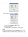
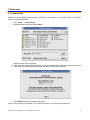
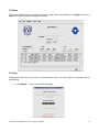
Fast Tester Tool for CCDs v1.0
FTTCCDs
Pamela Hernandez: [email protected]
Alejandro Castañeda: [email protected]
USER MANUAL V1.0
Fast Tester Tool for CCDs
Table of contents
1. Introduction
1.1 Test stand description
1
1
2. Getting started
2
3. Interface description
3.1 Menu bar
3
4
4. Examples
4.1 Example Exposure Run
4.2 Example PTC Run
4.3 Example QE Run
6
6
7
9
5. Extra tools
5.1 Custom script
5.2 Noise
5.2 X-ray
11
11
12
12
6. Acknowledgements
15
7. References
16
1. Introduction
The Fast Tester Tool for CCDs (FTTCCDs) has been developed to help testing the CCDs for DAMIC [1],
DESI and other projects in the test stand at CCD TEST AREA in the SIDET, building at Fermilab[3]. This
interface is programmed in python and uses the Tkinter [4] package to create graphic user interfaces, as
well as the Labview-based application Panview to perform the CCD readout.
This tool integrates several scripts that have been developed by the Fermilab group to acquire and process
CCD images taken with specific test stand.
1.1 Test stand description
The stand composed of the following items:
1.
2.
3.
4.
5.
6.
7.
8.
9.
Monochromator Cornerstone 130
LakeShore 332 temperature controller
Optical Power Meter Oriel
Lamp Oriel
Filter Newport 74040
Shutter Newport 71455
Monsoon CCD readout system
Power supply
IP box
10. X-ray source (Fe55)
11. Cube
12. Collimator
13. Baffel location
14. Linux system
15. Vacuum pump
16. Compressor
17. Photodiode
18. Amperimeter
3
2
4
12
5
1
6
11
13
10
8
7
*The letter in parentheses refer to the tags in section 2
1
2. Getting started
To start the tool, open a terminal (console), get into your kerberos account and connect to decam11. Once
there, go to /home/sispi/CCDtest_tools/interface, and then type: python fttCCD.py, a window will be
displayed.
>> ssh -Y -l sispi decam11.fnal.gov
>>/home/sispi/CCDtest_tools/interface
>> python fttCCD.py
*The letter in parentheses refer to the tags in section 2
2
3. Interface description
The interface looks as show in the following image:
a
Menu bar
b
c
d
f
g
h
e
m
i
j
k
q
l
n
o
p
r
a) Panview Start Button. Click this button to start Panview.
j) PTC Start time spinbox. Start time (in seconds) for Photon
Transfer Curve measurement.
b) Detector Name box. Define a Detector name in order to
organize the folders and files.
k) PTC Stop time spinbox. Stop time (in seconds) for Photon
Transfer Curve measurement.
c) Exposure time spinbox. Use to set the duration of each
exposure in seconds.
l) PTC Step. Increment (in seconds) for Photon transfer curve
measurement.
d)VSUB switch. Click to toggle between on or off the
substrate voltage.
m) QE select box. Select this box to take data for a Quantum
Efficiency curve.
e) Substrate voltage status box.
n) λ1. The lower limit of wavelength (in nanometers) for
Quantum Efficiency curve.
f) Exposure select box. Click on this box to take a simple
exposure.
o) λ2. The upper limit of wavelength (in nanometers) for
Quantum Efficiency curve.
g) Quantity spinbox. Select the number of exposures to
take.
p) Step. Wavelength increment (in nanometers) for Quantum
Efficiency curve.
h) Dark exposure check box. if unchecked, a uniform
illumination exposure will be taken.
q) Message log. Relevant messages of the run status appear
here.
i) PTC select box. Click to take data for a Photon Transfer
Curve (PTC).
r) Apply button. Press when ready to run test.
*The letter in parentheses refer to the tags in section 2
3
3.1 Menu bar
File
Pan open will start Panview (it is same action as “start Panview”), and Pan close this will close Panview
Exit: this option close the interface, also you can close Panview.
Edit
Current offset voltage [volts]: get and set the offset voltage in the CCD. The range of this voltage is [-5,5].
Current integration width: This option can modify the integration width. The default value is 64
nanoseconds.
Analysis
Noise: used to calculate the noise in a exposure.
X – Ray: tool to help to take a X-ray exposure.
*The letter in parentheses refer to the tags in section 2
4
Tools
Custom script: it will run a script previously defined by the user.
Help
About: interface information, and details about authors.
*The letter in parentheses refer to the tags in section 2
5
4. Examples
4.1 Example Exposure Run
Follow this procedure to obtain a CCD read out, here you can take a dark or flat exposure.
1. Press Start Panview button (a*) to run Panview. When Panview is ready, the button will be
disabled and you will see a message in the log . ( Warning: If Labview was running before you opened
the interface, this button will show you a message asking if that process is a Panview process).
2. Specify the name of the detector (b*), (NOTE: This option isn't required for an Exposure run, but it is
recommended to organize the files).
3. Select the exposure time(c*).
4. Select the EXPOSURES selector box (f*).
5. Select the desired number of simple exposures (g*).
6. Select Dark (h*) for a Dark exposure, do not selected for a flat exposure.
7. Press Apply (r*) to set the details selected. A new window will be displayed:
8. Press Go test if the details are correct to start the test.
9. When the process is running, a “In process” window will appear.
*The letter in parentheses refer to the tags in section 2
6
Note: Press abort to cancel test
10. When the test is finished, you will see a message “ [#] Dark/Flat exposure done” in the log (q*), [#]
will be replaced with the number of exposure that you selected in (g*). (Warning: if you ran the FTT
in snowstorm, probably some messages will overlap)
11. The data have been saved in /data/desi/Date_EXDetector$ ($: will be replaced whit a D if you select a
Dark exposure, or F if you select a flat exposure). Examples:
If the detector= DESI-4
Folder: /data/desi/23Jul2014_EXDESI-4
Files: 23Jul2014_EXDESI-4F1483.fits
4.2 Example PTC Run
Follow this procedure to obtain a data to do a Photon transfer curve. This process takes two exposures of
each exposure time, the number of exposures will be taken by
N exp=( stop−start
+1)×2
step
1. Press Start Panview button (a*) to run Panview. When panview is ready, the button will be
disabled and you will see a message in the log. ( Warning: If Labview was running before you opened
the interface, this button will show you a message asking if that process is a panview process).
2. Specify the name of the detector (b*), (NOTE: This option isn't required for a PTC run, but it's
recommended to organize the files).
3. Select the PTC box (i*).
4. Set the desired Start time for the PTC (j*).
5. Set the desired Stop time for the PTC (k*).
6. Set the desired Step for PTC(l*).
*The letter in parentheses refer to the tags in section 2
7
7. Press Apply (r*) to set the details selected. A new window will be displayed:
8. Press Go test if the details are correct to start the test.
9. When the process is running, a “In process” window will appear.
Note: Press abort to cancel test
10. When the test has finished, you will see a message “PTC 100% complete” in the log (q*). (Warning:
if you ran the FTT in snowstorm, probably some messages will overlap)
11. The data have been saved in /data/desi/Date_PTC#_+Detector (#: will be replaced with the test's
number that has been taken). Examples:
If the detector= DESI-4
Folder: /data/desi/23Jul2014_PTC1_DESI-4 Files: 22Jul2014_PTC1_DESI-4_1415.fits
Analysis
To do an analysis you have to run stat.py typing in the terminal: python stat.py, after execute this program,
you will have four files: ptcE1.dat, ptcE2.dat, ptcE3.dat and ptcE4.dat.
You will also need the root macro ptc.C, you can find it in decam11 in: /home/sispi/juan. Save files .dat in a
folder with ptc.C, and run it in root. As a result of running you will get the four pdf which containing the
graphics.
*The letter in parentheses refer to the tags in section 2
8
4.3 Example QE Run
Follow this procedure to obtain data to do a Quantum Efficiency curve, this process take exposures with
different wavelengths. The number of exposures will be taken by
1
N exp= λ2−λ
+1
step
Note: To do a QE test, the user should have a windstorm authorization.
1. Press Start Panview button (a*) to run Panview. When panview is ready, the button will be
disabled and you will see a message in the log. ( Warning: If Labview was running before you opened
the interface, this button will show you a message asking if that process is a panview process).
2. Specify the name of the detector (b*), (NOTE: This option isn't required for a QE run, but it's
recommended to organize the files).
3. Select the QE box (m*).
4. Set the desired λ1 for the QE (n*).
5. Set the desired λ2 for the QE (o*).
6. Set the desired Step for QE(p*).
7. Press Apply (r*) to set the details selected. A new window will be displayed:
8. Press Go test if the details are correct to start the test.
9. When the process is running, a “In process” window will appear.
*The letter in parentheses refer to the tags in section 2
9
Note: Press abort to cancel test
10. When the test has finished, you will see a message “QE 100% complete” in the log (q*). (Warning:
if you ran the FTT in snowstorm, probably some messages will overlap)
11. The data have been saved in /data/desi/Date_QE#_+Detector (#: will be replaced with the test's
number that has been taken). Examples:
If the detector= DESI-4
Folder: /data/desi/23Jul2014_QE1_DESI-4 Files: 23Jul2014_QE1_DESI-4_1893.fits.
*The letter in parentheses refer to the tags in section 2
10
5. Extra tools
5.1 Custom script
Besides the three analysis defined before, the ftt can also execute a user define script. To execute a
custom script do the following:
1. Go to Tools → Custom Script
2. Select the desired script and press Open.
Another window will be displayed
3. If the script required any arguments add it in the box separated by a space as shown in the picture.
4. If the script you selected require Panview, add the root name in the next box.
5. Press RUN and wait to complete the process.
Note: If the script that you selected is not a Panview process, is not required start Panview.
*The letter in parentheses refer to the tags in section 2
11
5.2 Noise
This option calculate the noise in the last exposure saved. To do this analysis go to Analysis and click in
Noise. The Noise information will appear in the log.
5.3 X-ray
Exposing the CCD to an X-ray source is not an automatic process. In order to take an X-ray exposure, do
the following:
1. Go to Analysis → X-ray. A new window will appear.
*The letter in parentheses refer to the tags in section 2
12
2. To position the source , gently turn the knob clockwise until it reaches the stop. Then click in select
box Prepare x-ray Source. See the red message.
3. Press Next to start. The chronometer will start after cleaning the CCD (this an automatic process).
See the red message.
4. Hide the source and click in select box The source is hidden try to do it at the same time in order
to have a more accurate exposure (the exposure time is approximate) , this action will stop the
exposure and the chronometer will stop. See the red message.
5. Press Start Acquisition to begin the readout. See the red message.
*The letter in parentheses refer to the tags in section 2
13
The data will save in /data/desi/Date_XRAY#Detector (#: will be replaced with the test's number that has been
taken). Examples:
If the detector= DESI-4
Folder: /data/desi/23Jul2014_XRAY1DESI-4 Files: 23Jul2014_XRAY1-4_1484.fits
*The letter in parentheses refer to the tags in section 2
14
6. ACKNOWLEDGEMENT
We would like to thank Dr. Juan Carlos D'Olivo and Dr. Juan Estrada because of their expert
guidance and encouragement throughout this work, as well as Dr. Javier Tiffenberg for his support.
We would like to thank to Dr. Alexis Aguilar for his help and his many suggestions.
We acknowledge support from DGAPA-UNAM (PAPIIT) grants No IN112213 and IB100413.
*The letter in parentheses refer to the tags in section 2
15
7. REFERENCES
[1] http://astro.fnal.gov/projects/DarkMatter/DAMIC_project.html
[2]http://physics.lbl.gov/MSDesi2013/cgi-bin/participants.pl
[3]http://www.fnal.gov/
[4]www.nmt.edu/tcc/help/pubs/tkinter/
*The letter in parentheses refer to the tags in section 2
16