Download Population Management 2000 User`s Manual - Training

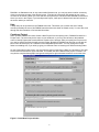
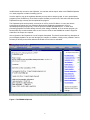
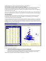
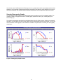
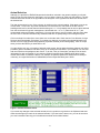
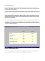
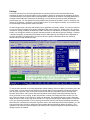
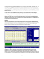
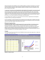
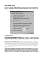
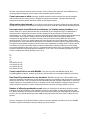
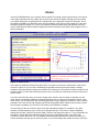
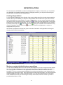
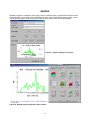
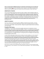
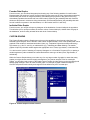
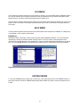
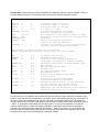
Population Management 2000
User,s Manual
PM2000 version 1.163
14 July 2002
Robert C. Lacy
Chicago Zoological Society
Jonathan D. Ballou
National Zoological Park
Smithsonian Institution
Software developed by:
Jonathan D. Ballou, Robert C. Lacy, and JP Pollak (Cornell University)
Support provided by:
American Zoo and Aquarium Association
The Walt Disney Company Foundation
Chicago Zoological Society
National Zoological Park
Cornell University
Lincoln Park Zoo
Manual citation: Lacy, R.C., and J.D. Ballou. 2002. Population Management 2000 User“s Manual. Chicago
Zoological Society, Brookfield, IL.
Software citation: Pollak, J. P., R. C. Lacy and J. D. Ballou. 2002. Population Management 2000, version
1.163. Chicago Zoological Society, Brookfield, IL.
2000-2002 Chicago Zoological Society
INTRODUCTION TO PM2000
The Population Management 2000 (PM2000) software package provides a suite of tools for genetic and
demographic analysis and management of pedigreed animal populations (a ”studbook‘). PM2000 combines
the capability of the MS-DOS programs GENES (written by Robert Lacy, Chicago Zoological Society),
DEMOG (written by Laurie Bingaman-Lackey and Jon Ballou, National Zoological Park), and CAPACITY
(written by Jon Ballou), as well as adding some new features. PM2000 was developed by JP Pollak (Cornell
University), Bob Lacy, and Jon Ballou. Support for the development of PM2000 was provided by the
American Zoo and Aquarium Association, The Walt Disney Company Foundation, the Chicago Zoological
Society, the National Zoological Park, Cornell University, and the Lincoln Park Zoo. PM2000 is copyrighted,
but it is distributed as freeware for use by anyone who has a need for it. It is illegal for anyone to sell in
whole or in part PM2000 without prior permission from the Chicago Zoological Society.
PM2000 is a Windows program, and it can run on Pentium class computers running Win95, Win98,
Win2000, or WinNT. It requires about 2 MB of disk space for the program files and up to about 7 MB of
space for system files that it may need to load onto the computer. It may not run on computers with 32 MB
RAM, and it will run best if there is at least 64MB of RAM. More memory is needed to analyze very large
studbooks (more than about 4000 animals).
Installation
PM2000 is normally distributed on a CD. To install PM2000, run the SETUP program on the CD. The
installation is available for downloading at http://www2.netcom.com/~pm2000/pm2000.html. Updates of the
program will be posted on this site as well. During installation, it is recommended that newer system files
already on the computer should not be over-written. If Access Violation errors occur during installation, they
can usually be safely Ignored, and the installation will still proceed successfully.
Prior to installing a new version, make sure that no files in the existing pm2000 folder or the Sparks
studbook folder have the read-only property set. After upgrading to a new version of pm2000, create new
projects rather than trying to load any existing projects (see below).
PM2000 may not display well with some Settings of computer screens. If labels of PM2000 run off the edge
of the screen, or the screens otherwise are problematic, you should try alternative Display Settings. These
Settings can be accessed via the Control Panel > Display > Settings. Usually, PM2000 displays well with a
Screen Display Area of 1024x768. A Screen Area of less than 800x600 will often cause problems. Font size
(accessed through the Advanced button of the Display Settings in Win98) seems to work well when it is set
at Large fonts. For some monitors, however, settings other than those described above may be better. The
MS Office menu bar may cover part of the PM2000 display. If that happens, set the Office bar to AutoHide.
Support
Help in using PM2000 can be obtained from the Population Management Manual (Wiese and Willis, in
prep.), and from Help messages, screen prompts, and Wizards built into the program. Members of the AZA
Small Population Management Advisory Group will often be able to provide assistance to users of PM2000.
The staff of the AZA Population Management Center in Chicago can also field questions regarding use of
PM2000. The Population Management Center can be reached at [email protected]. Any reports
of apparent bugs in the software should be sent to [email protected], but the program is provided
without any guarantee that bugs will be fixed. Further development and support of PM2000 will depend on
resources being provided for that purpose.
Starting PM2000
Before running PM2000, files with data on the demographic rates and with data on the pedigree must be
created. The easiest way to create these is to use the SPARKS program, developed by ISIS (International
Species Information System, http://www.isis.org), to manage the studbook data. From the Reports >
2
Analysis > Export menu of SPARKS, you can export the needed files for demographic and genetic analysis.
Sample files (fdefault.prn, mdefault.prn, and default.dbf) are provided in the PM2000 installation.
Care should be taken in determining exactly which data to export from SPARKS. PM2000 will use the
animals defined in the SPARKS View for the Genetic Export as the managed population, although animals
can be removed and added from that View before genetic analyses are run. To use PM2000 with a dataset
that was created outside of SPARKS, see Appendix A.
To start PM2000, double-click on the pm2000.exe program file or short-cut (
). Initially, you must
create a new PM2000 ”Project‘. Your Project will be a set of analyses and reports associated with a data
set. You may create several Projects from a data set (perhaps using different options for the analyses, or
making management recommendations based on different assumptions or goals), and you may create
several Projects from alternative sets of demographic and genetic information from a given studbook. All the
information associated with a Project will be stored in files in a project folder (or directory).
Figure 1. Opening screen of PM2000
PM2000 Wizard Mode
PM2000 can be run in either a Wizard mode or Standard mode. To create a Project in Wizard mode, select
”Let the Wizard Help Me‘ from the opening screen. In Wizard mode, PM2000 will guide you through a logical
sequence for completing analyses and making decisions about managing your population. At each screen,
the Wizard will provide a message box with instructions about what to do at that step. The message screen
shows only about 5 lines of text, but it can be scrolled to show the rest of each message. At the bottom of
each message provided by the PM2000 Wizard, you must either hit –Next“ to proceed with your guided
analysis, hit –Back“ to return to the previous Wizard page, hit –Exit Wizard“ to end the Wizard and use
3
PM2000 in its Standard mode. At any screen within Wizard mode, you can jump back to earlier screens by
clicking on the page number of the desired screen. (The label of each screen will appear as your cursor
moves over its number.) When you close and save a Project that is in Wizard mode, PM2000 will remember
where you were in the Project. If you later Open the Project, it will open in Wizard mode and will resume at
the screen where you last left it.
Help
A Help utility can be opened from the PM2000 menu bar. This allows you to search the text of a Help
manual (essentially the text of this PM2000 manual and the text shown in Wizard mode). You can also scroll
through the documentation to find needed information.
Creating a Project
When you start PM2000 and select Create a New Project from the opening menu, PM2000 first asks for a
Project name. The name may be the same as your studbook, or you may use variants on the studbook
name to identify Projects that contain different versions of the analysis. After you specify the Project name,
you need to specify the folder that will store the Project. By default, PM2000 sets the folder to one with the
same name as the Project, as a subfolder of the \PM2000\Projects folder. You may change the Project
folder to something else, if you wish, by typing in a different name or browsing to a different existing folder.
On the Create New Project screen, you also have the option of specifying a Date for Calculations. This date
will be used to determine the ages of animals. The default date is the date that the project is created. You
may wish to complete demographic and genetic analyses for ages calculated relative to some other date.
Figure 2. Create New Project window
4
Next, you must specify the names and locations of the files with demographic information on females and
males. By default, PM2000 will look for files named the \sparks\project\fproject.prn and
\sparks\project\mproject.prn, with ”project‘ replaced by the name of your project. If the files do not exist with
these names, or if you wish to use other demographic data files, you specify those files by typing in the
filenames or browsing to find the files.
If you have not previously prepared .prn files with demographic information, you can specify that no
demographic data will be imported into your Project. PM2000 will then use default demographic data. Within
Demography analyses, you can then modify these defaults to test the effects of other demographic rates.
A genetic information file is specified next. PM2000 will first look for a file named \sparks\project\project.ped
or \sparks\project\exchange.dbf. If these are not found, or you wish to use a different file, you would specify
that file. The project.ped file is a file created by PM2000 when you first create a Project. It is a text file
version of the information in the exchange.dbf file. By saving the pedigree information in the .ped file,
PM2000 allows you to later retrieve the pedigree data on which a Project was originally based (perhaps for
creating a new Project from the same genetic data), even if you have overwritten the exchange.dbf file
created by SPARKS. You can specify that no genetic information will be imported into your Project. In that
case, when you begin genetic analyses you will need to type in the animals and their parentage for your
population.
It should be noted that the ”genetic information‘ file will be used for more than just obtaining the parentage
data for genetic analyses. This file also provides data as to which animals are in the selected subset of the
population that will be the focus of management. Thus, not only genetic analyses, but also age structure and
the starting population for population projections will be based on this managed subset of the population.
(The .prn files with demographic information will be used only to provide the mortality and fecundity rates for
demographic analysis.) Therefore, in creating the ”genetic information‘ file from SPARKS or otherwise, it is
very important to pay close attention to which animals are selected for analysis.
After specifying the files with input data, you can add any notes to a Comments section of the Create New
Project screen. These comments will be automatically transferred to your Clipboard report. It would be
useful to use these notes as an opportunity to document any assumptions you made or other special
considerations about the data that you imported into your Project.
When working on a PM2000 Project, you can move among six sections of the program: the PM2000
Clipboard, Demography, Genetics, Goals, MateRx, and Metapopulations. PM2000 can also create a set of
pre-formatted reports for the breeding and transfer recommendations of population management, it provides
a variety of graphs, and it contains Help and a dictionary with Definitions of genetic and demographic terms.
YOUR PM2000 CLIPBOARD
After you have entered all the information needed to create your Project, you click on the Create button and
PM2000 takes you to the Clipboard (a report editor). Automatically transferred to the Clipboard will be
documentation of the Project name and date, the files used for demographic and genetic information, and
any text describing the data view used when the data were exported from SPARKS. The Clipboard provides
you with basic text editing tools, for cutting and pasting, or adding and deleting text. To edit, you can use
standard Windows short-cut keys, or select actions from the Report Menu.
On the Clipboard, you will accumulate text, tables, and graphs that document your analyses and
management decisions. It is a good idea to send information liberally to the Clipboard as you work in
PM2000, and then later to go back to edit and delete unnecessary information. On each screen in PM2000,
and for some subsections of screens, there is a –Send-to-Report“ icon ( ). Clicking on that icon will send the
associated text, tables, and/or graphs to your Clipboard. Often-times, formatting of tables and text is
5
modified when they are sent to the Clipboard. You can later edit the report, either in the PM2000 Clipboard
or in other programs, to obtain formatting you like.
It is also useful to copy to the clipboard data that you may wish to analyze, graph, or use in spread-sheet
programs (Excel, PowerPoint). First –Send-to-report“ the data you wish to use, then select the data from the
Clipboard and copy it directly into the spread-sheet program.
The Clipboard report can be printed, or saved as an .rtf file, via the File Menu. You can also retrieve
previously saved reports into your Clipboard. Because the Clipboard is saved as an .rtf file (in
\pm2000\projects\project\project.rtf), it can be opened in WORD, WORDPERFECT, or other word
processing programs for further editing. However, after editing a PM2000 .rtf file in another program, you
should either save it under another name or save it as an .rtf file so that PM2000 can read the original or
edited file if the Project is re-opened.
At the right side of the Clipboard is a list of Analyses Completed. This list will accumulate key descriptors of
your managed population as you work through your analyses. In addition, clicking on any variable in the list
will take you directly to the screen where that variable can be found or calculated.
Figure 3. The PM2000 Clipboard
6
DEMOGRAPHIC ANALYSES
When you created your Project, PM2000 read in demographic data from .prn files and performed a number
of analyses. You click on the Demography heading to begin your demographic analyses. The following
sections describe each tabbed page available within Demography.
Male and Female Life Tables
The life-tables for males and females are created from the data exported from SPARKS. The Life Table
screens show the average survival and reproductive rates for males over the time period you selected when
exporting the data from SPARKS. PM2000 also calculates the population growth rate (lambda and r) for a
stable population under these conditions as well as generation length (T), current number of males (N) and
projected number of males twenty years from now (N20). (Note that unknown sex animals are counted as
50% male, 50% female so you may have fractional males). Also shown are the sample sizes (# animals at
risk) used to calculate the Mx and Px values, life-expectancy (Ex) and reproductive value (Vx).
On the left side of the Life Table screen is the ACTUAL life-table. These are the data exported from
SPARKS. On the right is the MODEL life-table. The Mx (fecundity) and Px (Survival) rates on the screen are
initially the same as the ACTUAL screen. However, the you can use the MODEL screen to smooth the to
data by clicking the text below the table. You can also change the Px and Mx values in the MODEL life-table
but not in the ACTUAL table.
Figure 4. Life Table screen
At this screen, you should first check that the smoothing of the Mx and PX is reasonable. The object is to
derive a Mx and Px curve (and hence Lx curve) that reflects the characteristics of the population to the best
of your knowledge. Poor data quality and quantity are a problem in many studbooks. Smoothing the data
can help to provide more reasonable estimates of life-table rates. However, smoothing can sometimes lead
to unreasonable values. You need to check the life table for any smoothing problems and modify the
smoothed Px or Mx values if this is the case. So check the following:
7
Is there reproduction in pre or post reproductive ages? If so, zero these out.
Check the graphs of Actual vs. Model Mx and Actual vs MODEL Px.
Use knowledge of the species“ biology, husbandry and management to modify the Mx values as needed.
Modifications that significantly change lambda or generation length should be evaluated carefully.
You can reset the values to original values imported from SPARKS by selecting the Data > Demography >
Reset option on the menu bar.
Once you are happy with the life table, or can explain away all its peculiarities, copy it to the Clipboard. You
may want to cut and paste the life-table from the Clipboard to a spreadsheet program to enhance graphics.
Age Distribution
The Age Distribution screen shows the number males (left) and females (right) in different age classes.
Each bar is a one-year age class. Under the age distribution is the total number of male, female and
unknown aged animals currently in the population.
The table shows the actual numbers, and the numbers expected for a stable age distribution. A stable age
distribution is the number of animals in each age class that we would expect if the life table rates had been
constant over time. You can change the numbers of animals in different age classes. Unknown sex animals
are assigned to be 0.5 male and 0.5 female.
Figure 5. Age Distribution screen
Take a look at the age distribution:
Are there any impossibly old animals? (if so, check your SPARKS data).
Does the age structure show a baby boom or is it top or bottom heavy?
Are there enough animals in breeding age classes to provide the desired amount of reproduction?
How does the actual age distribution compare to the stable age distribution? If they are quite
different, then population growth may behave unpredictably in the future.
8
Male and Female Projections
The Projections screens show the expected number of males or females in the future given the model lifetable and the actual age distribution. The projected numbers if the age structure was stable are also shown.
The difference between the actual and stable projections shows the impact of the age distribution. For
example, a population with fewer breeders than expected (if the population were stable) might actually
decrease in size in the near future as a result even though the life-table predicts a positive growth rate
(lambda > 1.0).
Total Projections
On the Total Projections screen, the projections for males and females are combined.
Figure 6. Projections screen
9
Reproductive Planning
Use the Reproductive Planning screen to determine how many births (or culls) you need to get to your
desired or target population size. In the upper left corner of this screen, you specify the target size and the
desired rate (or amount of time) to reach that target. If you need to increase population size, PM2000 will
use the population growth rate from the demographic analyses to determine how fast you can grow the
population (and thus how long it will take you to get to your target size).
The numbers in the table at the upper right show you how many births you need this year, next year, the
year after, etc, to get to and maintain the population at the target size. The Model life tables you set up
earlier are used to make these calculations. These calculations take into consideration the neonatal
mortality rates so the table really does show the number of births needed as opposed to the number of
surviving births. You can change any of the values to explore various options.
If you need to decrease the population size, the table may show negative numbers. These are the number
of animals you must remove from the population to cause the population to decline to the target size.
Figure 7. Reproductive Planning screen
To simply maintain population size (a zero-population growth management plan) all you will need to do is
produce enough births to balance the death rate. Set the target size at the current size and lambda will
change to 1.0. The number of births needed to replace expected deaths will be shown in the table.
Once you have the number of births needed, you need to determine how many breeding pairs or groups you
need to set up to produce these numbers of births. Use your experience and knowledge of the biology,
husbandry, and behavior as well as your knowledge of the individuals in the population to specify in the
lower left part of the screen the expected mean litter or clutch size and the probability that a pair will breed.
PM2000 will apply these numbers to its calculation of the number of births needed, in order to determine for
you how many pairs you should put together for breeding.
10
At the lower right of the Reproductive Planning screen is a graph that shows the projected growth and then
stability of your population, assuming that all goes according to the plans you have specified. If you check
the box at the bottom left, PM2000 will then transfer this projection to the Population Projection screens.
Standard Demography Graphs
The last tabbed screen available in the Demography section provides a set of four standard graphs. The
graphs provided are age-specific rates of fecundity (Mx), reproductive value (Vx), mortality (Qx), and
survivorship (Lx).
The data for these graphs are taken from the Model Data in the Life Table screens. Unless you smoothed
the data in your life tables, the lines on the graphs may be rather jagged and hard to interpret. You can use
the smoothness of these graphs as an indication of whether it may be useful to smooth your demography
data further.
Figure 8. Demography Graphs screen
11
GENETIC ANALYSES
Getting Started with genetics
When you created your PM2000 project, you specified a file to be used for gathering genetic information.
This file was either a .dbf file or a .ped file. Most users will export a file for genetic analysis from the
SPARKS studbook software. SPARKS automatically names this file exchange.dbf. Alternatively, you may
have created your own .dbf file containing a pedigree for analysis with PM2000 (see Appendix A).
After the first time that you use exchange.dbf (or another .dbf file) for sending genetic information to
PM2000, PM2000 will create a text file, called project.ped (with ”project‘ replaced by the name of your
project) that contains the pedigree information from the .dbf file. The advantage of this file is that it is saved
with a name that associates it with your project, and it can be used again in the future if you need again to
read the genetic information into your PM2000 project. Therefore, if you subsequently export more genetic
information from SPARKS, SPARKS will over-write your exchange.dbf file, but you will still have a saved
copy (under the name of project.ped) of the pedigree information that was used in your PM2000 project.
If you ever need to restore the pedigree information in your PM2000 project back to the pedigree that was
first read in, you can do so by going to Data > Genetics > Reset on the menu. If you wish to replace your
pedigree information with data from a different pedigree information file, you can do so by going to Data >
Genetics > NewData on the menu.
Before beginning your genetic analyses, you might note that the Clipboard automatically contains a line that
specifies what file was used for genetic information, and ”Additional genetic information‘ specifies what View
criteria were used when the genetic data were exported from SPARKS. You might add any further notes to
the growing report on your Clipboard, as necessary or useful to document the genetic analyses that you are
conducting. (A warning: It is extremely hard to remember, when you look back at a project months after it
was first created, why certain animals were included or not in your analysis, and why you made other
particular decisions about the population analysis and management. USE YOUR CLIPBOARD to document
your analyses.)
You click on the Genetics heading to begin your genetic analyses. The following sections describe each
tabbed screen available within Genetics.
12
Animal Selection
Although you specified in SPARKS what animals should be included in the genetic analysis (you did this
when you set the View Criteria for the Export), you now have a chance to "touch-up" this selection. The lefthand list shows the animals in the population to be analyzed. In the right-hand list are those animals not in
the selected set.
The lists can be sorted on any of the columns, by clicking on the column heading. Click again to sort in the
reverse order. To find out if any sterile animals are in the selected set, click twice on the Sex column
heading and check for animals that are listed as being sex = –s“. You probably want to remove these animals
from the set selected for genetic management. Animals with sex = –m“ or –f“ (rather than –M“ or –F“) are
contracepted males and females, respectively. You may then want to sort on location, and then scan down
the list to see if it includes animals at any institutions that are not participating in the management plan.
Click on animals from either list to move them over to the other side. Check the box ”Use Selection for Age
Structure and Demographic Projections‘ if you want any changes you make in the selected animals to be
carried over to the age pyramid and population projections screens (under Demography). Click on Accept
when you have the lists as you want them to be.
You can edit the sex, age, or location of animals at this screen, but be aware that these changes only affect
pm2000“s genetic calculations and tables; they do not change the data back in your studbook. You can also
add new animals to the pedigree at this screen. To do this, click on Create New, and then fill in the basic
information for each new animal. If you leave any fields (except ID) blank, PM2000 will fill them in with
default values when it creates the animal. For example, unspecified parents are assumed to be UNK (for
unknown), an unspecified location is UNKNOWN, and an unspecified birth year is 2000.
Figure 9. Animal Selection screen
If you made any changes to the selected animals, this is a good time to go back to the Clipboard and write
down what changes you made in the selected animals. If you don't write it down now, you can be sure that
you won't remember later why you included some animals and excluded others!
13
Population Statistics
After you accept your Animal Selection, PM2000 proceeds with the genetic analyses. When it is done, it
takes you to the Population Statistics screen. This screen displays the basic summary statistics describing
the genetic health of your population.
Take time to look at how many founders have contributed to your captive-born population, how much gene
diversity there is in the captive population relative to the wild population from which the founders came, the
number of founder genome equivalents (how many wild-caught animals would have the same gene diversity
as the captive-born population), and the mean inbreeding level of the population. Take time also to look at
what these values could become (the "Potential") if you could perfectly control all breeding, production of
offspring, and which genes are transmitted to offspring. (Unless you bring in new founders, you can never
reach this theoretical ”potential‘, rather it is an upper limit that gives you an indication of how much scope
there might be for improvement.)
The number of Living Descendants may be less than you expected, and may even be a fractional number.
This is because PM2000 normally excludes all animals with unknown parents from genetic analyses, and
includes only those parts of animals which can be traced back to known founders. For example, an animal
with a known dam but an unknown sire will be tallied as half an animal in genetic analyses. As will be
explained later, you can change the way that PM2000 handles unknown parentage by going to the Settings
> Genetics > General Options menu.
Figure 10. Population Statistics screen
At the bottom of the screen you will notice that there are listed a few of the more useful measures of the
genetic status of the population. This footnote will be displayed on each of the Genetics screens, and the
values may change as you make recommendations for breedings and/or cullings.
14
Founder Statistics
This screen shows a list of all founders and some statistics about their genetic contributions to the living
captive-born population. On this screen, as in most tables in PM2000, you can sort the list on any of the
listed measures by clicking on that column heading. If you click on a column heading for a second time, the
list will be sorted in descending order. Sort the founder list by the Living/Dead column, in order to see if
there are any living founders. If there are, you might take note of them now. Living founders should probably
be given preference in breeding over non-founders that have similar (or larger) mean kinships.
Figure 11. Founder Statistics screen
If you specify that UNKnown animals are to be treated as WILD (see Genetic Options, below), then the
founders that have UNK parents will be indicated with a –U“ after the studbook #.
You may see some founders with studbook numbers of Pxxx (in which xxx is another animal“s studbook
number). These are ”pseudo‘ animals that had to be created by PM2000 to complete the pedigree. These
animals are the UNKnown parents of animals whose other parent is the xxx animal. Thus, if an animal has
dam –123“ but an unknown sire, the sire –P123“ would be created and given parents UNK. An exception to
this occurs if the dam is herself wild-caught. In that case, it is assumed that the dam was pregnant wen
captured, and the sire –P123“ is given parents WILD.
15
Individual Statistics
The screen at this next tab lists all the living animals in the selected population, along with some basic
information (parentage, age, etc.) and various measures of current genetic value to the breeding program.
You can get more information about the various genetic measures reported by PM2000 by reading the
Population Management Manual. If any values in the table are é1.000, this means that the number could not
be calculated or was not applicable. (For example, founders do not get a value for the GU-Desc, the
Genome Uniqueness among descendants, not counting the founders).
Figure 12. Individual Statistics screen
Inbreeding
The Inbreeding tab displays a list of the inbreeding coefficients (symbolized by 'F') of the analyzed
population. You can use this list to assess whether more inbred animals have shorter life spans (if you
Selected Living and Dead animals when you exported the genetic data from SPARKS), or you can ignore
this screen and go on to more interesting parts of the genetic analysis. Brackets around an ID indicates that
the animal is dead; the age given for a dead animal is the age at which it died.
Kinship Matrix
The kinship coefficients between every pair of animals in the population are displayed in a table accessed
by the Kinship Matrix tab. Most of the numbers shown in the genetic analyses can be calculated from the
table of kinships. (For very large studbooks, the kinship table is not shown, as it is too large to be easily
viewed. However, it will always be stored as a file named project.kin in your Project folder, so you can view it
later if you wish.) If you want to find the kinship between any two animals, click on the option below the
table. The kinship between two animals is also the inbreeding coefficient of any offspring produced by
mating the two animals. Thus, this option allows you to examine whether a potential mating would produce
inbred progeny.
16
Pairings
This screen allows you to select the optimal pairs of animals to breed, and to test what effect those
breedings will have on the genetic status of your population. When you select pairs for breeding, the effect
of those breedings on the genetic status of the population depends on the number of offspring produced by
each pair. Before starting to select pairs for breeding, you may need to specify how many offspring are
produced per pair. You can specify how many offspring are produced in each litter, clutch, or brood for your
species in the Settings > Genetics > General Options menu. If you change this number, you must then click
on the message to reset genetics options and data.
On the Pairings screen, all males and females in your population are listed in tables. You can sort either list
by any one of several measures of genetic importance: MK, mean kinship; KV, kinship value; GU, genome
uniqueness; P[lost], probability of allele loss; FOKE, first-order kin equivalents; or Rel MK, the relative mean
kinship. You change the measure of genetic importance shown on the table by going to Settings > Genetics
> Weigh Pairings By, and checking the desired measure. Although only one measure will be displayed on
the list of animals for possible pairing, you can see all of the genetic information about any animal by
double-clicking on that animal on the list.
Figure 13. Pairing screen
To sort the list of animals, click on the appropriate column heading. Click on it again if you want to sort in the
reverse order. You can then test the effects on the genetic status of the population of producing offspring
from any pair of animals. Click on the male and the female that you may want to pair to see how Gene
Diversity, Gene Value, and Founder Genome Equivalents would change if that pair produced offspring.
Once you decide to use a pairing, hit the Accept button. Instead of choosing Pairs from the lists, you can
also –Type in a Pairing of your Choice“ by clicking on that label. This option allows you to type in pairs that
might be hard to find in a very long list of animals. You may also test pairings of dead animals or of animals
not in your selected population, if you previously chose those options under Genetics Settings (see below).
After each pair is selected, the measures of genetic value of the remaining animals will be updated. (I.e., the
new parents and any of their kin will become less valuable than they had been before the pairing.) This
updating is not done if the Genetics Option (see below) is set to specify that genetic measures should not
change as pairs are created.
17
Any animals used in pairings will be highlighted in red. If you change your mind after you Accept a pair, you
can ”un-pair‘ it by highlighting it on the list of pairs and then hitting the Remove button. If you want to start
over with selecting pairs, hit the Reset button. As you pair animals, you will see that the summary statistics
of the population will be updated at the bottom of the screen. When you are done selecting pairs, you should
send your list of pairs to your PM Clipboard. Also send to the Clipboard the new Population Statistics at the
bottom of the screen.
You can specify that the hypothetical offspring produced by your pairs should be included in the Age
Structure and Population Projection screens, by checking the indicated box. You can also specify that these
new offspring are to be included in any data file produced for MateRx (see below).
When you exit PM2000, your selected Pairs will be printed to a file called project.prs. You can later ask
PM2000 to add these pairs (or any pairs that have been listed in a .prs file) to any Project by choosing to
Import Pairs from a File on the screen. (The pairs you have chosen will automatically be reloaded with your
Project when you later Open the Project.)
Culling
The Culling screen allows you to identify which animals should be removed from the managed population,
and to test what effect those cullings will have on the genetic status of your population. Any animals that
were already known to be outside of the managed population, or are incapable of breeding, should probably
have been removed already back at the Animal Selection screen, before you began Genetic analyses.
However, at this point you can remove more such animals by culling them here.
Figure 14. Culling screen
In addition, you may use this screen to identify additional animals that should be removed from the
population in order to further the genetic management. If there is limited space available to maintain
animals, you may want to remove genetically redundant animals (sometimes called ”surplus‘) to make room
for production of new and more valuable animals. Sometimes you need to identify some animals that can be
18
safely removed from your population for use in release programs or for export. At this screen, you can sort
the list of animals by any one of several measures of genetic importance: MK, mean kinship; KV, kinship
value; GU, genome uniqueness; P[lost], probability of allele loss; FOKE, first-order kin equivalents; or Rel
MK, the relative mean kinship.
To sort the list of animals, click on the appropriate column heading. Click on it again if you want to sort in the
reverse order. You can then test the effects on the genetic status of the population of removing any animal.
Click on an animal that you may want to remove to see how Gene Diversity, Gene Value, and Founder
Genome Equivalents would change if that animal were culled. Once you decide to cull an animal, hit the
Accept button. After each animal is removed, the measures of genetic value of the remaining animals will be
updated. (I.e., kin of the culled animal will become more valuable than they had been before the culling.) If
you want to ”un-cull‘ all the animals you had selected, hit the Reset button.
You can specify that the animals to be culled should be removed from the Age Structure and Population
Projection screens, by checking the indicated box.
As you cull animals, you will see that the summary statistics of the population will be updated at the bottom
of the screen. When you are done with culling, you should Send to the Clipboard your list of culled animals,
and the new Population Statistics at the bottom of the screen.
Effective Population Size
The effective population size (Ne) is based on the past history of the population, but its primary use is in
predicting future genetic changes. The first estimate of Ne is based on the amount of gene diversity lost
through the generations of captive breeding. This estimate will represent an average Ne over those
generations. The second estimate of Ne is based simply on the number of living males and living females
that have produced offspring. This estimate will reflect the current Ne, but often it will overestimate Ne
because some of the animals that have bred may no longer be breeders or may breed only poorly. Click on
the Send-to-Clipboard icon to record these estimates in your report.
Census
If you ran a Census Report within Sparks, then PM2000 will fetch those data and display them in a table and
in a graph on the Census screen.
Figure 15. Census screen
19
GENETICS OPTIONS
In the Settings > Genetics > General Options menu, you can change some of the assumptions made by
PM2000 for genetic analyses. Unless you are have special analysis needs, and you are very familiar with
how the genetic analyses are calculated, you should probably not change any of these settings other than
perhaps the number of offspring to be produced per pair.
Figure 16. Genetics General Options window
The available settings are:
Include founders in all genetic analyses: Normally, the wild-caught or imported founders are not
included in tallies of the genetic status (GD, GV, and FGE) of your population. Instead, the measures show
the genetic status of the descendant animals produced within your captive population. If you wish to include
the founders themselves in the tallies of genetic status, check this option.
Allow pairing non-selected animals: Non-selected animals are not included in measures of
genetic status (that is why they were not selected), but you may test them in Pairings if you check this box
so that PM2000 will keep information about them in its database. For example, you might wish to test the
effect of importing an animal not presently in your population to use in future pairings. If you check the
option to allow pairing non-selected animals, the genetic calculations will be slower, but you will be able to
use non-selected animals in pairs.
Do not update genetic measures as pairs are created: Normally, PM2000 adds hypothetical
offspring to the population as you create pairings, and updates the measures of genetic value (e.g., Mean
Kinship, Kinship Value) to reflect the contribution of these new animals. This will cause the paired animals
and their relatives to decline in genetic value. However, if pairs to be tested have only a low probability of
successfully breeding, it may be more realistic not to assume that they will add offspring to the population. In
20
this case, they and their relatives would not drop in value. Checking this option will cause PM2000 to not
create hypothetical offspring of chosen pairs, and not update genetic measures.
Count unknowns as wilds: Normally, pm2000 excludes unknown animals from genetic analyses,
and considers only the known portion of pedigrees of partly known animals. This option specifies that
animals with unknown parents should be treated as wild-caught founders.
Allow pairing dead animals: If you wish to test the effects of producing offspring from dead animals
(perhaps from cryopreserved gametes or embryos), you need to check this option before selecting the pairs.
Use input matrix of coefficients of relatedness (or kinship) among founders: These
options allow you to specify that founders are not unrelated (as is usually assumed), but instead have a
specified matrix of relatedness or kinship. Founder kinships could arise because of known familial
relationships (e.g., a litter of siblings), or because molecular genetic evidence indicates close kinship among
some founders. If this option is chosen, there must be in the project folder a file called related.txt or
kinships.txt (as appropriate for the option selected). The file must be an ASCII (DOS text) file, with the
following format. First line is a number stating how many founders are in the relationship or kinship matrix.
(Any founders not in the matrix will be assumed to be unrelated to all other founders.) Subsequent lines give
(one per line) the studbook numbers for each founder in the relationship or kinship matrix. Following the list
of founders, the matrix is specified. Each line lists the relationship or kinship coefficients to each founder,
with a space separating each value. The full, symmetrical matrix must be given. For example, the following
kinship file information would indicate that founders 23, 35, 67, and 101 are full-siblings (kinships of 0.25),
but are not themselves inbred (kinships to self = 0.5).
4
23
35
67
101
0.50 0.25 0.25 0.25
0.25 0.50 0.25 0.25
0.25 0.25 0.50 0.25
0.25 0.25 0.25 0.50
Create output file for use with MateRx: This option specifies that PM2000 should, after
completing genetic analyses, create a file of genetic data for later use in the program MateRx (see below).
Run Gene Drop simulation for nnn iterations: PM2000 normally uses 1,000 iterations of the
gene drop simulation to estimate the genetic diversity remaining in a population and the genome uniqueness
values for each animal. This is enough to provide reasonable precision (usually to better than 1% accuracy),
without requiring an unreasonable amount of computer time for most studbooks. Analyses will be faster if a
smaller number of iterations is chosen. Analyses will be more accurate if a larger number is chosen.
Number of offspring produced per pair: When you select pairs for breeding, the effect of those
breedings on the genetic status of the population depends on the number of offspring produced by each
pair. Before starting to select pairs for breeding, you may need to specify how many offspring are produced
per pair. Here you should specify how many offspring are produced in each litter, clutch, or brood for your
species.
After you change any of the General Options under the Genetics Settings, and then click on OK, PM2000
will redo the genetic calculations using the settings you have selected.
21
GOALS
This part of PM2000 allows you to explore various options for meeting a specific genetic goal. First, specify
in the upper right hand corner a genetic goal in terms of the amount of genetic diversity you wish to retain
over a given time period. A typical goal is to maintain 90% of the wild gene diversity for 100 years. This is
the default in PM2000. (An alternative goal, currently disabled, is the goal to retain at least X% of the gene
diversity throughout a period of Y Years.) The program will start by determining what population size you
need to meet this goal. Notice that the program has retrieved data from other parts of the program to use in
these calculations.
Figure 17. Goals screen
At the start, the ”Maximum Allowed Population Size‘ is set at the current size. At the bottom of the screen,
next to the ”Solve for‘ you can see if maintaining the population at the current size under the existing
conditions (Ne and generation length) can maintain your desired goal. The answer will either be that you can
with this number (or even fewer animals) or that you can“t, in which case it will show you how much you can
hope to retain.
If you can“t meet this goal, then you need to change some values to see how large a population you will
need. Start by increasing the Maximum Allowed Population Size to a larger but reasonable number. If this
doesn“t work, you can experiment with increasing generation length, population growth rate, and/or effective
population size. Play around with changing values (but keeping them within reason) until you have a sense
for how large a population you will need, or how many new founders are needed.
It may be that you still can“t meet the goals even with reasonable changes. For example, if your gene
diversity is already below the goal, no amount of changes will help. In this case it is worth considering
adding new founders. Find the line labeled ”New Founders‘ and change the value to 1. This will activate the
lines below. Set the Maximum Allowed Population size and a reasonable number, and select ”New
Founders‘ from the ”Solve For‘ list. The program will automatically calculate the number of founders you
need to add within the next year to meet your goals. You can also change the number of times or years you
22
hope to add new founders, as well as the frequency. Again, play around with these options until you have an
understanding of how adding new founders will help you achieve your genetic goals.
If you still find that adding founders is impossible (or an unreasonable number are needed) then consider
changing your goal. For very small populations, with no hope of adding new founders, it may only be
possible to maintain 87% of gene diversity for 100 years. The goal can be changed by decreasing the
amount of gene diversity to retain, shortening the time period, or both. For some populations, it might even
be reasonable to set the genetic goals higher than the 90% for 100 years. A large, well managed population
with long generation length and with the option of periodically adding new founders may be able to retain
95% gene diversity for 200 years.
Don“t forget to send to the Clipboard ( ) various scenarios you want to present in your final report.
Finally, set the screen to the scenario you accept as the most reasonable way to meet your goal (number of
new founders, if appropriate, desired population size, any changes in lambda or Ne or T required). The
target population size for the last scenario tested will carry over to other parts of the program (e.g.,
Clipboard“s Analyses Completed, Reproductive Planning) as your goal for population size.
Multiple comparisons
Sometimes it is useful to explore how a range of values in a parameter or pair of parameters affects the
goal. The Multiple Comparisons option (available through clicking on the –Multiple Comparison“ text) allows
you to simultaneously select a range of values for two parameters and create a table of results. So for
example, if you were interested in determining how changes in Generation Length and changes in lambda
might affect the target population size, select –Generation Length“ on the top of the table to set the columns
to different values and select –Max. Potential Lambda“ to set the rows at different lambda values. Usually,
PM2000 will set the middle value as the currently defined value for a parameter, however, these values can
be changed by clicking on the cell. The table will fill with the target sizes needed for every combination of T
and lambda. These results can also be sent to the clipboard.
Figure 18. Multiple Comparisons screen
23
MateRx
PM2000 is designed to export data to an independent DOS-based program called MateRx (Ballou,
Earnhardt, and Thompson, 2000). MateRx is a program that uses a new rating system being developed by
SPMAG to calculate an index which indicates how good (or bad) any pair in a population is relative to
several measures of genetic importance. The MateRx software is designed and developed to be a genetic
tool that will guide population management decisions. For every male/female pair in the population, MateRx
calculates a single numeric index indicating the relative genetic benefit or detriment to the population of
breeding that particular pair. This index, the mate suitability index (or MSI), is calculated from considering
the pairs' mean kinship values, the difference in the male and females mean kinship, the inbreeding
coefficient of the offspring produced, and the amount of unknown ancestry in the pair. MateRx is designed to
simplify the decisions about which pairs should be bred by condensing all that we know about the genetics
of a pair into a single number.
The program can be used to produce a table showing the MSI values for all male/female pairings (which
then can be accessed through word-processing software and printed and distributed) or can be used
interactively to search for specific mates as needed.
MSI values are labeled as beneficial (scores = 1, 2, or 3) or detrimental (scores = 4, 5, or 6) to the
population. Beneficial MSIs denote no detrimental effects relative to the genetic values of that pair, and MSI
values of 4, 5, or 6 indicate at least one detrimental effect.
MSI Score Definitions:
1 = very beneficial pair
2 = moderately beneficial pair;
3 = slightly beneficial pair;
4 = slightly detrimental pair;
5 = detrimental pair, should only be used if demographically necessary;
6 = very detrimental pair, (should only be used if demographic considerations override preservation of
genetic diversity per se).
”-” = so detrimental the pair should never be made.
Because the MateRx process is automated, the software is limited in several ways:
MateRx does not address demographics, behavior, or logistics of a pairing;
MateRx is not intended for use with all captive managed species. Many species have unusual population
histories and structures that require the expertise and attention of a trained population biologist. These
populations may have characteristics such as few founders, many captive generations, extremely small
numbers, or many unknown origins or parentage data that prohibit generic management (see MateRx
documentation for more details).
MateRx is time sensitive: the MSI rankings are only valid as long as there are no substantial changes in the
population. This report should be considered invalid after one year following its date of creation.
The MateRx program file (MATERX.EXE) needs to be loaded into your ”Project‘ folder. The program is
currently set up to assume that your projects are each in a separate folder within the ”Projects folder‘. While
running PM2000, at any time (after the initial Genetics tab is opened) you can click on the MateRx tab to
create or re-create a dataset to run the MateRx program. This dataset will incorporate any removals, new
pairings, or culls that you have imposed on the population. MateRx will run in a DOS window at the same
time as PM2000 and thus can serve as an additional tool for use in developing a population management
plan. See the MateRx documentation for details on running MateRx.
24
METAPOPULATIONS
The last component of PM2000 is a section on Metapopulation analyses. In this section, you can partition
your population into subsets (including nested or overlapping subsets, if you wish) and look at the gene
diversity within and between these subpopulations.
Creating subpopulations
For the population highlighted on the left side of the screen (initially this will be the total project population,
as that is the only one available), the animals in that population will be listed on the right. This list can be
sorted by clicking on a column heading. To create a subpopulation, use your mouse to select the animals
you wish to include, and then click on the subset icon ( ) to create your new subpopulation. The program
will prompt you to name the subpopulation. You can very quickly create a subpopulation for each Location
by clicking on the map icon ( ). The information icon ( ) gives you a snapshot of information about any
animal you highlight, while the delete icon ( ) removes an animal from a population, or removes a
subpopulation from your list.
With the list of populations on the left are given the number of animals in each population and the gene
diversity present within that population.
Figure 19. Metapopulations screen
Moving or copying individuals between populations
You can use the Metapopulation screen to test what would happen if you were to copy or move an animal
from one population to another. (A ”move‘ puts the animal in the new population and removes it from the
old. A ”copy‘ puts the animal into the new population, but still leaves it also as a member of the old
population.) To move or copy an animal, highlight its current (source) population on the left-hand list, then
right-click on the animal on the right. Then drag the animal to the recipient population. You will be prompted
to specify whether you wish to Copy or Move the animal, or to Test one of these actions. If you test the
action, PM2000 will first tell you what new gene diversity would result, and then it will ask if you wish to
proceed with the Move or Copy.
25
Metapopulation comparisons
Clicking on the comparisons icon ( ) will open a screen for making population comparisons. On this screen,
you highlight the populations you want included in the comparisons, and the program will display a table of
all pairwise between-population comparisons. Below the diagonal on this table is the genetic divergence
between each pair of populations as measured by an Fst value. (Fst is a measure of what proportion of the
total gene diversity of the two populations is present as between-population divergence rather than withinpopulation diversity.) Above the diagonal are the between population differences as measured by the mean
of all kinships between animals in the two different populations. On the diagonal are the gene diversities
within each population. Below the table are given the total gene diversity of the metapopulation, GDt, the
mean within-population gene diversity (GDw), the overall Fst, the mean between-population kinship (MKb),
and the mean within-population kinship (MKw).
Figure 20. Metapopulation Comparisons screen
The metapopulation comparisons can be used to determine which subpopulations are genetically least
similar, and therefore may be considered for exchanges that would benefit both. Or, by subsetting each
population into its males and females, you could determine which populations have animals that could be
safely shifted into a new population without any risk of inbreeding with a related animal in the recipient
population.
26
GRAPHS
PM2000 provides the capability to plot a large number of different types of graphs that summarize trends
and relationships in your data. In the Graph Menu there are a set of default Demography graphs, a set of
default Genetics graphs, and the option of creating Custom graphs of almost any two variables.
Figure 21. Options Settings for a Graph
Figure 22. Sample Graph with Graph Control toolbox
27
When you create a graph, PM2000 first shows you a small version of the graph, lets you set details of the
lay-out, and lets you define axis labels and titles. The click Plot to see the final graph. You can send this
graph to the Clipboard ( ), return to reset the titles (click on –Options“), or go to advanced Graph Control
options by right-clicking on the graph to set chart type, data used for plotting, and many other options.
DEMOGRAPHY GRAPHS
The pre-set demography graphs help evaluate and visually compare the Actual and Model life-tables. As
mentioned above, small population sizes and small sample sizes often results to unrealistic life-tables. The
purpose of smoothing is to try to make more-realistic these types of problematic life-tables. Graphs allow
you to compare the MODEL vs. ACTUAL values of Mx, Px and Lx separately for males and females. Use
these to help you modify Mx or Px values in the MODEL life-tables and evaluate the effect of the smoothing.
Also available in the Demography Graphs is a plot of Male vs. Female Reproductive values (Vx) used to
calculate the Kinship Values used elsewhere in the program, and projections of males, females, and total
population size over time. The projection graphs are also available on the Projections tab in the
Demography section.
GENETICS GRAPHS
There are a number of pre-set genetics graphs in PM2000, accessible through the Graphs > Genetics
menu, and you can create your own custom graphs of genetic and/or demographic data via the Graphs >
Custom menu. Within Graphs > Genetics, there are 3 categories of graphs: Population Data, Founder Data,
and Individual Data.
Population Data Graphs
A WARNING: It is very important to note that the population data have been calculated from only the
animals that were in the selected set imported into PM2000. Therefore, if you selected only living animals for
your genetic analyses (a common and quite reasonable thing to do), the genetic data plotted in these graphs
will show how genetic variation has changed among those animals that are still alive today. Animals that
were in the population but are now dead will not be included in the tallies of past genetic variation, because
you excluded them from your PM2000 analyses. This will typically result in meaningless and perhaps highly
misleading graphs of historic trends.
In order to obtain useful graphs of historic trends in measures of genetic variability, you need to include in
your selected set of animals all those animals that were alive in your population at any time in the date
window for which you care to plot the trends. During an export of genetic data from SPARKS, this can be
accomplished by specifying a Geographic view (if desired), specifying only Living animals, and specifying a
time window that includes the period of interest. Animals that are now dead will be used for historic
analyses, but will not affect genetic measures on the current population. Note, however, that this view will
include within the current, living population all animals that were ever in the selected geographic region and
who are still alive. This may include some animals that have been exported from the region. There is one
way to trick SPARKS and PM2000 into giving correct historic and current genetic analyses: ”Kill‘ any
animals that leave the selected geographic region on the date that they depart.
Once you are sure that you have selected the historic population of interest, you can plot graphs showing
Genetic Diversity vs. Time, Founders vs. Time, Founder Genome Equivalents vs. Time, or Mean Inbreeding
vs. Time.
28
Founder Data Graphs
From this menu, you can select histogram plots showing any of the following statistics for each founder:
Representation (the number of copies of each founder“s genes present in the living, descendant population);
Descendants (the number of living descendants); Contribution (the proportion of the genes in the living
descendant population that are derived from each founder); Retention (the probability that each founder“s
alleles are still present in at least one living descendant); and Potential Retention (the probability that each
founder“s alleles are present in the descendants, or in the founder itself if it is still alive).
Individual Data Graphs
From this menu, you can plot a frequency histogram of the distribution of mean kinships in the population.
This will allow you to quickly see where the extreme values of mean kinship lie, whether there are gaps in
the distribution, and how many animals fall at each level of mean kinship.
CUSTOM GRAPHS
The Custom Graphs under the Graphs menu gives you the capability to plot almost any data from your
PM2000 Project analyses. On the left side of the Custom Graphs window is a list of the variables that can be
graphed. Each variable is associated with either Years (e.g., Population Projections and Gene Diversity),
Age-classes (e.g., Mx, Px, and Vx), or Individual IDs (e.g., Inbreeding and Mean Kinship). The default
graphs will plot any selected variable against the appropriate one of Years, Age-classes, or Individual IDs.
You also have the option of selecting a Frequency Histogram or a Cumulative Frequency Plot, or plotting a
variable against any other variable that is associated with the same type of data (Years, Age-classes, or
Individuals).
While the Custom Graphs allows you to make any of a very large number of graphs, be aware that many
graphs you might choose would be largely meaningless or very had to interpret. Even for meaningful
graphs, you will often need to open up the Graph Control Toolbox (by right-clicking on the initial graph) and
change graph settings in order to create a useful graph. For example, a graph of Mean Kinships vs.
Genome Uniqueness would usually be changed from the default line plot to a scatter plot.
Figure 23. Custom Graphs selection window
29
FILE MENU
The File Menu provides a few ways to save projects or reports. If you select New Report, PM2000 will ask if
you want to first save the old report, and then will clear the Clipboard to let you start a fresh report. Open
Report allow you to retrieve a previously saved report for further work.
Save All saves the project and the report under the current names. Save Project As allows you to save your
project under a new name. Save Report As will save the report under a new name. Print Report will print
your report.
HELP MENU
The Help feature provides quick access to text that describes each component of PM2000. The Help text is
a searchable, on-line version of this manual.
Definitions
PM2000 provides a dictionary of terms used in genetic and demographic analyses. You can access this
dictionary by clicking on Definitions within the Help menu. To look up a word, scroll through the list of
defined terms and highlight the term to be defined. If any terms within a displayed definition are not clear to
you, you may highlight the term in the definition box and then click on ”Define term from above definition‘.
Figure 24. Definition look-up window
EXITING PM2000
To exit your PM2000 session, either click on the x icon in the upper right corner of the PM2000 window, or
select Quit from the File Menu. PM2000 automatically asks whether you want to save the changes to your
Project.
30
References on management of pedigreed populations
Ballou, J. 1983. Calculating inbreeding coefficients from pedigrees. Pages 509-520 in C.M. SchonewaldCox, S.M. Chambers, B. MacBryde, and W.L. Thomas (eds.), Genetics and Conservation: A Reference for
Managing Wild Animal and Plant Populations. Benjamin/Cummings, Menlo Park, California.
Ballou, J D. 1987. Small populations, genetic diversity and captive carrying capacities. Proceedings 1987
AAZPA Annual Conference 1987:33-47.
Ballou, J.D. & T.J. Foose. 1996. Demographic and genetic management of captive populations. Pages 263283 in D.G. Kleiman, M.E. Allen, K.V. Thompson, & S. Lumpkin (eds.), Wild Mammals in Captivity.
University of Chicago Press, Chicago.
Ballou, J.D. and R.C. Lacy. 1995. Identifying genetically important individuals for management of genetic
diversity in pedigreed populations. Pages 76-111 in J.D. Ballou, M. Gilpin, and T.J. Foose (eds.), Population
Management for Survival & Recovery. Analytical Methods and Strategies in Small Population Conservation.
Columbia University Press, New York.
Caughley, G. 1977. Analysis of Vertebrate Populations. John Wiley & Sons, New York.
Darwin, C. 1868. The variation of animals and plants under domestication. John Murray, London.
Ebert, T.A. 1999. Plant and Animal Populations: Methods in Demography. Academic, London.
Foose, T.J. and J.D. Ballou. 1988. Population management: theory and practice. Inter. Zoo Yearbook 27:2641.
Foose, T.J., R. Lande, N.R. Flesness, G. Rabb, & B. Read. 1986. Propagation plans. Zoo Biology
5:139-146.
Frankham, R. & D.A. Loebel. 1992. Modeling problems in conservation genetics using captive Drosophila
populations: Rapid genetic adaptation to captivity. Zoo Biology 11:333-342.
Keyfitz, N. 1968. Introduction to the Mathematics of Populations. Addison-Wesley, Reading, Mass.
Lacy, R.C. 1987. Loss of genetic diversity from managed populations: Interacting effects of drift, mutation,
immigration, selection, and population subdivision. Conservation Biology 1:143-158.
Lacy, R.C. 1993. Impacts of inbreeding in natural and captive populations of vertebrates:Implications for
conservation. Perspectives in Biology and Medicine 36:480-496.
Lacy, R.C., A.M. Petric, & M. Warneke. 1993. Inbreeding and outbreeding depression in captive populations
of wild species. Pages 352-374 in N.W. Thornhill (ed.), The natural history of inbreeding and outbreeding.
Univ. of Chicago Press, Chicago.
Lacy, R.C. 1994. Managing genetic diversity in captive populations of animals. Pages 63-89 in M.L. Bowles
and C.J. Whelan (eds.), Restoration and Recovery of Endangered Plants and Animals. Cambridge
University Press, Cambridge.
Lacy, R.C. 1995. Clarification of genetic terms and their use in the management of captive populations. Zoo
Biology 14:565-577.
Lacy, R.C. 1997. Importance of genetic variation to the viability of mammalian populations. Journal of
Mammalogy 78:320-335.
31
Lacy, R. C. 2000. Should we select genetic alleles in our conservation breeding programs? Zoo Biology
19:279-282.
Lacy, R.C., J.D. Ballou, F. Princee, A. Starfield, and E. Thompson. 1995. Pedigree analysis. Pages 57-75 in
J.D. Ballou, M. Gilpin, and T.J. Foose (eds.), Population Management for Survival & Recovery. Analytical
Methods and Strategies in Small Population Conservation. Columbia University Press, New York.
Lande, R. and G.F. Barrowclough. 1987. Effective population size, genetic variation, and their use in
population management. Pages 87-123 in M.E. Soule(ed.), Viable Populations for Conservation.
Cambridge University Press, Cambridge.
Miller, P.S. & P.W. Hedrick. 1993. Inbreeding and fitness in captive populations: Lessons from Drosophila.
Zoo Biology 12:333-351.
Odum, R. A., and B. R. Smith. 2001. The effects of prorating risk in the development of life-tables. Zoo
Biology 20:279-291.
Ralls, K. & J. Ballou. 1983. Extinction: lessons from zoos. Pages 164-184 in C.M. Schonewald-Cox, S.M.
Chambers, B. MacBryde & W.L. Thomas (eds.), Genetics and conservation: A reference for managing wild
animal and plant populations. Benjamin/Cummings, Menlo Park, California.
Ralls, K., J.D. Ballou, & A. Templeton. 1988. Estimates of lethal equivalents and the cost of inbreeding in
mammals. Conservation Biology 2:185-93.
Soule, M; Gilpin, M; Conway, W, and T. Foose. 1986. The Millennium Ark: how long a voyage, how many
staterooms, how many passengers? Zoo Biology 5:101-113.
Willis, K. 1993. Use of animals with unknown ancestries in scientifically managed breeding programs. Zoo
Biology 12:161-172.
Willis, K. 2001. Unpedigreed populations and worst-case scenarios. Zoo Biology 20:305-314.
32
Appendix A. Using PM2000 on databases created without SPARKS
When you create a PM2000 Project, the program obtains demographic data (the ”life table‘) from text files
with the extension ”.prn‘ and obtains pedigree information and data on the living, managed population from
a database (.dbf) file. The easiest way to create these files for PM2000 is to use the SPARKS studbook
program developed by ISIS (International Species Information System, http://www.isis.org) to manage the
pedigree data, and then to export the demographic and genetic data via the Reports>Analysis>Export Data
menus. However, the files with demographic and pedigree data can be created outside of SPARKS (using
text editors, database programs, or other applications), if care is taken to create files of the precise format.
In addition, it is possible to enter demographic and pedigree data directly into PM2000.
Entering demographic and pedigree data directly into PM2000
When you create a PM2000 Project, you have the option of specifying that no demographic data will be
imported and/or that no genetic data will be imported. If you specify that no demographic data will be
imported, then PM2000 starts with a simple life table of survival and fecundity rates, and creates files names
fdefault.prn and mdefault.prn to hold these values. (The default demographic data are such that the
population will have virtually zero population growth.) Within the Demography section, on Model Data of the
Male Life Table and Female Life Table tabs, you can then change the default survival and fecundity rates to
model populations with other demographic characteristics.
If you specify that no genetic data will be imported into your PM2000 Project, then the program will ask you
to create individuals, and identify their identifier (or name), sire, dam, sex, alive/dead status, birth year,
death year, and location. Only the first five of these data types are essential for the analyses, as PM2000
can treat the others as missing data.
33
Creating input data files outside of SPARKS
For any but the smallest datasets, it is not recommended that you create the input data within PM2000.
Instead, you should provide to PM2000 .prn files with demographic data and a .dbf file with pedigree data.
The formats of the data for these files are illustrated below.
Demographic data: The format of the .prn files is a ASCII text file, with lines of data shown in the Figure 25.
(These data are the default demographic rates in file fdefault.prn.)
Of the first 8 lines of header information, only the third line (the sex to which these data apply) is important.
The other lines are just there to better describe the data set you are using, and the formats and content of
those lines is not important to PM2000. The lines of data must follow the format shown in the text box
above, with each line giving for an age-sex class:
n the number of animals alive (note: PM2000 does not use this number for anything, as it calculates
the number of animals of each age from the pedigree data file described below)
n the annual mortality rate
n the annual fecundity, equal to the number of same-sex offspring produced by a female of that age
n the age class
n the sample size (number of animals that had been ”at risk‘) for mortality
n the sample size for fecundity
For reasons that have to do with the way in which SPARKS presents demographic rates, the fecundities
given to PM2000 must be the expected number of same-sex progeny produced by an animal that reaches
the midpoint (not the beginning) of the age class.
A blank line then separates the above data from a trailer that defines the subset of the database that was
used for the demographic calculations.
Studbook Data for:
TEST DATA SPECIES
female
Data exported on: 24 May 2000
Data compiled by: John Doe
Data current thru:
7 Jan 2000
Scope of data: World captive population
Number Alive / Qx / Mx / Age Class / Sample Size (Qx) / Sample Size (Mx) /
5.000
5.000
4.000
4.000
3.000
3.000
2.000
2.000
1.000
1.000
0.000
0.000
0.000
0.500
0.100
0.100
0.100
0.100
0.100
0.100
0.100
0.100
0.100
0.000
0.000
0.000
0.000
0.000
0.000
0.500
0.500
0.500
0.500
0.500
0.500
0.500
0.000
0.000
0.000
0- 1
1- 2
2- 3
3- 4
4- 5
5- 6
6- 7
7- 8
8- 9
9-10
10-11
11-12
12-13
66.3
45.6
41.9
36.8
34.9
34.9
33.9
29.7
30.1
27.6
23.8
0.0
0.0
51.6
45.6
40.9
36.8
34.9
34.9
33.5
29.7
29.6
27.4
22.9
0.0
0.0
Filter conditions in effect:
Locations: N.AMERICA/
Dates: During 01/01/1960 <= date .and. date <= 23/05/2000
Figure 25. Sample .prn file with demographic data
34
Genetic data: Genetic data are provided to PM2000 via a database (.dbf) file, created by dBase, FoxPro, or
a similar database program. The necessary fields for the dbf file containing pedigree data are:
Fields
Type
Size
Info
STUD_ID
SIRE_ID
DAM_ID
SEX
SELECTED
C
C
C
N
Logical
6
6
6
1.0
DEAD
BDATE
DEATHDATE
DATEOUT
Logical
Date
Date
Date
LOCATION
C
6-character name or ID label
6-character name for the sire
6-character name for the dam
0 = female, 1 = male
T/F indicating whether the animal
should be included in the ana lysis
T/F indicating if the animal is dead (T = dead)
Birth date, or date of entry into the population
Death date
Date of exit from the population
(usually the same as deathdate)
Location of the animal (or any other pertinent
info that you want attached as a label).
9
The following fields must exist, but can be blank.
PM2000 will place data from each living animal into these fields:
AGE
INBREED
KNOWN
N
N
N
3.0
8.4
8.4
INBREED_KN
MK
N
MK_KN
N
KV
N
KV_KN
N
VX
N
GU_ALL
N
8.4
8.4
8.4
8.4
8.4
8.4
8.4
GU_DESC
N
8.4
PR_LOST
N
8.4
COMMENT
C
60
an integer code for age
Inbreeding coefficient (F)
Proportion of the genome tr aceable to
wild-caught (as opposed to Unknown) founders
Inbreeding coefficient, omitting unknown genes
Mean Kinship
MK, omitting unknow n genes
Kinship value
KV, omitting unknown genes
Reproductive value
Proportional of genome unique among
living animals
Proportion of genome unique among
living descendants (non -founders)
Probability that an allele in that individual
will be lost from the next generation
Any miscellaneous notes about a record.
PM2000 will use the information in this field as
additional identifiers for an animal.
Figure 26. Fields for a pedigree data file
The ID must be a 1 to 6 character field, and the dam and sire names are the 6 character ID numbers of the
parents. These IDs can be any combination of numerals, letters, and printable symbols (e.g., punctuation). If
the name is less than 6 characters long, the rest of the field can be padded with blanks. If an animal is a
"founder" (parents are off the top of the pedigree and unknown), the dam and sire names should be given as
" WILD". (** Note that the WILD label must be right justified.**) If one or both parents of an animal are
unknown (but thought to be within the pedigree population, rather than being ancestors preceding the
pedigree), the unknown parent(s) should be given names " UNK" or any name of 1 to 6 characters that
does not match any other animal in the data file. Parents must come before their offspring in the file, but
otherwise the file need not be chronologically or otherwise ordered.
35
Providing a census data file
PM2000 obtains historic census data (used only in the Census table and graph within the Genetics section,
but not in other calculations) from a text file called exchcens.txt. This file is created by SPARKS whenever a
Census report is produced, but it can also be generated manually with any text editor. If the file is created
outside of SPARKS, PM2000 will look for it in the same folder that contains the genetic and demographic
data files.
The format of the exchcens.txt file is given below. Following the year, the numbers provide the total
population size, the number of males, the number of females, and the number of animals of unknown sex.
(Caution: the format if this file is undergoing revision, so the format specified here may no longer be correct
by the time that you read this.)
1977,18,9,9,0
1978,16,8,8,0
1979,16,8,8,0
1980,14,7,7,0
1981,15,7,8,0
1982,18,8,10,0
1983,19,11,8,0
1984,19,11,8,0
1985,21,12,9,0
1986,21,10,11,0
1987,21,10,11,0
1988,24,10,14,0
1989,30,12,18,0
1990,34,13,21,0
1991,39,18,21,0
1992,39,18,21,0
1993,42,18,24,0
1994,47,21,26,0
1995,53,26,27,0
1996,56,26,30,0
1997,60,28,32,0
1998,64,29,35,0
Figure 27. Format of the exchcens.txt file with historic census data
36