1
PARIS-MB User Manual
Serni Ribó
Institut de Ciències de l’Espai (CSIC/IEEC)
January 7th, 2014
Version 1.0
1
Instrument Description
The PARIS Multi-Band receiver is a GNSS reflection receiver capable of operating at L-band and other higher (C/X/K) bands. Its signal processor implements the so-called interferometric technique [1] (PARIS-IT), that consists
of cross-correlating the direct and reflected signals received by the up-looking
and down-looking antennas, respectively. This instrument has been designed
and manufactured at the Institut of Space Sciences (CSIC/IEEC) [3].
Figure 1 shows a block diagram of the instrument. It consists of a 19
inch rack of 3U height (labelled PARIS-MB S/P), with external additional
hardware. This 19 inch rack is a dual channel L-band receiver, capable
of receiving and down-converting radio signals in a sub-band of 4-40 MHz
base-band bandwidth, between 1-2 GHz. Gain and bandwidth of both downconversion chains are programmable. The instrument can operate at a higher
band by using external Low Noise Blocks (LNB’s) 1 that shift the signals from
X-band, or any other desired band to a frequency between 1 GHz and 2 GHz.
The receiver does also provides 10 MHz coherent reference clocks to feed the
LNB’s, so that the down-conversion from a high frequency band is coherent
with the system’s local oscillator and clocks. Any desired antenna (horn
feed, horn feed with dish reflectors,. . . ) can be connected at the input of the
LNB’s.
The receiver samples each in-phase and quadrature component of both
base-band down-converted signals at 80 Msamples/second and quantizes
them using 10 bits per sample. Only the three most significant bits are
used in further signal processing.
1
An LNB is a low noise amplifier followed by a down-conversion stage to intermediate
frequency.
1
The digital signal processor computes the complex cross-correlation between both signals in a 200 lags window. Lag separation corresponds to one
sampling period, that is, 1/80 MHz = 12.5 ns. The origin of the correlation
window is selectable (from 0 lags to 255 lags) by programming individually
an additional delay to each signal. A new cross-correlation is computed every millisecond. An embedded GPS receiver delivers GPS time information
to the system and the obtained cross-correlation waveforms are time-tagged
accordingly. Finally, the data is saved in real-time to an external (laptop)
computer through an Ethernet connection.
The system’s power supply is a 19 inch rack of 2U height, and it is supplied
with 220V AC. The power supply is labelled PARIS-MB P/S. Figure 2 shows
a picture of the the system.
Power
supply
19 inch rack
GPS antenna
GPS receiver
GPS
Dish
Feedhorn
LNB
Coaxial
cable
Down−converter
A/D converter
Bias−T
10 MHz
100MHz
80 MHz
30 MHz
CTRL
CTRL
Clock
distr.
10 MHz
Coaxial cable
30 MHz
CTRL
Data
FPGA 1
board
CTRL
80 MHz
FPGA 2
board
A/D
Adapter board
Feedhorn
LNB
Bias−T
A/D converter
Down−converter
Signal processor
User back−end
Figure 1: Block diagram of the PARIS-MB receiver.
2
Interfaces
Figure 2 shows a picture with all external interfaces at the front panels of the
receiver and power supply. Their names and functions are shown in table 1.
2
Figure 2: Picture of the PARIS-MB receiver.
3
Data Format
The data collected by the PARIS-MB receiver is saved in two types of
NetCDF files:
*.WAVMB.nc Contains waveforms and calibration data for a complete
minute. Data rate within the file is 1 ms
*.STSMB.nc Contains instrument status information for a complete minute.
Data rate within the file is 1 s.
3.1
*.WAVMB.nc File Format
The NetCDF data format for the waveform files consists of an array of entries,
where each entry corresponds to a time-tagged complex waveform (1 ms
real-time integrated) with its corresponding simultaneous Offset and PMS
measurements. The contents of each field is described below:
week : is the GPS week at which the measurement has been taken.
sow : is the GPS second of week at which the measurement has been taken.
3
Table 1: External interfaces.
Connector
Function
Receiver
J1
RF1 (up), supply LNB
J2
10MHz reference (RF1)
J3
10MHz reference (RF2)
J4
RF2 (down), supply LNB
J5
GPS (for external GPS antenna)
J6
Keyboard
J7
Screen
J8
Ethernet 1: 192.168.63.62 (CTRL)
J9
Ethernet 2: 192.168.63.61
J10
Power Supply Input
Power Supply
J1
220V
J2
Supply to Receiver
F
Fuse (3.15A)
Type
TNC female
TNC female
TNC female
TNC female
TNC female
PS/2
VGA, DE-15
RJ-45
RJ-45
Circular multi-pin male
Circular, three pins
Circular multi-pin female
millisecond : is the millisecond within the current sow at which the measurement has been taken.
offset iup : is the DC value measurement of the in-phase component of the
up signal for the current millisecond. The DC signal offset value O for
signal x[n] is measured using this formula:
P =
−1
1 NX
x[n]
ko 0
(1)
where N = 79, 796 is the number of signal samples integrated in 1 ms.
The signal s[n] is quantized using ten bits per sample but just the three
MSB are used to compute the DC offset. After N consecutive accumulations in a 22 bits register 16 bits are read out from this register.
These are bits 17 down to 2. The value ko = 4 takes this into account.
offset qup : is the DC value measurement of the quadrature component of
the up signal for the current millisecond. The DC signal offset value O
for signal x[n] is measured using the same formula as for offset iup.
4
register
x[n]
23
22
3
adder
17
16
Offset readout
2
1
0
2
Figure 3: Block diagram of the signal DC offset measurement circuit.
offset qdw : is the DC value measurement of the in-phase component of
the down signal for the current millisecond. The DC signal offset value
O for signal x[n] is measured using the same formula as for offset iup.
offset qdw : is the DC value measurement of the in-phase component of
the down signal for the current millisecond. The DC signal offset value
O for signal x[n] is measured using the same formula as for offset iup.
pms iup : is the total power measurement of the in-phase component of
the up signal for the current millisecond. The total power P for signal
x[n] is measured by using this formula:
P =
−1
1 NX
x2 [n]
kp 0
(2)
where N = 79, 796 is the number of signal samples integrated in 1 ms.
It must be taken into account that the signal s[n] is quantized using
ten bits per sample but just the three MSB are used to compute the
power value. After N consecutive accumulations in a 22 bits register
the 16 MSB of this register are the read out value. The value kp = 64
takes this into account.
pms qup : is the total power measurement of the quadrature component
of the up signal for the current millisecond. It is measured in the same
way as pms iup.
5
register
3
23
22
multiplier
x[n]
3
22
adder
16
PMS readout
7
2
1
0
Figure 4: Block diagram of the PMS measurement circuit.
pms idw : is the total power measurement of the in-phase component of
the down signal for the current millisecond. It is measured in the same
way as pms iup.
pms qup : is the total power measurement of the quadrature component of
the down signal for the current millisecond. It is measured in the same
way as pms iup.
ii is the real cross-correlation term between the in-phase component of the
up signal and the in-phase component of the down signal for the current
millisecond. The real cross-correlation at lag m, R[m] is measured using
this formula:
−1
1 NX
y[n]x[n − m]
(3)
R[m] =
kr 0
where N = 79, 796 is the number of signal samples integrated in 1 ms.
The three MSB bits of the input signals are used to compute the product, and the accumulation register is 23 bits broad (22 bits plus one
sign bit). The 16 MSB of this register are read out, so kr = 64.
3.2
*.STSMB.nc File Format
The NetCDF data format for the status files consists of an array of entries,
where each entry corresponds to the status of the instrument for a given
second. The contents of each field is described below:
x : is the x coordinate of the receiver position expressed in the ECEF (GPS)
frame.
6
register
(up)
x[n−m]
(down)
y[n]
3
23
22
multiplier
3
22
adder
16
PMS readout
7
2
1
0
Figure 5: Block diagram of one single correlator lag.
y : is the y coordinate of the receiver position expressed in the ECEF (GPS)
frame.
z : is the z coordinate of the receiver position expressed in the ECEF (GPS)
frame.
week : is the GPS week at which the measurement has been taken.
sow : is the GPS second of week at which the measurement has been taken.
pv : is a boolean that indicates if the time (week, sow) and position (x, y,
z) are valid.
N : The local oscillator frequency is obtained by programming the MAX2112
mixing stage [2]. The local oscillator frequency FLO is obtained from
the mixer frequency FM IX = FREF by using the formula
FLO = M FREF
(4)
where M is a rational multiplier. N is the integer part of M .
F : The local oscillator frequency is obtained by programming the MAX2112
mixing stage [2]. The local oscillator frequency FLO is obtained from
the mixer frequency FM IX = FREF by using (4). F is the fractional
part of M .
BW : The bandwidth of the down-conversion chain can selected by programming the MAX2112 mixing stage. This field holds the value of
register 9 (LPF) of the MAX2112 down-converter [2]. The actual 3dB
bandwidth is obtained by using the formula
f−3dB = 4 MHz + (BW − 12) · 0.290 MHz
7
(5)
BBG up : The gain of the MAX2112 mixing stage can be adjusted at
baseband by programming its control register (bits BBG) [2]. This
field holds the baseband gain for the up channel expressed in dB (from
0dB to 15dB in 1dB steps).
BBG up : The gain of the MAX2112 mixing stage can be adjusted at
baseband by programming its control register (bits BBG) [2]. This
field holds the baseband gain for the down channel expressed in dB
(from 0dB to 15dB in 1dB steps).
VAS : The MAX2112 down-conversion stage includes 24 VCOs. The local oscillator frequency can be manually selected, and by setting the
VAS bit to logic ’1’the MAX2112 selects automatically the appropriate
VCO. [2].
freq : Most recent estimation of the reference clock frequency. Nominal
frequency is FREF = 80MHz. Frequency count is given in counts per
minute minus 232 . So, a reading of 505,032,893 corresponds to a refer32
= 80, 000, 003.15 MHz.
ence frequency of FREF = 505,032,893+2
60
LNB fact A 10MHz frequency is delivered to the LNB blocks to generate
the local oscillator frequency of the LNB FLN B . This LNB local oscillator frequency is obtained by multiplying the 10MHz frequency by a
multiplication factor.
FLN B = LN Bf act 10 MHz
(6)
GRF coarse up : The gain of the MAX2112 down-converter can be adjusted at RF by setting a control voltage [2]. This is accomplished by
using two digitally programmable potentiometers, one for coarse adjustment of the voltage and a second one for fine adjustment. This
variable holds the programming value for the coarse adjustment of the
up chain.
GRF fine up : The gain of the MAX2112 down-converter can be adjusted
at RF by setting a control voltage [2]. This is accomplished by using
two digitally programmable potentiometers, one for coarse adjustment
of the voltage and a second one for fine adjustment. This variable holds
the programming value for the fine adjustment of the up chain.
GRF coarse dw : The gain of the MAX2112 down-converter can be adjusted at RF by setting a control voltage [2]. This is accomplished by
8
using two digitally programmable potentiometers, one for coarse adjustment of the voltage and a second one for fine adjustment. This
variable holds the programming value for the coarse adjustment of the
dw chain.
GRF fine up : The gain of the MAX2112 down-converter can be adjusted
at RF by setting a control voltage [2]. This is accomplished by using
two digitally programmable potentiometers, one for coarse adjustment
of the voltage and a second one for fine adjustment. This variable holds
the programming value for the fine adjustment of the dw chain.
RUN : This boolean variable indicates if the correlator was running.
LSB : The correlation data is accumulated in a 23-bits register, but only
16 bits are read-out. This variable shows the LSB bit that is being read
out from the accumulator.
TEST : Indicates whether an external signal is used (’0’) or an internal test
signal (’1’).
SRC UP : Meaningful only when TEST=’0’. If SRC UP=’1’ the signal
input into connector J1 (up) is used, otherwise the signal input into
connector J4 (down).
SRC DW : Meaningful only when TEST=’0’. If SRC DW=’1’ the signal
input into connector J1 (up) is used, otherwise the signal input into
connector J4 (down).
I UP A0 : This is the filter coefficient aq for q = 0 in (7), for the in-phase
component of the up signal. All signal components are digitally filtered
digitally (FIR/IIR) before being cross-correlated. The filter function is
Q
X
aq z[n − q] =
X
bp x[n − p]
(7)
p=0
q=0
where x[n] is the input signal and z[n] the output signal.
I UP A1 : This is the filter coefficient aq for q = 1 in (7), for the in-phase
component of the up signal.
I UP A2 : This is the filter coefficient aq for q = 2 in (7), for the in-phase
component of the up signal.
I UP A3 : This is the filter coefficient aq for q = 3 in (7), for the in-phase
component of the up signal.
9
I UP B0 : This is the filter coefficient bp for p = 0 in (7), for the in-phase
component of the up signal.
I UP B1 : This is the filter coefficient bp for p = 1 in (7), for the in-phase
component of the up signal.
I UP B2 : This is the filter coefficient bp for p = 2 in (7), for the in-phase
component of the up signal.
I UP B3 : This is the filter coefficient bp for p = 3 in (7), for the in-phase
component of the up signal.
Q UP A0 : This is the filter coefficient aq for q = 0 in (7), for the quadrature component of the up signal.
Q UP A1 : This is the filter coefficient aq for q = 1 in (7), for the quadrature component of the up signal.
Q UP A2 : This is the filter coefficient aq for q = 2 in (7), for the quadrature component of the up signal.
Q UP A3 : This is the filter coefficient bp for q = 3 in (7), for the quadrature
component of the up signal.
Q UP B0 : This is the filter coefficient bp for p = 0 in (7), for the quadrature
component of the up signal.
Q UP B1 : This is the filter coefficient bp for p = 1 in (7), for the quadrature
component of the up signal.
Q UP B2 : This is the filter coefficient bp for p = 2 in (7), for the quadrature
component of the up signal.
Q UP B3 : This is the filter coefficient bp for p = 3 in (7), for the quadrature
component of the up signal.
I DW A0 : This is the filter coefficient aq for q = 0 in (7), for the in-phase
component of the down signal.
I DW A1 : This is the filter coefficient aq for q = 1 in (7), for the in-phase
component of the down signal.
I DW A2 : This is the filter coefficient aq for q = 2 in (7), for the in-phase
component of the down signal.
10
I DW A3 : This is the filter coefficient aq for q = 3 in (7), for the in-phase
component of the down signal.
I DW B0 : This is the filter coefficient bp for p = 0 in (7), for the in-phase
component of the down signal.
I DW B1 : This is the filter coefficient bp for p = 1 in (7), for the in-phase
component of the down signal.
I DW B2 : This is the filter coefficient bp for p = 2 in (7), for the in-phase
component of the down signal.
I DW B3 : This is the filter coefficient bp for p = 3 in (7), for the in-phase
component of the down signal.
Q DW A0 : This is the filter coefficient aq for q = 0 in (7), for the quadrature component of the down signal.
Q DW A1 : This is the filter coefficient aq for q = 1 in (7), for the quadrature component of the down signal.
Q DW A2 : This is the filter coefficient aq for q = 2 in (7), for the quadrature component of the down signal.
Q DW A3 : This is the filter coefficient bp for q = 3 in (7), for the quadrature component of the down signal.
Q DW B0 : This is the filter coefficient bp for p = 0 in (7), for the quadrature component of the down signal.
Q DW B1 : This is the filter coefficient bp for p = 1 in (7), for the quadrature component of the down signal.
Q DW B2 : This is the filter coefficient bp for p = 2 in (7), for the quadrature component of the down signal.
Q DW B3 : This is the filter coefficient bp for p = 3 in (7), for the quadrature component of the down signal.
delay offset : The up signal can be delay by an integer amount of clock
cycles (lags). This value indicates the magnitude of the delay.
delay up 0 : Constant group delay component (d0 ) applied to the up signal
during the current second (see equation (8)). The signal processor
11
applies a dynamic group delay to the input signals, which is modelled
by a polynomial
τ = d0 + d1 t + d2 t2
(8)
delay up 1 : Linear group delay component (d1 ) applied to the up signal
during the current second (see equation (8)).
delay up 2 : Quadratic group delay component (d2 ) applied to the up signal
during the current second (see equation (8)).
phase up 0 : Constant phase component (φ0 ) applied to the up signal during the current second (see equation (9)). The signal processor applies
a dynamic phase model to the input signals, which is modelled by a
polynomial
(9)
φ = φ0 + φ1 t + φ2 t2
phase up 1 : Linear phase component (d1 ) applied to the up signal during
the current second (see equation (9)).
phase up 2 : Quadratic phase component (d2 ) applied to the up signal
during the current second (see equation (9)).
delay dw 0 : Constant group delay component (d0 ) applied to the down
signal during the current second (see equation (8)).
delay dw 1 : Linear group delay component (d1 ) applied to the down signal
during the current second (see equation (8)).
delay dw 2 : Quadratic group delay component (d2 ) applied to the down
signal during the current second (see equation (8)).
phase dw 0 : Constant phase component (φ0 ) applied to the down signal
during the current second (see equation (9)).
phase dw 1 : Linear phase component (d1 ) applied to the down signal
during the current second (see equation (9)).
phase dw 2 : Quadratic phase component (d2 ) applied to the down signal
during the current second (see equation (9)).
12
References
[1] M. Martin-Neira, S. D’Addio, C. Buck, N. Floury, and R. Prieto-Cerdeira.
The PARIS Ocean Altimeter In-Orbit Demonstrator. Geoscience and
Remote Sensing, IEEE Transactions on, 49(6):2209 –2237, June 2011.
[2] MAX2112 Complete, Direct-conversion Tuner for DVBS2 Applications.
Technical report, Maxim, 2010.
[3] Serni Ribo, Juan Carlos Arco, Santi Oliveras, Antonio Rius, and Christopher Buck. Experimental results of an X-band PARIS receiver using
digital satellite TV opportunity signals scattered on the sea surface. Submitted to Geoscience and Remote Sensing, IEEE Transactions on, 2013.
13