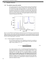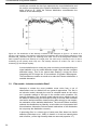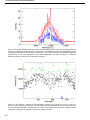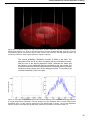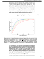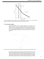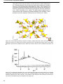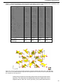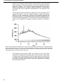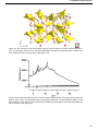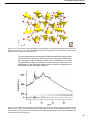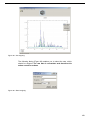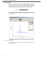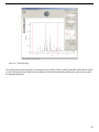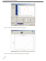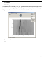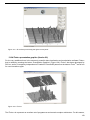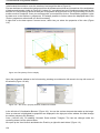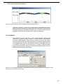
1
Two-dimensional X-ray powder diffraction Der Fakultät für Geo- und Biowissenschaften der Universität Stuttgart zur Erlangung der Würde eines Doktors der Naturwissenschaften (Dr. rer. nat.) genehmigte Abhandlung Vorgelegt von Bernd Hinrichsen aus Tsumeb, Namibia Hauptberichter: Prof. Dr. R. E. Dinnebier Mitberichter: Prof. Dr. P. Keller Tag der mündlichen Prüfung: 7.11.2007 Max-Planck-Institut für Festkörperforschung Stuttgart, 2007 To Christiane, Aurel and Darius Contents Abbreviations 0 Introduction . . . . . . . . . . . . . . . . . 6 . . . . . . . . . . . . . . . . . 7 . . . . . . . . . . . . . . . . . . . . . . . . . . . . . . . . . . . . . . . . . . . . . . . . . 9 . 9 . 12 . 26 1 The experimental setup . 1.1 Two-dimensional detectors 1.2 Diffraction geometry . . 1.3 Corrections . . . . 2 Calibration . . . . . . . . . . . . . . . . . 2.1 The calibration image . . . . . . . . . . . . . . 2.2 Starting parameter estimation . . . . . . . . . . . . 2.3 Parameter refinement . . . . . . . . . . . . . . 2.4 Comparison of methods . . . . . . . . . . . . . . 34 34 34 38 45 3 Intensity distributions and their application to filtering . . . . . . 3.1 Why filter 2D powder diffraction images? . . . . . . . . . 3.2 Detector signal distribution . . . . . . . . . . . . . 3.3 Filter models – inclusive or exclusive filters? . . . . . . . . 3.4 Filter applications . . . . . . . . . . . . . . . 3.5 Conclusion . . . . . . . . . . . . . . . . . 47 47 47 50 51 64 4 Quality assessment . . . . . . . . . . . . . . . 65 4.1 How good are my data? Suggestions for an image reliability value . . 65 4.2 Comparison of reliability values originating from different data . . . . 66 5 Schafarzikite (FeSb2O4) at high pressure . . . . . . . . . 5.1 Abstract . . . . . . . . . . . . . . . . . . 5.2 Introduction . . . . . . . . . . . . . . . . . 5.3 Experimental . . . . . . . . . . . . . . . . 5.4 Conclusion . . . . . . . . . . . . . . . . . 67 67 67 68 75 6 Tin sulphate at high pressures . . . . . . . . . . . . 6.1 Introduction . . . . . . . . . . . . . . . . . 6.2 Experimental . . . . . . . . . . . . . . . . 6.3 Conclusion . . . . . . . . . . . . . . . . . 76 76 76 85 7.1 Précis . . . . . . . . . . . . . . . . . . 87 7.2 Zusammenfassung . . . . . . . . . . . . . . . 89 8 References . . . . . . . . . . . . . . . . . 91 Two-dimensional X-ray powder diffraction Abbreviations If not temporarily defined otherwise within the text the following definitions hold: LP Combined Lorentz and polarization corrections CCD Charge coupled device PSF Point spread function FWHM Full width at half maximum 2q Angle of diffracted beam to primary beam q Half the above angle D Distance of the detector from the sample along the primary beam tilt Maximum angle between the primary beam normal plane and the detector rot Rotation of the tilted plane a Angle of azimuth Y Incidence angle of the diffracted beam on the detector l Semi-latus rectum c Distance between focus and centre of an ellipse a Semi-major axis of an ellipse b Semi-minor axis of an ellipse e Eccentricity of a conic section r Radius L Lorentz correction Introduction 0 Introduction With the general availability of high intensity parallel synchrotron radiation, the use of two-dimensional detectors like CCD-detectors or on-line image plate readers for fast high resolution data acquisition enjoys a growing popularity. As a consequence, the field of X-ray powder diffraction has experienced a renaissance. For the first time it is now possible to record the entire Debye-Scherrer rings up to high angular range with high angular resolution within a few seconds or even less. The field of applications is vast with current experiments including texture analysis (Wenk & Grigull, 2003) and in situ powder diffraction measurements in dependence on pressure (Hanfland et al., 1999), temperature (Norby, 1997), chemical composition (Meneghini et al., 2001), electric and magnetic fields (Knapp et al., 2004) or external strains (Poulsen et al., 2005). The experimenters is faced with two major challenges. Firstly, large area detectors produce large numbers of two-dimensional images which need to be reproducibly reduced to one dimensional powder patterns. Secondly, the sets of hundreds or even thousands of powder patterns need to be evaluated and graphically presented. It is interesting to note that for both tasks only very few generally available programs exist. These are keyed toward single powder patterns involving extensive manual interaction. This approach is unsuitable for mass data analysis: not only is the manual workload exorbitant but the induced subjectivity hinders reproducible results. The key to solve the first problem lies in the reliable extraction of a powder diffraction pattern unaffected by “graininess” effects, detector aberrations, and scattering from other sources like reaction cells, diamond anvils and gaskets. The diffraction pattern from a two-dimensional image can be reduced to a simple geometric figure: the ellipse, calling for the application of modern pattern recognition techniques (Paulus & Hornegger, 1995, Theodoridis & Koutroumbas, 1999) to determine the parameters describing their arcs. As to the representation and evaluation of the integrated powder patterns, a high level graphically powerful programming language offers the basis for an efficient solution. We decided on the Interactive Data Language IDL (ITT-VIS, 2006) to develop a general program for automatic data reduction and the evaluation of two-dimensional powder diffraction data called Powder3D. Various aspects necessary to solve problems encountered during the investigation of crystal structures at high pressure are described here. The geometrical basis of two-dimensional diffraction has been assimilated and transformed to a useful coordinate system. This was most useful as most diffraction corrections functions for two-dimensional data were devised for single crystal diffraction. The effective Lorentz correction for a highly collimated beam was deduced. A calibration method based on pattern recognition was developed to determine the detector position and orientation automatically. These parameters were refined using a new approach termed whole image refinement in which the entire diffraction image is reconstructed, and this used as a basis for the calculation of a least squares residual. This method improves the accuracy of the calibration parameters by more than one order of magnitude. Filtering methods based on fractile filtering have been introduced The intensity distribution of high pressure experiments, which in many aspects deviate from standard powder diffraction experiments, was found to follow a somewhat blurred (due to the detector point spread) Pareto distribution. This distribution Two-dimensional X-ray powder diffraction model was used to develop a method of extracting normally distributed intensities from the image, a fundamental necessity of all minimization routines based on least squares. An image reliability value was devised for quantifying the quality of a powder diffraction image. Two applications of the methodological development are presented. The structural evolution of FeSb2O4 and SnSO4 under extreme pressures. It has been mentioned that high pressure experiments using diamond anvil cell techniques are the most challenging experiments in two-dimensional Xray diffraction, not only in sample preparation, but also in the data analysis. Many results are published without structural Rietveld refinements, as a direct result of the difficulties in extracting reliable intensities from the raw images. That this is routinely and efficiently possible has been shown exemplarily in the presented studies. The tin sulphate experiment shows which precision this method is capable of. Most subtle changes in the symmetry of the crystal structure become apparent after the raw data has been treated accordingly. The experimental setup 1 The experimental setup 1.1 Two-dimensional detectors The first two-dimensional detector in X-ray diffraction was conventional film. It remained for decades the detector of choice for both single crystal as well as powder diffraction experiments. In the field of two-dimensional detection it has been surpassed initially by image plates and later by CCD cameras. Today virtually no film is in use, with perhaps the exception of Polaroid used for single crystal images. To be able to compare various detectors with one another and to select the most appropriate detector for a specific experiment certain key technical qualities are important. These are in general the detective quantum efficiency, the spatial response characteristics, the size, speed and dynamic range (Westbrook, 1999). The detective quantum efficiency (DQE) (Gruner et al., 1978) is a measure of the signal to noise degradation caused by the instrument. It is defined in equation 1.1. 2 I out 2 out 1 DQE 2 2 I in NRout 2 in (1.1) I and σ represent the input (Iin) and output (Iout) intensities and the input (σin) and output (σout) standard deviations of the signal intensities, N is the number of incident X-ray photons and Rout is the relative variance of the output signal. A detector with a DQE of 50% has to count twice the time a detector with a DQE of 100% has to count to record a signal of equal variance. The spatial response characteristics (Ponchut, 2006) are normally characterized by the point spread function (PSF) – the detectors signal to a delta function stimulus. Ideally the point spread is also a delta function. Experimentally this is seldom the case as detector characteristics generally give the signal a Gaussian spread. It is the point spread function which is the main cause of the limited resolution in powder diffraction experiments. The size of the detector is an important factor determining the size of the accessible reciprocal (or q-) space. Larger detectors offer a greater area and thus a greater q-space which can be imaged in one exposure. Greater size also opens the possibility of moving the detector further from the sample to improve resolution. Speed is of ultimate importance when acquiring data at a synchrotron beam line. The readout time should be minimal to ensure a high time resolution for in-situ experiments and a most efficient use of the costly synchrotron rays. The dynamic range of the detector limits the intensity differences that are recordable on one image. The higher the dynamic range the better one is able to characterize signals having a strong contrast. Two-dimensional X-ray powder diffraction Figure 1.1: Detector types. Five different detector designs are shown in their fundamental units. This is an adaptation of an image in Chotas (Chotas et al., 1999). 1.1.1 CCD Detectors Probably the widest spread detector type utilized today in X-ray crystallography is the CCD camera. These detectors are in use in multifarious fields and their general ongoing development has been of benefit to the relatively small X-ray detector segment. The great advantages of these detectors are their high resolution and short readout times. This is of importance especially in single crystal diffraction in which dead times can make up a great part of the measurement time. The drawbacks stem from three basic elements of the detector. The fluorescent screen has to be optimised for the required wavelength. The higher energy radiation requires a thicker layer to fully absorb the incident rays. Thicker layers are disadvantageous as the PSF increases with the strength of the layer. This is due to the spherical dissipation of excited electrons within the fluorescent layer. Fibre optical tapers channel the light from the large fluorescent layer to the smaller CCD chip. The tapering often leads to an imperfect representation of the original image onto the CCD. This has to be corrected as much as possible within the detector electronics (firmware). Some detectors have a CCD area of equal size to the fluorescent layer and can circumvent this source of errors. Finally one major drawback is the substantial dark current from the CCD chip which requires permanent cooling to reduce these effects. 10 The experimental setup 1.1.2 Imaging plate detectors Imaging plates were the first digital technology to replace films in synchrotron and laboratory equipment. The concept is extremely simple. A layer of BaF(Br,l):Eu2+ which contains colour centres, is deposited on a robust film like base ‘plate’. The plate is then exposed to X-rays. The image is later scanned by an online or a more cumbersome offline scanner. Scanning the image comprises exciting the colour centres and then detecting the induced radiation. Stimulating colour centres does not require much energy, generally red lasers suffice. The stimulated green light is detected by a photomultiplier following in the path of the laser. The great advantages of imaging plates are their large size, low cost and their high dynamic range. The latter quality has made it the detector of choice for two-dimensional powder diffraction. Their major drawback is the high dead time associated with the time consuming scanning. This can take the best part of two minutes for large images. Rigaku MSC has developed a practical solution to this problem. The detector system is comprised of two or even three detectors. When one is being scanned the other can be exposed. A precision rotation system transports the imaging plate from one position to the other. The future for this detector type does seem rather bleak especially in view of flat panel detectors and the single photon counting hybrid pixel detectors. 1.1.3 Flat panel detectors Thin film transistor (TFT) arrays are produced inexpensively and in large numbers for use in modern computer monitors and televisions. This readout system can be combined with amorphous hydrated Silicon or amorphous Selenium which is deposited over the large surface of the TFT array and acts as the X-ray conversion layer. Having established themselves firmly as an X-ray detector for medical imaging already, they have until now failed to make an impact on the field of crystallography (Ross et al., 1997), their high noise level being the main drawback. It can be surmised with some confidence that this type of detector will become standard equipment in the near future. A very general categorization into direct and indirect conversion types can be made for these detectors (Chotas et al., 1999). Within direct converters X-rays are transformed to electrons in a single step, for example by a layer of amorphous Selenium. One further step is required for the indirect sensors: here a scintillating layer (photoconductor) converts the X-rays into visible light, which is in turn converted to an electronic charge by a further amorphous Silicon layer. This brings with it the inevitable resolution loss associated with the radial diffusion of photons and again their interaction with the amorphous Silicon. As with all detection layer systems they can be optimized using various layer thicknesses and scintillating substances which can be selected according to the X-ray wavelength and the photon detection properties of the lower layer. Currently vapour grown CsI:Tl as an extremely popular material. It grows in columnar structures and can act as a guide in a similar fashion to fibre optics, thereby reducing lateral scattering. Its high atomic number secures a high X-ray absorption and thus good conversion. Other materials under study as possible photoconductors are HgI2, PbI2 and CdZnTe (CZT). Especially CZT, grown using a high-pressure Bridgeman technique, has been rapidly implemented in a wide variety of medical detectors (Darambara, 2006). 11 Two-dimensional X-ray powder diffraction 1.1.4 Hybrid pixel detectors Silicon pixel array detectors are based, as the name suggests, on Silicon as the primary detecting layer. The photoelectric effect causes one electron/ hole pair to be created for each 3.65eV of incident X-rays. This leads to 3220 electrons from each X-ray photon at 12keV in a one millimetre layer, which absorbs 98% of that radiation. In contrast a CCD would only produce roughly 10 electrons. The readout time of a few nanoseconds also contrasts impressively with all other detector systems. Further no distortions are to be expected as no intermediary tapering or disconnected readout systems are involved. In spite of these overwhelming advantages the price of prototyping and the expense of the readout electronics design has inhibited the speedy development of this detector type. Nevertheless a few groups have been working on realizing a detector specifically for crystallography. Workers around Christian Broennimann (Broennimann et al., 2006, Hulsen et al., 2006) have succeeded in building a one megapixel detector for protein crystallography with a pixel size of 217x217µm². Although this might be larger than the pixels of a CCD the perfect point spread function of a single pixel still represents a marked resolution improvement over the CCD detector types. The detector was built up of an array of 18 modules covering a total area of 210 x 240 mm². A full frame readout time of this detector takes 6.7 ms allowing a continual rotation single crystal data collection without the shutter closing between frames. Detectors of this type are already in operation (Fauth et al., 2000) in the field of powder diffraction. Large manufacturers of diffraction equipment have these detectors among their products, disappointingly reduced to point detectors and not implemented as area detectors. An installation at the material science beam line at the Swiss Light Source (SLS) of the Paul Scherrer Institute (PSI) in Switzerland is an equatorial type detector, covering a fixed angle of 60° in 2θ. This is again no real two-dimensional detector. It has a faster readout time than the two-dimensional detector mentioned earlier and can acquire entire diffractograms in a fraction of a second. Most probably this type of detector will establish itself in the field of two-dimensional diffraction. 1.2 Diffraction geometry Early powder diffraction experiments relied mostly on the Debye-Scherrer experiment to record a diffractogram. A broad film strip set into a cylindrical chamber produced the first known two-dimensional powder diffraction data. In contrast to modern methods the thin equatorial strip was the only part of interest and intensities merely optically and qualitatively analysed. This changed drastically with the use of electronic scintillation counters. Intensities were no longer a matter of quality but quantity. Inevitably the introduction of intensity correction functions long known to the single crystal metier i.e. Lorentz and polarization corrections (see page 22), made their way into the field of powder diffraction. Continuous detector development brought about the next revolution in the field of powder diffraction. Large area detectors made their debut in powder diffraction at synchrotron beam-lines in the beginning of the nineties, having first been used in the field of single crystal diffraction. First experiments only utilized thin equatorial strips (Norby, 1997) of the image but with the introduction of freely available software (Hammersley et al., 1996), the integration of the entire image to a standard one-dimensional powder diffraction pattern became commonplace. 12 The experimental setup The term two-dimensional powder diffraction does not imply any specific geometry; it merely states the two-dimensionality of the detected signal. It could be conceived that this detector be cylindrical as in a Weissenberg camera. Such detectors are still common in modern single crystal diffractometers in both standard laboratories (Rigaku, 2004) as well as at neutron beam-lines (Cole et al., 2001); however the concept has never gained great popularity in the modern powder diffraction field. The ubiquity of large flat image plate detectors, their unparalleled dynamic range as well as a speedy read-out time are the reasons for their current prominence in the field. A precise determination of the experimental geometry is a prerequisite for highly accurate and well resolved diffraction angles, peak profiles, absorption effects or even good filtering. Especially the separation of microstructural effects from the instrumental contribution to the peak profile needs exact 2θ values. An accurate calibration remains the single most significant factor in the extraction of high quality powder diffractograms from two-dimensional images. Generally the detectors are set up perpendicularly to the primary beam, with the intersection of the primary beam at the detector centre. This setting has some advantages: the entire Bragg cones are detected and the deviation of the cone projection from an ideal circle is usually small. Sometimes a detector can be placed off-centre and non-orthogonally to the primary beam. This can enlarge the detectable q-space in a very cost effective manner. The down-sides are the strongly elliptical conical projections and the loss of the entire azimuthal information of a diffraction cone. Extraction of standard powder diffractograms from two-dimensional images requires knowledge of the diffraction angle at each pixel. These angles have to be known to a precision equal to or less than the detector resolution. The detector resolution is mainly governed by the point spread function (PSF). In addition the calculation of air absorption would require the sample to pixel distance in each case. The azimuthal angle is vital for the application of the Lorentz and polarization corrections as is the incident angle for a detector dependent correction. The following chapter will deal with the derivation of all possible geometrical values which could be of importance during data reduction. 1.2.1 Resolution and FWHM in two-dimensional diffraction The resolution of a two-dimensional detector is governed to a dominant extant by the PSF. This can be very well observed by the behaviour of the FWHM distribution of reflections over an image plate. The PSF of a standard image plate is roughly 300µm. The projection ∆l of the diffracted beam width d on the image plate in the case of a fully parallel beam is given by: d l cos( ) This would result in the projection of the diffracted beam leaving a larger footprint on the image plate at higher incident angles (Ψ); we should therefore expect higher FWHM of the diffracted beams at higher incident angles. Experimentally we find an inverted relation. How can this seemingly aberrant behaviour be explained? The answer lies in the PSF 13 Two-dimensional X-ray powder diffraction of the detector. Detectors do not resolve differences in the half-width of the incident beam if they lie well below the point spread of the detector. The increasing footprint of the incident beam is overshadowed by the detectors point spread, thus leading to no discernable effect. So it is no surprise that with changing incident angle and sample distance the ‘number of points (pixels) across the peak … is not changed’ (Norby, 1997). The reduction in the FWHM of the diffracted X-rays at higher incident angles is more intrinsically connected to the angular resolution per pixel (figure 1.2). Figure 1.2: The effect of the incident angle on the sharpness of the final angular projection. The point spread of the detector does not change. The difference in the angular resolution between the perpendicular and the tilted detector is the cause of the sharper peak. Taking into account both the effect of the incident angle and the distance of the detector from the sample the resolution of an experimental setup can be calculated as the half-width (FWHM) of the diffracted beam by its diffraction angle (2θ), the PSF of the detector and the sample to detector distance (D). For simplicity we assume that the detector tilt is negligible. The radius is then related to the sample detector distance and the diffraction angle by the following equation (see figure 1.8): D tan 2q r (1.3) Adding the FWHM and the point spread contribution would lead to: D tan(2q FWHM ) r PSF (1.4) As equation 1.3 still holds 1.4 would become: D tan(2q FWHM ) D tan 2q PSF Solving for FWHM in terms of 2θ and the PSF then leads to: 14 (1.5) The experimental setup D tan 2q PSF FWHM arctan 2q D (1.6) To show the effect of the PSF on the FWHM of a diffracted beam a surface spanning a 2θ range from 0° to 70° and a detector distance range from 100mm to 1000mm has been calculated, estimating the point spread to be 300µm (figure 1.3). Figure 1.3: The effect of the point spread of a two-dimensional detector upon the FWHM of a diffracted beam is represented. The detector is assumed to be ideally aligned normal to the primary beam. The point spread is taken to be 300µm. Sample contributions to the peak width have not been considered. The effect of the diffracted beam projection onto the image plate 1.2 has not yet been included into the FWHM calculation. Adding this factor to the broadening leads to the following estimation 1.7, again for an idealized non-tilted detector. To verify the applicability of this estimation the theoretical values have been plotted against experimental data from a calibration image(see Figure 1.4). The image had a minimal tilt of 0.2°, the sample to detector distance was 141 mm, the diffracted beam was 0.2 mm and the point spread was estimated to be 0.32 mm. D tan 2q PSF d *sec 2q FWHM arctan 2q D (1.7) 15 Two-dimensional X-ray powder diffraction Figure 1.4: Calculated full width at half maximum (FWHM) and observed FWHM for a calibration image of LaB6 are plotted against one another. The solid line represents the calculated values, whereas the crosses represent the measured values. To calculate the theoretical values the diffracted beam width was taken to be 0.2 mm the point spread of the detector was set to 0.32 mm and the sample to detector distance was taken as refined by the calibration at 141 mm. It is possible to estimate the line width of an orthogonally aligned diffraction experiment by knowing the width of the diffracted beam, the PSF of the detector and the distance to the detector. Adding tilt to the two-dimensional detector makes the situation a lot more complicated. Essentially an azimuthal factor is added to the incident angle as well as to the angular resolution. This results in an azimuth dependent FWHM of the diffraction image. The dependence of the line width on the detector orientation is given in its complete form by equation 1.8. This equation is deduced in the same manner as equation 1.6, however starting from the more complex formulation of a tilted detector given by equation 1.12. FWHM arctan xPSF cos(rot ) yPSF sin(rot )2 cos 2 (tilt ) yPSF cos(rot ) xPSF sin(rot )2 2 D xPSF cos(rot ) yPSF sin(rot ) sin(tilt ) x cos(rot ) y sin(rot )2 cos 2 (tilt ) y cos(rot ) x sin(rot )2 arctan , 2 D x cos(rot ) y sin(rot ) sin(tilt ) xPSF x PSF , yPSF y PSF For a precise explanation of the terms rot and tilt please refer to figure 1.9 and figure 1.11. The line width can also be expressed in the more general terms of diffraction angle (2q), azimuthal angle (a), detector orientation (D, rot, tilt) and the detector point spread (PSF). To deduce the formula we start with equation 1.3 but alter it to fit a tilted detector. This implies adding a distance z to the sample to detector distance. It represents the change of the distance to the reflection point on the detector projected onto the primary beam vector. This change is brought about by the tilt and can easily be derived as is shown in Figure 1.10a. The factor narrowing the effective width of the tilted beam (figure 1.2) has to be added, leading to modified form of equation 1.5. 16 (1.8) The experimental setup Figure 1.5. A theoretical two-dimensional diffraction pattern. Notice the effect of the broadening by the incident angle and the point spread function on the pattern. The high density of diffraction lines in the bottom left is caused by the extreme tilt (45°) of the detector. D z tan 2q FWHM cos tilt cos a D z tan 2q PSF (1.9) The change in distance is given by the following equation: z r sin(tilt ) (1.10) The radius has been derived and is given by equation 1.37. Substituting all values of z and r in equation 1.10 and equation 1.9, solving for the FWHM and simplifying leads to the fundamental formulation of equation 1.9. num FWHM arccot sec tilt cos a 2q , den num D D cos a cos tilt tan tilt tan 2q , (1.11) D D sin tilt tan 2q den PSF tan 2q cos a tan tilt PSF D tan 2q Such a situation can be simplified if only a thin Debye-Scherrer type strip along an azimuthal angle is considered (Norby, 1997). The effects of diffracted beam projection and the point spread function on the image can be seen in figure 1.5. This figure displays a theoretical image of LaB6, setting the detector at a tilt as well as a rotation angle of 45°. At large incident angles the beam projection contributes most to the line broadening, while at low incident angles both contribute to the line broadening. The projection of this image into reciprocal space Figure 1.6 is enlightening. When compared to the initial pattern used to generate the image it can be clearly seen how the line width alters for different peaks. Instead of the typical orthogonal setup behaviour in which the line width diminishes with higher diffraction angle because of its equivalence to the incident angle, a non-orthogonal detector can give peak widths that broaden at higher diffraction angles. 17 Two-dimensional X-ray powder diffraction Figure 1.6. A comparison of the initial pattern (black line) used to generate a two-dimensional image and the integrated pattern from the image (in red).The detector was highly tilted leading to a large difference in the incident angle between the low angle peaks, which had large parts of their arc at high incident angles, and the high angle peaks had low incident angles, leading to greater peak widths. The reason why the peaks at low diffraction angles are still so much narrower than those at high angles although parts of their ellipses are in a region of low incidence is simple. The fraction of their ellipse arc at low incidence angles is relatively small, the majority of the arc lies in a region of high incidence and therefore this dominates the signal. The difference in peak width becomes quite clear when the peak width at different azimuthal angles is viewed figure 1.7. The high incident angle region in this case lies at an azimuth of 45°. The low incidence angles lie diametrically opposite. When using focusing optics (von Dreele et al., 2006) the detector distance to the optics is fixed and the focal spot of the beam well below the PSF of the detector. The resolution is governed solely by the PSF of the detector. To decrease the resulting line width the only solution is to increase the distance between the sample and the detector, as tilting the detector would move it out of the focal point. Figure 1.7. The effect of extreme detector tilt on the line width at different azimuthal angles. A point spread of 300µm and a detector tilt of 45° has been the basis of this computation. 18 The experimental setup 1.2.2 Diffraction angle transformation The fundamental function relating the non-orthogonality of the detector to the primary beam and the sample to detector distance into diffraction angles is given by 1.12. This equation can easily be deduced from two rotations of the plane out of its position orthogonal to the cones axis. The first rotation is performed around the x-axis. As can be seen in figure 1.8 it causes the conic section to become elliptical. The axis of the cone now intersects the plane at a focal point of the ellipse. What was the radius in the circular conic section now has become the semi-latus rectum figure 1.13. A second rotation is performed around the plane normal centred on the focal point which is the intersection of the cones axis. The effect of this rotation is shown in figure 3. This transformation provides a general formulation of a conic section using experimentally accessible parameters. 2q arctan 2 2 cos 2 (tilt ) x cos(rot ) y sin(rot ) x sin(rot ) y cos( rot ) 2 D sin(tilt ) x cos(rot ) y sin(rot ) (1.12) The parameters x, y, tilt, rotation and D are depicted in figure 1.8 to figure 1.11. A deduction of this equation has been given by (Hammersley et al., 1996) and is described with the aid of figure 1.8 to figure 1.11. (Kumar, 2006) gave a good overview of the transformations involved in calculating the conic section. He however chose to use three angles to describe the detector orientation relative to the scattering cone. As any detector orientation can be described by two angles alone, this is the transformation we chose to use. Figure 1.8: A circular conic section resulting from an orthogonal detector to primary X-ray beam setting. On the left is a view perpendicular to the detector, on the right is a side view, showing the primary beam entering from the right. The primary and diffracted beams from the sample S intersect the detector on the detector plane. The primary beam intersects the detector at the centre of the circle. For clarity only one diffraction cone has been drawn. The distance from the sample to the detector along the primary beam is given by D. The detector coordinate system is denoted in x and y relative to the beam centre. 19 Two-dimensional X-ray powder diffraction In figure 1.8 a conic section normal to the cones axis is displayed. The diffraction angle, which is half the cones opening angle, is given by equation 1.13. All the coordinates are given in the cone coordinate system wherein z is the cones axis, and x and y describe the plane perpendicular to it. The position of the plane is at a distance D from the cones apex along the cones axis. x 2 y 2 D 2 tan 2 2q (1.13) In our case the cones axis is synonymous with the primary beam. For the conic section to change from a circle to an ellipse the angle between the plane normal and the cones axis has to be greater nought. Dx cos(tilt ) 2 2 Dy 2 2 D tan 2q D x sin(tilt ) D x sin(tilt ) (1.14) This is realized in figure 1.9 and figure 1.10 by rotating the cones axis around the horizontal plane axis, this is equal to the x-axis. For sake of compatibility with the established formulation (Hammersley et al., 1996) the detector is tilted around the y-axis. The coordinate system changes to that of the tilted detector and is denoted by x’ and y’ (figure 1.10). Figure 1.9: The elliptical conic section resulting from a tilting of the detector around a horizontal axis. This results in an ellipse which is mirror symmetrical along the central vertical axis. The equation 1.14 then simplifies to 1.15. 2 x2 cos 2 (tilt ) y2 D x sin(tilt ) tan 2 2q 20 (1.15) The experimental setup Figure 1.10: Constructions after Kumar (Kumar, 2006) to deduce the tilted x’ and y’ values in terms of the orthonormal x and y values. Image a) shows the construction used to calculate the relation between x and x’. The similarity of the triangle spanned by D and x (small triangle), and the triangle spanned by D+x’sin(tilt) and x’cos(tilt) is used to set up the relation. Image b) shows the construction used to elucidate the relation between y and y’. Here again the similarity of the smaller and larger triangles are used to set up the relation. Adding a rotation angle around the normal to the focus of the ellipse leads us to the general ellipse represented in figure 1.11. Figure 1.11: The general description of an arbitrary tilt. The added rotation angle suffices to describe any possible detector tilt. This adds a cosine and a sine term of the rotation to the x and y values in the following form. Again a separate notation is used to denote the rotated values x’’ and y’’. 21 Two-dimensional X-ray powder diffraction x x cos( rot ) y sin(rot ) y y cos( rot ) x sin(rot ) (1.16) On inserting these rotational equations into equation 1.15 one obtains the equation 1.17. x cos(rot ) y sin(rot )2 cos 2 (tilt ) y cos(rot ) x sin(rot )2 2 D x cos( rot ) y sin(rot ) sin(tilt ) tan 2 2q (1.17) Equation 1.6 can be rearranged to the initial form equalling equation 1.12. x cos(rot ) y sin(rot )2 cos 2 (tilt ) y cos(rot ) x sin(rot )2 2q arctan (1.18) 2 D x cos(rot ) y sin(rot ) sin(tilt ) 1.2.3 Incident angle and ray distance calculations The incident angle of the reflected beam onto the detector is utilized in a factor often described as correcting for the flatness of a detector. The diffracted beam penetrates into the image plate or fluorescent layer of the detector. The penetration length is dependent on the angle of incidence and the linear attenuation factor for the utilised wavelength and fluorescent material. Figure 1.12: Incident angle calculation. The small triangle containing the complementary angle to the incident angle Ψ and tilt is used to deduce the formula for the calculation of the incident angle. As can be seen from figure 1.12 the minimum and the maximum incident angle are given by the following equation 1.19. 22 The experimental setup min 2q tilt max 2q tilt (1.19) The tilt can be replaced with the effective tilt, tilt eff according to: tilteff tilt sin(a rot ) (1.20) Resulting in an effective incident angle of: eff 2q tilt sin(a rot ) (1.21) To determine the distance of the diffracted ray from the sample to the each point on the detector we use the construction presented in figure 1.12. The application of the sine rule results in the following equation: sin(90 ) sin 180 2q (90 ) D ray distance (1.22) ray distance D cos 2q sin 2q tan (1.23) This simplifies to: 1.2.4 General transformations As most pattern recognition algorithms use conventional geometric parameters of ellipses, namely semi-major and semi-minor axes and eccentricity, the following chapter will deduce all the necessary transformations between the crystallographic and standard system. Further transformations are needed to calculate the exact Cartesian coordinates of a reflection on the detector. This corresponds to the determination of x,y=f(2θ,α, D,tilt,rot,X0,Y0). This information is important for calculating and plotting theoretical ellipse positions. The semi-latus rectum l is independent of the tilt and can be given in terms of the scattering angle and the sample to detector distance as in equation 1.24. D tan 2q l (1.24) From figure 1.12 and the sine rule we can deduce the following relation sin(2q ) sin(90 2q tilt ) a c D (1.25) c a D sec(tilt 2q ) sin 2q (1.26) This can be reformed to 23 Two-dimensional X-ray powder diffraction Figure 1.13: Common ellipse parameters. The centre is denoted by C, one focal point by F, the semimajor axis by a, the semi-minor axis by b and the semi-latus rectum by l. However we also know from figure 1.12 and the sine rule that the following relation holds. sin(2q ) sin(90 2q tilt ) a c D (1.27) c a D sec(tilt 2q ) sin 2q (1.28) This can be reformed to Setting equations 1.26 and 1.28 equal and solving for a leads to the following formulation: D cos(tilt ) sin 4q a cos( 2tilt ) cos 4q (1.29) The same method can be used to find an expression of c in alignment variables. This leads to the very similar formulation 2 D sin(tilt ) sin 2 2q c cos( 2tilt ) cos 4q (1.30) al b 2 (1.31) Because of the well known identity 1.31 the semi-minor axis can be described using the scattering angle, the tilt and the detector to sample distance, as given in equation 1.32. 24 The experimental setup D cos(tilt ) sin 2q tan 2q cos( 2tilt ) cos 4q b (1.32) Now a and c can be inserted into the well known identity e=c/a to denote the eccentricity in calibration parameters. tan(tilt ) tan 2q e (1.33) 1.2.4.0.1 Detector coordinate transformations We will now attempt to deduce the detector coordinates from the calibration values and the reflection parameters. Some well known elliptical identities 1.34 and 1.35 shall be used in these calculations. b2 e 1 2 a (1.34) c a 2 b2 (1.35) The ellipse radius as measured from the focus can be described in terms of eccentricity, semi-major axis and the angle of the azimuth 1.36. rfocusellipse a (1 e²) 1 e cos(a ) (1.36) Inserting equations 1.34 and 1.35 into the equation 1.36 leads to: rfocusellipse D tan 2q 1 cos a tan(tilt ) tan 2q (1.37) The Cartesian coordinates take the following values: yd rfocusellipse sin(a rot ) (1.38) xd rfocusellipse cos(a rot ) (1.39) Here xd and yd are the x and y positions relative to the focus. The ellipse has been made non-parallel to the axes by subtracting the rotation from the azimuth angle. 25 Two-dimensional X-ray powder diffraction 1.3 Corrections 1.3.1 Intensity corrections As important as the diffraction angles are to the exact lattice parameters, the intensities are for the precise determination of atomic position, elemental species, and their occupation and displacement parameters. The great popularity of equatorial point detectors and later one dimensional position sensitive detectors in laboratory diffractometers has hindered the spread of generally applicable correction formula and canonized equatorial specific corrections. These are often incorrectly applied to data collected from two-dimensional detectors. Important experimental factors influencing the intensity of a diffracted beam are discussed and the corresponding twodimensional correction functions are given. 1.3.1.1 Lorentz corrections Lorentz correction applied to powder diffraction data are slightly different to those applied to single crystal data. Whereas the single crystal correction only comprises a rotational factor, the powder correction contains an additional statistical factor (Zevin, 1990). This corrects for the likelihood of a crystallite being in diffraction position. This factor has a simple (sinθ)-1 dependence, and is found in the common Lorentz correction 1.40. L1 sin 2q sin q (1.40) The well known correction for the speed of the transition of a reflection through the Ewald membrane is attributed to a lecture given by Lorentz (Azaroff, 1968). In its form applicable to a perfect single crystal it normalizes the intensity of a single reflection to the shortest traversal of the Ewald sphere. This motion is brought about by the rotation of the crystal in direct space. A consequence is that the correction is not only dependent upon the rotation vector of the crystal but also on the detection method. The general formulation (McIntyre & Stansfield, 1988) takes the form: 2 Fhkl µ (dz / ds ) I xy ( s )ds (1.41) Here Ixy is the reflection intensity measured as a function of a scan variable s. z is the direction normal to the Ewald sphere at the reflection position. Integrating over s for a typical four-circle diffractometer (Busing & Levy, 1967) and approximating sine and cosine values for the small angular range of a reflection leads to the following formalism: i sin cos i sin sin L1 cos sin cos cos sin sin i (1.42) When regarding rotation around a single axis, an experimental set-up most commonly used in two-dimensional powder diffraction the function reduces to (Buerger, 1970): L1 cos sin cos 26 (1.43) The experimental setup Where µ = angle between axis of sample rotation and the primary beam normal plane, γ = angle of horizontal reflection displacement and ν = angle of vertical reflection displacement. The well known equatorial form of equation 1.43 is obtained when setting the axis of rotation perpendicular to the primary beam and reducing the vertical displacement to nought, γ is then the diffraction angle. L1 sin 2q (1.44) The reduction from the two-dimensional form to the one-dimensional equatorial form was a requirement of the equatorial diffractometer geometries utilizing point detectors or at most linear position sensitive detectors. It is important to note that this correction is neither applicable to the Bragg-Brentano nor to the flat transmission geometry, but is only valid for the Debye-Scherrer geometry. With the onset of area detection in powder diffraction a two-dimensional correction has to be applied. A formulation of 1.43 in dependence on the more accessible scattering angle 2θ and the azimuthal angle α has been derived: L1 cos cos a tan 2q 1 cos 2 a tan 2 2q 1 sin 2 a tan 2 2q (1.45) Combining this with the statistical factor leads to the general formulation of the Lorentz correction for powder samples rotated within the beam. L1 sin q cos cos a tan 2q 1 cos 2 a tan 2 2q 1 sin 2 a tan 2 2q (1.46) Figure 1.14: The two-dimensional single crystal Lorentz correction for an ideally aligned detector. Note the zero values in the central valley. These cause divergent intensities as they are multiplied with the inverse of the Lorentz correction. Therefore the intensities in that region have no meaning. The central valley is parallel to the sample rotation axis. 27 Two-dimensional X-ray powder diffraction 1.3.1.1.1 Lorentz correction for highly collimated beams The rotational correction should be used if the powder sample is rotated within the beam in the single crystal sense i.e. all crystallites should complete their rotation within the beam. Should the beam be collimated to dimensions below those of the sample containment then this further reduces the rotational impact on the cumulative Lorentz factor. A term RL can be introduced to quantify the rotational Lorentz factor from 0 for no rotational element to 1 for full rotation of all crystallites within the beam. The introduction of this factor leads to equation 1.47. L1 sin q RL cos cos a tan 2q 2 1 cos a tan 2 2q 1 sin 2 a tan 2 2q (1.47) RL has been deduced for the case of the rotational axis being normal to the primary beam. The common Lorentz formulation is valid if a crystallite is rotated within the beam by ω =2π. For a certain number of crystallites with a rotational radius less than the beam radius this is true. Crystallites outside this radius experience a rotation ωeff which is dependent upon their rotational radius and the width of the primary beam. It can be given as eff 4 arcsin W R (1.48) where W is the beam width and R is the rotational radius. As all crystallites between R=W and R=L (where L is capillary diameter) are affected differently by rotational radius an integration over that range has to be made. 1 eff eff y dy 2 2 1 y 2 2 y arcsin y , y W L y (1.49) Interestingly the integration tends to a value of roughly 33° as the beam width to sample radius ratio tends to nought. 1 lim eff y dy 2 1 y 0 y (1.50) Now this rotation needs to be put into relation to the entire illuminated area. The normalization takes the form of the average rotational angle of the entire illuminated area relative to the full 2π rotation of standard Lorentz correction. RL 2 f eff f 2 f f Where f is the area in which the crystallites experience a complete rotation in the collimated primary beam and fω is the area in which the crystallites only experience a partial rotation within the beam figure 1.16. These are computed in the following manner: 28 (1.51) The experimental setup Figure 1.15: Relative Lorentz factor. The image depicts a perpendicular section of a capillary of diameter L being illuminated by a beam of width W. Only crystallites falling in the light grey inner circle are rotated completely (2π) within the beam. Crystallites outside this region but still within the beam path only experience a limited rotation ω thus reducing the effective single crystal Lorentz factor to be applied to them. W A 1 4 L2 cos1 W L2 W 2 L f 2 W 2 2 (1.52) (1.53) 2 f 2 L 2 f 2 A (1.54) Reforming equation 1.54 and simplifying leads to 1.55. W f 1 2 L2 W W L2 W 2 L2 cos1 L (1.55) Equation 1.51 then becomes RL 2 f eff f 2 2 2 L 2 2 A (1.56) When reduced to the fundamental parameters the function takes the final form of 1.57: W 2 W arcsin 2 W 1 2 W L 2 2 2 2 2 W L W W L W L arccos 2 1 2 L 4 L L RL W L2 W L2 W 2 2 L2 arccos L 29 Two-dimensional X-ray powder diffraction Figure 1.16: Relative Lorentz factor. The image depicts the trend of the correction factor for a primary beam that is collimated to below the sample size, which is given by S. Should the primary beam be larger than the sample, the factor is unity. In order to see the effect this correction factor has for differing beam sizes and capillaries a simple two-dimensional plot has been made. In figure 1.16 you see that as the beam size approaches zero so does RL approach zero, whereas when the beam size equals or is larger than the sample diameter the standard correction factor of unity is applied. 1.3.1.2 Polarization correction When X-rays are diffracted by a lattice plane they are partially polarized. This leads to an intensity reduction that can be expressed as a function of the diffraction angle. For a completely unpolarized primary beam this leads to the following correction (Lipson & Langford, 1999): 1 1 cos 2 2q 2 P (1.58) Should the primary beam be polarized this changes the correction to (Azaroff, 1955, 1956, Kahn et al., 1982, Whittaker, 1953): P P0 P 1 1 cos 2 2q 2 (1.60) 1 cos 2a sin 2 2q 2 (1.61) P0 P where 30 (1.59) The experimental setup Figure 1.17: The two-dimensional polarization correction for an ideally aligned detector. The polarization factor has been set to 0.1 resulting in the black dome shaped surface and to 0.99 which results blue saddle shaped surface. The correction is applied by dividing the intensities by the displayed correction values. I I I I (1.62) Here Iπ and Iσ are the vertical and horizontal intensities respectively. The monochromator angle is related to µ by the following equation. cos 2 2q m (1.63) With knowledge of the monochromator angle (2θm) and that of the initial polarization of the X-ray beam one can calculate the effective polarization factor. However it is possible to refine this parameter against twodimensional reflection intensities, and thereby retrieve a reliable value. In figure 1.17 one can see the effect of the polarization correction for two different polarization factors. 1.3.1.3 Incident angle correction An intensity correction based on the angle at which the reflected beam strikes the detector plane was initially proposed by Gruner (Gruner et al., 1978) in his work on CCD detectors. Since then the development of this correction has been mainly driven by electron density researchers striving to attain high quality intensity data from area detectors. From figure 1.18 it becomes clear how the incident angle affects the path of the beam through the detecting layer. The distance traversed by the beam in the detecting layer is d/cosΨ, where Ψ is the incident angle and d is the thickness of the detecting layer. 31 Two-dimensional X-ray powder diffraction Figure 1.18: Incident angle correction. The path of the incident ray through the detecting layer of thickness d depends upon the incident angle Ψ. The length traveled within the layer is then d/cosΨ. This correction is necessary should the beam not be completely absorbed by the layer. Reflections at high incident angles would have a falsified higher intensity because of the greater detection length. This correction attempts to normalize the intensity to an incident reflection normal to the plain. If the absorption of the visible light generated within the layer is disregarded then the correction (Zaleski et al., 1998) is independent of the detector type (CCD or IP). K d cos 1 e 1 e d ln T cos (1.64) 1 e 1T with I corr I obs K (1.65) and T↓ being the transmission of the detector layer at normal incidence. This leads to the complete correction function of: I I obs 1T ln T cos 1 e (1.66) An empirical correction that is used by some single crystal diffractometers equipped with CCD cameras takes the following form: K 1 m(1 cos ) 32 (1.67) Calibration Figure 1.19: Incident angle correction factor. The correction factor of (Zaleski et al., 1998) has been calculated for an incident angle range from 0° to 90° and for a vertical transmission ratio from T=0 to T=1. The correction is applied by dividing the observed intensities by correction factor K. The correction factor remains unity for complete X-ray absorption (T=1) as well as for incident angles of 0°. Here m is a coefficient that parameterizes a detector-wavelength combination. For example a CCD detector optimized for copper radiation used m = 0.1763. One optimized for Molybdenum radiation had m = 0.3274. No deduction of this formulation has to date been published. The correction implemented in the Fit2D package (Hammersley et al., 1996) is given by 1.7. Again no formal deduction of this correction has been published. K cos3 (1.68) A more complex function for imaging plates taking into consideration of the additional absorption of the excitation and emitted light has been proposed (Tanaka et al., 2005). I Ff ( x, y, z , , , ) kI zx I y µ µ µ kI ( x, y ) exp g cos p cos y cos z p (1.69) This was reported to provide a better normalization when applied to single crystal data collected for electron density studies of CeB6. In this equation µg, µp and µy represent the linear absorption coefficients of the excitation, X-ray and emitted light within the image plate layer. The corresponding incident angles are ν, κ and Ψ. The vector of the incident X-ray is given by z. 33 Two-dimensional X-ray powder diffraction 2 Calibration The calibration of a two-dimensional diffraction image is the most fundamental step in the process of the reduction of two-dimensional powder diffraction data. The distance of the sample to the detector, the position of the primary beam on the detector, the parameters of the detector tilt and the X-ray wavelength have to be known to the highest possible precision. Only if these values have been determined well can the single pixels of the image be tagged with reliable diffraction angle values. If the calibration has been done optimally the resulting integrated diffraction pattern will not suffer from unnecessary reflection broadening. Especially those reflections contributing large arcs to the images are sensitive to precise calibration values. In addition filtering routines pose high demands on the calibration quality. 2.1 The calibration image All calibrations of powder diffraction images begin with the exposure of a calibration image. This image should be of the highest attainable quality as it is the foundation for the data quality of the final diffractogram. It is advisable to utilize as much of the dynamic range provided by the detector as possible, and to achieve high contrast between the diffraction ellipses and the background intensity. The second step is the manual selection of the inner ellipse; at least five points are required to determine the ellipse parameters (Hammersley et al., 1996). The diffraction image should show well defined solid uninterrupted ellipses, with, if possible, no aberrant intensities. Images from standard samples as those distributed by the NIST (NIST, 2006) produce satisfactory results. However the preparation of an own standard sample is relatively simple. There are a few properties that determine the applicability of a crystalline powder as a calibration standard. The compound should possess a high symmetry, leading to highly intense and well distributed peaks. The composition should comprise strongly scattering, high atomic number elements so that even a sample of small volume can produce a strong signal. A small monodisperse grain size as well as only small contributions from micro-structural (crystallite size and micro-strain) effects guarantee well defined peak profiles. Substances that fulfil these requirements and that are often used for calibration images are LaB6, CeO2 and Si (figure 2.1). 2.2 Starting parameter estimation The calibration refinement is a local minimization. For the refinement to produce a reliable calibration the starting parameters need to be close to the final true values. The most widely used method is the manual selection of at least five points on the inner ellipse of the calibration image. An ellipse is fitted to the points (Fitzgibbon et al., 1999) and the extracted calibration parameters are used to provide the initial estimation (Hammersley et al., 1996). An automatic method has been proposed by Cervellino (Cervellino et al., 2006). They have presented a method to reduce 2D diffraction data, providing both a mechanism to calibrate as well as to integrate such data sets. Another approach is to use traditional pattern recognition methods to estimate the initial parameters. 34 Calibration Figure 2.1 Three calibration images of varying quality are shown. The left image is a good example of a perfect calibration image, utilizing a fine-grained rotating sample of LaB6. The central image is one of a stationary sample of CeO2. Here shadowing causes a slight deviation in the background intensity and the lack of rotation leads to a non-normal intensity distribution within the rings. However the rings are continuous and intense and the detector can still be well calibrated using this image. The right image is again one of a stationary sample, this time of Si. The coarseness of the sample results in an extremely discontinuous intensity distribution along the rings. In addition there is a strong signal at low angles from the capton foil holding the primary beam stop. These factors results in a less stable and less reliable calibration. 2.2.1 The Cervellino method The calibration routine presented requires the sample to detector distance and wavelength to be well defined using alternative methods. A simulated annealing algorithm is used to determine the beam centre. The cost function utilized is the inverse normalized variance of the radial distribution function. In effect this value gives the ‘sharpness’ of the integrated peaks for a trial beam centre, ignoring the effects of detector tilt. The temperature parameter for the simulated annealing is the domain size of the trial beam centre. In the second step the tilt and rotation of the detector are approximated. Certain high intensity ellipses are selected and their inverse squared radii as a function of the azimuth are fitted to a summation of three exponentially damped complex sinusoids. The fitting routine is a modification of the robust singular value decomposition (SVD) method called Hankel Lanczos SVD (Press et al., 1992). A Hankel matrix is filled with parameters from the summation and solved by SVD using the fast Lanczos bidiagonalization algorithm. The refined parameters from the summation can be directly used for calibration. The advantage of this method is that it returns reliable calibration values for a detector that has a near orthogonal setting to the primary beam. It could become a standard method especially for laboratory experiments using radiation of a well defined wavelength, in which the diffracted beam has a substantial half-width. It is however questionable whether the centre estimation suffices to locate the detector/beam intersection with enough precision to calibrate synchrotron data sets. The doubts stem from the difference between the ellipse centre and the confocus of the ellipses, which is the true intersection of the primary beam with the detector (Norby, 1997). 35 Two-dimensional X-ray powder diffraction 2.2.2 Pattern recognition To overcome the first hurdle of finding precise starting parameters, we have developed a robust method for the automatic detection and characterization of ellipses. The method involves no mathematical complexity and exhibits excellent overall efficiency. 2.2.2.1 Ellipse detection An ellipse can be described by five parameters, the major axis a, minoraxis b, centre co-ordinates x0 and y0 and angle of rotation. A widely used pattern recognition technique used in image analysis is the Hough transformation. This has been applied lately (Bennett et al., 1999, Dammer et al., 1997, Fitzgibbon et al., 1999, Lei & Wong, 1999) to ellipse detection in an attempt to facilitate computer vision and biometrics. The first step in a Hough transformation is setting up a parameter space. The dimensionality of the space corresponds to the number of parameters that are to be determined. The size of a dimension depends on the resolution and range required by the corresponding parameter. Parametrical requirements dictate the volume of the parameter space. The next step is to transform the image into the parameter space. This is done by tracing the pattern described by a single pixel in parameter space over the real image. The value of all image pixels touched by the traced pattern are summed and then written to the pixel in parameter space. It is immediately obvious that this process scales with the volume of the parameter space. Reducing the number of dimensions, the required resolution and the range can greatly improve the processing time. Computing all five parameters simultaneously using a Hough transformation is to computationally expensive (Bennett et al., 1999). In order to diminish the size of the required parameter space, the complete process of ellipse detection is decomposed into different steps. The Hough transformation is used for the calculation of the parameter b alone. Hence we require only a one-dimensional parameter space. Figure 2.2. The intensity along a grid line of a powder diffraction image made for calibration purposes. The original image and the overlaid grid are shown in the top right corner. 36 Calibration 2.2.2.1.1 Approximate centre determination Many methods have been used for the determination of the centre of an ellipse (Dammer et al., 1997, Lei & Wong, 1999). Most of the methods suffer either a lack of accuracy or inefficient memory usage. We propose a generic two-step approach to determine the centre co-ordinates of an ellipse. In the first step we find the approximate centre by using the intensity patterns of vertical and horizontal grids drawn on the image. All pixel intensities along a grid are copied to an array (figure 2.2). The mirror plane of this distribution is detected by finding the absolute difference of the mirrored intensities. This absolute difference is calculated for each possible mirror plane position and copied to another array (figure 2.3). The lowest point in this difference plot is the position of maximum peak overlap and represents the approximate mirror plane. Each grid line results in one such point. Two lines, one for the points from the vertical grids and the other from the horizontal grid, are fitted, using the robust least absolute deviation (Press et al., 1992) method. The approximate centre of the ellipse is the point of intersection. This algorithm for centre determination is both robust against the outliers in the image and against the position of the ellipses with respect to the image centre. This method requires the centre of the ellipses to be on the image, but not necessarily in or even close to the middle. The further parameters of rotation and tilt are found using the Hough transform, as has been described by Rajiv and by Fisker (Fisker et al., 1998, Rajiv et al., 2007). The approximate distance and wavelength have to be entered manually as to date no viable method has been found to estimate these parameters reliably. Figure 2.3. The intensity difference of the overlaid intensities upon folding along one pixel of figure 2.2. The strong dip in the centre is the mirror axis of the intensity array shown in figure 2.2. 37 Two-dimensional X-ray powder diffraction 2.3 Parameter refinement 2.3.1 The radial line intersection method A successful refinement of the ellipse parameters requires that all ellipses are characterized by a number of points on the accessible ellipse arcs. To do this the generally accepted method is to draw radial lines from the common focal point of the ellipses to the image edge. The intensity extracted along these lines is very similar to that of a normal diffractogram (figure 2.4), except that the axis normally representing the diffraction angle now represents the radial length. The optimal ellipse intersection is then computed using peak profile fitting. Figure 2.4. The intensities as traced along a 5 pixel wide line from the common focus to the edge of the image are shown. The blue lines represent the Gaussian peak as it is automatically fitted to the data points around the region presumed to contain the intersection. The presumption is based on the initial parameter estimates. All the peaks are fitted and the details of the fit stored for an automated selection process in which ill fitting peaks are discarded. 2.3.1.1 Peak recognition and peak refinement As the starting parameters for the calibration are known it is possible to compute the resulting radius of the peak position for the given azimuthal angle a using equation (1.37, 2.1). rfocusellipse 38 D tan 2q 1 cos a tan(tilt ) tan 2q For a delta equivalent to 0.5° 2θ around the speculative peak position a peak profile refinement is made using a Gaussian profile function. This method enables sub-pixel precision in the determination of the ellipse intersection on the radial line. The positional statistical uncertainty returned by the covariance matrix of the least squares procedure can be used to weight the individual data points in the final parameter refinement. Refined peaks from the same diffraction cone with strong aberrations in intensity or position can be automatically extracted from the data pool. The polar coordinates are transformed to Cartesian coordinates for use within the refinement routine. (2.1) Calibration Figure 2.5. Here the intersection points of 90 lines with the diffraction cones of a LaB6 sample are shown. Some points have been automatically removed as their positional errors were outside the 1sigma limit imposed on the positional error. It can be seen that this eliminates the peaks that would have been within the shadow of the primary beam holder. As can be expected the intersections with weak cones are slightly more affected by this removal than are the intersections with intense cones. 2.3.1.2 Least squares weighting The final parameter refinement is in the best case a straightforward matter. Some hundred data points have been collected by the peak recognition and refinement routine, with the majority of them being of very high quality. The weighting scheme is based initially on the statistical uncertainty of the position of the ellipse markers. This is a good choice aiding the stability and reliability of the refinement. An additional weighting factor is added to take into consideration that the inner ellipses cover a smaller area than the outer ellipses. The large arcs of the outer ellipses contain more highly resolved calibration information than the inner rings, the resolution scales proportionally to the arc area of the ellipse. The weighting for an orthogonal detector can take the simple form 2.2 describing the area of an idealized circle. W µ r2 µ sin 2 2q (2.2)) 2.3.1.3 Errors and pitfalls One source of systematic errors stems from the difference between the estimated (fitted) peak positions on the ellipse and the true intersection of the radial line with the central arc of the ellipse. This error is effectively identical to the physical effect of axial divergence and equatorial aberration which are experienced by equatorial point detectors. Numerous methods dealing with the profile, ranging from an asymmetrical Pseudo-Voigt function (Finger et al., 1994) to the fundamental parameters method (Cheary & Coelho, 1992, Cheary & Coelho, 1998) to a conic section functional (Zuev, 2006) have been published. 39 Two-dimensional X-ray powder diffraction One of the most difficult problems for calibration procedures is that of highly tilted detectors. It is not problematic determining the intersection of a radial line with an ellipse, it is however difficult to determine all effects of line broadening in detector space that affect highly eccentric ellipses differently in different parts of the arc. The angle of intersection between a radial line and an eccentric ellipse can be very acute - again causing the trace of the peak along the line to become broadened. Peak broadening considered on its own is not a serious problem in calibration. However weighting schemes and automatic rejection algorithms aimed at eliminating outliers are generally based on the positional error consistence of the Gaussian peak, this value correlates strongly with the width. Should the width of an ellipse vary along its arc so does the estimated error - directly leading to the elimination of good data points. Most disadvantageous are the removal of data points of an intersection through an ellipse arc with a high incident angle. The width of the peak in length scales is high, but is extremely narrow in reciprocal space, thus potentially contributing important information to the minimization algorithm. Switching off these checks in turn also has a detrimental effect on the quality of the calibration refinement. Other sources of errors are calibration images of less than perfect quality and sub-optimal user interaction when selecting the starting parameters. When the initial estimation of the ellipse intersections is not ideal then the algorithm designed to refine the ellipse intersections from the starting parameters might fail. The fitting of peaks to the data presumed to be an intersection of an ellipse is again a local optimization. The algorithm cannot see the ellipse and therefore cannot differentiate between data containing a peak or data containing only background. The quality of such a refinement can deteriorate very strongly should not enough care have been given to ensure good starting values. Here restarting the refinement with better starting parameters remains the only option for a successful calibration. It poses a great challenge to extract good calibration data from a poor calibration image. The quality of an image can be imperfect for numerous reasons. The first is the contamination by single crystallite reflections. Combining a highly parallel beam with little or no sample rotation, as is the case for high pressure or high temperature experiments, can lead to these very intense ‘spots’. These spots are in general not numerous enough to be normally distributed, thereby strongly biasing the base powder signal on integration. They can severely undermine the calibration routine by causing the peak position to be removed from the ideal centre of the ellipse arc. Masking these peaks is therefore a prerequisite to the successful use of such an image for calibration purposes. Another reason for an image to be of inferior quality is poor signal to noise contrast. What might seem to the eye to be an acceptably resolved image is not necessarily ideal for calibration algorithms. Low signal to noise ratios tend to have detrimental effects on the quality of the peak fitting algorithms designed to return exact ellipse positions. Should a weak signal be combined with non-continuous intensity along the ellipse arc, then the peak refinement algorithm might be refining a peak profile against background data, returning highly suspect positional values. Statistical methods can be used to recognize such damaging data points, however even if the set is filtered successfully less data remains for the parameter refinement than in the ideal case. Generally higher angle and therefore larger elliptical arc intensities are weaker merely as a cause of the atomic scattering factor. Regrettably it is exactly these intensities that generally contain the most highly resolved 40 Calibration calibration information. There is no substitute for a carefully and diligently made calibration image. 2.3.2 Whole image refinement A way to overcome most of the mentioned problems related to image calibration has recently been proposed (Hinrichsen et al., 2007a). This method is able to compute all detector and geometry genetic peak broadening, as well as intensity effects such as polarization and Lorentz corrections. Using this method the entire image is reconstructed and subtracted from the measured image. This difference is weighted and used as the residual for the refinement process. Conventional image calibration compared to whole image refinement (WIR) is in many ways similar to the comparison between the indexing of a powder diffraction pattern and the following whole powder pattern fit (WPPF). Results obtained from indexing programmes are never used ‘as is’, but are further refined against the raw data using WPPF methods. In conventional image calibration ellipse positions are given by points extracted from an image. These points are used to calculate and refine the calibration parameters. However the values obtained from an image calibration are taken at face value without further refining these against the raw data. This gap is closed by WIR. The values obtained from the refinement routine are used to calculate a theoretical two-dimensional image, much the way a WPPF is calculated from indexing results. The parameters used to create the image are then refined until the fit is optimal. The steps required to construct such an image and the parameters that determine various aspects of the image shall be discussed in detail. 2.3.2.1 Whole pattern construction In the step of refining the radial line/ellipse intersection the intensities and the full width at half maximum (FWHM) of the reflections was determined. These values are taken as starting parameters for the intensities and the peak widths. For each reflection a profile is calculated, these are added up to a final pattern (figure 2.6). Now the one-dimensional diffractogram has to be converted to a two-dimensional image. 41 Two-dimensional X-ray powder diffraction Figure 2.6. One dimensional diffractogram generated as starting pattern for the two-dimensional image construction. 2.3.2.2 Image construction To construct a two-dimensional image two ingredients are required: a calculated one-dimensional diffractogram and the computed twodimensional array representing the 2θ values for each pixel of the experimental image (figure 2.7). One prerequisite is that the diffractogram resolves the peak profile sufficiently, ideally with five data points per FWHM. Constructing an image with the correct intensities on elliptical arcs is done by interpolation of the intensities of the one-dimensional diffractogram to the diffraction angles of the two-dimensional array. This results in an image representing the ideal projection of the diffraction cones on the plane of the detector (figure 1.5). 2.3.2.3 Calculating detector characteristics The only detector characteristic affecting the spatial signal that requires consideration is the PSF. All other aberrations are corrected by modern detector recording software or firmware. The point spread function (PSF) has a rather complex projection into reciprocal space, but in detector space it reduces to a convolution with a Gaussian function. This effect, also known in image processing as a ‘Gaussian blur’, can be easily applied to the image after the initial Bragg ellipses have been computed. The half-width of the Gaussian convolution corresponds directly to the point spread of the detector. Further two-dimensional corrections that can be applied are the incident angle correction, polarization correction, and if applicable a Lorentz correction. In these cases two-dimensional correction arrays of equal dimensions to the image can be calculated and applied pixel by pixel. 42 Calibration Figure 2.7. A colour coded image of the computed two-theta values which will be used for the interpolation of the one-dimensional diffractogram to the two-dimensional image is shown. Overlaid are the interpolated intensities from the pattern in figure 2.6. The centre lies in the lower left quarter of the image. The extreme detector tilt of 45° combined with the rotation of the tilt plane of 45° causes the highest diffraction angle to be in the bottom left corner. Figure 2.8. The observed two-dimensional diffraction pattern. The intensities have been translated into heights above the base plain. A colour gradient from red at low intensities to white at higher ones has been added to improve their visualization. Notice the effect of the polarization and absorption on the equatorial intensities. A shadow of the primary beam stop is visible at the lower edge. 43 Two-dimensional X-ray powder diffraction Figure 2.9. The calculated two-dimensional diffraction pattern. The polarization correction leads to the dip in the equatorial intensities. There is no scatter in the intensites, and obviously no shadowing can be observed. Figure 2.10. The two-dimensional diffraction residual. Correct weighting of unexposed areas leads to a sensible residual. The remaining intensity at the poles is caused by the uncorrected sample absorption. This image resembles the one dimensional residual seen in standard powder diffraction fitting analyses. The remaining noise scales directly to the intensities 44 Calibration 2.3.2.4 Least squares refinement Essentially there is no difference in the least squares refinement strategy between WPPF and WIR. The parameters of the detector calibration, its PSF, and optionally two-dimensional polarization and Lorentz correction factors are added to the standard parameter set. The main computational challenge is the number of data points which have to be simulated. The weighted residual (figure 2.10), which is the difference between the observed and calculated image (figures 2.8 and 2.9) represents the cost. This operation can lead to exorbitant computational costs in both time and memory and is a challenge for currently available personal computers. Once the tilt becomes appreciable the necessity becomes apparent for an alternative weighting scheme. The weighting scheme based on an idealized circular diffraction pattern is no more appropriate. A value that can improve the quality of a tilted refinement appreciably is that of the incident angle. Adding a weighting factor that is based on the incident angles (figure 2.11) improves the refinement notably. Figure 2.11. An image showing the weighting factors based on the incident angle weighting scheme. The detector orientation is identical to that of figure 2.7 and figure 1.5. 2.4 Comparison of methods It is quite surprising to see how successful the current standard software package Fit2D is in determining very slight deviations from a perfectly or nearly perfect orthogonal experimental setup and how unsuccessful it is refining strongly tilted detector setups. The reason is that the software was never devised for this kind of refinement. The initial tilt values are always 0°. Calibration images from detectors at different angle cannot be processed. This causes a possible substantial loss in resolution should no other reliable method be available to determine the exact detector position. 45 Two-dimensional X-ray powder diffraction In order to ascertain the value of the method it has been decided against using real data, but rather using the methods described to create datasets computationally. This has the distinct advantage in that the exact calibration parameters are known - enabling a more simple comparison. The results can be seen in table 1. Here the Chi² values of the refined calibration parameters compared to the true values are given. It can be seen that whole image refinement is capable of determining the calibration parameters to at least one order of magnitude more exactly than the traditional methods. Table 2.1. Calibration parameters extracted form a synthetic image of a perfectly aligned detector (tilt=0°). Calibration has been performed using standard methods in Fit2D and Powder3D as well as using whole image refinement (WIR). Software/method X0[pixels] Y0[pixels] Tilt[°] Real Values 1150 1150 0 Fit2D (traditional) 1150 1150 7.60E-07 Powder3D (traditional) 1150.001 1150.0007 -0.00020402 Powder3D WIR 10*10 binning 1149.9966 1149.9971 -0.000687 Powder3D WIR 2*2 binning 1150.0007 1150.0001 -0.000104 Powder3D WIR no binning 46 1150.0005 1150 -0.00010347 Distance[mm] Wavelength[ Å] Chi² Real Values 100 1 Fit2D (traditional) 99.99296 1.000053 4.92E-07 Powder3D (traditional) 100.00384 0.99998171 1.89E-07 Powder3D WIR 10*10 binning 99.999813 0.999989 4.90E-07 Powder3D WIR 2*2 binning 99.999886 0.999999 1.14E-08 Powder3D WIR no binning 99.999881 0.99999842 1.11E-08 Intensity distributions and their application to filtering 3 Intensity distributions and their application to filtering 3.1 Why filter 2D powder diffraction images? Many powder diffraction experiments impede the realisation of ideal circumstances, namely the contribution of a very large number of equally sized and randomly oriented crystallites to the diffraction pattern. This would lead to an ideal binomial intensity distribution (Yao, 2006) over the entire Bragg cone. Despite the great experimental effort expended to ensure good quality data, in situ experiments habitually suffer from weaker signal quality than standard diffraction experiments. Of the in situ experiments high pressure powder diffraction poses probably the greatest challenge to data interpretation. Sample rotation is confined to small, if any angular rocking due to the diamond anvil cell’s (DAC) opening angle, the wish to limit the effect of gasket shadowing and the avoidance of diamond reflections. This can lead to an extremely ‘spotty’ diffraction cone, the result of relatively few crystallites passing through a diffraction position, an effect that is enhanced by highly parallel synchrotron beams. Spotty cones are also often found due to recrystallization in the course of a phase transition. To remedy this effect the intensity of the entire diffraction cone is integrated. This method generally results in powder patterns with reliable intensities. The situation is not quite as daunting in high temperature (HT) experiments, as generally larger amounts of sample can be used. Spotty rings can be avoided by carefully preparing a finely ground sample. Artefacts originating from the sample environment do however have to be filtered from the image, a task that can be accomplished with the presented filters. 3.1.1 Current standard method The accepted manner of filtering such data is to mask the high intensity peaks manually using software such as Fit2D (Hammersley et al., 1996). Manual masking is time consuming, lacks reproducibility and relies too heavily on visual inspection to produce reliable results. Two exceptions known to the authors are Two2One (Vogel & Knorr, 2005) which contains a filter based on Poisson statistics, and Datasqueeze (Heiney, 2005) which contains an averaging filter aimed at removing bad pixels. These methods are extremely useful when the average intensity is not affected strongly by outliers, once the outliers dominate the mean value these can no longer be used as a filter criterion and the methods inexorably fail (Hinrichsen et al., 2006). 3.2 Detector signal distribution The general goal of signal filtering is the separation of the required signal from artefacts or noise. To do this successfully knowledge of the statistical distribution of the data is required. 3.2.1 Distribution models The binomial distribution is generally regarded as the model of choice for the analysis of counting statistics. The discrete binomial probability distribution (Abdi, 2007) is given by equation 3.1. This returns the probability 47 Two-dimensional X-ray powder diffraction PB of exactly n successes out N trials where each trial has the probability of success p and probability of failure q=1-p. In two-dimensional powder diffraction success would represent an intensity count at a pixel, failure would represent no intensity. N PB n | N p n q N n n N! N n p n 1 p n ! N n ! (3.1) The limits of this distribution are represented by the normal- and the Poisson-distribution (Poisson, 1838). When n→∞ and p remains unchanged the continuous normal (Gaussian) estimation 3.2 is valid (de Moivre, 1738). n Np 2 1 PN n exp 2 2 2 (3.2) Here σ ² is the variance. The discrete Poisson estimation is valid if n → ∞ and p → 0, with Np = ν > 0. PP n n e n! (3.3) Established experience shows that the Poisson estimation holds well for mean values less than 20 and the normal estimation holds well for mean values above that threshold. From a computational point of view testing the Poisson estimation is limited to n less than 170 as the factorial for IEEE standard floating point variables cannot be computed for higher values. On the other hand the Poisson estimation offers an extremely reduced formalism for the distribution function, containing only one free parameter ν which represents the mean and the variance. Two free parameters are used to describe the normal distribution – the variance σ ² is free as is the mean Np. 3.2.2 Arithmetic statistical values Fitting the population of each bin to a distribution function is computationally unfeasible. This is due to instabilities when dealing with small populations and to the high computational cost involved with nonlinear fitting routines. For standard integration computations arithmetic means, medians and variances are calculated. The arithmetic mean x of N number of observations x is given by equation 3.4. x 1 N N x i (3.4) i1 The variance is defined by equation 3.5. A bin is a container into which pixels are grouped. It spans a 2D region of 2θ which is identical to the 2θ step width of the integrated pattern. The intensities of the pixels within a bin determine the corresponding intensity of a step in the integrated pattern . 48 Intensity distributions and their application to filtering 1 N 2 N 2 x x i (3.5) i1 The median x is given by equation 3.6 for a population Y of the size N that has been previously sorted. Y N 1 2 if N is odd x 1 YN 2 Y1N 2 if N is even 2 (3.6) In evaluating the filter performance we will compare the values returned by the arithmetic functions with those returned by fitting the model functions to the histograms. 3.2.3 Model testing on ideal data To determine the statistical characteristics of the data an ideal image was selected. This image is a typical calibration image using a well defined standard substance, in our case LaB6. Contrary to what might be expected the distribution of intensities within a Bragg peak are not ideally suited for the statistical characterization. Although polarization and Lorentz effects can be corrected a substantial azimuthal intensity deviation probably stemming from sample absorption mars a rational model selection. Background intensity caused by air scattering is however ideal for statistical analysis. Polarization correction results in a perfectly flat intensity distribution along the azimuth. A histogram of such intensities contributing to a 0.02° bin is shown in figure 3.1. Figure 3.1 The black line shows a histogram of the intensities contributing to one bin of 0.02° in 2θ of the final integrated background intensity. Two distribution models have been overlaid, in blue the normal (Gaussian) probability distribution function and in red the Poisson probability mass function. The Poisson distribution is not continuous as might be suggested by the line but discrete. Two small peaks can be seen at lower intensities; these originate from the primary beam holder and the capillary shadowing as can be seen in the azimuthal plot in figure 3.2. Two solid lines representing the statistical 49 Two-dimensional X-ray powder diffraction models are overlaid, the blue line represents the normal distribution and the red line corresponds to the Poisson distribution. Contrary to common belief (Chall et al., 2000) the Poisson distribution overestimates the variance of the data sample. Figure 3.2 The distribution of the intensity contained in the histogram in figure 3.1 is shown as a function of the azimuth. The intensity is the background between the first two Bragg reflections of the standard LaB6 calibration sample. Air scattering is the main source of the background radiation. The black symbols represent the intensity of a single pixel. The main drop in intensity at 270° is due to shadowing by the primary beam stop arm. The intensity reduction at 0°/360° and 180° is due to shadowing by the sample capillary. A normal distribution is clearly the most convincing model describing the signal statistics of a very small diffraction angle range and the complete azimuthal range. This is the typical data entering a single bin when integrating the 2D image into a conventional 1D powder diffractogram. The intensities are seldom so small as to make the Poisson distribution a sensible alternative. 3.3 Filter models – inclusive or exclusive filters? Attempts to extract the most probable mean value from a set of observations can be divided into two general approaches. The first is an inclusive model, whereby the value is selected based on the entire set. A popular method of this type is the median value (equation 3.6) intensity estimation. The exclusive model selects only a subset to act as the basis for determining the descriptive value for the set. Both methods can lead to similar intensities; however they differ strongly in one respect, the estimation of the statistical distribution. The inclusive filters invariably estimate the distribution too liberally, as all outliers are incorporated into this estimation. Alternative Poisson-based estimations of the distribution do not portray the distribution correctly. A promising filter is a robust type of band pass filter based on fractile statistics (Hinrichsen et al., 2006). A fraction x of the low intensity data and a fraction y of the high intensity data are removed (equation 3.7). 50 Intensity distributions and their application to filtering I min x I max I min I filtered I min 1 y I max I min (3.7) Unlike mean based filters, the fractile method is insensitive to strong statistical aberrations and has been successfully applied to series of high temperature (Schmidt et al., 2007) and high pressure (Hinrichsen et al., 2006) powder diffraction data. A defined fraction of the highest or lowest intensities within a 2θ range is masked. For the application of such intensity sensitive filtering procedures it is important to have previously applied all two-dimensional intensity corrections. Of greatest significance are those corrections which are a function of the azimuth. These include polarization and Lorentz corrections, for which the experimental geometry has to be determined. As the filter is applied sequentially to a small 2θ range, the effects of corrections which are only a function of the diffraction angle have little impact. It should be further noted that for correct error estimation a precise intensity distribution is essential. This can only be achieved by prior two-dimensional corrections. For reliable integrated intensities and variances only exclusive filters give good results. 3.4 Filter applications 3.4.1 Ideal Data Calibration images are as close to perfect as two-dimensional powder diffraction images get (figure 3.5). To ascertain the distribution characteristic of a very monodisperse rotated sample of high scattering power and micro-structural perfection a calibration image of a NIST LaB6 standard SRM660a was analyzed. 51 Two-dimensional X-ray powder diffraction Figure 3.3 Two data samples showing the effect of fractile filtering on the intensities of a Bragg reflection as it would contribute to a two-theta bin. The intensity of the unfiltered sample is represented by the red histogram and the filtered data by the blue histogram. Curves show the normal probability distribution function fitted to the data. Parameters of the fitted distributions are given in table 3.1. Arithmetic statistical values for this data are presented in table 3.2. Figure 3.4 The intensity contained in the histograms of figure 3.3 (a single bin of 0.02° in 2θ) as a function of the azimuth. The coloured crosses at high and low intensities represent the data which is removed by the fractile filter. The intensity drop at 270° is the primary beam stop arm shadow, sample absorption is the cause of the dips in intensity at 0°/360° and 180°. 52 Intensity distributions and their application to filtering The histograms in figure 3.3 show the effect of masking on the intensity distribution for a 0.02° 2θ bin of the first LaB6 peak (001). The red histogram represents the unfiltered data, the blue the filtered data. The fractile filter was set to remove 4.5% of the lowest intensities and 4.5% of the highest intensities within the bin. The red line is a fit of the normal distribution density function to the unfiltered data, the blue line is a fit of the same function to the filtered data. The extracted values from the fit are identical within the standard deviation as can be seen from table 1. In general standard arithmetical values of the mean or median and variance are computed. The intensities as a function of the azimuth can be seen in figure 3.4. Little scattering and no outlier data are discernable - only uncorrected sample absorption causes a slight sinusoidal trend. Table 3.1 Parameters of the fit of the normal distribution function to filtered and unfiltered data from a 0.02° bin of the first LaB6 peak. The values are equal within the standard deviation. Unfiltered data Filtered data Mean 9399(41) 9481(40) Variance 1713 1645 Those values for the filtered and unfiltered datasets can be seen in table 3.2. Here the deviation from the ideal values that have been determined by the fitting of the normal distribution function to the data is evident. The ideal intensity of ca. 9500 a.u. is not attained by either the filtered or the unfiltered dataset. The large average value of the filtered dataset is caused in part by the aggressive low-intensity filtering. The most fundamental reason for the large discrepancies between the true and the arithmetic values is the small sample size. The population of the raw data was 693 pixels, after filtering only 636 pixels remained. This small data base is the main cause of the strong local deviations (noise) from the fitted distribution although the histogram follows the normal distribution function well. This phenomenon is also the cause for the attenuation of the noise level towards higher angle data, as higher angle bins contain more pixels. Table 3.2 Statistical values of the filtered and unfiltered data from a 0.02° bin of the first LaB6 peak. The values show a small difference to those from the fit to the normal distribution in table 3.1. Only the variance of the unfiltered data is unrealistically high. Unfiltered data Filtered data Median 9760 9758 Mean 9764(51) 9793(43) Variance 2639 1807 In conclusion it can be said that the filtering of ideal data such as that provided by standard samples (figure 3.5) is not necessary or even beneficial to the overall data quality. Outliers cause hardly any aberrations as can be seen by the proximity of the median value to the mean and the small variance. Filters reduce the scattering of the data as is shown by the reduced variance of the filtered data. 53 Two-dimensional X-ray powder diffraction Figure 3.5 A rendered image of a calibration powder diffraction data set collected by a two-dimensional detector. The fine monodisperse grains of LaB6 cause the light red rings to be of such an even intensity. The high absorption of the sample at this wavelength of 0.92 A causes the intensity reduction along the horizontal axes. 3.4.2 High temperature data As an example of a realistic data set, an image from a HT experiment (Sugimoto & Dinnebier, 2007) has been chosen. These were performed in a sapphire capillary (Chupas et al., 2001), resulting in images (figure 3.6) containing large high intensity single crystal peaks. The intensity of these peaks tends to be an order of magnitude higher than those of the sample. To estimate the value of filtering an exemplary Bragg cone is selected, it has a high intensity, a relatively high angle (35.33°) and intersects the tails of two sapphire reflections. The bin size of 0.02° is selected to portray data in a typical integration bin. The comparison of the datasets via a histogram as is shown above is hindered by the fact that the histogram of the unfiltered data is singular. Virtually the entire histogram density is collected in the first histogram bin with a constant further density of two pixels for each of the following intensity bins. With such a distribution no model fitting can be undertaken. Once the top 2.5% of the intensities per bin have been filtered from the data a histogram with a discernable normal distribution presents itself (figure 3.7). 54 Intensity distributions and their application to filtering Figure 3.6 A rendered image of a high temperature powder diffraction data set collected by a twodimensional detector in a study of the decomposition products of Bischofite (Mg Cl2(H2O)6). The fine monodisperse grains of cause the rings to have such an even intensity. The high intensity spikes are caused by reflections of the high temperature sapphire capillary. The normal probability distribution function is fitted to the data. The parameters from the fit are then compared with the arithmetical values. Now the use of the filtering becomes visible. Whereas the mean and the variance of the unfiltered data are unrelated to the true values, the arithmetic mean and variance computed from the filtered data are virtually identical to those values given by the fitting procedure. The median is an excellent estimation of the true value. Figure 3.7 Two data samples showing the effect of fractile filtering on the intensities of a Bragg reflection in a high temperature experiment. Left the histogram of the unfiltered data is shown using double logarithmic axes. On the right the histogram of the filtered data is shown. The normal distribution function is fitted to the data and the fitted and arithmetic parameters are listed in table 3.3. 55 Two-dimensional X-ray powder diffraction Figure 3.8 The intensity is shown as a function of the azimuth for the data depicted in the histograms of figure 3.7. The green symbols (+) represent the highest fraction, the blue symbols represent the lowest fraction of the data. These fractions are removed by the filter. The barely visible sinusoidal perception of the intensity is due to sample absorption effects that have not been corrected. It is clear that simple filtering algorithms have a substantial and positive effect on the quality of the resulting integral mean values and arithmetic variances. The effect of the filter on the resulting diffractogram can be seen in figure 3.9. Table 3.3 The table compares ideal and arithmetic statistical values within an integration bin. The ideal values have been extracted from fitting a normal probability density function to the histogram of the filtered data. The arithmetic values are based on the entire data set. 56 Unfiltered data Filtered data Mean (fit) N/A 1619(14) Variance (fit) N/A 198 Median 1602 1600 Mean 6896(310) 1604(13) Variance 95878 172 Intensity distributions and their application to filtering Figure 3.9 The dramatic effect of the fractile filter on the final integrated pattern from figure 3.6 is shown. The red line is the pattern extracted from the unfiltered image, the blue pattern is the pattern extracted from the image which has 5% of the highest and 5% of the lowest intensity filtered from it. 3.4.3 High pressure data As already mentioned the quality of high pressure data poses probably the greatest challenge to filtering techniques. An example of such data can be seen in figure 3.10. Figure 3.10 A rendered image of a high pressure powder diffraction data set collected by a twodimensional image plate detector. The white spikes are high intensity peaks originating from larger grains within a fine grained matrix. The fine grains contribute the light red rings visible at the base. 57 Two-dimensional X-ray powder diffraction Figure 3.11 The intensity is shown as a function of the azimuth. The displayed intensity originates from a typical high pressure experiment, in this case of SnSO4 at a pressure of P = 20GPa. The filtered pixels have been coloured, green the high intensities, blue the low intensities. The effect of the filters on the intensity distribution can also be seen in the histogram in figure 3.12. The high number of high intensity pixels is caused by the lack of sample rotation, the highly collimated and highly parallel beam used in such experiments as well as from large grain size differences within the sample. Strong peaks resulting from larger grains lie within a ring of moderate intensities generated by small crystallites. In most cases the number of high intensity pixels tends to be a couple of orders of magnitude lower than the number of low intensity pixels. On account of the small number of intense spots they inevitably fail to ensure a ‘statistical’ distribution. Due to their intensity which often lies orders of magnitude above the low intensity pixels, they have a great effect on the integrated pattern, falsifying the intensities considerably. This effect is not alleviated by a mere integration. Incorrectly filtered images can result in peaks that cannot be fitted by conventional peak profile models as well as error bars that are completely meaningless. To obtain an acceptably resolved histogram from an integration bin of such highly dispersed intensities an initial fractile filter of the upper 5% was required (figure 3.11). The resulting histogram can be seen in figure 3.12. The distribution of the intensities is markedly different to those distributions studied before. Fitting a normal distribution, which has been so successful describing normal and HT intensity distributions, to the HP data set leads to a most unconvincing result (the magenta line in figure 3.12 and the Chi² value in table 3.4). The intensity distribution is exclusively a sample characteristic – no sample environment contamination affects them. As the distribution has many low intensity and few high pixels the power law distributions seem the appropriate descriptive choice. Of these the most promising is the Pareto distribution (Pareto, 1896) (equation 3.8) which was initially devised to model the wealth distribution among individuals of a society. This has become generally known as the 80/20 rule. Eighty percent of the wealth is owned by twenty percent of the population. Wide applications of this distribution in the fields of biology, geology and physics (Newman, 2005) have been found to date. 58 Intensity distributions and their application to filtering Figure 3.12 The intensity distribution of a filtered bin from a high pressure experiment is displayed. Fitted intensity distributions of the normal, the Pareto and proposed normal Pareto distribution are overlaid in colour. The best fit is given by the normal Pareto distribution. 0 PPareto ( x) ab a a1 x for x b for x b (3.8) The two parameters of the Pareto distribution (3.8) describe the smallest possible value of x which is b, and a form parameter a. The Pareto probability density function is sharp containing a singularity at x=b. This is not compatible with the experimental data in which mainly the detector causes a ‘Gaussian blur’ of the Pareto distribution (see figure 3.12). To make allowance for this effect the Pareto distribution is folded with a normal distribution function leading to what will be called a normal Pareto function (3.9). This convolution gives the best Chi² of any distribution model tested (Table 3.4). PNP ( x) Pnormal x PPareto x (3.9) This formalism for the intensity distribution is most attractive as when the parameter a in equation 3.8 tends toward infinity the Pareto distribution tends toward a Dirac delta function, thereby reducing the convoluted function to the normal distribution of perfectly monodisperse grains. The influence of the parameter a especially on the tail of the function can be seen in figure 3.13. Here one can quite clearly see that ‘infinity’ is effectively reached at the modest value of a=20. Table 3.4 The table displays the chi-squared statistical test results (goodness of fit) of the distribution models to the filtered intensities contained in a single bin from a high pressure experiment. The best fit is given by the smooth Pareto distribution. Model Normal distribution Pareto distribution Normal Pareto distribution Chi² 1431 564 109 59 Two-dimensional X-ray powder diffraction Figure 3.13 The effect of parameter a is shown on the convoluted Pareto probability density function . At values of a below 20 a shift of the peak to higher intensities can be seen. The slower falloff of the distribution function to higher intensities is the most pronounced characteristic of small a-values in the distribution function. Figure 3.14 A normal Pareto distribution is compared to a normal distribution of an ideal sample. To the low intensity side of the functions an almost perfect correspondence of the two functions is observed. To higher intensities the greyed area represents the additional high intensity pixels of a normal Pareto distributed signal. 60 Intensity distributions and their application to filtering Some practical use of the otherwise rather academic knowledge of the distribution function is the calculation of optimal filtering values (figure 3.14) for 2D powder diffraction images. Under the main peak of the normal Pareto distribution a normal distribution fits very snugly. This distribution tells us the characteristics of the largest and weakest portion of the population. To estimate arithmetically the values of this distribution the following steps were taken. Both the integrals of ideal normal and the Pareto distribution were computed. Their difference is an estimation of the normal fraction to the entire (Pareto) distribution according to 3.10. This is equivalent to estimating the high intensity fraction to be filtered, under the approximation that the high intensity slope of the normal distribution is infinite and the low intensity slopes of both distributions are equal. P N x dx PNP x dx 1 Frachi (3.10) Figure 3.15 As the high intensity tail is directly related to the a parameter of the Pareto function, the fraction of the integral of the normal probability density function to the integral of the entire normal Pareto function can be plotted as a function of parameter a. Different plots have been made to show the influence of varying the sigma of Pnormal. The lines from the red through to the blue represent the results for sigma values of 0.5 0.7, 0.9, 1.1, 1.3 times I respectively. For high values of parameter a the normal fraction approaches 1 asymptotically. For a filter setting which would reduce the Pareto distribution to a roughly normal distribution 1-normal fraction of the highest intensities should be removed. Frachi from equation 3.10 is then the high intensity filtering fraction to be set. In the present case it leads to a high intensity filter fraction of 0.43. As the histogram already has been filtered by 5% of the high intensities, these have to be added. This leads us to a high intensity filter setting of 48%. The effect on the arithmetic statistical values can be seen in table 3.5. The arithmetic standard deviation and the mean correspond excellently to the model values. In general the fraction to be filtered is not merely dependent on the parameter a of the Pareto distribution but also on the width of the normal distribution Pnormal with which it is convolved. The effect of both parameters is shown in figure 3.15. It is quite surprising that the removal of such a substantial amount of the 61 Two-dimensional X-ray powder diffraction data leads to such a dramatic improvement in the least squares sense of the data quality. This underlines once more the absolute necessity of large 2D detectors for the success of these types of experiments. Table 3.5 The table displays the fitted mean of the normal Pareto distribution and the arithmetic mean from the filtered data, and the associated errors. The values are virtually identical within error. Mean(model) 4014(103) Mean(filtered) 4244(124) Once applied to the entire image (figure 3.16) the effect on the final diffraction pattern can be seen in figure 3.17. Even more pronounced is the effect of the filtering on the standard deviation of the integrated pattern (figure 3.18). Figure 3.16 The effect of filtering on the diffraction image is shown. The green mask represents the pixels which belong to the top 48% of the intensities per integration bin. The blue mask shows the pixels which belong to the bottom 2% of the intensities per integration bin. The yellow mask is the beam stop mask filtering the first 2° 2θ of the diffraction image. Only the grey region of the image is used for the integration to a 1D diffractogram. 62 Intensity distributions and their application to filtering Figure 3.17 The effect of filtering on the final integrated and background corrected pattern is shown. In red the integrated pattern of the unfiltered image is shown. In blue the diffractogram of the image is shown that had 48% of the highest intensities and 2% of the lowest intensities removed. Figure 3.18 The effect of filtering on the standard deviation is shown. In red the standard deviations of the unfiltered image are shown. In blue the standard deviations of the image are shown that had 48% of the highest intensities and 2% of the lowest intensities removed. 63 Two-dimensional X-ray powder diffraction 3.5 Conclusion A study on the effects of fractile filtering two-dimensional powder diffraction images has been made, taking into consideration optimal data, and typical high temperature and high pressure data. The applicability of the normal intensity distribution to optimal and high temperature data has been shown. However high pressure data are quite differently distributed. They follow a Pareto function convoluted with a normal distribution function. As a direct cause this data can impossibly be used in a reliable fashion with least squares minimization analyses. A method has been developed to circumnavigate this problem allowing the extraction of data describing a near normal distribution from high pressure data. To do this the parameters of the normal Pareto distribution have to be determined, this allows a numerical approximation of the normal distribution within the peak of the normal Pareto distribution to be made. The dependence of this normal distribution on the parameters of the normal Pareto distribution were analyzed. In essence it is now feasible to extract fundamentally reliable intensities from high pressure powder data. This task was until present unachievable. 64 Quality assessment 4 Quality assessment 4.1 How good are my data? Suggestions for an image reliability value It has already been mentioned the two dimensional powder diffraction images often suffer from extreme spottiness. There is however no really comparative measure of spottiness. The presented function provides a single value that can describe the quality of a two-dimensional powder diffraction image with respect to spottiness. The underlying idea is to use the variance of the pixel intensities associated with a single step in the one-dimensional powder histogram (∆2θ) to estimate the quality of the image. The unbiased variance is given by the well known relation: 2 sn21 n 1 ( I 2q i I 2q ) 2 n 1 i1 (4.1) This is calculated for each step of the associated histogram and is averaged over the total image: 2 n 1 2 n i1 i (4.2) The average is normalized to the average pixel intensity making the value independent of the beam intensity and detector sensitivity, resulting in the following expression: Rimage 2 I total (4.3) A complete single expression of the value is: Rim n m 1 1 2 ( I I ) j n i1 m 1 j1 l 1 Ik l k1 (4.4) Where l is the total number of pixels in the image, n is the number of bins used to integrate the image and m is the number of pixels within each bin. This reliability value has shown itself a robust estimator of the powder diffraction image quality; however it is biased in the case of elevated background intensity. This is especially prevalent in diamond anvil cell experiments. Replacing the intensities with background reduced intensities resolves this weakness, leading to the following equations: 65 Two-dimensional X-ray powder diffraction Rim n m 2 1 1 I j I n i1 m 1 j1 l 1 I k I kB l k1 (4.5) where IkB is the background intensity of the kth pixel. 4.2 Comparison of reliability values originating from different data Image reliability values are not only a matter of interest for the quality of the diffraction pattern, but also are very sensitive to the calibration quality. In table 4.1 various images from different in situ experiments have been analyzed before and after filtering. The image reliability values not only prove useful in the quality estimation, but also show prove the great improvements filters offer in the image reduction process. Table 4.1 Image reliability values for different images before and after filtering are listed. The first two lines compare high quality calibration images with good and bad calibrations with one another. The ‘bad’ calibration was created by merely changing the sign of the tilt value. The experimental datasets are relatively standard high temperature (sapphire tube) and high pressure (DAC) images. The high temperature image has peaks from the enveloping sapphire capillary and the high pressure image has an intrinsically high intensity distribution. LaB6 Rim(filter applied)*100 0.414 25.9 bad calibration 10.1 45.9 Experimental data sapphire tube 1.12 4512 DAC 15.3 7532 good calibration 66 Rim (no filter)*100 Schafarzikite (FeSb2O4) at high pressure 5 Schafarzikite (FeSb2O4) at high pressure 5.1 Abstract Methods have been developed to facilitate the data analysis of multiple two-dimensional powder diffraction images. These include, among others, automatic detection and calibration of Debye-Scherrer ellipses using pattern recognition techniques, and signal filtering employing established statistical procedures like fractile statistics. All algorithms are implemented in the freely available program package Powder3D developed for the evaluation and graphical presentation of large powder diffraction data sets. As a case study, we report the pressure dependence of the crystal structure of iron antimony oxide FeSb2O4 (p ≤ 21 GPa, T= 298K) using high resolution angle dispersive X-ray powder diffraction. FeSb2O4 shows two phase transitions in the measured pressure range. The crystal structures of all modifications consist of frameworks of Fe+2O6 octahedra and irregular Sb+3O4 polyhedra. At ambient conditions, FeSb2O4 crystallizes in space group P42/mbc (phase I). Between p = 3.2 GPa and 4.1 GPa it exhibits a displacive second order phase transition to a structure of space group P21/c (phase II, a = 5.7792(4)Å, b = 8.3134(9)Å, c = 8.4545(11)Å, b = 91.879(10)°, at p = 4.2 GPa). A second phase transition occurs between p = 6.4 GPa and p = 7.4 GPa to a structure of space group P42/m (phase III, a = 7.8498(4)Å, c = 5.7452(5)Å, at p = 10.5 GPa). A non-linear compression behaviour over the entire pressure range is observed, which can be described by three Vinet equations in the ranges from p = 0.52 GPa to p = 3.12 GPa, p = 4.2 GPa to p = 6.3 GPa and from p = 7.5 GPa to p = 19.8 GPa. The extrapolated bulk moduli of the high-pressure phases were determined to K0 = 49(2) GPa for phase I, K0 = 27(3) GPa for phase II and K0 = 45(2) GPa for phase III. The crystal structures of all phases are refined against X-ray powder data measured at several pressures between p = 0.52 GPa, and p = 10.5 GPa. 5.2 Introduction FeSb2O4, also known as the mineral Schafarzikite (Krenner, 1921) belongs to a group of compounds crystallizing in space group P42/mbc with the general formula AB2O4 A= Pb, Cu, Sn, Ni, Zn, Mn, Fe, B = Pb, As, Sb where B represents ions with a stereochemically active lone electron pair. Generally they are regarded as pseudo-ligands that are able to replace one or more of the regular ligands in a given coordination sphere leading to irregular polyhedra of a low coordination number. The resulting stereochemical implications have been discussed in depth (Gillespie, 1967, Gillespie & Robinson, 1996). 67 Two-dimensional X-ray powder diffraction Table 5.1 Structural parameters of the ambient and low pressure structure of Schafarzikite which crystallizes in the space group P42/mbc. The parameters were refined to data collected at p = 0.5 GPa. Atom:Wyck. Fe:4d Sb:8h O:8g O:8h x/a 0 0.175(1) 0.676(1) 0.099(1) y/b ½ 0.164(1) 1.176(1) 0.651(1) z/c ¼ 0 ¼ 0 a = 8.5758(1) Å, c = 5.8983(1) Å The crystal structure of Schafarzikite is characterized by the presence of edge-sharing iron octahedra connected with corner-sharing antimony tetrahedra leading to open channels containing the lone pairs (Fischer & Pertlik, 1975). The open channel structure (see table 5.1 for the ambient and low pressure structural parameters) and the high polarizability of the cations exhibiting the ‘lone-pair’ make it highly susceptible to pressure induced phase transitions. A previous high pressure investigation of the related compound Minium Pb4+Pb2+2O4 (Dinnebier et al., 2003)) showed two phase transitions towards two phases of higher density at pressures of p = 0.11 GPa - 0.3 GPa and p = 5.54 GPa - 6.6 GPa respectively, where the lone pair of the latter phase almost vanished tending towards an sstate character. While minium also shows several phase transitions upon cooling (Gavarri et al., 1978), no phase transitions of Schafarzikite on cooling to T = 2K have been observed (Chater et al., 1985, Gonzalo et al., 1966). In this work, we have investigated the pressure dependence of the crystal structure of Schafarzikite up to a pressure of p = 19.8 GPa. For this purpose, in situ X-ray powder diffraction measurements were performed at room temperature and elevated pressures using a diamond anvil cell (DAC). 5.3 Experimental 5.3.1 Synthesis and X-ray diffraction measurements FeSb2O4 has been prepared according to procedures as described in the literature (Chater et al., 1985). For the X-ray powder diffraction experiments, the hand ground sample of Schafarzikite was loaded in a membrane driven diamond-anvil cell (DAC) (Letoullec et al., 1988), using nitrogen (cryogenic loading) as pressure medium. The DAC had 300µm culet and 125µm hole diameters. The pressure was determined by the ruby luminescence method using the wavelength shift calibration of Mao (Mao et al., 1982). High pressure X-ray powder diffraction data were collected at room temperature at beamline ID9 of the European Synchrotron Radiation Facility (ESRF) using an experimental configuration following that described by Schulze (Schulze et al., 1998). Monochromatic radiation for the high-pressure experiment was selected at 30.0keV (0.41325Å). The beam-size was 30 x 30μm. Diffracted intensities were recorded with a Marresearch Mar345 online image plate system. A set of 22 images at selected pressures between p= 0.56 GPa and p= 19.8 GPa were recorded. 3 of the 22 images were taken during the decompression of the sample. An exposure time of 120 seconds was chosen. 68 Schafarzikite (FeSb2O4) at high pressure 5.3.2 Crystal structure determination and refinement Following the successful filtering and integration of the two-dimensional images to conventional powder diffraction patterns, the scattering profile of FeSb2O4 in dependence of pressure (figure 5.1) gives evidence for a second order phase transition followed by a first order phase transition. The phase with tetragonal symmetry (P42/mbc) (phase I) which is stable at ambient conditions is retained up to at least p = 2.2 GPa. A transition into a phase with monoclinic symmetry (P21/c) (phase II) is observed to occur between p = 2.2 GPa and p = 3.1 GPa which is stable to at least p = 8.3 GPa. Between p = 8.3 GPa and p = 9.5 GPa a second phase transition occurs to another tetragonal phase (P42/m) (phase III) which stays stable until at least p = 19.8 GPa (figure 5.1). For all data sets, lattice parameters as a function of pressure were obtained by Le Bail type fits using the programmes FULLPROF (Rodriguez-Carvajal, 2001) and GSAS (Larson & Von Dreele, 1994). Figure 5.1 Simulated guinier plot showing the progression of the powder pattern over the measured pressure range. The background was modelled using the program Powder3D (figure 5.1)(Hinrichsen et al., 2004). The peak-profile was described by a pseudoVoigt function. The phenomenological microstrain model of Stephens (Stephens, 1999)as implemented in GSAS was used to model the anisotropy of the FWHM. Four parameters were refined for the tetragonal phase. The quality of the powder patterns of all phases was sufficient to extract lattice parameters and to verify the crystal structures via Rietveld refinement (tables 1,2 and 4). 69 Two-dimensional X-ray powder diffraction Table 5.2 Details of the refinement of phases I, II and III of FeSb2O4 Pressure (GPa) Space group ρcalc (g/cm³) Formula weight Temperature (K) Rp (%)1 Rwp (%)1 Rexp (%)1 RF² (%)1 No. of reflections No. of variables No. of refined atoms Wavelength (Å) 2Θ range(°), counting time Step size (° 2Θ) (after rebinning) Rp I O IC I O Rwp wI 0.5 P42/mbc 5.564 363.37 290 2.0 2.8 5.6 29.9 133 21 4 0.413251 2.0-24.46, 120 0.01 2 O IC wI 2 O Rexp n p 4.2 P21/c 5.945 363.37 290 1.7 2.5 5.7 14.7 187 43 7 0.413251 2.0-24.46, 120 0.01 wI 2 O RF 2 F 2 O FC2 10.5 P42/m 6.818 363.37 290 1.9 3.1 5.8 17.4 212 30 6 0.413251 2.0-24.46, 120 0.01 F 2 O I0/Ic = observed/calculated intensity, F0/Fc = observed/calculated structure factor, w = weighting per data point, n = number of data points, p= number of parameters The powder patterns of phases II and III contained sufficiently resolved diffraction peaks to allow for ab initio crystal structure determination as well as for Rietveld refinement. The direct method program EXPO (Altomare et al., 2005) was used to determine the positions of the Iron and Antimony atoms. Subsequent Rietveld refinements in combination with differenceFourier analyses then revealed the positions of the oxygen atoms in the asymmetric unit. For the Rietveld refinements using the program GSAS, the lattice and reflection profile parameters were first kept at the values as obtained from the LeBail fits. Slack soft constraints for the four Fe+2-O bond lengths of 2.1(1) Å were used to stabilize the refinements. The atomic displacement parameters for the oxygen had to be restrained to be equal in the monoclinic phase, to hinder some parameters having physically meaningless negative values. For the same reason one oxygen atom in the low pressure phase and all oxygen atoms in the high pressure phase had to be refined with fixed isotropic atomic displacement parameters. 5.3.3 Equation of State Lattice parameters as a function of pressure were extracted from each diffraction pattern. The derived volume/pressure dependence is represented by the equation of state (EoS). An EoS is typically fit to a model based either on series expansion of Eulerian strain (Murnaghan, 1944) or on cohesive energies in a condensed system (Vinet et al., 1986). The programme EOSFIT 5.2 (Angel, 2002) was used to fit the Vinet EoS defined as P 3K 0 70 1 f v f v2 exp 3 2 K 0 1 1 f v (5.1) Schafarzikite (FeSb2O4) at high pressure Figure 5.2 Scattered X-ray intensity for the low-pressure phase of FeSb2O4 at p= 0.52 GPa as a function of diffraction angle 2q. Shown are the observed pattern (crosses), the best Rietveld fit (thick black line), the difference curve (thin black line) and the reflection markers (vertical bars). The wavelength was 0.41325Å. where V 1/ 3 f v V0 (5.2) with volume at zero pressure V0, the bulk modulus K0, and its pressure derivative at zero pressure K’0. In all calculations K’0 was selected 4. The experimentally obtained values for the bulk modulus K0 presented in table 5.3 show good agreement with calculated values for the low pressure tetragonal phase I, being identical within experimental error. Higher compressibility expressed by the lower bulk modulus for the intermediate phase II of FeSb2O4 is a feature shared by the intermediate phase II of Pb3O4. The increase in compressibility of the monoclinic phase is roughly by a factor of two. No difference within experimental error is registered for the EoS between the low-pressure and high-pressure phases. It should be noted that the EoS of the first and second phases have been determined using only four and three data points respectively. Thus the interpretation of these values is somewhat speculative. 71 Two-dimensional X-ray powder diffraction Table 5.3 The Vinet equation of state for the three phases of FeSb2O4 and related compounds. Vinet EoS V0 (ų) K0 (GPa) K´0 FeSb2O4 (phase I) 438(1) 49(2) 4 (fix) FeSb2O4 (phase II) 459(6) 27(3) 4 (fix) FeSb2O4 (phase III) 425(2) 45(2) 4 (fix) FeSb2O4 50a Pb3O4 (phase II) 511(1) 20.8(4)b 4 (fix) Pb3O4 (phase III) 222(2) 98(3)b 4 (fix) c Pb3O4 67(16) SnSb2O4 49(8)c NiSb2O4 57a,65(5)d ZnSb2O4 52(9)c MnSb2O4 55a a Gavarri and Chater (1989) (calculated values) b Dinnebier et al. (2003) c Gavarri (1982) (calculated values) d Chater et al. (1987) (measured at T=63K and T=240K) Rw (%) 2.21 1.12 2.28 3.65 4.25 An anisotropy in the change of lattice parameters induced by pressure has also been observed in the high pressure study of Pb3O4. The monoclinic phase II of FeSb2O4 shows a strong distortion of the lattice. The highest observed discontinuities of the lattice constants relate however to the reentry of the tetragonal symmetry above p = 7.4 GPa (figure 5.3 and figure 5.4). A moderate compression of the c-axis until this pressure can be noted. For the remaining range up to p = 19.8 GPa the c-axis remains virtually unchanged, The entire compression in this range takes place within the ab-plane and is directly related to the constriction of the open channels containing the lone electron pairs. Figure 5.3 Dependence of the lattice parameters of FeSb2O4 on pressure in the range of p = 0-19.8 GPa. 72 Schafarzikite (FeSb2O4) at high pressure Figure 5.4 Dependence of the volume of FeSb2O4 on pressure in the range of p = 0-19.8 GPa. Smooth solid lines correspond to the least square fits of the Vinet equations of state. 5.3.4 Symmetry relations Translationengleiche group sub-group relations can be found for all phases. They are P 42/m b c t4 P21/c t8 P42/m and P 42/m b c t2 P42/m. The initial path leads over Pbam, a space group type known from the high pressure phase of Pb3O4 but not observed for FeSb2O4. Four possible paths lead back from P21/c to P42/m as can be seen in figure 5.5. Figure 5.5 Group sub-group tree of the observed phases. Grey lines are possible transition paths. Symmetrical considerations would suggest the orthorhombic space group Pbam to bridge the higher and lower space groups (figure 5.5). The space group type Pbam is a known low temperature/high pressure space group type for minium (Pb3O4). A direct transition path from the ambient pressure space group P42/mbc to the high pressure space group P42/m is 73 Two-dimensional X-ray powder diffraction symmetrically plausible as P42/m is a non-isomorphic maximal subgroup of P42/mbc. The second transformation from P21/c to P42/m would require two further space groups (figure 5.5). Table 5.4 Wyckoff splitting for the phase transitions P 42/m b c P21/c P42/m Atom:Wyck. Site symm. x/a y/b z/c ui/Å2 Atom:Wyck. Site symm. x/a y/b z/c ui/Å2 Atom:Wyck. Site symm. x/a y/b z/c ui/Å2 Fe:4d ..2 0 ½ ¼ 0.018(1) ↓ Fe:4e 1 0.224(3) 0.0000(2) 0.496(3) 0.003(5) ↓ Fe:4i 2.. 0 ½ 0.222(5) 0.007(6) Sb:8h m.. 0.175(1) 0.164(1) 0 0.004(2) ↓ Sb:4e 1 -0.010(2) 0.172(2) 0.158(2) 0.022(6) ↓ Sb:4j m.. 0.164(2) 0.154(3) 0 0.016(8) ↓ Sb:4e 1 0.498(2) 0.842(2) 0.181(2) 0.050(4) ↓ Sb:4j m.. 0.328(2) 0.653(3) 0 0.028(5) O:8g 2.22 0.676(1) 1.176(1) ¼ 0.096(11) ↓ O:4e 1 0.223(6) 0.697(5) 0.163(4) 0.06(1) ↓ O:8k m.. 0.681(5) 1.132(5) 0.220(8) 0.001 ↓ O:4e 1 0.269(6) 0.333(5) 0.804(5) 0.06(1) ↓ O:8h m.. 0.099(1) 0.651(1) 0 0.001 ↓ O:4e 1 0.017(6) 0.094(2) 0.680(3) 0.06(1) ↓ O:4j m.. 0.113(8) 0.636(9) 0 0.001 The structure of FeSb2O4 (figure 5.6) is dominated by infinite chains of edge linked distorted Fe2+O6 octahedra. The chains project down the caxis and lie centred on the a- and b-axes akin to the orientation of the TiO6 octahedra in the rutile structure. All Sb3+ ions are located in the planes spanned by the shared edges of neighbouring octahedral chains. Their polyhedra link the [FeO6]1∞ chains. Sb is coordinated by three O atoms, two representing the apex of neighbouring FeO6 octahedra from one chain and one equatorial oxygen from a neighbouring chain. This results in a slightly irregular SbO3 pyramid with oxygen forming the base and the lone pair electrons representing the apex. Four of these pairs point inward to the channel, resulting in a large unoccupied space. Thus the channels are lined by trigonal pyramids of SbO3, the closest Sb-Sb distance being 3.53 Å. In the monoclinic phase II all atoms are on the general 4e position (table 5.4). The special positions and the high tetragonal symmetry are recovered at higher pressures. The mechanism of the first phase transition can be interpreted as an initial continuous shearing toward the monoclinic symmetry. The shearing presents itself in the growing monoclinic angle, corresponding to the angle of the c-axis to the ab-plane in the tetragonal phases I and III. The distortion of the iron octahedra increases with pressure. All changes are however continuous, characteristic of a second order phase transition. The second transition is different. Sharp discontinuities of the lattice constants speak for a first order phase transition. The iron octahedra remain distorted, however the orientation has changed substantially to the phases I and II. 74 ↓ O:4e 1 0.500(4) 0.352(4) 0.088(2) 0.06(1) ↓ O:4j 1 0.483(8) 0.246(8) 0 0.001 Tin sulphate at high pressures Figure 5.6 Low pressure tetragonal FeSb2O4 (phase I) viewed down the c-axis, green spheres represent Fe, grey spheres Sb. The change in the antimony environment is substantial for the second phase transition. Here one of the symmetry independent antimony atoms takes on a fourfold coordination in contrast to the dominant threefold coordination for the remaining phases. It should be kept in mind that the refinement of atomic position of weak X-ray scatterers such as oxygen in the vicinity of heavy atoms such as antimony, which are strong scatterers, is inherently difficult. 5.4 Conclusion The general applicability of two-dimensional signal filtering to powder diffraction data has been demonstrated. In the presented case study of FeSb2O4, high-pressure data has been analysed, successfully identifying two new phases at non-ambient pressures. All applied filters have been implemented in the freely available software Powder3D. 75 Two-dimensional X-ray powder diffraction 6 Tin sulphate at high pressures 6.1 Introduction The structure of tin sulphate can be considered to have a highly distorted Barite structure (Donaldson & Puxley, 1972). Unbonded lone pair electrons of the sp3 hybridized Sn2+ orbitals can explain the high degree of distortion. Tin sulphate was studied as part of a systematic survey of effects of high pressure on the structures of substances containing lone pair electrons. High pressure powder diffraction experiments were performed at the High Pressure Collaborative Access Team at the Advanced Photon Source, Argonne National Laboratories, Argonne, Illinois, USA. Three phase transitions were observed, one between p = 0.15 GPa and p = 0.2 GPa, one at p ≈ 5 GPa, and one at p ≈ 15 GPa. The initial space group type Pnma (phase I) only remained stable at near ambient conditions. A sub-group of this space group is P1121/a (phase II at p = 0.2 GPa: a = 8.7022(9) Å, b = 5.3393(5) Å, c = 7.0511(6) Å, = 89.90(1)°). This space group type describes the crystal structure of the medium pressure phase. The two high pressure phases both crystallize in the space group type P 1 (phase III at p = 13.5 GPa: a = 8 .067(3) Å, b = 5.141(2) Å, c = 6.609(2) Å, = 90.56(3)°, = 90.65(2)°, = 89.46(2)° and phase IV at p = 20.5 GPa: a = 7.889(5) Å, b = 5.028(3) Å, c = 6.462(3) Å, = 90.99(3)°, = 91.01(3)°, = 89.89(4)°). 6.2 Experimental 6.2.1 Synthesis and X-ray diffraction measurements Tin sulphate of a purity of 99% was used as bought from Acros Organics. The starting substance was analyzed using laboratory X-ray powder diffraction and was found to contain no detectable traces of impurities. The sample was hand ground in an agate mortar for twenty minutes. A small amount of sample was loaded in a Merrill-Basset (Merrill & Bassett, 1974) type diamond anvil cell (DAC). Silicon oil was used as a pressure medium. The pressure was measured off-line by the ruby line shift method (Forman et al., 1972, Mao et al., 1982). Monochromatic radiation of a wavelength of 0.368194 Å (33keV) was used. The diffraction pattern was recorded by a Marresearch Mar345 online image plate system. A set of 34 images at pressures ranging from p = 0 GPa to p = 20.5 GPa were made. Nine images were taken during decompression. Exposure times ranged from 60s to 180s. 6.2.2 Data filtering and reduction The image plate orientation and position were determined using a nanocrystalline CeO2 sample. As with the samples within the DAC no rotation during the exposure was performed. This ensured the intensity of the diffracted beams to be normal Pareto distributed (Hinrichsen et al., 2007b). An initial traditional calibration routine was run using the Powder3D IP software (Hinrichsen, Dinnebier & Jansen, 2006). The results obtained were later refined using the whole image refinement (WIR). To do this successfully the background had to be determined and 76 Tin sulphate at high pressures the outlier intensities had to be filtered prior to the refinement. All images were filtered before integration. A fractile filter removing a fraction of the highest and lowest intensities from each bin was used. The fraction to be removed was determined using the relation of the normal to the normal Pareto distributed intensities of a strong peak (Hinrichsen et al., 2007b). This resulted in 58% of the highest intensity being removed from each bin before integration. This filtering method led to approximately normally distributed intensities, ideally suited for least squares refinement. Figure 6.1. A simulated Guinier plot showing the progression of the intensity normalized powder pattern over the measured pressure range. 6.2.3 Crystal structure determination and refinement Following successful reduction the scattering profile gave little direct evidence of a phase transition. The first patterns showed excellent convergence using the starting model. The third pattern converged less well, the fit getting progressively worse up to p = 15 GPa where only a triclinic setting lead to an acceptable correspondence to the experimental data. To ensure the structures were described using the correct symmetry a Rietveld refinement of all datasets in the triclinic setting P 1 was performed, with the idea to deduce the true symmetry of the structure from its triclinic pendant. All patterns were refined in P 1 , leading to excellent convergence, low residuals and meaningful atomic displacement coefficients in every case. All refinements were performed using the TOPAS3 (Coelho, 2004) software. A closer look at the lattice parameter evolution (figures 6.2 and 6.3) with increasing and decreasing pressure did however hold some surprises. 77 Two-dimensional X-ray powder diffraction Figure 6.2. Three plots showing the progression of the unit cell angles as a function of pressure. For better clarity only data points from compression have been shown. Lines have been drawn for some regions, these are merely guides for the eyes and not the result of a fit. The g angle shows the greatest deviation. It breaks the orthorhombic symmetry at the third pattern leading to a monoclinic phase. Following the p = 5 GPa mark only a triclinic cell can successfully describe the cell. Another phase transition is visible at ca. p = 15 GPa. Figure 6.3. Three plots showing the progression of the unit cell axes over the measured pressuare range. The black open circles are those values refined from data measured during compression; the red open circles originate from data measured during decompression. 78 Tin sulphate at high pressures Figure 6.4. The volume is shown as a function of pressure. The solid lines are those of a Vinet equation of state function fitted to the data points. Above the lines the bulk modulus (K0) is given. The open red circles represent data measured during decompression. The unit cell axes and the volume show a marked phase transition on decompression. The decompression values are designated by open red circles in figure 6.3 and figure 6.4. Taking into account the ‘hysteresis effect’ well known from temperature dependent experiments, this can be taken to imply a phase transition on compression at higher pressures. When looking at the unit cell angles (figure 6.2) from the triclinic Rietveld refinement a phase transition at p = 15 GPa seems to be supported by both the beta and gamma angle progression. Both have sharp discontinuities at p = 15 GPa and the gamma angle abruptly changes its inclination. But this was not the only feature made evident by inspection of the angular progression. From the third pattern (p = 0.2 GPa) onward, the gamma angle shows a deviation from the orthorhombic right angle. It rises linearly, crossing 90° at about p = 2.5 GPa until at p = 5 GPa it starts falling again. The reason for this is another phase transition to the triclinic crystal system. This can easily be followed from the beginning and steady increasing deviation of the alpha and beta angles with higher pressures. The strongest deviation within this phase is shown by the gamma angle, which reaches a maximum deviation of 0.6° from the original orthorhombic angle. The phase transitions have only a very slightly effect on the diffraction patterns (figure 6.1), but show interesting structural changes. The ambient pressure orthorhombic structure is dominated by isolated sulphate tetrahedra that are bonded to tin atoms at a lengths of 2.25 Å and 2.27 Å. Tin is 12-fold coordinated by oxygen in this position, however the distances to the rest of the oxygen atoms is substantially higher than those of the first three. The long distances range from 2.95 Å to 3.34 Å and cannot be regarded as having very strong interactions with the tin atom. 79 Two-dimensional X-ray powder diffraction The effect of the lone pair electron on the structure is quite visible figure 6.5. Channels down the b-axis are forced open by the lone pair electrons from the only symmetrically independent tin atom. The channels are reminiscent of those in the AB2O4 type structures in which the lone-pairs of B-atoms caused large channels running through the structure (Dinnebier et al., 2003, Hinrichsen et al., 2006). The edge linked octahedra of the latter structures are replaced by isolated tetrahedra in the sulphate. These promise to be more dynamic under pressure (Crichton et al., 2005). Figure 6.5. The ambient pressure structure of SnSO4 viewed down the b-axis. The open channels down the b-axis are a result of the lone pair electrons of tin. The light grey atoms are tin, the yellow tetrahedra represent the sulphate anions. Bonds have been drawn for Sn-O distances less than 2.6 Å. Figure 6.6. The Rietveld refinement plot of the orthorhombic ambient pressure phase of tin sulphate showing the experimental data as open circles, the calculated pattern as the upper solid line, and the difference pattern as the lower solid line. The positions of the reflections are marked by vertical lines. The scale of the difference plot is identical to the upper plot. 80 Tin sulphate at high pressures Table 6.1. Structural parameters of the monoclinic low pressure structure of tin sulphate which crystallizes in the space group P21/a. The parameters were refined to data collected at p= 0.2 GPa. Phase Pressure [GPa] a (Å) b (Å) c (Å) α (°) β (°) γ (°) V(Å3) V/Z(Å3) Z Space Group ρ-calc(g/cm3) Formula weight(g/mol) µ(cm-1) Temperature (K) R-p (%) R-wp (%) No. of reflections No. of variables No. of refined atoms Wavelength (Å) 2Θ range (°), counting time (sec) Step size (°2Θ) (after rebinning) I 0 8.8153(5) 5.3254(3) 7.1272(4) II 0.2 8.7022(9) 5.3393(5) 7.0511(6) 89.897(12) 327.83(5) III 20.5 7.975(4) 5.079(2) 6.546(3) 90.71(3) 90.56(3) 89.67(3) 274.1(2) 334.59(4) IV 7.889(5) 5.028(3) 6.462(3) 90.99(4) 91.01(3) 89.89(4) 256.2(2) 4 Pnma 4.2535(5) 859.094 79.567(9) 293 18.1 13.9 299 16 5 0.368194 4 P1121/a 4.3515(7) 859.094 81.40(1) 293 16.0 11.4 517 30 6 0.368194 4 P-1 5.205(3) 859.094 97.36(6) 293 13.4 12.0 874 65 12 0.368194 4 P-1 5.568(5) 859.094 104.15(7) 293 15.5 14.8 821 60 12 0.368194 3.2-24 3.2-24 3.2-24 3.2-24 0.01 0.01 0.01 0.01 Figure 6.6. The low pressure monoclinic structure of SnSO4 viewed down the b-axis. The light grey atoms are tin, the yellow tetrahedra represent the sulphate anions. Bonds have been drawn where the Sn-O distance is less than 2.6 Å. Initially the monoclinic structure was refined using centrosymmetric triclinic symmetry. The refinement was stabilized by the use of rigid bodies for the sulphate anions. After the correct symmetry (P21/a) was determined the 81 Two-dimensional X-ray powder diffraction structure was transformed and refined in that symmetry, again with rigid body constraints. The final refinement cycles were performed without positional restraints. The isotropic atomic displacement factors were however constrained to be equal for identical elements. The refinement converged well with no distinctive discrepancies in the difference plot figure 6.7. The monoclinic structure differs from orthorhombic in the orientation of the sulphate tetrahedron. They are rotated moving the oxygen and sulphur atoms out of the orthorhombic symmetry. The Wyckoff positions split according to table 6.2. This causes all atoms within the sulphate anion to be symmetrically independent. The effect of the symmetry breakdown is visible in the comparison of sulphate orientation in figure 6.5 and figure 6.6. Figure 6.7 The Rietveld refinement plot of the monoclinic low pressure phase of tin sulphate showing the experimental data as open circles, the calculated pattern as the upper solid line, and the difference pattern as the lower solid line. The positions of the reflections are marked by vertical lines. The scale of the difference plot is identical to the upper plot. The following triclinic phase (table 6.2) emerges at p=5 GPa. Most impressive in comparison to the latter phase is the increase in the density of oxygen atoms surrounding tin. Eleven oxygen atoms are closer than 2.6 Å to the two symmetry independent tin atoms. When these distances are drawn as bonds (figure 6.8) it gives the impression of a highly interconnected structure. 82 Tin sulphate at high pressures Figure 6.8. The structure of the intermediate pressure triclinic phase III is shown viewed down the baxis. The light grey atoms are tin, the yellow tetrahedra represent the sulphate anions. Bonds have been drawn where the Sn-O distance is less than 2.6 Å. Figure 6.9 The Rietveld refinement plot of the first triclinic phase (phase III showing the experimental data as open circles, the calculated pattern as the upper solid line, and the difference pattern as the lower solid line. The positions of the reflections are marked by vertical lines. The scale of the difference plot is identical to the upper plot. 83 Two-dimensional X-ray powder diffraction Table 6.2. A Bärnighausen tree showing the relations between the phases of the ambient and high pressure modifications of tin sulphate. All of the transitions are translationengleich without an origin shift, making the comparison of atomic positions straightforward. Pnma t1 a,b,c 0,0,0 P21/a t1 a,b,c 0,0,0 P-1 t1 a,b,c 0,0,0 P-1 Sn : 4c S : 4c O1 : 4c O2 : 4 O3 : 8d m 0.291(1) ¾ 0.714(4) m 0.916(1) ¾ 0.316(2) M 0.055(3) ¾ 0.402(3) m 0.817(3) ¾ 0.467(3) 1 0.889(1) -0.004(2) 0.213(2) [0.889(1)] [0.504(2)] [0.213(2)] Sn : 4e S : 4e O : 4e O : 4e O : 4e O : 4e 1 0.288(1) 0.755(2) 0.707(1) [0.212(1)] [0.245(1)] [0.207(1)] 1 0.919(1) 0.771(5) 0.316(1) [0.581(1)] [0.229(5)] [0.816(2)] 1 0.051(3) 0.655(3) 0.409(3) [0.449(3)] [0.345(3)] [0.909(3)] 1 0.808(2) 0.824(3) 0.468(2) [0.692(2)] [0.176(3)] [0.968(2)] 1 0.916(2) 0.027(3) 0.247(5) [0.584(2)] [0.973(3)] [0.747(5)] 1 0.862(2) 0.542(4) 0.185(3) [0.638(2)] [0.458(4)] [0.685(3)] Sn : 2i Sn : 2i S : 2i S : 2i O : 2i O : 2i O : 2i O : 2i O : 2i O : 2i O : 2i O : 2i 1 0.312(1) 0.714(2) 0.650(1) 1 0.189(1) 0.259(2) 0.194(1) 1 0.938(1) 0.725(1) 0.311(9) 1 0.578(8) 0.253(14) 0.845(10) 1 0.116(5) 0.647(8) 0.348(7) 1 0.393(2) 0.325(10) 0.906(2) 1 0.829(6) 0.787(9) 0.482(6) 1 0.607(2) 0.095(9) 0.028(9) 1 0.920(7) 0.009(7) 0.217(3) 1 0.564(8) 0.070(8) 0.641(9) 1 0.850(6) 0.527(8) 0.147(8) 1 0.682(2) 0.487(2) 0.806(2) Sn : 2i Sn : 2i S : 2i S : 2i O : 2i O : 2i O : 2i O : 2i O : 2i O : 2i O : 2i O : 2i 1 0.303(2) 0.732(4) 0.630(2) 1 0.193(2) 0.303(3) 0.211(2) 1 0.951(5) 0.711(9) 0.305(7) 1 0.619(5) 0.170(7) 0.845(5) 1 0.065(6) 0.545(6) 0.364(5) 1 0.565(7) 0.388(9) 0.706(5) 1 0.994(2) 0.996(11) 0.332(3) 1 0.596(5) 0.356(3) 0.022(3) 1 0.931(6) 0.756(4) 0.079(7) 1 0.477(4) 0.984(6) 0.844(3) 1 0.779(4) 0.674(10) 0.380(6) 1 0.767(3) 0.074(8) 0.822(6) The phase transition causes a doubling of the number of parameters (table 6.1) needed to describe the structure. Two tetrahedral rigid bodies representing the sulphates were therefore used to stabilize the refinement. The isotropic atomic displacement factors were constrained to be equal for identical elements. For the final cycles the positional constraints were removed. Probably the most interesting phenomenon to be observed in this study is the last phase transition which is an isostructural phase transition. The indicators of this phase transition were mentioned earlier, namely two angular anomalies in the lattice constants and the observed hysteresis effect in the volume on decompression. The structural change is quite fascinating. The evolution starts with sparse single layers of sulphate anions connected via tin atoms parallel to (101). It ends in a dense double layer structure with the layers nearly perpendicular to the original orientation, namely parallel to (110). This change is brought about solely by the rotation of the sulphate anions and the volume reduction, the tin atoms are hardly displaced throughout the entire compression process (table 6.1,and table 6.2). From the polyhedral distortion of its surroundings it can be assumed that one of the symmetry independent tin atoms (Sn1, see table 6.2) has its lone pair electrons facing the neighbouring layer. The other tin atom (Sn2) still fills a small channel parallel to [010] with its lone pair electrons. 84 Tin sulphate at high pressures Figure 6.10. The structure of the high pressure triclinic phase IV is shown viewed down the b-axis. The light grey atoms are tin, the yellow tetrahedra represent the sulphate anions. Bonds have been drawn where the Sn-O distance is less than 2.6 Å. The structure has been refined using the identical methods to the previous triclinic structural refinement. On the whole the refinement suffered from the noticeable peak broadening, which can be attributed to the loss of hydrostaticity within the pressure medium at these pressures. The deterioration of the diffraction pattern was the reason for beginning the decompression after this data collection. Figure 6.11 The Rietveld refinement plot of the high pressure triclinic phase, showing the experimental data as open circles, the calculated pattern as the upper solid line, and the difference pattern as the lower solid line. The positions of the reflections are marked by vertical lines. The scale of the difference plot is identical to the upper plot. 85 Two-dimensional X-ray powder diffraction 6.3 Conclusion Three new high pressure phases of tin sulphate (SnSO4) could be characterized. The unit cell compression seemed to be continuous when taking into account only the change in volume and the change in length of the unit cell axes. The phase transitions could at first only be identified from well defined discontinuities in the unit cell angles extracted from a serial triclinic Rietveld refinement. The highest pressure phase shows a dense layered structure, which seems to support the idea that layered structures might be more favoured at high pressures than their dense three-dimensionally connected counterparts (Murakami et al., 2004). This study shows the supreme importance of high quality data and data reduction methods to extract Rietveld quality powder diffraction patterns from two-dimensional data with extreme intensity distributions. 86 Précis 7.1 Précis The combination two-dimensional detectors, powder diffraction and synchrotron light sources has been staggeringly successful, opening doors to many new experiments. The great advantages of such data collection lie in the short exposure times as well as in the huge redundancy. A large angular region of the Bragg cone is recorded in a single exposure; indeed most detectors are set up perpendicular and centrally to the primary beam, intercepting the Bragg cone over the entire azimuthal range. The standard practice is to integrate the image along the ellipses described by the intersection of the cone with the planar detector to a conventional powder pattern. This commonly reduces the amount of information by the square root of the number of pixels. Does this represent the gamut of information contained in a powder diffraction image? A glance at an image from a calibration standard might lend itself to such a conclusion. Less perfect samples, as well as sample environments leave distinctive artefacts on images. How can they be extracted, filtered or interpreted? Methods offering answers to these questions are introduced. The origins of powder diffraction were based on diffraction images, however with the onset of equatorial electronic point detectors all high quality powder diffraction experiments switched to this method. It has remained the experimental doctrine to this day. Only recently have powder diffraction scientists rediscovered the allure of diffraction images. Indeed high pressure powder diffraction experiments are unthinkable without twodimensional detectors. What seems like such a positive development does, on closer inspection have its problems. Two dimensional correction factors effectively do not exist for powder diffraction experiments. All commonly used Lorentz and polarization (LP) corrections are meaningless outside the thin equatorial strip for which they were determined. Furthermore various other detector and geometry dependent factors have to be considered should a high quality powder diffraction pattern be extracted from the image. The first chapter of this thesis takes on this challenge and presents all applicable two-dimensional correction factors, as well as the basis for their application: the experimental set-up. Determining the geometry to the highest possible precision is paramount to the quality of the experiment. How can one achieve this goal, without losing oneself in diverging refinements and renitent analysis software? Pattern recognition methods and whole image refinement have been used to solve the two main problems of calibration and are presented in the second chapter. The first global search gives sensible starting values for what is probably the most extreme refinement single pattern powder diffraction has to offer: whole image refinement. Here the entire twodimensional image is rebuilt, based on the initial values, and subtracted from the experimental image. This residual is then minimized using a Levenberg-Marquardt non-linear least squares refinement algorithm. This method leads to calibrations that are at least one order of magnitude more precise than traditional calibration routines. This is of fundamental importance for the effective use of future high resolution area detectors. A perfect calibration does not suffice to ensure a successful data reduction. Especially in situ experiments - the forte of two-dimensional detectors cause intensity aberrations that need to be removed before the image can successfully be integrated to a conventional powder diffractogram. The source of deviations can be sorted into two camps: those originating from the sample environment and those emanating from the sample itself. Of course the former is both more easily recognized visually and also removed more simply by the fractile filters presented in the third chapter. 87 Two-dimensional X-ray powder diffraction When intensity deviations originate from the sample the matter becomes far more complex. A new distribution function, the normal Pareto function, has been shown to describe the intensity distribution that results from small sample amounts without substantial sample rotation, as is the case in high pressure powder diffraction. The great benefit of this function is that it opens the possibility of extracting a fractional filtering setting which ultimately leads to normally distributed intensities. Structural analysis from diffraction data is always connected to a plethora of reliability values, describing the raw data as well as the refinement quality. Powder diffraction images completely lack any numerical estimation of their quality. Functions giving universally comparable, detector independent reliability values for images can be found in chapter four. The final chapters represent the application of the tools developed in the foregoing chapters to the most challenging data produced by modern in situ powder diffraction experiments: high pressure powder diffraction images. Two substances have been described undergoing in total 5 phase transitions under elevated pressures. All substances possess lone pair electrons which have a profound effect on the structures, at ambient conditions, as well as under pressure. The data collected has undergone data reduction using software developed by the author. All patterns extracted in this manner were of such high quality that they directly could undergo full Rietveld refinement, giving excellent residuals and sensible atomic displacement parameters. Manuals to the author’s software, ‘Powder3D’ and ‘Powder3D IP’ are appended to this work. 88 Précis 7.2 Zusammenfassung Die Kombination von Pulverdiffraktometrie, großen Flächendetektoren und Synchrotronquellen ist phänomenal erfolgreich und ermöglicht viele neue Experimente. Die großen Vorteile solcher Datengewinnung liegen in den kurzen Belichtungszeiten sowie in der enormen Redundanz. Ein großer Winkelbereich des Brechungskegels wird in einer einzigen Belichtung er fasst, häufig wird sogar der gesamte Kegelschnitt detektiert, da die meisten Kameras rechtwinklig und mittig zum Primärstrahl positioniert sind. Es ist dann gebräuchlich, die gesamten Ellipsen, die die Kegelschnitte beschreiben, zu einem konventionellen Pulverdiffraktogramm zu integrieren. Üblicherweise wird die Datenmenge um eine Quadratwurzel der Anzahl der Pixel reduziert. Gibt dieses jedoch die komplette Information aus dem Streuungsbild zufrieden stellend wieder? Ein Blick auf ein ideales Kalibrierungsbild könnte einen solchen Schluss nahe legen. Minder perfekte Proben sowie Effekte von Probenumgebungen hinterlassen jedoch starke Spuren auf den Bildern. Hier liegt das Problem: Wie können auch solche Daten gefiltert und interpretiert werden? In dieser Arbeit werden Methoden vorgestellt, die darüber Aufschluss geben und die Ergebnisse von verblüffender Qualität ermöglichen. Ursprünglich basierte die Pulverdiffraktometrie auf Streubilder. Mit der Ankunft der äquatorialen Punktzählrohren übernahm diese Methode die Messherrschaft über qualitativ hochwertige Pulverdiffraktogramme. Bis heute setzt sich diese experimentelle Doktrin durch. Kürzlich haben Wissenschaftler aber die Vorzüge der Streubilder wiederentdeckt. So ist beispielsweise die gesamte Hochdruckpulverdiffraktometrie ohne den Einsatz von großen zweidimensionalen Detektoren undenkbar. Was auf dem ersten Blick als Segen daherkommt, bringt allerdings auch einige Probleme mit sich. Es existieren effektiv kaum zweidimensionale Korrek turfunktionen für die Pulverdiffraktometrie. Alle gebräuchlichen Lorentzund Polarisationskorrekturen (LP) sind außerhalb des dünnen äquatorialen Bereichs, für den sie entwickelt wurden bedeutungslos. Weiterhin müssen viele geometrische und detektorische Eigenschaften in die Korrekturen einfließen, um ein qualitativ hochwertiges Pulverdiffraktogramm aus dem Bild zu extrahieren. Diesem Problem nimmt sich das erste Kapitel dieser Arbeit an: Es stellt alle nötigen Korrekturfunktionen dar, zusammen mit ihrer Basis: der geometrischen Beschreibung des experimentellen Aufbaus. Die Bestimmung aller geometrischen Parameter zur höchstmöglichen Präzision ist bedeutsam für die Qualität des Experiments. Wie erreicht man dieses Ziel, ohne sich in den Wirren divergierender Verfeinerungen und Analysesoftware zu verlieren? Hier werden Methoden der Mustererkennung und das so genannte ‚whole image refinement‘ also die Komplettbildverfeinerung eingesetzt um die beiden Hauptprobleme der Kalibrierung zu lösen. Methode eins, die Mustererkennung, ist eine globale Optimierung, gibt vernünftige Startwerte für die zweite Methode, eine lokale Optimierung der Parameter durch ‚whole image refinement‘. Hier wird das gesamte zwei-dimensionale Bild basierend auf den Startwerten und den Probeneigenschaften berechnet und vom experimentellen Bild abgezogen. Die Differenz wird gewichtet und stellt für den Minimierungsalgorithmus den zu reduzierenden Kostenfaktor dar. Diese Methode führt zu Kalibrierungen, die mindestens eine Größenordnung genauer sind, als solche die man mittels traditioneller Methoden errechnet. Dieses ist für die effektive Nutzung zukünftiger hoch auflösender Detektoren von fundamentaler Bedeutung. Eine perfekte Kalibrierung reicht allerdings nur in der seltensten Fällen für eine gelungene Integration. Gerade in situ Experimente welche die Stärke der zwei-dimensionalen Detektoren sind verursachen stark abweichende Intensitäten. Diese lassen sich nach Ihrem Ursprung unterscheiden: Ent 89 Two-dimensional X-ray powder diffraction weder sie stammen von der Probenumgebung oder von der Probe. Natür lich sind die ersteren leichter mit dem Auge zu erkennen und auch leicht mit Filter zu entfernen die in Kapitel drei vorgestellt werden. Schwieriger gestaltet es sich bei den letzteren. Eine neue Verteilungsfunktion, die normale Pareto Verteilung, beschreibt die Intensitätsverteilung von kleinen Probenmengen, die kaum im Strahl rotiert werden. Diese Verhältnisse werden gerade bei Hochdruckuntersuchungen realisiert. Der große Vorteil dieser Beschreibung ist: Sie eröffnet die Möglichkeit, vernünftige Filtereinstellungen zu berechnen, die dann eine normale Verteilung wieder herstellen können. Strukturanalysen werden immer von einer Vielzahl von R-(reliability) Werten begleitet, die die Rohdatenqualität sowie die Verfeinerungsqualität bewerten. Pulverstreuungsbilder sind in dieser Beziehung bisher leer ausgegangen. In Kapitel vier werden Funktionen für universell vergleichbare, Detektor unabhängige R-Werte vorgestellt. In den letzten Kapiteln werden exemplarisch zwei Beispiele beschrieben, die mit den vorgestellten Werkzeugen analysiert wurden. Es handelt sich um die schwierigsten Daten die moderne in situ Pulverdiffraktometrie zu bieten hat: Hochdruckstreubilder. Zwei Substanzen durchlaufen insgesamt fünf Phasenübergange unter erhöhtem Druck. Alle besitzen freie Elektronen paare, die große Auswirkungen auf die Kristallstruktur unter Normaldruck, sowie unter hohem Druck haben. Alle Pulverdiffraktogramme wurden mit der eigenen Software und den vorgestellten Methoden reduziert. Sie waren von solch hoher Qualität, dass sie sofort volle Rietveldverfeinerung durchgehen konnten. Die Ergebnisse waren durchweg überzeugend, sogar die der thermischen Auslenkung. Gebrauchsanleitungen zu der vom Autor entwickelten Software ‚Powder3D‘ und ‚Powder3D IP‘ sind angehängt. 90 References 8 References Abdi, H. (2007). Binomial Distribution: Binomial and Sign Tests., Encyclopedia of Measurement and Statistics., edited by N. J. Salkind, pp. 87-89. Thousand Oaks: Sage. Altomare, A., Camalli, M., Cuocci, C., da Silva, I., Giacovazzo, C., Moliterni, A. G. G. & Rizzi, R. (2005) Space group determination: improvements in EXPO2004. Journal of Applied Crystallography 38, 760-767. Angel, R. J. (2002). EOSFIT. Version 5.2. Azaroff, L. (1955) Polarization correction for crystal-monochromatized Xradiation. Acta Crystallographica 8, 701-704. Azaroff, L. (1956) Polarization correction for crystal-monochromatized Xradiation. Acta Crystallographica 9, 315. Azaroff, L. (1968). Elements of X-ray crystallography. New York: McGraw-Hill. Bennett, N., Burridge, R. & Saito, N. (1999) A Method to Detect and Characterize Ellipses Using the Hough Transform. IEEE Transactions on Pattern Analysis and Machine Intelligence 21, 652. Broennimann, C., Eikenberry, E. F., Henrich, B., Horisberger, R., Huelsen, G., Pohl, E., Schmitt, B., Schulze-Briese, C., Suzuki, M., Tomizaki, T., Toyokawa, H. & Wagner, A. (2006) The PILATUS 1M detector. Journal of Synchrotron Radiation 13, 120-130. Buerger (1970). Contemporary Crystallography. McGraw-Hill. Busing, W. R. & Levy, H. A. (1967) Angle calculations for 3- and 4-circle X-ray and neutron diffractometers. Acta Crystallographica 22, 457-464. Cervellino, A., Giannini, C., Guagliardi, A. & Ladisa, M. (2006) Folding a twodimensional powder diffraction image into a one-dimensional scan: a new procedure. Journal of Applied Crystallography 39, 745-748. Chall, M., Knorr, K., Ehm, L. & Depmeier, W. (2000) Estimating intensity errors of powder diffraction data from area detectors. High Pressure Research 17, 315-323. Chater, R., Gavarri, J. R. & Hewat, A. W. (1985) Structures isomorphes MeX2O4. Evolution structurale entre 2 K et 300 K de l’antimonite FeSb2O4: elasticite et ordre magnetique anisotropes. Journal of Solid State Chemistry 60, 78-86. Cheary, R. W. & Coelho, A. (1992) A fundamental parameters approach to X-ray lineprofile fitting. Journal of Applied Crystallography 25, 109-121. Cheary, R. W. & Coelho, A. A. (1998) Axial Divergence in a Conventional X-ray Powder Diffractometer. I. Theoretical Foundations. Journal of Applied Crystallography 31, 851-861. Chotas, H. G., Dobbins, J. T., III & Ravin, C. E. (1999) Principles of Digital Radiography with LargeArea, Electronically Readable Detectors: A Review of the Basics. Radiology 210, 595. Chupas, P. J., Ciraolo, M. F., Hanson, J. C. & Grey, C. P. (2001) In Situ X-ray Diffraction and Solid-State NMR Study of the Fluorination of γ-Al2O3 with HCF2Cl. J. Am. Chem. Soc. 123, 1694-1702. Coelho, A. (2004). TOPAS3. Cole, J. M., McIntyre, G. J., Lehmann, M. S., Myles, D. A. A., Wilkinson, C. & Howard, J. A. K. (2001) Rapid neutron-diffraction data collection for hydrogen-bonding studies: application of the Laue diffractometer (LADI) to the case study zinc (tris)thiourea sulfate. Acta Crystallographica Section A 57, 429-434. Crichton, W. A., Parise, J. B., Sytle, m. A. & Grzechnik, A. (2005) Evidence for monazite-, barite-, and AgMnO4 (distorted barite)- type structure of CaSO4 at high pressure and temperature. American Mineralogist 90, 22-27. Dammer, C., Leleux, P., Villers, D. & Dosiere, M. (1997) Use of the Hough transform to determine the center of digitized X-ray diffraction patterns. Nuclear Instruments and Methods in Physics Research Section B: Beam Interactions with Materials and Atoms 132, 214. Darambara, D. G. (2006) State-of-the-art radiation detectors for medical imaging: Demands and trends. Nuclear Instruments and Methods in Physics Research Section A: Accelerators, Spectrometers, Detectors and Associated Equipment In Press, Corrected Proof. 91 Two-dimensional X-ray powder diffraction de Moivre, A. (1738). The Doctrine of Chances. Dinnebier, R. E., Carlson, S., Hanfland, M. & Jansen, M. (2003) Bulk moduli and high-pressure crystal structures of minium, Pb3O4, determined by Xray powder diffraction. American Mineralogist 88, 996-1002. Donaldson, J. D. & Puxley, D. C. (1972) The crystal structure of tin(II) sulphate. Acta Crystallographica Section B 28, 864-867. Fauth, F., Patterson, B., Schmitt, B. & Welte, J. (2000) The future powder diffraction station at the swiss synchrotron facility (SLS). Acta Crystallographica Section A 56, s223. Finger, L. W., Cox, D. E. & Jephcoat, A. P. (1994) A correction for powder diffraction peak asymmetry due to axial divergence. Journal of Applied Crystallography 27, 892-900. Fischer, R. & Pertlik, F. (1975) Verfeinerung der Kristallstruktur des Schafarzikits, FeSb2O4. Mineralogy and Petrology 22, 236-241. Fisker, R., Poulsen, H. F., Schou, J., Carstensen, J. M. & Garbe, S. (1998) Use of Image-Processing Tools for Texture Analysis of High-Energy X-ray Synchrotron Data. Journal of Applied Crystallography 31, 647-653. Fitzgibbon, A., Pilu, M. & Fisher, R. B. (1999) Direct Least Square Fitting of Ellipses. IEEE Transactions on Pattern Analysis and Machine Intelligence 21, 476-480. Forman, R. A., Piermarini, G. J., Barnett, J. D. & Block, S. (1972) Pressure Measurement Made by the Utilization of Ruby Sharp-Line Luminescence. Science 176, 284-285. Gavarri, J. R., Weigel, D. & Hewat, A. W. (1978) Oxydes de plomb. IV. Evolution structurale de l’oxyde Pb3O4 entre 240 et 5 K et mecanisme de la transition. Journal of Solid State Chemistry 23, 327-339. Gillespie, R. J. (1967) Electron-Pair Repulsions and Molecular Shape. Angewandte Chemie 79, 885-896. Gillespie, R. J. & Robinson, E. A. (1996) Electron- Domains and the VSEPR Model of Molecular Geometry. Angewandte Chemie 108, 539-560. Gonzalo, J. A., Cox, D. E. & Shirane, G. (1966) The magnetic structure of FeSb2O4. Phys. Rev. 147, 415-418. Gruner, S. M., Milch, J. R. & Reynolds, G. T. (1978) IEEE Trans. Nucl. Sci. 25, 562-565. Hammersley, A. P., Svensson, S. O., Hanfland, M., Fitch, A. N. & Häusermann, D. (1996) Two-dimensional detector software: From real detector to idealised image or two-theta scan. High Pressure Research 14, 235-248. Hanfland, M., Schwarz, U., Syassen, K. & Takemura, K. (1999) Crystal structure of the high-pressure phase silicon VI. Physical Review Letters 82, 1197. Heiney, P. A. (2005) Datasqueeze: A Software Tool for Powder and Small-Angle X-Ray Diffraction Analysis. Commision on Powder Diffraction (IUCr) Newsletter 9-11. Hinrichsen, B., Dinnebier, R. E. & Jansen, M. (2004). EPDIC IX, edited by R. Kuzel, E. J. Mittemeijer & U. Welzel, pp. 231-236. Prague: Zeitschrift für Kristallographie, 23. Hinrichsen, B., Dinnebier, R. E. & Jansen, M. (2006). EPDIC X. Geneva Hinrichsen, B., Dinnebier, R. E. & Jansen, M. (2007a). EPDIC X. Geneva Hinrichsen, B., Dinnebier, R. E. & Jansen, M. (2007b) Zeitschrift für Kristallographie submitted. Hinrichsen, B., Dinnebier, R. E., Rajiv, P., Hanfland, M., Grzechnik, A. & Jansen, M. (2006) Advances in data reduction of high-pressure x-ray powder diffraction data from two-dimensional detectors: a case study of schafarzikite (FeSb2O4). Journal of Physics: Condensed Matter 18, S1021. Hulsen, G., Broennimann, C., Eikenberry, E. F. & Wagner, A. (2006) Protein crystallography with a novel large-area pixel detector. Journal of Applied Crystallography 39, 550-557. ITT-VIS (2006). Interactive Data Language - IDL. Kahn, R., Fourme, R., Gadet, A., Janin, J., Dumas, C. & Andre, D. (1982) Macromolecular crystallography with synchrotron radiation: photographic data collection and polarization correction. Journal of Applied Crystallography 15, 330-337. Knapp, M., Baehtz, C., Ehrenberg, H. & Fuess, H. (2004) The synchrotron powder diffractometer at beamline B2 at HASYLAB/DESY: status and capabilities. Journal of Synchrotron Radiation 11, 328-334. 92 References Krenner, J. A. (1921) Schafarzikit, ein neues Mineral. Zeitschrift für Kristallographie 56, 198. Kumar, A. (2006). thesis, Austin College. Larson, A. C. & Von Dreele, R. B. (1994) GSAS General Structure Analysis System. Los Alamos National Laboratory Report 86-748. Lei, Y. & Wong, K. C. (1999) Ellipse detection based on symmetry. Pattern Recogn. Lett. 20, 41-47. Letoullec, R., Pinceaux, J. P. & Loubeyre, P. (1988) High Pressure Research 1, 77-90. Lipson, H. & Langford, J. I. (1999). Trigonometric intensity factors, International Tables for Crystallography, Vol. C, edited by A. J. C. Wilson & E. Prince, pp. 590-591. Mao, H. K., Xu, J. & Bell, P. M. (1982) Calibration of the ruby pressure gauge to 800 kbar under quasi-hydrostatic conditions. Journal of Geophysical Research 91, 4673-4676. Meneghini, C., Artioli, G., Balerna, A., Gualtieri, A. F., Norby, P. & Mobiliob, S. (2001) Multipurpose imaging-plate camera for in situ powder XRD at the GILDA beamline. Journal of Synchrotron Radiation 8, 1162-1166. Merrill, L. & Bassett, W. A. (1974) Miniature diamond anvil pressure cell for single crystal x-ray diffraction studies. Review of Scientific Instruments 45, 290. Murakami, M., Hirose, K., Kawamura, K., Sata, N. & Ohishi, Y. (2004) PostPerovskite Phase Transition in MgSiO3. Science 304, 855-858. Murnaghan, F. D. (1944) The compressibility of Media under Extreme Pressure. Proceedings of the National Academy of Sciences 30, 244-247. Newman, M. E. J. (2005) Power laws, Pareto distributions and Zipf‘s law. Contemporary Physics 46, 323. NIST (2006). Standard Reference Materials, X-ray Diffraction, https://srmors. nist.gov/tables/view_table.cfm?table=209-1.htm. Norby, P. (1997) Synchrotron Powder Diffraction using Imaging Plates: Crystal Structure Determination and Rietveld Refinement. Journal of Applied Crystallography 30, 21-30. Pareto, V. (1896). Cours d’economie Politique. Geneva: Droz. Paulus, D. & Hornegger, J. (1995). Pattern Recognition and Image Processing in C++. Braunschweig: Vieweg. Poisson, S.-D. (1838). Recherches sur la probabilité des jugements en matières criminelles et matière civile. Ponchut, C. (2006) Characterization of X-ray area detectors for synchrotron beamlines. Journal of Synchrotron Radiation 13, 195-203. Poulsen, H. F., Wert, J. A., Neuefeind, J., Honkimäki, V. & Daymond, M. (2005) Measuring strain distributions in amorphous materials. Nature Materials 4, 33-36. Press, W. H., Teukolsky, S. A., Vetterling, W. T. & Flannery, B. P. (1992). Numerical Recipes in C (2nd ed.): The Art of Scientific Computing. Cambridge University Press. Rajiv, P., Hinrichsen, B., Dinnebier, R., Jansen, M. & Joswig, M. (2007) Automatic calibration of powder diffraction experiments using two-dimensional detectors. Powder Diffraction 22. Rigaku (2004) High-resolution X-ray detector for protein structural analyses: R-AXIS HR. The Rigaku Journal 21, 39-42. Rodriguez-Carvajal, J. (2001) Recent Developments of the program FULLPROF. Commission on Powder Diffraction Newsletter 26, 12-19. Ross, S., Zentai, G., Shah, K. S., Alkire, R. W., Naday, I. & Westbrook, E. M. (1997) Amorphous silicon, semiconductor X-ray converter detectors for protein crystallography. Nuclear Instruments and Methods in Physics Research Section A: Accelerators, Spectrometers, Detectors and Associated Equipment 399, 38. Schmidt, C. L., Dinnebier, R., Wedig, U. & Jansen, M. (2007) Crystal Structure and Chemical Bonding of the High-Temperature Phase of AgN3. Inorg. Chem. Schulze, C., Lienert, U., Hanfland, M., Lorenzen, M. & Zontone, F. J. (1998) Microfocusing of Hard Xrays with Cylindrically Bent Crystal Monochromators. Journal of Synchrotron Radiation 5, 77. Stephens, P. W. (1999) Phenomenological model of anisotropic peak broadening in powder diffraction. Journal of Applied Crystallography 32, 281-289. 93 Two-dimensional X-ray powder diffraction Sugimoto, K. & Dinnebier, R. (2007) Acta Crystallographica Section B (accepted). Tanaka, K., Yoshimi, T. & Morita, N. (2005) IP slant-incidence correction for accurate structure factor measurements. Acta Crystallographica Section A 61, C146. Theodoridis, S. & Koutroumbas, K. (1999). Pattern recognition. Academic Press. Vinet, P., Ferrante, J., Smith, J. R. & Rose, J. H. (1986) Journal of Physics C: Solid State Physics 19, 467-473. Vogel, S. C. & Knorr, K. (2005) Two2One - Software for the analysis of twodimensional diffraction data. Commision on Powder Diffraction (IUCr) Newsletter 23-26. von Dreele, R. B., Lee, P. L. & Zhang, Y. (2006) Protein polycrystallography. Zeitschrift für Kristallographie 23, 3-8. Wenk, H. R. & Grigull, S. (2003) Synchrotron texture analysis with area detectors. Journal of Applied Crystallography 36, 1040-1049. Westbrook, E. M. (1999). Detectors for Crystallography and Diffraction Studies at Synchrotron Sources, p. 2. Denver, CO, USA: SPIE. Whittaker, E. (1953) The polarization factor for inclined-beam photographs using crystal-reflected radiation. Acta Crystallographica 6, 222-223. Yao, W. M. (2006) Review of Particle Physics. Journal of Physics G: Nuclear and Particle Physics 33, 1. Zaleski, J., Wu, G. & Coppens, P. (1998) On the correction of reflection intensities recorded on imaging plates for incomplete absorption in the phosphor layer. Journal of Applied Crystallography 31, 302-304. Zevin, L. (1990) Lorentz factor for oriented samples in powder diffractometry. Acta Crystallographica Section A 46, 730-734. Zuev, A. (2006) Calculation of the instrumental function in X-ray powder diffraction. Journal of Applied Crystallography 39, 304-314. 94 95 Two-dimensional X-ray powder diffraction 96 Powder3D 1.2 A tutorial Bernd Hinrichsen, Robert E. Dinnebier and Martin Jansen Max Planck Institute for Solid State Research, Heisenbergstraße 1., Stuttgart, Germany 97 Two-dimensional X-ray powder diffraction 13.1 Introduction Powder3D is a program for data reduction and publication quality visualisation aimed specifically at large data sets collected in time resolved powder diffraction experiments. The program is in ongoing development, so there shall be regular updates and extensions to the present functionality. For comments or suggestions please contact [email protected] . 13.2 Getting Started 13.2.1Installation The latest version of Powder3D can be downloaded from http://www.fkf. mpg.de/xray. As Powder3D is written in the programming language IDLTM you will need to install the IDL virtual machine (IDL VMTM) before being able to run Powder3D. Virtual machines for various platforms can be downloaded from the RSI website http://www.rsinc.com/idlvm/ free of charge. When you have installed IDL VMTM unpack Powder3D into a directory of your choice and double click on the file ‘Powder3D.sav’. After dismissing the IDL VMTM (current version 6.3 only) splash screen the following window (Figure 12) should welcome you. Please note: the libraries necessary for the AVI export and peak refinement, namely ‘IDLtoAVI.dll’, ‘IDLtoAVI.dlm’, ‘p3d.dlm’ and ‘p3d.dll’ should be in the same directory as Powder3D. The functions only work on the Windows® operating system. Other operating systems are not supported. UNC (unmapped network) paths will cause the program to fail. 98 Figure 12. : Welcome screen 13.2.2The sample data set The data set that is the basis for the graphics displayed in the manual is available for download from http:// www.fkf.mpg.de/xray. The data stems from an experiment carried out at the X7B beamline of the NSLS (Dinnebier et al., 2005). The wavelength was 0.9224 Å. The initial substance was δ-Rb2[C2O4]. Seven phases can be identified and are tabulated below: Table 1: Phases identified in the sample data set Phase δ-Rb2[C2O4] γ-Rb2[C2O4] β-Rb2[C2O4] α-Rb2[C2O4] α-Rb2[CO3] β-Rb2[CO3] γ-Rb2[CO3] SG Pbam P21/c Pnma P63/mmc P63/mmc Pnma P21/c a/Å 11,29 6,33 8,16 6,47 5,89 7,68 5,87 b/Å 6,29 10,45 6,58 5,89 10,13 c/Å 3,62 8,22 10,9 8,26 7,80 10,14 7,31 98,02 Range 653K 653K 661K 723K 97,3 830K 600K β/° The temperature ramp was set to 298 838 298 K. The sample was heated at a rate of 2.8 Kmin-1 and cooled at a rate of 4.8 Kmin-1. Considering the exposure and development time this leads to a heating rate of 4.2 Kframe-1 and a cooling rate of 7.62 Kframe-1. 99 Two-dimensional X-ray powder diffraction Figure 13. : Powder diffraction patterns, lattice parameters, and cell volumes of Rb2[C2O4] and Rb2[CO3] as a function of temperature in the range from 298 to 838 K (2.4 K min-1 and back down to 298 K (4.8 K min-1). Taken from (Dinnebier et al., 2005). 13.2.3Import One of the first things you shall want to do is to import data. To do that press the import button (Figure 14) or select ‘File’ > ‘Import’. Figure 14.: Import menu Six different formats are available, although XY and Chi formats are identical. You shall be prompted to select a file (Figure 15). Standard versions of GSAS (GDA), Fullprof (DAT), Bruker (UXD) and DASH (XYE) data files are imported. 100 Figure 15.: Select import files Select all files you wish to import. This is different to the previous version in which you only had to select a single file for the entire directory to be imported. The files are sorted by the operating system, so please ensure they are displayed in the correctly. Should your files have a different suffix, type *.<your suffix here> <Enter> in the ‘File name’ field to display them. Upon pressing enter the file names in the directory are read, then the first file is loaded and the theta range read. The next window prompts you for the wavelength and the two theta range and increment. The increment entered cannot be altered later. The range can only be cropped. Should the range of your files differ from the set values the intensities are interpolated using the selected function: linear(recommended), quadratic or spline. The entries correspond to the values of the sample data provided. Figure 16.: Import settings After the files have been read a message displays a few details on the current database (Figure 17). There is no set limit to the number of files that can be read, the only limitation is the available memory. 101 Two-dimensional X-ray powder diffraction Figure 17.: Import report As soon as you acknowledge the message you are displayed the first of your powder patterns ( Figure 21). 13.2.4Later pattern loading and deletion Should you wish to load a single pattern only, or wish to compare a pattern to already loaded data, this can be done by using the function, ‘File’ > ‘Import’ (Figure 72.). The pattern is added to the end of the pattern array. Should the pattern differ with regard to the step width or position the intensities are interpolated to match the range and step width of the data already loaded. A dialog requiring you to enter the wavelength for this pattern is displayed. If one or more patterns need to be deleted, select them in the ‘Main controls’ window and press ‘Delete pattern’ in the ‘Edit’ menu. Figure 73.: Adding a single patter Figure 74.: Pattern selection tool 102 Figure 21.: The first powder pattern 13.3 Data reduction 13.3.1Cropping tool The limits of the powder patterns can often be reduced. This is conveniently done by means of the cropping tool. A click on the crop button (Figure 76) draws two vertical lines, which you can drag to define the desired range (Figure 77). Figure 76.: Crop button 103 Two-dimensional X-ray powder diffraction Figure 77.: Cropping bars On pressing the enter button the entire array is cropped to the new range. Please note: It is a good idea to save the data regularly to avoid possible data loss. (‘File’ > ‘Save’). 104 13.3.2Single pattern visualization Figure 78.: Zoom button Figure 79.: Zoom tool The default tool in the 2D-plot window is the zoom box (Figure 79). Pull it over a region you wish to enlarge. Once the enlarged window is displayed click in the borders around the plot to navigate. A click to the right of the X-axis moves the pattern(s) to the left and displays the pattern in a 2Θ region shifted 10% higher. Clicking in the other borders works in analogous fashion. A single click in the plot window resizes it to the maximum view. Selecting multiple patterns from the list displays them up to 6 colour coded overlaid patterns (Figure 80). 105 Two-dimensional X-ray powder diffraction Figure 80.: Multiple pattern display An interesting feature is the ability to export an AVI film of the single patterns cycling through the selected sets and the zoomed range. To do this press ‘Export > AVI’ in the context menu. To make this export as versatile as possible it creates a film only of the currently selected data range (2Θ, intensity and selected data sets). You will have to select an appropriate compression algorithm for the video. In our experience DiVX4 high motion gives the best results. This feature is only available on the Windows® operating system. Please note the installation of the library for this function are described above (see Installation). 13.3.3Normalizing Patterns Data collected using image plates generally lacks a beam decay correction. This can be partially alleviated by normalization. Two or more patterns can be corrected using this function (Menu Edit>Normalize patterns). Select the patterns via the list or select patterns belonging to a phase by choosing the appropriate phase. Next ensure the method of normalization is correct. All patterns that have been selected are superimposed over one another. It is possible to zoom by dragging open a zoom box with a left click. Select the region you wish to normalize the patterns with by dragging over a range with a right click. The range selected in this manner is used to normalize the data. By pressing ‘Test’ you can preview the results of the normalization. Press ‘Cancel’ to discard or ‘OK’ to accept the normalization. 106 Figure 81.: Normalization function 13.3.4Wavelength The wavelength dialog accessible via the menu Edit>Wavelength allows you to alter the radiation wavelength (Figure 82). Should you wish to recalculate the pattern, select the radio button ‘recalculate patterns’. The wavelengths for some standard anode elements have integrated in the top list. Figure 82.: Wavelength dialog 13.3.5Phases and ranges The increments between the patterns can be entered into a table (Figure 83) which is called by ‘Edit’ > ‘Increments and phase ranges’. For unvarying increments the fields on the right of the window can be used to insert values into the table. Once two of the first three fields are filled the other is calculated and filled automatically. Should all fields contain values no updating takes place. Pressing the ‘Insert’ button fills the table with the calculated values. These values are used for labelling purposes only. 107 Two-dimensional X-ray powder diffraction Figure 83.: Insert increments Adding phase ranges can either be done manually by editing the fields of the range table (Figure 84). Please note: while editing you have to leave the cell you are editing for the values to be read properly by the ‘Insert’ command. The assistant for entering the values at the bottom of the window works in the same fashion as the one used in the increment window. These values are necessary for the Le Bail assistant of which a first version is included. Figure 84.: Define phase ranges 13.3.6Kα2 stripping Should you have collected laboratory data using Kα1 and Kα2 rays these can be separated using the menu ‘Edit’ > ‘K-alpha stripping’. Select which wavelength you wish to keep (Figure 85). 108 Figure 85.: Kα2 stripping The following dialog (Figure 86) enables you to select the sets, which should be stripped. The raw data is overwritten and therefore this action cannot be undone. Figure 86.: Batch stripping 109 Two-dimensional X-ray powder diffraction 13.3.7Smoothing An advanced full width at half maximum (FWHM) optimised smoothing (Figure 87) algorithm described by Dinnebier (Dinnebier, 2003) is implemented (‘Edit’ > ‘Smoothing’). The variation of the FWHM of the peaks is generally described by the Caglioti (Caglioti et al., 1958) formula: FWHM = U tan 2 q + V tan q + W This can be graphically set with aid of the function window on the left. Here the function can be dragged to the desired shape with the aid of three red boxes. Figure 87.: Smoothing window The correct selection of the function shape has great effect on the smoothing efficacy. 110 13.3.8Background Figure 88.: Background reduction Background determination (‘Edit’ > ‘Background’) can be done in two modes. Either a pattern can be loaded (XY format as for import) or it can be calculated (Figure 88). Should a pattern be loaded, it is displayed, as is the calculated background. The ‘normalize’ button then interpolates the background, giving it the same number of data points as the diffraction pattern. Then a linear function fitted using the least absolute deviation method is added to correct the background. Should the background be higher than the powder pattern at any point, it is lowered. The ‘Calculate background’ method utilises a robust algorithm based on an low-pass filter as proposed by Sonneveld and Visser (Sonneveld & Visser, 1975). Select the number of iterations, curvature value and number of background points to attain an optimal background. Please note that every iteration costs computing power – for large data sets many iterations can make the automatic background reduction time consuming. The apply button greets you with the following dialog (Figure 89). 111 Two-dimensional X-ray powder diffraction Figure 89.: Batch background reduction To edit background points manually select the edit tool (Figure 90). This can become necessary if the background varies strongly from pattern to pattern. You can now remove background points with a shift-click (left click while pressing the shift button) and add background points with a click. Figure 90.: The edit tool You can cycle through the patterns in the usual fashion, either by selecting the ‘next’ and ‘previous’ buttons in the context menu or by pressing the arrow buttons on the ‘Main’ tab. If a background has been calculated for the pattern it will be displayed. Should phases have been defined it is possible to select the data sets associated to the phase by choosing the appropriate phase. The Fullprof (Rodriguez-Carvajal, 2001) format is a simple XY ASCII file containing 2Θ values in the first column and intensities in the second. The GSAS (Larson & Von Dreele, 1994) format contains four columns the first contains a single ‘i’, the second contains 2Θ values, the third the intensities and the fourth the standard errors. 13.3.9Peak hunting By selecting the menu ‘Edit’ > ’Peak search’ and clicking the search button you shall see the following window (Figure 91). Changing the mouse to edit mode enables you to remove peaks with a right click and add peaks with the left click. You can drag the borders of the peak search to encompass all important areas of the powder pattern by selecting the range tool in the context menu (right click on the image). Peaks are searched by a multiple pass, variable FWHM, second derivative method. The convolution range is set via the Caglioti diagram, the threshold and minimum distance between peaks can be set via the sliding bar. The radio buttons under the Caglioti diagram determine if a new peak list is written with every run or the current peak list appended with the newly found peaks. 112 Figure 91.: Peak searching The peak positions and intensities can be saved to a Crysfire (Shirley, 2002) format file via the button ‘Save’ on the ‘Peak search’ tab. Peaks can be added and removed manually by selecting the ‘edit’ button as with the background points. 113 Two-dimensional X-ray powder diffraction 13.3.10 Single peak fitting Once the peaks have been found their position can be (Figure 92) using a pseudo-Voigt function corrected for axial divergence (Finger et al., 1994). All refined values are stored for later use. You can select the peak by dragging over it. A light blue box fills the border of the selection. Pressing enter starts the refinement with the default values. The fit is overlaid in blue for visual inspection. Please note: The FWHM (estimated using the Caglioti function) has a profound effect on the convergence of the fit. Should the procedure fail ensure the FWHM distribution is set to a realistic value. Peak markers can be added and removed manually by returning to the peak search window (Figure 90); the modus operandi is identical to the addition and removal of background points. 13.3.10.1 Data export 13.3.10.2 By pressing the export button, you are able to export the peak data of the pattern in a variety of methods. The positions and heights can be exported to Crysfire format file (*.cdt). The refined values can be exported to text file. Should you have refined more than six peaks an instrument resolution file (in Fullprof format *.irf) can be exported. Figure 92.: Peak refinement 13.3.11 Peak Indexing Powder3D has no own indexing capabilities, but does provide a simple interface to the powerful indexing suite ‘Crysfire’ (http://www.ccp14.ac.uk/ccp/web-mirrors/crys-r-shirley/) (Shirley, 2002). Two very similar methods can be chosen for interaction: 1. Save the peak file in the Crysfire format and start Crysfire manually. 114 2. Should Crysfire be installed (only Windows® operating systems) according to the installation instructions in the Crysfire manual it can be called by pressing the ‘Crysfire’ button. The file is exported to the current working directory and Crysfire is started in there. A message is displayed with the name of the file that has been exported. Figure 93.: Crysfire button 13.3.12 Le Bail refinement assistant Selecting ‘Refine’ > ‘Le Bail’ via the menu opens the following window (Figure 96). Here you can set up the starting values for a Le Bail refinement (Le Bail et al., 1988) using Fullprof. Should a (single pattern format) PCR file exist you can load it by pressing the button ‘Import Fullprof’. All the values displayed in the window are then imported. Figure 94.: Le Bail menu The cell dimensions can alternatively be imported from a Crysfire summary file. Pressing ‘Import’ in the cell frame does this. You can select a .SUM file and the cell dimensions are displayed in a table. Select the desired cell by marking the entry (Figure 95). The lengths and angles are imported on clicking ‘OK’. 115 Two-dimensional X-ray powder diffraction Figure 95.: Crysfire import The peak shape descriptors can also be imported if a peak refinement has been done for the pattern. Otherwise enter your desired starting values (Figure 97). The background correction is integrated into the refinement if a background was defined using the background function. The space group should be entered, and then you can start the refinement by pressing ‘Refine’. If the refinement is successful some statistics of the refinement are displayed at the bottom of the window. The button ‘Reset’ sets the phase information back to zero. The button ‘Remove HKL’ removes all HKL files for this pattern and forces Fullprof to recalculate them. Please note: The assistant expects sequentially numbered Fullprof compatible data sets. Please make sure that you export your patterns immediately before attempting a Le Bail fit. All the data is written to that directory. Figure 96.: Le Bail refinement, cell parameters Once the refinements for all the data sets have been completed close the window by pressing cancel. The cell dimensions can be exported to a text file by selecting the menu ‘Refine’ > ’Export cell data’. 116 Figure 97.: Le Bail refinement, profile parameters Figure 98.:Le Bail refinement 117 Two-dimensional X-ray powder diffraction 13.3.13 Peak analysis A new tool has been designed to assist in the sequential refinement of peak profiles. To call it you should select the menu ‘Tool’ > ‘Peak analysis’ Figure 99.: Peak analysis menu The window in (Figure 100.) shall appear. The pattern ranges that have been set in the main program interface are the initial ranges displayed by the peak progression tool. It is therefore very useful to select the interesting range using the ‘film plot’ display and the zoom function before starting the tool. The rendering of a couple of hundred patterns might be slow on older hardware so it is in your own interest to reduce the amount of information. The aim was to create a module which does sequential peak profile refinement in a robust manner. The tools that you can select on the left are 1. a zoom tool: works in very much the same manner as the normal zoom tool. 2. select ranges. Drag this tool across a peak to select it and have the peaks displayed or found, should none have been determined. 3. a peak editor. Add/remove peaks using this tool. Once you have selected a range with the range tool, you can start refining those peaks. The refinement will start with the strongest peak and work its way down to the smallest peak, fixing the peak position automatically once the peak intensity drops below a threshold of 3σI. A maximum of two ranges can be refined together. This is equivalent to refining them separately should there be no overlap. Should you wish to plot the peak development, first select the peaks with the ‘Select peaks’ (Figure 101) tool. Now press the plot button The main program window is brought forward and a rudimentary plot of the refined parameters is displayed (). 118 Figure 101.: Peak analysis window: initial display Figure 102.: Peak analysis window: range selected and peaks marked 119 Two-dimensional X-ray powder diffraction Figure 103.: Peak analysis window: peak refinement in progress Figure 104.: Peak analysis, a rudimentary initial plot of peak development 13.1 120 13.2 Graphics 13.2.12D film plot This module simulates a Guinier film (Figure 105). Two sliding bars enable you set the brightness and contrast of the plot. Colour inversion and square root scaling can be set. A tick box ‘Interpolate’ allows you to do a bicubic interpolation between your patterns. This smoothes plots of small data sets. Of course the data range displayed can be set via the ‘2Θ' and ‘Data range‘ fields. Needless to say, background corrected data has a far higher contrast. The zoom and pan tools are available for this display. Figure 105.: 2D-film plot 13.2.2 121 Two-dimensional X-ray powder diffraction 13.2.23D line (waterfall) plot Figure 106.: 3D line plot By clicking the 3D plot button, the default 3D line plot is displayed (Figure 106). The data range can be set as with the 2D-film plot. Rotation around X and Y-axes can be controlled via slides. Two preset views are stored and can be accessed via the buttons ‘Top’ and ‘Slant’. Mouse rotation is enabled by default; pressing the appropriate radio buttons activates translation and scaling modes. Finally the line plot can be immediately changed to a rendered surface plot by selecting the ‘Surface’ radio button. 13.2.33D surface plot The surface plot (Figure 107) is identical to the line plot in handling. As rendering the surface can be a slow process – dependant on the amount data displayed, the surface mode requires more patience while adjusting the view. All images can be exported either by copying to the clipboard (‘Edit’ > ‘Copy’), exporting to an image file (‘File’ > ‘Export’ > ‘Image’) or printing (‘File’ > ‘Print’). For the latter two operations the image is rendered from scratch and, dependant on the resolution of the image file or printer, can take a considerable amount of time. Lights The 2nd tab on the 3D display control board is ‘Lights’ (Figure 107). Four light sources can be controlled. One ambient and three positional light sources can be manipulated. 122 Figure 107.: 3D surface plot showing the lights control panel 13.2.4iToolsTM presentation graphics (Version 2.0) For the very ambitious there is the extremely powerful data visualisation and manipulation software iToolsTM that is called by pressing the button ‘Presentation Graphics’ (Figure 108). iToolsTM has been developed by RSI Inc. and is a completely independent of Powder3D. Powder3D passes on the data to iToolsTM and is free for user interaction again. Figure 108.: iToolsTM The iToolsTM do represent an excellent set of programmes and contain complex architecture. For this reason, 123 Two-dimensional X-ray powder diffraction I shall extend the tutorial to cover the creation of an image like that in Figure 26. First we shall have to subtract the background from all the data sets so that we rid ourselves of the undulations of background intensity visible in Figure 26. A value of 1° smoothing box and 3 iterations worked well for this data set. It is convenient to decide on with part of the pattern array you wish to use by previewing it in the 3D surface mode in Powder3D. Once you are happy with your selection a click on ‘Presentation graphics’ copies the data over to the iSurfaceTM programme. It is always possible to further reduce the displayed data in the iToolsTM programme suite should you find it necessary. A right-click on the data opens a context menu, which lets you select the properties of the view (Figure 110). Figure 109.:The primary iToolsTM display Open the properties window to the full extent by pressing an unobtrusive left arrow in the top left corner of the window (Figure 110 left). Figure 110.: The iToolsTM property window, folded and unfolded In the left side of ‘Visualisation Browser’ (Figure 110), You see the various elements that make up the image. Once an element is highlighted its properties are displayed in the right part of the window. We shall change the surface values to the following: Color: (145,145,145), Fill shading: Gouraud, Draw method: Triangles. The last two changes make the rendering slower, but the picture better. We open up the ‘Axes’ branch and delete the Z-axis by a right-click and ‘delete’ (Figure 111). 124 Figure 111.: Deleting an element We also alter X-axis properties to: Titel: 2Q /°, Font: Symbol And the Y-axis to: Titel: Scan number, Font: Times These changes give us a 2Θ on the X-axis and a similar font for the Y-axis. Now we create that semi transparent 2D visualization hovering over the surface. Select the menu item ‘Insert’ > ‘Visualization’ (Figure 112). You shall then be prompted for the type and variables defining the item. We chose an ‘Image’ type (top right box), opened the ‘Surface’ branch on the left – that is where the data is – and assigned the Z-value to the pixels, Y-values to the Y axis and X values to the X-axis. To do the assigning mark the data value on the left and click on the small right arrow in front of the fields you wish to be associated with the data. Leave palette empty and press ‘OK’. So that is done, but where is the image? Find your way back to the ‘Visualization Browser’ or properties window as described above. It shall have a new entry for the image. Highlight the image and alter the ‘Z value’ to well above the maximum intensity in your data array. In our case it is 85000 (Figure 114). Further set the transparency to 40. Figure 112.: Insert visualization 125 Two-dimensional X-ray powder diffraction Figure 113.: Define the type and variables for the visualization Figure 114.: Correcting the height of the image Now our image is complete. All that remains to be done is to improve the lighting and export a highresolution image. You might have become aware of the ‘Lights’ branch on the left in the ‘Visualization Browser’ (Figure 114). Open this branch and select the directional light. You should observe something like Figure 115. 126 Figure 115.: Lighting in iToolsTM Now you can manipulate the geometric coordinates with the mouse and alter the intensity in the properties window. This you can do three different light types: ambient, positional and directional. Add further lighting via ‘Insert’ > ‘Light’. The mouse has two modes while manipulating lights, positional and rotational. Change between the two by selecting the pointer or the circled arrow (Figure 116). Figure 116.: Mouse modus buttons This should be the last fine-tuning the image needs. When complete export the image via ‘File’ > ‘Export’. Select ‘To a file’ in the following dialog. When questioned whether ‘Window, View or Data’ are to be exported either ‘Window’ or ‘View’ shall suffice. Next specify your export file name and type and resolution. 127 Two-dimensional X-ray powder diffraction 13.2.5Recipe This section will give you a run down on how to reduce your data sets effectively using the sample data. 1.The data format is ‘CHI’, the wavelength is roughly 0.9184 Ångstroms. These values should be used to import the data successfully. The temperature ramp of the experiment was 298-->838-->298 K. These values can be entered into ‘Increments and phase ranges’ dialog available via the menu ‘Edit’>’Increments and phase ranges’. 2. A first step in the data reduction would be to crop the data to a sensible range (3.4-46.7° 2Θ). 3. Next we define the background. As the background lacks great relief high values for the smoothing box (smoothing box: 0.9, iterations: 4) – resulting in a flatter underground – do the job well. For the data sets from 80 to 140 slightly lower values were chosen due to the higher background at around 18°(smoothing box: 0.7, iterations: 4). 4. For the next step it is recommended to have the indexing package ‘Crysfire’ installed. Select the first pattern and do a peak search. Save the found peaks to your working directory and then start Crysfire, preferably by pressing the Crysfire button. Using the peak refinement the profile can be refined and the position of the peaks determined more precisely. 5. Should you have indexed your phase(s) using Crysfire you can import them back into Powder3D in the ‘Le Bail’ fit dialog. For this step to be successful Fullprof ( > Version 3.3) has to be installed. Figure 117.: Cell data for Le Bail fit On the phase tab press import and choose a Crysfire summary file, then select the appropriate cell from the table and the values shall be inserted into the cell fields. 128 Figure 118.: Import Crysfire summary file Should you have refined profiles you can load these to the profile mask by pressing the import button on the profile tab. Data from an existing Fullprof file (*.pcr) can be loaded using the “Import Fullprof’ button. On pressing “Refine” a Fullprof file is written and, should Fullprof be installed on the system, a LeBail refinement is started. The refined data are read back to the fields. 129 Two-dimensional X-ray powder diffraction 13.2.6References When publishing please give reference to Powder3D in the following manner: Hinrichsen, B., Dinnebier, R. E. and Jansen, M. (2004) Powder3D: An easy to use program for data reduction and graphical presentation of large numbers of powder diffraction patterns. Z. Krist.,23, 231-236. Caglioti, G., Paoletti, A. & Ricci, F. P. (1958). Nucl. Instr. 3, 223-228. Dinnebier, R. (2003). Powder DIffraction 18, 199-204. Dinnebier, R. E., Vensky, S., Jansen, M. & Hanson, J. C. (2005). Chemistry - A European Journal 11, 11191129. Finger, L. W., Cox, D. E. & Jephcoat, A. P. (1994). Journal of Applied Crystallography 27, 892-900. Larson, A. C. & Von Dreele, R. B. (1994). Los Alamos National Laboratory Report 86-748. Le Bail, A., Duroy, H. & Fourquet, J. L. (1988). Mat. Res. Bull. 23, 447-452. Rodriguez-Carvajal, J. (2001). Commission on Powder Diffraction Newsletter 26, 12-19. Shirley, R. (2002). The Crysfire 2002 System for Automatic Powder Indexing: User’s Manual. Sonneveld, E. J. & Visser, J. W. (1975). Journal of Applied Crystallography 8, 1-7. IDL, IDL VM and iTools are trademarks of Research Systems Inc., Boulder, CO, USA Windows is a registered trademark of Microsoft Corporation, Redmond, WA, USA Written by B. Hinrichsen, 06.10.2004 Last updated by B. Hinrichsen, 30.05.2007 130 131 Two-dimensional X-ray powder diffraction 132 Powder3D IP 0.1 A Tutorial Bernd Hinrichsen, Robert E. Dinnebier and Martin Jansen Max Planck Institute for Solid State Research 133 Two-dimensional X-ray powder diffraction Introduction . . . . . . . . . . . . . . . . . Image loading . . . . . . . . . . . . . . . . . Opening and saving . . . . . . . . . . . . . . . Calibration . . . . . . . . . . . . . . . . . . Filters . . . . . . . . . . . . . . . . . . . Fractile filter Mask growth Beam stop mask Intensity corrections . . . . . . . . . . . . . . . Lorentz correction Polarization correction Incidence angle correction Background correction Display properties Intensity analyses . . . . . . . . . . . . . . . . Area selection Intensity displays Integration . . . . . . . . . . . . . . . . . . References . . . . . . . . . . . . . . . . . 134 140 140 141 141 147 147 149 149 150 150 151 151 152 152 153 153 154 157 160 Introduction Powder3D IP is a program designed to integrate powder diffraction images from two-dimensional detectors to standard powder diffractograms. In the following a short introduction is given to the functionalities of the software. This software is similar in functionality to Fit2D(Hammersley et al., 1996) and uses the same projection functions. Installation Powder3D IP has up to now no installation routine, but it does have one general prerequisite: the IDL virtual machine. This is similar to the Java virtual machine and can be downloaded from the site of “ITT Visual Information Solutions” for free. Once that software has been installed starting Powder3D IP is only a matter of unzipping and saving the program files to a convenient directory and double-clicking on the Powder3DIP. sav file 13.3 Image loading Figure 119: The initial view of Powder3D IP showing the file menu. Loading an image can either be done using the “Open” or the “Import” function found in the “File” menu. The “Open” function can only open files written by Powder3D IP, whereas the “Import” function can import various different image types. These include binary, mar345, Stoe IPDS, tiff and bmp image formats. Once a file has been selected and successfully loaded the screen should resemble figure 2. 135 Two-dimensional X-ray powder diffraction Figure 120: A calibration image has been loaded. 13.4 Opening and saving The current data and settings can be saved using the save option “File”>”Save”. These files can become extremely large! They can be loaded using the open option “File”>”Open”. Exporting Images and data can be exported using the “File”>”Export” functionality. Data is saved as a diffractogram, the image is saved directly from the main image display into a graphical file format. 13.5 Calibration The first step when analyzing two-dimensional data is to calibrate the detector parameters. To do that a carefully taken image of a well prepared sample is needed. The calibration parameters are then determined as exactly as possible. These are applied to all subsequent images to extract the standard powder diffractograms. As this step affects all the subsequent data, much care should be taken during this step. Open the calibration dialog (figure 121) by selecting “Calibrate” from the “Edit” menu. You are prompted for information on experimental details. The d-spacings of the sample are required for the calibration. These should be well known, their precision is important for a successful calibration. The wavelength and detector to sample distance (measured along the primary beam, not normal to the detector) should also be entered in the first window. 136 Figure 121: The calibration wizard. Setting d-spacings, wavelength and detector distance. Press “Next” to enter the effective pixel size. This value is sometimes contained in the file header, and if it was read out it will be given here. Figure 122: The calibration wizard. Setting the effective pixel size. In the next dialog you can enter the intersection point of the primary beam with the detector. An automated function can help locate the centre precisely should it be on the image. The rotation will then be set to a sensible starting value. 137 Two-dimensional X-ray powder diffraction Figure 123: The calibration wizard. Setting the centre and rotation. These can be found automatically in most images. The value of the detector tilt is then given in the following dialog. This is the tilt of the detector out of the ideal orthogonal setting. Normally this value is rather small. Figure 124: The calibration wizard. Setting the detector tilt. The last step is to refine the starting values using the intersection of radial lines with the diffraction ellipses. These are refined automatically using the values determined so far. Once all the intersections have been computed they are used to refine the calibration parameters. 138 Figure 125: The calibration wizard. Refinement settings for the calibration image. The parameters you wish to refine can be ticked using the tick boxes to the right of the parameter values. Figure 126: The calibration wizard. Refining the radial line intersections with the ellipses. If you have chosen to have the graphics displayed while determining the intersection points you will see something like the image in figure 126. 139 Two-dimensional X-ray powder diffraction Figure 127: The calibration wizard. The refined parameters of the detector alignment. Once the parameters have been refined the values will be updated with those from the least square refinement. If you are satisfied with the values you can now press “Done”. The refined values will then be used to compute the diffraction, azimuth and incident angle for each pixel of the image. This can take some time with large images. 140 Figure 128: The calibration wizard. A converged whole image refinement. A whole image refinement (WIR) is a rather complex refinement of an entire synthetic image against the measured image. Outliers in the measured image should already be masked, and the background should be well determined. Then the starting values from the initial refinement can be used to improve the calibration as well as refine polarization values and the detectors point spread function. Of course each peak’s intensity and width has to be refined as well. This can be set by pressing the “Peak properties” button (figure 129). Figure 129: The calibration wizard. Setting and refining peak and detector properties. 141 Two-dimensional X-ray powder diffraction The intensities can be viewed but not altered by pressing the “View” button. Figure 130: The calibration wizard. Setting and refining Polarization factor and phase. The polarization factor and the phase angle can be refined, to determine these to a higher precision using WIR. The Lorentz refinement is not yet functional. 13.6 Filters One of the most interesting features of the software is the provision of simple but powerful filters for diffraction images. In the following pages the controls will be introduced. 13.6.1Fractile filter “Edit”>”Mask”. A fractile filter removes a fraction of the data in an attempt to eliminate outlier data. The concept is similar to the use of the median value instead of the mean. The median is well known to be a more robust estimator than the mean, generally unaffected by strong outlier signals. In a similar vein fractile filtering ensures, by removing highest and lowest fractions of the data, that the mean value becomes a sensible estimator. The great advantage of fractile filtering is that the variance (standard deviation)² become more meaningful to. Fractile statistics is also referred to as quantile or percentile statistics. Figure 131: The mask dialog, and the effect of fractile masking on the image. In Powder3D IP the filtering is done on the entire image with user set fractions and step width. The step width should be similar to the step width of the integration. Another alternative offered to the setting of a fixed fraction is the dynamic fraction filter. This especially 142 interesting when only very few striking artefacts need to be filtered. This is the case in some high temperature diffraction images in which only a few sapphire peaks (stemming from an enveloping capillary) need to be removed. Here the upper two text fields are now the convergence criteria. This is a more computationally expensive filter which works in the following fashion. For each step width (bin) the filter fraction is enlarged incrementally by the value entered in the last field. The variance of the filtered population is compared to the previous value, and if the change is less than the convergence criteria the filtering of that bin is complete. The advantage of this filtering method is that, if the values have been chosen well, it is less aggressive than fixed fractile filtering, which removes a lot of the good signal when filtering only a few strong outliers. 13.6.4Mask growth Figure 132: The mask dialog, and the effect of mask dilatation on the image. “Edit”>”Mask”. Mask growth is a useful method to ensure a good coverage of outlier peaks or instrument shadow (figure 132). Generally the peak spread of the detector ensures that outlier peaks cover many neighbouring pixels. The mask might however not cover the full extent (tails) of the outlier peak. Growing the mask ensures that this happens. 143 Two-dimensional X-ray powder diffraction 13.6.3Beam stop mask Figure 133: The mask dialog, and the effect of the primary beam stop mask on the image. Large intensity aberrations exist close to the primary beam stop. Masking this region is done by simply selecting the first angles of the diffraction image to be disregarded (figure 133). 13.7 Intensity corrections The intensity corrections of two-dimensional diffractograms are slightly more complex than the equatorial correction functions. It is sensible to apply these corrections before integrating the image, as they reduce the data variance as well as ensuring more accurate integrated data. These corrections then need not be applied by the Rietveld software. 13.7.1Lorentz correction Figure 134: The separate Lorentz corrections can be made. The statistical powder correction and the angular speed (single crystal) correction can be computed separately. 144 “Edit”>”Corrections”. Traditionally Lorentz factors(Buerger, 1970, Zevin, 1990), which originally only were only angular speed corrections, have been conveniently combined in powder diffraction formalisms with diffraction probability factor (sinθ)-1 and the polarization correction to the enigmatic LP correction. As in two dimensions no current “simple” LP corrections exist or are even appropriate, they are separated here. The angular speed correction is called the “single crystal correction”, here the angular speed is dependent the angle of the rotational vector to the primary beam (generally 90°), as well as the “phase angle”. This angle is the projection of the rotational axis on the detector (more simply: the capillary shadow) relative to the detector coordinates. 0° in detector coordinates is at 3 o’clock. It should be mentioned that the “single crystal Lorentz correction” does become undefined in the region close to the “capillary shadow”. This effect is well known in single crystal area detector reduction. This region cannot be used for integration and should be excluded. The “powder Lorentz correction” is the simple probability factor correction of (sinθ)-1. 13.7.2Polarization correction Figure 135: The polarization factor and its phase angle, which is dependent on the detector setup relative to the polarization plane. “Edit”>”Corrections”. The polarization factor (Azaroff, 1955, 1956, Kahn et al., 1982, Lipson & Langford, 1999, Whittaker, 1953) is determined by the intensity relations of the horizontally and vertically polarized radiation as well as the monochromator angle. For polarization factors close to 0 the polarization correction has little or no azimuthal variation, therefore the phase angle becomes unimportant. For values close to 1 (as is typical for synchrotron radiation) there is a very strong azimuthal dependence. The correct polarization phase angle is then very important. Normally it is at right angles to the detector coordinates (0°, 90°) 145 Two-dimensional X-ray powder diffraction 13.7.3Incidence angle correction Figure 136: The incident angle correction can be applied using this tick box. This is similar to the correction in the Fit2D software. “Edit”>”Corrections”. Various incidence angle correction functions are in use in single crystal diffraction (Tanaka et al., 2005, Wu et al., 2002, Zaleski et al., 1998). The only implemented one currently is the rather simple cos³(incident angle) correction that is known as “geometry correction” in Fit2D (Hammersley et al., 1996). 13.7.4Background correction Figure 137: The background can be computation can be configured and started using this dialog. “Edit”>”Corrections”. A median algorithm is used for the background determination (figure 137). The structure size is the diameter of the circle which is sampled to calculate the median. The background pixel in the centre of this circle then takes the value of the median. It is clear that the larger this value is the higher the computational cost of the background calculation is. The reduction factor is a simple method to keep this cost low. The image is initially reduced by this factor, then the background is determined, the background is then scaled up to the original image size again. 146 13.7.5Display properties Figure 138: The display dialog for setting the optimal display range. “Edit”>”Display”. To aid in selecting an appropriate intensity range for the display of powder diffraction images, an interactive histogram is made available showing the currently selected intensity distribution. By pressing the “Apply” button, the user can see the effect on the image. Figure 139: A direct appreciation of the effect of the intensity corrections applied to the image can be previewed by selecting the appropriate tick box. “Edit”>”Display”. To estimate the correctness of the background determination as well as the polarization correction these can be applied to the displayed image. The default setting is not to display intensity corrections. 13.8 Intensity analyses A few tools are provided to allow a closer look at the intensity distributions over the image. 147 Two-dimensional X-ray powder diffraction 13.8.1Area selection Figure 140: The area selection interface. Selecting the theta region. The area selection tool is the most fundamental setting for intensity analysis. The central theta value is set in the top field, while the width of the theta region is set in the lower field. The selected area then covers a region from theta-width/2 to theta+width/2. Figure 141: The area selection interface, selecting the azimuth region. 13.8.2Intensity displays Once the region of interest has been selected it is possible to view data within this region as a histogram or as a function of the azimuth. 148 13.8.2.1Intensity histogram Figure 142: A histogram of two intensity distributions. The black distribution is the raw data. The blue distribution is the masked data. The two distributions do not share the same x-axis. “Window”>”Histogram”. The histogram provides insight the intensity distribution of the selected region as well as the effect that filtering has on the intensities in that region. Generally the intensities describe a normal “Gaussian” distribution. Sometimes different distribution models are better. A more careful analysis of this data is possible by simply clicking the right mouse button within the histogram window and selecting “Analyze”. The data is then transferred to iTools® a software provided by ITTVIS free of charge. One the most useful tools (Hinrichsen et al., 2007b) within the histogram display is accessed via the context menu as well. This is the normal Pareto distribution fitter which estimates the high intensity fractile setting to achieve a more or less normal intensity distribution. To start it is generally a good idea to filter a few percent off the top Figure 143: A histogram showing an exemplary normal Pareto distribution. Using the context menu item “Fit NP” an analysis of the distribution is made. 149 Two-dimensional X-ray powder diffraction Figure 144: The distribution curves computed during the analysis are displayed for closer perusal. Figure 145: The really nitty gritty information is displayed by an information message box. In this case it recommends us to cut off an ADDITIONAL 55% off the top intensity to achieve a normal distribution. This leads to a whopping 59% = 55% + 4% (initial filter) top fractile. After clicking on the “Fit NP” context menu item the window shown in figure 144 is displayed. The reason for this is to give you an idea of the reliability of the filtering suggestion. If the normal Pareto curve (the skew one) describes your data well, then the chances are good that the suggestion in the information box figure 145 is sensible. Of course the Gaussian curve the automatic routine tries to fit into the normal Pareto curve should fit snugly, as in figure 144. 150 13.8.2.2Azimuthal intensity display Figure 146: An azimuth plot of the intensities within the selected area “Window”>”Azimuth”. In order to see which and how azimuthal corrections should be made to the data, the azimuthal plot is most useful. The coloured intensities are those masked by the filters. Here, similarly to the histogram window, the data can be analyzed with iTools by a right click. 13.9 Integration The integration is the final step of the two-dimensional powder data reduction. In general a large number of images need to be reduced to powder diffractograms. These can be named as well as the output directory and output format. Filters and intensity corrections can be applied to all images in the process. An arbitrary number of integration bins can be selected. One image can be reduced to a number of diffractograms using wedge integration. Lastly the method of intensity extraction can be switched between mean and median. Figure 147: The integration interface. On the left the input files can be entered. On the right the output directory and the output format are set. 151 Two-dimensional X-ray powder diffraction Figure 148: On the second integration tab the applied filters can be set. By pressing the “Settings” button the details of the filters can be set. These are applied individually to each image before integration. Figure 149: The intensity corrections that have been computed are applied to each image before integration. These are computed only once after the calibration and are applied quickly. Figure 150: In this tab the number of bins is set. As an aid the effective step width is computed and displayed. 152 Figure 151: The integration can be divided into any number of wedges. An offset angle can be set if required. 0° is 3 o’clock. Figure 152: The intensity of each bin can be computed as mean or as median value. The median is known to be a more robust estimator than the mean. However the default setting is the mean. 153 Two-dimensional X-ray powder diffraction 13.10References Azaroff, L. (1955). Acta Crystallographica 8, 701-704. Azaroff, L. (1956). Acta Crystallographica 9, 315. Buerger (1970). Contemporary Crystallography. McGraw-Hill. Hammersley, A. P., Svensson, S. O., Hanfland, M., Fitch, A. N. & Häusermann, D. (1996). High Pressure Research 14, 235-248. Hinrichsen, B., Dinnebier, R. E. & Jansen, M. (2007). Journal of Applied Crystallography submitted. Kahn, R., Fourme, R., Gadet, A., Janin, J., Dumas, C. & Andre, D. (1982). Journal of Applied Crystallography 15, 330-337. Lipson, H. & Langford, J. I. (1999). Trigonometric intensity factors, International Tables for Crystallography, Vol. C, edited by A. J. C. Wilson & E. Prince, pp. 590-591. Tanaka, K., Yoshimi, T. & Morita, N. (2005). Acta Crystallographica Section A 61, C146. Whittaker, E. (1953). Acta Crystallographica 6, 222-223. Wu, G., Rodrigues, B. L. & Coppens, P. (2002). Journal of Applied Crystallography 35, 356-359. Zaleski, J., Wu, G. & Coppens, P. (1998). Journal of Applied Crystallography 31, 302-304. Zevin, L. (1990). Acta Crystallographica Section A 46, 730-734. Written by Bernd Hinrichsen, 20.02.2007 Last updated by Bernd Hinrichsen, 30.05.2007 154 155 Two-dimensional X-ray powder diffraction 156 Bernd Hinrichsen Burgstraße 46 70569 Stuttgart [email protected] +49 711 689 1506 +49 177 553 5318 Geboren am 07.01.1974 in Tsumeb/Namibia Verheiratet, zwei Kinder Ausbildung 01/2004 - jetzt Doktorand. Max-Planck-Institut für Festkörperforschung, Stuttgart. Betreut von PD Dr. Robert E. Dinnebier. 04/1994 - 03/2002 Diplom-Mineraloge. Universität zu Köln, Institut für Kristallographie. Thema: “Strukturelle Untersuchungen und Kristallzüchtung von azentrischen Alkali-Monoboraten.“ Betreut von Prof. Dr. Ladislav Bohatý. 04/1993 – 03/1994 Köln Studium der Mathematik an der Universität zu 11/1992 Kapstadt, Südafrika. Abitur. Deutsche Internationale Schule Vorträge 2006 European Powder Diffraction Conference – 10, Geneva: ‘Two-Dimensional Diffraction: Does Delving Deeper Deliver?’. 2005 DGK, Köln: ‘Digitale Mustererkennung angewandt auf zweidimensionale Pulverdiffraktogramme.’ Workshop: ‘Watching the Action: Powder Diffraction at non-ambient conditions’, Stuttgart: ‘Powder3D – Software tailored for in situ studies.’. Departamento de Fisica de la Materia Condensada, Bilbao: ‘Banning tedium from in-situ powder diffraction. Modern solutions to a modern challenge.’. International Union of Crystallographers, Florenz: ‘Powder3D - freely available software, a program for multi-pattern data reduction and graphical presentation.’. 157 Two-dimensional X-ray powder diffraction Publizierte Artikel und Konferenzbeiträge 2007 B. Salameh, A. Nothardt, E. Balthes, W. Schmidt, D. Schweitzer, J. Strempfer, B. Hinrichsen, M. Jansen, and D. K. Maude. Electronic properties of the organic metals Theta-(BEDT-TTF)2I3 and ThetaT-(BEDT-TTF)2I3. Physical Revue B 75 054509 B. Hinrichsen, R. E. Dinnebier and M. Jansen. Intensity distributions in 2D powder diffraction and their application to filtering. Journal of Applied Crystallography, submitted B. Hinrichsen, R. E. Dinnebier and M. Jansen. Two-dimensional powder diffraction. EPDIC X Proceedings, Zeitschrift für Kristallographie, submitted B. Hinrichsen, R. E. Dinnebier and M. Jansen. Two-dimensional diffraction, Powder Diffraction edited by R. E. Dinnebier and S. Billinge, London: Royal Society of Chemistry 2006 B. Hinrichsen, R. E. Dinnebier, P. Rajiv, M. Hanfland, A. Grzechnik, and M. Jansen. Advances in data reduction of high pressure X-ray powder diffraction data from two dimensional detectors: A case study of Schafarzikite (FeSb2O4), Journal of Physics: Condensed Matter 18 10211037 B. Hinrichsen, R. E. Dinnebier, M. Jansen. Powder3D: A software tailored for in situ powder diffraction studies. CPD Newsletter 32 12-22 R. Paneerselvam, B. Hinrichsen, M. Joswig, R. E. Dinnebier. Detection of ellipses in powder diffraction patterns using Hough Transformation. CPD Newsletter 32 27-30 B. Hinrichsen, F. Hergert, R. E. Dinnebier, M. Jansen, R. Hock. Twodimensional intensity corrections for in situ X-ray powder diffraction. DGK Proceedings, Zeitschrift für Kristallographie 24 132 R. Paneerselvam, B. Hinrichsen, M. Joswig, R. E. Dinnebier, M. Jansen. Detection of ellipses in powder diffraction patterns using Hough transformation. DGK Proceedings, Zeitschrift für Kristallographie 24 132 2005 B. Hinrichsen, R. E. Dinnebier and M. Jansen. Powder3D: towards automatic image plate analysis, IUCr XX Proceedings, Acta Crystallographica A61, C163 2004 B. Hinrichsen, R. E. Dinnebier, M. Jansen. Powder3D, An easy to use program for data reduction and graphical presentation of large numbers of powder diffraction patterns. EPDIC IX Proceedings, Zeitschrift für Kristallographie 23 158 Sprachen Englisch – Muttersprache Deutsch – Muttersprache Afrikaans – sehr gut Niederländisch – fließend 159