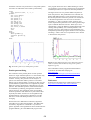
1
COMMISSION ON POWDER DIFFRACTION INTERNATIONAL UNION OF CRYSTALLOGRAPHY http://www.iucr.org/iucr-top/iucr/cpd.html NEWSLETTER No. 32, December 2005 http://www.fkf.mpg.de/cpd/html/newsletter.html IN THIS ISSUE 2D Powder Diffraction (Robert Dinnebier, Editor) CPD Chairman’s message, Bill David 2 Editor’s message, Robert Dinnebier 2 WWW sites related to Powder Diffraction 3 IUCr Commission on Powder Diffraction 3 Workshop Report: “Watching the Action” 4 2D Powder Diffraction: In situ powder diffraction – Electric Fields H. Ehrenberg 7 Datasqueeze: A Software Tool for Powder and Small-Angle X-Ray Diffraction Analysis Paul A. Heiney 9 How to add a molecule to a crystallographic surface using SCHAKAL 99 Egbert Keller 41 Discussion of the Indexing algorithms within TOPAS 43 Alan Coelho, Arnt Kern Structural phase transitions made easy: the new ISODISPLACE software tool 45 Branton J. Campbell, Harold T. Stokes, David Tanner, and Dorian M. Hatch, Derivative Difference Minimization (DDM) Program Leonid A. Solovyov 47 Density Measurement Using the Berman Balance Richard J. Staples 48 Powder3D: A Software for tailored for in situ powder diffraction studies Bernd Hinrichsen, Robert E. Dinnebier; and Martin Jansen 12 Two2One - Software for the analysis of twodimensional diffraction data Sven C. Vogel AAND Karsten Knorr 2 Fitting of nano particle structures to powder diffraction pattern using DISCUS 49 R.B. Neder1 and T. Proffen2 23 Diamond – Investigation and Visualization of Structural Changes H. Putz, K. Brandenburg 26 Magnetic Rietveld and single crystal refinement with SARAh- Representational Analysis and SARAh-Refine for the MS-Windows 51 Andrew S. Wills Detection of Ellipses in Powder Diffraction Patterns using Hough Transformation 27 Rajiv Paneerselvam, Bernd Hinrichsen, Manfred Joswig, and Robert E. Dinnebier Prediction of not-yet-synthesized phases at high and low pressures and the transitions among them using global exploration methods and ab initio calculations J. C. Schön, Z. Cancarevic, and M. Jansen Computer Corner, L M D Cranswick 31 38 New Time-of-Flight Neutron Total Scattering Data Analysis Software at IPNS 39 J. Taoa , T. G. Worltona, J. Hammondsa, C. J. Benmorea, D. Mikkelson , R. Mikkelsonb New Features of the BGMN Rietveld program J. Bergmann1, R. Kleeberg2 ISSN 1591-9552 40 Quantitative Rietveld analysis in batch mode with Maud, and new features in Maud 2.037 Luca Lutterotti Update of the FullProf Suite and CrysFML Juan Rodríguez-Carvajal 53 55 FOX, Free Objects for Xtallography version 1.7 (november 2005) Vincent Favre-Nicolin & Radovan Černý 57 VENUS: a 3D Visualization System for Crystal Structures and Electron/Nuclear Densities Fujio Izumi & Ruben A. Dilanian 59 News from the ICDD 66 What’s On 67 How to receive the CPD Newsletter 67 Calls for contributions to CPD Newsletter 33 67 CPD Chairman’s Message It is my privilege and pleasure, as the incoming chair of the Commission on Powder Diffraction, to write the introduction to this newsletter edited by the outgoing chair, Robert Dinnebier. The CPD was founded almost 20 years ago in 1987 and had its first meeting as a satellite to the main IUCr congress in Perth, Australia in that year. It is interesting to review progress over the past twenty years within the context of the reasons cited for the establishment of the CPD. "One of the most fundamental arguments for the formation of the commission was the unique position of international research using powder diffraction as its main technique. In almost all cases in the field of crystallography there is considerably more activity in published material from academic institutions than from industry. This position is exactly reversed in the field of powder diffraction and it is one of the major purposes of the commission to provide an information link between the very large industrial community and the more academic, less applied aspects of the subject." I would like to think that the boundaries between industry and academia have blurred a little over the past 20 years. Many of the most important advances have been pioneered by industry and particularly by the diffractometer companies. Faced with the phenomenal capabilities of powder diffractometers at synchrotron sources, these companies have risen to the challenge and developed machines that are able to tackle some of the most challenging topics in powder diffraction today. You will, for example, find seminal contributions from both academic and industrial researchers in this newsletter. On the other hand, academics have been able to focus more on the crystallography of real materials that are of importance to industrial sectors ranging from pharmaceuticals to energy and the environment. These are exciting times for powder diffraction and we can expect to see significant growth over the next few years. This newsletter gives a glimpse of some of the challenges that lie ahead of us. It is also my privilege and pleasure to thank the outgoing members of the Commission for their participation over their terms of office; they are Rob Delhez, Cam Hubbard, Davor Balzar and Gert Kruger - many thanks! You will find the list of current CPD members on the next page of this newsletter. I am pleased to welcome Simon Billinge, David Rafaja, Rosanna Rizzi, Peter Stephens and Pam Whitfield as new members. Do feel free to e-mail us with your thoughts and suggestions! Finally, I would like to thank Robert Dinnebier, the outgoing Chair of the Commission, for his immense energy and great dedication in fulfilling the varied roles of newsletter editor, workshop organiser, general CPD fund raiser and passionate advocate of powder diffraction. His three years as CPD chair have witnessed a dramatic development in the technique. I believe that the trend is set to continue - we have an exciting triennium ahead of us. Watch the action! Bill David CPD projects RIETVELD REFINEMENT OF ORGANIC STRUCTURES Increasing numbers of organic crystal structures are being solved and refined from powder diffraction data. The basic arrangement of the molecules in the structure can often be determined by direct methods, or by direct-space approaches. However, experience shows that problems can arise in the subsequent Rietveld refinement. For example, unless restrained by appropriate bond distances and angles molecules can distort unrealistically from a reasonable molecular structure. So how good are these Rietveld refinements? Is the problem a fundamental one of powder diffraction? eg. the ambiguities and correlations caused by peak overlap or defining the background etc. lead to inaccurate structures. Or can some of the blame be attributed to poor refinement practice? We plan to put onto the CPD web site a number of good quality powder diffraction patterns from organic compounds of known crystal structure and of different complexity. These can be downloaded, and powder crystallographers can try out their own prowess at Rietveld refinement, by comparing their refined structures with the accepted singlecrystal structures. This should be a learning exercise for us all. Any suggestions as to compounds that would appear particularly appropriate for this project are very welcome. Please contact the CPD chairman. TEXTBOOK ON POWDER DIFFRACTION R. Dinnebier and S. Billinge are editing a textbook targeted at graduate students to be published by the Royal Society of Chemistry. 2/3rd of the contributions have been received. The final deadline has been extended to early 2006. From the Editor of Newsletter 32 2D POWDER DIFFRACTION As one of my last duties as leaving chairman, it is my pleasure to edit this last issue of our CPD newsletter for the triennium 2002-2005. Powder Diffraction is an active field of research and it is exciting to watch new developments becoming routine. This is in particular true for in-situ powder diffraction employing fast 2-dimensional detectors, which is also the main topic of this newsletter. Before a exciting new technique really becomes routine, a lot of hardware and software development in combination with teaching is required. As an example, in order to handle hundreds or even thousands of high resolution powder diffraction patterns simultaneously, new generally available software must be developed and debugged. Hands on workshops are required, which not only reflect the state of the art but also teach students how to handle challenging problems. One of these workshops called “Watching the Action: Powder Diffraction at non-ambient conditions” was recently held at the MPI in Stuttgart. In order to make the proceeding to this workshop available to a broader readership, I decided to incorporate the full papers into the newsletter, which explains the slight “oversize” of this issue. Supplementary material, additional tutorials and many abstracts can also be found at http://www.fkf.mpg.de/xray. Robert Dinnebier 2 WWW sites related to powder diffraction The Commission on Powder Diffraction (CPD): http://www.iucr.org/iucr-top/iucr/cpd.html The International Union of Crystallography (IUCr): http://www.iucr.org/ The International Centre for Diffraction Data (ICDD): http://www.icdd.com/ The International X-ray Analysis Society (IXAS): http://www.ixas.org/ CCP 14: http://www.ccp14.ac.uk/ Submitting a proposal for neutron diffraction or synchrotron radiation X-ray diffraction is possible at many (publicly funded) large scale facilities in the world. It represents an important and frequently unique opportunity for powder diffraction experiments. A useful guide and information can be accessed through the following web-site, maintained by R. Dinnebier at http://www.fkf.mpg.de/xray This list is far from being complete and needs input from users and readers of the CPD Newsletter. Please send comments to R. Dinnebier ([email protected]) THE IUCR COMMISSION ON POWDER DIFFRACTION - TRIENNIUM 2005-2008 Prof. Dr. D. Rafaja (David) Institute of Physical Metallurgy, TU Bergakademie Freiberg, Gustav-Zeuner-Str.5 D-09599 Freiberg, Germany e-mail: [email protected] Telephone: +49(3731)392299 | Fax: +49(3731)393657 e-mail: [email protected] home: www.tu-freiberg.de/mk/ Chairman: Prof. W. I. F. David (Bill) Rutherford Appleton Laboratory (CCLRC), Chilton, Oxon. OX11 OQX, United Kingdom Telephone: +44 1235 445179 | Fax: +44 1235 445643 e-mail: [email protected] Secretary: Prof. A. N. Fitch (Andy) ESRF, BP220, F-38043 Grenoble Cedex, France Telephone : +33 476 88 25 32 | Fax: +33 476 88 25 42 e-mail: [email protected] Dr. R. Rizzi (Rosanna) CNR IC - c/o Dip. GeomineralogicoVia Orabona 4, Bari, I-70125 , Italy (map) Telephone: 39(80)5442624 | Fax: 39(80)5442591 e-mail: [email protected] Prof. Dr S. Billinge (Simon) Department of Physics and Astronomy 4268 Biomed. Phys. Sciences Building Michigan State University East Lansing, MI 48824 Telephone:+1-517-355-9200 x2202 | Fax: +1-517-353-4500 email: [email protected] home: http://www.totalscattering.org/ Prof. Dr. P. W. Stephens (Peter) Peter W. Stephens, Professor Department of Physics & Astronomy State University of New York Stony Brook, NY 11794-3800, USA Telephone: +1 (631) 632-8156 | Fax: +1 (631) 632-4977 e-mail: [email protected] home: powder.physics.sunysb.edu Prof. M. Delgado (Miguel) Laboratorio de Cristalografía, Departamento de Química, Facultad de Ciencias, La Hechicera. Universidad de Los Andes, Mérida 5101 Venezuela. Telephone: +58 274 240 13 72 e-mail: [email protected] Dr Pamela Whitfield (Pam) CChem MRSC Energy Materials Institute for Chemical Process and Environmental Technology, Building M12 National Research Council Canada 1200 Montreal Road, Ottawa ON K1A 0R6, CANADA Telephone: (613) 998 8462 | Fax: (613) 991 2384 Email: [email protected] home: http://icpet-itpce.nrc-cnrc.gc.ca/ Dr. I. Madsen (Ian) CSIRO Minerals Box 312, Clayton South 3169 Victoria, Australia Telephone: +61 3 9545 8785 | Fax: +61 3 9562 8919 e-mail; [email protected] Prof. N. Masciocchi (Norberto) Dipartimento di Scienze Chimiche e Ambientali, Università dell'Insubria, via Valleggio 11, 22100 Como (Italy) Telephone: +39-031-326227 | Fax: +39-031-2386119 [email protected] http://scienze-como.uninsubria.it/masciocchi/ ICDD Representative Prof. R. L. Snyder (Bob) Department of Materials Science & Engineering, Georgia Institute of Technology, Columbus, 771 Ferst Dr. N.W., Atlanta, GA 30332-0245, USA; Telephone: +1 (404) 894-2888 | Fax: +1 (404) 894-2888 e-mail: [email protected] 3 Dr. J. A. Kaduk (Jim) BP Chemicals, 150 W. Warrenville Rd., P.O. Box 3011 MC F-9, Naperville, IL, 60566, USA Telephone: +1(630)4204547 | Fax: +1(630)4205252 e-mail: [email protected] Consultants: Dr James Cline (Jim) Ceramics Division, National Insititute of Standards and Technology, 100 Bureau Dr Stop 8523, Gaithersburg, Maryland, 20899, USA e-mail:[email protected] Dr. Irene Margiolaki ESRF, BP220, F-38043 Grenoble Cedex, France Telephone : +33 476 88 21 48 | Fax: +33 476 88 29 07 e-mail: [email protected] Dr Johan Pieter Roos De Villiers Mineralogy Division, MINTEK, Private Bag X3015, Randburg, 2125, South Africa Telephone: +27(11)7094745 | Fax: +27(11)7094564 e-mail: [email protected], [email protected] Prof. P. Scardi (Paolo) Dipartimento di Ingegneria dei Materiali e Tecnologie Industriali, Università di Trento, 38050 Mesiano (TN), Italy; Telephone: +39 0461 882417/67 | Fax: +39 (461) 881977 e-mail: [email protected] Dr R. E. Dinnebier (Robert) Max-Planck-Institut für Festkörperforschung, Heisenbergstrasse 1, D-70569 Stuttgart, Germany Telephone: +49-711-689-1503 | Fax: +49-711-689-1502 e-mail: [email protected] home: www.fkf.mpg.de/xray Dr. M. Yashima Tokyo Inst. of Technology, Grad School of Sci. & Engn. Dpt. of Matls. Sci.& Engn. Nagatsuta-cho 4259-J1-4 Midori-ku Yokohama, 226-8502, Japan e-mail: [email protected] The evening program consisted of a wine tasting of selected German produce. A delicious buffet dinner complemented the wines, all hand picked by Robert Dinnebier, perfectly. This social event was only possible due to the friendly support of our industrial sponsors. Workshop Report “Watching the Action” An international workshop on in situ powder diffraction organized by Robert E. Dinnebier, Bernd Hinrichsen and Martin Jansen was held in Stuttgart in the first week of October. The Max-Planck-Institute for Solid State Research hosted the event spanning two days, organized under the auspices of the DGK, CPD and MPG. Various aspects of this fascinating experimental method were presented during the morning sessions, the afternoons being reserved for ‘hands-on‘ tutorials in data reduction, presentation and Rietveld refinement. Twelve participants contributed short presentations, detailing their current research in the field and also presenting experimental facilities. The opening presentation by Paul Norby went directly to the heart of the matter, giving insight into novel high speed synchrotron experiments aimed at studying chemical reactions. Christian Schoen showed us what we are looking for in his talk on structure prediction of new high and low pressure phases. After the coffee break image analysis filled the rest of the morning session. Some general aspects of image filtering techniques were introduced by Manfred Joswig. Bernd Hinrichsen presented a real application of some of these techniques within the novel image plate integration software Powder3D-IP. Arndt Kern focused on laboratory experiments, giving a detailed view of the challenges facing the experimentalist during high temperature experiments. He wowed the crowd with some novel applications of the Rietveld refinement software Topas. The remaining working day was spent practicing data reduction and presentation using the software Powder3D (http://www.fkf.mpg.de/xray). The next day started with as much fervour as the previous had ended. Ulrich Schwarz teaching us the intricacies of high pressure powder diffraction experiments. Gaining a better understanding of batteries motivates the electrical field in situ studies of Holger Ehrenberg. His presentation of the Hasylab beamline B2 dedicated to in situ experiments proved the high level of dedication and specialization in the field. Holger Putz presented the powerful capabilities of Diamond when visualizing structural changes. The capability to create films easily being responsible for the greatest interest. The rest of the day was spent following the incomparable Juan Rodriguez-Carvajal during his presentation and tutorial of Fullprof. The cyclic mode making structural analysis of large in situ data collections much more manageable. Late Friday afternoon saw the last of the ninety participants leave for home, weighed down by the workshop manuscript but certainly inspired to take up the in situ challenge. The organizers would like to thank the DGK for the generous financial support of the event, this allowed the registration fees to be waived. The workshop manual and some impressions are available online under http://www.fkf.mpg.de/xray. 4 – S N O I T U L ES O G S N E N L L O I A CH ACT R L F A F I C I D T Y 8 D ANAL y R U O Y in all X-ra s E s e r G g A o r p MAN tectors ntinual ndling, de nds for co IONS sta ample ha for higher data s T , U s L c ti O p S o ay ACTION novations urces, X-r in o s o y w T a D8 DIFFR r . X m r o s: nologies: mon platf the D8 capabilitie m o c a core tech n o enhance are – all and softw ample throughput ds es quality an ple batch m a s e g r tervention la r in r fo e r s e n u g t n u Cha conversio t ge witho u a o s h u Auto it t n w e ns um vestigatio ctive instr in n io s Effe is m and trans n o ti c e fl e tors R TM near detec urements s li a e m 1 r C te fas TM nd VÅNTE a rding of 50 times o 1 c e r e y r fo E t x e o n g y h ra -S L heta cove ond Snap T c e 2 s ° 1 3 r e fo g ge Lar ta covera e h T 2 ° 2 e1 Hug processes c ti a m e kin BRUKER ADVANCED X-RAY SOLUTIONS www.bruker-axs.com 5 D8 ADVANCE Auto Changer LynxEye.1 1 02.12.2005 12:53:34 ANOTHER FIRST FROM PANALYTICAL! New X’Pert PRO for transmission allows for diffraction measurements on proteins Le Bail fitting Profile function: Pseudo Voigt Asymmetry correction: Finger-Cox-Jephcoat Cell parameters: a=78.99 Å c=37.87 Å Indexing was carried out using X’Pert HighScore Plus software. Further processing using Le Bail fitting method provided excellent agreement with the cell parameters achieved by single crystal diffraction. Using PANalytical’s new transmission geometry with PreFIX focusing mirror, in conjunction with the X’Celerator detector, diffraction experiments on macromolecules such as proteins can now be carried out with an X’Pert PRO MPD X-ray diffraction system. Characterized by weak scattering and small sample volumes, these materials have previously been considered ‘difficult’ for X-ray diffraction. Instead, protein structure determination traditionally relied on the use of single crystal systems, or beam lines for the extraction of powder patterns. Here, we show for the first time that protein powder data measured on a laboratory X-ray diffraction system can be used for crystallographic analysis. The X’Pert PRO MPD fitted with the focusing mirror, capillary spinner and X’Celerator detector Emphasis on the research and development of macromolecules – especially in areas such as protein pharmaceutics – has increased strongly in recent years. By offering researchers the potential for pre-screening and investigation of protein-based medicines within the laboratory, use of the transmission setup represents a significant technical advance. As a PreFIX optic, the focusing mirror is interchangeable with all other available incident optics for the X’Pert PRO MPD without the need for any re-alignment. From a technical perspective, it means: • the size of the capillary tube no longer governs resolution • peaks narrower than 0.05 degrees are easily resolved. Use of the X’Celerator detector, meanwhile, ensures fast data collection. Transmission experiments on hen egg white lysozyme using an X’Pert PRO MPD fitted with the new mirror and the X’Celerator detector, provided high resolution data sufficient to enable cell searching, indexing and unit cell refinement. The lattice parameters determined were in good agreement with literature data obtained from single crystal measurements. To find more about PANalytical’s X’Pert PRO for transmission, contact PANalytical. Acknowledgement: We thank Dr. B. Prugovečki, University of Zagreb, Croatia for the lysozyme crystallization, sample preparation of capillary and stimulating discussions. The Analytical X-ray Company PANalytical B.V. P.O. Box 13 7600 AA Almelo The Netherlands t: +31 546 534444 f: +31 546 534598 e: [email protected] www.panalytical.com 6 in situ powder diffraction – Electric Fields H. Ehrenberg Materials Science, Darmstadt University of Technology, Petersenstr. 23, D-64287 Darmstadt The investigation of materials under real operation conditions is of primary importance for materials science. From a more basic research point of view the underlying working principles can be elucidated, guiding the route to advanced functionalized materials. On the other hand, degradation mechanisms can also be revealed, allowing a goal-aimed optimization of cycle stability in long-time operation by minimizing fatigue. Two main challenges for such studies can be summarized: 1. "Materials" are normally multi-phase components, combined in a specific way to form highly inhomogeneous devices, far away from ideal crystal structures. 2. "in situ" conditions require sample environments, which restrict the observations either by additional disturbing signals or "hide" the object of interest by not-transparent shieldings. A promising approach to in situ materials characterisation has to follow three steps: (i) identification of a suitable probe, (ii) design of an operating test cell, (iii) combination with an adapted dector system. For structural studies of polycrystalline materials under operation the use of synchrotron radiation can overcome most of the limitations: High-energetic radiation (short wavelength) has a very good penetration capability, the high intensity allows fast data collection with good time resolution, and the low vertical divergence can reveal also subtle details by the small (and in most cases neglectable) instrumental contribution to the observed reflection profiles in powder diffraction. In this contribution two examples for the characterisation of materials, driven in operation by electric fields, are shown: 1. Piezoelectric Pb(Zr,Ti)O3 ceramics are polarized by electric fields, and the resulting strain is used in actuators. 2. Li(Co,Ni)O2 allows to extract and reinsert Li-ions. This reversible process is exploited in the cathode of rechargeable Li-ion batteries. During charging the electric field of the external charger pumps electrons from the cathode to the anode and induces, for charge compensation, a movement of one Li+-ion per electron from the cathode to the anode through a Li-conducting, but for electrons insulating electrolyte. 7 30000 (101) 0 kV/mm 5.5 kV/mm 20000 (110) 10000 0 The pictures show a PZT ceramic with sputtered Ptelectrodes as used in the in situ device (left) and the whole device mounted on the diffractometer B2 [1] at HASYLAB (middle). The position-sensitive detector OBI [2] can also be seen and covers the whole 2θ range simultaneously. For more information on the specific sample see reference [3]. A section of two diffraction patterns (λ = 0.49975 Å) is shown on the right hand side for different states of poling. The effects of microstructural changes are clearly reflected in the different profiles. The evolution of these profiles along hystereses loops is reversible and has to be correlated with the underlying microstructure; these analyses are still in progress [4]. Two different test cells for in situ studies of the electrochemical Li-extraction and -insertion have been developed [5,6]: However, differently prepared LiMn2O4 samples show a very distinct behaviour. All three phases are of spinel-type structure and differ probably in the cation distribution on the tetrahedral and octahedral interstitials. The in situ technique allows to follow structural changes during operation and does not suffer from relaxations or reactions, which might occur before ex situ studies after dismounting of a battery. The test cell is further improved at present with respect to life-time stability. At least 100 charge-discharge cycles are needed to investigate fatigue in the cathode. SwagelokTM housing Al Cu Cathode mix Beam Sealings The following figure shows the complete diffraction pattern for LiMn2O4 as observed before charging and calculated by the Rietveld method using the program package Winplotr [7]. Note that phase-specific sample shifts from the diffractometer centre have to be taken into account, because of the sequential arrangement of Al-current collector, cathode and Li-anode along the beam direction. The newer versions of Fullprof can handle this important feature. Financial support from the Helmholtz Association of National Research Centres (Virtual Institute VH-VI102) for the "development of dedicated in situ environments for the characterisation of polycrystalline materials using high-energetic synchrotron radiation" is gratefully acknowledged. Electrical fatigue in functional materials is investigated in the λ = 0.69956 Å frame of the DFG Collaborative Research Centre SFB 595. Experiments and analyses on PZT ceramics are performed by K. A. Schönau, M. Knapp and H. Fueß, on Li-ion battery materials by N. N. Bramnik, K. Nikolowski and C. Bähtz. (111) 52000 39000 (311) 26000 Al 13000 0 19 7 43 2θ/° The changes of diffraction patterns during charging and discharging are already described in detail [5]. During charging and discharging the original phase A with maximum Li-content disappears and two other phases B and C with smaller lattice parameters are formed conteracting, see next figure. For this sample, prepared by sub-solidus reaction, a three-phase mechanism of Li-extraction and reinsertion was established. Phase 100% A B C 0% 8.34 charge A discharge a/Å B 8.24 C This method was also successfully applied to other cathode materials: Li(Co,Ni)O2 [8,9], Li(Mn,Fe)PO4 [10] and LiCoPO4 [11]. xmax xmin 8.14 8 [1] M. Knapp, C. Baehtz, H. Ehrenberg, H. Fuess, J. Synchrotron Rad. 11 (2004) 328334. [2] M. Knapp, V. Joco, C. Baehtz, H. H. Brecht, A. Berghaeuser, H. Ehrenberg, H. 55 von Seggern, H. Fuess, Nucl. Instrum. Meth. A 521 (2004) 565-570. [3] K. A. Schönau, M. Knapp, N. Balke, H. Ehrenberg, H. Fuess, Z. Kristallogr. Suppl. 22 (2005) 127. [4] K. A. Schönau, PhD Thesis, Materials Science, Darmstadt University of Technology. [5] C. Baehtz, Th. Buhrmester, N. N. 55 Bramnik, K. Nikolowski, H. Ehrenberg, Solid State Ionics 176 (2005) 1647-1652. [6] K. Nikolowski, C. Baehtz, N. N. Bramnik, H. Ehrenberg, J. Appl. Cryst. 38 (2005) 851-853. [7] T. Roisnel, J. Rodriguez-Carvajal, Mater. Sci. Forum 378-381 (2001) 118123. [8] T. Gross, T. Buhrmester, K. G. Bramnik, N. N. Bramnik, K. Nikolowski, C. Baehtz, H. Ehrenberg, H. Fuess, Solid State Ionics 176 (2005) 1193-1199. [9] H. Ehrenberg, K. Nikolowski, N. N. Bramnik, C. Baehtz, T. Buhrmester, T. Gross, Adv. Eng. Mater., in print. [10] N. N. Bramnik, K. G. Bramnik, K. Nikolowski, M. Hinterstein, H. Ehrenberg, Electrochem. Solid-State Lett. 8 (2005) A379-A381. [11] N. N. Bramnik, K. G. Bramnik, C. Baehtz, H. Ehrenberg, J. Power Sources 145 (2005) 74-81. Datasqueeze: A Software Tool for Powder and Small-Angle X-Ray Diffraction Analysis Paul A. Heiney Department of Physics and Astronomy University of Pennsylvania 209 S. 33rd St. Philadelphia, PA 19104, U.S.A. [email protected] Figure 1. Schematic of a typical XRD experiment employing an area detector. Introduction A substantial portion of X-ray Diffraction (XRD) research is today performed using two-dimensional (2D) positional detectors, also known as area detectors. Such detectors measure the scattered intensity over a surface, and save the data as an array of pixel intensities. The researcher must then interpret this array of intensities to obtain a structural model for the system of interest. Typically, the detector manufacturer supplies software for reading the obtained data files and performing some kind of primary data processing. However, this software varies in quality, and even when it is well designed it may not suit the needs of the user. For example, the scientist may be performing small-angle x-ray scattering (SAXS) using an instrument that the manufacturer had intended for use with singlecrystal structure refinement. The hardware itself could be perfectly adequate for the purpose, but the manufacturer’s software ineffective at extracting the kind of information desired. Furthermore, the supplied software often runs only on the computer used for collecting the data. The scientist may have obtained the data at a central facility or synchrotron, and wish to analyze the data back at his or her own desk. Here we describe a software application, Datasqueeze [1], that can be used to analyze data from a wide variety of xray area detectors. Datasqueeze runs on Windows, Linux, and Macintosh OS X. It is particularly useful for the analysis of powder diffraction data, diffuse scattering from polymers or liquid crystals, or small-angle scattering from colloids, polymers, or gel solutions. (Datasqueeze is not well suited for analysis of single-crystal diffraction patterns with many sharp Bragg peaks). This article discusses the capabilities of Datasqueeze, and also reviews some common problems and concerns encountered when analyzing data from area detectors. X-ray Detector Properties Figure 1 shows a schematic of a typical XRD experiment using an area detector. The incident beam, which is monochromatic (with wavelength λ) and collimated, strikes a sample. The transmitted beam is blocked by a beamstop, to avoid damaging the detector. The scattered radiation strikes the detector. The detector records the integrated intensity in each pixel, but the quantity of interest is generally the scattered intensity measured as a function of 2θ (the angle between the primary beam and the scattered beam) and χ (the orientation on the detector relative to an arbitrarily chosen direction). The scattering angle is often characterized using the momentum transfer q=(4π/λ) sin θ, which can also be represented using Cartesian coordinates qx=q cos χ, qy=q sin χ. 9 Depending on the experiment being performed, the user will wish to extract different information. In a typical SAXS or powder diffraction experiment, the quantity of interest is the radial dependence of the intensity, I(q), integrated over all χ. If the sample is a fiber or liquid crystal, the user may wish to obtain I(q) profiles evaluated at different values of χ. If the material is a partially oriented polymer or poorly ordered crystal, the quantity of interest may be the “mosaic,” obtained by plotting I(χ) at a chosen value of q (this is sometimes known as a “pole figure”). The most commonly employed detector technologies are image plates, gas (wire) detectors, and charge-coupled device (CCD) cameras. Each has its advantages and disadvantages. Image plates are often the least expensive. They offer high dynamic range in intensity, but the duty cycle can be low due to the time required to read the data and prepare the plate for the next image. Wire detectors (in which crossed wires are embedded in an ionizable gas) offer fast readout and very low background noise, but can only support relatively low count rates; they are commonly employed in laboratory settings (fixed tube or rotatinganode generators). CCD detectors are the most expensive. They do not have a count rate limitation, but tend to have a fairly high readout noise (on the order of tens of counts per pixel); they are most often used in synchrotron applications. From the user’s point of view, however, the data from all three detector types, once obtained, look quite similar: an array of pixel intensities, generally in a file format unique to the manufacturer of that detector. In the analysis of XRD images, considerable attention is often paid to questions of instrumental resolution: how does the width of a diffraction peak depend on the physical size and divergence of the incident beam, the sample size, the sample-detector distance, the pixel-by-pixel resolution of the detector, etc. Less attention is sometimes paid to the angular linearity of the detector itself. In wire detectors, for example, the positions of the wires within the detector may very from nominal values, and “parallax” corrections of the photon path through the detector can be substantial. In our experience, this can lead to discrepancies between measured and calculated peak positions on the order of |∆q/ q |~2-4%, even after linearity corrections are applied by the data gathering program. Similarly, CCD detectors generally consist of a fluorescent screen, focusing optics, and the actual CCD detection plate. Distortion by the focusing optics can induce nonlinearities in measured peak positions; the quality of these optics is one of the primary differences between expensive and very expensive X-ray CCD cameras! Data from image plates can also suffer from distortions caused by waviness in the collecting plate or irregularities in the scanning hardware. Data Input Most commonly, the scientist will be analyzing a single data set at a time, but sometimes they are combined. One common situation is where many frames are collected under the same conditions. Datasqueeze can add up to eleven such files to produce a single composite dataset, while keeping track of counting statistics, etc. A somewhat more complicated situation is encountered when the user has collected a background data set, for example air scattering with no sample in place. Under these circumstances, the natural tendency is to perform a one-toone subtraction of the background data from the sample data, but this is almost always incorrect. It is important to understand all the possible sources of background. There may be a constant, source of “readout” noise, as discussed above in the case of CCD detectors. This should clearly just be subtracted from each data file, independent of count time. There may be background scattering that originates from the primary beam after it passes through the sample. This scattering will be proportional to the integration time but also depend on how much the primary beam was attenuated by the sample. Background originating upstream of the sample, on the other hand, will not be affected by sample attenuation. Datasqueeze can accomplish all of these manipulations (i.e., addition or subtraction of a constant term, subtraction of a background file multiplied by a scaling term depending on the sample attenuation), but it is important for the user to clearly understand the source of the background scattering rather than simply blindly subtracting a “background file.” neighbors. Similarly, if a pattern is very noisy, due to low signal (poor counting statistics), blocks of pixels can be binned together to produce an image with lower resolution but less noise. Calibration In order to quantitatively interpret an x-ray scattering pattern, it is necessary to map detector pixels to scattering angle units (q/χ or qx/qy). To accomplish this, the following instrumental parameters must be known with some precision: the wavelength λ, the pixel coordinates (xc, yc) of the beam center, the angular span of the detector as seen from the sample, and the orientation of the detector relative to the primary beam. The wavelength must be independently obtained; it cannot be inferred from the data. Since there is usually a dark patch in the image due to the beam stop, it is tempting to assign (xc, yc) to the geometric center of the beam stop image, but this is almost always wrong; the beam center usually differs from the beam stop center by a few pixels, and misidentification of the (xc, yc) by even a fraction of a pixel can have significant consequences. Instead, by measuring a calibration sample such as silver stereate, silver behenate, LaB6, or silicon, one obtains a powder diffraction pattern consisting of a set of concentric Bragg rings. The instrumental parameters can then be calibrated by requiring that (xc, yc) be at the center of the rings, the scattering angles of the rings correspond to known d-spacings, and that the rings be circular after correcting for possible detector misorientation relative to the primary beam. Data Display and Processing The scientist generally wants to visualize the data before performing quantitative analysis. Datasqueeze presents the data as a false color image, with tunable maximum, minimum, and contrast. To locate features of interest, a polar or Cartesian grid can be superimposed on the data, as shown in Figure 2. Figure 2: False color image of a fiber diffraction pattern, showing superimposed qx-qy Cartesian grid. Data collected at the University of Pennsylvania [2]. Note that, because the scattering plane is not identical to a reciprocal space plane (the Ewald sphere is projected onto a plane), the constant-qx -qy or curves are not straight lines. Further manipulations can be performed at this stage. Data from CCD cameras often contain isolated bad pixels, arising from electronic noise; the “dezing” feature searches for pixels that are astatistically different from their neighbors and replaces them with the average of their 10 Figure 3: Calibration using AgBe standard. (a) The calculated rings (dashed curves) do not match the measured rings (red and yellow). (b) After optimization, the two sets of rings overlap. Datasqueeze provides three methods for accomplishing this calibration. First, if the calibration parameters are already known for a particular data set, the user can simply type them in. Second, the measured diffraction pattern can be visually compared with the predicted d-spacings, and the detector parameters optimized to make them overlap, as shown in Figure 3. Finally, program can automatically refine detector parameters using a user-selected Bragg ring. Data Reduction After the data set is properly calibrated, one often wishes to collapse the 2D pixel array (typically 106-107 pixels) to a one-dimensional x-y list of intensities, consisting of 102-103 items. As discussed above, this might consist of I(q) integrated over all χ for a powder diffraction measurement, I(q) integrated over a limited range of χ for a fiber measurement, I(χ) integrated over a finite range of q for a pole plot figure, I(qx) integrated over a finite range of qy values, etc. Datasqueeze provides a variety of plotting option, and in each case the user can either input the desired range and plot increment directly, or graphically select the range using the false color image. Summary Datasqueeze is a powerful tool for the analysis of 2D X-ray diffraction patterns, especially those arising from smallangle or powder diffraction. In addition to the features described above, it provides facilities for pixel-by-pixel examination of the data, extraction of statistics regarding distributions of intensities among pixels, and indexing of simple powder diffraction patterns using a graphical interface. In addition to the graphical interface, the program can run in a “batch” mode for automated processing of many files. A particular strength of the program is that it is still evolving. A new version is released every 2-4 months, generally incorporating improvements or new features suggested by users. Anticipated upgrades to the program include support for yet more data formats, more options for 2D to 1D data reduction, and improved support for nonEnglish speaking readers. References [1] The description of Datasqueeze in this article does not constitute or imply an endorsement by the University of Pennsylvania. Datasqueeze can be obtained from http://datasqueezesoftware.com. A manual with more detailed information on the program is available as a free download from the same site. [2] The instrumentation is described at http://www.lrsm.upenn.edu/lrsm/facMAXS.html [3] D. W. Marquardt, J. Soc. Ind. Appl. Math. II, 2, 431441 (1963)). Figure 4: (b) Shows the radial I(q) plot (equivalent to a θ2 θ plot) showing the intensity profile of the bright ring on right in the fiber pattern in (a). Data were averaged over the range χ=±20º. Red dots show the extracted data; solid curve shows the results of a least-squares fit. Lower panel in (b) shows fit residuals (i.e., [[model-data]/error] 2). Once extracted, the x-y data can be graphed, saved for future analysis, or compared via a least-squares-fit analysis to a variety of commonly used functional forms (Lorentzian and Gaussian peaks, power law, Rayleigh and Bessel functions, etc.). Least-squares fit aficionados are provided with detailed information on multi-parameter error bars, correlation coefficients. etc. Figure 4 shows a radial plot through the bright ring on the right-hand side of the fiber pattern shown in Figure 2. The data have been leastsquares fit to a sum of three Lorentzian functions and a linear background, using the Marquard nonlinear leastsquares minimization algorithm [3]. 11 Powder3D: A Software for tailored for in situ powder diffraction studies Bernd Hinrichsen, Robert E. Dinnebier and Martin Jansen Max Planck Institute for Solid State Research, Heisenbergstrasse 1., Stuttgart Introduction Powder3D is a program for data reduction and publication quality visualisation aimed specifically at large data sets collected in time resolved powder diffraction experiments. The program is in ongoing development, so there shall be regular updates and extensions to the present functionality. For comments or suggestions please contact [email protected] . Getting Started Installation The latest version of Powder3D can be downloaded from http://www.fkf.mpg.de/xray. As Powder3D is written in the programming language IDLTM you will need to install the IDL virtual machine (IDL VMTM) before being able to run Powder3D. Virtual machines for various platforms can be downloaded from the RSI website http://www.rsinc.com/idlvm/ free of charge. When you have installed IDL VMTM unpack Powder3D into a directory of your choice and double click on the file ‘Powder3D.sav’. After dismissing the IDL VMTM (current version 6.1 only) splash screen the following window (Figure 1) should welcome you. Please note: the libraries necessary for the AVI export and peak refinement, namely ‘IDLtoAVI.dll’, ‘IDLtoAVI.dlm’, ‘p3d.dlm’ and ‘p3d.dll’ should be in the same directory as Powder3D. The functions only work on the Windows® operating system. Other operating systems are not supported. UNC (unmapped network) paths will cause the program to fail. Figure 1. : Welcome screen Table 1: Phases identified in the sample data set Phase SG a/Å b/Å c/Å Pbam 11,29 6,29 3,62 δRb2[C2O4] γ6,33 10,45 8,22 P21/c Rb2[C2O4] βPnma 8,16 6,58 10,9 Rb2[C2O4] P63/m α6,47 8,26 Rb2[C2O4] mc α5,89 7,80 P63/m Rb2[CO3] mc Pnma 7,68 5,89 10,14 βRb2[CO3] γ5,87 10,13 7,31 P21/c Rb2[CO3] β/° 98,0 2 97,3 Range Æ 653K Æ 653K Æ 661K Æ 723K Æ 830K Æ 600K The temperature ramp was set to 298 Æ 838 Æ 298 K. The sample was heated at a rate of 2.8 Kmin-1 and cooled at a rate of 4.8 Kmin-1. Considering the exposure and development time this leads to a heating rate of 4.2 Kframe1 and a cooling rate of 7.62 Kframe-1. The sample data set The data set that is the basis for the graphics displayed in the manual is available for download from http://www.fkf.mpg.de/xray. The data stems from an experiment carried out at the X7B beamline of the NSLS (Dinnebier et al., 2005). The wavelength was 0.9224 Å. The initial substance was δ-Rb2[C2O4]. Seven phases can be identified and are tabulated below: Figure 2. : Powder diffraction patterns, lattice parameters, and cell volumes of Rb2[C2O4] and Rb2[CO3] as a function of temperature in the range from 298 to 838 K (2.4 K min-1 and back down to 298 K (4.8 K min-1). Taken from (Dinnebier et al., 2005). 12 Import One of the first things you shall want to do is to import data. To do that press the import button (Figure 3) or select ‘File’ > ‘Import’. Figure 3.: Import menu Figure 5.: Import settings Six different formats are available, although XY and Chi formats are identical. You shall be prompted to select a file (Figure 4). Standard versions of GSAS (GDA), Fullprof (DAT), Bruker (UXD) and DASH (XYE) data files are imported. After the files have been read a message displays a few details on the array (Figure 6). There is no set limit to the number of files that can be read, the only limitation is the available memory. Figure 6.: Import report As soon as you acknowledge the message you are displayed the first of your powder patterns (Figure 10). Figure 4.: Select import files Select any file of your set. Once you press open a search for all files with a suffix identical to the selected file within the given directory is started. Beware – this search is recursive, if you have further file in subdirectories matching the search pattern these shall also be loaded. The files are sorted according to the last number in the file names. A specific suffix is not necessary – Powder3D does however filter for the endings according to the selected file format in the file selection dialog. Should your files have a different suffix, type *.<your suffix here> <Enter> in the ‘File name’ field to display them. Upon pressing enter the file names in the directory are read and sorted, then the first file is loaded and the theta range read. The next window prompts you for the wavelength and the two theta range and increment. The increment entered can not be altered later. The range can only be cropped. Should the range of your files differ from the set values the intensities are interpolated using the selected function (linear, quadratic or spline). The entries correspond to the values of the sample data provided. Single pattern loading and deletion Should you wish to load a single pattern only , or wish to compare a pattern to already loaded data, this can be done by using the function, ‘Edit’ > ‘Add Pattern’ (Figure 7.). The pattern is added to the end of the pattern array. Should the pattern differ with regard to the step width or position the intensities are interpolated to match the range and step width of the data already loaded. A dialog requiring you to enter the wavelength for this pattern is displayed. If a pattern needs to be deleted, select it in the ‘2D-Plot’ window and choose ‘Delete pattern’ from the ‘Edit’ menu. Should you wish to delete any number of patterns, select them in the pattern list and select the function ‘Edit’> ‘Remove Patterns’ from the menu bar. Figure 8.: Adding a single pattern 13 Figure 12.: Cropping bars Figure 9.: Pattern selection tool On pressing the enter button the entire array is cropped to the new range. Please note: It is a good idea to save the data regularly to avoid possible data loss. (‘File’ > ‘Save’). Single pattern visualization Figure 13.: Zoom button Figure 10.: The first powder pattern Data reduction Cropping tool The limits of the powder patterns generally need to be changed. This is conveniently done by means of the cropping tool. A click on the crop button (Figure 11) draws two vertical lines, which you can drag to define the desired range (Figure 12). Figure 14.: Zoom tool The default tool in the 2D-plot window is the zoom box (Figure 14). Pull it over a region you wish to enlarge. Once the enlarged window is displayed click in the borders around the plot to navigate. A click to the right of the Xaxis moves the pattern(s) to the left and displays the pattern in a 2Θ region shifted 10% higher. Clicking in the other borders works in analogous fashion. A single click in the plot window resizes it to the maximum view. Selecting multiple patterns from the list displays them up to 6 colour coded overlaid patterns (Figure 15). Figure 11.: Crop button 14 wavelengths for some standard anode elements have integrated in the top list. Figure 17.: Wavelength dialog Figure 15.: Multiple pattern display An interesting feature is the ability to export an AVI film of the single patterns cycling through the selected sets and the zoomed range. To do this press ‘Export > AVI’ in the context menu. To make this export as versatile as possible it creates a film only of the currently selected data range ( Θ, intensity and selected data sets). You will have to select an appropriate compression algorithm for the video. In our experience DiVX4 high motion gives the best results. This feature is only available on the Windows® operating system. Please note the installation of the library for this function are described above (see Installation). Normalizing Patterns Data collected using image plates generally lacks a beam decay correction. This can be partially alleviated by a normalization. Two or more patterns can be corrected using this function (Menu Edit>Normalize patterns). Select the patterns via the list or select patterns belonging to a phase by choosing the appropriate phase. Next ensure the method of normalization is correct. All patterns that have been selected are superimposed over one another. It is possible to zoom by dragging open a zoom box with a left click. Select the region you wish to normalize the patterns with by dragging over a range with a right click. The range selected in this manner is used to normalize the data. By pressing ‘Test’ you can preview the results of the normalization. Press ‘Cancel’ to discard or ‘OK’ to accept the normalization. Figure 16.: Normalization function Phases and ranges The increments between the patterns can be entered into a table (Figure 18) which is called by ‘Edit’ > ‘Increments and phase ranges’. For unvarying increments the fields on the right of the window can be used to insert values into the table. Once two of the first three fields are filled the other is calculated and filled automatically. Should all fields contain values no updating takes place. Pressing the ‘Insert’ button fills the table with the calculated values. These values are used for labelling purposes only. Figure 18.: Insert increments Adding phase ranges can either be done manually by editing the fields of the range table (Figure 19). Please note: while editing you have to leave the cell you are editing for the values to be read properly by the ‘Insert’ command. The aid for entering the values at the bottom of the window works in the same fashion as that used in the increment window. These values are necessary for the Le Bail/Rietveld assistant of which a first version is included. Figure 19.: Define phase ranges Wavelength The wavelength dialog accessible via the menu Edit>Wavelength allows you to alter the radiation wavelength (Figure 17). Should you wish to recalculate the pattern, select the radio button ‘recalculate patterns’. The 15 Kα2 stripping Should you have collected laboratory data using Kα1 and Kα2 rays these can be separated using the menu ‘Edit’ > ‘Kalpha stripping’. Select which wavelength you wish to keep (Figure 20). Figure 22.: Smoothing window Figure 20.: Kα2 stripping The following dialog (Figure 21) enables you to select the sets, which should be stripped. The raw data is overwritten and therefore this action cannot be undone. The correct selection of the function shape has great effect on the smoothing efficacy. Background Figure 21.: Batch stripping Smoothing An advanced full width at half maximum (FWHM) optimised smoothing (Figure 22) algorithm described by Dinnebier (Dinnebier, 2003) is implemented (‘Edit’ > ‘Smoothing’). The variation of the FWHM of the peaks is generally described by the Caglioti (Caglioti et al., 1958) formula: FWHM = U tan 2 θ + V tan θ + W This can be graphically set with aid of the function window on the left. Here the function can be dragged to the desired shape with the aid of three red boxes. 16 Figure 23.: Background reduction Background determination (‘Edit’ > ‘Background’) can be done in two modes. Either a pattern can be loaded (XY format as for import) or it can be calculated (Figure 23). Should a pattern be loaded, it is displayed, as is the calculated background. The ‘normalize’ button then interpolates the background, giving it the same number of data points as the diffraction pattern. Then a linear function fitted using the least absolute deviation method is added to correct the background. Should the background be higher than the powder pattern at any point, it is lowered. The ‘Calculate background’ method utilises a robust algorithm based on an adaptive low-pass filter as proposed by Brückner (Brückner, 2000). Select the smoothing box and number of iterations to attain an optimal background. Please note that every iteration costs computing power – for large data sets many iterations can make the automatic background reduction time consuming. The apply button greets you with the following dialog (Figure 24). Figure 24.: Batch background reduction To edit background points manually select the edit tool (Figure 25). This can become necessary if the background varies strongly from pattern to pattern. You can now remove background points with a shift-click (left click while pressing the shift button) and add background points with a click. Figure 26.: Peak searching The peak positions and intensities can be saved to a Crysfire (Shirley, 2002) format file via the button ‘Save’ on the ‘Peak search’ tab. Peaks can be added and removed manually by selecting the ‘edit’ button as with the background points. Figure 25.: The edit tool You can cycle through the patterns in the usual fashion, either by selecting the ‘next’ and ‘previous’ buttons in the context menu or by pressing the arrow buttons on the ‘Main’ tab. If a background has been calculated for the pattern it will be displayed. Should phases have been defined it is possible to select the data sets associated to the phase by choosing the appropriate phase. The Fullprof (Rodríguez-Carvajal, 2001) format is a simple XY ASCII file containing 2Θ values in the first column and intensities in the second. The GSAS (Larson et al., 1994) format contains four columns the first contains a single ‘i’, the second contains 2Θ values, the third the intensities and the fourth the standard errors. Peak hunting By selecting the menu ‘Edit’ > ’Peak search’ and clicking the search button you shall see the following window (Figure 26). Changing the mouse to edit mode enables you to remove peaks with a right click and add peaks with the left click. You can drag the borders of the peak search to encompass all important areas of the powder pattern by selecting the range tool in the context menu (right click on the image). Peaks are searched by a multiple pass, variable FWHM, second derivative method. The convolution range is set via the Caglioti diagram, the threshold and minimum distance between peaks can be set via the sliding bar. The radio buttons under the Caglioti diagram determine if a new peak list is written with every run or the current peak list appended with the newly found peaks. Single peak fitting Once the peaks have been found their position can be (Figure 27) using a pseudo-Voigt function corrected for axial divergence (Finger, 1998). All refined values are stored for later use. You can select the peak by dragging over it. A light blue box fills the border of the selection. Pressing enter starts the refinement with the default values. The fit is overlaid in blue for visual inspection. Please note: The FWHM (Caglioti function) has a profound effect on the convergence of the fit. Should the procedure fail ensure the FWHM distribution is set to realistic values. Peak markers can be added and removed manually by returning to the peak search window (Figure 25); the modus operandi is identical to the addition and removal of background points. Data export By pressing the export button, you are able to export the peak data of the pattern in a variety of methods. The positions and heights can be exported to Crysfire format file (*.cdt). The refined values can be exported to text file. Should you have refined more than six peaks an instrument resolution file (in Fullprof format *.irf) can be exported. Figure 27.: Peak refinement 17 Peak Indexing Powder3D has no own indexing capabilities, but does provide a simple interface to the powerful indexing suite ‘Crysfire’ (http://www.ccp14.ac.uk/ccp/web-mirrors/crys-rshirley/). Two very similar methods can be chosen for interaction: 1. Save the peak file in the Crysfire format and start Crysfire manually. 2. Should Crysfire be installed (only Windows® operating systems) according to the installation instructions in the Crysfire manual it can be called by pressing the ‘Crysfire’ button. The file is exported to the current working directory and Crysfire is started in there. A message is displayed with the name of the file that has been exported. successful some statistics of the refinement are displayed at the bottom of the window. The button ‘Reset’ sets the phase information back to zero. The button ‘Remove HKL’ removes all HKL files for this pattern and forces Fullprof to recalculate them. Please note: The assistant expects sequentially numbered Fullprof compatible data sets. Please make sure that you export your patterns immediately before attempting a Le Bail fit. All the data is written to that directory. Figure 28.: Crysfire button Figure 31.: Le Bail refinement, cell parameters Le Bail refinement assistant Selecting ‘Refine’ > ‘Le Bail’ via the menu opens the following window (Figure 31). Here you can set up the starting values for a Le Bail refinement (Le Bail, 1988) using Fullprof. Should a (single pattern format) PCR file exist you can load it by pressing the button ‘Import Fullprof’. All the values displayed in the window are then imported. Once the refinements for all the data sets have been completed close the window by pressing cancel. The cell dimensions can be exported to a text file by selecting the menu ‘Refine’ > ’Export cell data’. Figure 29.: Le Bail menu The cell dimensions can alternatively be imported from a Crysfire summary file. Pressing ‘Import’ in the cell frame does this. You can select a .SUM file and the cell dimensions are displayed in a table. Select the desired cell by marking the entry (Figure 30). The lengths and angles are imported on clicking ‘OK’. Figure 32.: Le Bail refinement, profile parameters Figure 30.: Crysfire import The peak shape descriptors can also be imported if a peak refinement has been done for the pattern. Otherwise enter your desired starting values (Figure 32). The background correction is integrated into the refinement if a background was defined using the background function. The space group should be entered, and then you can start the refinement by pressing ‘Refine’. If the refinement is 18 Figure 33.:Le Bail refinement Peak analysis A new tool has been designed to assist in the sequential refinement of peak profiles. To call it you should select the menu ‘Tool’ > ‘Peak analysis’ Figure 34.: Peak analysis menu The window in (Figure 35.) shall appear. The pattern ranges that have been set in the main program interface are the initial ranges displayed by the peak progression tool. It is therefore very useful to select the interesting range using the ‘film plot’ display and the zoom function before starting the tool. The rendering of a couple of hundred patterns might be slow on older hardware so it is in your own interest to reduce the amount of information. The aim was to create a module which does sequential peak profile refinement in a robust manner. The tools that you can select on the left are 1. a zoom tool: works in very much the same manner as the normal zoom tool. 2. select ranges. Drag this tool across a peak to select it and have the peaks displayed or found, should none have been determined. 3. a peak editor. Add/remove peaks using this tool. Once you have selected a range with the range tool, you can start refining those peaks. The refinement will start with the strongest peak and work its way down to the smallest peak, fixing the peak position automatically once the peak intensity drops below a threshold of 3 I. A maximum of two ranges can be refined together. This is equivalent to refining them separately should there be no overlap. Should you wish to plot the peak development, first select the peaks with the ‘Select peaks’ (Figure 38) tool. Now press the plot button The main program window is brought forward and a rudimentary plot of the refined parameters is displayed (Figure 39). Figure 37.: Peak analysis window: range selected and peaks marked Figure 38.: Peak analysis window: peaks selection for export/plot Figure 39.: Peak analysis, a rudimentary initial plot of peak development Figure 36.: Peak analysis window: initial display 19 Graphics 2D film plot This module simulates a Guinier film (Figure 40). Two sliding bars enable you set the brightness and contrast of the plot. Colour inversion and square root scaling can be set. A tick box ‘Interpolate’ allows you to do a bicubic interpolation between your patterns. This smoothes plots of small data sets. Of course the data range displayed can be set via the ‘2Θ' and ‘Data range‘ fields. Needless to say, background corrected data has a far higher contrast. The zoom and pan tools are available for this display. Figure 40.: 2D-film plot dependant on the amount data displayed, the surface mode requires more patience while adjusting the view. All images can be exported either by copying to the clipboard (‘Edit’ > ‘Copy’), exporting to an image file (‘File’ > ‘Export’ > ‘Image’) or printing (‘File’ > ‘Print’). For the latter two operations the image is rendered from scratch and, dependant on the resolution of the image file or printer, can take a considerable amount of time. Lights The 2nd tab on the 3D display control board is ‘Lights’ (Figure 43). Four light sources can be controlled. One ambient and three positional light sources can be manipulated. Figure 42.: 3D surface plot 3D line plot Figure 43.: Lights control panel Figure 41.: 3D line plot By clicking the 3D plot button, the default 3D line plot is displayed (Figure 41). The data range can be set as with the 2D-film plot. Rotation around X and Y-axes can be controlled via slides. Two preset views are stored and can be accessed via the buttons ‘Top’ and ‘Slant’. Mouse rotation is enabled by default; pressing the appropriate radio buttons activates translation and scaling modes. Finally the line plot can be immediately changed to a rendered surface plot by selecting the ‘Surface’ radio button. 3D surface plot The surface plot (Figure 42) is identical to the line plot in handling. As rendering the surface can be a slow process – 20 iToolsTM presentation graphics For the very ambitious there is the extremely powerful data visualisation and manipulation software iToolsTM that is called by pressing the button ‘Presentation Graphics’ (Figure 44). iToolsTM has been developed by RSI Inc. and is a completely independent of Powder3D. Powder3D passes on the data to iToolsTM and is free for user interaction again. In the left side of ‘Visualisation Browser’ (Figure 46), You see the various elements that make up the image. Once an element is highlighted its properties are displayed in the right part of the window. We shall change the surface values to the following: Color: (145,145,145), Fill shading: Gouraud, Draw method: Triangles. The last two changes make the rendering slower, but the picture better. We open up the ‘Axes’ branch and delete the Z-axis by a right-click and ‘delete’ (Figure 47). Figure 44.: iToolsTM The iToolsTM do represent an excellent set of programmes and contain complex architecture. For this reason, I shall extend the tutorial to cover the creation of an image like that in Figure 26. First we shall have to subtract the background from all the data sets so that we rid ourselves of the undulations of background intensity visible in Figure 26. A value of 1° smoothing box and 3 iterations worked well for this data set. It is convenient to decide on with part of the pattern array you wish to use by previewing it in the 3D surface mode in Powder3D. Once you are happy with your selection a click on ‘Presentation graphics’ copies the data over to the iSurfaceTM programme. It is always possible to further reduce the displayed data in the iToolsTM programme suite should you find it necessary. A right-click on the data opens a context menu, which lets you select the properties of the view (Figure 46). Figure 47.: Deleting an element We also alter X-axis properties to: Titel: 2Q /°, Font: Symbol And the Y-axis to: Titel: Scan number, Font: Times These changes give us a 2Θ on the X-axis and a similar font for the Y-axis. Now we create that semi transparent 2D visualization hovering over the surface. Select the menu item ‘Insert’ > ‘Visualization’ (Figure 48). You shall then be prompted for the type and variables defining the item. We chose an ‘Image’ type (top right box), opened the ‘Surface’ branch on the left – that is where the data is – and assigned the Zvalue to the pixels, Y-values to the Y axis and X values to the X-axis. To do the assigning mark the data value on the left and click on the small right arrow in front of the fields you wish to be associated with the data. Leave palette empty and press ‘OK’. So that is done, but where is the image? Find your way back to the ‘Visualization Browser’ or properties window as described above. It shall have a new entry for the image. Highlight the image and alter the ‘Z value’ to well above the maximum intensity in your data array. In our case it is 85000 (Figure 50). Further set the transparency to 40. Figure 45.:The primary iToolsTM display Figure 46.: The iToolsTM property window pen the properties window to the full extent by pressing an unobtrusive left arrow in the top left corner of the window (Figure 46 left). 21 Figure 48.: Insert visualization ‘Window, View or Data’ are to be exported either ‘Window’ or ‘View’ shall suffice. Next specify your export file name and type and resolution. References When publishing please give reference to Powder3D in the following manner: Hinrichsen, B., Dinnebier, R. E. and Jansen, M. (2004) Powder3D: An easy to use program for data reduction and graphical presentation of large numbers of powder diffraction patterns. Z. Krist. (Suppl.), in press. Figure 49.: Define the type and variables for the visualization Brückner, S. (2000) Estimation of the background in powder diffraction patterns through a robust smoothing procedure. J. Appl. Cryst., 33, 977-979. Caglioti, G.; Paoletti, A.; Ricci, F. P. (1958) Choice of collimators for a crystal spectrometer for neutron diffraction. Nucl. Instr., 3, 223-228. Dinnebier, R. E. (2003) FWHM optimised polynomial smoothing filters: A practical approach. Powder Diffraction, 18(3), 199-204. Figure 50.: Correcting the height of the image Now our image is complete. All that remains to be done is to improve the lighting and export a high-resolution image. You might have become aware of the ‘Lights’ branch on the left in the ‘Visualization Browser’ (Figure 50). Open this branch and select the directional light. You should observe something like Figure 51. Dinnebier, R. E. et al. (2005) Crystal Structures and Topological Aspects of the High-Temperature Phases and Decomposition Products of the Alkali-Metal Oxalates M2[C2O4] (M=K,Rb,Cs). Chem. Eur. J. 11, 1119-1129 Finger, L. W. (1998) PROFVAL: functions to calculate powder-pattern peak profiles with axial-divergence asymmetry. J. Appl. Cryst., 31, 111. Hammersley, A. P., Svensson, S. O., Hanfland, M., Fitch, A. N., and Hausermann, D. (1996) Two-Dimensional Detector Software: From Real Detector to Idealised Image or TwoTheta Scan. High Pressure Research, 14, 235-248 Larson, A. C. and Von Dreele, R. B. (1994). GSAS-General Structure Analysis System. Los Alamos National Laboratory Report LAUR 86-748. Le Bail, A.; Duroy, H.; Fourquet, J. L. (1988) Ab-initio structure determination of LiSbWO6 by X-ray powder diffraction. Mat. Res. Bull., 23, 447-452. Figure 51.: Lighting in iToolsTM Now you can manipulate the geometric coordinates with the mouse and alter the intensity in the properties window. This you can do three different light types: ambient, positional and directional. Add further lighting via ‘Insert’ > ‘Light’. The mouse has two modes while manipulating lights, positional and rotational. Change between the two by selecting the pointer or the circled arrow (Figure 52). Rodríguez-Carvajal, J. (2001) Recent Developments of the program FULLPROF. Commission on Powder Diffraction Newsletter, 26, 12-19. Shirley, R. (2002) The Crysfire 2002 System for Automatic Powder Indexing: User's Manual. IDL, IDL VM and iTools are trademarks of Research Systems Inc., Boulder, CO, USA Windows is a registered trademark Corporation, Redmond, WA, USA Figure 52.: Mouse modus buttons This should be the last fine-tuning the image needs. When complete export the image via ‘File’ > ‘Export’. Select ‘To a file’ in the following dialog. When questioned whether 22 of Microsoft always called with a data filename and a script applied to this data file, e.g. for data reduction from a 2D data set to a 2θ scan or single peak fits of selected peaks. The scripts are simple ASCII files; an example of a script file is given in the appendix. The parameters for the geometry correction for integration of 2D datasets, obtained using calibration routines in FIT2D, need to be stored in another ASCII file named TWO2ONE.INF. In the following sections applications of Two2One are described. Two2One - Software for the analysis of two-dimensional diffraction data Sven C. Vogel 1 & Karsten Knorr 2 1 Los Alamos National Laboratory, Manuel Lujan Jr. Neutron Scattering Center Mail-stop H805, Los Alamos, NM 87545, USA, [email protected] 2 Christian-Albrechts-Universität zu Kiel, Institut für Geowissenschaften, Olshausenstraße 40, D 24098 Kiel, Germany, [email protected] Introduction Powder diffraction data from 2D area detectors, such as image plates or CCD detectors, are typically integrated into 1D 2θ-scan powder diffraction patterns for further crystal structure, strain or texture investigations. During the integration process, the diffraction angle 2θ is calculated for every 2D detector pixel, the intensity sorted into intervals (bins) determined by the step width chosen for the 1D pattern, and usually averaged by normalization to the number of intensities N contributing to a bin. Software typically applied for this process is e.g. Fit2D [1]. However, several desired features are unavailable in Fit2D and led to the development of the software Two2One [2,3] described in this paper. Only the Rietveld program MAUD [4,5] allows skipping of the integration step and refinement of the 2D data directly for the analysis of crystal structures, texture and strain. This approach requires significant computing power and again may not be applicable in all cases, e.g. to study the anisotropy of plastic deformation due to the lack of appropriate analytical models. Integration is done either over the full Debye-Scherrer ring or partially over a given azimuth range over ring segments. The amount of data per image and frequent parametric studies call for automation of the integration process. The uncertainties of parameters (e.s.d.’s) determined by leastsquares analysis are influenced by the intensity uncertainties via error propagation through the weighting scheme used. Correct assignments of statistical uncertainties for each bin need to take into account that 2θ values at a larger radius are measured more frequently than on inner rings. This is of importance in particular for sealed tube X-ray studies due to the lower brilliance of the source and the related poor peak/background ratio. During the integration step, also an outlier rejection (single crystal spots from diamond anvil cells, shadows, dark current noise) can dramatically improve the data quality as shown below. It should be pointed out that Two2One is not intended to replace Fit2D but rather to add functionality not found in Fit2D to the data reduction and analysis process. For instance, the parameters required for the geometry correction are obtained in Fit2D. Two2One provides also automation of single peak fitting as frequently required during deformation studies. Figure 1: Raw data of SnS2 in a diamond anvil pressure cell (left) [6], measured using a laboratory X-ray source and a MAR image plate detector, and the mask generated by Two2One after an outlier analysis (center). The single crystal spots, the diffraction from the gasket with a different diffraction geometry and the rings from secondary excitation, opened to the bottom of the picture, are identified in the mask and excluded from the integration process. The integrated patterns with and without outlier rejection and the difference between the two are shown to the right. Automated outlier rejection / masking Two2One Measured intensities resulting from beam stop shadow, single crystal spots, secondary excitations and other intensity not resulting from diffraction by the sample itself but from for instance high pressure cells, needs to be rejected from further analysis. Such intensities reduce the quality of 2θ-scan patterns; especially single crystal spots would appear as weak peaks. Manual identification of regions or points to be excluded is laborious and automation therefore desirable. Using the fact that the frequency of intensities on a powder ring of constant diffraction angle 2θ is Poisson distributed for a random sample texture, such pixels can be identified by computing the difference of the pixel intensity to the mean intensity I on a ring. This difference can be normalized by the width σ Two2One is written in C++, making it in principle available on any platform but currently only executables for Windows are available upon request from the authors. It is = I of the measured distribution for a particular ring and the number of σ width away from the mean outside which a pixel is identified to be an outlier is an adjustable 23 parameter in the Two2One script. Single crystal spots etc. result in intensities appearing as outliers in the intensity distribution and therefore can be readily identified and rejected from the integration. Figure 1 shows an example of the automated masking. Masks generated this way by Two2One may be inspected using Fit2D. these uncertainties allow to compute statistical (not experimental!) uncertainties for resulting parameters such as lattice parameters or bond lengths. Unrealistic uncertainties may result if this is not treated correctly. Other indicators of wrong intensity uncertainties are the goodness-of-fit indicators such as the reduced χ2 that may be too large (>10 for an almost perfect fit) or too small (<1). As was shown in [7], the intensity uncertainty of a 2θbin is given by σ I = I N where I is the mean intensity for a given integration ring and N is the number of contributing pixels. This results in a smaller uncertainty for rings with greater radius since those peaks are measured more often than 2θ bins resulting from rings with smaller radius. This effect compensates partially for the decrease in peak intensity due to atomic displacement factors, atomic form factor etc. (Figure 3). Figure 2: Raw data of Ceria powder (left) measured using a Bruker SMART1500 CCD area detector at the 13-BM-D beam line (GSECARS) at the Advanced Photon Source, Argonne National Laboratory. Data integrated over a 20degree azimuth section with Two2One without (center) and with outlier rejection of 7σ (right). Another source of noise is dark current or electrical noise in CCD area detectors, resulting in more or less arbitrary intensities across the image, contributing more noise the more points contribute to a 2θ bin (Figure 2). Intensity Uncertainties During the integration process, correct intensity uncertainties have to be assigned to the histogram data points. During the least-squares (e.g. Rietveld) analysis, 24 Figure 3: 2D diffraction data of Fe0.5NbS2 [8] (left), measured with a laboratory X-Ray source and a MAR image plate detector, and the integrated data with the GSAS Rietveld fit. The applied intensity uncertainties force the fit to a better agreement with the measured data in the high 2θ (large radius) range as is evident by the inset. Integration The integration in Two2One can be performed using arbitrary azimuth ranges and the output can be either plain ASCII files with 2θ, intensity and uncertainty in 3 columns or GSAS format. Azimuth ranges are for instance used to analyze deformation anisotropy: having a vertical load axis, the grains resulting in diffraction close to the vertical exhibit a larger elastic deformation (~longitudinal to the load axis) than the grains resulting in diffraction to the horizontal plane (~transverse to the load axis). Another application of azimuth integration is quantitative texture determination. The intensity distribution on a DebyeScherrer ring is converted to a trace in a pole density figure. Diffraction patterns taken at several sample orientations allow filling the pole density figure and the reconstruction of the orientation distribution function from a set of incomplete pole density figures. Single Peak Fit Automation Two2One allows automatically generating scripts for single peak fits based on peak lists generated by CMPR [9]. The GSAS program RAWPLOT is used for this process, making all peak profile functions included in GSAS available to the user. A GSAS instrument parameter file is used to convert d-spacing from the CMPR peak list into 2θ values (or neutron time-of-flight), as required by RAWPLOT, and add additional peaks in the neighborhood (user defined in peak widths based on the instrument parameter file) of the peak of interest. This script can then be manually edited for extra peaks or different fit ranges. Using RAWPLOT and the instrument parameter file, meaningful starting values for the peak parameters can be provided. A user editable template for the RAWPLOT refinement allows for maximum flexibility of the refinement strategy. The output is a series of text files for each included reflection with all peak parameters and a possible external parameter, such as applied stress, merged into one single file. These files can be conveniently plotted. Conclusion We have given a brief introduction into the capabilities of our software Two2One for the analysis of 2D diffraction data. It appears to be a versatile tool that allows for a variety of applications and a high degree of automation. Our outlier-rejection algorithm significantly improves the data quality. The analysis of large amounts of data is simplified by the use of Two2One paving the way towards new insights beyond standard powder diffractometry. Appendix: Example script To illustrate the scripts used to control Two2One, the following script provides an example: This is a script file for Two2One. It converts an IP dataset to GSAS files. All commands start with "#" in the first non-space character of the line. All other lines are treated as comments. Read a file in FIT2D filename is given by calling parameter of extension is assumed #ReadFit2DBinary binary format. The the first Two2One, the to be ".bin" Read the geometry correction from Two2One.inf #ReadGeometryFromInf Set some parameters for integration #SetPolarisationFactor 1.00 25 #SetIntegration2ThetaBins 1200 #SetIntegration2ThetaFrom 2 Divide the full accessible range into the given number of bins Can be used to restrict automatically the 2theta range #SetIntegration2ThetaStepsize AUTO #SetIntegrationAzimuthFrom 80 #SetIntegrationAzimuthTo 100 #IntegrateNoMask #IntegrateCreateOutlayerMask 7 #IntegrateWithMask #WriteTwoThetaToGSAS Rename the files from .raw to .gda #shell ren *.raw *.gda This file reads 2D data in the Fit2D binary format (which can be generated using Fit2D scripts from any format Fit2D can read) and applies a geometry correction based on data stored in Two2One.inf. It starts integration at a 2θ angle of 2º (calculated based on the geometry in Two2One.inf, such as detector to sample distance) and divides the accessible 2θ range into 1200 bins. It selects only those pixels in the image plate for integration which correspond to an azimuth between 80º and 100º, first integrates without a mask for some initialization and then generates an outlier mask with 7σ around the mean of each ring. After integration, which takes into account this mask, the data is written in GSAS format. References [1] Hammersley, A.P., Svensson, S.O. & Thompson, A. (1994) Nucl. Instr. Meth., A346, 312-321. [2] Vogel, S.C., High-Pressure and Texture Measurements with an Imaging Plate, diploma thesis at the institute for Earth Sciences, Christian-AlbrechtsUniversity, Kiel, Germany (2001). [3] Vogel, S.C, Ehm, L., Knorr, K. & Braun, G. (2002) Advances in X-Ray Analysis, 2002, 45, 31-33. [4] Lutterotti, L., Matthies, S., Wenk, H.-R., Schultz, A.S. & Richardson, J.W. (1997) J. Appl. Phys., 81, 594600. [5] Matthies, S., Pehl, J., Wenk, H.-R., Lutterotti, L. & Vogel, S.C. (2005) J. Appl. Cryst. 38, 462-475 [6] Knorr, K., Ehm, L., Hytha, M., Winkler, B. & Depmeier, W. (2001) phys. stat. sol. b, 223, 435440 [7 Chall, M., Knorr, K., Ehm, L. & Depmeier, W. (2000) High Press. Res., 17, 315-323. [8] Ehm; L., Vogel, S.C., Knorr, K., Schmid-Beurmann, P. & Depmeier, W. (2002) J. Alloy. Comp., 339, 3034 [9] Toby, B.H. (2001) http://www.ncnr.nist.gov/programs/crystallography/software/cmpr Diamond – Investigation and Visualization of Structural Changes Typically, the structure visualization consists of the following steps: - H. Putz, K. Brandenburg - Crystal Impact GbR, Bonn, Germany. E-mail: [email protected] http://www.crystalimpact.com - 1. Introduction - Most compounds undergo phase transistions when the external conditions change, e.g. when the temperature is raised above or below certain values. Typically, these phase transitions are accompanied by changes of the compound’s crystal structure. Studying structural changes of this kind was rather difficult until a few years ago, due to the fact that the reorganisation of the structures generally crashes any original single crystals (from which crystal structures could be determined), leading to powders (from which crystal structures could generally not be solved). However, this has changed in the meantime: Nowadays, studying phase transitions by powder diffraction methods has become a rapidly increasing field. The background is that crystal structure solution from powder data has become a lot easier than a few years ago, both due to progresses in hardware and software technology. Nevertheless, it is still not straight forward how to visually present the changes in the crystal structures obtained from these investigations. Typically, crystal structures are visualized using static models or pictures. However, this method is not really appropriate when structural changes with regard to some external parameter shall be visualized. In these cases it is clearly desirable to create some sort of video sequence in which the individual pictures correspond to individual crystal structures determined at various steps of the parameter changes. This presentation shows how this can be achieved using “Diamond”, the well-known software for crystal and molecular structure visualization. 2. Crystal Structure Visualization with Diamond Before the creation of video sequences is discussed in detail, some general remarks and reflections concerning the creation of crystal structure pictures using Diamond shall be inserted: The visualization of a crystal structure is generally achieved by creating a model of an idealized section of the structure using simple geometric objects like spheres, sticks, polyhedra etc., based on given numerical crystal structure data like unit cell parameters, space group and atomic parameters. The goal is to create one or more pictures visualizing both the overall crystal structure as well as the basic construction principles, e.g. the packing of atoms or molecules, the atomic environments, the building blocks and their connections among each other etc. If the crystal structure has not been described before, it may even be necessary to explore its construction principles before one can actually create pictures. The pictures can then be used to present the structure to a scientific audience or to students. Diamond offers a large variety of commands, options and tools to perform these tasks. 26 - Input or import of the crystal structure data (e.g. CIF-file) Checking of interatomic distances (“connectivity”) to define neighbouring/bonded atoms Creation of atoms (e.g. filling of cell range or neighbourhood of individual starting atom) Creation of other objects (e.g. bonds, cell edges, polyhedra, planes or lines etc.) Modification of object design (e.g. color, hatching, line weight etc.) Of course, this is a rather schematic representation of the actual picture creation procedure, since the steps are not necessarily carried out in this order. Once you have created one or even more pictures for a crystal structure, they can be used for - Printing Export to other programs Creation of photorealistic pictures using POVRay® Creation of video sequences That last point is the one we would like to focus on in the following. 3. Visualization of Structural Changes If you would like to visualize not only a single static crystal structure but the structural changes of a compound as a function of some external parameter (e.g. temperature), the first task is to create a separate picture for each crystal structure. Afterwards, these pictures are composed to a video sequence using which the structural changes can be visualized. The first thing to do is to define the order in which the crystal structure pictures shall appear in the video sequence. The easiest way to do so is to use appropriate file names for the corresponding crystal structure data files which reflect this order. For example, you could use file names like “298K.cif”, “359K.cif” and “600K.cif” representing the ascending temperatures at which the corresponding crystal structures have been observed. By doing so, the crystal structure data sets can easily be sorted once they have been imported into the crystal structure visualization software. Afterwards, one should import the first crystal structure file, check or define the interatomic distances for bonding/coordinating atoms, and create a first structure picture e.g. by filling the unit cell. Once this has been achieved, one should try to find the most appropriate representation of the crystal structure which emphasizes the underlying building principles. Once a reasonable representation (unit cell range filled, connection of atoms, polyhedra etc.) has been found, it is possible to define a corresponding prescription which is able to create the structure picture automatically just from the given crystal structure data. The background is that the creation of the individual structure pictures may quickly become a tedious task, especially if more than just a few structures are involved: Although the phases and their crystal structures are somewhat related, you normally have to create a separate structure picture for each individual structure, repeating practically the same steps for each of them. Hence, it is strongly desirable to be able to define some kind of automatic picture creation scheme for related crystal structures. Diamond offers the so-called “Auto-build schemes” for this task. Having defined the new scheme, the remaining crystal structure data sets are imported and sorted so that their order is equivalent to the one of the pictures in the video sequence which shall be created. Afterwards, the Autobuild scheme is applied to all crystal structure datasets to create the corresponding pictures in a single step. In a socalled “thumbnail representation” of all created structure pictures it is now easily possible to get an overview over the structural changes (fig. 1). If in some cases the changes between two neighbouring pictures are rather large due to a complete rearrangement of the crystal structure, it may be necessary to create and apply a new Auto-build scheme for the corresponding group of crystal structures. Detection of Ellipses in Powder Diffraction Patterns using Hough Transformation Rajiv Paneerselvam1, Bernd Hinrichsen1, Manfred Joswig2 and Robert E. Dinnebier1 1. Max Planck Institute for solid State Research, Heisenbergstraße 1, 70569 Stuttgart, Germany, 2. Institute for Geophysics, Stuttgart University, RichardWagner-Str. 44, 70184 Stuttgart, Germany Introduction To gain structural information from image plate data, it is essential to know the experimental configuration. This information is contained in ellipses detected by an image plate. Cystallographically speaking they are the intersection of the Bragg cone with a 2D detector. Automatic recognition and refinement of the parameters describing the concentric ellipses is fundamental to modern powder x-ray diffraction. This is generally a very time consuming [4] operation. We present a robust method for the automatic detection and characterization of ellipses using a modified Hough transformation. Our method involves no mathematical complexity and exhibits excellent overall efficiency. Overview An ellipse can be described by five parameters, the major axis (a), minor-axis (b), center co-ordinates X0 and Y0 and angle of orientation (α). Computing all five parameters simultaneously using Hough transformation by constructing a huge quantized 5D parameter space is very memory time consuming [7]. Figure. 1: The Diamond software displaying a series of crystal structure pictures, ready for the creation of a video sequence. Once the individual crystal structure pictures have been created, they are assembled to the final video sequence using the corresponding Diamond command. The video sequence is written to an AVI-file which can be used in other software packages, e.g. in RealPlayer® for viewing or in Microsoft PowerPoint® for presentation purposes. Using this video sequence, the structural changes as a function of the external parameter can now be viewed and understood much more intuitively. Figure. 1: Flowchart of ellipse detection algorithm In practice the transformation scales to the number of dimensions in parameter space. In order to overcome the complexity of the problem, the complete process of ellipse 27 detection is decomposed into different modules (Figure. 1). Hough transformation is used for the calculation of the parameter b alone. Hence we require only a one dimensional parameter space for voting. This is advantageous for the accuracy of estimation of the parameter [3]. Reduction of resolution The spatial resolution of digitized powder diffraction images is normally in the order of a few thousand-pixels squared. Manipulation such a huge amount of data is impractical. The computational complexity of an image of size N x N is (N x N)4 [8]. Moreover the implementation of standard Hough transformation requires an accumulation memory in the order of approximately N4 .To improve the execution speed the image is squeezed by a factor of 5. Approximate center determination Many methods have been used for the determination of the center of an ellipse. Yiwu Lei used symmetry of ellipses to determine the center [3]. Kimmel et-al made ellipse detection more effective by using local edge orientation [3]. Christoph Dammer and Pol Leleux used Hough transformation to determine the center of X-ray diffraction patterns [5]. Mummar et al combined tangents of pair of edge points to find the center and orientation of ellipse [3]. In most of the above-mentioned methods there exists either a lack of accuracy or usage of huge amount of memory. We propose a generic two-step approach to determine the center co-ordinates of an ellipse. In the first step we find the approximate center by using the intensity patterns of vertical and horizontal grids (Figure. 2) drawn on the image. In the next step we find the exact co-ordinates of center using some geometric constraints of the major axis (a) of the ellipse. Figure 3: Profile along a grid line The intensities of all pixels in the image along a grid are plotted (Figure. 3). The peaks (Bragg peaks) in (Figure. 4) correspond to the edge pixels with very high intensity. The center of symmetry (the midpoint) of this distribution is detected by finding the absolute difference in intensities between left and right parts of the pattern. This difference is plotted (Figure. 5), and the lowest point in this difference plot gives the maximum overlap of Bragg peaks. This is the approximate symmetric Many such points are obtained for vertical and horizontal grids along the ellipses. Two lines, (one for the vertical points and the other for the horizontal points) are fitted separately. The point of intersection of these lines gives the approximate center of the ellipse. Figure 4: Difference histogram of profile This algorithm for approximate center determination robust against the outliers in the image and also against the geometric position of the ellipses with respect to the image center. Masking of high intensity spikes Powder diffraction images are often disturbed by the high intensity outliers formed due to high grain dispersion in the sample. Figure 2: Center detection grid These high intensity pixels must be masked out to enhance the accuracy in the determination of the ellipse parameters. The masking is done by capping the intensities six times the median of the entire image. The influence of the outliers to the center determination is very moderate and unpredictable due to the randomness of the spikes in the image. The slight uncertainties caused by them are further minimized by a statistically reliable least 28 absolute deviation fit function (used to fit lines along the mid points of the grids). Background reduction and thresholding Background reduction and thresholding are an important step in preparing the image for Hough transformation. The diffraction images are surrounded by cloudy background formed due to the scattering of X-rays by air molecules. Hence the background intensity of X-ray images is high near the incident beam and decreases towards higher 2Θ angles [6]. Subtracting the background for such images with non-uniform intensity distribution is crucial. Range of major and minor axes of ellipse To put some geometric restrictions on major and minor axes we need to find the approximate range of a and. spurious pixels that are unlikely to be of an ellipse can be filtered with this method. The range of a and b is determined for each ellipse by calculating the radial distances from the center. These distances are found by selecting the pixels that lie with in a certain azimuthal range and finding the distance between the center and the pixels. For better statistics, about 16 radial lines were drawn with the azimuth range of 2.5 The entire image is divided into radial segments. The average intensity of each segment differs from the others. Background reduction is accomplished by subtracting twice the median from all the pixels of a segment. Figure 6: Radial distances of ellipses These two values for number of lines and azimuth range are optimized to compensate for the uncertainties caused by the beam stop shadow. After computing 16 radial distances for all the ellipses the entire array of distances is converted into a histogram, which contains only the density of distances falling in certain interval. (Figure.6) An algorithm that scans through the entire histogram finds the starting and ending locations of filled bins. These two bin locations give the approximate range of the major and minor axes of the ellipses. Determination of major axis and orientation (α) Figure 5: Bit scaled images before (a) and after (b) background reduction After background subtraction, the image is converted into a binary image through thresholding. Here we set the pixels of high intensity to 1 and the rest to 0 by applying a suitable threshold. A conversion is necessary for an efficient Hough transformation [2]. It is extremely important for non-uniform images to be subjected to background reduction in order to choose a single optimal threshold value for the entire image. The comparison between the binary images obtained without background reduction (Figure. 5a) and with background reduction (Figure.5b3) is shown. A lot of noise has accumulated near the center of the pattern in the image without background reduction. After experimenting with many values we have chosen 10 % as the optimal value for threshold. 29 In this method, we assume a pair of edge pixels to be the vertices of the major axis of the ellipse [1]. Their distance is calculated and if the distance lies with in the range calculated previously, then the midpoint is calculated. If the mid point lies with in a certain center tolerance then distance between the points and the pixel co-ordinates are stored. The orientation of the ellipse is calculated [1]. The distances of all the pairs of pixels satisfying the above conditions are stored in an array and the maximum value in that array gives the most probable value of major axis of the ellipse and the corresponding orientation (α) for this maximum is calculated [1]. We can also assume that the two points A1 and A2 to be the vertices of minor axis the ellipse but it would increase the complexity of the problem [1]. This method extracts the parameter by using pairs of pixels without evaluation of the edge contours. Hence it is insensitive to image noises [3] moreover it can represent the global information of a contour more stably. We consider the pairs of pixels with in a certain distance range, very close pixels (which are noise sensitive) [3] are ignored. Determination of b using Hough transformation Hough transformation is a standard tool in image analysis, which is used to detect shapes by the recognition of points in a new transformed space called Hough parameter space The transformation is implemented by quantizing the Hough space in to finite intervals. After processing all the edge points in the image, the local maxima in the accumulator array corresponds to the parameter of specified shape. After finding the length of major axis we choose a third pixel in the image and find its distance from the center. We restrict this distance to be less than a. Calculate the length of the minor axis (from [1]). The accumulator array is incremented for all the pixels satisfying this constraint. After processing all the points in the image, the local maxima of the accumulator array is the minor axis length (Figure. 7) We only use Hough transformation to determine the minor axis of ellipses. Only a 1D accumulator array is required for voting. This ensures less memory usage, since the dimension of accumulator array is directly related to the usage of memory [7]. Figure 7: The accumulator array In the process of ellipse detection we determine the parameters of the innermost ellipse first and then proceed outwards. The reason for this is that the x-ray images have high intensity gradients with the maximum near the center of diffraction pattern. There are fewer pixels in outer ellipses than in inner ones. This results in better statistics for inner ellipses. The influence of high intensity inner ellipses on other ellipses is minimized. After detecting an ellipse, its pixels are removed from the image, the rest of the ellipses are detected iteratively. As a result the computational time for b decreases with every detected ellipse. References [1] Chellali, R., Fremont, V., Ellipse detection using Hough Transform, 13th International Conference on Artificial reality and Telexistence, Japan, 2003. [2] Fung, P.-F., Lee, W.-S., King I., Randomized generalized Hough Transform for 2-D grayscale object detection. Proceedings of International Conference on Pattern Recognition Volume 2, 511-515, 1996. [3] Lei, Y., Wong, K. C. , Ellipse detection based on symmetry. Pattern Recognition Letters, 20, 41-47, 1999. [4] Bennett, N., Burrigge, R., Saito, N., A method to detect and characterize ellipses using Hough Transform, IEEE 30 Transactions on Pattern analysis and Machine Intelligence, 21, 7, 1999. [5] Dammer, C., Leleux, P., Villers, D., Dosiere, M.,Use of Hough Transform to determine the center of digitized X-ray diffraction patterns. Nuclear Instruments and Methods in Physics Research B132, 214-220, 1997. [6] R. Fisker, H.F. Poulsen.,J. Schou, J.M. Carstensen, S.Garbe, Use of Image-Processing Tools for Texture Analysis of High-Energy Synchrotron Data, J. Appl. Cryst., 31, 647-653, 1998. [7] Kanatani, K., Ohta, N., Automatic detection of circular objects by Ellipse growing. Memoirs of the Faculty of Engineering, Okayama University, 36, 107-116, 2001. [8] Feng, L., Fainman, Y., Detection of a general ellipse by an optical Hough Transform. Applied Optics, 31, 1992. Prediction of not-yet-synthesized phases at high and low pressures and the transitions among them using global exploration methods and ab initio calculations J. C. Schön, Z. Cancarevic and M. Jansen Max-Planck-Institute for Solid State Research, D-70569 Stuttgart, Germany INTRODUCTION AND GENERAL APPROACH In recent decades, new synthesis methods have been introduced which greatly extend the range of thermodynamic conditions under which compounds can be studied and generated. In particular, synthesis at very high pressures [1,2] and even effective negative pressures [3,4] has become an important area of investigation in many research groups around the world. However, in spite of highly improved experimental techniques, the in-situ measurements of the structure of these compounds are still far from trivial, and in many instances the only reliable information obtained are the cell constants of the modification under investigation. Thus, it would be very helpful in the identification of newly generated phases, if one could complement the experimental results by theoretical investigations on the same system. In the following, we are going to present our general approach to structure prediction for given thermodynamic boundary conditions [5 - 7]. We describe the current implementation, and illustrate the various aspects of our approach at the example of several chemical systems. Quite generally, at non-zero temperatures a structure candidate corresponds to a locally ergodic region on the energy/enthalpy landscape with sufficiently low local free energy. A locally ergodic region equals a set of states on the energy landscape that fulfills two conditions [6]: the system can equilibrate on time scales small compared to the observation time, and the escape time from this region on the energy landscape is large compared to the observation time. For such a locally ergodic region R, we can apply standard statistical mechanical methods, i.e., we can calculate the time averages of observables along trajectories within the region by evaluating the ensemble averages restricted to the region, instead. In particular, we can compute the local free energy via the sum over states taken over the region R. For very low temperatures, both conditions for local ergodicity are usually fulfilled for regions that correspond to the neighborhood of local minima of the potential energy. At elevated temperatures, our general approach to identifying regions that can locally equilibrate and are sufficiently stable on time scales of interest focuses on the flow of probability on the energy landscape. For this purpose, we employ various indicator observables, such as the potential energy or the radial distribution function, averaged over time intervals of varying length along stochastic trajectories at constant temperature T. By comparing these averages and their fluctuations, we can identify candidates for locally ergodic regions. The generalized barriers comprising the effects of energetic, entropic and dynamical barriers on the energy landscape[8], 31 which separate these locally ergodic regions can be found by measuring the amount of probability flowing away from the region as function of time at temperature T. Based on this information, we can then construct the landscape of free energy at temperature T, which consists of locally ergodic regions that are separated by generalized barriers. We note that this information also allows us to make statements about the metastable phases in the system that can be of importance in real-life applications and phase diagrams, where the specific synthesis methods employed might yield a metastable and not the thermodynamically stable phase. As mentioned in the introduction, we deal with non-zero pressures by studying the properties of the enthalpy landscape H = Epot + pV [5,6,9,10], leading to the construction of free enthalpy landscapes[7]. The locally ergodic regions discussed so far exhibit various degrees of order. However, at very high temperatures, the local free energies of such ordered regions become unfavorable compared to the free energy of the set of states associated with the melt. Then the free energy landscape becomes in a certain sense trivial, since now the ordered phases are only stable on relatively short observational time scales, and all these locally ergodic regions are directly connected to the region representing the melt at essentially the same value of free energy. Finally, we need to deal with variation in composition in the chemical system. The prescription given above for constructing a free energy/enthalpy landscape assumed that the composition of the system was kept fixed. The next step is the analysis of landscapes that include not only the pressure via a term pV, but also the chemical potential of species i via a term µiNi. We have performed such simulations in the past; however, we found it to be more efficient to keep the composition fixed within one set of investigations, and to repeat the global exploration for many different compositions. But no matter how one decides to deal with the issue of varying composition, once the free energy/enthalpy landscapes of a chemical system have been constructed as function of temperature, pressure and composition, one can deduce many features of the system's phase diagram, at least at low temperatures - the exact location of the transition between melt and the various solid phases is still not easily determined from first principles. METHODS The implementation of the general approach described in the previous section consists of several algorithms that can be put together in a modular fashion, depending on the type of question asked. In all instances, the starting point is the energy landscape, i.e., the hypersurface of the potential energy over the configuration space of the system. Here, a configuration is defined by the cell parameters of the simulation cell, plus the electronic state (charge) and positions of the atoms in the cell. Since we are in most cases interested in ordered (crystalline) compounds, we usually employ periodic boundary conditions, and between 10 and 40 atoms per simulation cell. In certain instances, e.g. when analyzing systems with complex ions, we include building units that contain several atoms in a fixed spatial arrangement [11], and optimize the units' positions and orientations as part of the global exploration procedure. Global optimization to identify local minima A central element of the study of the energy landscape of a chemical system is the determination of the local minima, since most locally ergodic regions, even at elevated temperatures, are associated with one or many such minima. We usually employ a stochastic search algorithm such as simulated annealing, with a variety of acceptance rules of the moves, e.g., the Metropolis criterion [12], or threshold-accepting [13]. The moveclass employed for the generation of neighbor configurations during the stochastic walk allows the free variation of cell parameters, of atom/unit positions and orientation (shift of single atoms or groups of atoms, rotation of atom groups, and exchange of atoms or groups of atoms), and of ionic charges. In addition, the composition of the cell can be changed, but, as mentioned above, we usually keep the composition fixed. For the global exploration of the enthalpy landscape described by H = Epot + pV, we employ an empirical potential energy function, usually in the form Epot = Σi Eion(i) + Σij [(qi qj)/rij + εij ( (σij/rij)12 - (σij/rij)6 )]. Here, Eion is the ionization energy or electron affinity of the ions being formed, V is the volume of the simulation cell, qi are the ionic charges of the ions, σij the sum of the ionic radii, and εij quantifies the strength of the atom-atom repulsion and polarization terms. The sum in the Coulomb term is performed either with the aid of a convergence factor exp(αrij) or via the DeLeeuw- method [14]. If the composition is to be varied during the exploration, we add a term ΣiµiNi to H, where µi is the chemical potential of atoms of type i, and Ni the total number of atoms of type i in the simulation cell. landscape. This flow is represented by stochastic random walkers at constant temperature employing the Metropolis acceptance criterion. For a given random trajectory, we register the fluctuation and average value of indicator variables over time intervals of length τint, such as the potential energy (or enthalpy, if p ≠ 0) or radial distribution functions. When starting from a random atom arrangement, the difference in average energy between two consecutive intervals will exceed the fluctuation within the two intervals, and the system is not in equilibrium. However, once this difference falls below the fluctuations, we have detected a candidate for a locally ergodic region. By registering when the system falls out of equilibrium again, we can gain a first estimate of the escape time and thus of the stability of the region. Further analysis steps usually follow, such as local quenches from points within the candidate region, in order to decide whether the region is associated with one or many local minima. In order to gain better estimates of the escape times as function of temperature, we perform an ensemble of Monte Carlo runs for a set of trajectories starting from the locally ergodic regions. Finally, we employ the structure comparison algorithm CMPZ implemented in the program KPLOT [15] for the analysis of the structural relationships among the various candidates. General search algorithm to find locally ergodic regions[7] We note that there exist several classes of chemical systems, where the high-temperature structure candidates imply a peculiar structure of the energy landscape. Examples are quasi-ionic compounds where one of the cations or anions participating constitutes a complex ion, such as the NO2-group in KNO2, or chemical systems where alloy formation is to be expected. To deal with these types of systems, we have developed specific methodologies[7]; however, since the focus here is on highpressure effects, we are not going to discuss these in further detail. In order to identify locally ergodic regions at non-zero temperatures, we analyze the probability flow on the Threshold algorithm to measure generalized barriers via probability flow[16,17,8] Legend: Chemical System PbCl2 CaF2 CaCl2 Ni2In-distorted DFT-B3LYP Cs2S Rb2S K2S Na2S Li2S -10 0 20 10 30 40 Pressure [GPa] Figure 1: Pressure phase diagrams for the alkali metal sulfides (DFT-B3LYP-level). Similar results are found for Hartree-Fock calculations and other DFT-approximations. Due to the approximations inherent in the ab initio calculations and numerical errors, the locations of the transition pressures are only accurate to about ±5 GPa; e.g. when employing DFT-LDA-LYP, the range of the PbCl2-type phase in Cs2S includes standard pressure (≈ 0 GPa), as observed in experiment. 32 The threshold algorithm has been designed to yield estimates of energy and entropy barriers around local minima on a general energy landscape. Starting points of the explorations are the local minima of the energy landscape. One then proceeds by selecting a sequence of energy lids (thresholds) above the energy of the local minimum. For each lid, one performs many random walks starting at the minimum, where each move is accepted as grouped into several classes according to their structural similarity using the algorithm CMPZ implemented in KPLOT. The ab initio calculations are performed on Hartree-Fock and/or DFT level using the program CRYSTAL2003 [21]. For the local optimization of the structure candidates, the heuristic algorithm HARTREE [18,9] is employed, which Figure 2: E(V)-curves for structure candidates in the Cu3N-system. At standard pressure, the experimentally observed ReO3type is found, while at pressures above ca. 30 GPa, most likely the α–UO3- or the Li3P-structure type will occur. long as the energy of the new state does not exceed the threshold energy. Along these random walks, one periodically performs stochastic quenches that end in either the starting configuration or other local minima on the landscape. The thresholds where new minima are found for the first time constitute upper bounds of the barriers separating the local minima from the remainder of the landscape. The frequency with which such neighboring regions are reached as function of lid energy are a measure of the entropic and dynamical barriers surrounding given minimum. This procedure is then repeated until all known and newly found minima have been explored. From this information, one can construct a lumped tree graph representation of the energy landscape. Further details regarding the threshold algorithm can be found in the literature. Refinement stage of candidates associated with (unique) local minima[18,9] consists of a nested sequence of line searches in the cell parameters for fixed and variable volume, together with line search optimizations of free atom position parameters as the innermost loop. Unless specific stability analyses are performed, the space groups of the structure candidates remain fixed. For more details, we refer to the literature. Fitting the data points obtained from these optimizations results in E(V)-curves for the various structure candidates, where we have employed a standard Murnaghan fit [22]. Since the pressure for a given volume equals the negative slope of the E(V)-curve, one can compute the transition pressures between two modifications by calculating the slope of the common tangent (if it exists). The result can then be depicted in form of a so-called 1d-pressure phase diagram. EXAMPLES With the help of the program LOAD [18], the several thousand minimum configurations and other structure candidates generated during the global optimization stage and the constant temperature runs are analyzed regarding their symmetries using the algorithms SFND [19] and RGS [20] implemented in the program KPLOT [15], and 33 An example of a 1d-pressure phase diagram is shown below for the structure family of the alkali sulfides[9]. An example of the E(V)-curves for several structure candidates is given in Fig. 2for the system Cu3N[27]. pressures the CsCl-type is preferred. Structure candidates and barriers among them were determined using simulated annealing and the threshold algorithm. The phonon contribution to the free energies was calculated using an empirical two-body potential. Space forbids the presentation of further examples, and we refer the reader to the literature given below[5 - 11,17,23 26]. REFERENCES (a) (b) Figure 3: Free enthalpy landscapes for the system SrO at standard pressure (a) and 160 GPa (b). Fig. 3 shows the free enthalpy landscapes in the SrOsystem for standard and very high pressures[10,7]. One clearly sees that at standard pressure the rock salt type experimentally observed is thermodynamically stable for all temperatures up to the melting point, and that at high 34 [1] L. Liu, W. A. Bassett, Elements, Oxides, and Silicates. High-Pressure Phases with Implications for the Earth's Interior, (Oxford Univ. Press, New York 1986) [2] R. J. Hemley, ed., Ultrahigh-Pressure Mineralogy: Physics and Chemistry of the Earth's Deep Interior, vol. 37 of Reviews in Mineralogy, (The Mineralogical Society of America, Washington, DC, 1998) [3] D. Fischer and M. Jansen, J. Am. Chem. Soc. 124, 3488 (2002) [4] D. Fischer and M. Jansen, Angew. Chem. 114, 1381 (2002); Angew. Chem. Int. Ed. 41, 1755 (2002) [5] J. C. Schön and M. Jansen, Angew. Chem. 108, 1358 (1996); Angew. Chem. Int. Ed. 35,1286 (1996) [6] J. C. Schön and M. Jansen, Z. Krist. 216, 307 (2001); Z. Krist. 216, 361 (2001) [7] J. C. Schön and M. Jansen, in: Solid State Chemistry of Inorganic Materials V, Eds: J. Li et al., 333 (MRS, Pitssburgh 2005) [8] J. C. Schön, M. A. C. Wevers, M. Jansen, J. Phys.: Cond. Mat. 15, 5479 (2003) [9] J. C. Schön, Z. Cancarevic, M. Jansen, J. Chem. Phys. 121,2289 (2004) [10] J. C. Schön, Z. Anorg. Allg. Chem. 630, 2354 (2004) [11] C. Mellot-Draznieks, S. Girard, G. Ferey, J. C. Schön, Z. Cancarevic, M. Jansen, Chem. Eur. J. 8, 4102 (2002) [12] N. Metropolis, A. W. Rosenbluth, M. N. Rosenbluth, A. H. Teller, E. Teller, J. Chem. Phys. 21, 1087 (1953) [13] G. Dueck and T. Scheuer, J. Comp. Phys. 90, 161 (1990) [14] S. W. deLeeuw, J. W. Perram, E. R. Smith, Proc. Roy. Soc. A 373, 27; 57 (1980) [15] R. Hundt, KPLOT: A Program for Plotting and Investigation of Crystal Structures, Univ. Bonn, Bonn (1979) [16] J. C. Schön, H. Putz, M. Jansen, J. Phys.: Cond. Mat. 8, 143 (1996) [17] M.A.C. Wevers, J.C. Schön, M. Jansen, J. Phys. Cond. Matter 11, 6487 (1999) [18] Z. Cancarevic, J. C. Schön, M. Jansen, in: Proc. Progress in Materials Science and Processes (Mat. Sci. Forum 2004) 453, 71 [19] R. Hundt, J. C. Schön, A. Hannemann, M. Jansen, J. Appl. Cryst. 32, 413 (1999) [20] A. Hannemann, R. Hundt, J. C. Schön, M. Jansen, J. Appl. Cryst. 31, 922 (1998) [21] V. R. Saunders, R. Dovesi, C. Roetti, M. Causa, N. M. Harrison, R. Orlando, C. M. Zicovich-Wilson, CRYSTAL2003, Univ. Torino, Torino (2003) [22] F. D. Murnaghan, Proc. Nat. Acad. Sci. 30, 244 (1944) [23] J. C. Schön and M. Jansen, Comput. Mater. Sci. 1995, 4, 43 [24] D. Fischer, Z. Cancarevic, J. C. Schön, M. Jansen, Z. Anorg. Allg. Chem. 630, 156 (2004) [25] J.C. Schön, M.A.C. Wevers, M. Jansen, J. Mater. Chem. 11,69 (2001) [26] H. Putz, J. C. Schön, M. Jansen. Z. Anorg. Allgem. Chem. 625, 1624 (1999) [27] Z. Cancarevic, J.C. Schön, M. Jansen, Z. Anorg. Allgem. Chem. 631, 1167 (2005) 35 36 YOUR PARTNER IN X-RAY DIFFRACTION STOE STADI P Powder diffractometer - Pure Ka1 radiation using Fe, Co, Cu or Mo radiation - High resolution yielding well-defined peak profiles - Transmission / Debye-Scherrer or BraggBrentano mode - Analysis of air-, moisture-sensitive and micro samples - Enclosing control and evaluation software package WinXPOW - Various high- and low-temperature systems and sample changers - Scintillation counter, position sensitive and imaging plate detectors STOE & Cie GmbH P.O.Box 101302 D-64213 Darmstadt Phone: (+49) 6151 / 98870 Fax: (+49) 6151 / 988788 E-mail: [email protected] Homepage: http://www.stoe.com - High throughput and combinatorial analysis 37 Computer Corner Updates on Available Crystallographic and Powder Diffraction Software (Suggestions, corrections, comments and articles on new or updated software are appreciated; especially if you know of new program features, program updates and announcements that should be mentioned here). Lachlan M. D. Cranswick Canadian Neutron Beam Centre (CNBC), National Research Council (NRC), Building 459, Station 18, Chalk River Laboratories, Chalk River, Ontario, Canada, K0J 1J0 Tel: (613) 584-8811 ext 3719; Fax: (613) 584-4040 E-mail: [email protected] WWW: http://neutron.nrc.gc.ca/ ftp://charybde.saclay.cea.fr/pub/divers/fullprof.2k/ (if Fullprof FTP site is unavailable, use the CCP14 Mirrors) Winmprof (21st June 2001) http://lpec.univ-lemans.fr/WinMProf/ XND (10th March 2005) http://www-cristallo.polycnrs-gre.fr/xnd/xnd.html ftp://ftp.grenoble.cnrs.fr/xnd/ (if XND FTP site is unavailable, use the CCP14 Mirrors) All the above Rietveld programs are also available via the CCP14 based mirrors in UK, USA, Australia and Canada (http://www.ccp14.ac.uk/mirror/). Summary lists of some software available via the EPSRC funded CCP14 website: Rietveld Software Updates (as of 4th November 2005): Hugo Rietveld website: http://home.wxs.nl/~rietv025/ Armel Le Bail website: http://sdpd.univ-lemans.fr/ BGMN (1st Sep 2005) http://www.bgmn.de/ BRASS (24th Mar 2005) http://www.brass.uni-bremen.de/ DBWS (22nd February 2000) http://www.physics.gatech.edu/downloads/young/downl oad_dbws.html DDM (4th Nov 2005) http://icct.krasn.ru/eng/content/persons/Sol_LA/ddm.ht ml Debvin (25th May 2001) http://users.uniud.it/bruckner/debvin.html GSAS (2nd Nov 2005) http://www.ccp14.ac.uk/ccp/ccp14/ftpmirror/gsas/public/gsas/ EXPGUI (6th August 2005) http://www.ncnr.nist.gov/programs/crystallography/ Jana (23rd February 2005) http://www-xray.fzu.cz/jana/jana.html LHPM-Rietica (27th November 2001) ftp://ftp.ansto.gov.au/pub/physics/neutron/rietveld/Rieti ca_LHPM95/ MAUD for Java (GPL’d) (2nd Nov 2005) http://www.ing.unitn.it/~maud/ PowderCell (7th July 2005) http://www.ccp14.ac.uk/ccp/webmirrors/powdcell/a_v/v_1/powder/e_cell.html and ftp://ftp.bam.de/Powder_Cell/ Prodd (19th August 2003) http://www.ccp14.ac.uk/ccp/web-mirrors/prodd/~jpw22/ Profil (24th May 2001) ftp://img.cryst.bbk.ac.uk/pdpl/ (if Profil FTP site is unavailable, use the CCP14 Mirrors) Rietan 2000 (GPL’d) (10th October 2005) http://homepage.mac.com/fujioizumi/rietan/angle_dispe rsive/angle_dispersive.html Winplotr/Fullprof (8thth July 2005) (if Fullprof FTP site is unavailable, use the CCP14 Mirrors) http://www-llb.cea.fr/winplotr/winplotr.htm 38 “What do you want to do?“ (lists of software by single crystal and powder methods) http://www.ccp14.ac.uk/mirror/want_to_do.html Anharmonic Thermal Refinement Software http://www.ccp14.ac.uk/solution/anharmonic/ Data Conversion for Powder Diffraction http://www.ccp14.ac.uk/solution/powderdataconv/ Image Plate Software http://www.ccp14.ac.uk/solution/image-plate/ Incommensurate Structure Software http://www.ccp14.ac.uk/solution/incomm.htm Indexing Software for Powders http://www.ccp14.ac.uk/solution/indexing/ LeBail Method for Intensity Extraction http://www.ccp14.ac.uk/solution/lebail/ Pawley Method for Intensity Extraction http://www.ccp14.ac.uk/solution/pawley/ PDF, High Q Powder diffraction Analysis Software http://www.ccp14.ac.uk/solution/high_q_pdf/ Peak Find/Profiling Software for Powder Diffraction http://www.ccp14.ac.uk/solution/peakprofiling/ Pole Figure and Texture Analysis Software http://www.ccp14.ac.uk/solution/pole_figure/ Powder Diffraction Data Visualisation http://www.ccp14.ac.uk/solution/powder_data_visual/ Rietveld Software http://www.ccp14.ac.uk/solution/rietveld_software/ Search-Match Phase Identification Software http://www.ccp14.ac.uk/solution/search-match.htm Single Crystal Suites linking to multiple programs relevant to Chemical Crystallography http://www.ccp14.ac.uk/solution/xtalsuites/ Spacegroup and Symmetry operator determination software and source code http://www.ccp14.ac.uk/recomm/sym_operators_to_sp acegroups.html http://www.ccp14.ac.uk/recomm/spacegroups_to_sym _operators.html Spacegroup and Structure Transformation Software http://www.ccp14.ac.uk/solution/transform/ Structure Conversion and Transformation http://www.ccp14.ac.uk/solution/structconv/ Structure Drawing and Visualisation http://www.ccp14.ac.uk/solution/structuredrawing/ Unit Cell Refinement of Powder Diffraction Data http://www.ccp14.ac.uk/solution/unitcellrefine/ New Time-of-Flight Neutron Total Scattering Data Analysis Software at IPNS J. Taoa , T. G. Worltona, J. Hammondsa, C. J. Benmorea, D. Mikkelson , R. Mikkelsonb a Intense Pulsed Neutron Source, Argonne National Laboratory, Argonne, IL 60439 USA. b Department of Mathematics, Statistics, and Computer Science, University of Wisconsin-Stout, Menomonie, WI 54751 USA Email: Web: [email protected] http://www.pns.anl.gov/computing/isaw/ New total scattering data analysis code has been written within the ISAW framework [1] lifting constraints on the functionality of the Glass Liquid and Amorphous materials Diffractometer (GLAD) imposed by legacy code. ISAW stands for Integrated Scattering Analysis Workbench and is a completely free, fully open, java based working and development environment. It provides the data structures, basic data operations, visualization tools, and user interfaces for the new GLAD software. Due to the nature of object-oriented programming (and Java’s syntax being much like C) the code is highly structured and easy to port if the need rises. Figure 1: The ISAW main GUI listing data in a tree structure, with an Attributes display pane tabulating ‘meta’ data; The top menu View provides visualization tools called “viewers” such as those on display in figure 2; Operations and Macros menus allow various data and function operations, which are implemented in concrete Java classes called “operators”; Data visualization, reduction and analysis tasks are typically implemented in a sequence of such operations and called “scripts”. The Scripts pane allows input, edit, open/save and execution commands. GUIs for operators and scripts are identical and automatically generated by the ISAW. table viewer generating and exporting data tables; at the bottom middle is an example of the generated intensity vs. TOF table; bottom right shows a block of data with the graph viewer. The typical GLAD analysis script GUI is shown in the left of the figure 3. In terms of the functional steps involved in the total scattering data analysis process, raw neutron scattering data count rate corrections i.e. detector dead time, delayed neutron, detector efficiency are applied first. Rebinning and normalization procedures were employed using ISAW operators and methods. Absorption and multiple scattering correction routines were slightly modified from their ISIS versions in Fortran to be executed by ISAW behind the scenes. A vanadium normalization procedure subsequently yields the differential scattering cross section : dσ dΩ = dσ dΩ self + dσ dΩ distinct = ∑ cα bα2 + P (Q, θ ) + I (Q ) α where P(Q,θ) is the inelastic contribution and I(Q) is the interference function arising from the ‘distinct scattering’ contribution, cα is the atomic concentration and bα the scattering length of isotope α. By way of example, the I(Q) of a carbon nanotube is plotted as a function of scattering vector Q in the bottom right of figure 3. A Fourier transform routine converts the scattering function S(Q) to various radial distribution functions for further interpretation. One significant improvement over the previous software is that the analysis is now carried for each data group pixelby-pixel, with data merging only performed at the last step to produce a single I(Q) vs. Q (that’s 1.6 million points!), while the old code regrouped and averaged the raw data twice in the very beginning of data treatment. As a result the ISAW analyzed data is more accurate and the low Q limit of GLAD has been extended from 0.325 Å-1 to 0.175 Å-1. The new software also enables irregular detector groupings for orientated samples. Finally, we note that it should be relatively straightforward to implement this software on a similar neutron instrument at a different facility. References: [1] http://www.pns.anl.gov/computing/isaw/ [2] Tao et al, Nuc. Instr. Meth., submitted. Figure 2: top left window shows a 3-D viewer; top right the image viewer graphing all pixels; bottom left shows the 39 New Features of the BGMN Rietveld program J. Bergmann1, R. Kleeberg2 Ludwig-Renn-Allee 14, D-01217 Dresden, 2 Technical University Bergakademie Freiberg, Institute of Mineralogy, Brennhausgasse 14, D-09596 Freiberg, Germany 1 Email: [email protected], [email protected] Web: http://www.bgmn.de/ 1 The present article describes the modification of the Rietveld program BGMN since its last presentation in this newsletter in 2002 [1]. The following minor revisions of the refinement kernel as well as extensions of the program code have been introduced: - The new version of BGMN supports the refinement of synchrotron data. For example, the key SYNCHROTRON=0.079 serves a sharp delta function for the synchrotron wavelength distribution function (0.079 nm) for use in the profile convolution. Because of the unknown geometric parameters and the uncertainties of the detector resolution function, the "learnt profiles" method for getting the instrumental contribution is recommended. The program VERZERR was modified accordingly for the application of learnt profiles from synchrotron data. Figure 1 shows a learnt instrumental profile of the device attached at sector 32 of the Advanced Photon Source in Argonne/IL. A mixture of LaB6 (NIST SRM 660a) and Si (NIST SRM 640c) was used as profile standard. - The model describing the preferred orientation correction was revised. In addition to the phase intensity, the number of peaks in the measuring range was introduced as a criterion to automatically reduce the PO correction model. The new feature prevents that over-parameterized PO correction models are used for high symmetric phases which is especially helpful in routine phase analysis of complicated mixtures. - A new and much larger file spacegrp.dat containing more non-conventional spacegroup settings was prepared. Currently, more than 730 settings are supported without need of conversion into standard settings. - In the new version, the GSAS formats STD and ESD are supported for direct use in BGMN in addition to *.val, *.raw, and *.rd. The wavelength keyword LAMBDA=CU (or CO, FE, CR, and MO, respectively) or SYNCHROTRON=... can be used for supplying the wavelength information lacking in the GSAS files. - New structure files for quantitative phase analysis were added to the BGMN distribution as well as to www.bgmn.de/download-structures.html. Currently, 415 structures are available that mostly represent naturally occurring minerals. The modeling of profiles for disordered clay minerals [3] has been improved and some examples have been added to the distribution and the web page. In addition, the graphic user interface, referred to as BGMNwin, was improved to allow a more user-friendly handling of the program: - A context-sensitive help was introduced in both, the *.sav and the *.str file editors. By placing the cursor on a keyword or variable and pressing F1, a pop-up window containing the description of the item will appear. A complete list of variables and keywords for the BGMN files is also provided by this function. - A new window "show device function" (see Fig. 1) has been introduced. In a simple and intuitive way, one may now inspect the device function as used by BGMN. - The function "show database lines" was added to the window displaying the measured and calculated diffraction patterns. This function refers to the 415 structures stored in the "structures" subdirectory of BGMNwin. By choosing one of these structure files, the line positions will be displayed together with the measured diffraction pattern. Users can easily add structure files to the "structures" subdirectory to allow their use in BGMNwin. - The new function "show calculated profile" displays the calculated profile pattern of a selected phase within the Rietveld plot. This feature is particularly useful for the inspection of the refinement progress. Figure 2 shows the graphic window of BGMNwin with the functions "show database lines" and "show calculated profile" being enabled. SUMMARY Fig.1: Graphic window showing the learnt geometric profile of the APS BL32 instrument. - The DDM method [2] is implemented as a option for the refinement. The switch is DDM=Y in the control file *.sav. 40 The present report describes the progress in the development of the BGMN package achieved over the last three years. BGMN has been designed for quantitative phase analysis, but it may also be used as a full-featured Rietveld program for structure analysis. A restricted demo version of the program is available at http://www.bgmn.de/. The full featured version is specifically discounted for academic use. How to add a molecule to a crystallographic surface using SCHAKAL 99 Egbert Keller Kristallographisches Institut der Universität D-79104 Freiburg, Germany Email: [email protected] Web: http://www.krist.uni-freiburg.de/~kell/ Fig. 2: Graphic window of BGMNwin showing database line positions and calculated individual phase profiles. ACKNOWLEDGEMENTS Thanks to Douglas McCarty and Chevron Texaco for providing the synchrotron data. Use of the Advanced Photon Source was supported by the U. S. Department of Energy, Office of Science, Office of Basic Energy Sciences, under Contract No. W-31-109-Eng-38. The Java GUI was written by Robert Henschel. The new spacegrp.dat could not have been prepared without the help of Gert Nolze (BAM Berlin). REFERENCES [1] J. Bergmann, R. Henschel and R. Kleeberg, The new BGMN and its use in quantitative phase analysis of mineralogical multiphase samples. CPD Newslett. 27 (2002) 26-27 [2] L. A. Solovyov, Full-profile refinement by derivative difference minimization. J. Appl. Cryst. 37 (2004) 743749 [3] K. Ufer, G. Roth, R. Kleeberg, H. Stanjek, R. Dohrmann, J. Bergmann, Description of X-ray powder pattern of turbostratically disordered layer structures with a Rietveld compatible approach. Z. Kristallogr. 219 (2004) 519-527 Lachlan Cranswick asked me (to my surprise) to make this contribution supposed to deal with some advanced riding of the graphics program SCHAKAL 99 (note that “[19]99” is a constant part of the name clearly indicating the program to be an object of the last century). Just as he suggested I’ll simply give some recipes on how drawings analogous to some of the more sophisticated ones on the SCHAKAL homepage (see above) can be generated. The recipes are, naturally, of value only for those who happen to have some SCHAKAL experience, thus, to all others: “Have a nice day!”. In the following, I’ll use mostly the good old “typed commands” style to save space. 1. Let’s start with the addition of a molecule to a “crystallographic surface”. First we generate a (110) surface of the Pb3(PS4)2 structure using the file ex2_p.dat which can be generated from the distributed atomic coordinates file ex2.dat using the { cryst } / { bld+p } procedure: { cryst } / { bld+p } InpData file = ? >>> ex2 Enter more Data >>> { OK } The freshly made ex2_p.dat allows to build sections of the crystal structure with all thiophosphate ions intact (i.e. complete). We reload this file and generate a (110) surface of some dimensions (defined in relation to the surface’s 2D unit cell, see below): >>> Use Inputfile InpData file = ? >>> ex2_p Enter more Data >>> FAce 1 1 0 Enter more Data >>> BOx 1 .5 0 Enter more Data >>> { OK } Now we assign all atoms to “group 1” and move the surface model by enough Å down the Z axis (i.e., away from the origin of the Cartesian coordinate system (CCS): >>> Define Group 1 >>> Translate Z -8 We’re now ready to add a penicillin molecule, which will be centred at the origin of the CCS: >>> Add Inputfile InpData file = ? >>> ex4 Now we switch to space-filling models, suppress unit cell edges, and check the group numbers of the new atoms: >>> Generate Cups; Unitcell 1 >>> Xqt >>> Write Groupnumbers 41 All new atoms have been assigned the group number 13. We will therefore be able to address them by the common atom code ‘gg13’. Next, we will have to adjust the new molecule relative to the surface, e.g. by some rotations or translations (shifts). To be able to do this we first have to unlock the model. >>> >>> >>> >>> >>> >>> Unlock Model Define $ gg13 Trans Y 5 $ Trans Z 5 $ Define Origin $ Rotate Z -10 $ The tricky things are ... a) we must not omit „$” [= group 13], here, as otherwise the surface model is moved as well. b) after any shifts of the molecule the CCS origin should be re-defined by its atoms; thus, the axes of rotation will still go through its center. c) It would be wise to frequently employ ‘Use Outputfile’, here, to save the different steps. To avoid confusion, the whole structure should at this stage only be rotated by multiples of 90o about any axis, for example to look at it from the side. Only when the molecule has its final orientation and position we re-define the origin and tilt the whole thing to proceed to Fig. 1: 2. Lachlan must have a faible for surfaces as he also mentioned the 2nd surface picture on this web page. Here, we make an only related draw-ing using the same structure as above: >>> Use Inputfile InpData file = ? >>> ex2_p Enter more data >>> FAce 7 8 1 Enter more data >>> BOx 1 1 5 Enter more data >>> < Return > Note that to obtain a surface model of reasonable thickness the 3rd parameter on the BOx “card”, referring to dhkl, must be much larger than before as d781 is much smaller than d110. On the upper drawing of Fig. 2 you can see, that the 2D unit cell of the surface has been expanded by one full unit translation in both directions due to the two “1” on the BOx “card”. By skipping commands to generate the background and to align the mod-el by rotating it about the Z axis, the following will generate the uppermost part of the picture: >>> >>> >>> >>> >>> >>> >>> Generate Ballsticks Mgnfy Model 0.1 Set Origin 0.5 0.8 Xqt Quick : Kill Screen 3 Broaden All 4 3 Xqt Quick a=a Brdn All 1 The positioning of the drawing with ‘S O ..’ works only as the scale factor has been fixed by the ‘M M p’ command before. The last 3 lines’ commands emphasize the various unit cell edges. >>> Def Origin >>> Rot X -80 >>> Set View 60 >>> Set Light 45 90 >>> Xqt Stars >>> Kill Screen 3 >>> Magnify Model 0.8 >>> Set Origin +0 -6 { shadeR } >>> Set Origin 0.5 0.4 { varyZL } / { uni } ‘K S 3 ’ switches automatic screen erasing off, ‘S O +0 -6’ shifts the whole drawing 6 cm downwards (it doesn’t alter the position of the atoms relative to the CCS !). The “6” as well as the magnification factor (0.8) depend on the size of the screen we are using. creates the drawing in the middle which gives an impression of the depth variations within the surface. Finally we want to have a side view: >>> Gen Cups >>> Set Origin 0.5 0.1 >>> Rot X -90 { shadeR } Note that the switch to “cup” (space-filling) models had been performed only temporarily by the last procedure, therefore ‘G C’ has to be used for another switch. Fig. 1: Sulfur meets sulfur Fig. 2: A bumpy piece of world 42 Discussion of the Indexing algorithms within TOPAS Alan Coelho, Arnt Kern Bruker AXS GmbH, Östliche Rheinbrückenstraße 49, D76187 Karlsruhe, Federal Republic of Germany Email: [email protected] Web: http://pws.prserv.net/Alan.Coelho/ and http://www.bruker-axs.de/index.php?id=topas TOPAS introduces two new indexing methods: LSI and LP-Search. LSI operates on extracted d-values and has been proven to be particularly strong in indexing of very large cells (>> 100.000 Å3) and difficult dominant zone problems. On present computers LSI searches all Bravais lattices in less than 3 minutes. LP-Search is a Monte-Carlo based whole powder pattern decomposition approach (Pawley or Le Bail fitting), which does not require any knowledge of d-spacings. Due to this LP-Search is particularly suited for indexing of poor quality powder data, where reliable d-spacing extraction is difficult or even impossible (peak overlap problems, additional phases, anisotropic line broadening). LSI Indexing Examples Figs. 1 and 2 show indexing of T3R3 human insulin-zinc complex data taken at the LSLS Brookhaven with λ = 1.4011Å, data courtesy of B. Von Dreele, Argonne, USA. Individual peaks are first fitted using a direct convolution approach (Cheary & Coelho, 1992). With this approach an appropriate modelling of the observed line profile shapes is achieved, furthermore intrinsic peak shifts due to axial divergence are corrected (Fig. 1). Indexing is then initiated using the extracted d-spacings and intensities. After an indexing run a Goodness of fit versus Volume plot is obtained (Fig. 2). These plots are very useful for visually determining the quality of the solution, where each point corresponds to an indexing solution as returned by the LSI indexing algorithm. Here it is seen that the solution is well defined with sharp maxima corresponding to the correct solution and pseudo-solutions with fractional or multiple volumes of the correct solution. T3R3 indexes easily to R3, a=81.3010Å, c=73.0522Å, Vol=418173Å3, without any need to rescale the wavelength to cope with the large cell volume. LSI Indexing It has been reported that the Least Squares Iteration (LSI) indexing algorithm works and in particular it works on difficult dominant zone problems. Why? That question in detail is more appropriately tackled in the paper by Coelho (2003). Conceptually indexing is a simple problem whereby observed d-spacings are matched against calculated dspacings. The problem can be divided into two parts: 1) finding a set of possible solutions 2) ranking these solution in order of fitness As has been shown in Coelho (2003) the correct solution for a particular problem is found by the TOPAS LSI algorithm. However, placing the correct solution at the top of the list is dependent upon the precision of the data. For poor data the LSI algorithm may place the correct solution down the list. This is no surprise as the figure of merit function is based on that of de Wolff (1968). Algorithms that find the correct solution even when the correct solution is not ranked at the top of the list have not failed. On the contrary an algorithm that excludes solutions that ranks higher than the correct solution has in fact missed solutions. Thus success or failure needs to be qualified. An algorithm can be deemed a failure if in fact it misses a possible solution as determined by its figure of merit function. The most important part of indexing therefore becomes one of ranking the solutions. All methods that use d-spacings as input and a ranking similar to that of de Wolff is likely to suffer from the problem of obtaining many solutions with the correct solution ranked down the list for data of poor quality. Improving this situation can only be brought about by the use of further information. There has been some success reported by Markvardsen et al (2001) where Wilson statistics are used to determine the correct space-group from an already determined set of solutions. It is further anticipated that progress on ranking solutions is possible when intensities amongst a set of hkl’s are placed on a probabilistic basic. In other words what is the probability of a set of hkl’s having intensities as observed. 43 Fig. 1: Peak fitting to T3R3 using the TOPAS direct convolution approach. Fig. 2: Goodness of fit versus volume for T3R3. Maxima correspond to 1/6 V, 1/3V, 1/2V, 2/3V, V, 2V and 4V. In contrast to T3R3 is the dominant zone problem shown in Figs. 3 and 4. Data courtesy of P. Stephens, Stony Brook, USA. Sample details temporarily undisclosed, to be published. In this case the first observed 20 lines are of the type hk0 (Fig. 1). A lot of noise is seen in the goodness of fit versus volume plot indicating that there is a lesser chance of the correct solution being ranked at the top of the list. Here the correct solution is ranked at position 6, obscured by triclinic solutions with similar volumes and (partly) similar lattice parameters: P21, a = 23.497Ǻ, b = 4.773Ǻ, c = 21.113Ǻ, ß = 103.6°. Eq. (1) is minimized using an iterative mechanism whereby at each iteration a particular length lattice parameter is varied between ± 50% of its value. Angle lattice parameters are varied within ± 10°. A Pawley / Le Bail refinement is then performed with starting lattice parameters corresponding to the minima of Eq. (1). Eq. (1) performs the task of getting close to a set of lattice parameters that would give a good Pawley / Le Bail fit. The process of minimization of Eq. (1) and then a Pawley / Le Bail refinement is repeated with random sets of starting lattice parameters. Resulting solutions are ranked by Rwp values with smaller values being superior. Critical to the success of LP-Search algorithm is the speed to which Eq. (1) can be calculated. In TOPAS highly optimized code is used whereby monoclinic lattices can be solved in a few minutes. Triclinic lattices can take as much as 15 minutes on today’s laptop computers. LP-Search - Indexing Examples Fig. 3: Dominant zone problem. The first observed 20 lines are of the type hk0. Fig. 5 shows the result for LP-Search applied to Cimetidine, data taken from www.ccp14.ac.uk. Input for indexing comprised the Bravais lattice and minimum / maximum values for the lattice parameters and volume. The top plot shows the Rwp values as a function of refinement iteration; here 21 Pawley refinements were performed; the total time take was approximately 1 minute. Larger lattice parameters and volume ranges increases the time taken to solution. Fig. 4: Goodness of fit versus volume plot, correct solution is ranked at position 6. Maxima correspond to V, 2V, 3V and 4V LP-Search Fig. 5: LP-Search applied to Cimetidine. In the LP-Search (Lattice Parameter Search) algorithm dspacings are not extracted and instead the whole diffraction pattern is input into the algorithm. An input set of lattice parameters is varied until Eq. (1) is minimized where Np is the number of calculated peaks, 2θp are the calculated peak positions, Yo(2θ) the observed intensity at 2θ and V the volume of the unit cell formed by the lattice parameters. n is set to 2/3 for triclinic lattices, 1/2 for monoclinic lattices and 1/3 otherwise. 2θ p Np ⎡ FOM = V n ∑ ⎢ ∫ (2θ − 2θ p)Y o (2θ ) d2θ + p =1 ⎢ ( 2θ p +2θ p-1) / 2 ⎣ ( 2θ p +2θ p +1) / 2 ∫ (2θ − 2θ )Y (2θ ) θ p 2 p o ⎤ d 2θ ⎥ ⎥ ⎦ (1) 44 Important to realize here is that peak positions were not extracted. This makes LP-Search particularly suitable for poor quality powder diffraction data, where reliable peak extraction is difficult or even impossible, e.g. due to peak overlap problems, additional phases, or anisotropic line broadening. This is shown in Fig. 6 for orthorhombic LT-ZrMo2O8, data courtesy of S. Allen, Durham, UK. This example was indexed to a = 5.879 Ǻ, b = 7.329 Ǻ, c = 9.130 Ǻ within about 20 seconds on a Pentium III 1GHz CPU. Note the misfit of the observed data due to severe anisotropic line broadening as a result of lattice strain (Allen et al., 2003), which doesn't have an impact on indexing success, as the goodness of fit is not minimized in (1). available to the user via drop-down menus. After a distortion mode has been selected using these menus, a second window pops up containing the corresponding 3D superstructure, along with one interactive slider bar for each free order parameter (primary and secondary). Once the free parameter values have been adjusted individually to obtain an interesting structure, the overall amplitude of the mode can be varied with a “master” slider bar. The structure can be zoomed and rotated arbitrarily using the mouse and the keyboard, and the view direction can also be set precisely using either direct or reciprocal lattice coordinates. The unique atoms in the supercell that split from the same parent cell site may also be separately highlighted in the structure. For distortions that occur at special reciprocal-space kpoints (e.g. Γ, R, M, etc.), the isotropy subgroups have been precomputed, making it possible to simultaneously search all of the special k-points for relevant distortions. The search can further be constrained by choice of crystal system, conventional lattice basis, and/or final space group symmetry. Fig. 6: LP-Search applied to LT-ZrMo2O8. References Allen, S., Warmingham, N.R., Gover, R.K.B. & Evans, J.S.O (2003). Chem.Mater., 15, 3406-3410. Cheary, R.W. & Coelho, A.A. (1992). - J. Appl. Cryst., 25, 109-121. Coelho, A. A. (2003). J. Appl. Cryst., 36, 86–95 Markvardsen A.J., David W.I.F. , Johnson J.C. & Shankland K. (2001). - Acta Cryst., A57, 47-54. Wolff, P. M. de (1968). J. Appl. Cryst., 1, 108-113 Distortions occurring at non-special k-points can also be explored one k-point at a time. After entering the k-point as a rational fraction (incommensurate wavevectors are have not yet been implemented), subsequent drop-down menus allow the user to specify an irreducible representation of the parent space group and an order parameter direction in abstract representation space, which uniquely identify a given distortion mode. Because each distortion mode can be explored and evaluated interactively in the viewer, it is not necessary to thoroughly understand the group theoretical concepts behind this approach. Structural phase transitions made easy: the new ISODISPLACE software tool Branton J. Campbell, Harold T. Stokes, David Tanner, and Dorian M. Hatch, Brigham Young University, Dept. of Physics & Astronomy Email: [email protected] Web: http://stokes.byu.edu/isodisplace.html ISODISPLACE (http://stokes.byu.edu/isodisplace.html) is a new free-access Internet tool for exploring structural phase transitions. Parent-phase structural information can either be uploaded from a CIF file or entered manually. ISODISPLACE then computes the possible distortion modes that satisfy any user-specified constraints and finally allows the user to interactively view and manipulate the 3D superstructure via a server-based Java applet (requires SunJava 1.4.2 or later) and to save the distorted structure as a CIF file. Topic-specific links to the help pages are available throughout the ISODISPLACE site, and should serve to answer many common questions. Specifically, the ISODISPLACE GUI interfaces to the subroutines of the ISOTROPY software suite (Stokes and Hatch, http://stokes.byu.edu/isotropy.html), which it uses to compute all of the isotropy subgroups of the parent space group symmetry [1]. It then chooses those isotropy subgroups that correspond to structural phase transitions (displacive, order-disorder, and/or strain) and makes them 45 Figure 1: (a) When entering the parent structure manually, the space group can either be entered using a drop-down number or by entering its number from the International Tables. Only the unique and non-trivial unit-cell parameters are required. Non-standard settings are available and apply to both parent cell and supercell. (b) Atomic coordinates are entered via menus and fields for the non-trivial components. The example shown is a cubic barium-titanate perovskite. specified symmetry, along with their respective IRs and OPDs, as well as other useful descriptive information. (cd) The general k-point approach involves two steps. First specify the IR in panel (c), and then select from its OPDs in panel (d) to uniquely identify the distortion mode of interest. Figure 3: The ISODISPLACE viewer applet, with expanded view of the sliders. The example shown here is a + well-known perovskite tilt mode (a-a-c0) induced by the R4 irrep along the P2(a,a,0) order parameter direction. The distortion has a √2×√2×2 supercell and spacegroup symmetry Imma. See that the parent oxygen site has split into two sites with separate checkboxes. The first oxygen slider is the primary order parameter, though the other two + Ba and O parameters (irrep R5 ) are actually co-primary in that they could have fully lowered the symmetry themselves. The last three sliders correspond to lattice strains (secondary order parameters at the Γ point). [1] H. T. Stokes and D. M. Hatch, Isotropy Subgroups of the 230 Crystallographic Space Groups (World Scientific, Singapore, 1988). Figure 2: (a) Here, we consider the a-a-c0 octahedral tilt mode of BaTiO3, which occurs at (½, ½, ½) in the Brillioun zone, and creates a conventional supercell with Imma symmetry and four times the volume. One can either specify Imma symmetry in the lower drop-down menu and then search distortions at all special k-points, or else specify the R-point in the upper menu. (b) The special kpoint approach leads directly to a list of distortions with the 46 Derivative Difference Minimization (DDM) Program Leonid A. Solovyov Institute of Chemistry and Chemical Technology, 660049 Krasnoyarsk, Russia Email: [email protected] Web: http://icct.krasn.ru/eng/content/persons/Sol_LA/ The derivative difference minimization (DDM) method of full-profile analysis [1] is implemented in a freely available program DDM. The main advantage of the DDM method is in the opportunity of powder diffraction pattern modeling independently of the background curve. In this method the full-profile refinement is aimed not at minimizing the absolute difference between the observed and calculated patterns, but at minimizing modulations (or crookedness) of the difference curve. The difference curve is considered as an estimation of the background which, in the absence of crystalline admixtures, generally varies much less rapidly along the powder pattern than the Bragg diffraction profile does. Thus, the DDM procedure finds such a calculated diffraction pattern that, after being subtracted from the observed one, gives the plainest difference. In the current variant of the program the angular derivatives of the difference curve are used as a measure of its crookedness. The minimization function is chosen as 2 ⎤ ⎡ ∂2 ⎡ ∂ ⎤ MF = ∑ w1 ⎢ (Yo − Yc )⎥ + ∑ w2 ⎢ 2 (Yo − Yc )⎥ , ⎣ ∂θ ⎦ ⎦ ⎣ ∂θ 2 where Yo and Yc are the observed and calculated profile intensities, θ is the diffraction angle, w is the weight and the sum is over the entire powder profile. The derivatives are calculated by using the Savitzky-Golay method. The optimal convolution interval width for calculating derivatives may be either set equal to a chosen value or automatically determined by the program for each data point according to the counting statistics. The background line modeling or approximations are avoided in the DDM scheme, which allows increasing the precision, reproducibility and comprehension of the powder diffraction analysis via the elimination of backgroundrelated systematic errors [1, 2]. While the derivative difference method was primarily designed for cases of complex modulated background, it has also been found to be advantageous in common cases of seemingly plain background line. It should be noted that even when the background contribution to a powder pattern appears simple, it may have (and normally has) some modulations hidden by the peak overlap. The program includes both DDM and Rietveld refinement routines for X-ray and neutron powder diffraction data as well as the Le Bail method [4] and the DDM decomposition procedure [2] for estimating the integral peak intensities. Beside the crystal structure refinement, the quantitative phase analysis (QPA) and the size-strain calculations are implemented. The following corrections are available: • • Ellipsoidal corrections for anisotropic peak broadening due to size and strain anisotropy Anisotropic strain broadening correction with fourth rank hkl-tensor [5] 47 • • • • Selective peak broadening correction due to structural defects (stacking faults etc.) [6] Preferred orientation models of Rietveld-Toraya, March-Dollase and its ellipsoidal extension Split-FWHM peak asymmetry correction for all available profile functions (Lorentz, Gauss, pV, TCH pV, Pearson VII) Intensity corrections for finite sample thickness, surface roughness, beam overflow, cylindrical sample absorption and Lorentz-polarization factor The size-strain calculations are performed using the TCH Pseudo Voigt profile function [7] with the allowance for the instrumental broadening and the microstructure anisotropy. The DDM executable, the source code (based on revised DBWS-9006PC [3]), a user’s guide and examples are downloadable from the web at The http://icct.krasn.ru/eng/content/persons/Sol_LA/. program reads parameters from input- and data-files and outputs results to text listings, the crystallographic information file (CIF), the plot-file readable by WinPLOTR [8] and a file with the structure factors and phases for the Fourier calculations. The input-files have free format and the numbering of the codewords for refinable variables is optional. A graphical user interface is currently absent. The program package includes a configuration for the freely available Programmer’s File Editor (PFE), which facilitates integrating DDM with graphical utilities such as WinPLOTR and a structure viewer within the PFE shell. An example of the PFE-DDM interface is shown in the screenshot. [1] Solovyov, L.A.: J. Appl. Cryst. 37 (2004) 743. [2] Solovyov, L.A., Astachov, A.M., Molokeev, M.S., Vasiliev, A.D.: Acta Cryst. B61 (2005) 435. [3] Wiles, D.B., Young, R.A.: J. Appl. Cryst. 14 (1981) 149. [4] Le Bail, A., Duroy, H., Fourquet, J.L.: Mater. Res. Bull. 23 (1988) 447. [5] Stephens, P.W.: J. Appl. Cryst. 32 (1999) 281. [6] Solovyov, L.A.: J. Appl. Cryst. 33 (2000) 338. [7] Thompson P., Cox D.E., Hastings J.B.: J. Appl. Cryst. 20 (1987) 79. [8] Roisnel, T., Rodriguez-Carvajal, J.: Mater. Sci. Forum 378381 (2000) 118. Density Measurement Using the Berman Balance Richard J. Staples Harvard University, Department of Chemistry Chemical Biology, Cambridge Ma, 02138, USA Email: [email protected] Web: http://xrpc4.harvard.edu/staples.html and The Specific gravity of a substance can be of paramount importance in evaluation of X-ray crystallographic data. Although modern single crystal instrumentation , software and other modern analytical techniques have made measuring this value in the lab less valuable than in years past1, there may be a need to bring back and improve measurements to help with identification of powdered samples. With the recent increase in structure solutions from powder samples, it seems that the specific gravity of a powdered sample may be more important. If one knows the density, then the formula of the material may be better known and increase the solution of the structure from powder data. The specific gravity is tied to the volumetric relations of the X-ray cell and composition of the cell. ( w = dVA, w = molecular weight of unit cell, V = volume of unit, A= Avogadros number, d= specific gravity) Historically there have been many methods used to determine the specific gravity of a substance. Although one must chose a method suitable for the given material, the Berman method has proved successful when small quantities are required. Berman in his original paper2, gives a good representation of the methods in use and you can find these in The International Tables of Crystallography3 where the techniques are describe in great detail and including methods for power samples. In the paper he describes the method developed in his laboratory for the measurement of small quantity of material. This method was generally well accepted and the necessary items were sold by various companies, including, Roller-Smith Company and Federal Pacific Electric Company (1961) which sold all the accessories for “The Berman Density Balance”. The intent of this brief article is to present the basics of the technique and a simple example. The Berman balance consists of a torsion balance4, Figure 1, which has a maximum weighting capacity of 25 mg. A platinum wire, double weighing pan or a platinum wire hook and a coarse wire mesh basket for powder weighing. Below the hook resides a glass dish which can be raised and lowered so that the hook, or basket can become submerge in the solution. Figure 2: Lab balance in operation. Figure 3: Baskets available to crystal or powders. Liquid is placed in the dish. The liquid choice can be critical, Toluene was seen as the best for many mineral studied in Berman’s lab. The liquid must have a low surface tension, small variation of the density with temperature and inert to the material in question. We have found that for measuring single crystals of small molecules that the liquid of choice is heptane, although pentane and nhexane work also. These liquids however are harder to use in that the exact position of the weight in liquid is harder to determine than in toluene. Harassed of liquid choice also include the possibility that the liquid dissolves the compound or effect the crystal structure ( generally by loss of trapped solvent molecules). Procedure Procedure is very simple and at one time was taught in mineralogy courses here at Harvard University. To calculate the specific gravity the general formula is used S= W dt S= Specific Gravity of solid W-W1 W = Weight of solid in air as determined by the balance W1 = Weight of solid in liquid of density dt dt = Density corrected for temperature of solution. The true density of the liquid, is temperature dependant, so the temperature needs to be recorded. The variation of the specific gravity by temperature is expressed as follows5: Figure 1: Berman Balance. 48 dt = ds + 10-3α(t-ts) + 10-6β(t-ts)2 + 10-9γ(t-ts)3 Where ds = 0.70048, α= -0.8476, β = +0.1880, γ =-5.23, ts = 0˚C Fitting of nano particle structures to powder diffraction pattern using DISCUS R.B. Neder1 and T. Proffen2 Institut für Mineralogie, Am Hubland, 97074 Würzburg, Germany; 2Lujan Neutron Scattering Center, LANL, MS H805, Los Alamos, NM 87545, USA E-mail: [email protected] and [email protected] Web:http://www.uni-wuerzburg.de/mineralogie/crystal/discus/index.html 1 In practice the largest errors come from bubbles or surface tension effect which hold the basket and help contribute to air bubbles on the powder or crystal. Example: Common practice is to measure a standard mineral prior to determination of the specific gravity of an unknown material. We use a piece of quartz and then measure the specific gravity for a single crystal and then compare that to the reported value when a unit cell or structural solution is completed. We have used this information to help identify potential solvent trapped in the lattice when the solvent is disordered. Care must be taken when choosing liquid to use since the solvent can be removed from the lattice. It is best if you can confirm a unit cell before measurement and then after measurement. This information along with other analytical techniques, Mass Spec and NMR has proven effective. Our standard palladium complex gave a measured density of 2.101 g cm-3, compared to the value received by the solution of the X-ray structure from the crystal at -60˚C, 2.113 g cm-3, from Cambridge Structural Data Base6, 2.113 g cm-3 at room temperature. Acknowledgements The author would like to thank the Berman Laboratory for supplying the Berman balance and Dr William Croft for much of the related information regarding the procedure. 1) General survey of Acta Crystallogr. shows that until 1970’s the measured density was generally given in the structure reports published in the journal. 2) Harry Berman, American Mineralogist, 1939, 24, 434440. 3) International Tables For Crystallography,, Vol C, 1995 ed A.J.C. Wilson, pages 141-143 by F.M. Richards, describes various methods for the determination of the density for a solid compound. 4) Complete description resides in reference 2. 5) International Critical Tables 3;1928, 28-29. 6) The Cambridge Structural Database, F. H. Allen, Acta Crystallogr., B58, 380-388, 2002. The authors have been developing the DIFFUSE programming suite, which contains programs for the simulation of crystal structures, especially disordered structures. In this contribution we present current developments of the DIFFUSE program suite which are of special interest to powder diffraction experiments. These developments include an efficient algorithm for the calculation of powder pattern from finite particles as well as a refinement algorithm to fit the corresponding structural parameters. The Debye formula is an algorithm to calculate the powder pattern of randomly oriented finite objects. In this algorithm one sums over the contribution of all atom pairs with the finite object. Thus, this algorithm is very well suited to be used for the refinement of nano particle structures. DISCUS realizes this algorithm by sorting the interatomic distances into partial distance histograms. By binning the interatomic distances into histograms with equal and constant width ∆r, each interatomic distance may be misrepresented by a value of ∆r/2. This is effectively a displacement of the atoms and results in a decrease of the calculated intensities just as the Debye-Waller factor. Several trial calculations were carried out with different step width for the histogram, ranging from 0.10 down to 0.01 Å. It turns out that there is hardly any difference between the calculations for histogram step widths of 0.025 Å and 0.010Å. No damping of the powder pattern is observed, even at 2Θ=140°. The calculations were carried out for ZnO nano particles with 50x34 Å diameter and 100*78 Å diameter. The powder calculations may be carried out for X-ray and neutron diffraction data. The user can define the section of reciprocal space for which the powder pattern is to be calculated on an angular as well as a q=4π sin(Θ)/λ scale. The DISCUS commands to calculate and store a powder pattern are described in the following macro. This macro reads the asymmetric unit of the quartz structure ans expands this to a small crystal of 5x5x5 unit cells. No defects are introduced in this short example. In the powder menu, the calculation mode is set to “debye”. Another option allows full integration of reciprocal space, this option is better suited to large crystals, where he integration can be limited to non-zero regions of reciprocal space. Reciprocal space is defined in units of q, and the calculation is carried out from q=0.5 to 7.0 in steps of 0.01. The atomic displacement parameters are used, while anomalous dispersion is switched off. No instrumental broadening is done by setting delta to 0.0. A non-zero value would instruct DISCUS to convolute the diffraction pattern with a Gaussian function. The wave length is defined and the 49 calculation run with X-ray form factors. The powder pattern is stored as an ASCII file with columns q and intensity. read cell quartz.cell, 5, 5, 5 powder set calc,debye set axis,q set qmin,0.5 set qmax,7.0 set dq,0.01 set temp,use set disp,off set delta,0.0 set wvle,1.54056 xray run exit output form powder,q outfile quartz.q run exit This program allows the user to define floating as well as real parameters to be refined. Constrains may be applied for individual parameters or expressions between parameters. The figure shows a fit to a powder diffraction pattern of ZnO nano particles. The powder data were collected on a Philips PW diffractometer at room temperature using Cu Kα. In this particular fit the nano particle was constructed in the following fashion: The current set of structural parameters, i.e. lattice constants, atomic positions, and atomic displacement parameters were used to generate large layers of half the Wurtzite structure. These layers were stacked along c using the DISCUS stacking fault menu. The stacking fault probability was a refined parameter. The particles were cut to appropriate size, here defined by two independent parameters giving the diameter in the a-b plane and along c. Thus a total of seven parameters were refined to describe the nano particle. Fig.2: Powder diffraction pattern of a ZnO nano particle. Observed (blue) and calculated (red) powder pattern, difference(green). Fig. 1: Powder pattern of a small quartz particle. Powder pattern fitting The calculation of the powder pattern of nano particles based on a single simulated particle is a valid solution only if all particles are assumed to be identical in size and structure. Usually, nano particles will be subject to a particle size distribution and the presence of structural defects such as stacking faults or twinning. In this case, the powder diffraction pattern must be averaged from powder diffraction pattern calculated for a distribution of several particles. The individual particles within this distribution are simulated by randomly placing defects within the particle structure. The refinement of the corresponding structural parameters that define the crystal structure and especially the defect structure are not straightforwardly implemented into a least-squares refinement, since the derivatives of the individual parameters are lost in the averaging. We therefore use a differential evolutionary algorithm (Storn & Price) to refine the parameters. The differential evolutionary algorithm is considered a very effective genetic algorithm. This algorithm has been encoded into the program DIFFEV, part of the DIFFUSE program suite. 50 More information on the program and downloads are available at the DIFFUSE homepage at: http://www.uniwuerzburg.de/mineralogie/crystal/discus/index.html or through: http://www.totalscattering.org/ References Kenneth Price & Rainer Storn: Differential Evolution http://www.icsi.berkeley.edu/~storn/code.html Magnetic Rietveld and single crystal refinement with SARAh- Representational Analysis and SARAh-Refine for the MSWindows Andrew S. Wills Department of Chemistry, University College London, Christopher Ingold Laboratories, 20 Gordon Street, London WC1H 0AJ, United Kingdom Email: [email protected] WWW: http://www.chem.ucl.ac.uk/people/wills/ and ftp://ftp.ill.fr/pub/dif/sarah/ The SARAh suite of programs was created to enable unspecialised users to use symmetry arguments to refine and understand magnetic structures. The package contains two programs: SARAh-Representational Analysis which performs the group theory calculations of the different symmetry types, and SARAh-Refine, a program that enables the results to be used directly in refinements using GSAS and FullProf. Through this structure SARAh enables the analysis of both powder and single crystal neutron diffraction data using programs already familiar to the user. The formalisms used in SARAh are designed to educate the user with regards to magnetic structures, their definition, their types and their phase transitions. Fig. 1: SARAh-Representational Analysis main screen showing selection of space group, propagation (k) vector, magnetic atom coordinates entry. A help window is displayed to the right explaining the input. SARAh- Representational Analysis uses group theory to calculate the different types of magnetic structure classified according to the symmetry of the associated irreducible representation. The representations that are the starting point for these calculations are by default those collated in the tables of Kovalev and so are readily verifiable. A second option based on ab inito calculations is also present if the user prefers. The different possible magnetic structures are expressed using the formalism of basis vectors: vector components for the atomic positions that are related by symmetry. Linear combination of the basis vectors associated with an irreducible representation defines the possible magnetic structures that correspond to that symmetry type. Refinement of a neutron diffraction data, using SARAh- Refine, then corresponds to trying in turn each of the representations and refining the relative proportions of the different basis vectors. 51 Central to the design of SARAh is the desire to simplify the calculations and refinement processes while making them more physically reasonable. In particular, the prejudices generation of trial structures, as is commonly the case, is prevented. SARAh is written in native Windows code and the input process is as intuitive as possible. To perform the symmetry calculations the user must input the space group of the chemical structure before the ordering process, the propagation vector of the resultant magnetic structure (use of a propagation vector is core to the correct and simplest definition of a magnetic structure), and the atomic coordinates of each site occupied by a magnetic ion. After initialisation a default course for the calculations is created by the program that depends on the particular input and the user only has to press <Return> to complete them. The listing files show the calculations of the irreducible representations (the .lst1 file) and the associated basis vectors (the .lst2 file). Two additional files are created. The first is written in LaTeX and contains a summary of the calculations, including formatted tables, in the form of a report that can be read normally. Citations are given to key references and a brief introduction to the use of representation theory is given. The second file (with the extension .mat) is used by SARAh-Refine. Fig. 2: A tables from the LaTeX summary file generated by SARAh-Representational Analysis. Fig. 3: SARAh- Refine main screen showing selection of basis vectors to be tested. Refinement is started using a button in the Refinement Controls Tab. A help window at the side gives general advice. SARAh-Refine should be invoked once the user has created a working magnetic refinement in either GSAS or FullProf. In GSAS, the user should enter a magnetic only phase with the symmetry P1. A magnetic atom should be entered into this phase and profile parameters set up according to the nuclear refinement. As GSAS is only capable of analysing commensurate magnetic structures, the lattice parameters of the magnetic cell must be integer multiples of the nuclear cell and the phase fraction for the magnetic phase must be set accordingly. Once the magnetic refinement runs, SARAh-Refine can be used to input all of the magnetic atoms into the magnetic phase. (This step greatly facilitates the analysis of complex structures.) Before SARAh-Refine can be used to start the refinement, it should be pointed out that the orientation of the magnetic moments will be defined using unit vectors and their magnitude is refined using the fraction occupancy (FRAC). Appropriate constraints should be set up to allow related moments to be of the same size. The refinement process now corresponds to selecting the different basis vectors of a given representation from by checking a list table, deciding the number of reverse-Monte Carlo refinement steps required, and launching the refinement. The magnetic structures associated with the different irreducible representations can be tried in turn (Landau theory limits a second order phase transition to involving only a single irreducible representation) by simply unselecting and selecting different basis vectors. If several atomic sites are involved in the same second-order transition, a result of Landau theory can be invoked, that the same representations should be involved on the different sites, to further reduce the number of trial structures. Data files (_rmc.dat) are generated which list the values of χ2 against the relative proportions, termed mixing coefficients, of the different selected basis vectors. The least-squares aspects of the refinement can be controlled in GSAS as normal and the resultant structure drawn using DRAWxtl (Larry Finger, Martin Kroeker and Brian Toby). One of the main reasons behind this operation of SARAhRefine is that GSAS defines magnetic symmetry in terms of Shubnikov groups. The author argues that this is an unwieldy technique and less general than the use of representation theory. By being a clip-on program SARAhRefine facilitates use of the results of representation theory, to the extent that the scientist need not even enter a structure by hand. Instead they are encouraged to look at the basis vectors and work to understand the types of magnetic structure they represent, and indeed the intimate nature of the magnetic phase transition. The philosophy for the use of SARAh-Refine with FullProf is quite different. FullProf accepts magnetic structures defined using basis vectors and the use of a propagation vector. For this last reason, the magnetic positions that are required as input are restricted to those of the chemical, or zeroth, unit cell. Just as was explained previously, refinement involves selection of the different basis vectors associated with the trial structure that is being tested. SARAh-Refine then creates the simplest description of that structure in terms of symmetry operations, so that each magnetic atom is generated only once. The fractional occupancy of the magnetic atoms in the FullProf input (pcr) file should then be set to unity. As with a nuclear 52 refinement, only one atomic position is explicitly given and all atoms related by symmetry will be generated by the symmetry operators of the magnetic phase. The relative orientations of their magnetic moments will be defined at the same time. To simplify the creation of a magnetic phase in the correct format, SARAh-Refine can be used to generate the entire magnetic phase section of a pcr input file. The relevant parts can then be substituted into the working refinement file. Refinement of the mixing coefficients is done directly in FullProf and relations between them may be set in the normal manner. Refined structured can be visualised using FPStudio (Laurent Chapon and Juan Rodriguez-Carvajal). To facilitate the exploration of different trial structures, after selection of different basis vectors SARAh-Refine can be used to replace only the magnetic symmetry definitions in a working refinement file, thereby enabling the rapid exploration of the different possible magnetic structures. Fig. 4: The magnetic part of the FullProf input file as generated by SARAh-Refine. The mixing coefficients of the selected basis vectors correspond to the variables C1…C9. While representational theory is arguably the most powerful symmetry formalism for magnetic structure in general use, it is important to point out that it remains incomplete. Corepresentation theory is an extension of representational theory made by inclusion of antiunitary symmetry, often incorrectly associated with time-reversal. Its use will further simplify the different ‘symmetry-allowed’ types of magnetic structure and reveal more about the nature of the concomitant ordering process. While at present no distributed programs contain corepresentational theory, its inclusion has been carried out in SARAhcorepresentational theory which is due for general release in 2006 after final testing. An introduction to the magnetic structures and the use of representation theory are given in : “The determination of magnetic structures using symmetry”, A.S. Wills, Proceedings of the Ecole Magnétisme (Société Française de la Neutronique), J. Phys. IV France 11, Pr9-133 (2001) and “Long-range orderings and representational analysis of the jarosites”, A.S. Wills, Phys. Rev. B 63, 064430 (2001). A summary of the different programs that perform group theory calculations of magnetic structures is given in: “Symmetry and magnetic structure determination: Developments in refinement techniques and examples”, A.S. Wills, Appl. Phys. A 74, S856-S858 (2002). Quantitative Rietveld analysis in batch mode with Maud, and new features in Maud 2.037 Luca Lutterotti Dipartimento di Ingegneria dei Materiali e delle Tecnologie Industriali Universit` a di Trento, 38050 Trento, Italy Email: [email protected] WWW: http://www.ing.unitn.it/~maud/ 1. Introduction Today several instruments for fast spectra recording are available. In most cases the difficulty is to process and analyze the data quickly in a reliable way. The Maud program, in one of its many undocumented features, can be used to process a list of analyses in batch mode from the console without requiring the interface. This is useful to quickly process similar spectra or launch a slow/time consuming refinement in a remote computer without recurring to the interface that would need to open a session involving the remote display setting. The overall procedure is to prepare the analysis locally using the interface or to prepare a starting point for a series of spectra (one common starting point) also using the interface, then to prepare an instruction file in CIF like format to specify the analyses, the spectra and the kind of refinement to conduct and finally to run Maud in batch mode providing the instruction file previously prepared. The program will run and process one analysis at time and prepare an output file extracting some key information (either the default or some to be specified) in a format suitable to be imported in spreadsheet or graphical programs to analyze the results. As an example we will show the procedure to analyze a series of ball milled Cu-Fe mixed powders in which two different phases may form with a different composition. By an automatic Rietveld analysis performed in batch mode we will extract information about phase content [2, 1], crystallite and microstrain for each sample/spectrum. The analysis is further complicated from the fact that the powders milled at higher energy show the presence of planar defects [4] and texture arising from sample preparation and the platelet like shape of the grains [3]. 2. Analysis and procedure In this section we will present the procedure to analyze 25 spectra of Cu-Fe different samples. The spectra were collected on a Philips X-pert system in Le Mans at the LPEC laboratory of the University du Maine, thanks to A. Gibaud. 2.1 Analysis preparation through the interface We start the Maud program and load all the datafiles together to check their integrity and to prepare a common starting analysis file. A plot of all spectra and their differences is available in Figure 1. We load the two possible phases, bcc iron and fcc copper, from the Maud database. By computing the spectra once and comparing them visually with the experimental spectra we may notice that for some samples, milled at longer time, an alloyed fcc phase has formed (out of equilibrium) and the bcc iron disappears. Unluckily we could not use the copper rich 53 phase cell parameter to monitor the Fe content in it as the cell parameter tends to growth as a result probably of oxygen entrapping. In a first attempt we discovered the spectra are affected by texture, anisotropic crystallite sizes and microstrain as well as planar defects (especially on the Cu like phase). So we decide here to include also texture and anisotropic/planar defect effects in the analysis. For both the bcc and fcc phases we select in the proper panel the Popa model for anisotropic broadening, the Warren model for planar defects and the harmonic model for texture (specifying cylindrical sample symmetry and Lmax = 6 in the options; it is required by the experiment geometry). Figure 1: Plot of all spectra used in this example. It is possible to recognize in some samples the presence of both fcc and bcc phases, but not in all. Next step was to adjust the cell parameters for both bcc and fcc phases in order to get a mean starting value good for all spectra (especially for the fcc); and to adjust the crystallite value to a good starting point (around 200Å) obtaining peak shapes a little sharper than in the less broadened spectrum. The background constant parameter was also adjusted to the value of the spectrum with the lower background. Actually only the cell parameter adjustment is critical, the background one is even not necessary. Finally we remove all the spectra (we will specify which datafile to use for each analysis later in an instruction file) and save the analysis containing everything except the spectrum/a. For the purpose of this article we save the analysis with the name: FeCustart.par. 2.2 Preparation of the instruction file and batch processing To run Maud in batch we need to write an instruction file containing the list of analyses to execute one at time. The file is in CIF format but containing some terms not available in the official CIF dictionary, but that Maud recognize. All the analyses to be performed are specified through the loop CIF instruction. The first term of the loop must be the one specifying the starting analysis file to be loaded (full path in unix convention) and then the others to instruct Maud for the kind of analysis to perform, iterations and eventually datafile to load and name of the file were to save the analysis. Additional keywords can be used to append specific results to a file for spreadsheet analysis. The simplest instruction file is something containing the following: First example (paths for windows): loop_ _riet_analysis_file _riet_analysis_iteration_number ´//C:/mypathfortheanalysis/analysis1.par´ 5 ´//C:/mypathfortheanalysis/analysis2.par´ 3 ´//C:/mypathfortheanalysis/analysis3.par´ 7 The analysis1.par (or 2 or 3) are some analyses files prepared with Maud, containing also the datafile/spectrum, already set for the parameters to be refined and saved just ready for the refinement step. Maud will load each analysis, starts the refinement with the number of iterations specified and save the analysis with the refined parameters under the same name. The analyses can be loaded at end in Maud (with the interface) to see the result of the refinement. In the case of the Cu-Fe we need to perform some more steps: first we start from one common analysis point (the FeCustart.par analysis file) but we want to specify different datafiles; second we want to perform a full automatic analysis in which Maud performs different cycles deciding which parameters to refine at each step and third we will specify the name of each analysis for the saving process and a file name were to append some selected results in a tab/column format for subsequent easy loading in a spreadsheet program. Cu-Fe example: loop_ _riet_analysis_file _riet_analysis_iteration number _riet_analysis_wizard index _riet_analysis_fileToSave _riet_meas_datafile_name _riet_append_simple_result_to ´//mypath/FeCustart.par´ 7 13 ´//mypath/FECU1010.par´ ´//mypath/FECU1010.UDF´ ´//mypath/FECUresults.txt´ ´//mypath/FeCustart.par´ 7 13 ´//mypath/FECU1011.par´ ´//mypath/FECU1011.UDF´ ´//mypath/FECUresults.txt´ to run Maud in batch in the console (or DOS window) we type in the directory or folder where the Maud.jar is located the following: DOS (everything in the same line): java -mx512M -cp "Maud.jar;lib\miscLib.jar;lib\JSgInfo.jar;lib\jgae c.jar;lib\ij.jar" it.unitn.ing.rista.MaudText -f fecu.ins Unix (everything in the same line): java -mx512M -cp Maud.jar:lib/miscLib.jar:lib/JSgInfo.jar:lib/jgaec .jar:lib/ij.jar it.unitn.ing.rista.MaudText -f fecu.ins For Mac OS X, it is advised to use the generic Unix Maud installation (or to change the path to the jar files). Before running Maud in batch mode it is important to run Maud interactive (with the interface) at least once to create and extract the databases, examples and preferences folder. 2.3 Analysis of results After running Maud in batch mode, we can check quickly the results by loading the results file FECUresults.txt in a spreadsheet program. The results are arranged in rows and separated by tabs. The first row contains the column titles, each subsequent row a different analysis. The Rwp value for each analysis is reported in the second column and the biggest value found was 5.6% as an indication of the success of the analysis. As an example we report in Figure 2 the graphical correlation of the copper-rich phase percentage and its mean crystallite value as found in the analysis versus the sample number. The files and examples used in this articles will be uploaded in a tutorial in the Maud web page along with some additional files with the batch mode commands for an easier use. .....(lines with all the other 23 datafiles omitted for brevity) ´//mypath/FeCustart.par´ 7 13 ´//mypath/FECU1038.par´ ´//mypath/FECU1038.UDF´ ´//mypath/FECUresults.txt´ With this instruction file (that we save under the name: fecu.ins) we specify for example that as a first analysis, Maud has to load the FeCustart.par file, then to load in the analysis the FECU1010.UDF datafile, to perform the automatic analysis number 13 (in the wizard panel of Maud the automatic analysis number 13 is the texture analysis; we need to refine also the texture parameters along with phase analysis and microstructure) and to use 7 iterations for each cycle (the texture automatic analysis is composed by 4 cycles) to ensure sufficient convergence. At the end the analysis is saved with the name FECU1010.par and simple selected results will be appended in the file FECUresults.txt. The simple results saved in the spreadsheet like file are some of the most used parameters and results. It is possible to specify the parameters we want in output using the CIF word riet append result to (in addition or as an alternative), but in the preparation of the starting analysis file in the Maud interface, the parameters to be added to the results must be specified by turning to true the switch in the output column of the parameter list window or panel. Now 54 Figure 2: Copper-rich phase volumetric content and mean crystallite size vs. sample number as obtained by the automatic batch mode analysis. The plot has been created from the results file saved by Maud. 3. How to get Maud 2.0 and new features Update of the FullProf Suite and CrysFML For this analysis we need Maud version 2.037 or later, and it can be freely downloaded from the Maud web page at http://www.ing.unitn.it/~maud/ for the preferred platform. There are two archives for Windows and Mac OS X plus a generic Unix version that can be used for Linux, Solaris or every Unix based system with a Java 2 virtual machine installed. The new version 2.0 has a new interface focused on reducing the effort of a new user and simplifying the most common tasks. Some particularity of the new version respect to the previous one are (most of them to provide some useful routines for abinitio structure solution): Juan Rodríguez-Carvajal Laboratoire Léon Brillouin (CEA-CNRS), CEA/Saclay 91191 Gif sur Yvette Cedex, France Institut Laue-Langevin, BP 156, 38042 Grenoble Cedex, France Email: Juan.Rodrí[email protected] WWW: http://www-llb.cea.fr/fullweb/powder.htm and http://www.ccp14.ac.uk/ccp/ccp14/ftp-mirror/fullprof/ • Different minimization/search algorithms selectable: Marquardt least squares, Evolutionary algorithm, Simulated annealing, Metadynamic search algorithm. As an example the evolutionary algorithm can be used in the early steps of the refinement to select the proper starting solution and the Marquardt to drive it to convergence. • Possibility to use crystallites and microstrain distributions for peak shape description instead of analytical fixed shape functions. • Maximum Entropy Electron Map full pattern fitting. An electron map can be used for fitting instead of atoms. • Full pattern fitting by a list of peaks. Either an arbitrary list of peaks (each one with its own position, intensity and shape), or simply a list of structure factors to be imported, instead of a list of atoms. • Indexing directly on the pattern, selecting the Le Bail fit and the evolutionary algorithm for the cell search. This may be used to improve a difficult indexing or a partly done one. • Introduction of fragments. So fragment search can be done directly on the pattern or on a list of extracted structure factors. • Energy minimization. At the moment only the simple repulsion energy is completed. Other energy principles are under completion. • Spectra integration from image plate or CCD transmission/reflection 2D images. Centre, tilting errors and distance from sample can be refined in the spectra fitting. Bugs and errors should be reported to the author through the bug reporter web page; questions in the Maud forum accessible from the Maud web page. In a future article we will report the instructions on how to modify/extend the program by little Java programming or provide a new alternative model/plug-in for the instrument or the structure/microstructure or datafile importing. References [1] D. L. Bish and S. A. Howard. J. Appl. Cryst., 21, 86–91, 1988. [2] R. J. Hill and C. J. Howard. J. Appl. Cryst., 20, 467– 474, 1987. [3] L. Lutterotti and S. Gialanella. Acta Mater., 46(1), 101– 110, 1998. [4] B. E. Warren. X-ray Diffraction. Addison-Wesley, Reading, MA, 1969. 55 During the last year the FullProf Suite and the set of Fortran 95 modules constituting the Crystallographic Fortran Modules Library (CrysFML) have been extensively modified and updated. In this short note I summarize the list of programs and the most important changes in the FullProf Suite as well as the available modules of CrysFML. FullProf Suite Fig 1: Snapshot of a session on magnetic structure refinement using WinPLOTR/FullProf and Fp_Studio Today several instruments for fast spectra recording are available. In most cases the difficulty is to process and an The present list of executable programs available in the FullProf Suite is the following: WinPLOTR: General purpose program able to represent many formats of powder diffraction patterns, as well as single crystal peak profiles. WinPLOTR can access the other programs of the FullProf Suite and it can be used for automatic peak search for indexing, profile fitting, running FullProf in sequential mode, etc. FullProf: Determination (by simulated annealing) and refinement of crystal and magnetic structures for powder and single crystals. Generates files for other programs. EdPCR: Friendly edition of the input control file (PCR file) for FullProf. Imports CIF and SHELX files. Fp_Studio: Automatic graphic representation, after running FullProf, of crystal and magnetic structures using OpenGL. Fourier and GFourier: Fourier maps calculations and graphic representation. Visualisation of apparent average crystallite shapes and anisotropic strains. BasIreps and GBasireps: Calculation of irreducible representations of space groups and basis functions. Bond_Str and GBond_Str: Distances, angles and bondvalence calculations. Import CIF files. DataRed: Data reduction program for single crystals. Prepares files to be used by FullProf. Indexing programs: SuperCell, WDICVOL04, WTREOR and WITO15. Utilities: Mendel and Mol_tpcr A part of correcting bugs, a list of the most important changes in the FullProf Suite during the current year is the following (for details the user can consult the file “fp2k.inf” accessible from the “Help/WinPLOTR news?/FullProf news?” menus of WinPLOTR): New description of multi-helical magnetic structures: Multi-helical magnetic structures can now be described, in addition to the Fourier coefficients and basis functions formalisms, in real space: magnetic moments of the elliptical envelope and orientation angles of the helices are directly refinable. New version of DICVOL: The program DICVOL04 from A. Boultif & D. Louër, J. Appl. Cryst. 37, 724 (2004), is now the default indexing program of the FullProf Suite. The success ratio of DICVOL04 when running using default parameters has been highly improved. Documentation: Some new documents and user guides are now available as HTML and/or PDF files. An improved access to the documentation is now possible through the “Help” menu of WinPLOTR. In particular to access the PDF manual for Fp_Studio, the use of FullProf for time of flight and for flipping ratio refinements (polarised neutrons). The preparation of several tutorials concerning different aspects of the use of the FullProf Suite is under way. CrysFML The current Fortran 95 modules available for distribution are concerned with the following topics: Chemical and Physical tables (scattering factors, etc.), Mathematical methods for Crystallography, Symmetry, Fast Fourier transforms and convolutions, global and local optimization procedures, string utilities, handling of formats (CIF, etc), managing refinement codes and names of parameters, reflection utilities, geometrical and bond valence calculations, structure factors, profile functions (including TOF), reading powder diffraction patterns in different formats, etc. Some examples of main programs using the library are also available. Fig 2: Snapshot showing the use of Bond_Str by importing a CIF file Extension of the rigid body representations: At present internal coordinates of a rigid body (or a satellite group) can be given and refined as Cartesian, spherical, and cylindrical coordinates. The Z-matrix representation is also available but, presently, not refinable. A utility program, running in console mode, Mol_tpcr, is now supplied with the aim of generating pieces of the PCR files. Control of refinement: The user can give comprehensive commands within the PCR file for controlling the refinement. For doing this, a section starting with the keyword COMMANDS, provided just after the line giving the name of a phase, can contain keywords like VARY x_Fe1, VARY xyz, etc. Improvements for creating FST file for Fp_Studio: In the PCR file the user can give instructions for automatically make appropriate graphic representations of crystal and magnetic structures. 56 In the forthcoming months the FullProf Suite and CrysFML will be both available at the Diffraction Group site of the Institute Laue-Langevin. At present, the people wishing to obtain CrysFML must contact the author by email. The whole FullProf Suite can be obtained from the CCP14 site at http://www.ccp14.ac.uk/ccp/ccp14/ftpmirror/fullprof/. FOX, Free Objects for Xtallography version 1.7 (november 2005) Vincent Favre-Nicolin (a) & Radovan Černý (b) (a) Université Joseph Fourier (Grenoble I) CEA/Grenoble, DRFMC/SP2M. 17, rue des Martyrs 38054, Grenoble Cedex 9 – France; (b) Laboratoire de Cristallographie, 24, quai Ernest-Ansermet, CH-1211 Genève 4, Switzerland Email: [email protected] WWW: http://objcryst.sourceforge.net/Fox/ A new version of Fox will be available in november 2005 (beta -test- versions are available for those interested,see http://objcryst.sf.net/Fox/FoxDevelopment). Along with speed improvements (twice faster for powder pattern calculations, more on windows with the change of compiler), many features have been included or improved in this new version. Better Molecule description The last version of Fox featured a new “Molecule” description, which used a description of atomic positions from their [x,y,z] coordinates, associated to bond lengths, bond angles, and dihedral angles restraints. This description allowed a significant speed increase in the structure solution (3 times faster for cimetidine and potassium tartrate examples [1]), thanks to the increased flexibility compared to the z-matrix description. However this involved a reduced control on the geometry of the Molecule as the algorithm forced distortions, only loosely applying the specified restraints. In the new version, the “stretch modes” used to randomly alter the molecule conformation are automatically generated using the derivative of the restraints values to minimize the molecule distortion while preserving the flexibility of the random moves. On average, the restraint costs in the molecule during the optimization are more than ten times lower than with previous description. Other new features: • • • • it is now possible to describe “rigid groups of atoms” within each molecule, which will remain strictly rigid during the optimization. the origin of the molecule (which is used as the center of rotation) can now be fixed on a given atom, rather than on the default geometrical center of the molecule. the list of atoms is now presented using a tabular view, which supports a much larger number of atoms (tested with > 1000 atoms), and is much faster. the list of restraints (bond lengths, angles, dihedral angles, rigid groups) are now presented in a single window, using the same tabular view for a fast display. Multiple Solutions Fig.1: A new tabular interface is used, for (a) atom types (ScatteringPower, including access to anti-bump and bondvalence parameters), (b) list of molecule atoms (supporting more than 1000 atoms), and (c) the list of molecule restraints (bond length, bond angle, dihedral angle and rigid group). A graphic (d) shows the evolution of the cost during the optimization. After a “Multiple Run” optimization, the obtained solutions can be browsed (e) by clicking on each solution. 57 The Parallel Tempering (PT) method used in Fox ensures that the algorithm will always get out of any local minimum to find the global one, so that a single run is required to ensure finding the global minimum. However it is often convenient to be presented with several solutions to choose from, if only to have a better feeling of how “stable” the solution is. This option is now available, and it is recommended to launch a “Multiple Runs” optimization : this will do PT optimizations for a given number of trials (100 000 to 10 000 000, user-chosen depending on the complexity of the structure), and re-start from a random configuration. At the end of the optimization, the list of “solutions” can be browsed, and clicking in the list will update the display (3D Crystal view, powder pattern,...) for each solution. Bond Valence One key difficulty when solving the a structure is the validation of the structure: particularly for high-symmetry compounds, it can be difficult to assert whether the solution has been reached. To help with this, Bond-Valence calculations have been added: using tabulated Ro values for pairs of elements or ions, the valence can be calculated for all or part of the atoms and compared to the expected formal charge. It is also possible to use the bond-valence calculations as a cost function, provided that Ro values have been added for all couples of elements/ions, but this is still experimental. Automatic Background using the Bayesian David-Sivia algorithm Following the algorithm which was proposed by David & Sivia [2] using a Bayesian approach, the background can be automatically estimated: the user only has to choose the number of points. Either linear or cubic spline interpolation can be used. And the background points can finally be edited from the interface. Time-Of-Flight and reflection profiles Time-Of-Flight neutron powder patterns are now supported in Fox, along with an adequate double-exponential pseudoVoigt (DE-PV) profile, thanks to Mark Pitt. For this the description of profiles has been entirely changed, and asymmetric profiles are now also available in the pseudoVoigt profile used for monochromatic patterns. Maximum Likelihood Maximum likelihood [3] principles have been included in Fox: this allows to tell the algorithm that some atoms are “blurred”, i.e. are evaluated as if their position is only approximately known. In some cases this can improve the convergence [2], but this is still experimental. Fox without graphical interface (“Fox-nogui”) for servers Many laboratories have clusters (Linux or MacOS X) dedicated for long calculations, but generally they do not have the graphical libraries required by Fox (wxWidgets, OpenGL, glut) installed, and computer administrators can be reluctant to include them it. It is now possible to compile Fox without the graphical interface, i.e. without any library requirement, which is trivially done by each user by a simple “make Fox-nogui” command. A multiple run can then be launched from the command-line, e.g. from the Fox directory after compilation: src/Fox -i example/Cimetidine-powder.xml --nogui n 3000000 --nbrun 10 –silent Fox for Mac OS X The Fox and the Tiger have finally met ! As shown in fig. 2, Fox now runs under Mac OS X with the native “Aqua” look. 58 Fig 2: Fox running on Mac OS X Fox wiki The Fox manual has now been transfered to a wiki [http://objcryst.sf.net/Fox/]. This allows a direct editing from any web browser. All users are encouraged to add their tips, feature requests, references to published structures... Downloading Fox Fox is open-source software, released under the GNU General Public License. It can be downloaded from http://objcryst.sf.net/Fox. Precompiled versions are available for windows and MacOS X. Acknowledgements The authors would like to thank all users of Fox for the feedback they provide, which is used to improve the algorithm. More special thanks go to Thierry Bataille (ongoing tests with bond valence), Christian Baerlocher (Mac OS X testing), Mark Pitt (neutron TOF), Michal Husák (many tests), and Jan van Mechelen (large molecules testing). [1] Z. Kristallogr. 219 (2004) 847 [http://dx.doi.org/10.1524/zkri.219.12.847.55869] [2] J. Appl. Cryst. (2001). 34, 318 [http://dx.doi.org/10.1107/S0021889801004332] [3] Acta Cryst. (2002). A58, 316 [http://dx.doi.org/10.1107/S010876730200510X] VENUS: a 3D Visualization System for Crystal Structures and Electron/Nuclear Densities Fujio Izumi (a) & Ruben A. Dilanian (b) (a) Advanced Materials Laboratory, National Institute for Materials Science, 1-1 Namiki, Tsukuba, Ibaraki 305-0044, Japan; (b) School of Physics, Monash University, Clayton, Melbourne, Victoria, Australia, 3800. Email: [email protected] WWW: http://homepage.mac.com/fujioizumi/ Despite the availability of many structure-drawing programs, cross-platform free software to visualize both crystal and electronic structures in three dimensions are relatively few. We should understand structural details and space distribution of various physical quantities not twodimensionally but three-dimensionally. No whole picture of the complex space distribution is obtainable from contour maps that are often plotted. To improve such a situation, we developed our own software package VENUS (Visualization of Electron/NUclear densities and Structures). We designed, from the ground up, two graphics programs taking full advantage of the OpenGL technology. These two bear the bell in three-dimensional (3D) visualization, rendering, and manipulation of crystal structures and electron/nuclear densities determined not only by X-ray/neutron diffraction but also by electronic-structure calculations. With VENUS, visualization of electrostatic potentials and wave functions calculated with part of these programs is also possible. PRIMA is a MEM analysis program to calculate electron densities from X-ray diffraction data and nuclear densities from neutron diffraction data [1]. It was designed with MEM-based Pattern Fitting (MPF) [1–3] in mind, as can be inferred from its name. ALBA is a program for the Maximum-Entropy Patterson (MEP) method [4], whereby Patterson functions in the unit cell can be determined from observed integrated intensities resulting from Le Bail analysis [5]. The VENUS package is distributed free of charge on a Web site http://homepage.mac.com/fujioizumi/ . 2. VICS VICS can read in 23 kinds of crystal data files such as CIF, PDB, and ICSD. Users of a multi-purpose pattern-fitting system RIETAN-2000 [6] will be pleased to learn that VICS can read and write standard input files, *.ins, of RIETAN-2000. After Rietveld analysis using RIETAN2000, it updates lattice and structure parameters in an input file, *.vcs, with the VICS format if *.vcs shares the same folder with *.ins. Crystal structures are represented by ball-and-stick, spacefilling, polyhedral, wireframe, stick, dot-surface, and thermal-ellipsoid models. Ball-and-stick and stick models may be enclosed in dot-surface spheres of van der Waals radii. With translucent coordination polyhedra, atoms and bonds inside them are visible. Needless to say, VICS expresses anisotropic thermal motion by 3D graphics (Fig. 1) whereas ORTEP-III [7] has no 3D-graphics capability. Further, VENUS includes two programs for MaximumEntropy Methods (MEM). They allow us to determine electron/nuclear densities and Patterson functions, which are readily visualized as described above. 1. Four components of VENUS The VENUS package comprises four independent programs: VICS: VIsualization of Crystal Structures VEND: Visualization of Electron/Nuclear Densities PRIMA: PRactice Iterative MEM Analyses ALBA: After Le Bail Analysis VICS and VEND visualize crystal structures and electron/nuclear densities, respectively. They have been written in ANSI C for cross-platform portability, which enabled us to port them from Microsoft Windows to UNIX/Linux. Their Graphical User Interface (GUI) was constructed with a combination of GLUT and GLUI. They can output 10 kinds of image files such as TIFF, EPS (including pixel or vector data), JPEG, and JPEG 2000. With VICS and VEND, objects are rotated, expanded, shrunken, and translated fast in three dimensions, particularly in the presence of video cards accelerating the OpenGL API, e.g., those powered by GeForce and RADEON graphic processing units. Four different modes of rotating objects are supported: drag, push, click, and automatic. In addition to crystallographic and electronicstate studies and education, we will take pleasure in manipulating 3D objects on personal computers (PC’s). 59 Fig. 1: Monoclinic unit cell of Rb2Al2B2O7 drawn with VICS. Its structure consists of Rb+ ions, AlO4 tetrahedra, and BO3 triangles. VICS supports automatic atom search on the basis of bond specifications including minimum and maximum bond lengths. Boundaries for drawing structures can be specified in sophisticated ways similar to convoluting and reiterativeconvoluting spheres in ORTEP-III. For example, we can readily find all the atoms in a molecule, starting from only one atom inside it. Selection of objects (atoms, bonds, and coordination polyhedra) makes it possible to obtain fractional coordinates, symmetry operations, translation vectors, interatomic distances, bond angles, torsion angles, and information on coordination polyhedra including volumes, Baur’s distortion indices [8], quadratic elongations [9], bond angle variances [9], bond valence sums [10] of central metals, and bond lengths expected from bond valence parameters [10] (Fig. 2). Fig. 2: Parts of the Output Window of VICS when selecting an MnO6 octahedron in Mn3O4 (space group I41/amd; a = 5.765 Å and c = 9.442 Å) and calculating a bond valence sum. Jahn-Teller distortion in the MnO6 octahedron with Mn3+ as the central cation can be quantitatively understood. Other features include (a) addition of arrows indicating magnetic moments or positional shifts to any selected atoms, (b) displaying X–H…Y hydrogen bonds, and (c) insertion of lattice planes whose transparency and translation with a mouse are possible. 3. VEND VEND can read in files storing 3D mesh data recorded with 11 formats. Files output by SCAT [11], WIEN2k [12], ABINIT [13], VASP, Gaussian, GAMESS, etc. can be input directly or indirectly. VEND can also input 3D density files, *.pri, created by PRIMA. In principle, VEND is capable of visualizing any physical quantities in parallelepipeds, e.g., Patterson functions determined from powder diffraction data with ALBA and Laplacians of electron densities. expressed in three different ways: smooth shading, wireframe, and dot surface. Isosurfaces for positive and negative values, e.g., wave functions, electrostatic potentials, and coherent-scattering lengths, bc, in neutron diffraction, are drawn with two different colors (Fig. 3a). Fig. 3: Isosurfaces of (a) the wave function of HOMO and (b) electron densities calculated for the [Cd{S4Mo3(Hnta)3}2]4– ion with SCAT. Isosurface levels: (a) ±0.002a0–3/2 and (b) 0.08a0–3, where a0 denotes the Bohr radius. VEND also has a feature of surface colorization to show the electrostatic potential value at each point on isosurfaces. Isosurfaces can be smoothed by spline interpolation. Clicking a [More] button doubles pixel numbers along a, b, and c directions whereas clicking a [Less] button half them. One of great advantages of VEND over other visualization tools is a feature to overlap translucent isosurfaces as well as slices with ball-and-stick and stick models drawn with VICS (Fig. 3a). Drawing boundaries are specified using the numbers of unit cells along a, b, and c directions as well as a pair of cross sections inside a unit cell. Unit-cell edges and/or cross sections are colorized according to values of physical quantities on them to learn their distribution inside isosurfaces (Fig. 3b). As Fig. 4 shows, we can insert up to three slices, i.e., planes colorized with an equation relating values to colors. M. Mizuno developed a Fortran program, contrd, to convert binary files, F09 and F39, output by SCAT into text files storing 3D data. He has recently written its extended version called contrwd. With a script wien2venus.py coded by M. Arai in Python, 3D electron densities calculated with WIEN2k are convertible into a text file, which is in turn input by VEND to display electron-density distribution in three dimensions. In addition, Cut3D in the ABINIT package can convert binary files output by ABINIT into text files with the XCrySDen XSF format. VEND is capable of reading all of these text files. With VEND, electron/nuclear densities as well as wave functions and electrostatic potentials obtained by molecular-orbital methods are visualized as isosurfaces (Fig. 3), bird’s-eye views, and two-dimensional maps to learn the nature of chemical bonds. Isosurfaces can be 60 Fig. 4: Isosurfaces of electron densities (density level: 0.7/Å3) calculated for a superconductor MgB2 by an augmented plane wave method with WIEN2k. (100) and (002) planes, where Mg and B atoms are located, are inserted as slices. 4. PRIMA and its use in MPF (Maximumentropy methods-based Pattern Fitting) MPF is an alternative to a classical approach, i.e., Rietveld analysis, to structure refinement from powder diffraction data [1–3]. Crystal structures are represented not by structure parameters in Rietveld analysis but by electron/nuclear densities in MPF. A fast MEM analysis program is desired in MPF where whole-pattern fitting (w.p.f.) and MEM analysis are alternately iterated until convergence (refer to Fig. 1 in Ref. 2). Before the development of PRIMA, we had been utilizing MEED [14] for the MEM analysis of observed structure factors, Fo, obtained from X-ray and neutron diffraction data. After making every effort to speed up MEM analysis, we completed our own program PRIMA. It executes MEM analysis several-tens times faster than MEED. MEED is now obsolete because of its sluggish speed and serious bug, where the total number of electrons (total of bc values) in the unit cell deviates more or less during MEM iterations. PRIMA was written from the ground up in Fortran 95, which enables us to create storage for allocatable arrays dynamically. It is thoroughly optimized for PC’s equipped with Intel Pentium 4 processors and operated with Windows. Nonlinear single-pixel approximation, full use of space-group symmetry, and adjustment of Lagrangian multipliers further accelerate MEM analysis. PRIMA is applicable to MEM analysis from neutron diffraction data of compounds containing elements whose bc’s are negative, e.g., H, Li, Ti, and Mn. The algorithm of MEM in PRIMA is described in a document PRIMA.pdf in the archive file of VENUS. PRIMA makes it easier to modify a structural model during Rietveld analysis. In a user input file, *.ins, set NMODE at 0 and NMEM at 1, and input various parameters, e.g., numbers of pixels along a, b, and c axes, for MEM analysis. Then, execute Rietveld analysis with RIETAN-2000 [6] to create a MEM data set file, *.fos. Fo(Rietveld) data, viz., |Fo|’s and phases, recorded in this file are analyzed by PRIMA, which creates a 3D density file, *.pri, and a feedback data file, *.fba, storing structure factors, Fc(MEM)’s, obtained by the MEM analysis. VEND serves to input *.pri to visualize 3D electron/nuclear-density distribution. By linking RIETAN-2000 with VENUS in such a manner, the structural model may be rebuilt after close checking of the density image, if necessary (so-called MEM/Rietveld method [15]). MEM gives only nonnegative electron densities (X-ray diffraction), estimates Fc(MEM)’s for reflections whose intensities have not been measured, and improve Fc(MEM)’s for overlapped reflections. Thanks to these advantages of MEM, it affords much clearer density distribution with high S/N ratios than Fourier synthesis from Fo(Rietveld) data. Thus, we now regard PRIMA as a must-have item for Rietveld analysis using RIETAN-2000. The MEM/Rietveld method is a halfway approach to determination of electron/nuclear densities from Xray/neutron powder diffraction data because the 61 Fo(Rietveld)’s are more or less biased toward the structural model in the Rietveld analysis. For this purpose, MPF is far superior to the MEM/Rietveld method. Nothing is so difficult as MPF. At first, w.p.f. is carried out from the Fc(MEM) data in *.fba. Simply set NMODE at 2 and NMEM at 1 in *.ins, and then run RIETAN-2000. Note that all the structure parameters in *.ins must have been updated on the analysis of X-ray diffraction data because contributions of anomalous scattering to structure factors need to be calculated from them. On repartition of observed diffraction intensities after w.p.f., the improvement of structure factors for the overlapped reflections effectively reduces the bias toward the structural model in the Rietveld analysis. Fo(w.p.f.) data in the resultant file, *.fos, are analyzed by PRIMA to get *.fba as well as *.pri. In such a way, w.p.f. and MEM analysis are alternately repeated until R factors (usually Rwp) in the former no longer decrease (REMEDY cycles). The bias to the structural model reduces with increasing number of cycles. Throughout the REMEDY cycles, the total number of electrons (X-ray diffraction) or the total of bc values (neutron diffraction) in the unit cell is fixed at that evaluated from the chemical formula and Z. Thus, electron/nuclear-density distribution affording the best fit to the observed diffraction pattern can be determined by MPF. 5. Application of MPF to a superconducting Co oxide hydrate Takada et al. [16] prepared a layered compound Na0.343(H3O)0.237CoO2·1.19H2O (space group: P63/mmc; a = 2.8114 Å and c = 11.2111 Å) via soft-chemical processing and discovered that it is a superconductor with a Tc of 5 K. Intercalation of H3O+ ions was overlooked at first but evidenced later by Raman spectroscopy [17]. This Co oxide has aroused interest widely because it is the first superconductor where first-row transition metal and oxygen atoms form layers. It is interesting to note that the host in this compound is a famous thermoelectric material NaxCoO2. To elucidate the arrangement of the guests (H2O, H3O+, and Na+) sandwiched between two CoO2 layers, MPF analysis from synchrotron X-ray powder diffraction data with the combination of RIETAN-2000–PRIMA and 3D visualization with VEND were very effective [17]. Because MEM is, per se, model-free, we could successfully find sites occupied by the guests, getting rid of any preconceived ideas. Fortunately, this noteworthy structure refinement was the first application of PRIMA to a novel material. Figure 5 illustrates isosurfaces drawn with VEND for electron densities in three unit cells. Highly covalent Co–O bonds are clearly visible. In Rietveld analysis preceding MPF, we assumed that H3O+ and Na+ ions statistically occupy M1 (2/3, 1/3, 1/4) and M2 (0, 0, 0.2413) sites. Because M2 is slightly displaced from the ideal 2b site (0, 0, 1/4), isosurfaces corresponding to M2 atoms are elongated along the c axis. H2O molecules are disordered on z ≈ 0.17 and z ≈ 0.33 planes, encompassing the M1 and M2 sites. initial structural models relatively heavy atoms. for compounds containing Fig. 5: Electron-density distribution (density level: 1 Å–3) determined by MPF from synchrotron X-ray powder diffraction data of Na0.343(H3O)0.237CoO2·1.19H2O. Furthermore, MPF has successfully been used in other studies including dynamic disordering of Cu+ ions in the superionic conductor Rb4Cu16I7.2Cl12.8 [3, 18], the conduction path and disorder in the oxide-ion conductor (La0.8Sr0.2)(Ga0.8Mg0.15Co0.05)O2.8 [19], and the migration path of Li+ ions in the Li-ion conductor La0.62Li0.16TiO3 [20]. 6. ALBA ALBA is a Fortran 95 program for the MEP analysis of |Fo|2’s estimated by the Le Bail method [5] from powder diffraction data and determined from single-crystal diffraction data. The name of the program originates from the most significant feature of the program; that is, MEP analysis is carried out After Le Bail Analysis using RIETAN-2000. Only one program for MEP analysis from |Fo|’s obtained by the Pawley method has hitherto been developed [4]. To our knowledge, no MEP analysis program has yet been distributed on the Web. We, therefore, built a powerful MEM engine into ALBA, making alterations to that of PRIMA. Thus, ultra-fast MEP analysis is possible with ALBA. The algorithm of the MEP method in ALBA is described in a document ALBA_manual.pdf in the archive file of VENUS. Integrated intensities of overlapped reflections in powder diffraction data are, more or less, improved by the sophisticated MEP method, which is favorable for ab initio structure analysis from powder diffraction data. ALBA is used in combination with RIETAN-2000 [6] or EXPO2004 [21] for ab initio structure analysis from powder diffraction data by a direct method (Fig. 6). Such a collaborative analysis is particularly effective for deriving 62 Fig. 6: Flow chart of ab initio structure analysis with RIETAN-2000—EXPO2004—VENUS ALBA outputs a binary file, *.pri, storing 3D Patterson functions, which are, in turn, visualized with VEND (refer to Sect. 3). The resulting 3D images in the unit cell serve for construction of an initial structural model by the heavyatom method. However, the direct method is preferred to the heavy-atom method because the number of experts in the latter is decreasing more and more. Most Rietveld-analysis programs have the feature of Le Bail analysis because of the ease with which it can be implemented in this type of software. ALBA allows us to improve |Fo|’s of overlapped reflections, adding value to them. Ikeda and Itabashi [22] have recently determined the structure of a new zeolite RMA-3 from X-ray powder diffraction data measured with Cu Kα1 radiation. Integrated intensities resulting from Le Bail analysis with RIETAN2000 were improved with ALBA and analyzed by the direct method using EXPO to give an initial structure model. Subsequent Rietveld and MPF analyses based on this model revealed a novel framework topology containing two eightmembered ring pore-openings with dimensions of 4.9 × 0.37 Å and 3.4 × 3.8 Å. 7. Concluding remarks The development of VENUS was motivated by a desire to present the poor with the advanced graphics software; neither expensive graphics workstations nor commercial programs are now necessary for 3D visualization. As described above, VENUS has superior features compared with existing commercial software. VENUS will contribute to a wide variety of studies as a tool for understanding the crystal and electronic structures of materials three- dimensionally to enhance the creativity of researchers. VENUS may be able to prevent ‘phase separation’ between experimental and theoretical approaches. Because VENUS is free software, it is ideal for education of crystal and electronic structures for various compounds. Now, the GUI in GLUT and GLUI is rather old-fashioned because none of them have been updated for quite a long time. K. Momma and one of the authors (F.I.) have been developing successors to VICS and VEND, using wxWidgets as a C++ GUI framework. The new software has tabbed multiwindow browsing as the most pronounced feature. A β version of the structure-drawing program, VICS-II, is available for download on http://www.geocities.jp/kmo_mma/crystal/en/vics.html. This next-generation 3D visualization software will be reported elsewhere. Acknowledgment We wish to thank H. Ohki of Shinshu University and K. Momma of Tohoku University for their assistance in improving VENUS. References [1] F. Izumi and R. A. Dilanian, “Recent Research Developments in Physics,” Vol. 3, Part II, Transworld Res. Network, Trivandrum (2002), pp. 699–726. [2] F. Izumi and T. Ikeda, Comm. Powder Diffr., IUCr Newslett., No. 26, 7 (2001). [3] F. Izumi, Solid State Ionics, 172, 1 (2004). [4] W. I. F. David, J. Appl. Crystallogr., 20, 316 (1987). [5] A. Le Bail et al., Mater. Res. Bull., 23, 447 (1988). [6] F. Izumi and T. Ikeda, Mater. Sci. Forum, 321–324, 198 (2000). [7] M. N. Burnett and C. K. Johnson, Oak Ridge Natl. Lab. Report ORNL-6895 (1996). [8] W. H. Baur, Acta Crystallogr., Sect. B, 30, 1195 (1974). [9] K. Robinson et al., Science, 172, 567 (1971). [10] I. D. Brown and D. Altermatt, Acta Crystallogr., Sect. B, 41, 244 (1985). [11] H. Adachi et al., J. Phys. Soc. Jpn., 45, 875 (1978). [12] P. Blaha et al., “WIEN2k, an Augmented Plane Wave + Local Orbitals Program for Calculating Crystal Properties,” ed. by K. Schwarz, Tech. Univ. Wien (2001). [13] X. Gonze et al., Comput. Mater. Sci., 25, 478 (2002). [14] S. Kumazawa et al., J. Appl. Crystallogr., 26, 453 (1993). [15] M. Takata et al., Z. Kristallogr., 216, 71 (2001). [16] K. Takada et al., Nature, 422, 53 (2003). [17] K. Takada et al., J. Mater. Chem., 14, 1448 (2004). [18] K. Oikawa et al., Mater. Sci. Forum, 443–444, 337 (2004). [19] M. Yashima et al., Chem. Phys. Lett., 380, 391 (2003). [20] M. Yashima et al., J. Am. Chem. Soc., 127, 3491 (2005). [21] A. Altomare et al., J. Appl. Crystallogr., 37, 1025 (2004). [22] T. Ikeda and K. Itabashi, Chem. Commun., 2005, 2753. 63 Anyone who is interested in or currently using powder X-ray, especially if you have not received formal training in Xray powder diffraction, should consider attending. This includes students, laboratory technicians and scientists who use powder X-ray diffraction as a tool for wider research reasons. Sample preparation, data collection considerations and phase ID using powder X-ray diffraction Introduction to Powder Profile Refinement with GSAS The first two days concentrates on powder diffraction and Rietveld analysis using GSAS. The third day focuses on PDF (Pair Distribution Function)/Total Scattering analysis of amorphous, disordered, poorly crystalline or nano-crystalline materials. Synchrotron Experiments Why and when to use neutron powder diffraction Freely available powder diffraction Software Measuring total scattering X-ray and neutron data: where and how? Chair: Professor Bruce Torrie, University of Waterloo, Canada What to do with your PDF: Modeling of disordered structures Speakers: Dr Robert Von Dreele, Argonne National Laboratory, USA Dr Angus Wilkinson, Georgia Institute of Technology, USA Dr Thomas Proffen Los Alamos National Lab., USA Dr Ian Swainson, Lachlan Cranswick National Research Council Canada Check out the CPDW webpage for further information on the workshop and information about the Waterloo area for accompanying persons or contact Lachlan Cranswick at [email protected] Students: Cdn $150 Academics and not-for-profit: Cdn $180 Commercial and Industrial: Cdn $210 Registration payment must be received by 14th April 2005. 64 Reduced-registration bursaries for students outside Ontario and Quebec are available, thanks to the Canadian Institute for Neutron Scattering and University of Waterloo. As well as similar bursaries for US based students, thanks to the Lujan Neutron Scattering Center. Preliminary Announcement 'Under the Bonnet' Powder Diffraction Software Workshop 8:50am to 6:00pm, Friday, 1st September 2006 Uni Mail, University of Geneva, Geneva, Switzerland (just prior, and in the same venue, as the EPDIC 10 European powder diffraction conference) http://www.pa.msu.edu/cmp/billinge-group/Geneva2006/ Use Software for Powder diffraction? Want to know which program to use for a particular application? Want to hear from the developers what great engine they have got hiding under that pretty GUI? Get direct feedback to your questions from the Developers themselves. Contribute to the discussion of code extensions and the next generation. School Organisers Simon Billinge (Michigan State University, USA) Lachlan Cranswick (NRC Chalk River, Canada) Workshop Aims To have powder diffraction software developers present the advanced features in their indexing, solution and refinement programs. To help participants answer the following questions about the programs: what does it do? why/when should I use it? how/where can I use/get it? what is under the bonnet? Confirmed Presenters Tentative Program Includes: BGMN: unter der Motorhaube BRASS: unter der Motorhaube DANSE: under the hood DASH: under the bonnet Derivative Difference Minimization: под капотом EXPO: sotto il cappuccio Fox: sous le capot Fullprof and CrysFML: debajo de la cap GSAS: Under the hood Jana: pod kapotou MAUD: sotto il cappuccio Model-free Aberration Correction: Under the bonnet PDFFIT and Discus: unter der Motorhaube PSSP: under the hood RMCProfile: under the bonnet TOPAS: under the bonnet XND: sous le capot As of mid November 2005, the following speakers have been confirmed: • Michael Aivazis (USA) • Joerg Bergmann (Germany) Roundtable Discussion chaired by Robert McGreevy (ISIS, UK) on: "Where does algorithm development • Johannes Birkenstock (Germany) have to go for indexing, solution and refinement in • Bill David (UK) powder diffraction" • Vincent Favre-Nicolin (France) • Carmelo Giacovazzo (Italy) • Vladimir Kogan (Netherlands) • Vaclav Petricek (Czech Republic) Registration for the workshop is done via the EPDIC • Thomas Proffen (USA) meeting registration form. Information about the • Juan Rodriguez-Carvajal (France) EPDIC conference is on the web at: • Leonid Solovyov (Russia) http://www.sgk-sscr.ch/EPDIC10/EPDIC10.html • Matt Tucker (UK) • Robert von Dreele (USA) Registration 65 News from the International Centre for Diffraction Data (ICDD) 12 Campus Boulevard Newtown Square, PA 19073-3273, U.S.A. Phone: +610.325.9814 Fax: +610.325.9823 www.icdd.com www.dxcicdd.com E-mail: [email protected] Join us for PPXRD-5! The 5th Pharmaceutical Powder X-ray Diffraction Symposium brings XRD training to the heart of the U.S.A.’s pharmaceutical industry. ICDD once again is proud to host XRD training for the pharmaceutical industry at the 5th Pharmaceutical Powder X-ray Diffraction Symposium, 14-16 February 2006 in Somerset, New Jersey, U.S.A. This symposium is the ideal training for process, analytical and discovery chemists, as well as pre-formulation and formulation scientists. Invited talks and contributed papers complete the program in areas such as: X-rays in Drug R&D, Formulation, Product Development, Drug Delivery and Polymorph & Salt Screening, Patent and Regulatory Issues, Process Analytical Technology, Complementary Techniques, XRPD Structural Techniques and New Frontiers for XRD in Pharmaceutical R&D. For even more invaluable XRD training, attendees are invited to participate in an optional workshop on 13 February 2006. Covering everything from basic theories and concepts to applications and case studies, this workshop entitled, “Characterization of Pharmaceutical Solids: Crystal Studies and XRD Applications” offers hands-on training and a forum for round table discussions. Attendees will also have the opportunity to speak with representatives from the industry’s leading providers of analytical instrumentation and services during the exhibition. For more information on how to submit an abstract, attend the symposium, or participate in the exhibition, contact Leah Mooney at [email protected]. 55th Annual Denver X-ray Conference Continuing its tradition of excellence, the 2006 Annual Denver X-ray Conference will be held 7-11 August at the Denver Marriott Tech Center Hotel, Denver, Colorado, U.S.A. Presenting both workshops and technical sessions, the conference offers “something for everyone”—from beginners to experts. The Denver X-ray Conference, now in its 55th year, offers a forum for the presentation of state-of-the-art techniques and indications of future developments in X-ray analysis. This year, the Plenary Session promises to be both interesting and insightful, as it focuses on “Medical Applications of X-ray Analysis.” Following the Plenary session, attendees to the world's largest X-ray conference will choose from 16 broad-range sessions. Workshops are also conducted during conference week by experts who provide training and education on many practical applications of XRF and XRD techniques for the study of materials. Designed to help attendees with little or many years of experience, our workshops will offer suggestions and advice geared at helping attendees solve some of their most difficult problems. Please visit www.dxcicdd.com to review the program. Looking to purchase software, instrumentation, or related services? The conference also provides a venue to visit with the major vendors of X-ray analysis equipment and services during the exhibition. Exhibits are held concurrently with the workshops and sessions. If you’re working in an X-ray analysis field, make the Denver X-ray Conference your meeting of choice! It will provide you with the opportunity to learn the latest and greatest advancements, network with fellow scientists, expand your knowledge, and shop for your X-ray analysis needs. Please join us in 2006 at the Denver Marriott Tech Center Hotel. Product News The ICDD is pleased to announce the latest release of PDF-4/Organics. PDF-4/Organics 2006 is designed for rapid material identification with 286,464 entries. The database is produced through collaboration between the International Centre for Diffraction Data (ICDD) and Cambridge Crystallographic Data Centre (CCDC). It includes indexes, display, query and sorting capabilities that allow the user to data mine the database correlating diffraction, bibliographic, unit cell and physical property data. This database is a practical, results-oriented product that combines the drug active compounds calculated from the Cambridge Structural Database (CSD) with the polymers (including starches and celluloses), excipients and pharmaceuticals in the ICDD Powder Diffraction File. Further Information To learn more about the ICDD, its products and services, please visit our web sites: www.icdd.com and www.dxcicdd.com. ICDD, the ICDD logo and PDF are registered in the U.S. Patent and Trademark Office. Powder Diffraction File and Denver X-ray Conference are trademarks of the JCPDS—International Centre for Diffraction Data. 66 What's On 19-21 September 2005 SES-III - Synchrotron Environmental Science III. Upton, NY, USA http://www.cems.stonybrook.edu/ses-iii/index.html 5-6 December 2005 WINS2005 - Workshop on Inelastic Neutron Spectrometers 2005. Cairns, Australia.. http://www.iucr.org/cww-top/mtg.wins2005.html 22-24 September 2005 7th International Meeting on Single Nucleotide Polymorphism and Complex Genome Analysis , Hinckley, Leicestershire, UK http://snp2005.nci.nih.gov 9-13 January 2006 Crystal Growth and Characterisation of Advanced Materials - an international Workshop. Crystal Growth Centre, Anna University, Chennai, India http://www.iucr.org/cww-top/mtg.chennai.jpg 3-7 October 2005 4th NCCR Practical Course - Synchrotron Data Acquisition Techniques in Macromolecular Crystallography. Swiss Light Source, Villigen, Switzerland http://www.structuralbiology.unizh.ch/course05.asp 14-16 February 2006 PPXRD-5 - The 5th Pharmaceutical Powder X-ray Diffraction Symposium. Somerset, New Jersey, USA http://www.icdd.com/ppxrd 20-23 February 2006 RX 2006 - 6th Colloquium on X-Rays and Matter. Limoges, France http://www.iucr.org/cww-top/mtg.rx2006.pdf 6-7 October 2005 Watching the Action: Powder Diffraction at nonambient conditions. Max-Planck-Institute for Solid State Research, Stuttgart, Germany http://www.fkf.mpg.de/xray 2-3 March 2006. Diffraction de poudres - Laboratoire Léon Brillouin, France. http://www-llb.cea.fr/SOLEILLLB/DiffractionPoudres/diffractionpoudres.html 10-14 October 2005 Autumn School - Application of Neutron and Synchrotron Radiation in Engineering Materials Science. Hamburg, Germany http://www.tu-berlin.de/~pnam 17-19 October 2005 3rd MECA SENS Conference on Stress Evaluation by Neutron and Synchrotron X-Ray Radiation. Bishop's Lodge Resort, Santa Fe, New Mexico, USA http://www.lansce.lanl.gov/mecasens2005 March 6-8 and October 23-25, 2006 Basic and Advanced X-Ray Powder Diffraction: Pharmaceutical Applications,Part I: Basic crystallography and its application in X-ray powder diffractometry; sample preparation and measurement strategies. Stamford, Connecticut, US http://www.assainternational.com/ 25-27 October 2005 MM4MX Molecular Modelling for Macromolecular Crystallographers - a MAXINF2 sponsored workshop. Diamond Light Source, Oxfordshire, UK http://www.diamond.ac.uk/News/LatestEvents/mx_worksh op_2005.htm March 9-10 and October 26-27 2006 Basic and Advanced X-Ray Powder Diffraction: Pharmaceutical Applications, Part II: Basic and advanced structure-solving solutions from X-ray powder patterns. Stamford, Connecticut, US http://www.assainternational.com/ 30 October 2005 Recent Advances in Phasing Methods for HighThroughput Protein Structure Determination an International Workshop. Peking University, Beijing, China.. http://www.ccs.pku.edu.cn/wp2005 April 10.-13 2006 Crystallographic Textures-basic course Prof. H.-G. Brokmeier -Texturschule- Agricolastraße 6 IWW-TU Clausthal 38678 Clausthal-Zellerfeld, Germany 3-5 November 2005 Pittsburgh Diffraction Conference '05 - The 63rd edition. Argonne National Laboratory, Argonne, IL, USA http://www.pittdifsoc.org/63rd_PDS_announce.htm 28 May - 3 June 2006 SRI2006 - Ninth International Conference on Synchrotron Radiation Instrumentation. Daegu, Exco, Korea http://sri2006.postech.ac.kr/ 27 November - 2 December 2005 International Conference on Neutron Scattering 2005, Sydney, Australia. http://www.sct.gu.edu.au/icns2005 9-13 July 2006 SAS2006 - The XIII-th International Conference on SmallAngle Scattering. Kyoto, Japan http://www2.scphys.kyoto-u.ac.jp/sas2006/index.html 67 http://www.embl-hamburg.de/workshops/2005/htx/ 22-27 July 2006 ACA 2006 - The American Crystallographic Association Annual Meeting. Honolulu, Hawaii, USA http://www.hwi.buffalo.edu/aca/ 18-19 November 2006 Theoretical Crystallography and Materials Science Satellite Conference of the AsCA'06 / CrSJ meeting. Tsukuba, Japan http://www.lcm3b.uhp-nancy.fr/mathcryst/asca2006.htm 28 August - 2 September 2006 Analyse structurale par diffraction des rayons X, cristallographie sous perturbation Summer School Ecole thematique. Nancy, France http://www.lcm3b.uhp-nancy.fr/nancy2006/ 7-17 June 2007 Engineering of Crystalline Materials Properties: Stateof-the-Art in Modelling, Design, and Applications, the 39th crystallographic course at the Ettore Majorana Centre, Erice http://www.crystalerice.org/futuremeet.htm 1-4 September 2006 EPDIC-10 - European Powder Diffraction Conference, University of Geneva, Geneva, Switzerland. http://www.sgk-sscr.ch/EPDIC10/EPDIC10.html 13-15 September 2006 ECRS 7 - The 7th European Conference on Residual Stresses. Berlin, Germany http://www.ecrs7.de/ 17 November 2006 Protein crystallization: Present and future - Crystallisation Workshop . EMBL Hamburg Outstation, Hamburg, Germany How to receive the IUCr CPD Newsletter The best and fastest way to receive the CPD Newsletter is to download it in electronic format, as a .pdf file, from the CPD web-site. If you wish to be added to the mailing list for the Newsletter of the IUCr Commission on Powder Diffraction or have changed address, please contact the Chairman: Bill David ([email protected]). Call for contributions to the next CPD Newsletter (No 33) The next issue of the CPD Newsletter will be edited by Miguel Delgado, to appear in June 2006. Miguel will greatly appreciate contributions from readers on matters of interest to the powder diffraction community, e.g. meeting reports, future meetings, developments in instruments, techniques, and news of general interest. Please contact him for sending articles and suggestions. Software developments can be directly addressed to Lachlan Cranswick or to the Editor of Newsletter No 33. Dr Lachlan M. D. Cranswick Neutron Program for Materials Research, National Research Council Canada Building 459, Chalk River Laboratories, Chalk River ON, Canada, K0J 1J0 Phone: +1 (613) 584-8811 ext 3719 ; C2: ext 3039 Fax: +1 (613) 584-4040 E-mail: [email protected] http://neutron.nrc.gc.ca/ Prof. Miguel Delgado Laboratorio de Cristalografía, Departamento de Química, Facultad de Ciencias, La Hechicera. Universidad de Los Andes, Mérida 5101 Venezuela. Telephone: +58 274 240 13 72 e-mail: [email protected] 68