1
Analysis
Getting Started
Planning your analysis
Research questions
Preparing your data
How to Use a Codebook
Introduction to Regression
Introduction
Assumptions of regression
Transforming variables
Simple linear regression
Standard multiple regression
Interpreting Regression Results
Regression review
P, t and standard error
Coefficients
R squared and overall significance
Working With Dummy Variables
Using Time Series Data in Stata
Time series data and tsset
Date formats in Stata
Time series variable lists
Lag Selection
Analysis of Panel Data
Introduction
Using panel data in Stata
Fixed, between, and random effects estimators
Choosing between fixed and random effects
Event Studies With Stata
1. Getting Started
1.1 Planning Your Analysis
Choice of analysis should be based on the question you want answered. So
when planning your analysis, start at the end and work backwards.
• What conclusion are you trying to reach?
What type of analysis do you need to perform in order to demonstrate
that conclusion?
• What type of data do you need to perform that analysis?
You need to start by formulating your research question.
•
1.2 Research Questions
A research question can take many forms. Some research questions are
descriptive whereas others focus on explanation. For example, one
researcher might want to know,
How has federal funding for the arts in America changed between 1970 and
1990?
Another researcher might want to know,
What predicts individual support for federal funding for the arts in
America? Is support for the arts associated with income, education, type
of employment or other social, economic, or demographic indicators?
At DSS we can help you answer these types of questions. However, you have
to clearly formulate a question or set of questions so we can help you
get started.
When looking for data, you need to consider what variables you need, what
time periods you need the data to cover, and how the data was collected.
Particularly with analysis of economic and financial data, time is an
important factor. There are two basic types of time-dependent analyses:
cross-section time-series and panel study.
• Cross-sectional data means that different people, companies or
other entities were sampled over the different time periods.
For example, the Current Population Survey surveys a different
random sample of the population each year.
• Panel data means that the same people, companies or entities were
sampled repeatedly.
Stock exchange data is a good example of this.
Some common types of analyses:
• Multiple regression
• Multiple regression with lagged variables
• Time series analysis
• Cross-sectional / panel analysis
• Event study
Identify a Study/Data File (locate data, locate
codebook)
Once you have identified your research question(s) and have some idea of
what kind of analysis might help answer them, you need to find the data
that will help you answer your question(s). You might find that you will
have to reformulate your question(s) depending on the data that is
available.
Different research questions require different types of data. Some
research questions require data that you collect yourself through
interviews, small surveys, or historical research (qualitative data).
Other research questions require secondary analysis of large data sets.
1.3 Preparing Your Data
You will probably spend more time getting the data into a usable format
than you will actually conducting the analysis. Trying to match data from
different sources can be particularly time-consuming, for a variety of
reasons:
• Different record identifiers. For example, CUSIPS are not
neccessarily consistent
• Different time periods. If you have daily data from one source and
monthly from another, your analyses may need to be done at the
monthly level
• Different codings. If you have two studies which code education
differently, you will need to come up with a consistent scheme
Data management can include merging different data files, selecting
sub-sets of observations, recoding variables, constructing new variables,
or adjusting data for inflation across years.
1.4 Resources at Other Sites
2. How to Use a Codebook
These instructions explain what information you should look for when using
a codebook, as well as how to translate the information in the codebook
to the statements you will need to write SAS, SPSS, or Stata programs to
read and analyze the data.
Before looking for a codebook, you first need to determine if you actually
need the data, or if you just need the results of the study, i.e., how
many people live in New York. Sometimes you won't need the data at all,
you can just use one of the many statistical reports or abstracts available
in the library. If, in fact, you do need the data to do analyses, then
you need to find a study or studies that investigated what you are looking
at and carefully read the codebook to make sure that the study has the
kind of data you need.
2.1 Data Files
Since a codebook describes data files, it would be useful at this point
to discuss what data files are and the many formats in which they come.
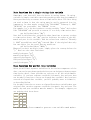
A data file is simply a computer file that has data in it. Most data files
are arranged like spreadsheets where you have lines of information from
each observation (a person, a state, or a company) and columns of
information representing different variables. The main difference
between a spreadsheet and a data file is that each column in a spreadsheet
is equal to one variable in a data file. Each variable of a data file is
made up of one or more columns. Sometimes the data file will have spaces
between the groups of columns that make up a variable, but most times it
will simply run everything together. Here is a sample spreadsheet:
Here is what the same information might look like in a data file:
12345678901234
123123.4 190
243 32.5
12
355 11.9383843
412 99
239
567123
4345
698 45.7
23
733 22.5
2
856 12
0
The first line of numbers isn't actually part of the data, we've put it
there so you can see how the columns in a data file relate to the columns
in a spreadsheet. In this example, column A in the spreadsheet is column
1 in the data file, column B is columns 2-3, column C is columns 4-8, and
column D is columns 9-14. If you look closely, you can see that the actual
numbers and letters are the same in both files. Since the information in
the data file are all run together you need some way of determining where
one variable ends and the next one starts. This, among many other important
things, is found in the codebook. This is the simplest format of a data
file and most will come like this. The two examples above have one "line,"
"record," or "card" of data for each observation. Often, though, a data
file will have more than one line of data for each observation. This is
a hold-over from the early days of computing when all the data were entered
on punch cards which had only 80 columns. If a survey had more questions
than could fit on one card, then researchers had to continue the data on
another card. This is particularly true for files that have information
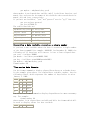
from the same observation for several years. Here is an example:
1 1991 12123
1 1992 45 34
1 1993 63 88
2 1991 34678
2 1992 55456
2 1993 76 44
3 1991 44234
3 1992 32 56
3 1993 67 55
This file is very much like the one above, except that each observation
has three lines in the file rather than just one. The information in a
specific column or columns may or may not represent the same variable.
If questions were dropped or added in subsequent years, then the
information will be different. Also, if it is an old data file, then it
is likely that each card is just a continuation of data from the same time
period.
A corollary to multiple cards is hierarchical files. Hierarchical files
typically have just one line of data for each observation, however, each
line may represent varying levels of information. Perhaps the best example
of a hierarchical file is the Current Population Survey. In the CPS file
there are three types of records or lines: Household records have
information that is common to everyone who lives in that household; Family
records have information that is common to everyone in a particular family
in that household (more than one family can live in a household); and
Person records have, of course, information pertaining to one specific
person in that family. All of this information is contained in one file.
The household record is always first, followed by the family record, and
finally the person record. Each line in the file has a variable or column
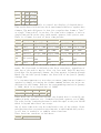
denoting what type of record it is. Here is an example of what a
hierarchical file might look like:
H 12 321
F 32 5 3
P 45 1 5
P 66 7 3
P 76 9 7
H 45 9 9
F678 3 5
F567 4 6
P8992187
P689 3 0
P66567 9
P554 5 9
P 89 8 9
Hierarchical files can be very tricky to program. If you need to analyze
a hierarchical file, you should come to the DSS lab and speak with a
consultant about how to do so. Of course, all of these examples have just
a few variables, whereas a real data file will have many, many more.
2.2 Codebooks
Now that we know what a data file is, we can make more sense out of what
a codebook is. A codebook is a technical description of the data that was
collected for a particular purpose. It describes how the data are arranged
in the computer file or files, what the various numbers and letters mean,
and any special instructions on how to use the data properly. Like any
other kind of "book," some codebooks are better than others. The best
codebooks have:
1. Description of the study: who did it, why they did it, how they did
it.
2. Sampling information: what was the population studied, how was the
sample drawn, what was the response rate.
3. Technical information about the files themselves: number of
observations, record length, number of records per observation,
etc.
4. Structure of the data within the file: hierarchical, multiple cards,
etc.
5. Details about the data: columns in which specific variables can be
found, whether they are character or numeric, and if numeric, what
format.
6. Text of the questions and responses: some even have how many people
responded a particular way.
Even though a codebook has (or at least, should have) all of this
information, not all codebooks will arrange it in the same manner. Later
in this document we will show you what information you will need to write
the program to read the data.
Before you decide on a particular dataset, there are some things you need
to verify before you can make good use of the data:
1. The wording and presence of the questions and answers. In a study
that is done repeatedly, the questions asked and the answers allowed
can change considerably from one "wave" to the next, not to mention
that some are dropped and new ones added. Also, subtle differences
in wording can mean very big changes in how you interpret your
results.
2. The sampling information. A survey that was conducted to measure
national attitudes toward a subject may not be good for assessing
those same attitudes in specific states.
3. Weights. Sometimes, in order to properly analyze the data, you will
need to apply weights to certain variables. These weights are
determined by the sampling procedure used to collect the data.
4. Flags. Flags perform a function similar to weights in the they tell
you if and when a special procedure was used to create the variable.
This is common when a person refuses or cannot answer a question,
but an interviewer can answer for them.
5. The column and line location of the variables in the file. This can
change from wave to wave also.
Once you have determined that a data file has what you want, you can begin
the task of writing the program that will extract or subset those variables
in which you are interested. The choice of which software package to use
is up to you. You should be aware, however, that most of Princeton's data
collection is accessible only on PUCC which has only SAS and SPSS. In any
case, it is always a good idea to talk to a Consultant before you try
extracting the data.
2.3 Writing the Program
Before you can write the program, you will need to be able to locate this
information about each variable you will want to use:
1. The column in which the variable you want starts.
2. The column in which it ends, or how many columns the variable
occupies.
3. Whether the variable is in numeric or character (also called
alphanumeric).
4. If the variable is numeric, how many decimal places it might have,
and if it is stored in a special format such as "zoned decimal."
5. If you are using data from several years, then you will need to make
sure that the above information is the same for each year. If it
is not, then you need to gather this information for each year.
Coding when there is just one line of data for each observation:
In many instances, the data file will have one record per observation.
In these instances, you will only need to know the column locations of
the variables you want. Here are two examples from the General Social
Survey Codebook:
This variable is coded as numeric and can be found in column 240 of the
data file. As you can see from the column labeled "PUNCH" above, there
are ten categories of responses to this question. Categories 8 ("Don't
know") and 9 ("No answer") are often re-coded by analysts to "missing"
so that they don't influence any of the statistics computed on this
variable. Depending on your specific questions, category 7 ("Other party,
refused to say") may also need to be coded as missing. Sometimes, variables
are entered as letters instead of numbers, such as if a person's name were
entered into the data file. In these instances, you must tell the computer
that there are letters instead of numbers. The example below shows how
to code this variable as if it were A) numeric and, B) character:
SAS:
SPSS:
Stata:
A) partyid 238 partyid 238
_column(238) partyid
_column(238) string
partyid
Although this codebook gives a name to the variable (partyid), not all
codebooks do. Sometimes the variables are simply numbered. You do not
always have to use the names or numbers provided as your own variable names,
however, using the ones provided will make referring to the codebook later
on much easier. This is important if you thought a variable should have
only two categories of responses, but five show up in the data; you may
have programmed the wrong columns or lines. It also allows comparison of
results of analyses conducted on the same data by different researchers.
Sometimes, the names provided are not allowable in whatever statistical
package you are using because they are too long or have special characters
B) partyid $ 238 partyid (a) 238
in them. In these cases, you should refer to the user manual of whatever
package you are using to determine what names are permissible. If you do
change the variable names, be sure to make a list of these changes.
Often, a variable must have more than one column, such as a person's age.
Here is an example of a variable that takes more than one column:
In this example, the variable can occupy two columns, 275-276 in the data
file. The coding for this is much the same as for the one above:
SAS:
SPSS:
Stata:
A)
polviewx
275-276
polviewx
275-276
_column(275-276)
polviewx
polviewx $
polviewx (a) _column(275-276) string
275-276
275-276
polviewx
If the variable were to have more than two columns, you would simply
specify the beginning and ending columns indicated. Sometimes, the
codebook will tell you in which column the variable begins and how many
columns it occupies (also referred to as its "length"). Look at this
example from the Current Population Survey :
D A-WKSLK 2 97 (00:99) Item 22C - 1) How many weeks has ... been looking
for work 2) How many weeks ago did ...start looking 3) How many weeks ago
was ...laid off
B)
It says that A-WKSLK is numeric, begins in column 97 and has a length of
2 (the instructions in the codebook explains this). In terms of the first
example, that means this variable can be found in columns 97-98. Character
variables would be indicated the same way. You can write the statements
to read these variables like the ones above (a_wkslk 97-98), but if you
have many variables, it would be time-consuming to calculate all the
specific columns. Instead, you could do it like this:
SAS:
SPSS:
Stata:
A) @97 a_wkslk 2.
a_wkslk 97
(f2.0)
_column(97) a_wkslk
%2f
_column(97) a_wkslk
%2s
You can readily see the similarities and differences among these. In all,
the "2" refers to the number of columns the variable occupies in the data
file, not necessarily how many digits there are in the variable (some
columns may be blank). This is especially important if your data has
decimals. For example, if a variable called "varname" were to have a length
of 5 and 2 decimal places in it, then the coding would be as follows:
SAS:
SPSS:
Stata:
B) @97 a_wkslk $2. a_wkslk 97 (a2)
@124 varname 5. varname 124
_column(124) varname
2
(f5.2)
%5.2f
This means that "varname" occupies a total of five columns in the data
file. Two of those columns are the numbers on the right of the decimal,
one is the decimal itself, and the last two columns are the numbers on
the left of the decimal. Therefore, the largest number that could be coded
into this space is 99.99. Once in a while, a codebook will tell you that
there are "implied" decimal places. This means that the decimal was not
actually entered into the data and you must assume (and correctly program)
that the last however many digits are on the right of the decimal.
Coding for more than one line of data for each observation:
You need to pay special attention to how many lines there are for each
observation, and on what line the variable you are interested in can be
found. Every codebook will indicate what line the variable can be found
differently, so you must look in the introductory pages to see how this
is done. Failure to keep track of what line the variable is on will result
in reading from the wrong line and thus, reading the wrong information
for that variable.
Let's assume that in Example 2 above, there are five lines of data for
each observation. Let's further assume that varname is found on the first
line for an observation and that charname is found on the third line. Here
are the statements you would need to read these variables:
SAS:
SPSS:
Stata:
data one;
data list
infile dictionary {
infile
file='mydata.dat'
_lines(5)
example n=5; records=5.
_line(1)
input
/1 varname 124-128
_column(124)
#1 @124
/3 charname 155-166 (a). varname %5f
varname 5.
_line(3)
_column(155) string
#3 @155
charname %12s
charname
}
$12.
As you can see, in each program you need to tell the program how many lines
there are for each observation ("n=5", "lines=5", and "_lines(5) ). Each
program also has a different way of identifying which line you want to
read ("#1", /1 , "_line(1)" ). If you wanted to read other variables from
lines 1 or 3, you could simply list them together without repeating the
line pointer for each variable. The program will continue reading from
the same line of data until you tell it to go to the next line.
2.4 Conclusion
This has been a brief and very general introduction to data files and
codebooks. We could not possibly cover everything you might encounter in
using a codebook. So, if you do find something you don't understand, ask
a consultant!
3. Interpreting Regression Output
3.1 Introduction
This guide assumes that you have at least a little familiarity with the
concepts of linear multiple regression, and are capable of performing a
regression in some software package such as Stata, SPSS or Excel. You may
wish to read our companion page Introduction to Regression first. For
assistance in performing regression in particular software packages,
there are some resources at UCLA Statistical Computing Portal.
Brief review of regression
Remember that regression analysis is used to produce an equation that will
predict a dependent variable using one or more independent variables. This
equation has the form
Y = b1X1 + b2X2 + ... + A
where Y is the dependent variable you are trying to predict, X1, X2 and
so on are the independent variables you are using to predict it, b1, b2
•
and so on are the coefficients or multipliers that describe the size of
the effect the independent variables are having on your dependent variable
Y, and A is the value Y is predicted to have when all the independent
variables are equal to zero.
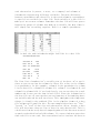
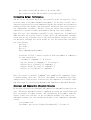
In the Stata regression shown below, the prediction equation is price =
-294.1955 (mpg) + 1767.292 (foreign) + 11905.42 - telling you that price
is predicted to increase 1767.292 when the foreign variable goes up by
one, decrease by 294.1955 when mpg goes up by one, and is predicted to
be 11905.42 when both mpg and foreign are zero.
Coming up with a prediction equation like this is only a useful exercise
if the independent variables in your dataset have some correlation with
your dependent variable. So in addition to the prediction components of
your equation--the coefficients on your independent variables (betas) and
the constant (alpha)--you need some measure to tell you how strongly each
independent variable is associated with your dependent variable.
When running your regression, you are trying to discover whether the
coefficients on your independent variables are really different from 0
(so the independent variables are having a genuine effect on your
dependent variable) or if alternatively any apparent differences from 0
are just due to random chance. The null (default) hypothesis is always
that each independent variable is having absolutely no effect (has a
coefficient of 0) and you are looking for a reason to reject this theory.
3.2 P, t and standard error
The t statistic is the coefficient divided by its standard error. The
standard error is an estimate of the standard deviation of the coefficient,
the amount it varies across cases. It can be thought of as a measure of
the precision with which the regression coefficient is measured. If a
coefficient is large compared to its standard error, then it is probably
different from 0.
How large is large? Your regression software compares the t statistic on
your variable with values in the Student's t distribution to determine
the P value, which is the number that you really need to be looking at.
The Student's t distribution describes how the mean of a sample with a
certain number of observations (your n) is expected to behave. For more
information on the t distribution, look at this web page.
If 95% of the t distribution is closer to the mean than the t-value on
the coefficient you are looking at, then you have a P value of 5%. This
is also reffered to a significance level of 5%. The P value is the
probability of seeing a result as extreme as the one you are getting (a
t value as large as yours) in a collection of random data in which the
variable had no effect. A P of 5% or less is the generally accepted point
at which to reject the null hypothesis. With a P value of 5% (or .05) there
is only a 5% chance that results you are seeing would have come up in a
random distribution, so you can say with a 95% probability of being correct
that the variable is having some effect, assuming your model is specified
correctly.
The 95% confidence interval for your coefficients shown by many regression
packages gives you the same information. You can be 95% confident that
the real, underlying value of the coefficient that you are estimating
falls somewhere in that 95% confidence interval, so if the interval does
not contain 0, your P value will be .05 or less.
Note that the size of the P value for a coefficient says nothing about
the size of the effect that variable is having on your dependent variable
- it is possible to have a highly significant result (very small P-value)
for a miniscule effect.
3.3 Coefficients
In simple or multiple linear regression, the size of the coefficient for
each independent variable gives you the size of the effect that variable
is having on your dependent variable, and the sign on the coefficient
(positive or negative) gives you the direction of the effect. In
regression with a single independent variable, the coefficient tells you
how much the dependent variable is expected to increase (if the
coefficient is positive) or decrease (if the coefficient is negative) when
that independent variable increases by one. In regression with multiple
independent variables, the coefficient tells you how much the dependent
variable is expected to increase when that independent variable increases
by one, holding all the other independent variables constant. Remember
to keep in mind the units which your variables are measured in.
Note: in forms of regression other than linear regression, such as
logistic or probit, the coefficients do not have this straightforward
interpretation. Explaining how to deal with these is beyond the scope of
an introductory guide.
3.4 R-Squared and overall significance of the
regression
The R-squared of the regression is the fraction of the variation in your
dependent variable that is accounted for (or predicted by) your
independent variables. (In regression with a single independent variable,
it is the same as the square of the correlation between your dependent
and independent variable.) The R-squared is generally of secondary
importance, unless your main concern is using the regression equation to
make accurate predictions. The P value tells you how confident you can
be that each individual variable has some correlation with the dependent
variable, which is the important thing.
Another number to be aware of is the P value for the regression as a whole.
Because your independent variables may be correlated, a condition known
as multicollinearity, the coefficients on individual variables may be
insignificant when the regression as a whole is significant. Intuitively,
this is because highly correlated independent variables are explaining
the same part of the variation in the dependent variable, so their
explanatory power and the significance of their coefficients is "divided
up" between them.
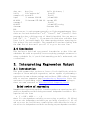
4.Introduction to Regression
4.1 Introduction
Regression analysis is used when you want to predict a continuous
dependent variable from a number of independent variables. If the
dependent variable is dichotomous, then logistic regression should be
used. (If the split between the two levels of the dependent variable is
close to 50-50, then both logistic and linear regression will end up giving
you similar results.) The independent variables used in regression can
be either continuous or dichotomous. Independent variables with more than
two levels can also be used in regression analyses, but they first must
be converted into variables that have only two levels. This is called dummy
coding and will be discussed later. Usually, regression analysis is used
with naturally-occurring variables, as opposed to experimentally
manipulated variables, although you can use regression with
experimentally manipulated variables. One point to keep in mind with
regression analysis is that causal relationships among the variables
cannot be determined. While the terminology is such that we say that X
"predicts" Y, we cannot say that X "causes" Y.
4.2 Assumptions of regression
Number of cases
When doing regression, the cases-to-Independent Variables (IVs) ratio
should ideally be 20:1; that is 20 cases for every IV in the model. The
lowest your ratio should be is 5:1 (i.e., 5 cases for every IV in the
model).
Accuracy of data
If you have entered the data (rather than using an established dataset),
it is a good idea to check the accuracy of the data entry. If you don't
want to re-check each data point, you should at least check the minimum
and maximum value for each variable to ensure that all values for each
variable are "valid." For example, a variable that is measured using a
1 to 5 scale should not have a value of 8.
Missing data
You also want to look for missing data. If specific variables have a lot
of missing values, you may decide not to include those variables in your
analyses. If only a few cases have any missing values, then you might want
to delete those cases. If there are missing values for several cases on
different variables, then you probably don't want to delete those cases
(because a lot of your data will be lost). If there are not too much missing
data, and there does not seem to be any pattern in terms of what is missing,
then you don't really need to worry. Just run your regression, and any
cases that do not have values for the variables used in that regression
will not be included. Although tempting, do not assume that there is no
pattern; check for this. To do this, separate the dataset into two groups:
those cases missing values for a certain variable, and those not missing
a value for that variable. Using t-tests, you can determine if the two
groups differ on other variables included in the sample. For example, you
might find that the cases that are missing values for the "salary" variable
are younger than those cases that have values for salary. You would want
to do t-tests for each variable with a lot of missing values. If there
is a systematic difference between the two groups (i.e., the group missing
values vs. the group not missing values), then you would need to keep this
in mind when interpreting your findings and not overgeneralize.
After examining your data, you may decide that you want to replace the
missing values with some other value. The easiest thing to use as the
replacement value is the mean of this variable. Some statistics programs
have an option within regression where you can replace the missing value
with the mean. Alternatively, you may want to substitute a group mean (e.g.,
the mean for females) rather than the overall mean.
The default option of statistics packages is to exclude cases that are
missing values for any variable that is included in regression. (But that
case could be included in another regression, as long as it was not missing
values on any of the variables included in that analysis.) You can change
this option so that your regression analysis does not exclude cases that
are missing data for any variable included in the regression, but then
you might have a different number of cases for each variable.
Outliers
You also need to check your data for outliers (i.e., an extreme value on
a particular item) An outlier is often operationally defined as a value
that is at least 3 standard deviations above or below the mean. If you
feel that the cases that produced the outliers are not part of the same
"population" as the other cases, then you might just want to delete those
cases. Alternatively, you might want to count those extreme values as
"missing," but retain the case for other variables. Alternatively, you
could retain the outlier, but reduce how extreme it is. Specifically, you
might want to recode the value so that it is the highest (or lowest)
non-outlier value.
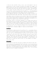
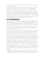
Normality
You also want to check that your data is normally distributed. To do this,
you can construct histograms and "look" at the data to see its distribution.
Often the histogram will include a line that depicts what the shape would
look like if the distribution were truly normal (and you can "eyeball"
how much the actual distribution deviates from this line). This histogram
shows that age is normally distributed:
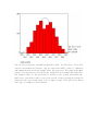
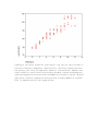
You can also construct a normal probability plot. In this plot, the actual
scores are ranked and sorted, and an expected normal value is computed
and compared with an actual normal value for each case. The expected normal
value is the position a case with that rank holds in a normal distribution.
The normal value is the position it holds in the actual distribution.
Basically, you would like to see your actual values lining up along the
diagonal that goes from lower left to upper right. This plot also shows
that age is normally distributed:
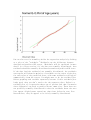
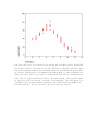
You can also test for normality within the regression analysis by looking
at a plot of the "residuals." Residuals are the difference between
obtained and predicted DV scores. (Residuals will be explained in more
detail in a later section.) If the data are normally distributed, then
residuals should be normally distributed around each predicted DV score.
If the data (and the residuals) are normally distributed, the residuals
scatterplot will show the majority of residuals at the center of the plot
for each value of the predicted score, with some residuals trailing off
symmetrically from the center. You might want to do the residual plot
before graphing each variable separately because if this residuals plot
looks good, then you don't need to do the separate plots. Below is a
residual plot of a regression where age of patient and time (in months
since diagnosis) are used to predict breast tumor size. These data are
not perfectly normally distributed in that the residuals about the zero
line appear slightly more spread out than those below the zero line.
Nevertheless, they do appear to be fairly normally distributed.
In addition to a graphic examination of the data, you can also
statistically examine the data's normality. Specifically, statistical
programs such as SPSS will calculate the skewness and kurtosis for each
variable; an extreme value for either one would tell you that the data
are not normally distributed. "Skewness" is a measure of how symmetrical
the data are; a skewed variable is one whose mean is not in the middle
of the distribution (i.e., the mean and median are quite different).
"Kurtosis" has to do with how peaked the distribution is, either too peaked
or too flat. "Extreme values" for skewness and kurtosis are values greater
than +3 or less than -3. If any variable is not normally distributed, then
you will probably want to transform it (which will be discussed in a later
section). Checking for outliers will also help with the normality problem.
Linearity
Regression analysis also has an assumption of linearity. Linearity means
that there is a straight line relationship between the IVs and the DV.
This assumption is important because regression analysis only tests for
a linear relationship between the IVs and the DV. Any nonlinear
relationship between the IV and DV is ignored. You can test for linearity
between an IV and the DV by looking at a bivariate scatterplot (i.e., a
graph with the IV on one axis and the DV on the other). If the two variables
are linearly related, the scatterplot will be oval.
Looking at the above bivariate scatterplot, you can see that friends is
linearly related to happiness. Specifically, the more friends you have,
the greater your level of happiness. However, you could also imagine that
there could be a curvilinear relationship between friends and happiness,
such that happiness increases with the number of friends to a point. Beyond
that point, however, happiness declines with a larger number of friends.
This is demonstrated by the graph below:
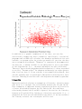
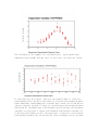
You can also test for linearity by using the residual plots described
previously. This is because if the IVs and DV are linearly related, then
the relationship between the residuals and the predicted DV scores will
be linear. Nonlinearity is demonstrated when most of the residuals are
above the zero line on the plot at some predicted values, and below the
zero line at other predicted values. In other words, the overall shape
of the plot will be curved, instead of rectangular. The following is a
residuals plot produced when happiness was predicted from number of
friends and age. As you can see, the data are not linear:
The following is an example of a residuals plot, again predicting
happiness from friends and age. But, in this case, the data are linear:
If your data are not linear, then you can usually make it linear by
transforming IVs or the DV so that there is a linear relationship between
them. Sometimes transforming one variable won't work; the IV and DV are
just not linearly related. If there is a curvilinear relationship between
the DV and IV, you might want to dichotomize the IV because a dichotomous
variable can only have a linear relationship with another variable (if
it has any relationship at all). Alternatively, if there is a curvilinear
relationship between the IV and the DV, then you might need to include
the square of the IV in the regression (this is also known as a quadratic
regression).
The failure of linearity in regression will not invalidate your analysis
so much as weaken it; the linear regression coefficient cannot fully
capture the extent of a curvilinear relationship. If there is both a
curvilinear and a linear relationship between the IV and DV, then the
regression will at least capture the linear relationship.
Homoscedasticity
The assumption of homoscedasticity is that the residuals are
approximately equal for all predicted DV scores. Another way of thinking
of this is that the variability in scores for your IVs is the same at all
values of the DV. You can check homoscedasticity by looking at the same
residuals plot talked about in the linearity and normality sections. Data
are homoscedastic if the residuals plot is the same width for all values
of the predicted DV. Heteroscedasticity is usually shown by a cluster of
points that is wider as the values for the predicted DV get larger.
Alternatively, you can check for homoscedasticity by looking at a
scatterplot between each IV and the DV. As with the residuals plot, you
want the cluster of points to be approximately the same width all over.
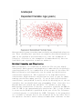
The following residuals plot shows data that are fairly homoscedastic.
In fact, this residuals plot shows data that meet the assumptions of
homoscedasticity, linearity, and normality (because the residual plot is
rectangular, with a concentration of points along the center):
Heteroscedasiticy may occur when some variables are skewed and others are
not. Thus, checking that your data are normally distributed should cut
down on the problem of heteroscedasticity. Like the assumption of
linearity, violation of the assumption of homoscedasticity does not
invalidate your regression so much as weaken it.
Multicollinearity and Singularity
Multicollinearity is a condition in which the IVs are very highly
correlated (.90 or greater) and singularity is when the IVs are perfectly
correlated and one IV is a combination of one or more of the other IVs.
Multicollinearity and singularity can be caused by high bivariate
correlations (usually of .90 or greater) or by high multivariate
correlations. High bivariate correlations are easy to spot by simply
running correlations among your IVs. If you do have high bivariate
correlations, your problem is easily solved by deleting one of the two
variables, but you should check your programming first, often this is a
mistake when you created the variables. It's harder to spot high
multivariate correlations. To do this, you need to calculate the SMC for
each IV. SMC is the squared multiple correlation ( R2 ) of the IV when
it serves as the DV which is predicted by the rest of the IVs. Tolerance,
a related concept, is calculated by 1-SMC. Tolerance is the proportion
of a variable's variance that is not accounted for by the other IVs in
the equation. You don't need to worry too much about tolerance in that
most programs will not allow a variable to enter the regression model if
tolerance is too low.
Statistically, you do not want singularity or multicollinearity because
calculation of the regression coefficients is done through matrix
inversion. Consequently, if singularity exists, the inversion is
impossible, and if multicollinearity exists the inversion is unstable.
Logically, you don't want multicollinearity or singularity because if
they exist, then your IVs are redundant with one another. In such a case,
one IV doesn't add any predictive value over another IV, but you do lose
a degree of freedom. As such, having multicollinearity/ singularity can
weaken your analysis. In general, you probably wouldn't want to include
two IVs that correlate with one another at .70 or greater.
4.3 Transformations
As mentioned in the section above, when one or more variables are not
normally distributed, you might want to transform them. You could also
use transformations to correct for heteroscedasiticy, nonlinearity, and
outliers. Some people do not like to do transformations because it becomes
harder to interpret the analysis. Thus, if your variables are measured
in "meaningful" units, such as days, you might not want to use
transformations. If, however, your data are just arbitrary values on a
scale, then transformations don't really make it more difficult to
interpret the results.
Since the goal of transformations is to normalize your data, you want to
re- check for normality after you have performed your transformations.
Deciding which transformation is best is often an exercise in
trial-and-error where you use several transformations and see which one
has the best results. "Best results" means the transformation whose
distribution is most normal. The specific transformation used depends on
the extent of the deviation from normality. If the distribution differs
moderately from normality, a square root transformation is often the best.
A log transformation is usually best if the data are more substantially
non-normal. An inverse transformation should be tried for severely
non-normal data. If nothing can be done to "normalize" the variable, then
you might want to dichotomize the variable (as was explained in the
linearity section). Direction of the deviation is also important. If the
data is negatively skewed, you should "reflect" the data and then apply
the transformation. To reflect a variable, create a new variable where
the original value of the variable is subtracted from a constant. The
constant is calculated by adding 1 to the largest value of the original
variable.
If you have transformed your data, you need to keep that in mind when
interpreting your findings. For example, imagine that your original
variable was measured in days, but to make the data more normally
distributed, you needed to do an inverse transformation. Now you need to
keep in mind that the higher the value for this transformed variable, the
lower the value the original variable, days. A similar thing will come
up when you "reflect" a variable. A greater value for the original variable
will translate into a smaller value for the reflected variable.
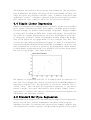
4.4 Simple Linear Regression
Simple linear regression is when you want to predict values of one variable,
given values of another variable. For example, you might want to predict
a person's height (in inches) from his weight (in pounds). Imagine a sample
of ten people for whom you know their height and weight. You could plot
the values on a graph, with weight on the x axis and height on the y axis.
If there were a perfect linear relationship between height and weight,
then all 10 points on the graph would fit on a straight line. But, this
is never the case (unless your data are rigged). If there is a (nonperfect)
linear relationship between height and weight (presumably a positive one),
then you would get a cluster of points on the graph which slopes upward.
In other words, people who weigh a lot should be taller than those people
who are of less weight. (See graph below.)
The purpose of regression analysis is to come up with an equation of a
line that fits through that cluster of points with the minimal amount of
deviations from the line. The deviation of the points from the line is
called "error." Once you have this regression equation, if you knew a
person's weight, you could then predict their height. Simple linear
regression is actually the same as a bivariate correlation between the
independent and dependent variable.
4.5 Standard Multiple Regression
Standard multiple regression is the same idea as simple linear regression,
except now you have several independent variables predicting the
dependent variable. To continue with the previous example, imagine that
you now wanted to predict a person's height from the gender of the person
and from the weight. You would use standard multiple regression in which
gender and weight were the independent variables and height was the
dependent variable. The resulting output would tell you a number of things.
First, it would tell you how much of the variance of height was accounted
for by the joint predictive power of knowing a person's weight and gender.
This value is denoted by "R2". The output would also tell you if the model
allows you to predict a person's height at a rate better than chance. This
is denoted by the significance level of the overall F of the model. If
the significance is .05 (or less), then the model is considered
significant. In other words, there is only a 5 in a 100 chance (or less)
that there really is not a relationship between height and weight and
gender. For whatever reason, within the social sciences, a significance
level of .05 is often considered the standard for what is acceptable. If
the significance level is between .05 and .10, then the model is considered
marginal. In other words, the model is fairly good at predicting a person's
height, but there is between a 5-10% probability that there really is not
a relationship between height and weight and gender.
In addition to telling you the predictive value of the overall model,
standard multiple regression tells you how well each independent variable
predicts the dependent variable, controlling for each of the other
independent variables. In our example, then, the regression would tell
you how well weight predicted a person's height, controlling for gender,
as well as how well gender predicted a person's height, controlling for
weight.
To see if weight was a "significant" predictor of height you would look
at the significance level associated with weight on the printout. Again,
significance levels of .05 or lower would be considered significant, and
significance levels .05 and .10 would be considered marginal. Once you
have determined that weight was a significant predictor of height, then
you would want to more closely examine the relationship between the two
variables. In other words, is the relationship positive or negative? In
this example, we would expect that there would be a positive relationship.
In other words, we would expect that the greater a person's weight, the
greater his height. (A negative relationship would be denoted by the case
in which the greater a person's weight, the shorter his height.) We can
determine the direction of the relationship between weight and height by
looking at the regression coefficient associated with weight. There are
two kinds of regression coefficients: B (unstandardized) and beta
(standardized). The B weight associated with each variable is given in
terms of the units of this variable. For weight, the unit would be pounds,
and for height, the unit is inches. The beta uses a standard unit that
is the same for all variables in the equation. In our example, this would
be a unit of measurement that would be common to weight and height. Beta
weights are useful because then you can compare two variables that are
measured in different units, as are height and weight.
If the regression coefficient is positive, then there is a positive
relationship between height and weight. If this value is negative, then
there is a negative relationship between height and weight. We can more
specifically determine the relationship between height and weight by
looking at the beta coefficient for weight. If the beta = .35, for example,
then that would mean that for one unit increase in weight, height would
increase by .35 units. If the beta=-.25, then for one unit increase in
weight, height would decrease by .25 units. Of course, this relationship
is valid only when holding gender constant.
A similar procedure would be done to see how well gender predicted height.
However, because gender is a dichotomous variable, the interpretation of
the printouts is slightly different. As with weight, you would check to
see if gender was a significant predictor of height, controlling for
weight. The difference comes when determining the exact nature of the
relationship between gender and height. That is, it does not make sense
to talk about the effect on height as gender increases or decreases, since
gender is not a continuous variable (we would hope). Imagine that gender
had been coded as either 0 or 1, with 0 = female and 1=male. If the beta
coefficient of gender were positive, this would mean that males are taller
than females. If the beta coefficient of gender were negative, this would
mean that males are shorter than females. Looking at the magnitude of the
beta, you can more closely determine the relationship between height and
gender. Imagine that the beta of gender were .25. That means that males
would be .25 units taller than females. Conversely, if the beta
coefficient were -.25, this would mean that males were .25 units shorter
than females. Of course, this relationship would be true only when
controlling for weight.
As mentioned, the significance levels given for each independent variable
indicates whether that particular independent variable is a significant
predictor of the dependent variable, over and above the other independent
variables. Because of this, an independent variable that is a significant
predictor of a dependent variable in simple linear regression may not be
significant in multiple regression (i.e., when other independent
variables are added into the equation). This could happen because the
variance that the first independent variable shares with the dependent
variable could overlap with the variance that is shared between the second
independent variable and the dependent variable. Consequently, the first
independent variable is no longer uniquely predictive and thus would not
show up as being significant in the multiple regression. Because of this,
it is possible to get a highly significant R2, but have none of the
independent variables be significant.
5. Working With Dummy Variables
5.1 Why use dummies?
Regression analysis is used with numerical variables. Results only have
a valid interpretation if it makes sense to assume that having a value
of 2 on some variable is does indeed mean having twice as much of something
as a 1, and having a 50 means 50 times as much as 1.
However, social scientists often need to work with categorical variables
in which the different values have no real numerical relationship with
each other. Examples include variables for race, political affiliation,
or marital status. If you have a variable for political affiliation with
possible responses including Democrat, Independent, and Republican, it
obviously doesn't make sense to assign values of 1 - 3 and interpret that
as meaning that a Republican is somehow three times as politically
affiliated as a Democrat.
The solution is to use dummy variables - variables with only two values,
zero and one. It does make sense to create a variable called "Republican"
and interpret it as meaning that someone assigned a 1 on this varible is
Republican and someone with an 0 is not.
5.2 Nominal variables with multiple levels
If you have a nominal variable that has more than two levels, you need
to create multiple dummy variables to "take the place of" the original
nominal variable. For example, imagine that you wanted to predict
depression from year in school: freshman, sophomore, junior, or senior.
Obviously, "year in school" has more than two levels.
What you need to do is to recode "year in school" into a set of dummy
variables, each of which has two levels. The first step in this process
is to decide the number of dummy variables. This is easy; it's simply k-1,
where k is the number of levels of the original variable.
You could also create dummy variables for all levels in the original
variable, and simply drop one from each analysis.
In this instance, we would need to create 4-1=3 dummy variables. In order
to create these variables, we are going to take 3 of the levels of "year
of school", and create a variable corresponding to each level, which will
have the value of yes or no (i.e., 1 or 0). In this instance, we can create
a variable called "sophomore," "junior," and "senior." Each instance of
"year of school" would then be recoded into a value for "sophomore,"
"junior," and "senior." If a person were a junior, then "sophomore" would
be equal to 0, "junior" would be equal to 1, and "senior" would be equal
to 0.
5.3 Interpreting results
The decision as to which level is not coded is often arbitrary. The level
which is not coded is the category to which all other categories will be
compared. As such, often the biggest group will be the not- coded category.
For example, often "Caucasian" will be the not-coded group if that is the
race of the majority of participants in the sample. In that case, if you
have a variable called "Asian", the coefficient on the "Asian" variable
in your regression will show the effect being Asian rather than Caucasian
has on your dependant variable.
In our example, "freshman" was not coded so that we could determine if
being a sophomore, junior, or senior predicts a different depressive level
than being a freshman. Consequently, if the variable, "junior" was
significant in our regression, with a positive beta coefficient, this
would mean that juniors are significantly more depressed than freshman.
Alternatively, we could have decided to not code "senior," if we thought
that being a senior is qualitatively different from being of another year.
For further information, see Regression with Stata chapter 3, Regression
with Categorical Variables
6.Time Series Data in Stata
6.1 Time series data and tsset
To use Stata's time-series functions and analyses, you must first make
sure that your data are, indeed, time-series. First, you must have a date
variable that is in Stata date format. Secondly, you must make sure that
your data are sorted by this date variable. If you have panel data, then
your data must be sorted by the date variable within the variable that
identifies the panel. Finally, you must use the tsset command to tell Stata
that your data are time-series:
sort datevar
tsset datevar
or
sort panelvar datevar
tsset panelvar datevar
The first example tells Stata that you have simple time-series data, and
the second tells Stata that you have panel data.
6.2 Stata Date Format
Stata stores dates as the number of elapsed days since January 1, 1960.
There are different ways to create elapsed Stata dates that depend on how
dates are represented in your data. If your original dataset already
contains a single date variable, then use the date() function or one of
the other string-date commands. If you have separate variables storing
different parts of the date (month, day and year; year and quarter, etc.)
then you will need to use the partial date variable functions.
Date functions for a single string date variable
Sometimes, your data will have the dates in string format. (A string
variable is simply a variable containing anything other than just numbers.)
Stata provides a way to convert these to time-series dates. The first thing
you need to know is that the string must be easily separated into its
components. In other words, strings like "01feb1990" "February 1, 1990"
"02/01/90" are acceptable, but "020190" is not.
For example, let's say that you have a string variable "sdate" with values
like "01feb1990" and you need to convert it to a daily time-series date:
gen daily=date(sdate,"dmy")
Note that in this function, as with the other functions to convert strings
to time-series dates, the "dmy" portion indicates the order of the day,
month and year in the variable. Had the values been coded as "February
1, 1990" we would have used "mdy" instead. What if the original date only
has two digits for the year? Then we would use:
gen daily=date(sdate,"dm19y")
Whenever you have two digit years, simply place the century before the
"y." Here are the other functions:
weekly(stringvar,"wy")
monthly(stringvar,"my")
quarterly(stringvar,"qy")
halfyearly(stringvar,"hy")
yearly(stringvar,"y")
Date functions for partial date variables
Often you will have separate variables for the various components of the
date; you need to put them together before you can designate them as proper
time-series dates. Stata provides an easy way to do this with numeric
variables. If you have separate variables for month, day and year then
use the mdy() function to create an elapsed date variable. Once you have
created an elapsed date variable, you will probably want to format it,
as described below.
Use the mdy() function to create an elapsed Stata date variable when your
original data contains separate variables for month, day and year. The
month, day and year variables must be numeric. For example, suppose you
are working with these data:
month day year
7
11 1948
1
21 1952
11
2
8
12 1993
1994
Use the following Stata command to generate a new variable named mydate:
gen mydate = mdy(month,day,year)
where mydate is an elapsed date varible, mdy() is the Stata function, and
month, day, and year are the names of the variables that contain data for
month, day and year, respectively.
If you have two variables, "year" and "quarter" use the "yq()" function:
gen qtr=yq(year,quarter)
gen qtr=yq(1990,3)
The other functions are:
mdy(month,day,year) for daily data
yw(year, week)
for weekly data
ym(year,month)
for monthly data
yq(year,quarter)
for quarterly data
yh(year,half-year) for half-yearly data
Converting a date variable stored as a single number
If you have a date variable where the date is stored as a single number
of the form yyyymmdd (for example, 20041231 for December 31, 2004) the
following set of functions will convert it into a Stata elapsed date.
gen year = int(date/10000)
gen month = int((date-year*10000)/100)
gen day = int((date-year*10000-month*100))
gen mydate = mdy(month,day,year)
format mydate %d
Time series date formats
Use the format command to display elapsed Stata dates as calendar dates.
In the example given above, the elapsed date variable, mydate, has the
following values, which represent the number of days before or after
January 1, 1960.
month day year mydate
7
11 1948 -4191
1
21 1952 -2902
8
12 1993 12277
11
2
1994 12724
You can use the format command to display elapsed dates in a more customary
way. For example:
format mydate %d
where mydate is an elapsed date variable and %d is the format which will
be used to display values for that variable.
month day year mydate
7
11 1948 11jul48
1
21 1952 21jan52
8
12 1993 12aug93
11
2
1994 02nov94
Other formats are available to control the display of elapsed dates.
Time-series dates in Stata have their own formats similar to regular date
formats. The main difference is that for a regular date format a "unit"
or single "time period" is one day. For time series formats, a unit or
single time period can be a day, week, month, quarter, half-year or year.
There is a format for each of these time periods:
Format Description Beginning
+1 Unit
+2 Units
+3 Units
%td
daily
01jan1960
02jan1960
03Jan1960
04Jan1960
%tw
weekly
week 1, 1960 week 2, 1960 week 3, 1960 week 4, 1960
%tm
monthly
Jan, 1960
%tq
quarterly
1st qtr, 1960 2nd qtr, 1960 3rd qtr, 1960 4th qtr, 1961
%th
half-yearly
1st half,
1960
2nd half,
1960
1st half,
1961
2nd half,
1961
%ty
yearly
1960
1961
1962
1963
Feb, 1960
Mar, 1960
Apr, 1960
You should note that in the weekly format, the year is divided into 52
weeks. The first week is defined as the first seven days, regardless of
what day of the week it may be. Also, the last week, week 52, may have
8 or 9 days. For the quarterly format, the first quarter is January through
March. For the half-yearly format, the first half of the year is January
through June.
It's even more important to note that you cannot jump from one format to
another by simply re-issuing the format command because the units are
different in each format. Here are the corresponding results for January
1, 1999, which is an elapsed date of 14245:
%td
%tw
%tq
%th
%ty
01jan1999 2233w50 5521q2 9082h2
These dates are so different because the elapsed date is actually the
number of weeks, quarters, etc., from the first week, quarter, etc of 1960.
The value for %ty is missing because it would be equal to the year 14,245
which is beyond what Stata can accept.
Any of these time units can be translated to any of the others. Stata
provides functions to translate any time unit to and from %td daily units,
so all that is needed is to combine these functions.
These functions translate to %td dates:
dofw() weekly to daily
dofm() monthly to daily
dofq() quarterly to daily
dofy() yearly to daily
These functions translate from %td dates:
wofd() daily to weekly
mofd() daily to monthly
qofd() daily to quarterly
yofd() daily to yearly
For more information see the Stata User's Guide, chapter 27.
Specifying dates
Often we need to consuct a particular analysis only on observations that
fall on a certain date. To do this, we have to use something called a date
literal. A date literal is simply a way of entering a date in words and
have Stata automatically convert it to an elapsed date. As with the d()
literal to specify a regular date, there are the w(), m(), q(), h(), and
y() literals for entering weekly, monthly, quarterly, half-yearly, and
yearly dates, respectively. Here are some examples:
reg x y if w(1995w9)
sum income if q(1988-3)
tab gender if y(1999)
If you want to specify a range of dates, you can use the tin() and twithin()
functions:
reg y x if tin(01feb1990,01jun1990)
sum income if twithin(1988-3,1998-3)
The difference between tin() and twithin() is that tin() includes the
beginning and end dates, whereas twithin() excludes them. Always enter
the beginning date first, and write them out as you would for any of the
d(), w(), etc. functions.
6.3 Time Series Variable Lists
Often in time-series analyses we need to "lag" or "lead" the values of
a variable from one observation to the next. If we have many variables,
this can be cumbersome, especially if we need to lag a variable more than
once. In Stata, we can specify which variables are to be lagged and how
many times without having to create new variables, thus saving alot of
disk space and memory. You should note that the tsset command must have
been issued before any of the "tricks" in this section will work. Also,
if you have defined your data as panel data, Stata will automatically
re-start the calculations as it comes to the beginning of a panel so you
need not worry about values from one panel being carried over to the next.
L.varname and F.varname
If you need to lag or lead a variable for an analysis, you can do so by
using the L.varname (to lag) and F.varname (to lead). Both work the same
way, so we'll just show some examples with L.varname. Let's say you want
to regress this year's income on last year's income:
reg income L.income
would accomplish this. The "L." tells Stata to lag income by one time
period. If you wanted to lag income by more than one time period, you would
simply change the L. to something like "L2." or "L3." to lag it by 2 and
3 time periods, respectively. The following two commands will produce the
same results:
reg income L.income L2.income L3.income
reg income L(1/3).income
D.varname
Another useful shortcut is D.varname, which takes the difference of income
in time 1 and income in time 2. For example, let's say a person earned
$20 yesterday and $30 today.
Date
income D.income D2.income
02feb1999 20
.
.
02mar1999 30
10
.
02apr1999 45
15
5
So, you can see that D.=(income-incomet-1) and
D2=(income-incomet-1)-(incomet-1-incomet-2)
S.varname
S.varname refers to seasonal differences and works like D.varname, except
that the difference is always taken from the current observation to the
nth observation:
Date
income S.income S2.income
02feb1999 20
.
.
02mar1999 30
10
.
02apr1999 45
15
25
In other words: S.income=income-incomet-1 and S2.income=income-incomet-2
7. Lag Selection in Time Series Data
When running regressions on time-series data, it is often important to
include lagged values of the dependent variable as independant variables.
In technical terminology, the regression is now called a vector
autoregression (VAR). For example, when trying to sort out the dterminants
of GDP, it is likely that last year's GDP is correlated with this year's
GDP. If this is the case, GDP lagged for at least one year should be
included on the right-hand side of the regression.
If the variable in question is persistent--that is, values in the far past
are still affecting today's values--more lags will be necessary. In order
to determine how many lags to use, several selection criteria can be used.
The two most common are the Akaike Information Criterion (AIC) and the
Schwarz' Bayesian Information Criterion (SIC/BIC/SBIC). These rules
choose lag length j to minimize: log(SSR(j)/n) + (j + 1)C(n)/n, where SSR(j)
is the sum or squared residuals for the VAR with j lags and n is the number
of observations; C(n) = 2 for AIC and C(n) = log(n) for BIC.
Fortunately, in Stata 8 there is a single command that will do the math
for any number of specified lags: varsoc. To get the AIC and BIC, simply
type 'varsoc depvar' in the command window. The default number of lags
Stata checks is 4; in order to check a different number, add ',
maxlags(#oflags)' after the 'varsoc depvar'. If, in addition, the
regression has independent variables other than the lags, include those
after the 'maxlag()' option by typing 'exog(varnames)'. The output will
indicate the optimal lag number with an asterisk. Then proceed to run the
regression using the specified number of lags on the dependent variable
on the right-hand side with the other independent variables.
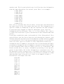
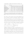
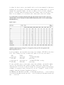
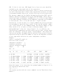
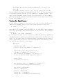
Example:
varsoc y, maxlag(5) exog(x z)
Selection order criteria
endogenous variables:
y
exogenous variables:
x z
constant included in models
Sample:
6
20
Obs = 15
--------------------------------------------------------------------lag
LL
LR
df
p
FPE
AIC
HQIC
SBIC
--------------------------------------------------------------------0 -45.854
.
.
.
39.70191
6.51381 6.5123
6.65542
1 -35.849 20.009* 1 0.000 12.04354* 5.31319* 5.31118* 5.50201*
2 -35.837 0.024
1 0.877 13.92282
5.44493 5.44241 5.68094
3 -35.305 1.063
1 0.302 15.13169
5.50737 5.50435 5.79059
4 -35.233 0.145
1 0.703 17.66201
5.63103 5.62751 5.96145
5 -35.108 0.250
1 0.617 20.7534
5.74767 5.74365 6.1253
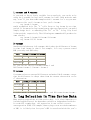
--------------------------------------------------------------------From this output, it is clear that the optimal number of lags is 1, so
the regression should look like:
reg y l.y x z
(For further options with the varsoc command, see the Time-Series Stata
manual.)
8. Panel Data
8.1 Introduction
Panel data, also called longitudinal data or cross-sectional time series
data, are data where multiple cases (people, firms, countries etc) were
observed at two or more time periods. An example is the National
Longitudinal Survey of Youth, where a nationally representative sample
of young people were each surveyed repeatedly over multiple years.
There are two kinds of information in cross-sectional time-series data:
the cross-sectional information reflected in the differences between
subjects, and the time-series or within-subject information reflected in
the changes within subjects over time. Panel data regression techniques
allow you to take advantage of these different types of information.
While it is possible to use ordinary multiple regression techniques on
panel data, they may not be optimal. The estimates of coefficients derived
from regression may be subject to omitted variable bias - a problem that
arises when there is some unknown variable or variables that cannot be
controlled for that affect the dependent variable. With panel data, it
is possible to control for some types of omitted variables even without
observing them, by observing changes in the dependent variable over time.
This controls for omitted variables that differ between cases but are
constant over time. It is also possible to use panel data to control for
omitted variables that vary over time but are constant between cases.
8.2 Using Panel Data in Stata
A panel dataset should have data on n cases, over t time periods, for a
total of n × t observations. Data like this is said to be in long form.
In some cases your data may come in what is called the wide form, with
only one observation per case and variables for each different value at
each different time period. To analyze data like this in Stata using
commands for panel data analysis, you need to first convert it to long
form. This can be done using Stata's reshape command. For assistance in
using reshape, see Stata's online help or this web page.
Stata provides a number of tools for analyzing panel data. The commands
all begin with the prefix xt and include xtreg, xtprobit, xtsum and xttab
- panel data versions of the familiar reg, probit, sum and tab commands.
To use these commands, first tell Stata that your dataset is panel data.
You need to have a variable that identifies the case element of your panel
(for example, a country or person identifier) and also a time variable
that is in Stata date format. For information about Stata's date variable
formats, see our Time Series Data in Stata page.
Sort your data by the panel variable and then by the date variable within
the panel variable. Then you need to issue the tsset command to identify
the panel and date variables. If your panel variable is called panelvar
and your date variable is called datevar, the commands needed are:
. sort panelvar datevar
. tsset panelvar datevar
If you prefer to use menus, use the command under Statistics > Time Series
> Setup and Utilities > Declare Data to be Time Series.
8.3 Fixed, Between and Random Effects models
Fixed Effects Regression
Fixed effects regression is the model to use when you want to control for
omitted variables that differ between cases but are constant over time.
It lets you use the changes in the variables over time to estimate the
effects of the independent variables on your dependent variable, and is
the main technique used for analysis of panel data.
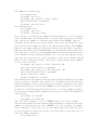
The command for a linear regression on panel data with fixed effects in
Stata is xtreg with the fe option, used like this:
xtreg dependentvar independentvar1 independentvar2
independentvar3 ... , fe
If you prefer to use the menus, the command is under Statistics >
Cross-sectional time series > Linear models > Linear regression.
This is equivalent to generating dummy variables for each of your cases
and including them in a standard linear regression to control for these
fixed "case effects". It works best when you have relatively fewer cases
and more time periods, as each dummy variable removes one degree of freedom
from your model.
Between Effects
Regression with between effects is the model to use when you want to
control for omitted variables that change over time but are constant
between cases. It allows you to use the variation between cases to estimate
the effect of the omitted independent variables on your dependent
variable.
The command for a linear regression on panel data with between effects
in Stata is xtreg with the be option.
Running xtreg with between effects is equivalent to taking the mean of
each variable for each case across time and running a regression on the
collapsed dataset of means. As this results in loss of information,
between effects are not used much in practice. Researchers who want to
look at time effects without considering panel effects generally will use
a set of time dummy variables, which is the same as running time fixed
effects.
The between effects estimator is mostly important because it is used to
produce the random effects estimator.
Random Effects
If you have reason to believe that some omitted variables may be constant
over time but vary between cases, and others may be fixed between cases
but vary over time, then you can include both types by using random effects.
Stata's random-effects estimator is a weighted average of fixed and
between effects.
The command for a linear regression on panel data with random effects in
Stata is xtreg with the re option.
8.4 Choosing Between Fixed and Random Effects
The generally accepted way of choosing between fixed and random effects
is running a Hausman test.
Statistically, fixed effects are always a reasonable thing to do with
panel data (they always give consistent results) but they may not be the
most efficient model to run. Random effects will give you better P-values
as they are a more efficient estimator, so you should run random effects
if it is statistcally justifiable to do so.
The Hausman test checks a more efficient model against a less efficient
but consistent model to make sure that the more efficient model also gives
consistent results.
To run a Hausman test comparing fixed with random effects in Stata, you
need to first estimate the fixed effects model, save the coefficients so
that you can compare them with the results of the next model, estimate
the random effects model, and then do the comparison.
. xtreg dependentvar independentvar1 independentvar2
independentvar3 ... , fe
. estimates store fixed
. xtreg dependentvar independentvar1 independentvar2
independentvar3 ... , re
. estimates store random
. hausman fixed random
The hausman test tests the null hypothesis that the coefficients estimated
by the efficient random effects estimator are the same as the ones
estimated by the consistent fixed effects estimator. If they are
(insignificant P-value, Prob>chi2 larger than .05) then it is safe to use
random effects. If you get a significant P-value, however, you should use
fixed effects
9. Event Studies with Stata
An event study is used to examine reactions over time to events of
interest. A simple event study involves the following steps:
• Identifying the event of interest and defining an event window
• Selecting a set of cases to include in the analysis
Predicting a "normal" outcome during the event window in the absence
of the event
• Estimating the cumulative abnormal outcome within the event window,
where the cumulative abnormal return is defined as the difference
between the actual and predicted returns during the event window
• Testing whether the cumulative abnormal return is statistically
different from zero.
This document is designed to help you conduct event studies in Stata. It
uses CRSP stock exchange data as examples, although it can be easily
extended to other types of data in other fields. We assume that you already
have the data you need and that you have a basic familiarity with Stata.
If you need assistance with Stata commands, you can find out more about
it here.
Your task will be much easier if you enter the commands in a do file, which
is a text file containing a list of Stata commands.
•
Adding the Event Date
If your data does not already have the event date included, you will need
to add it before you can continue. This is a very simple process:
1. Enter the event dates along with the company ID in a spreadsheet
such as Excel. Be sure to label the column with the dates something
other than "date," such as "evdate." You need only one line for each
company. Convert the file to Stata.
2. Put the date in Stata date format. Instructions on converting date
variables to Stata format can be found here.
Note: This is an important step. If you don't do this, you will not
be able to sort on date and your results will be wrong.
3. In Stata, sort this file according to PERMNO and EVDATE:
sort permno evdate
4. Save this file and call it something like "evdates."
5. "Use" your main data file and sort it by PERMNO and DATE.
6. Merge the two datasets:
merge permno using evdates
7. Save the file.
Cleaning the data and Calculating the Event and Estimation
Windows
It's likely that you have more observations for each company than you need.
It's also possible that you do not have enough for some. Before you can
continue, you must make sure that you will be conducting your analyses
on the correct observations. To do this, you will need to create a variable
that will count the number of days from the observation to the event date.
This can be either calendar days or weekdays.
For number of trading days:
sort permno date
by permno: gen id=_n
by permno: gen targ=id if date==evdate
egen td=min(targ), by(permno)
by permno: gen dif=id-td
For calendar days:
sort permno date
by permno: gen id=_n
by permno: dif=date-evdate
As you can see, calculating the number of trading days is a little trickier
than calendar days. For trading days, we first need to create a variable
that counts the number of observations within each PERMNO. Then we
determine which observation occurs on the event date. We assign the event
date's observation number to all of the observations within that PERMNO.
Finally, we simply take the difference between the two. Next, we need to
make sure that we have the minimum number of observations before and after
the event date, as well as the minimum number of observations before the
event window for the estimation window. Let's say we want 30 days before
and after the event date (a total of 61 days in the event window) and 30
days for the estimation window. (You can of course change these numbers
to suit your analysis.)
by permno: gen evwin=1 if dif>=-30 & dif<=30
egen evobs=count(evwin), by(permno)
by permno: gen estwin=1 if dif<-30 & dif>=-60
egen estobs=count(estwin), by(permno)
replace evwin=0 if evwin==.
replace estwin=0 if estwin==.
The procedure for determining the event and estimation windows is the same.
First we create a variable that equals 1 if the observation is within the
specified number of days. Second, we create another variable that counts
how many observations, within each PERMNO, has a 1 assigned to it. Finally,
we replace all the missing values with zeroes, creating a dummy variable.
You can now determine which companies do not have a sufficient number of
observations.
tab permno if evobs<61
tab permno if estobs<30
The "tab" will produce a list of PERMNOs that do not have enough
observations within the event and estimation windows, as well as the total
number of observations for those PERMNOs. You can continue to examine
these companies if you wish, or you can simply drop them from the data,
or you can mark the ones you do want for inclusion in your analyses, by
creating dummy variables:
sort permno date
gen evuse=(evobs>=61 & evwin==1 & estobs>=30)
gen estuse=(estobs>=30 & estwin==1 & evobs>=61)
Estimating Normal Performance
Now we are at the point where we can actually start an analysis. First
we need a way to estimate Normal Performance. To do this, we will run a
seperate regression for each company using the data within the estimation
window and save the alphas (the intercept) and betas (the coefficient of
the independent variable). We will later use these saved regression
equations to predict normal performance during the event window.
Note that ret, the dependent variable in our regression, is simply the
CRSP variable for a given stock's return, while the independent variable
vretd that we use to predict ret is the value-weighted return of an index
for whatever exchange the stock trades on. Use the equivalent variables
for your dataset.
gen beta = .
gen alpha = .
gen se = .
egen compnum=group(permno)
forvalues i=1(1)N { /*note: replace N with the number of companies
in your analysis */
l permno if compnum==`i' & dif==0
reg ret vwretd if compnum==`i' & estuse==1
replace beta=_b[vwretd] if compnum==`i'
replace alpha=_b[_cons] if compnum==`i'
replace se=_se[vwretd] if compnum==`i'
}
Here, we create a variable "compnum" that numbers the companies from 1
to however many there are. The N is the number of companies that have
complete data. This process iterates over the companies to find the alpha
and beta used in calculating Abnormal and Cumulative Abnormal Returns.
Abnormal and Cumulative Abnormal Returns
We can now calculate the abnormal and cumulative abnormal returns for our
data. The daily abnormal return is computed by using the saved alpha and
beta to predict a normal return, and subtracting this number from the
actual return for each day in the estimation window. The sum of the
abnormal returns over the estimation window is the cumulative abnormal
return.
sort permno date
by permno: gen ar=ret-(alpha+(beta*vwretd)) if evuse==1
by permno: gen car=ret-(alpha+(beta*vwretd)) if evuse==1 &
dif==-30
by permno: replace car=ar + car[_n-1] if evuse==1 & dif>-30
Here we simply calculate the abnormal return, "ar," for each observation
in the event window. Then we set the cumulative abnormal return, "car,"
equal to the abnormal return for the first observation of each company.
Finally, we sum the cumulative abnormal return over the other observations
in the event window.
Testing for Significance
We are going to compute a test statistic, test, to check whether the
cumulative abnormal return is statistically different from zero.
•
test =
(1/n ΣAR)
/(√AR_SE)
where AR is the abnormal return and AR_SE is the abnormal return standard
error. The abnormal return standard error is calculated by the following
formula:
2
• AR_SE = 1/n Σ(ARi - mean(AR))
If the absolute value of test is greater than 1.96, then the cumulative
abnormal return is significantly different from zero at the 5% level. The
value of 1.96 comes from the standard normal distribution with a mean of
0 and a standard deviation of 1. 95% of the distribution is between ±1.96.
You need to run this for each company.
gen ar_se=.
forvalues i=1(1)N {
/* replace N with the number of companies */
capture drop yhat ydiff ydiff2 y1 y2
l permno if compnum==`i' & dif==0
reg ret vwretd if compnum==`i' & estuse == 1
/* the estimation window regression again */
predict yhat
/* predicted returns */
gen ydiff=ret-yhat if compnum==`i' & evuse == 1;
/* actual return minus predicted return */
gen ydiff2 = ydiff*ydiff
egen y1 = sum(ydiff)
egen y2 = sum(ydiff2)
scalar yd1 = (1/61)*y2[1]
scalar yd2 = ((1/61)*y1[1])*((1/61)*y1[1])
scalar AR_SE = yd1 - yd2
replace ar_se = ((1/121)*y2) - (((1/121)*y1)*((1/121)*y1) ) if
compnum==`i' & dif==30
sum car if compnum==`i' & dif == 30
scalar CAR=r(mean)
/* the cumulative abnormal return for the last day in the event
window */
/* - 30 days after the event in our example */
scalar CA = (1/61) * CAR
scalar test = CA/(sqrt(AR_SE))
disp
disp
disp
disp
disp
disp
disp
""
"Cumulative abnormal return is: " CAR
"Abnormal return standard error is: " AR_SE
"test statistic is 1/61 * CAR/(sqrt(AR_SE)) "
"if |test| > 1.96, then sig. abnormal return "
"test is: " test
" "
}
This will output the results of your event study into an
Excel-readable spreadsheet file:
gen test =1/61 * (car/(sqrt(ar_se)))
l permno car ar_se test if dif==30
outsheet permno car ar_se test using teststats.csv if dif==30,
comma names