Download An Environment for Graphical Models

AALBORG UNIVERSITY
An Environment for
Graphical Models
Part II
A Guide to CoCo
Jens Henrik Badsberg
Jens Henrik Badsberg (2001). A Guide to CoCo,
Journal of Statistical Software, Volume 6, issue 4:
http://www.jstatsoft.org/v06/
Institute of Electronic Systems
Department of Mathematics and Computer Science
Fredrik Bajers Vej 7 — DK 9220 Aalborg — Denmark
Phone: +45 98 15 85 22 — Telefax +45 98 15 81 29
d
An Environment for
Graphical Models
Part II:
A Guide to CoCo
Jens Henrik Badsberg
March 1995
Second edition
Jens Henrik Badsberg (2001). A Guide to CoCo,
Journal of Statistical Software, Volume 6, issue 4:
http://www.jstatsoft.org/v06/
Part II of a thesis submitted to the Faculty of Technology and
Science at Aalborg University for the degree of Doctor of
Philosophy.
Institute for Electronic Systems
Department of Mathematics and Computer Science
Fredrik Bajers Vej 7 — DK 9220 Aalborg Øst — Denmark
Tel.: +45 98 15 85 22 — TELEX 69 790 aub dk
c
This book has been produced with LATEX by the author and has been typeset in Times Roman
typeface. The book has been prepared on Sun Sparcstations running SunOS (UNIX) and
OpenWindows and it has been printed in PostScript on a Hewlett-Packard LaserJet 4m.
Xlisp-Stat is developed by Luke Tierney.
Xlisp is developed by David Betz.
TEX is a registered trademark of American Mathematical Society.
LATEX is developed by Leslie Lamport.
PostScript is a registered trademark of Adobe Systems, Inc.
S-PLUS is a registered trademarks of Statistical Sciences, Inc.
New S is a trademark of AT&T Bell Laboratories.
UNIX is a registered trademark of AT&T Bell Laboratories.
X Window System is a trademark of the Massachusetts Institute of Technology.
Sun, SunOS, Solaris and OpenWindows are registered trademarks of Sun Microsystems, Inc.
Macintosh is a trademark of Macintosh Laboratory, Inc., licensed to Apple Computer Inc.
LaserJet is a trademark of Hewlett-Packard Co.
Preface
CoCo is a program for estimation, test and model search among hierarchical interaction models for large complete contingency tables. The name CoCo is derivated of
“Co”mplete “Co”ntingency tables, since the initial program could only handle complete tables, but the program has been enhanced to handle incomplete tables.
CoCo works especially efficiently on graphical models, and some of the commands
are designed to handle graphical models.
Graphical models are log-linear interaction models for contingency tables that
can be represented by a simple undirected graph with as many vertices as the table
has dimension. Further all these models can be given an interpretation in terms of
conditional independence and the interpretation can be read directly off the graph in
the form of a Markov property. The class of graphical model is a proper subclass of
the hierarchical models, but the class strictly contains the decomposable models, e.g.,
Haberman (1974).
See Darroch, Lauritzen & Speed (1980) for how graphical models are defined by the
close connection between the theory of Markov fields and that of log-linear interaction
models for contingency tables.
Besides incomplete tables and tables with incomplete observations can be handled
and exact tests between any two nested decomposable models computed.
CoCo is a program designed to perform estimation and tests in large contingency
tables. By using graph-theoretical results (Rose, Tarjan & Lueker 1976, Tarjan &
Yannakakis 1984, Tarjan 1985, Leimer 1993) the hierarchical log-linear interaction
models are decomposed. See also chapter 3 of Part I. The IPS-algorithm is not used
on the full table, but only on the non-decomposable irreducible components (chapter 2
of Part I). Furthermore, the optimized version of the IPS-algorithm of Jiroušek (1991)
is used on these non-decomposable atoms.
If one model is tested against another and the two models have common decompositions, then the test can be partitioned in tests on smaller tables (Goodman 1971).
Collapsibility (Asmussen & Edwards 1983) of models and tests is used. If two large
sparse models (many factors but few interactions) have no common decompositions,
they can be tested against each other by computing the deviance for each model, not
by summing over all cells in the full table, but by summing over only cells in sufficient
marginal tables (chapter 2 of Part I).
Tests between models with an unlimited number of factors can then be performed
on a PC, if the largest clique in the fill-in graphs of non-decomposable atoms of graphs
for the models has no more than 14 binary vertices (24 on workstations).
i
ii
The likelihood ratio test statistic, Pearson’s χ2 test statistic and the power divergence statistics can be computed. In sparse tables an adjusted number of degrees of
freedom is computed. Exact tests between any two nested decomposable models can
be performed.
Tables with “structural zeros” (Incomplete tables) can be declared, and a modified
version of the IPS-algorithm is used on these.
Commands for interactive model search among graphical models are implemented.
A semi-automatic model search is possible by backward elimination and forward selection. The model search from Edwards & Havránek (1985) is included in the program.
Besides functions for tests and model search CoCo also has some procedures for
model control. The test of one decomposable model against another decomposable
model can be factorized into a sequence of tests with one edge (Sundberg 1975, Frydenberg & Lauritzen 1989), and the test between any two submodels can be factorized
in tests with one interaction. Functions for producing these factorizations are available in CoCo. CoCo also has a function for computing a wide range of measures of
associations on 2-dimensional tables.
Observed counts, estimated counts and probabilities and residual (absolute, adjusted, standard, Freeman-Tukey, etc.) can be listed, plotted pairwise, printed in
tables and given an univariate description with mean, variance, median, range, etc.
Finally, to make the use of CoCo somewhat easier and more flexible some data
selection is possible and cases with missing values (incomplete observations) can be
excluded at various levels in CoCo or the EM-algorithm applied. CoCo can exclude
all observations with any variable marked as unobserved, when reading the observations, exclude observations with variables unobserved in a given set, after reading the
observations, or exclude observations with relevant variables for a given test marked
as unobserved, when performing the test.
CoCo can be loaded into New S (S-Plus) and XLISP-STAT. Functions for returning
statistics and residuals from CoCo, e.g., high-resolution plotting are provided.
The program is originally designed to test methods described in the dissertation
Badsberg (1986).
Size of Tables
The range of the sizes of the tables CoCo can handle can be classified as follows:
Tiny tables: 2 and 3 dimensional tables;
In these tables a wide range of measures of associations on the
2-dimensional tables given other variables can be computed.
Small tables: tables with up to between 7 and 10 variables;
On small tables the global model search procedure of Edwards &
Havránek (1985) is useful, and will terminate after an acceptable
computing time. Also exact tests by Monte Carlo simulation and
the EM-algorithm are useful on these tables.
Before any computation all the marginal tables are found to reduce
the computing time (unless some cases have unobserved variables).
iii
Medium tables: tables with up to 20 variables;
Any test between two hierarchical models can be performed.
The procedures for backward elimination and forward selection
of edges in graphical models are useful.
In these tables only sufficient tables of observed counts and tables
of estimated probabilities for few tables can be stored internally
in the computer.
Large tables: tables with more than 20 variables;
We do not say that all models on large tables are large, e.g., a
model with only main effects is called a small model. If all the
tables of the sufficient marginals of a model cannot fit in the computer memory at one time together with the state spaces of all
the non-decomposable components of the model, then the model
is large. A model is very large, if any of the sufficient marginal
tables cannot fit in the computer memory. We cannot handle very
large models, if we cannot at least store the state spaces of the
non-decomposable components of the model one by one. Such
models are called huge models. Thus, in very large models the
largest clique of the fill-in graphs of non-decomposable atoms of
the graph of the very large model cannot have more than 14 binary
vertices (24 on workstations).
One model can be tested against another by using partitioning and
collapsibility of tests, or by computing the deviance for each model
by summing over only non-zero cells in the sufficient marginal
tables as described in chapter 2 of Part I. These tests can be
performed between any two large (or very large) models, but if
the parts of the test involve tests on large tables, then only the
deviance can be computed, and the adjusted degrees of freedom
cannot be computed, if the parts involve large models.
The procedures for backward elimination and forward selection of
edges in graphical models are still useful on large tables. (Various runs of model selection by respectively forward selection and
backward elimination has been performed on the 121 dimensional
table with 10.000 cases of Wedelin (1993).)
In large tables the observations are placed as a case list on an
internal file.
This crude classification of tables follows the classification of datasets by Huber
(1994): Tiny datasets are suitable for black-boards, a small set can be printed on a
few pages, a medium set fits on a floppy disk, a large dataset requires a tape, and a
huge dataset requires many tapes.
Other programs
Other programs for analysis of log-linear interaction models for contingency tables are
DIGRAM (Kreiner 1989) and MIM (Edwards 1989). CoCo finds closed form expres-
iv
sion for estimates in decomposable models, handles incomplete tables and tables with
incomplete observations, computes exact tests between any two nested decomposable
models, handles larger tables and has commands for semi-automatic and automatic
search. DIGRAM handles recursive graphical models on contingency tables. MIM
also handles continuous variables in mixed interaction models, CG-distributions. Both
DIGRAM and MIM runs only on Personal Computers, and are on these machines
able to present graphical models as graphs.
Using this Tutorial
This guide is the second volume of the thesis “A Environment for Graphical Models”.
Volume 3, “Xlisp+CoCo — A Tool for Graphical Models”, of the thesis is a guide to
CoCo within XLISP-STAT.
Chapter 1 of this guide is a Tutorial Introduction to CoCo. A semi-automatic
model search with exact tests is performed on the data from Reinis̆, Pokorný, Bas̆iká,
Tis̆erová, Goric̆an, Horáková, Stuchliková, Havránek & Hrabovský (1981), and some
tables are printed, plotted and described. This part of the guide is most useful for
users, who are familiar with analysis of discrete data, and who want a quick introduction to CoCo.
Chapters 3 to 12 make up the User Manual. Commands are described in detail,
arranged according to the step in the analysis to which they belong. Some examples
are given. Some of the used methods (algorithms) are described.
The appendix contains parts of a Reference Manual: a Quick Reference Card and
an Installation Guide.
The program CoCo is not only useful for working statisticians and other scientists
analyzing discrete data by contingency tables, but also in courses teaching analysis of
discrete data and graphical models. The guide is probably useful in such courses, but
the guide to CoCo is not a text-book on contingency table, and should only be used
in courses assisted by text-books as, e.g., Lauritzen (1982).
Availability
The source code in C, executable for Sun 4 (Sparc) and executable of the standalone
version of CoCo for PC’s and Macintosh for this version of CoCo is available free of
charge for non-commercial use.
The source code may only be read and edited for the purpose of porting CoCo
to other machines. No new features may be added to CoCo and no parts of the
program may be included in other systems or new interface-procedures to New S, SPlus, XLISP-STAT or any other extendable system may be made without the written
permission from the author.
The source code in C and executable for Sun 4 (Sparc), both with Lisp-code for the
graphics, and executable of the standalone version of CoCo for PC’s and Macintosh can
be obtained by anonymous ftp over internet from ftp.iesd.auc.dk, or by WWW from
http://www.iesd.auc.dk/pub/packages/CoCo. Or CoCo is available on disks (3.5” or
5.25” High density). You should, however, by prepared to bear the costs of copying,
e.g., by supplying a disk or tape and a stamped mailing envelope. This guide and the
v
guide to CoCo is also available in TeX and postscript code from the ftp site or printed
from Aalborg University.
Disclaimer
CoCo is an experimental program. It has not been extensively tested. The author
of CoCo, the University of Aalborg and any other part assisting the author of CoCo
in distributing CoCo take no responsibility for losses or damages resulting directly or
indirectly from the use of this program.
CoCo is an evolving system. Over the time new features will be introduced, and
existing features that do not work may be changed. Every effort will be made to keep
CoCo consistent with the information in this guide, but if this is not possible, the help
information in CoCo and XLISP-STAT should give accurate information about the
current use of a command.
Acknowledgments
Many thanks go to Professor Steffen Lilholt Lauritzen who inspired the creation of
CoCo. Also thanks to David Edwards and Svend Kreiner for useful comments and suggestions to new features in CoCo. Thanks to Flemming Skjøth, Søren Højsgaard, Bo
Thiesson and Jørgen Greve, especially Flemming Skjøth, who in their study patiently
used and tested CoCo, and found numerous errors.
Thanks to my sister Annette Badsberg for correcting the English language of (earlier versions of) this guide.
Aalborg, Danmark, March 15th 1995,
Jens Henrik Badsberg
Contents
I
Tutorial
1
1 Introduction to CoCo
1.1 Starting and Finishing . . . . . . . . . . . . . . . . . . . . . . . . . . .
1.2 An Example . . . . . . . . . . . . . . . . . . . . . . . . . . . . . . . . .
II
User’s Manual
3
3
3
30
2 Commands
2.1 Online HELP . . . . . . . . . . . . . . . . . . . . . . . . .
2.2 Comments . . . . . . . . . . . . . . . . . . . . . . . . . . .
2.3 Make, Delete and Print Alias . . . . . . . . . . . . . . . .
2.4 Reading a Local Parser . . . . . . . . . . . . . . . . . . .
2.5 Sets and Models . . . . . . . . . . . . . . . . . . . . . . .
2.5.1 Variable names of length longer than one character
2.6 Pausing and Front End Processor: History Mechanism . .
2.7 Print-formats, Tests, Diary, Source, Sink, Log, etc. . . . .
2.8 Interrupts . . . . . . . . . . . . . . . . . . . . . . . . . . .
.
.
.
.
.
.
.
.
.
.
.
.
.
.
.
.
.
.
.
.
.
.
.
.
.
.
.
.
.
.
.
.
.
.
.
.
.
.
.
.
.
.
.
.
.
.
.
.
.
.
.
.
.
.
.
.
.
.
.
.
.
.
.
32
32
33
33
34
34
35
35
36
36
3 Reading Data
3.1 Keyboard and Files . . . . . . . . . . . . . . . . . . . . . . .
3.2 Specification . . . . . . . . . . . . . . . . . . . . . . . . . . .
3.2.1 Factor by Factor: Factors . . . . . . . . . . . . . . .
3.2.2 Attributes one by one: Names . . . . . . . . . . . . .
3.3 Ordinal Variables . . . . . . . . . . . . . . . . . . . . . . . .
3.4 Observations . . . . . . . . . . . . . . . . . . . . . . . . . .
3.4.1 Table . . . . . . . . . . . . . . . . . . . . . . . . . .
3.4.2 List . . . . . . . . . . . . . . . . . . . . . . . . . . .
3.4.3 Accumulated List . . . . . . . . . . . . . . . . . . . .
3.5 Replacing the Observations with a Random Data Set . . . .
3.6 Initial values to the IPS-algorithm . . . . . . . . . . . . . .
3.6.1 Structural Zeros = Incomplete Tables . . . . . . . .
3.7 Grouping of Factor Levels - Cutpoints and Redefine Factors
3.8 Data Selection . . . . . . . . . . . . . . . . . . . . . . . . .
3.8.1 Select or Reject Cases During the Reading of Data .
.
.
.
.
.
.
.
.
.
.
.
.
.
.
.
.
.
.
.
.
.
.
.
.
.
.
.
.
.
.
.
.
.
.
.
.
.
.
.
.
.
.
.
.
.
.
.
.
.
.
.
.
.
.
.
.
.
.
.
.
.
.
.
.
.
.
.
.
.
.
.
.
.
.
.
.
.
.
.
.
.
.
.
.
.
.
.
.
.
.
37
37
38
38
39
39
39
40
40
40
41
41
41
43
47
47
vi
Contents
3.9
vii
3.8.2 Read only a Subset of Variables . . . . . . . . . . . . . . . . . .
Missing Values: Incomplete Observations . . . . . . . . . . . . . . . .
3.9.1 Skip Missing: Read only Cases with Complete Information . .
3.9.2 Exclude Missing On/Off: Use Maximal Number of Cases with
Complete Information in each Test . . . . . . . . . . . . . . . .
3.9.3 Exclude Missing in “Subset”: Use only Cases with Complete
Information for a Specific Subset of Factors. . . . . . . . . . . .
3.9.4 EM-algorithm . . . . . . . . . . . . . . . . . . . . . . . . . . . .
4 Description of Data and Fitted Values
4.1 Notation and Computation of Marginal Values
4.2 Values . . . . . . . . . . . . . . . . . . . . . . .
4.3 Printing Tables . . . . . . . . . . . . . . . . . .
4.4 Printing Sparse Tables . . . . . . . . . . . . . .
4.5 Describing Tables . . . . . . . . . . . . . . . . .
4.6 Plots . . . . . . . . . . . . . . . . . . . . . . . .
4.7 Lists . . . . . . . . . . . . . . . . . . . . . . . .
4.8 Exporting Table Values . . . . . . . . . . . . .
.
.
.
.
.
.
.
.
5 Models
5.1 Reading Models . . . . . . . . . . . . . . . . . .
5.2 The Model List: Shifting Base and Current . .
5.3 Printing, Describing and Disposing of Models .
5.4 Formulas . . . . . . . . . . . . . . . . . . . . .
5.5 Is Graphical?, Is Decomposable?, Is Submodel?
5.6 Common Decompositions . . . . . . . . . . . .
. . . . . . . .
. . . . . . . .
. . . . . . . .
. . . . . . . .
and Is In One
. . . . . . . .
.
.
.
.
.
.
.
.
.
.
.
.
.
.
.
.
.
.
.
.
.
.
.
.
.
.
.
.
.
.
.
.
.
.
.
.
.
.
.
.
.
.
.
.
.
.
.
.
.
.
.
.
.
.
.
.
48
48
49
49
49
50
.
.
.
.
.
.
.
.
52
52
54
56
58
58
59
60
63
. . . . .
. . . . .
. . . . .
. . . . .
Clique?
. . . . .
64
64
65
65
66
70
70
.
.
.
.
.
.
.
.
.
.
.
.
.
.
.
.
.
.
.
.
.
.
.
.
6 Tests
6.1 The Main Test Procedure . . . . . . . . . . . . . . . . . . . . . . .
6.1.1 -2log(Q), Pearson’s χ2 and Power Divergence . . . . . . . .
6.1.2 Goodman and Kruskal’s Gamma . . . . . . . . . . . . . . .
6.1.3 Dimension and Degrees of Freedom . . . . . . . . . . . . . .
6.1.4 Adjusted D.F. . . . . . . . . . . . . . . . . . . . . . . . . .
6.2 Exact Tests . . . . . . . . . . . . . . . . . . . . . . . . . . . . . . .
6.3 Measures of Associations . . . . . . . . . . . . . . . . . . . . . . . .
6.4 Computation of log(L) in Large Models . . . . . . . . . . . . . . .
6.5 Miscellaneous Commands for Model Control . . . . . . . . . . . . .
6.5.1 Partitioning and Common Decompositions . . . . . . . . .
6.5.2 Testing One Edge . . . . . . . . . . . . . . . . . . . . . . .
6.5.3 Factorization of Test into Tests of One Edge Missing . . . .
6.5.4 Factorization of Test into Tests of One Missing Interaction
6.6 Reuse of Tests . . . . . . . . . . . . . . . . . . . . . . . . . . . . . .
.
.
.
.
.
.
.
.
.
.
.
.
.
.
.
.
.
.
.
.
.
.
71
71
71
72
72
73
75
78
79
82
82
85
86
89
91
7 Editing Models with Tests
7.1 Generate Graphical Model . . . . . . . . . . . . . . . . . . . . . . . . .
7.2 Add Fill-In: Generate Decomposable Model . . . . . . . . . . . . . . .
7.3 Drop Edges . . . . . . . . . . . . . . . . . . . . . . . . . . . . . . . . .
92
93
93
93
.
.
.
.
.
.
.
.
.
.
.
.
.
.
viii
Contents
7.4
7.5
7.6
7.7
7.8
7.9
7.10
Add Edges . . . . . . . . . . . . . . .
Drop Interaction . . . . . . . . . . . .
Add Interaction . . . . . . . . . . . . .
Meet of Models . . . . . . . . . . . . .
Join of Models . . . . . . . . . . . . .
Miscellaneous Deprecated Commands
Edit the Models without Test: Only ...
.
.
.
.
.
.
.
.
.
.
.
.
.
.
.
.
.
.
.
.
.
.
.
.
.
.
.
.
.
.
.
.
.
.
.
.
.
.
.
.
.
.
.
.
.
.
.
.
.
.
.
.
.
.
.
.
.
.
.
.
.
.
.
.
.
.
.
.
.
.
.
.
.
.
.
.
.
.
.
.
.
.
.
.
.
.
.
.
.
.
.
.
.
.
.
.
.
.
.
.
.
.
.
.
.
.
.
.
.
.
.
.
.
.
.
.
.
.
.
.
.
.
.
.
.
93
94
94
94
95
96
96
8 Controlling the Computed Test Statistics in the Model Selection Procedures
97
8.1 Decomposable Mode(ls) . . . . . . . . . . . . . . . . . . . . . . . . . . 97
8.2 Computed Test-Statistics and Choosing Tests and Significance Level . 98
8.2.1 Computing Test-Statistics . . . . . . . . . . . . . . . . . . . . . 98
8.2.2 Selecting Test Statistic and Significance Level . . . . . . . . . . 98
8.3 Exact Tests in Tests and Model Selection . . . . . . . . . . . . . . . . 101
8.4 Partitioning . . . . . . . . . . . . . . . . . . . . . . . . . . . . . . . . . 102
9 Stepwise Model-selection: Backward and Forward
9.1 Selecting Test Statistic and Significance Level . . . .
9.2 Fixing of Edges and Interactions . . . . . . . . . . .
9.3 Backward Elimination . . . . . . . . . . . . . . . . .
9.3.1 Controlling the Output . . . . . . . . . . . .
9.3.2 Recursive Search . . . . . . . . . . . . . . . .
9.3.3 Graphical or Non-Graphical Models . . . . .
9.3.4 Model Control . . . . . . . . . . . . . . . . .
9.4 Forward Selection . . . . . . . . . . . . . . . . . . . .
9.4.1 Controlling the Output . . . . . . . . . . . .
9.4.2 Recursive Search . . . . . . . . . . . . . . . .
9.4.3 Graphical or Non-Graphical Models . . . . .
9.4.4 Model Control . . . . . . . . . . . . . . . . .
9.5 Asymmetry between Backward and Forward . . . . .
.
.
.
.
.
.
.
.
.
.
.
.
.
.
.
.
.
.
.
.
.
.
.
.
.
.
.
.
.
.
.
.
.
.
.
.
.
.
.
.
.
.
.
.
.
.
.
.
.
.
.
.
.
.
.
.
.
.
.
.
.
.
.
.
.
.
.
.
.
.
.
.
.
.
.
.
.
.
.
.
.
.
.
.
.
.
.
.
.
.
.
103
104
104
104
105
106
107
108
108
108
109
110
111
111
10 The EH-procedure
10.1 Computed Tests and Selection Criteria . . . . . . . . . . . .
10.2 Fix Edges/Interactions: . . . . . . . . . . . . . . . . . . . .
10.2.1 FixIn . . . . . . . . . . . . . . . . . . . . . . . . . .
10.2.2 FixOut . . . . . . . . . . . . . . . . . . . . . . . . .
10.2.3 Read Base Model . . . . . . . . . . . . . . . . . . . .
10.2.4 Interaction between FixIn, FixOut and SearchBase
10.2.5 Add FixIn and FixOut . . . . . . . . . . . . . . . . .
10.2.6 Redo FixIn and FixOut . . . . . . . . . . . . . . . .
10.3 Selecting Model Class and Search Strategy . . . . . . . . . .
10.3.1 Graphical Search . . . . . . . . . . . . . . . . . . . .
10.3.2 Decomposable Mode . . . . . . . . . . . . . . . . . .
10.3.3 Hierarchical Search . . . . . . . . . . . . . . . . . . .
10.4 Dispose of the Model Classes and Duals . . . . . . . . . . .
10.5 Read and Fit Models or Force Models into Classes . . . . .
.
.
.
.
.
.
.
.
.
.
.
.
.
.
.
.
.
.
.
.
.
.
.
.
.
.
.
.
.
.
.
.
.
.
.
.
.
.
.
.
.
.
.
.
.
.
.
.
.
.
.
.
.
.
.
.
.
.
.
.
.
.
.
.
.
.
.
.
.
.
.
.
.
.
.
.
.
.
.
.
.
.
.
.
112
114
114
114
114
115
115
116
116
116
116
117
117
118
118
.
.
.
.
.
.
.
.
.
.
.
.
.
.
.
.
.
.
.
.
.
.
.
.
.
.
.
.
.
.
.
.
.
.
.
.
.
.
.
Contents
ix
10.5.1 Fit Some Models . . . . . . . . . . . . . . . . . . . . .
10.5.2 Reading Accepted and Rejected Models . . . . . . . .
10.6 Copy Models Between the Models-List and the Search Classes
10.6.1 Models from List to Search Classes . . . . . . . . . . .
10.6.2 Models from Search Classes to Model List . . . . . . .
10.7 Find Duals . . . . . . . . . . . . . . . . . . . . . . . . . . . .
10.8 Directed Search . . . . . . . . . . . . . . . . . . . . . . . . . .
10.8.1 Fit Smallest Dual . . . . . . . . . . . . . . . . . . . . .
10.8.2 Fit Largest Dual . . . . . . . . . . . . . . . . . . . . .
10.8.3 Fit R-Dual . . . . . . . . . . . . . . . . . . . . . . . .
10.8.4 Fit A-Dual . . . . . . . . . . . . . . . . . . . . . . . .
10.8.5 Fit Both Duals . . . . . . . . . . . . . . . . . . . . . .
10.9 Automatic Search . . . . . . . . . . . . . . . . . . . . . . . . .
10.9.1 Smallest Automatic . . . . . . . . . . . . . . . . . . .
10.9.2 Rough Automatic . . . . . . . . . . . . . . . . . . . .
10.9.3 Alternating Automatic . . . . . . . . . . . . . . . . . .
10.10Force a Dual into a Model Class . . . . . . . . . . . . . . . .
11 Miscellaneous Options for Controlling Input, Output
rithms
11.1 Print formats . . . . . . . . . . . . . . . . . . . . . . . . . .
11.1.1 Pausing . . . . . . . . . . . . . . . . . . . . . . . . .
11.2 Input files . . . . . . . . . . . . . . . . . . . . . . . . . . .
11.2.1 Input from keyboard or file . . . . . . . . . . . . . .
11.2.2 Data-files . . . . . . . . . . . . . . . . . . . . . . . .
11.2.3 Standard Input: Source . . . . . . . . . . . . . . . .
11.3 Output files . . . . . . . . . . . . . . . . . . . . . . . . . . .
11.3.1 Standard Output: Sink . . . . . . . . . . . . . . . .
11.3.2 Diary . . . . . . . . . . . . . . . . . . . . . . . . . .
11.3.3 Log-file . . . . . . . . . . . . . . . . . . . . . . . . .
11.3.4 Dump-file . . . . . . . . . . . . . . . . . . . . . . . .
11.3.5 Report-file . . . . . . . . . . . . . . . . . . . . . . . .
11.4 Timer . . . . . . . . . . . . . . . . . . . . . . . . . . . . . .
11.5 Controlling Algorithms . . . . . . . . . . . . . . . . . . . . .
11.5.1 Controlling the IPS-algorithm . . . . . . . . . . . . .
11.5.2 Controlling the EM-algorithm . . . . . . . . . . . . .
11.5.3 Data structure . . . . . . . . . . . . . . . . . . . . .
11.5.4 DOS: Overlays . . . . . . . . . . . . . . . . . . . . .
11.5.5 Unix: Size of N-, P- and Q-arrays . . . . . . . . . .
11.5.6 The workspace in the heap . . . . . . . . . . . . . .
11.6 Miscellaneous Options for Tracing and Debugging . . . . .
11.6.1 Echo and Note . . . . . . . . . . . . . . . . . . . . .
11.6.2 Report, Trace and Debug . . . . . . . . . . . . . . .
11.6.3 Graph mode . . . . . . . . . . . . . . . . . . . . . .
11.7 Interrupts . . . . . . . . . . . . . . . . . . . . . . . . . . . .
.
.
.
.
.
.
.
.
.
.
.
.
.
.
.
.
.
.
.
.
.
.
.
.
.
.
.
.
.
.
.
.
.
.
.
.
.
.
.
.
.
.
.
.
.
.
.
.
.
.
.
.
.
.
.
.
.
.
.
.
.
.
.
.
.
.
.
.
.
.
.
.
.
.
.
.
.
.
.
.
.
.
.
.
.
118
118
119
119
119
119
119
120
120
120
120
120
120
121
121
121
122
and Algo123
. . . . . . 123
. . . . . . 124
. . . . . . 125
. . . . . . 125
. . . . . . 125
. . . . . . 125
. . . . . . 125
. . . . . . 126
. . . . . . 126
. . . . . . 126
. . . . . . 127
. . . . . . 127
. . . . . . 127
. . . . . . 127
. . . . . . 128
. . . . . . 128
. . . . . . 128
. . . . . . 130
. . . . . . 130
. . . . . . 131
. . . . . . 131
. . . . . . 131
. . . . . . 131
. . . . . . 132
. . . . . . 132
x
Contents
12 CoCo in other systems
12.1 S + CoCo . . . . . . . . . . . .
12.2 XLISP-STAT + CoCo . . . . .
12.2.1 Association Diagrams .
12.2.2 Block Recursive Models
12.2.3 Miscellaneous . . . . . .
12.2.4 A Tutorial Example . .
III
.
.
.
.
.
.
.
.
.
.
.
.
.
.
.
.
.
.
.
.
.
.
.
.
.
.
.
.
.
.
.
.
.
.
.
.
.
.
.
.
.
.
.
.
.
.
.
.
.
.
.
.
.
.
.
.
.
.
.
.
.
.
.
.
.
.
.
.
.
.
.
.
.
.
.
.
.
.
.
.
.
.
.
.
.
.
.
.
.
.
.
.
.
.
.
.
.
.
.
.
.
.
.
.
.
.
.
.
.
.
.
.
.
.
.
.
.
.
.
.
.
.
.
.
.
.
.
.
.
.
.
.
Appendix
A Installing CoCo
A.1 Availability . . . . . . . . . . .
A.2 Installation . . . . . . . . . . .
A.2.1 DOS: On PC . . . . . .
A.2.2 Macintosh . . . . . . . .
A.2.3 Unix: On Workstations
A.3 Limitations and Precision . . .
A.3.1 DOS: PC . . . . . . . .
A.3.2 Macintosh . . . . . . . .
A.3.3 Unix: Workstations . .
A.4 CoCo Datasets and Examples .
A.5 Reporting Errors . . . . . . . .
A.6 Warranty . . . . . . . . . . . .
133
134
137
137
138
138
139
143
.
.
.
.
.
.
.
.
.
.
.
.
.
.
.
.
.
.
.
.
.
.
.
.
.
.
.
.
.
.
.
.
.
.
.
.
.
.
.
.
.
.
.
.
.
.
.
.
.
.
.
.
.
.
.
.
.
.
.
.
.
.
.
.
.
.
.
.
.
.
.
.
.
.
.
.
.
.
.
.
.
.
.
.
.
.
.
.
.
.
.
.
.
.
.
.
.
.
.
.
.
.
.
.
.
.
.
.
.
.
.
.
.
.
.
.
.
.
.
.
.
.
.
.
.
.
.
.
.
.
.
.
.
.
.
.
.
.
.
.
.
.
.
.
.
.
.
.
.
.
.
.
.
.
.
.
.
.
.
.
.
.
.
.
.
.
.
.
.
.
.
.
.
.
.
.
.
.
.
.
.
.
.
.
.
.
.
.
.
.
.
.
.
.
.
.
.
.
.
.
.
.
.
.
.
.
.
.
.
.
.
.
.
.
.
.
.
.
.
.
.
.
.
.
.
.
.
.
.
.
.
.
.
.
.
.
.
.
.
.
.
.
.
.
.
.
.
.
.
.
.
.
.
.
.
.
.
.
.
.
.
.
.
.
B Reference Manual section
B.1 Quick Reference Card . . . . . . . . . . . . . . . . . . . . . . . . . . .
B.1.1 End and Restart . . . . . . . . . . . . . . . . . . . . . . . . . .
B.1.2 Help and Quick-reference-card . . . . . . . . . . . . . . . . . .
B.1.3 Abbreviations . . . . . . . . . . . . . . . . . . . . . . . . . . .
B.1.4 Status . . . . . . . . . . . . . . . . . . . . . . . . . . . . . . .
B.1.5 Input from keyboard or file . . . . . . . . . . . . . . . . . . . .
B.1.6 Input files . . . . . . . . . . . . . . . . . . . . . . . . . . . . .
B.1.7 Output files . . . . . . . . . . . . . . . . . . . . . . . . . . . .
B.1.8 Diary, Timer etc. . . . . . . . . . . . . . . . . . . . . . . . . .
B.1.9 Print Formats . . . . . . . . . . . . . . . . . . . . . . . . . . .
B.1.10 Controlling the IPS- and EM-algorithm . . . . . . . . . . . . .
B.1.11 Partitioning and Factorizes . . . . . . . . . . . . . . . . . . . .
B.1.12 Do only Graph Stuffs, only for Debugging . . . . . . . . . . .
B.1.13 Only Decomposable Models in Stepwise Model Selection and in
the Global EH Search . . . . . . . . . . . . . . . . . . . . . . .
B.1.14 Computed Test-Statistics and Choosing Tests and Significance
Level for Model Selection . . . . . . . . . . . . . . . . . . . . .
B.1.15 Exact Tests in Tests and Model Selection . . . . . . . . . . . .
B.1.16 Read Data without selection etc. . . . . . . . . . . . . . . . .
B.1.17 Read Data: Specification . . . . . . . . . . . . . . . . . . . . .
B.1.18 Read Data: Selection . . . . . . . . . . . . . . . . . . . . . . .
145
145
146
146
146
146
149
149
150
150
150
150
151
152
152
152
152
152
152
152
153
153
153
153
154
154
154
154
154
154
155
155
155
Contents
B.1.19
B.1.20
B.1.21
B.1.22
B.1.23
B.1.24
B.1.25
B.1.26
B.1.27
B.1.28
B.1.29
B.1.30
B.1.31
B.1.32
B.1.33
B.1.34
B.1.35
B.1.36
B.1.37
B.1.38
B.1.39
B.1.40
B.1.41
B.1.42
B.1.43
B.1.44
B.1.45
B.1.46
Bibliography
xi
Skip Cases with Missing Values During Reading Observations
Read Data: Observations . . . . . . . . . . . . . . . . . . . . .
Read Data: Incomplete table = Structural Zeros . . . . . . . .
Select use only cases with complete observations after reading
observations . . . . . . . . . . . . . . . . . . . . . . . . . . . .
Request the EM-algorithm . . . . . . . . . . . . . . . . . . . .
Data Description . . . . . . . . . . . . . . . . . . . . . . . . .
Read Model . . . . . . . . . . . . . . . . . . . . . . . . . . . .
Edit Model . . . . . . . . . . . . . . . . . . . . . . . . . . . . .
Moving pointers in the Model-list . . . . . . . . . . . . . . . .
Describe, Print and Dispose of Models . . . . . . . . . . . . .
Common decompositions of models . . . . . . . . . . . . . . .
Tests . . . . . . . . . . . . . . . . . . . . . . . . . . . . . . . .
Test-list . . . . . . . . . . . . . . . . . . . . . . . . . . . . . . .
Dispose of Tables . . . . . . . . . . . . . . . . . . . . . . . . .
Editing Models with Tests . . . . . . . . . . . . . . . . . . . .
Stepwise Edge or Interaction Selection and Elimination . . . .
Global Search: The EH-procedure . . . . . . . . . . . . . . . .
EH: Fix Edges/Interactions . . . . . . . . . . . . . . . . . . . .
EH: Choose Model Class and Strategy . . . . . . . . . . . . .
EH: Dispose of Model-Classes and Duals . . . . . . . . . . . .
EH: Read and Fit Models or Force Models into Classes . . . .
EH: Copy Models between the Model-List and Search Classes
EH: Find Duals . . . . . . . . . . . . . . . . . . . . . . . . . .
EH: Directed Search . . . . . . . . . . . . . . . . . . . . . . . .
EH: Automatic Search . . . . . . . . . . . . . . . . . . . . . .
EH: Force a Dual into a Model Class . . . . . . . . . . . . . .
Arguments to commands . . . . . . . . . . . . . . . . . . . . .
Codes of Table-values for S-Plus . . . . . . . . . . . . . . . . .
155
155
156
156
156
156
156
156
156
157
157
157
157
158
158
158
158
158
158
159
159
159
159
159
159
159
160
161
165
Part I
Tutorial
1
Chapter 1
Introduction to CoCo
1.1
Starting and Finishing
DOS: On a PC: Install CoCo as described in Appendix A, make sure that your PATH
is pointing to the directory with CoCo, and just type COCO.
Macintosh: On Macs: If not installed: Install CoCo as described in Appendix A.
Click the CoCo folder.
Unix: On UNIX-Workstations: If not installed: Install CoCo as described in Appendix A, make sure that the directory with the shell script CoCo is in your
PATH. Type CoCo (or fep CoCo).
CoCo will then start with something like:
CoCo
in very large
Version 1.3
Compiled with
Copyright (c)
A program for estimation, test and model search
’Co’mplete and ’InCo’mplete ’Co’ntingency tables.
Friday March 17 12:00:00 MET 1995
gcc, a C compiler for Sun4
1991, by Jens Henrik Badsberg
>
> is the normal prompt from CoCo. If CoCo is expecting integer or real numbers,
file-names, factor-names, sets, generating classes, data, etc. the prompt is changed.
Give the expected data to CoCo, or try some numbers, names or ;.
CoCo is ended with quit.
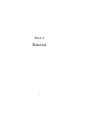
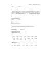
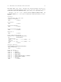
1.2
An Example
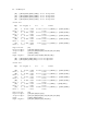
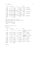
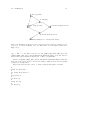
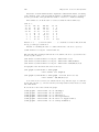
The data of table 1.1 from Reinis̆ et al. (1981) is also used in Edwards & Havránek
(1985).
3
4
Chapter 1. Introduction to CoCo
B
A
No
No
Yes
Yes
No
Yes
F
E
D
C
Negative
<3
<140
No
44
40
112
67
Yes
129
145
12
23
No
35
12
80
33
Yes
109
67
7
9
No
23
32
70
66
Yes
50
80
7
13
No
24
25
73
57
Yes
51
63
7
16
No
5
7
21
9
Yes
9
17
1
4
No
4
3
11
8
Yes
14
17
5
2
No
7
3
14
14
Yes
9
16
2
3
No
4
0
13
11
Yes
5
14
4
4
>140
>3
<140
>140
Positive
<3
<140
>140
>3
<140
>140
A, smoking; B, strenuous mental work; C, strenuous physical work;
D, systolic blood pressure; E, ratio of α to β lipoproteins;
F, family anamnesis of coronary heart disease.
Table 1.1: Risk factors for coronary heart disease.
Start CoCo and give the command SET KEYBOARD On; to indicate that you want
to read data from the keyboard. Then type READ DATA;. CoCo will respond with
the prompt DATA-> indicating that CoCo is expecting data. Declare the table with
Factors A2/B2/C2/D2/E2/F2// and give the keyword Table to tell CoCo that the
data is to be entered in table-form. Then type the 64 cell-counts and end with /.
>keyboard;
Keyboard set ON
>read data;
DATA->Factors A 2 / B 2 / C 2 / D 2 / E 2 / F 2
DATA->Table
DATA-> 44 40 112 67 129 145 12 23
35 12 80
DATA-> 23 32 70 66
50 80
7 13
24 25 73
DATA-> 5 7 21 9
9 17
1 4
4 3 11
DATA-> 7 3 14 14
9 16
2 3
4 0 13
64 cells with 1841 cases read.
Finding all marginals.
>
//
33
57
8
11
109
51
14
5
67
63
17
14
7 9
7 16
5 2
4 4/
The table can also be entered as a list of observations. See chapter 3 for details on
1.2. An Example
5
this and for details on the declaration of factors.
The declaration of factors and the table can be placed on a file, e.g., reinis81.dat:
Factors A 2 /
Table
44 40 112
129 145
12
35 12
80
109 67
7
23 32
70
50 80
7
24 25
73
51 63
7
5
7
21
9 17
1
4
3
11
14 17
5
7
3
14
9 16
2
4
0
13
5 14
4
B 2 / C 2 / D 2/ E 2 / F 2 //
67
23
33
9
66
13
57
16
9
4
8
2
14
3
11
4
This file is then declared to CoCo by SET INPUTFILE DATA reinis81.dat; and
then read by READ DATA; without arguments:
CoCo
in very large
Version 1.3
Compiled with
Copyright (c)
A program for estimation, test and model search
’Co’mplete and ’InCo’mplete ’Co’ntingency tables.
Friday March 17 12:00:00 MET 1995
gcc, a C compiler for Sun4
1991, by Jens Henrik Badsberg
>set inputfile data reinis81.dat;
>read data;
64 cells with 1841 cases read.
Finding all marginals.
>
The declaration of factors and the table or list of cases can be placed on separate
files. See chapter 3. Chapter 3 also describes how to read incomplete tables, group
levels, make data selection and handle missing values in lists of observations.
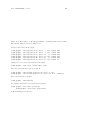
After reading the data any marginal table of observations can be printed with the
command PRINT OBSERVED hseti;, where hseti is a subset of the declared factors. The
asterisk * is an abbreviation of the set containing all factors, so in the following PRINT
OBSERVED ABCDEF.; is equivalent to PRINT OBSERVED *;:
6
Chapter 1. Introduction to CoCo
>print observed ABCDEF.;
[ABCDEF]
C
B
A
1
1
2
1
1
2
2
1
2
1
2
2
2
129 145
109 67
12
7
23
9
1
F
E
D
1
1
1
2
44
35
40
12
112
80
67
33
2
1
2
23
24
32
25
70
73
66
57
50
51
80
63
7
7
13
16
1
1
2
5
4
7
3
21
11
9
8
9
14
17
17
1
5
4
2
2
1
2
7
4
3
0
14
13
14
11
9
5
16
14
2
4
3
4
2
>print observed AB.;
[AB]
A
1
2
B
1
2
522 541
439 339
>
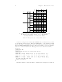
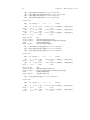
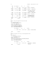
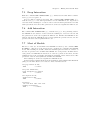
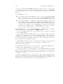
DESCRIBE OBSERVED hseti;, where hseti is a subset of the declared factors, will give
a univariate description of the values in the marginal table. The SET PAGE FORMATS
hline-lengthi hpage-lengthi; is used to make the plot fit into this guide.
#
#
#
#
#
Version 1.3
Friday March 17 12:00:00 MET 1995
Compiled with gcc, a C compiler for Sun4
Compile-time: Mar 17 1995, 13:00:00.
Copyright (c) 1991, by Jens Henrik Badsberg
Licensed to ...
Diary set ON
>read data;
64 cells with 1841 cases read.
Finding all marginals.
TIME:
0.083secs.
1.2. An Example
7
>#
># Change the size of a page to fit into this guide:
>#
>set page formats 72 52;
TIME:
0.000secs.
>#
># Describe the observed counts in the saturated table
># (print also a uniform plot):
>#
>describe table uniform observed * ;
DESCRIBE TABLE:
Observed
NUMBER OF CELLS IN TABLE:
NUMBER OF INVALID CELLS:
NUMBER OF CELLS TO DESCRIBE:
64
0
64
SORTED LIST
0.0000
4.0000
5.0000
9.0000
12.0000
16.0000
24.0000
50.0000
70.0000
145.0000
1.0000
4.0000
7.0000
9.0000
13.0000
16.0000
25.0000
51.0000
73.0000
2.0000
4.0000
7.0000
9.0000
13.0000
17.0000
32.0000
57.0000
80.0000
2.0000
4.0000
7.0000
9.0000
14.0000
17.0000
33.0000
63.0000
80.0000
3.0000
4.0000
7.0000
11.0000
14.0000
21.0000
35.0000
66.0000
109.0000
3.0000
5.0000
7.0000
11.0000
14.0000
23.0000
40.0000
67.0000
112.0000
3.0000
5.0000
8.0000
12.0000
14.0000
23.0000
44.0000
67.0000
129.0000
STATISTICS
NUMBER OF VALUES:
25%:
50%:
75%:
RANK:
RANK:
RANK:
MINIMUM:
MAX RUN:
64
16 VALUE:
32 VALUE:
48 VALUE:
0.0000
5
SUM (X)
:
SUM (1/X) :
PROD (X)
:
SUM (X-MEAN)^2 :
SUM (X-MEAN)^3 :
SUM (X-MEAN)^4 :
7.0000
14.0000
40.0000
MAXIMUM:
MODE:
1841.0000
0.0000
7.096E+04
3.956E+06
4.113E+08
RANK:
RANK:
RANK:
145.0000
4.0000
17 VALUE:
33 VALUE:
49 VALUE:
RANGE:
# < Eps.:
MEAN:
HARMONIC MEAN:
GEOMETRIC MEAN:
VARIANCE:
SKEWNESS:
KURTOSIS:
7.0000
14.0000
44.0000
145.0000
1
28.7656
0.0000
1108.6794
1.6744
5.2282
8
Chapter 1. Introduction to CoCo
UNIFORM PLOT
Unit horizontal: - =
1.00000
0.97500
0.95000
0.92500
0.90000
0.87500
0.85000
0.82500
0.80000
0.77500
0.75000
0.72500
0.70000
0.67500
0.65000
0.62500
0.60000
0.57500
0.55000
0.52500
0.50000
0.47500
0.45000
0.42500
0.40000
0.37500
0.35000
0.32500
0.30000
0.27500
0.25000
0.22500
0.20000
0.17500
0.15000
0.12500
0.10000
0.07500
0.05000
0.02500
0.0E+00
2.5000
!-----------------------------------------------------------!
!
*!
!
*
*
++ !
!
*
*
+
!
!
*
++
!
!
**
+
!
!
*
+
!
!
**
++
!
!
* *
+
!
!
*
++
!
!
* *
+
!
!
*
++
!
!
**
+
!
!
* *
++
!
!
*
+
!
!
2
++
!
!
*
+
!
!
2
+
!
!
2
++
!
!
*
+
!
!
2
++
!
!
*
+
!
!
2
++
!
!
2
+
!
!
*
++
!
!
2
+
!
!
*
+
!
!
2
++
!
!
2
+
!
!
*
++
!
!
2
+
!
!
*
++
!
! 2
+
!
! 2
++
!
! *
+
!
! 2
++
!
! *
+
!
! 2
+
!
! 2 ++
!
! * +
!
!2++
!
!+
!
!+---------+---------+---------+---------+---------+--------!
0.0000
25.0000
50.0000
75.0000 100.0000 125.0000
Observed
1.2. An Example
9
HISTOGRAM
Unit horizontal: * =
Unit vertical:
! =
0.0000
10.0000
20.0000
30.0000
40.0000
50.0000
60.0000
70.0000
80.0000
90.0000
100.0000
110.0000
120.0000
130.0000
140.0000
150.0000
160.0000
->
->
->
->
->
->
->
->
->
->
->
->
->
->
->
->
!
!
!
!
!
!
!
!
!
!
!
!
!
!
!
!
1
10.0000
************
***********************
********
***
***
**
**
*****
**
**
*
*
COUNTS
! Cell
! Number of ! Cumm.
! % of total ! Cumm. %
!
! count
! cells with ! number of ! number of !
!
!
! count
! cells
! cells
!
!
!------------!------------!------------!------------!------------!
!
0 !
1 !
1 !
0.0156 !
0.0156 !
!
1 !
1 !
2 !
0.0156 !
0.0312 !
!
2 !
2 !
4 !
0.0312 !
0.0625 !
!
3 !
3 !
7 !
0.0469 !
0.1094 !
!
4 !
5 !
12 !
0.0781 !
0.1875 !
!
5 !
3 !
15 !
0.0469 !
0.2344 !
!
7 !
5 !
20 !
0.0781 !
0.3125 !
!
8 !
1 !
21 !
0.0156 !
0.3281 !
!
9 !
4 !
25 !
0.0625 !
0.3906 !
!
11 !
2 !
27 !
0.0312 !
0.4219 !
!
. !
. !
. !
. !
. !
!
. !
. !
. !
. !
. !
!
67 !
2 !
56 !
0.0312 !
0.8750 !
!
70 !
1 !
57 !
0.0156 !
0.8906 !
!
73 !
1 !
58 !
0.0156 !
0.9062 !
!
80 !
2 !
60 !
0.0312 !
0.9375 !
!
109 !
1 !
61 !
0.0156 !
0.9531 !
!
112 !
1 !
62 !
0.0156 !
0.9688 !
!
129 !
1 !
63 !
0.0156 !
0.9844 !
!
145 !
1 !
64 !
0.0156 !
1.0000 !
!------------!------------!------------!------------!------------!
10
Chapter 1. Introduction to CoCo
TIME:
0.126secs.
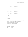
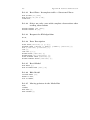
The hierarchical log-linear interaction model described by the generating class hgci
is read by READ MODEL hgci;; for example,
>read model AB,BC.;
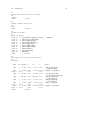
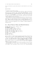
Observed counts, estimated counts, probabilities and residuals (absolute, adjusted,
standard, Freeman-Tukey, etc.) can be printed in tables or described with the commands, e.g., PRINT TABLE Probabilities hseti; and DESCRIBE TABLE Adjusted
Residuals hseti; or the values can be listed or plotted against each other with LIST
hseti; and PLOT hx-value-namei hy-value-namei hseti;. See chapter 4 for details.
>#
># Read model ACE,ADE,BC,F.
>#
>read model ACE,ADE,BC,F. ;
TIME:
0.017secs.
#
# Change the page-size
#
>set page formats 72 36 ;
TIME:
0.000secs.
>#
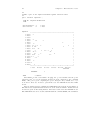
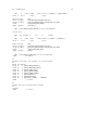
># Describe the adjusted residuals in the marginal table BCDEF.:
>#
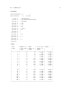
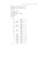
>describe table rankit adjusted BCDEF. ;
DESCRIBE TABLE:
Adjusted
NUMBER OF CELLS IN TABLE:
NUMBER OF INVALID CELLS:
NUMBER OF CELLS TO DESCRIBE:
32
0
32
SORTED LIST
-3.4465
-0.4999
-0.1614
0.7317
1.4399
-2.2064
-0.4912
-0.1219
0.8584
1.7381
-2.1418
-0.4444
-0.0463
0.9000
1.9406
-0.9380
-0.4315
0.1210
0.9719
4.1246
-0.8524
-0.2857
0.1490
1.1956
-0.7695
-0.2795
0.2556
1.2852
-0.6893
-0.2417
0.3147
1.3426
STATISTICS
NUMBER OF VALUES:
25%:
50%:
75%:
RANK:
RANK:
RANK:
32
8 VALUE:
16 VALUE:
24 VALUE:
-0.4999
-0.1219
0.9000
RANK:
RANK:
RANK:
9 VALUE:
17 VALUE:
25 VALUE:
-0.4912
-0.0463
0.9719
1.2. An Example
MINIMUM:
MAX RUN:
11
-3.4465
1
SUM (X)
:
SUM (1/X) :
PROD (X)
:
SUM (X-MEAN)^2 :
SUM (X-MEAN)^3 :
SUM (X-MEAN)^4 :
MAXIMUM:
MODE:
3.3213
-30.8929
-0.0000
58.7837
12.1395
506.5294
4.1246
-
RANGE:
# < Eps.:
MEAN:
HARMONIC MEAN:
GEOMETRIC MEAN:
VARIANCE:
SKEWNESS:
KURTOSIS:
7.5711
0
0.1038
-1.0358
-0.6163
1.8370
0.1524
4.6907
RANKIT PLOT
Unit horizontal: - =
Unit vertical:
! =
2.20000
2.00000
1.80000
1.60000
1.40000
1.20000
1.00000
0.80000
0.60000
0.40000
0.20000
0.0E+00
-0.20000
-0.40000
-0.60000
-0.80000
-1.00000
-1.20000
-1.40000
-1.60000
-1.80000
-2.00000
-2.20000
TIME:
0.1250
0.2000
!--------------------------------------------------------------!
!
++
!
!
++
*!
!
++
!
!
* ++
!
!
*+++
!
!
*++
!
!
**+
!
!
*+*
!
!
2+
!
!
* +*
!
!
2*++
!
!
**+
!
!
2*
!
!
+**
!
!
++2
!
!
++* *
!
!
+++ **
!
!
++
*
!
!
* ++
!
!
*++
!
!
++
!
!*
++
!
!
+++
!
!+---------+---------+---------+---------+---------+---------+-!
-3.5000
-2.2500
-1.0000
0.2500
1.5000
2.7500
Adjusted
0.104secs.
(A histogram is omitted from the above output.)
12
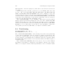
Chapter 1. Introduction to CoCo
>#
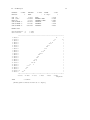
># Make a plot of the adjusted residuals against observed counts
>#
>plot observed adjusted * ;
PLOT OF:
PLOT
Adjusted BY Observed
Unit horizontal: - =
Unit vertical:
! =
2.5000
0.2500
Adjusted
2.5000
2.2500
2.0000
1.7500
1.5000
1.2500
1.0000
0.7500
0.5000
0.2500
0.0000
-0.2500
-0.5000
-0.7500
-1.0000
-1.2500
-1.5000
-1.7500
-2.0000
-2.2500
!-----------------------------------------------------------!
! *
!
!
!
!
!
! 2
!
!
**
*
!
!
*
!
!
2
!
! * * 3 *
*
*
!
! 2 ***
*
!
! ** *
**
*
*!
!
*
*
* 2 *
*
!
! *2 *
**
!
!
**
*
2
!
! *2 2
*
* *
!
!* *
*
!
!
* *
!
!
!
!
*
!
!*
!
!
*
!
!+---------+---------+---------+---------+---------+--------!
0.0000
25.0000
50.0000
75.0000 100.0000 125.0000
Observed
EXCLUDED:
TIME:
0
0.066secs.
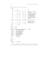
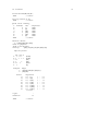
The likelihood ratio test statistic -2log(Q), the χ2 test statistic and the power
divergence 2nI λ for one model under another model is computed by the command
TEST;. The power hλi in computing the power divergence is by default set to 2/3.
CoCo has to know two models to perform the test: the current model and a base
model.
The model first read is both base and current and is given the model number 1.
The first model stays base until another model is declared as base. Additional read
models are given an increasing number. The last read model is the current model.
The current model can be declared as base with the command BASE;. Model number
1.2. An Example
13
hai is named base or current with the commands MAKE BASE hai; and MAKE CURRENT
hai; respectively.
In the example, the model {{ACE},{ADE},{BC},{F}} can be tested against
{{ABCDEF}} by:
>read model *;
>base;
>read model ACE,ADE,BC,F.;
>test;
Test of [[F][BC][ADE][ACE]]
against [[ABCDEF]]
-2log(Q)
Power
X^2
DF.
=
=
=
=
Statistic
62.0779
59.7593
59.9956
P =
P =
P =
Asymptotic
0.0994
0.1396
0.1350
49
/
/
/
/
Adjusted
0.0994
0.1396
0.1350
49
>
The first column of figures is the test statistic, the second is the asymptotic p-values
based on an unadjusted number of degrees of freedom and the third is the p-values
based on an adjusted number of degrees of freedom.
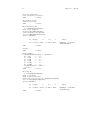
With SET EXACT TEST On; exact test is turned on. The exact test for one decomposable model against another decomposable model containing the model is then
computed by EXACT TEST;:
>set exact test on;
EXACT TEST SET ON
>exact test;
Test of [[F][BC][ADE][ACE]]
against [[ABCDEF]]
-2log(Q)
Power
X^2
DF
>
=
=
=
=
Statistic
62.0779
59.7593
59.9956
P =
P =
P =
Asymptotic
0.0994
0.1396
0.1350
49
/
/
/
/
Adjusted
0.0994
0.1396
0.1350
49
/
/
/
Exact
0.1550
0.1630
0.1570
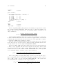
The following is an example of a model-search with the commands BACKWARD;
and FORWARD;. Comments are inserted in the source-file with the character #. The
following is a copy of the diary, edited a little: some blank lines removed, echo of
comments removed, page-breaks removed and inserted:
#
#
#
#
#
Version 1.3
Friday March 17 12:00:00 MET 1995
Compiled with gcc, a C compiler for Sun4
Compile-time: Mar 17 1995, 13:00:00.
Copyright (c) 1991, by Jens Henrik Badsberg
Licensed to ...
14
Chapter 1. Introduction to CoCo
>#
># Set diary on:
>#
>set diary on;
Diary set ON
>#
># Keep the log:
>#
>set keep log;
Keep Log set ON
>#
># Set timer on:
>#
>set timer on;
Timer set ON
TIME:
0.002secs.
>#
># Set the input-file:
>#
>set input data reinis81.dat ;
TIME:
0.003secs.
>#
># Read data
>#
>read data;
64 cells with 1841 cases read.
Finding all marginals.
TIME:
0.025secs.
>#
># Read the saturated model:
>#
>read model *;
TIME:
0.001secs.
>#
># Name this model "current" and then the "current" model "base"
>#
>current;
TIME:
0.001secs.
>base;
TIME:
0.001secs.
1.2. An Example
15
>#
># Choose exact test and
># compute also exact test P-value for Pearson’s chi-spuare:
>#
>set exact test all;
Exact test set ON
Only Exact Deviance set OFF
TIME:
0.001secs.
>#
># Let CoCo decide on the number of tables to generate:
>#
>set number of tables null;
TIME:
0.001secs.
>#
># Ignore non-decomposable models:
>#
>set decomposable mode on;
Decomposable mode set ON
TIME:
0.001secs.
>#
># Do not compute the adjusted number of degrees of freedom:
>#
>set adjusted df off;
Adjusted df set OFF
TIME:
0.001secs.
>#
># Do not compute
>#
>set power lambda
Power Divergence
TIME:
power divergence
null;
not printed
0.002secs.
>#
># Change the size of a page to fit into this guide:
>#
>set page formats 72 256;
TIME:
0.002secs.
>#
># Change the test formats:
>#
>set test formats 8 3 6 4;
TIME:
0.000secs.
16
>#
>#
>#
>#
>#
>#
Chapter 1. Introduction to CoCo
Do a recursive backward-elimination,
where tests are done against the previously accepted model (follow)
and edge exclusions once rejected remain rejected (coherent).
Print only the sorted list of tests (only sorted):
>only
sorted
recursive
coherent
follow
backward;
Sorted list
Edge
DF -2log(Q)
P
[AC]
Exact (
[BC]
Exact (
[AE]
Exact (
[DE]
Exact (
[AD]
Exact (
[AB]
Exact (
[CF]
Exact (
[BF]
Exact (
[AF]
Exact (
[CE]
Exact (
[DF]
Exact (
[EF]
Exact (
[BE]
Exact (
[CD]
Exact (
[BD]
Exact (
16
42.804
1000 )
16 684.989
1000 )
16
40.024
1000 )
16
31.059
1000 )
16
28.724
1000 )
16
22.652
1000 )
16
22.153
100 )
16
22.788
1000 )
16
21.305
100 )
16
18.629
100 )
16
18.345
100 )
16
18.316
200 )
16
17.226
100 )
16
14.808
20 )
16
12.226
20 )
0.0005
0.0000
0.0000
0.0000
0.0010
0.0030
0.0132
0.0310
0.0257
0.0420
0.1232
0.1740
0.1381
0.1800
0.1193
0.1890
0.1668
0.2700
0.2878
0.3700
0.3035
0.3700
0.3052
0.4000
0.3709
0.4600
0.5389
0.6000
0.7293
0.8500
Edge selected:
Rejected edges:
Accepted edges:
Model:
Edges eligible:
X^2
P
41.617 0.0007
0.0000
631.304 0.0000
0.0000
38.762 0.0015
0.0020
30.222 0.0168
0.0230
27.465 0.0363
0.0380
21.213 0.1702
0.1770
20.746 0.1881
0.1400
23.124 0.1102
0.1100
19.710 0.2331
0.2600
17.517 0.3526
0.3800
17.196 0.3728
0.3700
17.820 0.3341
0.3450
16.113 0.4454
0.4600
13.427 0.6422
0.6500
10.985 0.8109
0.9500
Models
R [[ABCDEF]] / [[ABDEF][BCDEF]]
R [[ABCDEF]] / [[ABDEF][ACDEF]]
R [[ABCDEF]] / [[ABCDF][BCDEF]]
R [[ABCDEF]] / [[ABCDF][ABCEF]]
R [[ABCDEF]] / [[ABCEF][BCDEF]]
R [[ABCDEF]] / [[ACDEF][BCDEF]]
R [[ABCDEF]] / [[ABCDE][ABDEF]]
R [[ABCDEF]] / [[ABCDE][ACDEF]]
R [[ABCDEF]] / [[ABCDE][BCDEF]]
R [[ABCDEF]] / [[ABCDF][ABDEF]]
R [[ABCDEF]] / [[ABCDE][ABCEF]]
R [[ABCDEF]] / [[ABCDE][ABCDF]]
R [[ABCDEF]] / [[ABCDF][ACDEF]]
R [[ABCDEF]] / [[ABCEF][ABDEF]]
R [[ABCDEF]] / [[ABCEF][ACDEF]]
[BD]
[[AD][DE][AE][BC][AC]]
[[BD][CD][BE][EF][DF][CE][AF][BF][CF][AB]]
[[ABCEF][ACDEF]]
[[AB][AF][BE][BF][CD][CE][CF][DF][EF]]
1.2. An Example
[AF]
[CE]
[CF]
[EF]
17
[[ABCE][ACDE][BCEF][CDEF]]
[[ABCF][ABEF][ACDF][ADEF]]
[[ABCE][ABEF][ACDE][ADEF]]
[[ABCE][ABCF][ACDE][ACDF]]
is
is
is
is
not
not
not
not
decomposable
decomposable
decomposable
decomposable
Sorted list
Edge
DF -2log(Q)
[AB]
Exact (
[BF]
Exact (
[DF]
Exact (
[BE]
Exact (
[CD]
Exact (
8
15.574
1000 )
8
15.744
200 )
8
11.302
200 )
8
11.364
200 )
8
7.149
100 )
Edge selected:
Rejected edges:
Accepted edges:
Model:
Edges eligible:
[EF]
[AF]
P
0.0484
0.0530
0.0457
0.0850
0.1845
0.1750
0.1812
0.1850
0.5214
0.5600
X^2
P
15.364 0.0519
0.0560
16.733 0.0327
0.0450
11.478 0.1754
0.1550
11.268 0.1863
0.1850
7.067 0.5301
0.5700
Models
R [[ABCEF]] / [[ACEF][BCEF]]
R [[ABCEF]] / [[ABCE][ACEF]]
R [[ACDEF]] / [[ACDE][ACEF]]
R [[ABCEF]] / [[ABCF][ACEF]]
R [[ACDEF]] / [[ACEF][ADEF]]
[CD]
[[AD][DE][AE][BC][AC]]
[[BD][CD][BE][EF][DF][CE][AF][BF][CF][AB]]
[[ABCEF][ADEF]]
[[EF][DF][CF][CE][BF][BE][AF][AB]]
[[ABCE][ABCF][ADE][ADF]] is not decomposable
[[ABCE][ADE][BCEF][DEF]] is not decomposable
Sorted list
Edge
DF -2log(Q)
[AB]
Exact (
[BF]
Exact (
[CF]
Exact (
[BE]
Exact (
[DF]
Exact (
[CE]
Exact (
8
15.574
1000 )
8
15.744
200 )
8
12.237
100 )
8
11.364
200 )
4
6.368
200 )
8
12.735
200 )
Edge selected:
Rejected edges:
Accepted edges:
Model:
Edges eligible:
P
0.0484
0.0530
0.0457
0.0850
0.1403
0.1300
0.1812
0.1850
0.1733
0.1950
0.1207
0.2000
X^2
P
15.364 0.0519
0.0560
16.733 0.0327
0.0450
11.687 0.1651
0.1300
11.268 0.1863
0.1850
6.583 0.1596
0.1750
12.666 0.1233
0.1950
Models
R [[ABCEF]] / [[ACEF][BCEF]]
R [[ABCEF]] / [[ABCE][ACEF]]
R [[ABCEF]] / [[ABCE][ABEF]]
R [[ABCEF]] / [[ABCF][ACEF]]
R [[ADEF]] / [[ADE][AEF]]
R [[ABCEF]] / [[ABCF][ABEF]]
[CE]
[[AD][DE][AE][BC][AC]]
[[BD][CD][BE][EF][DF][CE][AF][BF][CF][AB]]
[[ABCF][ABEF][ADEF]]
[[AB][AF][BE][BF][CF][DF][EF]]
18
Chapter 1. Introduction to CoCo
[AB]
[AF]
[BF]
[EF]
[[ACF][ADEF][BCF][BEF]] is not decomposable
[[ABC][ABE][ADE][BCF][BEF][DEF]] is not decomposable
[[ABC][ABE][ACF][ADEF]] is not decomposable
[[ABCF][ABE][ADE][ADF]] is not decomposable
Sorted list
Edge
DF -2log(Q)
[BE]
Exact (
[CF]
Exact (
[DF]
Exact (
4
21.159
1000 )
4
7.018
1000 )
4
6.368
200 )
Edge selected:
Rejected edges:
Accepted edges:
Model:
Edges eligible:
[BF]
[AF]
[AB]
P
0.0003
0.0000
0.1349
0.1320
0.1733
0.1950
X^2
P
21.168 0.0003
0.0000
7.459 0.1135
0.0930
6.583 0.1596
0.1750
Models
R [[ABEF]] / [[ABF][AEF]]
R [[ABCF]] / [[ABC][ABF]]
R [[ADEF]] / [[ADE][AEF]]
[DF]
[[BE][AD][DE][AE][BC][AC]]
[[BD][CD][BE][EF][DF][CE][AF][BF][CF][AB]]
[[ABCF][ABEF][ADE]]
[[EF][CF][BF][AF][AB]]
[[ABC][ABE][ACF][ADE][AEF]] is not decomposable
[[ABC][ABE][ADE][BCF][BEF]] is not decomposable
[[ACF][ADE][AEF][BCF][BEF]] is not decomposable
Sorted list
Edge
[CF]
Exact (
[EF]
Exact (
DF -2log(Q)
4
1000
4
100
7.018
)
3.951
)
Edge selected:
Rejected edges:
Accepted edges:
Model:
Edges eligible:
[AB]
P
0.1349
0.1320
0.4127
0.3900
X^2
P
7.459 0.1135
0.0930
4.075 0.3959
0.3800
Models
R [[ABCF]] / [[ABC][ABF]]
R [[ABEF]] / [[ABE][ABF]]
[EF]
[[BE][AD][DE][AE][BC][AC]]
[[BD][CD][BE][EF][DF][CE][AF][BF][CF][AB]]
[[ABCF][ABE][ADE]]
[[AB][AF][BF][CF]]
[[ACF][ADE][BCF][BE]] is not decomposable
Sorted list
Edge
DF -2log(Q)
[BF]
Exact (
[AF]
Exact (
4
11.151
1000 )
4
7.386
200 )
P
0.0249
0.0270
0.1169
0.1200
X^2
P
13.302 0.0099
0.0060
7.336 0.1192
0.1200
Models
R [[ABCF]] / [[ABC][ACF]]
R [[ABCF]] / [[ABC][BCF]]
1.2. An Example
[CF]
Exact (
4
7.018 0.1349
1000 )
0.1320
Edge selected:
Rejected edges:
Accepted edges:
Model:
Edges eligible:
[AB]
19
7.459 0.1135
0.0930
R [[ABCF]] / [[ABC][ABF]]
[CF]
[[BF][BE][AD][DE][AE][BC][AC]]
[[BD][CD][BE][EF][DF][CE][AF][BF][CF][AB]]
[[ABC][ABE][ABF][ADE]]
[[AF][AB]]
[[AC][ADE][AF][BC][BE][BF]] is not decomposable
Sorted list
Edge
[AF]
Exact (
DF -2log(Q)
2
2.658 0.2647
100 )
0.2300
Edge selected:
Rejected edges:
Accepted edges:
Model:
Edges eligible:
[AB]
TIME:
P
X^2
P
2.648 0.2661
0.2300
Models
R [[ABF]] / [[AB][BF]]
[AF]
[[BF][BE][AD][DE][AE][BC][AC]]
[[BD][CD][BE][EF][DF][CE][AF][BF][CF][AB]]
[[ABC][ABE][ADE][BF]]
[[AB]]
[[AC][ADE][BC][BE][BF]] is not decomposable
12.096secs.
>#
># Print all models, the sequence of accepted models:
>#
>print all models;
Model no.
8 [[ABC][ABE][ADE][BF]]
Model no.
7 [[ABC][ABE][ABF][ADE]]
Model no.
6 [[ABCF][ABE][ADE]]
Model no.
5 [[ABCF][ABEF][ADE]]
Model no.
4 [[ABCF][ABEF][ADEF]]
Model no.
3 [[ABCEF][ADEF]]
Model no.
2 [[ABCEF][ACDEF]]
Model no.
1 [[ABCDEF]] /BASE/
/CURRENT/
TIME:
0.005secs.
>#
># Name the last accepted model "current"
>#
>current;
TIME:
0.001secs.
20
Chapter 1. Introduction to CoCo
>#
># Name "current" model "base"
>#
>base;
TIME:
0.000secs.
>#
># Print all models:
>#
>print all models;
Model no.
8 [[ABC][ABE][ADE][BF]] /BASE/
Model no.
7 [[ABC][ABE][ABF][ADE]]
Model no.
6 [[ABCF][ABE][ADE]]
Model no.
5 [[ABCF][ABEF][ADE]]
Model no.
4 [[ABCF][ABEF][ADEF]]
Model no.
3 [[ABCEF][ADEF]]
Model no.
2 [[ABCEF][ACDEF]]
Model no.
1 [[ABCDEF]]
TIME:
0.005secs.
/CURRENT/
>#
># Can an edge rejected by ’coherence’ now be rejected:
>#
>backward;
Edge
DF -2log(Q)
P
X^2
P
Models
[AB] [[AC][ADE][BC][BE][BF]] is not decomposable
[AC]
2
23.805 0.0000
23.929 0.0000
[[ABC]] / [[AB][BC]]
Exact (
1000 )
0.0000
0.0000
[AD]
2
16.542 0.0003
16.427 0.0003
[[ADE]] / [[AE][DE]]
Exact (
1000 )
0.0000
0.0000
[AE] [[ABC][AD][BE][BF][DE]] is not decomposable
[BC]
2 682.296 0.0000 631.416 0.0000
[[ABC]] / [[AB][AC]]
Exact (
1000 )
0.0000
0.0000
[BE]
2
20.929 0.0000
20.930 0.0000
[[ABE]] / [[AB][AE]]
Exact (
1000 )
0.0000
0.0000
[BF]
1
4.732 0.0296
4.772 0.0289
[[BF]] / [[B][F]]
Exact (
1000 )
0.0300
0.0300
[DE]
2
18.319 0.0001
18.298 0.0001
[[ADE]] / [[AD][AE]]
Exact (
1000 )
0.0000
0.0000
TIME:
1.561secs.
>#
># Did accept wrong edges in the start:
>#
>forward;
1.2. An Example
Edge
DF -2log(Q)
21
P
X^2
P
Models
[AF]
2
2.658 0.2647
2.648 0.2661 R [[ABF]] / [[AB][BF]]
Exact (
100 )
0.2300
0.2300
[BD]
4
2.504 0.6439
2.502 0.6443
[[ABDE]] / [[ABE][ADE]]
Exact (
20 )
0.7000
0.7000
[CD] [[ABC][ABE][ACD][ADE][BF]] is not decomposable
[CE]
4
7.516 0.1110
7.602 0.1073
[[ABCE]] / [[ABC][ABE]]
Exact (
1000 )
0.1010
0.0940
[CF]
2
2.290 0.3182
2.426 0.2974
[[BCF]] / [[BC][BF]]
Exact (
100 )
0.3300
0.3100
[DF] [[ABC][ABE][ADE][BF][DF]] is not decomposable
[EF]
2
2.405 0.3004
2.427 0.2972
[[BEF]] / [[BE][BF]]
Exact (
100 )
0.2700
0.2700
TIME:
0.523secs.
>#
># Set DecomposableMode off to compute
># asymptotic P-values for non-decomposable models:
>#
>set decomposable mode off;
Decomposable mode set OFF
TIME:
0.001secs.
>#
># Compute asymptotic P-values
>#
>backward;
Edge
[AB]
DF -2log(Q)
3
P
6.177 0.1033
X^2
P
6.162 0.1040
[AC]
Exact (
[AD]
Exact (
[AE]
2
23.805
1000 )
2
16.542
1000 )
3
26.077
0.0000
0.0000
0.0003
0.0000
0.0000
23.929 0.0000
0.0000
16.427 0.0003
0.0000
25.991 0.0000
[BC]
Exact (
[BE]
Exact (
[BF]
Exact (
[DE]
Exact (
TIME:
2 682.296 0.0000
1000 )
0.0000
2
20.929 0.0000
1000 )
0.0000
1
4.732 0.0296
1000 )
0.0300
2
18.319 0.0001
1000 )
0.0000
0.076secs.
631.416 0.0000
0.0000
20.930 0.0000
0.0000
4.772 0.0289
0.0300
18.298 0.0001
0.0000
>forward;
Models
[[ABE][ABC]] / [[BE][BC]
[AE][AC]]
R [[ABC]] / [[AB][BC]]
R [[ADE]] / [[AE][DE]]
[[ADE][ABE]] / [[DE][BE]
[AD][AB]]
R [[ABC]] / [[AB][AC]]
R [[ABE]] / [[AB][AE]]
R [[BF]] / [[B][F]]
R [[ADE]] / [[AD][AE]]
22
Chapter 1. Introduction to CoCo
Edge
DF -2log(Q)
P
X^2
P
[AF]
Exact (
[BD]
Exact (
[CD]
2
2.658
100 )
4
2.504
20 )
2
1.084
0.2647
0.2300
0.6439
0.7000
0.5817
2.648 0.2661
0.2300
2.502 0.6443
0.7000
1.084 0.5817
[CE]
Exact (
[CF]
Exact (
[DF]
4
1000
2
100
1
0.1110
0.1010
0.3182
0.3300
0.3045
7.602 0.1073
0.0940
2.426 0.2974
0.3100
1.059 0.3035
[EF]
Exact (
TIME:
2
2.405 0.3004
100 )
0.2700
0.072secs.
2.427 0.2972
0.2700
7.516
)
2.290
)
1.054
Models
R [[ABF]] / [[AB][BF]]
R [[ABDE]] / [[ABE][ADE]]
[[ABC][ABE][ACD][ADE]]
/ [[ABC][ABE][ADE]]
R [[ABCE]] / [[ABC][ABE]]
R [[BCF]] / [[BC][BF]]
[[ABE][ADE][BF][DF]]
/ [[ABE][ADE][BF]]
R [[BEF]] / [[BE][BF]]
>#
># Try to drop the significant interaction ABC:
>#
>drop interaction ABC.;
9: [[BF][BC][AC][ABE][ADE]]
Model is not graphical
Cliques:[[ABC][ABE][ADE][BF]]
2-Section Graph is decomposable
Test of [[BF][BC][AC][ABE][ADE]]
against [[ABC][ABE][ADE][BF]]
DF -2log(Q)
1
TIME:
P
5.986 0.0144
X^2
P
5.951 0.0147
Models
[[ABC]] / [[BC][AC][AB]]
0.026secs.
>#
># Drop the edge AB, and accept a non-decomposable model:
>#
>drop edge AB.;
10: [[AC][ADE][BC][BE][BF]]
Model is graphical
Graph is not decomposable
Generating class for Fill In: [[ACE][ADE][BCE][BF]]
Test of [[AC][ADE][BC][BE][BF]]
against [[ABC][ABE][ADE][BF]]
DF -2log(Q)
3
TIME:
P
6.177 0.1033
0.032secs.
X^2
P
6.162 0.1040
Models
[[ABE][ABC]] / [[BE][BC]
[AE][AC]]
1.2. An Example
23
>#
># Name the last accepted model "current"
>#
>current;
TIME:
0.001secs.
>#
># Name "current" model "base"
>#
>base;
TIME:
0.001secs.
>#
># Print all models:
>#
>print all models;
Model no. 10 [[AC][ADE][BC][BE][BF]] /BASE/
Model no.
9 [[BF][BC][AC][ABE][ADE]]
Model no.
8 [[ABC][ABE][ADE][BF]]
Model no.
7 [[ABC][ABE][ABF][ADE]]
Model no.
6 [[ABCF][ABE][ADE]]
Model no.
5 [[ABCF][ABEF][ADE]]
Model no.
4 [[ABCF][ABEF][ADEF]]
Model no.
3 [[ABCEF][ADEF]]
Model no.
2 [[ABCEF][ACDEF]]
Model no.
1 [[ABCDEF]]
TIME:
0.006secs.
/CURRENT/
>#
># No edges can be removed from this model:
>#
>backward;
Edge
[AC]
[AD]
Exact (
[AE]
DF -2log(Q)
1
P
X^2
P
30.292 0.0000
30.211 0.0000
2
16.542 0.0003
1000 )
0.0000
2
25.887 0.0000
16.427 0.0003
0.0000
25.828 0.0000
[BC]
1
688.782 0.0000
638.896 0.0000
[BE]
1
20.740 0.0000
20.767 0.0000
1
4.732 0.0296
1000 )
0.0300
2
18.319 0.0001
1000 )
0.0000
0.135secs.
4.772 0.0289
0.0300
18.298 0.0001
0.0000
[BF]
Exact (
[DE]
Exact (
TIME:
Models
[[BE][BC][AE][AC]]
/ [[BE][BC][AE]]
R [[ADE]] / [[AE][DE]]
[[AC][ADE][BC][BE]]
/ [[AC][AD][BC][BE][DE]]
[[BE][BC][AE][AC]]
/ [[BE][AE][AC]]
[[BE][BC][AE][AC]]
/ [[BC][AE][AC]]
[[BF]] / [[B][F]]
R [[ADE]] / [[AD][AE]]
24
Chapter 1. Introduction to CoCo
>#
># No edges should be added to the found model:
>#
>forward;
Edge
DF -2log(Q)
P
X^2
P
[AB]
3
6.177 0.1033
6.162 0.1040
[AF]
1
1.388 0.2388
1.389 0.2385
[BD]
2
1.397 0.4974
1.396 0.4976
[CD]
2
1.082 0.5823
1.082 0.5823
[CE]
3
7.365 0.0611
7.456 0.0587
[CF]
Exact (
[DF]
2
2.290 0.3182
100 )
0.3300
1
1.057 0.3038
2.426 0.2974
0.3100
1.062 0.3027
[EF]
Exact (
TIME:
2
2.427 0.2972
0.2700
2.405 0.3004
100 )
0.2700
0.214secs.
>#
># Print all models:
>#
>print all models;
Model no. 10 [[AC][ADE][BC][BE][BF]] /BASE/
Model no.
9 [[BF][BC][AC][ABE][ADE]]
Model no.
8 [[ABC][ABE][ADE][BF]]
Model no.
7 [[ABC][ABE][ABF][ADE]]
Model no.
6 [[ABCF][ABE][ADE]]
Model no.
5 [[ABCF][ABEF][ADE]]
Model no.
4 [[ABCF][ABEF][ADEF]]
Model no.
3 [[ABCEF][ADEF]]
Model no.
2 [[ABCEF][ACDEF]]
Model no.
1 [[ABCDEF]]
TIME:
0.007secs.
>#
># Exit CoCo
>#
>quit;
TIME:
TOTAL TIME:
Models
[[ABE][ABC]] / [[BE][BC]
[AE][AC]]
[[AC][AE][AF][BC][BE][BF]]
/ [[AC][AE][BC][BE][BF]]
[[AC][ADE][BC][BDE]]
/ [[AC][ADE][BC][BE]]
[[ACD][ADE][BC][BE]]
/ [[AC][ADE][BC][BE]]
[[BCE][ACE]] / [[BE][BC]
[AE][AC]]
[[BCF]] / [[BC][BF]]
[[DF][BF][BE][BC]
[ADE][AC]] / [[BF][BE]
[BC][ADE][AC]]
[[BEF]] / [[BE][BF]]
/CURRENT/
0.002secs.
15.017secs.
The model {{ADE},{AC},{BC},{BE},{BF}} found by coherent backward elimination with exact and local tests on the data from Reinis̆ et al. (1981) adds the
1.2. An Example
25
D: Blood pressure
w
Q
Q
Q
Q
Q A: Smoking
Qw
b
b
b
b
b
of lipoproteins
C: Strenuous physical work
E: Ratio
b
bw
w
H
"
HH
"
"
HH
"
"
H
"
HH
w"
B: Strenuous mental work
w
F: Family anamnesi of coronary heart disease
Figure 1.1: A final model from recursive coherent backward elimination with local and
exact tests on data from Reinis et al. 81. The TeX-code of the figure is written by
Xlisp+CoCo.
edge < BF > to the first of the two models {{ADE},{AC},{BC},{BE},{F}} and
{{ACE},{ADE},{BC},{F}} found in Edwards & Havránek (1985). Note also that we
in the search observed that the interaction < ABC > is significant.
The model {{ACE},{ADE},{BC},{F}} from Edwards & Havránek (1985) will in the
next part of the guide often be used as an example. This model is selected mainly
because it is decomposable.
The log-file after the run of CoCo to make output in this chapter looks like:
#
# Name the diary-file:
#
set output diary diary.2 ;
#
# Set diary on:
#
set diary on;
#
# Keep the log:
#
set keep log;
26
Chapter 1. Introduction to CoCo
#
# Set timer on:
#
set timer on;
#
# Set the input-file:
#
set input data reinis81.dat ;
#
# Read data
#
read data;
#Data: Factors A2/B2/C2/D2/E2/F2//
#Data:
#Data: Table
#Data: 44 40 112 67
#Data: 129 145
12 23
#Data: 35 12
80 33
#Data: 109 67
7
9
#Data: 23 32
70 66
#Data: 50 80
7 13
#Data: 24 25
73 57
#Data: 51 63
7 16
#Data:
5
7
21
9
#Data:
9 17
1
4
#Data:
4
3
11
8
#Data: 14 17
5
2
#Data:
7
3
14 14
#Data:
9 16
2
3
#Data:
4
0
13 11
#Data:
5 14
4
4
#
# Change the print-width used when printing tables:
#
set table formats 5 2 2 2;
#
# Print counts in the full table:
#
print observed ABCDEF.;
#
# Print counts in the marginal table AB:
#
print observed AB.;
#
# Print the total count:
#
print observed .;
#
# Change the size of a page to fit into this guide:
#
set page formats 72 52;
1.2. An Example
>#
># Describe the observed counts in the saturated table
># (print also a uniform plot):
>#
>describe table uniform observed * ;
#
# Read model ACE,ADE,BC,F.
#
read model ACE,ADE,BC,F.;
#
# Change the page-size
#
set page formats 72 36;
#
# Describe the adjusted residuals in the marginal table BCDEF.
# Print a ‘rankit’-plot:
#
describe table rankit adjusted BCDEF.;
#
# Make a plot of the adjusted residuals against observed counts
#
plot observed adjusted *;
#
# Read the saturated model:
#
read model *;
#
# Name this model "current" and then the "current" model "base"
#
current;
base;
#
# Choose exact test and
# compute also exact test P-value for Pearson’s chi-spuare:
#
set exact test all;
#
# Let CoCo decide on the number of tables to generate:
#
set number of tables null;
#
# Ignore non-decomposable models:
#
set decomposable mode on;
#
# Do not compute the adjusted number of degrees of freedom:
#
set adjusted df off;
27
28
Chapter 1. Introduction to CoCo
#
# Do not compute power divergence
#
set power lambda null;
#
# Change the size of a page to fit into this guide:
#
set page formats 72 256;
#
# Change the test formats:
#
set test formats 8 3 6 4;
#
# Do a recursive backward-elimination,
# where tests are done against the previously accepted model (follow)
# and edge exclusions once rejected remain rejected (coherent).
# Print only the sorted list of tests (only sorted):
#
only sorted recursive coherent follow backward;
#
# Print all models, the sequence of accepted models:
#
print all models;
#
# Name the last accepted model "current"
#
current;
#
# Name "current" model "base"
#
base;
#
# Print all models:
#
print all models;
#
# Can an edge rejected by ’coherence’ now be rejected:
#
backward;
#
# Did accept wrong edges in the start:
#
forward;
#
# Set DecomposableMode off to compute
# asymptotic P-values for non-decomposable models:
#
set decomposable mode off;
1.2. An Example
29
#
# Compute asymptotic P-values
#
backward;
#
# Compute asymptotic P-values
#
forward;
#
# Try to drop the significant interaction ABC:
#
drop interaction ABC.;
#
# Drop the edge AB, and accept a non-decomposable model:
#
drop edge AB.;
#
# Name the last accepted model "current"
#
current;
#
# Name "current" model "base"
#
base;
#
# Print all models:
#
print all models;
#
# No edges can be removed from this model:
#
backward;
#
# No edges should be added to the found model:
#
forward;
#
# Print all models:
#
print all models;
#
# Exit CoCo
#
quit;
It might be read as input to CoCo by coco < log or the command SOURCE log;
in CoCo.
Part II
User’s Manual
30
Chapter 2
Commands
Command-names in this guide are written in upper-case, like in the command HELP;.
Arguments to CoCo-commands are capitalized, if they are keywords, like in the command SET DIARY [ On | Off ]; or, if they are numbers, names, sets, models, etc.
surrounded by h and i, like in MENU NUMBER hai;.
Keywords and arguments surrounded by [ and ] are optional. If keywords are
surrounded by [ and ] and separated by | either one of the keywords can be given.
If keywords or arguments are surrounded by { and } and separated by | one of the
keywords or arguments must be given.
When reading commands, CoCo does not distinguish between lower and uppercase letters. But note that CoCo distinguishes between lower and upper-case letters
when reading factor names. Several commands separated by ; can be entered on the
same line. A command consisting of more than one word can be divided between two
lines with &.
The current version of CoCo only uses the first 4 characters of each word of a
command name to recognize the command. Commands do not have to be ended by
the character ;. EndOfLine, “Return”, works as well.
2.1
Online HELP
HELP [ hcommand-namei | habbreviationi ];
MENU NUMBER hai;
NEXT MENU;
CURRENT MENU;
PREVIOUS MENU;
An introduction to CoCo is given by the command HELP; without any arguments.
The command HELP; can be given a command-name as an argument: The command
HELP hcommand-namei; will print the full command-name with arguments, and a
description of the command with name hcommand-namei is printed (when this description is entered in the help-file). HELP help; will give a description of how to
use “help”.
32
2.2. Comments
33
If only the beginning of a command-name is given to the help-command, HELP
hstart of command-namei;, then CoCo will show expected continuation of the beginning of command-names, e.g., HELP read; or HELP set;, and some documentation
for that beginning might be printed.
HELP hvalue-namei; will give documentation for the table-value hvalue-namei.
HELP hkeyword i; is used to print documentation for special topics like limits, overlays,
data, etc., See HELP help;.
MENU NUMBER 0; will print a quick-reference-card. With MENU NUMBER hai;, NEXT
MENU;, CURRENT MENU;, PREVIOUS MENU; it is possible to step through the quickreference-card.
If a command is removed from CoCo, then HELP hcommand-namei; will not be
able to reach help information on how the command is replaced. See HELP help; or
HELP removed;.
2.2
Comments
If # is the first character of a command, then characters from # to ; or end of line are
skipped.
2.3
Make, Delete and Print Alias
PRINT ALIAS { hcommand-namei | habbreviationi };
MAKE ALIAS hcommand-namei habbreviationi;
DELETE ALIAS habbreviationi;
Abbreviations for commands with long names can be seen with the command PRINT ALIAS hcommand-namei;. The command HELP habbreviationi; will
print the full command-name with arguments for the command with abbreviation
habbreviationi. New abbreviations can be declared with the command MAKE ALIAS
hcommand-namei habbreviationi;. An abbreviation is deleted with DELETE ALIAS
habbreviationi;.
The author uses the following abbreviations:
make
make
make
make
make
make
make
make
make
make
make
alias
alias
alias
alias
alias
alias
alias
alias
alias
alias
alias
quit
end
set inputfile data
set outputfile diary
set outputfile report
read data
read specification
read observations
read model
print formula
print all models
end ;
e ;
sid ;
sod ;
sor ;
rd ;
rs ;
ro ;
rm ;
pf ;
pam ;
These abbreviations can be placed on the file, e.g., my.alias, and read by the
command SOURCE hfile-namei;: SOURCE my.alias;. See also the next section about
34
Chapter 2. Commands
the local parser. The file .cocorc (COCO.SRC under DOS) is read, when CoCo is
started. See also the chapter 11 about source files.
2.4
Reading a Local Parser
READ LOCAL PARSER;
If you are running a public CoCo on workstations and declaring new abbreviations,
a local version of the parser-table is generated in the current directory. Next time
you start CoCo up in that directory, the local version of the parser table with your
abbreviations can be read in with READ LOCAL PARSER;.
The following two commands are of no interest to the normal user:
INIT PARSER;
NO ACTION;
INIT PARSER; is used by the author to create a new parser-table from the file
INIT.TAB. With the command NO ACTION; CoCo enters a mode, where commands
are read, but no action is performed. Exit this mode by END;.
2.5
Sets and Models
A set is entered as a list of factor names enclosed in sharp parentheses; e.g., the set
with the three variables A, B and C is entered as
[ABC]
A model (generating class, e.g., in the command READ MODEL hgci;) is entered
as a list of sets enclosed in sharp parentheses; for example, the model with the two
generators <AB> and <BC> is entered as
[[AB][BC]]
A shorter form can be used. Comma (,) ends sets whereas period (.) ends both
sets and generating classes so the set above set with the three variables A, B and C can
be also be entered as
ABC.
and the above model can be entered as
AB,BC.
EndOfLine, “Return”, ends sets, generating classes and sets of generating classes
unless the EndOfLine is presided by the character &.
The asterisk * is an abbreviation for the set containing all declared factors and
for the saturated model. Period (., with no factors preceding) is an abbreviation for
the model with only main-effects. The uniform model (model with no effects) can be
entered as ; or [[]].
2.6. Pausing and Front End Processor: History Mechanism
2.5.1
35
Variable names of length longer than one character
If variable names longer than one character are used, then the first character of each
name is :, and sets are entered as, e.g.,
[:Sex:Smoking:Drinking]
or
:Sex:Smoking:Drinking.
and models can be entered as, e.g.,
[[:Sex:Smoking][:Smoking:Drinking]]
or
:Sex:Smoking,:Smoking:Drinking.
2.6
Pausing and Front End Processor:
Mechanism
History
No history-mechanism is implemented in CoCo. On Unix: Use ‘fep’ (If not available
on your system, get your system administrator to install it), or run CoCo as a subprocess in ‘emacs’. On DOS: use the F3-key.
SET PAUSE [ On | Off ];
SET PAGING LENGTH hnumber of linesi;
At some commands, and especially on some fast machines, it has become a problem
to reach to read output from CoCo before it scrolls out of the top of the screen.
With Pausing set on by SET PAUSE [ On | Off ]; (Default: Off) the output is
paused for each written 22 lines (after last NewPage), if EndOfLine is found after the
total command is read by CoCo. E.g., if Pausing is on, then CoCo will pause for each
printed 22 lines after STATUS;. If Pausing is on, then CoCo will not pause during the
status command, if STATUS;; or STATUS; READ MODEL A,B.; is entered. The next
22 lines are printed by pressing “Return”. If a ; is entered when pausing, then the
command will finish without pausing. The number of lines to print between pausing
are set by SET PAGING LENGTH hnumber of linesi; (Default: 22).
Note that not only printing but also computation in CoCo are paused. It is not
recommended to pipe the output from CoCo into pagers like ‘more’ or ‘less’ since you
will not see entered characters to CoCo before you have typed ‘return’. Use ‘cmdtool’,
run CoCo as a sub-process in ‘emacs’, use Control-S and Control-Q or set the diary
on, and use some ‘pager’ on the diary.
A log of the CoCo-session is kept. Unless you use the command SET KEEP LOG On;
or change the LogFileName, the LogFile is removed on Unix when CoCo terminates
normally. See chapter 11 about the LogFile and use the command STATUS Files;
to see default file-names.
36
2.7
Chapter 2. Commands
Print-formats, Tests, Diary, Source, Sink, Log,
etc.
See chapter 11: Options.
2.8
Interrupts
On Unix a Control-C will terminate the IPS-algorithm and the computation of an
exact test. Control-\ or two close Control-C’s will terminate the EM-algorithm, factorization of a test, a BACKWARD;-command , a FORWARD;-command or the computation of a dual in the EH-procedure. See section 11.7: “Interrupts” in chapter 11:
“Miscellaneous Options for ...” for how to set interrupts off.
Chapter 3
Reading Data
The command READ DATA; is used to read observations and specifications of factors
from input or from a file.
3.1
Keyboard and Files
SET KEYBOARD [ On | Off ];
SET INPUTFILE DATA hfile-namei;
SET INPUTFILE SPECIFICATION hfile-namei;
SET INPUTFILE OBSERVATIONS hfile-namei;
READ DATA [ hspecificationi hobservationsi ];
READ SPECIFICATION [ hspecificationi ];
READ FACTORS [ hfactor-listi ];
READ NAMES [ hname-listi ];
READ OBSERVATIONS [ hobservationsi ];
READ TABLE [ htablei ];
READ LIST [ hlist of casesi ];
The data consists of two parts: specification and observations. The specification is
the definition of variables and table. The observations are the cell counts in the table.
Data can either be read from keyboard or file. This is controlled by the command SET
KEYBOARD [ On | Off ];. The following sections will describe how the specification
and observations have to be formatted.
When reading from file, the file with data (specification and observations) is named
(and reset) with the command SET INPUTFILE DATA hfile-namei;. If specification
and observations are not in the same file, the two files are named and reset with SET
INPUTFILE SPECIFICATION hfile-namei; and SET INPUTFILE OBSERVATIONS hfilenamei;.
After naming files, the specification and observations are read with READ DATA;
without arguments. If data are read from key-board, the specification and observations
are expected as arguments to READ DATA [ hspecificationi hobservationsi ];.
37
38
Chapter 3. Reading Data
If data selection is to be done, it has to be declared between reading specification and observations, so READ DATA [ hspecificationi hobservationsi ]; has to be
divided in to the two actions READ SPECIFICATION [ hspecificationi ]; and READ
OBSERVATIONS [ hobservationsi ]; See section 3.8 on data selection.
The command READ LIST [ hlist of casesi ]; is the same command as READ
OBSERVATIONS [ hobservationsi ]; except that the key-word LIST; is not expected.
Analogous to READ NAMES [ hname-listi ];, READ FACTORS [ hfactor-listi ]; and
READ TABLE [ htablei ];. On the key-words Names, List, Factors and Table, see
the following sections.
Specifications and observations are defaults read from the file COCO.DAT in the
home directory for CoCo.
SET DATASTRUCTURE { All | Necessary | File | Large };
SET LARGE [ On | Off ];
SET SORTED [ On | Off ];
These commands control the selected data structure, see the chapter 11 “Options”.
3.2
Specification
The specification declares the number of factors, order of factors and name and number
of levels (non-missing and missing levels) for each factor. Factor-names in CoCo consist
either all of a single character, or names of any length can be used. If factor-names
consist of only a single character, then the name can be any character except slash
(/). E.g., a .. z, A .. Z, 0 .. 9, (and ?, !, @, $, #, %, ∧, , -, +, =, |, \, ∼, ‘, ’
and "). (Some of the special characters may be reserved in later versions of CoCo.)
Note that CoCo distinguishes between lower-case and upper-case letters when reading
factor names. The characters #, *, ,, ., ;, :, /, and parentheses ((, ), [, ], <, >,
{ and } ) can be used as factor names, but should not, since it would cause trouble
when reading sets and models.
If names consisting of more than one character are to be used, then all names must
be declared with : as the first character.
The specification starts either with the key-word Factors or with the key-word
Names:
3.2.1
Factor by Factor: Factors
If Factors is found, a list of items separated by / and ended by // is expected. The
number of items defines the number of factors, and the order of the items defines the
order of factors used when reading data. Each item consists of a name (a character),
number of non-missing levels (an integer) and an optional number of levels to be interpreted as missing values (see section 3.9 Missing Values: Incomplete observations);
for example,
Factors A 2 / B 2 / C 2 1 //
or
Factors :Sex 2 / :Smoking 2 / :Drinking 2 1 //
3.3. Ordinal Variables
3.2.2
39
Attributes one by one: Names
These specification could also be entered as
Names A B C / 2 2 2 / 0 0 1
and
Names :Sex :Smoking :Drinking / 2 2 2 / 0 0 1
respectively.
After the key-word Names a list of characters giving names and order of factors is
expected. Then a list of integers giving number of non-missing levels for each factor is
expected. An optional list of number of levels for each factor to be marked as missing
can be entered. If this list is not entered, end the list of numbers of non-missing levels
with //; for example
Names A B C / 2 2 2 //
Factor-levels are integers from 1 up to the total number of levels (number of nonmissing levels plus the number of levels marked as missing).
New users are often confused by the above two ways of declaring the variables.
The form Factors is useful to specify the factors one by one. Names is useful if the
data is entered as a list. The names, number of levels and number of levels to marked
as missing can then be written as headings to the columns of levels for each factor.
The form Names is also used when defining a table from S-Plus or XLISP-STAT, see
chapter 12.
Use STATUS Specification; to see the entered specification.
3.3
Ordinal Variables
SET ORDINAL hseti;
With this command the factors of the subset hseti of the factors are declared to be
ordinal. Then when two factors are tested conditionally independent Goodman and
Kruskal’s Gamma coefficient is also computed. The argument hseti has to be a set
with the names of the ordinal factors.
3.4
Observations
Observations can either be entered as a table or as a list. The table is read cell by cell,
in a standard cell order. A list is a list of cases, each case consisting of the levels of the
factors in the same order as the factors are defined or some values to be recoded by
the command CUTPOINTS hfactor-namei hcutpointsi;. Characters (including . and ,
when no cutpoints for the variable reading is declared) not a digit are interpreted as
separators between integers. (The characters . and * are also abbreviations for the
lowest level marked as missing.) The integers must be greater than or equal to 1 and
less than 30 (if not CUTPOINTS hfactor-namei hcutpointsi; is used, see section 3.7).
The 6 cases in the 2 × 2 × 3 table 3.1 (factors declared with one of the first two
specifications shown in the previous section) can be entered as
40
Chapter 3. Reading Data
A=1
A=2
A=1
A=2
B=1
B=1
B=2
B=2
C=1
1
0
0
0
C=2
0
0
1
1
C=3
1
2
0
0
Table 3.1: A simple data set.
3.4.1
Table
Table
1 0 0 0
0 0 1 1
1 2 0 0
/
or as
3.4.2
List
List
1 1 1
2 2 2
1 1 3
2 1 .
2 1 *
1 2 2
/
When reading from key-board the list or table has to be ended with a slash. The
characters . and * are abbreviations for the lowest level marked as missing. Thus, at
the factor C 3, . and * are all codes for the level marked as missing.
If List is replaced by Accumulated-list, then an accumulated list is expected:
Each identification of a cell has to be preceded by the number of cases in that cell.
3.4.3
Accumulated List
Accumulated-list
1 1 1 1
1 2 2 2
1 1 1 3
2 2 1 *
1 1 2 2
/
The accumulated list for data entered by List or Table can be printed by CASE
LIST *;, see section 4.4.
3.5. Replacing the Observations with a Random Data Set
3.5
41
Replacing the Observations with a Random
Data Set
SUBSTITUTE DATA WITH GENERATED TABLE;
This command will replace the table of observed counts with a random table of counts,
where the sufficient marginals for the current model are unchanged. The current
model has to be decomposable. The table is generated as when computing an exact
p-value.
3.6
Initial values to the IPS-algorithm
READ Q-TABLE hseti htablei;
READ Q-LIST hseti hlist of cellsi;
CLEAN DATA;
Initial values (integers) to the IPS-algorithm are entered by READ Q-TABLE
hseti htablei;1 . Zero, 0, is entered for cells to be zero by structure. Cells to be
zero by structure can also be entered by the command READ Q-LIST hseti hlist of
cellsi;. By cells to be zero by structure incomplete tables can be handled.
3.6.1
Structural Zeros = Incomplete Tables
If the cells (B,C) = (2,1), (B,C) = (1,2) and (B,C) = (2,3) in the previously used example are structurally zero, this can be specified by using the character - for structural
zero cells when entering the observations as a table:
Table
1 0 - - - 1 1
1 2 - -
/
Or after reading the observations without specifying structural zero cells, the structural zero cells can be specified by the READ Q-TABLE hseti htablei;-command:
>READ Q-TABLE ABC.
1 1 0 0
0 0 1 1
1 1 0 0
/
0 or - is entered for structural zero cells, 1 for non-structural zero cells.
Since a cell in this table is structural zero if, and only if, the corresponding cell in the
BC-marginal table is zero, this table can be specified by:
>READ Q-TABLE BC.
1 0
0 1
1 0
/
If more than one marginal table for structural zero cells is specified, then a cell in the
full table is set to structural zero by CoCo, if, and only if, the corresponding cell in
one of the marginal tables is zero. Thus
1 At the time of writing this guide, the table entered by READ Q-TABLE hseti htablei; should be
a table of integers. This should not be much of a restriction, since the table can just be multiplied
with a factor.
42
Chapter 3. Reading Data
>READ Q-TABLE AB.
>READ Q-TABLE BC.
1 0
1 0
1 1 /
0 1
1 0
/
is equivalent to:
>READ Q-TABLE ABC.
1 0 0 0
0 0 1 1
1 0 0 0
/
or since all the counts in the non-zero cells in the example are 1:
Table
1 - - - - 1 1
1 - - -
/
If a Q-table can be factorized into a product of Q-tables, it should be, since it
saves space and computing time.
If the hai-marginal Q-table exists, when READ Q-TABLE hai htablei; is used, then
the existing Q-table is overwritten. If the specified table contains or is a marginal
table in an existing Q-table, a warning message is printed. The used Q-table will still
be the product of all defined Q-tables.
The cell (A,B,C) = (2,1,3) is structural zero, but the observed count in this cell was
2. Such illegal observations are removed with the command CLEAN DATA;. (If illegal
observations are not removed, computed statistics, probabilities, expected counts,
residuals, etc. will be incorrect. A simple test is that READ MODEL *; PRINT TABLE
Probabilities .; should return the value 1)
The PRINT TABLE hvalue-namei hai; and DESCRIBE TABLE hvalue-namei hai;
commands are described in later chapters. In tables with structural zeros the following is useful:
PRINT TABLE Complete Observed hai; will print a table with the observed count in
the cell, if the cell is not structurally zero, else -.
PRINT TABLE Zero hai; will print a table with 0 in the cell, if the cell is structurally
zero, else 1.
PRINT TABLE Errors hai; will print a table with the observed counts in the cell, if
the cell is structurally zero, else -.
DESCRIBE TABLE Errors hai; will give a description of the observed counts in cells
with structural zeroes.
The command READ Q-LIST hseti hlist of cellsi; declares individual cells in the
hseti-marginal table to be structural zero, i.e., adds structurally zero cells to the hsetimarginal Q-table. Thus,
>READ Q-TABLE AB.
>READ Q-TABLE BC.
is equivalent to:
1 0
1 0
1 1 /
0 1
1 0
/
3.7. Grouping of Factor Levels - Cutpoints and Redefine Factors
>READ Q-TABLE BC.
>READ Q-LIST AB.
1 0
0 1
2 1 /
1 0
43
/
or
>READ Q-LIST
Data->2 1 1
Data->1 2 1
Data->2 2 1
Data->1 1 2
Data->2 1 2
Data->2 1 3
Data->1 2 3
Data->2 2 3
Data->/
ABC.
If the hai-marginal Q-table exists when READ Q-LIST hai hlist of cellsi; is used
then the hlist of cellsi is added to the existing Q-table. If the specified table contains
or is a marginal table in an existing Q-table, a warning message is printed.
Commands Q-list hai htablei; and Q-list hai hlist of cellsi; can be placed on
the file with the list of observations, and is read when the command READ DATA; or
READ OBSERVATIONS; is used, see the beginning of this chapter.
DISPOSE OF Q-TABLE hseti;
DISPOSE OF ALL Q-TABLES;
These two commands dispose of the specified hseti-marginal Q-table and all specifications of structural zeros respectively.
Since the estimated probabilities depend on the read Q-tables, the estimated probabilities and tests are disposed of when reading Q-tables. Models are not disposed of,
but when the estimated probabilities are used after the reading of the Q-table, the
probabilities are re-estimated by the IPS-algorithm. The list of tests is disposed of
when reading Q-tables, see SET REUSE OF TESTS [ On | Off ];) in later sections
(section 6.6 and chapter 11).
3.7
Grouping of Factor Levels - Cutpoints and Redefine Factors
REDEFINE FACTOR hfactor-namei h# of observed levelsi h# of missing levelsi;
CUTPOINTS hfactor-namei hcutpointsi;
If a factor has too many levels (or is continuous) the number of levels can be
reduced with the command CUTPOINTS hfactor-namei hcutpointsi; between reading
specifications and observations. Note that the tests in CoCo do not take into account
an ordering or scaling on the levels.
Observations have to be entered as a list, if cutpoints are to be used. Before using
CUTPOINTS hfactor-namei hcutpointsi; the factor with name hfactor-namei has to be
44
Chapter 3. Reading Data
declared with number of levels equal to number of groups that CUTPOINTS hfactornamei hcutpointsi; result in. The number of cutpoints must be the number of resulting levels minus one. The first group of the resulting factor will consist of values less
than or equal to the first cutpoint, values greater than the first cutpoint and less than
or equal to the second cutpoint will be grouped in the second group, etc.
Commands CUTPOINTS hfactor-namei hcutpointsi; can be placed on the file with
the list of observations, and is read when the command READ DATA; or READ
OBSERVATIONS; is used, see the beginning of this chapter. If two CUTPOINTS
hfactor-namei hcutpointsi;-commands for the same hfactor-namei are found on the
observation-file, the first of them is used and the others ignored.
If the specification and the list of observations are written on files, it is annoying
to have to edit the file with specification to experiment with different numbers of
cutpoints for a specific factor. The specification has to be edited, since the number
of cutpoints must be equal to the number of declared levels minus one. But the
declared number of levels can be changed by the command REDEFINE FACTOR hfactornamei h# of observed levelsi h# of missing levelsi; after reading the specification,
but before using the CUTPOINTS hfactor-namei hcutpointsi;-command and reading
data. The number of non-missing levels is set to h# of observed levelsi and the number
of levels marked as missing is set to h# of missing levelsi for factor hfactor-namei.
The total number of levels is set to h# of observed levelsi + h# of missing levelsi.
Consider the following artificial data-file “liver”, where cutpoints for the continuous
variable Bilirubin are placed on the data-file:
# Jaundice: No: 1, Mild: 2, Moderate: 3, Severe: 4, Not coded: 5;
# Bilirubin: in umol/l:
#
0: < 1 umol/l,
#
900.00: > 1000 umol/l
#
999.99: No measurement
#
*: Missing on form
Factors J 4 1 / B 6 1 //
Cutpoints B 0 50.00 100.00 200.00 899.99 900.00
#
1: < 1
#
2:
1
50.00 umol/l
#
3:
50.01 - 100.00 umol/l
#
4: 100.01 - 200.00 umol/l
#
5: 200.01 - 1000.00 umol/l
#
6:
> 1000.00 umol/l = code ‘900.00’
#
7: Missing: Code ‘*’ or ‘999.99’
List
4 123.12
1 27.36
3 49.59
1 15.39
3 53.01
2 22.23
1 49.99
1 50.01
1 50.00
1
8.00
1 12.00
1 73.00
5
7.00
*
8.00
1
9.00
1
6.00
4 108.00
1
0.00
2 900.00
1 999.99
3 999.99
*
*
4
*
/
Comments are inserted in the data-file by ‘#’ as the first character at lines before the
key-words Names, List, Factors and Table.
The commands
3.7. Grouping of Factor Levels - Cutpoints and Redefine Factors
45
set output diary diary.l1;
set input data liver;
read data;
print observed *;
quit;
will then result in
#
#
#
#
Version 1.3
Compiled with
Compile-time:
Copyright (c)
Friday March 17 12:00:00 MET 1995
gcc, a C compiler for Sun4
Mar 17 1995, 13:00:00.
1991, by Jens Henrik Badsberg
Diary set ON
>set input data liver;
>read data;
Finding all marginals.
23 cases read.
>print observed *;
[JB]
J
1
2
3
4
5
1
8
2
0
0
0
1
0
1
0
0
0
1
0
0
1
1
0
0
0
1
0
0
0
2
0
0
1
0
2
0
0
0
0
1
B
1
2
3
4
5
6
7
>quit;
The variables Jaundice and Bilirubin are both ordinal. Without changing the file
“liver” they can be redefined by the following commands:
set output diary diary.l2;
set input data liver;
read specification;
redefine factor J 2 1;
cutpoints J 1 4;
# 1: 1,
2: 2, 3 and 4,
redefine factor B 2 1;
cutpoints B 50.00 900.00;
# 1: 0 - 50.00 umol/l, 2: 50.01 - Max umol/l,
read observations;
print observed *;
quit;
3 (Missing): 5 (Missing) ;
3: Missing ;
46
Chapter 3. Reading Data
These commands will result in:
#
#
#
#
Version 1.3
Compiled with
Compile-time:
Copyright (c)
Friday March 17 12:00:00 MET 1995
gcc, a C compiler for Sun4
Mar 17 1995, 13:00:00.
1991, by Jens Henrik Badsberg
Diary set ON
>set input data liver;
>read specification;
>redefine factor J
Levels(J)->
2
Missing(J)->
1
>cutpoints J
Cutpoint(J,
Cutpoint(J,
1)->
2)->
1.000
4.000
># 1: 1,
2: 2, 3 and 4,
3 (Missing): 5 (Missing) ;
>redefine factor B
Levels(B)->
2
Missing(B)->
1
>cutpoints B
Cutpoint(B,
Cutpoint(B,
1)->
2)->
50.000
900.000
># 1: 0 - 50.00 umol/l,
2: 50.01 - Max umol/l,
>read observations;
Ignoring cutpoint for factor ‘B’ on datafile
Finding all marginals.
23 cases read.
>print observed *;
[JB]
J
1
2
3
9
2
1
2
4
2
2
0
1
B
1
2
3
>quit;
3: Missing ;
3.8. Data Selection
3.8
47
Data Selection
SELECT CASES hseti hmarginal cell i;
OR SELECT CASES hseti hmarginal cell i;
REJECT CASES hseti hmarginal cell i;
OR REJECT CASES hseti hmarginal cell i;
3.8.1
Select or Reject Cases During the Reading of Data
With the commands SELECT CASES hseti hmarginal cell i; and OR SELECT CASES
hseti hmarginal cell i; between READ SPECIFICATION [ hspecificationi ]; and READ
OBSERVATIONS [ hobservationsi ]; only cases in particular cells in one or more
marginal tables are read. For example, only cases with (A=1 and B=2) or (C=1)
or (D=2) are read by
READ SPECIFICATION;
SELECT CASES
AB. 1 2;
OR SELECT CASES C. 1;
OR SELECT CASES D. 2;
READ OBSERVATIONS;
The command SELECT CASES hseti hmarginal cell i; disposes of previous selectstatements. Use the command SELECT CASES .; to select all cases not rejected.
Cases in particular cells can be skipped with REJECT CASES hseti hmarginal cell i;
and OR REJECT CASES hseti hmarginal cell i;. For example,
READ SPECIFICATION;
SELECT CASES
AB.
OR SELECT CASES C.
REJECT CASES
CD.
OR REJECT CASES D.
READ OBSERVATIONS;
1 2;
1;
1 1;
2;
Cases with
( (A=1 and B=2) or (C=1) )
and not ( (C=1 and D=1) or (D=2) )
are read.
As with the command SELECT CASES hseti hmarginal cell i; the command REJECT
CASES hseti hmarginal cell i; disposes of previous reject-statements. All cases selected
are read after the command REJECT CASES .;.
Note that selection will result in zero cells in the read data, if factors done
selection on is read. The selection is done on the result of REDEFINE FACTOR
hfactor-namei h# of observed levelsi h# of missing levelsi;- and CUTPOINTS hfactornamei hcutpointsi;-commands.
(Cases with a particular level at a non-binary factor can be excluded without
making zero cells by reading a data-list with the factor twice, doing selection on
one copy of the factor, and grouping the other copy of the factor by the CUTPOINTS
hfactor-namei hcutpointsi;-commands.)
48
Chapter 3. Reading Data
3.8.2
Read only a Subset of Variables
SET READ { All | Subset hseti };
SET READ Subset hai; causes only a subset of the declared factors to be read.
The command must be used after reading specification and before data selection and
before reading observations. Data selection can still be performed at all declared
factors.
SET READ All; will cancel the effect of SET READ Subset hai;.
3.9
Missing Values: Incomplete Observations
One may want to exclude cases with particular levels at some factors in tests. If e.g.,
a factor A on the form has the 3 levels: 1) Yes, 2) No and 3) Not able to decide
Yes or No and a fourth level is added during transformation of data from forms to
data in computer: 4) No information about factor A. Then one may want to mark
level 3) and 4) as missing values. The levels to be marked have to be the levels with
the highest numerical value. The factor A is declared together with a factor C with
a total of 4, levels one of which is to be marked as missing and two binary factors B
and D as
Factors A 2 2 / B 2 / C 3 1 / D 2 //
or
Names
A B C D /
2 2 3 2 /
2 0 .
/
When declaring factors, the characters * and . are abbreviations of 1. When
reading data in the form List, the characters are abbreviations of the lowest level
marked as missing. For example, at the factor A declared in this section . is equal to
3 and at the factor C equal to 4 in the following list:
List
. 2 . 2
/
Missing values can in CoCo be handled in the following three ways:
• Skip all cases with missing values.
This is selected by the command SKIP MISSING;. Cases with missing values
among the subset of variables to be read (set by SET READ Subset hseti;) are
then skipped during the reading of cases.
• Use all cases without missing values for relevant factors.
After the command EXCLUDE MISSING On; all cases without missing values for
relevant factors are used in each test. This is turned off again by the command EXCLUDE MISSING Off; and all cases are used. The command EXCLUDE
3.9. Missing Values: Incomplete Observations
49
MISSING In hseti; will exclude the cases with variables having levels marked
as missing for any of the variables in the set hseti of factors. The command is
used after entering the data.
• Use the EM-algorithm to estimate the values of unobserved factors.
This is selected by the command EM ON; after entering the data. The current
implementation is tested on Fuchs (1982) for situations, where factors at random
are unobserved, and on Dawid & Skene (1979) with a latent variable, i.e., a
variable unobserved for all cases.
3.9.1
Skip Missing: Read only Cases with Complete Information
SKIP MISSING;
If the command SKIP MISSING; is used between reading specification and data,
only cases with complete information in the subset to be read are read. Cases with
variables with values marked as missing among the subset variables to be read are
skipped. (The subset of factors to read is controlled by the command SET READ {
All | Subset;hseti }.)
3.9.2
Exclude Missing On/Off: Use Maximal Number of Cases
with Complete Information in each Test
EXCLUDE MISSING [ On | Off ];
EXCLUDE MISSING [ On | Off ]; and EXCLUDE MISSING In hseti; is used after
reading the data without using the command SKIP MISSING;. All cases are read into
the program (if not, some cases are selected or rejected).
After the command EXCLUDE MISSING On; only cases with complete information
about all used factors are considered. ExcludeMissing may be turned off again with
EXCLUDE MISSING Off;.
Consider the tables onto which the tests in the commands TEST;, FIND LOG(L);,
FIND DEVIANCE;, EXACT TEST;, TEST ONE EDGE;, PARTITIONING TEST;, GENERATE
DECOMPOSABLE MODEL;, GENERATE GRAPHICAL MODEL;, DROP EDGES hedge-listi;,
ADD EDGES hedge-listi;, DROP INTERACTIONS hgci;, ADD INTERACTIONS hgci;,
DROP FACTOR hfactor i;, MEET OF MODELS;, JOIN OF MODELS;, REDUCE GENERATOR
hseti;, REMOVE GENERATOR hseti;, REMOVE TOTAL INTERACTION hseti;, BACKWARD
[ Edges | Interactions ];, FORWARD [ Edges | Interactions ];, FACTORIZE
ONE EDGE;, FACTORIZE ONE INTERACTION; and the tests in the EH-procedure are collapsible. Then if ExcludeMissing is on, then all cases with complete information in
these tables are included in the tests. Hence the number of observations entering in
to tests may be varying from test to test.
3.9.3
Exclude Missing in “Subset”: Use only Cases with Complete Information for a Specific Subset of Factors.
EXCLUDE MISSING In hseti;
50
Chapter 3. Reading Data
Cases with complete information in a particular subset of the factors may be considered with the command EXCLUDE MISSING In hseti;. One can then print, describe,
etc. marginal tables of the hseti-marginal table. The command finds the hseti-marginal
table of observed counts with cases with complete information for the factors hseti.
The status of EXCLUDE MISSING [ On | Off ]; is unchanged, (ExcludeMissing has
to be on before use of EXCLUDE MISSING In hseti;). The considered models have to
have generating classes with union of factors a subset of the set hseti used in EXCLUDE
MISSING In hseti;. Commands resulting in a test will cancel the EXCLUDE MISSING
In hseti;-command.
3.9.4
EM-algorithm
EM ON;
SET EM INITIAL { Uniform | First | Last | Mean | Random | Input };
SET EM EPSILON hepsiloni;
SET EM ITERATIONS hmax i;
SET DATASTRUCTURE { All | Necessary | File | Large };
Given the data and a model, the probability of each level for a missing factor at
a case can be estimated by the EM-algorithm. CoCo is told to use the EM-algorithm
by EM ON;.
If Report is on, the likelihood ratio test statistics are reported for each step in the
EM-algorithm. If Trace is on, the probability for each cell for each case is reported
for each step in the EM-algorithm.
The data structure Necessary should be selected just after reading the specifications. The data structure File can be used, but since the propagation methods
described in Lauritzen (1991), are not implemented in CoCo, it will be very slow. If
the data structure File is selected, missing values in tables, that are too large to be
stored in the memory can be handled, if the sufficient marginals for the model can be
stored in the memory. But it will take time.
Initial values for the EM-algorithm are set by SET EM INITIAL { Uniform |
First | Last | Mean | Random | Input };. Uniform means a uniform distribution. First, Last and Mean sets initially the variables with values marked as missing
to lowest observable level, highest observable level and rounded mean-value of observed
factors for the case respectively. Mean is useful to control the value of latent variates.
With Input, the initial values can be given as input to CoCo. By Input the initial
value of a factor with a value marked as missing is set to a level equal to the coded
level for this factor of the case minus the number of non-missing, un-marked, levels
for this factor. Random sets missing levels to a random observable level. The same
random-generator as used in ExactTest is used. SET SEED hseed i; sets the initial
value hseed i for the random number generator. SET SEED ’Random; sets a random
initial value (computed from CPU-time and/or real time).
Cycles in the EM-algorithm is repeated until the difference between values of the
likelihood ratio test-statistics -2log(Q), the deviance, for each cycle is less than the hi
3.9. Missing Values: Incomplete Observations
51
set by SET EM EPSILON hi;. The command SET EM ITERATIONS hmax i; controls
the maximum number of cycles in the EM-algorithm.
The computing-time is proportional to the sum over (different) cases of the product
of number of levels at the unobserved factors at the case (times some polynomium in
the dimension). Not too many cases should have more than a single missing value: If
a latent variable is used there should not be many other missing values, and if cases
have more than a single missing value (around 5), it should be at a limited number of
cases. The computing time depends on the product over missing factors of observable
level for the case with the largest product of number of observable levels for factors
marked as missing. ReportOn is recommended to get the likelihood ratio test statistic
reported for each step in the EM-algorithm. The commands for semi-automatic and
automatic search are over-night commands, when the EM-algorithm is used.
The EM-algorithm in CoCo is tested on data from Fuchs (1982) for an example
with sporadic missing observations, and on Dawid & Skene (1979) for an example with
latent class variables.
Chapter 4
Description of Data and
Fitted Values
The two first sections of this chapter will describe how table-values are computed.
These values can be printed in tables, described, plotted, listed or exported to files by
the commands of the following sections. The values can be marginal counts, probabilities, expected values and residuals as expected minus observed counts, standardized,
adjusted, etc.
4.1
Notation and Computation of Marginal Values
Let ∆ denote declared variables. For each variable δ ∈ ∆ the set Iδ = {1, 2, ..., |Iδ |}
is the set of unmarked levels iδ for the variable. A cell in the table is then an element
i = (iδ )δ∈∆ in the product I of level sets:
i = i∆ = (iδ , δ ∈ ∆) ∈ I = I∆ = ×δ∈∆ Iδ .
Q
The number of cells in the table is |I∆ | = δ∈∆ |Iδ |. The counts (n(i))i∈I are the
contingency table. The number |∆| of variables is the dimension of the table.
For a subset a of the declared variables ∆, the a-marginal table is obtained by only
classifying the observations according to variables in a. The marginal table on a has
then cells
ia = (iδ , δ ∈ a) ∈ Ia = ×δ∈a Iδ
and marginal counts
n(ia ) =
P
n(j).
Q
The number of cells in the a-marginal table is |Ia | = δ∈a |Iδ |.
j:ja =ia
If the table is incomplete then a table (q(i))i∈I with q(i) = 0 for cells that are
structurally zero is defined. The Q-table might be defined as a product of a-marginal
tables (q(ia ))ia ∈Ia , a ∈ A:
52
4.1. Notation and Computation of Marginal Values
53
Figure 4.1: Collaps of MA onto B containing a ∩ A.
q(i) =
Y
a∈A
qa (ia ) =



 0
1


 Q
if ∃ a ∈ A : qa (ia ) = 0,
if ∀ a ∈ A : qa (ia ) = 1,
a∈A qa (ia )
otherwise.
If some levels for the factor δ are marked as missing, then let Iδ = {1, 2, ..., |Iδ |}
denote the unmarked levels and let Iδ∗ = {1, 2, ..., |Iδ∗ |} denote the total set of levels. Iδ∗ \ Iδ = {|Iδ | + 1, |Iδ | + 2, ..., |Iδ∗ |} is the set of marked levels. The counts
∗
= ×δ∈∆ Iδ∗ , is the total table. The counts n(i), i ∈ I = I∆ =
(n(i))i∈I ∗ , I ∗ = I∆
×δ∈∆ Iδ , is the table with only cases with complete information. The cells i ∈ I ∗ \ I
have at least one level marked as missing.
Let p̂(iA ) be the maximum likelihood estimate on the table (n(iA ))iA ∈IA for a
model MA , where the union A of variables in the model is a subset of the declared
variables ∆. p̂(i) is the maximum likelihood estimate for the same model, but on the
full table (n(i))i∈I with no effect of variables in ∆\A, corresponding to the distribution
on ∆ \ A being uniform. Then
p̂(i) = p̂(iA )/|IAC |.
The a-marginal estimated probability:
P
p̂(ia ) = j:ja =ia p̂(j).
For any subset a of the declared variables ∆ we have
p̂(iA∪a )
= p̂(iA )/|Ia∩AC |
and
p̂(i) = p̂(iA∪a )/|I(A∪a)C | = p̂(iA∪a )/|IAC ∩aC |.
For a subset a of the declared variables ∆ let B be the smallest set of variables
onto which the model MA is collapsible (Asmussen & Edwards 1983), and such that
a ∩ A ⊂ B ⊂ A. Recall that MA is collapsible onto B if
p̂B (iB ) = p̂A (iB ).
54
Chapter 4. Description of Data and Fitted Values
MA is collapsible onto B if and only if in the 2-section graph for the model the
boundary ∂(ci ) of every connected component ci of the complement B C of B in ∆
is contained in a generator of MA (Asmussen & Edwards 1983). See the chapter 5:
“Models” about 2-section graphs.
Then the estimated probabilities in the a-marginal are computed as:
p̂A (ia )
=
X
p̂A (j)
j:ja =ia
=
X
X
X
X
p̂A (jB )/|Ia∩AC |
X
p̂B (ja∪B ).
p̂A (l)
jB∪a :ja =ia kA∪a :kB∪a =jB∪a l:lA∪a =kA∪a
=
jB∪a :ja =ia
=
jB∪a :ja =ia
The factor c(i) used in computing the adjusted residual (Haberman 1978) for a
given decomposable model is found by:
c(i) = np̂B (iB ){1 − np̂B (iB )(−
X ν(a)
1
−
)},
n
n(ia )
a⊂∆
where ν(a), a ⊂ ∆ is the index or adjusted replication number for subsets of sets in
the generating class for the model. The index ν(a) is the power to which the marginal
counts n(ia ) are raised in the closed form expression for the maximum likelihood
estimate of the probability in a decomposable model. See decomposition of models in
chapter 5.
4.2
Values
The values for the PRINT TABLE ...;, DESCRIBE TABLE ...;, PLOT ...;, RETURN
VECTOR ...;, RETURN MATRIX ...; and LIST ...; statements are then computed
as follows:
If a is a subset of B, the values are computed by summing over cells in the Bmarginal table. If the set a contains factors not in B, the values are computed by
summing over cells in the (B ∪ a)-marginal table, the table determined by the union
of the set a and B where no effect of the extra factors is assumed when estimating
probabilities.
If the optional key-word Complete is given, the value is only computed for non
structural zero cells in the a-marginal table. Values for the structural zero cells are
excluded from plots and the univariate descriptions, and in tables and lists the character - is printed for structural zero cells.
If the optional key-word Log is given, the values are log-transformed before returned
(printed, described, plotted or listed), but not before summing over cells in the (B ∪a)marginal table.
4.2. Values
55
If the optional key-word Random is given, then the values are computed in a random
table with sufficient marginals as in the current model (or in the base model, if
keyword Base is given).
See Aickin (1983) pp. 152 for F-res, R-F, G-res and R-G, Bishop, Fienberg &
Holland (1975) pp. 136 for Standardized, -2log(Q) and Freeman-Tukey, Haberman
(1974) pp. 138 for Adjusted, Standardized, -2log(Q), Freeman-Tukey and 2(/n-/m),
Haberman (1978) pp. 272 for Adjusted and Standardized and Read & Cressie (1988)
for Power.
hvalue-namei
:=
[ Base |
Compute the values under the base model
Current ]
Compute the values under the current model, default
[ Complete ]
Compute only values with q(ia ) 6= 0, See definition of value Zero
[ Log ]
Natural logarithm of the values
[ Random ]
Compute the values in a random table
{ Observed
n(ia ) =
| Probabilities
p̂A (ia )
P
j:ja =ia
=
=
n(j)
P
j:ja =ia
p̂A (j)
P
jB∪a :ja =ia
p̂B (ja∪B )
| Expected
m(ia ) = np̂A (ia )
| Unadjusted
m(ia ) − n(ia )
| Adjusted
P
n(jB∪a )−np̂B (jB∪a )
| Standardized
P
n(jB∪a )−np̂B (jB∪a )
| -2log(Q)
2
| F-res
P
| R-F
P
| G-res
P
√
jB∪a :ja =ia
√
jB∪a :ja =ia
P
jB∪a :ja =ia
np̂B (jB∪a )
B∪a )
n(jB∪a ) ln( np̂n(j
)
B (jB∪a )
√
jB∪a :ja =ia
√
jB∪a :ja =ia
jB∪a :ja =ia
c(j)
n√
n(jB∪a )/n−p̂B (jB∪a )
(n(jB∪a )/n)(1−n(jB∪a )/n)
n √n(jB∪a )/n−p̂B (jB∪a )
p̂B (jB∪a )(1−p̂B (jB∪a ))
√
n √ p̂B (jB∪a )−|Ia∪B |
−1
p̂B (jB∪a )(1−p̂B (jB∪a ))
56
Chapter 4. Description of Data and Fitted Values
√
)−|Ia∪B |
n √p̂B (jB∪a
−1
−1
| R-G
P
| Freeman-Tukey
P
p
n(jB∪a ) +
p
p
n(jB∪a ) + 1 − 4np̂B (jB∪a ) − 1 }
| 2(/n-/m)
P
p
n(jB∪a ) −
p
np̂B (jB∪a ) }
| Power
2
λ(λ+1)
| Index
Index(ia ) = Index(i, a) = 1 +
jB∪a :ja =ia
|Ia∪B |
jB∪a :ja =ia {
jB∪a :ja =ia {
P
jB∪a :ja =ia
(
(1−|Ia∪B |−1 )
B∪a )
n(jB∪a ){( np̂n(j
)λ − 1}
B (jB∪a )
P
δ∈a {(iδ
− 1)
1
if ∃j∆ : ja = ia ∧ q(j) 6= 0
0
otherwise
| Zero
q(ia ) =
| Error }
n(ia ) for q(ia ) = 0
Q
γ≺δ,γ∈a
|Iγ |}
The power λ is by default set to 2/3. It is changed by the statement SET POWER
LAMBDA { Null | hlambdai };.
4.3
Printing Tables
PRINT TABLE hvalue-namei hai [ / hbi ];
By the command PRINT TABLE hvalue-namei hai; the marginal table determined
by the set hai and with the values hvalue-namei for the (by default) current model is
printed. (The commands PRINT TABLE hvalue-namei hai;, DESCRIBE TABLE hvaluenamei hai;, RETURN VECTOR hvalue-namei hai;, RETURN MATRIX hvalue-names;i
hai;, PLOT hx-value-namei hy-value-namei hai;, and LIST hai; can only be used if a
current model exists. See the next chapter, use PRINT OBSERVED hai; or type READ
MODEL *;. The command PRINT OBSERVED hai; prints a table of marginal observed
counts without expecting a current model.)
PRINT TABLE
[ Current
| Base ]
hvalue-namei
hai
Use values from current model
Use values from base model
Name of value to print in table
Print values in the a-marginal table
The format of the numbers printed in the table is controlled by the command SET
TABLE FORMATS hwidthi hdec-prob.i hdec-expt.i hdec-diff.i;. The layout of the table
is controlled by the command SET PAGE FORMATS hline-lengthi hpage-lengthi;. See
chapter 11.
Examples of PRINT TABLE ...;-statements
print observed *;
print table expected .;
4.3. Printing Tables
57
print table probabilities ABCDE.;
print table random observed *;
print table random base expected ABCD.;
print table unadjusted ABCD.;
print table f-res *;
print table adjusted ABCDE.;
print table log -2log(Q) *;
print table log power
*;
print table log standard *;
print table complete observed ABCDEF.;
print table error ABCD.;
print table zero AB.;
For examples of output, see chapter 1.
The cells in the printed table are ordered according to the order of the factors in
hai. The first factor met in hai is alternating at the fastest speed.
With PRINT STANDARD TABLE hvalue-namei hai; the cells are ordered according
to the order of the factors in the specification of the factors when declaring the table.
Row-, Column-, Total-percents or percents of any other marginal:
When hvalue-namei is Observed and the optional set hbi is given then the counts in the
hai-marginal table divided by the counts in the corresponding cell in the hbi-marginal
table times 100 are printed.
Then Row-, Column-, Total-percents or percents of any other marginals table are
printed.
E.g.
print
print
print
print
table
table
table
table
observed
observed
observed
observed
AB ;
AB / B ;
ABC / A ;
ABC / BC ;
To print Total-percents, let the hbi be the empty set:
print table observed AB / ;
Missing values
If ExcludeMissing is On and the argument hai of the command PRINT TABLE hvaluenamei hai; is not a subset of the factors with complete information, then an action
similar to EXCLUDE MISSING In ha ∪ ∆B ∪ ∆C i; is performed before printing the table
where ∆B is the factors of the base model and ∆C is the factor of the current model.
Analogously for other commands of this chapter.
Consider using the command EXCLUDE MISSING In hai; before the command
PRINT TABLE hvalue-namei hai;.
58
4.4
Chapter 4. Description of Data and Fitted Values
Printing Sparse Tables
CASE LIST [ hai ];
With CASE LIST hai; the observed counts in the marginal table determined by the
set hai is printed. For each cell with non-zero count, the cell count and an identification
of the cell is printed. The list printed by CASE LIST *; (when the EM-algorithm is
not used) can be read as an accumulated list by the keyword Accumulated-list, see
section 3.4.3. See also section 4.7.
4.5
Describing Tables
DESCRIBE TABLE [ Uniform ] [ Normal ] [ Rankit ] hvalue-namei hai;
The DESCRIBE TABLE ...; procedure gives a detailed univariate description of values in marginal tables. It gives statistics, a histogram, uniform and quantile-quantile
plot and if short, a list of sorted values, and for observed counts, a table with extreme
cell counts.
DESCRIBE TABLE
[ Normal ]
[ Rankit ]
[ Uniform ]
[ Current
| Base ]
hvalue-namei
hai
Print Normal (‘‘probit’’) plot
Print Rankit plot
Print Uniform plot
Use values from current model
Use values from base model
Name of value to be described
Describe values in the a-marginal table
With DESCRIBE TABLE hvalue-namei hai; the marginal table determined by the
set hai and with values computed as in the previous section is described.
If a sorted list of the values can fit onto two pages, it is printed. The size of a page
is controlled by hpage-lengthi and hline-lengthi in the statement SET PAGE FORMATS
hline-lengthi hpage-lengthi;.
The mean (arithmetic, harmonic and geometric), variance, skewness, kurtosis, median, mode, minimum, maximum, and range are computed. (The command SET
PRINT FORMATS hformat-widthi hdecimalsi; can be used to change the formats for
the printed statistics).
A histogram and a Uniform plot are printed. With the key-words Uniform, Rankit
and Normal immediately after TABLE in the DESCRIBE TABLE ...; statement you
can choose between different plots.
The plots are made to fit a page. Let (x(1) , x(2) , ..., x(n) ) be the sorted list of
values to be described. In the uniform plot x(i) is then plotted against i/n, where i is
the rank of x(i) . Normal and Rankit are normal probability plots, quantile-quantile
plots. The empirical quantiles are plotted against the quantiles of a standard normal
distribution. In the rankit plot x(i) is plotted against Φ−1 ((3i − 1)/(3n + 1)), and in
the normal plot x(i) is plotted against Φ−1 ((i − 1/2)/n). Φ−1 is the inverse of the
standard normal distribution function. See Haberman (1978) pp. 20 for rankit-plots.
4.6. Plots
59
If hvalue-namei is Observed and no log-transformation is used, a table showing
the number of cells with extreme cell-counts is printed.
With DESCRIBE OBSERVED hai; the observed counts in the marginal table determined by the set hai are described without expecting a current model.
Examples of DESCRIBE TABLE ...;-statements:
describe observed *;
describe table expected *;
describe table probabilities ABCDE.;
describe table unadjusted *;
describe table g-res
*;
describe table random current observed ABEF;
describe table random current observed *;
describe table random base expected ABEF;
describe table log observed *;
describe table log 2(/n-/m) *;
describe table log freeman-tukey *;
describe
describe
describe
describe
describe
table
table
table
table
table
rankit
2(/n-/m) *;
uniform normal standard *;
uniform rankit adjusted *;
rankit normal adjusted *;
rankit normal uniform adjusted *;
describe table complete log observed *;
describe table errors *;
See chapter 1 for examples of output.
4.6
Plots
PLOT hx-value-namei hy-value-namei hai;
A scatter-plot of one value against another value in the same marginal table is
made by the PLOT ...;-statement:
PLOT
[ Current
| Base ]
hvalue-namei
[ Current
| Base ]
hvalue-namei
hai
Use values from current model
Use values from base model
Name of x-value
Use values from current model
Use values from base model
Name of y-value
Plot the values in the a-marginal table
The command PLOT hx-value-namei hy-value-namei hai; plots the values hxvalue-namei in the a-marginal table against the values hy-value-namei in the same
60
Chapter 4. Description of Data and Fitted Values
table. The values are by default computed in the current model. Values for the
current model can be plotted against values for the base model with the key-words
Current and Base. With the keyword Complete only values for non structural zero
cells is plotted, and with Log hvalue-namei the value is log-transformed.
A value can be plotted against the number of the cell in the a-marginal table in a
standard order by letting hx-value-namei or hy-value-namei be Index. This may be
useful to find cells with large residuals, patterns in the residuals or changes in residuals
between models by making the same plot for more models.
The plots are made to fit a page. The size of a page is controlled by hpage-lengthi
and hline-lengthi in the statement SET PAGE FORMATS hline-lengthi hpage-lengthi;.
Examples of PLOT ...;-statements:
plot
plot
plot
plot
plot
plot
plot
plot
observed
observed
observed
observed
observed
observed
observed
observed
expected *;
unadjusted *;
adjusted *;
standard *;
-2log(Q) *;
freeman-tukey *;
2(/n-/m) *;
power *;
plot f-res r-f *;
plot f-res g-res *;
plot log observed log expected *;
plot index observed *;
plot index adjusted ABCD.
plot base adjusted current adjusted *;
plot base log expected current adjusted *;
plot index complete observed *;
plot index error *;
See chapter 1 for an example of output.
See chapter 12: “CoCo in other systems” for how to return values from CoCo for
high-resolution graphics in S-Plus and XLISP-STAT.
4.7
Lists
LIST hai;
CASE LIST;
LIST hai; lists observed counts, expected counts, estimated probabilities and
residuals (unadjusted, adjusted, standardized etc.) in the marginal table determined
by the set hai with values computed by summing over cells in the table determined
by the union of the set hai and the set B containing the intersection between a and
the model set and on which the model is collapsible.
4.7. Lists
61
The list can be used for, e.g., further computation, tabulation, high-resolutiongraphics etc.
The used print format in the list is controlled by the command SET TABLE FORMATS
hwidthi hdec-prob.i hdec-expt.i hdec-diff.i;.
The cells in the printed list are ordered according to the order of the factors in hai,
the first factor met in hai is alternating at the fastest speed.
Example:
>read model *;
>read model ACE,ADE,BC,F.;
>test;
Test of [[F][BC][ADE][ACE]]
against [[ABCDEF]]
-2log(Q)
Power
X^2
DF.
Statistic
62.0779
59.7593
59.9956
=
=
=
=
Asymptotic
0.0994
0.1396
0.1350
49
P =
P =
P =
/
/
/
/
Adjusted
0.0994
0.1396
0.1350
49
>list AB.;
A B
Observed
Probabi.
Residual
F-res
Res-F
G-res
Res-G
1
1
2
2
522
541
439
339
0.283706
0.293697
0.238292
0.184304
0.3036
-0.3036
-0.3036
0.3036
-0.3053
0.4024
-0.9062
0.4927
-0.2734
0.4458
-0.7652
0.5854
1.7525
-0.5794
-15.2189
-18.1416
4.3730
5.6692
-1.5189
-8.5233
A B
Expected
Adjusted
Standard
-2log(q)
Freeman
2(/n-/m)
Power
522.30
540.70
438.70
339.30
-0.8228
1.3433
-2.2441
1.6995
-0.2969
0.4825
-0.8091
0.6149
0.3237
1.7218
2.7436
1.1986
-0.2798
0.4930
-0.8250
0.6080
-0.3138
0.4591
-0.8778
0.5656
0.5583
1.4953
2.4241
1.4852
1
2
1
2
1
2
1
2
1
1
2
2
In incomplete tables the observed count for structural zero cells is marked by the
asterisk *.
If EM is on, then CASE LIST; will for each cell i with non-zero count in the full
table print the number n(i) of cases. If the cell i is not marked as missing (none of
the levels for the cell are marked as missing), i ∈ I, then the estimated probability
p̂(i) in the cell and an identification of the cell i are printed, else if the cell i has levels
marked as missing, i ∈ I ∗ \ I, then for each cell j ∈ I : jb = ib in the (∆ \ b)-marginal
table determined by the factors b with unmarked levels, iδ ∈ Iδ for δ ∈ b, in the cell i,
the estimated probability p̂(j) of the cell j, the sum p̂(ib ) of these probabilities and an
identification of the cell j is printed. The levels jδ for factors δ ∈ ∆ \ b with marked
levels in the cell i to describe are in the identification marked by the asterisk *.
The following example is on data from the Glostrup Study, see section 6.1.3.
62
#
#
#
#
#
Chapter 4. Description of Data and Fitted Values
Version 1.3
Friday March 17 12:00:00 MET 1995
Compiled with gcc, a C compiler for Sun4
Compile-time: Mar 17 1995, 13:00:00.
Copyright (c) 1991, by Jens Henrik Badsberg
Licensed to ...
>set input data ex7a.dat;
>read specification;
>set read subset ABC. ;
>set datastructure necessary;
Datastructure selected:
NECESSARY
>read observations;
1160 cases read.
>read model *;
>set em on;
>case list;
Count
P(j)
129
8
46
0.148546
46
0.009212
46 5.35230E-17
11
1
10
0.017385
10
0.001580
10 1.73891E-11
388
203
15
212
0.454953
212
0.239503
212
0.017471
55
27
8
38
0.067956
38
0.033578
38
0.009815
3
0.454953
3
0.067956
3
0.239503
3
0.033578
3
0.454953
3
0.239503
3
0.017471
3
0.067956
3
0.033578
3
0.009815
>quit;
P(i{b})
0.148546
0.009212
0.157759
0.157759
0.157759
0.017385
0.001580
0.018966
0.018966
0.018966
0.454953
0.239503
0.017471
0.711927
0.711927
0.711927
0.067956
0.033578
0.009815
0.111349
0.111349
0.111349
0.522909
0.522909
0.273081
0.273081
0.823276
0.823276
0.823276
0.823276
0.823276
0.823276
A
1
2
1*
2*
3*
1
2
1*
2*
3*
1
2
3
1*
2*
3*
1
2
3
1*
2*
3*
1
1
2
2
1*
2*
3*
1*
2*
3*
B
1
1
1
1
1
2
2
2
2
2
1
1
1
1
1
1
2
2
2
2
2
2
1*
2*
1*
2*
1*
1*
1*
2*
2*
2*
C
1
1
1
1
1
1
1
1
1
1
2
2
2
2
2
2
2
2
2
2
2
2
2
2
2
2
2
2
2
2
2
2
4.8. Exporting Table Values
4.8
63
Exporting Table Values
RETURN VECTOR hvalue-namei hai;
RETURN MATRIX hlist of value-names;i hai;
The command RETURN VECTOR hvalue-namei hai; returns a vector with the values
hvalue-namei in the a-marginal table. Similar to PRINT TABLE hvalue-namei hai; but
without headings. The print format is controlled by SET PRINT FORMATS hformatwidthi hdecimalsi;.
The cells in the printed vector are ordered according to the order of the factors in
hai. The first factor met in hai is alternating at the fastest speed.
If RETURN STANDARD VECTOR hvalue-namei hai; is used, then the values will be
ordered according to the order of the factors in specification of the factors when
declaring data.
If Dump is on (See chapter 11: “Options”), the vector is written to the DumpFile
instead of the standard output. Dump is by default off. Dump is set on or off by
the command SET DUMP [ On | Off ];. The default name on the DumpFile is
/tmp/CoCo.dump.no.pid-number under Unix and COCO???.DMP in the current directory under DOS. Another DumpFile can be named by SET OUTPUTFILE DUMP hfilenamei;. Note that this command rewrites the file hfile-namei and that under DOS
the file COCO???.DMP is rewritten every time CoCo is invoked. If the DumpFile is
not renamed, the DumpFile is removed, when CoCo terminates normally, unless the
command SET KEEP DUMP [ On | Off ]; is used.
The command RETURN MATRIX hvalue-names;i hai; writes row by row to a matrix
where the columns contain the values hvalue-namesi for the a-marginal table. If Dump
is on, the matrix is written to the DumpFile instead of the standard output. Note
that the list of hvalue-names;i is terminated by ; or an EndOfLine: “Return”.
The cells in the printed matrix are ordered according to the order of the factors in
hai. The first factor met in hai is alternating at the fastest speed.
Chapter 5
Models
5.1
Reading Models
READ MODEL hgci;
READ N-INTERACTIONS horder i hseti;
COLLAPSE MODEL hseti;
NORMAL TO DUAL;
DUAL TO NORMAL;
A model is read with the command READ MODEL hgci;, where hgci is the generating
class for the model, for example,
READ MODEL AB,BC.;
The model with only main effects is read by READ MODEL .; and the saturated model
by READ MODEL *;. The command READ N-INTERACTIONS hai hseti; will read a
model with only and all hai’th-order interactions among factors in hseti. A generator (clique) with n factors is a (n − 1)’th-order interaction. The model last read is
the current model.
New models can be generated from the current model with the commands
DROP EDGES hedge-listi;, ADD EDGES hedge-listi;, DROP INTERACTIONS hgci;, ADD
INTERACTIONS hgci;, etc., see chapter 7: “Editing Models with Tests”. With Only
before these model-editing commands, no test is produced when generating the new
model.
With READ MODEL hgci; models are entered by their generating classes, and CoCo
writes models by their generating classes, the maximal interaction terms in the loglinear interaction models. The 2-section graph for the model with generating class
C is the graph with vertices e ∈ a for some a ∈ C and edges {e1 , e2 } ⊂ a for some
a ∈ C.
The 2-section graph is a simple undirected graph, where the edges only
contains two vertices. The model is graphical if, and only if, the cliques in the 2section graph for the model are the generating class C for the model. The cliques are
the maximal complete subsets of the graph. A subset of the graph is complete if all
pairs of vertices in the subset are mutual adjacent. Two vertices are adjacent if there
is an edge between them.
64
5.2. The Model List: Shifting Base and Current
65
The command DROP EDGES he1 e2 i; will add the statement, that he1 i and he2 i are
conditionally independent given the rest variables in the current (graphical) model.
See Lauritzen (1982) or Whittaker (1990).
The command COLLAPSE MODEL hseti; will collapse the current model onto the
smallest set containing hseti and onto which the model is collapsible.
The command DUAL TO NORMAL; will generate a model, where the generating class
for the current model is the dual representation of the generated model. The dual
representation is the minimal interaction-terms set to zero. Together with MEET OF
MODELS; this can be used to do DROP INTERACTIONS hgci; on several models, see
chapter 7: “Editing Models with Tests”. Analogously with NORMAL TO DUAL;.
See chapter 10: “Search” for classes of models.
5.2
The Model List: Shifting Base and Current
BASE;
CURRENT;
MAKE BASE hai;
MAKE CURRENT hai;
In tests the model called current is tested against base.
The model first read is both base and current, and is given the model number
1. The first model stays base until another model is declared as base. Additional
read models are given an increasing number. The model last read is the current
model. The current model can be declared as base with the command BASE;. Model
number hai is named base or current with the commands MAKE BASE hai; and MAKE
CURRENT hai; respectively. The last model generated as a result of the procedures
DROP EDGES hedge-listi;, ADD EDGES hedge-listi;, DROP INTERACTIONS hgci;, etc. is
the last model and can be named current with the command CURRENT;.
5.3
Printing, Describing and Disposing of Models
PRINT MODEL [ Base | Current | Last | Number hai | All models
| Interval of models hai hbi ];
These six commands respectively prints the current model, the base model, the
last model, model number hai, all models, and finally models with numbers between
hai and hbi The generating classes for the models are printed. If a list of models is
printed the current and base model are marked.
A more detailed description of the models is obtained by replacing PRINT with
DESCRIBE.
DESCRIBE MODEL [ Base | Current | Last | Number hai | All models
| Interval of models hai hbi ];
The command DESCRIBE CURRENT; gives a very detailed (data-independent) description of the current model with adjacency matrix, an expression for the maximum
66
Chapter 5. Models
likelihood estimate of cell-probabilities, the number of cells in sufficient marginal tables and intersections of sufficient marginal tables and for each edge, the number of
cliques the edge is in. (If a model is decomposable, and an edge is only in one clique,
the model resulting from removing the edge, is decomposable.) See the next section
for examples.
Models are disposed of with the commands DISPOSE OF ...;. As with PRINT
...; and DESCRIBE ...;, six DISPOSE OF ...;-commands are available:
DISPOSE OF MODEL [ Base | Current | Last | Number hai | All models
| Interval of models hai hbi ];
5.4
Formulas
PRINT FORMULA;
PRINT VERTEX ORDERING;
DISPOSE OF FORMULA;
Two subgraphs of a graph are a decomposition of a graph with respect to a subset
a of the vertices if the graph is the union of two subgraphs and the intersection a
between the two subgraphs is complete. The graph is decomposed in to the two
subgraphs. The subgraphs might be decomposed in to further subgraphs. If the graph
and subgraphs can be decomposed recursively until the subgraphs are complete, the
graph is decomposable.
The maximum likelihood estimate for the cell-probabilities can be expressed as
Y
p̂∆ (i) = c
n(iak )ν(ak )
k=1..u
if the model is decomposable. The constant c is equal to 1/|IAC | where A is the union
of variables in the model. See Lauritzen (1982) and chapter 2 of Part I.
If the model can be decomposed, but the model not is decomposable, then the
maximum likelihood estimate for the cell-probabilities is found by
Y
Y
p̂∆ (i) = c
n(iak )ν(ak )
p̂Bl (ibl )
k=1..u
l=1..v
where Bl is the generating classes for irreducible components, atoms, that cannot be
decomposed further. The irreducible components ak and Bl are vertex-sets for the
subgraphs, into which the graph is decomposed. The maximum likelihood estimates
p̂Bl for the cell-probabilities on the non-decomposable irreducible components Bl are
found by the IPS-algorithm, the iterative proportional fitting, iterative proportional
scaling or Deming-Staphan algorithm, see, e.g., Darroch & Ratcliff (1972), Fienberg
(1970), Haberman (1972), Jiroušek (1991) and chapter 2 of Part I.
The formula and vertex ordering is printed with PRINT FORMULA; and PRINT
VERTEX ORDERING; respectively.
The following continuous the “Introduction”, the final model found, but with the
interaction < ABC >:
5.4. Formulas
67
>read model ADE,ABE,ABC,BF.;
TIME:
0.002secs.
>set page formats 70 65;
TIME:
0.001secs.
>print vertex ordering;
V
Order(V)
C(V)
Complete(V)
A:
6
[]
TRUE
B:
5
[A]
TRUE
C:
4
[AB]
TRUE
D:
2
[AE]
TRUE
E:
3
[AB]
TRUE
F:
1
[B]
TRUE
TIME:
0.007secs.
>describe current;
2: [[ADE][ABE][ABC][BF]]
Model is graphical
Graph is decomposable
Dual rep:
[[AF][CF][BD][CD][DF][EF][CE]]
Adjacency matrix
A
B
C
D
E
F
A B C D E F
* * * *
*
*
* *
* *
*
*
* *
*
*
#Cliques
1:
2:
#Cells
1
2
4
4
4
8
8
8
Log(L):
Dimension:
TIME:
[BCDE]
[ACEF]
[AB]
[AE]
[ABD]
[B]
Edges
[DE][BF][BE][BC][AD][AC]
[AE][AB]
/
/
/
/
/
/
/
/
Expression
N ( I []
N ( I [B]
N ( I [BF]
N ( I [AE]
N ( I [AB]
N ( I [ADE]
N ( I [ABE]
N ( I [ABC]
1.0000000
17
0.016secs.
)
)
)
)
)
)
)
)
^
^
^
^
^
^
^
^
-1
-1
1
-1
-1
1
1
1
*
*
*
*
*
*
*
*
68
Chapter 5. Models
>set power lambda null;
Power Divergence not printed
TIME:
0.001secs.
>set adjusted df off;
Adjusted df set OFF
TIME:
0.000secs.
>drop interaction ABC.;
3: [[ABE][ADE][BF][BC][AC]]
Model is not graphical
Cliques:[[ABC][ABE][ADE][BF]]
2-Section Graph is decomposable
Test of [[ABE][ADE][BF][BC][AC]]
against [[ABCDEF]]
DF
47
TIME:
-2log(Q)
P
58.0908 0.12885
X^2
P
57.0962 0.14863
Models
[[ABCDEF]] / [[AC][BC]
[BF][ADE][ABE]]
0.033secs.
>current;
TIME:
0.002secs.
>print formular;
P [[ABE][ADE][BF][BC][AC]] ( I [ABCDEF] ) =
N ( I [B]
) ^ -1 *
N ( I [BF]
) ^
1 *
N ( I [AE]
) ^ -1 *
N ( I [AB]
) ^ -1 *
N ( I [ADE]
) ^
1 *
N ( I [ABE]
) ^
1 *
P [[AB][BC][AC]] ( I [ABC] ) *
1.0000000
TIME:
0.005secs.
>drop edge AB.;
4: [[AC][ADE][BC][BE][BF]]
Model is graphical
Graph is not decomposable
Generating class for Fill In: [[ACE][ADE][BCE][BF]]
Test of [[AC][ADE][BC][BE][BF]]
against [[ABCDEF]]
DF
49
TIME:
-2log(Q)
P
58.2814 0.17094
0.029secs.
X^2
P
57.5445 0.18832
Models
[[ABCDEF]] / [[BF][BE]
[BC][ADE][AC]]
5.4. Formulas
>current;
TIME:
69
0.001secs.
>print formular;
P [[AC][ADE][BC][BE][BF]] ( I [ABCDEF] ) =
N ( I [B]
) ^ -1 *
N ( I [BF]
) ^
1 *
N ( I [AE]
) ^ -1 *
N ( I [ADE]
) ^
1 *
P [[BE][BC][AE][AC]] ( I [ABCE] ) *
1.0000000
TIME:
0.004secs.
>quit;
TIME:
TOTAL TIME:
0.000secs.
0.187secs.
The model {{ADE},{ABE},{ABC},{BF}} is the resulting decomposable model from
the coherent backward elimination with exact tests on data from Reinis̆ et al.
(1981). The closed form expression for the maximum likelihood estimate for the
cell-probabilities is
p̂(i∆ ) =
n(iABC ) · n(iABE ) · n(iADE ) · n(iBF )
.
n(iAB ) · n(iAE ) · n(iB ) · n
PRINT VERTEX ORDERING; shows that a perfect vertex elimination ordering is F,
D, E, C, B and A. If the vertices are removed from the graph in that order, then the
boundary C(V ) around the removed vertex in the rest of the graph will be complete.
Complete(V ) is TRUE if the boundary is complete.
Removal of the edges DE, BF, BE, BC, AD and AC will result in a decomposable
model, since they are only in one clique. Removal of AE or AB will result in a nondecomposable model. See the output from DESCRIBE CURRENT;.
The model {{ADE},{ABE},{AC},{BC},{BF}} generated by removing the interaction
< ABC > is not graphical, but the 2-section graph is decomposable. The model is
not graphical since the clique < ABC > in the 2-section graph is not in the generating
class for the model. See the result from DROP INTERACTIONS ABC.;. The expression
for the maximum likelihood estimate for the cell-probabilities is
p̂(i∆ ) =
p̂{{AB}{BC}{AC}} (iABC ) · n(iABE ) · n(iADE ) · n(iBF )
.
n(iAB ) · n(iAE ) · n(iB )
The model {{ADE},{AC},{BC},{BE},{BF}} generated by removing the edge <
AB > is graphical, but not decomposable. The graph contains the 4-cycle < AC ><
CB >< BE >< EA >. See the output from DROP EDGES AB.;. The expression for
the maximum likelihood estimate for the cell-probabilities is
p̂(i∆ ) =
p̂{{BE}{BC}{AE}{AC}} (iABCE ) · n(iADE ) · n(iBF )
.
n(iAE ) · n(iB )
70
Chapter 5. Models
5.5
IS
IS
IS
IS
Is Graphical?, Is Decomposable?, Is Submodel?
and Is In One Clique?
GRAPHICAL [ hgci ];
DECOMPOSABLE [ hgci ];
SUBMODEL OF [ hgc1 i ] [ hgc2 i ];
IN ONE CLIQUE hf actor1 i hf actor2 i [ hgci ];
IS GRAPHICAL; without any arguments will return ‘True’, if the current model is
graphical, else ‘False’. IS GRAPHICAL hgci; with the argument hgci will return ‘True’,
if the model hgci is graphical, else ‘False’. Analogously with IS DECOMPOSABLE; and
IS DECOMPOSABLE hgci;. ‘True’ is returned, if the model is decomposable.
IS SUBMODEL OF; without any arguments will return ‘True’, if the current model
is a submodel of the base model. IS SUBMODEL OF hgci; with the argument hgci will
return ‘True’, if the model hgci is a submodel of the current model. IS SUBMODEL
OF hgc1 i hgc2 i; with the arguments hgc1 i and hgc2 i will return ‘True’, if the model
hgc1 i is a submodel of the model hgc2 i.
The command IS IN ONE CLIQUE hf actor1 i hf actor2 i; with the two arguments
hf actor1 i and hf actor2 i will return ‘True’, if the edge hf actor1 f actor2 i is an edge
of the current model. IS IN ONE CLIQUE hf actor1 i hf actor2 i hgci; with the arguments hf actor1 i, hf actor2 i and hgci will return ‘True’, if the edge hf actor1 f actor2 i is
an edge of the model with generating class hgci.
5.6
Common Decompositions
PRINT COMMON DECOMPOSITIONS;
DECOMPOSE MODELS hseti;
The command PRINT COMMON DECOMPOSITIONS; prints common decompositions
for the current and base models. If the current and the base models are both
decomposable with respect to hai they are decomposed with the command, DECOMPOSE
MODELS hai;. This will result in 4 new models, which are added to the model-list. See
also section 6.5.1: “Partitioning and Common Decompositions”.
Chapter 6
Tests
6.1
The Main Test Procedure
This section will describe how test-statistics and degrees of freedom are computed by
the command TEST;, by the model-editing commands described in chapter 7, and by
procedures for model-selection in CoCo. The likelihood ratio test-statistic -2log(Q),
i.e., the deviance, Pearson’s chi-square and the power divergence are by these commands computed as follows:
6.1.1
-2log(Q), Pearson’s χ2 and Power Divergence
TEST;
If the generating class C for the current model is a sub-generating class of the generating class B for the base model, then the deviance, Pearson’s chi-square χ2 and the
power divergence 2nI λ for the hypothesis that p ∈ PC under p ∈ PB is computed as
−2 log Q = 2
X
n(iΛ ) log
iΛ ∈IΛ
χ2
=
p̂b (iΛ )
,
p̂c (iΛ )
X (np̂b (iΛ ) − np̂c (iΛ ))2
,
np̂c (iΛ )
iΛ ∈IΛ
2nI λ
=
X
2
p̂b (iΛ ) λ
n(iΛ ){(
) − 1},
λ(λ + 1)
p̂c (iΛ )
iΛ ∈IΛ
by the command TEST;, where p̂c and p̂b are the maximum likelihood estimates of
p under PC and PB , respectively, and Λ is the union of variables in C and B. For
each cell in the table spanned by factors in both models, a term for the statistics is
computed and the terms are summarized.
If the table spanned by the factors of the test is to big to fit into the memory (after performing common decompositions) then Pearson’s chi-square χ2 and the power
71
72
Chapter 6. Tests
divergence 2nI λ is not be computed, and the deviance is computed by the method
described in section 6.4.
In this example one of the final models from Edwards & Havránek (1985), and
analyzed in the introduction, is tested against the saturated model:
>read model *;
>read model ACE,ADE,BC,F.;
>test;
Test of [[F][BC][ADE][ACE]]
against [[ABCDEF]]
-2log(Q)
Power
X^2
DF.
>
=
=
=
=
Statistic
62.0779
59.7593
59.9956
P =
P =
P =
Asymptotic
0.0994
0.1396
0.1350
49
The command TEST; performs a test of current model against the base model.
The power hλi is by default set to 2/3. It is changed by the statement SET POWER
LAMBDA hλi;. If λ = 1 is entered the power divergence is not printed, if the test-output
is in table-format (See the FACTORIZE ...;- and BACKWARD -;statements).
6.1.2
Goodman and Kruskal’s Gamma
SET ORDINAL hseti;
If two factors are tested conditionally independent, e.g., by the command TEST;, by the
model-editing commands described in chapter 7, or by procedures for model-selection,
then Goodman and Kruskal’s Gamma coefficient is computed besides the deviance,
Pearson’s chi-square χ2 and the power divergence 2nI λ . Factors are declared to be
ordinal by the command SET ORDINAL hseti;.
6.1.3
Dimension and Degrees of Freedom
The degrees of freedom D.F. for the test of C under B is computed as the difference
between the dimensions dim(PB ) and dim(PC ) for the two models:
D.F. = dim(PB ) − dim(PC ).
The dimension for a model with generating class A is computed by:
(1) If A = {a} is complete, i.e., the generating class contains only one generator
Q
dim(PA ) = δ∈a |Iδ | − 1.
(2) If A is the union of two generating classes A1 and A2
dim(PA ) = dim(PA1 ) + dim(PA2 ) − dim(PA1 ∧A2 ),
where A1 ∧ A2 is the meet {a1 ∩ a2 | a1 ∈ A1 , a2 ∈ A2 } between the two generating
classes (Lauritzen 1982).
6.1. The Main Test Procedure
6.1.4
73
Adjusted D.F.
For A = {a} complete, denote the number of cells with zero count in the a-marginal
table (m(ia ))ia ∈Ia by
Z(A, m) = Z({a}, m) = # of elements in {(m(ia ))ia ∈Ia | m(ia ) = 0}.
For A a union of two generating classes A1 and A2 , set
Z(A, m) = Z(A1 , m) + Z(A2 , m) − Z(A1 ∧ A2 , m).
For a decomposable model the number Z(A, n) is the number of zeros in sufficient
marginal plus the index ν(a) times the number of zeros in intersecting a-marginal
tables.
Then the adjustment of the degrees of freedom is computed as
Z(B, m̂C ) − Z(C, n)
and adjusted degrees of freedom
D.Fadj = dim(PB ) − dim(PC ) − (Z(B, m̂C ) − Z(C, n)),
where m̂C is the expected counts in the current model C.
Z(C, n) is (approximately) the number of parameters not estimable in the current
model C. Z(B, m̂C ) is the number of parameters used in the base model to describe
the not-estimable effects in the current model. So Z(B, m̂C ) − Z(C, n) is a false
reduction in the number of parameters.
The adjusted D.F. is probably only correct for decomposable models on connected
tables. But in decomposable models exact tests are available. In the non-decomposable
models, in which no exact test is available, the adjustment is not correct. The adjusted
D.F. computed by the above algorithm can be negative.
The following example is used to explain how output with adjusted degrees of
freedom is to be read:
>set input data /user/jhb/Examples.CoCo/ksl.d;
TIME:
0.003secs.
>read data;
1082 cases read.
TIME:
0.981secs.
>set power lambda null;
Power Divergence not printed
TIME:
0.002secs.
>read model *;
TIME:
0.002secs.
>drop edge SW.;
2: [[FKHBSAGY][FKHBAWGY]]
Model is graphical
Model is decomposable
Test of [[FKHBSAGY][FKHBAWGY]]
against [[FKHBSAWGY]]
74
Chapter 6. Tests
DF
#0
40
88
TIME:
-2log(Q)
P
47.1253 0.20390
X^2
P
38.6293 0.53186
Models
[[FKHBSAWGY]]
/ [[FKHBAWGY]
[FKHBSAGY]]
0.048secs.
>print all models;
Model no.
2 [[FKHBSAGY][FKHBAWGY]]
Model no.
1 [[FKHBSAWGY]] /BASE/
TIME:
0.001secs.
>current;
TIME:
/CURRENT/
0.001secs.
>test;
Test of [[FKHBAWGY][FKHBSAGY]]
against [[FKHBSAWGY]] Re-use
-2log(Q)
Power
X^2
DF.
TIME:
=
=
=
=
Statistic
47.1253
38.6293
38.6293
P =
P =
P =
Asymptotic
1.0000
1.0000
1.0000
128
/
/
/
/
0.009secs.
>find -2log(Q);
Test of [[FKHBSAGY][FKHBAWGY]]
against [[FKHBSAWGY]]
-2log(Q) = 2 * ( -5548.1011 - -5571.6637 ) =
DF.
=
511 383 =
Adjustment:
230 142 =
(
258)
TIME:
0.020secs.
>quit;
TIME:
TOTAL TIME:
Adjusted
0.2039
0.5319
0.5319
40
47.1253
128
88
40
P =
1.0000
P =
0.2039
0.000secs.
1.144secs.
The data for this example and the example of section 6.4 originated in an epidemiological panel study in County of Copenhagen (the so-called Glostrup Study).
In this example the statement DROP EDGES ...; was used to generate a model.
See the next chapter about DROP ...;-statements. From the saturated model a model
without the edge SW is generated and a test of the generated model against the saturated model is performed. The first test-output is given in the ShortTestOutputformat. After adjustment, the degree of freedom is equal to 40. The adjustment
(labeled by #0) is 88. In the normal test-output (generated by the TEST;-statement)
both the p-values for the unadjusted and adjusted degrees of freedom is printed (second
and third column).
6.2. Exact Tests
75
If the FIND DEVIANCE;-statement is used for the test instead of the TEST;statement, then the number of zeros Z(B, m̂C ) and Z(C, n) are printed. In this case
230 and 142 respectively. Also the observed number of zeros Z(B, n) in the sufficient
marginal tables (minus number of zeros in intersections of sufficient marginal tables,
plus ...) for the base model is printed. In this case 258. (If Trace is on, the cumulated
number of zeros for each sufficient marginal table is printed when computing Z(B, m̂C )
and Z(C, n).)
Since all cells in the sufficient marginal tables have to be visited in order to compute
the adjustment, the computing-time used to compute the adjustment is comparable
to the time used to compute, e.g., the deviance. So, if you are not using the adjusted degrees of freedom anyway, the computing of it may be turned off with the SET
ADJUSTED DF [ On | Off ];-statement.
The current implementation of the algorithm for finding the adjustment of the
degrees of freedom requires space for large models. If CoCo is unable to compute
the adjustment for a test, and the program is running under Unix, increase the value
given by the N option when starting CoCo (and the P option if the models are nondecomposable), see section 11.5.5.
6.2
Exact Tests
EXACT TEST;
The distribution of the likelihood ratio statistic is poorly approximated by the
Chi Square distribution. But exact p-values can be computed to any accuracy by
Monte Carlo approximation. Random tables with margins equal to observed sufficient marginal tables for the hypotheses are generated, and it is counted how large a
proportion of the generated tables have a test statistic larger than the observed.
The exact test for the removal of one edge in the saturated model is computed by
the method in Kreiner (1987).
If two decomposable models differ with one edge, the test can be collapsed to a
test of removal of one edge in a saturated model. The algorithm by Patefield (1981)
is used to generate the individual tables.
The Monte Carlo algorithm of Patefield (1981) can also be extended to give approximation to any degree of accuracy of exact p-values for tests between any two nested
decomposable models (Lauritzen 1993). The sequence of edges given by FACTORIZE
ONE EDGE; is used to generate the sufficient marginal tables for the base model from
the observed sufficient marginal tables for the current model.
An exact test between a decomposable base and decomposable current model is
done by the command EXACT TEST;.
Exact tests between models generated by the commands EXACT TEST;, FACTORIZE
ONE EDGE;, the model-editing commands, commands for stepwise model-selection and
the EH-procedure are controlled by the following commands:
SET EXACT TEST [ On | All | Deviance | Off ];
SET ASYMPTOTIC hp-valuei;
SET NUMBER OF TABLES { Null | hnumber i };
76
SET
SET
SET
SET
SET
SET
SET
Chapter 6. Tests
LIST OF NUMBERS OF TABLES hlisti;
EXACT TEST FOR TOTAL TEST [ On | Off ];
EXACT TEST FOR PARTS OF TEST [ On | Off ];
EXACT TEST FOR UNPARTED TEST [ On | Off ];
EXACT EPSILON hepsiloni;
SEED { hseed i | Random };
FAST [ On | Off ];
The command SET EXACT TEST [ On | All | Deviance | Off ]; with no arguments sets the computation of ExactTest on or off (Default: Off). With SET EXACT
TEST Deviance; it is possible to compute exact tests for only the deviance, i.e., the
likelihood ratio test-statistics -2log(Q). (This does not save much computing-time, but
exact p-values for the power-divergence 2nI λ and Pearson’s chi-square χ2 are typically
less interesting).
Only if the asymptotic p-value is less than the hp-valuei set by SET ASYMPTOTIC hpvaluei;, exact tests are computed (Default: 1, i.e., exact tests for all tests if ExactTest
is on).
SET NUMBER OF TABLES { Null | hnumber i }; sets the number of tables to generate in each exact test (Default: 1000). If the number of tables is set to 0 by SET
NUMBER OF TABLES Null; or SET NUMBER OF TABLES 0; then first 20 tables are generated. Let m be the number of these generated tables with deviance greater than
or equal to the observed deviance. If m is equal 0, 1 or 2 then the exact test will be
based on 1000 additional random tables, if m is equal 3, 4 or 5 then the exact test
will be based on 500 additional random tables, if m is equal 6, 7 or 8 then the exact
test will be based on 100 additional random tables and if m is greater than 8 then the
exact test will be based on 20 additional random tables.
This variable number of tables to generate can be changed by SET LIST OF
NUMBERS OF TABLES hinitial number i hlist of pairsi;. The first argument is the initial number of tables to generate. The second argument is a list of pairs, where the
first item of each pair is the upper limit of m and the second item is the number of
tables to generate. The list is terminated by a pair, where the first item is greater than
or equal to the initial number of generated tables. E.g., the default list is entered by
SET LIST OF NUMBERS OF TABLES 20, 2, 1000, 5, 500, 8, 100, 20, 20;.
Please disregard the following options before you is familiar with exact tests in
CoCo:
If ExactTest and Partitioning are on, then exact tests are computed for decomposable models, that differ with one edge. If Partitioning is on and the decomposable models differ with more than one edge, then the computation of exact
tests for each part of the test is controlled by SET EXACT TEST FOR PARTS OF TEST
[ On | Off ]; (Default: On), and the computation of exact tests for the total test
is controlled by SET EXACT TEST FOR TOTAL TEST [ On | Off ]; (Default: On). If
Partitioning is off and the decomposable models differ with more than one edge,
then the exact test is only computed if SET EXACT TEST FOR UNPARTED TEST [ On
| Off ]; is on. (Default: On).
If Fast is on: SET FAST [ On | Off ]; (Default: Off), then for each sufficient
marginal table of counts generated (each edge in the list of edges given by FACTORIZE
6.2. Exact Tests
77
ONE EDGE;), a term to the deviance is computed, and for each generation of all sufficient marginals for the base model, the terms for the deviances are added and compared with the observed deviance, else for each generation of all sufficient marginals
for the base model, the deviance between the base model and the current model
is computed. This is the fastest for decomposable models which only differ with few
edges, but if the models differ with many edges, the computing-time is the smallest, if
fast is off. (In later versions of CoCo, the author might have decided what to do, and
the commands SET EXACT TEST [ All | Deviance ]; and SET FAST [ On | Off
]; are removed.)
SET SEED hseed i; sets the initial value hseed i for the random number generator.
SET SEED Random; sets a random initial value (computed from CPU-time, process-id
and/or real time).
The hepsiloni set by SET EXACT EPSILON hepsiloni; is added to test-statistics for
the generated table when deciding whether the generate statistics is greater than or
equal to the observed statistics.
In the following example a exact test for A being conditionally independent of D
given B, C, E and F and an exact test for one of the final models against the saturated
is computed on the data from Edwards & Havránek (1985):
>read data;
64 cells with 1841 cases read.
Finding all marginals.
TIME:
0.025secs.
>set exact on;
Exact test set ON
TIME:
0.002secs.
>set power lambda null;
Power Divergence not printed
TIME:
0.002secs.
>read model *;
TIME:
0.001secs.
>drop edge AD.
2: [[ABCEF][BCDEF]]
Model is graphical
Model is decomposable
Test of [[ABCEF][BCDEF]]
against [[ABCDEF]]
DF
#0 -2log(Q)
16
Exact (
TIME:
P
X^2
P
0
28.7241 0.02566
27.4652 0.03630
1000 )
0.04000
-
0.904secs.
Models
[[ABCDEF]] / [[BCDEF]
[ABCEF]]
78
Chapter 6. Tests
>read model ACE,ADE,BC,F.;
TIME:
0.002secs.
>exact test;
Test of [[F][BC][ADE][ACE]]
against [[ABCDEF]]
-2log(Q)
Power
X^2
DF.
TIME:
=
=
=
=
>quit;
TIME:
TOTAL TIME:
6.3
Statistic
62.0779
59.9956
59.9956
P =
P =
P =
Asymptotic
0.0994
0.1350
0.1350
49
/
/
/
/
Adjusted
0.0994
0.1350
0.1350
49
/
Exact
0.1500
0.912secs.
0.000secs.
4.889secs.
Measures of Associations
The following command will compute lots of statistics for two factors independent etc.
given other factors:
SLICE hfactor-name-ai , hfactor-name-bi [ / hseti ];
For each ‘slice’ (2 dimensional table of hfactor-name-ai by hfactor-name-bi) given
configurations of the factors hseti the following measures of associations, statistics, is
computed and printed:
For each configurations of the factors in the set hseti the 2 dimensional table of
hfactor-name-ai by hfactor-name-bi is printed with margins, and, on each ‘slice’ (2
dimensional table), the following statistics is computed and printed:
Fisher’s exact test, Pearson χ2 test, G2 : likelihood ratio test, Continuity-adjusted
2
χ , Yates corrected χ2 , McNemar’s test of symmetry, κ: Kappa, Cramer’s V, Phi
and maximum of Phi, Contingency Coefficient C and maximum of Contingency Coefficient C, Cross-product ratio alpha and logarithm of Cross-product ratio alpha,
Mantel-Haenszel χ2 , Yule’s Q, Yule’s Y, Cochran-Armitage Trend Test with Goodness of fit: linear trend, Pearson (product-moment) correlation coefficient, Spearman
rank correlation coefficient, τb : Kendall’s Tau b, τc : Stuart’s Tau c, Somers’ D, Goodman and Kruskal’s τ , γ: Gamma, λasym : Optimal prediction lambda, λ: Symmetric
optimal prediction lambda, λ? : Modified asymmetric optimal prediction lambda, Uncertainty coefficient Uasym , Symmetric uncertainty coefficient U .
Agresti (1990) and Appendix A.5 of the manual for the BMDP statistical computer
package (Dixon 1983) are good sources for references and for formulas for computing
the above measures of associations with standard errors.
6.4. Computation of log(L) in Large Models
6.4
79
Computation of log(L) in Large Models
FIND LOG(L);
FIND DEVIANCE;
Since the maximum likelihood estimate can be expressed as
Y
Y
n(iak )ν(ak )
p̂Bl (ibl )
p̂Λ (i) = c
k=1..u
l=1..v
the log(L) can be computed as:
log L =
X
log(pΛ (i)n(i) )
=
X
n(i) log{c
i∈I
i∈I
Y
n(iak )ν(ak )
k=1..u
Y
p̂Bl (ibl )}
l=1..v
= n log(c)
X
X
+
ν(ak )
n(iak ) log(n(iak ))
iak ∈Iak
k=1..u
+
X
X
n(ibl ) log(p̂Bl (ibl )).
l=1..v ibl ∈Ibl
Hence we only need to sum over cells in sufficient marginal tables.
FIND LOG(L); computes log(likelihood) by the method, i.e., by only summing up
over cells in necessary marginal tables. This is effective in simple models of large
dimensions. Differences between log(likelihood)-values for base and current the
deviance, are printed with FIND DEVIANCE;, but be careful with errors caused by
rounding off.
This method is also used to compute the deviance by any test-procedure of CoCo,
if the saturated table is to big to fit into the memory (after performing common
decompositions).
This method should only be used if the two models to be tested against each other
have no common decomposition. If the deviance is wanted for the test of a large
current against base, then print first common decompositions with the command
PRINT COMMON DECOMPOSITIONS; (see the next section). If the two models have a
common decomposition with respect to the set a, they are decomposed into 4 new
models B1 , B2 , C1 and C2 with DECOMPOSE MODELS hai;. The 4 models can be seen
with PRINT MODEL All;. The test statistic can then be computed as the sum of the
statistic for the test of C1 against B1 and of the statistic for the test of C2 against B2 .
The test-procedures of CoCo performs possible common decompositions (as the command PARTITIONING TEST;) before computing the test-statistics except when using
the command TEST;.
Example of computation of log(L) for test between two 23 dimensional models:
>set input data /user/jhb/Examples.CoCo/ex7a.dat;
TIME:
0.002secs.
80
Chapter 6. Tests
>read specification;
TIME:
0.004secs.
>skip missing;
TIME:
0.001secs.
>read observations;
710 cases read.
TIME:
0.721secs.
>set large;
Large set ON
TIME:
0.002secs.
>read model ABI,ACEHILP,CEHILOP,EILPQ,CEHIW,EHJW,HLMO, &
+ ->
DHMO,LPQR,EHVW,LNO,UVW,GIK.;
TIME:
0.004secs.
>find log(l);
Log(L):
Dimension:
TIME:
-7202.4580
1003
0.206secs.
>read model ABI,ACEHILP,CEHILOP,EILPQ,CEHIW,HLMO, &
+ ->
DHMO,LPQR,EHVW,EHJ,LNO,UVW,GIK.;
TIME:
0.003secs.
>find log(l);
Log(L):
Dimension:
TIME:
-7211.0598
991
0.037secs.
>print common decompositions;
Decomposition of [[ABI][ACEHILP][CEHILOP][EILPQ][CEHIW][HLMO][DHMO][LPQR]
[EHVW][EHJ][LNO][UVW][GIK]]
and
[[ABI][ACEHILP][CEHILOP][EILPQ][CEHIW][EHJW][HLMO][DHMO]
[LPQR][EHVW][LNO][UVW][GIK]]
Decompositions:
[ABCEGHIJKLMNOPQRUVW]
( 19) / [HMO]( 3) / [DHMO]
( 4)
[ABCDEGHIJKLMNOPQUVW]
( 19) / [LPQ]( 3) / [LPQR]
( 4)
[ABCDEGHIKLMNOPQRW]
( 17) / [EHW]( 3) / [EHJUVW]
( 6)
[ABCDEGHIJKLMOPQRUVW]
( 19) / [LO] ( 2) / [LNO]
( 3)
[ABCDEGHIJKLMNOPQRVW]
( 19) / [VW] ( 2) / [UVW]
( 3)
[ABCDEHIJLMNOPQRUVW]
( 18) / [I] ( 1) / [GIK]
( 3)
Selected:
[ABCDEGHIKLMNOPQRW]
( 17) / [EHW]( 3) / [EHJUVW]
( 6)
TIME:
0.040secs.
>set adjusted off;
Adjusted df set OFF
TIME:
0.002secs.
6.4. Computation of log(L) in Large Models
81
>find -2log q;
Test of [[ABI][ACEHILP][CEHILOP][EILPQ][CEHIW][HLMO][DHMO][LPQR][EHVW]
[EHJ][LNO][UVW][GIK]]
against [[ABI][ACEHILP][CEHILOP][EILPQ][CEHIW][EHJW][HLMO][DHMO][LPQR]
[EHVW][LNO][UVW][GIK]]
-2log(Q) = 2 * ( -7202.4580 - -7211.0598 ) =
17.2037
DF.
=
1003 991 =
12
P =
0.1417
TIME:
0.006secs.
>set adjusted on;
Adjusted df set ON
TIME:
0.001secs.
>find -2log q;
Test of [[ABI][ACEHILP][CEHILOP][EILPQ][CEHIW][HLMO][DHMO][LPQR][EHVW]
[EHJ][LNO][UVW][GIK]]
against [[ABI][ACEHILP][CEHILOP][EILPQ][CEHIW][EHJW][HLMO][DHMO][LPQR]
[EHVW][LNO][UVW][GIK]]
-2log(Q) = 2 * ( -7202.4580 - -7211.0598 ) =
17.2037
DF.
=
1003 991 =
12
P =
0.1417
Adjustment:
755 755 =
0
(
757)
12
P =
0.1417
TIME:
0.851secs.
>keep log;
Keep Log set ON
TIME:
0.002secs.
>quit;
TIME:
TOTAL TIME:
0.001secs.
1.947secs.
The statement SET LARGE [ On | Off ]; is used to tell CoCo to dispose of
marginal tables immediately after use, that is, to only store marginal tables for one
term in the expression for the maximum likelihood estimate at time. Note; the time
used for computing the adjusted degrees of freedom is larger than the time used to
compute the test statistics.
Since the two models of the above example have common decompositions we should
first have decomposed the two models. For each possible common decomposition of
the two models the set of vertices for the two parts of the graphs and the intersection between those two vertex-sets are given in the output from PRINT COMMON
DECOMPOSITIONS;. The number of vertices in each set are also printed.
82
Chapter 6. Tests
6.5
Miscellaneous Commands for Model Control
PARTITIONING TEST;
TEST ONE EDGE;
FACTORIZE ONE EDGE [ hseti ];
FACTORIZE ONE INTERACTION [ hseti ];
6.5.1
Partitioning and Common Decompositions
If B1 , B2 is decomposition of B with respect to b, C1 , C2 is decomposition of C with
respect to c and b = c = a, ∪d∈B1 d = ∪d∈C1 d = Λ1 and ∪d∈B2 d = ∪d∈C2 d = Λ2 then
B and C are said to have a common decomposition, and if C is a sub-generating class
of B, the test statistic can be partitioned as:
p̂B (iΛ )
p̂C (iΛ )
iΛ ∈IΛ
X
p̂B (iΛ )p̂B2 (iΛ )/(n(ia )/n)
=2
n(iΛ ) log 1
p̂C1 (iΛ )p̂C2 (iΛ )/(n(ia )/n)
iΛ ∈IΛ
X
X
p̂B (iΛ )
p̂B (iΛ )
=2
n(iΛ1 ){log 1 1 } + 2
n(iΛ2 ){log 2 2 }
p̂C1 (iΛ1 )
p̂C2 (iΛ2 )
−2 log Q = 2
X
n(iΛ ) log
iΛ1 ∈IΛ1
iΛ2 ∈IΛ2
= −2 log Q1 + −2 log Q2 .
If B2 = C2 then −2 log Q2 = 0 and the test is collapsed onto Λ1 . This is used in
TEST ONE EDGE;, see the next section.
If base and current have common decompositions, then they are printed with the
command PRINT COMMON DECOMPOSITIONS;. If the two models base B and current
C are decomposable with respect to the set a, they are decomposed into 4 new models
B1 , B2 , C1 and C2 with DECOMPOSE MODELS hai;. The 4 models can be seen with
PRINT MODEL All;.
The command PARTITIONING TEST; performs recursive and automatic common
decompositions on base and current. Tests are performed. If tests are collapsible, it
is stated.
If cases with incomplete information (Missing Values) are read and EXCLUDE
MISSING On; has been used, each test performed as a result of PARTITIONING TEST;
is performed with all the cases with complete information in the marginal table on
which each test is collapsible.
With the command SET PARTITIONING On; before BACKWARD;, FORWARD;,
FACTORIZE ONE EDGE [ hseti ];, etc. each test caused by the command is partitioned. This is turned off again with SET PARTITIONING Off;. If ExactTest and
Partitioning is on, then exact test is computed for decomposable models, that differ with one edge. If Partitioning is on and the decomposable models differ with
more than one edge, then the computation of exact test for each part of the test is
controlled by SET EXACT TEST FOR PARTS OF TEST [ On | Off ]; (Default: On),
and the computation of exact test for the total test is controlled by SET EXACT TEST
6.5. Miscellaneous Commands for Model Control
83
FOR TOTAL TEST [ On | Off ]; (Default: On). If Partitioning is off and the decomposable models differ with more than one edge, then exact test is only computed
if SET EXACT TEST FOR UNPARTED TEST [ On | Off ]; is on. (Default: On).
Example of the use of the commands PRINT COMMON DECOMPOSITIONS; and
DECOMPOSE MODELS hai; on the data from Edwards & Havránek (1985), see Introduction:
>read data;
64 cells with 1841 cases read.
Finding all marginals.
TIME:
0.026secs.
>read model *;
TIME:
0.002secs.
>read model ACDE,ABCF.;
TIME:
0.001secs.
>read model ADE,ACE,ABC,ABF.;
TIME:
0.001secs.
>make base 2;
TIME:
0.001secs.
>print common decompositions;
Decomposition of [[ADE][ACE][ABC][ABF]]
and
[[ACDE][ABCF]]
Decompositions:
[ABCF] ( 4) / [AC]
( 2) / [ACDE]
Selected:
[ABCF] ( 4) / [AC]
( 2) / [ACDE]
TIME:
0.006secs.
(
4)
(
4)
>decompose models AC.;
Partitioning of [[ADE][ACE][ABC][ABF]]
and [[ACDE][ABCF]]
TIME:
0.004secs.
>print
Model
Model
Model
Model
Model
Model
Model
TIME:
all models;
no.
7 [[ACDE]]
no.
6 [[ABCF]]
no.
5 [[ACE][ADE]]
no.
4 [[ABF][ABC]]
no.
3 [[ADE][ACE][ABC][ABF]] /CURRENT/
no.
2 [[ACDE][ABCF]] /BASE/
no.
1 [[ABCDEF]]
0.005secs.
84
Chapter 6. Tests
>read model ACE,ADE,BC,F.;
TIME:
0.002secs.
>print common decompositions;
Decomposition of [[ACE][ADE][BC][F]]
and
[[ACDE][ABCF]]
Decompositions:
[ABCF] ( 4) / [AC]
( 2) / [ACDE]
Selected:
[ABCF] ( 4) / [AC]
( 2) / [ACDE]
TIME:
0.006secs.
(
4)
(
4)
>set power lambda null;
Power Divergence not printed
TIME:
0.002secs.
>partitioning;
Test of [[ACE][ADE][BC][F]]
against [[ACDE][ABCF]]
+
=
DF
#0
9
4
13
0
0
0
TIME:
>make base 3;
TIME:
-2log(Q)
P
20.3954 0.01559
2.2147 0.69633
22.6101 0.04625
X^2
P
20.0744 0.01738
2.2138 0.69651
22.2881 0.05069
0.021secs.
0.001secs.
>print common decompositions;
Decomposition of [[ACE][ADE][BC][F]]
and
[[ADE][ACE][ABC][ABF]]
Decompositions:
[ABCF] ( 4) / [AC]
( 2) / [ACDE]
[ABCEF] ( 5) / [AE]
( 2) / [ADE]
Selected:
[ABCF] ( 4) / [AC]
( 2) / [ACDE]
TIME:
0.007secs.
>set short off;
Short test output set OFF
TIME:
0.002secs.
(
(
4)
3)
(
4)
Models
[[ABCF]] / [[AC][BC][F]]
[[ACDE]] / [[ACE][ADE]]
[[ACDE][ABCF]]
/ [[ADE][ACE][F][BC]]
6.5. Miscellaneous Commands for Model Control
85
>partitioning;
Test of [[ACE][ADE][BC][F]]
against [[ADE][ACE][ABC][ABF]]
Partition of [ABCDEF] in [ABCF],[ACDE] by [AC]
Test on [ABCF]
Test of [[AC][BC][F]]
against [[ABC][ABF]]
Statistic
Asymptotic
-2log(Q) =
13.3773
P =
0.0199
Power
=
13.1500
P =
0.0218
X^2
=
13.1500
P =
0.0218
DF.
=
5
Collaps.
Models [[ADE][ACE]]
and
[[ACE][ADE]]
on [ACDE] identical.
TIME:
0.021secs.
>quit;
TIME:
TOTAL TIME:
/
/
/
/
Adjusted
0.0199
0.0218
0.0218
5
0.001secs.
0.174secs.
In the output from PRINT COMMON DECOMPOSITIONS; all common decompositions
are printed. For each decomposition a line with the 3 sets Λ1 , a and Λ2 is printed.
The cardinality of the sets is noted. The decomposition where the largest of the two
cardinalities of Λ1 and Λ2 respectively is minimum is selected.
Note in the short test output from PARTITIONING TEST;: The characters + and =
are used to express that the parts of the test adds up to the total test.
6.5.2
Testing One Edge
If two decomposable models (base and current) differ with exactly one edge {α, β},
then both models are collapsible onto the clique a containing the edge {α, β} in the
base model. The a-marginal table of maximum likelihood estimates is determined by
p̂B (ia ) = n(ia )/n
and
p̂C (ia ) =
n(ia\{α} )n(ia\{β} )
.
n·n(ia\{α,β} )
E.g., the deviance can be found as
X
n(ia )n(ia\{α,β} )
−2 log(Q) = 2
n(ia ) log
n(ia\{α} )n(ia\{β} )
ia ∈Ia
by only summing over cells in the a-marginal table.
The command TEST ONE EDGE; finds the test statistics by summing only over cells
in the table on which the test is collapsible, if the two models are decomposable and
differ with exactly one edge.
86
6.5.3
Chapter 6. Tests
Factorization of Test into Tests of One Edge Missing
If C is a decomposable submodel of a decomposable model B and the two models differ
by k edges, then there exist sequences B = A0 , A1 , ... , Ak = C of models such that
for i = 1, . . . , k Ai−1 and Ai differ with exactly one edge, and Ai is decomposable.
The likelihood ratio statistics can then be computed by:
−2 log Q = 2
X
n(iΛ ) log
X
n(iΛ ) log
iΛ ∈IΛ
=2
iΛ ∈IΛ
=2
X
p̂B (iΛ )
p̂C (iΛ )
p̂A (iΛ ) p̂Ak−1 (iΛ )
p̂B (iΛ ) p̂A1 (iΛ )
· · · k−2
p̂A1 (iΛ ) p̂A2 (iΛ )
p̂Ak−1 (iΛ ) p̂C (iΛ )
X
p̂A (iΛ )
n(iΛl ) log l−1 l
p̂Al (iΛl )
l=1...k iΛl ∈IΛl
=
X
−2 log Ql .
l=1...k
The likelihood ratio for the test between the two decomposable models is by the
command FACTORIZE ONE EDGE [ hseti ]; factorized into a product of likelihood
ratios between decomposable models that differ with exactly one edge. The sequence
of models is not unique. Choose between different orders of edges with SET ALGORITHM
{ A | B | C }; before FACTORIZE ONE EDGE;. Algorithm A and B add edges to the
current model by testing for decomposability by the algorithm TestForZeroFillIn of
Tarjan & Yannakakis (1984). Algorithm B tries the edges in the opposite order as
algorithm A. Algorithm C removes edges from the base model by looking for edges
only in one generator. If the optional argument hseti is given, then the edges are tried
according to the order of the factors in hseti.
The following example shows a factorization of the test of one of the final models
from Edwards & Havránek (1985) against the saturated model:
>read data;
64 cells with 1841 cases read.
Finding all marginals.
TIME:
0.024secs.
>read model *;
TIME:
0.001secs.
>read model ACE,ADE,BC,F.;
TIME:
0.001secs.
>print all models;
Model no.
2 [[ACE][ADE][BC][F]] /CURRENT/
Model no.
1 [[ABCDEF]] /BASE/
TIME:
0.002secs.
6.5. Miscellaneous Commands for Model Control
87
>test;
Test of [[F][BC][ADE][ACE]]
against [[ABCDEF]]
-2log(Q)
Power
X^2
DF.
TIME:
=
=
=
=
Statistic
62.0779
59.7593
59.9956
P =
P =
P =
Asymptotic
0.0994
0.1396
0.1350
49
Adjusted
0.0994
0.1396
0.1350
49
/
/
/
/
0.019secs.
>set power lambda null;
Power Divergence not printed
TIME:
0.002secs.
>set adjusted df off;
Adjusted df set OFF
TIME:
0.002secs.
>set test formats 8 3 6 4;
TIME:
0.002secs.
>set factorize c;
TIME:
0.001secs.
>factorize one edge FEDCBA. ;
Test of [[ACE][ADE][BC][F]]
against [[ABCDEF]]
Edge
[EF]
[DF]
[CD]
[CF]
[BD]
[BE]
[BF]
[AB]
[AF]
=
TIME:
DF -2log(Q)
16
8
8
4
4
4
2
2
1
49
P
18.316 0.3052
9.199 0.3252
4.893 0.7705
7.018 0.1349
2.504 0.6439
6.771 0.1485
6.321 0.0424
5.988 0.0501
1.069 0.3012
62.078 0.0994
0.040secs.
>set exact test all;
Exact test set ON
Only Exact Deviance set OFF
TIME:
0.001secs.
X^2
P
17.820
9.086
4.800
7.459
2.502
6.944
6.349
5.953
1.070
61.983
0.3341
0.3346
0.7801
0.1135
0.6443
0.1389
0.0418
0.0510
0.3010
0.1008
Models
[[ABCDEF]] / [[ABCDE][ABCDF]]
[[ABCDF]] / [[ABCD][ABCF]]
[[ABCDE]] / [[ABCE][ABDE]]
[[ABCF]] / [[ABC][ABF]]
[[ABDE]] / [[ABE][ADE]]
[[ABCE]] / [[ABC][ACE]]
[[ABF]] / [[AB][AF]]
[[ABC]] / [[AC][BC]]
[[AF]] / [[A][F]]
[[ABCDEF]] / [[F][ADE][ACE][BC]]
88
Chapter 6. Tests
>set number of tables null;
TIME:
0.001secs.
>set factorize a;
TIME:
0.002secs.
>dispose tests;
TIME:
0.001secs.
>factorize one edge * ;
Test of [[ACE][ADE][BC][F]]
against [[ABCDEF]]
Edge
DF -2log(Q)
P
[AB]
Exact (
[AF]
Exact (
[BE]
Exact (
[BD]
Exact (
[BF]
Exact (
[CD]
Exact (
[CF]
Exact (
[DF]
Exact (
[EF]
Exact (
=
2
5.988
1000 )
1
1.069
100 )
4
6.771
200 )
4
2.504
20 )
2
6.321
1000 )
8
4.893
20 )
4
7.018
100 )
8
9.199
100 )
16
18.316
100 )
49
62.078
0.0501
0.0430
0.3012
0.3500
0.1485
0.1650
0.6439
0.6000
0.0424
0.0430
0.7705
0.6500
0.1349
0.2400
0.3252
0.3100
0.3052
0.3600
0.0994
5.953 0.0510
0.0460
1.070 0.3010
0.3500
6.944 0.1389
0.1550
2.502 0.6443
0.6000
6.349 0.0418
0.0400
4.800 0.7801
0.6500
7.459 0.1135
0.1900
9.086 0.3346
0.3300
17.820 0.3341
0.3500
61.983 0.1008
0.1750
0.1200
Exact (
TIME:
200 )
>quit;
TIME:
TOTAL TIME:
X^2
P
5.645secs.
0.000secs.
5.581secs.
Note that the edge < BF > is significant.
Models
[[ABC]] / [[AC][BC]]
[[AF]] / [[A][F]]
[[ABCE]] / [[ACE][ABC]]
[[ABDE]] / [[ADE][ABE]]
[[ABF]] / [[AB][AF]]
[[ABCDE]] / [[ABCE][ABDE]]
[[ABCF]] / [[ABC][ABF]]
[[ABCDF]] / [[ABCD][ABCF]]
[[ABCDEF]] / [[ABCDF][ABCDE]]
[[ABCDEF]]
/ [[ADE][ACE][F][BC]]
6.5. Miscellaneous Commands for Model Control
6.5.4
89
Factorization of Test into Tests of One Missing Interaction
If C is a submodel of B then sequences B = A0 , A1 , ... , Ak = C of models exist which
for i = 1, . . . , k Ai−1 and Ai differ with exactly one interaction-term. The likelihood
ratio statistics can then be computed by:
−2 log Q = 2
X
n(iΛ ) log
X
n(iΛ ) log
iΛ ∈IΛ
=2
iΛ ∈IΛ
=2
X
p̂B (iΛ )
p̂C (iΛ )
p̂A (iΛ ) p̂Ak−1 (iΛ )
p̂B (iΛ ) p̂A1 (iΛ )
· · · k−2
p̂A1 (iΛ ) p̂A2 (iΛ )
p̂Ak−1 (iΛ ) p̂C (iΛ )
X
p̂A (iΛ )
n(iΛ ) log l−1
p̂Al (iΛ )
l=1...k iΛ ∈IΛ
X
=
−2 log Ql .
l=1...k
Interactions not in the current model but in base are added to the current model
one at a time and for each interaction the generated model is tested against the
previous model with the command FACTORIZE ONE INTERACTION [ hseti ];. If not
the optional argument hseti is given, then the interactions are added according to
cardinality. If hseti is given, then first the first factor in hseti is added, then the
second factor in hseti is added, then the interaction among the first two factors in
hseti is tried, then the interactions among the first three factors in hseti are tried
according to cardinality, etc.
If all factors are binary, the test of current against base is factorized into tests
with one degree of freedom.
Since most of the models are not decomposable, the factorization takes time.
The following example shows a factorization of the test of one of the final models
from Edwards & Havránek (1985) against some model:
>read data;
64 cells with 1841 cases read.
Finding all marginals.
TIME:
0.026secs.
>read model ABF,ABC,ACDE.;
TIME:
0.003secs.
>read model ACE,ADE,BC,F.;
TIME:
0.002secs.
>print all models;
Model no.
2 [[ACE][ADE][BC][F]] /CURRENT/
Model no.
1 [[ABF][ABC][ACDE]] /BASE/
TIME:
0.003secs.
90
Chapter 6. Tests
>test;
Test of [[F][BC][ADE][ACE]]
against [[ACDE][ABC][ABF]]
-2log(Q)
Power
X^2
DF.
TIME:
=
=
=
=
Statistic
15.5920
15.4412
15.3837
P =
P =
P =
Asymptotic
0.0754
0.0790
0.0804
9
/
/
/
/
Adjusted
0.0754
0.0790
0.0804
9
0.028secs.
>set power lambda null;
Power Divergence not printed
TIME:
0.001secs.
>set adjusted df off;
Adjusted df set OFF
TIME:
0.001secs.
>factorize one interaction * ;
Test of [[ACE][ADE][BC][F]]
against [[ABF][ABC][ACDE]]
Edge
DF
[AB]
1
1.31E-03 0.97113
1.28E-03 0.97146
[AF]
[BF]
1
1
1.0687 0.30125
5.0955 0.02399
1.0697 0.30102
5.1413 0.02336
[CD]
1
1.3559 0.24425
1.3549 0.24443
[ABC]
[ABF]
[ACD]
1
1
1
5.9864 0.01442
1.2255 0.26829
0.0777 0.78050
5.9506 0.01471
1.2216 0.26905
0.0776 0.78057
[CDE]
1
0.4997 0.47961
0.4995 0.47972
[ACDE]
1
0.2816 0.59566
0.2817 0.59560
=
9
15.5922 0.07541
15.5980 0.07528
TIME:
>quit;
TIME:
TOTAL TIME:
-2log(Q)
P
X^2
P
Models
[[BC][AC][AB]]
/ [[AC][BC]]
[[AF]] / [[F][A]]
[[AB][AF][BF]]
/ [[AF][AB]]
[[CD][ACE][ADE]]
/ [[ADE][ACE]]
[[ABC]] / [[AB][AC][BC]]
[[ABF]] / [[AB][BF][AF]]
[[ACD][ACE][ADE]]
/ [[ADE][ACE][CD]]
[[CDE][ACD][ACE][ADE]]
/ [[ADE][ACE][ACD]]
[[ACDE]] / [[ADE][ACE]
[ACD][CDE]]
[[ACDE][ABF][ABC]]
/ [[ACE][ADE][F][BC]]
0.148secs.
0.001secs.
0.255secs.
Note that the edge < BF > and interaction < ABC > are significant. Most is the
deviance is due to those two interactions.
6.6. Reuse of Tests
6.6
91
Reuse of Tests
SET REUSE OF TESTS [ On | Off ];
SHOW TESTS;
DISPOSE OF TESTS;
All performed tests are stored and re-used, i.e., each performed test is pushed into
a structure, and when a test is to be performed this structure is searched for a test
between the two models of the test. This feature is turned on and off with SET REUSE
OF TESTS [ On | Off ];. The total list of performed tests is printed or disposed of
with SHOW TESTS; and DISPOSE OF TESTS; respectively.
The list of tests is disposed of when the data is changed by reading observations
or Q-tables.
Also the exact p-values are re-used. Exact tests are reused if the current number
of tables (SET NUMBER OF TABLES { Null | hnumber i };) is equal to the number of
tables generated to compute the stored test or if the current number of tables is equal
to 0. You may force CoCo to compute new exact p-values for the same test without
disposing of the list of tests by changing the number of generated tables (e.g., from
1000 to 999).
Stored values of -2Log(Q) may depend on factorization and partitioning.
Note that, if a test is computed by factorization or partitioning, then the sum of
χ2 -statistics is only approximately the χ2 -statistic for the full test. Analogously with
power divergence.
If a test is reused it is annotated with Reuse or an r in ShortTestOutput. (Tests
in a sorted list of tests are always marked by r.)
Chapter 7
Editing Models with Tests
[
[
[
[
[
[
[
[
Only
Only
Only
Only
Only
Only
Only
Only
]
]
]
]
]
]
]
]
GENERATE DECOMPOSABLE MODEL ;
GENERATE GRAPHICAL MODEL ;
DROP EDGES hedge-listi;
ADD EDGES hedge-listi;
DROP INTERACTIONS hgci;
ADD INTERACTIONS hgci;
MEET OF MODELS ;
JOIN OF MODELS ;
The commands in this chapter “edit” the current model. If not, the keyword
Only is used, a test is computed.
The computed test-statistics will depend on the use of SET ORDINAL hseti; and
SET ADJUSTED DF [ On | Off ]; and on the value set by SET POWER LAMBDA {
Null | hlambdai };. See the following chapter.
Exact tests might be selected by SET EXACT TEST [ On | All | Deviance |
Off ];. If ExactTest is selected, then the commands SET ASYMPTOTIC hp-valuei;,
SET NUMBER OF TABLES { Null | hnumber i };, SET LIST OF NUMBERS OF TABLES
hlisti;, SET SEED { hseed i | Random }; SET EXACT EPSILON hi; and SET FAST [
On | Off ]; should be noted. See the section 6.2 about exact tests in chapter 6:
“Tests”.
Partitioning of tests is controlled by SET PARTITIONING [ On | Off ];. The
commands SET EXACT TEST FOR TOTAL TEST [ On | Off ];, SET EXACT TEST
FOR PARTS OF TEST [ On | Off ]; and SET EXACT TEST FOR UNPARTED TEST [
On | Off ]; will control for which parts of tests to compute exact tests.
Reuse of test is controlled by SET REUSE OF TESTS [ On | Off ]; (and SET
NUMBER OF TABLES { Null | hnumber i };). The output might depend on the options TestFormats, ShortTestOutput, PageFormats, Report, Trace, Timer, Diary,
Log, etc.
Finally the convergence-criterion for the IPS- and EM-algorithm, choice of how to
handle missing values and data structure will have effect on the computing time.
92
7.1. Generate Graphical Model
7.1
93
Generate Graphical Model
With GENERATE GRAPHICAL MODEL; the 2-section graph for the current model is
made. The generated model is the model with the generating class equal to the
cliques in the 2-section graph for the current model, the maximal interaction terms
are the cliques in the 2-section graph for the current model. The current model
stays current. The generated model is added to the model list. It can be disposed
of with DISPOSE OF MODEL Last; or it can be named current with the command
CURRENT;. If base and current are the same models then the current model is
tested against the generated model, else the generated model is tested against base
model (if not, the key-word Only is used). The command BASE; names the current
model base.
7.2
Add Fill-In: Generate Decomposable Model
A FILL-IN is made (adding extra edges) which is minimal in the sense that no subset
of the fill-in will make the graph decomposable. The minimal FILL-IN is added to
the 2-section graph for the current model. The generated model is the model with
the generating class equal to the cliques in that decomposable 2-section graph. (Note:
The added FILL-IN is not unique (e.g., there are two ways to add an edge to a graph
with only four vertices and consisting of a four-cycle in order that the graph becomes
decomposable) and is not minimum: there may be another FILL-IN (not a subset of
the selected) with fewer edges.) If base is equal to current, then the current model
is tested against the generated model, else the generated model is tested against base
model (if not the key-word Only is used).
7.3
Drop Edges
With DROP EDGES hedge-listi; the edges hedge-listi in the 2-section graph for the
current model are removed and the generated model is tested against the base model.
Note that the generated model is graphical. Use DROP INTERACTIONS hgci; if a firstorder interaction is to be removed from a hierarchical model. The current model
stays current. The generated model is added to the model list. It can be disposed
of with DISPOSE OF MODEL Last; or it can be named current with the command
CURRENT;. The command BASE; names the current model base. The following
commands in this chapter treat base, current and last model in the same way.
7.4
Add Edges
The command ADD EDGES hedge-listi; adds the edges hedge-listi to the 2-section graph
for the current model and tests the resulting graphical model against the base model.
If base and current are the same models then the current model is tested against
the generated model, else the generated model is tested against base model (if not
the key-word Only is used).
94
7.5
Chapter 7. Editing Models with Tests
Drop Interaction
With the command DROP INTERACTIONS hgci; all interaction terms which contain a
set in hgci are set equal to 0.
In CoCo this is computed as follows: The command DROP INTERACTIONS hgci;
adds the sets hgci to the dual representation for the current model. Supersets of
other sets in the resulting set of sets are removed and normal representation for that
dual representation is found. The generated model is tested against the base model.
7.6
Add Interaction
The command ADD INTERACTIONS hgci; adds the sets hgci to the generating class for
the current model. Subsets of other sets in the resulting set of sets are removed and
the generated model is tested against the base model. If base and current are the
same models then the current model is tested against the generated model, else the
generated model is tested against base model.
7.7
Meet of Models
The meet of the two models base and current is formed by the command MEET
OF MODELS;. The meet is the largest model contained in both base and current
model. The resulting model will contain the maximal generators that are a subset of
at least one generator in both base and current. For each generator in base and for
each generator in current, the intersection of the two generators is formed, and the
resulting model is the generating class with the maximal of these intersections. The
generation of the model is symmetric in base and current.
The resulting model is tested against the current model.
In the following example all interactions in a final model from Edwards & Havránek
(1985), see the Introduction, are reduced to first-order-interactions:
>set page formats 78 256;
TIME:
0.001secs.
>set power lambda null;
Power Divergence not printed
TIME:
0.001secs.
>set adjusted df off;
Adjusted df set OFF
TIME:
0.001secs.
>read data;
64 cells with 1841 cases read.
Finding all marginals.
TIME:
0.024secs.
7.8. Join of Models
95
>read n-interactions 1 ABCDEF.;
1: [[EF][DF][DE][CF][CE][CD][BF][BE][BD][BC][AF][AE][AD][AC][AB]]
Model is not graphical
Cliques:[[ABCDEF]]
2-Section Model is decomposable
TIME:
0.011secs.
>read model ACE,ADE,BC,F.;
TIME:
0.001secs.
>meet of models;
3: [[F][BC][AD][DE][AC][AE][CE]]
Model is not graphical
Cliques:[[ACE][ADE][BC][F]]
2-Section Model is decomposable
Test of [[F][BC][AD][DE][AC][AE][CE]]
against [[ACE][ADE][BC][F]]
DF
+
=
TIME:
1
1
2
-2log(Q)
P
0.0105 0.91851
2.8340 0.09229
2.8445 0.24117
X^2
P
0.0105 0.91851
2.8324 0.09238
2.8428 0.24137
Models
[[ACE]] / [[AC][AE][CE]]
[[ADE]] / [[AE][DE][AD]]
[[ADE][ACE]]
/ [[AD][DE][CE][AE][AC]]
0.044secs.
The command NORMAL TO DUAL; will generate a model, where the generating class
for the generated model is the dual representation of the current model. Together
with MEET OF MODELS; this can be used to do DROP INTERACTIONS hgci; on several
models.
7.8
Join of Models
The join of the two models base and current is formed by the command JOIN OF
MODELS;. The join is the smallest model containing both base and current model.
The resulting model will contain the maximal generators in both base and current.
The generation of the model is symmetric in base and current.
The current model is tested against the resulting model.
Continuing the example from the previous section:
>join of models;
4: [[AB][AF][BD][BE][BF][CD][CF][DF][EF][BC][ADE][ACE]]
Model is not graphical
Cliques:[[ABCDEF]]
2-Section Model is decomposable
Test of [[ACE][ADE][BC][F]]
against [[AB][AF][BD][BE][BF][CD][CF][DF][EF][BC][ADE][ACE]]
96
Chapter 7. Editing Models with Tests
DF
9
TIME:
-2log(Q)
P
17.5851 0.03991
X^2
P
18.2781 0.03176
Models
[[ACE][ADE][BC][EF][DF][CF]
[CD][BF][BE][BD][AF][AB]]
/ [[F][BC][ADE][ACE]]
0.074secs.
>print
Model
Model
Model
Model
all models;
no.
4 [[AB][AF][BD][BE][BF][CD][CF][DF][EF][BC][ADE][ACE]]
no.
3 [[F][BC][AD][DE][AC][AE][CE]]
no.
2 [[ACE][ADE][BC][F]] /CURRENT/
no.
1 [[EF][DF][DE][CF][CE][CD][BF][BE][BD][BC][AF][AE][AD][AC][AB]]
/BASE/
TIME:
0.003secs.
7.9
Miscellaneous Deprecated Commands
[
[
[
[
]
]
]
]
Only
Only
Only
Only
DROP FACTOR hfactor i;
REDUCE GENERATOR hseti;
REMOVE GENERATOR hseti;
REMOVE TOTAL INTERACTION hseti;
Drop Factor: DROP FACTOR hfactor i; drops the factor hfactor i in the current
model. The generated model is tested against base model. The same effect can
be achieved by DROP INTERACTIONS hfactor i;.
Reduce Generator: With REDUCE GENERATOR hseti; the generating class for the
current model is searched for the set hseti. If the set is found, the set is substituted
with all proper subsets of the set. Subsets of other sets in the resulting set of sets are
removed and the generated model is tested against the base model.
Remove Generator: REMOVE GENERATOR hseti; searches the generating class for
the current model for the set hseti. If the set is found, it is removed from the
generating class and the resulting model is tested against the base model.
Remove Total Interaction: With REMOVE TOTAL INTERACTION hseti; all interactions between factors in hseti are removed in the current model. The resulting model
is tested against the base model.
7.10
Edit the Models without Test: Only ...
With Only before one of the Drop, Reduce, Remove or Add-commands, then the test is
skipped. Only is a button. It is effective until after the next model-editing command
or until after the next BACKWARD; or FORWARD;-command.
Chapter 8
Controlling the Computed
Test Statistics in the Model
Selection Procedures
The commands in this chapter will control the criterion for judging the suitability of
models in model selection in the CoCo, i.e., the commands will set options for how
to compute test statistics, select test statistics and set limits for when to accept or
reject a model in the model selection by the commands BACKWARD; and FORWARD; and
in the EH-procedure. Also a command for restricting the model class of the selection
procedures to the sub-class of decomposable models is described in this chapter.
Besides by the options set by commands in this chapter the model selection may
depend on choice of how to handle missing values, options for controlling the IPSalgorithm, options for controlling output as options for print formats, timer and diary,
etc.
Options controlling the computed test statistics and options controlling exact tests
will also effect the values computed by the commands TEST;, EXACT TEST;, etc. and
the model-editing commands.
8.1
Decomposable Mode(ls)
SET DECOMPOSABLE MODE [ On | Off ];
This option will restrict both the stepwise forward selection, the backward elimination
and the global EH search procedure to decomposable models. I.e., the search procedures will not try to visit non-decomposable models, but edges (or interactions) can
still by removed by other commands so that a non-decomposable model is generated.
It is attractive to restrict model selection to the class of decomposable models for a
variety of reasons. Firstly, computation efficiency: the ability to use explicit formulae
for the maximum likelihood estimates can reduce computational time substantially.
Secondly, exact conditional tests for nested decomposable models can be calculated.
97
98
Controlling the Computed Tests
A backward elimination by the command BACKWARD; with DecomposableMode set
On will give the model selection proposed in Wermuth (1976).
8.2
Computed Test-Statistics and
Choosing Tests and Significance Level
This section will describe options for how to compute test statistics, select test statistics and set limits for when to accept or to reject a model in the model selection
by the commands BACKWARD; and FORWARD; and in the EH-procedure. Also a short
description of the Information Criterion is given.
8.2.1
Computing Test-Statistics
SET POWER LAMBDA { Null | hlambdai };
SET ADJUSTED DF [ On | Off ];
SET REUSE OF TESTS [ On | Off ];
The computed test statistics in all the test and model search procedures depend on
values set by these commands. The power λ of the power divergence is set by the
command SET POWER LAMBDA { Null | hlambdai };. If the command SET POWER
LAMBDA Null; is used or the argument hλi is set to 0 or 1, then the power divergence
2nI λ is not computed and not printed for computed tests.
The adjusted number of degrees of freedom is only computed, if AdjustedDF is set
On by SET ADJUSTED DF [ On | Off ];, On by default.
If reuse of tests is on, set by the command SET REUSE OF TESTS [ On | Off
];, then changing options by the commands SET ADJUSTED DF [ On | Off ]; and
SET POWER LAMBDA { Null | hlambdai }; will not result in changes in the used test
statistics for already computed tests. See 6.6 and use SHOW TESTS; or DISPOSE OF
TESTS;.
8.2.2
Selecting Test Statistic and Significance Level
SET ORDINAL hseti;
SET TEST { Lr | Chi | Power };
SET { Aic | Bic | Ic Kappa hkappai | Ic On | Ic Off };
In the model selection models are accepted or rejected according to the limits set by
the commands SET ACCEPTANCE halphai; and SET REJECTION halphai;.
The test statistic to compute the p-value or IC-value from is selected according to
the option set by the command SET TEST { Lr | Chi | Power };, unless two ordinal variables are tested conditionally independent. Goodman and Kruskal’s Gamma
coefficient is used when two ordinal variables are tested conditionally independent,
also when an information criterion is selected. Ordinal variables are declared by the
command SET ORDINAL hseti;, see also section 3.3.
If the Gamma coefficient or the information criterion is computed, then this value
is used to determine whether to accept or reject models. Thus these two values cannot
be computed and printed without using the value in the model selection.
8.2. Computed Test-Statistics and Choosing Tests and Significance Level
99
If both the Gamma coefficient and a information criterion are computed for a
model in a model selection, then the Gamma coefficient is used to decide whether to
accept or to reject the model.
Selection by Information Criteria
κ
The Information Criteria ICA
(Sakamoto & Akaike 1978) for model A is computed as
κ
ICA
AICA
BICA
= DA + κ · dim(A),
= DA + 2 · dim(A) and
= DA + log(n) · dim(A),
where DA is the deviance of A relative to the saturated model, the likelihood ratio
test statistic for A tested under the saturated model.
The change of Information Criteria is then in backward elimination and forward
selection computed by
κ
∆(IC)κAB = ICBκ − ICA
∆(AIC)AB
∆(BIC)AB
= ∆(D)AB − κ · D.F.AB ,
= ∆(D)AB − 2 · D.F.AB and
= ∆(D)AB − log(n) · D.F.AB ,
where ∆(D)AB = DB − DA is the difference between the deviances for the two models
considered and D.F.AB is the adjusted or unadjusted number of degrees of freedom
for the test of B under A. An adjusted number of degrees of freedom is used, if it is
set on by the SET ADJUSTED DF;-command. If B is a submodel of A then ∆(D)AB
and D.F.AB is positive. In a model search the IC value is minimized.
The command SET IC Kappa hkappai; changes the constant κ used in computation of the information criterion and sets the computation of this criterion on. The
constant is to 2 if the command SET Aic; is used, and is set to log(total number of
cases) if the command SET Bic; is used. When ExcludeMissing is On, the number
of used cases may differ for the different parts of a partitioned test, and the value BIC
can not be computed.
Note that the commands SET Aic;, SET Bic;, SET IC Kappa hinteger i; or SET
IC On; besides choosing an information criterion also sets both the acceptance and
the rejection limit to 0.
Asymptotic or Exact p-values
SET EXACT TEST [ On | All | Deviance | Off ];
Exact p-values are used according to whether exact test are chosen by the command
SET EXACT TEST;. See the next section about exact tests.
Acceptance and Rejection of Models
SET ACCEPTANCE halphai;
SET REJECTION halphai;
SET COMPONENTS hp-valuei;
100
Controlling the Computed Tests
Rejected models,
Sub-model rejected by
coherence in BACKWARD;.
Edges added
in FORWARD;.
Undetermined edge,
Considered in the next
step of BACKWARD;
and FORWARD;.
Accepted models,
Edge removed,
Model added to the
model-list in BACKWARD;.
Super-model accepted by
coherence in FORWARD;.
E.g.: 5%
E.g.: 20%
E.g.: 0.0
E.g.: -3.0
Rejection limit
Acceptance limit
p-value
IC
Figure 8.1: Significance levels for stepwise model selection and the EH-procedure.
SET SEPARATORS hp-valuei;
A hypothesis is accepted, if the p-value is greater than a given limit. Thus to be
able to classify models by the same expressions regardless of whether p-values or an
information criterion is used, minus the change in the information criterion is used to
classify models.
If the p-value (or minus the IC-value) for a model in the stepwise edge or interaction
selection or in the EH-procedure is greater than the value set by the command SET
ACCEPTANCE halphai;, then the model is accepted (else the model is rejected in the
EH-procedure). In backward elimination edges (or interaction-terms) with a p-value
greater than this limit are eligible for removal. The recursive backward elimination
continues only as long as there are edges (or interaction-terms) with a p-value greater
than this acceptance limit. Only if the p-value for the edge to remove is greater than
this acceptance limit a new model is inserted in the model list.
Models with a p-value (or minus the IC-value) lower than or equal to the value
set by the command SET REJECTION halphai; are rejected, and sub-models can be
rejected by Coherence in backward elimination.
Consider in each step of a forward selection all visited edges (or interaction-terms)
not in the current model and with a p-value lower than or equal to the value set by SET
REJECTION halphai;, and consider the model with these edges added to the current
model. This model will be the result of the forward selection step, and such a model
is inserted in the model list for each step of the forward selection.
Models with a p-value (or minus the IC-value) greater than or equal to the value
set by the command SET ACCEPTANCE halphai; are accepted, and models containing
accepted models can be accepted by Coherence in forward selection.
When the commands SET Aic;, SET Bic;, SET IC Kappa hinteger i; or SET IC
On; are used, then both the acceptance and the rejection limit are set to 0. If the
acceptance limit is set to a value lower than the rejection limit, then the rejection
limit is also set to the entered value. Analogously, if the rejection limit is set to a
8.3. Exact Tests in Tests and Model Selection
101
value greater than the acceptance limit, then the acceptance limit is set to the entered
value.
Model control
Some further model checking is possible:
If the two models to be tested against each other have common decompositions,
then the test can be partitioned. The command SET PARTITIONING On; of the last
section in this chapter will control this partitioning of tests. The deviance for the total
test is then the sum of the deviances for each part of the test. If a limit hcomponentslimiti is set by SET COMPONENTS hcomponents-limiti;, default 1.0, then tests with
a p-value lower than hcomponents-limiti for any part of the test are rejected in the
backward elimination and forward selection.
If two variables are accepted conditionally independent in a graph, then the two
variables should by conditionally independent given any separator of the two variables
in the graph. If a limit hseparators-limiti is set by SET SEPARATORS hseparatorslimiti;, default 1.0, then models with a p-value lower than hseparators-limiti for one
separator are rejected in the stepwise model selection (when this model control is
requested by the keyword Separators of the command for backward elimination of
forward selection).
8.3
SET
SET
SET
SET
Exact Tests in Tests and Model Selection
EXACT TEST [ On | All | Deviance | Off ];
ASYMPTOTIC hp-valuei;
NUMBER OF TABLES { Null | hnumber i };
LIST OF NUMBERS OF TABLES hinteger-listi;
SET EXACT TEST FOR TOTAL TEST [ On | Off ];
SET EXACT TEST FOR PARTS OF TEST [ On | Off ];
SET EXACT TEST FOR UNPARTED TEST [ On | Off ];
SET SEED { hseed i | Random };
SET EXACT EPSILON hi;
SET FAST [ On | Off ];
If exact p-values are computed in the model selection, then these p-values are used.
Exact test is set on by the command SET EXACT TEST On;. Exact tests are only
computed, if the asymptotic p-value is smaller than the value set by SET ASYMPTOTIC
hp-valuei;, 1 by default. The number of tables to generate in the Monte Carlo simulation of the exact p-value is set by the command SET NUMBER OF TABLES;. A variating
number of tables is selected by the command SET NUMBER OF TABLES Variating;,
and the number of tables to be generated is then set by SET LIST OF NUMBER OF
TABLES;. See chapter 6 for details.
Note that if the power divergence 2nI λ or Pearson’s chi-square χ2 is selected by the
command SET TEST { Lr | Chi | Power };, and exact p-values are only computed
for the likelihood ratio test-statistics because of the use of the command SET EXACT
102
Controlling the Computed Tests
TEST Deviance;, then the asymptotic p-value will be used in the model selection
procedures.
Please disregard the following options before you is familiar with exact tests
in CoCo: The options SET EXACT TEST FOR TOTAL TEST;, SET EXACT TEST FOR
PARTS; and SET EXACT TEST FOR UNPARTED; will control computing of exact tests
for respectively the total of a test, that can be partitioned, the parts of a partitioned
test and for tests not partitioned. The command SET PARTITIONING; of the following
section will control partitioning of tests, that is, partitioning of the two models by
common decompositions and thus collapsibility of tests.
The command SET SEED { hseed i | Random }; will set the seed for the random
number generator used when generating the exact test. The command SET SEED
Random; will set this seed to some random value depending on the process number
of the CoCo session and the total used computing time. The value set by SET EXACT
EPSILON hi; is to do with round of errors, and one of two algorithms to compute the
exact p-value by is selected by SET FAST;. See chapter 6 for further details.
8.4
Partitioning
SET PARTITIONING [ On | Off ];
SET ALGORITHM { A | B | C | D | ...
};
The command SET PARTITIONING; of the following section will control partitioning
of tests, that is, partitioning of the two models by common decompositions. The
tests by the command TEST;, the model editing commands and in model selection
are then collapsed to the smallest tables on which the tests can be performed. When
ExcludeMissing is On, the number of used cases may differ for the different parts of
a partitioned test.
The command SET ALGORITHM; will set an option to choose between different
algorithms for factorization, computation of the Gamma coefficient, exact p-value,
fill-in, etc. See chapter 6 and the online help information of CoCo for further details.
Chapter 9
Stepwise Model-selection:
Backward and Forward
This chapter is on stepwise model selection in CoCo.
The incremental search in CoCo is performed by forward inclusion (Dempster 1972)
and backward elimination (Wermuth 1976) of edges (or interaction-terms). In the
backward elimination of edges in graphical models edges are sequentially eliminated
from the independence graph. In the forward selection the edges are sequentially
added to the independence graph.
Wermuth (1976) considers stepwise edge elimination on decomposable models.
Two resent books Christensen (1990) and Whittaker (1990) each contain a chapter
on model selection. In Whittaker (1990) with the title “Graphical Models” the model
selection is of course treated in relation to graphical models, but also in Christensen
(1990) an excellent discussion of model search on graphical model is given. Edwards
(1993) considers some computational aspects of both the stepwise edge selection and
the EH-procedure, see the next chapter.
In CoCo the backward elimination and the forward selection can be started from
any initial model. The backward elimination procedure is not restricted to work on
edges, but can also perform stepwise elimination of interaction-terms. Analogously
with the forward selection. Steps of the backward elimination and the forward selection can be mixed together in any order, and between each step any set of edges or
interaction-terms can be added or eliminated.
The backward elimination from the saturated model has the advantage that the
tests are not performed under models later to be found rejected. In the forward
selection from the uniform model the initial tests will be performed under models likely
to be rejected. But in the forward selection the initial tests often will be collapsible
to small tables, and much larger tables can be handled. The marginal associations
tested in the first step of a forward selection from the uniform model might also be of
some interest.
The resulting models from each cycle of the backward elimination and the resulting
model from the forward selection are added to the linked list of models in CoCo.
103
104
9.1
Chapter 9. Stepwise Model-selection: Backward and Forward
Selecting Test Statistic and
Significance Level
The previous chapter will describe how to set the options for the computed test
statistics, select the test statistic and how to set the level of significance.
9.2
Fixing of Edges and Interactions
FIX Edges { hedgesi | hgci };
AND FIX Edges { hedgesi | hgci };
The command FIX Edges hgci; will fix the edges and interaction-terms given by the
argument of the command in the models considered in the stepwise model selection
commands.
In a backward elimination of interactions, the interaction-terms a subset of a generator in the generating class set by FIX Edges hgci; are not eligible for removal.
Also in a forward selection adding interaction terms containing a fixed generator to
the model may not be considered.
In backward elimination of edges on graphical models, the edges (i.e., first-order
interactions) given by FIX Edges hedgesi; are not tested for removal, and are never
added in forward selection of edges. Thus in a forward selection of edges on graphical
models an edge can be fixed without being containing a fixed generator.
Edges (and interactions) in the FixEdgeList can still be added or removed by the
model-editing commands, i.e., by the Drop-, Reduce-, Remove- and Add-commands.
The FixEdgeList set by FIX Edges hedgesi; and AND FIX Edges hedgesi; is independent of the FixIn and FixOut used in the EH-procedure described in the following chapter1 .
Edges (interactions) can be added to the FixEdgeList by AND FIX Edges
hedgesi;. Following use of the FIX Edges hedgesi; will clear and replace the
FixEdgeList.
9.3
Backward Elimination
[ Only ] [ Reversed ] [ Sorted ] [ Separators ] [ Recursive ]
[ Headlong ] [ Coherent ] [ Follow ] [ All ] BACKWARD
[ Edges | Interactions ];
The simplest form
BACKWARD;
1 One could consider removing the command FIX Edges hedgesi; and then also set the fix for
stepwise backward elimination and forward selection with the commands FIX In hedgesi; and FIX
Out hedgesi; of the EH-procedure. This would also allow for different fixing for respectively backward
elimination and forward selection. But for comparability with former versions of CoCo, separate fixes
for the stepwise model selection and the global EH-procedure respectively have been kept.
9.3. Backward Elimination
105
of the backward elimination command will visit all edges in the current model (if it
is graphical), and for each visited edge produce a test. (See section 9.3.3 about choosing between backward elimination of edges and backward elimination of interactionterms.) With the command
Recursive BACKWARD;
all edges in the current model are visited and the least significant edge is removed.
This step of the backward elimination is then repeated on the resulting model: All
edges are visited in the model, and the least significant edge is removed. This is
repeated until all edges are significant in the resulting model. When the keyword
Recursive is given, the resulting accepted model from each step is added to the
model list in CoCo.
9.3.1
Controlling the Output
By default a test is printed for each edge (or interaction-term) visited, and a report
of rejected, eligible edges, the model resulting of the step of the recursive backward
elimination, etc. is given between steps of the backward elimination.
Sorted
Sorted Recursive BACKWARD;
Also a sorted list of the tests is printed for each step of the backward elimination.
The list is sorted according to the selected p-value (statistics, if IC is selected). The
p-values are ordered in increasing order (IC decreasing). The least significant edge (or
interaction-term) is then the last edge in the sorted list.
Reversed
Reversed Sorted Recursive BACKWARD;
If this keyword is used, the sorted list of tests is reversed.
Only
Only Sorted BACKWARD;
Only the sorted list of tests is printed. This has the advantage of saving paper, if only
the sorted list is wanted. But when running interactively, especially if exact p-values
are computed and on large tables, there will be a lot of computation without any
results shown, since the whole list of tests has to be computed for each step of the
backward elimination before any output is printed. The keyword can of course be
combined with the keyword Reversed.
Only BACKWARD;
If the keyword Only is given without the keyword Sorted being given, then all printing
from the backward elimination will be eliminated. The only result is then the models
being inserted into the model list.
106
Chapter 9. Stepwise Model-selection: Backward and Forward
Short
Short BACKWARD;
By this keyword only a short report of the elimination is given: For each edge (or
interaction-term) removed the corresponding test is printed.
If Dump is set On and the keyword Short is given then for each completed step of
the backward elimination, i.e., each removal of an edge or interaction, the DumpFile is
rewound and a report of rejected, accepted, eligible edges and the model resulting of
the step is printed on the DumpFile. In the following step of the backward elimination
each tested edge and the selected test statistic for the test of the edge is printed on
the DumpFile. This may be useful for monitoring a model selection on a large table
and for recovering a terminated model selection.
9.3.2
Recursive Search
Recursive
If the keyword Recursive is given then the backward elimination is done recursively
until no more edges (or interaction-terms) can be removed according to the selected
significance level.
Coherent
Recursive Coherent BACKWARD;
Once an edge (or interaction-term) in the backward elimination process is rejected, it
is no more tested for removal.
Headlong
Headlong Recursive BACKWARD;
or
Headlong Recursive Coherent BACKWARD;
This keyword gives a recursive backward elimination strategy, where the first edge (or
interaction) found to be non-significant is eliminated. In each step of this backward
elimination, edges with p-value less than a given limit (e.g. 1% or 5%) are rejected, and,
when the principle of weak rejection, coherence, is applied, they are not considered
in sub-sequential steps. The first edge found in each step with p-value greater than a
second limit (e.g. 20%) is removed. All eligible edges not visited in the current step
are eligible in the next step together with the edges visited in the current step with a
found p-value between the two limits. If not the keyword Coherent is used, then of
course all edges of the model are eligible in the next step.
This gives a faster elimination than a backward elimination where all eligible edges
in each step have to be visited in order to find the least significant edge.
If the p-value (or minus the IC-value) for a model in this stepwise edge or interaction selection is greater than the value set by SET ACCEPTANCE halphai;, then the
model is accepted. I.e., in the backward elimination edges (or interaction-terms) are
9.3. Backward Elimination
107
eligible for removal if the p-values of the edges are greater than this limit. The recursive
backward elimination continues only as long as there are edges (or interaction-terms)
with a p-value greater than this acceptance limit. Only if the p-value for the edge to
be removed is greater than this acceptance limit a new model is inserted in the model
list.
Edges with a p-value (or minus the IC-value) less than or equal to the value set by
the command SET REJECTION halphai; are rejected. Sub-models can be rejected by
Coherence in the backward elimination.
Not to favour the removal of edges with, e.g., a low lexicographical order, the edges
in this headlong backward elimination are visited in a random order. Hence several
calls to the procedure might give different results, and a sample of models with all
edges significant to a selected level of significance can be generated. The command SET
SEED { hseed i | Random }; will set the seed for the used random number generator.
Follow
Recursive Follow BACKWARD;
Tests are, if this keyword is given, performed against the previously accepted model.
In the first step of the Recursive Follow BACKWARD; command the tests will be
performed against the current model. In the next step, the tests are performed
against the model accepted in the first step, etc. If the keyword Follow not is given,
then all the tests will be performed against the base model.
Remove all non-significant edges or interactions in one step
All BACKWARD;
By default only the least significant edge (or interaction-term) is removed. All non
significant edges are removed by one step of the backward elimination by the keyword
All, i.e., all non-significant edges in the current model is removed from the model.
9.3.3
Graphical or Non-Graphical Models
Edges
BACKWARD Edges;
With the command BACKWARD Edges; the 2-section graph for the current model is
created. In turn, each edge in the 2-section graph is then dropped, and the model with
the generating class described by the cliques in the resulting graph is tested against
the base model.
By BACKWARD Edges; all pairs of factors with an edge in the graph for the current
model are tested conditionally independent given the remaining factors of the model.
Interactions
BACKWARD Interactions;
108
Chapter 9. Stepwise Model-selection: Backward and Forward
BACKWARD Interactions; will for each maximal interaction-term in the current
model remove the interaction-term, and then test the resulting model against the
base model. This is computed by in turn adding the interaction-terms for the current model to the dual representation for the current model.
With BACKWARD Interactions; and a current model with only n-th order effects
(READ N-INTERACTIONS hni *; or READ N-INTERACTIONS hni hseti;) all n-th order
partial associations are tested.
For sparse contingency tables, Whittaker (1990) advocates the use of first-order
log-linear models, i.e., hierarchical log-linear models with at most two-factor interactions. The model with all two-factor interactions can be read by the command READ
N-INTERACTIONS 1 *;, and then the backward elimination from this model can be
performed by the command Recursive BACKWARD Interactions;.
By default the command BACKWARD; is the same as the command BACKWARD
Edges;, if the current model is graphical, else BACKWARD Interactions;.
9.3.4
Model Control
Separators
Separators BACKWARD;
With this keyword in a Separators BACKWARD; command then for each edge (or
interaction-term) all tests for conditional independence are performed: For each edge
to remove, that is, for each pair of vertices connected in the model, the minimal separators between the two vertices are found, and the two vertices are tested conditionally
independent given each separator.
If a limit hseparators-limiti is set by SET SEPARATORS hseparators-limiti;, then
edges (or interaction-terms) with a p-value less than the limit hseparators-limiti for
one separator are rejected in a Separators BACKWARD; command.
Analogously, if a limit hcomponents-limiti is set by the command SET COMPONENTS
hcomponents-limiti; and Partitioning is On, then edges (or interaction-terms) with
a p-value less than hcomponents-limiti for one part of the test are rejected in backward
elimination.
9.4
Forward Selection
[ Only ] [ Reversed ] [ Sorted ] [ Separators ] [ Recursive ]
[ Headlong ] [ Coherent ] [ Most ] FORWARD
[ Edges | Interactions ];
All edges not included in the current model are in turn added to the current model,
and the current model is tested against the resulting model with the command
FORWARD;.
9.4.1
Controlling the Output
By default a test is printed for each edge (or interaction-term) visited and a report of
rejected, eligible edges (or interaction-terms), the model resulting of each step of the
9.4. Forward Selection
109
forward selection, etc. is given between steps of the forward selection.
The keywords Only, Reversed, Sorted and Short is as at the command BACKWARD;
except that the p-values by default are ordered in decreasing order (IC increasing) in
the sorted list.
9.4.2
Recursive Search
Also the keywords Recursive, Coherent and Headlong are as at the command
BACKWARD;.
A model, where rejected edges (or interaction-terms) are added to the current model,
is added to the model list for each step of the Recursive FORWARD; command.
Recursive
Recursive FORWARD;
Forward selection is done recursively until no more edges have to be added according
to the selected level of significance.
Coherent
Recursive Coherent FORWARD;
Once an edge (or interaction-term) is accepted in the forward elimination process, it
is no more tested for adding.
Headlong
Headlong Recursive FORWARD;
or
Headlong Recursive Coherent FORWARD;
In each step of this forward selection, edges (or interaction-terms) with p-value greater
than a given limit (e.g. 10% or 20%) are not added, i.e., it is accepted that the edge
can be omitted, and is not considered in sub-sequential steps when the principle of
weak acceptance, coherence, is applied. The first edge found in each step with a pvalue less than a second limit (e.g. 1%) is added to the model. All not visited eligible
edges in the current step are eligible in the next step of the recursive forward selection
together with the edges visited in the current step with a p-value found between the
two limits. If not the keyword Coherent is used, then of course all edges not in the
resulting model are eligible in the next step.
If the p-value (or minus the IC-value) for a model in this stepwise edge or interaction selection is greater than the value set by SET ACCEPTANCE halphai;, then the
model is accepted, i.e., the edge or interaction-term is not added. By coherence these
accepted edges are then not considered in sub-sequential steps of the forward selection.
Consider the edges with a p-value less than or equal to the value set by SET
REJECTION halphai; in a step of the forward selection. Then in each step of the
forward selection these edges are added to the model of the current step, and the
110
Chapter 9. Stepwise Model-selection: Backward and Forward
resulting model is used in the next step. The resulting model of each step is inserted
in the model list. The recursive forward elimination continues only as long as there
are found edges (or interaction-terms) with a p-value greater than this rejection limit.
Only if the p-value for the edge to be added is smaller than this rejection limit a new
model is inserted in the model list.
Not to favour the removal of edges with, e.g., a low lexicographical order, the edges
in this headlong forward selection are visited in a random order. Hence several calls
to the procedure might give different results, and a sample of models with all edges
significant to a selected level of significance can be generated.
Add only the most significant edge/interaction
Most FORWARD;
By default, if a headlong forward selection is not performed, all significant edges (or
interaction-terms) are added in each step of the forward selection. With the command
Most FORWARD; only the most significant edge (or interaction-term) is added in each
step of the forward selection.
9.4.3
Graphical or Non-Graphical Models
This section is analogous to the section with the same name for the command
BACKWARD;.
Edges
FORWARD Edges;
With the command FORWARD Edges; the 2-section graph for the current model is
created. In turn, each edge not present in this 2-section graph is then added to the
2-section graph and the current model is then tested against the model with the
generating class described by the cliques in the resulting graph.
By FORWARD Edges; all pairs of factors without an edge in the graph for the current model are tested conditionally independent given the rest factors of the model.
With FORWARD Edges; and a current model with only main effects (can be read
by the command READ MODEL .;) all first order marginal associations are tested.
Interactions
FORWARD Interactions;
FORWARD Interactions; will for each minimal interaction-term (generator in the dual
representation of the current model) not present in the current model add the
interaction-term to the model, i.e., generate a model with the interaction added, and
then test the current model against the resulting model.
By default the message FORWARD; is the same as the message FORWARD Edges;, if
the current model is graphical, else it is the command FORWARD Interactions;.
9.5. Asymmetry between Backward and Forward
9.4.4
111
Model Control
Separators
This is analogous to the same keyword at the command BACKWARD;.
Separators FORWARD;
With this keyword in a Recursive Separators FORWARD; command for each edge
(or interaction-term) all tests for conditional independence are performed: For each
edge to add, that is, for each pair of vertices not connected in the model, the minimal separators between the two vertices are found, and the two vertices are tested
conditionally independent given each separator.
If a limit hseparators-limiti is set by SET SEPARATORS hseparators-limiti;, then
edges (or interaction-terms) with a p-value less than the limit hseparators-limiti for
one separator are rejected in a Separators FORWARD; command. Thus these edges
are to be added.
Analogously, if a limit hcomponents-limiti is set by the command SET COMPONENTS
hcomponents-limiti; and Partitioning is On, then edges (or interaction-terms) with
a p-value less than hcomponents-limiti for one part of the test are rejected, i.e., the
edges are added, in forward selection.
9.5
Asymmetry between Backward and Forward
The backward elimination and forward selection commands of course differ by removing and adding edges (or interaction-terms) respectively. In the backward elimination
tests are performed against the previously accepted model, if the keyword Follow is
given else, if the keyword Follow is not used, then all the tests will be performed
against the base model. In the forward selection the model of the current step of the
selection is tested against the model resulting from adding an edge (or interactionterm).
In the backward elimination only the least significant edge is removed in each step
(by default), whereas in the forward selection all significant edges are added in each
step (by default).
Chapter 10
The EH-procedure
By the principles of weak acceptance and weak rejection, coherence, the search space of
all hierarchical models on the contingency table is divided into two sets of models: the
class of minimal acceptable models and the class of maximal rejected models. Hence,
after using the ‘Fast Procedure for Models Search’, the EH-procedure, by Edwards
& Havránek (1985) and Edwards & Havránek (1987) any model can be labeled as
accepted or rejected.
By the EH-procedure the models (or sub-models of a specific base model, the model
SearchBase read by the command READ BASE MODEL hmodel i;) are classified into
two regions A and R: weakly accepted models and weakly rejected models. Weakly
accepted models are models that include an accepted model, and weakly rejected
models are models that are included in a rejected model. In turn, a boundary below
the weakly accepted models and a boundary above the weakly rejected models, the
R-dual DR (A) and the A-dual DA (R) respectively, are fitted.
In CoCo the global search can be started with the accepted class containing the
saturated model and the class of rejected models containing the model with only
main-effects, or any models can be entered into the two classes. The search stops
when either all models in DA (R) \ A are accepted or all models in DR (A) \ R are
rejected.
The search-module is only usable for small tables. The dimension of the table
should not exceed 10 too much. There should not be too many choices between
acceptable models. If there is no clear association between some factors (given others),
i.e., there are many marginal associations but no clear conditional associations, then
all models in DR (A) will be accepted for several fits of DR (A), and the duals will
explode in size, i.e., if one can choose between too many acceptable models. When
the temptation to use this algorithm is the greatest, it should not be used.
If one of the search-commands described in this chapter is used, then the searchmodule is initiated, i.e., initial classes of models and duals are found for the EHprocedure. By default, the saturated model is accepted, and the model with only
main effects is rejected.
112
113
Figure 10.1: Weakly accepted and weakly rejected models and duals.
The command STATUS Search; will show the accepted models, the rejected models, the A dual, the R dual, the SearchBase (the base model used in the EHprocedure), the FixIn, and the FixOut. The command DISPOSE OF EH; will dispose
of the accepted models, the rejected models, the A dual and the R dual.
A simple model search among first decomposable models, then among all graphical
models and finally among hierarchical models can be performed by
EH Decomposable;
EH Graphical;
EH Hierarchical;
The smallest dual in each step is fitted by these three commands. If instead, rough
estimates of the dual sizes should be found in each step, and the dual with the smallest
rough estimate is to be fitted in each step, then the commands
SET Rough SEARCH;
EH Decomposable;
EH Graphical;
EH Hierarchical;
can be used.
114
10.1
Chapter 10. The EH-procedure
Computed Tests and Selection Criteria
Chapter 8 will describe how to set the options for the computed test statistics, select
the test statistic to classify the models according to, and how to set the level of
significance.
10.2
Fix Edges/Interactions:
FIX { In | Out } hedges/gci;
ADD FIX { In | Out } hedges/gci;
REDO FIX { In | Out };
10.2.1
FixIn
With the command FIX In hedges/gci; edges (generators) in the generating class are
forced into all models in the EH-procedure. The command FIX In "ABC"; would
force the terms <>, <A>, <B>, <C>, <AB>, <AC>, <BC> and <ABC> into all
models.
10.2.2
FixOut
With the command FIX Out hedges/gci; all terms containing a generator in the generating class are FixOut. The FixOut is the dual representation of the maximal model
considered, see pp. 340 Edwards & Havránek (1985).
Note that only terms containing a FixOut-generator are FixOut. The command
FIX Out "ABC"; excludes the terms <ABC>, <ABCD>, <ABCE>, <ABCDE>,
<ABCF>, <ABCDF>, <ABCEF>, <ABCDEF>, <ABCG>, etc. from models. But
the terms <AB>, <AC> and <BC> are not excluded.
So to exclude edges in the graphical search only generators with cardinality 2
(edges) should be given to FixOut.
Using the commands FIX In hedges/gci; and FIX Out hedges/gci; (and ADD FIX
In hedges/gci;, ADD FIX Out hedges/gci;, REDO FIX In hedges/gci; and REDO FIX
Out hedges/gci;) of this section will only set up fixing for future found models. No
interactions will be added to or removed from already found models. Thus if the
EH-procedure already has been used the duals and model-classes should be disposed
of by the command DISPOSE OF EH;.
Main effects
SET MAIN EFFECTS hseti;
The factors to be included in the search are set with SET MAIN EFFECTS hseti;,
default-value: *, that is, all factors read are used in the EH-procedure.
The EH-procedure can also be restricted to a subset of the declared factors by the
command READ BASE MODEL hmodel i; or by giving sets of cardinality one to the FIX
Out; command. But CoCo works more efficiently, if the command SET READ Subset
10.2. Fix Edges/Interactions:
115
hsubseti; is used when reading data instead of using FIX Out;, SET MAIN EFFECTS;
or READ BASE MODEL; commands in the EH-procedure.
10.2.3
Read Base Model
READ BASE MODEL hmodel i;
With the command READ BASE MODEL hmodel i; a base model is read for the EHprocedure. Tests in the EH-procedure are then performed against the read model. It
is not the same model as the base model used outside the EH-procedure, since READ
BASE MODEL hmodel i; effects FixIn and FixOut. Terms not in the base model are
FixOut, i.e., FixOut is set to the dual representation of SearchBase. Since there is
no distinction between FixOut due to the FixOut-command and FixOut due to READ
BASE MODEL hmodel i; and since a large SearchBase would give less FixOut due to
SearchBase, previous FixOut is cancelled by the use of the command READ BASE
MODEL hmodel i;. Use REDO FIX Out; to redo previous FixOut.
10.2.4
Interaction between FixIn, FixOut and SearchBase
Effect of FixIn on FixOut
FixIn terms are removed from FixOut, i.e., FixIn is added to the normal representation
of FixOut, the maximal terms in the models.
Effect of FixIn on SearchBase
FixIn has no effect on SearchBase, but only edges in SearchBase are Fixed In. FixIn
is reduced. It could have been chosen that the SearchBase with the FixIn command
is extended with edges in FixIn but not in SearchBase. The extended SearchBase
is printed by the use of the command FIX In hedges/gci;, but not used.
Effect of FixOut on FixIn
FixOut terms in FixIn are removed from FixIn, i.e., FixIn is restricted to normal
representation of FixOut.
Effect of FixOut on SearchBase
FixOut has no effect on SearchBase, but terms not in the SearchBase are added
to FixOut.
Effect of SearchBase on FixIn
Only terms in the SearchBase can be FixIn. FixIn thus is reduced by SearchBase.
116
Chapter 10. The EH-procedure
Effect of SearchBase on FixOut
Terms not included in the base model are FixOut, i.e., FixOut is set to the dual
representation of SearchBase. Since there is no distinction between FixOut due to
the FIX Out;-command and due to READ BASE MODEL; and since a large SearchBase
would give less FixOut due to SearchBase, previous FixOut is cancelled. Use REDO
FIX Out; to redo previous FixOut.
10.2.5
Add FixIn and FixOut
A new FIX Out;-command will clear the FixOut. The command ADD FIX Out
hedges/gci; will add hedges/gci to the previous FixOut. The FixIn is effected as
described in a previous section by the argument hedges/gci in the ADD FIX Out;command.
Similarly a new FIX In hedges/gci;-command will clear the FixIn. The command
ADD FIX In; will add hedges/gci to the previous FixIn. The FixOut is affected as
described in the previous section by the argument hedges/gci in the ADD FIX In;command.
10.2.6
Redo FixIn and FixOut
The command REDO FIX Out; will redo the combination of the last FIX Out;command and following ADD FIX Out;-commands. FixIn is then edited by the total
specified FixOut.
Similarly will the command REDO FIX In; redo the combination of the last FIX
In;-command and following ADD FIX In;-commands. FixOut is then edited by the
totally specified FixIn.
10.3
Selecting Model Class and Search Strategy
SET { Graphical | Hierarchical } SEARCH;
SET { Smallest | Alternating | Rough } SEARCH;
The option set by these command can also be given as an argument to the command
EH;. But by setting the option with this command, e.g., the calls of the directed
search is shorter to type.
Describing the command gives the possibility of describing the sub-classes, to which
the EH-procedure is restricted:
10.3.1
Graphical Search
In the graphical search, for each step either all not classified models in the graphical
A-dual are fitted or all not classified models in the graphical R-dual are fitted.
g
g
DA
(R) : The graphical A-dual DA
(R) of the rejected models is the minimal models
in the class of models that adds at least one edge to each rejected model.
g
g
DR
(A) : The graphical R-dual DR
(A) of the accepted models is the maximal models
in the class of models that omits at least one edge from each accepted model.
10.3. Selecting Model Class and Search Strategy
117
The command SET Graphical SEARCH; will set up the EH-procedure to a graphical search, and EH;Graphical will perform a model selection among graphical models,
i.e., the graphical A-dual and R-dual are used.
10.3.2
Decomposable Mode
By a naive approach the selection can be restricted to decomposable models: nondecomposable models in the duals to fit are simply ignored. Non-decomposable models
in the search are ignored with the command SET DECOMPOSABLE MODE On; before
commands EH; and FIT;. The search is then performed among only decomposable
models. (This can also be performed by EH;Decomposable) After a search among only
decomposable models, a search among graphical models can be performed with the
result of the decomposable search as a starting-point. DecomposableMode is turned
off again by typing SET DECOMPOSABLE MODE Off;.
Since non-decomposable models in the graphical dual are just ignored in the decomposable search, there might still be graphical and decomposable models to fit,
g
when both the set DA
(R) \ A of not classified models in the graphical A-dual and the
g
set DR (A)\R of not classified models in the graphical R-dual contain no more decomposable models. So the decomposable search should be followed by a graphical search.
One might consider adding edges to or removing edges from the non-decomposable
models in the graphical duals in the models selection among decomposable models.
Since a lot of computing time in the search module is used to find duals, and not,
as it might be expected, in computing the tests and fitting the models by the IPSalgorithm, the usefulness of the decomposable search is doubtful (unless exact tests
are to be used).
If ExactTest is on, then DecomposableMode also should be on. If ExactTest is
on and DecomposableMode is off, then asymptotic p-values will be used for the nondecomposable models.
Note that the commands EH Decomposable;, EH Graphical; and EH Hierarchical;
set DecomposableMode to off.
If no models are entered or found by EH-procedure, the search is started with the
saturated model accepted and the model with only main effects rejected.
10.3.3
Hierarchical Search
In the hierarchical search we for each step either fit all not classified models in the
hierarchical A-dual or all not classified models in the hierarchical R-dual.
DA (R) : The hierarchical A-dual DA (R) of the rejected models is the minimal models
in the class of models that adds at least one interaction term to each rejected
model.
DR (A) : The hierarchical R-dual DR (A) of the accepted models is the maximal models
in the class of models that sets at least one interaction term in all accepted
models to zero.
118
Chapter 10. The EH-procedure
The command SET Hierarchical SEARCH; will set the search-module up to a
hierarchical search, and EH;Hierarchical will perform a model selection among hierarchical models, i.e., the hierarchical A-dual and R-dual are used.
If the hierarchical search follows a graphical search, the regions found in the graphical search are used as a starting point in the hierarchical search, else the search is
started with the saturated model accepted and the model with only main effects rejected, or any models can be entered into the two classes.
10.4
Dispose of the Model Classes and Duals
DISPOSE OF EH [ All | Duals | A-dual | R-Dual | Classes | Accepted |
Rejected ];
The command DISPOSE OF EH; will dispose of the accepted models, the rejected models, the A dual and the R dual.
10.5
Read and Fit Models or Force Models into
Classes
10.5.1
Fit Some Models
FIT Models hmodelsi;
With FIT Models hmodelsi; you can enter a list of models that is classified into
accepted and rejected models, and start the model-search from there. The argument
hmodelsi is a set of models, a set of generating classes as a generating class is a set of
sets, e.g.,
FIT Models [ [[A][B][C]] [[AB][AC][BC]] ];
or the shorter form
FIT Models A,B,C. AB,AC,BC; ;
can be used.
10.5.2
Reading Accepted and Rejected Models
ACCEPT Models hmodelsi;
REJECT Models hmodelsi;
With the commands ACCEPT Models hmodelsi; and REJECT Models hmodelsi; the
entered models are forced into the accepted region and the rejected region respectively. The argument hmodelsi is a set of models as at the command FIT Models
hmodelsi;.
10.6. Copy Models Between the Models-List and the Search Classes
10.6
119
Copy Models Between the Models-List and the
Search Classes
The following commands are used to copy models between the model list and the
classes of models in the EH-procedure.
10.6.1
Models from List to Search Classes
FIT { Base | Current | Last | Number <a> | All models | Interval of
models <a> <b> };
ACCEPT { Base | Current | Last | Number <a> | All models | Interval of
models <a> <b> };
REJECT { Base | Current | Last | Number <a> | All models | Interval of
models <a> <b> };
Models from the model list are fitted and put into a model class in the EH-procedure
according to whether the models are accepted or rejected, or models from the model
list are forced into a model class of the EH-procedure regardless of whether the model
is accepted or rejected.
10.6.2
Models from Search Classes to Model List
EXTRACT [ Decomposable | Graphical | Hierarchical ] { A-dual | R-dual
| Accepted | Rejected };
This command is used to copy a model class or a dual from the EH-procedure to the
model list.
10.7
Find Duals
FIND DUAL [ Decomposable | Graphical | Hierarchical ] { A-dual |
R-dual | Both duals };
the commands FIND A-dual;, FIND R-dual; and FIND Both duals; can be used,
if you want to see the dual by STATUS Search; before fitting models.
If the keyword Decomposable, Graphical or Hierarchical is given, then the
class of models given by the keyword is used in the FIND DUAL;-command, and the
requested class is also selected in subsequential EH-commands needing a model class,
else the class of models to use is selected by the options set by the commands SET {
Graphical | Hierarchical } SEARCH; and SET DECOMPOSABLE MODE { On | Off
}; or other commands setting model class.
10.8
Directed Search
FIT [ Decomposable | Graphical | Hierarchical ] { A-dual | R-dual |
Both duals | Smallest dual | Largest dual };
This command is used to do a single step of the EH-procedure.
120
Chapter 10. The EH-procedure
The keywords Decomposable, Graphical and Hierarchical is as for the FIND
DUAL;-command.
10.8.1
Fit Smallest Dual
With the command FIT Smallest-dual; both duals are found (if not already found),
and all not classified models in the dual with the fewest not classified models are fitted
and classified into accepted and rejected models.
10.8.2
Fit Largest Dual
With the command FIT Largest-dual; both duals are found (if not already found),
and all not classified models in the largest dual are fitted and classified into accepted
and rejected models.
10.8.3
Fit R-Dual
The command FIT R-dual; finds (if not found) and fits the R dual. Repeated use
of FIT R-dual; gives a backward elimination. When there are no more models to
fit, then the command FIT R-dual; will use little computing time, so extra FIT
R-dual;-commands will only produce output without using much computing time.
10.8.4
Fit A-Dual
The command FIT A-dual; finds (if not found) and fits the A dual. As at the FIT
R-dual;-command extra FIT A-dual;-commands will only produce output without
using much computing time when there are no more models to fit in the A dual.
10.8.5
Fit Both Duals
FIT Both-duals; fits all not classified models in both duals as they are. Note that
this need not give the same as FIND A-dual;, followed by FIND R-dual;.
10.9
Automatic Search
EH [ Decomposable | Graphical | Hierarchical ] [ Smallest |
Alternating | Rough ];
This command is used to do a recursive search by the EH-procedure.
If the keyword Decomposable, Graphical or Hierarchical is given, then the class
of models given by the keyword is used in the EH-command, and the requested class
is also selected in subsequential EH-commands needing a model class, else the class
of models to use is selected by the options set by the commands SET { Graphical
| Hierarchical } SEARCH; and SET DECOMPOSABLE MODE { On | Off };, or other
commands setting model class.
10.9. Automatic Search
121
If the keyword Smallest, Alternating or Rough is given, then the strategy given
by the keyword is used, and the strategy will also be used in subsequential EH;commands, else the strategy set by the command SET { Smallest | Alternating
| Rough } SEARCH; or previous use of the EH;-command is used.
The three commands
EH Decomposable;
EH Graphical;
EH Hierarchical;
will do a graphical search ignoring non-decomposable models, a graphical search and
a hierarchical search respectively.
Below are described three strategies for selecting the dual to fit in each step of
the EH-search. Which of the three strategies to use is set by the command SET
{ Smallest | Alternating | Rough } SEARCH; or by a keyword argument of the
EH;-command. For the time being the strategy Smallest is default.
Which of the three strategies is the fastest depends on the situation. Try them
all three (they need not give the same result since e.g., weakly rejected models may
be accepted). See the ReportFile for where CoCo uses computing time. Find some
models (by e.g., BACKWARD;) and copy them to the EH-procedure by the commands
FIT;, ACCEPT; and REJECT;. Before the automatic search is started you can do some
directed search by the command FIT;.
10.9.1
Smallest Automatic
With EH Smallest; for each step (classification of all not already classified models in
a dual into the accepted and the rejected regions) in the search, both duals are found,
and the dual with the fewest not classified models is selected for the next step. This
will often minimize the number of fitted models, but sometimes a lot of computing
time is used for finding large duals that are not used.
10.9.2
Rough Automatic
With this strategy rough estimates of the dual sizes are found after each step, and the
dual with the smallest rough estimate of dual size is selected for the next step. The
rough estimate of dual size is the product of the number of edges (or interaction-terms)
in the model (or the dual representation of the model) over all models in the class
A or R. Since it sometimes avoids finding large duals that are not used, this can be
effective. By this strategy the complete search in Edwards & Havránek (1985) on a 6
dimensional table is done by CoCo in less than 700 milliseconds on a SPARCstation.
10.9.3
Alternating Automatic
The R-dual and the A-dual of the two model classes are in turn classified with the
command EH Alternating;. In a few examples, where alternating fitting the R-dual
and the A-dual is optimal, this is the fastest. But often the strategy will start to select
the largest dual, and then this strategy will be the slowest.
122
Chapter 10. The EH-procedure
The automatic search stops when either all models in DA (R) \ A are accepted or
all models in DR (A) \ R are rejected.
10.10
Force a Dual into a Model Class
ACCEPT [ Decomposable | Graphical | Hierarchical ] { A-dual | R-dual |
Both duals };
REJECT [ Decomposable | Graphical | Hierarchical ] { A-dual | R-dual |
Both duals };
The command ACCEPT R-dual; adds the R-dual of the accepted models to the accepted models.
The command REJECT A-dual; adds the A-dual of the rejected models to the
rejected models.
If we add the A-dual of the rejected models to the accepted models the search will
be finished. So this command does not exist. The A-dual of the accepted models can
be added to the accepted models by ACCEPT A-dual;. Similarly the R-dual of the
rejected models can be added to the rejected models by REJECT R-dual;.
Chapter 11
Miscellaneous Options for
Controlling Input, Output
and Algorithms
The SET ...;-commands of this chapter and of chapter 8 perform simple changes of
a few variables. (Since EXCLUDE MISSING In hseti;, EXCLUDE MISSING [ On | Off
]; and EM ON; change the whole data-set, they are not SET ...;-commands.)
Commands with the two optional key-words On and Off, like SET DIARY [ On
| Off ];, are “switches”. SET DIARY On; turns the diary on and SET DIARY Off;
turns the diary off. SET DIARY; with no argument turns the diary on if it is off, off if
it is on.
The command STATUS; gives information about factors declared, names on files,
data selection declared, data structure selected, print formats, IPS-convergence criterion, diary, time, echo, workspace etc.
STATUS [ Specification | Observations | Files | Formats | Fix | Tests
| Exact | Ips | Em | EH | Limits | Other ];
E.g., STATUS EH; prints accepted and rejected models, duals and FixIn, FixOut
and BaseModel if any.
Use STATUS Files; to see the current or default file-names.
RESTART;
The command RESTART; will restart CoCo, e.i., clear all settings in CoCo.
11.1
Print formats
SET TABLE FORMATS hwidthi hdec-prob.i hdec-expt.i hdec-diff.i;
SET TEST FORMATS hx-widthi hx-dec.i hprob-widthi hprob-dec.i;
SET SHORT [ On | Off ];
123
124
Options for Controlling Input, Output and Algorithms
SET PRINT FORMATS hformat-widthi hdecimalsi;
SET PAGE FORMATS hline-lengthi hpage-lengthi;
Print formats for tables of cell-values: The format of the numbers printed in
the table produced by PRINT TABLE ...; is controlled by the command SET TABLE
FORMATS hwidthi hdecimals-prob.i hdecimals-expt.i hdecimals-residual i;. The values
set by the arguments hwidthi and hdecimal-residual i of this command are also used in
the procedure DESCRIBE TABLE ...;.
Print formats for test-statistics in tables: The print-width and number of
decimals of the statistics and probabilities in tables of tests are set with the
command SET TEST FORMATS hwidth-statistici hdecimals-statistici hwidth probabilityi hdecimals-probabilityi;.
With the command SET SHORT Off; you get detailed output from the commands GENERATE DECOMPOSABLE MODEL;, GENERATE GRAPHICAL MODEL;, DROP EDGES
hedge-listi;, ADD EDGES hedge-listi;, DROP INTERACTIONS hgci;, ADD INTERACTIONS
hgci;, MEET OF MODELS;, JOIN OF MODELS;, DROP FACTOR hfactor i;, REMOVE TOTAL
INTERACTION hseti;, REMOVE GENERATOR hseti;, REDUCE GENERATOR hseti;, FORWARD
[ EDGES | INTERACTIONS ];, BACKWARD [ EDGES | INTERACTIONS ];, FACTORIZE
ONE EDGE;, FACTORIZE ONE INTERACTION; and PARTITIONING TEST;, e.i., not in table format. Use SET SHORT On; to get the results of these commands in a table.
Print formats for all other commands: The command SET PRINT FORMATS
hformat-widthi hdecimalsi; sets the width and number of decimals used when printing
results from the commands TEST;, FIND LOG(L); etc.
The arguments hline-lengthi and hpage-lengthi in the command SET PAGE FORMATS
hline-lengthi hpage-lengthi; control sizes of plots and histograms. The sorted list generated by DESCRIBE TABLE ...; is only printed if it can fit onto two pages determined
by hline-lengthi and hpage-lengthi.
Use STATUS Formats; to see the current setting of formats.
11.1.1
Pausing
SET PAUSE [ On | Off ];
SET PAGING LENGTH hnumber of linesi;
With Pausing set on by SET PAUSE [ On | Off ]; (Default: Off) the output is
paused for each written 22 lines (after last NewPage), if EndOfLine is found after the
total command is read by CoCo. E.g., if Pausing is on, then CoCo will pause for each
printed 22 lines after STATUS;. If Pausing is on, then CoCo will not pause during the
status command, if STATUS;; or STATUS; READ MODEL A,B.; is entered. The next
22 lines are printed by pressing “Return”. If a ; is entered when pausing, then the
command will finish without pausing. The number of lines to print between pausing
are set by SET PAGING LENGTH hnumber of linesi; (Default: 22). See also section 2.6.
Use STATUS Formats; to see the current setting of pausing.
11.2. Input files
11.2
Input files
11.2.1
Input from keyboard or file
125
SET KEYBOARD [ On | Off ];
With this switch one selects between reading from file or from standard input. (Default: From the data file). After the command SET KEYBOARD On; the arguments to
the commands READ SPECIFICATION [ hspecificationi ];, READ FACTORS [ hfactorlisti ];, READ NAMES [ hname-listi ];, READ OBSERVATIONS [ hobservationsi ];,
READ LIST [ hlist of casesi ]; and READ TABLE [ htablei ]; are read from where
the command SET KEYBOARD On; is read (normally keyboard, else from the source
file where the command is read). After SET KEYBOARD Off; the arguments to the
six “read” commands are read from the default data file or the data file named
by the commands SET INPUTFILE SPECIFICATION hfile-namei;, SET INPUTFILE
OBSERVATIONS hfile-namei; and SET INPUTFILE DATA hfile-namei;.
11.2.2
Data-files
SET INPUTFILE SPECIFICATION hfile-namei;
SET INPUTFILE OBSERVATIONS hfile-namei;
SET INPUTFILE DATA hfile-namei;
These commands set the names on DataFiles from which the specification and
the observations are read. The Specification and the observations can be read from
separate files. Note that the files are rewinded when the commands are used. See
section 3.1 for further details.
Use STATUS Files; to see the setting of inputfiles.
11.2.3
Standard Input: Source
SET INPUTFILE COMMANDS hfile-namei;
The abbreviation SOURCE hfile-namei; is available. After this command input is
read from the SourceFile hfile-namei. When EndOfFile is found on the file hfilenamei input is expected from the file (or standard input) where the command SET
INPUTFILE COMMANDS hfile-namei; (SOURCE hfile-namei;) was given.
When CoCo is started the files .cocorc (COCO.SRC under DOS) of the homedirectory of CoCo and .cocorc (COCO.SRC under DOS) of the current directory are
read by CoCo as a source file.
11.3
Output files
Besides on the standard output file CoCo can write on a diary, a dump file, a log file
and a report file.
Use STATUS Files; to see the current (or default) file-names.
126
Options for Controlling Input, Output and Algorithms
11.3.1
Standard Output: Sink
SET OUTPUTFILE RESULTS hfile-namei;
SET OUTPUTFILE COMMANDS hfile-namei;
On DOS the output from CoCo seen on the screen is divided into two parts: 1)
results from procedures and 2) output from the parser. The output from procedures
can then be redirected to a printer without loosing the prompt etc. on the screen with:
SET OUTPUTFILE RESULTS :LPR;. If you want to see what is going on on the screen:
Dump the reply from the parser somewhere: SET OUTPUTFILE COMMANDS garbage;
and get the diary on the screen: SET DIARY On; SET OUTPUTFILE DIARY :CON .;
On Unix the two commands SET OUTPUTFILE RESULTS hfile-namei; and SET
OUTPUTFILE COMMANDS hfile-namei; are the same, and will redirect the standard output to the file hfile-namei. The abbreviation SINK hfile-namei; for SET OUTPUTFILE
RESULTS hfile-namei; is available.
11.3.2
Diary
SET OUTPUTFILE DIARY hfile-namei;
SET KEEP DIARY [ On | Off ];
SET DIARY [ On | Off ];
A diary of everything shown on the screen can be kept with the command
SET DIARY [ On | Off ]; (Default: Off). The default name of the DiaryFile is
/tmp/CoCo.diary.no.pid-number under Unix and COCO???.DIA in the current directory under DOS. Another DiaryFile can be named by SET OUTPUTFILE DIARY
hfile-namei;. Note that this command rewrites the file hfile-namei and that under
DOS, the file COCO???.DIA is rewritten every time CoCo is invoked. If the DiaryFile
is not renamed, the DiaryFile is removed, when CoCo terminates normally, unless
the command SET KEEP DIARY [ On | Off ]; is used.
11.3.3
SET
SET
SET
SET
Log-file
OUTPUTFILE
KEEP LOG [
LOG [ On |
DATA LOG [
LOG hfile-namei;
On | Off ];
Off ];
On | Off ];
A log of input to CoCo is written to the LogFile unless the commands SET LOG [
On | Off ]; and SET DATA LOG [ On | Off ]; are used (Default: Both On). The
LogFile can be read from of CoCo as SourceFile. Input read from DataFiles is
copied to the LogFile as comments. The default name of the LogFile is COCO???.LOG
in the current directory under DOS and /tmp/CoCo.log.no.pid-number under Unix.
Another LogFile can be named by SET OUTPUTFILE LOG hfile-namei;. Note that
this command rewrites the file hfile-namei and that under DOS, the file COCO???.LOG
is rewritten every time CoCo is invoked. If the LogFile is not renamed, the LogFile
is removed, when CoCo terminates normally, unless the command SET KEEP LOG [
On | Off ]; is used.
11.4. Timer
11.3.4
127
Dump-file
SET OUTPUTFILE DUMP hfile-namei;
SET KEEP DUMP [ On | Off ];
SET DUMP [ On | Off ];
Output from the two commands RETURN VECTOR hvalue-namei hseti; and RETURN
MATRIX hlist of value-names;i hseti; is copied to the DumpFile, if Dump is on (Default:
Off).
The default name of the DumpFile is COCO???.DMP in the current directory under DOS and /tmp/CoCo.dump.no.pid-number under Unix. Another DumpFile can
be named by the command SET OUTPUTFILE DUMP hfile-namei;. Note that this command rewrites the file hfile-namei and that under DOS, the file COCO???.DMP is rewritten every time CoCo is invoked. If the DumpFile is not renamed, the DumpFile is removed, when CoCo terminates normally, unless the command SET KEEP DUMP [ On
| Off ]; is used.
11.3.5
Report-file
SET OUTPUTFILE REPORT hfile-namei;
SET KEEP REPORT [ On | Off ];
Computing-time used in the IPS-algorithm, number of cycles in the IPS-algorithm,
computing-time used in the EM-algorithm, number of cycles in the EM-algorithm,
time used to find duals in the EH-procedure etc. are reported in the ReportFile. This
reporting cannot be turned off. The default name of the ReportFile is COCO???.RPT
in the current directory under DOS and /tmp/CoCo.report.no.pid-number under
Unix. Another ReportFile can be named by SET OUTPUTFILE REPORT hfile-namei;.
Note that this command rewrites the file hfile-namei and that under DOS, the file
COCO???.RPT is rewritten every time CoCo is invoked. If the ReportFile is not
renamed, the ReportFile is removed, when CoCo terminates normally, unless the
command SET KEEP REPORT [ On | Off ]; is used.
11.4
Timer
SET TIMER [ On | Off ];
Printing of computer-time used on each command can be turned on and off with
SET TIMER;, SET TIMER On; and SET TIMER Off; (Default: Off).
11.5
Controlling Algorithms
SET ALGORITHM { A | B | C | D | ...
};
The command SET ALGORITHM; will set an option to choose between different algorithms for factorization, computation of the Gamma coefficient, exact p-value, fill-in,
etc. See chapter 6 and the online help information of CoCo for further details.
128
Options for Controlling Input, Output and Algorithms
11.5.1
Controlling the IPS-algorithm
SET IPS { Cell | Sum };
SET IPS EPSILON hepsiloni;
SET IPS ITERATIONS hmax i;
The convergence criterion for the IPS-algorithm can either be convergence of
cell-probabilities or convergence of log(L). If cell-probabilities are chosen, the IPSalgorithm is repeated until the difference between estimated cell-probabilities from
one cycle to the next for all cells is less than epsilon, or until the maximum number of
cycles is obtained. The command SET IPS Cell; sets convergence criterion to cellprobabilities. SET IPS Sum; sets convergence criterion to log(L): The IPS-algorithm
is repeated until the difference between estimated log(L)-values from one cycle to the
next is less than hepsiloni or until hmaximum cyclesi. hEpsiloni and hmaximum cyclesi are set with SET IPS EPSILON hepsiloni; and SET IPS ITERATIONS hmaximum
cyclesi;.
Number of cycles, difference between convergence criterion for last two cycles and
computing time of the IPS algorithm for each non-decomposable irreducible component is reported in the ReportFile.
Use STATUS Ips; to see the current values.
11.5.2
Controlling the EM-algorithm
SET EM INITIAL { Uniform | First | Last | Mean | Random | Input };
SET EM EPSILON hepsiloni;
SET EM ITERATIONS hmax i;
The EM-algorithm is selected by EM ON;. Initial values are chosen by the command
SET EM INITIAL { Uniform | First | Last | Mean | Random | Input };. See
section 3.9.4 for further details.
Cycles in the EM-algorithm is repeated until the difference between values of the
deviance for each cycle is less than the hi set by SET EM EPSILON hi;. SET EM
ITERATIONS hmax i; controls the maximum cycles in the EM-algorithm.
If Report is on, the likelihood ratio test statistics are reported for each step in the
EM-algorithm. If Trace is on, the probability for each cell for each case is reported
for each step in the EM-algorithm.
Use STATUS Em; to see the current values.
11.5.3
Data structure
Do not worry about the options of the section, since CoCo has been become quite
good at selecting the data structure. But for those interested a short description of
the data structures is given:
SET
SET
SET
SET
DATASTRUCTURE { All | Necessary | File | Large };
LARGE [ On | Off ];
HUGE [ On | Off ];
SORTED [ On | Off ];
11.5. Controlling Algorithms
129
After reading specification (and the use of SET READ { All | Subset hseti };)
CoCo chooses automatically between three internal data structures for marginal tables:
1) All marginal tables: If the dimension of the table is low (less than or equal to
9 for binary factors in PC) there is space for finding all marginal tables. In, e.g.,
a model search you will then save some time.
2) Necessary tables: If there is no space for all marginal tables but space for reading the full table into an array and it is expected that the full table can be read
faster than the list of cases, the data structure Necessary tables is selected.
On UNIX the size of the N-array is controlled by the option N[size] when
invoking CoCo. When performing a test necessary marginal tables are then
found. Necessary marginal tables are sufficient marginal tables + intersections
of sufficient marginal tables.
3) File: If the full table cannot fit into the memory (dimension is higher than 15
on PC) the data structure File is selected. Observations are then placed on an
internal file.
On the PC you are then able to compute log(L) for a model with 64 factors,
if the largest clique in the graph for the model has 14 vertices at the most and
there are no more than 13 vertices in the largest non-decomposable atom (or
more precisely, if the state-space of each irreducible component after adding a
fill-in can fit into the P-array).
The command STATUS Limits; will show the selected data structure.
After reading specification (and SET READ Subset hai;) you can change the choice
of data structure with the commands SET DATASTRUCTURE All;, SET DATASTRUCTURE
Necessary;, SET DATASTRUCTURE File;, SET LARGE On; and SET LARGE Off;. If,
e.g., you have a 6-dimensional table with binary factors then read data with the
three commands READ SPECIFICATION;, SET DATASTRUCTURE Necessary; and READ
OBSERVATIONS; instead of READ DATA; to avoid finding all marginal tables.
If there is space for reading the full table into an array but it is expected that
the list of cases can be read faster than the full table (it is expected that the table is
sparsed) the data structure File is selected and a message like “If more than ... cases
then use SET DATASTRUCTURE NECESSARY between READ SPECIFICATION
and READ OBSERVATIONS” is stated. The time used to read tables and lists
of cases depends on the computer. When reading the data, CoCo then uses time
to find out which data structure is the fastest on your computer for the particular
dataset. In subsequent runs of CoCo on the dataset, force CoCo to use the selected
data structure with SET DATASTRUCTURE Necessary; or SET DATASTRUCTURE File;
between the two commands READ SPECIFICATION; and READ OBSERVATIONS;.
If Large is off and there is sufficient workspace in the N-array and in the P-array
when performing tests all necessary marginal tables are found and the IPS-algorithm is
run on all non-decomposable atoms before computing log(L). If Large is on, marginal
tables (of observations and probabilities) are found and used in computing log(L) one
at a time, e.i., you force CoCo to dispose of sufficient marginal tables as soon as the
are used.
130
Options for Controlling Input, Output and Algorithms
With SET HUGE Off; you prevent CoCo from finding the deviance without storing
the sufficient marginal tables when the tables are to big to store.
11.5.4
DOS: Overlays
coco -O96000 -R32000 -T;
By default, the size of the overlay buffer is set to 96.000 Bytes. The probation area
is one-third of the overlay buffer size. The size of the overlay buffer and the probation
area can be controlled by the options O and R when invoking CoCo.
If you increase the size of the overlay buffer, there will be used less computing-time
on swapping, but the size off the heap for models, tests, etc. will decrease.
If the disk is continuously accessed during your commands (not just a few times for
each command) you should increase the size of the overlay buffer. If the computation
of the adjusted number of degrees of freedom is set of by SET ADJUSTED DF Off; then
the space needed for overlays is smaller.
Or if you run out of space in the heap for models, tests, classes of models and
duals in the EH-procedure etc. you could restart with a smaller overlay buffer size
(minimum 31.000 Bytes).
If the overlay buffer size is changed, but not the size of the probation area, then
the size of the probation area is set to one-third of the overlay buffer size.
The option T will cause trace of swapping.
11.5.5
Unix: Size of N-, P- and Q-arrays
coco -N65536 -P65535 -Q1024;
Options for setting the initial size of N-, P- and Q-arrays at run-time at Unix.
If the table spanned by the factors of a test can not fit onto the N-array then
Pearson’s chi-square and the power divergence can not be computed, and if all sufficient marginal tables of the two models of a test can not fit into the P-array then the
adjusted degrees of freedom can not be computed. The state-space of each irreducible
component after adding a fill-in has to fit into the P-array for CoCo to be able to
compute the deviance.
On Unix size of the N-, P- and Q-arrays are increased automatic by CoCo when
needed and as long as the size do not get larger than 1048576 = 220 . This upper limit
is set to prevent CoCo from allocating too big arrays. These big arrays will enable
CoCo to compute, e.g., the adjusted degrees of freedom in large models, and much
computing time will thus be required. The deviance can often be found without these
big arrays faster.
If bigger arrays are wanted (for computing Pearson’s chi-square, the power divergence, the adjusted degrees of freedom and exact tests), select these with the command
line options N and P.
Note that the option N[size] controls the selected data structure.
11.6. Miscellaneous Options for Tracing and Debugging
11.5.6
DISPOSE
DISPOSE
DISPOSE
DISPOSE
131
The workspace in the heap
OF
OF
OF
OF
TABLES;
PROBABILITIES;
ALL Q-TABLES;
Q-TABLE hseti;
The two commands DISPOSE OF TABLES; and DISPOSE OF PROBABILITIES; will
dispose of sufficient marginal tables and tables of estimated cell probabilities. These
tables can safely be disposed of when necessary to give CoCo more workspace, since
these are found again when needed. Disposing of these tables will not release much
space in the heap.
On a PC, remember to dispose of unused models with the command DISPOSE OF
MODEL; before using all space in the heap.
The commands DISPOSE OF ALL Q-TABLES; and DISPOSE OF Q-TABLE hseti;
disposes of tables of initial values for the IPS-algorithm. Disposing of these tables
will not release much space in the heap.
The command RESTART; clears all tables, model, specifications etc.
11.6
Miscellaneous Options for Tracing and Debugging
11.6.1
Echo and Note
SET ECHO [ On | Off ];
SET NOTE [ On | Off ];
The echo from the command-parser can be turned on and off with the switch SET
ECHO [ On | Off ]; (Default: Off). The SET NOTE [ On | Off ]; controls a note
when some commands have finished (Default: Off).
11.6.2
SET
SET
SET
SET
Report, Trace and Debug
REPORT [ On | Off ];
TRACE [ On | Off ];
DEBUG [ On | Off ];
OPTION { On | Off } hnumber i [ hvaluei ];
Report On will cause reporting of likelihood ratio test-statistics -2log(Q), e.i.,
the deviance, for each cycle in the EM-algorithm and cumulated number of zeros in
computing the adjusted number of degrees of freedom (Default: Off). Report Off will
not suppress printing on the ReportFile of time used in the IPS-algorithm and time
used to find duals.
Trace will give a more detailed reporting (Default: Off).
The two commands SET DEBUG [ On | Off ]; and SET OPTION { On | Off
} hnumber i [ hvaluei ]; are used by the author for debugging (Default: Off).
132
11.6.3
Options for Controlling Input, Output and Algorithms
Graph mode
SET GRAPH MODE [ On | Off ];
After the command SET GRAPH MODE On; estimation and tests are skipped (Default: Off). You are then able to investigate graph-theoretical results of using the commands PRINT FORMULA;, PRINT VERTEX ORDERING;, PARTITIONING;, FACTORIZE ONE
EDGE;, FACTORIZE ONE INTERACTION;, DROP EDGES ...;, ADD EDGES ...;, REDUCE
GENERATOR hseti;, etc. in very large graphs.
GraphMode is most safely turned off again by ending CoCo and restarting, since the
IPS-algorithm is suppressed when reading models with GraphMode on.
11.7
Interrupts
SET INTERRUPT { A | B } { On | Off };
On unix the command SET INTERRUPT A Off; will re-install the normal ControlC-interrupt-handler. After use of SET INTERRUPT A On; (Default) a Control-C will
terminate the computation of an exact test and the IPS-algorithm.
SET INTERRUPT B Off; will re-install the normal Control-\-interrupt-handler.
Control-\ or two close Control-C’s will terminate the EM-algorithm, factorization
of a test, a BACKWARD;-command, a FORWARD;-command or the computation of a dual
in the EH-procedure after SET INTERRUPT B On; (Default).
A Control-C will return the action to the lisp listener when the interrupt is given
within a CoCo-function of CoCo loaded into XLISP-STAT.
Chapter 12
CoCo in other systems
CoCo can on UNIX systems be loaded dynamically into XLISP-STAT (Tierney 1991)
and S-Plus (Becker, Chambers & Wilks 1988) (and may be into New S, if the function
dyn.load2() is available). This feature is only tested on Sparc.
The purpose of loading CoCo dynamically into XLISP-STAT is besides the system
“Xlisp+CoCo — A Tool for Graphical Models” to be able to do further computations
on fitted table values and statistics, plot output from CoCo by high-resolution graphics
or, e.g., do a model search by a strategy implemented in Lisp. Data (specification of
table and the table of counts) and models can be sent to the CoCo object. Tables and
test-values can be returned.
When CoCo is loaded into XLISP-STAT or S-Plus the system demands more memory and is somewhat less stable than any of the 3 programs alone, although it is a long
time since the author unexpected has crashed the system. If you are, e.g., going to
do a lot of computation in XLISP-STAT or S-Plus without using CoCo-functions or
you are doing model search in CoCo, run XLISP-STAT, S-Plus or CoCo respectively
without linking the two programs together.
A CoCo object file is linked together with S-Plus or XLISP-STAT. Data (specification of table and the table of counts) and models can be sent to the CoCo object.
Table and test-values can be returned.
Interface-functions for all the CoCo-commands are implemented only for XLISPSTAT. Only the most necessary interface-functions are implemented for S-Plus. The
remaining CoCo-commands are for the time being used in S-Plus by handling the
control over to CoCo and reading commands in normal CoCo-syntax.
Note that this section of CoCo might develop faster than other parts. Returned
values (especially error-messages and values when an error occurs), arguments to functions and methods and even names on functions and methods may change. List the
files cocoapi.S and cocometh.lsp for an up to date documentation of the version,
you are running.
133
134
Chapter 12. CoCo in other systems
Figure 12.1: Plot from New S by call of functions in CoCo.
12.1
S + CoCo
A version of CoCo, an object file without main program, but with some interface
procedures, is linked together with S-Plus, see Becker et al. (1988).
Start S-Plus with the script S+coco to set up some environment variables to CoCo.
(The script S+coco is available on your system, if you or your system administrator
has done step 4) and 5) of the installation of CoCo, see appendix A. S-Plus, of course,
has to be available on your system.)
Use attach(paste(unix("echo $SCOCOHOME"), "/.Functions", sep = ""))
in S-Plus to access the directory ‘‘.Functions’’ with the S-function for communicating with CoCo: Available S-functions for interaction with CoCo are then listed
by ls(pos=2). The function coco.load() will load CoCo into S-Plus.
12.1. S + CoCo
135
coco.start() will then start CoCo in S-Plus. Ordinary CoCocommands are then
expected. CoCo is reading from standard input and writing to standard output. The
CoCo command END; will bring you back to S-Plus without disposing of the running
CoCo session. CoCo is not terminated, but only left temporarily. The running CoCo
session can be resumed from S-Plus with coco.resume(). The running CoCo session
within S-Plus is removed with coco.end(). If coco.end() is not used before leaving SPlus, some temporary files will not be deleted. The function coco.init() starts CoCo
and returns immediately to S-Plus without expecting CoCo commands. coco.start()
is a combined command of coco.init() and coco.resume().
The returned value from coco.start(), coco.init() and coco.resume() is TRUE,
if the command succeeds.
coco.start() and coco.init() may be given the optional arguments hn=512 i,
hp=512 i, and hq=512 i for setting the initial size of the N-array, P-array and Q-array
respectively. The optional argument hs=620000 i to coco.load() is the expected size
of the code added to S-Plus and used in dyn.load2(). The size hsi of the code added
to S-Plus depends on the machine, you are using, the compiler used, options to the
compiler and the version of CoCo. If you get an error message from coco.start(),
coco.init() or coco.load(), then use the size, the message suggests.
Some versions of the object file loaded into S-Plus allow for handling more than
one CoCo object in the same S-Plus session. At the same time in S-Plus, CoCo
can then be used on different datasets. A list coco.identifications (of integers in
frame 0) is used to identify the individual CoCo objects. The values of the integers
have no meaning for the user. current.coco is the identification of the default CoCo
object used in the following functions. The functions make.current.coco(hai) in SPlus will make the hai-the started or initiated CoCo object the current CoCo object,
assign coco.identifications[a] to current.coco.
The function enter.names(hnamesi, hlevelsi, hmissing = NULLi) enters a specification of a table to CoCo. hnamesi is a single text string with the factor names:
a character for each factor. hlevelsi is a vector of integers giving the total number of
levels for each factor. hmissingi is an optional vector of integers giving the number of
missing levels.
If enter.names(hnamesi, hlevelsi, hmissing = NULLi) is succeeded, the value
TRUE is returned, else a warning message is printed and FALSE is returned.
A table of counts is entered by enter.table(htablei). htablei is a vector of integers
giving the cell counts ordered as when reading a table of counts into CoCo in the
normal set.
If enter.table(htablei) is succeeded, the value TRUE is returned, else FALSE is
returned and a warning message is printed.
(If the command SET READ { All | Subset hseti }; has been used or data selection has been done between calls to the functions enter.names(hnamesi, hlevelsi,
hmissing = NULLi) and enter.table(htablei), the fully declared table still has to
be entered. The count -1 is entered for structural zero cells.)
The function read.model(hai) in S-Plus will add the model hai to the list of
models in CoCo. The argument hai to read.model(hai) has to be a single character
string with the model written as models are written in CoCo.
136
Chapter 12. CoCo in other systems
The functions make.current(hai) and make.base(hai) in S-Plus will make the
model with number hai the current or the base model respectively in CoCo. base()
makes the current model the base model. current() makes the last model the current model. These four commands return the value TRUE, if the commands succeed,
else FALSE. The commands return.current.number() and return.base.number()
return respectively the model numbers for the current model and the base models,
if the command succeeds, else NULL. The commands return.current() return a text
string with the generating class for the current model, if the command succeeds, else
NULL. Analogously with return.base().
From S-Plus the models read in CoCo are printed by print.all.models(hprint =
TRUE i). If hprinti is FALSE, then descriptions of the models are printed. No values
are returned.
The function compute.test() in S-Plus will return the unadjusted number of
degrees of freedom, the adjustment of DF. (if AdjustedDF is on in CoCo), the
likelihood ratio test statistic -2Log(Q), Pearsons chi-square χ2 and the power divergence 2nI λ and if ExactTest is on in CoCo, the exact P-values. The function
compute.deviance() in S-Plus will return values as the command FIND DEVIANCE;
in CoCo.
And, what it is all about: The function return.vector(htype = 0 i, hset = ”*”i,
hnumber = 0 i, hbase = FALSE i) in S-Plus will return a vector with the table values
htypei from the hseti-marginal table computed under the current model. See section B.1.46 in the Quick-reference-card for how CoCo-hvalue-namesi are coded into
the integers htypei. If hbasei is TRUE, then the values from the base model are returned. If hnumber i is different from 0, then the values from model with that number
are returned.
The model {{ACE},{ADE},{BC},{F}} is tested against {{ABCDEF}} on the data
from Reinis̆ et al. (1981) and the adjusted residuals in {{ACE},{ADE},{BC},{F}} are
plotted against the standardized residuals in {{ACDE},{ABCF}} in S-Plus by:
S+coco
attach(paste(getenv("SCOCOHOME"), "/.Functions", sep = ""))
coco.load()
coco.init()
enter.names("ABCDEF",c(2,2,2,2,2,2),c(0,0,0,0,0,0))
"n"<- c(44, 40, 112, 67, 129, 145, 12, 23, 35, 12, 80, 33, 109,
67, 7, 9, 23, 32, 70, 66, 50, 80, 7, 13, 24, 25, 73, 57,
51, 63, 7, 16, 5, 7, 21, 9, 9, 17, 1, 4, 4, 3, 11, 8, 14,
17, 5, 2, 7, 3, 14, 14, 9, 16, 2, 3, 4, 0, 13, 11, 5, 14, 4, 4)
enter.table(n)
read.model("*")
read.model("ACDE,ABCF.")
read.model("ACE,ADE,BC,F.")
compute.test()
compute.deviance()
12.2. XLISP-STAT + CoCo
137
make.base(2)
print.all.models()
X11()
plot(return.vector( 0, "*"), return.vector( 8, "*"),
xlab = ’Observed counts: return.vector( 0, "*")’,
ylab = ’Adjusted residuals: return.vector( 8, "*")’)
coco.resume()
print all models
end
coco.end()
q()
12.2
XLISP-STAT + CoCo
The system “Xlisp+CoCo — A Tool for Graphical Models” is on UNIX systems
obtained by loading CoCo dynamically into XLISP-STAT. This feature is only tested
on Sparc. See Part III.
Part III of this thesis is a guide to Xlisp+CoCo. See this guide for further documentation. Some of the highlights of the system are:
12.2.1
Association Diagrams
The association diagram is a graph window with the independence graph of an association model. The model can be causal or not, and the variables can be discrete,
ordinal, continuous etc. The independence graph, association or interaction graph, is
a simple undirected graph with as many vertices as the table has dimension. A vertex
for each variable. Two vertices are adjacent in the independence graph for the model
unless the two variables are conditionally independent given the other variables.
The association diagram is a very appealing working tool for model selection. The
layout of the graph, the association diagram, can be edited by dragging vertices,
points for variables, with the mouse, and the edges will then follow the vertices. New
association diagrams can be created from a diagram by adding or dropping edges by
the mouse. Tests of two variables conditionally independent can be performed by
clicking on the edge between the two variables by the mouse. Edges are then drawn
with a width proportional to the significance of the edges. Edges can also be labeled
with a value computed from a test statistic for removing the edge, e.g., a p-value or
an IC-value. Causal models can be handled in the association diagrams. Methods
for backward elimination and forward selection of edges in association diagrams are
implemented. In the backward elimination of edges the edges are redrawn with a
width proportional to the significance of the edges as they are visited. The edge will
be drawn with a color depending on whether the edge is fitted or not. If the test of an
edge is not computed, then the edge will be drawn with a color depending on whether
the edge is fixed, the edge is rejected by coherence, removing the edge will result in a
non-decomposable model, etc.
138
12.2.2
Chapter 12. CoCo in other systems
Block Recursive Models
Block recursive models, Chain graph models, are models with both symmetric and
asymmetric associations between variables. The symmetric associations have been
dealt with so far in this thesis.
At the asymmetric association, directed association, between two variables, the
second variable might depend on the first variable, but the first variable is independent
of the second variable. The first variable is then explanatory to the second variable,
the response variable. In the graph we then draw an arrow from the first variable to
the second variable. The explanatory variables are also called the exogenous variables
and the response variables the endogenous variables. The endogenous variables have
an undirected graph associated with them. Each endogenous factor is the end point
for one or more direct edges. The directed edges can originate at either exogenous or
endogenous variables.
In recursive models response variables of some explanatory variables cannot be
explanatory variables to the same explanatory variables, i.e., in the graph there cannot be any oriented cycles, cycles where one goes along undirected edges and in the
direction of arrows.
Conditional independence statements for recursive causal models are examined
in Wermuth & Lauritzen (1983). The so-called block recursive graphical models or
graphical chain models are further treated in Lauritzen & Wermuth (1989), Lauritzen
(1989), Wermuth & Lauritzen (1990), Lauritzen, Dawid, Larsen & Leimer (1990). The
chain graph Markov property is investigated in detail in Frydenberg (1989). Model
selection methods for creating a diagnostic system by causal models on discrete variables are discussed in Lauritzen, Thiesson & Spiegelhalter (1992). Also the text books
Lauritzen (1993), Whittaker (1990) and Christensen (1990) contain chapters on block
recursive models.
The tool for association diagrams implemented in the Lisp extension of CoCo are
able to handle block recursive models. In these diagrams incremental model search
on block recursive models can be performed by backward elimination and forward
selection.
12.2.3
Miscellaneous
Besides introducing association diagrams with the ability to handle block recursive
models and dumping TeX picture-code for the diagrams, this tool also introduces the
model dynamic spinning plot and the model manager. Also a method for doing a
model selection with resampling is implemented.
Model Dynamic Spinning Plots
The model dynamic spinning plot is a spinning plot, where the values in the plot are
updated when models are modified. Spinning plots are rotatable three-dimensional
scatterplots. In the model dynamic spinning plot each of the variables are linked to
a model, and when the model is modified the plot is redrawn with the new values
of the model. These spinning plots can, of course, be linked to other spinning plots,
histograms, etc. and points of one plot highlighted when the corresponding points are
brushed in other plots or histograms.
12.2. XLISP-STAT + CoCo
139
Model Manager
The model search by association diagrams may generate numerous windows with
graphs, and to handle these windows, the model manager has been made. The model
manager is an overview graph, where each point in the graph corresponds to a model.
Tests can be performed by dragging edges between points in the model manager.
Model Selection with Resampling
To show the advantages of including CoCo in XLISP-STAT, a method for resampling
from the case list, and do a backward elimination on each sample, has been implemented. The edges of the association diagram can be drawn with a width growing
with the reciprocal of the p-value or growing with BIC, the Bayesian information criterion. But we can also let the width of the edges be proportional to the number of
times the edges are found in the final models of headlong backward eliminations on
random subsets of the cases.
This method is implemented in a few lines of Lisp code, and the full implementation
is shown in part III, “Xlisp+CoCo — A Tool for Graphical Models”, of the thesis as an
example of what can be made by the end user in XLISP-STAT extended with CoCo.
12.2.4
A Tutorial Example
This tutorial example is also given in Part III of this thesis. The data used is that of
table 1.1 from Reinis̆ et al. (1981) also used in the introduction.
Start XLISP-STAT with the script xlisp+coco1 to set up some environment variables needed by CoCo and to load the Lisp functions for interfacing CoCo. To be able
to edit and redo entered lines in XLISP-STAT you may want to use fep:
$ fep xlisp+coco
To create a CoCo-object, use the function (make-coco):
(def reinis-coco-object (make-coco))
By using the function (def) instead of (setf) the created objects, variables, etc. can
be listed by the function (variables).
The specification of the table is then sent to the CoCo-object by the method
:enter-names:
(send reinis-coco-object :enter-names
’("A" "B" "C" "D" "E" "F")
’(2 2 2 2 2 2) ’(0 0 0 0 0 0))
1 Make sure that you or your system administrator has done step 4) and 5) of the installation
of CoCo, see appendix A, and that XLISP-STAT is available on your system. XLISP-STAT must
be compiled with FOREIGN FLAG = -DFOREIGNCALL to make the dynamic loading working. See the
‘Makefile’ for XLISP-STAT.
140
Chapter 12. CoCo in other systems
The method :enter-names has three arguments: A list with the names, text string,
of the variables, a list of integers with the number of unmarked levels for each factor
and an optional list of integers with the number of levels to be marked as missing.
The variable n to hold the table of observed counts in a list is defined by:
(def
44
35
23
24
5
4
7
4
n ’(
40
112
12
80
32
70
25
73
7
21
3
11
3
14
0
13
67
33
66
57
9
8
14
11
129 145
109 67
50 80
51 63
9 17
14 17
9 16
5 14
Instead of ’( ... ) the form (list
is long, you will get a stack-error.
12
7
7
7
1
5
2
4
23
9
13
16
4
2
3
4))
...
) could have been used. But, if the list
The list n containing the table of counts is then sent to the CoCo-object by:
(send reinis-coco-object :enter-table n)
The following three messages will read the 3 models into the CoCo-objects and create
model-objects for these:
(def model-1 (send reinis-coco-object :make-model "*"))
(def model-2 (send reinis-coco-object :make-model "ABCF,ACDE"))
(def model-3 (send reinis-coco-object :make-model "ACE,ADE,BC,F"))
and graphs for the 1st and 3rd model is created by:
(def graph-1 (send model-1 :make-graph
:title "Reinis CoCo Graph"))
(def graph-3 (send Model-3 :make-graph :location (list 700 50)
:title "Reinis: ACE,ADE,BC,F"))
You can now move vertices, set variable labels, drop and add edges etc. with the
mouse and perform, e.g., a model search by selecting items from the menu. See Part
III of this thesis.
To set labels on the vertices in the 1st graph:
(send
(send
(send
(send
(send
(send
graph-1
graph-1
graph-1
graph-1
graph-1
graph-1
:vertex-label
:vertex-label
:vertex-label
:vertex-label
:vertex-label
:vertex-label
"A"
"B"
"C"
"D"
"E"
"F"
"A:
"B:
"C:
"D:
"E:
"F:
Smoking")
Mental")
Physical")
Blood pressure")
Ratio of lipoproteins")
Family anamnesi")
12.2. XLISP-STAT + CoCo
141
Figure 12.2: The result of a “Headlong Backward” on Graph-1 with added p-values.
The bit-mat dump is created by Xlisp+CoCo.
and move the vertices in the graph:
(send
(send
(send
(send
(send
(send
graph-1
graph-1
graph-1
graph-1
graph-1
graph-1
:vertex-position
:vertex-position
:vertex-position
:vertex-position
:vertex-position
:vertex-position
"A"
"B"
"C"
"D"
"E"
"F"
(list
0 -20) :redraw nil)
(list
0 20) :redraw nil)
(list 35
0) :redraw nil)
(list -30 -40) :redraw nil)
(list -40
0) :redraw nil)
(list -30 40) :redraw T)
Change the color on the vertex-labels for all graphs:
(send graph-1 :item-color ’vertex-label ’red)
Move the vertex-labels for vertex ‘C’ and ‘E’:
(send graph-1 :vertex-label-position "E" (list -3 -4))
(send graph-1 :vertex-label-position "C" (list -11 -2 0) :redraw T)
Add control buttons to graph-1:
(send graph-1 :add-controls)
Let ‘graph-3’ have same vertex-positions as ‘graph-1’:
(send graph-3 :slot-value ’positions
(send graph-1 :slot-value ’positions))
A Model Manager is created by:
142
Chapter 12. CoCo in other systems
(setf manager (return-manager))
The following will create a “Model Dynamic Spin Plot” for ‘graph-1’. The values in the plot are re-evaluated and the plot is redrawn when the graph for
the spin-plot receives one of the two messages :make-graph-current-model and
:make-graph-base-model:
(let ((a ’(send *this-graph* :return-vector ’adjusted "*"
:model ’current))
(b ’(send *this-graph* :return-vector ’adjusted "*"
:model ’base))
(c ’(send *this-graph* :return-vector ’observed "*"
:model nil)))
(def graph-1-spin
(send graph-1 :return-dynamic-coco-spin-plot (list a b c)))
(send graph-1-spin :location 700 500)
)
A ‘Headlong Backward Elimination’ at ‘graph-1’ can be performed by:
(send graph-1 :drop-least-significant-edge
:p-accepted (send graph-1 :graph-p-accepted)
:p-rejected (send graph-1 :graph-p-rejected)
:random-order (send graph-1 :graph-random-order)
:coherent (send graph-1 :graph-coherent)
:headlong T :recursive T :x-move 0)
The “Model Dynamic Spin Plot” and ‘Headlong Backward’ can also be made by
selecting the Recursive backward and Dynamic Spin-plot items from the graph
menu.
Or the total example of the tutorial can be performed by the four lines
(load
(setf
(load
(load
(concatenate ’string *xlisp-cocohome* "/Examples/Testgraph"))
manager (return-manager))
(concatenate ’string *xlisp-cocohome* "/Examples/TestDynamic"))
(concatenate ’string *xlisp-cocohome* "/Examples/TestHeadlong"))
Consider also
(load (concatenate ’string *xlisp-cocohome* "/Examples/TestBlock"))
(load (concatenate ’string *xlisp-cocohome*
"/Examples/TestBootstrap"))
(load (concatenate ’string *xlisp-cocohome* "/Examples/TestTeX"))
(load (concatenate ’string *xlisp-cocohome* "/Examples/Krippendorf"))
Part III
Appendix
143
Appendix A
Installing CoCo
A.1
Availability
The source code in C, executable for Sun 4 (Sparc) and executable of the standalone
version of CoCo for PC’s and Macintosh for this version of CoCo is available free of
charge for non-commercial use.
The source code may only be read and edited for the purpose of porting CoCo
to other machines. No new features may be added to CoCo and no parts of the
program may be included in other systems or new interface-procedures to New S, SPlus, XLISP-STAT or any other extendable system may be made without the written
permission from the author.
The source code in C and executable for Sun 4 (Sparc), both with Lisp-code for the
graphics, and executable of the standalone version of CoCo for PC’s and Macintosh can
be obtained by anonymous ftp over internet from ftp.iesd.auc.dk, or by WWW from
http://www.iesd.auc.dk/pub/packages/CoCo. Or CoCo is available on disks (3.5” or
5.25” High density). You should, however, by prepared to bear the costs of copying,
e.g., by supplying a disk or tape and a stamped mailing envelope. This guide and the
guide to CoCo is also available in TeX and postscript code from the ftp site or printed
from Aalborg University.
If you have problems with CoCo or find bugs, please contact the author. If possible,
send on disk or by Email the LogFile for the session which caused the problem. I will
do my best to solve your problems and provide updates, if necessary.
If you have comments on CoCo, suggestions for improvements or new facilities that
you feel would make the software more useful to you, please feel free to contact me.
Jens Henrik Badsberg
Department of Mathematics and Computer Science
Institute for Electronic Systems, Aalborg University
Fredrik Bajers Vej 7
DK-9220 Aalborg, DENMARK
Fax: +45 98 15 81 29
Phone: +45 98 15 85 22 ext. 5074
Email: [email protected]
145
146
A.2
Appendix A. Installing CoCo
Installation
The following section is the installation guide for both the standalone version of CoCo
and of the interface functions for the graphics. The graphics will only run on Unix
systems with XLISP-STAT. XLISP-STAT must on your system be compiled so it is
able to do dynamic loading.
A.2.1
DOS: On PC
Read the latest READ.ME and README.DOS file.
Copy the contents of the distribution disk into a directory, the home directory for
CoCo. Add the home directory of CoCo to your path.
The files COCO.EXE, COCO.OVR and COCO.TAB must be in the home directory for
CoCo. The two files COCO.HLP and COCO.DAT should also be there. If the HelpFile
COCO.HLP not is in the directory, there will be no online help information available in
CoCo. The default DataFile COCO.DAT can be replaced by another data-file.
By copy/b coco.exe + coco.ovr the overlay file is attached to the end of the
.EXE file COCO.EXE. You can then remove COCO.OVR.
Type COCO to start CoCo.
Test examples are found in the directory EXAMPLES. Run the test examples with
runall or runsome. runall will take approximately 24 hours and use three Mbytes
of diskspace to diaries. Datasets and CoCo-source-files are found in the directory
DATASETS.
CoCo runs on IBM/XT/ATs (and compatible) with or without coprocessor
8087/80287/80387 and with or without expanded memory (EMS). If the numeric
coprocessor is not present, it is emulated. If EMS is present, the overlay file is loaded
into the expanded memory when sufficient space is available. See the sections “DOS:
Overlays” in the chapter “Miscellaneous Options for ...” in “A Guide to CoCo” about
how to control the size of the overlay buffer.
See the README.DOS file for Run-Time Errors.
A.2.2
Macintosh
Read the disk with CoCo for Macintosh or uncompress the “sit.Hqx” file. Click the
folder “CoCo” to start CoCo.
A.2.3
Unix: On Workstations
Read the latest READ.ME and README.Unix file.
Copy the contents of the disk or tape into a directory, the build directory of CoCo.
Or obtain relevant files by anonymous ftp over internet from ftp.iesd.auc.dk or by
WWW from http://www.iesd.auc.dk/pub/packages/CoCo and uncompress. Change
to the directory.
A.2. Installation
147
1) Set the variables
BINDIR
COCOHOME
SCOCOHOME
XCOCOHOME
to appropriate values in the Makefile. $BINDIR (e.g., /home/local/bin) is
where the script for starting CoCo goes. The value of $COCOHOME (e.g.,
/home/local/lib/coco) is the home directory of CoCo. $SCOCOHOME (e.g.,
/home/local/lib/coco or /home/local/lib/Splus/local) is where the functions
to use CoCo in S-Plus go. The XLISP-STAT-interface-functions are copied to
$XCOCOHOME (e.g., /home/local/lib/coco/lsp).
2a) Move the executable coco.sparc or coco.sun3 to coco by, e.g., the command
mv coco.sparc coco, unless you have uncompressed a tar-file with only one file
coco.
or
2b) Compile CoCo by ‘make coco’.
Installation of CoCo is then done by:
3) Type ‘make installcoco’. This will copy necessary files (coco, COCO.TAB,
COCO.HLP and COCO.DAT) to the home directory COCOHOME for CoCo, edit the
script CoCo (insert the environment variable COCOHOME) and place the result in
BINDIR.
You only need to do step 4 and 5 or 6 if you want to use CoCo in S-Plus or
XLISP-STAT:
4a) Move the object files scoco.sparc or scoco.sun3 to scoco.o by, e.g., the command mv scoco.sparc scoco.o, unless you have uncompressed a tar-file with
only one executable file scoco.o.
or use
4b) ‘make scoco.o’ to make the object file scoco.o.
To install S+CoCo, do
5a) Edit also the environment variable S, if necessary.
5b) Type ‘make installscoco’. This will edit the script S+coco (insert the environment variables S, SCOCOHOME and COCOHOME) and then place the result
in BINDIR, copy scoco.o to COCOHOME, make the interface-functions to SPlus by running S-Plus on cocoapi.S and copy the resulting S-functions to
SCOCOHOME/.Functions.
148
Appendix A. Installing CoCo
The CoCo-S-functions SCOCOHOME/.Functions could be moved to some directory
in the default S-Plus search list. The command attach(paste(getenv( "SCOCOHOME"
), "/.Functions", sep = "" )) is then unnecessary to get access to the CoCo-Sfunctions.
To install Xlisp+CoCo, do
6a) Set the environment variable XCOCO to scoco.o, if you are using XLISP-STAT
version 2.1 Release 2, or to libscoco.so, if you are using XLISP-STAT 2.1 Release 3.39 (or later). Edit also the environment variable XLISPSTAT, if necessary.
6b) Type ‘make installxcoco’. This will edit the script xlisp+coco (insert the
two environment variables XLISPSTAT, XCOCOHOME and COCOHOME) and place the
result in BINDIR, write the file loadcoco.lsp for loading necessary interface files,
copy scoco.o (or libscoco.so) to COCOHOME, and copy the files cocoapix.lsp,
cocometh.lsp, cocograph.lsp, etc. to XCOCOHOME. Do not do step “manually”,
since other actions might have been added since the writing of this.
XLISP-STAT must be compiled with FOREIGN FLAG = -DFOREIGNCALL to make dynamic loading working. See the ‘Makefile’ for XLISP-STAT.
If you are running Solaris, then you should use version 2.1 Release 3.39 (Beta)
or later of XLISP-STAT.
After successfully having installed Xlisp+CoCo you should compile the Lisp-file
for Xlisp+CoCo. Change to the directory XCOCOHOME and type ‘make’. This will
compile the Lisp-files for Xlisp+CoCo and create a saved workspace for Xlisp+CoCo.
By the saved workspace the upstart of Xlisp+CoCo will be much faster, and by the
byte-compilation the program will run faster.
XLISP-STAT by Luke Tierney can be obtained by anonymous ftp over internet from
umnstat.stat.umn.edu (128.101.51.1) or mail a message containing the line
send index from xlispstat
to [email protected] for how to find out to obtain XLISP-STAT from the
statlib archive. XLISP-STAT can be obtained free of charge.
fep is a very useful tool, when running CoCo and XLISP-STAT. In the manual
page to fep, the general purpose front end processor by K. Utashiro, Software Research
Associates, Inc., Japan, the Email address [email protected] is found. fep can be
obtained free of charge.
S-Plus by Statistical Sciences, Inc, P.O. Box 85625, Seattle, WA 98145-1625,
U.S.A. is a commercial product. It adds features to New S by Becker, Chambers and
Wilks, see Becker et al. (1988) for New S. Electronic mail, Europe: [email protected],
[email protected], [email protected]; USA: [email protected].
A.3. Limitations and Precision
149
Dos
Macintosh
Unix
Maximum number of factors
64
128
256
Maximum number of levels
60
124
252
65536
2147483644
2147483644
initial
32766
4096
65536
maximum
do
?
> 227
storage mode
int
long
long
initial
10922
4096
65536
maximum
do
?
> 227
storage mode
real
float
float
initial
1024
1024
1024
maximum
do
?
> 227
storage mode
int
long
long
Maximal cell count
N-array:
P-array:
Q-array:
Table A.1: Limits and Storage Mode.
A.3
Limitations and Precision
Limitations for your running version of CoCo are printed with STATUS Limits;.
A.3.1
DOS: PC
The number of declared factors and factors used in the models is limited to 64 (26 ).
The maximum number of levels for each factor is set to 60 (26 − 4).
All marginal tables of observations are placed in an integer array (N-array) with
32766 (215 − 2) cells. The estimated probabilities are placed in a real array (P-array)
with 10922 (215 /3) cells. You are then able to compute log(L) for a model with 64
binary factors, if the largest clique in the graph for the model has 14 vertices at the
most and there are no more than 13 vertices in the largest non-decomposable atom.
Except in the IPS-algorithm all real computations are performed in doubleprecision (8 bytes, 15 to 16 significant digits). Estimated probabilities are stored
in normal real (6 bytes, 11 to 12 significant digits).
If estimated probabilities instead are stored in double-real, the number of cells in
the P-array is reduced from 10922 (215 /3) to 8190 (213 − 2). On the other hand, if
probabilities are stored in single-real (4 bytes, 7 to 8 significant digits) the size of the
P-array can be increased to 16380 (214 − 4) cells.
The maximal number of observations is set to 65532 (216 − 4). It can be increased
to 2147483644 (231 − 4) at the cost of one dimension. The size of the N-array is then
reduced from 32766 (215 − 2) to 16383 (214 − 1).
If you are displeased with any of the limits, please let me know. See section A.1
“Availability” of this appendix.
150
A.3.2
Appendix A. Installing CoCo
Macintosh
The maximum number of declared factors and factors used in models is set to 128
(27 ). The maximum number of observations is 2147483644 (231 − 4).
The initial size of both the N- and P-array is set to 4094 (212 ). The cells in the
N-array are longs and the cells in the P-array are floats. All real computations are
performed in double.
A.3.3
Unix: Workstations
The maximum number of declared factors and factors used in models is set to 256 (28 ).
This can be increased by changing constants and recompiling. A version with constants
set to handle 4096 (214 ) factors has been compiled and run on a SPARCstation with
600 Mbytes swap space.
The maximum number of observations is 2147483644 (231 − 4).
In the version compiled for workstations, the initial size of both the N- and P-array
is set to 65536 (216 ). These arrays are increased automatic by CoCo when needed up
to a limit of 1048576 (220 ). If bigger arrays are needed these must be given by the N
and P command line options.
The cells in the N-array are longs and the cells in the P-array are floats. Each on 4
bytes, 218 cells per Mbyte. All real computations are performed in long-real (8 bytes,
15 to 16 significant digits).
A running CoCo with space for a 20-dimensional binary table with 1048576 cells
in the N-array and a 20-dimensional binary table in the P-array will then need a
little more than 8 Mbytes of memory. CoCo has been started with space for a 26dimensional binary table with 67108864 cells in both the N-array and the P-array on
a SPARCstation with 600 Mbytes swap space.
A.4
CoCo Datasets and Examples
Datasets for CoCo and examples of SourceFiles for running these datasets can be
found in the directory Datasets in the home directory for CoCo. The examples are to
illustrate the use of CoCo. They are not meant to be good practice of data analysis.
The directory Examples contains tests-runs. These examples are not even instructive.
A.5
Reporting Errors
Report errors by sending the LogFile (DOS: COCO???.LOG, Macintosh: CoCo.log.no
and Unix: /tmp/CoCo.log.004.X(pid-number) ) and data-files to the author. Please
note whether the error appears again, if you run CoCo with the LogFile as input. On
DOS: rename the LogFile before starting CoCo again. Note machine-type, operating
system, version of operating system and version of CoCo.
A.6. Warranty
A.6
151
Warranty
NO WARRANTY
I PROVIDE ABSOLUTELY NO WARRANTY. EXCEPT WHEN OTHERWISE
STATED IN WRITING, I AND/OR OTHER PARTIES PROVIDE CoCo ”AS IS”
WITHOUT WARRANTY OF ANY KIND, EITHER EXPRESSED OR IMPLIED,
INCLUDING, BUT NOT LIMITED TO, THE IMPLIED WARRANTIES OF MERCHANTABILITY AND FITNESS FOR A PARTICULAR PURPOSE. THE ENTIRE RISK AS TO THE QUALITY AND PERFORMANCE OF THE PROGRAM
IS WITH YOU, SHOULD THE CoCo PROGRAM PROVE DEFECTIVE, YOU ASSUME THE COSTS OF ALL NECESSARY SERVICING, REPAIR OR CORRECTION.
IN NO EVENT I AND/OR ANY OTHER PARTY WHO MAY MODIFY AND
REDISTRIBUTE CoCo, MAY BE LIABLE TO YOU FOR DAMAGES, INCLUDING ANY LOST PROFITS, LOST MONIES, OR OTHER SPECIAL, INCIDENTAL
OR CONSEQUENTIAL DAMAGES ARISING OUT OF THE USE OR INABILITY
TO USE (INCLUDING BUT NOT LIMITED TO LOSS OF DATA OR DATA BEING RENDERED INACCURATE OR LOSSES SUSTAINED BY THIRD PARTIES
OR A FAILURE OF THE PROGRAM TO OPERATE WITH PROGRAMS NOT
DISTRIBUTED BY ME) THE PROGRAM, EVEN IF YOU HAVE BEEN ADVISED
OF THE POSSIBILITY OF SUCH DAMAGES, OR FOR ANY CLAIM BY ANY
OTHER PARTY.
Appendix B
Reference Manual section
B.1
Quick Reference Card
B.1.1
End and Restart
END;
RESTART;
B.1.2
Help and Quick-reference-card
HELP [ hcommand-namei | habbreviationi ];
MENU NUMBER hai;
NEXT MENU;
CURRENT MENU;
PREVIOUS MENU;
B.1.3
Abbreviations
PRINT ALIAS { hcommand-namei | habbreviationi };
MAKE ALIAS hcommand-namei habbreviationi;
DELETE ALIAS habbreviationi;
READ LOCAL PARSER;
INIT PARSER;
NO ACTION;
B.1.4
Status
STATUS [ Specification | Observations | Files | Formats | Fix | Tests
| Exact | Ips | Em | EH | Limits | Other ];
B.1.5
Input from keyboard or file
SET KEYBOARD [ On | Off ];
152
B.1. Quick Reference Card
B.1.6
SET
SET
SET
SET
INPUTFILE
INPUTFILE
INPUTFILE
INPUTFILE
B.1.7
SET
SET
SET
SET
SET
SET
SET
SET
SET
SET
Output files
Diary, Timer etc.
DIARY [ On | Off ];
LOG [ On | Off ];
DATA LOG [ On | Off ];
DUMP [ On | Off ];
REPORT [ On | Off ];
TIMER [ On | Off ];
ECHO [ On | Off ];
NOTE [ On | Off ];
TRACE [ On | Off ];
DEBUG [ On | Off ];
OPTION { On | Off } hnumber i [ hvaluei ];
INTERRUPT { A | B } { On | Off };
B.1.9
SET
SET
SET
SET
SET
SET
SET
SPECIFICATION hfile-namei;
OBSERVATIONS hfile-namei;
DATA hfile-namei;
COMMANDS hfile-namei;
OUTPUTFILE RESULTS hfile-namei;
OUTPUTFILE COMMANDS hfile-namei;
OUTPUTFILE DIARY hfile-namei;
OUTPUTFILE LOG hfile-namei;
OUTPUTFILE DUMP hfile-namei;
OUTPUTFILE REPORT hfile-namei;
KEEP DIARY [ On | Off ];
KEEP LOG [ On | Off ];
KEEP DUMP [ On | Off ];
KEEP REPORT [ On | Off ];
B.1.8
SET
SET
SET
SET
SET
SET
SET
SET
SET
SET
SET
SET
Input files
Print Formats
PRINT FORMATS hformat-widthi hdecimalsi;
TABLE FORMATS hwidthi hdec-prob.i hdec-expt.i hdec-diff.i;
TEST FORMATS hx-widthi hx-dec.i hprob-widthi hprob-dec.i;
PAGE FORMATS hline-lengthi hpage-lengthi;
PAUSE [ On | Off ];
PAGING LENGTH hnumber of linesi;
SHORT [ On | Off ];
153
154
Appendix B. Reference Manual section
B.1.10
SET
SET
SET
SET
SET
SET
Controlling the IPS- and EM-algorithm
IPS { Cell | Sum };
IPS EPSILON hepsiloni;
IPS ITERATIONS hmax i;
EM INITIAL { Uniform | First | Last | Mean | Random | Input };
EM EPSILON hepsiloni;
EM ITERATIONS hmax i;
B.1.11
Partitioning and Factorizes
SET PARTITIONING [ On | Off ];
SET ALGORITHM { A | B | C | D | ...
B.1.12
};
Do only Graph Stuffs, only for Debugging
SET GRAPH MODE [ On | Off ];
B.1.13
Only Decomposable Models in Stepwise Model Selection and in the Global EH Search
SET DECOMPOSABLE MODE [ On | Off ];
B.1.14
Computed Test-Statistics and Choosing Tests and Significance Level for Model Selection
SET ADJUSTED DF [ On | Off ];
SET POWER LAMBDA { Null | hlambdai };
SET REUSE OF TESTS [ On | Off ];
SET TEST { Lr | Chi | Power };
SET { Aic | Bic | Ic Kappa hkappai | Ic On | Ic Off };
SET
SET
SET
SET
ACCEPTANCE halphai;
REJECTION halphai;
COMPONENTS hp-valuei;
SEPARATORS hp-valuei;
B.1.15
SET
SET
SET
SET
SET
SET
SET
SET
SET
Exact Tests in Tests and Model Selection
EXACT TEST [ On | All | Deviance | Off ];
ASYMPTOTIC hp-valuei;
NUMBER OF TABLES { Null | hnumber i };
LIST OF NUMBERS OF TABLES hlisti;
LIST OF NUMBERS OF TABLES hinteger-listi;
EXACT TEST FOR TOTAL TEST [ On | Off ];
EXACT TEST FOR PARTS OF TEST [ On | Off ];
EXACT TEST FOR UNPARTED TEST [ On | Off ];
SEED { hseed i | Random } ;
B.1. Quick Reference Card
155
SET EXACT EPSILON hepsiloni;
SET FAST [ On | Off ];
B.1.16
Read Data without selection etc.
READ DATA [ hspecificationi hobservationsi ];
B.1.17
Read Data: Specification
READ SPECIFICATION [ hspecificationi ];
READ FACTORS [ hfactor-listi ];
READ NAMES [ hname-listi ];
SET READ { All | Subset hseti };
SET DATASTRUCTURE { All | Necessary | File | Large };
SET LARGE [ On | Off ];
SET SORTED [ On | Off ];
Declare Subset of Variables to be Ordinal
SET ORDINAL hseti;
B.1.18
Read Data: Selection
SELECT CASES hseti hmarginal cell i;
OR SELECT CASES hseti hmarginal cell i;
REJECT CASES hseti hmarginal cell i;
OR REJECT CASES hseti hmarginal cell i;
Redeclaring a Factor for Cutpoints after Entering of Specification
REDEFINE FACTOR hfactor-namei h# of observed levelsi h# of missing levelsi;
CUTPOINTS hfactor-namei hcutpointsi;
B.1.19
Skip Cases with Missing Values During Reading Observations
SKIP MISSING;
B.1.20
Read Data: Observations
READ OBSERVATIONS [ hobservationsi ];
READ TABLE [ htablei ];
READ LIST [ hlist of casesi ];
Replace Observations with a Random Table with Margins as in the current
Model
SUBSTITUTE DATA WITH GENERATED TABLE;
156
B.1.21
Appendix B. Reference Manual section
Read Data: Incomplete table = Structural Zeros
READ Q-TABLE hseti htablei;
READ Q-LIST hseti hlist of cellsi;
CLEAN DATA;
B.1.22
Select use only cases with complete observations after
reading observations
EXCLUDE MISSING [ On | Off ];
EXCLUDE MISSING In hseti;
B.1.23
Request the EM-algorithm
EM ON;
B.1.24
Data Description
PRINT TABLE hvalue-namei hai [ / hbi ];
DESCRIBE TABLE [ Uniform ] [ Normal ] [ Rankit ] hvalue-namei hai;
PLOT hx-value-namei hy-value-namei hai;
LIST hai;
CASE LIST [ hai ];
RETURN VECTOR hvalue-namei hai;
RETURN MATRIX hlist of value-names;i hai;
PRINT STANDARD TABLE hvalue-namei hai;
RETURN STANDARD VECTOR hvalue-namei hai;
B.1.25
Read Model
READ MODEL hgci;
READ N-INTERACTIONS horder i hseti;
B.1.26
Edit Model
COLLAPSE MODEL hseti;
NORMAL TO DUAL;
DUAL TO NORMAL;
B.1.27
Moving pointers in the Model-list
BASE;
CURRENT;
MAKE BASE hai;
MAKE CURRENT hai;
B.1. Quick Reference Card
B.1.28
157
Describe, Print and Dispose of Models
PRINT FORMULA;
PRINT VERTEX ORDERING;
DISPOSE OF FORMULA;
PRINT MODEL [ Base | Current | Last | Number hai | All models
| Interval of models hai hbi ];
DESCRIBE MODEL [ Base | Current | Last | Number hai | All models
| Interval of models hai hbi ];
DISPOSE OF MODEL [ Base | Current | Last | Number hai | All models
| Interval of models hai hbi ];
Return Characteristics of Model
IS
IS
IS
IS
GRAPHICAL [ hgci ];
DECOMPOSABLE [ hgci ];
SUBMODEL OF [ hgc1 i ] [ hgc2 i ];
IN ONE CLIQUE hf actor1 i hf actor2 i [ hgci ];
B.1.29
Common decompositions of models
PRINT COMMON DECOMPOSITIONS;
DECOMPOSE MODELS hseti;
B.1.30
Tests
TEST;
FIND LOG(L);
FIND DEVIANCE;
EXACT TEST;
PARTITIONING TEST;
TEST ONE EDGE;
FACTORIZE ONE EDGE [ hseti ];
FACTORIZE ONE INTERACTION [ hseti ];
Compute Lots of Statistics for hai and hbi Independent etc. Given the
Factors hseti
SLICE hfactor-name-ai , hfactor-name-bi [ / hseti ];
B.1.31
Test-list
SHOW TESTS;
DISPOSE OF TESTS;
158
Appendix B. Reference Manual section
B.1.32
DISPOSE
DISPOSE
DISPOSE
DISPOSE
Dispose of Tables
B.1.33
OF
OF
OF
OF
[
[
[
[
[
[
[
[
[
[
[
[
Only
Only
Only
Only
Only
Only
Only
Only
Only
Only
Only
Only
]
]
]
]
]
]
]
]
]
]
]
]
B.1.34
TABLES;
Q-TABLE hseti;
ALL Q-TABLES;
PROBABILITIES;
Editing Models with Tests
GENERATE DECOMPOSABLE MODEL ;
GENERATE GRAPHICAL MODEL ;
DROP FACTOR hfactor i;
DROP EDGES hedge-listi;
ADD EDGES hedge-listi;
DROP INTERACTIONS hgci;
ADD INTERACTIONS hgci;
REDUCE GENERATOR hseti;
REMOVE GENERATOR hseti;
REMOVE TOTAL INTERACTION hseti;
MEET OF MODELS ;
JOIN OF MODELS ;
Stepwise Edge or Interaction Selection and Elimination
FIX Edges { hedgesi | hgci };
AND FIX Edges { hedgesi | hgci };
[ Only ] [ Reversed ] [ Sorted ] [ Separators ] [ Recursive ]
[ Headlong ] [ Coherent ] [ Follow ] [ All ] BACKWARD
[ Edges | Interactions ];
[ Only ] [ Reversed ] [ Sorted ] [ Separators ] [ Recursive ]
[ Headlong ] [ Coherent ] [ Most ] FORWARD
[ Edges | Interactions ];
B.1.35
Global Search: The EH-procedure
SET MAIN EFFECTS hseti;
READ BASE MODEL hmodel i;
B.1.36
EH: Fix Edges/Interactions
FIX { In | Out } { hedgesi | hgci };
ADD FIX { In | Out } { hedgesi | hgci };
REDO FIX { In | Out };
B.1.37
EH: Choose Model Class and Strategy
SET { Graphical | Hierarchical } SEARCH;
SET { Smallest | Alternating | Rough } SEARCH;
B.1. Quick Reference Card
B.1.38
159
EH: Dispose of Model-Classes and Duals
DISPOSE OF EH [ All | Duals | A-dual | R-Dual | Classes | Accepted |
Rejected ];
B.1.39
EH: Read and Fit Models or Force Models into Classes
FIT Models hmodelsi;
ACCEPT Models hmodelsi;
REJECT Models hmodelsi;
B.1.40
EH: Copy Models between the Model-List and Search
Classes
Models from List to Search Classes
FIT { Base | Current | Last | Number <a> | All models | Interval of
models <a> <b> };
ACCEPT { Base | Current | Last | Number <a> | All models | Interval of
models <a> <b> };
REJECT { Base | Current | Last | Number <a> | All models | Interval of
models <a> <b> };
Models from Search Classes to Model List
EXTRACT [ Decomposable | Graphical | Hierarchical ] { A-dual | R-dual
| Accepted | Rejected };
B.1.41
EH: Find Duals
FIND DUAL [ Decomposable | Graphical | Hierarchical ] { A-dual |
R-dual | Both duals } ;
B.1.42
EH: Directed Search
FIT [ Decomposable | Graphical | Hierarchical ] { A-dual | R-dual |
Both duals | Smallest dual | Largest dual };
B.1.43
EH: Automatic Search
EH [ Decomposable | Graphical | Hierarchical ] [ Smallest |
Alternating | Rough ];
B.1.44
EH: Force a Dual into a Model Class
ACCEPT [ Decomposable | Graphical | Hierarchical ] { A-dual | R-dual |
Both duals };
REJECT [ Decomposable | Graphical | Hierarchical ] { A-dual | R-dual |
Both duals };
160
B.1.45
Appendix B. Reference Manual section
Arguments to commands
Note: the following symbols are meta-symbols belonging to the Backus-Naur formalism, and not symbols of CoCo:
::= | { } ..
The curly brackets denote possible repetition of the enclosed symbols zero or more
times.
hnamei ::= a .. z | A .. Z | 0 .. 9 | - | ( | ) | / | { hnamei }
hfile-namei ::= a .. z | A .. Z | 0 .. 9 | . | / | # | % | { hfile-namei }
hcommand-namei ::= hnamei { hnamei }
habbreviationi ::= hcommand-namei | hnamei
hdigiti ::= 0 .. 9
hsigni ::= - | +
hunsigned integer i ::= hdigiti { hdigiti }
hinteger i ::= hsigni hunsigned integer i | hunsigned integer i
hreal i ::= hinteger i | hinteger i . hunsigned integer i | hinteger i e hinteger i |
hinteger i . hunsigned integer i e hinteger i
hunsigned integer-listi ::= hunsigned integer i { hunsigned integer i }
{ hformat-widthi hdecimalsi hwidthi hdec-prob.i hdec-expt.i hdec-diff.i hx-widthi
hx-dec.i hprob-widthi hprob-dec.i hline-lengthi hpage-lengthi hnumber of linesi
hai hbi hvaluei horder i h# of observed levelsi h# of missing levelsi hmax i
hseed i hnumber i } ::= hunsigned integer i
{ hlambdai hkappai hp-valuei hepsiloni } ::= hreal i
hEndOfCommand i ::= ; | EndOfLine
hfactor i ::= a .. z | A .. Z | 0 .. 9 | ? | ! | @ | $ | # | % | ∧ | | - | + | = | ∼ | | |
\ | ‘ | ’ | " | : hnamei
hfactor-namei ::= hfactor i
hfactor-name* i ::= hfactor i | & { EndOfLine }
hset-ai ::= [ { hfactor-name* i } ]
hgc-ai ::= [ hset-ai { hset-ai } ]
hmodels-ai ::= [ hgc-ai { hgc-ai } ]
hs-listi ::= { hfactor-name* i } { , { hfactor-name* i } }
hm-listi ::= hs-listi { . hs-listi }
hseti ::= hset-ai | * | { hfactor-name* i } . | { hfactor-name* i } hEndOfCommand i
{ hgci hedgesi hmodel i } ::= hgc-ai | * | hs-listi . | hs-listi hEndOfCommand i
hmodelsi ::= hmodels-ai | hm-listi hEndOfCommand i
htable-value-namei ::= Observed (0) | Probabilities (1) | Expected (2) |
Unadjusted (3) | F-res (4) | R-f (5) | G-res (6) | R-g (7) | Adjusted (8) |
Standardized (9) | -2log(q) (10) | Freeman-Tukey (11) | 2(/n-/m) (12) |
Power (13) | Index (14) | Zero (15) | Error (31)
{ hvalue-namei hx-value-namei hy-value-namei } ::= { Current } { Base }
{ Complete } { Log } { Random } htable-value-namei
hlist of value-names;i ::= hvalue-namei { hvalue-namei | & EndOfLine }
hEndOfCommand i
B.1. Quick Reference Card
161
hfactor-specificationi ::= hfactor-namei hunsigned integer i hunsigned integer i / |
hfactor-namei hunsigned integer i /
hfactor-listi ::= hfactor-specificationi { hfactor-specificationi } /
hfactor-namesi ::= hfactor-namei { hfactor-namei }
hname-listi ::= hfactor-namesi / hunsigned integer-listi / hunsigned integer-listi // |
hfactor-namesi / hunsigned integer-listi //
hspecificationi ::= Factors hfactor-listi | Names hname-listi
{ hlist of casesi hmarginal cell i hcutpointsi } ::= hunsigned integer-listi ;
htablei ::= { -1 | hunsigned integer i } ;
hobservationsi ::= List hlist of casesi | Accumulated-list hlist of casesi |
Table htablei
hspecification-filei ::= hspecificationi
hobservation-filei ::= { Cutpoints hfactor-namei hcutpointsi } { Q-table htablei }
{ Q-list hlist of casesi } hobservationsi
hdata-filei ::= hspecification-filei hobservation-filei
B.1.46
Codes of Table-values for S-Plus
The codes used in S-Plus for table-values are noted in the parentheses in the above
description of htable-value-namei.
Bibliography
Agresti, A. (1990). Categorical data analysis, Wiley, Chichester.
Aickin, M. (1983). Linear Statistical Analysis of Discrete Data, Wiley & Sons, Inc.,
New York.
Asmussen, S. & Edwards, D. (1983). Collapsibility and response variables in contingency tables, Biometrika 70: 567–578.
Badsberg, J. H. (1986). Kontingenstabeller – implementation og kompleksitet af algoritmer for estimation og test i store kontingenstabeller, Masters thesis, Aalborg
University.
Becker, R. A., Chambers, J. M. & Wilks, A. R. (1988). The New S Language,
A Programming Environment for Data Analysis and Graphics, Wadsworth &
Brooks/Cole Advanced Books & Software, Pacific Grove, California.
Bishop, Y. M. M., Fienberg, S. E. & Holland, P. W. (1975). Discrete Multivariate
Analysis: Theory and Practice, MIT Press, Cambridge, Massachusetts.
Christensen, R. (1990). Log-Linear Models, Springer-Verlag.
Darroch, J. N. & Ratcliff, D. (1972). Generalized iterative scaling for log-linear models,
Annals of Mathematical Statistics 43: 1470–1480.
Darroch, J. N., Lauritzen, S. L. & Speed, T. P. (1980). Markov fields and log-linear
interaction models for contingency tables, Annals of Statistics 8: 522–539.
Dawid, A. P. & Skene, A. M. (1979). Maximum likelihood estimation of observer errorrates using the em algorithm, Journal of the Royal Statistical Society, Series C
28(1): 20–28.
Dempster, A. P. (1972). Covariance selection, Biometrika 28: 157–175.
Dixon, W. J. (1983). BMDP Statistical Software, University of California Press, 1985
printing.
Edwards, D. (1989). A guide to MIM version 1.7, Research Report 12, Statistical
Research Unit, University of Copenhagen. A Guide to MIM version 2.0, 1991.
162
Bibliography
163
Edwards, D. (1993). Some computational aspects of graphical model selection,
in J. Antoch (ed.), Computational Aspects of Model Choice, Springer-Verlag,
pp. 187–210.
Edwards, D. & Havránek, T. (1985). A fast procedure for model search in multidimensional contingency tables, Biometrika 72: 339–351.
Edwards, D. & Havránek, T. (1987). A fast model selection procedure for large families
of models, Journal of the American Statistical Association 82: 205–211.
Fienberg, S. E. (1970). An iterative procedure for estimation in contingency tables,
Annals of Mathematical Statistics 41: 907–917.
Frydenberg, M. (1989). The chain graph Markov property, Scandinavian Journal of
Statistics 17: 333–353.
Frydenberg, M. & Lauritzen, S. L. (1989). Decomposition of maximum likelihood in
mixed interaction models, Biometrika 76: 539–555.
Fuchs, C. (1982). Maximum likelihood estimation and model selection in contingency tables with missing data, Journal of the American Statistical Association
77(378): 270–278.
Goodman, L. A. (1971). Partitioning of chi-square, analysis of marginal contingency
tables, and estimation of expected frequencies in multidimensional contingency
tables, Journal of the American Statistical Association 66: 339–344.
Haberman, S. J. (1972). Log-linear fit for contingency tables, Algorithm AS 51, Appl.
Statist. 21: 218–227.
Haberman, S. J. (1974). Log-linear Models For Frequency Data, Univ. of Chicago
Press, Chicago, Illinois.
Haberman, S. J. (1978). Analysis of Qualitative Data, Academic Press, Inc. London.
Huber, P. J. (1994). “Huge” data sets, in R. Dutter & W. Grossmann (eds), Computational Statistics, Physica Verlag: Heidelberg, pp. 3–13. COMPSTAT 1994,
Vienna.
Jiroušek, R. (1991). Solution of the marginal problem and decomposable distributions,
Kybernetike 27(5): 403–412.
Kreiner, S. (1987). Analysis of multidimensional contingency tables by exact conditional tests: Techniques and strategies, Scandinavian Journal of Statistics 14: 97–
112.
Kreiner, S. (1989). User’s guide to DIGRAM— a program for discrete graphical modelling, Technical Report 89–10, Statistical Research Unit, University of Copenhagen.
Lauritzen, S. L. (1982). Lectures on Contingency Tables, (3rd edition 1989), Aalborg:
University of Aalborg Press, Denmark.
164
Bibliography
Lauritzen, S. L. (1989). Mixed graphical association models (with discussion), Scandinavian Journal of Statistics 16: 273–306.
Lauritzen, S. L. (1991). The EM algorithm for graphical association models with missing data, Technical Report R 91–05, Department of Mathematics and Computer
Science, Aalborg University, Denmark.
Lauritzen, S. L. (1993). Graphical association models, DRAFT, Technical Report IR
93–2001, Department of Mathematics and Computer Science, Aalborg University,
Denmark.
Lauritzen, S. L., Dawid, A. P., Larsen, B. N. & Leimer, H.-G. (1990). Independence
properties of directed Markov fields, Networks 20: 491–505.
Lauritzen, S. L. & Wermuth, N. (1989). Graphical models for associations between
variables, some of which are qualitative and some quantitative, Annals of Statistics 17: 31–57.
Lauritzen, S. L., Thiesson, B. & Spiegelhalter, D. J. (1992). Diagnostic systems created by model selection methods - a case study, Technical report, The university
of Aalborg, Institute for Electronic Systems, Department of Mathematics and
Computer Science.
Leimer, H.-G. (1993). Optimal decomposition by clique separators, Discrete Mathematics 113: 90–123.
Patefield, W. M. (1981). An efficient method of generating random R*C tables with
given row and column totals, Algorithm AS 159, Appl. Statist. 30: 91–97.
Read, T. R. C. & Cressie, N. A. C. (1988). Goodness-of fit Statistics for Discrete
Multivariate Data, Springer-Verlag, New York.
Reinis̆, Z., Pokorný, J., Bas̆iká, V., Tis̆erová, J., Goric̆an, K., Horáková, D., Stuchliková, E., Havránek, T. & Hrabovský, F. (1981). Prognostický význam rizikového
profilu v prevenci ischemické choroby srdce, Bratis. lek. Listy. 76: 137–150. (Prognostic significance of the risk profile in the prevention of coronary heart disease).
Rose, D. J., Tarjan, R. E. & Lueker, G. S. (1976). Algorithmic aspects of vertex
elimination on graphs, SIAM Journal on Computing 5: 266–283.
Sakamoto, Y. & Akaike, H. (1978). Analysis of cross classified data by aic, Ann. Inst.
Statist. Math. 30: 185–197.
Sundberg, R. (1975). Some results about decomposable (or markov-type) models for
multidimensional contingency tables: Distribution of marginals and partitioning
of tests, Scandinavian Journal of Statistics 2: 771–779.
Tarjan, R. E. (1985). Decomposition by clique separators, Discrete Mathematics
55: 221–232.
Tarjan, R. E. & Yannakakis, M. (1984). Simple linear-time algorithms to test chordality of graphs, test acyclicity of hypergraphs, and selectively reduce acyclic hypergraphs, SIAM Journal on Computing 13: 566–579.
Bibliography
165
Tierney, L. (1991). Generalized linear models in lisp stat, Technical Report 557, School
of Statistics, University of Minnesota.
Wedelin, D. (1993). Efficient algorithms for probabilistic inference, combinatorial
optimization and the discovery of causal structure from data, Ph.d. thesis, Department of Computer Sciences, Chalmers University of Technology, University
of Göteborg, Göteborg, Sweden.
Wermuth, N. (1976). Model search among multiplicative models, Biometrics 32: 253–
264.
Wermuth, N. & Lauritzen, S. L. (1983). Graphical and recursive models for contingency tables, Biometrika 70: 537–552.
Wermuth, N. & Lauritzen, S. L. (1990). On substantive research hypotheses, conditional independence graphs and graphical chain models (with discussion), Journal
of the Royal Statistical Society, Series B 52: 21–72.
Whittaker, J. (1990). Graphical Models in Applied Multivariate Statistics, Wiley,
Chichester.
Index
/tmp/CoCo.log.no.pid-number, file,
127
/tmp/CoCo.report.no.pid-number,
file, 128
:, 36, 39, 162
;, 3, 33–36, 39, 64, 125, 162, 163
=, 39, 86, 162
?, 39, 162
[, 33, 39, 162
[[]], 35
#, 13, 34, 39, 162
#0, 75
$, 39, 162
$BINDIR, environment, 149
$COCOHOME, environment, 149
$SCOCOHOME, environment, 149
$XCOCOHOME, environment, 149
%, 39, 162
&, 33, 35, 162
, 39, 162
{, 33, 39
}, 33, 39
], 33, 39, 162
‘, 39, 162
“.Functions”, file, 135
“Dynamic Spin-plot”, 143
“Recursive backward”, 143
“Return”, 33, 35, 36, 64, 125
“liver”, 45, 46
“probit”, 59
fep, program, 150
0 .. 9, 39, 162
2(/n-/m), keyword, 162
2-section graph, 65, 94
”, 39, 162
<, 39
>, 3, 39
γ: Gamma, 79
κ: Kappa, 79
λ: Symmetric optimal prediction
lambda, 79
?
λ : Modified asymmetric optimal
prediction lambda, 79
λasym : Optimal prediction lambda, 79
\, 39, 162
∼, 39, 162
τb : Kendall’s Tau b, 79
τc : Stuart’s Tau c, 79
∧, 39, 162
n-th order effects, 109
n-th order partial associations, 109
|, 33, 39, 162
’, 39, 162
’( ... ), 141
(, 39, 162
), 39, 162
*, 5, 35, 39–41, 49, 59, 62, 115, 162
+, 39, 86, 162
,, 35, 39, 40, 162
-, 39, 42, 43, 55, 162
-1, 163
-2log(q), keyword, 162
., 35, 39–41, 49, 162
.EXE, file, 148
.cocorc, file, 35, 126
/, 4, 39, 162, 163
//, 39, 40, 163
/tmp/CoCo.diary.no.pid-number, file,
127
/tmp/CoCo.dump.no.pid-number, file,
64, 128
0, 42
A .. Z, 39, 162
166
Index
a .. z, 39, 162
A dual, 114, 119
ACCEPT, command, 119, 120, 122, 123,
161
accepted models, 114, 119
accepted region, 119
Accumulated-list, keyword, 41, 59, 163
ADD EDGES, command, 50, 65, 66, 93,
94, 125, 133, 160
ADD FIX, command, 115, 117, 160
ADD INTERACTIONS, command, 50, 65,
93, 95, 125, 160
adjacency matrix, 66
adjacent, 65, 138
adjusted degrees of freedom, See
degrees of freedom
adjusted residuals, See residuals
Adjusted, keyword, 162
AdjustedDF, mode, 99, 137
AIC, See Information Criteria
Akaike’s information criteria, See
Information Criteria
All marginal tables, keyword, 130
All, keyword, 108
Alternating, keyword, 122
AND FIX, command, 105, 160
arrow, 139
association
marginal, 104, 111
measures of, 79
partial, 109
association diagram, 138
atoms, 67
BACKWARD, command, 13, 37, 50, 73,
83, 97–99, 101, 105–112, 122,
125, 133, 160
backward elimination, See model
selection
BASE, command, 12, 66, 94, 158
Base, keyword, 56, 61, 162
Bayesian information criteria, See
Information Criteria
BIC, See Information Criteria
Bilirubin, 45, 46
BINDIR, environment, 149, 150
Block recursive models, 139
167
button, 97
CASE LIST, command, 41, 59, 61, 62,
158
cell counts, 56
cell values, 55
Chain graph models, 139
CLEAN DATA, command, 42, 43, 158
cliques, 65
closed form expression for maximum
likelihood estimates, 67
cmdtool, program, 36
Cochran-Armitage Trend Test, 79
coco < log, file, 29
coco -N65536 -P65535 -Q1024,
command, 131
coco -O96000 -R32000 -T,
command, 131
CoCo, file, 3, 133
coco, file, 149
COCO, program, 3, 148
CoCo, program, 3
COCO.DAT, file, 39, 148, 149
COCO.EXE, file, 148
COCO.HLP, file, 148, 149
COCO.OVR, file, 148
coco.sparc, file, 149
COCO.SRC, file, 35, 126
coco.sun3, file, 149
COCO.TAB, file, 148, 149
COCO???.DIA, file, 127
COCO???.DMP, file, 64, 128
COCO???.LOG, file, 127
COCO???.RPT, file, 128
cocoapi.S, file, 134, 149
cocoapix.lsp, file, 150
cocograph.lsp, file, 150
COCOHOME, environment, 149, 150
cocometh.lsp, file, 134, 150
coherence, 101, 107, 108
principle of, 113
coherent, See model selection
Coherent, keyword, 107, 110
COLLAPSE MODEL, command, 65, 66,
158
collapsible, 54, 66, 83, 86
Column percents, 58
168
complete, 65
Complete, keyword, 55, 61, 162
conditional independence, 108, 111,
112
quasi-independence, 42
conditional independence graph, 65
conditional quasi-independence, 42
conditionally independent, 66
connected tables, 74
Contingency Coefficient C, 79
Continuity-adjusted χ2 , 79
continuous variables, See cutpoints
Control-\, 37, 133
Control-C, 37, 133
Control-Q, 36
Control-S, 36
copy/b coco.exe + coco.ovr, program,
148
Cramer’s V, 79
criteria, See model selection
Cross-product ratio alpha, 79
crude standardized residuals, See
standardized residuals
CURRENT, command, 66, 94, 158
CURRENT MENU, command, 33, 34, 154
Current, keyword, 61, 162
CUTPOINTS, command, 40, 44, 45, 48,
157
cutpoints, 45
Cutpoints, keyword, 163
data, 4, 34
DATA->, file, 4
DataFile, keyword, 126, 127, 148
DATASETS, file, 148
Datasets, keyword, 152
decomposable, 67, 71
Decomposable, keyword, 120, 121
DecomposableMode, mode, 99, 118
DECOMPOSE MODELS, command, 71, 80,
83, 84, 159
decomposed, 67
decomposition, 67
def, function, 140
default file-names, 36
degrees of freedom
adjusted, 73
Index
DELETE ALIAS, command, 34, 154
Deming-Staphan algorithm, See
IPS-algorithm
DESCRIBE, command, 67
DESCRIBE CURRENT, command, 66, 70
DESCRIBE MODEL, command, 66, 159
DESCRIBE OBSERVED, command, 6, 60
DESCRIBE TABLE, command, 10, 43,
55, 57, 59, 60, 125, 158
deviance, 51, 72, 77, 129, 132
diary, 127
Diary, keyword, 93
DiaryFile, keyword, 127
different numbers of cutpoints, 45
direct estimates, 67
DISPOSE OF, command, 67
DISPOSE OF ALL Q-TABLES,
command, 44, 132, 160
DISPOSE OF EH, command, 114, 115,
119, 161
DISPOSE OF FORMULA, command, 67,
159
DISPOSE OF MODEL, command, 67, 94,
132, 159
DISPOSE OF PROBABILITIES,
command, 132, 160
DISPOSE OF Q-TABLE, command, 44,
132, 160
DISPOSE OF TABLES, command, 132,
160
DISPOSE OF TESTS, command, 92, 99,
159
DROP, command, 75
DROP EDGES, command, 50, 65, 66, 70,
75, 93, 94, 125, 133, 160
DROP FACTOR, command, 50, 97, 125,
160
DROP INTERACTIONS, command, 50,
65, 66, 70, 93–97, 125, 160
dual representation, 66
DUAL TO NORMAL, command, 65, 66,
158
Dump, keyword, 64, 107, 128
DumpFile, keyword, 64, 107, 128
dyn.load2(), program, 134
e, 162
Index
169
edges, 65
EH, command, 114, 117–119, 121, 122,
161
EH-procedure, See model selection,
113
EM algorithm, 49
EM ON, command, 50, 51, 124, 129, 158
EM, keyword, 62
EM-algorithm, 37, 51, 133
emacs, program, 36
END, command, 35, 136, 154
EndOfFile, 126
EndOfLine, 33, 35, 36, 64, 125
endogenous, 139
:enter-names, message, 140, 141
Error, keyword, 162
estimated expected cell counts, 56
EXACT TEST, command, 13, 50, 76, 98,
159
exact test, 37, 133
conditional, 76, 102
ExactTest, See model selection
ExactTest, mode, 51, 77, 83, 93, 118,
137
Examples, 152
EXAMPLES, file, 148
EXCLUDE MISSING, command, 49–51,
58, 83, 124, 158
ExcludeMissing, 58
ExcludeMissing, mode, 50, 51, 100,
103
exogenous, 139
Expected, keyword, 162
explanatory, 139
expression, 66
EXTRACT, command, 120, 161
extracting table values, 64
false, 74
Fast, mode, 77
fep CoCo, program, 3
fep, program, 36
File, keyword, 51, 130
FILL-IN, 94
FIND, command, 120, 121
FIND DEVIANCE, command, 50, 76, 80,
137, 159
FIND DUAL, command, 120, 121, 161
FIND LOG(L), command, 50, 80, 125,
159
First, keyword, 51
Fisher’s exact test, 79
FIT, command, 118–122, 161
FIX, command, 105, 115–117, 160
fix edges, See model selection
fixed zeros, See q-tables
FixEdgeList, mode, 105
FixIn, mode, 105, 114, 116, 117
FixOut, mode, 105, 114, 116, 117
follow, See model selection
Follow, keyword, 108, 112
FOREIGN FLAG =
-DFOREIGNCALL, 150
FOREIGN FLAG =
-DFOREIGNCALL, file, 140
FORWARD, command, 13, 37, 50, 83,
97–99, 101, 109–112, 125,
133, 160
forward selection, See model selection
Freeman-Tukey residuals, See
residuals
Freeman-Tukey, keyword, 162
ftp, 148
ftp.iesd.auc.dk, iv, 147, 148
F-res, keyword, 162
factorization of a test, 37, 133
FACTORIZE, command, 73
FACTORIZE ONE EDGE, command, 50,
76, 78, 83, 87, 125, 133, 159
FACTORIZE ONE INTERACTION,
command, 50, 83, 90, 125,
133, 159
Factors, keyword, 39, 40, 45, 163
G-res, keyword, 162
Gamma, 40, 73
Gamma: γ, 79
GENERATE DECOMPOSABLE MODEL,
command, 50, 93, 125, 160
GENERATE GRAPHICAL MODEL,
command, 50, 93, 94, 125,
160
generating class, 65
170
Index
global model selection, See model
selection
Goodman and Kruskal’s τ , 79
Goodman and Kruskal’s Gamma, 40,
73
Goodness of fit: linear trend, 79
Gopher, 148
graphical, 65, 71
Graphical, keyword, 120, 121
GraphMode, mode, 133
IS IN ONE CLIQUE, command, 71,
159
IS SUBMODEL OF, command, 71, 159
iterative proportional fitting, See
IPS-algorithm
iterative proportional scaling, See
IPS-algorithm
headlong, See model selection
Headlong, keyword, 110
HELP, command, 33, 34, 154
help-file, 33
HelpFile, keyword, 148
Hierarchical, keyword, 120, 121
home directory, 39, 148, 149
http://www.iesd.auc.dk/pub
/packages/CoCo, iv, 147, 148
Kappa: κ, 79
Kendall’s Tau b: τb , 79
IC, keyword, 106, 110
incomplete data or information, See
missing values
incomplete tables, See q-tables
incremental search, See model
selection
independence graph, 65, 138
Index, keyword, 61, 162
Information Criteria
AIC, Akaike’s, 100
BIC, Bayesian, 100
INIT PARSER, command, 35, 154
INIT.TAB, file, 35
initial models
all n factor interactions, 109
EH-procedure, 113, 118, 119
stepwise model selection, 104
initial values for the IPS-algorithm,
See q-tables
Input, keyword, 51
interaction terms, 65
IPS-algorithm, 37, 133
irreducible components, 67
IS DECOMPOSABLE, command, 71, 159
IS GRAPHICAL, command, 71, 159
Jaundice, 46
JOIN OF MODELS, command, 50, 93,
96, 125, 160
Large, keyword, 130
Last, keyword, 51
latent variables, 49
less, program, 36
level of significance, 99, 101
libscoco.so, file, 150
likelihood ratio test-statistic -2log(Q),
51, 72, 77, 79, 132
limits, 34, 151
linear trend, 79
LIST, command, 10, 39, 55, 57, 61,
158
list, function, 141
List, keyword, 39, 41, 45, 49, 163
loadcoco.lsp, file, 150
log, 127
Log, keyword, 55, 61, 93, 162
LogFile, keyword, 36, 127, 147, 152
LogFileName, keyword, 36
main effects, 65, 111
MAKE ALIAS, command, 34, 154
MAKE BASE, command, 13, 66, 158
MAKE CURRENT, command, 13, 66, 158
make-coco, function, 140
:make-graph-base-model, message,
143
:make-graph-current-model,
message, 143
Mantel-Haenszel χ2 , 79
marginal association, 111
McNemar’s test of symmetry, 79
Mean, keyword, 51
Index
measures of association, 79
MEET OF MODELS, command, 50, 66,
93, 95, 96, 125, 160
MENU NUMBER, command, 33, 34, 154
missing values, 49, 51
model class, See model selection
model control, See model selection
model dynamic spinning plot, 139
model editing commands, 93
model formulae, 67
model manager, 140
model number, 12, 66
model search, See model selection
model selection
backward elimination, 105
coherence, 107, 110
criteria, 99, 105, 115
decomposable mode, 98, 118
decomposable search
EH-procedure, 118
stepwise model selection, 98
EH base model, 116
EH-procedure, 113
decomposable search, 118
graphical search, 117
hierarchical search, 118
initial models, 113, 118, 119
exact tests, 102
fix, 105, 115
follow, 108
forward selection, 109
graphical search
EH-procedure, 117
stepwise model selection, 108,
111
headlong, 107, 110
hierarchical search
EH-procedure, 118
stepwise model selection, 109,
111
incremental search, 104
Information Criteria, 100
initial models
all n factor interactions, 109
EH-procedure, 113, 118, 119
stepwise model selection, 104
level of significance, 99, 101
171
model class, 108, 111, 117
model control, 102, 109, 112
ordinal variables, 99
output, 106
stepwise model selection
decomposable search, 98
graphical search, 108, 111
hierarchical search, 109, 111
initial models, 104
strategy, 107, 110, 117, 122
alternating, 122
headlong, 107, 110
rough, 122
smallest, 122
test statistic, 99
Wermuth’s method, 99
Modified asymmetric optimal
prediction lambda: λ? , 79
Monte Carlo approximation, 76
more, program, 36
mv coco.sparc coco, program, 149
mv scoco.sparc scoco.o, program, 149
my.alias, file, 34
N, keyword, 76, 131, 152
Names, keyword, 39, 40, 45, 163
Necessary tables, keyword, 130
Necessary, keyword, 51
New S, program, 150
NewPage, 36, 125
NEXT MENU, command, 33, 34, 154
NO ACTION, command, 35, 154
NORMAL TO DUAL, command, 65, 66,
96, 158
Normal, keyword, 59
number of cells, 67
number of cliques the edge is in, 67
O, keyword, 131
observations, 38, 126
Observed, keyword, 58, 60, 162
Off, keyword, 124
On, keyword, 58, 99, 100, 103, 107,
109, 112, 124
Only, keyword, 65, 93, 94, 97, 106, 110
Optimal prediction lambda: λasym , 79
OR REJECT CASES, command, 48, 157
172
OR SELECT CASES, command, 48, 157
ordering, 44
overlays, 34
overview graph, 140
P, keyword, 76, 131, 152
PageFormats, mode, 93
pager, program, 36
partial association, 109
PARTITIONING, command, 133
PARTITIONING TEST, command, 50,
80, 83, 86, 125, 159
Partitioning, mode, 77, 83, 84, 109,
112
Patefield’s method for exact tests, 76,
102
PATH, file, 3
Pausing, mode, 36, 125
Pearson (product-moment) correlation
coefficient, 79
Pearson residuals, See standardized
residuals
Pearson’s chi-square χ2 , 72
Pearson’s chi-square χ2 , 79
Percents, Row-, Column- and Total-,
58
Phi and maximum of Phi, 79
PLOT, command, 10, 55, 57, 60, 61,
158
power divergence 2nI λ , 72
Power, keyword, 162
PREVIOUS MENU, command, 33, 34,
154
PRINT, command, 67
PRINT ALIAS, command, 34, 154
PRINT COMMON DECOMPOSITIONS,
command, 71, 80, 82–84, 86,
159
PRINT FORMULA, command, 67, 133,
159
PRINT MODEL, command, 66, 80, 83,
159
PRINT OBSERVED, command, 5, 57
PRINT STANDARD TABLE, command,
58, 158
PRINT TABLE, command, 10, 43, 55,
57, 58, 64, 125, 158
Index
PRINT VERTEX ORDERING, command,
67, 70, 133, 159
Probabilities, keyword, 162
Q-list, command, 44
Q-list, keyword, 163
Q-table, keyword, 163
q-tables, 42
quasi-independence, conditional, 42
quit, 3
r, 92
R dual, 114, 119
R, keyword, 131
R-f, keyword, 162
R-g, keyword, 162
random edge order, See model
selection
random table, 42
random vector, 56
Random, keyword, 51, 56, 162
rankit plot, 59
Rankit, keyword, 59
READ BASE MODEL, command, 113,
115–117, 160
READ DATA, command, 4, 5, 38, 39, 44,
45, 130, 157
READ FACTORS, command, 38, 39, 126,
157
READ LIST, command, 38, 39, 126, 157
READ LOCAL PARSER, command, 35,
154
READ MODEL, command, 10, 35, 36, 43,
57, 65, 111, 125, 158
READ N-INTERACTIONS, command, 65,
109, 158
READ NAMES, command, 38, 39, 126,
157
READ OBSERVATIONS, command, 38,
39, 44, 45, 48, 126, 130, 157
READ Q-LIST, command, 42–44, 158
READ Q-TABLE, command, 42, 43, 158
READ SPECIFICATION, command, 38,
39, 48, 126, 130, 157
READ TABLE, command, 38, 39, 126,
157
READ.ME, file, 148
Index
reading
data, 40
specification, 39
README.DOS, file, 148
README.Unix, file, 148
recursive, 139
Recursive Separators, command,
112
Recursive, keyword, 106, 107, 110
REDEFINE FACTOR, command, 44, 45,
48, 157
REDO FIX, command, 115–117, 160
REDUCE GENERATOR, command, 50, 97,
125, 133, 160
Reinis, 4
reinis81.dat, 5
REJECT, command, 119, 120, 122, 123,
161
REJECT CASES, command, 48, 157
rejected models, 114, 119
rejected region, 119
REMOVE GENERATOR, command, 50, 97,
125, 160
REMOVE TOTAL INTERACTION,
command, 50, 97, 125, 160
Report, keyword, 51, 93, 129, 132
ReportFile, keyword, 122, 128, 129,
132
ReportOn, keyword, 52
residuals
adjusted, 56
crude standardized, 56
Freeman-Tukey, 56
index plots, 56
Pearson, 56
standardized, 56
response, 139
RESTART, command, 124, 132, 154
restricted incremental search, 105
RETURN MATRIX, command, 55, 57, 64,
128, 158
RETURN STANDARD VECTOR, command,
64, 158
RETURN VECTOR, command, 55, 57, 64,
128, 158
Reuse, keyword, 92, 93
Reversed, keyword, 106, 110
173
Rough, keyword, 122
Row percents, 58
Run-Time Errors, 148
runall, program, 148
runsome, program, 148
S+coco, program, 135, 149
S, environment, 149
S-functions, 149
S-Plus, program, 149, 150
saturated model, 65, 113
scaling, 44
scoco.o, file, 149, 150
scoco.sparc, file, 149
scoco.sun3, file, 149
SCOCOHOME, environment, 149
SCOCOHOME/.Functions, file, 149,
150
SELECT CASES, command, 48, 157
send index from xlispstat, program,
150
separable tables, 74
Separators, command, 112
separators, 109
Separators, keyword, 102
SET, command, 99–101, 124, 156
SET { Graphical | Hierarchical }
SEARCH, command, 117, 120,
121, 160
SET { Smallest | Alternating |
Rough } SEARCH, command,
117, 122, 160
SET ACCEPTANCE, command, 99–101,
107, 110, 156
SET ADJUSTED DF, command, 76, 93,
99, 100, 131, 156
SET ALGORITHM, command, 87, 103,
128, 156
SET ASYMPTOTIC, command, 76, 77,
93, 102, 156
SET COMPONENTS, command, 100, 102,
109, 112, 156
SET DATA LOG, command, 127, 155
SET DATASTRUCTURE, command, 39,
51, 129, 130, 157
SET DEBUG, command, 132, 155
174
SET DECOMPOSABLE MODE, command,
98, 118, 120, 121, 156
SET DIARY, command, 33, 124, 127,
155
SET DUMP, command, 64, 128, 155
SET ECHO, command, 132, 155
SET EM EPSILON, command, 51, 52,
129, 156
SET EM INITIAL, command, 51, 129,
156
SET EM ITERATIONS, command, 51,
52, 129, 156
SET EXACT EPSILON, command, 77,
78, 93, 102, 103, 157
SET EXACT TEST, command, 13,
76–78, 93, 100, 102, 103, 156
SET EXACT TEST FOR PARTS,
command, 103
SET EXACT TEST FOR PARTS OF
TEST, command, 77, 83, 93,
102, 156
SET EXACT TEST FOR TOTAL TEST,
command, 77, 84, 93, 102,
103, 156
SET EXACT TEST FOR UNPARTED,
command, 103
SET EXACT TEST FOR UNPARTED
TEST, command, 77, 84, 93,
102, 156
SET FAST, command, 77, 78, 93, 102,
103, 157
SET GRAPH MODE, command, 133, 156
SET Graphical SEARCH, command,
118
SET Hierarchical SEARCH,
command, 119
SET HUGE, command, 129, 131
SET IC, command, 100, 101
SET INPUTFILE COMMANDS, command,
126, 155
SET INPUTFILE DATA, command, 5,
38, 126, 155
SET INPUTFILE OBSERVATIONS,
command, 38, 126, 155
SET INPUTFILE SPECIFICATION,
command, 38, 126, 155
SET INTERRUPT, command, 133, 155
Index
SET IPS, command, 129, 156
SET IPS EPSILON, command, 129, 156
SET IPS ITERATIONS, command, 129,
156
SET KEEP DIARY, command, 127, 155
SET KEEP DUMP, command, 64, 128,
155
SET KEEP LOG, command, 36, 127, 155
SET KEEP REPORT, command, 128, 155
SET KEYBOARD, command, 38, 126, 154
SET KEYBOARD On, command, 4
SET LARGE, command, 39, 82, 129,
130, 157
SET LIST OF NUMBER OF TABLES,
command, 102
SET LIST OF NUMBERS OF TABLES,
command, 77, 93, 102, 156
SET LOG, command, 127, 155
SET MAIN EFFECTS, command, 115,
116, 160
SET NOTE, command, 132, 155
SET NUMBER OF TABLES, command,
76, 77, 92, 93, 102, 156
SET OPTION, command, 132, 155
SET ORDINAL, command, 40, 73, 93,
99, 157
SET OUTPUTFILE COMMANDS,
command, 127, 155
SET OUTPUTFILE DIARY, command,
127, 155
SET OUTPUTFILE DIARY :CON,
command, 127
SET OUTPUTFILE DUMP, command, 64,
128, 155
SET OUTPUTFILE LOG, command, 127,
155
SET OUTPUTFILE REPORT, command,
128, 155
SET OUTPUTFILE RESULTS, command,
127, 155
SET PAGE FORMATS, command, 6, 57,
59, 61, 125, 155
SET PAGING LENGTH, command, 36,
125, 155
SET PARTITIONING, command, 83, 93,
102, 103, 156
SET PAUSE, command, 36, 125, 155
Index
SET POWER LAMBDA, command, 57, 73,
93, 99, 156
SET PRINT FORMATS, command, 59,
64, 125, 155
SET READ, command, 49, 50, 115, 130,
136, 157
SET READ All, command, 49
SET READ Subset, command, 49
SET REJECTION, command, 99–101,
108, 110, 156
SET REPORT, command, 132, 155
SET REUSE OF TESTS, command, 44,
92, 93, 99, 156
SET Rough SEARCH, command, 114
SET SEED, command, 51, 77, 78, 93,
102, 103, 108, 156
SET SEPARATORS, command, 101, 102,
109, 112, 156
SET SHORT, command, 124, 125, 155
SET SORTED, command, 39, 129, 157
SET TABLE FORMATS, command, 57,
62, 124, 125, 155
SET TEST, command, 99, 102, 156
SET TEST FORMATS, command, 124,
125, 155
SET TIMER, command, 128, 155
SET TRACE, command, 132, 155
setf, function, 140
Short, keyword, 107, 110
ShortTestOutput, mode, 75, 92, 93
SHOW TESTS, command, 92, 99, 159
significance level, 99, 101
simple, 80
SINK, command, 127
SKIP MISSING, command, 49, 50, 157
SLICE, command, 79, 159
Smallest, keyword, 122
Somers’ D, 79
Sorted, keyword, 106, 110
SOURCE, command, 29, 34, 126
SourceFile, keyword, 126, 127, 152
Spearman rank correlation coefficient,
79
specification, 38, 126
Splus functions
attach(paste(getenv(
SCOCOHOME” ),
175
”/.Functions”, sep = ”” )),
150
attach(paste(unix(”echo
$SCOCOHOME”),
”/.Functions”, sep = ””)),
135
base(), 137
coco.end(), 136
coco.init(), 136
coco.load(), 135, 136
coco.resume(), 136
coco.start(), 136
compute.deviance(), 137
compute.test(), 137
current(), 137
dyn.load2(), 136
enter.names(hnamesi, hlevelsi,
hmissing = NULLi), 136
enter.table(htablei), 136
ls(pos=2), 135
make.base(hai), 137
make.current(hai), 137
make.current.coco(hai), 136
print.all.models(hprint =
TRUE i), 137
read.model(hai), 136
return.base(), 137
return.base.number(), 137
return.current(), 137
return.current.number(), 137
return.vector(htype = 0 i, hset =
”*”i, hnumber = 0 i, hbase =
FALSE i), 137
Splus values
-1, 136
0, 137
coco.identifications, 136
coco.identifications[a], 136
current.coco, 136
FALSE, 136, 137
NULL, 137
TRUE, 136, 137
standardized residuals, See residuals
Standardized, keyword, 162
statlib, 150
templer.stat.cmu.edu, 150
176
STATUS, command, 36, 40, 114, 120,
124–126, 129, 130, 151, 154
STATUS;, command, 36, 125
stepwise model selection, See model
selection
strategy, See model selection
structural zero, fixed zeros, See
q-tables
Stuart’s Tau c: τc , 79
SUBSTITUTE DATA WITH GENERATED
TABLE, command, 42, 157
Symmetric optimal prediction
lambda: λ, 79
Symmetric uncertainty coefficient U ,
79
T, keyword, 131
Table, keyword, 4, 39, 41, 45, 163
table-value, 34
TEST, command, 12, 50, 72, 73, 75, 76,
80, 98, 103, 125, 159
TEST ONE EDGE, command, 50, 83, 86,
159
TestFormats, mode, 93
the observed count, 43
Timer, keyword, 93
Total percents, 58
Trace, keyword, 51, 76, 93, 129, 132
Trend Test, 79
TRUE, keyword, 70
umnstat.stat.umn.edu, 150
Unadjusted, keyword, 162
Uncertainty coefficient Uasym , 79
Uniform, keyword, 51, 59
unobserved variables, See missing
values
values, 55
variables, function, 140
vertex, 138
vertices, 65
weak acceptance and rejection, See
coherence, principle of
Wermuth’s method, 99
WWW, 148
Index
XCOCO, environment, 150
XCOCOHOME, environment, 150
xlisp+coco, program, 140, 150
XLISP-STAT, program, 149, 150
XLISPSTAT, environment, 150
Yates corrected χ2 , 79
Yule’s Q, 79
Yule’s Y, 79
zero partial association, 65, 76
Zero, keyword, 56, 162
zeros
by structure, fixed, See q-tables