Download Paper - STS

Bachelor Thesis
Sibel Toprak
Intraprocedural Control Flow Visualization
based on Regular Expressions
January 17, 2014
supervised by:
Prof. Dr. Sibylle Schupp
Dipl.-Ing. Arne Wichmann
Hamburg University of Technology (TUHH)
Technische Universität Hamburg-Harburg
Institute for Software Systems
21073 Hamburg
Eidesstattliche Erklärung
Ich, Sibel Toprak, versichere an Eides statt, dass ich die vorliegende Bachelorarbeit
mit dem Titel Intraprozedurale Kontrollflussvisualisierung basierend auf regulären Ausdrücken selbstständig verfasst und keine anderen als die angegebenen Quellen und Hilfsmittel verwendet habe. Diese Arbeit wurde in dieser oder ähnlicher Form bisher noch
keiner anderen Prüfungskommission vorgelegt.
Hamburg, den 17. Januar 2014
(Unterschrift)
iii
Contents
Contents
1 Introduction
1.1 Motivation . . . . . . . . . . . . . . . . . . . . . . . . . . . . . . . . . . .
1.2 Outline . . . . . . . . . . . . . . . . . . . . . . . . . . . . . . . . . . . . .
1
1
2
2 From Linkage to Containment
2.1 Control Flow Graph . . . . . . . . . . . . . . . . . . . . . . . . . . . . . .
2.2 LabVIEW Execution Structures . . . . . . . . . . . . . . . . . . . . . . . .
3
3
6
3 Deriving Regular Expressions for Control Flow Graphs
3.1 Determininstic Finite Automata . . . . . . . . . . . . . . . . . . . . .
3.2 Regular Expressions . . . . . . . . . . . . . . . . . . . . . . . . . . . .
3.3 Converting a Deterministic Finite Automaton to a Regular Expression
3.3.1 Transitive Closure Method . . . . . . . . . . . . . . . . . . . .
3.3.2 Brzozowski’s Method . . . . . . . . . . . . . . . . . . . . . . . .
3.3.3 Juxtaposition . . . . . . . . . . . . . . . . . . . . . . . . . . . .
.
.
.
.
.
.
.
.
.
.
.
.
11
11
14
18
18
19
21
4 Creating the Control Flow Blocks Visualization
25
4.1 The Concept of Control Flow Blocks . . . . . . . . . . . . . . . . . . . . . 25
4.2 Normalization of Regular Expressions . . . . . . . . . . . . . . . . . . . . 30
4.3 Weakening of Regular Expressions . . . . . . . . . . . . . . . . . . . . . . 35
5 Tool Implementation
5.1 General . . . . . . . . . . . . . . . . . . . . . . . . . . . . . . . . .
5.2 Front End . . . . . . . . . . . . . . . . . . . . . . . . . . . . . . . .
5.3 Back End . . . . . . . . . . . . . . . . . . . . . . . . . . . . . . . .
5.3.1 Deserializing the Control Flow Graph . . . . . . . . . . . .
5.3.2 Deriving a Regular Expression for the Control Flow Graph
5.3.3 Performing Regular Expression Transformations . . . . . .
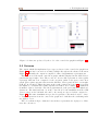
5.4 Outcome . . . . . . . . . . . . . . . . . . . . . . . . . . . . . . . . .
.
.
.
.
.
.
.
.
.
.
.
.
.
.
.
.
.
.
.
.
.
.
.
.
.
.
.
.
41
41
41
43
43
46
52
56
6 Evaluation
57
6.1 Correctness . . . . . . . . . . . . . . . . . . . . . . . . . . . . . . . . . . . 57
6.2 Usefulness . . . . . . . . . . . . . . . . . . . . . . . . . . . . . . . . . . . . 62
7 Conclusion and Future Work
63
v
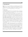
1 Introduction
Abstract The use of control flow graphs can be highly impractical in the quest for
gaining a deeper understanding of large program functions. An alternative control flow
visualization is proposed in this work, which projects the information about the control
flow within a function into a single scrolling dimension by abstracting it into structures
like choice, loop or optional execution with the help of regular expressions.
1.1 Motivation
Control flow graphs (CFG) constitute a program visualization technique commonly used
when analyzing the possible flow of control between the basic blocks of a program during
its execution. As such, many software analysis tools offer a feature for the automatic
generation of control flow graphs for given program code.
For large program functions, however, the resulting control flow graphs do become
rather huge, sometimes to the extent that they do not fit on the computer screen. If the
viewer’s objective is to examine a certain execution path for instance, he needs to scroll
left or right, up or down to display the portion of the control flow graph of interest. This
makes it difficult to keep track of the flow of control, especially while reading the code
details. Thus, control flow graphs can be impractical to use when trying to grasp the
inner workings of such large functions.
In an attempt to improve program comprehension, an alternative control flow visualization is presented in this work, we call it control flow blocks (CFB). The basic idea
is to use the property of containment instead of linkage to visualize the flow of control
between the basic blocks of a program: The visualization is basically a folded control
flow graph, in which all possible sequences of basic blocks composing an execution path
are mapped to one dimension. Meanwhile, the control flow is abstracted to explicit control flow structures like choice, loop and optional execution, which are represented by
box-like constructs enclosing the basic blocks that they apply to in the resulting overlay
of execution paths.
Regular expressions (RE) provide the basis for this control flow visualization. Describing the set of all possible execution paths within a control flow graph by means of a
regular expression over its basic blocks yields a one-dimensional representation. As for
the information about the control flow between the basic blocks, it is embodied in the
regular expression operators for concatenation, alternation and quantification. These
operators correspond to the box-like constructs, which they are mapped to once the
regular expression is derived in order to create the control flow visualization.
The resulting visualization makes it possible for the viewer to display and examine
an execution path of interest and hide all other information deemed irrelevant at the
moment. Moreover, fitting the height of the visualization to the screen space limits the
scrolling necessary to see other portions of a currently displayed execution path to one
direction only, making it as a whole far more readable than a control flow graph.
1
1 Introduction
A big concern in the generation of the control flow visualization are strongly connected
components in control flow graphs, because they entail regular expressions, which remain
non-minimal despite having been simplified as much as possible. In such regular expressions basic blocks occur multiple times. This causes basic block duplication to occur in
the control flow visualization as well, which has a negative effect on its compactness.
The weakening of a regular expression, which constitutes a further contribution, allows
sub-expressions to be replaced by expressions that are not as accurate but lead to a more
minimized overall regular expression.
The ultimate goal of this bachelor thesis is the implementation of a prototype that
produces the envisioned control flow visualization as output given a control flow graph
as input for the purpose of testing and evaluating the presented ideas.
1.2 Outline
This work is structured as follows: Chapter 2 elucidates in detail the reason why using
the visual property of containment instead of linkage to represent the control flow in
functions might be better. In Chapter 3, the theoretical foundations for computationally
deriving a regular expression for all possible execution paths in the control flow graph
are laid. The actual contributions of the work, which include the concept of control flow
blocks and the weakening of regular expressions, are introduced in Chapter 4. Chapter 5
presents details concerning the prototype of the envisioned program visualization tool
that was implemented for the purpose of testing the idea of control flow blocks, the
results are then discussed in Chapter 6. Finally, Chapter 7 provides a summary of this
work together with open questions that offer room for future investigation.
2
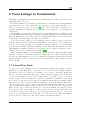
2 From Linkage to Containment
This chapter explains the foundations, based on which the idea for the control flow blocks
visualization was conceived.
Diehl has identified four visual properties that are commonly used in diagrammatic
representations to encode information about some aspect of a program, namely position,
linkage, neighbourhood and containment [1]. The control flow graph, for instance, is a
program visualization technique that uses linkage for the purpose of representing the
control flow.
The inspiration for using the visual property of containment instead of linkage comes
from LabVIEW, which is a dataflow visual programming language and environment from
National Instruments. It is widely used by scientists and engineers in the design and
development of measurement, test and control systems.
Visual programming (VP) goes in a different direction than program visualization
(PV) in what it achieves: In program visualization, some aspect of a program, here
it is the control flow, is mapped to a visual representation with the goal of enhancing
program understanding. Visual programming, on the other hand, is primarily concerned
with mapping a visual specification of a program to an executable program in order to
facilitate the process of software development [1, 2].
Still, generally speaking, both are mappings between program components and a visual
language. What is of particular interest here with respect to what is pursued in this
work are the visual languages or, more specifically, the graphical constructs in the visual
languages that are used to convey the control flow information. These will be reviewed
in the following.
2.1 Control Flow Graph
A control flow graph (CFG) is a directed graph that visualizes all possible execution
paths in a program. Each node corresponds to one of the basic blocks (BB), which the
program is composed of. These are groupings of one or more consecutive instructions
that are executed sequentially. The edges of the control flow graph represent the flow
of control between these basic blocks. It is important to note that once the control flow
reaches a basic block, it remains there until every instruction within the basic block
is executed. It only leaves upon completion, with the last instruction causing a jump.
Since a basic block is executed as a unit, branching in or out in the middle is impossible.
In the control flow graph, a basic block may have multiple incoming and outgoing
edges, meaning that it has as many possible predecessors and successors respectively.
There are two types of basic blocks that pose exceptions, namely the entry blocks and
the exit blocks. The entry blocks do not have any predecessors, whereas the exit blocks
do not have any successors. Therefore, all control flow enters through one of the entry
blocks to a program and leaves it through one of the exit blocks. Although multiple
entry blocks are possible in a control flow graph, it is rather uncommon.
3
2 From Linkage to Containment
Because the information about the flow of control within a program is visualized by
linkage, the explicitness and abstractness of the control flow structures, as known from
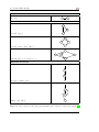
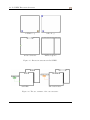
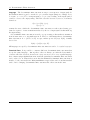
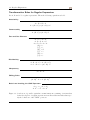
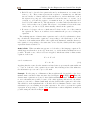
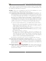
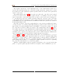
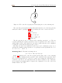
textual programming languages, do not really exist in a control flow graph. Nevertheless, certain patterns in the control flow graph can be associated to the basic control
flow structures and thus, at least, provide the information implicitly. Figure 2.2 is a juxtaposition of the basic textual high-level control flow statements and the corresponding
control flow graph patterns. In this figure, the B’s denote the relevant basic blocks, C
stands for a basic block that evaluates a boolean jump condition and V indicates a basic
block where a variable is evaluated before jumps are performed.
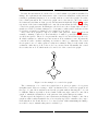
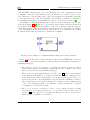
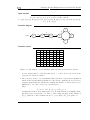
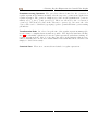
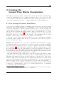
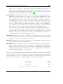
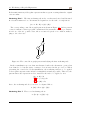
Any control flow graph is composed of these basic patterns. Figure 2.1 shows an
example consisting of six nodes. It is basically a do-while loop and an if-else construct
executed in sequence. The node A represents the entry block. It is followed by the node
B, which evaluates a condition upon its execution. If it evaluates to true, B passes the
control flow back to A, thus completing one iteration of the loop. Otherwise, the control
flow is passed on to C, where again a condition is evaluated. Based on the result of the
evaluation, either the node D or the node C are executed next. Eventually, the control
flow reaches the node F , which is the sole exit block of the control flow graph.
A
B
C
D
E
F
Figure 2.1: An example of a control flow graph.
The construction of a control flow graph based on given program code is pretty
straightforward. However, trying to draw conclusions from a control flow graph about
the type of control flow structures used in the program without knowing the code can
be difficult. This is especially so if faced with a rather strongly connected control flow
graph, fo which the identification of the patterns often yields ambiguous results.
In this regard, the high-level control structures underlying the example control flow
graph are rather easily identifiable due to how it is layouted. If, for instance, the component with the nodes A and B were to be rotated by 180◦ while maintaining the linkage,
it would be easy to mistake that part for a while-loop.
4
2.1 Control Flow Graph
Sequential Execution Structure
B1
B1 ; B1 ;
B2
Selection Structures
C
T
B1
F
if (C) {B1 ;}
C
F
T
B2
B1
if (C) {B1 ;} else {B1 ;}
V
B1
...
B2
Bn
switch (V ) { \* cases *\ }
Repetition Structures
B1
T
C
F
do {B1 ;} while (C);
C
T
F
B1
while (C) {B1 ;}
Figure 2.2: An overview of the basic patterns that can occur in a control flow graph. [3]
5
2 From Linkage to Containment
2.2 LabVIEW Execution Structures
In what follows, the concepts of virtual instruments and block diagrams in LabVIEW
[4, 5] will be introduced first, before turning to the execution structures, which are the
visual constructs used to represent the control flow in LabVIEW programs.
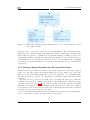
Virtual Instruments Programs created with LabVIEW are called virtual instruments
(VI). A virtual instrument consists of three components: The front panel is the user
interface containing controls for entering the inputs to the virtual instrument and indicators for presenting the outputs of the computation. The computation to be performed
by the virtual instrument is specified in the block diagram in terms of constructs of the
visual data flow programming language G. The icon and connector pane defines how the
inputs and outputs are wired to the icon representing the virtual instrument so that it
can be re-used in other virtual instruments.
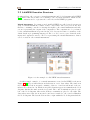
Figure 2.3: An example of a LabVIEW virtual instrument.
A rather simple example of a virtual instrument created in LabVIEW is shown in
Figure 2.3 [5]. It performs addition and subtraction on two data values. The window in
the background is the front panel consisting of the two controls a and b and of the two
indicators a + b and a − b. All the front panel elements appear as terminals in the block
diagram, which is the window in the foreground. The control terminals are placed to the
left of the block diagram, whereas the indicator terminals are placed to the right. The
data values entered into the front panel controls are forwarded to the control terminals in
the block diagram. The data flows from left to right within the block diagram while the
6
2.2 LabVIEW Execution Structures
functions are performed and new data values are produced. These flow to the indicator
terminals and are displayed in the front panel indicators eventually.
Block Diagram
The block diagram is a directed acyclic graph composed of:
• Terminals: The terminals serve as sources or sinks for data in the block diagram.
The color of a terminal provides information on the type of data it handles.
There are those terminals that interact with the front panel objects. The terminals
corresponding to the controls on the front panel are called control terminals, while
those corresponding to the indicators on the front panel are called indicator terminals respectively. The control terminals propagate the input data received from
the controls to the block diagram, the indicator terminals update the indicators
on the front panel with the output data.
But there are also terminals, which do not correspond to any element on the front
panel. Therefore, the data values that they supply the block diagram with cannot
be modified by the user during the execution of the virtual instrument. Such
terminals are referred to as constants.
• Nodes: Nodes are the places in the block diagram, where computation takes place.
They can be, for instance, built-in functions or icons of other virtual instruments.
All data values required as inputs by a node need to be available for it to execute.
Once this is the case, the node consumes the input data, performs the specified
computation on that data to finally produce outputs. The execution of the block
diagram as a whole is said to be data-driven, because the data flow through the
nodes determines when the nodes of the block diagram are executed.
• Wires: Wires are the edges in the acyclic graph and determine the paths, along
which data propagates through the block diagram. Each wire connects one source
with at least one target. In case of a fan-out to many targets, the data value is
duplicated to be send to each target. The color, style and thickness of the wires
depend on the type of data that pass through them.
Execution Structures Until now, no components that could be used to manipulate the
execution order of the nodes within a block diagram were mentioned. However, control
flow structures that enforce sequential, conditional or iterative execution on parts of
the block diagram, where otherwise the execution order of the nodes depends on the
availability of the input data, would make the visual dataflow programming language a
lot more expressive.
If the language is to include control flow structures, these must be represented by
entirely new visual constructs: The block diagram is a directed acyclic graph, where
the nodes and edges, which are about all the components that any graph consists of,
already have meanings assigned to them. Where in control flow graphs linkage is used to
illustrate the flow of control, the same property is used in the block diagrams to encode
information about the data flow.
7
2 From Linkage to Containment
In LabVIEW, this issue has been solved with the use of the containment property
to visualize control flow. The language has been extended by so-called execution structures, which are boxes enclosing parts of the block diagram and essentially behave like
nodes towards the rest of the block diagram. The resulting combination of structured
programming and dataflow programming is referred to as structured dataflow [6].
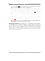
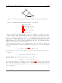
An example of a virtual instrument, where such an execution structure comes to use,
is shown in Figure 2.4 [5]. The for loop structure takes a value 0 and increments it in
five iterations. The elements at the junction of the for loop structure with the wires are
called shift registers. They make sure that data from the previous iteration is available
to the computation in the next iteration. When the for-loop terminates, the 5-times
incremented data value is forwarded to an indicator terminal.
Figure 2.4: An example of a virtual instrument using an execution structure.
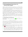
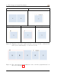
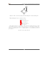
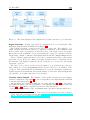
Figure 2.5 shows all of the execution structures offered by LabVIEW that correspond
semantically to control flow structures commonly known from high-level textual programming languages:
• The while loop structure executes its code at least once and stops when a condition
is met. With regard to its semantics, it rather matches the do-while or the repeatuntil loop in text-based programming languages.
There are two special terminals inside of it: The count i in the bottom left-hand
corner indicates the number of completed iterations. It starts counting at zero
in the first iteration and is incremented for each subsequent iteration. The continuation flag in the bottom right-hand corner specifies the termination behavior.
After each iteration, it is checked whether the condition for the termination has
ocurred. Per default, the while loop terminates on true, but this can be changed
to termination on false if necessary.
• The for loop structure executes its code zero or more times, but there is a limit
specified as to how many iterations are to be performed at most. The iteration
terminal N in the upper left corner inside the structure is wired to a data source,
which sets the total number of iterations.
8
2.2 LabVIEW Execution Structures
1 While loop
2 For Loop
3 Case Structure
4 Flat Sequence
Figure 2.5: Execution structures in LabVIEW.
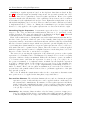
3.1 If-Else
3.2 Switch-Cases
Figure 2.6: The two variants of the case structure.
9
2 From Linkage to Containment
The count terminal i in the bottom left corner of the structure that contains the
number of performed iterations. It start counting at zero.
• The case structure contains two or more subdiagrams, each of which constitutes
a case. Only one case can be viewed at a time; the case selector label at the top
of the structure allows to switch between the different subdiagrams. Among all
cases, only one is executed. The structure has a selector terminal ? on its border,
which determines the case to execute depending on its input.
The data source wired to the selector terminal must be either an integer, a Boolean
value, a string or an enumerated type. A case structure with a Boolean selector
corresponds to an if-else statement as known from textual programming languages,
while a case structure with a selector of any other allowed data type corresponds
to a switch-cases construct. The two variants of this execution structure are shown
in Figure 2.6.
• The flat sequence structure forces sequential execution upon its subdiagrams. The
subdiagrams are executed in order from left to right.
Advantages of Containment The visual property of containment, as taken advantage
of in LabVIEW, provides a means for reducing the cognitive burden on the viewer: It
allows to abstract the control flow into explicit execution structures. These structures
make it possible to specify computations, which would result in huge block diagrams
otherwise, in a concise manner. This is especially so for the case execution structure,
which shows only one case at a time; all other information that are deemed not relevant
for the moment are simply hidden.
10
3 Deriving Regular Expressions for
Control Flow Graphs
Deriving a regular expression that represents the control flow of a program by hand is
fairly easy when given a control flow graph of manageable size. For any control flow graph
that goes beyond that, it makes sense to have a computational method that does the job.
In fact, with the intention of implementing a prototype of the envisioned visualization
tool, finding such a method is compulsory.
For our purposes, the equivalence of deterministic finite automata and regular expressions within the Chomsky hierarchy as known from formal language theory turns out to
be usable. Deterministic finite automata prove themselves to be quite similar to control
flow graphs upon closer inspection. Hence, they can serve as means of formalization,
such that the problem of transforming a control flow graph into a regular expression is
reduced to the problem of converting a deterministic finite automaton to an equivalent
regular expression, for which textbook solutions exist.
With this chapter the theoretical foundations for the remainder of this work will be
laid. The deterministic finite automaton model and the algebra of regular expressions
will be introduced, after which methods for the conversion between both representations
will be reviewed.
3.1 Determininstic Finite Automata
Formal Definition
by the five-tuple
A deterministic finite automaton [7, 8] (DFA) A is formally denoted
A = (S, Σ, δ : S × Σ → S, s0 , F ),
where S is a finite set of states, Σ is a finite input alphabet, δ is the transition function
that determines the next state given a state and an input symbol, s0 ∈ S is the start
state and F ⊆ S is the set of final states. It is deterministic because in any of its states
and for any input symbol that is accepted at that particular state, there is only one
possible next state it can transition to.
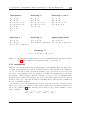
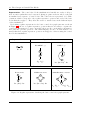
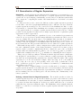
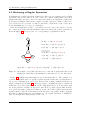
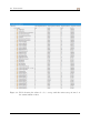
Representations Apart from the five-tuple that is the formal notation for a deterministic finite automaton, there are two other possible representations, which are shown in
Figure 3.1. These will be introduced in the following:
• The transition diagram is the graph representation of the deterministic finite automaton. The nodes represent the states. The one node corresponding to the start
state is marked with an incoming edge originating from nowhere. All nodes are
drawn as circles, except for the ones that correspond to the final states, in which
case the nodes are designated by double circles. Meanwhile, the directed edges
represent the transitions between the states. If for any two states i, j ∈ S there
11
3 Deriving Regular Expressions for Control Flow Graphs
Tuple notation
A = (S = {q0 , q1 , q2 , q3 , q4 , q5 , q6 }, Σ = {a, b, c, d, e, f },
δ = {(q0 , a, q1 ), (q1 , b, q2 ), (q2 , a, q1 ), (q2 , c, q3 ), (q3 , d, q4 ), (q3 , e, q5 ), (q4 , f , q6 ), (q5 , f , q6 )},
s0 = q0 , F = {q6 })
Transition diagram
q5
a
start
q0
a
q1
b
f
e
q2
c
q3
q6
d
q4
f
Transition matrix
T
q0
q1
q2
q3
q4
q5
q6
q0
∅
∅
∅
∅
∅
∅
∅
q1
a
∅
a
∅
∅
∅
∅
q2
∅
b
∅
∅
∅
∅
∅
q3
∅
∅
c
∅
∅
∅
∅
q4
∅
∅
∅
d
∅
∅
∅
q5
∅
∅
∅
e
∅
∅
∅
q6
∅
∅
∅
∅
f
f
∅
Figure 3.1: An example of a deterministic finite automaton in various notations.
is some input symbol a ∈ Σ such that δ(i, a) = j, there is an edge between the
respective nodes labeled with a.
• The transition matrix of a deterministic finite automaton represents its transition
function and is particularly well-suited for the use in computations. Let T denote
a square matrix with the dimensions equaling the number of states in the set S.
Furthermore, let i and j denote two specific states.
Then
∀i, j ∈ S, a ∈ Σ : δ(i, a) = j ⇒ T [i, j] = a,
meaning that if there is an input symbol a ∈ Σ, such that the deterministic finite
automaton moves from state i to state j, there exists an entry in the matrix at
T [i, j], which is a. If no transition from i to j is possible, T [i, j] is equal to ∅.
12
3.1 Determininstic Finite Automata
Language The deterministic finite automaton can process sequences of input symbols.
Its transition function can be extended to process these input strings accordingly. Let s
be a state, ω = υa ∈ Σ∗ be an input string to be processed ending on the input symbol
a and let denote the empty string. Then the extended transition function, recursively
defined as
δ̂(s, ω) = δ(δ̂(s, υ), a),
δ(s, ) = s,
returns the state, which the deterministic finite automaton reaches after having performed a sequence of state transitions induced by the set of input symbols that make up
the input string.
A deterministic finite automaton is said to accept a string ω that makes it transition
from its start state s0 to any final state in F . The set of all strings that a deterministic
finite automaton A = (S, Σ, δ, s0 , F ) accepts, makes up its language L(A), formally
denoted as
L(A) = {ω|δ̂(s0 , ω) ∈ F }.
All languages accepted by deterministic finite automata are said to be regular languages.
Canonical Form It is possible to construct different deterministic finite automata that
accept the same language. Among these, there is always one with the least number
of states called the minimal deterministic finite automaton. For every regular language
there exists a unique minimal automaton and all equivalent deterministic finite automata
can be reduced to it. That is the reason why the minimal deterministic finite automaton
is said to be the canonical form. Many minimization approaches can be found in standard
textbooks for bringing deterministic finite automata into their canonical forms.
13
3 Deriving Regular Expressions for Control Flow Graphs
3.2 Regular Expressions
In formal language theory, regular expressions [7, 8] are used to describe regular languages in a concise manner. For the purpose that is pursued here, a closer look at the
algebra of regular expressions and the underlying axioms is necessary, where especially
the effects of the regular expression operators on the languages these expressions represent need to be examined thoroughly. In the following, the notation L(E) will be used
to denote the language accepted by a regular expression E.
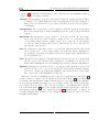
Basic Regular Expressions
The following constants are defined as regular expressions:
• A regular language is defined over a finite alphabet Σ. For all symbols a ∈ Σ, a
regular expression a, where L(a) = a, needs to be introduced.
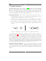
• The empty set ∅ is a regular expression that denotes the language ∅, that is L(∅) =
∅. In the algebra of regular expressions, this constant represents the zero element.
• The empty string is a regular expression that denotes the language {}, that is
L() = {}. In the algebra of regular expressions, this constant represents the one
element.
start
s
f
start
s
f
Figure 3.2: The difference between the empty set ∅ and the empty string .
On the first glance, ∅ and might look the same, but there is indeed a difference, as
illustrated in Figure 3.2. The deterministic finite automaton on the left corresponds to
the language denoted by ∅. No input string could take this automaton from its start
state to its final state. Hence, the language that it accepts, equals the empty set. With
the deterministic finite automaton on the right, on the other hand, it is possible to
transition from the start state to the final state: As soon as the automaton is in in its
start state, it will automatically transition to its final state. In fact, the automaton can
be reduced to a single state, where the state is both the start and the final state. That
is why the language that this automaton accepts is made up of only.
Basic Regular Expression Operators More complex regular expressions can be built
inductively over the previously defined constants by means of the following three essential
operators. The semantics of the operators that can be applied to regular expressions, are
presented with respect to how they affect the sets of strings that these regular expressions
stand for.
14
3.2 Regular Expressions
Let M and N be two regular expressions. Then:
Alternation: M +N is a regular expression that denotes the set union or sum of the
languages L(M ) and L(N ), such that L(M +N ) = L(M ) ∪ L(N ). If m is the
number of strings in L(M ) and n is the number of strings in L(N ), then L(M +N )
contains m + n strings as a result of this operation. In the literature, the symbols
+ and | are used interchangeably.
Concatenation: M ·N is a regular expression that denotes the concatenation or product of the languages L(M ) and L(N ), such that L(M ·N ) = L(M ) · L(N ). The
concatenation of the languages L(M ) and L(N ) yields the set of strings that can
be formed by taking any string in L and concatenating it with any string in M .
Therefore, if m is the number of strings in L(M ) and n is the number of strings
in L(N ), then L(M ·N ) contains m · n strings. Note that the dot operator can be
omitted.
Star: M ∗ is a regular expression, which is an abbreviating notation for +M +M M +. . . .
It denotes the closure or iterate of L(M ), such that L(M ∗ ) = (L(M ))∗ , which is
the set of strings that can be constructed by concatenating L(M ) with itself any
number of times. This can be denoted more formally as
S
i
(L(M ))∗ = ∞
i≥0 L(M ) ,
where
(L(M ))i = L(M ) · (L(M ))i−1 ,
(L(M ))1 = L(M ) and (L(M ))0 = {}.
Any regular expression can be constructed using these operators in finitely many steps.
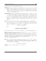
Additional Regular Expression Operators Although the operators for concatenation,
alternation and star are sufficent to construct any regular expression and, hence, to
express any regular language, the following two operators, that might be known from
the UNIX environment, are quantification operators added as syntactic sugar. They
allow it to express a regular expression in a more concise manner.
Let M be a regular expression.
Plus: M + is a regular expression, which is a short hand for M · M ∗ or M ∗ · M , and is
called the positive closure. It is basically the same as the closure defined above,
except that L(M + ) = (L(M ))+ does not contain the empty string . The operation
can be denoted more formally as
S
i
(L(M ))+ = ∞
i≥1 L(M ) .
Optional: M ? can be written instead of + M or M + .
15
3 Deriving Regular Expressions for Control Flow Graphs
Precedence among Operators The precedence that is defined for the operators of
regular expressions determines, in which order the respective operations are applied in a
regular expression. The operators of highest precedence are the quantification operators,
namely star (∗ ), plus (+ ) and optional (?). These are followed by the concatenation
operator (·). Of lowest precedence is the alternation operator (+). Of course, the order
of precedence can be overridden by grouping together operands and their operators using
parentheses.
Transformation Rules In order to keep the size of the regular expressions manageable,
it is necessary to simplify them as much as possible. The algebraic laws listed in Figure 3.3 are essentially equivalences between regular expressions, such that rewriting one
regular expression as the other, does not have any effect on the language that is represented. Actually, there are far more transformation rules than listed here, but these can
simply be derived if necessary.
Canonical Form There is no canonical form defined for regular expressions.
16
3.2 Regular Expressions
Transformation Rules for Regular Expressions
Let A, B and C be regular expressions. Then the following equivalences hold:
Associativity
A+B =B+A
A + (B + C) = (A + B) + C
Commutativity
A · (B · C) = (A · B) · C
Zero and One Elements
A·=·A=A
A·∅=∅·A=∅
A+∅=∅+A=A
(∅)∗ = ()∗ = (∅)+ = ∅
()+ = (∅)? = ()? = Distributivity
A · B + A · C = A · (B + C)
A · C + B · C = (A + B) · C
Idempotency
A+A=A
Shifting Rules
(A · B)∗ · A = A · (B · A)∗
Basic Laws Involving the UNIX Operators
A + = + A = A?
A · A∗ = A∗ · A = A+
Figure 3.3: A selection of possible equivalence transformations consisting of axioms that
define the algebra of regular expressions as well as additional rules that specify the behaviour of the UNIX operators.
17
3 Deriving Regular Expressions for Control Flow Graphs
3.3 Converting a Deterministic Finite Automaton
to a Regular Expression
There are many methods to compute a regular expression that describes the language
of a deterministic finite automaton, of which two will be reviewed in the following.
3.3.1 Transitive Closure Method
The transitive closure method [7, 8] is an inductive approach to constructing a regular
expression for a deterministic finite automaton. Starting off from paths that do not pass
through any of the states in the deterministic finite automaton, regular expressions are
built for an increasingly growing set of paths as the number of states, through which
they are allowed to go, grows gradually. Upon reaching the total number of states, the
regular expression that describes all possible sequences of transitions in the deterministic
finite automaton is obtained.
Without loss of generality, let the deterministic finite automaton be denoted by A =
(S, Σ, δ, s0 , F ) and let S be a finite set of n states, each of which is uniquely identifiable
by a number between 1 and n. Moreover, let the set of paths from state i to state
j, where no intermediate state is numbered greater than k, be denoted by the regular
(k)
expression Ri,j .
(k)
The construction of the regular expressions Ri,j for all i, j ∈ S and for all k, for which
0 ≤ k ≤ n hold, can be defined inductively as follows:
(0)
k = 0:
The regular expressions Ri,j basically denote all the paths between any two
states i and j having no intermediate states. They are defined as follows:
(
r
if i 6= j
(0)
Ri,j =
r + if i = j
r is a regular expression obtained by applying the alternation operator to the labels of
all edges between two states i and j. If no transition between i and j exists, then r is
set to ∅.
(k)
k ≤ n:
The regular expressions Ri,j represents the paths between the states i and j
that do not pass through any state with a higher number than k. It can be constructed
in terms of the regular expressions obtained during the previous induction step k − 1
like so:
(k)
(k−1)
Ri,j = Ri,j
(k−1)
+ Ri,k
(k−1) ∗
· (Rk,k
(k−1)
) · Rk,j
.
(3.1)
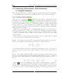
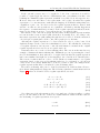
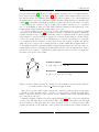
Figure 3.4 provides an explanation for this equation. Basically, the set of paths de(k)
(k−1)
scribed by the regular expression Ri,j is the union of the set of paths Ri,j
that do not
have the state k as intermediate state and of the set of paths that do. Paths belonging
to the latter set have a common structure in that there is a part going from state i to
18
3.3 Converting a Deterministic Finite Automaton to a Regular Expression
(k−1)
Ri,j
j
i
(k−1)
(k−1)
Ri,k
Rk,j
k
(k−1)
Ri,k
j
i
(k−1)
Ri,j
(k−1)
+ Ri,k
(k−1) ∗
)
· (Rk,k
(k−1)
· Rk,j
Figure 3.4: Illustration of the effects of the k-th induction step on a deterministic finite
automaton as specified by the equation in (3.1).
state k, another part that possibly denotes the repetetive traversal of the self-loop at
state k, and yet another part going from state k to state j. Therefore, paths of this type
(k−1)
(k−1)
(k−1)
can be represented by the regular expression Ri,k · (Rk,k )∗ · Rk,j .
After having performed all n induction steps, the regular expression that represents
the behaviour of the whole deterministic finite automaton is the union of all regular
(n)
expressions Ri,j , where i is the number of the start state s0 and j corresponds to one
of the final states F .
3.3.2 Brzozowski’s Method
Brzozowski presents an algebraic method [9, 10, 11] for converting a deterministic finite
automaton into a regular expression: A system of linear equations, so-called characteristic equations, is created, which describes the behavior of the automaton. By solving
this system of equations, the regular expression that is equivalent to the deterministic
finite automaton in the language it accepts, can be obtained.
Let the deterministic finite automaton be denoted by M = (S, Σ, δ, s0 , F ). Furthermore, let S be a finite set of n states, where each state is uniquely identifiable by a
number i between 1 and n. For each state i ∈ S a characteristic equation is constructed
like so:
1. Each state i ∈ S is associated with an unknown Xi . This unknown represents the
set of input strings that make M move from that state to one of its final states in
F.
19
3 Deriving Regular Expressions for Control Flow Graphs
2. Each Xi can be described in equational form by an alternation over terms of the
form ai,j · Xj . These terms represent the sequences of transitions over different
successor states of i that it takes for the automaton to reach a final state; each of
the sequences is composed of the transition between the state i to a state j ∈ S
on input ai,j ∈ Σ and the sequence of transitions from j to any final state in F
denoted by the unknown Xj . The alternation over these indicates that there is a
choice between these sets of paths. The absence of a transition between the state
i and a state j is denoted by ∅, this is usually omitted in the equations.
3. If a state i belongs to the set of final states F , then is also one of the terms in
the equation Xi . Later on, it will act as a terminal in the process of solving the
equations.
The resulting system of characteristic equations can be solved by substitution. Starting off with the characteristic equations corresponding to the final states of M , the
occurrences of the unknowns in all the other equations is eliminated, until the characteristic equation corresponding to the start state s0 is solely left, which yields the regular
expression that is searched for.
Arden’s Rule When an unknown appears on both sides of the language equation Xi ,
which happens when there is an edge from state i to itself, further substitution is not
possible. In such a case, Arden’s theorem is applied, which states that a characteristic
equation of the form
X =A·X +B
can be rewritten as
X = A∗ · B.
(3.2)
Applying this theorem solves the situation at hand, since it prevents the same unknown
to occur on both side of the equation as a result. After having isolated the unknown,
the substitution process can be proceeded with.
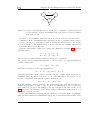
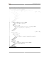
Example For the purpose of illustration, Brzozowski’s method is applied to the deterministic finite automaton that was introduced in Figure 3.1, in Figure 3.5. First, the
characteristic equations are derived, after which substitution starts. This is done until
no more substitution is possible because of X2 . After applying Arden’s rule, the substitution process can be continued with until only the characteristic equation for X0 is left.
The variables on the right-hand side of X0 have all been eliminated in the course of the
substitution process resulting in a regular expression. In order to prevent the regular
expression from growing too much, every intermediate result is simplified as much as
possible using the rules from Figure 4.4.
20
3.3 Converting a Deterministic Finite Automaton to a Regular Expression
X0
X1
X2
X3
X4
X5
X6
Eliminating X4 and X5 :
Eliminating X6 :
The Equations:
= a · X1
= b · X2
= a · X1 + c · X3
= d · X4 + e · X5
= f · X6
= f · X6
=
X0
X1
X2
X3
X4
= a · X1
= b · X2
= a · X1 + c · X3
= d · X4 + e · X5
= X5 = f
X0
X1
X2
X3
= a · X1
= b · X2
= a · X1 + c · X3
=d·f +e·f
Eliminating X3 :
Eliminating X1 :
Applying Arden’s Rule:
X0 = a · X1
X1 = b · X2
X2 = a · X1 + c · (d + e) · f
X0 = a · b · X2
X2 = a·b·X2 +c·(d+e)·f
X0 = a · b · X2
X2 = (a · b)∗ · c · (d + e) · f
Eliminating X2 :
X0 = a · b · (a · b)∗ · c · (d + e) · f
Figure 3.5: Applying Brzozowski’s method to the deterministic finite automaton in Figure 3.1. The result is the expression (a · b)+ · c · (d + e) · f .
3.3.3 Juxtaposition
What the two presented methods for transforming a deterministic finite automaton into
a regular expression have in common, is that the states of the automaton are eliminated
one by one and the regular expressions labeling edges between the predecessors and
successors of an eliminated state are updated to include the missing state’s behaviour
progressively. This guarantees that the language accepted by the deterministic finite
automaton is the same as the language accepted by the final regular expression, which is
the label of the edge connecting the last two remaining states, when the state elimination
process eventually terminates.
As a matter of fact, the similarity in how these methods work can be sketched easily.
The key to doing so is to link the characteristic equations in combination with Arden’s
rule to the equation (3.1) that was introduced in the section on the transitive closure
method, namely
(k)
(k−1)
Ri,j = Ri,j
(k−1)
+ Ri,k
(k−1) ∗
)
· (Rk,k
(k−1)
· Rk,j
.
21
3 Deriving Regular Expressions for Control Flow Graphs
Ai,j
i
Ai,k
k
j
Ak,j
Ak,k
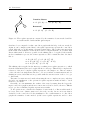
Figure 3.6: Setup for showing that the two methods for computing a regular expression
for the language a given deterministic finite automaton accepts are similar
in how they work.
Let there be a deterministic finite automaton and let the state k be the next state to
be eliminated. If the deterministic finite automaton is able to transition from a state i
to a state j, it can do so either with or without passing through the state k, and, in case
it does, it can also go through the self-loop at k repeatedly. Let’s assume, without loss
of generality, that both are the case.
Deriving characteristic equations for this setup, illustrated in Figure 3.6, is pretty
straightforward:
Xi = Ai,j · Xj + Ai,k · Xk
Xk = Ak,j · Xj + Ak,k · Xk ,
The A’s denote regular expressions that are the labels of transitions.
The equation Xk necessitates the application of Arden’s rule before any substitution is
possible, which yields:
Xk = (Ak,k )∗ · (Ak,j · Xj )
Then, the following is obtained per substitution:
Xi = Ai,j · Xj + Ai,k · (Ak,k )∗ · Ak,j · Xj
Currently, this characteristic equation describes the set of paths, which brings the deterministic finite automaton from state i to one of the final states. Let’s ignore Xj for
the sake of argument, such that the equation is shortened to:
Xi,j = Ai,j + Ai,k · (Ak,k )∗ · Ak,j
Now, the language equation stands for the input strings that cause the automaton to
transition from state i to state j only. Upon closer examination it can be found that
this equation is, except for the naming of the sub-expressions, the same as the one in
(3.1). In essence, the transitive closure method achieves what Brzozowski’s method does
in multiple steps, in one step.
Despite this similarity, applying the two methods to the same input deterministic
finite automaton without any simplification performed on the intermediate results, yields
22
3.3 Converting a Deterministic Finite Automaton to a Regular Expression
regular expressions that describe the same regular language, but actually look different:
The transitive closure method tends to produce rather long regular expressions compared
to Brzozowski’s method [11].
This is due to the difference in the order, in which both methods eliminate the states
in the deterministic finite automaton. The choice concerning the order of state removal
affects the size of the regular expression that results from the computation.
With the transitive closure method, there are no inherent restrictions as to how the
state removal sequence is chosen, it always works. For an automaton consisting of n
states there are n! possible sequences and equally as many diffferent possible results. By
contrast, Brzozowski’s method starts from the automaton’s final states and eliminates in
each step the immediate predecessors of the states that were eliminated in the previous
step. Consequently, the state removal sequence is pretty much determined; the created
result is a relatively compact regular expression.
23
4 Creating the
Control Flow Blocks Visualization
This chapter presents the main contributions of this work: The first is an alternative
control flow visualization based on regular expressions, called control flow blocks. The
second comprises of the efforts to minimize the regular expressions by means of normalization and weakening for the sake of compact control flow blocks visualizations.
4.1 The Concept of Control Flow Blocks
Control flow blocks (CFB) constitutes a visualization method for the control flow between
a program’s basic blocks, intended to be an alternative to the control flow graph. This
control flow visualization contains as much information as a control flow graph, but
presents this information on a computer screen in a way that necessitates scrolling in
only one direction, either horizontally from left to right or vertically from top to bottom
depending on personal preference.1 Moreover, it allows the viewer to temporarily hide
information that is not of interest for the moment. The visualization is not geared
towards a certain audience; it is meant to be intuitive to understand.
The basic concept behind control flow blocks, the process of generating the visualization and the visual constructs that are used to represent the control flow are described
in more detail in what follows.
Concept The visualization is to recover the explicitness and abstractness of control
flow structures that are non-existent in a control flow graph by following LabVIEW’s
approach of using the visual property of containment. The problem is that the mapping
shown in Figure 2.2 only works well in one direction. Trying to simply map the control
flow graph patterns back to the basic high-level control flow structures, for instance, is
not as straightforward. Especially with control flow graphs that are more complex in
their structure, it is hard to unambiguously associate patterns in the graph with concrete
control flow structures without knowing the code details.
But what is known for sure, when given a control flow graph, is the number of times
each of the basic blocks along an execution path are executed during a program run.
That kind of information about the execution paths can be expressed in a concise way by
means of regular expressions. What the use of regular expressions provokes is the folding
of the control flow graph, such that all execution paths are projected onto one dimension,
while the regular expression operators abstract the control flow into structures like loop,
choice or optional execution. These structures in the regular expression can then simply
be mapped to a visual language composed of constructs that make use of containment
to convey the control flow information.
1
The general orientation of the control flow blocks visualizations that will be shown for presentation
purposes in the remainder of this work is set to be horizontal.
25
4 Creating the Control Flow Blocks Visualization
The concept of control flow blocks is agnostic about the program code specifics. Thus,
it can be applied regardless of the level of abstraction in the programming language that
the examined program function is written in.
Workflow The process of generating the control flow blocks visualization for a given
control flow graph can be roughly divided into three steps:
From Control Flow Graph to Deterministic Finite Automaton: The equivalence of deterministic finite automata and regular expressions is usable in reducing the problem of transforming a control flow graph into a regular expression to the problem
of converting a deterministic finite automaton to an equivalent regular expression.
There is no need for much modification when turning a control flow graph into a
deterministic finite automaton, since they are already very similar. The property
of determinism is also present in the control flow graph, in that it is not possible
to jump to and execute two different basic blocks at the same time. Also, it is not
possible for the same block to be addressed by two different jump addresses.
A control flow graph is transformed into a deterministic finite automaton like so:
• All nodes of the control flow graphs are reinterpreted as states of a deterministic finite automaton. Each node of the control flow graph is assigned a
unique identifier i and is then added to the set S.
• A new state is introduced, which is linked to all states representing an entry
block. This state is designated as the start state s0 .
• All states corresponding to an exit block are declared as final states by adding
them to the set F .
• Σ contains the identifiers of all states.
• The edges of the control flow graph are reinterpreted as transitions of the
deterministic finite automaton. Each transition arc is labeled with the identifier of the target state. A label can be thought of as an address of the next
basic block that will be jumped to during program execution. The transition
function δ can be specified straightforwardly afterwards.
Following these steps always yields a minimal deterministic finite automaton.
From Deterministic Finite Automaton to Regular Expression: Once the deterministic
finite automaton is obtained, it is easy to compute a regular expression that accepts the same language. Two standard textbook solutions for accomplishing this
task, the transitive closure method and Brzozowski’s method, have already been
introduced in Section 3.3.
From Regular Expression to Control Flow Blocks: The regular expression that is the
output of the previous step is finally mapped to the control flow blocks visualization. The set of visual constructs that such a visualization is composed of will be
presented in the following.
26
4.1 The Concept of Control Flow Blocks
Representation The control flow blocks visualization is basically an overlay of all possible execution paths that can be traversed during program execution, where each path
is visualized as a sequence of basic blocks. The control flow is represented by box-like
constructs, which correspond to the regular expression operators and enclose the basic
blocks that they apply to. They allow the viewer to switch between the different layers
of the visualization.
By deriving regular expressions for the basic control flow graph patterns, as shown
in Figure 4.1, the set of regular expression operators that are necessary to capture the
control flow information becomes conceivable; these are the concatenation, alternation,
star, plus and optional operators. The visual language needs to at least include constructs that these regular expression operators are mapped to when creating the control
flow blocks visualization.
Sequence Structure
Repetition Structures
do-while loop
B1
while loop
B2
b1 · b2
B1
B1
B2
B2
B3
(b1 · b2 )+
b1 · (b2 · b1 )∗ · b3
Selection Structures
if -statement
if-else-statement
switch-cases construct
B1
B1
B1
T
F
B2
B3
B2
B2
B3
b1 · (b2 )? · b3
...
Bn
B4
b1 · (b2 + b3 ) · b4
Bn+1
b1 · (b2 + · · · + bn ) · bn+1
Figure 4.1: Regular expressions describing the basic control flow graph patterns.
27
4 Creating the Control Flow Blocks Visualization
Figure 4.2 presents the visual language of the control flow blocks visualization that is
composed of the following constructs:
Terminal: The terminals correspond to the basic blocks in the regular expression. They
are simple boxes, which display the basic block instructions. For the remainder of
this section, let a and b denote two basic blocks that are part of the program to
be visualized.
Concatenation: The concatenation operator applied to a and b, as in a · b, denotes that
b is executed right after a. In the visualization, the two basic blocks are shown in
sequence.
Alternation: The alternation operator applied to a and b, as in a + b, denotes the
choice between the two basic blocks as to which one is to be executed next. The
corresponding visual construct consists of tabs, one for each case. It only displays
one case at a time and allows the viewer to switch from one case to any other by
selecting the respective tab.
Star: The application of the star operator to a, as in (a)∗ , indicates that the basic block
can be executed zero or more times during a program run. In the visualization,
the terminal representing a is simply enclosed by a frame with a small indicator
for the quantifier type.
Plus: The plus operator applied to a implies that a is executed at least once. As it is with
the star operator, the expression (a)+ is mapped to a terminal for a enclosed by a
frame with a small indicator for the quantifier type when creating the visualization.
Optional: Applying the optional operator to a, as in (a)?, states that the basic block a
is either executed once or not at all. Again, the corresponding terminal is simply
enclosed by a frame representing this quantifier. The viewer is able to temporarily
hide components of the visualization of this type.
What the control flow visualization for the control flow graph introduced in Figure 2.1
would look like according to the aforementioned is shown in Figure 4.3. As a matter of
fact, many of the intermediate results obtained in the process of generating the visualization are already available and just need to be brought together: The result from the first
step, which is the conversion of the control flow graph to a deterministic finite automaton, is shown in Figure 3.1. As for the regular expression that captures the control flow
information, it has already been computed in Section 3.3, yielding (a · b)+ · c · (d + e) · f
as result. Mapping this expression to the visualization in the last step can be done in a
straightforward manner.
28
4.1 The Concept of Control Flow Blocks
a·b
(a)∗
a+b
(a)+
(a)?
Figure 4.2: Mapping between the regular expression operators and the constructs that
make up the visual language of control flow blocks.
Figure 4.3: The control flow blocks visualization for the control flow graph that has been
introduced in Figure 2.1.
29
4 Creating the Control Flow Blocks Visualization
4.2 Normalization of Regular Expressions
Motivation As already known, the different methods that have been presented for converting a given deterministic finite automaton to a regular expression yield results that
capture the accepted language semantically, yet they may look different syntactically.
As a consequence, comparing the results of the transformation to check their correctness
is difficult.
Looking at it in a broader context, the difference in the regular expressions generated
for the same control flow graph might ultimately lead to different outcomes, when the
regular expressions are mapped to the control flow blocks visualizations. But of course,
it is desirable to obtain the same visualization for an input control flow graph regardless
of the applied method for creating a regular expression that describes the set of all its
possible execution paths. For that reason, a unique representation for equivalent regular
expressions would be appreciated.
The process of transforming two equivalent objects to some standard representation is
referred to as canonicalization and the unique standard representation is called canonical
form accordingly. The canonical form of a deterministic finite automaton, for instance,
is the minimal deterministic finite automaton, and as shown in the previous section, converting a control flow graph to a deterministic finite automaton is proven to deliver one
in its canonical form. The problem is that there is none defined for regular expressions.
What makes it impossible to achieve uniqueness in regular expressions is the associative and commutative nature of the binary alternation operation: For a same-operator
sequence with n operands, commutativity allows to change the order
of the operands in
n
n! ways, while associativity makes it possible
to choose between 2 pairs of operands to
evaluate first, resulting in about n! · n2 possibilities for evaluating the whole sequence.
This poses a problem especially in combination with the algebraic laws for distributivity. If applied to an alternation of over more than two regular expressions, the distributive laws can yield semantically equivalent but otherwise different results. The regular
expression A + A · B + B is such an example, where factoring out A or B results in
A · ( + B) + B or A + (A + ) · B depending on the order of the operands and on how
these operands are grouped together for evaluation, determined by commutativity and
associativity respectively.
Thus, we resort to roughly defining a normal form that is fit for our purpose of using
regular expressions instead. A normal form can be seen as less than a canonical form in
that is does not guarantee uniqueness in the representations. Settling for a normal form
involves making some choices with regard to the associativity and commutativity of the
binary operations.
Defining a Normal Form for Regular Expressions The normal form that we define for
regular expressions needs to incorporate the desirable properties of the envisioned control
flow visualization: For the sake of compact visualizations, the regular expressions should
be minimal in that their lengths are as short as possible while the sets of execution
paths that they represent remain the same. The minimality criterion implies that the
number of occurrences of each basic block in a regular expression should be kept as low
as possible.
30
4.2 Normalization of Regular Expressions
Simplifying a regular expression based on the algebraic laws that are listed in Figure 3.3 shortens its length and usually brings it into the specified normal form. Note
that these laws denote equivalences between regular expressions. Hence, if a regular
expression matches the left-hand side of the equivalence in its form, it can be rewritten
as determined by the right-hand side and vice versa. Equivalences imply that every step
taken while simplifying can be reverted. However, this is a feature, which is not feasible
to implement in the tool later on. During the normalization process these laws will
therefore be only applied to the regular expression in one direction from left to right.
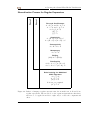
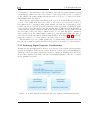
Normalizing Regular Expressions A systematic approach needs to be specified with
respect to the order, in which the transformation rules are to be performed on the
regular expression. The approach pursued here is illustrated in Figure 4.4. which will
be discussed in more detail in the remainder of this section.
First of all, it makes sense to distinguish between the transformation rules that involve
the three basic operations, which are part of the formally defined algebra for regular
expressions, namely concatenation, alternation and star, and those that were additionally
introduced as mere syntactic sugar, which were plus and optional. Equally, the process
of performing these transformations on a given regular expression in order to reduce it to
its normal form can be organized in two phases, where the former set of rules is applied
until the regular expression cannot be simplified any more in the first phase, before the
latter set of rules comes also to use in the second phase.
The reason for protracting the application of the additional operators on the regular
expression to be normalized can be best illustrated by example: Let +A+A be a regular
expression, which is clearly non-minimal. Either the alternation operator is assumed
to be left-associative, such that the expression becomes ( + A) + A = (A)? + A, or
the operator is assumed to be right-associative, in which case the duplicate expression
A would be eliminated first by the idempotency property before doing anything else,
resulting in + (A + A) = + A = (A)?. Implementing backtracking would be too
much of a hassle. Hence, the two-phase normalization process is the best solution to
prevent that a suboptimal result is delivered due to premature application of the plus
and optional operators.
The order, in which the transformation rules for the concatenation, alternation and
star operators are to be applied in the first phase, is specified like so:
Zero and One Elements: The rules that eliminate the zero and one elements in a regular
expression operate locally and therefore can be applied without consideration for
associativity and commutativity. For instance, for the regular expression A·∅·B the
result obtained after simplifying the same-operator sequence is the same no matter
how the operands are associated with the operators, such that (A·∅)·B = ∅·B = ∅
or A · (∅ · B) = A · ∅ = ∅.
Associativity: Associativity defines in what order the binary operators of same precedence are evaluated in the absence of parentheses in regular expressions. This is not
so much a simplification as a supportive means for normalizing the regular expres-
31
4 Creating the Control Flow Blocks Visualization
Phase 1
Phase 2
Normalization Process for Regular Expressions
Zero and One Elements
→
→
A + ∅ = A and ∅ + A = A
→
→
A · = A and · A = A
→
A·∅=∅·A=∅
→
∗
(∅) = →
()∗ = Associativity
→
A · (B · C) = (A · B) · C
→
A + (B + C) = (A + B) + C
Commutativity
→
A+B =B+A
Idempotency
→
A+A=A
Shifting
→
(AB)∗ A = A(BA)∗
Distributivity
→
A · B + A · C = A · (B + C)
→
A · C + B · C = (A + B) · C
Rules Involving the Additional
UNIX Operators
→
A + = A?
→
A · A∗ = A+
→ ∗
∗
(A?) = A
If A is not a terminal:
→
(A+ )? = A∗
Figure 4.4: Rules for bringing a regular expression into the normal form. A, B and C are
regular expressions. The arrows above the equation signs indicate that these
rules are to be applied from left to right only to reduce the computational
effort.
32
4.2 Normalization of Regular Expressions
sion in order to make more complex transformation rules easily applicable later on.
One can choose between left-associativity, where the operands are grouped starting from the left, and right-associativity, where the operands are grouped from the
right. Here, left-associativity shall be assumed [7].
Commutativity: Commutativity is similar to the associativity property in that it normalizes the regular expression to prepare it for subsequent simplification easier.
The operands of an operator with that property can be switched in their order
without having any effects on the result. In the algebra of regular expressions,
commutativity is only defined for the alternation and not the concatenation operator. Ultimately, how the operands are ordered in an alternation is an arbitrary
choice to be made. Here, the regular expressions are defined over the identifiers of
a deterministic finite automaton’s states. Hence, sorting these regular expressions
in ascending order with respect to their initial characters suggests itself.
The occurrence of an in the regular expressions is a special case that needs to
be treated separately. Because the alternation is evaluated from left to right as
specified with the associativity property and because rewriting it as an optional
should be done in the second phase after it has been fully simplified otherwise, all
occurrences are moved to the rightmost positions.
Idempotency: Having ordered the operands in an alternation, the detection of duplicate sub-expressions becomes easy: It only necessitates checking the immediate
neighbors of each operand within the alternation.
Shifting: The shifting rule is also not for the purpose of simplifying a regular expression
but, again, for achieving its normalization.
Distributivity: The distributive laws are to be applied last after the regular expression
has been fully normalized in accordance to the previous steps. Then, similar to the
idempotency property, the decision on whether the requirements for applying the
distributive laws on an alternation are met, can be simply made by only looking
at the immediate neighbors of each operand.
In the second phase, the additionally introduced quantifiers, namely the optional and
plus operators, come finally to use. Unlike the concatenation, alternation and star
operators, which are part of the algebra of regular expressions, the application of the
optional and plus operators to a regular expression does not affect the set of strings that
it accepts. Still, they allow to further minimize a regular expression like so:
→
A + = A?
∗ →
A · A = A+
∗ →
(A?) = A
→
∗
(A+ )? = A∗ if A is not a basic block
(4.1)
(4.2)
(4.3)
(4.4)
33
4 Creating the Control Flow Blocks Visualization
The regular expressions on the right-hand sides of the transformation rules above
describe sub-expressions that can occur in the regular expression computed for a control
flow graph. here exist equivalent regular expressions that can describe these patterns in
a more concise way.
The transformation rule in (4.1) denotes the case, where the control flow can be passed
on from one basic block to the other either directly or by taking a detour over other
basic blocks in the control flow graph. The execution of the detour can be indicated to
be optional in the respective regular expression using the optional operator. Because
of the transformations performed on the regular expressions in the first phase of the
normalization process, only alternations, in which the is the last operand, are considered
in this transformation rule.
Any basic block in a control flow graph that lies on an execution path has the chance
of being executed once, if that path is taken during program execution. If the basic block
has a self-loop as well, then that basic block might be executed more than once, when
the control flow reaches it. This case relates to the transformation rule in (4.2), where
the regular expression on the right-hand side is what usually results from the derivation
of a regular expression for the described control flow graph pattern. However, the same
semantics can be expressed by using the plus operator, which effectively eliminates the
basic block duplication and shortens the regular expression as a whole.
Both (4.3) and (4.4) are transformations that have proven themselves to be necessary in minimizing the regular expressions that were produced computationally using
the transitive closure method or Brzozowski’s method. Among all the possibilities of
combining or nesting the whole set of regular expression operators, these are the ones
that actually have a chance of occurring in a regular expression created for capturing
the control flow information of a control flow graph.
This list of transformation rules are applied, in addition to the ones used in the first
phase, to a given regular expression in the second phase of the normalization process.
34
4.3 Weakening of Regular Expressions
4.3 Weakening of Regular Expressions
Normalizing the regular expression as much as possible does not always yield a regular
expression, where each basic block only occurs once. When dealing with control flow
graphs with rather strongly connected components, chances are high that certain basic
blocks appear multiple times in the computed regular expression. This so-called basic
block duplication is a problem, because it causes the compactness of the control flow
blocks visualization to be reduced considerably.
Basic block duplication seems to occur whenever a node can be associated to at least
two control flow graph patterns simultaneously from among all possible patterns, as
shown in Figure 2.2, except for the one corresponding to sequential execution.
A
(a · b)+ · c · (d + d · e + e) · f
⇔ (a · b)+ · c · (d · ( + e) + e) · f
B
⇔ (a · b)+ · c · (d · (e)? + e) · f
C
D
⇒ (a · b)+ · c · (d · (e)? + (e)?) · f
E
⇒ (a · b)+ · c · (d + ) · (e)? · f
⇒ (a · b)+ · c · (d)? · (e)? · f
F
L((a · b)+ · c · (d + d · e + e) · f ) ⊂ L((a · b)+ · c · (d)? · (e)? · f )
Figure 4.5: An example of a regular expression for a control flow graph with basic block
duplication, which has been minimized by allowing it to become inaccurate.
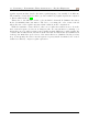
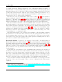
Figure 4.5 confirms that this suspicion is not unfounded like so: The example of a
control flow graph shown above yields a regular expression with basic block duplication.
Upon closer examination, it can be seen that it is the working example that has been
employed thus far (see Figure 2.1). However, it has been slightly modifed to include an
additional edge between the nodes D and E. This makes the node D associable with
two if-else patterns, of which one appears to have D as a possible targets while D is the
node, where the jump condition is evaluated, in the other. The regular expression that
captures all the control flow information is shown next to the graph. Despite applying
the rules for distributivity and optionalization to the regular expression to simplify it,
basic block duplication still persists because of e.
35
4 Creating the Control Flow Blocks Visualization
If the optional operator were to be applied to both of its occurrences, it would be
possible to again apply the rules for distributivity and optionalization in this order
resulting in a minimal regular expression, in which every basic block only appears once.
However, there is a side-effect to the replacement of e by (e)?: It causes the regular
expression to become inaccurate, such that the language now includes strings that were
originally not part of it. In other words, the regular expression that we started with
and the one that we end up with are not equivalent. At which point this happens in
the sequence of transformations performed on the regular expression is indicated in the
figure by the change from ⇔ to ⇒ as well as the use of a squiggled line.
In relation to the control flow graph, the inaccuracy in the regular expression makes
it seem as if there is an execution path, when there is actually none. According to the
inaccurate expression, the path passing through the nodes A, B, C, F in the mentioned
order is legal. A quick glance at the control flow graph proves otherwise.
Allowing the regular expression to be less accurate in order to reduce basic block
duplication improves the control flow visualization by a lot. We call this the weakening
of a regular expression. As long as no control flow information contained in the original
regular expression is lost, it is a very acceptable trade-off.
Currently, there are a total of four weakening rules. The case from the introductory
example constitutes the first weakening rule. Within the process of generating the control
flow blocks visualization, these rules are to be applied directly after the regular expression
has been normalized and right before the mapping to the control flow blocks takes place.
The reason for this is that, in order to decide whether a transformation of a regular
expression based on the proposed weakening rules is to be performed, a “global view
of the world” is necessary. Furthermore, it is not possible to undo the changes in the
regular expression that have been induced by the weakening rules.
How these weakening rules can be derived is discussed in detail in what follows to
show that nothing unintended happens. The following equivalence transformations from
Figure 3.3, where A, B and C denote regular expressions, are used:
A·=·A=A
(4.5)
A + = + A = A?
(4.6)
∗
A·A =A
+
(4.7)
A · B + A · C = A · (B + C)
(4.8)
A · C + B · C = (A + B) · C
(4.9)
(4.10)
Note that some of the rules mentioned above are made use of bidirectionally to conduct
the proofs. In addition, the use of these two transformations, which form the basis for
the weakening of regular expressions, is accepted:
36
⇒ A?
(4.11)
A ⇒ A?
(4.12)
4.3 Weakening of Regular Expressions
Both transformations yield regular expressions that accept more strings than the original
ones as results.
Weakening Rule 1 The first weakening rule is the one that was derived and discussed
in a detailed manner above. It is mentioned again here for the sake of completeness:
(a + a · b + b) ⇒ (a)? · (b)?
The corresponding control flow graph pattern is shown in Figure 4.6. Such a pattern
occurs, for instance, when a program contains an if-else statement, where a goto instruction in one of the two possible cases, whose execution depends on a condition, makes a
jump to the other case.
A
B
Figure 4.6: The control flow graph pattern underlying the first weakening rule.
In the normalization process, that was discussed earlier, the alternation operator has
been defined to be left-associative contrary to how it is used in the proof above. When
generating the control flow blocks visualization, the weakening rules are to be applied
to the regular expression after it has been simplified as much as possible. Therefore, the
pattern that a sub-expression needs to match for the rule to be applied to it is
(a + a · b) + b
(4.8)
⇐=⇒ a · ( + b) + b
(4.6)
⇐=⇒ a · (b)? + b,
hence, the weakening rule above needs to be adjusted like so:
a · (b)? + b ⇒ (a)? · (b)?.
Weakening Rule 2
The second weakening rule is:
a · (b · a)∗ ⇒ ((b)? · a)+
37
4 Creating the Control Flow Blocks Visualization
A
B
Figure 4.7: The control flow graph pattern underlying the second weakening rule.
The control flow pattern that underlies this transformation is one of the basic patterns,
namely the while-loop in Figure 4.7. The weakening rule can be derived as follows:
a · (b · a)∗
(4.5)
⇐=⇒ · a · (b · a)∗
(4.11)
==⇒ (b)? · a · (b · a)∗
(4.12)
==⇒ (b)? · a · ((b)? · a)∗
(4.7)
==⇒ ((b)? · a)+
The sub-expression a can be rewritten as the equivalent expression · a. The step
towards weakening the regular expression is done by replacing both and b by b + ,
which is (b)? for short. Once this is done, the whole regular expression can be simplified
by using the closure law involving the plus operator.
Like this, the basic block duplication caused by a can be eliminated at the cost of
allowing the resulting regular expression to accept illegal execution paths like B → A or
A → A → A → . . . and so on.
Weakening Rule 3
The third weakening rule is:
(a · c + b · c + b) ⇒ (a + b) · (c)?
Figure 4.8 illustrates the control flow graph pattern giving cause to the weakening
rule: A program resulting in such a pattern could contain an if-else statement, where
there is an if-statement in one of the two possible cases causing the called function to
return the control flow to the caller function in case that it evaluates to true. Otherwise,
the program keeps running until it completes its computation before the control flow
finally returns to the caller.
38
4.3 Weakening of Regular Expressions
A
B
C
Figure 4.8: The control flow graph pattern underlying the third weakening rule.
The proof, which shows that this rule is legit, goes as follows:
(a · c + b · c + b)
(4.8)
⇐=⇒ (a · c + b · (c + ))
(4.6)
⇐=⇒ (a · c + b · (c)?)
(4.12)
==⇒ (a · (c)? + b · (c)?)
(4.9)
==⇒ (a + b) · (c)?
First, the distributive law is applied to the two rightmost operands in the sameoperator sequence, after which the sub-expression c + is shortened to (c)?. In order to
be able to eliminate the surplus occurrence of c by applying the distributive law again,
all c’s in the regular expression need to be optionalized and this causes the regular
expression to become less accurate. For example, the weakened regular expression now
implies that there are execution paths going through only A or only B, but in fact these
paths do not exist in the control flow graph.
For the same reasons as above, the weakening rule needs to be adjusted to fit into the
whole transformation process, where the alternation operator is set to be left-associative,
such that
(4.9)
(a · c + b · c + b) ⇐=⇒ ((a + b) · c + b)
is pattern that is looked for in the regular expression for the following transformation to
be applied:
((a + b) · c + b) ⇒ (a + b) · (c)?.
Weakening Rule 4
The third weakening rule is as follows:
(a · b + a · c + c) ⇒ (a)? · (b + c)
A control flow graph can contain the pattern in Figure 4.9 described by the left-hand
side of the rule, if there are, for instance, two consecutive if-else statements, where one
case of one if-else statement can jump to the code executed in one case of the other via
a goto-statement.
39
4 Creating the Control Flow Blocks Visualization
A
B
C
Figure 4.9: The control flow graph pattern underlying the fourth weakening rule.
This weakening rule can be verified as follows:
(a · b + a · c + c)
(4.9)
⇐=⇒ (a · b + (a + ) · c)
(4.6)
⇐=⇒ (a · b + (a)? · c)
(4.12)
==⇒ ((a)? · b + (a)? · c)
(4.8)
==⇒ (a)? · (b + c)
The regular expression corresponding to this control flow graph pattern can be transformed much the same as it has been done in the proof for the third weakening rule.
Again, the weakening rule needs to be slightly adjusted to the visualization generation
process like so:
(a · (b + c) + c) ⇒ (a)? · (b + c).
40
5 Tool Implementation
For the purpose of testing the idea of control flow blocks, a prototype was implemented
that produces the envisioned visualization as output given a control flow graph as input.
How the concepts and methods presented until now work together in this tool and how
they are implemented is explained in this chapter.
5.1 General
The following components of .NET, which is an extensive framework for software development and execution developed by Microsoft, were used in the implementation of the
control flow visualization tool:
C# is a programming language that offers a very helpful feature, which is reflection.
Programs using reflection are able to examine their own metadata for some information,
based on which program execution can be modified at runtime. This feature will turn out
to be very helpful when implementing the functionality for normalizing and weakening
regular expressions.
LINQ (short for Language Integrated Query) extends C# by data querying capabilities
and is especially useful when used in a program in combination with collections of data
objects. LINQ allows to do what would take complex nested loop constructs otherwise
with the help of concise SQL-like queries.
WPF (short for Windows Presentation Foundation) is an API for creating graphical
user interfaces. It offers a set of standard controls to build a user interface with, which
are highly customizable. It is also possible to extend WPF by third-party controls.
5.2 Front End
This section gives an overview of the tool’s graphical user interface, of which a snapshot
is shown in Figure 5.1. It is designed to be clear in its structure: Much of the interface
area is designated to rendering the different program outputs, each of which is displayed
in a separate resizeable and dockable panel. A bar on the right offers the possibility to
access the hidden panels. A menu bar at the top, which is organized in tabs, provides
the user with options for loading the input control flow graph or for changing settings
concerning the process of generating the control flow blocks visualization.
Settings The interface allows the user to specify the settings, based on which the
control flow blocks visualization should be computed. The user can decide on whether
the regular expression that is to capture the control flow information contained in the
41
5 Tool Implementation
Figure 5.1: A snapshot of the user interface.
graph should be computed by means of the transitive closure method or Brzozowski’s
method and whether the weakening rules should be performed on the resulting regular
expression. Any change to these settings requires the input to be loaded again and the
outputs to be recomputed for the interface to be updated. In addition, the orientation
of the generated control flow block visualization, and the enabled scrolling direction for
that matter, can be changed from horizontal to vertical and vice versa. Per default, the
transitive closure is the method used to derive the regular expression, no weakening of
that regular expression takes place and the control flow blocks are aligned from left to
right in the visualization.
Input The tool accepts files with the extension .gdl, which contain textual representations of control flow graphs in Graph Description Language (GDL). IDA is a reverse
engineering tool for disassembling machine code and is capable of exporting a control
flow graph, there it is referred to as a flowchart, to such a file.
Output The tool produces multiple outputs. These are displayed in different panels:
Apart from the CFB Viewer, which is the panel displaying the control flow blocks visualization, there is also a CFG Viewer panel for viewing the input control flow graph and
a RE Tree Viewer showing the tree representation of the computed regular expression.
The multiple views are supported mainly for debugging purposes.
42
5.3 Back End
5.3 Back End
This section presents the implementation details relating to how the tool creates the
control flow blocks visualization from a control flow graph that is given as input. An
overview over the workflow, which also constitutes the roadmap that is followed in this
section, is shown in Figure 5.2.
Figure 5.2: Workflow for the generation of the control flow blocks visualization.
The workflow can be divided into four steps, some of which overlap: The process
starts with the creation of a data object from the textual specification of the control
flow graph contained in the input file. Then, a regular expression that represents the
whole set of possible execution paths within this control flow graph is derived. As can
be seen in the figure, this is actually done in two substeps, where the first converts the
control flow graph into a deterministic finite automaton and the second constructs a
regular expression that is equivalent to that automaton. The first phase of the transformation process runs in parallel to the construction process, whereas the second phase
runs at the end of it. The execution of the final phase of the transformation process,
which is the weakening of the regular expression, is either performed in the next step or
skipped entirely depending on the user’s choice. In the final step, the control flow blocks
visualization is generated for the regular expression, which is then displayed on the user
interface. These steps are explained in more detail in the following subsections.
5.3.1 Deserializing the Control Flow Graph
The textual representation of the control flow graph needs to be processed in order to
create an object that the tool can work with. A GDL parser that does exactly this has
been implemented by my supervisor, such that only the source and target representations
of this conversion are presented in a brief manner in what follows.
Graph Description Language GDL is a format originally developed for the use with
the graph visualization tool aiSee by AbsInt. It is very extensive in that it provides
many options for manipulating, for instance, the layout of a graph to be visualized on
screen among other details of its appearance. Here, however, only those parts of GDL
that come into use with IDA will be covered. For more information please refer to the
manual in [12].
43
5 Tool Implementation
hgraphi
::= graph: {
hgraph attributesi
hnodesi
hedgesi
}
hgraph attributesi
::= title: hstringi
manhattan_edges: yes
layoutalgorithm: mindepth
finetuning: no
layout_downfactor: 100
layout_upfactor: 0
layout_nearfactor: 0
xlspace: 12
yspace: 30
...
\\ Palette of colors used in IDA
...
hnodesi
::= hnodei hnodesi | hnodei
hedgesi
::= hedgei hedgesi | hedgei
hnodei
::= node: {
title: ‘‘hinti’’
label: hstringi
vertical_order: hinti
color: henumi
}
hedgei
::= edge: {
sourcename: ‘‘hinti’’
targetname: ‘‘hinti’’
label: hstringi
color: henumi
}
Figure 5.3: Grammar describing the structure of a GDL file produced with IDA.
44
5.3 Back End
Figure 5.3 provides a description of the general structure of GDL files generated for
control flow graphs with IDA. The textual representation of the graph can roughly be
distinguished into the following three parts:
Graph Attributes: The first part purely consists of graph attributes specifying the layout
of the graph visualization and the palette of colors that are to be used in it. IDA
adds this part with the same attribute values per default to each produced GDL
file. These attribute values are recommended in the aiSee manual for making the
graphs look like typical control flow graphs. However, the information contained
in this part is irrelevant for the purpose pursued here: In order to compute the
control flow blocks visualization it is necessary to know about the basic blocks and
the flow of control between them.
Nodes: The second part lists the nodes of the control flow graph. Each node has the
two mandatory attributes title and label; the latter contains the assembly instructions of the basic block that the node represents in form of a string, while the
former is the node’s unique numerical identifier. The nodes of the graph are listed
in the GDL file in ascending order of their identifiers. Information on how exactly
the numbers are assigned to the nodes is not available. Judging from example
GDL files, depth-first search (DFS) seems to be a pretty close guess.
The information about whether a node is either an entry point or an exit point
in the control flow graph is given with the attribute vertical order. In case the
node is an entry point this attribute is assigned the value 0. If the node is an
exit point, however, the vertical order is equal to the highest numerical identifier
assigned to a node within the control flow graph incremented by one. Optionally,
there is an attribute for setting the background color of the node in the graph
visualization.
Edges: The third part in the GDL file contains the edges. A directed edge is specified
by its adjacent nodes. The title of the source node of an edge is assigned to the
attribute sourcename, whereas the title of the target node of an edge is assigned
to the attribute targetname. In the file, the entries for the edges are sorted by
the sourcename attribute in ascending order. In case of an if-else pattern in the
control flow graph, the optional label and color attributes come to use: The
label is a Boolean value. Each possible Boolean value annotates one of the two
edges originating from the basic block, where the condition is evaluated. An edge
is traversed if the evaluation of the condition yields a Boolean value matching its
label. The edge labeled with true is assigned the color value green, the other
edge has the color value red.
Control Flow Graph Figure 5.4 is a class diagram illustrating the structure and the
main components of the CFG object created from the textual specification of the control
flow graph. Knowing about the nodes and the edges of the control flow graph is all
45
5 Tool Implementation
Figure 5.4: UML class diagram depicting what the data object representing the control
flow graph looks like.
that is needed to create the control flow blocks visualization. The class Node has the
attributes Title, which is assigned the numerical identifier of an instance in string form,
Label with the sequence of instructions in assembly language forming a basic block,
and Weight, which is basically the value that was assigned to the optional vertical
order attribute in the textual representation of the node. Meanwhile, the class Edge
provides the properties From and To to specify the source and target nodes of its instances
respectively.
5.3.2 Deriving a Regular Expression for the Control Flow Graph
This subsection deals with the derivation of a regular expression for the legal execution
paths of a control flow graph. Generally speaking, the process consists of two steps: The
first is concerned with transforming the control flow graph into a deterministic finite
automaton and the second is about computing the equivalent regular expression for this
automaton.
The user can choose between two methods for performing the latter step, either the
transitive closure method or Brzozowski’s method. The mathematics behind these methods were treated in Section 3.3 and it turned out that each method requires a slightly
different representation of the deterministic finite automaton for doing the computations. Therefore, the former step faces the task of offering the automaton in a form that
the method chosen by the user can work with.
Before discussing further implementation details for these methods, the data structure
used to represent the regular expressions will be treated first.
46
5.3 Back End
Figure 5.5: The class diagram for the implemented regular expression object hierarchy.
Regular Expression Regular expressions are implemented as object hierarchies. The
underlying class hierarchy is illustrated in Figure 5.5.
The regular expression operators are modeled by a class each. The alphabet, over
which a regular expression is defined, is comprised of instances of the Terminal class.
In most cases, these are wrappers around the nodes of the input control flow graph.
Exceptions are the Terminal objects representing the empty set constant ∅ and the
empty string constant . All these classes implement the interface IRegularExpression.
A more complex regular expression object can be constructed in terms of other regular
expression objects. It is best to think of a regular expression as a tree: All leaf nodes are
the elements of the alphabet, while all other nodes in the tree correspond to the regular
expression operators.
The arity of an operator is reflected in the number of properties in the respective
class, which are of type IRegularExpression and are referred to as children of the
operation. The Concatenation and Alternation objects are instantiated taking two
regular expressions as arguments, whereas the instances of the Star, Plus and Optional
can only have one regular expression object as child.
Transitive Closure Method The transitive closure method in itself is pretty straightforward to implement. Algorithm 1 provides a blueprint for the implementation and will
be discussed in what follows.1
The algorithm can be divided roughly into two parts: The lines 5 to 23 are responsible
for turning the input control flow graph into a deterministic finite automaton, whereas
the lines 25 to 38 compute a regular expression for that automaton.
R is the transition matrix of the deterministic finite automaton and its entries are to
1
The implementation of the transitive closure method is based on an algorithm posted online on stackexchange, which can be found under following link: http://cs.stackexchange.com/questions/2016/
how-to-convert-finite-automata-to-regular-expressions.
47
5 Tool Implementation
Algorithm 1 Transitive Closure Method
1: procedure TransitiveClosure(cf g)
2:
n ← number of nodes in cf g.N odes
3:
R ← square matrix over regular expressions of order n + 1
4:
5:
6:
7:
8:
9:
10:
11:
12:
13:
14:
15:
16:
17:
18:
19:
20:
21:
22:
23:
24:
25:
26:
27:
28:
29:
30:
31:
32:
33:
34:
35:
36:
37:
38:
39:
48
. (CFG → DFA)
for i ← 0, n do
for j ← 0, n do
if i equals j then
R[i, j] ← else
R[i, j] ← ∅
end if
end for
end for
for i ← 0, n − 1 do
if node i is an entry block in cf g then
R[0, i + 1] ← R[0, i + 1]+ node i
end if
for j ← 0, n − 1 do
if there is an edge from node i to node j ∈ cf g.Edges then
R[i + 1, j + 1] ← R[i + 1, j + 1]+ node j
end if
end for
end for
. (DFA → RE)
for k ← 0, n do
temp ← copy of R
for i ← 0, n do
for j ← 0, n do
R[i, j] ← temp[i, j] + temp[i, k] · (temp[k, k])∗ · temp[k, j]
end for
end for
end for
regexp ← ∅
for j ← 0, n − 1 do
if state j corresponds to an exit block in cf g then
regexp ← regexp + R[0, j + 1]
end if
end for
end procedure
5.3 Back End
be regular expressions. When specifying the order of this square matrix, the number of
its states has to be known, which is the count of nodes n in the control flow graph plus a
start state that needs to be introduced. The row and column in R at index 0 correspond
to this newly added start state, while all other rows and columns represent the nodes of
the control flow graph. A node with the numerical identifier k, where 0 ≤ k ≤ n − 1, is
represented by the k + 1-th row and column in R.
The first part of the algorithm fills R with entries: In lines 5 to 13, R is initialized
first by setting all entries to ∅ except for the entries on the diagonal, all of which is
assigned to. The lines from 14 to 23 link the start state to all states representing an
entry block. Moreover, the labels of the transition edges, which are Terminal objects
wrapped around the nodes of the control flow graph, are added to the entries in R.
Once the transition matrix R of the deterministic finite automaton has been built,
the actual transitive closure method is applied to it in the second part of the algorithm.
The regular expression equivalent to the automaton is computed inductively: In each
of the n + 1 iterations performed from line 25 to 32, a state of the deterministic finite
automaton is eliminated and the remaining transition edges are updated to include
that state’s behaviour. The elimination of the states occurs in increasing order of the
corresponding row or column index in R.
After all iterations have been performed, the remainder of the algorithm constructs
the alternation over all entries in R, which describe the paths from the start state of
the deterministic finite automaton to any of its final states. The latter represent the
exit blocks of the control flow graph. The regular expression resulting from the whole
procedure is contained in the variable regexp.
Brzozowski’s Method Compared to the transitive closure method, the implementation
Brzozowski’s method is a little cumbersome.2 The general structure of the underlying
algorithm, which is shown in Algorithm 2, remains the same: The transformation of the
input control flow graph to a deterministic finite automaton happens in lines 6 to 26,
while the conversion of the automaton to an equivalent regular expression takes place
in the remainder of the algorithm. In what follows, the algorithm will be examined in a
detailed manner.
As far as the the representation of the deterministic finite automaton is concerned, it
is different from how it was done in the transitive closure method in that two arrays are
necessary to model the characteristic equations, the square matrix A and the vector B.
The order of A and the length of B are equal to the number of nodes of the input control
flow graph incremented by one, which in turn equals the number of states that results
from the conversion of that control flow graph to a deterministic finite automaton.
A is pretty much a transition matrix: Its entries are Terminal objects wrapped around
the nodes of the control flow graph. These occur as coefficients in the characteristic
equations.
2
The implementation of Brzozowski’s method is based on an algorithm posted online on stackexchange, which can be found under following link: http://cs.stackexchange.com/questions/2016/
how-to-convert-finite-automata-to-regular-expressions.
49
5 Tool Implementation
Algorithm 2 Brzozowski’s Method
1: procedure Brzozowski(cf g)
2:
n ← number of nodes in cf g.N odes
3:
A ← square matrix over regular expressions of order n + 1
4:
B ← vector over regular expressions of length n + 1
5:
. (CFG → DFA)
6:
for i ← 0, n do
for j ← 0, n do
A[i, j] ← ∅
end for
B[i] ← ∅
end for
for i ← 0, n − 1 do
if node i represents an entry block then
A[0, i + 1] ← node i
end if
if node i represents an exit block then
B[i + 1] ← end if
end for
for i ← 0, n − 1 do
for j ← 0, n − 1 do
if there is an edge from node i to node j ∈ cf g.Edges then
A[i + 1, j + 1] ← node j
end if
end for
end for
. (DFA → RE)
for k ← n, 0 do
B[k] ← (A[k, k])∗ · B[k]
for j ← 0, k − 1 do
A[k, j] ← (A[k, k])∗ · A[k, j]
end for
for i ← 0, k − 1 do
B[i] ← B[i] + A[i, k] · B[k]
for j ← 0, k − 1 do
A[i, j] ← A[i, j] + A[i, k] · A[k, j]
end for
end for
for i ← 0, k − 1 do
A[i, k] ← ∅
end for
end for
end procedure
7:
8:
9:
10:
11:
12:
13:
14:
15:
16:
17:
18:
19:
20:
21:
22:
23:
24:
25:
26:
27:
28:
29:
30:
31:
32:
33:
34:
35:
36:
37:
38:
39:
40:
41:
42:
43:
50
5.3 Back End
Meanwhile, B will be a container for the regular expressions, which are obtained as
intermediate results. On initialization, an entry in the vector is set to , if the respective
node in the control flow graph is an exit block, otherwise it is set to ∅.
The part of the algorithm, which actually performs Brzozowski’s method spans the
lines 28 to 42. The states of the deterministic finite automaton are eliminated in descending order of their respective row or column index in A.
The elimination of a state k induces the characteristic equation Xk to be removed from
the system of characteristic equations that describe the deterministic finite automaton.
As such, it must be made sure that all occurrences of the unknown Xk on the righthand sides of all other characteristic equations are also removed. This is achieved by
substitution.
For the purpose of illustrating the effects of eliminating a state k on the data structures
A and B, let the following equation be the corresponding characteristic equation Xk :
Xk = A[k, 1] · X1 + · · · + A[k, k − 1] · Xk−1 + A[k, k] · Xk + B[k]
If the state k is to be eliminated, all states with a numerical identifier larger than k
must have already been eliminated according to how the algorithm is specified and their
behaviour must be covered by the regular expression B[k], which denotes all the input
strings that bring the deterministic finite automaton from state k to one of its final
states. This means that the characteristic equation of the state k can only depend on
the characteristic equations of the remaining states including itself.
If the unknown Xk appears on both sides of the equation, there is a self-loop at state
k in the deterministic finite automaton. This will pose a problem for the substitution
process later on. Applying Arden’s rule, which has been introduced in (3.2), to this
equation eliminates the self-loop and includes its behaviour in the regular expressions
that are the labels of all of its outgoing edges as follows:
Xk = (A[k, k])∗ · (A[k, 1] · X1 + · · · + A[k, k − 1] · Xk−1 + B[k])
Using the property of distributivity in reverse expands the right-hand side of the equation
like so:
Xk = (A[k, k])∗ · A[k, 1] · X1 + · · · + (A[k, k])∗ · A[k, k − 1] · Xk−1 + (A[k, k])∗ · B[k]
The resulting characteristic equation basically tells us how the entries in row k of the
matrix A and the entry k in the vector B need to be updated in accordance with Arden’s
rule: The expression (A[k, k])∗ is concatenated in front of all these entries, which is what
is done in line 29 to line 32.
The substitution process, which eliminates the occurences of the unknown Xk in all
other characteristic equations in the system, is mimicked in the algorithm by lines 34
to 36. The behaviour that will be lost due to the removal of the equation Xk from the
system, and hence the state k from the deterministic finite automaton, must be included
in all other equations.
The regular expressions in the transition matrix A describe all paths between any two
states i and j, where i, j ≤ k, and the ones in the vector B represent the paths from a
51
5 Tool Implementation
certain state i to the final states of the automaton. All of these regular expression entries
describing the paths from some source state to some target state need to be updated
to also include the paths passing through the state k, if k is to be removed from the
deterministic finite automaton.
There already exist regular expressions from a previous iteration that represent the
portion of the paths from any source state to the state k as well as the portion of
the paths from k to any target state in the matrix. As such, the concatenation of the
regular expressions of the two portions results in a regular expression describing the paths
between some source and target going through the state k. The subsequent alternation
of this with the regular expression entry in the arrays standing for the paths between
the very same source and target, which however do not pass through k, eliminates
all dependencies on the characteristic equation Xk and effectively makes the state k
removeable from the automaton. This is symbolically done in lines 39 to 41, where the
entries in column k + 1 corresponding to the state k are set to ∅.
The substitution process continues until only one characteristic expression is left. At
the end, the computed regular expression can be grabbed from the vector B at index 0.
5.3.3 Performing Regular Expression Transformations
In what follows, the implemented efforts to keep the size of the regular expressions manageable are discussed. Without any of these efforts the control flow blocks visualizations,
which are based on regular expressions, would be equally as unmanageable and hence
they would contribute very little to the the viewer’s understanding of the flow of control
in the visualized program.
Figure 5.6: A class diagram modeling the rule base with the transformations rules.
52
5.3 Back End
The Transformation Rules The tool contains a rule base specifying the allowed transformations on the regular expressions. The class diagram in Figure 5.6 shows how
exactly this has been implemented: Each rule is modeled as its own class. The set of
all implemented rules can be distinguished into two groups, one of which comprises the
normalization rules, while the other one is made up of the weakening rules. Depending on whether a rule is about normalizing or weakening, the class inherits from either
NormalizationRule or WeakeningRule respectively, both of which are abstract classes.
They, in turn, inherit from the abstract TransformationRule class.
The Transformation Function The process of transforming a regular expression is
outlined in Algorithm 3. Generally speaking, it is implemented as a recursive function.
In each recursion step, a subset of the transformation rules in the rule base is instantiated.
The rules in this subset are checked in a while-loop one by one for applicability to the
regular expression at hand. Whenever a rule is found to be applicable, it is applied.
After having checked all rules and possibly performed them on the regular expression,
the transformation process continues with the children of the regular expression in a
next recursion step. The number of children amounts to two at most, depending on the
operator object that is wrapped around them. Thinking of a regular expression as a tree
again, the recursion starts at the root of the tree and works its way all the way down to
the branches.
Once the recursion has reached the terminals, the recursive call returns. This completes one iteration of the while-loop. Before the while-loop can continue with the next
iteration, it checks whether the regular expression has changed in any way. If it indeed
did change, the next iteration of the while-loop is executed. Otherwise, it means that
none of the instantiated rules are applicable to the regular expression, upon which the
execution of the loop stops and the regular expression that has been transformed as
much as the implemented rules allow, is returned.
The whole transformation process is organized in three phases. The first two phases
perform equivalence transformations on the regular expressions following the two-phase
normalization procedure that was specified in Section 4.2. More specifically, the first
phase is concerned with applying the rules involving the concatenation, alternation and
star operators, while in the second phase, the rules involving the plus and optional
operators come in addition. The third and last phase in the transformation process is or
is not performed depending on the user’s choice. At this point all transformation rules
in the rule base, including the weakening rules proposed in Section 4.3, come to use.
The transformation rules are retrieved from the rule base by means of reflection, a
concept in C# which gives a program the ability to read its own metadata and to
modify its behavior accordingly while being executed. The metadata of a class includes,
for instance, information about its base classes. This proves itself to be useful: The
set of classes implementing the normalization rules, for example, can be filtered out
by searching for all classes in the assembly that inherit from NormalizationRule and
by instantiating them. The same goes for the retrieval of the weakening rules, except
that the result from the search in the assemby only encompasses those classes that
53
5 Tool Implementation
Algorithm 3 RE Transformation
1: procedure Transform(regexp, phase)
2:
rules ← rules instantiated from the rule base depending on phase
3:
clone ← null
4:
while regexp 6= clone do
5:
clone ← clone the regular expression regexp
6:
for all rules do
7:
if rule is applicable to regexp then
8:
regexp ← apply rule to regexp
9:
end if
10:
end for
11:
for all children of regexp do
12:
Transform(child, phase)
13:
end for
14:
end while
15: end procedure
are subclasses of WeakeningRule. However, this provides too weak of a distinction
considering that the set of normalization rules, which come to use in the first phase of
the transformation process, is only a subset of the set of all normalization rules existing
in the rule base. These are not applied in their entirety until the second phase of the
process is reached.
Each rule is assigned a weight to sort out, which rule is to be applied first in case
many are applicable to a regular expression. The smaller the weight of a rule, the higher
is its priority. Those rules that belong to the same grouping in Figure 4.4 have the same
weight value. Including the set of weakening rules, there are a total of eight priority
levels. The transformation rules involving the empty set ∅ or the empty string are of
highest priority, whereas the weakening rules are of lowest priority.
Apart from enforcing prioritization, the weights are also used to achieve a higher
degree of distinction when retrieving the rules: Apart from the regular expression to be
transformed, the Transform function obtains from the caller function an argument that
serves as an indicator for the phase the transformation process is currently in. With
that, the function looks up the subset of rules that are to be retrieved from the rule
base. The decision whether a rule from the rule base belongs to that subset is made
based on whether the weight that is assigned to it, lies within a certain range.
Applying the Transformation Fuction In the quest for deriving a regular expression
for the set of legal execution paths in a given control flow graph, both the transitive
closure method and Brzozowski’s method build in each iteration, more complex regular
expressions in terms of the ones created in a previous iteration. As such, the length of
the regular expressions degenerate rather quickly if no measures for simplifying them
are taken. To avoid that, it makes sense to simplify the regular expressions obtained as
intermediate results in the derivation process as much as possible from the get-go.
54
5.3 Back End
For starters, this is accomplished by inducing the first phase of the transformation
process with a call to the Transform function, whenever a new regular expression object
is constructed in the process of applying one of the methods mentioned above. Another
means to that end works one step ahead: Before even the constructor for creating
instances of the Concatenation class is called, checking whether any of the two regular
expressions that will be passed as arguments to the constructor are equal to the empty
set constant, avoids a lot of unnecessary computations.
The result is that the time and space requirements are effectively reduced. Also, it
becomes easier to comprehend the whole process of converting a control flow graph to a
regular expression.
A slight improvement of this result is achieved when the second phase of the transformation process is performed on the resulting regular expression, during which certain
sub-expressions are replaced by more concise expressions using the plus and optional
operators. As far as the weakening rules are concerned, they are applied lastly, once the
construction process is finished.
55
5 Tool Implementation
Figure 5.7: Outcome produced by the tool for the control flow graph from Figure 2.1.
5.4 Outcome
The output, which the implemented prototype produces for the control flow graph from
Figure 2.1 that has been used as working example throughout the thesis, is shown in
Figure 5.7. Actually, the output is comprised of three diagrammatic representations:
The first one is of the input control flow graph, which is displayed in the CFG Viewer
panel in the upper right corner. The second one, is a tree-like represention of the regular
expression that has been computed for the execution paths of the given control flow
graph. The regular expression shown in the RE Tree Viewer panel at the bottom right
is (0 · 1)∗ · 2 · (3 + 4) · 5. This is the same as the result obtained in Section 3.3 except that
the alphabet, over which the regular expression is defined, now consists of the numerical
identifiers of the nodes in the control flow graph instead of the previously used alphabetic
characters. The third and last one is the control flow blocks visualization in the CFB
Viewer panel on the left-hand side and looks exactly as expected when compared to
Figure 4.3. The same visualization is produced regardless of the method used to derive
to regular expression from the control flow graph and of whether the weakening rules
are applied or not.
The color scheme is kept consistent between these representations on purpose to illustrate the coherences.
56
6 Evaluation
There are requirements that the implemented prototype of the envisioned program visualization tool, and the underlying idea of control flow blocks for that matter, need to
meet.
The major concerns at the moment are not so much the time and memory it takes to
generate the control flow blocks visualization for a given control flow graph, though it
cannot be denied that they are of certain importance, as the correctness as well as the
usefulness of the produced results:
Correctness: The control flow blocks visualization is based on regular expressions. It
is the regular expression that contains the information about the flow of control
within a program in that it describes the set of all possible execution paths given in
the program’s control flow graph, which the tool takes as input. As such, it needs
to be made sure that the conversion of the input control flow graph into a regular
expression produces correct results. In addition, the resulting regular expression
needs to remain correct throughout any intermediate steps that are performed,
such as the normalization and weakening of that regular expression, until the
tool generates the control flow blocks visualization. The correctness requirement
also includes that all processes, which the regular expressions go through, deliver
outputs that are as expected. For instance, the normalization process should bring
a regular expression into the specified normal form.
Usefulness: Compared to correctness, the usefulness requirement is more about the
concept of control flow blocks than the implementation of the tool: Of course, the
use of the control flow blocks visualization needs to be perceived as beneficial by
the viewer, otherwise claiming it to be an alternative to the control flow graph
would not make much sense. This implies that the visualization needs to enhance
the viewer’s understanding of the program at least as much as a control flow graph.
To which extent these requirements actually met will be evaluated in the upcoming
chapter.
6.1 Correctness
The outcome of the tests, which were performed to ensure that the control flow blocks
visualizations generated by the tool are the results of correct computations, will be
discussed in this section.
Deserializing a GDL File The GDL parser goes beyond the scope of my own work.
Therefore, it is simply assumed that it has been sufficiently tested.
57
6 Evaluation
Transforming Regular Expressions As mentioned before, the process of generating a
regular expression for all execution paths in a given control flow graph and the first
phase of the transformation process are intertwined. As such, guaranteeing that all the
transformation rules in the rule base work the way they are expected to, will make it
easier to verify that the conversion of the control flow graph into a regular expression
yields correct results.
Unit tests were performed on the transformation rules in the rule base in order to check
that they have been implemented correctly: For each transformation rule and for every
base case, in which that particular transformation rule is applicable, a simple regular
expression object was constructed and passed as an argument to the transformation
function. The expected result was then checked for equality with the actual result of the
transformation. The unit test was passed successfully in case of equality.
Although the unit tests devised as sketched above were rather simple, they achieved
a relatively high test coverage as can be understood from Figure 6.1, with a little more
than 90% of the code covered.
Converting a Control Flow Graph to a Regular Expression Implementing two methods
for converting a control flow graph to a regular expression was rather for debugging
purposes than for giving the user of the tool the opportunity to configure the process.
Being able to compare the results produced for the same input control flow graph by
means of the two different methods has two advantages: Firstly, it might help when
assessing the correctness of these methods and, secondly, it shows whether the attempts
at normalizing the regular expressions have been successful.
The size of the control flow graphs used for testing were limited to at most twenty nodes
in order to render the construction process of the regular expression more trackable. The
test cases were randomly chosen from among IDA’s outputs.
For starters, the control flow graphs that are the simplest and smallest in terms of
the number of nodes they consist of, were chosen among all selected test cases. These
were used to check whether both the transitive closure method and Brzozowski’s method
yield regular expressions as results that correctly capture the control flow information,
which they indeed did.
As to whether the produced regular expressions are normalized, one can say that in
the majority of cases they are. For all other cases, two reasons can be identified as to
why the normalization process fails. These will be discussed detailedly in the following.
One reason for the semantic difference in the regular expressions produced by the
methods can be traced back to the difference in how these methods are implemented
to proceed when they eliminate the states of an deterministic finite automaton in the
process of producing an equivalent regular expression. The difference in the sequence of
state removals can result, as already mentioned, in different regular expressions for each
method.
The transitive closure method basically eliminates the states of the automaton in ascending order of their numerical identifiers. Without any simplification, the size of the
resulting regular expression explodes and the computational effort needed to construct
58
6.1 Correctness
Figure 6.1: Table showing the achieved code coverage with the unit tests performed on
the transformation rules.
59
6 Evaluation
it is also rather high [11]. However, such a regular expression can be brought easily into
its normal form as specified in Figure 4.4. By contrast, Brzozowski’s method removes
the states from the deterministic finite automaton in decreasing order of their numerical
identifiers and produces an equivalent regular expression that already is somewhat simplified [11]. Sometimes, this might prevent the regular expression from being convertible
to its normal form, because doing so requires the regular expression to be expanded
prior to normalizing it. However, this clashes with the unidirectional application of the
transformation rules during the transformation process.
A concrete example of how the order of state removal affects the generated regular
expression is shown in Figure 6.2. The figure presents a control flow graph, for which the
regular expressions were computed by means of the two available methods. Both regular
expressions are correct in that they capture the control flow information contained in the
control flow graph. However, the normalization process has only managed to bring the
one resulting from the transitive closure method into the defined normal form. Meanwhile, there is no way for the regular expression obtained with Brzozowski’s method to
be normalized with the currently available transformation rules in the rule base, since no
transformation rule for applying the distibutivity law in reverse is implemented. Such a
rule would be necessary to expand the regular expression before it can be brought into
the same form as the other result.
A
B
D
Transitive Closure
A · ((B + D) · C · F + D · E)
C
E
Brzozowski
A · (B · C · F + D · (C · F + E))
F
Figure 6.2: The regular expressions computed by the transitive closure method and Brzozowski’s method with cf ifelifret.gdl as input.
The other reason for why regular expressions computed by the methods for the same
control flow graph can differ, is the occurrence of cycles in that control flow graph, where
many of the nodes that are part of these cycles constitute exit points, through which
the control flow can leave.
A simple example of such a case is presented in Figure 6.3: The control flow graph has
a cycle going through the nodes B and D. The control flow enters this cycle through
B and can leave it through either B or D to reach the node C or E respectively. The
regular expressions on the right side of the control flow graph are the regular expression
60
6.1 Correctness
A
Transitive Closure
B
D
A · B · ((D · B)∗ · C + D · (B · D)∗ · E)
C
Brzozowski
E
A · B · (D · B)∗ · (C + D · E)
Figure 6.3: The regular expressions computed by the transitive closure method and Brzozowski’s method with strchr.gdl as input.
that have been computed for this control flow graph with the help of the two methods.
Again, it can be simply verified that both regular expressions represent the control flow
graph, although one would assume otherwise at first glance. The regular expression that
is the result of the transitive closure method is more complex than the one obtained with
Brzozowski’s method. If it were possible for the shifting rule to be applied bidrectionally
in the normalization process, the former expression could be transformed into the latter
like so:
A · B · ((D · B)∗ · C + D · (B · D)∗ · E)
⇔ A · B · ((D · B)∗ · C + (D · B)∗ · D · E)
⇔ A · B · (D · B)∗ · (C + D · E)
The shifting rule is applied in the first step, resulting in a regular expression, to which
then the distributivity law can be applied in the second step. This already completes the
reduction of the more complex regular expression to the simpler one. But as a matter
of fact, the rule base implemented in the tool does not include a transformation rule for
shifting in reverse, such that it is not possible with the current version of the tool to get
to this result.
The same observations can be made when using the more complex test cases, only that
the lack of normalization of the generated regular expressions makes it hard to check
them for correctness.
Generally, one can summarize the results of the tests by stating that the bigger the
input control flow graph is and the more interconnected its nodes are, the more difficult
it is to produce normalized regular expressions as results.
To the question as to whether the transitive closure method or Brzozowski’s method
is better, there is no definite answer as both work correctly, but not in a way that is
desirable for the control flow blocks visualization. For certain instances of control flow
graphs the transitive closure method yields better regular expressions, and for other
61
6 Evaluation
instances Brzozowski’s method might prove itself to be the better choice. At this point,
the transitive closure method seems to be the safer choice. However, what has become
apparent here is that trying to fit one normalization procedure to both methods, which
are clearly different in how they work to accomplish the same task, is a naive approach.
As for the weakening rules, due to the flaws in the normalization process there is not
enough common ground, which would allow for reliable statements about their success
to be made. For control flow graphs of manageable size they were at most proven doing
nothing unintended.
6.2 Usefulness
For the control flow blocks visualization to be considered useful, it needs to help a user
gain an understanding of the flow of control between a program’s basic blocks. Although
a thorough assessment of the usefulness of this alternative visualization actually necessitates experiments, where real users working with the developed software are observed,
this is work left for later due to time constraints.
For now, we restrict ourselves to discuss noticeable problems with the implemented
prototype of the envisioned visualization tool that impact the usefulness from the point
of view of a user, of which the following few were detected:
One problem is related to one of the additional views, namely the CFG Viewer, which
shows the input control flow graph. Graph# or GraphSharp 1 is a graphics library that
is used in the implementation to render the graph. But it seems to have issues with
rendering self-loops as they are not displayed at all. However, an alternative graphics
library could not be found.
Another problem is more of importance in that it concerns the control flow blocks
visualization: For control flow graphs that contain strongly connected components, the
control flow blocks visualizations become deeply nested and thus can be unintuitive to
understand. Although this can be put into perspective easily, since it is highly probable
that such control flow graphs by themselves are equally as unintuitive to understand, it
would be still good, if the tool could handle such complex control flow graphs.
Yet another problem has something to do with the weakening rules, which a user
can choose to let the tool perform on the regular expression that will be mapped to
the control flow visualization. Currently, there is no feedback for whether the selected
execution path in the control flow visualization is actually a legal path or not, in case
the regular expression has been indeed weakened. A possible solution is to synchronize
the control flow graph and the control flow blocks views on the user interface, such that
an execution path selected in one of the two views is also highlighted in the other.
1
Project website under: http://graphsharp.codeplex.com/
62
7 Conclusion and Future Work
The main purpose of this bachelor thesis was to introduce control flow blocks, a new
method for visualizing the control flow between the basic blocks of a program. It is based
on regular expressions defined over the basic blocks that serve as means for capturing
the control flow information contained in the control flow graphs. The set of regular
expression operators that are used, achieve the abstraction of the linkage into explicit
structures. These execution structures are then represented in the visualization by using
the visual property of containment. The result is an overlay of the execution paths, each
a sequence of basic blocks, where the execution structures around the basic blocks allow
to switch between the different paths.
A prototype of the envisioned program visualization tool was implemented that takes
the textual specification of a control flow graph in Graph Description Language as input
and produces the control flow blocks visualization as output to the screen. The process of
generating the visualization makes use of the equivalence of deterministic finite automata
to regular expressions in formal language theory and of the similarity of a control flow
graph to a deterministic finite automaton: The deserialized control flow graph is first
transformed into a deterministic finite automaton, after which an equivalent regular
expression is computed by means of either the transitive closure method or Brzozowski’s
method.
However, it turned out that these computational methods not only tend to create
very large regular expressions, but they also result in different regular expressions to be
computed for the same deterministic finite automaton due to the difference in the order,
in which states are eliminated in the process. In order to prevent this from affecting
the produced control flow blocks visualizations negatively, a normal form for the regular
expressions as well as a strategy to bring them into this normal form were defined. Also,
control flow graphs, where nodes are associable to more than two control flow graph
patterns, were found giving rise to regular expressions with basic block duplication. For
the sake of reducing basic block duplication and hence rendering the control flow blocks
visualizations more compact, transformations were allowed for weakening the accuracy
of regular expressions to an extent, which makes it possible to shorten them more. All in
all, a transformation process was implemented in the tool, in which normalization and
weakening are performed on the regular expressions in three phases.
The evaluation of the tool showed that the specified approach to normalizing the
regular expressions obtained with the two different methods is not really effective for
control flow graphs with strongly connected components. It was found that the inherent
difference in how they accomplish the task of deriving the regular expressions cannot
be overcome by one universal approach for such control flow graphs and that different
approaches geared to the inner workings of the respective method might yield better
results.
Apart from the problems that cropped up in relation to how the control flow blocks
visualizations are generated, there were also certain issues concerning the usability of
63
7 Conclusion and Future Work
the tool that might impact the usefulness of the visualization in a negative way. For
example, a mechanism that, in case the underlying regular expression underwent weakening, provides the user with feedback when an illegal execution path is selected in the
control flow blocks visualization is currently absent. Furthermore, it would be good if
a solution to reduce nestedness of the control flow blocks visualizations resulting from
complex control flow graphs were to be found.
Once the points that need improvement as mentioned above are dealt with, there are
certain matters that might be interesting to examine further.
The assessment of the usefulness of control flow blocks has not been done here thoroughly enough. It would be interesting to know to what extent using the tool enhances
the users’ understanding of the control flow in a program. For that purpose, a group of
test subjects could be observed solving problems involving some program function with
the help of its control flow graph and its control flow blocks visualization and asked for
their opinion on which one they find better. To avoid any bias towards the control flow
graph, it would be the best to pick first-year computer science students as test subjects,
because it can be assumed that they are not as conditioned to think in terms of control
flow graphs yet.
Also, it would be interesting to apply the concept of control flow blocks to program
functions written in high-level programming languages. Thus far, the visualization tool
has been tested with control flow graphs for functions specified in assembly language.
The low level of abstraction causes the control flow graphs to be rather complex in their
structure. A guess would be that functions specified in high-level programming languages
have a lower chance of degenerating into unmanageable control flow graphs. Therefore,
the problems that were faced here with the test cases might not be as pronounced.
Last but not least, the current form of the control flow blocks visualization could be
extended by a further aspect to be visualized: The data flow within the basic blocks could
be illustrated instead of showing the instructions. As a consequence, the visualization
would become totally independent of the underlying program code relieving the viewer
of having to read through it in order to understand the semantics.
These topics were left outside the scope of this work, but they give reason for future
work.
64
Bibliography
Bibliography
[1] S. Diehl, Software Visualization: Visualizing the Structure, Behaviour, and Evolution of Software. Secaucus, NJ, USA: Springer-Verlag New York, Inc., 2007.
[2] B. A. Price, R. M. Baecker, and I. S. Small, “A Principled Taxonomy of Software
Visualization,” Journal of Visual Languages & Computing, vol. 4, no. 3, pp. 211 –
266, 1993.
[3] K. Saleh, Software Engineering. J. Ross Pub., 2009.
[4] National Instruments, LabVIEW User Manual, April 2003.
[5] National Instruments, LabVIEW Fundamentals, August 2005.
[6] J. Kodosky, J. MacCrisken, and G. Rymar, “Visual Programming using Structured
Data Flow,” in Visual Languages, 1991., Proceedings. 1991 IEEE Workshop on,
pp. 34–39, 1991.
[7] J. E. Hopcroft and J. D. Ullman, Introduction To Automata Theory, Languages,
And Computation. Boston, MA, USA: Addison-Wesley Longman Publishing Co.,
Inc., 1st ed., 1990.
[8] J. E. Savage, Models of Computation: Exploring the Power of Computing. Boston,
MA, USA: Addison-Wesley Longman Publishing Co., Inc., 1st ed., 1997.
[9] J. A. Brzozowski, “Derivatives of Regular Expressions,” J. ACM, vol. 11, pp. 481–
494, Oct. 1964.
[10] R. Kain, Automata Theory: Machines and Language. McGraw-Hill computer science series, Krieger, 1972.
[11] C. Neumann, “Converting Deterministic Finite Automata to Regular Expressions,”
2005.
[12] AbsInt Angewandte Informatik GmbH, aiSee User Manual for Windows and Linux,
version 3.4.3 ed., December 2009.
65
List of Figures
List of Figures
2.1
2.2
2.3
2.4
2.5
2.6
An Example of a Control Flow Graph . . . . . . . .
Basic Control Flow Graph Patterns . . . . . . . . . .
An Example of a LabVIEW Virtual Instrument . . .
An Virtual Instrument using an Execution Structure
Execution Structures in LabVIEW . . . . . . . . . .
The variants of the LabVIEW Case Structure . . . .
.
.
.
.
.
.
.
.
.
.
.
.
.
.
.
.
.
.
.
.
.
.
.
.
.
.
.
.
.
.
.
.
.
.
.
.
.
.
.
.
.
.
4
5
6
8
9
9
3.1
3.2
3.3
3.4
3.5
3.6
An Example of a Deterministic Finite Automaton . . . . . . . . . . . . .
The Empty Set and Empty String in the Algebra of Regular Expressions .
Transformation Rules for Regular Expressions . . . . . . . . . . . . . . . .
Illustration of the Induction Step in the Transitive Closure Method . . . .
Applying Brzozowski’s Method . . . . . . . . . . . . . . . . . . . . . . . .
Setup for the Juxtaposition of the Conversion Methods . . . . . . . . . . .
12
14
17
19
21
22
4.1
4.2
4.3
4.4
4.5
4.6
4.7
4.8
4.9
Regular Expressions for the Basic Control Flow Graph
The Visual Language of Control Flow Blocks . . . . .
An Example of the Control Flow Blocks Visualization
The Normalization Process for Regular Expressions . .
An Example of Basic Block Duplication . . . . . . . .
The first Weakening Rule . . . . . . . . . . . . . . . .
The second Weakening Rule . . . . . . . . . . . . . . .
The third Weakening Rule . . . . . . . . . . . . . . . .
The fourth Weakening Rule . . . . . . . . . . . . . . .
.
.
.
.
.
.
.
.
.
.
.
.
.
.
.
.
.
.
.
.
.
.
.
.
.
.
.
.
.
.
.
.
.
.
.
.
.
.
.
.
.
.
.
.
.
27
29
29
32
35
37
38
39
40
5.1
5.2
5.3
5.4
5.5
5.6
5.7
A Snapshot of the Tool’s User Interface . . . . . . . . . . . . . . .
The Generation Process for the Control Flow Blocks Visualization
The Grammar of the Graph Description Language . . . . . . . . .
UML Class Diagram modeling Control Flow Graphs . . . . . . . .
UML Class Diagram modeling Regular Expressions . . . . . . . . .
UML Class Diagram modeling the Rule Base . . . . . . . . . . . .
The Control Flow Visualization For the Working Example . . . . .
.
.
.
.
.
.
.
.
.
.
.
.
.
.
.
.
.
.
.
.
.
.
.
.
.
.
.
.
42
43
44
46
47
52
56
6.1
6.2
6.3
Unit Testing the Transformation Rules . . . . . . . . . . . . . . . . . . . . 59
Regular Expressions produced for cf ifelifret.gdl . . . . . . . . . . . 60
Regular Expressions produced for strchr.gdl . . . . . . . . . . . . . . . 61
Patterns
. . . . .
. . . . .
. . . . .
. . . . .
. . . . .
. . . . .
. . . . .
. . . . .
.
.
.
.
.
.
.
.
.
.
.
.
.
.
.
.
.
.
.
.
.
.
.
.
.
.
.
.
.
.
.
.
.
.
.
.
.
.
.
67