Download Obstacle detection using V-disparity: Integration to the CRAB rover

Obstacle detection using V-disparity:
Integration to the CRAB rover
Matthias Wandfluh
Bachelor Thesis
Spring 09
Supervisors:
Professor:
Ambroise Krebs, Mark Höpflinger
Prof. Roland Siegwart, ASL
Autonomous Systems Lab
ETH Zürich
Abstract
The goal of this bachelor thesis is to integrate an existing obstacle detection algorithm
on the CRAB rover. The algorithm is based on v-disparity and was developed by
Christophe Chautems as a semester project during the autumn semester 2008 at the
Autonomous Systems Lab ETHZ. The existing algorithm was improved during this
work. As a result, the algorithm is successfully integrated to the CRAB rover and
adapted to the specifications of the robot. Furthermore an offline mode is programmed
in order to compare different settings. The obstacle maps are used to update an obstacle prediction grid, which provides the essential informations to avoid obstacles. The
software is tested using a simulation software as well as the CRAB rover. The main
ideas behind the implemented methods and the test results are presented in this work.
i
Contents
1. Introduction
1.1. State of the Art . . . . . . . . . . . . . . . . . . . . . . . . . . . . . . . .
1.2. Content . . . . . . . . . . . . . . . . . . . . . . . . . . . . . . . . . . . .
1
1
2
2. System overview
2.1. CRAB rover . . . . . . . . .
2.1.1. Design of the CRAB
2.1.2. Navigation module .
2.2. Stereo camera . . . . . . . .
2.2.1. General informations
2.2.2. Videre Design Stereo
2.2.3. SVS Software . . . .
. . . . .
. . . . .
. . . . .
. . . . .
. . . . .
Camera
. . . . .
.
.
.
.
.
.
.
.
.
.
.
.
.
.
.
.
.
.
.
.
.
.
.
.
.
.
.
.
.
.
.
.
.
.
.
.
.
.
.
.
.
.
.
.
.
.
.
.
.
.
.
.
.
.
.
.
.
.
.
.
.
.
.
.
.
.
.
.
.
.
.
.
.
.
.
.
.
.
.
.
.
.
.
.
.
.
.
.
.
.
.
.
.
.
.
.
.
.
.
.
.
.
.
.
.
.
.
.
.
.
.
.
.
.
.
.
.
.
.
.
.
.
.
.
.
.
.
.
.
.
.
.
.
.
.
.
.
.
.
.
3
3
3
4
6
6
8
9
3. Obstacle detection using stereo images
3.1. Obstacle detection algorithm . . . .
3.2. Improvements . . . . . . . . . . . . .
3.2.1. Image source . . . . . . . . .
3.2.2. Roll Detection . . . . . . . .
3.2.3. Rotate disparity . . . . . . .
3.2.4. Floor detection . . . . . . . .
3.2.5. Map blocks . . . . . . . . . .
3.3. Implementation . . . . . . . . . . . .
3.4. Performance . . . . . . . . . . . . . .
3.4.1. Disparity problem . . . . . .
.
.
.
.
.
.
.
.
.
.
.
.
.
.
.
.
.
.
.
.
.
.
.
.
.
.
.
.
.
.
.
.
.
.
.
.
.
.
.
.
.
.
.
.
.
.
.
.
.
.
.
.
.
.
.
.
.
.
.
.
.
.
.
.
.
.
.
.
.
.
.
.
.
.
.
.
.
.
.
.
.
.
.
.
.
.
.
.
.
.
.
.
.
.
.
.
.
.
.
.
.
.
.
.
.
.
.
.
.
.
.
.
.
.
.
.
.
.
.
.
.
.
.
.
.
.
.
.
.
.
.
.
.
.
.
.
.
.
.
.
.
.
.
.
.
.
.
.
.
.
.
.
.
.
.
.
.
.
.
.
.
.
.
.
.
.
.
.
.
.
.
.
.
.
.
.
.
.
.
.
.
.
.
.
.
.
.
.
.
.
.
.
.
.
.
.
.
.
.
.
11
11
13
14
14
15
17
17
18
19
21
4. Map handling
4.1. Different approaches . . . . . . . . . .
4.1.1. Add constant . . . . . . . . . .
4.1.2. Probabilistic approach . . . . .
4.1.3. Differential equation approach
4.1.4. Comparison . . . . . . . . . . .
4.2. Map building on the CRAB rover . . .
.
.
.
.
.
.
.
.
.
.
.
.
.
.
.
.
.
.
.
.
.
.
.
.
.
.
.
.
.
.
.
.
.
.
.
.
.
.
.
.
.
.
.
.
.
.
.
.
.
.
.
.
.
.
.
.
.
.
.
.
.
.
.
.
.
.
.
.
.
.
.
.
.
.
.
.
.
.
.
.
.
.
.
.
.
.
.
.
.
.
.
.
.
.
.
.
.
.
.
.
.
.
.
.
.
.
.
.
.
.
.
.
.
.
23
23
23
25
25
27
27
5. Simulation
5.1. Integration to Webots . . . . . . . . . . . . . . . . . . . . . . . . . . . .
35
35
6. Integration on the CRAB rover
41
iii
Contents
7. Test
7.1.
7.2.
7.3.
results on
Setup . .
Results . .
Summary
CRAB
. . . .
. . . .
. . . .
rover
. . . . . . . . . . . . . . . . . . . . . . . . . . . . . . .
. . . . . . . . . . . . . . . . . . . . . . . . . . . . . . .
. . . . . . . . . . . . . . . . . . . . . . . . . . . . . . .
43
43
44
46
8. Conclusion
49
A. Configuration files
55
B. CD content
61
C. Start manual
C.1. Installation . . . . . . . .
C.1.1. SVS . . . . . . . .
C.1.2. IPipeline . . . . .
C.1.3. Navigation . . . .
C.2. Run software . . . . . . .
C.2.1. Obstacle Detection
C.2.2. Other modules . .
iv
.
.
.
.
.
.
.
.
.
.
.
.
.
.
.
.
.
.
.
.
.
.
.
.
.
.
.
.
.
.
.
.
.
.
.
.
.
.
.
.
.
.
.
.
.
.
.
.
.
.
.
.
.
.
.
.
.
.
.
.
.
.
.
.
.
.
.
.
.
.
.
.
.
.
.
.
.
.
.
.
.
.
.
.
.
.
.
.
.
.
.
.
.
.
.
.
.
.
.
.
.
.
.
.
.
.
.
.
.
.
.
.
.
.
.
.
.
.
.
.
.
.
.
.
.
.
.
.
.
.
.
.
.
.
.
.
.
.
.
.
.
.
.
.
.
.
.
.
.
.
.
.
.
.
.
.
.
.
.
.
.
.
.
.
.
.
.
.
.
.
.
.
.
.
.
.
.
.
.
.
.
.
63
63
63
63
63
63
63
64
List of Figures
2.1.
2.2.
2.3.
2.4.
2.5.
2.6.
2.7.
2.8.
CRAB: Chassis . . . .
CRAB: Virtual wheel
CRAB: Modules . . .
Estar trace . . . . . .
Stereo camera buildup
Disparity function . .
Coordinate systems . .
STH-MDCS2-C . . . .
.
.
.
.
.
.
.
.
.
.
.
.
.
.
.
.
.
.
.
.
.
.
.
.
.
.
.
.
.
.
.
.
.
.
.
.
.
.
.
.
.
.
.
.
.
.
.
.
.
.
.
.
.
.
.
.
.
.
.
.
.
.
.
.
.
.
.
.
.
.
.
.
.
.
.
.
.
.
.
.
.
.
.
.
.
.
.
.
.
.
.
.
.
.
.
.
.
.
.
.
.
.
.
.
.
.
.
.
.
.
.
.
.
.
.
.
.
.
.
.
.
.
.
.
.
.
.
.
.
.
.
.
.
.
.
.
.
.
.
.
.
.
.
.
.
.
.
.
.
.
.
.
.
.
.
.
.
.
.
.
.
.
.
.
.
.
.
.
.
.
.
.
.
.
.
.
.
.
.
.
.
.
.
.
.
.
.
.
.
.
.
.
.
.
.
.
.
.
.
.
3
4
5
6
7
7
8
9
3.1.
3.2.
3.3.
3.4.
3.5.
3.6.
3.7.
Obstacle detection algorithm
Offline/online image source .
Image source . . . . . . . . .
Roll detection . . . . . . . . .
Rotate disparity . . . . . . .
V-disparity . . . . . . . . . .
Maps . . . . . . . . . . . . . .
.
.
.
.
.
.
.
.
.
.
.
.
.
.
.
.
.
.
.
.
.
.
.
.
.
.
.
.
.
.
.
.
.
.
.
.
.
.
.
.
.
.
.
.
.
.
.
.
.
.
.
.
.
.
.
.
.
.
.
.
.
.
.
.
.
.
.
.
.
.
.
.
.
.
.
.
.
.
.
.
.
.
.
.
.
.
.
.
.
.
.
.
.
.
.
.
.
.
.
.
.
.
.
.
.
.
.
.
.
.
.
.
.
.
.
.
.
.
.
.
.
.
.
.
.
.
.
.
.
.
.
.
.
.
.
.
.
.
.
.
.
.
.
.
.
.
.
.
.
.
.
.
.
.
.
.
.
.
.
.
.
.
.
.
.
.
.
.
12
14
15
16
16
17
19
4.1.
4.2.
4.3.
4.4.
4.5.
4.6.
4.7.
Add constant . . . . .
Probabilistic approach
Differential equation .
Dilate obstacles . . . .
Field of view . . . . .
Map sections . . . . .
Grids . . . . . . . . . .
.
.
.
.
.
.
.
.
.
.
.
.
.
.
.
.
.
.
.
.
.
.
.
.
.
.
.
.
.
.
.
.
.
.
.
.
.
.
.
.
.
.
.
.
.
.
.
.
.
.
.
.
.
.
.
.
.
.
.
.
.
.
.
.
.
.
.
.
.
.
.
.
.
.
.
.
.
.
.
.
.
.
.
.
.
.
.
.
.
.
.
.
.
.
.
.
.
.
.
.
.
.
.
.
.
.
.
.
.
.
.
.
.
.
.
.
.
.
.
.
.
.
.
.
.
.
.
.
.
.
.
.
.
.
.
.
.
.
.
.
.
.
.
.
.
.
.
.
.
.
.
.
.
.
.
.
.
.
.
.
.
.
.
.
.
.
.
.
.
.
.
.
.
.
.
.
.
.
.
.
.
.
.
.
.
.
.
.
.
.
.
.
.
.
.
.
24
26
27
29
31
31
32
5.1.
5.2.
5.3.
5.4.
Webots
Webots:
Webots:
Webots:
.
.
.
.
.
.
.
.
.
.
.
.
.
.
.
.
.
.
.
.
.
.
.
.
.
.
.
.
.
.
.
.
.
.
.
.
.
.
.
.
.
.
.
.
.
.
.
.
.
.
.
.
.
.
.
.
.
.
.
.
.
.
.
.
.
.
.
.
.
.
.
.
.
.
.
.
.
.
.
.
.
.
.
.
.
.
.
.
.
.
.
.
.
.
.
.
.
.
.
.
.
.
.
.
.
.
.
.
.
.
.
.
.
.
.
.
.
.
.
.
36
37
38
39
7.1.
7.2.
7.3.
7.4.
7.5.
STOC stereo camera
Test run . . . . . . .
Strange movements .
CRAB positions . .
Temporary goals . .
.
.
.
.
.
.
.
.
.
.
.
.
.
.
.
.
.
.
.
.
.
.
.
.
.
.
.
.
.
.
.
.
.
.
.
.
.
.
.
.
.
.
.
.
.
.
.
.
.
.
.
.
.
.
.
.
.
.
.
.
.
.
.
.
.
.
.
.
.
.
.
.
.
.
.
.
.
.
.
.
.
.
.
.
.
.
.
.
.
.
.
.
.
.
.
.
.
.
.
.
.
.
.
.
.
.
.
.
.
.
.
.
.
.
.
.
.
.
.
.
.
.
.
.
.
.
.
.
.
.
.
.
.
.
.
.
.
.
.
.
.
.
.
.
.
44
44
45
46
46
. . . . .
Scenario
Scenario
Scenario
.
1
2
3
.
.
.
.
.
.
.
.
.
.
.
.
.
.
.
.
.
.
.
.
.
.
.
.
v
List of Tables
2.1. Camera settings . . . . . . . . . . . . . . . . . . . . . . . . . . . . . . . .
9
3.1. Obstacle Detection times . . . . . . . . . . . . . . . . . . . . . . . . . .
3.2. Roll detection . . . . . . . . . . . . . . . . . . . . . . . . . . . . . . . . .
3.3. Different maps . . . . . . . . . . . . . . . . . . . . . . . . . . . . . . . .
20
20
20
4.1. Different grids . . . . . . . . . . . . . . . . . . . . . . . . . . . . . . . . .
4.2. Map building functions . . . . . . . . . . . . . . . . . . . . . . . . . . . .
28
29
6.1. Joystick functions . . . . . . . . . . . . . . . . . . . . . . . . . . . . . . .
41
7.1. Camera settings . . . . . . . . . . . . . . . . . . . . . . . . . . . . . . . .
43
A.1. Configuration file values . . . . . . . . . . . . . . . . . . . . . . . . . . .
A.2. Grid overview . . . . . . . . . . . . . . . . . . . . . . . . . . . . . . . . .
58
59
vii
1. Introduction
Nowadays, the tasks of autonomous robots become more and more complex. Few
decades ago, people were happy if the robot just reached the goal, today scientist are
developing methods to make the robots learn from their experiences (e.g. [1]). When
dealing with robot navigation, obstacle detection is an important field. Thinking about
planetary rovers on the Mars or Moon, if they are obliged to operate autonomously, they
must recognize all the obstacles and avoid them. Nobody will be there to release them
if they are stuck. So, it is important to have a robust obstacle detection algorithm on
such systems. If a robot drives autonomously and does not identify obstacles properly,
a crash is often unavoidable.
1.1. State of the Art
The goal of this project was to integrate an obstacle detection algorithm on the CRAB
rover. There exist many different approaches to detect obstacles. A simple one is
the touch sensor. The touch sensor recognizes when the robot drives into an obstacle.
Knowing this information, the robot can drive backwards and turn around the obstacle.
Because the robot first drives into an obstacle, he loses a lot of time compared to directly
driving around the obstacle. Furthermore he can easily get damaged, especially at
higher speeds.
Some more precise but also more expensive sensors are the infrared sensors. For
obstacle detection we want to detect obstacles in a certain field of view and not only in
one direction. One or more lasers can be used to detect obstacles within a certain field
of view and create a 2D obstacle map. This is an often used approach for autonomous
robots. There even exist lasers that can build 3D maps of the environment, but they
are very expensive compared to other sensors. Instead of infrared also sonar sensors can
be used to create a map of the environment. A very accurate but also very expensive
sensor is the lidar. These methods can be used to create an obstacle map. This map
can be sent to a path planner that commands the robot to avoid the obstacles.
Autonomous robots are not the only one in need of obstacle detection algorithms. The
automobile industry develops as well such systems. The goal is to recognize pedestrians
and other cars (e.g. [2]) in order to support the drivers on the roads or during parking.
Compared to offroad single image obstacle detection, onroad single image obstacle
detection is simpler. There are several simplifications that can be made, because there
are normally no big slopes and roll is often negligible. But higher velocities make it
more difficult to build reliable obstacle maps and require higher sampling frequencies.
During this project a stereo camera was used for the obstacle detection. One advantage of the stereo camera compared to the infrared sensor is, that the camera in-
1
1. Introduction
formation can also be used for other tasks as visual odometry [3], detecting different
surfaces or just taking pictures and videos. Stereo images provide informations to compute a 3D map of the environment and are much cheaper than 3D laser sensors. The
main disadvantages are the high computational costs, the more difficult calibration and
the lower precision. With increasing computing power and stereo cameras with higher
performance, stereo camera obstacle detection has become more feasible.
1.2. Content
The hardware and software of the CRAB rover are described in section 2.1. Section
2.2 shows how a stereo camera works and specifies the properties of the used camera.
Using the stereo images a 3D map of the environment can be created. The obstacles
in this map are detected and sent to a navigation module. Chapter 3 shows how
these stereo images are used to create an obstacle map. In order to have a reliable
obstacle map, single frame obstacle detection is not sufficient. A map building algorithm
was implemented that also allows to remember where the obstacles have been and to
eliminate noise and errors. How this is done on the CRAB rover is described in chapter
4. The software was tested using a simulation software and the CRAB rover. Simulation
results and how the software was integrated on the CRAB rover is found in chapter 5
and 6. Chapter 7 shows how reliable the algorithm is and where he can be improved.
2
2. System overview
2.1. CRAB rover
2.1.1. Design of the CRAB
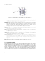
The CRAB rover is an autonomous robot of the Autonomous Systems Lab (ASL1 ) at
the Federal Institute of Technology Zurich (ETHZ). The CRAB is a 6 wheeled robot
based on two parallel boogies on each side as shown in figure 2.1. This buildup lets the
robot adapt to the ground which improves its terrainabliity. Also is he able to drive
over obstacles. More detailed informations about the chassis can be found in [4].
Figure 2.1.: Chassis of the CRAB in different positions adapted from [4]
In order to control the CRAB, the angle ηv and speed ωv of a virtual wheel have to
be set. This virtual wheel is located in the front of the robot as shown in figure 2.2.
When the speed and the angle for this wheel are set, the speeds and angles for all the
real wheels can be calculated. The speed of the virtual wheel is called virtual speed
and its angle virtual angle. The CRAB rover operates at low speeds, that means its
maximum allowed operating speed is 15 cm/s.
The software of the rover consists of several modules. Each module is able to send and
receive messages. This is done using Carmen IPC (Inter- Process Communication). A
survey on IPC is found in [6]. The modules can be started independently. The messages
are not sent to a module, they are sent to Central. If a module wants to receive
messages, it has to subscribe to them. There are different modes how to subscribe to
a message, a module can for example subscribe to all messages or just the latest one.
Normally, we just listen to the latest message in order not to introduce too much delay.
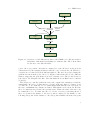
Figure 2.3 shows the different modules and how they are connected. As shown in the
image, several modules act as sender and receiver. The modules used in this work are
the following:
Rover Controller The controller accesses the motors of the wheels. It listens to the
1
http://www.asl.ethz.ch/
3
2. System overview
Figure 2.2.: Virtual wheel of the CRAB rover adapted from [5].
navigation messages which tell the desired virtual speed and virtual angle and
calculates the required speeds of the single wheels.
Navigation The navigation module calculates the needed virtual speed and virtual
angle and sends them to Central. It listens to several modules as the odometry
and the joystick module. This module was modified in order to handle obstacle
messages. Subsection 2.1.2 describes this module more in detail.
Odometry The robot odometry module measures the distance that the rover covered
and sends the actual position to Central.
IMU The Inertial Measurement Unit submits the orientation of the robot that means
the Euler angles to Central.
Joystick The joystick can be used to control the robot. The usage of the joystick is
enabled if the navigation mode is set to manual.
Obstacle Detection The obstacle detection module was developed during this project
and is newly integrated on the CRAB rover. It sends an obstacle map to Central,
which then in used in the navigation module. Detailed informations are shown in
chapter 3.
Estar The Estar module is a path planner which calculates the best trace.
2.1.2. Navigation module
The navigation module is where the obstacle informations are handled. The module
has three different modes, the manual mode, the trajectory and the goto mode. The
obstacle detection just works in the trajectory mode. Informations about the terrain
and the obstacles are saved into a grid. The grid building process is discussed in
chapter 4. Afterwards, the grid is sent to the Estar module. Estar is a path planer
based on weighted region approach [1]. A navigation function is computed from the
4
2.1. CRAB rover
IMU
Roll angle
Odometry
Joystick
Obstacle Detection
Virtual speed, Obstacle and
freespace
virtual angle
positions
Actual position
Trace
Estar
Navigation
Smoothed grid
Virtual speed,
virtual angle
Rover Controller
Speed and angle
of every wheel
Actuators
Figure 2.3.: Overview over the different modules of the CRAB rover. The arrows show
what kind of information is submitted to what module. The bold modules
are the new or modified modules.
goal to the rover position. Its value is computed for each cell based on the previous
cells traversed by the navigation function and the cost to traverse the cell. Therefore,
obstacles are accounted as well as different surfaces. The trace is produced using the
gradient descent from the goal to the robot. Figure 2.4 shows the trace for two different
surfaces, supposing the gray surface is worse for driving on it. The produced trace is
sent back to the navigation module. More informations about Estar can be found in
[7] and [8].
The trajectory controller verifies the trace and computes the virtual speed and the
virtual angle. In order to do that, first a good point on the trace has to be found to focus
on. Since we do not want the robot to make sharp turns when he is not precisely on
the trace, a minimum trace distance is defined. This distance is about 50 cm. Because
the robot may have moved since the grid was sent to Estar, the start of the trace can
lie behind the robot. To make sure the robot focus on a trace point lying ahead of
the robot position, the distance to the trace point is compared to the distance to the
following tracepoint. If the distance to the tracepoint is smaller, then the tracepoint
5
2. System overview
Figure 2.4.: Trace produced by Estar for two different surfaces adapted from [5].
lies in front of the robot. Otherwise we follow the trace until this criterion is achieved
and we have a minimum distance of 50 cm. Finding this point, the virtual speed and
the virtual angle is calculated and sent to the rover controller. The controller calculates
the speed and angle of each wheel and actuates them.
2.2. Stereo camera
2.2.1. General informations
As already said in the introduction, using stereo cameras allows creating 3D images. In
the left images features are detected which then are searched in the right image (or vice
versa). Because the two cameras are not located on the same place but with an offset,
the corresponding features do not lie on the same pixel of the image. The distance
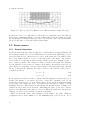
between the two viewpoints is called baseline. Figure 2.5 shows a simplified setup of
stereo camera geometry. The baseline is called b, f is the focal length. The disparity
d is the difference between the two features on the image. It is indicated in 1/16 of a
pixel. Therefore, a disparity of 32 represents a distance of 2 pixels in the image. Having
the two points and the disparity, the range r related to the cameras position can be
computed as follows:
d = dr − dl
(2.1)
r = b · f /d
(2.2)
From equations 2.1 and 2.2 it can be computed that the disparity d is inversely proportional to the distance r of a feature. In order to reduce the computing costs, one can
specify the search area for a corresponding feature. A big search area allows tracking
closer points, but it makes the stereo processing slower and the probability of wrong
matchings increases. This variable is called ndisp and its unit is pixel. If ndisp is for
example 48, the search area is 48 pixels. This limits the range of the stereo camera,
features closer than this point cannot be detected. When the features are far away, the
disparity becomes very low and the resolution downgrades.
Figure 2.6 shows the value of the disparity corresponding to the range. With the
configuration used on the CRAB rover, the minimum range is about 1.2 m. In or-
6
2.2. Stereo camera
Figure 2.5.: Buildup of a stereo camera.
Figure 2.6.: Disparity function with b = 9 cm, f = 6 mm. Low resolution means the
disparity difference is lower than 1/16 pixel per 10 cm range.
der to calculate the distance from the rover, the camera coordinate system has to be
transformed to a robot coordinate system. As shown in figure 2.7, the camera and the
robot coordinate system have the same x-axis. The transformation is done by rotating
around this axis by an angle θ, which depends on how the camera is mounted.
7
2. System overview

 
 
xr
1
0
0
 yr  = 0 cos(θ) sin(θ) · 
zr
0 −sin(θ) cos(θ)

 
 
xc
1
0
0
 yc  = 0 cos(θ) −sin(θ) · 
zc
0 sin(θ) cos(θ)

xc
yc 
zc

xr
yr 
zr
(2.3)
(2.4)
Figure 2.7.: Camera coordinate system compared to robot coordinate system.
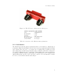
2.2.2. Videre Design Stereo Camera
The camera used in this project is a STH-MDCS2-C produced by Videre Design. Figure
2.8 shows how the camera looks like. Its baseline is 9 cm while the focal length of the
lenses is 6 mm. The 6 mm lens has a horizontal field of view (FOV) of 58.1 degree and
a vertical FOV of 45.2 degree. As the lenses are not fixed, it can simply be replaced
by another lens in order to change the FOV. The image resolution is up to 1280 x 960
pixels, but in order to have a higher frame rate we used images of 640 x 480 pixels. This
allows having frame rates of up to 30 Hz instead of 7.5 Hz using the high resolution
images. Therefore, the brightness of the images adapts faster to the environment. More
information on the camera can be found in the manual[9]. Table 2.1 shows the most
important camera properties and settings used for this work. All the camera settings
are saved in a file called vdisp.cfg. An actual version of this file can be found in the
appendix. It also includes the filter settings. The camera is mounted in front of the
CRAB at a height h of 70 cm.
8
2.2. Stereo camera
Figure 2.8.: The SVS stereo camera used for this project
Camera properties and settings
Type:
STH-MDCS2-C
Focal length:
6 mm
Baseline:
9 cm
Resolution:
640 x 480 pixels
Horizontal FOV:
58.1 degree
Vertical FOV:
45.2 degree
Table 2.1.: Overview of the different camera parameters
2.2.3. SVS Software
The Small Vision Systems (SVS) is an implementation of the SRI Stereo Engine[10]. It
works under Windows and Linux. SVS provides several programs and functions which
can be included into the source code. It supports for example image acquisition, storing
and loading image streams, image filtering, camera calibration and 3D reconstruction.
A detailed documentation can be found in [9]. Using smallvcal the camera is calibrated
very quickly. With the main program smallv, the actual images can be visualized and
different filter methods can be tested. It is also possible to store streams and load them
in order to test the filters with the same images.
9
3. Obstacle detection using stereo images
3.1. Obstacle detection algorithm
In order to avoid obstacles, they first have to be detected. There exist several approaches based on different sensor types such as infrared sensor, sonar or stereo camera.
Christophe Chautems [11] has developed an obstacle detection algorithm using a stereo
camera. An overview on the properties of stereo images was given in section 2.2. The
goal of this work was to improve this algorithm and integrate it on the CRAB rover. In
the semester project two different approaches were introduced. The first one was the
object segmentation, the second one the floor detection. Because the disparity images
are not exact due to noise, the task of object segmentation is difficult and the second
approach was chosen. In order to detect the floor a v-disparity approach was implemented. The v-disparity image is created using the disparity image using the following
algorithm:
foreach ith column on disp do
foreach j th line on disp do
if disp(i,j) > 0 then
vdisp(disp(i,j),j) ++
end
end
end
Algorithm 1: V-disparity, disp refers to the disparity image, vdisp to the v-disparity
image.
A property of the v-disparity image is that the floor is represented as a line if there is
no roll. Finding the floor, a minimum obstacle height can be set and everything that is
above this minimum height is marked to be an obstacle. Figure 3.1 shows the different
steps of this algorithm, the bold boxes are the new ones. First some words about the
original blocks:
Image source Input: Output: stereo
Description: The stereo image (stereo) is acquired and stored into memory. The
disparity is computed.
Disparity source Input: stereo
Output: disp
11
3. Obstacle detection using stereo images
Image Source
Only for display
Disparity
Roll Detection
Rotate Disparity
Vdisparity
Floor Detection
Show Line
Limit Obstacle
Show Line
Show Obstacle
Floor Map
Obstacle Map
IPC
Send Map
Navigation Module
Figure 3.1.: Obstacle detection algorithm. The new blocks are the bold ones, the other
blocks are obtained from the semester thesis. Some of them have changed
slightly. The blocks that are only for display can be removed without any
influence on the obstacle detection.
Description: The disparity (disp) was already computed in the image source block,
it just has to be copied and stored into the memory.
V-disparity Input: disp
Output: vdisp
Description: The v-disparity (vdisp) is calculated using the disparity image as
shown in algorithm 1.
Floor detection Input: vdisp
Output: floor
Description: Using a RANSAC approach the floor line (floor) is searched in the
v-disparity image.
Limit obstacles Input: floor
Output: limobs
Description: Giving an offset to the floor line, another line is generated that
describes the minimum obstacle height (limobs). Every point in the v-disparity
image lying above this line is an obstacle.
Obstacle map Input: disp, limobs
Output: map
12
3.2. Improvements
Description: The obstacles are searched in the disparity image and then transformed to the robot coordinate system. The obstacle coordinates are used to update an obstacle map (map) which holds the information about how many obstacle
pixels were detected in which cell.
Show line Input: floor/limobs, vdisp
Output: lfloor/lobs
Description: The floor line and the obstacle line respectively are plotted into the
v-disparity image. This block is just for visualisation.
Show obstacle Input: limobs, disp
Output: showobs
Description: Every point that is above the obstacle line remains in the new disparity image (showobs), the other ones are removed. Therefore just the obstacles
remain in the image.
This algorithm works fine if there is enough texture and no roll. Otherwise it fails.
If the obstacle detection does not work properly, it is difficult to generate accurate
obstacle prediction grids although several maps are used to generate them. Therefore
some improvements were made in order to make the obstacle detection more robust.
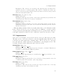
3.2. Improvements
As it can be seen in figure 3.1 four new blocks are developed. They have two tasks.
The first one is to detect the roll and to rotate the disparity image that the floor is
represented as a line again in the v-disparity image. The second one is to detect the
floor and send the obstacle and the floor information to the navigation block. The
following description shows what is the task of the new blocks:
Roll detection Input: disp
Output: roll image, roll angle
Description: Using the disparity image the roll angle is calculated. Furthermore
an image is created with the different gradients.
Rotate disparity Input: disp, roll angle
Output: rot disp
Description: The disparity image is rotated by the roll angle around the zc axis.
Floor map Input: vdisp, floor
Output: fmap
Description: Every point that lies close to the floor is transformed to the robot
coordinate system and stored into a floor map (fmap).
Send map Input: map, fmap
Output: sendmap
Description: The obstacle map and the floor map are fused into a new map
(sendmap) and sent to the navigation module.
13
3. Obstacle detection using stereo images
Additionaly some changes in the original blocks were made, such as, for example,
to be able to store and load image streams. This allows testing different algorithms
offline and compare them. The next subsections will describe the new blocks and
the modifications more in detail. More information on the original obstacle detection
blocks can be found in [11]. One change that had to be done for all blocks that use the
disparity image was that they now use the rotated disparity image. This concerns the
v-disparity, obstacle map and show obstacle block.
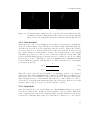
3.2.1. Image source
In order to make tests and to compare example different map building techniques, there
are now two different modes, an offline and an online mode as shown in figure 3.2. The
online mode works as the old one, but with additional possible adjustments. The image
streams can be saved as well as the time of acquisition. This allows reproducing a scene.
The offline mode loads an image stream and opens the image pairs in the timesteps
they were taken. Additionally to opening the images, position messages can be sent.
This simplifies testing a lot and allows comparing different settings for the camera
and for the map building. Figure 3.3(a) shows an example image, which was acquired
during a test and is now used to discuss the other blocks. The corresponding disparity
image is found in figure 3.3(b). The images were not taken at exactly the same time,
therefore there may be some differences the images as for example in the disparity and
the rotated disparity image.
Store image stream
Store position messages
Image Source
Online
Navigation
Module
Memory
Disparity
Image Source
Offline
Load image stream
and position messages
Send position
messages
Figure 3.2.: In the online mode the image streams can be saved into files, in the offline
mode they can be loaded. In both modes the stereo image pair is used to
calculate the disparity and then, the standard procedure begins.
3.2.2. Roll Detection
A problem of the existing obstacle detection was that it was not able to detect the
floor properly when there was roll. Therefore, a roll detection algorithm has been
implemented. According to [12] roll can be detected regarding on the yc displacement
of horizontal sections as shown in figure 3.4(a). To do that, the lower part of the image
is split in several sections. Their size can be changed very easily. A height of 10 pixels
14
3.2. Improvements
(a) Image source
(b) Disparity source
Figure 3.3.: The left image and its corresponding disparity image.
has proved to work well during tests. Because the floor is mainly found in the middle of
the image, especially when there is roll or we are avoiding obstacles, not the entire line
is analyzed. Within these sections, for every non zero disparity pixel, the yc coordinate
is calculated. When there is no roll, the yc coordinate should be the same for all the
pixels. But if there is roll, the yc value increases or decreases linearly. The gradient is
found with a RANSAC (RANdom SAmple Consensus) approach. Two random points
are selected and the points lying within a limit of the line are counted. This is done
several times for each section. In each section the line with the most close points is
chosen to be the best one. If there is a minimum number of points close to the line, the
gradient is stored, otherwise it is discarded and the section has no influence on the roll
detection anymore. Then, the gradients of all section are compared to each another.
The gradient with the most gradients from other sections being close to it is selected to
represent the actual roll. The gradients of the lower image sections count more because
we are mainly interested in the floor close to the robot. This approach works fine when
the disparity can be well detected and when there are few obstacles. If it does not work,
for example due to few textures or to many obstacles, another approach is chosen. If
there are not enough similar gradients or not enough points on these lines, the IMU
information is used to define the roll. The IMU has the advantage that it does not
depend on the disparity image, but it can just tell the difference between the robot
coordinate system and the world coordinate system. If the floor has roll itself, it is not
recognized. For the disparity image shown in figure 3.4(a) the roll lines look like figure
3.4(b). The roll angle is only set to a non zero value if a certain minimum value is
trespassed.
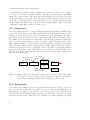
3.2.3. Rotate disparity
With the roll angle computed in the previous block, the disparity image is rotated
around its center that means around the zc axis. Figure 3.5 shows how the disparity
looks like after removing outliers and rotating. Since we rotate around the center, some
15
3. Obstacle detection using stereo images
(a) Image sections
(b) Roll detection
Figure 3.4.: Roll detection: The disparity image is divided into different sections (left
image). For each of this sections the gradient of the yc coordinate is found
(right). The best gradient is marked red.
of the informations in the edges may get lost.
Figure 3.5.: Rotate disparity: The disparity image is rotated by the angle submitted
by the roll detection.
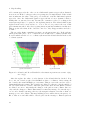
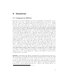
When the disparity is rotated, the floor is represented as a line again in the v-disparity
image. Figure 3.6 shows two different images, one where the disparity image has been
rotated, one where the disparity image was not changed. The green lines are the floor
lines, the red lines the minimum obstacle height. As you can see, in the right image the
floor is extended and not represented as a line. Therefore, the floor was not detected
properly.
16
3.2. Improvements
(a) With roll detection
(b) Without roll detection
Figure 3.6.: V-disparity image with plotted floor (green) and obstacle limit (red). The
left image shows the v-disparity where the roll is detected and the disparity
image rotated, the right image shows the v-disparity disregarding the roll.
3.2.4. Floor detection
When there is no roll or it is eliminated, the ground is represented as a straight line
as the green line in figure 3.6(a). This line is determined using a RANSAC approach.
As in the roll detection block, two randomly points are chosen to define a line. If there
are more points close to this line than in the former tries, this line is saved as best
line. This continues a certain number of times. As an improvement to the original
algorithm, the points close to the robot are counted more than the ones far away. This
reduces effects like fitting the line trough far obstacles or, if there are two slopes, taking
the farer slope as floor. Furthermore, there is a minimum and a maximum gradient
between which the gradient of the line has to lie. These gradients can be found using
some trigonometry [13]:
h
gmin =
(3.1)
16 ∗ b ∗ cos(θmin )
gmax =
h
16 ∗ b ∗ cos(θmax )
(3.2)
When the best floor line is found, the number of points lying on the floor is compared
with a previously defined minimum number. If it is lower than this, for example due to
bad texture, the rover is assumed to stay evenly on the floor, ignoring roll and pitch.
This can happen in indoor environments, where the stereo camera may not be able to
detect the floor. In such environments this approach often is true. If there are enough
features found on the floor, the floor is used to find the obstacles.
3.2.5. Map blocks
After detecting the floor, an obstacle limit is set. The minimum height for an obstacle
is set in the vdisp.cfg file. A plane is defined parallel to the floor plane. This plane
is also represented as a line in the v-disparity image (red line in figure 3.6(b)). Every
point in the v-disparity image lying above this line is considered to be an obstacle.
17
3. Obstacle detection using stereo images
This steps remained the same. Using the information about the detected roll and the
floor, the obstacles are transformed into the rover coordinate system. Newly one has
to consider the roll for the backtransformation. The obstacles are put into an obstacle
map. For any detected point the value of its corresponding map pixel is increased by
one. The higher the values of the obstacle map are, the more authentic is the obstacle.
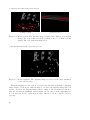
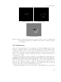
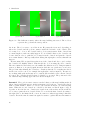
Figure 3.7(a) shows an obstacle map.
Newly the same thing is done with the floor. Any pixel close to the floor line is
believed to be part of the floor. It is transformed into the rover coordinate system and
a map is created. An example is shown in figure 3.7(b). These two maps are combined
into another map using algorithm 2. Setting a minimum value for the obstacle and
for i = 0 to MapSizeX do
for j = 0 to MapSizeY do
sendmap(i,j) = 0 if fmap(i,j) > minFloor then
sendmap(i,j) = -1
end
if map(i,j) > minObst then
sendmap(i,j) = 1
end
end
end
Algorithm 2: Combine the obstacle map (map) and the floor map (fmap)
the floor map allows filtering out simple outliers, where just few features are matched
wrongly. If a cell is obstacle and floor at the same time, its status is set to obstacle.
Because every obstacle that lies directly on the floor has some points that are very close
to the floor and therefore are regarded as floor.
The combined map, more precisely the obstacles and the floor are saved into an
array and sent to the navigation block as obstacle prediction message, where they are
proceeded further. Figure 3.7 shows the three different maps for the situation given in
figure 3.3(a).
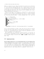
3.3. Implementation
The algorithm is written in C++. It uses IPL (Intel Image Processing Library). The
framework was implemented by Cédric Pradalier and needs the usage of Dynamic Data
eXchange (DXX) [14]. Using the function sdlprobe, the different images of the obstacle
detection algorithm can be visualized. Using a configuration file the different parameters of the obstacle detection algorithm can be changed. This file is called vdisp.cfg,
an actual version can be found in the appendix or on the supplemental CD. The configuration file allows to make changes without recompiling the obstacle detection.
18
3.4. Performance
(a) Obstacle map
(b) Floor map
(c) Combined map
Figure 3.7.: The obstacle map and the floor map are used to create a combined map
holding all the information. Cells where the value is not high enough are
not considered.
3.4. Performance
The new blocks make the stereo processing more robust and slightly slower. But a
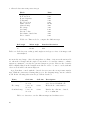
frequency of 5 Hz can easily be reached, what is sufficient for the map building. Table
3.1 shows the time needed for each block. In average 109 ms are needed for one cycle.
That would be a frequency of about 10 Hz. Because the robot is moving at low speeds
and we do not want the overload the navigation module, we run the obstacle detection
at a frequency of 5 Hz.
The roll detection has been tested on flat floor, the results can be found in table 3.2.
As assumed the quality of the roll detection decreases the higher the roll is. One cause
is that the floor on one side comes closer until it is too close to be detected. Therefore
there are less features to find the roll angle. If there is an obstacle right in front of
the robot, the roll detection may be corrupted. But when there is an obstacle, the
gradients or the different sections normally are not about the same, therefore the roll
detection will be ignored and the IMU information is used.
Tests have shown that the stereo camera used on the CRAB is more precise than
19
3. Obstacle detection using stereo images
Block
Image acquisition
Roll detection
Rotate disparity
V-disparity
Floor detection
Limit obstacle
Obstacle map
Floor map
Send map
Show floor line
Show limit obstacle line
Show obstacle
Time
50 ms
8 ms
4 ms
5 ms
8 ms
10 ms
4 ms
3 ms
1 ms
4 ms
4 ms
8 ms
Table 3.1.: Time needed to compute the different steps
Roll angle
0
15
Mean angle
-0.067
14.989
Standard deviation
0.317
0.94
Table 3.2.: Roll detection on flat ground, angles are in degrees. A set of 50 images each
was analyzed.
10 cm in the used range. Since the maps have a cellsize of 10 cm as shown in table
3.3, when the roll angle and the angle θ between the robot and the camera coordinate
system are estimated correctly, the generated maps are precise. However the obstacles
will be slightly dilated in the navigation module in order to be sure to avoid such and
other errors as will be shown in chapter 4.
A problem that occured with the obstacle detection were the wrong feature matchings. With the camera used during this project, the disparity image was not reliable
at all. In the following subsection the problem is described.
Name
Obstacle map
Floor map
Combined map
Grid size
5.1 x 5 m
51 x 50
5.1 x 5 m
51 x 50
5.1 x 5 m
51 x 50
Cell size
0.1 m
0.1 m
0.1 m
Description
Saves how many obstacle pixels
were detected in which cell
Holds the floor information
Divides the cells into obstacle,
floor or unknown
Table 3.3.: Overview over the different maps used in this section
20
3.4. Performance
3.4.1. Disparity problem
The disparity problem occured in all kind of environments. There were tries to characterize this wrong feature matchings. The errors mainly occur in structured environments, indoor as well as outdoor. They occur when there are bricks, metallic or just
bright surfaces, but they also occur in real outdoor environments, for example when
there are leaves or grass. Another characteristic is that if there is for example a horizontal object, depending on whether you turn the camera to the left or to the right, the
object is detected to be very close or far away. Therefore it was not possible to filter
the disparity image without removing many true matchings. The problem is that these
wrong matchings do not just appear and disappear, the computer is sure the obstacles
were there. Filter methods included in svs software as uniqueness or confidential filter
did not lead to success. Also new calibration was useless.
There were several approaches in order to remove this kind of errors. The first
one was the filtering using the integrated filter methods as uniqueness or confidential
filter, but this did not work. We detected that the wrong matchings often occured at
the maximum disparity value, that means the features were thought to be very close.
Therefore all close features are deleted. This removes also some true information and
increases the minimum range to detect a feature, but the disparity errors could be
reduced by about 70 percent. We also tried to calculate the disparity on our own using
opencv, but this slowed down the entire process and the disparity images (the true
matchings) were less precise.
Another idea to remove errors that appear frequently was to analyze the obstacle
and floor positions. If for example we have floor on the same place as the obstacle is
located and also in the cell behind, one could say there is no obstacle. This is acceptable
approach for all kind of obstacles that rise from the ground, but for trees for example
this would not work. This limits the field of application. Because the stereo camera
did not deliver very precise disparity images and therefore just small parts of the floor
were detected, this approach was not used during the tests.
The disparity problem has not been solved yet. Although a map building algorithm
is used that removes random errors, the disparity errors that occur very frequently
are transfered to the obstacle prediction grid and the robot tries to avoid these wrong
obstacles.
The obstacle detection algorithm can easily be adapted to other Videre Design stereo
cameras. For the final test on the CRAB rover, another stereo camera was used. With
the new camera reliable maps were produced and the tests succeeded. Because the
new camera computes the disparity on the camera hardware, the offline mode does not
deliver the same results.
21
4. Map handling
As important as the obstacle detection is the map handling. The map handling is about
how the maps generated in the obstacle detection module are used in the navigation
module. The handling starts when an obstacle message is received and ends when the
Estar message is sent.
There exist many different approaches, very simple ones that just consider the actual
image and more sophisticated ones that also consider the previous images. If you
want to consider also the previous images of a moving robot, you have to know its
displacement. In this work two variables are used to describe the dynamic behavior
of a map building algorithm, the time to show an obstacle (TSO) and the time to
show a hole (TSH). The goal is to keep these times low as well as make accurate maps.
Unfortunately these wishes are conflictive. Before introducing the CRAB algorithm, the
next subsection shows three different popular approaches, a probabilistic, a constant
add and a differential equation approach. To be consistent, i means the position of
the obstacle, v(i) the value of the sensor data (1 for obstacle, -1 for freespace) at the
position i and grid(i) corresponds to the value of the obstacle grid. The map building is
done in several steps, where t means the actual step and t−1 the last one. The obstacle
detection operates at a frequency of 5 Hz, so does the map handling. Therefore one
step corresponds to 0.2 seconds.
4.1. Different approaches
4.1.1. Add constant
One of the simplest map building approach is just adding or subtracting a constant
value depending on what the input value is as shown in algorithm 3. We call this the
AC (Add Constant) approach [15]. The TSO and TSH only depend on the factor K.
Figure 4.1 shows the behavior of this algorithm for different K’s, assuming that cell
holds an obstacle if its value is above 0.9 (black dots). The high red dots mean there is
an obstacle as input, the low ones there is freespace. This algorithm can be improved
by taking different factors for increasing and decreasing the grid value. Because it is in
our case more important to see the obstacles quickly than to detect a hole, the K for
increasing is chosen to be higher. This algorithm has been tested using Webots and on
the CRAB rover. A value of 0.1 for the increasing K and 0.05 for the decreasing one
has proven to be a good choice. Assuming we have a frequency of 5 Hz, the TSO is at
maximum 1.8 s and two wrong guesses are not enough to remove an obstacle. But the
disadvantage of this is that it takes 20 steps to remove an obstacle entirely. If we have
much noise, where every third time an obstacle may occur, this approach leads into
23
4. Map handling
if v(i) == obst then
grid(i) = grid(i) + K;
if grid(i) > 1 then
grid(i) = 1;
end
end
if (v(i) == f ree) then
grid(i) = grid(i) − K;
if grid(i) < 0 then
grid(i) = 0;
end
end
Algorithm 3: Add constant.
Figure 4.1.: Add constant algorithm for different K’s. Red dots: Input signal. Red line,
the algorithm implemented on the CRAB rover
troubles. Because then, if an obstacle is set once, it is not removed anymore. When
the K is too high, errors in the obstacle map may have a big influence on the obstacle
grid, e.g. obstacles are removed after one wrong guess. In red you can see the approach
implemented on the CRAB rover. Additionally a forgetting function is implemented,
that removes an obstacle after a certain number of steps if there is no input.
24
4.1. Different approaches
4.1.2. Probabilistic approach
The probabilistic approach is very established approach to build occupancy grids. It
assumes that each cell can only be in two states, occupied or empty. The cells are
initialized at 0.5, what means the actual state is not known. If the value is close to one,
this cell is believed to be occupied, if the value tends towards zero, the cell is empty. A
sensor collects the new values, which are used to update the grid. One possible update
rule is the Bayes rule [16]. This update rule looks as follows:
grid(i) =
p(i, obst) · grid(i)
p(i, obst) · grid(i) + (1 − p(i, obst)) · (1 − grid(i))
(4.1)
In order to calculate p(i, obst) a sensor model has to be developed. A possible approach
for a for a sonar sensor is given in [16]. Due to analyze the behavior of this approach
a very simple model has been implemented.
(
c,
v(i, t) > 0
p(i, obst) =
(4.2)
1 − c, v(i, t) < 0
0.5 < c < 1
(4.3)
The value of p(i, obst) just depends on the input and a constant c that defines the
probility the sensor information is correct. Figure 4.2 shows the behavior for different
inputs for different p(i, obst). One of the problems using this kind of approaches is that
if the sensor values stay for example -1 for a long time, if an obstacle appears it is not
detected fast enough since all the former freespace messages have to be compensated.
Because of likely odometry errors especially when driving offroad, that kind of behavior
can lead to troubles. If the robot saves an empty cell and suddenly, due to odometry
errors there is an obstacle, it can take too long to change the cell status, the TSO can
become very high. Due to this behavior, this approach was not investigated further
and no sensor model was developed.
4.1.3. Differential equation approach
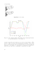
Another approach investigated by Canas [17] is the differential equation approach.
Using the old grid, the sensor data, a saturation, a sequence and a speed factor the
new grid value is calculated.
grid(i, t) = grid(i, t − 1) + v(i, t) · sat(i, t) · seq(i, t) · speed
(
|1 − grid(i, t)| ,
v(i) > 0
sat(t) =
|−1 − grid(i, t)| , v(i) < 0
(4.4)
(4.5)
The sequence factor can be between 0 and 1. If the previous sensor data looks the same,
it is increased. If they do not, it is decreased. This helps to minimize the influence of
outliers. The dynamic behavior mainly depends on the speed factor, in some cases also
25
4. Map handling
Figure 4.2.: Probabilistic approach for different sensor probability values. Red dots:
Input signal.
the sequence factor may have a big influence. One improvement that was made while
installing it on the CRAB is that there is a forgetting factor for each step.
grid(i) = 0.99 ∗ grid(i)
(4.6)
Using these equations, the grid value lies between -1 for freespace and 1 for obstacle.
In order to integrate different algorithms to the navigation module, they have to be
consistent. The value of this grid can easily be transformed into a value between 0
(freespace) and 1 (obstacle) using the following equation:
gridneu (i) = (grid(i) + 1)/2
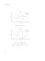
(4.7)
Figure 4.3 shows the behavior for different speeds. For a speed of 0.5 the TSO and the
TSH is 0.6 seconds. If we do not have any new information about the grid, an obstacle
is removed after 4 seconds. This makes sense, because due to odometry errors, the
obstacle may now be in another cell. Using a good algorithm to calculate the factor seq
this behavior can be improved. On the CRAB a very simple approach is taken. If the
cell value is above 0.9 and a freespace occurs, then the seq factor is chosen to be 0.3.
This allows keeping the cell status longer. The same is done when the value is below
0.1, but then an obstacle input reduces the seq value. In all other cases, this value is
1. The method implemented on the CRAB is the red function shown in figure 4.3. It
is slower than the other two functions, but it is less prone to errors.
26
4.2. Map building on the CRAB rover
Figure 4.3.: Differential equation algorithm for different speeds. Red line: The method
implemented on the CRAB rover.
4.1.4. Comparison
Two approaches were implemented and tested in Webots and on the CRAB rover.
These were the differential equation approach and the add constant approach. The
problem with the probabilistic approach is, that it may take very long until an obstacle
is removed. If we have 100 messages that say it is an obstacle, 100 freespace inputs are
needed to remove it entirely. Since the CRAB is designed to drive on offroad terrain,
the odometry may not be very reliable. Therefore, an obstacle has to be placed or
removed fast if it is needed. The differential equation approach has the most tuning
parameters, the time to place an obstacle and the number of freespace messages needed
to remove it again can be set easily using a certain sequence factor. So, mainly the
differential equation approach was used during tests, the add constant approach was
just used for comparing reasons.
4.2. Map building on the CRAB rover
Now to how the map building works on the CRAB rover. Table 4.1 gives an overview
over the different grids used in this section. As seen in the last chapter, a map is
created using the information from the stereo camera. The obstacles and the floor
are sent to the navigation module using Carmen IPC. This message is called obstacle prediction message and contains how many obstacles/freespace were found, their
27
4. Map handling
Name
RoverViewGrid
Grid size
5.1 x 3.8 m
51 x 38
Cell size
0.1 m
ObstacleGrid
12 x 12 m
120 x 120
0.084 m
GridRtile
21.5 x 21.5 m
256 x 256
0.084 m
GridSmoothed
21.5 x 21.5 m
256 x 236
0.084 m
Description
The map from the obstacle detection algorithm saved in this
grid and modified
This grid contains the obstacle
probability and is updated using the RoverViewGrid
If the probability is high enough
it is saved in this grid. There,
the data of several sensors can
be fused; it for example may
content terrain information
Is a smoothed version of GridRtile. This grid is sent to Estar
Table 4.1.: Overview over the different grids used in this section
position and a value. A value of -1 means it is freespace, a value of 1 means there is an
obstacle. In order to get more information out of the created map, the obstacles are
saved in a grid referred to as RoverViewGrid, which is reinitialized for each new image.
The idea of this grid is to save all the knowledge and do some interpretations. Its grid
size is the same as the one of the combined map. The obstacles and the freespace are
saved into that grid. As an example we take the combined map from figure 3.7(c).
Since the stereo camera and especially the robot odometry are not precise, an uncertainty is added. Based on the horizontal and vertical uncertainty the obstacles are
dilated, the freespace remains the same, if it is not overwritten by a dilated obstacle.
Figure 4.4 shows an example. An overview over all the functions used for the map
handling is found in table 4.2.
Using trigonometry, the minimum and maximum angle of an obstacle cell is calculated. The values are saved in an array for every obstacle. Because the field of view
is limited, it does not make sense to transmit information about the entire map to the
next function. Therefore outside the field of view we save a dump result, what makes
it easy for the next function to recognize what is the important information. Because
the stereo camera is not able to recognize anything closer than 1.2 m, we also store a
dump result in there respectively the grid is shortened that it does not contain the first
1.2 m. Figure 4.5 shows the area that is proceeded further.
Starting at the left bottom of the stereo view area the cells are analyzed. If the cell
already has a status, freespace or obstacle, the status is kept. Otherwise we check if the
cell is behind an obstacle, then its status is set to occluded. When this is not the case,
its status is set to freespace. How this works in detail can be seen in algorithm 4. The
RoverViewGrid is divided into four sections, freespace (green), occluded space (blue),
obstacles (red) and a dump result (gray) to mark areas where the stereo camera cannot
detect anything as shown in figure 4.6. In the algorithm obst stands for obstacle, occ
28
4.2. Map building on the CRAB rover
Name
ModifyObstacleMap
RoverViewToObstacleGridAC
RoverViewToObstacleGridDEq
ObstacleUpdateMap
ObstacleGridOffset
ProcessGrid
Description
Divides the obstacle map into obstacles,
freespace and occluded space and saves this
into the RoverViewGrid
Transfers the RoverViewGrid to the ObstacleGrid using the AC algorithm, needs the yaw
angle to do that
Transfers the RoverViewGrid to the ObstacleGrid using the differential equation approach,
it also needs the yaw angle
Saves the detected obstacles into GridRtile,
using the actual position of the robot
Moves the ObstacleGrid by a transmitted offset when the rover moves
Dilates the obstacles, smoothes the grid, dilates the obstacles once more
Table 4.2.: The functions used for map building
Figure 4.4.: The obstacles are dilated by a small factor. Although the cells status is
floor, it is overwritten by the dilation. The dilated pixels are marked red.
for occluded and free for freespace. The dump result is used to initialize the grid.
The next step is to include the RoverViewGrid into the ObstacleGrid. This grid
holds the information about the probability of a cell being an obstacle. Its size is 12
m x 12 m and the robot is located in the middle. This is in contrast to the other grids
as the Estar and the Rtile grid where the grid does not move and the center is located
29
4. Map handling
Input: RoverV iewGrid ← Grid with dilated obstacles and already detected
freespace
Output: RoverV iewGrid ← Grid with obstacle, freespace and occluded space
information
foreach ith column in FOV in RoverViewGrid do
foreach j th line in FOV in RoverViewGrid do
if RoverV iewGrid[i][j] == obst then
if i < Of f set X & RoverV iewGrid[i − 1][j]! = obst then
RoverV iewGrid[i − 1][j] = occ;
end
phi min[index] = arctan(i − Of f set X)/j);
phi max[index] = arctan(i − (Of f set X + 1))/j);
index + +;
end
else
foreach k th element of phi do
if arctan((i − (Of f set X + 1))/j) <= phi max[k] &
arctan((i − Of f set X)/j) >= phi max[k] then
RoverV iewGrid[i][j] = occ;
break;
end
end
RoverV iewGrid[i][j] = f ree;
end
end
end
Algorithm 4: Algorithm to detect occluded space
30
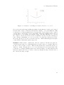
4.2. Map building on the CRAB rover
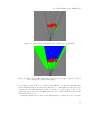
Figure 4.5.: Field of view (blue lines) and occluded space (black lines)
Figure 4.6.: The four sections of the map, obstacles (red), freespace (green), occluded
space (blue) and a dump result (gray)
at the start position of the robot. The moving with the robot has the advantage that
just needful information are saved and that the robot always knows where the close
obstacles are. Another advantage is that even if the robot moves close to the border
of the rtile grid respectively the Estar grid, the close obstacles still are saved in any
direction from the robot.
As already mentioned two modes were implemented to update the grid, one is the
31
4. Map handling
add constant approach, the other one is a differential equation approach as discussed
in section 4.1. In the both approaches a forgetting factor is implemented. If the actual
state is unknown, the value of the grid goes towards 0.5, as in the differential equation
approach. Since the differential equation approach has a better dynamic behavior,
mainly this one was used for tests. Because the orientation of the robot changes, the
actual yaw angle has to be passed to the updating function. The ObstacleGrid is just
updated in the field of view and not too close to the robot’s position, the rest of this
grid remains untouched. Also the forgetting function just has an influence in this area.
This stops the effect that, if the obstacles come close, they disappear what can lead to
a crash.
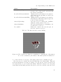
The two grids during a simulation scenario are shown in figure 4.7. Both grids are
taken at the same place, one to consider they are in different coordinate systems. The
RoverViewGrid is in the robot coordinate system and the ObstacleGrid is in the world
coordinate system.
(a) RoverViewGrid
(b) ObstacleGrid
Figure 4.7.: Obstacle and RoverViewGrid for the situation given in test scenario 3 (figure 5.1(c))
After the update the value of each element of the ObstacleGrid is checked. If it
above 0.9, an obstacle is placed in GridRtile at these coordinates. After setting all
the obstacles the usual GridRtile process starts. This process is also used in order to
distinguish different terrains. The obstacles are dilated, so that not only the middle of
the rover surrounds the obstacle. Then the grid is smoothed and the initial obstacles
are dilated once more. Afterwards the changes of the grid are sent to Estar. Since we
only send the changes to Estar, Estar must not miss any message. It can take up to
one second to handle a message, therefore the navigation must not send more than one
message per second to Estar. The map building however still works at a frequency of 5
Hz, so that we a can build reliable obstacle grid, but the message to Estar is just sent
32
4.2. Map building on the CRAB rover
one per second.
The differential equation approach is slightly slower than the constant add approach.
From the time the obstacle message is received until the Estar message is sent, the
constant add approach needs 40 ms while the differential equation approach needs 46
ms. But both algorithms are very fast and do not slow down the navigation module
unnecessary.
33
5. Simulation
5.1. Integration to Webots
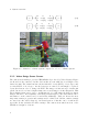
First test were performed with Webots1 . Webots is a simulation environment for robots.
Since there are no stereo cameras in Webots, 19 infrared sensors were used to emulate
the stereo camera. The infrared sensors are located in front of the robot, covering
the same field of view as the stereo camera would. From the sensor data, a map of
5.1 m x 5 m is created and sent to the navigation module. The size of the map is the
same as if it was generated in the obstacle detection algorithm, but it just includes
obstacles and no freespace. The simulation allows testing the map building algorithms
without using the CRAB and the stereo camera. First tests using just the actual map
have shown that it is very important to use some more advanced algorithms to build an
obstacle grid. Because using the stereo camera the features closer than 1.2 m cannot be
detected, the infrared sensors were programmed to have the same property. This leads
to the fact that the rover registers an obstacle, when it is far away, but when he gets
closer, the robot forgets that there was an obstacle and drives right into the obstacle.
Using the algorithms described in section 4 the obstacles are saved and they do not
disappear when the robot comes closer. The problem still occurs when the robot is
placed right in front of an obstacle, then he is not able to detect it. Also if it is located
few more than 1.2 m away. This is because the map building algorithm needs some
time to define an obstacle in the grid, the TSO. So, the user must not place the robot
close to an obstacle or another sensor has to be used for the area close to the rover.
Several scenarios were tested in order to learn the robot behavior when driving in an
environment with obstacles. Three scenarios are presented in order to describe some
properties of the map building. The scenarios are shown in figure 5.1. In Webots the
robot has no odometry errors, so it is possible to create very precise obstacle maps,
what is not the case on the CRAB rover. Therefore the difference between the two
updating rules is very small.
Scenario 1 The first scenario (figure 5.1(a)) includes one obstacle in front of the robot.
The goal was to see how fast an obstacle is detected and if the trace is smooth. Tests
have shown that depending on how the obstacle was placed, the robot was not able
to avoid it. Like discussed before, if the obstacle is too close, it cannot be detected.
Another problem was caused by the same characterics. With the infrared sensors, the
robot is just able to detect the front of an obstacle. This not only happens with infrared
sensors, if the obstacle is higher than the stereo camera, it also is just possible to see
1
http://www.cyberbotics.com/products/webots/
35
5. Simulation
(a) Scenario 1
(b) Scenario 2
(c) Scenario 3
Figure 5.1.: The different scenarios where the map building was tested. The red dots
represent the goal and the start position.
the front. The robot tries to avoid the front. He passes the front and, depending on
where the obstacle and the goal are, turns towards the back side of the obstacle. The
robot may be too close to the obstacle’s side to detect any features. If the obstacle has
a certain length a crash can easily happen. To avoid this behavior, the obstacles can
be smoothed in order to push the robot away from the obstacle and pass the obstacle
in a certain distance. But especially when driving through tight corridors, this still can
happen.
Because using Webots just delivers the front of the obstacle and due to grid overlays,
the obstacles are slightly dilated. This should also be done using the stereo camera.
The more infrared sensors there are, the smaller the dilation needed. Using 19 infrared
sensors, a dilation of one pixel (equals 10 cm) worked fine, two pixels were even better.
The problem when dilating the obstacles too much is, that the robots agility is reduced
and he is not able to move for example through tight corridors anymore. Because we
are working with grids and it may not be entirely sure in which of the cells an obstacle
is located, the obstacles should at least be dilated by one pixel. The positions for the
two different map building approaches are shown in figure 5.2.
Scenario 2 The goal of scenario 2 was to test the behavior of the map building methods
when obstacles suddenly appear. As shown in figure 5.1(b), the two obstacles are placed
with a certain distance. If the robot sees both obstacles, he has no problem avoiding
them. When the second obstacle is occluded by the first one like in figure 5.3(b), it
depends on how far the two obstacles are apart from each another and how fast the
robot can recognize the new obstacle. If the robot avoids the first obstacle, he turns to
the right. Due to the limited field of view, he cannot see what is appearing behind the
obstacle. From the time he turns left again, he starts to gather this new information.
36
5.1. Integration to Webots
Figure 5.2.: Scenario 1: Avoiding an obstacle. Goal at x = 5, y = 0.
Now, it depends on the map building algorithm, how far this new obstacle can be placed
from the first obstacle. Tests have shown that a distance of 1.2 m is sufficient. This
because the robot already turns left before he passed the obstacle, therefore the occluded
obstacle may be in the field of view. Depending on the map building method and on
how fast the robot is driving, the distance varies. The time until the robot detects
the occluded obstacle and receives a trace from Estar can vary. Because a message is
sent to Estar at maximum once per second, the robot may have already moved into
the wrong direction before he receives the new trace. This is what happened in figure
5.3(b) with the differential equation approach.
Scenario 3 This scenario combines the other two scenarios. We have the same two
obstacles as in scenario two, additionally there is a wall on the robot’s right. Therefore
he has to drive trough a corridor. This test has shown that obstacles should not be
dilated too much, otherwise the robot does not find any trace in between them. The
positions for both map building methods are shown in figure 5.4. Especially the last
turn was critical, since the robot has to turn very sharply he may touch the back of
the obstacle if it large enough.
37
5. Simulation
(a) Two independent obstacles
(b) Second obstacle partially occluded
Figure 5.3.: Scenario 2: Goal at x = 9, y = 0.
38
5.1. Integration to Webots
Figure 5.4.: Scenario 3: Driving through a corridor. Goal at x = 9, y = 0.
39
6. Integration on the CRAB rover
The stereo camera has been mounted on a camera rack in front of the robot at a height
of 0.7 m. Since there is another camera installed in front of the CRAB rover, it had
to be installed on the same rack, below the other camera. In order to test the obstacle
avoidance on the CRAB rover, several modules have to be installed and activated.
Additionally to the obstacle detection and navigation module are these the controller,
odometry, joystick and IMU module as well as the Estar module. Compared to Webots,
more modules are running at the same time. It is not possible to plot or save grids
during driving, otherwise the navigation module would become too slow. Because the
plotting can take more than one second, position messages could only be received every
second and the move message could just be sent once per second. Due to this, the
joystick can be used to plot and save the grids. First step is to disable the navigation
module in order not to receive any new information that could influence the grids.
Then, pressing the corresponding buttons, the grids can be plotted and saved. In the
end, the robot can be reactivated again using the joystick and he continues moving is
if there was no break. Table 6.1 shows the different commands.
Move message
vspeed = 0 cm/s
vspeed = 3 cm/s
vspeed = 6 cm/s
vspeed = x cm/s
Behavior
Stops the robot and the navigation module and activates the plotting mode
The actual ObstacleGrid and RoverViewGrid are plotted
The actual ObstacleGrid and RoverViewGrid are saved
into a file
If the command is neither 3 cm/s nor 6 cm/s, the navigation process is resumed
Table 6.1.: Usage of the joystick in the trajectory mode. Note that the plotting and
saving just works if the navigation module is stopped. Otherwise joystick
commands have no influence on the robot in the trajectory mode.
41
7. Test results on CRAB rover
7.1. Setup
Several things had to be adapted during the tests. Using the given stereo camera it
is not possible to make reliable obstacle avoidance as discussed in subsection 3.4.1.
The obstacles are avoided, but there seem to be obstacles where actually is free space.
Because the wrong obstacles often occur close to the robot, he turns in order to avoid
the obstacles and suddenly he is surrounded by imaginary obstacles. After some of these
errors were removed, there were some test runs that succeeded. But with increasing
run length, the probability that there are wrong disparity images that lead to wrong
obstacles increases. Therefore, the obstacle avoidance is not reliable at all. Reducing
the map building speed so that it takes longer to detect an obstacle does not lead to
succeed either, because this wrong matchings are not just an one time appearance,
some of them appear more often than the real obstacles. To cover these wrong features
does not make sense, because as soon as the robot turns, he sees other wrong features
that are not hidden. After several tries, we decided to take another stereo camera in
order to have a better disparity image. In contrast to the old camera, the disparity
is computed directly on the camera. Figure 7.1 shows an image and table 7.1 shows
some properties of the stereo camera. The minimum distance at which features can be
detected is slightly higher, it is about 1.5 m. Therefore the update ostacle grid function
has to be modified in order not to remove obstacles closer than this 1.5 m. As shown
in the appendix the configuration file changed slightly and another calibration file has
to be taken. All the files can be found on the supplemental CD.
Two scenarios were tested with the two stereo cameras. In order to compare the
results to the simulation results similiar scenarios were chosen. The first one was to
avoid a single obstacle as shown in figure 5.1(a) and the second one to avoid two
obstacles with a certain distance like in figure 5.1(b). In figure 7.2 you find an image of
Camera properties and settings
Type:
STOC15cm
Baseline:
15 cm
Focal length:
3.6 mm
Resolution:
640 x 480 pixels
Horizontal FOV:
56 degree
Vertical FOV:
44 degree
Table 7.1.: Overview of the different camera parameters
43
7. Test results on CRAB rover
Figure 7.1.: STOC stereo camera.
the second scenario we tested. The obstacles are positioned with a distance of about 2.2
m. The positions shown in the result section are obtained from the odometry module
and therefore not very precise.
Figure 7.2.: Scene overview during test run with two rows of obstacles.
7.2. Results
With the original stereo camera, some successful tests were made. The add constant
approach did not work properly due to the disparity errors and the noise, therefore
the differential equation approach was used for the tests. The first scenario with one
obstacle succeeded, but not very often. Because the entire obstacle detection process
takes quite long, the robot started to make strange movements as shown in figure 7.3.
44
7.2. Results
Analysing this behaviour led to the conclusion that the trace following does not work
Figure 7.3.: Scenario 1: Strange robot behaviour, position of the robot. The obstacle
(red) approximately shows where the real obstacle was located.
correctly. This problem was fixed by introducing new restrictions for the tracepoint to
follow as discussed in section 2.1.2. Afterwards, the trace looked smoother but there
still were corners because of the wrong feature matchings. Sometimes, they did not
influence the trace and sometimes they did. The second scenario was not completed
because in all the tests there appeared false obstacles and the robot did not know how
to continue.
Using the new stereo camera, the tests succeeded. Since the first scenario was no
problem at all, we focussed on the second one. Figure 7.2 shows the positions during
three different runs. The positions are obtained from the odometry module. The
obstacles are approximately marked in this figure. Figure 7.2 shows the temporary
goals for the two runs. As one can see the shape of the trace looks similar, but they
are not congruent.
The robot avoided the obstacles in all three runs and finally reached the goal. We
think the difference in the position and trace images is mainly due to odometry errors,
because in all three runs the robot had about the same distance to the obstacles. The
temporary goals image shows an offset sometimes. This is because we are working
with grids, if the robot moves a certain distance, there may occur an offset of one cell
when passing the obstacles to the rtile grid. Another interesting fact is, that until
the obstacles are recognized, the robot moves straight forward or even to the wrong
side. This can happen if the robot first recognizes the obstacles on one side, sends this
to Estar and afterwards detects the obstacles on the other side. At the moment he
recognizes all the obstacles, he starts turning in order to avoid them.
The high minimum range and the limited field of view are a serious problem when
using a stereo camera for obstacle detection. With the new stereo camera the same
problem occured as in webots. In one test run, the first obstacle was high and wide,
therefore the robot was not able to detect the back of the obstacle and had to be
stopped manually in order to avoid a crash.
45
7. Test results on CRAB rover
Figure 7.4.: The positions during two test runs.
Figure 7.5.: The temporary goals obtained from the actual traces.
7.3. Summary
The original stereo camera did not lead to success, the wrong matchings influenced the
robot’s behaviour too strongly. Taking another stereo camera the tests could be accomplished. One problem of this new camera was the increased minimum range to detect
46
7.3. Summary
an obstacle. With the original camera this is 1.2 m, now it is 1.5 m. Therefore, it was
even more difficult to avoid also the back of an obstacle. The tests on the CRAB rover
with the new camera were realized using the differential equation approach in order to
update the obstacle map, the add constant approach does not show satisfying results
when there are noise and errors. The tests have shown that the obstacle detection and
the map handling works as long as the stereo camera delivers correct data. When this
data is strongly corrupted, avoiding obstacles and reaching the goal is not possible. A
problem that has to be solved in order to make the obstacle detection more robust is
the limited field of view and the high minimum range to detect an obstacle. Because
we have these both characteristics, it is very difficult to drive tight curves and detect
obstacles at the same time.
47
8. Conclusion
As mentioned in the test chapter, the obstacle detection using the given stereo camera
was not reliable. But since the obstacle detection algorithm can be adapted for other
cameras, it was possible to test the obstacle detection and map building successfully
with another stereo camera. But this is only a temporary solution, the stereo camera
is actually needed for another project. Tests and simulations have shown that the
implemented algorithm works if the obstacle map does not have lasting errors. As long
as the problem with the wrong disparity image is not solved, the obstacle detection
is not reliable enough. One solution to solve this problem could be to to compute
the disparity with another software instead of the camera software. Drawbacks of the
stereo camera approach are the limited field of view and the minimum distance to
detect features. An improvement that can be made is to fuse two stereo cameras in
order to increase the field of view and also to detect the side of an obstacle as it was
done in the DARPA LAGR challenge [18]. Doing that, the minimum distance would
not be accounted that much and this would increase the robustness. Another approach
is to fuse the stereo camera information with other sensors, which mainly detect the
obstacles close to the robot.
49
Acknowledgements
I would like to thank everyone who supported me during this project. Especially my
supervisors, Ambroise Krebs and Mark Höpflinger, they did a great job. Furthermore
I would like to thank Professor Roland Siegwart and the ASL for the support and the
infrastructure they provided.
51
Bibliography
[1] A. Krebs, C. Pradalier, and R. Siegwart. Strategy for adaptive rove behavior based
on experiment. 2008.
[2] N. Soquet, D. Aubert, and N. Hautiere. Road segmentation supervised by an
extended V-Disparity algorithm for autonomous navigation. pages 160–165, 2007.
[3] Y. Cheng, M.W. Maimone, and L. Matthies. Visual odometry on the Mars exploration rovers. IEEE Robotics and Automation magazine, 13(2):54, 2006.
[4] T. Thueer, A. Krebs, P. Lamon, and R. Siegwart. Performance comparison of
rough-terrain robots - simulation and hardware. Journal of Field Robotics, 2007.
[5] www.asl.ethz.ch/robots/crab.
[6] D.J.R. Simmons. IPC-A Reference Manual. 2001.
[7] R. Philippsen. A Light Formulation of the E Interpolated Path Replanner. 2006.
[8] R. Philippsen, B. Jensen, and R. Siegwart. Towards Real-Time Sensor-Based Path
Planning in Highly Dynamic Environments. Autonomous Navigation in Dynamic
Environments, Springer Tracts in Advanced Robotics, 35:135–148, 2007.
[9] Videre Design. STH-MDCS2/-C Stereo Head Users Manual. 2004.
[10] K. Konolige and D. Beymer. SRI Small Vision System User’s Manual. 2007.
[11] Ch. Chautems. Semester Project: Obstacle Detection for the CRAB Rover. 2008.
[12] V. Lemonde and M. Devy. Obstacle detection with stereovision. Mechatronics and
Robotics, 3:919–924, 2004.
[13] J. Zhao, J. Katupitiya, and J. Ward. Global Correlation Based Ground Plane
Estimation Using V-Disparity Image. pages 529–534, 2007.
[14] P. Corke, P. Sikka, J. Roberts, and E. Duff. DDX: A distributed software architecture for robotic systems. 2004.
[15] D. Murray and J.J. Little. Using real-time stereo vision for mobile robot navigation.
Autonomous Robots, 8(2):161–171, 2000.
[16] M. Ribo and A. Pinz. A comparison of three uncertainty calculi for building sonarbased occupancy grids. Robotics and Autonomous Systems, 35:201–209, 2001.
53
Bibliography
[17] J.M. Canas and V. Matellan. Dynamic gridmaps: comparing building techniques.
Mathware and Soft Computing, 13(1):5, 2006. description of several building techniques, special view on obstacle detection time.
[18] LD Jackel, E. Krotkov, M. Perschbacher, J. Pippine, and C. Sullivan. The DARPA
LAGR program: Goals, challenges, methodology, and phase I results. Journal of
Field Robotics, 23, 2006.
54
A. Configuration files
This appendix contains a configuration file for the obstacle detection with parameters,
that have shown good properties. The file can also be found on the CD in the folder
IPipeLine/ObstacleDetection under the name vdisp.cfg. Compared to the configuration
file from the semester project there are some additional adjustments. For the new
camera some parameters were changed and the parameters for calculating the disparity
do not have any influence because the disparity is computed on the stereo camera,
therefore this parameters need not to be changed. What has to be changed is the
path to the calibration file, the baseline and the c floor. The different parameters are
described in table A.1, the parameters of the new stereo camera are in brackets if they
are not the same as for the old one.
[main]
middleware = "ddx"
period = 0
debug = 1
[image source]
width=640
height=480
ndisp=48 (64)
corrsize=11 (6)
thresh=12
unique=12(10)
SpeckleSize=100
SpeckleDiff=4
paramfile="calibration.ini" ("calibrationnew.ini"’)
[Roll detection]
nbr_divisions = 20
division_size = 10
iter_ransac = 30
[Floor]
minRansac=100
iterRansac=100
anglefloorMin=0.1
anglefloorMax=0.9
55
A. Configuration files
distThres=4
instideMode = 0
baseline=0.09 (0.15)
c_floor=-20000 (-180000)
angRot=0.26
[Limit obstacle]
max_height=0.15
angRot=0.26
[Map]
angRot=0.26
[Floor Map]
angRot = 0.26
[Send Map]
min_floor = 60
min_obst = 50
sendMessage = 1
In order to have the same configurations in the navigation module as well as in the
obstacle detection module, a common header file was implemented. It especially holds
important informations for testings. This file can be found under definitions.h. If one
just want to detect obstacles and not to record anything, all the boolean values can be
set to false.
// save
#define
// save
#define
// save
#define
images as bmp
save_images false
images as stream
save_stream false
image acquisition time
save_times false
// save map as matrix
#define save_map false
// every save_numb-th map is saved
#define save_numb 10
// load
#define
// load
#define
56
saved streams, load number:
load_stream 1
saved images
load_images false
// save positions, goals, traces and movemessages
#define save_positions true
// test number to which the data is saved
#define TESTNR 1
57
A. Configuration files
Name
middleware
period
debug
width
height
ndisp
coorsize
thresh
unique
SpeckleSize
SpeckleDiff
paramfile
nbr divisions
division size
iterRansac
minRansac
iterRansac
anglefloorMin
anglefloorMax
distThres
insideMode
baseline
c floor
max height
angRot
min floor
min obst
sendMesage
Default
”ddx”
0
1
640
480
48
11
10
10
100
4
20
10
30
100
100
0.1
0.9
4
0
0.09
-20000
0.2
0.26
60
50
1
Table A.1.: Supported values for parameters in configuration file
Supported values Description
Middleware used
To define image processing period
Print messages
only this value
Source image width
only this value
Source image height
16,32,48,64
Disparity search range
9,11,13
Correlation window size
0-20
Confidence filter threshold
0-20
Uniqueness threshold
0-100
Smallest area that is considered as valid disparity region
never tested
Maximum difference between neighboring disparity pixels
Path for calibration file
Number of divisions to find the roll
Size of each division
Number of iterations to find the best fit
Minimum number of selected pixel to applied RANSAC
Number of iteration of RANSAC
Minimal angle between horizontal and floor’s line
Maximal angle between horizontal and floor’s line
Threshold to count a point as close to the line
Inside Mode = 1, floor given, otherwise find floor
Baseline of the camera, old camera: 0.09, new camera: 0.15
Describes where the floor line goes trough if in insideMode
Maximal height of obstacle
Angle between camera and horizontal
Minimum value on floor map to send it to the navigation module
Minimum value on obstacle map to send it to the navigation module
If 1: send message to navigation module, otherwise do not send
1-30
1-20
2-100
2-1000
10-200
0-1.5
0-1.5
1-10
0,1
0.09, 0.15
-20000, -180000
0.1-0.5
0.1-0.4
0-200
0-200
0,1
Units
[-]
[-]
[-]
[pixel]
[pixel]
[pixel]
[pixel]
[-]
[-]
[pixel]
[1/4 of a pixel]
[-]
[-]
[pixel]
[-]
[pixel]
[-]
[rad]
[rad]
[pixel]
[-]
[cm]
[-]
[m]
[rad]
[-]
[-]
[-]
58
59
Obstacle map
Floor map
Combined map
RoverViewGrid
ObstacleGrid
GridRtile
GridSmoothed
O
O
O
N
N
N
N
21.5 x 21.5 m
256 x 236
5.1 x 5 m
51 x 50
5.1 x 5 m
51 x 50
5.1 x 5 m
51 x 50
5.1 x 3.8 m
51 x 38
12 x 12 m
120 x 120
21.5 x 21.5 m
256 x 256
Grid size
0.084 m
0.084 m
0.084 m
0.1 m
0.1 m
0.1 m
0.1 m
Cell size
World
World
Robot
Robot
Robot
Robot
Reference
system
Robot
The map from the obstacle detection algorithm
saved in this grid and modified
This grid contains the obstacle probability and is
updated using the RoverViewGrid
If the probability is high enough it is saved in this
grid. There, the data of several sensors can be
fused; it for example may content terrain information.
Is a smoothed version of GridRtile. This grid is
sent to Estar
Divides the cells into obstacle, floor or unknown
Saves how many obstacle pixels were detected in
which cell
Holds the floor information
Description
Table A.2.: Overview over the different grids used in the obstacle detection (O) and in the navigation module (N).
Name
Module
B. CD content
The CD contains the following folders:
1. SVS: Small Visio Systems, contains the stereo camera software
2. IPipeLine: All the obstacle detection stuff
3. CRAB: Contains the different CRAB modules
4. Code: The navigation module
5. Test structures: Contains the definitions.h file and some test results
6. Matlab: mfiles for the graphs in the report and the presentation
7. Report: PDF and Latex source code
8. Presentation: PDF and pptx
9. Video: Video of a test run
61
C. Start manual
C.1. Installation
C.1.1. SVS
1. Extract the files from svs44g.tgz
2. Follow the instructions from the manual (smallv-4.4d.pdf)
C.1.2. IPipeline
1. Copy the IPipeLine folder to your harddisc
2. To modify the makefile, edit CMakeLists.txt in the directory IPipeLine/ObstacleDetection
3. Run cmake . in the IPipeline directory
4. Run make in the directory IPipeLine/ObstacleDetection
C.1.3. Navigation
1. Copy the Navigation directory as well as the Common directory to your harddisc
2. Run cmake . in the Navigation directory
3. Run make in the Navigation directory
C.2. Run software
C.2.1. Obstacle Detection
To use the obstacle detection, the Intel Integrated Performance Primitives(IPP) and
the Dynamic Data eXchange (DDX) are needed. Carmen IPC is needed to send the
informations between the modules.
1. Start central:
central
2. Allocate memory:
63
C. Start manual
catalog &
store -m 20m &
If no internet connection available use:
sudo route add -net 224.0.0.0 netmask 240.0.0.0 dev eth0
3. Offline mode: Replace the ObstacleDetection folder by the ObstacleDetectionOffline folder if not already done
mv ObstacleDetection ObstacleDetectionOnline
mv ObstacleDetectionOffline ObstacleDetection
4. Online mode: Inverse process
5. Run program:
./IPLObstacleDetection vdisp.cft
6. To visualize the obstacle detection go in the SDL directory and enter the following
command:
./sdlprobe IPLObstacleDetection
C.2.2. Other modules
This modules all need the Central. Make sure it is started before you run the following
commands:
1. Robot Controller: In order to make the robot move the robot controller has to
be started. Move in the Controller folder and run
./Controller
2. Robot Joystick: Move the the RobotJoystick folder and run
./RobotJoystick
3. Navigation module: To make sure that all the wheels work, start first in the manual mode. Then you can start in the demo mode where the rover has to reach a
given number of waypoints. This waypoints can be modified in the NavigationClass
./Navigation -d 3
4. Estar: In order to create a trace the estar module has to run. Start
64
C.2. Run software
./carmen_estar
5. Robot Odometry: Because the navigation module has to know where the robot is,
you also have to start the RobotOdometry module. Go in the folder RobotOdometry and enter
./RobotOdometry
65