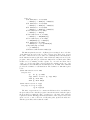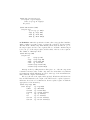
1
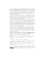
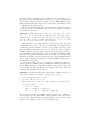
Refinement and Theorem Proving⋆
Panagiotis Manolios
College of Computing
Georgia Institute of Technology
Atlanta, GA, 30318
[email protected]
1
Introduction
In this chapter, we describe the ACL2 theorem proving system and show how it
can be used to model and verify hardware using refinement.
This is a timely problem, as the ever-increasing complexity of microprocessor designs and the potentially devastating economic consequences of shipping
defective products has made functional verification a bottleneck in the microprocessor design cycle, requiring a large amount of time, human effort, and resources [1, 58]. For example, the 1994 Pentium FDIV bug cost Intel $475 million
and it is estimated that a similar bug in the current generation Intel Pentium
processor would cost Intel $12 billion [2].
One of the key optimizations used in these designs is pipelining, a topic
that has received a fair amount of interest from the research community. In this
chapter, we show how to define a pipelined machine in ACL2 and how to use
refinement to verify that it correctly implements its instruction set architecture.
We discuss how to automate such proofs using theorem proving, decision procedures, and hybrid approaches that combine these two methods. We also outline
future research directions.
2
The ACL2 Theorem Proving System
“ACL2” stands for “A Computational Logic for Applicative Common Lisp.” It
is the name of a programming language, a first-order mathematical logic based
on recursive functions, and a mechanical theorem prover for that logic.
ACL2 is an industrial-strength version of the Boyer-Moore theorem prover [5]
and was developed by Kaufmann and Moore , with early contributions by Robert
Boyer; all three developers were awarded the 2005 ACM Software System Award
for their work. Of special note is its “industrial-strength”: as a programming
language, it executes so efficiently that formal models written in it have been used
as simulation platforms for pre-fabrication requirements testing; as a theorem
prover, it has been used to prove the largest and most complicated theorems ever
⋆
This research was funded in part by NSF grants CCF-0429924, IIS-0417413, and
CCF-0438871.
proved about commercially designed digital artifacts. In this section we give an
informal overview of the ACL2 system.
The sources for ACL2 are freely available on the Web, under the GNU
General Public License. The ACL2 homepage is http://www.cs.utexas.edu/users/moore/acl2 [26]. Extensive documentation, including tutorials, a user’s
manual, workshop proceedings, and related papers are available from the ACL2
homepage. ACL2 is also described in a textbook by Kaufmann, Manolios, and
Moore [23]. There is also a book of case studies [22]. Supplementary material for
both books, including all the solutions to the exercises (over 200 in total) can
be found on the Web [25, 24].
We recently released ACL2s [13], a version of ACL2 that features a modern graphical integrated development environment in Eclipse, levels appropriate for beginners through experts, state-of-the-art enhancements such as our
recent improvements to termination analysis [45], etc. ACL2s is available at
http://www.cc.gatech.edu/home/manolios/acl2s and is being developed with
the goal of making formal reasoning accessible to the masses, with an emphasis
on building a tool that any undergraduate can profitably use in a short amount
of time. The tool includes many features for streamlining the learning process
that are not found in ACL2. In general, the goal is to develop a tool that is
“self-teaching,” i.e., it should be possible for an undergraduate to sit down and
play with it and learn how to program in ACL2 and how to reason about the
programs she writes.
ACL2, the language, is an applicative, or purely functional programming
language. The ACL2 data types and expressions are presented in sections 2.1 and
2.2, respectively. A consequence of the applicative nature of ACL2 is that the rule
of Leibniz, i.e., x = y ⇒ f.x = f.y, written in ACL2 as (implies (equal x
y) (equal (f x) (f y))), is a theorem. This effectively rules out side effects.
Even so, ACL2 code can be made to execute efficiently. One way is to compile
ACL2 code, which can be done with any Common Lisp [59] compiler. Another
way is to use stobjs, single-threaded objects. Logically, stobjs have applicative
semantics, but syntactic restrictions on their use allow ACL2 to produce code
that destructively modifies stobjs. Stobjs have been very useful when efficiency is
paramount, as is the case when modeling complicated computing systems such as
microprocessors. For example, Hardin, Wilding, and Greve compare the speeds
of a C model and an ACL2 model of the JEM1 (a silicon Java Virtual Machine
designed by Rockwell Collins). They found that the ACL2 model runs at about
90% of the speed of the C model [16].
ACL2, the logic, is a first-order logic. The logic can be extended with events;
examples of events are function definitions, constant definitions, macro definitions, and theorems. Logically speaking, function definitions introduce new
axioms. Since new axioms can easily render the theory unsound, ACL2 has a
definitional principle which limits the kinds of functions one can define. For example, the definitional principle guarantees that functions are total , i.e., that
they terminate. ACL2 also has macros, which allow one to customize the syntax.
In section 2.3 we discuss the issues.
We give a brief overview of how the theorem prover works in section 2.4. We
also describe encapsulation, a mechanism for introducing constrained functions,
functions that satisfy certain constraints, but that are otherwise undefined. We
end section 2.4 by describing books in section 2.4. Books are files of events that
often contain libraries of theorems and can be loaded by ACL2 quickly, without
having to prove theorems.
In section 2.5 we list some of the applications to which ACL2 has been
applied. We end in section 2.6, by showing, in detail, how to model hardware in
ACL2. We do this by defining a simple, but not trivial, pipelined machine and
its instruction set architecture.
2.1
Data Types
The ACL2 universe consists of atoms and conses. Atoms are atomic objects and
include the following.
1. Numbers includes integers, rationals, and complex rationals. Examples include -1, 3/2, and #c(-1 2).
2. Characters represent the ASCII characters. Examples include #\2, #\a, and
#\Space.
3. Strings are finite sequences of characters; an example is "Hello World!".
4. Symbols consist of two strings: a package name and a symbol name. For
example, the symbol FOO::BAR has package name "FOO" and symbol name
"BAR". ACL2 is case-insensitive with respect to symbol and package names.
If a package name is not given, then the current package name is used, e.g.,
if the current package is "FOO", then BAR denotes the symbol FOO::BAR. The
symbols t and nil are used to denote true and false, respectively.
Conses are ordered pairs of objects. For example, the ordered pair consisting
of the number 1 and the string "A" is written (X . "X"). The left component
of a cons is called the car and the right component is called the cdr. You can
think of conses as binary trees; the cons (X . "X") is depicted in figure 1(a).
Of special interest are a class of conses called true lists. A true list is either
the symbol nil, which denotes the empty list and can be written (), or a cons
whose cdr is a true list. For example, the true list containing the numbers 0 and
1
2 , written (0 1/2), is depicted in figure 1(b). Also of interest are association
lists or alists. An alist is a true list of conses and is often used to represent a
mapping that associates the car of an element in the list with its cdr. The alist
((X . 3) (Y . 2)) is shown in figure 1(c).
2.2
Expressions
Expressions, which are also called terms, represent ACL2 programs and evaluate
to ACL2 objects. We give an informal overview of expressions in this section.
This allows us to suppress many of the details while focusing on the main ideas.
Expressions depend on what we call a history, a list recording events. One reason
(a)
X
"X"
(b)
(c)
0
1/2 nil
X
3
Y
(X . "X")
(0 1/2)
2
nil
((X . 3) (Y . 2))
Fig. 1. Examples of conses.
for this dependency is that it is possible to define new functions (see section 2.3
on page 7) and these new functions can be used to form new expressions. User
interaction with ACL2 starts in what we call the ground-zero history which
includes an entry for the built-in functions. As new events arise, the history is
extended, e.g., a function definition extends the history with an entry, which
includes the name of the function and its arity. We are now ready to discuss
expressions. Essentially, given history h, an expression is:
– A constant symbol, which includes the symbols t, nil, and symbols in the
package "KEYWORD"; constant symbols evaluate to themselves.
– A constant expression, which is a number, a character, a string, or a quoted
constant, a single quote (’) followed by an object. Numbers, characters, and
strings evaluate to themselves. The value of a quoted constant is the object
quoted. For example, the values of 1, #\A, "Hello", ’hello, and ’(1 2 3)
are 1, #\A, "Hello", (the symbol) hello, and (the list) (1 2 3), respectively.
– A variable symbol, which is any symbol other than a constant symbol. The
value of a variable symbol is determined by an environment.
– A function application, (f e1 . . . en ), where f is a function expression of
arity n in history h and ei , for 1 ≤ i ≤ n, is an expression in history h.
A function expression of arity n is a symbol denoting a function of arity
n (in history h) or a lambda expression of the form (lambda (v1 . . . vn )
body), where v1 , . . . , vn are distinct, body is an expression (in history h), and
the only variables occurring freely in body are v1 , . . . , vn . The value of the
expression is obtained by evaluating function f in the environment where
the values of v1 , . . . , vn are e1 , . . . , en , respectively.
ACL2 contains many built-in, or primitive, functions. For example, cons is a
built-in function of two arguments that returns a cons whose left element is the
value of the first argument and whose right element is the value of the second
argument. Thus, the value of the expression (cons ’x 3) is the cons (x . 3)
because the value of the quoted constant ’x is the symbol x and the value of the
constant 3 is itself. Similarly, the value of expression (cons (cons nil ’(cons
a 1)) (cons ’x 3)) is ((nil . (cons a 1)) . (x . 3)). There are built-in
functions for manipulating all of the ACL2 data types. Some of the built-in
functions are described in table 1.
Expression
(equal x y)
(if x y z)
(implies x y)
(not x)
(acl2-numberp x)
(integerp x)
(rationalp x)
(atom x)
(endp x)
(zp x)
(consp x)
(car x)
(cdr x)
(cons x y)
Value
T if the value of x equals the value of y, else nil
The value of z if the value of x is nil, else the value of y
T if the value of x is nil or the value of y is not nil, else nil
T if the value of x is nil, else nil
T if the value of x is a number, else nil
T if the value of x is an integer, else nil
T if the value of x is a rational number, else nil
T if the value of x is an atom, else nil
Same as (atom x)
T if the value of x is 0 or is not a natural number, else nil
T if the value of x is a cons, else nil
If the value of x is a cons, its left element, else nil
If the value of x is a cons, its right element, else nil
A cons whose car is the value of x and whose cdr is
the value of y
(binary-append x y) The list resulting from concatenating the value of x
and the value of y
(len x)
The length of the value of x, if it is a cons, else 0
Table 1. Some built-in function symbols and their values.
Comments are written with the use of semicolons: anything following a semicolon, up to the end of the line on which the semicolon appears, is a comment.
Notice that an expression is an (ACL2) object and that an object is the value of
some expression. For example, the object (if (consp x) (car x) nil) is the
value of the expression ’(if (consp x) (car x) nil).
Expressions also include macros, which are discussed in more detail in section 2.3. Macros are syntactic sugar and can be used to define what seem to
be functions of arbitrary arity. For example, + is a macro that can be used as
if it is a function of arbitrary arity. We can write (+), (+ x), and (+ x y z)
which evaluate to 0, the value of x, and the sum of the values of x, y, and z,
respectively. The way this works is that binary-+ is a function of two arguments
and expressions involving + are abbreviations for expressions involving 0 or more
occurrences of binary-+, e.g., (+ x y z) is an abbreviation for (binary-+ x
(binary-+ y z)).
Commonly used macros include the ones listed in table 2.
An often used macro is cond. Cond is a generalization of if. Instead of
deciding between two expressions based on one test, as happens with if, one
Expression
Value
(caar x)
The car of the car of x
(cadr x)
The car of the cdr of x
(cdar x)
The cdr of the car of x
(cddr x)
The cdr of the cdr of x
(first x)
The car of x
(second x)
The cadr of x
(append x1 . . . xn) The binary-append of x1 . . . xn
(list x1 . . . xn) The list containing x1 . . . xn
(+ x1 . . . xn)
Addition
(* x1 . . . xn)
Multiplication
(- x y)
Subtraction
(and x1 . . . xn)
Logical conjunction
(or x1 . . . xn)
Logical disjunction
Table 2. Some commonly used macros and their values.
can decide between any number of expressions based on the appropriate number
of tests. Here is an example.
(cond (test1 exp1 )
...
(testn expn )
(t expn+1 ))
The above cond is an abbreviation for the following expression.
(if test1 exp1
...
(if testn expn
expn+1 ) . . . )
Another important macro is let. Let expressions are used to (simultaneously) bind values to variables and expand into lambdas. For example
(let ((v1
...
(vn
body)
e1 )
en ))
is an abbreviation for
((lambda (v1 . . . vn )
body)
e1 . . . en )
Consider the expression (let ((x ’(1 2)) (y ’(3 4))) (append x y)).
It is an abbreviation for ((lambda (x y) (binary-append x y)) ’(1 2) ’(3
4)), whose value is the list (1 2 3 4).
Finally, let* is a macro that is used to sequentially bind values to variables
and can be defined using let, as we now show.
(let* ((v1
...
(vn
body)
e1 )
en ))
is an abbreviation for
(let ((v1 e1 ))
(let* (. . .
(vn en ))
body))
2.3
Definitions
In this section, we give an overview of how one goes about defining new functions
and macros in ACL2.
Functions Functions are defined using defun. For example, we can define the
successor function, a function of one argument that increments its argument by
1, as follows.
(defun succ (x)
(+ x 1))
The form of a defun is (defun f doc dcl1 . . . dclm (x1 . . . xn ) body), where:
x1 . . . xn are distinct variable symbols
the free variables in body are in x1 . . . xn
doc is a documentation string and is optional
dcl1 . . . dclm are declarations and are optional
functions, other than f , used in body have been previously introduced
body is an expression in the current history, extended to allow function applications of f
– if f is recursive we must prove that it terminates
–
–
–
–
–
–
A common use of declarations is to declare guards. Guards are used to indicate the expected domain of a function. Since ACL2 is a logic of total functions,
all functions, regardless of whether there are guard declarations or not, are defined on all ACL2 objects. However, guards can be used to increase efficiency
because proving that guards are satisfied allows ACL2 to directly use the underlying Common Lisp implementation to execute functions. For example, endp
and eq are defined as follows.
(defun endp (x)
(declare (xargs :guard (or (consp x) (equal x nil))))
(atom x))
(defun eq (x y)
(declare (xargs :guard (if (symbolp x) t (symbolp y))))
(equal x y))
Both endp and eq are logically equivalent to atom and equal, respectively. The
only difference is in their guards, as atom and equal both have the guard t. If
eq is only called when one of its arguments is a symbol, then it can be implemented more efficiently than equal, which can be called on anything, including
conses, numbers, and strings. Guard verification consists of proving that defined
functions respect the guards of the functions they call. If guards are verified,
then ACL2 can use efficient versions of functions.
Another common use of declarations is to declare the measure used to prove
termination of a function. Consider the following function definition.
(defun app (x y)
(declare (xargs :measure (len x)))
(if (consp x)
(cons (car x) (app (cdr x) y))
y))
App is a recursive function that can be used to concatenate lists x and y. Such a
definition introduces the axiom (app x y) = body where body is the body of the
function definition. The unconstrained introduction of such axioms can render
the theory unsound, e.g., consider the “definition” (defun bad (x) (not (bad
x))). The axiom introduced, namely, (bad x) = (not (bad x)) allows us to
prove nil (false). To guarantee that function definitions are meaningful, ACL2
has a definitional principle which requires that the we prove that the function
terminates. This requires exhibiting a measure, an expression that decreases on
each recursive call of the function. For many of the common recursion schemes,
ACL2 can guess the measure. In the above example, we explicitly provide a
measure for function app using a declaration. The measure is the length of x.
Notice that app is called recursively only if x is a cons and it is called on the
cdr of x, hence the length of x decreases. For an expression to be a measure, it
must evaluate to an ACL2 ordinal on any argument. ACL2 ordinals correspond
to the ordinals up to ǫ0 in set theory [43, 41, 42, 44]. They allow one to use many
of the standard well-founded structures commonly used in termination proofs,
e.g., the lexicographic ordering on tuples of natural numbers [42].
Macros Macros are really useful for creating specialized notation and for abbreviating commonly occurring expressions. Macros are functions on ACL2 objects,
but they differ from ACL2 functions in that they map the objects given as arguments to expressions, whereas ACL2 functions map the values of the objects
given as arguments to objects. For example, if m is a macro then (m x1 . . .
xn ) may evaluate to an expression obtained by evaluating the function corresponding to the macro symbol m on arguments x1 , . . . , xn (not their values,
as happens with function evaluation), obtaining an expression exp. Exp is the
immediate expansion of (m x1 . . . xn ) and is then further evaluated until no
macros remain, resulting in the complete expansion of the term. The complete
expansion is then evaluated, as described previously.
Suppose that we are defining recursive functions whose termination can be
shown with measure (len x), where x is the first argument to the function.
Instead of adding the required declarations to all of the functions under consideration, we might want to write a macro that generates the required defun.
Here is one way of doing this.
(defmacro defunm (name args body)
‘(defun ,name
,args
(declare (xargs :measure (len ,(first args))))
,body))
Notice that we define macros using defmacro, in a manner similar to function
definitions. Notice the use of what is called the backquote notation. The value
of a backquoted list is a list that has the same structure as the backquoted list
except that expressions preceded by a comma are replaced by their values. For
example, if the value of name is app, then the value of ‘(defun ,name) is (defun
app).
We can now use defunm as follows.
(defunm app (x y)
(if (consp x)
(cons (car x) (app (cdr x) y))
y))
This expands to the following.
(defun app (x y)
(declare (xargs :measure (len x)))
(if (consp x)
(cons (car x) (app (cdr x) y))
y))
When the above is processed, the result is that the function app is defined. In
more detail, the above macro is evaluated as follows. The macro formals name,
args, and body are bound to app, (x y), and (if (consp x) (cons (car x)
(app (cdr x) y)) y), respectively. Then, the macro body is evaluated. As per
the discussion on the backquote notation, the above expansion is produced.
We consider a final example to introduce ampersand markers. The example
is the list macro and its definition follows.
(defmacro list (&rest args)
(list-macro args))
Recall that (list 1 2) is an abbreviation for (cons 1 (cons 2 nil)). In addition, list can be called on an arbitrary number of arguments; this is accomplished with the use of the &rest ampersand marker. When this marker is used,
it results in the next formal, args, getting bound to the list of the remaining arguments. Thus, the value of (list 1 2) is the value of the expression
(list-macro ’(1 2)). In this way, an arbitrary number of objects are turned
into a single object, which is passed to the function list-macro, which in the
above case returns the expression (cons 1 (cons 2 nil)).
2.4
The Theorem Prover
The ACL2 theorem prover is an integrated system of ad hoc proof techniques
that include simplification, generalization, induction and many other techniques.
Simplification is, however, the key technique. The typewriter font keywords
below refer to online documentation topics accessible from the ACL2 online
user’s manual [26]. The simplifier includes the use of (1) evaluation (i.e., the
explicit computation of constants when, in the course of symbolic manipulation, certain variable-free expressions, like (expt 2 32), arise), (2) conditional
rewrite rules (derived from previously proved lemmas), cf. rewrite, (3) definitions (including recursive definitions), cf. defun, (4) propositional calculus (implemented both by the normalization of if-then-else expressions and the use of
BDDs), cf. bdd, (5) a linear arithmetic decision procedure for the rationals (with
extensions to help with integer problems and with non-linear problems [17]), cf.
linear-arithmetic, (6) user-defined equivalence and congruence relations, cf.
equivalence, (7) user-defined and mechanically verified simplifiers, cf. meta, (8)
a user-extensible type system, cf. type-prescription, (9) forward chaining, cf.
forward-chaining, (10) an interactive loop for entering proof commands, cf.
proof-checker, and (11) various means to control and monitor these features
including heuristics, interactive features, and user-supplied functional programs.
The induction heuristic, cf. induction, automatically selects an induction
based on the recursive patterns used by the functions appearing in the conjecture or a user-supplied hint. It may combine various patterns to derive a “new”
one considered more suitable for the particular conjecture. The chosen induction scheme is then applied to the conjecture to produce a set of new subgoals,
typically including one or more base cases and induction steps. The induction
steps typically contain hypotheses identifying a particular non-base case, one
or more instances of the conjecture to serve as induction hypotheses, and, as
the conclusion, the conjecture being proved. The system attempts to select an
induction scheme that will provide induction hypotheses that are useful when
the function applications in the conclusion are expanded under the case analysis
provided. Thus, while induction is often considered the system’s forte, most of
the interesting work, even for inductive proofs, occurs in the simplifier.
We now discuss how to prove theorems with ACL2. All of the system’s proof
techniques are sensitive to the database of previously proved rules, included in
the logical world or world and, if any, user-supplied hints. By proving appropriate
theorems (and tagging them in pragmatic ways) it is possible to make the system
expand functions in new ways, replace one term by another in certain contexts,
consider unusual inductions, add new known inequalities to the linear arithmetic
procedure, restrict generalizations, etc.
The command for submitting theorems to ACL2 is defthm. Here is an example.
(defthm app-is-associative
(equal (app (app x y) z)
(app x (app y z))))
ACL2 proves this theorem automatically, given the definition of app, but with
more complicated theorems ACL2 often needs help. One way of providing help
is to prove lemmas which are added to the world and can then be used in
future proof attempts. For example, ACL2 does not prove the following theorem
automatically.
(defthm app-is-associative-with-one-arg
(equal (app (app x x) x)
(app x (app x x))))
However, if app-is-associative is in the world, then ACL2 recognizes that the
above theorem follows (it is a special case of app-is-associative). Another way
of providing help is to give explicit hints, e.g., one can specify what induction
scheme to use, or what instantiations of previously proven theorems to use, and
so on. More generally, the form of a defthm is
(defthm name formula
:rule-classes (class1 . . . classn )
:hints . . .)
where both the :rule-classes and :hints parts are optional.
Encapsulation ACL2 provides a mechanism called encapsulation
by which
one can introduce constrained functions. For example, the following event can
be used to introduce a function that is constrained to be associative and commutative.
(encapsulate
(((ac * *) => *))
(local (defun ac (x y) (+ x y)))
(defthm ac-is-associative
(equal (ac (ac x y) z)
(ac x (ac y z))))
(defthm ac-is-commutative
(equal (ac x y)
(ac y x))))
This event adds the axioms ac-is-associative and ac-is-commutative. The
sole purpose of the local definition of ac in the above encapsulate form is to
establish that the constraints are satisfiable. In the world after admission of the
encapsulate event, the function ac is undefined; only the two constraint axioms
are known.
There is a derived rule of inference called functional instantiation that is used
as follows. Suppose f is a constrained function with constraint φ and suppose
that we prove theorem ψ. Further suppose that g is a function that satisfies
the constraint φ, with f replaced by g, then replacing f by g in ψ results in a
theorem as well. That is, any theorem proven about f holds for any function
satisfying the constraints on f . For example, we can prove the following theorem
about ac. Notice that we had to provide hints to ACL2.
(defthm commutativity-2-of-ac
(equal (ac y (ac x z))
(ac x (ac y z)))
:hints (("Goal"
:in-theory (disable ac-is-associative)
:use ((:instance ac-is-associative)
(:instance ac-is-associative
(x y) (y x))))))
We can now use the above theorem and the derived rule of inference to show
that any associative and commutative function satisfies the above theorem. For
example, here is how we show that * satisfies the above theorem.
(defthm commutativity-2-of-*
(equal (* y (* x z))
(* x (* y z)))
:hints (("Goal"
:by (:functional-instance
commutativity-2-of-ac
(ac (lambda (x y) (* x y)))))))
ACL2 generates and establishes the necessary constraints, that * is associative
and commutative.
Encapsulation and functional instantiation allow quantification over functions and thus have the flavor of a second order mechanism, although they are
really first-order. For the full details see [4, 29].
Books A book is a file of ACL2 events analogous to a library. The ACL2 distribution comes with many books, including books for arithmetic, set theory, data
structures, and so on. The events in books are certified as admissible and can
be loaded into subsequent ACL2 sessions without having to replay the proofs.
This makes it possible to structure large proofs and to isolate related theorems
into libraries. Books can include local events that are not included when books
are included, or loaded, into an ACL2 session.
2.5
Applications
ACL2 has been applied to a wide range of commercially interesting verification
problems. We recommend visiting the ACL2 home page [26] and inspecting the
links on Tours, Demo, Books and Papers, and for the most current work, The
Workshops and Related Meetings. See especially [22]. ACL2 has been used on
various large projects, including the verification of floating point [48, 50, 52,
51, 53], microprocessor verification [18, 19, 7, 20, 56, 57, 54, 15, 14, 16, 8], and
programming languages [47, 3]. There are various papers describing aspects the
internals of ACL2, including single-threaded objects [6], encapsulation [29], and
the base logic [27].
2.6
Modeling Hardware
In this section, we show how to model a simple machine both at the instruction
set architecture (ISA) level and at the microarchitecture (MA) level. The MA
machine is roughly based on Sawada’s simple machine [55, 54] and the related
machines appearing in [30, 31]. It contains a three-stage pipeline and in the
sequel, we will be interested in verifying that it “correctly” implements the ISA
machine.
The ISA machine has instructions that are four-tuples consisting of an opcode, a target register, and two source registers. The MA machine is a pipelined
machine with three stages. A pipeline is analogous to an assembly line. The
pipeline consists of several stages each of which performs part of the computation required to complete an instruction. When the pipeline is full many instructions are in various degrees of completion. A diagram of the MA machine
appears in Fig. 2. The three stages are fetch, set-up, and write. During the fetch
stage, the instruction pointed to by the PC (program counter) is retrieved from
memory and placed into latch 1. During the set-up stage, the contents of the
source registers (of the instruction in latch 1) are retrieved from the register file
and sent to latch 2 along with the rest of the instruction in latch 1. During the
write stage, the appropriate ALU (arithmetic logic unit) operation is performed
and the result is used to update the value of the target register.
Register
File
PC
Latch
2
Latch
1
ALU
Memory
Fig. 2. Our simple three-stage pipeline machine.
Let us consider a simple example where the contents of memory are as follows.
Inst
0
1
add
add
rb
ra
ra
rb
ra
ra
When this simple two-line code fragment is executed on the ISA and MA
machines, we get the following traces, where we only show the value of the
program counter and the contents of registers ra and rb.
Clock
0
1
2
3
4
5
ISA
MA
h0, h1, 1ii h0, h1, 1ii
h1, h1, 2ii h1, h1, 1ii
h2, h3, 2ii h2, h1, 1ii
h2, h1, 2ii
h , h1, 2ii
h , h3, 2ii
Inst 0
Fetch
Set-up
Write
Inst 1
Fetch
Stall
Set-up
Write
The rows correspond to steps of the machines, e.g., row Clock 0 corresponds
to the initial state, Clock 1 to the next state, and so on. The ISA and MA
columns contain the relevant parts of the state of the machines: a pair consisting
of the PC and the register file (itself a pair consisting of registers ra and rb). The
final two columns indicate what stage the instructions are in (only applicable to
the MA machine).
In the initial state (in row Clock 0) the PCs of the ISA and MA machines
contain the value 0 (indicating that the next instruction to execute is Inst 0) and
both registers have the value 1. In the next ISA state (in row Clock 1), the PC is
incremented and the add instruction performed, i.e., register rb is updated with
the value ra + ra = 2. The final entry in the ISA column contains the state of
the ISA machine after executing Inst 1.
After one step of the MA machine, Inst 0 completes the fetch phase and the
PC is incremented to point to the next instruction. After step 2 (in row Clock 2),
Inst 0 completes the set-up stage, Inst 1 completes the fetch phase, and the PC is
incremented. After step 3, Inst 0 completes the write-back phase and the register
file is updated for the first time with rb set to 2. However, Inst 1 is stalled during
step 3 because one of its source registers is rb, the target register of the previous
instruction. Since the previous instruction has not completed, the value of rb is
not available and Inst 1 is stalled for one cycle. In the next cycle, Inst 1 enters
the set-up stage and Inst 2 enters the fetch stage (not shown). Finally, after
step 5, Inst 1 is completed and register ra is updated.
ISA Definition We now consider how to define the ISA and MA machines
using ACL2. The first machine we define is ISA. The main function is ISA-step,
a function that steps the ISA machine, i.e., it takes an ISA state and returns the
next ISA state. The definition of ISA-step follows.
(defun ISA-step (ISA)
(let ((inst (g (g :pc ISA) (g :imem ISA))))
(let ((op (g :opcode inst))
(rc (g :rc
inst))
(ra (g :ra
inst))
(rb (g :rb
inst)))
(case op
(add (ISA-add rc ra rb ISA))
;; REGS[rc] := REGS[ra] + REGS[rb]
(sub (ISA-sub rc ra rb ISA))
;; REGS[rc] := REGS[ra] - REGS[rb]
(mul (ISA-mul rc ra rb ISA))
;; REGS[rc] := REGS[ra] * REGS[rb]
(load (ISA-load rc ra ISA))
;; REGS[rc] := MEM[ra]
(loadi (ISA-loadi rc ra ISA))
;; REGS[rc] := MEM[REGS[ra]]
(store (ISA-store ra rb ISA))
;; MEM[REGS[ra]] := REGS[rb]
(bez (ISA-bez ra rb ISA))
;; REGS[ra]=0 -> pc:=pc+REGS[rb]
(jump (ISA-jump ra ISA))
;; pc:=REGS[ra]
(otherwise (ISA-default ISA))))))
The ISA-step function uses a book (library) for reasoning about records. One
of the functions exported by the records books is g (get), where (g f r) gets
the value of field f from record r. Therefore, ISA-step fetches the instruction
in the instruction memory (the field :imem of ISA state ISA) referenced by the
program counter (the field :pc of ISA state ISA) and stores this in inst, which
itself is a record consisting of fields :opcode, :rc, :ra, and :rb. Then, based
on the opcode, the appropriate action is taken. For example, in the case of an
add instruction, the next ISA state is (ISA-add rc ra rb ISA), where ISA-add
provides the semantics of add instructions. The definition of ISA-add is given
below
(defun ISA-add (rc ra rb ISA)
(seq-isa nil
:pc
(1+ (g :pc ISA))
:regs (add-rc ra rb rc (g :regs ISA))
:imem (g :imem ISA)
:dmem (g :dmem ISA)))
(defun add-rc (ra rb rc regs)
(seq regs rc (+ (g ra regs)
(g rb regs))))
The macro seq-isa is used to construct an ISA state whose four fields have
the given values. Notice that the program counter is incremented and the register
file is updated by setting the value of register rc to the sum of the values in
registers ra and rb. This happens in fuction add-rc, where seq is a macro that
given a record, r, and a collection of field/value pairs, updates the fields in r
with the given values and returns the result.
The other ALU instructions are similarly defined. We now show how to define
the semantics of the rest of the instructions (ifix forces its argument to be an
integer).
(defun ISA-loadi (rc ra ISA)
(let ((regs (g :regs ISA)))
(seq-isa nil
:pc
(1+ (g :pc ISA))
:regs (load-rc (g ra regs) rc regs (g :dmem ISA))
:imem (g :imem ISA)
:dmem (g :dmem ISA))))
(defun load-rc (ad rc regs dmem)
(seq regs rc (g ad dmem)))
(defun ISA-load (rc ad ISA)
(seq-isa nil
:pc
(1+ (g :pc ISA))
:regs (load-rc ad rc (g :regs ISA) (g :dmem ISA))
:imem (g :imem ISA)
:dmem (g :dmem ISA)))
(defun ISA-store
(seq-isa nil
:pc
:regs
:imem
:dmem
(ra rb ISA)
(1+ (g :pc ISA))
(g :regs ISA)
(g :imem ISA)
(store ra rb (g :regs ISA) (g :dmem ISA))))
(defun store (ra rb regs dmem)
(seq dmem (g ra regs) (g rb regs)))
(defun ISA-jump (ra ISA)
(seq-isa nil
:pc (ifix (g ra (g :regs ISA)))
:regs (g :regs ISA)
:imem (g :imem ISA)
:dmem (g :dmem ISA)))
(defun ISA-bez (ra rb ISA)
(seq-isa nil
:pc (bez ra rb (g :regs ISA) (g :pc ISA))
:regs (g :regs ISA)
:imem (g :imem ISA)
:dmem (g :dmem ISA)))
(defun bez (ra rb regs pc)
(if (equal 0 (g ra regs))
(ifix (+ pc (g rb regs)))
(1+ pc)))
(defun ISA-default (ISA)
(seq-isa nil
:pc (1+ (g :pc
:regs (g :regs
:imem (g :imem
:dmem (g :dmem
ISA))
ISA)
ISA)
ISA)))
MA Definition ISA is the specification for MA, a three stage pipelined machine,
which contains a program counter, a register file, a memory, and two latches.
The first latch contains a flag which indicates if the latch is valid, an opcode,
the target register, and two source registers. The second latch contains a flag as
before, an opcode, the target register, and the values of the two source registers.
The definition of MA-step follows.
(defun MA-step (MA)
(seq-ma nil
:pc
(step-pc MA)
:regs
(step-regs MA)
:dmem
(step-dmem MA)
:imem
(g :imem MA)
:latch1 (step-latch1 MA)
:latch2 (step-latch2 MA)))
MA-step works by calling functions that given one of the MA components
return the next state value of that component. Note that this is very different
from ISA-step, which calls functions, based on the type of the next instruction,
that return the complete next ISA state.
Below, we show how the register file is updated. If latch2 is valid, then if we
have an ALU instruction, the output of the ALU is used to update register rc.
Otherwise, if we have a load instruction, then we update register rc with the
appropriate word from memory.
(defun step-regs (MA)
(let* ((regs
(g :regs MA))
(dmem
(g :dmem MA))
(latch2
(g :latch2 MA))
(validp
(g :validp latch2))
(op
(g :op latch2))
(rc
(g :rc latch2))
(ra-val
(g :ra-val latch2))
(rb-val
(g :rb-val latch2)))
(if validp
(cond ((alu-opp op)
(seq regs rc (ALU-output op ra-val rb-val)))
((load-opp op)
(seq regs rc (g ra-val dmem)))
(t regs))
regs)))
(defun alu-opp (op)
(in op ’(add sub mul)))
(defun load-opp (op)
(in op ’(load loadi)))
(defun in (x y)
(if (endp y)
nil
(or (equal x (car y))
(in x (cdr y)))))
(defun ALU-output (op val1 val2)
(cond ((equal op ’add)
(+ val1 val2))
((equal op ’sub)
(- val1 val2))
(t (* val1 val2))))
We now show how to update latch2. If latch1 is not valid or if it will be stalled,
then latch2 is invalidated. Othewise, we copy the :op and :rc fields from latch1
and read the contents of registers :rb and :ra, except for load instructions. The
:pch field is a history variable: it does not affect the computation of the machine
and is used only to aid the proof process. We use one more history variable in
latch1. Both history variables serve the same purpose: they are used to record
the address of the instruction with which they are associated.
(defun step-latch2 (MA)
(let* ((latch1 (g :latch1 MA))
(l1op
(g :op latch1)))
(if (or (not (g :validp latch1))
(stall-l1p MA))
(seq-l2 nil :validp nil)
(seq-l2 nil
:validp t
:op
l1op
:rc
(g :rc latch1)
:ra-val (if (equal l1op ’load)
(g :ra latch1)
(g (g :ra latch1) (g :regs MA)))
:rb-val (g (g :rb latch1) (g :regs MA))
:pch
(g :pch latch1)))))
We update latch1 as follows. If it will be stalled then, it stays the same. If
it will be invalidated, then it is. Otherwise, we fetch the next instruction from
memory and store it in the register (and record the address of the instruction
in the history variable :pch). Latch1 is stalled exactly when it and latch2 are
valid and latch2 contains an instruction that will modify one of the registers
latch1 depends on. Latch1 is invalidated if it contains any branch instruction
(because the jump address cannot be determined yet) or if latch2 contains a bez
instruction (again, the jump address cannot be determined for bez instructions
until the instruction has made its way through the pipeline, whereas the jump
address for jump instructions can be computed during the second stage of the
machine).
(defun step-latch1 (MA)
(let ((latch1 (g :latch1 MA))
(inst
(g (g :pc MA) (g :imem MA))))
(cond ((stall-l1p MA)
latch1)
((invalidate-l1p MA)
(seq-l1 nil :validp nil))
(t (seq-l1 nil
:validp t
:op
(g :opcode inst)
:rc
(g :rc inst)
:ra
(g :ra inst)
:rb
(g :rb inst)
:pch
(g :pc MA))))))
(defun stall-l1p (MA)
(let* ((latch1
(g :latch1 MA))
(l1validp (g :validp latch1))
(latch2
(g :latch2 MA))
(l1op
(g :op latch1))
(l2op
(g :op latch2))
(l2validp (g :validp latch2))
(l2rc
(g :rc latch2))
(l1ra
(g :ra latch1))
(l1rb
(g :rb latch1)))
(and l2validp l1validp
(rc-activep l2op)
(or (equal l1ra l2rc)
(and (uses-rbp l1op)
(equal l1rb l2rc))))))
(defun rc-activep (op)
(or (alu-opp op)
(load-opp op)))
(defun uses-rbp (op)
(or (alu-opp op)
(in op ’(store bez))))
(defun uses-rbp (op)
(or (alu-opp op)
(in op ’(store bez))))
(defun invalidate-l1p (MA)
(let* ((latch1
(g :latch1 MA))
(l1op
(g :op latch1))
(l1validp (g :validp latch1))
(latch2
(g :latch2 MA))
(l2op
(g :op latch2))
(l2validp (g :validp latch2)))
(or (and l1validp
(in l1op ’(bez jump)))
(and l2validp
(equal l2op ’bez)))))
Memory is updated only when we have a store instruction, in which case
we update the memory appropriately.
(defun step-dmem (MA)
(let* ((dmem
(g :dmem MA))
(latch2
(g :latch2 MA))
(l2validp (g :validp latch2))
(l2op
(g :op latch2))
(l2ra-val (g :ra-val latch2))
(l2rb-val (g :rb-val latch2)))
(if (and l2validp (equal l2op ’store))
(seq dmem l2ra-val l2rb-val)
dmem)))
Finally, the program counter is updated as follows. If latch1 will stall, then
the program counter is not modified. Otherwise, if latch1 will be invalidated,
then if this is due to a bez instruction in latch2, the jump address can be now
be determined, so the program counter is updated as per the semantics of the
bez instruction. Otherwise, if the invalidation is due to a jump instruction in
latch1, the jump address can be computed and the program counter is set to
this address. The only other possibility is that the invalidation is due to a bez
instruction in latch1; in this case the jump address has not yet been determined,
so the pc is not modified. Note, this simple machine does not have a branch
predictor. If the invalidate signal does not hold, then we increment the program
counter unless we are fetching a branch instruction.
(defun step-pc (MA)
(let* ((pc
(g :pc MA))
(inst
(g (g :pc MA) (g :imem MA)))
(op
(g :opcode inst))
(regs
(g :regs MA))
(latch1
(g :latch1 MA))
(l1op
(g :op latch1))
(latch2
(g :latch2 MA))
(l2op
(g :op latch2))
(l2validp (g :validp latch2))
(l2ra-val (g :ra-val latch2))
(l2rb-val (g :rb-val latch2)))
(cond ((stall-l1p MA)
pc)
((invalidate-l1p MA)
(cond ((and l2validp
(equal l2op ’bez))
(if (equal 0 l2ra-val)
(ifix (ALU-output ’add pc l2rb-val))
(1+ pc)))
((equal l1op ’jump)
(ifix (g (g :ra latch1) regs)))
(t pc)))
;;; must be bez instruction
((in op ’(jump bez))
pc)
(t (1+ pc)))))
This ends the description of the ISA and MA machines. To summarize, we
can use ACL2 to define machines models at any level of abstraction we like.
What we wind up with are simulators for the machines, which we can execute.
For example, consider the following program to multiply x and y (without using
the mul instruction). The data memory contains the constants 0, 1, 4, and 6 in
memory locations 0, 1, 4, and 6, respectively. It also contains x and y in memory
locations 2 and 3.
(defun mul-dmem (x y)
(seq nil 0 0 1 1 2 x 3 y 4 4 6 6))
The instruction memory contains the following code.
(defun inst (op rc ra rb)
(seq nil :opcode op :rc rc :ra ra :rb rb))
(defun mul-imem ()
(seq nil
0
1
2
3
4
5
6
7
8
9
(inst
(inst
(inst
(inst
(inst
(inst
(inst
(inst
(inst
(inst
’load 0 1 nil)
’load 1 2 nil)
’load 2 3 nil)
’load 3 0 nil)
’load 4 4 nil)
’load 6 6 nil)
’bez nil 1 4)
’sub 1 1 0)
’add 3 3 2)
’jump nil 6 nil)))
The code works by adding x copies of y in register 3. For example (isa-run
(isa-state 0 nil (mul-imem) (mul-dmem 3 4)) 19) is an ISA state whose
:pc is 10 (indicating exit from the loop) and with a value of 12 in register 3. Similarly, (ma-run (ma-state 0 nil (mul-imem) (mul-dmem 3 4) nil
nil) 30) is the corresponding MA state.
3
Refinement
In the previous section, we saw how one can model a pipelined machine and
its instruction set architecture in ACL2. We now discuss how to verify such
machines. Consider the partial traces of the ISA and MA machines on the simple
two-line code fragment from the previous section (add rb ra ra followed by
add ra rb ra). We are only showing the value of the program counter and the
contents of registers ra and rb.
ISA
h0, h1,1ii
h1, h1,2ii
h2, h3,2ii
MA
h0, h1,1ii
h1, h1,1ii
h2, h1,1ii
h2, h1,2ii
h , h1,2ii
h , h3,2ii
→
Commit
PC
h0,
h0,
h0,
h1,
h1,
h2,
MA
h1,1ii
h1,1ii
h1,1ii
h1,2ii
h1,2ii
h3,2ii
→
Remove
Stutter
MA
h0, h1,1ii
h1, h1,2ii
h2, h3,2ii
Notice that the PC differs in the two traces and this occurs because the
pipeline, initially empty, is being filled and the PC points to the next instruction
to fetch. If the PC were to point to the next instruction to commit (i.e., the next
instruction to complete), then we would get the trace shown in column 3. Notice
that in column 3, the PC does not change from 0 to 1 until Inst 0 is committed
in which case the next instruction to commit is Inst 1. We now have a trace that
is the same as the ISA trace except for stuttering; after removing the stuttering
we have, in column 4, the ISA trace.
We now formalize the above and start with the notion of a refinement map,
a function that maps MA states to ISA states. In the above example we mapped
MA states to ISA states by transforming the PC. Proving correctness amounts
to relating MA states with the ISA states they map to under the refinement map
and proving a WEB (Well-founded Equivalence Bisimulation). Proving a WEB
guarantees that MA states and related ISA states have related computations up
to finite stuttering. This is a strong notion of equivalence, e.g., a consequence is
that the two machines satisfy the same CTL∗ \ X properties.1 This includes the
class of next-time free safety and liveness (including fairness) properties, e.g.,
one such property is that the MA machine cannot deadlock (because the ISA
machine cannot deadlock).
Why “up to finite stuttering”? Because we are comparing machines at different levels of abstraction: the pipelined machine is a low-level implementation of
the high-level ISA specification. When comparing systems at different levels of
abstraction, it is often the case that the low-level system requires several steps
to match a single step of the high-level system.
Why use a refinement map? Because there may be components in one system
that do not appear in the other, e.g., the MA machine has latches but the ISA
machine does not. In addition, data can be represented in different ways, e.g., a
pipelined machine might use binary numbers whereas its instruction set architecture might use a decimal representation. Yet another reason is that components
present in both systems may have different behaviors, as is the case with the
PC above. Notice that the refinement map affects how MA and ISA states are
related, not the behavior of the MA machine.
The theory of refinement we present is based on transition systems (TSs). A
TS, M, is a triple hS, 99K, Li, consisting of a set of states, S, a left-total transition
relation, 99K⊆ S 2 , and a labeling function L whose domain is S and where L.s
(we sometimes use an infix dot to denote function application) corresponds to
what is “visible” at state s. Clearly, the ISA and MA machines can be thought of
as transition systems (TS).
Our notion of refinement is based on the following definition of stuttering
bisimulation [9], where by fp(σ, s) we mean that σ is a fullpath (infinite path)
starting at s, and by match(B, σ, δ) we mean that the fullpaths σ and δ are
equivalent sequences up to finite stuttering (repetition of states).
Definition 1. B ⊆ S × S is a stuttering bisimulation (STB) on TS M =
hS, 99K,Li iff B is an equivalence relation and for all s, w such that sBw:
(Stb1)
L.s = L.w
(Stb2)
h∀σ : fp(σ, s) : h∃δ : fp(δ, w) : match(B, σ, δ)ii
Browne, Clarke, and Grumberg have shown that states that are stuttering
bisimilar satisfy the same next-time-free temporal logic formulas [9].
Lemma 1. Let B be an STB on M and let sBw. For any CTL∗ \ X formula f ,
M, w |= f iff M, s |= f .
We note that stuttering bisimulation differs from weak bisimulation [46]
in that weak bisimulation allows infinite stuttering. Stuttering is a common
1
CTL∗ is a braching-time temporal logic; CTL∗ \ X is CTL∗ without the next-time
operator X .
phenomenon when comparing systems at different levels of abstraction, e.g., if
the pipeline is empty, MA will require several steps to complete an instruction,
whereas ISA completes an instruction during every step. Distinguishing between
infinite and finite stuttering is important, because (among other things) we want
to distinguish deadlock from stutter.
When we say that MA refines ISA, we mean that in the disjoint union (⊎) of
the two systems, there is an STB that relates every pair of states w, s such that
w is an MA state and r(w) = s.
Definition 2. (STB Refinement) Let M = hS, 99K, Li, M′ = hS ′ , 99K′ , L′ i,
and r : S → S ′ . We say that M is a STB refinement of M′ with respect to
refinement map r, written M ≈r M′ , if there exists a relation, B, such that
h∀s ∈ S :: sBr.si and B is an STB on the TS hS ⊎ S ′ , 99K ⊎ 99K′ , Li, where
L.s = L′ .s for s an S ′ state and L.s = L′ (r.s) otherwise.
STB refinement is a generally applicable notion. However, since it is based
on bisimulation, it is often too strong a notion and in this case refinement based
on stuttering simulation should be used (see [32, 33]). The reader may be surprised that STB refinement theorems can be proved in the context of pipelined
machine verification; after all, features such as branch prediction can lead to
non-deterministic pipelined machines, whereas the ISA is deterministic. While
this is true, the pipelined machine is related to the ISA via a refinement map
that hides the pipeline; when viewed in this way, the nondeterminism is masked
and we can prove that the two systems are stuttering bisimilar (with respect to
the ISA visible components).
A major shortcoming of the above formulation of refinement is that it requires reasoning about infinite paths, something that is difficult to automate [49].
In [32], WEB-refinement, an equivalent formulation is given that requires only
local reasoning, involving only MA states, the ISA states they map to under the
refinement map, and their successor states.
Definition 3. Well-Founded Equivalence Bisimulation (WEB [34, 49]) B is a
well-founded equivalence bisimulation on TS M = hS, 99K, Li iff:
1. B is an equivalence relation on S; and
2. h∀s, w ∈ S : sBw : L.s = L.wi; and
3. There exists function erank : S × S → W, with hW, ≺i well-founded, and
h∀s, u, w ∈ S : sBw ∧ s 99K u :
h∃v : w 99K v : uBvi ∨
(uBw ∧ erank (u, u) ≺ erank (s, s)) ∨
h∃v : w 99K v : sBv ∧ erank (u, v) ≺ erank (u, w)ii
We call a pair hrank , hW, ≺ii satisfying condition 3 in the above definition, a
well-founded witness. The third WEB condition guarantees that related states
have the same computations up to stuttering. If states s and w are in the same
class and s can transit to u, then one of the following holds.
1. The transition can be matched with no stutter, in which case, u is matched
by a step from w.
2. The transition can be matched but there is stutter on the left (from s), in
which case, u and w are in the same class and the rank function decreases
(to guarantee that w is forced to take a step eventually).
3. The transition can be matched but there is stutter on the right (from w),
in which case, there is some successor v of w in the same class as s and the
rank function decreases (to guarantee that u is eventually matched).
To prove a relation is a WEB, note that reasoning about single steps of 99K
suffices. In addition we can often get by with a rank function of one argument.
Note that the notion of WEB refinement is independent of the refinement
map used. For example, we can use the standard flushing refinement map [11],
where MA states are mapped to ISA states by executing all partially completed
instructions without fetching any new instructions, and then projecting out the
ISA visible components. In previous work, we have explored the use of other
refinement maps, e.g., in [39, 38, 21], we present new classes of refinement maps
that can provide several orders of magnitude improvements in verification times
over the standard flushing-based refinement maps. In this paper, however, we
use the commitment refinement map, introduced in [30].
A very important property of WEB refinement is that it is compositional,
something that we have exploited in several different contexts [40, 37].
Theorem 1. (Composition) If M ≈r M′ and M′ ≈q M′′ then M ≈r;q M′′ .
Above, r; q denotes composition, i.e., (r; q)(s) = q(r.s).
From the above theorem we can derive several other composition results; for
example:
Theorem 2. (Composition)
MA ≈r · · · ≈q ISA
ISA k P ⊢ ϕ
MA k P ⊢ ϕ
In this form, the above rule exactly matches the compositional proof rules in [12].
The above theorem states that to prove MA k P ⊢ ϕ (that MA, the pipelined machine, executing program P satisfies property ϕ, a property over the ISA visible
state), it suffices to prove MA ≈ ISA and ISA k P ⊢ ϕ: that MA refines ISA (which
can be done using a sequence of refinement proofs) and that ISA, executing P ,
satisfies ϕ. That is, we can prove that code running on the pipelined machine
is correct, by first proving that the pipelined machine refines the instruction
set architecture and then proving that the software running on the instruction
set—not on the pipelined machine—is correct.
4
Pipelined Machine Verification
In this section, we show how to use ACL2 to prove the correctness of the pipelined
machine we have defined, using WEB-refinement. We start, in section 4.1 by
discussing how we deal with quantification in ACL2. We then discuss how the
refinement maps are defined, in section 4.2. Finally, in section 4.3, we discuss
the proof of correctness.
4.1
Quantification
The macro defun-sk is used to implement quantification in ACL2 by introducing witness functions and constraints. For example, the quantified formula
h∃x :: P (x, y)i is expressed in ACL2 as the function EP with the constraints (P x
y) ⇒ (EP y) and (EP y) = (P (W y) y). To see that this corresponds to quantification, notice that the first constraint gives us one direction of the argument:
it says that if any value of x makes (P x y) true (i.e., if h∃x :: P (x, y)i) then
(EP y) is true. This constraint allows us to establish an existentially quantified
formula by exhibiting a witness, but the constraint can be satisfied if EP always
returns t. The second constraint gives us the other direction. It introduces the
witness function W and requires that (EP y) is true iff (P (W y) y) is true.
As a result, if (EP y) is true, then some value of x makes (P x y) true. As is
mentioned in the ACL2 documentation [26], this idea was known to Hilbert.
We wish to use quantification and encapsulation in the following way. We
prove that a set of constrained functions satisfy a quantified formula. We then
use functional instantiation to show that a set of functions satisfying these constraints also satisfy the (analogous) quantified formula. We want this proof obligation to be generated by macros but have found that the constraints generated
by the quantified formulas complicate the design of such macros. The following observation has allowed us to simplify the process. The quantified formulas
are established using witness functions, as is often the case. Therefore, only the
first constraint generated by defun-sk is required for the proof. We defined the
macro defun-weak-sk which generates only this constraint, e.g., the following
(defun-weak-sk E (y)
(exists (x) (P x y)))
leads only to the constraint that (P x y) ⇒ (E y). By functional instantiation,
any theorem proved about E also holds when E is replaced by EP (since EP satisfies
the constraint on E). We use defun-weak-sk in our scripts and at the very end
we prove the defun-sk versions of the main results by functional instantiation
(a step taken to make the presentation of the final result independent of our
macros).
4.2
Refinement Map Definitions
To prove that MA is a correct implementation of ISA, we prove a WEB on the
(disjoint) union of the machines, with MA states labeled by the appropriate refinement map. Once the required notions are defined, the macros implementing our
proof methodology can be used to prove correctness without any user supplied
theorems. In this section, we present the definitions which make the statement
of correctness precise.
The following function is a recognizer for “good” MA states.
(defun good-MA (ma)
(and (integerp (g :pc MA))
(let* ((latch1 (g :latch1 MA))
(latch2 (g :latch2 MA))
(nma (committed-ma ma)))
(cond ((g :validp latch2)
(equiv-ma (ma-step (ma-step nma)) ma))
((g :validp latch1)
(equiv-ma (ma-step nma) ma))
(t t)))))
First, we require that pc, the program counter, is an integer. Such type restrictions are common. Next, we require that MA states are reachable from clean states
(states with invalid latches). The reason for this restriction is that otherwise MA
states can be inconsistent (unreachable), e.g., consider an MA state whose first
latch contains an add instruction, but where there are no add instructions in
memory. We check for this by stepping the committed state, the state obtained
by invalidating all partially completed instructions and altering the program
counter so that it points to the next instruction to commit.
(defun committed-MA (MA)
(let* ((pc
(g :pc MA))
(latch1
(g :latch1 MA))
(latch2
(g :latch2 MA)))
(seq-ma nil :pc
(committed-pc latch1 latch2 pc)
:regs
(g :regs MA)
:dmem
(g :dmem MA)
:imem
(g :imem MA)
:latch1 (seq-l1 nil)
:latch2 (seq-l2 nil))))
The program counter of the committed state is obtained from the history variable
of the first valid latch.
(defun committed-pc (l1 l2 pc)
(cond ((g :validp l2)
(g :pch l2))
((g :validp l1)
(g :pch l1))
(t pc)))
Finally, we note that equiv-MA relates two MA states if they have the same pc,
regs, memories, and if their latches match, i.e., they have equivalent latch 1s or
both states have an invalid latch 1 and similarly with latch 2.
Note that committed-MA invalidates pending instructions and adjusts the
program counter accordingly. To make sure that a state is not inconsistent, we
check that it is reachable from the corresponding committed state. Now that we
have made precise what the MA states are, the refinement map is:
(defun MA-to-ISA (MA)
(let ((MA (committed-MA
(seq-isa nil :pc
(g
:regs (g
:dmem (g
:imem (g
MA)))
:pc MA)
:regs MA)
:dmem MA)
:imem MA))))
The final definition required is that of the well-founded witness. The function
MA-rank serves this purpose by computing how long it will take an MA state to
commit an instruction. An MA state will commit an instruction in the next step
if its second latch is valid. Otherwise, if its first latch is valid it will be ready
to commit an instruction in one step. Otherwise, both latches are invalid and it
will be ready to commit an instruction in two steps.
(defun MA-rank (MA)
(let ((latch1 (g :latch1 MA))
(latch2 (g :latch2 MA)))
(cond ((g :validp latch2)
0)
((g :validp latch1)
1)
(t 2))))
4.3
Proof of Correctness
To complete the proof we have to define the machine corresponding to the disjoint union of ISA and MA, define a WEB that relates a (good) MA state s to
(MA-to-ISA s), define the well-founded witness, and prove that indeed the purported WEB really is a WEB. We have implemented macros which automate
this. The macros are useful not only for this example, but have also been used
to verification many other machines, including machines defined at the bit level.
(Non-deterministic versions have also been developed that can be used to reason
about machines with interrupts [31, 30].) The proof of correctness is completed
with the following three macro calls.
(generate-full-system isa-step isa-p ma-step ma-p
ma-to-isa good-ma ma-rank)
(prove-web isa-step isa-p ma-step ma-p ma-to-isa ma-rank)
(wrap-it-up isa-step isa-p ma-step ma-p good-ma
ma-to-isa ma-rank)
The first macro, generate-full-system, generates the definition of B, the
purported WEB, as well as R, the transition relation of the disjoint union of the
ISA and MA machines. The macro translates to the following. (Some declarations
and forward-chaining theorems used to control the theorem prover have been
elided.)
(progn
(defun wf-rel (x y)
(and (ISA-p x)
(MA-p y)
(good-MA y)
(equal x (MA-to-ISA y))))
(defun B (x y)
(or (wf-rel x y)
(wf-rel y x)
(equal x y)
(and (MA-p x)
(MA-p y)
(good-MA x)
(good-MA y)
(equal (MA-to-ISA x) (MA-to-ISA y)))))
(defun rank (x)
(if (MA-p x) (MA-rank x) 0))
(defun R (x y)
(cond ((ISA-p x) (equal y (ISA-step x)))
(t (equal y (MA-step x))))))
What is left is to prove that B—the reflexive, symmetric, transitive closure
of wf-rel—is a WEB with well-founded witness rank. We do this in two steps.
First, the macro prove-web is used to prove the “core” theorem (as well as some
“type” theorems not shown).
(defthm B-is-a-wf-bisim-core
(let ((u (ISA-step s))
(v (MA-step w)))
(implies (and (wf-rel s w)
(not (wf-rel u v)))
(and (wf-rel s v)
(o< (MA-rank v) (MA-rank w))))))
Comparing B-is-a-wf-bisim-core with the definition of WEBs, we see that
B-is-a-wf-bisim-core does not contain quantifiers and it mentions neither B
nor R. This is on purpose as we use “domain-specific” information to construct
a simplified theorem that is used to establish the main theorem. To that end
we removed the quantifiers and much of the case analysis. For example, in the
definition of WEBs, u ranges over successors of s and v is existentially quantified
over successors of w, but because we are dealing with deterministic systems, u
and v are defined to be the successors of s and w, respectively. Also, wf-rel is
not an equivalence relation as it is not reflexive, symmetric, or transitive. Finally,
we ignore the second disjunct in the third condition of the definition of WEBs
because ISA does not stutter. The justification for calling this the “core” theorem
is that we have proved in ACL2 that a constrained system which satisfies a
theorem analogous to B-is-a-wf-bisim-core (and some “type” theorems) also
satisfies a WEB. Using functional instantiation we can now prove MA correct.
The use of this domain-specific information makes a big difference, e.g., when
we tried to prove the theorem obtained by a naive translation of the WEB
definition (sans quantifiers), ACL2 ran out of memory after many hours, yet the
above theorem is now proved in about 1,000 seconds.
The final macro call generates the events used to finish the proof. We present
the generated events germane to this discussion below. The first step is to show
that B is an equivalence relation. This theorem is proved by functional instantiation.
(defequiv B
:hints (("goal" :by (:functional-instance
encap-B-is-an-equivalence . . .))))
The second WEB condition, that related states have the same label, is taken
care of by the refinement map. We show that rank is a well-founded witness.
(defthm rank-well-founded
(o-p (rank x)))
We use functional instantiation and B-is-a-wf-bisim-core as described
above to prove the following.
(defun-weak-sk exists-w-succ-for-u-weak (w u)
(exists (v) (and (R w v) (B u v))))
(defun-weak-sk exists-w-succ-for-s-weak (w s)
(exists (v)
(and (R w v)
(B s v)
(o< (rank v) (rank w)))))
(defthm B-is-a-wf-bisim-weak
(implies (and (B s w)
(R s u))
(or (exists-w-succ-for-u-weak w u)
(and (B u w)
(o< (rank u) (rank s)))
(exists-w-succ-for-s-weak w s)))
:hints
(("goal" :by (:functional-instance
B-is-a-wf-bisim-sk . . .)))
:rule-classes nil)
We use defun-weak-sk for these definitions for the reasons outlined in Section 4.1. Stating the result in terms of the built-in macro defun-sk involves a
trivial functional instantiation (since the single constraint generated by defun-weak-sk
is one of the constraints generated by defun-sk).
(defun-sk exists-w-succ-for-u (w u)
(exists (v) (and (R w v) (B u v))))
(defun-sk exists-w-succ-for-s (w s)
(exists (v)
(and (R w v)
(B s v)
(o< (rank v) (rank w)))))
(defthm B-is-a-wf-bisim
(implies (and (B s w)
(R s u))
(or (exists-w-succ-for-u w u)
(and (B u w)
(o< (rank u) (rank s)))
(exists-w-succ-for-s w s)))
:hints
(("goal"
:by
(:functional-instance b-is-a-wf-bisim-weak
(exists-w-succ-for-u-weak exists-w-succ-for-u)
(exists-w-succ-for-s-weak exists-w-succ-for-s))))
:rule-classes nil))
5
Verifying Complex Machines
While the proof of the pipelined machine defined in this paper required little
more than writing down the correctness statement, unfortunately, using theorem proving to verify more complicated machines requires heroic effort [54]. The
second major approach to the pipeline machine verification problem is based
on decision procedures such as UCLID [10]. UCLID is a tool that decides the
CLU logic, a logic containing the boolean connectives, uninterpreted functions
and predicates, equality, counter arithmetic, ordering, and restricted lambda
expressions. This approach is very automatic, e.g., in a carefully constructed
experiment, problems that took ACL2 days took seconds with UCLID [36]. Unfortunately, this approach has several problems. For example, pipelined machines
that exceed the complexity threshold of the tools used, which happens rather easily, cannot be analyzed. Another serious limitation is that the pipelined machine
models used are term-level models: they abstract away the datapath, implement
a small subset of the instruction set, require the use of numerous abstractions,
and are far from executable. Nonetheless, one can automatically handle much
more complex machines with decision procedures than one can handle with general purpose theorem provers. In this section, we discuss some of our current
work on this topic, as well as directions for future work.
5.1
Automating Verification of Term-Level Machines
In [35], it is shown how to automate the refinement proofs in the context of termlevel pipelined machine verification. The idea is to strengthen, thereby simplifying, the refinement proof obligation; the result is the CLU-expressible formula,
where rank is a function that maps states of MA into the natural numbers. MA
≈r ISA if:
h∀w ∈ MA ::
=⇒
s = r.w ∧ u = ISA-step(s) ∧
v = MA-step(w) ∧ u 6= r.v
s = r.v ∧ rank .v < rank .wi
In the formula above s and u are ISA states, and w and v are MA states; ISA-step
is a function corresponding to stepping the ISA machine once and MA-step is a
function corresponding to stepping the MA machine once. It may help to think
of the first conjunct of the consequent (s = r.v) as the safety component of the
proof and the second conjunct rank .v < rank .w as the liveness component.
5.2
Compositional Reasoning
We have developed a compositional reasoning framework based on refinement
that consists of a set of convenient, easily-applicable, and complete compositional
proof rules [37]. Our framework greatly extends the applicability of decision
procedures, e.g., we were able to verify, in seconds, a complex, deeply pipelined
machine that state-of-the-art tools cannot currently handle. Our framework can
be added to the design cycle, which is also compositional. In addition, one of
the most important benefits of our approach over current methods is that the
counterexamples generated tend to be much simpler, in terms of size and number
of simulation steps involved and can be generated much more quickly.
5.3
Combining ACL2 and UCLID
The major problem with approaches based on decision procedures is that they
only work for abstract term-level models and do not provide a firm connection
with RTL models. In order to be industrially useful, we need both automation
and a connection to the RTL level. As an initial step towards verifying RTLlevel designs, we have combined ACL2 and UCLID in order to verify pipelined
machine models with bit-level interfaces [40]. We use ACL2 to reduce the proof
that an executable, bit-level machine refines its instruction set architecture to a
proof that a term level abstraction of the bit-level machine refines the instruction
set architecture, which is then handled automatically by UCLID. The amount
of effort required is about 3-4 times the effort required to prove the term-level
model correct using only UCLID. This allows us to exploit the strengths of ACL2
and UCLID to prove theorems that are not possible to even state using UCLID
and that would require prohibitively more effort using just ACL2.
5.4
Conclusion and Future Perspectives
We view our work on compositional reasoning and on combining ACL2 and
UCLID as promising first steps. Clearly, compositional reasoning will be needed
to allow us to handle the verification problems one component at a time. With
regard to RTL-level reasoning, our work has shown that we can automate the
problem to within a small constant factor of what can be done for term-level
models, but it will be important to change the factor to 1+ε. Several ideas for doing this include: developing a pattern database that with some intelligent search
that can automatically decompose verification problems, automating some of the
simpler refinement steps we currently perform, using counter-example guided
abstraction-refinement to automatically abstract RTL designs to term-level designs, automating the handling of memories and register files, improved decision
procedures, and creating analyses that work directly on hardware description
languages.
References
[1] B. Bentley. Validating the Intel Pentium 4 microprocessor. In 38th Design Automation Conference, pages 253–255, 2001.
[2] B. Bentley. Validating a modern microprocessor, 2005. See URL http://www.cav2005.inf.ed.ac.uk/bentley CAV 07 08 2005.ppt.
[3] P. Bertoli and P. Traverso. Design verification of a safety-critical embedded verifier. In Kaufmann et al. [22], pages 233–245.
[4] R. S. Boyer, D. M. Goldschlag, M. Kaufmann, and J. S. Moore. Functional
instantiation in first order logic. In V. Lifschitz, editor, Artificial Intelligence and
Mathematical Theory of Computation: Papers in Honor of John McCarthy, pages
7–26. Academic Press, 1991.
[5] R. S. Boyer and J. S. Moore. A Computational Logic Handbook. Academic Press,
second edition, 1997.
[6] R. S. Boyer and J. S. Moore.
Single-threaded objects in ACL2,
1999.
See URL http://www.cs.utexas.edu/users/moore/publications/acl2-papers.html#Foundations.
[7] B. Brock and W. A. Hunt, Jr. Formally specifying and mechanically verifying
programs for the Motorola complex arithmetic processor DSP. In 1997 IEEE
International Conference on Computer Design, pages 31–36. IEEE Computer Society, Oct. 1997.
[8] B. Brock, M. Kaufmann, and J. S. Moore. ACL2 theorems about commercial
microprocessors. In M. Srivas and A. Camilleri, editors, Formal Methods in
Computer-Aided Design (FMCAD’96), pages 275–293. Springer-Verlag, 1996.
[9] M. Browne, E. M. Clarke, and O. Grumberg. Characterizing finite Kripke structures in propositional temporal logic. Theoretical Computer Science, 59, 1988.
[10] R. E. Bryant, S. K. Lahiri, and S. Seshia. Modeling and verifying systems using a
logic of counter arithmetic with lambda expressions and uninterpreted functions.
In E. Brinksma and K. Larsen, editors, Computer-Aided Verification–CAV 2002,
volume 2404 of LNCS, pages 78–92. Springer-Verlag, 2002.
[11] J. R. Burch and D. L. Dill. Automatic verification of pipelined microprocessor
control. In Computer-Aided Verification (CAV ’94), volume 818 of LNCS, pages
68–80. Springer-Verlag, 1994.
[12] E. M. Clarke, O. Grumberg, and D. Peled. Model Checking. MIT Press, 1999.
[13] P. Dillinger, P. Manolios, , and D. Vroon. ACL2s homepage. See URL http://www.cc.gatech.edu/home/manolios/acl2s.
[14] D. Greve, M. Wilding, and D. Hardin. High-speed, analyzable simulators. In
Kaufmann et al. [22], pages 113–135.
[15] D. A. Greve. Symbolic simulation of the JEM1 microprocessor. In Formal Methods
in Computer-Aided Design – FMCAD, LNCS. Springer-Verlag, 1998.
[16] D. Hardin, M. Wilding, and D. Greve. Transforming the theorem prover into
a digital design tool: From concept car to off-road vehicle. In A. J. Hu and
M. Y. Vardi, editors, Computer-Aided Verification – CAV ’98, volume 1427 of
LNCS. Springer-Verlag, 1998. See URL http://pobox.com/users/hokie/docs/concept.ps.
[17] W. Hunt, R. Krug, and J. S. Moore. The addition of non-linear arithmetic to
ACL2. In D. Geist, editor, Proceedings of CHARME 2003, volume 2860 of Lecture
Notes in Computer Science, pages 319–333. Springer Verlag, 2003.
[18] W. A. Hunt, Jr. Microprocessor design verification. Journal of Automated Reasoning, 5(4):429–460, 1989.
[19] W. A. Hunt, Jr. and B. Brock. A formal HDL and its use in the FM9001 verification. Proceedings of the Royal Society, 1992.
[20] W. A. Hunt, Jr. and B. Brock. The DUAL-EVAL hardware description language and
its use in the formal specification and verification of the FM9001 microprocessor.
Formal Methods in Systems Design, 11:71–105, 1997.
[21] R. Kane, P. Manolios, and S. K. Srinivasan. Monolithic verification of deep
pipelines with collapsed flushing. In Design Automation and Test in Europe,
DATE’06, 2006.
[22] M. Kaufmann, P. Manolios, and J. S. Moore, editors. Computer-Aided Reasoning:
ACL2 Case Studies. Kluwer Academic Publishers, June 2000.
[23] M. Kaufmann, P. Manolios, and J. S. Moore. Computer-Aided Reasoning: An
Approach. Kluwer Academic Publishers, July 2000.
[24] M. Kaufmann, P. Manolios, and J. S. Moore. Supporting files for “ComputerAided Reasoning: ACL2 Case Studies”. See the link from URL http://www.cs.utexas.edu/users/moore/acl2, 2000.
[25] M. Kaufmann, P. Manolios, and J. S. Moore. Supporting files for “ComputerAided Reasoning: An Approach”. See the link from URL http://www.cs.utexas.edu/users/moore/acl2, 2000.
[26] M. Kaufmann and J. S. Moore. ACL2 homepage. See URL http://www.cs.utexas.edu/users/moore/acl2.
[27] M. Kaufmann and J. S. Moore. A precise description of the ACL2 logic. Technical report, Department of Computer Sciences, University of Texas at Austin,
1997.
See URL http://www.cs.utexas.edu/users/moore/publications/acl2-papers.html#Foundations.
[28] M. Kaufmann and J. S. Moore, editors. Proceedings of the ACL2 Workshop 2000.
The University of Texas at Austin, Technical Report TR-00-29, November 2000.
[29] M. Kaufmann and J. S. Moore. Structured theory development for a mechanized
logic. Journal of Automated Reasoning, 26(2):161–203, February 2001.
[30] P. Manolios. Correctness of pipelined machines. In W. A. Hunt, Jr. and S. D.
Johnson, editors, Formal Methods in Computer-Aided Design–FMCAD 2000, volume 1954 of LNCS, pages 161–178. Springer-Verlag, 2000.
[31] P. Manolios. Verification of pipelined machines in ACL2. In Kaufmann and Moore
[28].
[32] P. Manolios. Mechanical Verification of Reactive Systems. PhD thesis, University of Texas at Austin, August 2001. See URL http://www.cc.gatech.edu/∼manolios/publications.html.
[33] P. Manolios. A compositional theory of refinement for branching time. In D. Geist
and E. Tronci, editors, 12th IFIP WG 10.5 Advanced Research Working Conference, CHARME 2003, volume 2860 of LNCS, pages 304–318. Springer-Verlag,
2003.
[34] P. Manolios, K. Namjoshi, and R. Sumners. Linking theorem proving and modelchecking with well-founded bisimulation. In N. Halbwachs and D. Peled, editors,
Computer-Aided Verification–CAV ’99, volume 1633 of LNCS, pages 369–379.
Springer-Verlag, 1999.
[35] P. Manolios and S. Srinivasan. Automatic verification of safety and liveness for
XScale-like processor models using WEB-refinements. In Design Automation and
Test in Europe, DATE’04, pages 168–175, 2004.
[36] P. Manolios and S. Srinivasan. A suite of hard ACL2 theorems arising in
refinement-based processor verification. In M. Kaufmann and J. S. Moore, editors,
Fifth International Workshop on the ACL2 Theorem Prover and Its Applications
(ACL2-2004), November 2004. See URL http://www.cs.utexas.edu/users/moore/acl2/workshop-2004/.
[37] P. Manolios and S. Srinivasan. A complete compositional reasoning framework
for the efficient verification of pipelined machines. In ICCAD-2005, International
Conference on Computer-Aided Design, 2005.
[38] P. Manolios and S. Srinivasan. A computationally efficient method based on commitment refinement maps for verifying pipelined machines models. In ACM-IEEE
International Conference on Formal Methods and Models for Codesign, pages 189–
198, 2005.
[39] P. Manolios and S. Srinivasan. Refinement maps for efficient verification of processor models. In Design Automation and Test in Europe, DATE’05, pages 1304–
1309, 2005.
[40] P. Manolios and S. Srinivasan. Verification of executable pipelined machines with
bit-level interfaces. In ICCAD-2005, International Conference on Computer-Aided
Design, 2005.
[41] P. Manolios and D. Vroon. Algorithms for ordinal arithmetic. In F. Baader, editor,
19th International Conference on Automated Deduction – CADE-19, volume 2741
of LNAI, pages 243–257. Springer–Verlag, July/August 2003.
[42] P. Manolios and D. Vroon. Ordinal arithmetic in ACL2. In M. Kaufmann and J. S.
Moore, editors, Fourth International Workshop on the ACL2 Theorem Prover and
Its Applications (ACL2-2003), July 2003. See URL http://www.cs.utexas.edu/users/moore/acl2/workshop-2003/.
[43] P. Manolios and D. Vroon. Integrating reasoning about ordinal arithmetic into
ACL2. In Formal Methods in Computer-Aided Design: 5th International Conference – FMCAD-2004, LNCS. Springer–Verlag, November 2004.
[44] P. Manolios and D. Vroon. Ordinal arithmetic: Algorithms and mechanization.
Journal of Automated Reasoning, 2006. to appear.
[45] P. Manolios and D. Vroon. Termination analysis with calling context graphs,
2006. Submitted.
[46] R. Milner. Communication and Concurrency. Prentice-Hall, 1990.
[47] J. S. Moore. Piton : A Mechanically Verified Assembly-Level Language. Kluwer
Academic Press, Dordrecht, The Netherlands, 1996.
[48] J. S. Moore, T. Lynch, and M. Kaufmann. A mechanically checked proof of the
AMD5K 86 floating-point division program. IEEE Trans. Comp., 47(9):913–926,
September 1998.
[49] K. S. Namjoshi. A simple characterization of stuttering bisimulation. In 17th Conference on Foundations of Software Technology and Theoretical Computer Science,
volume 1346 of LNCS, pages 284–296, 1997.
[50] D. M. Russinoff. A mechanically checked proof of correctness of the AMD5K 86
floating-point square root microcode. Formal Methods in System Design Special
Issue on Arithmetic Circuits, 1997.
[51] D. M. Russinoff. A mechanically checked proof of IEEE compliance of a registertransfer-level specification of the AMD-K7 floating-point multiplication, division,
and square root instructions. London Mathematical Society Journal of Computation and Mathematics, 1:148–200, December 1998.
[52] D. M. Russinoff. A mechanically checked proof of correctness of the AMD-K5
floating-point square root microcode. Formal Methods in System Design, 14:75–
125, 1999.
[53] D. M. Russinoff and A. Flatau. RTL verification: A floating-point multiplier. In
Kaufmann et al. [22], pages 201–231.
[54] J. Sawada. Formal Verification of an Advanced Pipelined Machine. PhD thesis,
University of Texas at Austin, Dec. 1999. See URL http://www.cs.utexas.edu/users/sawada/dissertation/.
[55] J. Sawada. Verification of a simple pipelined machine model. In Kaufmann et al.
[22], pages 137–150.
[56] J. Sawada and W. A. Hunt, Jr. Trace table based approach for pipelined microprocessor verification. In Computer Aided Verification (CAV ’97), volume 1254
of LNCS, pages 364–375. Springer-Verlag, 1997.
[57] J. Sawada and W. A. Hunt, Jr. Processor verification with precise exceptions and
speculative execution. In A. J. Hu and M. Y. Vardi, editors, Computer Aided
Verification (CAV ’98), volume 1427 of LNCS, pages 135–146. Springer-Verlag,
1998.
[58] International technology roadmap for semiconductors, 2004. See URL http://public.itrs.net/.
[59] G. L. Steele, Jr. Common Lisp The Language, Second Edition. Digital Press,
Burlington, MA, 1990.