Download Nesl: A Nested Data-Parallel Language (Version 3.1)

Nesl: A Nested Data-Parallel Language
(Version 3.1)
Guy E. Blelloch
September 19, 1995
CMU-CS-95-170
(Updated version of CMU-CS-92-103, January 1992, and CMU-CS-93-129, April 1993)
School of Computer Science
Carnegie Mellon University
Pittsburgh, PA 15213
This research was sponsored in part by the Wright Laboratory, Aeronautical Systems Center, Air Force
Materiel Command, USAF, and the Advanced Research Projects Agency (ARPA) under grant number
F33615-93-1-1330. It was also supported in part by an NSF Young Investigator Award under grant number
CCR-9258525, and by Finmeccanica.
The views and conclusions contained in this document are those of the authors and should not be interpreted
as necessarily representing the official policies or endorsements, either expressed or implied, of Wright
Laboratory or the U. S. Government.
Keywords: Data-parallel, parallel algorithms, supercomputers, nested parallelism,
PRAM model, parallel programming languages, collection-oriented languages.
Abstract
This report describes Nesl, a strongly-typed, applicative, data-parallel language. Nesl
is intended to be used as a portable interface for programming a variety of parallel and
vector computers, and as a basis for teaching parallel algorithms. Parallelism is supplied
through a simple set of data-parallel constructs based on sequences, including a mechanism
for applying any function over the elements of a sequence in parallel and a rich set of parallel
functions that manipulate sequences.
Nesl fully supports nested sequences and nested parallelism—the ability to take a
parallel function and apply it over multiple instances in parallel. Nested parallelism is
important for implementing algorithms with irregular nested loops (where the inner loop
lengths depend on the outer iteration) and for divide-and-conquer algorithms. Nesl also
provides a performance model for calculating the asymptotic performance of a program on
various parallel machine models. This is useful for estimating running times of algorithms
on actual machines and, when teaching algorithms, for supplying a close correspondence
between the code and the theoretical complexity.
This report defines Nesl and describes several examples of algorithms coded in the
language. The examples include algorithms for median finding, sorting, string searching,
finding prime numbers, and finding a planar convex hull. Nesl currently compiles to an
intermediate language called Vcode, which runs on vector multiprocessors (the CRAY
C90 and J90), distributed memory machines (the IBM SP2, Intel Paragon, and Connection
Machine CM-5), and sequential workstations. For many algorithms, the current implementation gives performance close to optimized machine-specific code for these machines.
Note: This report is an updated version of CMU-CS-92-103, which described version 2.4
of the language, and of CMU-CS-93-129, which described version 2.6 of the language. Some
other documents that describe Nesl are:
• The user’s manual [11].
• An overview of the implementation with some timing results [8].
• A formal definition of the Nesl cost model [23].
Contents
1 Introduction
1.1 Parallel Operations on Sequences
1.2 Nested Parallelism . . . . . . . .
1.3 Pairs . . . . . . . . . . . . . . . .
1.4 Types . . . . . . . . . . . . . . .
1.5 Deriving Complexity . . . . . . .
.
.
.
.
.
2
4
8
10
12
13
2 Examples
2.1 String Searching . . . . . . . . . . . . . . . . . . . . . . . . . . . . . . . . .
2.2 Primes . . . . . . . . . . . . . . . . . . . . . . . . . . . . . . . . . . . . . . .
2.3 Planar Convex-Hull . . . . . . . . . . . . . . . . . . . . . . . . . . . . . . .
16
17
18
19
3 Language Definition
3.1 Data . . . . . . . . . . . . . . . . . . . . . .
3.1.1 Atomic Data Types . . . . . . . . .
3.1.2 Sequences ([]) . . . . . . . . . . . .
3.1.3 Record Types (datatype) . . . . . .
3.2 Functions and Constructs . . . . . . . . . .
3.2.1 Conditionals (if) . . . . . . . . . . .
3.2.2 Binding Local Variables (let) . . . .
3.2.3 The Apply-to-Each Construct ({}) .
3.2.4 Defining New Functions (function)
3.2.5 Top-Level Bindings (=) . . . . . . .
22
22
22
24
24
25
25
26
26
28
28
.
.
.
.
.
.
.
.
.
.
.
.
.
.
.
.
.
.
.
.
.
.
.
.
.
.
.
.
.
.
.
.
.
.
.
.
.
.
.
.
.
.
.
.
.
.
.
.
.
.
.
.
.
.
.
.
.
.
.
.
.
.
.
.
.
.
.
.
.
.
.
.
.
.
.
.
.
.
.
.
.
.
.
.
.
.
.
.
.
.
.
.
.
.
.
.
.
.
.
.
.
.
.
.
.
.
.
.
.
.
.
.
.
.
.
.
.
.
.
.
.
.
.
.
.
.
.
.
.
.
.
.
.
.
.
.
.
.
.
.
.
.
.
.
.
.
.
.
.
.
.
.
.
.
.
.
.
.
.
.
.
.
.
.
.
.
.
.
.
.
.
.
.
.
.
.
.
.
.
.
.
.
.
.
.
.
.
.
.
.
.
.
.
.
.
.
.
.
.
.
.
.
.
.
.
.
.
.
.
.
.
.
.
.
.
.
.
.
.
.
.
.
.
.
.
.
.
.
.
.
.
.
.
.
.
.
.
.
.
.
.
.
.
.
.
.
.
.
.
.
.
.
.
.
.
.
.
.
.
.
.
.
.
.
.
.
.
.
.
.
.
.
.
.
.
.
.
.
.
.
.
.
.
.
.
.
.
.
.
.
.
.
.
.
.
Bibliography
29
A The Nesl Grammar
33
B List
B.1
B.2
B.3
B.4
B.5
of Functions
Scalar Functions . . . . . . . . . .
Sequence Functions . . . . . . . . .
Functions on Any Type . . . . . .
Functions for Manipulating Strings
Functions with Side Effects . . . .
.
.
.
.
.
.
.
.
.
.
.
.
.
.
.
.
.
.
.
.
.
.
.
.
.
.
.
.
.
.
.
.
.
.
.
.
.
.
.
.
.
.
.
.
.
.
.
.
.
.
.
.
.
.
.
.
.
.
.
.
.
.
.
.
.
.
.
.
.
.
.
.
.
.
.
.
.
.
.
.
.
.
.
.
.
.
.
.
.
.
.
.
.
.
.
.
.
.
.
.
.
.
.
.
.
.
.
.
.
.
.
.
.
.
.
36
36
41
48
48
49
C Implementation Notes
58
Index
61
1
1
Introduction
This report describes and defines the data-parallel language Nesl. The language was
designed with the following goals:
1. To support parallelism by means of a set of data-parallel constructs
quences. These constructs supply parallelism through (1) the ability
function concurrently over each element of a sequence, and (2) a set of
tions that operate on sequences, such as the permute function, which
order of the elements in a sequence.
based on seto apply any
parallel funcpermutes the
2. To support complete nested parallelism. Nesl fully supports nested sequences, and
the ability to apply any user defined function over the elements of a sequence, even
if the function is itself parallel and the elements of the sequence are themselves sequences. Nested parallelism is critical for describing both divide-and-conquer algorithms and algorithms with nested data structures [7].
3. To generate efficient code for a variety of architectures, including both SIMD and
MIMD machines, with both shared and distributed memory. Nesl currently generates
a portable intermediate code called Vcode [9], which runs on vector multiprocessors
(the CRAY C90 and J90) as well as distributed memory machines (the IBM SP2, Intel
Paragon, and Connection Machine CM-5). Various benchmark algorithms achieve
very good running times on these machines [16, 8].
4. To be well suited for describing parallel algorithms, and to supply a mechanism for
deriving the theoretical running time directly from the code. Each function in Nesl
has two complexity measures associated with it, the work and depth complexities [7].
A simple equation maps these complexities to the asymptotic running time on a
Parallel Random Access Machine (PRAM) Model.
Nesl is a strongly-typed strict first-order functional (applicative) language. It runs
within an interactive environment and is loosely based on the ML language [34]. The
language uses sequences as a primitive parallel data type, and parallelism is achieved exclusively through operations on these sequences [7]. The set of sequence functions supplied by
Nesl was chosen based both on their usefulness on a broad variety of algorithms, and on
their efficiency when implemented on parallel machines. To promote the use of parallelism,
Nesl supplies no serial looping constructs (although serial looping can be simulated with
recursion). NESL has been used for 3 years now for teaching parallel algorithms [10], and
many applications and algorithms have been written in the language [22, 4, 5].
Nesl is the first data-parallel language whose implementation supports nested parallelism. Nested parallelism is the ability to take a parallel function and apply it over multiple
instances in parallel—for example, having a parallel sorting routine, and then using it to
sort several sequences concurrently. The data-parallel languages C* [38], *Lisp [31], and
Fortran 90 [1] (with array extensions) support no form of nested parallelism. The parallel
collections in these languages can only contain scalars or fixed sized records. There is also no
means in these languages to apply a user defined function over each element of a collection.
2
This prohibits the expression of any form of nested parallelism. The languages Connection
Machine Lisp [45], and Paralation Lisp [39] both supply nested parallel constructs, but
no implementation ever supported the parallel execution of these constructs. Blelloch and
Sabot implemented an experimental compiler that supported nested-parallelism for a small
subset of Paralation Lisp [13], but it was deemed near impossible to extend it to the full
language.
A common complaint about high-level data-parallel languages and, more generally, in
the class of languages based on operations over collections [42], such as SETL [40] and
APL [29], is that it can be hard or impossible to determine approximate running times by
looking at the code. As an example, the β primitive in CM-Lisp (a general communication
primitive) is powerful enough that seemingly similar pieces of code could take very different
amounts of time depending on details of the implementation of the operation and of the
data structures. A similar complaint is often made about the language SETL—a language
with sets as a primitive data structure. The time taken by the set operations in SETL
is strongly affected by how the set is represented. This representation is chosen by the
compiler.
For this reason, Nesl was designed so that the built-in functions are quite simple and
so that the asymptotic complexity can be derived from the code. To derive the complexity,
each function in Nesl has two complexity measures associated with it: the work and depth
complexities [7]1 The work complexity represents the serial work executed by a program—
the running time if executed on a serial RAM. The depth complexity represents the deepest
path taken by the function—the running time if executed with an unbounded number of
processors. Simple composition rules can be used to combine the two complexities across
expressions and, based on Brent’s scheduling principle [14], the two complexities place
an upper bound on the asymptotic running times for the parallel random access machine
(PRAM) [19].
The current compiler translates Nesl to Vcode [9], a portable intermediate language.
The compiler uses a technique called flattening nested parallelism [13] to translate Nesl
into the simpler flat data-parallel model supplied by Vcode. Vcode is a small stackbased language with about 100 functions all of which operate on sequences of atomic values
(scalars are implemented as sequences of length 1). A Vcode interpreter has been implemented for running Vcode on the Cray C90 and J90, the Connection Machine CM-5, or
any machine serial machine with a C compiler [8]. We also have an MPI [20] version of
VCODE [25], which will run on machines that support MPI, such as the IBM SP-2, the
Intel Paragon, or clusters of workstations. The sequence functions in this interpreter have
been highly optimized [7, 17] and, for large sequences, the interpretive overhead becomes
relatively small yielding high efficiencies.
The interactive Nesl environment runs within Common Lisp and can be used to run
Vcode on remote machines. This allows the user to run the environment, including the
compiler, on a local workstation while executing interactive calls to Nesl programs on the
remote parallel machines. As in the Standard ML of New Jersey compiler [2], all interactive
invocations are first compiled (in our case into Vcode), and then executed.
1
In previous descriptions of the language, the term step was used instead of depth.
3
Control parallel languages that have some feature that are similar to NESL include
ID [35, 3], Sisal [32], and Proteus [33]. ID and Sisal are both side-effect free and supply
operations on collections of values.
The remainder of this section discusses the use of sequences and nested parallelism
in Nesl, and how complexity can be derived from Nesl code. Section 2 shows several
examples of code, and Section 3 along with Appendix A and Appendix B defines the
language. Shortcomings of Nesl include the limitation to first-order functions (there is no
ability to pass functions as arguments). We are currently working on a follow-up on Nesl,
which will be based on a more rigorous type system, and will include some support for
higher-order functions.
1.1
Parallel Operations on Sequences
Nesl supports parallelism through operations on sequences, which are specified using
square brackets. For example
[2, 1, 9, -3]
is a sequence of four integers. In Nesl all elements of a sequence must be of the same type,
and all sequences must be of finite length. Parallelism on sequences can be achieved in two
ways: the ability to apply any function concurrently over each element of a sequence, and
a set of built-in parallel functions that operate on sequences. The application of a function
over a sequence is achieved using set-like notation similar to set-formers in SETL [40] and
list-comprehensions in Miranda [43] and Haskell [28]. For example, the expression
{negate(a) :
⇒
a in [3, -4, -9, 5]};
[-3, 4, 9, -5] : [int]
negates each elements of the sequence [3, -4, -9, 5]. This construct can be read as “in
parallel for each a in the sequence {3, -4, -9, 5}, negate a”. The symbol ⇒ points to
the result of the expression, and the expression [int] specifies the type of the result: a
sequence of integers. The semantics of the notation differs from that of SETL, Miranda or
Haskell in that the operation is defined to be applied in parallel. Henceforth we will refer to
the notation as the apply-to-each construct. As with set comprehensions, the apply-to-each
construct also provides the ability to subselect elements of a sequence: the expression
{negate(a) :
⇒
a in [3, -4, -9, 5] | a < 4};
[-3, 4, 9] : [int]
can be read as, “in parallel for each a in the sequence {3, 4, 9, 1} such that a is less
than 4, negate a”. The elements that remain maintain their order relative to each other.
It is also possible to iterate over multiple sequences. The expression
{a + b :
⇒
a in [3, -4, -9, 5]; b in [1, 2, 3, 4]};
[4, -2, -6, 9] : [int]
4
*
*
*
*
*
*
*
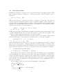
Operation
dist(a,l)
#a
a[i]
rep(d,v,i)
[s:e]
[s:e:d]
sum(a)
⊕ scan(a)
count(a)
permute(a,i)
Place elements a in d.
d <- a
a -> i
max index(a)
min index(a)
a ++ b
drop(a,n)
take(a,n)
rotate(a,n)
flatten(a)
partition(a,l)
split(a,f)
bottop(a)
Description
Distribute value a to sequence of length l.
Return length of sequence a.
Return element at position i of a.
Replace element at position i of d with v.
Return integer sequence from s to e.
Return integer sequence from s to e by d.
Return sum of sequence a.
Return scan based on operator ⊕.
Count number of true flags in a.
Permute elements of a to positions i.
L(a)
Write elements a in d.
Read from sequence a based on indices i.
Return index of the maximum value.
Return index of the minimum value.
Append sequences a and b.
Drop first n elements of sequence a.
Take first n elements of sequence a.
Rotate sequence a by n positions.
Flatten nested sequence a.
Partition sequence a into nested sequence.
Split a into nested sequence based on flags f.
Split a into nested sequence.
Work
S(result)
1
S(result)
S(v), S(v) + S(d)
(e - s)
(e - s)/d
S(a)
S(a)
S(a)
S(a)
1
S(a), S(a) + S(d)
S(result)
S(a)
S(a)
S(a) + S(b)
S(result)
S(result)
S(a)
S(a)
S(a)
S(a)
S(a)
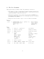
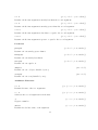
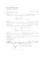
Table 1: List of some of the sequence functions supplied by Nesl. In the work column, S(v)
refers to the size of the object v. The * before certain functions means that those functions are
primitives. All the other functions can be built out of the primitives with at most a constant
factor overhead in both work and depth. For ⊕ scan the ⊕ can be one of {plus, max, min,
or, and}. All the sequence functions are described in detail in Appendix B.2. In rep and <-,
the work complexity depends on whether the variable used for d is the final reference to that
variable (arguments are evaluated left to right). If it is the final reference, then the complexity
before the comma is used, otherwise the complexity after the comma is used.
5
adds the two sequences elementwise. A full description of the apply-to-each construct is
given in Section 3.2.
In Nesl, any function, whether primitive or user defined, can be applied to each element
of a sequence. So, for example, we could define a factorial function
function factorial(i) =
if (i == 1) then 1
else i*factorial(i-1);
⇒
factorial : int -> int
and then apply it over the elements of a sequence
{factorial(x) :
⇒
x in [3,1,7]};
[6,1,5040] : [int]
In this example, the function name(arguments) = body; construct is used to define
factorial. The function is of type int -> int, indicating a function that maps integers to integers. The type is inferred by the compiler.
An apply-to-each construct applies a body to each element of a sequence. We will call
each such application an instance. Since there are no side effects in Nesl2 , there is no way
to communicate among the instances of an apply-to-each. An implementation can therefore
execute the instances in any order it chooses without changing the result. In particular,
the instances can be implemented in parallel, therefore giving the apply-to-each its parallel
semantics.
In addition to the apply-to-each construct, a second way to take advantage of parallelism
in Nesl is through a set of sequence functions. The sequence functions operate on whole
sequences and all have relatively simple parallel implementations. For example the function
sum sums the elements of a sequence.
sum([2, 1, -3, 11, 5]);
⇒
16 : int
Since addition is associative, this can be implemented on a parallel machine in logarithmic
time using a tree. Another common sequence function is the permute function, which
permutes a sequence based on a second sequence of indices. For example:
permute("nesl",[2,1,3,0]);
⇒
"lens" : [char]
In this case, the 4 characters of the string "nesl" (the term string is used to refer to a
sequence of characters) are permuted to the indices [2, 1, 3, 0] (n → 2, e → 1, s → 3,
and l → 0). The implementation of the permute function on a distributed-memory parallel
2
This is not strictly true since some of the utility functions, such as reading or writing from a file, have
side effects. These functions, however, cannot be used within an apply-to-each construct.
6
function kth smallest(s, k) =
let pivot = s[#s/2];
lesser = –e in s| e < pivot˝
in if (k < #lesser) then kth smallest(lesser, k)
else
let greater = –e in s| e > pivot˝
in if (k >= #s - #greater) then
kth smallest(greater, k - (#s - #greater))
else pivot;
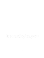
Figure 1: An implementation of order statistics. The function kth smallest returns the kth
smallest element from the input sequence s.
machine could use its communication network and the implementation on a shared-memory
machine could use an indirect write into the memory.
Table 1 lists some of the sequence functions available in Nesl. A subset of the functions
(the starred ones) form a complete set of primitives. These primitives, along with the
scalar operations and the apply-to-each construct, are sufficient for implementing the other
functions in the table with at most a constant factor increase in both the work and depth
complexities, as defined in Section 1.5. The table also lists the work complexity of each
function, which will also be defined in Section 1.5.
We now consider an example of the use of sequences in Nesl. The algorithm we consider
solves the problem of finding the kth smallest element in a set s, using a parallel version
of the quickorder algorithm [26]. Quickorder is similar to quicksort, but only calls itself
recursively on either the elements lesser or greater than the pivot. The Nesl code for
the algorithm is shown in Figure 1. The let construct is used to bind local variables (see
Section 3.2.2 for more details.). The code first binds len to the length of the input sequence
s, and then extracts the middle element of s as a pivot. The algorithm then selects all the
elements less than the pivot, and places them in a sequence that is bound to lesser. For
example:
s
pivot
{x in s | x < pivot}
=
=
=
[4, 8, 2, 3, 1, 7, 2]
3
[2, 1, 2]
After the pack, if the number of elements in the set lesser is greater than k, then the
kth smallest element must belong to that set. In this case, the algorithm calls kth smallest
recursively on lesser using the same k. Otherwise, the algorithm selects the elements that
are greater than the pivot, again using pack, and can similarly find if the kth element belongs
in the set greater. If it does belong in greater, the algorithm calls itself recursively, but
must now readjust k by subtracting off the number of elements lesser and equal to the
pivot. If the kth element belongs in neither lesser nor greater, then it must be the pivot,
and the algorithm returns this value.
7
1.2
Nested Parallelism
In Nesl the elements of a sequence can be any valid data item, including sequences. This
rule permits the nesting of sequences to an arbitrary depth. A nested sequence can be
written as
[[2, 1], [7,3,0], [4]]
This sequence has type: [[int]] (a sequence of sequences of integers). Given nested
sequences and the rule that any function can be applied in parallel over the elements of a
sequence, Nesl necessarily supplies the ability to apply a parallel function multiple times
in parallel; we call this ability nested parallelism. For example, we could apply the parallel
sequence function sum over a nested sequence:
{sum(v) :
⇒
v in [[2, 1], [7,3,0], [4]]};
[3, 10, 4] : [int]
In this expression there is parallelism both within each sum, since the sequence function has
a parallel implementation, and across the three instances of sum, since the apply-to-each
construct is defined such that all instances can run in parallel.
Nesl supplies a handful of functions for moving between levels of nesting. These include
flatten, which takes a nested sequence and flattens it by one level. For example,
flatten([[2, 1], [7, 3, 0], [4]]);
⇒
[2, 1, 7, 3, 0, 4] : [int]
Another useful function is bottop (for bottom and top), which takes a sequence of values
and creates a nested sequence of length 2 with all the elements from the bottom half of the
input sequence in the first element and elements from the top half in the second element (if
the length of the sequence is odd, the bottom part gets the extra element). For example,
bottop("nested parallelism");
⇒
["nested pa", "ralellism"] : [[char]]
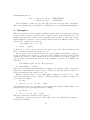
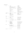
Table 2 lists several examples of routines that could take advantage of nested parallelism.
Nested parallelism also appears in most divide-and-conquer algorithms. A divide-andconquer algorithm breaks the original data into smaller parts, applies the same algorithm
on the subparts, and then merges the results. If the subproblems can be executed in parallel,
as is often the case, the application of the subparts involves nested parallelism. Table 3
lists several examples.
As an example, consider how the function sum might be implemented,
function my sum(a) =
if (#a == 1) then a[0]
else
let r = –my sum(v) : v in bottop(a)˝;
in r[0] + r[1];
8
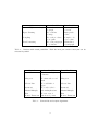
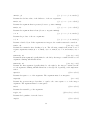
Application
Sum of Neighbors in Graph
Outer Parallelism
For each vertex
of graph
Inner Parallelism
Sum neighbors
of vertex
Figure Drawing
For each line
of image
Draw pixels
of line
Compiling
For each procedure
of program
Compile code
of procedure
Text Formatting
For each paragraph
of document
Justify lines
of paragraph
Table 2: Routines with nested parallelism. Both the inner part and the outer part can be
executed in parallel.
Algorithm
Quicksort
Outer Parallelism
For lesser and greater
elements
Inner Parallelism
Quicksort
Mergesort
For first and second
half
Mergesort
Closest Pair
For each half of
space
Closest Pair
Strassen’s
Matrix Multiply
For each of the 7
sub multiplications
Strassen’s
Matrix Multiply
Fast
Fourier Transform
For two sets of
interleaved points
Fast
Fourier Transform
Table 3: Some divide and conquer algorithms.
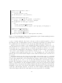
9
function qsort(a) =
if (#a < 2) then a
else
let pivot
= a[#a/2];
lesser = –e in a| e
equal
= –e in a| e
greater = –e in a| e
result = –qsort(v):
in result[0] ++ equal ++
< pivot˝;
== pivot˝;
> pivot˝;
v in [lesser,greater]˝
result[1];
Figure 2: An implementation of quicksort.
This code tests if the length of the input is one, and returns the single element if it is. If
the length is not one, it uses bottop to split the sequence in two parts, and then applies
itself recursively to each part in parallel. When the parallel calls return, the two results are
extracted and added.3 The code effectively creates a tree of parallel calls which has depth
lg n, where n is the length of a, and executes a total of n − 1 calls to +.
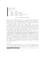
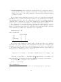
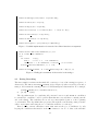
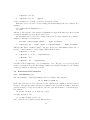
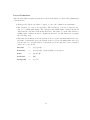
As another more involved example, consider a parallel variation of quicksort [6] (see
Figure 2). When applied to a sequence s, this version splits the values into three subsets (the
elements lesser, equal and greater than the pivot) and calls itself recursively on the lesser
and greater subsets. To execute the two recursive calls, the lesser and greater sequences
are concatenated into a nested sequence and qsort is applied over the two elements of the
nested sequences in parallel. The final line extracts the two results of the recursive calls
and appends them together with the equal elements in the correct order.
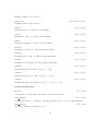
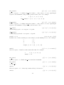
The recursive invocation of qsort generates a tree of calls that looks something like the
tree shown in Figure 3. In this diagram, taking advantage of parallelism within each block
as well as across the blocks is critical to getting a fast parallel algorithm. If we were only
to take advantage of the parallelism within each quicksort to subselect the two sets (the
parallelism within each block), we would do well near the root and badly near the leaves
(there are n leaves which would be processed serially). Conversely, if we were only to take
advantage of the parallelism available by running the invocations of quicksort in parallel
(the parallelism between blocks but not within a block), we would do well at the leaves
and badly at the root (it would take n time to process the root). In both cases the parallel
time complexity is O(n) rather than the ideal O(lg2 n) we can get using both forms (this
is discussed in Section 1.5).
1.3
Pairs
As well as sequences, Nesl supports the notion of pairs. A pair is a structure with two
elements, each of which can be of any type. Pairs are often used to build simple structures
or to return multiple values from a function. The binary comma operator is used to create
3
To simulate the built-in sum, it would be necessary to add code to return the identity (0) for empty
sequences.
10
Quicksort
↓
Quicksort
↓
Quicksort
↓
↓
Qs
Qs
↓
Quicksort
↓
Quicksort
↓
Quicksort
↓
↓
Qs
Qs
↓
Qs
↓
Quicksort
↓
↓
Qs
Qs
↓
Quicksort
↓
↓
Quicksort
Qs
↓
↓
Qs
Qs
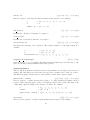
Figure 3: The quicksort algorithm. Just using parallelism within each block yields a parallel
running time at least as great as the number of blocks (O(n)). Just using parallelism from
running the blocks in parallel yields a parallel running time at least as great as the largest block
(O(n)). By using both forms of parallelism the parallel running time can be reduced to the
depth of the tree (expected O(lg n)).
pairs. For example:
9.8,"foo";
⇒
(9.8,"foo") : (float, [char])
2,3;
⇒
(2,3) : (int, int)
The comma operator is right associative (e.g. (2,3,4,5) is equivalent to (2,(3,(4,5)))).
All other binary operators in Nesl are left associative. The precedence of the comma
operator is lower than any other binary operator, so it is usually necessary to put pairs
within parentheses.
Pattern matching inside of a let construct can be used to deconstruct structures of
pairs. For example:
let (a,b,c) = (2*4,5-2,4)
in a+b*c;
⇒
20 : int
In this example, a is bound to 8, b is bound to 3, and c is bound to 4.
Nested pairs differ from sequences in several important ways. Most importantly, there
is no way to operate over the elements of a nested pair in parallel. A second important
difference is that the elements of a pair need not be of the same type, while elements of a
sequence must always be of the same type.
11
1.4
Types
Nesl is a strongly typed polymorphic language with a type inference system. Its type
system is similar to functional languages such as ML, but since it is first-order (functions
cannot be passed as data), function types only appear at the top level. As well as parametric
polymorphism Nesl also allows a form of overloading similar to what is supplied by the
Haskell Language [28].
The type of a polymorphic function in Nesl is specified by using type-variables, which
are declared in a type-context. For example, the type of the permute function is:
([A], [int]) -> [A] ::
A in any
This specifies that for A bound to any type, permute maps a sequence of type [A] and a
sequence of type [int] into another sequence of type [A]. The variable A is a type-variable,
and the specification A in any is the context. A context can have multiple type bindings
separated by semicolons. For example, the zip function, which zips two sequences of equal
length together into one sequence of pairs, has type:
([A], [B]) -> [(A,B)] ::
A in any; B in any
User defined functions can also be polymorphic. For example we could define
function append3(s1,s2,s3) = s1 ++ s2 ++ s3;
⇒
append3(s1,s2,s3) : ([A], [A], [A]) -> [A] ::
A in any
The type inference system will always determine the most general type possible.
In addition to parametric polymorphism, Nesl supports a form of overloading by including the notion of type-classes. A type-class is a set of types along with an associated
set of functions. The functions of a class can only be applied to the types from that class.
For example the base types, int and float are both members of the type class number,
and numerical functions such as + and * are defined to work on all numbers. The type of
a function overloaded in this way, is specified by limiting the context of a type-variable to
a specific type-class. For example, the type of + is:
(A, A) -> A ::
A in number
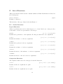
The context “A in number” specifies that A can be bound to any member of the typeclass number. The fully polymorphic specification any can be thought of as type-class that
contains all data types as members. The type-classes are organized into the hierarchy as
shown in Figure 4. Functions such as = and < are defined on ordinals, functions such as +
and * are defined on numbers, and functions such as or and not are defined on logicals.
User-defined functions can also be overloaded. For example:
function double(a) = a + a;
⇒
double(a) :
A -> A ::
A in number
It is also possible to restrict the type of a user-defined function by explicitly typing it. For
example,
12
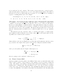
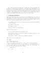
any
|
\
ordinal
|
ALL OTHER DATA TYPES
/
\
\
/
number logical
/
/
\ /
|
CHAR FLOAT INT BOOL
/
Figure 4: The type-class hierarchy of Nesl. The lower case names are the type classes.
function double(a) :
⇒
int -> int = a + a;
double(a) : int -> int
limits the type of double to int -> int. The : specifies that the next form is a typespecifier (see Appendix A for the full syntax of the function construct and type specifiers).
In certain situations the type inference system cannot determine the type even though
there is one. For example the function:
function badfunc(a,b) = a or (a + b);
will not type properly because or is defined on the type-class logical and + is defined on
the type-class number. As it so happens, int is both a logical and an integer, but the Nesl
inference system does not know how to take intersections of type-classes. In this situation
it is necessary to specify the type:
function goodfunc(a,b) :
⇒
int, int -> int = a or (a + b);
goodfunc(a,b) : int, int -> int
This situation comes up quite rarely.
Specifying the type using “:” serves as good documentation for a function even when
the inference system can determine the type. The notion of type-classes in Nesl is similar
to the type-classes used in the Haskell language [28], but, unlike Haskell, Nesl currently
does not permit the user to add new type classes.4
1.5
Deriving Complexity
There are two complexities associated with all computations in Nesl.
1. Work complexity: this represents the total work done by the computation, that is
to say, the amount of time that the computation would take if executed on a serial
random access machine. The work complexity for most of the sequence functions is
simply the size of one of its arguments. A complete list is given in Table 1. The size
of an object is defined recursively: the size of a scalar value is 1, and the size of a
sequence is the sum of the sizes of its elements plus 1.
4
It is likely that future versions of Nesl will allow such extensions.
13
2. Depth complexity: this represents the parallel depth of the computation, that is to
say, the amount of time the computation would take on a machine with an unbounded
number of processors. The depth complexity of all the sequence functions supplied
by Nesl is constant.
The work and depth complexities are based on the vector random access machine
(VRAM) model [7], a strictly data-parallel abstraction of the parallel random access machine (PRAM) model [19]. Since the complexities are meant for determining asymptotic
complexity, these complexities do not include constant factors. All the Nesl functions,
however, can be executed in a small number of machine instructions per element.
The complexities are combined using simple combining rules. Expressions are combined
in the standard way—for both the work complexity and the depth complexity, the complexity of an expression is the sum of the complexities of the arguments plus the complexity
of the call itself. For example, the complexities of the computation:
sum(dist(7,n)) * #a
can be calculated as:
dist
sum
# (length)
*
Total
Work
n
n
1
1
O(n)
Depth
1
1
1
1
O(1)
The apply-to-each construct is combined in the following way. The work complexity
is the sum of the work complexity of the instantiations, and the depth complexity is the
maximum over the depth complexities of the instantiations. If we denote the work required
by an expression exp applied to some data a as W (exp(a)), and the depth required as
D(exp(a)), these combining rules can be written as
W ({e1(a) : a in e2(b)}) = W (e2(b)) + sum({W (e1(a)) : a in e2(b)})
(1)
D({e1(a) : a in e2(b)}) = D(e2(b)) + max val({D(e1(a)) : a in e2(b)}) (2)
where sum and max val just take the sum and maximum of a sequence, respectively.5
As an example, the complexities of the computation:
{[0:i] :
i in [0:n]}
can be calculated as:
5
For comments about how these equations relate to the current implementation see Appendix C.
14
Work
[0:n]
n
Parallel Calls
Pi<n
[0:i]
i=0 i
Total
O(n2 )
Depth
1
maxi<n
i=0 1
O(1)
Once the work (W ) and depth (D) complexities have been calculated in this way, the
formula
T
= O(W/P + D lg P )
(3)
places an upper bound on the asymptotic running time of an algorithm on the CRCW
PRAM model (P is the number of processors). This formula can be derived from Brent’s
scheduling principle [14] as shown in [41, 7, 30]. The lg P term shows up because of the
cost of allocating tasks to processors, and the cost of implementing the sum and scan
operations. On the scan-PRAM [6], where it is assumed that the scan operations are no
more expensive than references to the shared-memory (they both require O(lg P ) on a
machine with bounded degree circuits), then the equation is:
T
= O(W/P + D)
(4)
In the mapping onto a PRAM, the only reason a concurrent-write capability is required is
for implementing the <- (write) function, and the only reason a concurrent-read capability is
required is for implementing the -> (read) function. Both of these functions allow repeated
indices (“collisions”) and could therefore require concurrent access to a memory location.
If an algorithm does not use these functions, or guarantees that there are no collisions
when they are used, then the mapping can be implemented with a EREW PRAM. Out of
the algorithms in this paper, the primes algorithm (Section 2.2) requires concurrent writes,
and the string-searching algorithm (Section 2.1) requires concurrent reads. All the other
algorithms can use an EREW PRAM.
As an example of how the work and depth complexities can be used, consider the
kth smallest algorithm described earlier (Figure 1). In this algorithm the work is the
same as the time required by the standard serial version (loops have been replaced by
parallel calls), which has an expected time of O(n) [18]. It is also not hard to show that
the expected number of recursive calls is O(lg n), since we expect to drop some fraction of
the elements on each recursive call [37]. Since each recursive call requires a constant depth,
we therefore have:
W (n) = O(n)
D(n) = O(lg n)
Using Equation 3 this gives us an expected case running time on a PRAM of:
T (n) = O(n/p + lg n lg p) = O(n/p + lg2 n)
= O(n/p + lg n)
EREW PRAM
scan-PRAM
One can similarly show for the quicksort algorithm given in Figure 2 that the work and
depth complexities are W (n) = O(n lg n) and D(n) = O(lg n) [37], which give a EREW
15
PRAM running time of:
T (n) = O(n lg n/p + lg2 n)
= O(n lg n/p + lg n)
EREW PRAM
scan-PRAM
In the remainder of this paper we will only derive the work and depth complexities.
The reader can plug these into Equation 3 or Equation 4 to get the PRAM running times.
2
Examples
This section describes several examples of Nesl programs. Before describing the examples
we describe three common operations. The -> binary operator (called read) is used to read
multiple elements from a sequence. Its left argument is the sequence to read from, and the
right argument is a sequence of integer indices which specify from which locations to read
elements. For example, the expression
"an example"->[7, 0, 8, 4];
⇒
"pale" : [char]
reads the p, a, l and e from locations 7, 0, 8 and 4, respectively. The read function can
also be expressed as read(a,i) instead of a -> i.
The <- binary operator (called write) is used to write multiple elements into a sequence.
Its left argument is the sequence to write into (the destination sequence) and its right
argument is a sequence of integer-value pairs. For each element (i,v) in the sequence of
pairs, the value v is written at position i of the destination sequence. For example, the
expression
"an example"<-[(4,‘s),(2,‘d),(3,space)];
⇒
"and sample" : [char]
writes the s, d and space into the string "an example" at locations 4, 2 and 3, respectively
(space is a constant that is bound to the space character). The write function can also be
expressed as write(d,iv) instead of d <- iv.
Ranges of integers can be created using square brackets along with a colon.
The
notation [start:end] creates a sequence of integers starting at start and ending one
before end. For example:
[10:16];
⇒
[10, 11, 12, 13, 14, 15] : [int]
An additional stride can be specified, as in [start:end:stride], which returns every
strideth integer between start and end. For example:
[10:25:3];
⇒
[10, 13, 16, 19, 22] : [int]
The integer end is never included in the sequence.
Using these operations, it is easy to define many of the other Nesl functions. Figure 5
shows several examples.
16
function subseq(a,start,end) = a->[start:end];
function take(a,n) = a->[0:n];
function drop(a,n) = a->[n:#a];
function rotate(a,n) = a->–mod(i-n,#a) :
i in [n:n + #a]˝;
function even elts(a) = a->[0:#a:2];
function odd elts(a) = a->[1:#a:2];
function bottop(a) = [a->[0:#a/2],a->[#a/2:#a]];
Figure 5: Possible implementation for several of the Nesl functions on sequences.
function next character(candidates,w,s,i) =
if (i == #w) then candidates
else
let letter
= w[i];
next l
= s->–c + i: c in candidates˝;
candidates = –c in candidates; n in next l | n == letter˝
in next character(candidates, w, s, i+1);
function string search(w, s) = next character([0:#s - #w],w,s,0);
Figure 6: Finding all occurrences of the word w in the string s.
2.1
String Searching
The first example is a function that finds all occurrences of a word in a string (a sequence of
characters). The function string search(w,s) (see Figure 6) takes a search word w and a
string s, and returns the starting position of all substrings in s that match w. For example,
string search("foo","fobarfoofboofoo");
⇒
[5,12] : [int]
The algorithm starts by considering all positions between 0 and #s-#w as candidates
for a match (no candidate could be greater than this since it would have to match past the
end of the string). The candidates are stored as pointers (indices) into s of the beginning
of each match. The algorithm then progresses through the search string, using recursive
calls to next char, narrowing the set of candidate matches on each step.
Based on the current candidates, next char narrows the set of candidates by only
keeping the candidates that match on the next character of w. To do this, each candidate
17
function primes(n) =
if n == 2 then [2]
else
let sqr primes = primes(ceil(sqrt(float(n))));
sieves = –[2*p:n:p]: p in sqr primes˝;
flat sieves = flatten(sieves);
flags = dist(t,n) <- –(i,f): i in flat sieves˝
in drop(–i in [0:n]; flag in flags| flag˝, 2) ;
Figure 7: Finding all the primes less than n.
checks whether the ith character in w matches the ith position past the candidate index.
All candidates that do match are packed and passed into the recursive call of next char.
The recursion completes when the algorithm reaches the end of w. The progression of
candidates in the "foo" example would be:
i
0
1
2
candidates
[0, 5, 8, 12]
[0, 5, 12]
[5, 12]
Lets consider the complexity of the algorithm. We assume #w = m and #s = n. The
depth complexity of the algorithm is some constant times the number of recursive calls,
which is simply O(m). The work complexity of the algorithm is the sum over the recursive
calls, of the number of candidates in each recursive call. In practice, this is usually O(n),
but in the worst case this can be the product of the two lengths O(nm) (the worst case can
only happen if most of the characters in w are repeated). There are parallel string-searching
algorithms that give better bounds on the parallel time (depth complexity), and that bound
the worst case work complexity to be linear in the length of the search string [15, 44], but
these algorithms are somewhat more complicated.
2.2
Primes
Our second example finds all the primes less than n. The algorithm is based on the sieve
√
of Eratosthenes. The basic idea of the sieve is to find all the primes less than n, and then
use multiples of these primes to “sieve out” all the composite numbers less than n. Since
√
all composite numbers less than n must have a divisor less than n, the only elements left
unsieved will be the primes. There are many parallel versions of the prime sieve, and several
naive versions require a total of O(n3/2 ) work and either O(n1/2 ) or O(n) parallel time. A
well designed version should require no more work than the serial sieve (O(n lg lg n)), and
polylogarithmic parallel time.
The version we use (see Figure 7) requires O(n lg lg n) work and O(lg lg n) depth. It
√
works by first recursively finding all the primes up to n, (sqr primes). Then, for each
prime p in sqr primes, the algorithm generates all the multiples of p up to n (sieves). This
18
is done with the [s:e:d] construct. The sequence sieves is therefore a nested sequence
with each subsequence being the sieve for one of the primes in sqr primes. The function
flatten, is now used to flatten this nested sequence by one level, therefore returning a
sequence containing all the sieves. For example,
flatten([[4, 6, 8, 10, 12, 14, 16, 18], [6, 9, 12, 15, 18]]);
⇒
[4, 6, 8, 10, 12, 14, 16, 18, 6, 9, 12, 15, 18] : [int]
This sequence of sieves is used by the <- function to place a false flag in all positions that
are a multiple of one of the sqr primes. This will return a boolean sequence, flags, which
contains a t in all places that were not knocked out by a sieve—these are the primes.
However, we want primes to return the indices of the primes instead of flags. To generate
these indices the algorithm creates a sequences of all indices between 0 and n ([0:n]) and
uses subselection to remove the nonprimes. The function drop is then used to remove the
first two elements (0 and 1), which are not considered primes but do not get explicitly
sieved.
The functions [s:e:d], flatten, dist, <- and drop all require a constant depth.
√
Since primes is called recursively on a problem of size n the total depth required by the
algorithm can be written as the recurrence:
(
D(n) =
O(1)
n=1
√
D( n) + O(1) n > 1
= O(lg lg n)
Almost all the work done by primes is done in the first call. In this first call, the work is
proportional to the length of the sequence flat sieves. Using the standard formula
X
1/p = log log x + C + O(1/ log x)
p≤x
where p are the primes [24], the length of this sequence is:
X
√
n/p = O(n log log n)
√
p≤ n
= O(n log log n)
therefore giving a work complexity of O(n log log n).
2.3
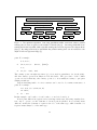
Planar Convex-Hull
Our next example solves the planar convex hull problem: given n points in the plane, find
which of these points lie on the perimeter of the smallest convex region that contains all
points. The planar convex hull problem has many applications ranging from computer
graphics [21] to statistics [27]. The algorithm we use to solve the problem is a parallel
version [12] of the quickhull algorithm [36]. The quickhull algorithm was given its name
because of its similarity to the quicksort algorithm. As with quicksort, the algorithm picks
19
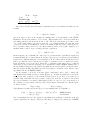
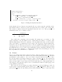
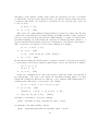
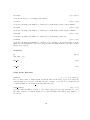
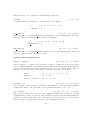
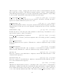
Figure 8: An example of the quickhull algorithm. Each sequence shows one step of the
algorithm. Since A and P are the two x extrema, the line AP is the original split line. J and
N are the farthest points in each subspace from AP and are, therefore, used for the next level
of splits. The values outside the brackets are hull points that have already been found.
20
function cross product(o,line) =
let (xo,yo) = o;
((x1,y1),(x2,y2)) = line
in (x1-xo)*(y2-yo) - (y1-yo)*(x2-xo);
function hsplit(points,p1,p2) =
let cross = –cross product(p,(p1,p2)): p in points˝;
packed = –p in points; c in cross | plusp(c)˝
in if (#packed < 2) then [p1] ++ packed
else
let pm = points[max index(cross)]
in flatten(–hsplit(packed,p1,p2): p1 in [p1,pm]; p2 in [pm,p2]˝);
function convex hull(points) =
let x = –x : (x,y) in points˝;
minx = points[min index(x)];
maxx = points[max index(x)]
in hsplit(points,minx,maxx) ++ hsplit(points,maxx,minx);
Figure 9: Code for Quickhull. Each point is represented as a pair. Pattern matching is used to
extract the x and y coordinates of each pair.
a “pivot” element, splits the data based on the pivot, and is recursively applied to each of
the split sets. Also, as with quicksort, the pivot element is not guaranteed to split the data
into equally sized sets, and in the worst case the algorithm will require O(n2 ) work.
Figure 8 shows an example of the quickhull algorithm, and Figure 9 shows the code.
The algorithm is based on the recursive routine hsplit. This function takes a set of points
in the plane (hx, yi coordinates) and two points p1 and p2 that are known to lie on the
convex hull, and returns all the points that lie on the hull clockwise from p1 to p2, inclusive
of p1, but not of p2. In Figure 8, given all the points [A, B, C, ..., P], p1 = A and p2
= P, hsplit would return the sequence [A, B, J, O]. In hsplit, the order of p1 and p2
matters, since if we switch A and P, hsplit would return the hull along the other direction
[P, N, C].
The hsplit function works by first removing all the elements that cannot be on the hull
since they lie below the line between p1 and p2. This is done by removing elements whose
cross product with the line between p1 and p2 are negative. In the case p1 = A and p2 =
P, the points [B, D, F, G, H, J, K, M, O] would remain and be placed in the sequence
packed. The algorithm now finds the point furthest from the line p1-p2. This point pm
must be on the hull since as a line at infinity parallel to p1-p2 moves toward p1-p2, it must
first hit pm. The point pm (J in the running example) is found by taking the point with the
maximum cross-product. Once pm is found, hsplit calls itself twice recursively using the
points (p1, pm) and (pm, p2) ((A, J) and (J, P) in the example). When the recursive
calls return, hsplit flattens the result (this effectively appends the two subhulls).
21
The overall convex-hull algorithm works by finding the points with minimum and
maximum x coordinates (these points must be on the hull) and then using hsplit to find
the upper and lower hull. Each recursive call has a depth complexity of O(1) and a work
complexity of O(n). However, since many points might be deleted on each step, the work
complexity could be significantly less. For m hull points, the algorithm runs in O(lg m)
depth for well-distributed hull points, and has a worst case depth of O(m).
3
Language Definition
This section defines Nesl. It is not meant as a formal semantics but, along with the
full definition of the syntax in Appendix A and description of all the built-in functions in
Appendix B, it should serve as an adequate description of the language. Nesl is a strict
first-order strongly-typed language with the following data types:
• four primitive atomic data types: booleans (bool), integers (int), characters (char),
and floats (float);
• the primitive sequence type;
• the primitive pair type;
• and user definable compound datatypes;
and the following operations:
• a set of predefined functions on the primitive types;
• three primitive constructs: a conditional construct if, a binding construct let, and
the apply-to-each construct;
• and a function constructor, function, for defining new functions.
This section covers each of these topics.
3.1
3.1.1
Data
Atomic Data Types
There are four primitive atomic data types: booleans, integers, characters and floats.
The boolean type bool can have one of two values t or f. The standard logical operations (eg. not, and, or, xor, nor, nand) are predefined. The operations and, or,
xor, nor, nand all use infix notation. For example:
not(not(t));
⇒
t : bool
22
t xor f;
⇒
t : bool
The integer type int is the set of (positive and negative) integers that can be represented
in the fixed precision of a machine-sized word. The exact precision is machine dependent,
but will always be at least 32-bits. The standard functions on integers (+, -, *, /,
==, >, <, negate, ...) are predefined, and use infix notation (see Appendix A for the
precedence rules). For example:
3 * -11;
⇒
-33 : int
7 == 8;
⇒
f : bool
Overflow will return unpredictable results.
The character type char is the set of ASCII characters. The characters have a fixed
order and all the comparison operations (eg. ==, <, >=,...) can be used. Characters are
written by placing a ‘ in front of the character. For example:
‘8;
⇒
‘8 : char
‘a == ‘d;
⇒
f : bool
‘a < ‘d;
⇒
t : bool
The global variables space, newline and tab are bound to the appropriate characters.
The type float is used to specify floating-point numbers. The exact representation of
these numbers is machine specific, but Nesl tries to use 64-bit IEEE when possible. Floats
support most of the same functions as integers, and also have several additional functions
(eg. round, truncate, sqrt, log,...). Floats must be written by placing a decimal
point in them so that they can be distinguished from integers.
1.2 * 3.0;
⇒
3.6 : float
round(2.1);
⇒
2 : int
There is no implicit coercion between scalar types. To add 2 and 3.0, for example, it is
necessary to coerce one of them: e.g.
float(2) + 3.0;
⇒ 5.0 : float
A complete list of the functions available on scalar types can be found in Appendix B.1.
23
3.1.2
Sequences ([])
A sequence can contain any type, including other sequences, but each element in a sequence
must be of the same type (sequences are homogeneous). The type of a sequence whose
elements are of type α, is specified as [α]. For examples:
[6, 2, 4, 5];
⇒
[6, 2, 4, 5] : [int]
[[2, 1, 7, 3], [6, 2], [22, 9]];
⇒
[[2, 1, 7, 3], [6, 2], [22, 9]] : [[int]]
Sequences of characters can be written between double quotes,
"a string";
⇒
"a string" : [char]
but can also be written as a sequence of characters:
[‘a, Space, ‘s, ‘t, ‘r, ‘i, ‘n, ‘g];
⇒
"a string" : [char]
Empty sequences must be explicitly typed since the type cannot be determined from
the elements. The type of an empty sequences is specified by using empty square braces
followed by the type of the elements. For example,
[] int;
⇒
[] : [int]
[] (int,bool);
⇒
[] : [(int,bool)]
Appendix B.2 describes the functions that operate on sequences.
3.1.3
Record Types (datatype)
Record types with a fixed number of slots can be defined with the datatype construct. For
example,
datatype complex(float,float);
⇒
complex(a1,a2) : float, float -> complex
defines a record with two slots both which must contain a floating-point number. Defining
a record also defines a corresponding function that is used to construct the record. For
example,
24
complex(7.1,11.9);
⇒
complex(7.1,11.9) : complex
creates a complex record with 7.1 and 11.9 as its two values.
Elements of a record can be accessed using pattern matching in the let construct. For
example,
let complex(real,imaginary) = a
in real;
will remove the real part of the variable a (assuming it is kept in the first slot). More details
on pattern matching are given in the next section.
As with functions, records can be parameterized based on type-variables. For example,
complex could have been defined as:
datatype complex(alpha,alpha) ::
⇒
alpha in number;
complex(a1,a2) : alpha, alpha -> complex(alpha) ::
alpha in number
This specifies that for alpha bound to any type in the type-class number (either int or
float), both slots must be of type alpha. This will allow either,
complex(7.1, 11.9);
⇒
complex(7.1, 11.9) : complex(float)
complex(7, 11);
⇒
complex(7, 11) : complex(int)
but will not allow complex(7, ‘a) or complex(2, 2.2). The type of a record is specified
by the record name followed by the binding of all its type-variables. In this case, the binding
of the type-variable is either int or float.
3.2
Functions and Constructs
3.2.1
Conditionals (if)
The only primitive conditional in Nesl is the if construct. The syntax is:
IF exp THEN exp ELSE exp
If the first expression is true, then the second expression is evaluated and its result is
returned, otherwise the third expression is evaluated and its result is returned. The first
expression must be of type bool, and the other two expressions must be of identical types.
For example:
if (t and f) then 3 + 4 else (6 - 2)*7
is a valid expression, but
if (t and f) then 3 else 2.6
is not, since the two branches return different types.
25
3.2.2
Binding Local Variables (let)
Local variables can be bound with the let construct. The syntax is:
LET expbinds IN exp
expbinds
::=
expbind [; expbinds]
variable bindings
expbind
::=
pattern = exp
variable binding
pattern
::=
ident
ident(pattern)
pattern, pattern
( pattern )
variable
datatype pattern
pair pattern
The semicolon separates bindings (the square brackets indicate an optional term of the
syntax). Each pattern is either a variable name or a pattern based on a record name. Each
expbind binds the variables in the pattern on the left of the = to the result of the expression
on the right. For example:
let a = 7;
(b,c) = (1,2)
in a*(b + c);
⇒
21 : int
Here a is bound to 7, then the pattern (b, c) is matched with the result of the expression
on the right so that b is bound to 1 and c is bound to 2. Patterns can be nested, and the
patterns are matched recursively.
The variables in each expbind can be used in the expressions (exp) of any later expbind
(the bindings are done serially). For example, in the expression
let a = 7;
b = a + 4
in a * b;
⇒
77 : int
the variable a is bound to the value 7 and then the variable b is bound to the value of a
plus 4, which is 11. When these are multiplied in the body, the result is 77.
3.2.3
The Apply-to-Each Construct ({})
The apply-to-each construct is used to apply any function over the elements of a sequence.
It has the following syntax:
{[exp :]
rbinds [| exp]}
rbinds
::=
rbind [; rbinds]
rbind
::=
pattern IN exp
ident
full binding
shorthand binding
26
An apply-to-each construct consists of three parts: the expression before the colon, which
we will call the body, the bindings that follow the body, and the expression that follows the
|, which we will call the sieve. Both the body and the sieve are optional: they could both
be left out, as in
{a in [1, 2, 3]};
⇒
[1, 2, 3] : [int]
The rbinds can contain multiple bindings which are separated by semicolons. We first
consider the case in which there is a single binding. A binding can either consist of a pattern
followed by the keyword IN and an expression (full binding), or consist of a variable name
(shorthand binding). In a full binding the expression is evaluated (it must evaluate to a
sequence) and the variables in the pattern are bound in turn to each element of the sequence.
The body and sieve are applied for each of these bindings. For example:
{a + 2:
⇒
[3, 4, 5] : [int]
{a + b:
⇒
a in [1, 2, 3]};
(a,b) in [(1,2), (3,4), (5,6)]};
[3, 7, 11] : [int]
In a shorthand binding, the variable must be a sequence, and the body and sieve are applied
to each element of the sequence with the variable name bound to the element. For example:
let a = [1, 2, 3]
in {a + 2: a};
⇒
[3, 4, 5] : [int]
In the case of multiple rbinds, each of the sequences (either the result of the expression
in a full binding or the value of the variable in a shorthand binding) must be of equal
length. The bindings are interleaved so that the body is evaluated with bindings made for
elements at the same index of each sequence. For example:
{a + b:
⇒
a in [1, 2, 3]; b in [1, 4, 9]};
[2, 6, 12] : [int]
{dist(b,a):
⇒
a in [1, 2, 3]; b in [1, 4, 9]};
[[1], [4, 4], [9, 9, 9]] : [[int]]
An apply-to-each with a body and two bindings,
{body:
pattern1 in exp1; pattern2 in exp2 | sieve}
is equivalent to the single binding construct
{body:
(pattern1,pattern2) in zip(exp1,exp2) | sieve}
27
where zip, as defined in the list of functions, elementwise zips together the two sequences
it is given as arguments.
If there is no body in an apply-to-each construct, then the results of the first binding is
returned. For example:
{a in [1, 2, 3]; b in [1, 4, 9]};
⇒
[1, 2, 3] : [int]
{a in [1, 2, 3]; b in [2, 4, 9] | b == 2*a};
⇒
[1, 2] : [int]
{b in [2, 4, 9]; a in [1, 2, 3] | b == 2*a};
⇒
[2, 4] : [int]
If there is a body and a sieve, the body and sieve are both evaluated for all bindings,
and then the subselection is applied. An apply-to-each with a sieve of the form:
{body :
bindings | sieve}
is equivalent to the construct
pack({(body,sieve) :
bindings})
where pack, as defined in the list of functions, takes a sequence of type [(alpha,bool)]
and returns a sequence which contains the first element of each pair if the second element
is true. The order of remaining elements is maintained.
3.2.4
Defining New Functions (function)
Functions can be defined at top-level using the function construct. The syntax is:
FUNCTION ident pattern [:
funtype] = exp ;
A function has one argument, but the argument can be any pattern. The body of a
function (the exp at the end) can only refer to variables bound in the pattern, or variables
declared at top-level. Any function referred to in the body can only refer to functions
previously defined or to the function itself (at present there is no way to define mutually
recursive functions). As with all functional languages, defining a function with the same
name as a previous function only hides the previous function from future use: all references
to a function before the new definition will refer to the original definition.
3.2.5
Top-Level Bindings (=)
You can bind a variable at top-level using the = operator. The syntax is:
ident = exp;
28
For example, a = 211; will bind the variable a to the value 211. The variable can now
either be referenced at top level, or can be referenced inside of any function. For example,
the definition
function foo(c) = c + a;
would define a function that adds 211 to its input. Such top-level binding is mostly useful
for saving temporary results at top-level, and for defining constants. The variable pi is
bound at top level to the value of π.
Acknowledgments
I would like to thank Marco Zagha, Jay Sipelstein, Margaret Reid-Miller, Bob Harper,
Jonathan Hardwick, John Greiner, Tim Freeman, and Siddhartha Chatterjee for many
helpful comments on this manual. Siddhartha Chatterjee, Jonathan Hardwick, Jay Sipelstein, and Marco Zagha did all the work getting the intermediate languages VCODE and
CVL running so that NESL can actually run on parallel machines. Dafna Talmor and Yury
Smirnov helped with the X plotting code.
References
[1] ANSI. ANSI Fortran Draft S8, Version 111.
[2] Andrew W. Appel and David B. MacQueen. Standard ML of New Jersey. In Martin
Wirsing, editor, Third Int’l Symp. on Prog. Lang. Implementation and Logic Programming, New York, August 1991. Springer-Verlag.
[3] Arvind, Rishiyur S. Nikhil, and Keshav K. Pingali. I-structures: Data structures
for parallel computing. ACM Transactions on Programming Languages and Systems,
11(4):598–632, October 1989.
[4] G. Blelloch, G.L. Miller, and D. Talmor. Parallel Delaunay triangulation implementation. In MSI workshop on Computational geometry, Cornell, Oct 1994.
[5] Guy Blelloch and Girija Narlikar. A comparison of two n-body algorithms. In Dimacs
implementation challenge workshop, October 1994.
[6] Guy E. Blelloch. Scans as primitive parallel operations. IEEE Transactions on Computers, C-38(11):1526–1538, November 1989.
[7] Guy E. Blelloch. Vector Models for Data-Parallel Computing. MIT Press, 1990.
[8] Guy E. Blelloch, Siddhartha Chatterjee, Jonathan C. Hardwick, Jay Sipelstein, and
Marco Zagha. Implementation of a portable nested data-parallel language. Journal of
Parallel and Distributed Computing, 21(1):4–14, April 1994.
29
[9] Guy E. Blelloch, Siddhartha Chatterjee, Fritz Knabe, Jay Sipelstein, and Marco Zagha.
VCODE reference manual (version 1.1). Technical Report CMU-CS-90-146, School of
Computer Science, Carnegie Mellon University, July 1990.
[10] Guy E. Blelloch and Jonathan C. Hardwick. Class notes: Programming parallel algorithms. Technical Report CMU-CS-93-115, School of Computer Science, Carnegie
Mellon University, February 1993.
[11] Guy E. Blelloch, Jonathan C. Hardwick, Jay Sipelstein, and Marco Zagha. NESL
user’s manual (for NESL version 3.1). Technical Report CMU-CS-95-169, Carnegie
Mellon University, July 1995.
[12] Guy E. Blelloch and James J. Little. Parallel solutions to geometric problems on
the scan model of computation. In Proceedings International Conference on Parallel
Processing, pages Vol 3: 218–222, August 1988.
[13] Guy E. Blelloch and Gary W. Sabot. Compiling collection-oriented languages onto
massively parallel computers. Journal of Parallel and Distributed Computing, 8(2):119–
134, February 1990.
[14] Richard P. Brent. The parallel evaluation of general arithmetic expressions. Journal
of the Association for Computing Machinery, 21(2):201–206, 1974.
[15] D. Breslauer and Z. Galil. An optimal O(log log n) time parallel string matching
algorithm. SIAM Journal on Computing, 19(6):1051–1058, December 1990.
[16] Siddhartha Chatterjee. Compiling Data-Parallel Programs for Efficient Execution on
Shared-Memory Multiprocessors. PhD thesis, School of Computer Science, Carnegie
Mellon University, October 1991.
[17] Siddhartha Chatterjee, Guy E. Blelloch, and Marco Zagha. Scan primitives for vector
computers. In Proceedings Supercomputing ’90, pages 666–675, November 1990.
[18] T. H. Cormen, C. E. Leiserson, and R. L. Rivest. Introduction to Algorithms. The
MIT Press and McGraw-Hill, 1990.
[19] Steven Fortune and James Wyllie. Parallelism in random access machines. In Proceedings ACM Symposium on Theory of Computing, pages 114–118, 1978.
[20] Message Passing Interface Forum. Draft document for a standard message-passing
interface. Technical Report CS-93-214, University of Tennessee, November 1993.
[21] H. Freeman. Computer processing of line-drawing images. Computer Surveys, 6:57–97,
1974.
[22] John Greiner. A comparison of data-parallel algorithms for connected components. In
Proceedings Sixth Annual Symposium on Parallel Algorithms and Architectures, pages
16–25, Cape May, NJ, June 1994.
30
[23] John Greiner and Guy E. Blelloch. The NESL cost semantics. In preparation, 1995.
[24] G. H. Hardey and E. M. Wright. An Introduction to the Theory of Numbers, 5th ed.
Oxford University Press, Oxford, New York, 1983.
[25] Jonathan C. Hardwick. Porting a vector library: a comparison of MPI, Paris, CMMD
and PVM. In Scalable Parallel Libraries Conference, pages 68–77, Starkville, Mississippi, October 1994. A longer version appears as CMU-CS-94-200, School of Computer
Science, Carnegie Mellon University.
[26] C. A. R. Hoare. Algorithm 63 (partition) and algorithm 65 (find). Communications
of the ACM, 4(7):321–322, 1961.
[27] J. G. Hocking and G. S. Young. Topology. Addison-Wesley, Reading, MA, 1961.
[28] Paul Hudak and Philip Wadler. Report on the functional programming language
HASKELL. Technical report, Yale University, April 1990.
[29] Kenneth E. Iverson. A Programming Language. Wiley, New York, 1962.
[30] Richard M. Karp and Vijaya Ramachandran. Parallel algorithms for shared memory
machines. In J. Van Leeuwen, editor, Handbook of Theoretical Computer Science—
Volume A: Algorithms and Complexity. MIT Press, Cambridge, Mass., 1990.
[31] Clifford Lasser. The Essential *Lisp Manual. Thinking Machines Corporation, Cambridge, MA, July 1986.
[32] James McGraw, Stephen Skedzielewski, Stephen Allan, Rod Oldehoeft, John Glauert,
Chris Kirkham, Bill Noyce, and Robert Thomas. SISAL: Streams and Iteration in
a Single Assignment Language, Language Reference Manual Version 1.2. Lawrence
Livermore National Laboratory, March 1985.
[33] Peter H. Mills, Lars S. Nyland, Jan F. Prins, John H. Reif, and Robert A. Wagner.
Prototyping parallel and distributed programs in Proteus. Technical Report UNC-CH
TR90-041, Computer Science Department, University of North Carolina, 1990.
[34] Robin Milner, Mads Tofte, and Robert Harper. The Definition of Standard ML. MIT
Press, Cambridge, Mass., 1990.
[35] Rishiyur S. Nikhil. Id reference manual. Technical Report Computation Structures
Group Memo 284-1, Laboratory for Computer Science, Massachusetts Institute of
Technology, July 1990.
[36] Franco P. Preparata and Michael I. Shamos. Computational Geometry—An Introduction. Springer-Verlag, New York, 1985.
[37] R. Reischuk. Probabilistic parallel algorithms for sorting and selection. SIAM J.
Computing, 14(2):396–409, 1985.
31
[38] John Rose and Guy L. Steele Jr. C*: An extended C language for data parallel
programming. Technical Report PL87-5, Thinking Machines Corporation, April 1987.
[39] Gary Sabot. Paralation Lisp Reference Manual, May 1988.
[40] J. T. Schwartz, R. B. K. Dewar, E. Dubinsky, and E. Schonberg. Programming with
Sets: An Introduction to SETL. Springer-Verlag, New York, 1986.
[41] Yossi Shiloach and Uzi Vishkin. An O(n2 log n) parallel Max-Flow algorithm. J.
Algorithms, 3:128–146, 1982.
[42] Jay Sipelstein and Guy E. Blelloch. Collection-oriented languages. Proceedings of the
IEEE, 79(4):504–523, April 1991.
[43] David Turner. An overview of MIRANDA. SIGPLAN Notices, December 1986.
[44] Uzi Vishkin. Deterministic sampling—a new technique for fast pattern matching.
SIAM Journal on Computing, 20(1):22–40, February 1991.
[45] Skef Wholey and Guy L. Steele Jr. Connection Machine Lisp: A dialect of Common
Lisp for data parallel programming. In Proceedings Second International Conference
on Supercomputing, May 1987.
32
A
The Nesl Grammar
This appendix defines the grammar of Nesl. The grammatical conventions are:
• The brackets [ ] enclose optional phrases, the symbol * means repeat the previous expression any number of times, and the symbol + means repeat the previous
expression any number of times, but at least once.
• All symbols in typewriter font are literal tokens, all symbols in boldface are tokens with the lexical definitions given below, and all symbols in italics are variables
(nonterminals) of the grammar.
• All uppercase letters can either be upper or lower case. Nesl is case insensitive.
Toplevel
toplevel
::=
FUNCTION name pattern [:
DATATYPE name typedef ;
pattern = exp ;
exp ;
typedef] = exp ;
function definition
datatype definition
variable binding
expression
Types
typedef
::=
typeexp [::
( typebinds )]
typebinds
::=
typebind [; typebinds]
binding type variables
typebind
::=
name IN typeclass
binding a type variable
typeexp
::=
basetype
name
typeexp -> typeexp
typeexp , typeexp
name(typelist)
‘[’ typeexp ‘]’
( typeexp )
base type
type variable or datatype
function type
pair type
compound datatype
sequence type
typelist
::=
typeexp [, typelist]
type list
typeclass
::=
NUMBER | ORDINAL | LOGICAL | ANY
the type classes
basetype
::=
INT | BOOL | FLOAT | CHAR
the base types
33
type definition
Expressions
exp
::=
const
name
IF exp THEN exp ELSE exp
LET expbinds IN exp
{[exp :] rbinds [| exp]}
exp exp
exp binop exp
unaryop exp
sequence
exp ‘[’ exp ‘]’
( exp )
constant
variable
conditional
local bindings
apply-to-each
function application
binary operator
unary operator
sequence
sequence extraction
parenthesized expression
expbinds
::=
pattern = exp [; expbinds]
variable bindings
pattern
::=
name
name(pattern)
pattern, pattern
( pattern )
variable
datatype pattern
pair pattern
rbinds
::=
rbind [; rbinds]
rbind
::=
pattern IN exp
name
iteration binding
shorthand form
sequence
::=
‘[’ explist ‘]’
‘[’ ‘]’ typeexp
‘[’ exp : exp [:
listed sequence
empty sequence
integer range
exp] ‘]’
explist
::=
exp [, explist]
const
::=
intconst
floatconst
boolconst
stringconst
fixed precision integer
fixed precision float
boolean (T or F)
character string
binop
::=
,
OR | NOR | XOR
AND | NAND
== | /= | < | > | <= | >=
+ | - | ++ | <* | / | ->
^
precedence
precedence
precedence
precedence
precedence
precedence
precedence
unaryop
::=
# | @ | -
precedence 8
34
1
2
3
4
5
6
7
Lexical Definitions
The following defines regular expressions for the lexical classes of tokens. The grammatical
conventions are:
• All uppercase letters can either be upper or lower case. Nesl is case insensitive.
• The brackets ( ) enclose an expression. The brackets [ ] enclose a character set,
any one of which must match. The expression 0-9 within square brackets means all
digits and the expression A-Z means all letters. The symbol ^ as the first character
within square brackets means a compliment character set (all characters excepting
the following ones).
• The symbol * means the previous expression can be repeated as many times as needed,
the symbol + means the previous expression can be repeated as many times as needed
but at least once, and the symbol ? means the previous expression can be matched
either once or not at all.
intconst
::=
[-+]?[0-9]+
floatconst
::=
[-+]?[0-9]*.[0-9]+([eE][-+]?[0-9]+)?
name
::=
[_A-Z0-9]+
boolconst
::=
[TF]
stringconst
::=
"[^"]*"
35
B
List of Functions
This section lists the functions and constants available in Nesl. Each function is listed in
the following way:
{type}
function interface
Definition of function.
The hierarchy of the type classes is shown in Figure 4.
B.1
Scalar Functions
Logical Functions
All the logical functions work on either integers or booleans. In the case of integers, they
work bitwise over the bit representation of the integer.
{a →a :: (a in logical)}
not(a)
Returns the logical inverse of the argument. For integers, this is the ones complement.
{(a, a) →a :: (a in logical)}
a or b
Returns the inclusive or of the two arguments.
{(a, a) →a :: (a in logical)}
a and b
Returns the logical and of the two arguments.
{(a, a) →a :: (a in logical)}
a xor b
Returns the exclusive or of the two arguments.
{(a, a) →a :: (a in logical)}
a nor b
Returns the inverse of the inclusive or of the two arguments.
{(a, a) →a :: (a in logical)}
a nand b
Returns the inverse of the and of the two arguments.
Comparison Functions
All comparison functions work on integers, floats and characters.
{(a, a) →bool :: (a in ordinal)}
a == b
Returns t if the two arguments are equal.
{(a, a) →bool :: (a in ordinal)}
a /= b
Returns t if the two arguments are not equal.
36
{(a, a) →bool :: (a in ordinal)}
a < b
Returns t if the first argument is strictly less than the second argument.
{(a, a) →bool :: (a in ordinal)}
a > b
Returns t if the first argument is strictly greater than the second argument.
{(a, a) →bool :: (a in ordinal)}
a <= b
Returns t if the first argument is less than or equal to the second argument.
{(a, a) →bool :: (a in ordinal)}
a >= b
Returns t if the first argument is greater or equal to the second argument.
Predicates
{a →bool :: (a in number)}
plusp(v)
Returns t if v is strictly greater than 0.
{a →bool :: (a in number)}
minusp(v)
Returns t if v is strictly less than 0.
{a →bool :: (a in number)}
zerop(v)
Returns t if v is equal to 0.
{int →bool}
oddp(v)
Returns t if v is odd (not divisible by two).
{int →bool}
evenp(v)
Returns t if v is even (divisible by two).
Arithmetic Functions
{(a, a) →a :: (a in number)}
a + b
Returns the sum of the two arguments.
{(a, a) →a :: (a in number)}
a - b
Subtracts the second argument from the first.
{a →a :: (a in number)}
-v
Negates a number.
{a →a :: (a in number)}
abs(x)
Returns the absolute value of the argument.
37
{(a, a) →a :: (a in number)}
diff(x, y)
Returns the absolute value of the difference of the two arguments.
{(a, a) →a :: (a in ordinal)}
max(a, b)
Returns the argument that is greatest (closest to positive infinity).
{(a, a) →a :: (a in ordinal)}
min(a, b)
Returns the argument that is least (closest to negative infinity).
{(a, a) →a :: (a in number)}
v * d
Returns the product of the two arguments.
{(a, a) →a :: (a in number)}
v / d
Returns v divided by d. If the arguments are integers, the result is truncated towards 0.
{(int, int) →int}
rem(v, d)
Returns the remainder after dividing v by d. The following examples show rem does for
negative arguments: rem(5,3) = 2, rem(5,-3) = 2, rem(-5,3) = -2, and rem(-5,-3) =
-2.
{(int, int) →int}
lshift(a, b)
Returns the first argument logically shifted to the left by the integer contained in the second
argument. Shifting will fill with 0-bits.
{(int, int) →int}
rshift(a, b)
Returns the first argument logically shifted to the right by the integer contained in the
second argument. Shifting will fill with 0-bits or the sign bit, depending on the implementation.
{float →float}
sqrt(v)
Returns the square root of the argument. The argument must be nonnegative.
{int →int}
isqrt(v)
Returns the greatest integer less than or equal to the exact square root of the integer
argument. The argument must be nonnegative.
{float →float}
ln(v)
Returns the natural log of the argument.
{(float, float) →float}
log(v, b)
Returns the logarithm of v in the base b.
{float →float}
exp(v)
38
Returns e raised to the power v.
{(float, float) →float}
expt(v, p)
Returns v raised to the power p.
{float →float}
sin(v)
Returns the sine of v, where v is in radians.
{float →float}
cos(v)
Returns the cosine of v, where v is in radians.
{float →float}
tan(v)
Returns the tangent of v, where v is in radians.
{float →float}
asin(v)
Returns the arc sine of v. The result is in radians.
{float →float}
acos(v)
Returns the arc cosine of v. The result is in radians.
{float →float}
atan(v)
Returns the arc tangent of v. The result is in radians.
{float →float}
sinh(v)
Returns the hyperbolic sine of v
((ex
−
e−x )/2).
{float →float}
cosh(v)
Returns the hyperbolic cosine of v ((ex + e−x )/2).
{float →float}
tanh(v)
Returns the hyperbolic tangent of v
((ex
−
e−x )/(ex
+
e−x )).
Conversion Functions
{bool →int}
btoi(a)
Converts the boolean values t and f into 1 and 0, respectively.
{int →char}
code char(a)
Converts an integer to a character. The integer must be the code for a valid character.
{char →int}
char code(a)
Converts a character to its integer code.
39
{int →float}
float(v)
Converts an integer to a floating-point number.
{float →int}
ceil(v)
Converts a floating-point number to an integer by truncating toward positive infinity.
{float →int}
floor(v)
Converts a floating-point number to an integer by truncating toward negative infinity.
{float →int}
trunc(v)
Converts a floating-point number to an integer by truncating toward zero.
{float →int}
round(v)
Converts a floating-point number to an integer by rounding to the nearest integer; if the
number is exactly halfway between two integers, then it is implementation specific to which
integer it is rounded.
Constants
{float}
pi
The value of pi.
max int
{int}
min int
{int}
Other Scalar Functions
{a →a :: (a in number)}
rand(v)
For a positive value v, rand returns a random value in the range [0..v). Note that the
random number seed is reset each time the user returns to top level. To get different sets
of random numbers, use rand seed with different seeds.
{int →bool}
rand seed(v)
Seed the random number generator. Note that a given seed is only guaranteed to give
the same sequence of random numbers on a fixed machine and with a fixed number of
processors.
40
B.2
Sequence Functions
Simple Sequence Functions
{[a] →int :: (a in any)}
#v
Returns the length of a sequence.
{(a, int) →[a] :: (a in any)}
dist(a, l)
Generates a sequence of length l with the value a in each element. For example:
a
l
= a0
= 5
dist(a, l) = [a0 , a0 , a0 , a0 , a0 ]
{([a], int) →a :: (a in any)}
elt(a, i)
Extracts the element specified by index i from the sequence a. Indices are zero-based.
{([a], a, int) →[a] :: (a in any)}
rep(d, v, i)
Replaces the ith value in the sequence d with the value v. For example:
d
v
i
= [a0 , a1 , a2 , a3 , a4 ]
= b0
= 3
rep(d, v, i) = [a0 , a1 , a2 , b0 , a4 ]
{([b], [a]) →[(b, a)] :: (a in any; b in any)}
zip(a, b)
Zips two sequences of equal length together into a single sequence of pairs.
{[(b, a)] →([b], [a]) :: (a in any; b in any)}
unzip(a)
Unzips a sequence of pairs into a pair of sequences.
Scans and Reduces
{[a] →[a] :: (a in number)}
plus scan(a)
Given a sequence of numbers, plus scan returns to each position of a new equal-length
sequence, the sum of all previous positions in the source. For example:
a
= [1, 3, 5, 7, 9, 11, 13, 15]
plus scan(a) = [0, 1, 4, 9, 16, 25, 36, 49]
41
{[a] →[a] :: (a in ordinal)}
max scan(a)
Given a sequence of ordinals, max scan returns to each position of a new equal-length
sequence, the maximum of all previous positions in the source. For example:
a
= [3, 2, 1, 6, 5, 4, 8]
max scan(a) = [−∞, 3, 3, 3, 6, 6, 6]
{[a] →[a] :: (a in ordinal)}
min scan(a)
Given a sequence of ordinals, min scan returns to each position of a new equal-length
sequence, the minimum of all previous positions in the source.
{[a] →[a] :: (a in logical)}
or scan(a)
A scan using logical-or on a sequence of logicals.
{[a] →[a] :: (a in logical)}
and scan(a)
A scan using logical-and on a sequence of logicals.
{(int, int, int) →[int]}
iseq(s, d, e)
Returns a set of indices starting at s, increasing by d, and finishing before e. For example:
s
d
e
= 4
= 3
= 15
iseq(s, d, e) = [4, 7, 10, 13]
{[a] →a :: (a in number)}
sum(v)
Given a sequence of numbers, sum returns their sum. For example:
v
= [7, 2, 9, 11, 3]
sum(v) = 32
{[a] →a :: (a in ordinal)}
max val(v)
Given a sequence of ordinals, max val returns their maximum.
{[a] →a :: (a in ordinal)}
min val(v)
See max val.
{[a] →a :: (a in logical)}
any(v)
Given a sequence of booleans, any returns t iff any of them are t.
{[a] →a :: (a in logical)}
all(v)
42
Given a sequence of booleans, all returns t iff all of them are t.
{[bool] →int}
count(v)
Counts the number of t flags in a boolean sequence. For example:
v
= [T, F, T, T, F, T, F, T]
count(v) = 5
{[a] →int :: (a in ordinal)}
max index(v)
Given a sequence of ordinals, max index returns the index of the maximum value. If several
values are equal, it returns the leftmost index. For example:
v
= [2, 11, 4, 7, 14, 6, 9, 14]
max index(v) = 4
{[a] →int :: (a in ordinal)}
min index(v)
Given a sequence of ordinals, min index returns the index of the minimum value. If several
values are equal, it returns the leftmost index.
Sequence Reordering Functions
{([a], [int]) →[a] :: (a in any)}
values -> indices
Given a sequence of values on the left and a sequence of indices on the right, which
can be of different lengths, -> returns a sequence which is the same length as the indices
sequence and the same type as the values sequence. For each position in the indices
sequence, it reads the value at that index of the values sequence. For example:
values
indices
= [a0 , a1 , a2 , a3 , a4 , a5 , a6 , a7 ]
= [3, 5, 2, 6]
values -> indices = [a3 , a5 , a2 , a6 ]
{([a], [int]) →[a] :: (a in any)}
permute(v, i)
Given a sequence v and a sequence of indices i, which must be of the same length, permute
permutes the values to the given indices. The permutation must be one-to-one.
{([a], [(int, a)]) →[a] :: (a in any)}
d <- ivpairs
This operator, called write, is used to write multiple elements into a sequence. Its left
argument is the sequence to write into (the destination sequence) and its right argument is
a sequence of integer-value pairs. For each element (i,v) in the sequence of integer-value
pairs, the value v is written into position i of the destination sequence.
43
{([a], int) →[a] :: (a in any)}
rotate(a, i)
Given a sequence and an integer, rotate rotates the sequence around by i positions to the
right. If the integer is negative, then the sequence is rotated to the left. For example:
= [a0 , a1 , a2 , a3 , a4 , a5 , a6 , a7 ]
= 3
a
i
rotate(a, i) = [a5 , a6 , a7 , a0 , a1 , a2 , a3 , a4 ]
{[a] →[a] :: (a in any)}
reverse(a)
Reverses the order of the elements in a sequence.
Simple Sequence Manipulation
{[(a, bool)] →[a] :: (a in any)}
pack(v)
Given a sequence of (value,flag) pairs, pack packs all the values with a t in their
corresponding flag into consecutive elements, deleting elements with an f.
{([a], [a]) →[a] :: (a in any)}
v1 ++ v2
Given two sequences, ++ appends them. For example:
v1
v2
= [a0 , a1 , a2 ]
= [b0 , b1 ]
v1 ++ v2 = [a0 , a1 , a2 , b0 , b1 ]
{([a], int, int) →[a] :: (a in any)}
subseq(v, start, end)
Given a sequence, subseq returns the subsequence starting at position start and ending
one before position end. For example:
= [a0 , a1 , a2 , a3 , a4 , a5 , a6 , a7 ]
= 2
= 6
v
start
end
subseq(v, start, end) = [a2 , a3 , a4 , a5 ]
{([a], int) →[a] :: (a in any)}
drop(v, n)
Given a sequence, drop drops the first n items from the sequence. For example:
v
n
= [a0 , a1 , a2 , a3 , a4 , a5 , a6 , a7 ]
= 3
drop(v, n) = [a3 , a4 , a5 , a6 , a7 ]
44
{([a], int) →[a] :: (a in any)}
take(v, n)
Given a sequence, take takes the first n items from the sequence. For example:
v
n
= [a0 , a1 , a2 , a3 , a4 , a5 , a6 , a7 ]
= 3
take(v, n) = [a0 , a1 , a2 ]
{[a] →[a] :: (a in any)}
odd elts(v)
Returns the odd indexed elements of a sequence.
{[a] →[a] :: (a in any)}
even elts(v)
Returns the even indexed elements of a sequence.
{([a], [a]) →[a] :: (a in any)}
interleave(a, b)
Interleaves the elements of two sequences. The sequences must be of the same length. For
example:
a
b
= [a0 , a1 , a2 , a3 ]
= [b0 , b1 , b2 , b3 ]
interleave(a, b) = [a0 , b0 , a1 , b1 , a2 , b2 , a3 , b3 ]
{[bool] →[int]}
length from flags(flags)
Given a sequence of boolean flags, this will return the length from each true flag to the
next. A true flag is always assumed in the first position.
Nesting Sequences
The two functions partition and flatten are the primitives for moving between levels of
nesting. All other functions for moving between levels of nesting can be built out of these.
The functions split and bottop are often useful for divide-and-conquer routines.
{([a], [int]) →[[a]] :: (a in any)}
partition(v, counts)
Given a sequence of values and another sequence of counts, partition returns a nested
sequence with each subsequence being of a length specified by the counts. The sum of the
counts must equal the length of the sequence of values. For example:
v
counts
= [a0 , a1 , a2 , a3 , a4 , a5 , a6 , a7 ]
= [4, 1, 3]
partition(v, counts) = [[a0 , a1 , a2 , a3 ], [a4 ], [a5 , a6 , a7 ]]
{[[a]] →[a] :: (a in any)}
flatten(v)
Given a nested sequence of values, flatten flattens the sequence. For example:
45
= [[a0 , a1 , a2 ], [a3 , a4 ], [a5 , a6 , a7 ]]
v
flatten(v) = [a0 , a1 , a2 , a3 , a4 , a5 , a6 , a7 ]
{([a], [bool]) →[[a]] :: (a in any)}
split(v, flags)
Given a sequence of values v and a boolean sequence of flags, split creates a nested
sequence of length 2 with all the elements with an f in their flag in the first element and
elements with a t in their flag in the second element. For example:
v
flags
= [a0 , a1 , a2 , a3 , a4 , a5 , a6 , a7 ]
= [T, F, T, F, F, T, T, T]
split(v, flags) = [[a1 , a3 , a4 ], [a0 , a2 , a5 , a6 , a7 ]]
{[a] →[[a]] :: (a in any)}
bottop(v)
Given a sequence of values values, bottop creates a nested sequence of length 2 with all
the elements from the bottom half of the sequence in the first element and elements from
the top half of the sequence in the second element. For example:
v
= [a0 , a1 , a2 , a3 , a4 , a5 , a6 ]
bottop(v) = [[a0 , a1 , a2 , a3 ], [a4 , a5 , a6 ]]
{[a] →(a, [a]) :: (a in any)}
head rest(values)
Given a sequence of values values of length > 0, head rest returns a pair containing the
first element of the sequence, and the remaining elements of the sequence.
{[a] →([a], a) :: (a in any)}
rest tail(values)
Given a sequence of values values of length > 0, rest tail returns a pair containing all
but the last element of the sequence, and the last element of the sequence.
Other Sequence Functions
These are more complex sequence functions. The step complexities of these functions are
not necessarily O(1).
{[a] →[a] :: (a in number)}
sort(a)
Sorts the input sequence.
{[a] →[int] :: (a in number)}
rank(a)
Returns the rank of each element of the sequence a. The rank of an element is the position
it would appear in if the sequence were sorted. A sort of a sequence a can be implemented
as permute(a, rank(a)). The rank is stable.
collect(key value pairs)
{[(b, a)] →[(b, [a])] :: (a in any; b in any)}
46
Takes a sequence of (key, value) pairs, and collects each set of values that have the same
key together into a sequence. The function returns a sequence of (key, value-sequence)
pairs. Each key will only appear once in the result and the value-sequence corresponding
to the key will contain all the values that had that key in the input.
{[(int, a)] →[(int, [a])] :: (a in any)}
int collect(key value pairs)
Version of collect that works when the keys are integers. As well as collecting, the subsequences are returned with the keys in sorted order.
{([a], int) →a :: (a in ordinal)}
kth smallest(s, k)
Returns the kth smallest element of a sequence s (k is 0 based). It uses the quick-select algorithm and therefore has expected work complexity of O(n) and an expected step complexity
of O(lg n).
{(a, [a]) →int :: (a in any)}
find(element, seq)
Returns the index of the first place that element is found in seq. If element does not
appear in the sequence, then -1 is returned.
{([a], [a]) →[int] :: (a in any)}
search for subseqs(subseq, sequence)
Returns indices of all start positions in sequence where the string specified by subseq
appears.
{[a] →[a] :: (a in any)}
remove duplicates(s)
Removes duplicates from a sequence. Elements are considered duplicates if eql on them
returns T.
{[a] →[bool] :: (a in any)}
mark duplicates(s)
Marks the duplicates such that only one instance of each value in a sequence is marked
with a true flag. Elements are considered duplicates if eql on them returns T.
{([a], [a]) →[a] :: (a in any)}
union(a, b)
Given two sequences each which has no duplicates, union will return the union of the
elements in the sequences.
{([a], [a]) →[a] :: (a in any)}
intersection(a, b)
Given two sequences each which has no duplicates, intersection will return the intersection of the elements in the sequences.
{[a] →[int] :: (a in any)}
name(a)
This function assigns an integer label to each unique value of the sequence a. Equal values
will always be assigned the same label and different values will always be assigned different
labels. All the labels will be in the range [0..#a) and will correspond to the position in a
of one of the elements with the same value. The function remove duplicates(a) could be
47
implemented as {s in a; i in [0:#a]; r in name(a) | r == i}.
{[[a]] →[[a]] :: (a in any)}
transpose(a)
Transposes a nested sequence. For example transpose([[2,3,4],[5,6,7]]) would return
[[2,5],[3,6],[4,7]]. All the subsequence must be the same length.
B.3
Functions on Any Type
{(a, a) →bool :: (a in any)}
eql(a, b)
Given two objects of the same type, eql will return t if they are equal and f otherwise.
Two sequences are equal if they are the same length and their elements are elementwise
equal. Two records are equal if their fields are equal.
{(a, int) →int :: (a in any)}
hash(a, l)
Hashes the argument a and returns an integer in the range [0..l). This will always
generate the same result for equal values as long as it is run on the same machine. In
particular floating-point hashing can depend on the floating-point representation, which is
machine dependent. There is no guarantee about the distribution of the results—returning
0 for all keys would be a valid implementation, although we expect an implementation to
do much better than that.
{(bool, a, a) →a :: (a in any)}
select(flag, v1, v2)
Returns the second argument if the flag is T and the third argument if the flag is F. This
differs from an if form in that both arguments are evaluated.
{a →a :: (a in any)}
identity(a)
Returns the identity for any type. The identity of a sequence is an empty sequence of the
same type. The identity of a number is 0, the identity of a boolean is f (false), and the
identity of a character is the null character. The identity of a pair is a pair of the identities
of the two elements.
B.4
Functions for Manipulating Strings
{a →[char] :: (a in any)}
@v
Given any printable object v, @ converts it into its printable representation as a character
string.
{(float, int) →[char]}
exp string(val, digits after point)
Prints a floating-point number in exponential notation. The second argument specifies how
many digits should be printed after the decimal point (currently this cannot be larger than
8).
48
{([char], int) →[char]}
str || l
Pads a string str into a string of length l with the string left justified. If l is negative,
then the string is right justified.
{[char] →[[char]]}
linify(str)
Breaks up a string into lines (a sequence of strings). Only a newline is considered a separator. All separators are removed.
{[char] →[[char]]}
wordify(str)
Breaks up a string into words (a sequence of strings). Either a space, tab, or newline is
considered a separator. All separators are removed.
{char →char}
lowercase(char)
Converts a character string into lowercase characters.
{char →char}
uppercase(char)
Converts a character string into uppercase characters.
{([char], [char]) →bool}
string eql(str1, str2)
Compares two strings for equality without regards to case.
{[char] →(int, bool)}
parse int(str)
Parses a character string into an integer. Returns the integer and a flag specifying whether
the string was successfully parsed. The string must be in the format: [+-]?[0..9]*.
{[char] →(float, bool)}
parse float(str)
Parses a character string into an float. Returns the float and a flag specifying whether the
string was successfully parsed. The string must be in the format:
[+-]?[0..9]*(.[0..9]*)?(e[+-]?[0..9]*)?.
B.5
Functions with Side Effects
The functions in this section are not purely functional. Unless otherwise noted, none of
them can be called in parallel—they cannot be called within an apply-to-each construct.
The routines in this section are not part of the core language, they are meant for debugging,
I/O, timing and display. Because these functions are new it is reasonably likely that the
interface of some of these functions will change in future versions. The user should check
the most recent documentation.
Input and Output Routines
Of the functions listed in this section, only print char, print string,write char, write string,
and write check can be called in parallel.
49
{char →bool}
print char(v)
Prints a character to standard output.
{[char] →bool}
print string(v)
Prints a character string to standard output.
write object to file(object, filename)
{(a, [char]) →bool :: (a in any)}
Writes an object to a file. The first argument is the object and the second argument is
a filename. For example write object to file([2,3,1,0],"/tmp/foo") would write a
vector of integers to the file /tmp/foo. The data is stored in an internal format and can
only be read back using read object from file.
{([char], [char]) →bool}
write string to file(a, filename)
Writes a character string to the file named filename.
{([char], [char]) →bool}
append string to file(a, filename)
Appends a character string to the file named filename.
read object from file(object type, filename)
{(a, [char]) →a :: (a in any)}
Reads an object from a file. The first argument is an object of the same type as the object to
be read, and the second argument is a filename. For example, the call read object from file(0,"/tmp/foo
would read an integer from the file /tmp/foo, and read object from file([] int,"/tmp/bar")
would read a vector of integers from the file /tmp/foo. The object needs to have been stored
using the function write object to file.
{[char] →[char]}
read string from file(filename)
Reads a whole file into a character string.
{[char] →[int]}
read int seq from file(filename)
Reads a sequence of integers from the file named filename. The file must start with a left
parenthesis, contain the integers separated by either white spaces, newlines or tabs, and
end with a right parenthesis. For example:
( 22 33 11
10
14
12 11 )
represents the sequence [22, 33, 11, 10, 14, 12, 11].
{[char] →[float]}
read float seq from file(filename)
Reads a sequence of floats from the file named filename. The file must start with a left
parenthesis, contain the floats separated by either white spaces, newlines or tabs, and end
with a right parenthesis. The file may contain integers (no .); these will be coerced to floats.
{[char] →(stream, bool, [char])}
open in file(filename)
50
Opens a file for reading and returns a stream for that file along with an error flag and an
error message.
{[char] →(stream, bool, [char])}
open out file(filename)
Opens a file for writing and returns a stream for that file along with an error flag and an
error message. File pointers cannot be returned to top-level. They must be used within a
single top-level call.
{stream →(bool, [char])}
close file(str)
Closes a file given a stream. It returns an error flag and an error message.
{(char, stream) →(bool, [char])}
write char(a, stream)
Prints a character to the stream specified by stream. It returns an error flag and error
message.
{([char], stream) →(bool, [char])}
write string(a, stream)
Prints a character string to the stream specified by stream. It returns an error flag and
error message.
{stream →(char, bool, [char])}
read char(stream)
Reads a character from stream. If the end-of-file is reached, the null character is returned
along with the success flag set to false.
read string(delim, maxlen, stream)
{([char], int, stream) →(([char], int), bool, [char])}
Reads a string from the stream stream. It will read until one of the following is true
(whichever comes first):
1. the end-of-file is reached,
2. one of the characters in the character array delim is reached,
3. maxlen characters have been read.
If maxlen is negative, then it is considered to be infinity. The delim character array can
be empty.
{stream →(([char], bool), bool, [char])}
read line(stream)
Reads all the characters in stream up to a newline or the end-of-file (whichever comes
first). The newline is consumed and not returned. As well as returning the line, it returns
a boolean flag indicating whether reading was terminated on a newline (f) or EOF (t).
read word(stream)
{stream →(([char], char, bool), bool, [char])}
Reads all the characters in stream up to a newline, space, tab or the end-of-file (whichever
51
comes first). The newline, space or tab is consumed and not returned. As well as returning the line, it returns a (char,bool) pair that indicates on what character the word was
terminated and whether it was terminated on a EOF (the bool is t).
{(a, bool, [char]) →a :: (a in any)}
open check(str, flag, err message)
Checks if an open on a file succeeded and prints an error message if it did not. For example,
in the form open check(open in file("/usr/foo/bar")), if the open is successful it will
return a stream, otherwise it will print an error message and return the null stream.
{(bool, [char]) →bool}
write check(flag, err message)
Checks if a write succeeded and prints an error message if it did not. For example, in the
form write check(write string("foo",stream)), if the write is successful it will return
t, otherwise it will print an error message and return f.
{(a, bool, [char]) →a :: (a in any)}
read check(val, flag, err message)
Checks if a read succeeded and prints an error message if it did not. It also strips off the error
information from the read functions. For example, in the form read check(read char(stream)),
if the read is successful it will return the character which is read, otherwise it will print an
error message.
{(bool, [char]) →bool}
close check(flag, err message)
Checks if a close on a stream succeeded and prints an error message if it did not. For
example, in the form close check(close file(stream)), if the close is successful it will
return t, otherwise it will print an error message and return f.
{stream}
nullstr
The null stream.
{stream}
stdin
The standard input stream.
{stream}
stdout
The standard output stream.
{stream}
stderr
The standard error stream.
Plotting Functions
The functions in this section can be used for plotting data on an Xwindow display. The basic
idea of these functions is that you create a window with the w make window command and
then can add various features to the window. The most important features are boxes and
buttons. A scale box can be used to create a virtual coordinate system on the window on
which points, lines, rectangles and polygons can be drawn. A text box can be used to create
52
a box in which text can be written. A button can be used along with the input functions to
get information back from the window. In all the functions in this section colors are specified
by one of w black, w white, w red, w blue, w green, w cyan, w yellow, w magenta, w pink,
w light green, w light blue, w purple, w gray, w dark gray, or w orange.
{[char]}
display
The display variable inherited from your environment.
w make window((offset, size), title, background color, display)
{(((int, int), int, int), [char], int, [char], stream) →w window}
Makes an X window on the specified display with the given offset, size, title, and background
color.
Note that windows get automatically closed when you return to top-level. This means
that you cannot return a window to top-level and then use it—you must create it and use
it within a single top-level call.
{w window →bool}
w kill window(win)
Kills a window created by w make window.
w add box((offset, size), (voffset, vsize), name, color, window)
{(((int, int), int, int), ((float, float), float, float), [char], int, w window) →(w window,
w box)}
Creates a scaled box on the specified window, which can be used to draw into using the
various drawing commands. The position and size of the box within the window are specifed
by offset and size. The virtual coordinates of the box are specified by the virtual offset
(voffset) and the virtual size (vsize). The color specifies the background color. The
function returns a pair whose first element in the modified window structure and whose
second element is the newly created box. Technically this box is not necessary since it can
be retrieved with w get named box.
w add text box((offset, size), name, color, window)
{(((int, int), int, int), [char], int, w window) →(w window, w box)}
Create a text box on the specified window with the given offset, size and color. Such a box
can be used in conjunction w write paragraph, w write text centered or w write text left.
These will all write text into a text box.
w add button((offset, size), name, color, window)
{(((int, int), int, int), [char], int, w window) →w window}
Adds a button to a window. The name is printed across the button and is also the name
that is returned by w get input and related functions if the button is pressed.
w add button stack((offset, size, separation), names, color, window)
{(((int, int), (int, int), int, int), [[char]], int, w window) →w window}
53
Adds a stack of buttons. The separation is specified as an x and y distance (e.g. if the x
distance is 0, then the buttons will vertical). names is an array of button names.
w add text(position, text, color, window)
{((int, int), [char], int, w window) →w window}
Adds a single text string to a window at the specified position. The function w add text box
is often more convenient.
{([char], w window) →w box}
w get named box(name, window)
Returns the box of the specified name from a window.
w reset box size(boxname, (voffset, vsize), window)
{([char], ((float, float), float, float), w window) →(w window, w box)}
Resets the virtual coordinates of a scaled box inside of a window. You need to pass this
command the name of the box rather than the box itself. Like w make box, it returns
both the new window structure and a new box. This command does not clear the current
contents of the box.
{w box →bool}
w clear box(box)
Clears the contents of a box.
{w box →((float, float), float, float)}
w bounds from box(box)
Returns the virtual coordinates of a scale box.
{w box →float}
w box scale(box)
Returns the ratio of the size of a box in pixels to the size in the virtual coordinate system.
{[(a, a)] →((a, a), a, a) :: (a in number)}
w bounding box(points)
For a set of points this function returns a bounding box (the smallest box that contains
them all). The bounding box is specified as a pair in which the first element is the (x,y)
coordinate of the lower left corner and the second element is a pair with the width and
height.
{((float, float), int, w box) →bool}
w draw point(point, color, box)
Draws a point in a box based on the virtual coordinates.
w draw big point(point, size, color, box)
{((float, float), int, int, w box) →bool}
Draws a big point in a box based on the virtual coordinates. The point size is specified by
an integer (pixels).
{([(float, float)], int, w box) →[bool]}
w draw points(points, color, box)
Draws a sequence of points in a box based on the virtual coordinates.
54
w draw segments(endpoints, width, color, box)
{([((float, float), float, float)], int, int, w box) →bool}
Draws a sequence of line segments in a box based on virtual coordinates. Each line-segment
is specified as a pair of points. The width argument specifies the width of the lines in pixels.
All segments that go ouside of the box are clipped.
w draw string(point, string, color, box) {((float, float), [char], int, w box) →bool}
Draws a text string in a box at the position specified by point in virtual coordinates.
w draw rectangle((offset, size), width, color, box)
{(((float, float), b, a), int, int, w box) →bool :: (a in number; b in number)}
Draws a rectangle in a box based on the virtual coordinates. This function clips any part
of the rectangle that goes outside the box. The width specified the width of the lines.
w shade rectangle((offset, size), color, box)
{(((float, float), b, a), int, w box) →bool :: (a in number; b in number)}
Shades a rectangle in a box based on the virtual coordinates. This function clips any part
of the rectangle that goes outside the box.
{([(float, float)], int, w box) →bool}
w shade polygon(points, color, box)
Shades a polygon in a box based on the virtual coordinates. The polygon is specified as
a sequence of points. This function clips any part of the polygon that goes outside of the
box.
w write text centered(text, color, text box)
{([char], int, w box) →bool}
Writes text into a text box such that the text is centered both horizontally and vertically.
w write text left(text, color, text box)
{([char], int, w box) →bool}
Writes text into a text box such that it is against the left end of the box and centered
vertically.
w write paragraph(text, color, text box)
{([char], int, w box) →bool}
Writes a paragraph into a text box starting at the top left hand corner of the box and does
line wrapping so the text will not go outside of the right margin of the box. Line breaks
are ignored although the @ character can be used to force a line break.
w get input(window)
{w window →([char], [char], (float, float), (int, int), char)}
Gets input from a window. It returns a tuple of the form (event type,name,position,flags,char).
The event type is one of ”button”,”key”,”box”, or ”none” depending on the event. The
”box” event in evoked if you click the mouse inside of a box. The name is the name of
the box or button on which the event took place. The position specifies the the virtual
coordinate on which a ”box” event took place. The flags specify whether control and shift
keys were pressed. The character specifies the key pressed in the case of a ”key” event.
55
This function blocks until an event takes place.
w get input noblock(window)
{w window →(bool, [char], [char], (float, float), (int, int), char)}
This is the same as w get input but does not block. It returns an additional flag at the
begining, which specifies if an event was found.
{w window →[char]}
w get button input(window)
This function only picks up button events and throws away all other events. It returns the
button name.
w get zoom box(pt, width, box)
{((float, float), a, w box) →((float, float), float, float) :: (a in any)}
This function allows to to use an elastic band to pick out a region of a box. It is typically
used in conjunction with w get input. In particular, if the input returned by w get input
is a mouse click on a particular box (down click) the position of the click and the box can
be passed to this function which will then return the other corner (the corner on which the
user lets go of the mouse). This function actually returns the lower left and upper right
corners of the region. The width specifies the width in pixels of the elastic band.
Shell Commands
The functions in this section can be used to execute shell commands from within Nesl.
{([char], [char]) →[char]}
shell command(name, input)
Executes the shell command given by name. If the second argument is not the empty string,
then it is passed to the shell command as standard input. The shell command function returns its standard output as a string. For example, the command shell command("cat","dog")
would return "dog".
{[char] →[char]}
get environment variable(name)
Gets the value of an environment variable. Will return the empty string if there is no such
variable.
spawn(command, stdin, stdout, stderr)
{([char], stream, stream, stream) →((stream, stream, stream), bool, [char])}
Creates a subprocess (using unix fork). The spawn function takes 4 arguments:
• execution string - a string that will be passed to execvp
• input stream - a stream descriptor - stdin of new process
• output stream - a stream descriptor - stdout of new process
• error stream - a stream descriptor - stderr of new process
56
The function returns three file descriptors a boolean status flag and an error message:
((stdin, stdout, stderr), (flag, message)). For any non null stream passed to spawn, spawn
will return the same stream and use that stream as stdin, stdout or stderr. If the null stream
is passed for any of the three stream arguments, then spawn will create a new stream and
pass back a pointer to it.
Other Side Effecting Functions
{a →(a, float) :: (a in any)}
time(a)
The expression TIME(exp) returns a pair whose first element is the value of the expression
exp and whose second element is the time in seconds taken to execute the expression exp.
57
Operation
a[i]
rep(a,v,i)
d <- a
a -> i
Work (flat)
S(result)
S(v), S(v) + S(a)
S(a), S(a) + S(d)
S(result)
Work (nested)
S(result) + LL(a)
S(v) + S(a)
S(a) + S(d)
S(result) + LL(a)
Table 4: Work complexities of some of the sequence functions in the current implementation.
In all cases the flat vs. nested refers to the variable a. S(v) refers to the size of the object v
and LL(v) is described in the text.
C
Implementation Notes
This section describes how the complexity of the current implementation differs in some
ways from the complexity measures defined in Table 1 and Section 1.5. A more detailed
description of the cost measures of Nesl can be found in a separate document [23].
The Sequence Functions
In the current implementation the equations for the work performend by some of the sequence functions depends on whether the sequence is nested or not. Table 4 gives the
complexities for these functions. A sequence is considered nested if its elements contain
sequences. A sequence of pairs of scalars or pairs is not considered nested. The function
LL(a) refers the the length of a if it was flattened until it has just one level of nesting. For
example, LL([[[2, 3], [1], [8, 9, 10]], [[1, 2, 3, 4]]]) would be 4, since when
flattened to one level of nesting it has the value [[2, 3], [1], [8, 9, 10], [1, 2, 3,
4]], which has length 4. In rep and <-, the work complexity for flat sequences depends
on whether the variable used for d is the final reference to that variable (arguments are
evaluated left to right). If it is the final reference, then the complexity before the comma
is used, otherwise the complexity after the comma is used.
Apply-to-each
Equations 1 and 2 specified how the work and depth complexities could be combined in
an apply-to-each. In the current implementation there are a couple caveats. The first
concerns work complexity. In the following discussion we will consider a variable constant
with regards to an apply-to-each if the variable is free (not bound) in the body of the
apply-to-each and is not defined in bindings of the apply-to-each. For example, in
{foo(a,b*c):
b in s}
the variables a and c are free with regards to the apply-to-each, while b is not. We will
refer to these variables as free-vars. In the current implementation all free-vars need to
58
be copied across the instances of an apply-to-each. This copying requires time, and the
equation for combining work complexity that includes this cost is:
W ({e1(a) : a in e2(b)}) = W (e2(b)) + sum({W (e1(a)) : a in e2(b)})
X
+
(Length(e2(b)) × Size(c))
c∈free-vars
where the last term has been added to Equation 1 (Length(e2(b)) refers to the length of
the sequence returned by e2(b), and Size(c) refers to the size of each free-var). If a free-var
is large, this copy could be the dominant cost of an apply-to-each. Here are some examples
of such cases:
Expression
{#a + i :
{a[i] :
i in a}
i in b}
Work Complexity
(#a)2
#a × #b
In both cases the work is a factor of #a greater than we might expect since the sequence a
needs to be copied over the instances. As well as requiring extra work these copies require
significant extra memory and can be a memory bottleneck in a program. Both the above
examples can easily be rewritten to reduce the work and memory:
Expression
let b = #a
in {b + i :
a->b
i in a}
Work Complexity
#a
#b
The user should be conscious of these costs and rewrite such expressions.
A second problem with the current implementation is that Equation 2 (the combining
rule for the depth) only holds if the body of the apply-to-each is contained. The definition
of contained code is code where only one branch of a conditional has a non-constant depth.
For example, the following function is not contained because both branches of the inner if
have D(n) > O(1):
function power(a, n) =
if (n == 0) then 1
else
if evenp(n)
then square(power(a, n/2))
else a * square(power(a, n/2))
This can be fixed by calculating power(a, n/2) outside the conditional:
59
function power(a, n) =
if (n == 0) then 1
else
let pow = power(a, n/2)
in if evenp(n)
then square(pow)
else a * square(pow)
In future implementations of Nesl it is likely that this restriction will be removed.
60
Index
*, 37
++ (append), 43
+, 36
, (pair), 10
-> (read), 16, 42
-, 36
/=, 35
/, 37
<- (write), 16, 42
<=, 36
<, 36
==, 35
=, 28, 32
>=, 36
>, 36
@ (string), 47
# (length), 40
{} (apply-to-each), 26
|| (format), 48
abs, 36
acos, 38
all, 42
and scan, 41
and, 35
any, 41
append string to file, 49
Apply-to-each, 26
asin, 38
Assignment, 28
atan, 38
Booleans (bool), 22
bottop, 17, 45
btoi, 38
ceil, 39
char code, 38
Characters (char), 22
close check, 51
close file, 50
code char, 38
collect, 46
Complexity, 13
Convex Hull, 19
cosh, 38
cos, 38
count, 42
datatype, 24, 32
Depth Complexity, 13
diff, 37
display, 52
dist, 40
drop, 17, 43
elt, 40
empty sequences, 24
eql, 47
even elts, 17, 44
evenp, 36
exp string, 47
expt, 38
exp, 38
find, 46
flatten, 44
Floats (float), 23
float, 39
floor, 39
function, 28, 32
get environment variable, 55
Global variables, 28
hash, 47
head rest, 45
identity, 47
if, 33
int collect, 46
Integer ranges, 16, 33
Integers (int), 22
interleave, 44
intersection, 46
iseq, 41
isqrt, 37
kth smallest, 7, 46
length from flags, 44
let, 25, 33
linify, 48
ln, 37
Local bindings, 25
logical, 13
log, 37
lowercase, 48
lshift, 37
mark duplicates, 46
max index, 42
max int, 39
max scan, 41
max val, 41
max, 37
61
min index, 42
min int, 39
min scan, 41
min val, 41
minusp, 36
min, 37
name, 46
nand, 35
negate, 36
Nested Parallelism, 8
nor, 35
not, 35
nullstr, 51
number, 13
odd elts, 17, 44
oddp, 36
open check, 51
open in file, 50
open out file, 50
or scan, 41
ordinal, 13
or, 35
pack, 43
pairs, 10
parse float, 48
parse int, 48
partition, 44
Patterns, 33
permute, 42
pi, 39
plus scan, 40
plusp, 36
Precedence, 33
Prime Numbers, 18
primes, 18
print char, 49
print string, 49
QuickHull, 19
Quicksort, 10
rand seed, 39
rand, 39
rank, 45
read char, 50
read check, 51
read float seq from file, 49
read int seq from file, 49
read line, 50
read object from file, 49
read string from file, 49
read string, 50
read word, 50
Records, 24
remove duplicates, 46
rem, 37
rep, 40
rest tail, 45
reverse, 43
rotate, 17, 43
round, 39
rshift, 37
search for subseqs, 46
select, 47
Sequences, 16, 23, 33
shell command, 55
sinh, 38
sin, 38
sort, 45
spawn, 55
split, 45
sqrt, 37
stderr, 51
stdin, 51
stdout, 51
String Searching, 17
string eql, 48
Strings, 23
subseq, 17, 43
sum, 41
take, 17, 44
tanh, 38
tan, 38
time, 56
Toplevel, 32
transpose, 47
trunc, 39
Type classes, 12
Types, 12, 32
union, 46
unzip, 40
uppercase, 48
w add box, 52
w add button stack, 53
w add button, 52
w add text box, 52
w add text, 53
w bounding box, 53
w bounds from box, 53
w box scale, 53
w clear box, 53
w draw big point, 53
62
w draw points, 53
w draw point, 53
w draw rectangle, 54
w draw segments, 54
w draw string, 54
w get button input, 55
w get input noblock, 55
w get input, 54
w get named box, 53
w get zoom box, 55
w kill window, 52
w make window, 52
w reset box size, 53
w shade polygon, 54
w shade rectangle, 54
w write paragraph, 54
w write text centered, 54
w write text left, 54
wordify, 48
Work Complexity, 13
write char, 50
write check, 51
write object to file, 49
write string to file, 49
write string, 50
xor, 35
zerop, 36
zip, 40
63