Download Vega FEM Library (v2.1) User`s Manual

Vega FEM Library (v2.1) User’s Manual∗
Jernej Barbič
Funshing Sin
Daniel Schroeder
August 23, 2014
1
Introduction
Vega FEM is a computationally efficient and stable C/C++ library (about 100,000 lines of code) to timestep
nonlinear three-dimensional deformable models. It is designed to model large deformations, including geometric and material nonlinearities, and can also efficiently simulate linear elasticity. Vega is a middleware
physics library; it is not an end-product, or plug-and-play software. Its strength lies in its many C/C++
libraries which depend minimally on each other, and are in most cases independently reusable. Vega is opensource and free, and can be downloaded from http://www.jernejbarbic.com/vega. It is released under
the 3-clause BSD license, which means that it can be used both in academic research and in commercial
applications; see LICENSE.txt. This documentation aims to explain how to compile and use Vega. It also
provides detail about the code structure to simplify component re-use and the addition of new features.
Vega is a library for 3D solid simulation. The input to Vega is a 3D volumetric mesh with material
properties, as well as (time-varying) external forces to act on the 3D mesh at each timestep. Vega computes
the displacements of mesh vertices at each timestep, as well as the internal elastic forces and their gradients
(tangent stiffness matrix). Two mesh elements are supported: linear tetrahedra and axis-aligned cubes. Vega
includes libraries for sparse matrix storage and arithmetics, volumetric mesh storage (includes a parser for
.veg format) and basic geometric operations, triangle mesh storage (includes a parser for .obj format, and
half-edge datastructure implementation) and basic geometric operations, code performance timing, and mesh
rendering using OpenGL. For sparse linear system solving, Vega can use PARDISO [PAR], SPOOLES [SPO],
or conjugate gradients. The included (Jacobi-preconditioned) conjugate gradient solver was written by
Jernej Barbič by following the well-known reference [She94]. Vega also includes an elaborate example driver
∗ Authors of Vega are Jernej Barbič, Funshing Sin and Daniel Schroeder. This user’s manual was written by Jernej Barbič
and Daniel Schroeder, and improved by Yili Zhao, Yijing Li and Hongyi Xu.
rest
rest
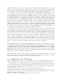
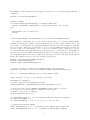
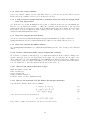
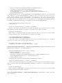
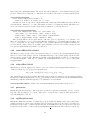
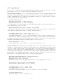
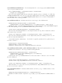
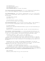
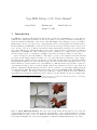
Figure 1: Large FEM deformations: The crane cubic (voxel) mesh is shown blended on top of the embedded triangle mesh, whereas the dragon uses the external surface of the tetrahedral mesh for rendering.
Original triangle models are courtesy of Waldemar Barkowski, http://www.artworx-media.de, and Stanford Computer Graphics Laboratory, http://graphics.stanford.edu/data/3Dscanrep/, respectively.
1
(executable) simulator to interactively test the implemented materials, timestepping methods, and other
settings. Several example meshes and configuration files are included to demonstrate the various materials.
We provide a lot of usage advice and detailed experiments on the performance of Vega in [SSB12]. Please
refer to this paper for the theoretical background and explanation of the implemented methods.
Vega provides co-rotational linear Finite Element Method (FEM) elasticity [MG04] (and the exact
tangent stiffness matrix [Bar12], similar to [CPSS10]), orthotropic linear materials (combined with corotational FEM) [LB14], Saint-Venant Kirchhoff FEM deformable models (see [Bar07]), invertible FEM
models [ITF04, TSIF05], and mass-spring systems. All models can simulate quality large deformations and
include support for multi-core computing. Vega provides linear materials, as well as neo-Hookean, SaintVenant Kirchhoff and Mooney-Rivlin nonlinear materials (combined with invertible FEM [ITF04, TSIF05]).
Optional compression resistance term [KTY09] is available to improve simulation stability for soft materials.
Arbitrary nonlinear materials can be added to Vega. For isotropic hyperelastic materials, this is as easy as
defining an energy function and its first and second derivatives. Implemented integrators include implicit
backward Euler [BW98], explicit central differences [Wri02], implicit Newmark [Wri02] and symplectic Euler. Other integrators can be added easily. Vega also includes an implementation of the Baraff-Witkin cloth
solver [BW98], model reduction [BJ05], and rigid body dynamics [BW01].
Finally, we find it useful to also state what Vega currently does not support. Vega currently supports
3D solid simulation on volumetric meshes, as well as cloth simulations on triangle meshes; it does not
support strands. It uses linearized tets and axis-aligned cubes for mesh elements; higher-order elements are
not supported. Vega solves linear systems of equations using preconditioned conjugated gradients or direct
sparse solvers. It does not incorporate solver acceleration strategies such as multigrid. It does not implement
inverse kinematics, or space-time optimization. Vega does not simulate articulated rigid bodies or fluids.
It does not support mesh cutting or other run-time mesh modifications; although mesh material properties
could be altered at run-time without much difficulty. While it does not incorporate collision detection or
contact resolution, it is possible to use any external collision detection library, compute forces externally,
and set them as external forces in Vega. A more elaborate contact solver could be written by using Vega’s
routines to compute internal forces and stiffness matrices in arbitrary mesh configurations.
New in Vega 2.0: improved isotropic materials (greatly improved behavior for soft materials via compression resistance [KTY09]), model reduction (implementation of Jernej Barbič model reduction work [BJ05],
reducedStVK, integratorDense classes), cloth solver (implementation of Baraff-Witkin’s cloth model [BW98];
clothBW class), rigid body simulation (implementation Baraff-Witkin SIGGRAPH 2001 course notes [BW01],
rigidBodyDynamics class), quaternion arithmetics (quaternion class), load/save images in PNG, JPEG,
TIFF, TGA, PPM formats (wrappers to libpng, libjpeg and libtiff; TGA and PPM are built-in), imageIO
class), several bug fixes and documentation improvements.
New in Vega 2.1: orthotropic materials (materials that exhibit different stiffnesses in three orthogonal
directions, see [LB14]), documentation improvements, binary .vegb format, faster loading of volumetric
meshes with many regions, support for the clang compiler (Mac), bug fixes.
1.1
Compiling Vega: Core Functionality
This section explains how to build the “core” functionality of Vega, i.e., (unreduced) simulations of 3D solid
elasticity. This functionality has been available in Vega since version 1.0 (with some improvements).
Vega is designed to be cross-platform. We have successfully compiled it on Linux, Windows and Mac OS
X. We provide makefiles (make command) for Linux and Mac OS X. The easiest approach to build Vega is
to go to the Vega root folder, and launch ./build. If all goes well, this should compile the entire Vega core
functionality. Details are below.
The first step is to select either Makefile-headers/Makefile-header.linux, or
Makefile-headers/Makefile-header.osx, depending on your OS. By default, linux is selected. The selection is made by creating a soft link Makefile-headers/Makefile-header that points to the selected
Makefile. To switch to MAC OS X, use:
cd Makefile-header;ln -sf Makefile-header.osx Makefile-header.
2
Alternatively, you can switch using the provided scripts Makefile-headers/selectLinux or
Makefile-headers/selectMACOSX.
To compile the entire set of libraries and the interactive simulator in one step, move to the
utilities/interactiveDeformableSimulator folder and run $ make. To compile an individual library
libraryName, along with all the libraries it depends on, move to libraries/libraryName and run $ make.
The script ./build combines Makefile-header selection and the compilation into one step.
To clean all the compiled files (for the interactive simulator and for all the libraries), move to
utilities/interactiveDeformableSimulator and run $ make deepclean. To only clean the simulator
folder, run $ make clean. Similarly, running $ make deepclean in folder libraries/libraryName will
clean the folder for libraryName as well as those of all the other libraries libraries it depends on, whereas
running $ make clean will only clean the libraries/libraryName folder.
Dependencies: Vega has no required external dependencies. It includes all the necessary components for
deformable object simulation. If you want to use the optional model reduction functionality (introduced in
version 2.0), you will need the dependencies listed in Section 1.3.1. Vega uses its own CG solver as the default
solver for implicit integration. This solver can be substituted for external linear system sparse solvers such
as PARDISO or SPOOLES. Other solvers can be easily added as well. The provided demonstration driver
uses OpenGL for visualization: it depends on the GL, GLU, GLUT OpenGL libraries. It also depends on the
GLUI User Interface Library, which is used for the driver’s user interface (buttons, edit boxes, etc.). This
external library (LGPL license) is included with the Vega distribution (in libraries/glui), unmodified as it
was downloaded from http://glui.sourceforge.net/. The provided Makefiles will automatically compile
GLUI to a shared library (to comply with the LGPL license terms), and link it to the driver. On some systems,
for the build to work correctly, you may need to figure out how to satisfy the dependencies on OpenGL and/or
GLUI. Default settings for the locations of all libraries are provided in the Makefile-header files for Linux and
Mac OS X. If needed, custom locations can be set by modifying the libraries/include/openGL-headers.h
header. For example, to set custom locations and names of the OpenGL libraries, modify the LIBRARIES,
STANDARD LIBS, GLUI DIR, GLUI INCLUDE, and GLUI LIB variables in Makefile-header.
Using PARDISO: Vega contains code to easily use the PARDISO solver from the Intel MKL library. To
use PARDISO, you must first install it. To specify the names and locations of PARDISO libraries, modify the
PARDISO DIR, PARDISO INCLUDE, and PARDISO LIB variables in the Makefile-header. If needed, adjust the
included MKL header files by modifying the libraries/include/lapack-headers.h header file. Next, notify Vega that PARDISO is available by defining (uncommenting) the macro PARDISO SOLVER IS AVAILABLE
in libraries/sparseSolver/sparseSolverAvailability.h. Finally, switch the integrator library to
PARDISO by enabling (defining) the macro PARDISO in libraries/integrator/integratorSolverSelection.h.
Then, recompile Vega and the driver.
Using SPOOLES: Vega can also use SPOOLES, a public domain sparse solver, freely available at http:
//www.netlib.org/linalg/spooles/. The library is used by the SPOOLESSolver and SPOOLESSolverMT
classes in the sparseSolver library. To use SPOOLES, follow the same steps as with PARDISO. To set
the location of the SPOOLES library and header files, modify the SPOOLES DIR, SPOOLES INCLUDE, and
SPOOLES LIB variables in Makefile-header.
Note that the PARDISO and SPOOLES solvers are not necessary to compile our example driver. By default,
Vega uses its preconditioned conjugate solver (PCG), available in libraries/sparseSolver/CGSolver.h.
Note, however, that Intel MKL gives the fastest computation; about 30% faster than SPOOLES and much
faster than PCG. PARDISO or SPOOLES are also more stable than PCG, because they can handle system
matrices that have negative eigenvalues (indefinite systems). Finally, note that the make files do not monitor the openGL-headers.h or lapack-headers.h files, so modifications to these may require cleaning and
remaking the project, as explained above.
Using OpenMP: In a couple of places, Vega uses OpenMP to accelerate the computation. OpenMP is
not used for any core Vega functionality and so performance of Vega is mostly unaffected by whether you use
3
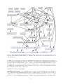
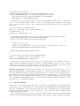
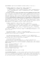
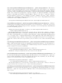
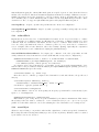
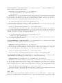
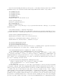
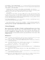
Figure 2: The dependencies of libraries in Vega. Blue colors denotes non-core libraries that are not
necessary for the main Vega functionality or to build the demonstration driver. Dashed libraries are model
reduction libraries.
OpenMP or not. For example, internal force and stiffness matrix calculators use pthreads and are unaffected
by the discussion in this paragraph. Most important usage of OpenMP is in the LargeModalDeformationFactory
where the different modal derivatives can be computed in parallel using OpenMP. In addition to that,
OpenMP is used to accelerate the parallel loading of multiple binary obj and volumetric meshes (new in
Vega FEM 2.1). By default, OpenMP support is disabled. If you want to enable it, uncomment the following
line in Makefile-header and recompile Vega.
OPENMPFLAG=-fopenmp -DUSE_OPENMP
Microsoft Visual Studio: The pthreads library is required for the multi-threading functionality in
Vega. This library ships with Linux and Mac OS X operating systems. For Windows, you can download
a Windows port of pthreads from http://sources.redhat.com/pthreads-win32/. In order to build
the driver, one needs a GLUT implementation, for example, http://user.xmission.com/~nate/glut.html.
4
The stdlib.h which ships with the recent versions of Visual Studio may have a conflict with some GLUT
implementations. To fix this issue, right click on the project name in the Solution Explorer tab and select
Properties→C/C++→Preprocessor→Preprocessor definitions. Then append GLUT BUILDING LIB to the
existing definitions, separated by semicolons.
1.2
Driver Executable and Examples
Vega provides a complete simulation driver (executable), as well as several complete examples. Examples include all the necessary meshes and configuration files. To run the simulator on these configurations, run any of
the run [modelname] shell scripts in the examples folder. For example, try examples/turtle/run turtle,
examples/asianDragon/run asianDragon or examples/asianDragon/run asianDragon unconstrained.
You can read the examples/guideToExamples.txt for a brief overview of our examples. The simulator
executable interactiveDeformableSimulator takes one command-line argument: a .config configuration
file such as those in the examples folder. The .config file specifies such information as the mesh, the
desired material and timestepping method to use, the timestep, damping, an optional secondary rendering
mesh embedded in the deformable mesh, and so on. The simulator must be run in the folder containing
the desired .config file, since this file contains relative paths to other files read by the executable. It is
easiest to achieve this by using the provided run* shell scripts. Inside the simulator, some useful keys are
’E’, ’e’, and ’w’, to toggle the displays of embedded rendering mesh, volumetric mesh, and volumetric mesh
wireframe, respectively. Note that the main simulation window must have focus for the keys to work.
1.3
Compiling Vega: Model Reduction
In order to build model reduction, you must first build the “core” functionality (previous section).
Important: For model reduction, Pardiso solver must be available. Therefore, you must install it, and
uncomment the #DEFINE PARDISO SOLVER IS AVAILABLE line in
libraries/sparseSolver/sparseSolverAvailability.h. This step must be done **before** building
the core Vega functionality. In case you already previously compiled “core” functionality, go to
utilities/interactiveDeformableSimulator and run make deepclean, then fix
sparseSolverAvailability.h and recompile “core” functionality using ./build.
Before you can build model reduction, you must also satisfy all the dependencies (below). Once you have
done so, you can issue the ./buildModelReduction script in the main Vega folder. If all goes well, this should
compile all the model reduction libraries, as well as the demonstration driver reducedDynamicSolver-rt
and the preprocessor application LargeModalDeformationFactory.
1.3.1
Model Reduction Dependencies
The model reduction part of Vega has the following dependencies: Intel MKL (Pardiso), GLEW, Cg (Nvidia),
ARPACK and wxWidgets. You must install all the required dependencies and
edit the Makefile-headers/Makefile-header file accordingly.
• Intel MKL: provides a dense and sparse linear solver. Both a dense and sparse solver are required
for model reduction. On some platforms, such as Mac OS X, the dense solver is built-in into the
operating system (the framework “Accelerate”), and therefore Intel MKL is not needed for the dense
solves. For the sparse linear solver, we typically use the Pardiso solver from Intel MKL, but SPOOLES
is a good free alternative. By using SPOOLES or PCG, and an external dense solver, it is possible
to completely eliminate the need for Intel MKL. To control what solver is used, set the macros in
libraries/sparseSolver/sparseSolverAvailability.h.
• GLEW: needed to access OpenGL extensions. This is a standard, free, library.
• Cg: needed for GP-GPU shaders to compute vertex deformations (u = U q) on the GPU
(ObjMeshGPUDeformer library). This is a free library that can be downloaded from the Nvidia website.
• ARPACK: needed to solve large sparse eigenproblems in the LargeModalDeformationFactory. Available free of charge (BSD license) at http://www.caam.rice.edu/software/ARPACK/. In order to
5
compile ARPACK, you will need a fortran compiler. We use gfortran, the standard Fortran compiler
that ships with gcc on Unix systems.
• wxWidgets: this is the UI library used in the LargeModalDeformationFactory. Available free of
charge at http://www.wxwidgets.org.
1.3.2
Model Reduction Drivers
LargeModalDeformationFactory: Given a simulation mesh (tetrahedral or voxel), its material properties (may be non-homogeneous), and a set of constrained vertices, this application driver generates a
fast reduced deformable model suitable for fast large-deformation simulation, as described in [BJ05]. The
driver supports the St. Venant-Kirchhoff material, i.e., linear isotropic material parameterized by Young’s
moduli and Poisson’s ratios. The application starts either with a triangle mesh or a volumetric mesh,
and generates all the necessary data for a subsequent real-time simulation. You can then run a real-time
simulation from your own code using ImplicitNewmarkDense and StVKReducedInternalForces classes.
The application supports tetrahedral and voxel 3D volumetric meshes. The application also contains several generally useful sub-components: compute linear modes (via ARPACK) of arbitrary volumetric (tet or
voxel) meshes, under arbitrary boundary conditions (including free boundary conditions), compute modal
derivatives, compute volumetric mesh mass and stiffness matrix, create cube volumetric meshes for arbitrary
input triangle geometry. The application outputs several files, which are loadable by various Vega classes.
For example, it produces the cubic polynomial of reduced internal forces that you can then load using the
StVKReducedInternalForces and ImplicitNewmarkDense classes and timestep in your own code. All the
modal matrices generated (linear modes, modal derivatives, or simulation basis matrix) can be loaded using
the ”Matrix” class. If you want to use tetrahedral meshes, you can generate them using the TetGen mesh
generation package. It is possible to compute the modal derivatives in parallel, using OpenMP. This will
give a significant boost to the model reduction pre-processing pipeline. To do so, enable the USE OPENMP
macro in the header of modalDerivatives.cpp, and then add -fopenmp to the CXXFLAGS macro in your
Makefile-headers/Makefile-header file.
reducedDynamicSolver-rt: This is an example driver that demonstrates how to launch a run-time model
reduction simulation (created via LargeModalDeformationFactory). In utilities/reducedDynamicSolver-rt,
there are two example demos: run A, run simpleBridge.
1.4
Short Tutorial on Using Vega
Vega is a middleware library and should be integrated with the rest of the user’s C/C++ code. In this
section, we give the typical steps to do so. Details on the specific methods can be found in subsequent
sections. The first step is to load a volumetric mesh from a .veg file (format is described in Section 1.5),
which creates a VolumetricMesh object. It is easiest to do so using the provided VolumetricMeshLoader
class, which automatically detects the type of elements in the mesh (tets or cubes).
#include "volumetricMeshLoader.h"
...
char inputFilename[96] = "myInputMeshFile.veg";
VolumetricMesh * volumetricMesh = VolumetricMeshLoader::load(inputFilename);
if (volumetricMesh == NULL)
printf("Error: failed to load mesh.\n");
else
printf("Success. Number of vertices: %d . Number of elements: %d .\n",
volumetricMesh->getNumVertices(), volumetricMesh->getNumElements());
At this point, the mesh and its material properties have been parsed into memory, and we have a valid
VolumetricMesh object. Next, we will initialize a specific 3D deformable model, allowing us to compute
internal forces and stiffness matrices for arbitrary deformed object configurations. Let us use the corotational
6
linear FEM model. Because that model only supports tet meshes, we need to first check if the mesh is indeed
a TetMesh.
#include "corotationalLinearFEM.h"
...
TetMesh * tetMesh;
if (volumetricMesh->getElementType() == VolumetricMesh::TET)
tetMesh = (TetMesh*) volumetricMesh; // such down-casting is safe in Vega
else
{
printf("Error: not a tet mesh.\n");
exit(1);
}
CorotationalLinearFEM * deformableModel = new CorotationalLinearFEM(tetMesh);
Note that the down-casting can be avoided if the mesh is known to be a tet mesh: simply initialize
TetMesh directly using the constructor in the TetMesh class. We now have a valid deformable model, and
it is possible to query internal forces and tangent stiffness matrices in any mesh configuration. Typically,
however, we want to timestep the model in time. So let’s proceed with building an integrator for the model.
We need to first create a ForceModel object, to connect our deformable model to an integrator. We also
need the mass matrix, and specify which model vertices (if any) are to be fixed. Then, we can initialize the
integrator. Let us use the implicit backward Euler integrator. Note that the sparse linear system solver to
use for implicit integration is selected by editing the file ”integratorSolverSelection.h” inside the Integrator
library. The default selection is to use Vega’s conjugate gradient solver.
#include "corotationalLinearFEMForceModel.h"
#include "generateMassMatrix.h"
#include "implicitBackwardEulerSparse.h"
...
// create the class to connect the deformable model to the integrator
ForceModel * forceModel = new CorotationalLinearFEMForceModel(deformableModel);
int r = 3 * tetMesh->getNumVertices(); // total number of DOFs
double timestep = 0.0333; // the timestep, in seconds
SparseMatrix * massMatrix;
// create consistent (non-lumped) mass matrix
GenerateMassMatrix::computeMassMatrix(tetMesh, &massMatrix, true);
// This option only affects PARDISO and SPOOLES solvers, where it is best
// to keep it at 0, which implies a symmetric, non-PD solve.
// With CG, this option is ignored.
int positiveDefiniteSolver = 0;
// constraining vertices 4, 10, 14 (constrained DOFs are specified 0-indexed):
int numConstrainedDOFs = 9;
int constrainedDOFs[9] = { 12, 13, 14, 30, 31, 32, 42, 43, 44 };
// (tangential) Rayleigh damping
double dampingMassCoef = 0.0; // "underwater"-like damping (here turned off)
double dampingStiffnessCoef = 0.01; // (primarily) high-frequency damping
7
// initialize the integrator
ImplicitBackwardEulerSparse * implicitBackwardEulerSparse = new
ImplicitBackwardEulerSparse(r, timestep, massMatrix, forceModel,
positiveDefiniteSolver, numConstrainedDOFs, constrainedDOFs,
dampingMassCoef, dampingStiffnessCoef);
At this point, we can start timesteping our model! By default, initial conditions are zero deformation
and zero velocity. Arbitrary initial conditions could be set via IntegratorBase::SetState. Let us apply
some forces to the model, perform a couple of timesteps, and read the results. The forces are specified in
Newtons (N).
// alocate buffer for external forces
double * f = (double*) malloc (sizeof(double) * r);
int numTimesteps = 10;
for(int i=0; i<numTimesteps; i++)
{
// important: must always clear forces, as they remain in effect unless changed
implicitBackwardEulerSparse->SetExternalForcesToZero();
if (i == 0) // set some force at the first timestep
{
for(int j=0; j<r; j++)
f[j] = 0; // clear to 0
f[37] = -500; // apply force of -500 N to vertex 12, in y-direction, 3*12+1 = 37
implicitBackwardEulerSparse->SetExternalForces(f);
}
implicitBackwardEulerSparse->DoTimestep();
}
// alocate buffer to read the resulting displacements
double * u = (double*) malloc (sizeof(double) * r);
implicitBackwardEulerSparse->GetqState(u);
And that’s it – these were all the necessary steps to use Vega! The array u now contains the mesh vertex
displacements after 10 simulation timesteps. We can now continue simulating, render the object, or perform
collision detection (using some external software). We could then set the resulting contact forces as the
external forces so that they will affect the deformations in the subsequent steps.
Choosing the timestep: The unit for the timestep is seconds (s). It is very important to choose a
sufficiently small timestep so that the simulation is stable. Too large timesteps will lead to simulation blowup. If the simulation is unstable, the first step should always be to greatly decrease the timestep and see
if the simulation is stable. Some integrators are inherently more stable than others, e.g., implicit backward
Euler is more stable than implicit Newmark (but introduces more artificial damping). Also, direct sparse
solvers (PARDISO and SPOOLES) tend to be more stable than Conjugate Gradients. For many more such
usage tips, refer to our publication [SSB12].
1.5
Vega file formats
In this section, we document the Vega file format, .veg. This is a text (ASCII) file format which is flexible
and the files are easy to edit manually; we recommend that new users familiarize themselves with this format
first. Since Vega FEM 2.1, Vega also supports a binary file format, .vegb, which can be used when smaller
file sizes and faster loading times are desired. The usage of .vegb is documented in the VolumetricMesh,
TetMesh and CubicMesh classes.
The .veg format extends the open source volumetric mesh file format developed by Jonathan Shewchuk
and employed by Stellar [KS09, Kli08] and TetGen [Han11] mesh generation packages. Meshes in Shewchuk’s
8
format are easily loadable into Vega. Note that the Stellar webpage [KS09] contains a converter script that
can convert other popular mesh formats into the Stellar/TetGen format.
For simulation, it is necessary to specify mesh material properties, in addition to geometry. The Vega file
format .veg achieves this by introducing a set of additional keywords for material specification. Vega
supports heterogeneous material properties, i.e., different parts of the mesh can have different material
properties. In the extreme case, every mesh element can have a separate set of material properties. We
provide several example .veg meshes in the models folder. For heterogeneous material properties, see the
turtle example in models/turtle.
Basics: The Vega file format is ASCII. Lines starting with * denote a command. Lines starting with #
are comments. Empty lines are ignored. Files can be nested using the *INCLUDE command. The effect of
*INCLUDE is to include, at that point in the .veg file, the entire contents of the included file. Include files
can include other files; they can nest arbitrarily.
Vertices are specified using the *VERTICES keyword. The second line gives the number of vertices, followed
by integer “3” (three-dimensional simulation), optionally followed by more parameters, which are ignored.
The subsequent lines give one vertex per line, in the format:
<vertex index> <x> <y> <z>
where the vertex index starts either at 0 or 1, increments by 1 for every vertex. The unit for vertex positions
is meters [m]. Example:
*VERTICES
5 3 0 0
1 0.5 0.5 0.5
2 1.0 -0.5 0.5
3 -1.0 0.0 1.0
4 0.25 -0.25 0.5
5 0.6 0.2 0.3
Elements are specified using the *ELEMENTS keyword. The second line gives the element type, either
“TET” or “CUBIC”. Tetrahedra can have arbitrary shape. Of course, degenerate tetrahedra should be
avoided, whereas tetrahedra with small dihedral angles generally cause a higher linear system condition
number, which may cause instabilities. Use of a quality tet mesh generator is advisable. Cubic meshes must
consist of cubes: all sides of cubes must be equal; general cuboids (boxes) are not supported. Cubes must
be axis-aligned. The third line gives the number of mesh elements, followed by the number of vertices in
each element (4 for tets and 8 for cubes), followed by some optional integers that are ignored. Subsequent
lines give one element per line, in the format:
<element index> <vertex 1> ... <vertex n>
where the element index starts either at 0 or 1 and increments by 1 for every element, and n is the number
of element vertices. For tet, n = 4, for cubes, n = 8. Example:
*ELEMENTS
TETS
2 4 0
1 2 3 4 1
2 5 3 4 1
specifies a mesh with two tets. The first tet has vertices 2, 3, 4, 1 (in that order), and the second tet has
vertices 5, 3, 4, 1. The ordering of vertices within the element matters. Incorrect order will give wrong results.
For tet meshes, tets must be oriented so that vertices 1, 2, 3, 4 specify the tet in a positive orientation, i.e.,
((v2 − v1 ) × (v3 − v1 )) · (v4 − v1 ) ≥ 0. If the input mesh does not have this property (or you are unsure), you
can call the function orient in the TetMesh class to establish a correct orientation. Note that the meshes
9
produced by TetMesh have positive orientation. For cubic meshes, the vertices must be specified in the
following order: (0, 0, 0), (1, 0, 0), (1, 1, 0), (0, 1, 0), (0, 0, 1), (1, 0, 1), (1, 1, 1), (0, 1, 1). This example specifies
the unit cube; cubes whose lower-left-front corner is not at the origin and/or whose size is not unit must be
specified analogously. Other orders will give wrong results.
New in Vega 2.0: vertices and elements can now be numbered starting either at 0, or at 1. They must
be given in a sorted, ascending order, starting either from 0 or 1. Previous versions of Vega only supported
starting at 1. Support for 0 was added to accommodate the recent versions of TetGen, which produce tet
meshes with vertices and elements starting at 0. The following tet mesh is valid in Vega 2.0, and equivalent
to the tet mesh given above:
*VERTICES
5 3 0 0
0 0.5 0.5 0.5
1 1.0 -0.5 0.5
2 -1.0 0.0 1.0
3 0.25 -0.25 0.5
4 0.6 0.2 0.3
*ELEMENTS
TETS
2 4 0
0 1 2 3 0
1 4 2 3 0
Materials are specified using the *MATERIAL keyword. The first line gives the material name, the second
line specifies the material properties. Three material specifications are supported: “ENU”, for any material
that is parameterized by Young’s modulus (E, in N/m2 ) and Poisson’s ratio (ν, dimensionless quantity (no
unit)), “MOONEYRIVLIN” for Mooney-Rivlin materials, and “ORTHOTROPIC” for orthotropic materials.
All materials include a mass density specification, in kg/m3 .
Most materials in Vega use the “ENU” specification: co-rotational linear FEM, StVK, invertible StVK,
invertible neo-Hookean, etc. Example:
*MATERIAL mat1
ENU, 1000, 1E8, 0.40
specifies a material with mass density 1000 kg/m3 , Young’s modulus of 108 N/m2 , and Poisson’s ratio of 0.4.
The Mooney-Rivlin material can be simulated using the invertible FEM class IsotropicHyperelasticFEM
and is specified as follows:
*MATERIAL myMaterialName
MOONEYRIVLIN, 500, 0.5, 0.6, 1.0
specifies a Mooney-Rivlin material with mass density 500 kg/m3 , µ01 = 0.5, µ10 = 0.6 and v1 = 1.0. The
implemented Mooney-Rivlin material is described in Section 3.5.5 of [Bow09].
Orthotropic materials [LB14] are materials that exhibit different stiffnesses in three orthogonal directions.
By default, the orthogonal directions are (1, 0, 0), (0, 1, 0), (0, 0, 1), but arbitrary orthogonal directions are
supported. The implemented orthotropic material supports large deformations and is described in [LB14].
Orthotropic materials in Vega can be simulated using the corotational linear FEM deformable model available
in the CorotationalLinearFEM class. Vega supports several formats to specify an orthotropic material, based
on whether the user wants to specify an orthotropic material in full generality, or how many values the user
wants to leave at the default settings.
10
*MATERIAL myMaterialName
ORTHOTROPIC, 500, 1E8, 2E8, 3E8, 0.4, 0.45, 0.5, 5E7, 8E7, 7E7, 0.866025, -0.5,
0, 0.5, 0.866025, 0, 0, 0, 1
(the entire specification starting from ORTHOTROPIC must be on one line)
This is the default format for orthotropic materials. It specifies the parameters for an orthotropic material
with mass density 500 kg/m3 , Young’s moduli (“stiffnesses”) E1 = 108 N/m2 , E2 = 2 × 108 N/m2 , E3 =
3 × 108 N/m2 in the three orthogonal directions, Poisson’s ratios (“volume preservation coefficient”) ν12 =
0.4, ν23 = 0.45, ν31 = 0.5, shear moduli µ12 = 5 × 107 N/m2 , µ23 = 8 × 107 N/m2 , µ31 = 7 × 107 N/m2 and
a 3 × 3 rotation matrix Q in row-major order representing the orientation of the three orthotropic principal
axes. Note that there are six Poisson’s ratios νij , for i 6= j, only three of which are independent. Formulas for
ν21 , ν32 , ν13 are in [LB14]. Briefly, Ei gives the stiffness of the material when loaded in orthogonal direction
i. Poisson’s ratio νij gives the contraction in direction j when the material extends (stretches) in direction
i. See [LB14] for details on the meaning of the parameters. Young’s moduli must satisfy the conditions
Ei > 0, for i = 1, 2, 3. This format gives the user full control over orthotropic materials. However, the user
must ensure that the elasticity tensor of this material is positive-definite, otherwise the simulation might be
unstable. The conditions involve all Ei and νij , and are available in [LB14]. The rotation Q is


0.866025
−0.5
0
0.5
0.866025 0  ,
(1)
Q=
0
0
1
i.e., a rotation by 30 degrees around the z-axis. First orthogonal axis is (0.866025, 0.5, 0) (stiffness E1 =
108 N/m2 ), second axis is (−0.5, 0.866025, 0) (stiffness E2 = 2 × 108 N/m2 ), and the third axis is (0, 0, 1)
(stiffness E3 = 3 × 108 N/m2 ) in this example.
*MATERIAL myMaterialName
ORTHOTROPIC_N3G3R9, 500, 1E8, 2E8, 3E8, 0.4, 0.45, 0.5, 5E7, 8E7, 7E7, 0.866025, -0.5,
0, 0.5, 0.866025, 0, 0, 0, 1
(the entire specification starting from ORTHOTROPIC_N3G3R9 must be on one line)
specifies the same material as above with all independent parameters. In other words, ORTHOTROPIC and
ORTHOTROPIC N3G3R9 are identical.
*MATERIAL myMaterialName
ORTHOTROPIC_N3G3, 500, 1E8, 2E8, 3E8, 0.4, 0.45, 0.5, 5E7, 8E7
specifies an orthotropic material with mass density 500 kg/m3 , Young’s moduli E1 = 108 N/m2 , E2 = 2 ×
108 N/m2 , E3 = 3 × 108 N/m2 , Poisson’s ratios ν12 = 0.4, ν23 = 0.45, ν31 = 0.5, shear moduli µ12 =
5 × 107 N/m2 , µ23 = 8 × 107 N/m2 , µ31 = 7 × 107 N/m2 and a default orientation where the three principal
axes are aligned with the world coordinate axes, i.e., Q is identity.
*MATERIAL myMaterialName
ORTHOTROPIC_N1G1R9, 500, 1E8, 2E8, 3E8, 0.4, 1.1, 0.866025, -0.5,
0, 0.5, 0.866025, 0, 0, 0, 1
(the entire specification starting from ORTHOTROPIC_N1G1R9 must be on one line)
specifies an orthotropic material in a simplified, but stable way, using a single Poisson’s ratio-like parameter
ν, as described in [LB14]. Mass density is 500 kg/m3 , Young’s moduli are E1 = 108 N/m2 , E2 = 2 ×
108 N/m2 , E3 = 3 × 108 N/m2 , Poisson’s ratio-like parameter is ν = 0.4, and the shear moduli scaling
factor is µ = 1.1. This format also specifies a 3 × 3 rotation matrix Q in row-major order representing the
orientation of the three orthotropic principal axes. This format uses the method described in [LB14] to
produce a material that is guaranteed to be stable. Parameter ν must satisfy −1 < ν < 1/2. It is used to
create a set of stable Poisson’s ratios. The user can tune ν like the Poisson’s ratio in an isotropic material.
This format also uses an automatic method to compute shear moduli from E1 , E2 , E3 and ν; the formulas
are given in [LB14]. Parameter µ scales the shear moduli computed by the method of [LB14]. A value of
µ = 1 means that the shear moduli computed by [LB14] will be used unmodified. Values µ > 1 will increase
shear stresses (make the model shear less), whereas values 0 < µ < 1 will decrease shear stresses (make the
model shear more).
11
*MATERIAL myMaterialName
ORTHOTROPIC_N1G1, 500, 1E8, 2E8, 3E8, 0.4, 1.1
specifies an orthotropic material in the same way as ORTHOTROPIC N1G1R9, except that the rotation is
assumed to be identity, i.e., a default orientation where the three principal axes are aligned with the world
coordinate axes. Mass density is 500 kg/m3 , Young’s moduli are E1 = 108 N/m2 , E2 = 2 × 108 N/m2 , E3 =
3 × 108 N/m2 , Poisson’s ratio-like parameter is ν = 0.4, and the shear moduli scaling factor is µ = 1.1.
*MATERIAL myMaterialName
ORTHOTROPIC_N1R9, 500, 1E8, 2E8, 3E8, 0.4, 0.866025, -0.5,
0, 0.5, 0.866025, 0, 0, 0, 1
specifies an orthotropic material in the same way as ORTHOTROPIC N1G1R9, except that µ is assigned the
default value µ = 1. Mass density is 500 kg/m3 , Young’s moduli are E1 = 108 N/m2 , E2 = 2×108 N/m2 , E3 =
3 × 108 N/m2 , Poisson’s ratio-like parameter is ν = 0.4.
*MATERIAL myMaterialName
ORTHOTROPIC_N1, 500, 1E8, 2E8, 3E8, 0.4
specifies an orthotropic material in the same way as ORTHOTROPIC N1G1, except that µ is assigned the
default value µ = 1. Mass density is 500 kg/m3 , Young’s moduli are E1 = 108 N/m2 , E2 = 2×108 N/m2 , E3 =
3 × 108 N/m2 , Poisson’s ratio-like parameter is ν = 0.4.
Sets store a set of integer indices. They are used to store indices of elements that share the same material
(=region). First line specifies the set name, followed by a comma-separated list of set elements. Elements
should be sorted and identified by the indices given in the *ELEMENTS section, i.e., either 0-indexed or
1-indexed, depending on whether *ELEMENTS are given 0-indexed or 1-indexed. Example:
*SET set1
11, 17, 21, 37, 113, 220, 310, 555,
556, 557, 570, 601, 991, 1013, 1210, 1225
Regions: Elements that share material properties are organized into regions. A region is specified using a
*REGION keyword. For example,
*REGION
set1, material1
creates a region consisting of the elements specified in the Set set1, and assigns material material1 to it.
In order to set the entire mesh to a material, you can use the built-in set allElements:
*REGION
allElements, material1
If the union of all specified regions does not contain all mesh elements, the remaining elements are assigned
a material as follows. The assigned material is the last material mentioned in the .veg if the file specified
at least one material. If no material was specified, the default material is assigned to the entire mesh. The
default material is of type “ENU”, with default parameters E = 106 N/m2 , ν = 0.45, ρ = 1000kg/m3 , where
E is Young’s modulus, ν is Poisson’s ratio and ρ is mass density. If specification of regions was omitted from
a .veg file, the entire mesh is assigned the default material.
Easy re-use of Stellar/TetGen meshes: Suppose that the mesh vertices and elements are stored in
myMesh.node and myMesh.ele files, in the standard Stellar/TetGen format. The following “template” .veg
file is the shortest way to import those meshes into Vega:
12
*VERTICES
*INCLUDE myMesh.node
*ELEMENTS
TETS
*INCLUDE myMesh.ele
Of course, material properties and regions could be appended as described in the previous paragraphs.
1.6
Acknowledging
If you use Vega, we will appreciate if you acknowledge it. Please use the following citation:
Jernej Barbič, Fun Shing Sin, Daniel Schroeder:
Vega FEM Library. 2012. http://www.jernejbarbic.com/vega
Here is the BibTeX file:
@misc{Vega,
author =
"Jernej Barbi\v{c} and Fun Shing Sin and Daniel Schroeder",
title =
"{Vega FEM Library}",
year = "2012",
note = "http://www.jernejbarbic.com/vega",
}
1.7
1.7.1
FAQ
How can I create volumetric meshes for use with Vega?
Vega does not provide meshing capabilities. However, any 3D tet or cubic mesh can be loaded into Vega
(.veg file format). You can use any external mesher, such as for example TetGen, or Stellar. There are
many commercial meshers available.
1.7.2
What is the .veg file format?
Before Vega, there was no free file format to specify 3D volumetric meshes with material properties. So, we
extended the popular free format of Jonathan Shewchuk, which can specify 3D geometry, to also support
mesh material properties. Meshes given in Shewchuk’s format (such as those produced by TetGen, or Stellar)
are trivially loadable into Vega. If material specification is omitted, default material parameters are assigned
to the entire mesh. See the above sections for the documentation of the .veg file format. The .veg file
format is free.
1.7.3
What is the .vegb file format?
This is a binary file format, offering the same functionality as .veg. It was introduced in Vega FEM 2.1, so
that files can be made smaller and loading times decreased. So, since Vega FEM 2.1., users have a choice
between .veg and .vegb.
1.7.4
Can Vega simulate non-homogeneous material properties?
Yes. See the turtle example where the backshell was made 100x stiffer than the rest of the turtle.
1.7.5
Can Vega simulate free-flying (unconstrained) deformable objects?
Yes. Simply specify zero constraints when initializing the integrator.
13
1.7.6
How can I resolve collisions?
Vega does not include collision detection capabilities. However, you can use any external collision detection
library, and set the resulting contact forces as external forces in Vega.
1.7.7
I want to embed a triangle mesh into a volumetric mesh, and render the triangle mesh.
Does Vega support this?
Yes. It should be noted that all simulations in Vega run on volumetric meshes (except cloth simulations).
However, you can transfer (in real-time, or offline) the volumetric mesh deformations to the embedded
triangle mesh using the interpolate routine in the VolumetricMesh class. The technique uses barycentric
interpolation. You can see this in the turtle example (and other examples). See the source code of the
interactiveDeformableSimulator driver.
1.7.8
How can I compute the mass matrix?
You can use utilities/volumetricMeshUtilities/generateMassMatrix. It calls a routine from
generateMassMatrix.h in the volumetricMesh library, which you can call directly from your code.
1.7.9
How can I compute the stiffness matrix?
Use GetTangentStiffnessMatrix (or ComputeStiffnessMatrix) in any of the several provided material
classes.
1.7.10
Is there a MS Visual Studio project (solution) file available?
We don’t have one right now, although Vega does compile under Windows. In the workspace, simply create
separate entries (projects) for each Vega library, then compile each one separately. Do the same for the
driver. Make sure you don’t mix Multithreaded and Multithreaded DLL, as it may lead to linking errors.
You may want to add post-compile events which copy the newly created .lib (as well as header files .h) into
some canonical folder, so that other libraries and the driver can reference it.
1.7.11
What are the physical units used in Vega?
Input 3D meshes: meters (m)
Time: seconds (s)
Forces: Newton (N)
Young’s modulus: Pa=N/m^2
Poisson’s ratio: no unit (dimensionless)
1.7.12
How are the invariants I, II, III defined (for isotropic materials)?
Vega follows the definition in the reference [BW08]:
I = tr(C) = λ21 + λ22 + λ23 ,
2
II = tr(C ) =
λ41
III = det(C)
+ λ42 + λ43 ,
= λ21 λ22 λ23 .
(2)
(3)
(4)
Some other references, however, define II as
II 0 = λ21 λ22 + λ22 λ23 + λ23 λ21 .
It is possible to easily convert from II to II 0 ; the two are related via I 2 .
14
(5)
1.7.13
Where can I learn more about FEM, deformable objects, and the methods implemented in Vega?
Our research paper on Vega (published in the Computer Graphics Forum Journal [SSB12]) explains the
implemented methods and analyzes the performance of Vega. You can also read the cited papers, and
visit the webpage of the SIGGRAPH 2012 course on FEM for deformable object simulation: http://www.
femdefo.org.
1.7.14
I like Vega. I have used it in a commercial application, and want to donate funding.
You are under no obligation to do so. If you want to donate funding, this is of course welcome; the funds
will be used for further academic research on Vega and deformable object simulation. In any case, we will
appreciate if you let us know that you used Vega in your application.
2
Libraries
Below is a listing of the libraries in the libraries folder. The purpose of each library as a whole is
described, and more specific information is given on selected constituent classes and member functions
to highlight important functionality. For subclasses, virtual functions are only re-listed if the subclass
implements a previously-abstract function or substantially alters its functionality. Note that a few functions
allocate memory which must be deleted by the caller: you can recognize such functions by the ** (pointer
to pointer) calling convention. As standard in C/C++, the memory is allocated with malloc/free for the
built-in datatypes, and new/delete for all the other datatypes.
2.1
camera
class SphericalCamera Provides utilities for setting the OpenGL camera based upon a spherical-coordinate
system centered at a specified focus point.
void Look()
Applies the current camera transformation to the active OpenGL matrix. Note that this does not run
glMatrixMode or glLoadIdentity.
void MoveRight(double amount)
void MoveUp(double amount)
void MoveIn(double amount)
void ZoomIn(double amount)
Move the camera by a user-specified offset. Supply negative values to move/zoom in the opposite direction.
void SavePosition(const char * filename)
void LoadPosition(const char * filename)
Save or load the camera position to a file. LoadPosition prints a warning if the specified file does not
exist.
2.2
clothBW
Implements the well-known Baraff-Witkin cloth simulator [BW98]. Input is a triangle mesh with material
properties such as stretch, shear and bend resistance. The library can compute both the internal elastic
forces and their gradient (tangent stiffness matrix). It computes stretch, shear, and bend forces. For bend
forces, the user can choose to use the input angle as the rest bend angle, or use the zero angle. Baraff-Witkin
damping is not implemented, but you can use the damping provided by the Vega integrator class. In order
to timestep the cloth, use the integratorSparse library. In this way, you can create cloth animations under
any specified external forces. For collisions, you need to use some external library to compute the contact
forces on the cloth, and then set them as external forces to the simulator.
15
class ClothBW
Implements the Baraff-Witkin cloth simulator [BW98], as described above.
ClothBW(int numParticles, double * masses, double * restPositions,
int numTriangles, int * triangles, int * triangleGroups,
int numMaterialGroups, double * groupTensileStiffness, double * groupShearStiffness,
double * groupBendStiffnessU, double * groupBendStiffnessV, double * groupDamping,
int addGravity=0)
Creates the cloth elastic model, from a given triangle mesh. Variable numParticles specifies the number of particles (vertices of the triangle mesh), masses is an array of length numParticles that gives the
masses of each particle, restPositions is an array of length 3× numParticles and gives the rest positions of the particles, three values (x, y, z) per each particle, triangles is an integer array of length 3×
numTriangles giving integer indices of the three particles forming a triangle, triangleGroups is an integer array of length numTriangles giving the integer index of the material group to which each triangle
belongs, groupTensileStiffness, groupShearStiffness, groupBendStiffnessU, groupBendStiffnessV
and groupDamping are arrays that give the scalar stiffness and damping parameters for each material group.
All indices in the class are 0-indexed. This constructor does not require triangleUVs input; it computes
suitable UVs automatically. The UVs are continuous only within each triangle; the UV map is not global.
This is sufficient for isotropic simulation; but cannot accommodate anisotropic effects.
ClothBW(int numParticles, double * masses, double * restPositions,
int numTriangles, int * triangles, double * triangleUVs, int * triangleGroups,
int numMaterialGroups, double * groupTensileStiffness, double * groupShearStiffness,
double * groupBendStiffnessU, double * groupBendStiffnessV, double * groupDamping,
int addGravity=0)
A variant of the constructor where the UVs are not computed automatically, but are provided by the
caller. Parameter triangleUVs is a double array of length 3 × 2× numTriangles, indicating the uv coordinates for every vertex.
void ComputeForce(double * u, double * f, bool addForce=false)
Computes the total cloth force on every vertex. Parameter u (length 3×numParticles) gives the displacements of all vertices away from the rest configuration.
void ComputeStiffnessMatrix(double * u, SparseMatrix * K, bool addMatrix=false)
Computes the tangent stiffness matrix (gradient of cloth forces). Parameter u (length 3×numParticles)
gives the displacements of all vertices away from the rest configuration.
void SetComputationMode(bool mode[4])
Specifies what cloth forces and stiffness matrices are to be computed by ComputeForce and
ComputeStiffnessMatrix, AddForce and AddStiffnessMatrix. This allows users to toggle on/off computation of the stretch/shear forces, bend forces, stretch/shear bend stiffness matrices, and bend stiffness
matrix, as follows:
mode[0]:
mode[1]:
mode[2]:
mode[3]:
computeStretchAndShearForce: yes/no
computeBendForce: yes/no
computeStretchAndShearStiffnessMatrices: yes/no
computeBendStiffnessMatrices: yes/no
Default value is true for all fields of mode.
class ClothBWMT
Multi-threaded version of ClothBW.
class ClothBWFromObjMesh A convenience class that constructs a cloth model from an obj mesh. The
mesh need not be triangulated; if it is non-triangular, faces will be split into triangles automatically. There
are two member functions GenerateClothBW. One sets constant material properties for all the triangles, and
the other allows the specification of specific material properties for each obj mesh material (.mtl file).
16
2.3
configFile
class ConfigFile Parses values from a text configuration file. The syntax of the configuration file is userdefined. Options can be read as int, bool, float, double, and char * (C-string) types. See any of the
.config files in the examples folder for an example of the config file syntax.
int addOption(const char * optionName, T * destLocation)
Defined for T as int, bool, float, double, char. Adds a mandatory option with name optionName.
When the config file is later parsed, any value found for this option is written to the variable pointed to by
destLocation. If no value for this option is found, the parse is considered to have failed. Returns a non-zero
value if the option has already been defined.
int addOptionOptional(const char * optionName, T * destLocation, T defaultvalue)
int addOptionOptional(const char * optionName, char * destLocation, const char * defaultvalue)
Adds an optional option with name optionName. When the config file is later parsed, the variable pointed
to by destLocation is set to the value found in the file, or to defaultValue if no value is set. Returns a
non-zero value if the option has already been defined.
int parseOptions(const char * filename)
Parses the options in file filename, writing the option values it reads to the appropriate variables. A
non-zero value is returned if any mandatory options are not specified.
2.4
corotationalLinearFEM
class CorotationalLinearFEM Implements the corotational linear finite element model described in [MG04].
The class can also compute the exact tangent stiffness matrix; the implementation is described in [Bar12].
CorotationalLinearFEM(TetMesh * tetMesh)
Initializes the model based upon an input tetrahedral mesh.
void GetStiffnessMatrixTopology(SparseMatrix ** stiffnessMatrixTopology)
Writes to *stiffnessMatrixTopology a newly allocated (using new) zero matrix containing the pattern
of non-zero entries of the stiffness matrix.
void ComputeForceAndStiffnessMatrix(double * vertexDisplacements,
double * internalForces, SparseMatrix * stiffnessMatrix, int warp=1)
Computes the internal forces and stiffness matrix given a vector vertexDisplacements of the displacements for the vertices of the tetrahedral mesh. If either internalForces or stiffnessMatrix is NULL, the
function does not calculate or return the corresponding information. The warp parameter controls whether
the simulation “warps” stiffnesses and therefore supports large deformations. When warping is enabled
(warp=1 or warp=2), the implementation supports large deformations. The default is warp=1, in which
case the simulation uses the approximate tangent stiffness matrix as described in [MG04]. For warp=2,
the class computes the exact tangent stiffness matrix; our implementation is described in [Bar12]. Such
an exact matrix has better simulation properties; however, it requires approximately 1.5x the computation
time of the approximate matrix. If warping is disabled (warp=0), one obtains the standard linear FEM
simulation [Sha90]. Such simulation runs faster than the warped simulations because it timesteps the linear
equation M ü + Du̇ + Ku = f. It is only accurate under small displacements.
2.5
elasticForceModel
Provides implementation of the ForceModel base class for the deformable models supported by Vega. This
makes it possible to use these deformable models with the integrators in Vega (integrator library).
17
class CorotationalLinearFEMForceModel : public ForceModel Exposes the internal force- and
stiffness matrix-calculating functionality of the CorotationalLinearFEM material using the common interface
of ForceModel.
CorotationalLinearFEMForceModel(CorotationalLinearFEM *
corotationalLinearFEM, int warp=1)
Sets the CorotationalLinearFEM object for force and stiffness calculations. The parameter warp has
the same meaning as in the CorotationalLinearFEM class.
void SetWarp(int warp)
Sets the warp parameter. This makes it possible to change the warp parameter at runtime.
class MassSpringSystemForceModel : public ForceModel Exposes the internal force- and stiffness
matrix-calculating functionality of the mass-spring material using the common interface of ForceModel.
MassSpringSystemForceModel(MassSpringSystem * massSpringSystem)
Sets the MassSpringSystem object used for force and stiffness calculations.
class StVKForceModel : public ForceModel Exposes the internal force- and stiffness matrix-calculating
functionality of the StVK material using the common interface of ForceModel.
StVKForceModel(StVKInternalForces * stVKInternalForces,
StVKStiffnessMatrix * stVKStiffnessMatrix = NULL)
Sets the StVK objects used for internal forces and stiffness calculations. If no StVKStiffnessMatrix is
provided, one is constructed based upon stVKInternalForces.
class IsotropicHyperelasticFEMForceModel : public ForceModel Exposes the internal force- and
stiffness matrix-calculating functionality of the invertible FEM materials using the common interface of
ForceModel.
IsotropicHyperelasticFEMForceModel(
IsotropicHyperelasticFEM * isotropicHyperelasticFEM)
Sets the invertible-elements object used for internal forces and stiffness matrix calculations.
2.6
forceModel
This library provides the abstract base class for a force model used in the integratorSparse library, i.e., a
“black-box” function u 7→ fint (u) and its gradient in
M ü + αM + βK(u) + D u̇ + fint (u) = fext .
Any dynamical system described by such a differential equation can then be timestepped by the integrator
library, by providing an implementation of fint and its gradient, in a class derived from ForceModel.
For deformable simulations, class ForceModel connects integrators to internal forces and tangent stiffness
matrix calculator classes. This allows the different deformable models in Vega to expose their internal forces
and stiffness matrices to the integrator in a uniform way. Derived classes that implement fint and its gradient
for the deformable models in Vega can be found in the library elasticForceModel. The reason for why
library forceModel is separated from elasticForceModel is so that the integratorSparse library can be
compiled and used independently from any deformable materials in Vega. Similarly, one can compile and use
forceModel and elasticForceModel independently of integratorSparse, making it possible to timestep
the Vega deformable models with externally provided integrators.
18
class ForceModel Abstract base class for a force model fint (u) whose gradient (typically the tangent
stiffness matrix) is a sparse matrix. All deformable models in Vega fall into this category. Note: dense
gradient matrices occur in applications involving model reduction.
int Getr()
Returns r, the number of object degrees of freedom (typically three times the number of vertices or
particles). Note that the r member variable must be set by a subclass.
virtual void GetInternalForce(double * u, double * internalForces) = 0
The internal forces arising from vertex displacements u are written to the array internalForces. Must
be implemented by derived classes.
virtual void GetTangentStiffnessMatrixTopology(SparseMatrix **
tangentStiffnessMatrix) = 0
Allocates (new) a SparseMatrix with the correct pattern of non-zero entries to hold a stiffness matrix for
this material, and write the matrix pointer to *tangentStiffnessMatrix. Must be implemented by derived
classes.
virtual void GetTangentStiffnessMatrix(double * u,
SparseMatrix * tangentStiffnessMatrix) = 0
The tangent stiffness matrix arising from vertex displacements u is written to the previously allocated
tangentStiffnessMatrix. Must be implemented by derived classes.
virtual void GetForceAndMatrix(double * u, double *
internalForces, SparseMatrix * tangentStiffnessMatrix)
Writes out the internal forces and stiffness matrix arising from displacements u, using the implementations
of the functions above. May be overloaded by derived classes.
2.7
getopts
int getopts(int argc, char **argv, opt t opttable[])
Parses the argc and argv from a main function and extracts any specified option values. Modified from
public domain code by Paul Edwards.
2.8
glslPhong
Implements per-pixel (Phong) lighting using a GLSL shader.
2.9
graph
class Graph Stores an undirected graph. The vertices of the graph are represented by the integers from 0
to the number of vertices minus one, and the graph structure is constant after being set in the constructor.
Graph(int numVertices, int numEdges, int * edges)
Initializes the graph, giving it numVertices vertices and numEdges edges. The input array of integers
edges encodes the edges as subsequent pairs of vertex indices.
int IsNeighbor(int vtx1, int vtx2)
Returns 0 if vertices vtx1 and vtx2 are not neighbors, and returns 1 plus the index of vtx2 in the list of
vtx1’s neighbors otherwise.
19
2.10
hashTable
Implements a simple 1D hash table. Keys are of type ’unsigned int’, and datatype can be arbitrary (templated).
2.11
imageIO
Loads and saves PNG, TIFF and JPEG, TGA, PPM file formats. In order to use PNG, JPEG or TIFF,
you must enable them in the file ”imageFormats.h”, and recompile the code, and then link against libpng,
libjpeg and libtiff libraries, respectively. PPM and TGA are built-in. They need not be enabled (they are
always enabled) and require no linking against external libraries.
class ImageIO
2.12
Performs the functionality described above.
insertRows
Provides utilities for the insertion and removal of elements from dense 1D arrays. This is useful, for example,
when constraining (fixing) vertices in a deformable simulation.
void InsertRows(int mFull, double * xConstrained, double * x,
int numFixedRows, int * fixedRows, int oneIndexed=0)
Copies xConstrained into x, and then inserts zeros into x. Zeroes are placed among the elements at each
index indicated in fixedRows, until the total desired size mFull of the output array is reached. x is assumed
to be already allocated.
void RemoveRows(int mFull, double * xConstrained, double * x,
int numFixedRows, int * fixedRows, int oneIndexed=0)
Copies x into xConstrained, and then removes the elements at the indices given in fixedRows from
xConstrained. xConstrained is assumed to be already allocated.
void FullDOFsToConstrainedDOFs(int mFull, int numDOFs,
int * DOFsConstrained, int * DOFs, int numFixedRows,
int * fixedRows, int oneIndexed=0)
Translates indices of elements in an unreduced array to the indices which would contain those same
elements in the reduced array produced by calling RemoveRows with fixedRows. Input is DOFs and output
is DOFsConstrained. Writes to DOFsConstrained[i] the index in the reduced array that would give the
element at index DOFs[i] in the unreduced array.
2.13
integrator
This is the “base” library for numerical integration in Vega. Together with “derived” libraries integratorSparse
and integratorDense, it provides several implicit and explicit integrators to solve equations of the form
M ü + αM + βK(u) + D u̇ + fint (u) = fext .
(6)
For a broader discussion of this equation, please see [SSB12]. The integrator library itself only consists
of abstract base classes. You must use either integratorSparse or integratorDense for the actual integration. The sparse library (integratorSparse) is designed for systems (6) where M, D, K are (large)
sparse matrices, e.g., geometrically complex deformable objects (without model reduction). The dense library (integratorDense), in turn, is designed for systems (6) where M, D, K are dense matrices, e.g., for
model reduction simulations.
20
class IntegratorBase Serves as a base class to all the integrators. The class stores displacements, velocities, and accelerations for the simulation internally, and provides access to modify these buffers, but offers no
actual timestepping capabilities; this is deferred to derived classes. The class also holds Rayleigh damping
coefficients that specify how much the mass and stiffness matrix contribute to the damping matrix.
IntegratorBase(int r, double timestep,
double dampingMassCoef=0.0, double dampingStiffnessCoef=0.0)
Sets the number of degrees of freedom r, timestep timestep, and coefficients for how much to add the
mass matrix and stiffness matrix to the damping matrix. Allocates (malloc) a number of internal buffers of
r doubles for holding the current displacement, velocity, internal forces, and so on.
virtual ~IntegratorBase()
Frees (free) the internal buffers.
virtual void ResetToRest()
Sets the internal position, velocity, and acceleration buffers to zero.
virtual int SetState(double * q, double * qvel=NULL) = 0
Resets internal position buffer to the values in q, and does likewise for internal velocity buffer if qvel is
not NULL. Returns 0 if successful, 1 otherwise.
void SetqState(const double * q, const double * qvel=NULL, const double * qaccel=NULL)
void GetqState(double * q, double * qvel=NULL, double * qaccel=NULL)
Copies external position, velocity, and/or acceleration buffers to the internal buffers, or vice versa. Each
buffer is copied only if the pointer to the external buffer is not NULL.
void SetExternalForces(double * externalForces)
void AddExternalForces(double * externalForces)
void GetExternalForces(double * externalForces)
Sets or adds the values from externalForces to the external forces buffer, or writes the external forces
buffer to externalForces.
virtual void SetTimestep(double timestep)
double GetTimestep()
Sets or returns the timestep value.
virtual int DoTimestep() = 0
Performs a timestep of the simulation, given the current values in the internal/external forces, position,
velocity, and acceleration buffers. The resulting position, velocity, and acceleration are saved to these buffers.
Returns 0 if and only if the timestep is completed without error.
2.14
integratorSparse
This library can timestep systems (6) where M, D, K are (large) sparse matrices, e.g., geometrically complex
deformable objects (without model reduction). This is the “core” integrator capability in Vega. For model
reduction, see integratorDense.
class IntegratorBaseSparse : public IntegratorBase A base class for integrators for dynamical systems characterized by (large) sparse matrices, such as geometrically complex 3D elasticity. This is the main
integrator type in Vega. These integrators use a ForceModel class to obtain the internal forces and stiffness
matrices. Stiffness matrices are sparse and stored using the SparseMatrix class. IntegratorBaseSparse
stores two sparse matrices: the mass matrix and the damping matrix to be applied in addition to mass- and
stiffness-based damping specified in IntegratorBase.
21
IntegratorBaseSparse(int r, double timestep, SparseMatrix * massMatrix,
ForceModel * forceModel, int numConstrainedDOFs=0, int * constrainedDOFs=NULL,
double dampingMassCoef=0.0, double dampingStiffnessCoef=0.0)
Initializes the number of degrees of freedom r, the timestep, the mass matrix, which degrees of freedom
are constrained, and the ForceModel. The internal damping SparseMatrix is set to zero.
virtual void SetForceModel(ForceModel * forceModel)
Sets the ForceModel object to forceModel. This makes it possible to change the force model at runtime.
virtual void SetDampingMatrix(SparseMatrix * dampingMatrix)
Sets the damping matrix D to dampingMatrix. This matrix will be added to the matrix produced
according to the mass and stiffness damping coefficients to get the total damping matrix for the simulation.
virtual double GetForceAssemblyTime()
virtual double GetSystemSolveTime()
Return the time taken in DoTimestep to generate the force/stiffness values and to solve the linear system
while timestepping, respectively. It is up to subclasses to calculate these values in DoTimestep.
virtual double GetKineticEnergy()
virtual double GetTotalMass()
Calculates and returns the kinetic energy or total mass of the simulation, based upon the mass matrix
and the velocity buffer of the class.
class ImplicitNewmarkSparse : public IntegratorBaseSparse Implements implicit Newmark integration, and expands IntegratorBaseSparse with features common to Newmark-style integrators.
ImplicitNewmarkSparse(int r, double timestep,
SparseMatrix * massMatrix, ForceModel * forceModel,
int positiveDefiniteSolver=0, int numConstrainedDOFs=0,
int * constrainedDOFs=NULL, double dampingMassCoef=0.0,
double dampingStiffnessCoef=0.0, int maxIterations = 1,
double epsilon = 1E-6, double NewmarkBeta=0.25,
double NewmarkGamma=0.5, int numSolverThreads=0)
Initializes maxIterations, epsilon, NewmarkBeta, NewmarkGamma, and
numSolverThreads parameters, and forwards the other parameters to the
IntegratorBaseSparse constructor. For PARDISO and SPOOLES solvers, we found best performance with
2-3 threads; more threads usually decreased performance.
virtual void SetTimestep(double timestep)
Sets the timestep.
virtual int SetState(double * q, double * qvel=NULL)
Sets the position (and optionally the velocity) buffer, and calculates the acceleration buffer accordingly
using implicit Newmark, assuming no external force. Returns 0 if successful, 1 otherwise.
virtual int DoTimestep()
Runs a timestep of implicit Newmark, updating the internal position, velocity, and acceleration buffers
accordingly. Returns 0 if and only if the timestep is completed successfully.
void SetNewmarkBeta(double NewmarkBeta)
void SetNewmarkGamma(double NewmarkGamma)
Set the value of the beta and gamma parameters, respectively, for Newmark integrators. No checking is
performed to see if these values are in the appropriate range.
22
void UseStaticSolver(bool useStaticSolver)
Sets whether to use a static solver. The class defaults to dynamic.
class ImplicitBackwardEulerSparse : public ImplicitNewmarkSparse
ward Euler integration [BW98].
Implements implicit back-
ImplicitBackwardEulerSparse(int r, double timestep,
SparseMatrix * massMatrix,
ForceModel * forceModel,
int positiveDefiniteSolver=0, int numConstrainedDOFs=0,
int * constrainedDOFs=NULL, double dampingMassCoef=0.0,
double dampingStiffnessCoef=0.0, int maxIterations = 1,
double epsilon = 1E-6, int numSolverThreads=0)
Initializes the integrator.
virtual int SetState(double * q, double * qvel=NULL)
Sets the position (and optionally the velocity) buffer based on the parameters, and calculates the appropriate acceleration buffer values using implicit Euler, assuming no external forces. Returns 0 if successful, 1
otherwise.
virtual int DoTimestep()
Runs a timestep of implicit Euler, and updates the internal position, velocity, and acceleration buffers
accordingly. Returns 0 if successful, 1 otherwise.
class CentralDifferencesSparse : public IntegratorBaseSparse Implements the explicit central differences integrator.
CentralDifferencesSparse(int numDOFs, double timestep,
SparseMatrix * massMatrix,
ForceModel * forceModel,
int numConstrainedDOFs=0, int * constrainedDOFs=NULL,
double dampingMassCoef=0.0, double dampingStiffnessCoef=0.0,
int tangentialDampingMode=1, int numSolverThreads=0)
Initializes the integrator settings via the IntegratorBaseSparse constructor, and selects the number of
threads to use for the sparse linear solver. Tangential damping mode controls how often the Rayleigh damping
matrix is recomputed. This damping matrix depends on the tangent stiffness matrix, which changes in time.
When 0, the damping matrix is never updated. The system matrix is then constant, so one can factor it
only once. However, this is not recommended for large deformations as it leads to damping artifacts. When
tangentialDampingMode > 0, the damping matrix is updated every “tangentialDampingMode”th timestep.
Default is 1, i.e., update at every timestep.
virtual int SetState(double * q, double * qvel=NULL)
Sets the position (and optionally velocity) buffers. Always returns 0.
virtual int DoTimestep()
Runs a timestep of explicit central differences, and updates the internal position, velocity and acceleration
buffers accordingly. Returns 0 if successful, 1 otherwise.
class EulerSparse : public IntegratorBaseSparse Implements explicit Euler integration, with a flag
to enable symplectic Euler integration. Because this class never forms the tangent stiffness matrix, damping
is controlled via mass-based damping only.
EulerSparse(int r, double timestep, SparseMatrix * massMatrix,
23
ForceModel * forceModel,
int symplectic=0, int numConstrainedDOFs=0,
int * constrainedDOFs=NULL, double dampingMassCoef=0.0)
Initializes the integrator settings via the IntegratorBaseSparse constructor, and sets whether to perform
symplectic integration.
virtual int SetState(double * q, double * qvel=NULL)
Sets the position (and optionally velocity) buffers based on the parameters, and sets the acceleration
buffer via explicit (or symplectic) Euler assuming no external forces. Returns 0 if successful, 1 otherwise.
virtual int DoTimestep()
Runs a timestep of explicit (or symplectic) Euler, and updates the internal position, velocity, and acceleration buffers accordingly. Returns 0 if successful, 1 otherwise.
2.15
integratorDense
This library can timestep systems (6) where M, D, K are dense matrices. While this functionality is generalpurpose, its main purpose in Vega is model reduction. This class largely parallels integratorSparse, with
the class names simply renamed from “Sparse” to “Dense”. For standard (non-model reduction) simulation
in Vega, see integratorSparse.
class IntegratorBaseDense : public IntegratorBase A base class for integrators for dynamical systems characterized by dense matrices. These integrators use a ReducedForceModel class to obtain the
internal forces and stiffness matrices. Stiffness matrices are dense and stored in column-major format.
IntegratorBaseDense(int r, double timestep, double * massMatrix,
ReducedForceModel * reducedForceModel,
double dampingMassCoef=0.0, double dampingStiffnessCoef=0.0)
Initializes the number of degrees of reduced freedom r, the timestep, the mass matrix, and the ReducedForceModel.
The internal damping is set to zero.
void SetReducedForceModel(ReducedForceModel * reducedForceModel)
Sets the ReducedForceModel object to reducedForceModel. This makes it possible to change the force
model at runtime.
virtual void SetMassMatrix(double * massMatrix)
Sets the reduced mass matrix to massMatrix. This makes it possible to change the mass matrix at
runtime.
virtual double GetForceAssemblyTime()
virtual double GetSystemSolveTime()
Return the time taken in DoTimestep to generate the force/stiffness values and to solve the linear system
while timestepping, respectively. It is up to subclasses to calculate these values in DoTimestep.
virtual double GetKineticEnergy()
virtual double GetTotalMass()
Calculates and returns the kinetic energy or total mass of the simulation, based upon the mass matrix
and the velocity buffer of the class.
class ImplicitNewmarkDense : public IntegratorBaseDense Implements implicit Newmark integration, and expands IntegratorBaseDense with features common to Newmark-style integrators. This is
the integrator used in [BJ05].
ImplicitNewmarkDense(int r, double timestep,
24
double * massMatrix, ReducedForceModel * reducedForceModel,
solverType solver=positiveDefiniteMatrixSolver,
double dampingMassCoef=0.0, double dampingStiffnessCoef=0.0,
int maxIterations = 1, double epsilon = 1E-6, double NewmarkBeta=0.25,
double NewmarkGamma=0.5)
Initializes maxIterations, epsilon, NewmarkBeta, and NewmarkGamma parameters, and forwards the
other parameters to the IntegratorBaseDense constructor. There are three choices for the dense solver:
positive-definite, symmetric, general. Positive-definite solver is the most common choice (and cca 2x faster
than other options). However, if the system matrix becomes singular (rare; only extreme deformations), an
error will be issued. To specify the solver, use one of the three choices: solverType::generalMatrixSolver,
solverType::symmetricMatrixSolver, solverType::positiveDefiniteMatrixSolver.
virtual void SetTimestep(double timestep)
Sets the timestep.
virtual int SetState(double * q, double * qvel=NULL)
Sets the position (and optionally the velocity) buffer, and calculates the acceleration buffer accordingly
using implicit Newmark, assuming no external force. Returns 0 if successful, 1 otherwise.
virtual int DoTimestep()
Runs a timestep of implicit Newmark, updating the internal position, velocity, and acceleration buffers
accordingly. Returns 0 if and only if the timestep is completed successfully.
void SetNewmarkBeta(double NewmarkBeta)
void SetNewmarkGamma(double NewmarkGamma)
Set the value of the beta and gamma parameters, respectively, for Newmark integrators. No checking is
performed to see if these values are in the appropriate range.
void UseStaticSolver(bool useStaticSolver)
Sets whether to use a static solver. The class defaults to dynamic.
class ImplicitBackwardEulerDense : public IntegratorBaseDense Implements implicit backward
Euler integration [BW98], for dense stiffness matrices.
ImplicitBackwardEulerDense(int r, double timestep,
double * massMatrix,
ReducedForceModel * reducedForceModel,
solverType solver=positiveDefiniteMatrixSolver, double dampingMassCoef=0.0,
double dampingStiffnessCoef=0.0, int maxIterations = 1,
double epsilon = 1E-6)
Sets the integrator parameters with the ImplicitNewmarkDense constructor.
virtual int SetState(double * q, double * qvel=NULL)
Sets the position (and optionally the velocity) buffer based on the parameters, and calculates the appropriate acceleration buffer values using implicit Euler, assuming no external forces. Returns 0 if successful, 1
otherwise.
virtual int DoTimestep()
Runs a timestep of implicit Euler, and updates the internal position, velocity, and acceleration buffers
accordingly. Returns 0 if successful, 1 otherwise.
class CentralDifferencesDense : public IntegratorBaseDense
ferences integrator.
25
Implements the explicit central dif-
CentralDifferencesDense(int numDOFs, double timestep,
double * massMatrix,
ReducedForceModel * reducedForceModel,
double dampingMassCoef=0.0, double dampingStiffnessCoef=0.0,
int tangentialDampingMode=1)
Initializes the integrator settings via the IntegratorBaseDense constructor. Tangential damping mode
controls how often the Rayleigh damping matrix is recomputed. This damping matrix depends on the tangent
stiffness matrix, which changes in time. When 0, the damping matrix is never updated. The system matrix
is then constant, so one can factor it only once. However, this is not recommended for large deformations
as it leads to damping artifacts. When tangentialDampingMode > 0, the damping matrix is updated every
“tangentialDampingMode”th timestep. Default is 1, i.e., update at every timestep.
virtual int SetState(double * q, double * qvel=NULL)
Sets the position (and optionally velocity) buffers. Always returns 0.
virtual int DoTimestep()
Runs a timestep of explicit central differences, and updates the internal position, velocity and acceleration
buffers accordingly. Returns 0 if successful, 1 otherwise.
2.16
isotropicHyperelasticFEM
Provides classes to calculate the energy, internal forces and stiffness matrices of a variety of invertible material
methods.
class IsotropicHyperelasticFEM Provides an implementation of the invertible FEM method presented
in [ITF04]. Also computes the tangent stiffness matrix as presented in [TSIF05]. Supports isotropic hyperelastic materials with energy defined in terms of the three invariants I, II, III. A few such example materials
are provided, and the user can define her own custom materials simply by deriving from IsotropicMaterial.
IsotropicHyperelasticFEM(TetMesh * tetMesh, IsotropicMaterial * isotropicMaterial,
double inversionThreshold=-DBL MAX, bool addGravity=false, double g=9.81)
Initializes the invertible FEM method. Before creating this class, you must first create the tet mesh, and
create an instance of the IsotropicMaterial material (e.g., NeoHookeanIsotropicMaterial). Parameter
inversionThreshold controls when the inversion prevention mechanism activates. If the principal stretches
are smaller than the inversionThreshold, they will be clamped to that, which will generally prevent element
inversion. For example, a typical inversionThreshold value would be 0.1. By default, inversion handling is
disabled (inversionThreshold=−∞). Values of 1.0 or higher should not be used. The isotropicMaterial
must be pre-created: you can use one of our provided classes, or derive from the IsotropicMaterial to
create your own custom isotropic hyperelastic materials.
The material properties are determined as follows. If the isotropicMaterial is of the “Homogeneous”
kind (for example, HomogeneousNeoHookeanIsotropicMaterial), then the material properties are homogeneous and are specified by isotropicMaterial; material properties in the tetMesh are ignored (only
geometry is used). If, however, the isotropicMaterial is not of the “Homogeneous” kind (for example,
NeoHookeanIsotropicMaterial), then the material properties are such as specified in the tetMesh and
isotropicMaterial class (and may be non-homogeneous).
Internally, the constructor reads the mesh tetMesh, pre-computes the area weighted vertex normals, the
inverse of the Dm (as in [ITF04]), and the derivative of the deformation gradient with respect to the vertex
displacements.
double ComputeEnergy(double * vertexDisplacements)
Given the array vertexDisplacements of vertex displacements from rest position, returns the non-linear
elastic strain energy of the mesh. The energy is calculated based upon the principal stretches of the SVDdiagonalized deformation gradients of the individual mesh elements.
26
void ComputeForces(double * vertexDisplacements, double * internalForces)
Given the array vertexDisplacements of vertex displacements, writes the resulting vertex forces to
the pre-allocated array internalForces. Forces are calculated from the principal stretches of the SVDdiagonalized deformation gradients of the individual mesh elements.
void GetStiffnessMatrixTopology(SparseMatrix ** stiffnessMatrixTopology)
Allocates (new) a SparseMatrix with the correct pattern of non-zero entries to hold a stiffness matrix
for this material, and writes the matrix pointer to *tangentStiffnessMatrix.
void GetTangentStiffnessMatrix(double * u, SparseMatrix * tangentStiffnessMatrix)
Writes the stiffness matrix arising from vertex displacements u to the pre-allocated tangentStiffnessMatrix.
The stiffness matrix is calculated based upon the principal stretches and rotation matrices from the SVD
diagonalization of the deformation gradient of each element.
class IsotropicMaterial Serves as an abstract base class for isotropic hyperelastic materials which define
energy in terms of the three invariants I, II, III. This classes is then derived into classes that implement
concrete isotropic materials. The class represents the material of a single element (tet or cube). The definition
of the invariants used in Vega FEM is as follows:
I = tr(C) = λ21 + λ22 + λ23 ,
2
II = tr(C ) =
λ41
III = det(C)
+ λ42 + λ43 ,
= λ21 λ22 λ23 ,
(7)
(8)
(9)
where λi are the principal stretches (singular values of the deformation gradient F ), and C = F T F is the
right Cauchy-Green deformation tensor. Note that in the literature, there are at least two ways to define II.
The above invariants are defined in [BW08]. Some other references define the second invariant as
II 0 = λ21 λ22 + λ22 λ23 + λ23 λ21 .
(10)
Such an invariant can be easily converted to the invariants used by Vega, and back, II 0 = (I 2 − II)/2.
virtual double ComputeEnergy(int elementIndex, double * invariants) = 0
Returns the energy of the element given the three invariants invariants[0], invariants[1], and
invariants[2]. The integer variable elementIndex makes it possible to make the material properties vary
from element to element (heterogeneous material properties).
virtual void ComputeEnergyGradient(int elementIndex,
double * invariants, double * gradient) = 0
Given the three invariants invariants[0],invariants[1],invariants[2] computes the derivative of
the energy with respect to the invariants and writes the result to gradient[0],gradient[1],gradient[2].
virtual void ComputeEnergyHessian(int elementIndex,
double * invariants, double * hessian) = 0
Given the three invariants invariants[0],invariants[1],invariants[2] computes the second derivative of the energy with respect to the invariants and writes the result to hessian where hessian[0] =
∂ 2 Ψ/∂I 2 , hessian[1] = ∂ 2 Ψ/∂I∂II, hessian[2] = ∂ 2 Ψ/∂I∂III, hessian[3] = ∂ 2 Ψ/∂II 2 , hessian[4]
= ∂ 2 Ψ/∂II∂III, and hessian[5] = ∂ 2 Ψ/∂III 2
To define your own isotropic hyperelastic material, simply derive from IsotropicMaterial and implement functions ComputeEnergy, ComputeEnergyGradient, ComputeEnergyHessian.
27
class IsotropicMaterialWithCompressionResistance : public IsotropicMaterial This abstract
class is the same as IsotropicMaterial, except it adds the ability for the derived classes to use compression
resistance. Compression resistance is an extra energy term which prevents the material from undergoing large
compression. Such a capability makes the material more volume preserving and improves simulation stability.
All the derived classes in Vega implement compression resistance as explained in [KTY09]. Compression
resistance is internally scaled with the material stiffness. Therefore, the value of compression resistance
has (approximately) equal effect on the simulation regardless of stiffness. In practice, using compression
resistance improves simulation quality and stability. It also produces better looking simulations under large
deformations. Its use is highly recommended.
IsotropicMaterialWithCompressionResistance(int enableCompressionResistance=0)
class StVKIsotropicMaterial : public IsotropicMaterialWithCompressionResistance StVK material that supports spatially varying material parameters. Provides functions to compute the energy, gradient, and Hessian of the StVK material given the three invariants I, II, III. The implemented StVK material
is described in [BW08], page 158.
StVKIsotropicMaterial(TetMesh * tetMesh, int enableCompressionResistance=0,
double compressionResistance=0.0)
The material parameters are read from the tet mesh, and are cached in the constructor. Parameter
compressionResistance must be non-negative. The larger the value, the more the material resists compression. Value of 0 means that there is no resistance; this is equivalent to setting enableCompressionResistance
to 0. A reasonable value of compressionResistance is 500.0. High values will require smaller timesteps,
or else the simulation may go unstable. Largest values we typically tried in practice were in 10,000s, e.g.,
50,000. The constructor throws an exception if the provided tet mesh does not consist of materials specifying
E, ν.
class HomogeneousStVKIsotropicMaterial : public IsotropicMaterialWithCompressionResistance StVK material with homogeneous (spatially global) material parameters. Provides functions to
compute the energy, gradient, and Hessian of the StVK material given the three invariants I, II, III. Compression resistance is as described in [KTY09].
HomogeneousStVKIsotropicMaterial(double E, double nu,
int enableCompressionResistance=0, double compressionResistance=0.0)
Initializes the Young’s modulus E and the Poisson ratio nu of the material.
class NeoHookeanIsotropicMaterial : public IsotropicMaterialWithCompressionResistance NeoHookean material that supports spatially varying material parameters. Provides functions to compute the
energy, gradient, and Hessian of the Neo-Hookean material given the three invariants I, II, III. The implemented neo-Hookean material is described in [BW08], page 162.
NeoHookeanIsotropicMaterial(TetMesh * tetMesh,
int enableCompressionResistance=0, double compressionResistance=0.0)
The material parameters are read from the tet mesh, and are cached in the constructor. Throws an
exception if the provided tet mesh does not consist of materials specifying E, ν.
class HomogeneousNeoHookeanIsotropicMaterial : public IsotropicMaterialWithCompressionResistance Neo-Hookean material with homogeneous (spatially global) material parameters. Provides
functions to compute the energy, gradient, and Hessian of the neo-Hookean material given the three invariants I, II, III.
HomogeneousNeoHookeanIsotropicMaterial(double E, double nu,
int enableCompressionResistance=0, double compressionResistance=0.0)
28
Initializes the Young’s modulus E and the Poisson ratio nu of the material.
class MooneyRivlinIsotropicMaterial : public IsotropicMaterialWithCompressionResistance
Mooney-Rivlin material that supports spatially varying material parameters.
MooneyRivlinIsotropicMaterial(TetMesh * tetMesh,
int enableCompressionResistance=0, double compressionResistance=0.0)
The material parameters are read from the tet mesh, and are cached in the constructor. Throws an
exception if the provided tet mesh does not consist of Mooney-Rivlin materials. Provides functions to
compute the energy, gradient, and Hessian of the Mooney-Rivlin material given the three invariants I, II, III.
The implemented Mooney-Rivlin material is described in Section 3.5.5 of [Bow09].
class HomogeneousMooneyRivlinIsotropicMaterial : public IsotropicMaterialWithCompressionResistance Mooney-Rivlin material with homogeneous (spatially global) material parameters. Provides functions to compute the energy, gradient, and Hessian of the Mooney-Rivlin material given the three
invariants I, II, III.
HomogeneousMooneyRivlinIsotropicMaterial(double mu01, double mu10, double v1,
int enableCompressionResistance=0, double compressionResistance=0.0)
Initializes the Mooney-Rivlin material parameters µ01 , µ10 , v1 .
2.17
lighting
class Lighting Provides tools to read an OpenGL lighting configuration from a file (using the configFile
library) and apply it to the current rendering context. Up to eight light sources are supported. The lighting
settings cannot be changed after a Lighting object is constructed.
Lighting(const char * configFilename)
Reads the specified file and extracts lighting information. Throws an exception if ConfigFile reports
an error (i.e., an unspecified mandatory option) in the file.
void LightScene()
Enables GL LIGHTING and applies the lighting settings contained in the class.
2.18
loadList
class LoadList
Utilities for saving and loading lists of integers to and from text files.
static int load(const char * filename, int * numListEntries, int ** listEntries, int offset=0)
Loads a list of integers from filename, writing the size of this list to the int pointed to by numListEntries,
and writing the address of the newly-allocated list of read integers to the int * pointed to by listEntries.
Optionally, each integer has offset subtracted from it when read. Returns 1 if an error occurs, and 0
otherwise.
static int save(const char * filename, int numListEntries, int * listEntries, int offset=0)
Saves to filename a list of numListEntries integers pointed to by listEntries. Optionally, each
integer has offset added to it before being written. Returns 1 on an error, and 0 otherwise.
static void sort(int numListEntries, int * listEntries)
Sorts a list of numListEntries entries in-place.
29
2.19
macros
Contains macros for calculating three-dimensional dot and cross products.
2.20
massSpringSystem
Provides a collection of classes to initialize and work with mass-spring systems.
class MassSpringSystem
by springs.
Implements a mass-spring system, a collection of weighted particles connected
MassSpringSystem(int numParticles, double * masses,
double * restPositions, int numEdges, int * edges,
int * edgeGroups, int numMaterialGroups,
double * groupStiffness, double * groupDamping,
int addGravity=0)
Constructs a mass-spring system of numParticles particles and numEdges springs. masses specifies
the mass of each particle, and restPositions contains three subsequent entries for the three-dimensional
coordinates of each particle. edges contains 2 · numParticles particle indices, with each pair defining the
endpoints of a spring. edgeGroups specifies for each spring the index of which of the numMaterialGroups
material property groups it belongs to, while groupStiffness and groupDamping specify the stiffness and
damping parameters for each of these groups.
MassSpringSystem(int numParticles, double * restPositions,
int numQuads, int * quads, double surfaceDensity,
double tensileStiffness, double shearStiffness,
double bendStiffness, double damping, int addGravity=0)
Constructs a mass-spring system based upon an organization of the numParticles particles into numQuads
quads in a quad mesh. The 4 · numQuads-entry array quads specifies each quad with four subsequent particle indices. Particle rest positions are defined as above, and particle masses are defined based upon
surfaceDensity and the quad surface areas. The stiffness and damping settings determine the spring
properties.
MassSpringSystem(int numParticles, double * restPositions,
MassSpringSystemElementType elementType, int numElements,
int * elements, double density, double tensileStiffness,
double damping, int addGravity=0)
Constructs a mass-spring system based upon a tetrahedral mesh or cubic mesh, depending on whether
elementType is set to TET or CUBE. The numParticles particles are organized into numElements tetrahedra
or cubes, which are specified in the array elements (of size 4 times or 8 times numElements) by four or
eight subsequent particle indices per element. Particle masses are set according to density and the element
volumes, while spring properties are set according to the stiffness and damping variables.
void SetGravity(bool addGravity, double g=9.81)
Sets whether gravity is enabled, and optionally sets the gravitational constant.
void ComputeForce(double * u, double * f, bool addForce=false)
Computes the forces acting on the mass-spring particles given their displacements u and writes the result
to the pre-allocated array f. If addForce is true, the forces are added to any existing force values in f.
Important: the force f has the same sign as with the other deformable models in Vega, i.e., it appears on
the left side in equation M ü + Du̇ + f = fext . If you want f to be interpreted as an external mass-spring
force acting on the particles, you must flip the sign of f. The same applies to the damping forces, stiffness
matrices and their Hessian corrections.
30
void ComputeDampingForce(double * uvel, double * f, bool addForce=false)
Computes the damping forces acting on the mass-spring particles given their current velocities uvel, and
writes the result to the pre-allocated array f. If addForce is true, the forces are added to any existing forces
in f.
void GetStiffnessMatrixTopology(SparseMatrix ** stiffnessMatrixTopology)
Writes to *stiffnessMatrixTopology a newly allocated (using new) zero matrix containing the pattern
of non-zero entries of the stiffness matrix.
void ComputeStiffnessMatrix(double * u, SparseMatrix * K, bool addMatrix=false)
Computes the stiffness matrix of the mass-spring system given the vertex displacements u and writes
the result to the SparseMatrix pointed to by K. If addMatrix is true, the stiffness matrix is added to the
existing entries of *K.
class MassSpringSystemFromTetMesh
static int GenerateMassSpringSystem(TetMesh * tetMesh,
MassSpringSystem ** massSpringSystem, double density,
double tensileStiffness, double damping, int addGravity=0)
Allocates a new MassSpringSystem object based upon the tetrahedral mesh tetMesh and the specified
material properties, and writes its pointer to *massSpringSystem. Returns 1 on error, 0 otherwise.
class MassSpringSystemFromTetMeshConfigFile
int GenerateMassSpringSystem(const char * configFilename,
MassSpringSystem ** massSpringSystem,
MassSpringSystemTetMeshConfiguration * massSpringSystemTetMeshConfiguration = NULL)
Allocates a new MassSpringSystem based upon the contents of the file configFilename, and writes its
pointer to *massSpringSystem. If the last argument is not NULL, the options read from the config file are
written to the pointed-to object. Returns 1 on error, 0 otherwise.
class MassSpringSystemFromObjMesh
int GenerateMassSpringSystem(ObjMesh * quadMesh,
MassSpringSystem ** massSpringSystem, double surfaceDensity,
double tensileStiffness, double shearStiffness,
double bendStiffness, double damping, int addGravity=0)
Allocates a new MassSpringSystem based upon a .obj mesh quadMesh and the given material properties,
and writes its pointer to *massSpringSystem. quadMesh must have only quadrilateral faces. Returns 1 on
error, 0 otherwise.
class MassSpringSystemObjMeshConfiguration
int GenerateMassSpringSystem(const char * configFilename,
MassSpringSystem ** massSpringSystem,
MassSpringSystemObjMeshConfiguration * massSpringSystemObjMeshConfiguration = NULL)
Allocates a new MassSpringSystem based upon the contents of the file configFilename, and writes its
pointer to *massSpringSystem. If the last argument is not NULL, the options read from the config file are
written to the pointed-to object. Returns 1 on error, 0 otherwise.
class MassSpringSystemFromCubicMesh
static int GenerateMassSpringSystem(CubicMesh * CubicMesh,
MassSpringSystem ** massSpringSystem, double density,
double tensileStiffness, double damping, int addGravity=0)
Allocates a new MassSpringSystem based upon the given CubicMesh and material properties, and writes
its pointer to *massSpringSystem. Returns 1 on error, 0 otherwise.
31
class MassSpringSystemCubicMeshConfiguration
int GenerateMassSpringSystem(const char * configFilename,
MassSpringSystem ** massSpringSystem,
MassSpringSystemCubicMeshConfiguration * massSpringSystemCubicMeshConfiguration = NULL)
Allocates a new MassSpringSystem based upon the contents of the file configFilename, and writes its
pointer to *massSpringSystem. Returns 1 on error, 0 otherwise.
class RenderSprings
void Render(MassSpringSystem * massSpringSystem, double * u)
Uses GL LINES to draw each of the springs in the mass-spring system pointed to by massSpringSystem
given the current particle displacements u. Edges are color-coded based on which material group they belong
to.
2.21
matrixIO
Provides functions to write and read dense matrices to and from a file. The templated functions, where type
real may be float or double, operate on real-typed matrices stored as column-major arrays. If an error
occurs, functions ending in an underscore exit with non-zero status, and functions without an underscore
return a non-zero integer.
int ReadMatrixFromDisk(const char* filename, int * m, int * n, real ** matrix)
int ReadMatrixFromDisk (const char* filename, int * m, int * n, real ** matrix)
Reads a binary-format matrix from filename into a newly-allocated (malloc) array, writes the pointer
to this array to *matrix, and writes the matrix dimensions to *m and *n. An error occurs if the file reports
a different matrix size or if file IO fails.
int WriteMatrixToDisk(const char* filename, int m, int n, real * matrix)
int WriteMatrixToDisk (const char* filename, int m, int n, real * matrix)
Writes an m-by-n matrix stored in the array matrix to filename. An error occurs if file IO fails.
int ReadMatrixFromDiskTextFile(const char* filename, int * m, int * n, real ** matrix)
int WriteMatrixToDiskTextFile(const char* filename, int m, int n, real * matrix)
Read and write matrices similarly to ReadMatrixFromDisk and WriteMatrixToDisk, but encode the
float or double values in text format.
int ReadMatrixFromDiskListOfFiles(const char * fileList, int * m, int * n, real ** matrix)
Concatenates the columns of the matrices from several (binary-format) matrix files into a single matrix.
The file of name fileList is read, and each line of the file is assumed to be a matrix filename. Each of
these matrices must have the same number of rows. The resulting concatenation is written to *matrix, and
its dimensions are written to *m and *n.
2.22
matrix
Implements a matrix: a 2D array of real values, together with the commonly defined algebraic operations.
The matrix can be rectangular (need not be square). The matrix is stored in the column-major order (same
as in LAPACK). Storage is dense (see the sparseMatrix library for sparse matrices). The class supports
common algebraic operations (addition, multiplication, transposition, etc.), including operator overloading,
so you can write expressions such as:
A += 0.25 * (B + A) * C;
The library can also perform more complex matrix operations such as computing the SVD decomposition,
solving linear systems (via LU decomposition), finding eigenvalues and eigenvectors, solving least square
32
systems, and computing matrix inverses, pseudoinverses and exponentials. The code uses BLAS routines to
perform matrix addition and multiplication, and LAPACK for SVD, LU, eigenanalysis, least square systems,
inverses and pseudoinverses. Expokit [Sid98] is used for matrix exponentiation (disabled by default; enable
it in matrix.h, USE EXPOKIT macro). The classes are templated for both float and double datatypes. Also
included are routines to perform Principal Component Analysis (PCA) on the columns of the matrix.
2.23
minivector
class Vec2d Provides basic functionality for two-dimensional vectors with double-valued coordinates.
Overloads addition and subtraction of vectors, scalar (pre- and post-)multiplication and division, equality
testing, [] member access, and << output with ostream.
Vec2d()
Vec2d(double x, double y)
Vec2d(double entry)
Does no initialization, sets the two coordinates to x and y, or sets both to entry.
friend double dot(const Vec2d & vec1, const Vec2d & vec2)
Returns the dot product of vec1 and vec2.
friend Vec2d norm(const Vec2d & vec1)
Returns a normalized copy of vec1.
class Vec3d Provides three-dimensional vector functionality with double-valued coordinates. Overloads
addition and subtraction of vectors, scalar (pre- and post-)multiplication and division, equality testing,
member access, and << output with ostream.
Vec3d()
Vec3d(double x, double y, double z)
Vec3d(double entry)
Vec3d(const double * vec)
Vec3d(const Vec3d & vec)
Does no initialization, sets the three coordinates, sets all three coordinates to entry, sets coordinates
from an array, or copies from another Vec3d.
friend double dot(const Vec3d & vec1, const Vec3d & vec2)
Returns the dot product of vec1 and vec2.
friend Vec3d cross(const Vec3d & vec1, const Vec3d & vec2)
Returns the cross product of vec1 and vec2.
friend Vec3d norm(const Vec3d & vec1)
Returns a normalized copy of vec1.
class Mat3d Implements a three-dimensional matrix. Overloads operators for addition and subtraction
of matrices, scalar (pre- and post-) multiplication, and << output for ofstream. The [] operator can be
used to access the row vectors, whose elements can be accessed with a second [].
Mat3d()
Mat3d(double x0, double x1, double x2, ..., double x8)
Mat3d(double mat[9])
Mat3d(Vec3d rows[3])
Mat3d(Vec3d row0, Vec3d row1, Vec3d row2)
Mat3d(double diag)
33
Does no initialization, initializes all 9 entries (in row-major order) either individually or with an array,
sets the three rows either from an array or individually, or initializes a diagonal matrix.
void set(double x0, double x1, double x2, ..., double x8)
void set(double value)
Set the values of all 9 matrix entries in row-major order, or set all entries to value.
friend Mat3d tensorProduct(const Vec3d & vec1, const Vec3d & vec2)
Returns the tensor product of the two vectors. If vec1 and vec2 are interpreted as column vectors,
column i of the output is vec1 scalar-multiplied by vec2[i].
friend Mat3d inv(const Mat3d &)
Returns the inverse of the input matrix. Performs no checking to ensure the inverse exists.
friend double det(const Mat3d & mat)
Returns the determinant of mat.
friend Mat3d trans(const Mat3d & mat)
Returns the transpose of mat.
void convertToArray(double * array)
Writes the matrix entries to the array in row-major order.
friend void eigen sym(Mat3d & M, Vec3d & eig val, Vec3d eig vec[3])
Calculates the eigenvalues and eigenvectors of matrix M and writes the eigenvalues to eig val and the
eigenvectors to eig vec. This routine calls a public domain routine eigen decomposition, available in
eig3.h and eig3.cpp. These two files were downloaded from:
http://barnesc.blogspot.com/2007/02/eigenvectors-of-3x3-symmetric-matrix.html. The website
states that the code is public domain, and that it was obtained from the public-domain code “JAMA : A
Java Matrix Package”: http://math.nist.gov/javanumerics/jama/.
friend void svd(Mat3d & M, Mat3d & U, Vec3d & Sigma, Mat3d & V,
double singularValue eps=1e-8, int modifiedSVD=0)
Given a 3x3 matrix M, decomposes it using the singular value decomposition so that M = U ΣV T ,
where U is a 3x3 rotation, V is 3x3 orthonormal (V T V = V V T = I), and Σ is a diagonal matrix with
non-negative entries, in descending order, Σ[0] ≥ Σ[1] ≥ Σ[2] ≥ 0. Note that det(V ) may be 1 (rotation) or
−1 (reflection). Parameter singularValue eps is a threshold to determine when a singular value is deemed
zero, and special handling is then invoked to improve numerical robustness. Parameter modifiedSVD controls
whether SVD is standard or modified. When standard (modifiedSVD=0), SVD is performed as described
above. When modifed (modifiedSVD=1), SVD is modified so that it has the following properties (useful in
solid mechanics applications): (1) not just the determinant of U, but also the determinant of V is 1 (i.e.,
both U and V are rotations, not reflections), and (2) the smallest diagonal value Σ[2] may be negative, and
we have Σ[0] ≥ Σ[1] ≥ abs(Σ[2]) ≥ 0.
2.24
modalMatrix
Provides storage for a modal matrix for use in model reduction. Computes world-coordinate vertex positions
from the reduced coordinates, using the equation u = U q. The computation is performed on the CPU (using
BLAS).
class ModalMatrix
Performs the functionality described above.
void AssembleVector(double * q, double * u)
34
Computes world-coordinate vertex positions u using the equation u = U q. The multiplication is performed
using the BLAS/LAPACK library, on the CPU.
void AssembleMatrix(int numColumns, double * qMatrix, double * uMatrix)
Computes several deformations vectors (columns of a matrix) at once.
inline void AssembleSingleVertex(int vertex, double * q,
double * ux, double * uy, double * uz)
Computes the displacement of a single vertex.
2.25
objMesh
Provides utilities to load/save .obj meshes (including mtl files), access/modify the geometry of a mesh, and
render meshes using OpenGL. The mesh storage structure is as follows: there are three global arrays, storing
positions of mesh vertices, texture coordinates and normals. Nested classes ObjMesh::Group, ObjMesh::Face
and ObjMesh::Vertex then represent the mesh geometry by giving integer indices into these three global
arrays, for each vertex on every face. This means that a vertex that is shared by two (or more) faces may
have different normals or texture coordinates in the two faces.
class ObjMesh::Vertex Constructed by the ObjMesh constructor. Stores the information about a particular vertex in the mesh.
unsigned int getPositionIndex()
Returns the index of this vertex’s Vec3d position vector in the global array of position vectors in the
ObjMesh. The position vector may be accessed with ObjMesh::getPosition.
bool hasNormal()
bool hasTextureCoordinate()
Returns whether the vertex has a normal vector or a texture coordinate vector. Must be called before
requesting the normal vector or texture coordinate indices with the functions below.
unsigned int getNormalIndex()
unsigned int getTextureCoordinateIndex()
Returns the index of this vertex’s Vec3d normal vector or texture coordinate vector in the global array
of normal vectors or texture coordinate vectors in the ObjMesh. These vectors may be accessed with the
ObjMesh::getNormal and ObjMesh::getTextureCoordinate functions, respectively. Aborts if the vertex
has no normal or texture coordinate.
void setPositionIndex(unsigned int positionIndex)
void setNormalIndex(unsigned int normalIndex)
void setTextureCoordinateIndex(unsigned int textureCoordinateIndex)
Sets the position index, normal index, or texture coordinate index for this vertex.
class ObjMesh::Material
from an .obj file.
Constructed by the ObjMesh constructor. Stores material properties settings
Vec3d getKa()
Vec3d getKd()
Vec3d getKs()
Returns a vector containing the RGB components of the ambient, diffuse, or specular lighting coefficients,
respectively.
double getShininess()
double getAlpha()
35
Returns the shininess value for specular reflections or the alpha (transparency) value.
void setAlpha(double alpha)
Sets the alpha (transparency) value of the material.
class ObjMesh::Face Constructed by the ObjMesh constructor. Stores a vector of ObjMesh::Vertex
objects that constitute a face of the model.
void addVertex(const Vertex& v)
Adds vertex v to the end of the list of vertices constituting the face.
size t getNumVertices()
Returns the number of vertices in the face.
Vertex getVertex(unsigned int vertex)
Vertex * getVertexHandle(unsigned int vertex)
Returns a copy of or a pointer to the face vertex at index vertex.
bool hasFaceNormal()
Returns whether the face has a precomputed face normal.
void setFaceNormal(Vec3d & normal)
Sets the face normal of the face.
Vec3d getFaceNormal()
Returns the precomputed face normal, asserting that it has previously been set.
class ObjMesh::Group Constructed by the ObjMesh constructor. Stores a vector of faces constituting
a group in the .obj file.
void addFace(const Face& face)
Adds a face to the vector of faces.
size t getNumFaces()
Returns the number of faces in the group.
Face getFace(unsigned int face)
Face getFaceHandle(unsigned int face)
Returns a copy of or a pointer to the face at index face.
std::string getName()
Returns the name of the group.
unsigned int getMaterialIndex()
void setMaterialIndex(unsigned int index)
Gets or sets the material index for this group. The index refers to the global array of materials in the
ObjMesh.
void removeFace(unsigned int i)
Removes the face at index i.
36
class ObjMesh
Reads and stores the model information from an .obj file.
ObjMesh(const std::string& filename, int verbose=1)
Initializes the object based upon the contents of the .obj file filename. Throws an ObjMeshException
if any failure occurs during the process.
ObjMesh()
Initializes an empty model.
std::string filename()
Returns the name of the .obj file used to initialize the object. Returns an empty string if the object was
not constructed from a file.
void printInfo()
Prints detailed information about the model.
bool isTriangularMesh()
bool isQuadrilateralMesh()
Returns whether the mesh is triangular or quadrilateral.
void triangulate()
Subdivides faces so that the mesh consists only of triangular faces.
void getBoundingBox(double expansionRatio, Vec3d * bmin, Vec3d * bmax)
Return a bounding box of the mesh. The tightest fitting box is scaled by expansionRatio.
expansionRatio=1, one obtains the tight-fitting bounding box.
For
Vec3d getPosition(int vertexIndex)
Vec3d getTextureCoordinate(int textureCoordinateIndex)
Vec3d getNormal(int normalIndex)
Returns the vertex position, texture coordinate, or normal vector held at index vertexIndex,
textureCoordinateIndex, normalIndex, in the global array of vertex position, texture coordinate, or normal
vectors.
Vec3d getPosition(Vertex & vertex)
Vec3d getTextureCoordinate(Vertex & vertex)
Vec3d getNormal(Vertex & vertex)
Returns the vertex position, texture coordinate, or normal vector for the given vertex.
void setPosition(int vertexIndex, Vec3d & position)
void setTextureCoordinate(int textureCoordinateIndex, Vec3d & textureCoordinate)
void setNormal(int normalIndex, Vec3d & normal)
void setPosition(Vertex & vertex, Vec3d & position)
void setTextureCoordinate(Vertex & vertex, Vec3d & textureCoordinate)
void setNormal(Vertex & vertex, Vec3d & normal)
Sets the vertex position, texture coordinate or normal in the array of global vertex positions, texture
coordinates or normals.
Material material(unsigned int index)
Material * materialHandle(unsigned int index)
Returns a copy of or a pointer to the material at index index in the global array of materials.
size t getNum...()
void add...(...)
37
For each of Vertices, Faces, Normals, TextureCoordinates, Groups, or Materials, returns the number
of them in the object, or adds a new one of them to the object.
void buildFaceNormals()
Calculates the geometric normals of each face (assuming counter-clockwise winding) and caches them in
the ObjMesh::Face objects. This must be done before using any of the vertex-normal generation functions
below.
void buildVertexFaceNeighbors()
void clearVertexFaceNeighbors()
(Re-)Builds or clears an internally-stored structure for easy lookup of faces neighboring a given vertex.
This must be done before using any of the vertex-normal generation functions below.
void buildVertexNormals(double angle)
The functions buildFaceNormals and buildVertexFaceNeighbors must be called first. Sets the vertex
normals of the mesh to create a smooth-looking surface except for at angles exceeding angle.
void buildVertexNormalsFancy(double angle)
The functions buildFaceNormals and buildVertexFaceNeighbors must be called first. Uses a slower
but more precise method to set the vertex normals of the mesh to create a smooth-looking surface except
for at angles exceeding angle.
void save(const std::string & filename, int outputMaterials = 0)
Saves the mesh to file filename, in obj format, optionally writing the mesh materials to filename.mtl.
class ObjMeshRender
Renders an ObjMesh object via OpenGL.
ObjMeshRender(ObjMesh * mesh)
Initializes the object based upon the mesh mesh.
void render(int geometryMode, int renderMode)
unsigned int createDisplayList(int geometryMode, int renderMode)
Renders the object, or returns the integer identifier of an OpenGL display list to render the object.
geometryMode is a bit field of options, controlling whether to render faces, edges, vertices, and/or normals.
renderMode is a bit field of options to control rendering settings such as whether to use flat or smooth
shading, whether to render textures, and/or whether to use colors or to set glMaterial material properties.
See objMeshRender.h for more detailed info.
void renderSpecifiedVertices(int * specifiedVertices, int numSpecifiedVertices)
Renders the numSpecifiedVertices vertices whose indices are specified in the array specifiedVertices.
void renderGroupEdges(const char * groupName)
Renders all the edges in the group of name groupName in the mesh.
void loadTextures(int textureMode)
Loads any textures specified in the material file of the mesh used to construct the ObjMesh mesh.
textureMode specifies the color blend mode and mip-mapping settings for the textures;
see ObjMeshRender::Texture::loadTexture.
static unsigned char * loadPPM(std::string filename, int * width, int * height)
Loads a binary-format RGB .ppm file (type P6), writes the dimensions to *width and *height, and
returns a pointer to a newly-allocated (new) array of size 3 · width · height of the components of the pixels of
the image. The order of pixels in the output is bottom row to top row. Returns NULL upon failure.
38
class ObjMeshRender::Texture
Stores the information for an OpenGL texture.
Texture()
Initializes the object to store no texture.
~Texture()
If the object stores a texture, calls glDeleteTextures on it.
void loadTexture(std::string fullPath, int textureMode)
Loads the texture stored in the binary-format .ppm file at fullPath (path from location of executable to
texture file) and writes it to an OpenGL texture. textureMode, a bit field of options OBJMESHRENDER GL REPLACE
or OBJMESHRENDER GL MODULATE for blend mode and OBJMESHRENDER GL NOMIPMAP or OBJMESHRENDER GL USEMIPMAP
for whether to use mip-mapping, indicates the settings for this texture.
bool hasTexture()
Returns whether this object has loaded a texture.
unsigned int texture()
Returns OpenGL’s identifier for the texture this object holds. Asserts that a texture has been loaded.
int textureMode()
Returns the texture mode as passed to this object in loadTexture.
2.26
openGLHelper
Provides a handful of functions for assorted tasks such as saving a screenshot of the OpenGL window,
rendering a unit cube, or arrows.
2.27
performanceCounter
class PerformanceCounter Used to measure the execution time of a block of code. Construct the timer
before a block of code to begin timing, stop it explicitly after the block executes, and then read the elapsed
time at roughly microsecond accuracy.
PerformanceCounter()
Starts the counter at the current system time. If needed, the start time can be explicitly reset later (see
below).
void StartCounter()
Restarts the counter at the current system time.
void StopCounter()
Stops the counter at the current system time.
double GetElapsedTime()
Returns the elapsed time between when the timer was last started and when it was last stopped. Note
that one cannot use a single timer to measure the total running time of two blocks of code by starting and
stopping it twice.
2.28
polarDecomposition
Provides tools to calculate the polar decomposition and the gradient of the polar decomposition of a 3 ×
3 matrix. The code in the PolarDecomposition class is an adapted version of the code published by
Graphics Gems IV, Ken Shoemake, 1993, “Polar Decomposition of 3x3 matrix in 4x4, M = QS.”, available at:
39
http://tog.acm.org/GraphicsGems/. The website states that “Using the code is permitted in any program,
product, or library, non-commercial or commercial.” For details, see the header to polarDecomposition.h.
class PolarDecomposition
static double Compute(const double * M,
double * Q, double * S, double tol = 1.0e-6)
Calculates the polar decomposition of input matrix M into matrices Q and S (within an accuracy threshold
tol) such that M = QS, Q is a 3 × 3 orthogonal matrix, and S is a 3 × 3 symmetric matrix. All matrices are
encoded as arrays in row-major format, and Q and S are assumed to be already allocated.
class PolarDecompositionGradient
static void Compute(const double * M, const double * Q,
const double * S, const double * MDot, double * omega,
double * QDot, double * SDot, const double * MDotDot=NULL,
double * omegaDot=NULL, double * QDotDot = NULL)
Takes as input matrices M, Q, S (such that M = QS is the polar decomposition), 3 × 3 derivative of M
MDot, and optionally the 3 × 3 second derivative MDotDot. Calculates 3 × 3 derivatives QDot and SDot, and
3-vector of rotational velocity omega, along with second derivatives QDotDot and omegaDot if MDotDot is
provided and the output pointers are not NULL. Again, all matrices are stored as row-major arrays, and all
non-optional output matrix arrays must be pre-allocated.
2.29
reducedElasticForceModel
This library provides several concrete (non-abstract) classes to be used by the integratorDense library,
such as a reduced Stvk wrapper (via the reducedStvk library), reduced mass spring system and linearized versions of such models. This library parallels elasticForceModel in spirit; see documentation
for elasticForceModel. This way, for example, the reducedStvk library can be used together with
integratorDense.
2.30
reducedForceModel
This library provides the abstract base class for a force model used in the integratorDense library, i.e., a
“black-box” function q 7→ U T fint (U q) and its gradient in
M̃ q̈ + αM̃ + βU T K(U q)U + D̃ q̇ + U T fint (U q) = U T fext .
Any dynamical system described by such a differential equation can then be timestepped by the integratorDense
library, by providing an implementation of U T fint (U q) and its gradient, in a class derived from reducedForceModel.
This library parallels forceModel in spirit; see documentation for forceModel.
class ReducedForceModel
2.31
Abstract base class implementing the functionality described above.
quaternion
Implements quaternions and the common algebraic operations on quaternions (including operator overloading). The class is templated: you can use either float or double precision. Supports using quaternions to
represent/manipulate rotations.
2.32
rigidBodyDynamics
Implement 6-DOF rigid dynamics of a single rigid body, as explained in [BW01], under any specified (timevarying) external forces and torques. Arbitrary tensors of inertia are supported. For rigid objects where the
inertia tensor in the world coordinate system is diagonal, use RigidBody. For the general case (non-diagonal
inertia tensor in the world coordinate system), use RigidBody GeneralTensor. The solution is computed by
40
numerically timestepping the ordinary differential equations of rigid body motion, derived from the Newton’s
2nd law, and conservation of linear momentum and angular momentum. For example, ballistic motion can be
simulated if gravity is used as the external force. Objects bouncing off the ground/impacting other objects
can be simulated if you combine this library with a collision detection algorithm that provides the contact
external forces. The code supports explicit Euler integration and symplectic Euler integration.
class RigidBody
A rigid body with a diagonal inertia tensor in the rest configuration.
class RigidBody GeneralTensor
rest configuration.
2.33
Rigid body with a general (potentially non-diagonal) tensor in the
reducedStvk
Implements the model-reduced St. Venant Kirchhoff deformable model. It provides classes to evaluate
reduced internal forces, stiffness matrix, and Hessian tensor (derivative of stiffness matrix) for a given
volumetric mesh, its deformation basis matrix, and the reduced coordinates. Each element of the force
vector is a cubic polynomial in the reduced coordinates q. The force vector and reduced coordinates are
vectors of length r, where r is the dimension of the reduced basis(see [Bar07]). Optionally, the computation
of reduced internal forces can be multi-threaded (using the pthreads library).
class StVKReducedInternalForces Precomputes the coefficients of the cubic polynomials, and efficiently evaluates the reduced internal forces for the StVK material, for any reduced configuration q.
StVKReducedInternalForces(int r, double * U, VolumetricMesh * volumetricMesh,
StVKElementABCD * precomputedABCDIntegrals, int initOnly=0,
bool addGravity=false, double g=9.81, int verbose=1)
Precomputes cubic reduced internal force polynomials, for the given mesh volumetricMesh, deformation basis U, and precalculated mesh information precomputedABCDIntegrals (usually generated by
StVKElementABCDLoader given the mesh).
void Evaluate(double * q, double * fq)
Given the reduced coordinates q, computes reduced internal forces and writes them to the pre-allocated
array fq.
void SetGravity(bool addGravity, double g,
VolumetricMesh * volumetricMesh =NULL, double * U =NULL)
Sets whether to apply the gravitational force g.
void Scale(double scalingFactor)
Scales the stiffness of the model. Consequently, the frequency spectrum will be scaled linearly by the
square root of scalingFactor.
StVKReducedInternalForces * ShallowClone()
Makes shallow copies of all pointers, except those initialized by the function InitBuffers. This ensures
thread safety if the user wants to evaluate two or more identical models (i.e., two copies of an object) in
parallel. Note that this routine is not needed if evaluating the reduced internal forces for a single model.
2.34
sceneObject
Allows for easy rendering of .obj meshes, either in their original state or under user-specified deformations.
File-loading and mesh-rendering functionality is provided by the obj library. All indices taken or returned
by the classes below are zero-indexed.
41
class SceneObject Stores the model from an .obj file and provides tools to render the entire model or
its constituent features.
SceneObject(const char * filename)
Constructs the object from the .obj file at filename. Calls exit upon failure.
virtual void Render()
Renders the entire model with an ObjMeshRender object.
virtual void RenderVertices()
virtual void RenderEdges()
virtual void RenderNormals()
Render the specified components of the model using ObjMeshRender.
virtual void RenderVertex(int vertex)
Renders the vertex at index vertex in the mesh.
void HighlightVertex(int i)
Renders vertex i with a large green dot.
void BuildDisplayList()
Builds a display list for the model to speed up rendering. If a list has been built, it is automatically used
by the Render function above.
void PurgeDisplayList()
Deletes the display list, if there currently is one.
ObjMesh * GetMesh()
Returns a pointer to the underlying ObjMesh object from the obj library, for more direct access to the
mesh.
void ComputeMeshRadius(Vec3d & centroid, double * radius)
Writes to *radius the smallest radius of a sphere centered at centroid that contains the entire mesh.
void ComputeMeshGeometricParameters(Vec3d * centroid, double * radius)
Writes the coordinates of the center of the mesh (the average of its vertices) to *centroid, and the
smallest radius of a sphere around this center which contains the entire mesh to *radius.
void ExportMeshGeometry(int * numVertices, double ** vertices,
int * numTriangles, int ** triangles)
Writes to *numVertices and *numTriangles the number of vertices and triangles in the mesh, and writes
to *vertices and *triangles pointers to newly-allocated (malloc) arrays of the three coordinates of each
vertex and the three vertex indices of each triangle, respectively.
virtual int GetClosestVertex(Vec3d & queryPos, double * distance=NULL,
double * auxVertexBuffer = NULL)
Returns the index of the mesh vertex closest to the specified query location. The auxVertexBuffer option
is only need for derived classes; you may pass NULL when using GetClosestVertex with SceneObject. To
find the nearest vertex in a mesh that has been deformed, you need to use the SceneObjectDeformable
subclass.
int SetUpTextures(LightingModulationType lightingModulation, MipmapType mipmap)
Initializes any textures specified by the .obj file, and enables texture rendering. Calling this function is mandatory for texture mapping to work. Must be called after OpenGL has been initialized. The
42
lightingModulation parameter selects either MODULATE or REPLACE for the texture blend mode, and the
mipmap parameter selects either USEMIPMAP or NOMIPMAP for whether to use mip-mapping. Returns 0 iff
successful.
bool hasTextures()
After SetUpTextures has been called, returns whether the model has textures.
void EnableTextures()
void DisableTextures()
Enables or disables textures for rendering. Does not check whether textures have been set up.
void BuildFaceNormals()
Calculates the normals of the mesh faces.
void BuildNeighboringStructure()
Must be called before any of the three vertex normal methods below. Creates a data structure to optimize
finding neighboring faces of mesh vertices.
void BuildVertexNormals(double thresholdAngle=85.0)
Must be called after BuildNeighboringStructure. Calculates smooth normals for each vertex by averaging the face normals of each incident triangle. The thresholdAngle parameter preserves sharp angles in
the mesh; for a given vertex, if a triangle incident to it has angle greater than thresholdAngle between its
normal and the normal of the first triangle incident to the vertex, then this triangle does not contribute to
or use the smooth normal at the vertex.
void BuildNormals(double thresholdAngle=85.0)
Must be called after BuildNeighboringStructure. Builds face and vertex normals for the mesh.
void BuildNormalsFancy(double thresholdAngle=85.0)
Must be called after BuildNeighboringStructure. Sets mesh normals, handling sharp edges in a more
precise way.
void ShowPointLabels(int k, int l)
Renders vertex indices for vertices with indices k through l. The values are rendered as one-indexed.
void ShowPointLabels()
Renders all vertex indices.
class SceneObjectWithRestPosition : public SceneObject Adds to SceneObject a record of the
rest position of the model, i.e. the initial position of each vertex.
SceneObjectWithRestPosition(const char * filename)
Loads the .obj mesh at filename, and saves a record of the rest position of the mesh.
void GetVertexRestPositions(float * buffer)
void GetVertexRestPositions(double * buffer)
Writes the rest position coordinates of each vertex in the mesh to the pre-allocated array buffer, in
either float or double format.
double * GetVertexRestPositions()
Provides direct access to the internal array of rest positions.
43
class SceneObjectDeformable : public SceneObjectWithRestPosition Adds the ability to deform
the model to a given displacement from the rest position, so it may be rendered in the deformed position,
and to reset the model to an undeformed state.
SceneObjectDeformable(const char * filenameOBJ)
Initializes the model from the .obj file at filenameOBJ.
void GetSingleVertexRestPosition(int vertex, double * x, double * y, double * z)
void SetSingleVertexRestPosition(int vertex, double x, double y, double z)
Gets or sets the rest position of the vertex at index vertex in the mesh.
void GetSingleVertexPositionFromBuffer(int vertex,
double * x, double * y, double * z)
Returns the current model position of the vertex at index vertex.
void ResetDeformationToRest()
Resets all vertices to their rest positions.
void SetVertexDeformations(double * u)
void SetVertexDeformations(float * u)
For array u which specifies displacements for the coordinates of each vertex in the model, sets the model
to be displaced by u from its rest position.
void AddVertexDeformations(double * u)
Adds displacements u of the coordinates of each model vertex to the current positions of the vertices.
virtual void SetLighting(Lighting * lighting)
Sets the scene lighting using the specified Lighting object.
2.35
objMeshGPUDeformer
Allows for deforming the vertices of a triangle mesh on a GPU. Two deformer types are supported: interpolating from a volumetric mesh deformation to an embedded triangle mesh, and computing the triangle mesh
deformations in model reduction: u = U q, where U is the modal matrix and q are the reduced coordinates.
2.36
sceneObjectReduced
Allows for easy rendering of meshes simulated using model reduction. Library supports computing worldcoordinate vertex displacements from reduced coordinates. This computation can be performed either on
the CPU or the GPU (fragment shader). Note that all classes have a “6DOF” version which permits setting
a rigid transformation to be applied to the mesh, useful for simulating deformable objects undergoing rigid
body motion.
class SceneObjectReduced Abstract base class for rendering meshes that are simulated using model
reduction. The derived classes compute the world-coordinate vertex displacements u via the formula u = U q,
where U is the modal matrix, and q are the reduced coordinates.
class SceneObjectReducedCPU Computes the world-coordinate vertex displacements by multiplying
u = U q using the CPU.
class SceneObjectReducedGPU Computes the world-coordinate vertex displacements using the GPU,
using the class objMeshGPUDeformer. The multiplication u = U q is performed in a fragment shader. If
needed, user can read-back the result u to the CPU.
44
2.37
sparseMatrix
Provides tools for efficiently storing and running calculations with matrices that have few non-zero elements.
These matrices do not need to be square. Rows and columns are zero-indexed.
class SparseMatrixOutline Used to declare which positions will be non-zero in a SparseMatrix. This
class cannot perform matrix arithmetic, but non-zero entries can be freely added. Then, the class is used to
construct a SparseMatrix object, which performs arithmetic but whose zero positions cannot be changed.
Contained in the same file as SparseMatrix.
SparseMatrixOutline(int n)
SparseMatrixOutline(int n, double diagonal)
SparseMatrixOutline(int n, double * diagonal)
Sets the number of rows in the matrix, and optionally a starting value for all the diagonal entries or an
array of starting values for the diagonals.
SparseMatrixOutline(const char * filename, int expand=1)
Constructs the outline from a file. For expand greater than 1, expands each element to a diagonal block
of size expand by expand. This is useful, for example, with mass matrices.
void AddEntry(int i, int j, double value=0.0)
void AddBlock3x3Entry(int i, int j, double * matrix3x3)
void AddBlockMatrix(int i, int j, const SparseMatrix * block, double scalarFactor=1.0)
Adds a value (or a matrix of values) starting at row i, column j. “Add” in this context means addition,
not insertion; if the position in the matrix is already non-zero, this new value is added to the existing value.
scalarFactor is multiplied with the block matrix values before they are added.
double GetEntry(int i, int j)
Gets the matrix value at row i, column j, or zero if the position has not been set.
class SparseMatrix A matrix storage class optimized for the case of the matrix having few non-zero
elements, i.e., a sparse matrix. The class uses row-based sparse storage. Each matrix row is stored as a list
of non-zero column positions and the corresponding entries. The class can perform matrix arithmetic, as
well as many other operations such as assigning submatrices or removing matrix rows and columns. It is
constructed by first specifying the locations of non-zero entries using the SparseMatrixOutline class. Once
this is finalized, one can initialize SparseMatrix, which writes the row elements into a linear array for fast
subsequent access. The sparsity pattern cannot be changed by SparseMatrix.
SparseMatrix(SparseMatrixOutline * sparseMatrixOutline)
SparseMatrix(const SparseMatrix & source)
SparseMatrix(const char * filename)
Initializes the matrix values from a SparseMatrixOutline, another SparseMatrix, or a file.
int Save(const char * filename, int oneIndexed=0)
Saves the matrix to disk. Returns 1 on error, 0 otherwise.
void SetEntry(int row, int j, double value)
void AddEntry(int row, int j, double value)
void GetEntry(int row, int j)
Sets, adds to, or gets the value in the jth non-zero element of row row of the matrix.
int GetRowLength(int row)
Returns the number of non-zero elements in the row.
45
int GetColumnIndex(int row, int j)
Returns the column index of the jth non-zero element in row row.
SparseMatrix operator+(const SparseMatrix & mat2)
SparseMatrix operator-(const SparseMatrix & mat2)
Returns a SparseMatrix equal to the sum of this matrix and SparseMatrix mat2. These two matrices
must have the same pattern of non-zero entries. Same for subtraction.
void MultiplyMatrix(int numDenseRows, int numDenseColumns, const double * denseMatrix,
double * result)
Multiplies this SparseMatrix matrix with a dense matrix denseMatrix of dimensions numDenseRows ×
numDenseColumns. The dense matrices are stored as column-major arrays of doubles, and the output matrix
result is assumed to be previously allocated.
2.38
sparseSolver
Offers a common interface for classes which solve linear systems, and implements it for Conjugate Gradients,
Pardiso and SPOOLES.
class LinearSolver Serves as an abstract base class for solvers of linear systems.
virtual int SolveLinearSystem(double * x, const double * rhs) = 0
Implementations solve the linear system Ax = rhs, where the matrix A has been specified earlier via
some implementation-specific method.
class CGSolver : public LinearSolver Solves the linear system Ax = b using Conjugate Gradients.
The implementation closely follows the reference [She94]. The matrix A must be symmetric positive-definite.
Here, x is represented by a dense array of doubles, and A is represented either by a SparseMatrix or a userprovided function that calculates Ax for an input x.
CGSolver(SparseMatrix * A)
CGSolver(int n, blackBoxProductType callBackFunction, void * data)
Initializes the solver from a SparseMatrix or a user-provided function as described above.
blackBoxProductType is a function that returns void and accepts const void * (pointer to matrix A),
const double * (pointer to vector x), and double * (pointer to product Ax).
int SolveLinearSystemWithoutPreconditioner(double * x, const double * b,
double eps=1e-6, int maxIter=1000, int verbose=0)
Solves the equation Ax = b for an input b and the current value of the matrix A. Output is given on
the pre-allocated vector x, which should be initialized to an initial guess for the solution. The function
terminates when the number of iterations exceeds the input maxIter or the error falls below the input eps;
the return value is the number of iterations taken, multiplied by -1 if the system did not converge.
int SolveLinearSystemWithJacobiPreconditioner(double * x, const double * b,
double eps, int maxIter, int verbose=0)
Solves the equation Ax = b using Jacobi preconditioning. Note that this will fail if the diagonal of A
contains any zero entries.
virtual int SolveLinearSystem(double * x, const double * b)
Implements the virtual function from LinearSolver by calling
SolveLinearSystemWithJacobiPreconditioner with the default parameters,
eps=1e-6, maxIter=1000, verbose=0.
46
class PardisoSolver : public LinearSolver Solves the linear system Ax = b using the PARDISO solver.
Matrix A must be symmetric and invertible.
PardisoSolver(const SparseMatrix * A, int numThreads,
int positiveDefinite=0, int directIterative=0,
int verbose=0)
Initializes the solver based upon symmetric matrix A. The matrix used for solving the linear system may
be changed later, but it must have the same topology as A. numThreads threads are used for the calculation,
and the last three parameters declare whether the matrix is positive definite, whether to use the direct
iterative solving method, and whether all the member functions are verbose.
int ComputeCholeskyDecomposition(const SparseMatrix * A)
Performs complete Cholesky factorization on A. The factorization will be used in subsequent solves using
SolveLinearSystem. Returns the error status of the pardiso function.
virtual int SolveLinearSystem(double * x, const double * rhs)
Solves the linear system Ax = rhs for the value of the matrix A that was last given to the constructor
or to the ComputeCholeskyDecomposition function at the time it was passed to the function. The function
fails with return value 101 if it is called after the directIterative option was enabled in the constructor;
otherwise, returns the error status of the pardiso function.
int SolveLinearSystemDirectIterative(const SparseMatrix * A,
double * x, const double * rhs)
Solves the linear system Ax = rhs with the direct iterative method, using the input matrix A. Returns
the error status of the pardiso function.
class SPOOLESSolver : public LinearSolver Solves the linear system Ax = b using the public domain
SPOOLES solver. Matrix A must be symmetric and invertible.
SPOOLESSolver(const SparseMatrix * A, int verbose=0)
Initializes the solver with the symmetric matrix A, so that the value of A at the time of construction will
be used for all calls of SolveLinearSystem. Setting verbose to 1 prints feedback during the constructor,
and to 2 additionally prints feedback during the solve. Throws an exception upon failure.
virtual int SolveLinearSystem(double * x, const double * rhs)
Solves the system Ax = rhs using the matrix A from the constructor. Returns 0 iff successful.
class SPOOLESSolverMT : public LinearSolver Solves the linear system Ax = b using the public
domain multithreaded SPOOLES solver. Matrix A must be symmetric and invertible.
SPOOLESSolverMT(const SparseMatrix * A, int numThreads, int verbose=0)
Initializes the solver with the matrix A, so that the value of A at the time of construction will be used for
all calls of SolveLinearSystem, and sets the number of threads numThreads to use during the solve. Throws
an exception upon failure. Setting verbose to 1 prints feedback during the constructor, and to 2 additionally
prints feedback during the solve. Further diagnostic information is written to a file called SPOOLES.message.
virtual int SolveLinearSystem(double * x, const double * rhs)
Solves the linear system Ax = rhs for the matrix A from the constructor, using numThreads threads as
specified in the constructor. Returns the exit code of the solver (1 if successful).
2.39
stvk
Implements the Saint-Venant Kirchhoff (StVK) deformable model, providing classes to evaluate energy,
internal forces, stiffness matrix, and Hessian tensor for a given volumetric mesh and vertex displacements.
47
Optionally, the energy, internal forces, and stiffness matrix calculations can be multi-threaded (using the
pthreads library).
class StVKElementABCD Serves as a base class for classes that generate the St. Venant-Kirchhoff
ABCD coefficients (see [Bar07]) for tetrahedral or cubic mesh elements.
virtual void AllocateElementIterator(void ** elementIterator)
Allocates and returns a pointer to a data structure used to hold information about a single mesh element
for use in the ABCD calculations. The base class allocates a dummy structure, but implementations allocate
structures of varying types, so void pointers are necessary.
virtual void ReleaseElementIterator(void * elementIterator)
De-allocates the data structure produced by AllocateElementIterator.
virtual void PrepareElement(int el, void * elementIterator)
Writes to the pre-allocated iterator elementIterator the appropriate pre-calculated information for the
element at index el in the volumetric mesh.
virtual Mat3d A(void * elementIterator, int i, int j) = 0
virtual double B(void * elementIterator, int i, int j) = 0
virtual Vec3d C(void * elementIterator, int i, int j, int k) = 0
virtual double D(void * elementIterator, int i, int j, int k, int l) = 0
Calculate the A, B, C, or D values for the element whose iterator elementIterator has been allocated
and prepared by the functions above, and for the chosen vertices i, j, k, and l of the element. Each integer
ranges from 0 to (number of vertices per element)−1.
class StVKCubeABCD : public StVKElementABCD
for cube-shaped elements.
Implements the base ABCD coefficients class
StVKCubeABCD(double cubeSize)
Initializes the class given the undeformed edge length cubeSize of the cubes in the cubic mesh. No
other information about the mesh is needed to be able to compute the ABCD values, which are identical
for each element in the mesh, though the ABCD functions still accept the elementIterator argument for
consistency with the base class.
class StVKTetABCD : public StVKElementABCD
for tetrahedral elements.
Implements the base ABCD coefficients class
StVKTetABCD(TetMesh * tetMesh)
Reads the mesh tetMesh to extract element-specific information used during the ABCD calculations. This
information is distributed to the ABCD calculation functions via the elementIterator object produced by
the class.
class StVKTetHighMemoryABCD : public StVKElementABCD Implements the base ABCD coefficients class for tetrahedral elements, optimizing ABCD access speed at the expense of greater memory
usage, by explicitly precalculating all ABCD values at the time of construction.
StVKTetHighMemoryABCD(TetMesh * tetMesh)
Reads the mesh tetMesh to extract element-specific information, and uses this information to calculate
all the ABCD coefficients for each element. As a result, the ABCD calculation function implementations of
this subclass consist of a single array lookup.
48
class StVKElementABCDLoader Provides a single function to create an appropriate StVKElementABCD
object for a given volumetric mesh.
static StVKElementABCD * load(VolumetricMesh * volumetricMesh,
unsigned int loadingFlag=0)
Given the mesh volumetricMesh, allocates (new) and returns the pointer to an instance of a child class
of StVKElementABCD which can produce the appropriate ABCD values for the mesh. Setting loadingFlag
to 1 will instruct the loader to create StVKTetHighMemoryABCD instances for tet meshes. Returns NULL or
calls exit with non-zero status upon failure.
class StVKInternalForces Calculates internal forces and energy for the StVK material.
StVKInternalForces(VolumetricMesh * volumetricMesh,
StVKElementABCD * precomputedABCDIntegrals, bool addGravity=false, double g=9.81)
Initializes the class to use mesh volumetricMesh and the precalculated information precomputedABCDIntegrals
for that mesh (usually generated by StVKElementABCDLoader given the mesh).
virtual double ComputeEnergy(double * vertexDisplacements)
Given the array vertexDisplacements of vertex displacements from rest position, returns the non-linear
elastic strain energy of the mesh.
virtual void ComputeForces(double * vertexDisplacements, double * internalForces)
Given the array vertexDisplacements of vertex displacements, writes the resulting vertex forces to the
pre-allocated array internalForces
void SetGravity(bool addGravity)
fied in the constructor.
Sets whether to apply the gravitational force g that was speci-
VolumetricMesh * GetVolumetricMesh()
StVKElementABCD * GetPrecomputedIntegrals()
Returns the volumetric mesh or precomputed integrals used by this class.
class StVKInternalForcesMT : public StVKInternalForces Extends the main internal forces class
to multithread the internal force and energy calculations using pthreads.
StVKInternalForcesMT(VolumetricMesh * volumetricMesh,
StVKElementABCD * precomputedABCDIntegrals, bool addGravity,
double g, int numThreads)
Constructs the class as per StVKInternalForces, and sets the number of threads to use for the multithreaded calculations.
virtual double ComputeEnergy(double * vertexDisplacements)
Calculates strain energy using numThreads threads, as set in the constructor.
virtual void ComputeForces(double * vertexDisplacements, double * internalForces)
Writes internal forces to the pre-allocated array internalForces, using numThreads threads to calculate
the forces, as set in the constructor.
class StVKStiffnessMatrix
StVK material.
Calculates stiffness matrices and the topology of stiffness matrices for the
StVKStiffnessMatrix(StVKInternalForces * stVKInternalForces)
Initializes the stiffness matrix computation, by providing a previously initialized StVKInternalForces
class.
49
void GetStiffnessMatrixTopology(SparseMatrix ** stiffnessMatrixTopology)
Writes to *stiffnessMatrixTopology a newly allocated (using new) zero matrix containing the pattern
of non-zero entries of the stiffness matrix.
virtual void ComputeStiffnessMatrix(double * vertexDisplacements,
SparseMatrix * sparseMatrix)
Writes to sparseMatrix the stiffness matrix of the material under the deformation specified by the
array vertexDisplacements. Matrix sparseMatrix must have the pattern of non-zero entries produced by
GetStiffnessMatrixTopology.
VolumetricMesh * GetVolumetricMesh()
StVKElementABCD * GetPrecomputedIntegrals()
Return the volumetric mesh or precomputed integrals being used by this class.
class StVKStiffnessMatrixMT : public StVKStiffnessMatrix Extends the main stiffness matrix
class to multithread the stiffness matrix calculation process using pthreads.
StVKStiffnessMatrixMT(StVKInternalForces * stVKInternalForces,
SparseMatrix ** sparseMatrix, int numThreads)
Constructs the class as per StVKStiffnessMatrix, and sets the number numThreads of threads to use
for stiffness matrix calculation.
virtual void ComputeStiffnessMatrix(double * vertexDisplacements,
SparseMatrix * sparseMatrix)
Computes the stiffness matrix using numThreads threads, as set in the constructor.
2.40
volumetricMesh
Provides tools to load and store tetrahedral or cubic volumetric meshes, set and access their material properties, and perform various calculations with them.
class VolumetricMesh Serves as an abstract base class for volumetric meshes, holding the vertices and
elements of the mesh, identifying regions of the mesh with common material properties and listing those
properties, and providing functionality common to meshes with different element geometries. Derived into
TetMesh and CubicMesh to store tet meshes and meshes consisting of cubes (voxels). VolumetricMesh is
abstract; you cannot initialize it directly, but must be initialized via one of its two subclasses. Note: The
loading procedure is made easier by the VolumetricMeshLoader class.
static elementType getElementType(const char * filename)
virtual elementType getElementType() = 0
Returns the element type of the mesh in file filename or of the current mesh. The result is “TET”
for TetMesh objects and “CUBIC” for CubicMesh objects. If filename cannot be read, the type is set to
INVALID.
int getNumElementVertices()
Returns the number of vertices per mesh element.
virtual int saveToAscii(const char * filename) = 0
Saves the mesh, including materials, sets and regions, to a filename. Format is .veg, which may be
later loaded by VolumetricMeshLoader.
virtual int saveToBinary(const char * filename, unsigned int * bytesWritten) = 0
50
Saves the mesh, including materials, sets and regions, to a filename, in binary format. If a non-NULL
bytesWritten is provided, the function will return in *bytesWritten the number of bytes written.
int getNumVertices()
int getNumElements()
int getNumMaterials()
int getNumSets()
int getNumRegions()
Returns the number of various mesh objects.
Vec3d * getVertex(int i)
Material * getMaterial(int i)
Set * getSet(int i)
Region * getRegion(int i)
Returns a pointer to the specified type of object, given its index in the list of that type of object in the
VolumetricMesh.
void setMaterial(int i, Material & material)
Sets the material at index i in the array of materials to material, and copies these material properties to
each mesh element whose containing region lists index i as the material which defines its material properties.
virtual double getElementVolume(int el) = 0
Implementations return the volume of the element at index el.
virtual bool containsVertex(int element, Vec3d pos) = 0
Returns whether the element at index i contains the vector pos.
int getClosestElement(Vec3d pos)
int getClosestVertex(Vec3d pos)
int getContainingElement(Vec3d pos)
Returns the index of the nearest element, nearest vertex, or containing element of pos in the undeformed
mesh. For the third function, -1 is returned if no containing element is found.
void exportMeshGeometry(int * numVertices, double ** vertices,
int * numElements, int * numElementVertices, int ** elements)
Exports the geometric information of the mesh to memory arrays. The number of vertices, number of elements, and number of vertices per element are written to *numVertices, *numElements, and
*numElementVertices. Array *vertices is set to point to a newly-allocated (malloc) array of the coordinates of all the vectors, and *elements is set to point to a newly-allocated (malloc) array of the indices of
the vertices constituting each mesh element.
int generateInterpolationWeights(int numTargetLocations,
double * targetLocations, int ** vertices, double ** weights,
double zeroThreshold = -1.0, int ** elements = NULL,
int verbose=0)
Generates interpolation information for embedding a (typically higher-resolution) rendering mesh within
a deformable volumetric mesh. Given numTargetLocations points (rendering mesh vertices), with coordinates specified in the array targetLocations, the function determines which mesh element is closest to
or contains each point. It then expresses each point’s position as a weighted average of the coordinates
of that element’s vertices, such that the weights sum to one (standard tet barycentric coordinates). Note
that weights may be negative if the point is outside the volumetric mesh. Output arrays *vertices and
*weights are allocated (malloc) inside the function. For each target location, the *vertices array gives the
integer indices of VolumetricMesh vertices of the mesh element containing the target. The array *weights
gives the barycentric weights. The length of both arrays is numElementVertices · numTargetLocations.
51
If zeroThreshold > 0, then the points that are further than zeroThreshold away from any volumetric
mesh vertex, are assigned weights of 0. If elements is not NULL, the function will allocate an integer array
*elements, and return the closest element to each target location in it. The function returns the number of
target points which do not lie inside any element.
static int loadInterpolationWeights(const char * filename,
int numTargetLocations, int numElementVertices,
int ** vertices, double ** weights)
static int saveInterpolationWeights(const char * filename,
int numTargetLocations, int numElementVertices,
int * vertices, double * weights)
Reads or writes the arrays vertices and weights of interpolation information from or to filename.
Returns 0 iff successful.
static void interpolate(double * u, double * uTarget, int numTargetLocations,
int numElementVertices, int * vertices, double * weights)
Interpolates volumetric mesh vertex deformations u to an embedded (triangle, volumetric, etc.) mesh,
using barycentric linear interpolation. The computed embedded mesh vertex deformations are stored
into the pre-allocated array uTarget. The number of the embedded mesh vertices must be provided in
numTargetLocations. The number of vertices in an element of the volumetric mesh must be provided in
numElementVertices. Input parameters vertices and weights must have been generated by a previous
call to generateInterpolationWeights. Note that u can be set to either the deformed positions or the
displacements of the volumetric mesh vertices to obtain in uTarget either the deformed positions or the
displacements of the target points.
VolumetricMesh(int numVertices, double * vertices,
int numElements, int numElementVertices, int * elements,
double E=1E6, double nu=0.45, double density=1000)
This non-public constructor is called by derived classes’ constructors. It constructs a mesh with numVertices
vertices whose coordinates are given in the size 3 · numVertices array vertices and with numElements elements (each with numElementVertices vertices), whose constituent vertices are specified by the numElements·
numElementVertices size array of vertex indices elements.
class VolumetricMesh::Material A nested subclass of VolumetricMesh. Stores material properties.
Constructed by the VolumetricMesh constructor. This class is abstract and stores common functionality for
storing materials. Derived into classes ENuMaterial and MooneyRivlinMaterial.
class VolumetricMesh::ENuMaterial The ENuMaterial class stores material properties for any material that is parameterized by Young’s modulus (E) and Poisson’s ratio (ν). Most materials in Vega falls
into this category, e.g., co-rotational linear FEM, StVK, invertible StVK, invertible neo-Hookean, etc. Constructed by the VolumetricMesh constructor.
double getE()
double getNu()
double getDensity()
double getLambda()
double getMu()
Return the E, nu, or density property of the material, as well as the Lamé coefficients λ and µ (computed
from E, ν).
std::string getName()
Returns the name string of the material.
void setE(double E)
52
void setNu(double nu)
void setDensity(double density)
void setName(char * name)
Set the relevant material property or the name of the material.
class VolumetricMesh::MooneyRivlinMaterial Stores a Mooney-Rivlin material, parameterized by
µ01 , µ10 , v1 . Sister class to ENuMaterial. Constructed by the VolumetricMesh constructor.
class VolumetricMesh::Set A nested subclass of VolumetricMesh. Stores a set of integer indices.
Constructed by the VolumetricMesh constructor. Typically, it is used to store indices of elements that use
the same material.
void addElement(int element)
Adds element to the set.
void getElements(std::set<int> & elements)
Stores a copy of the set elements to the set elements.
class VolumetricMesh::Region A region is a subpart of the mesh consisting of common material properties. A nested subclass of VolumetricMesh. Constructed by the VolumetricMesh constructor.
int getMaterialIndex()
Returns the index of the VolumetricMesh material which corresponds to the mesh elements in this region.
int getSetIndex()
Returns the index of the VolumetricMesh set which corresponds to the mesh elements in this region.
class CubicMesh : public VolumetricMesh Stores a cubic mesh in which each mesh element is a cube.
All cubes have the same size, and must originate from an axis-aligned grid of uniform size. Such meshes can
be easily created from input triangular geometry using the LargeModalDeformationFactory utility.
CubicMesh(int numVertices, double * vertices, int numElements,
int * elements, double E=1E6, double nu=0.45, double density=1000)
Constructs a cubic mesh of numVertices vertices with coordinates in the array vertices, organized into
numElements cubes by the array elements which contains eight vertex indices for each cube. Assumes that
the input actually specifies cube-shaped elements that come from an axis-aligned grid. Upon failure, throws
an exception.
CubicMesh(const char * filename, fileFormatType fileFormat=ASCII, int verbose=1)
Loads the mesh from the file filename. If format is ASCII, the file is in the text .veg format. If format
is BINARY, the file is in the binary .vegb format. Throws an exception on failure.
static CubicMesh * CreateFromUniformGrid(int resolution,
int numVoxels, int * voxels, double E=1E6, double nu=0.45, double density=1000)
Constructs a mesh that is a subset of a uniform voxel grid of dimensions resolution3 . The numVoxels
mesh elements (voxels) are specified by their integer coordinates in the integer array voxels (length 3·numVoxels).
The function returns a pointer to a newly-allocated (new) CubicMesh with this geometry.
double cubeSize()
Returns the grid size (=length of an edge) of the cubes in the mesh.
53
class TetMesh : public VolumetricMesh Stores a tetrahedral mesh. The tetrahedral mesh elements
may be arbitrarily shaped. To create tetrahedral meshes, you can use a mesh generation package such as
TetGen [Han11] or Stellar [KS09, Kli08].
TetMesh(const char * filename, fileFormatType fileFormat=ASCII, int verbose=1)
Loads the mesh from the file filename. If format is ASCII, the file is in the text .veg format. If format
is BINARY, the file is in the binary .vegb format. Throws an exception on failure.
void orient()
Orients all the tets of the mesh (re-orders vertices within each tet), so that each tet has positive orientation: ((v1 − v0 ) × (v2 − v0 )) · (v3 − v0 ) ≥ 0. If your input .veg mesh does not have this property, you should call
orient after loading the mesh. Note: such positive orientation is required for several of the Vega material
models to function properly. Note: meshes produced by TetGen already are oriented positively, so there is
no need to call orient for meshes produced by TetGen.
class VolumetricMeshLoader Provides a single function to load cubic or tetrahedral meshes. It is not
necessary to know the mesh element type in advance.
static VolumetricMesh * load(const char * filename) Loads the mesh in file filename and returns the pointer to a newly-allocated (new) CubicMesh instance or TetMesh. Returns NULL or throws an
exception upon failure, depending on which subfunction experiences the failure.
Acknowledgments
Most of Vega was written by Jernej Barbič, during his doctoral studies at CMU, post-doctoral research at
MIT, and faculty position at USC. Other code contributors include Fun Shing Sin, Daniel Schroeder, Andy
Pierce, Yuyu Xu, Yili Zhao, Christopher Twigg, Somya Sharma and Yijing Li. We would like to thank
the authors of the implemented papers, Doug L. James, Jovan Popović, United States National Science
Foundation (CAREER-0430528, CAREER-53-4509-6600), James H. Zumberge Research and Innovation
Fund at the University of Southern California, Intel Corporation, Link Foundation, and the Singapore-MIT
GAMBIT Game Lab.
References
[Bar07] Jernej Barbič. Real-time Reduced Large-Deformation Models and Distributed Contact for Computer
Graphics and Haptics. PhD thesis, Carnegie Mellon University, August 2007.
[Bar12] Jernej Barbič. Exact Corotational Linear FEM Stiffness Matrix. Technical report, University of
Southern California, 2012.
[BJ05]
Jernej Barbič and Doug L. James. Real-time subspace integration for St. Venant-Kirchhoff deformable models. ACM Trans. on Graphics, 24(3):982–990, 2005.
[Bow09] Allan Bower. Applied Mechanics of Solids. CRC Press, 2009.
[BW98] David Baraff and Andrew P. Witkin. Large Steps in Cloth Simulation. In Proc. of ACM SIGGRAPH
98, pages 43–54, July 1998.
[BW01] David Baraff and Andrew Witkin. Physically based modelling, ACM SIGGRAPH Course Notes,
2001.
[BW08] Javier Bonet and Richard D. Wood. Nonlinear Continuum Mechanics for Finite Element Analysis,
2nd Ed. Cambridge University Press, 2008.
[CPSS10] Isaac Chao, Ulrich Pinkall, Patrick Sanan, and Peter Schröder. A Simple Geometric Model for
Elastic Deformations. ACM Transactions on Graphics, 29(3):38:1–38:6, 2010.
54
[Han11] Hang Si. TetGen: A Quality Tetrahedral Mesh Generator and a 3D Delaunay Triangulator, 2011.
http://tetgen.org/.
[ITF04] G. Irving, J. Teran, and R. Fedkiw. Invertible Finite Elements for Robust Simulation of Large
Deformation. In Symp. on Computer Animation (SCA), pages 131–140, 2004.
[Kli08] Matthew Klingner. Improving Tetrahedral Meshes. PhD thesis, Department of Electrical Engineering and Computer Sciences, University of California, Berkeley, 2008.
[KS09] Matthew Klingner and Jonathan Richard Shewchuk. Stellar: A tetrahedral mesh improvement
program, 2009. http://www.cs.berkeley.edu/˜jrs/stellar/.
[KTY09] Ryo Kikuuwe, Hiroaki Tabuchi, and Motoji Yamamoto. An edge-based computationally efficient
formulation of saint venant-kirchhoff tetrahedral finite elements. ACM Trans. on Graphics, 28(1):1–
13, 2009.
[LB14] Yijing Li and Jernej Barbič. Stable orthotropic materials. In Symp. on Computer Animation (SCA),
2014.
[MG04] M. Müller and M. Gross. Interactive Virtual Materials. In Proc. of Graphics Interface 2004, pages
239–246, 2004.
[PAR]
PARDISO: Parallel Direct Sparse Solver Interface. Pardiso project, www.pardiso-project.org and
Intel MKL, software.intel.com/en-us/articles/intel-mkl.
[Sha90] Ahmed A. Shabana. Theory of Vibration, Volume II: Discrete and Continuous Systems. Springer–
Verlag, 1990.
[She94] Jonathan Richard Shewchuk. An introduction to the conjugate gradient method without the agonizing pain, 1994.
[Sid98] Roger B. Sidje. Expokit: A Software Package for Computing Matrix Exponentials. ACM Trans.
on Mathematical Software, 24(1):130–156, 1998. www.expokit.org.
[SPO]
SPOOLES: SParse Object Oriented Linear Equations Solver.
www.netlib.org/linalg/spooles/spooles.2.2.html.
Boeing Phantom Works.
[SSB12] Fun Shing Sin, Daniel Schroeder, and Jernej Barbič. Vega: Nonlinear FEM Deformable Object
Simulator. Computer Graphics Forum, 2012. accepted, to appear.
[TSIF05] Joseph Teran, Eftychios Sifakis, Geoffrey Irving, and Ronald Fedkiw. Robust Quasistatic Finite
Elements and Flesh Simulation. In Symp. on Computer Animation (SCA), pages 181–190, 2005.
[Wri02] Peter Wriggers. Computational Contact Mechanics. John Wiley & Sons, Ltd., 2002.
55