Download FRR Document - Louisiana Space Consortium

LaACES Program
Flight Readiness Review Document
for the
Cosmic Ray Experiment
by
Team
CajunSat
Prepared by: _____________
Team Spokesperson (Robert Moore)
Date
____________
Team Member (Ross Fontenot)
Date
_____________________________________
Team Member (Jasmine Bulliard)
Date
_____________________________________
Team Member (Donald Crouch)
Date
T. Gregory Guzik
Date
John Wefel
Date
Karen Johnson
Date
Brad Ellison
Date
Jim Giammanco
Date
Submitted:
Reviewed:
Revised:
Approved:
Team CajunSat
i
FRR v3.0
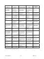
Change Information Page
Title: FRR Document for Cosmic Ray Experiment
Date: 5/23/2005
List of Affected Pages
Page Number
Issue
Date
2
2-15
4-18
18
20-21
Changed some science goals to technical goals
Cosmic ray section added to science goals
Geiger counter section added to science goals
Surface area section added to science goals
Flux section added to science goals and changed flux
formula
Muon section added
Non-vertical section added
Relativistic effects of muons section added
Interaction Depth added
Slant depth added
Second Box design added
HOBO was removed from document
Interfacing recovery edited
Interfacing recovery section fixed
Power budget paragraph added
Mechanical design fixed
Weight Budget error fixed
Sample of software code
Interface board changed to BalloonSAT
Time line error fixed
GAMA-SCOUT® removed from document
Risk Management errors fixed
3/23/05
3/25/05
3/25/05
3/23/05
3/23/05
21-22
23
23-24
24-26
27
30
31
32
33
35
36
37
41
45
49
56-59
56-59
Team CajunSat
ii
3/30/05
4/1/05
4/1/05
4/1/05
4/1/05
3/30/05
4/1/05
4/1/05
4/1/05
4/1/05
4/1/05
4/1/05
4/1/05
4/1/05
4/1/05
4/1/05
4/1/05
FRR v3.0
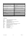
Status of TBDs
TBD
Section
Number
001
002
003
004
005
006
3.1.1
3.1.2
3.1
007
4.2
008
009
010
6.3
4.5
4.5
4.7
4.0
Team CajunSat
Description
Surface area of Geiger Counter tube
Gas in Geiger Counter tube
Time interval for the amount of counts
GPS device actually being used during flight
Resistance of heating circuit
Technical Specs of Geiger-Muller Counter kit
Will a double box provide better results an a
heater.
Dead Time
Geiger counter power
BalloonSAT power
iii
Date
Date
Created Resolved
3/11/05
3/11/05
3/11/05
3/8/05
3/11/05
3/11/05
5/1/05
4/27/05
4/27/05
5/2/05
4/26/05
4/28/05
3/31/05
5/3/05
4/1/05
4/1/05
4/1/05
4/29/05
4/29/05
5/9/05
FRR v3.0
TABLE OF CONTENTS
Cover............................................................................................................................................. i
Change Information Page ............................................................................................................ ii
Status of TBDs ………………………………………………………………………………….iii
Table of Contents........................................................................................................................ iv
List of Figures ...............................................................................................................................v
List of Tables .............................................................................................................................. vi
1.0 Document Purpose ..................................................................................................................1
1.1 Document Scope ...............................................................................................................1
1.2 Change Control and Update Procedures ...........................................................................1
2.0 Reference Documents .............................................................................................................1
3.0 Mission Objectives..................................................................................................................2
3.1 Science Goals....................................................................................................................2
3.1.1 Cosmic Rays ..................................................................................................................3
3.1.2 Muons ..........................................................................................................................17
3.1.3 Non-Vertical Muons ................................................................................................... 18
3.1.4 Interaction Depth .........................................................................................................19
3.1.5 Slant Depth...................................................................................................................22
3.2 Technical Goals ..............................................................................................................22
4.0 Payload Design .....................................................................................................................25
4.1 Principle of Operation.....................................................................................................30
4.2 System Design ................................................................................................................33
4.3 Electrical Design.............................................................................................................34
4.3 Software Design..............................................................................................................36
4.4 Thermal Design...............................................................................................................37
4.5 Mechanical Design..........................................................................................................38
5.0 Payload Development Plan ...................................................................................................47
6.0 Payload Construction Plan....................................................................................................54
6.1 Hardware Fabrication and Testing..................................................................................55
6.2 Integration Plan...............................................................................................................56
6.3 Software Implementation and Verification.....................................................................59
6.4 Flight Certification Testing.............................................................................................85
7.0 Mission Operations ...............................................................................................................67
7.1 Launch Requirements .....................................................................................................68
7.2 Flight Requirements and Operations ..............................................................................68
7.3 Data Acquisition and Analysis Plan ...............................................................................68
8.0 Project Management .............................................................................................................69
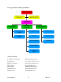
8.1 Organization and Responsibilities ..................................................................................70
8.2 Configuration Management Plan ....................................................................................71
8.3 Interface Control .............................................................................................................71
8.3.1 Electrical Interface .......................................................................................................71
8.3.2 Mechanical Interface....................................................................................................72
8.3.3 Software Interface........................................................................................................72
8.3.4 General Interface..........................................................................................................72
Team CajunSat
iv
FRR v3.0
9.0 Master Schedule....................................................................................................................73
9.1 Work Breakdown Structure (WBS) ................................................................................74
9.2 Staffing Plan....................................................................................................................75
9.3 Timeline and Milestones.................................................................................................76
10.0 Master Budget.....................................................................................................................77
10.1 Expenditure Plan...........................................................................................................78
10.2 Material Acquisition Plan .............................................................................................79
11.0 Risk Management and Contingency ...................................................................................79
11.1 Stress testing .......................................................................................................................87
11.2 Cold testing .........................................................................................................................98
11.3 Vacuum testing ...................................................................................................................99
11.4 Testing of RF emission .......................................................................................................99
11.5 Complete system test of all equipment and in all conditions............................................133
12.0 Glossary ...........................................................................................................................136
Team CajunSat
v
FRR v3.0
LIST OF FIGURES
1. Stopping material of particles .................................................................................................3
2. Victor Hess Flight ...................................................................................................................5
3. Flux of Cosmic Rays...............................................................................................................7
4. Hillas Plot ...............................................................................................................................8
5. Cosmic shower........................................................................................................................9
6. Geiger counter.......................................................................................................................19
7. Geiger counter experiment....................................................................................................21
8. ST-350 pictures.....................................................................................................................26
10. Gamma sensitivity curve.......................................................................................................29
11. LND 7232 Tube ....................................................................................................................29
12. Geiger Plateau.......................................................................................................................31
13. K2645 Geiger Counter..........................................................................................................32
14. Count rate of K2645..............................................................................................................33
15. Schematic drawing of K2645................................................................................................36
16. Environment for payload ......................................................................................................37
17. Dead time experiment ...........................................................................................................39
18. Theoretical flux curve ...........................................................................................................52
19. Muons
.............................................................................................................................53
20. Interaction Depth ..................................................................................................................55
21. Primary cosmic rays interaction............................................................................................59
22. FRED results.........................................................................................................................60
23. Montana University results ...................................................................................................60
24. Outer box diagram ................................................................................................................61
25. Building the outer box ..........................................................................................................62
26. Outer box pictures.................................................................................................................63
27. Inner box diagram .................................................................................................................65
28. Epoxy
.............................................................................................................................66
29. Inner box .............................................................................................................................67
30. Inner box sections .................................................................................................................68
31. Inner box support ..................................................................................................................70
32. System designs......................................................................................................................73
33. Interfacing of systems ...........................................................................................................74
34. Interfacing of recovery..........................................................................................................74
35. Geiger Muller counter...........................................................................................................75
36. Circuit design ........................................................................................................................77
37. Mechanical design ................................................................................................................77
38. Ultra life batteries .................................................................................................................79
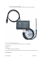
39. VIC-303 scale .......................................................................................................................81
40. Calibration of Scale...............................................................................................................81
41. Weight budget.......................................................................................................................87
42. Wight of each device ............................................................................................................88
43. Flow of construction plan .....................................................................................................92
44. Software .............................................................................................................................95
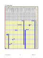
45 Timeline ...........................................................................................................................105
Team CajunSat
vi
FRR v3.0
46. Expenditure plans................................................................................................................107
47. Impact pictures....................................................................................................................109
48. Scientific Workshop............................................................................................................120
49. RTD temperature sensor .....................................................................................................121
50. Voltage sensor ....................................................................................................................122
51. HOBO specifications ..........................................................................................................123
52. Thermal conductivity of single box ....................................................................................126
53. Battery test ..........................................................................................................................127
54. Cold chamber ......................................................................................................................127
55. Vacuum chamber ...............................................................................................................128
56. Oscilloscope .......................................................................................................................133
Team CajunSat
vii
FRR v3.0
LIST OF TABLES
1. Specifications of Spectra ST-350 ..........................................................................................32
2. LND 7232 Geiger Tube General specifications.....................................................................34
3. LND 7232 Geiger Tube Window specifications ...................................................................34
4. LND 7232 Geiger Tube Electrical specifications..................................................................36
5. Dimensions of Geiger counter ................................................................................................37
6. Data from K2645 Geiger counter ..........................................................................................50
7. Muon Interaction density .......................................................................................................57
8. Slant Depth angles ................................................................................................................ 57
9. Requirements of hardware .................................................................................................... 72
10. Power Budget........................................................................................................................80
11. Balance error.........................................................................................................................82
12. Weight budget.......................................................................................................................87
13. Hardware fabrication and testing ..........................................................................................93
14. Organization and responsibilities........................................................................................100
15. Work breakdown structures ................................................................................................103
16. Staffing plan........................................................................................................................104
17. Mater Budget ......................................................................................................................106
18. Purchase record...................................................................................................................108
19. Specifications for Scientific workshop ...............................................................................119
20. RTD specifications..............................................................................................................122
21. Voltage sensor Specifications .............................................................................................122
22. Signal Acquisition system ..................................................................................................129
23. Calibration ranges ...............................................................................................................129
24. Time base systems ..............................................................................................................129
25. Trigger system ....................................................................................................................130
26. Display ...........................................................................................................................130
27. Cursor
...........................................................................................................................131
28. Physical characteristics ...................................................................................................... 131
29. Waveform processes ...........................................................................................................132
30. Non-Volatile stored.............................................................................................................132
31. Option 14: I/O interface ......................................................................................................132
32. Hard copy capabilities.........................................................................................................132
33. Mechanical..........................................................................................................................133
34. Environmental and safety ...................................................................................................133
35. Risk likelihood table ...........................................................................................................134
36. Risk Matrix .........................................................................................................................135
37. Risk solutions......................................................................................................................137
Team CajunSat
viii
FRR v3.0
1.0 Document Purpose
This document describes the critical design for the Cosmic Ray experiment by Team CajunSat
for the ACES Program. It fulfills part of the ACES Program requirements for the Flight
Readiness Review (FRR) to be held May 9, 2005.
1.1 Document Scope
This FRR document specifies the scientific purpose and requirements for the Cosmic Ray
experiment and provides a guideline for the development, operation and cost of this payload
under the ACES Program. The document includes details of the payload design, fabrication,
integration, testing, flight operation, and data analysis. In addition, project management,
timelines, work breakdown, expenditures and risk management is discussed. Finally, the designs
and plans presented here will be finalized at the time when the ACES Program Office approves
this Flight Readiness Review (FRR).
1.2 Change Control and Update Procedures
Changes to this FRR document shall only be made after approval by designated representatives
from Team CajunSat, and the LaACES Program Office. Document change requests should be
sent to Team members, and the LaACES Program Office.
2.0 Reference Documents
1. Mewaldt, R.A. Cosmic Rays. California Institute of Technology. Macmillan
Encyclopedia of Physics 1996. http://www.srl.caltech.edu/personnel/dick/cos_encyc.html
2. Introduction to Ionizing Radiation and Low level Radioactive Materials. Dr. William
Andrew Hollerman, CHMM
3. Cosmic Rays. NASA.
http://imagine.gsfc.nasa.gov/docs/science/know_l2/cosmic_rays.html
http://helios.gsfc.nasa.gov/cosmic.html
http://imagine.gsfc.nasa.gov/docs/science/know_l1/cosmic_rays.html
4. Stanton, Noel. Introduction to Cosmic Rays. July 9, 2003.
http://www.phys.ksu.edu/~evt/Quarknet/Docs/cosmic_ray_intro.pdf
5. http://hyperphysics.phy-astr.gsu.edu/hbase/astro/cosmic.html
6. NASA. COSMICOPIA. http://helios.gsfc.nasa.gov/qa_cr.html
7. Uranium Information Centre Ltd. Nuclear Electricity 7th edition. 2003.
http://www.uic.com.au/neAp1.htm
8. FRED PDR document http://atic.phys.lsu.edu/aces/Teams/2002-2003/FLUX/FLUX.htm
9. FRED CDR document http://atic.phys.lsu.edu/aces/Teams/2002-2003/FLUX/FLUX.htm
10. HOBO
http://www.onsetcomp.com/Products/Product_Pages/HOBO_H08/H08_family_data_logg
ers.html#Anchor-HOBO-23240
11. http://www.aboutnuclear.org/view.cgi?fC=Radiation_and_Radioactivity,Types_of_Radia
tion
Team CajunSat
1
FRR v3.0
12. Student Ballooning for Aerospace Workforce Development. Guzik T.G. and J.P. Wefel.
Louisiana State University. August 9, 2004
13. Phillips, Tony. Ballooning for Cosmic Rays.
http://www.firstscience.com/site/articles/balloon.asp
14. University of Leeds. What are Cosmic Rays?
http://www.ast.leeds.ac.uk/haverah/cosrays.shtml
15. How a Geiger Counter works. http://nstg.nevada.edu/PAHRUMP/handoutcont2.html
16. http://polaris.phys.ualberta.ca/info/Phys29x/Manual/11GM01.pdf
17. Muons. http://www.lbl.gov/abc/cosmic/SKliewer/Cosmic_Rays/Muons.htm
18. Interaction Depth http://www.lbl.gov/abc/cosmic/SKliewer/Cosmic_Rays/Interaction.htm
19. http://www.answers.com/topic/geiger-mueller-tube
3.0 Mission Objectives
The mission objective of this experiment is to measure the flux of the secondary cosmic rays
with respect to altitude.
3.1 Science Goals
The scientific goal of this experiment is to measure the total cosmic ray flux, or rate of flow of
radiation per unit area, of the cosmic rays in the atmosphere with respect to altitude. However,
this will not be a total flux because we do not expect to detect any alpha particles. This is
because alpha particles are stopped by a piece of paper. Therefore our two layers of foam board
will stop all alpha particles. Beta particles and gamma rays, on the other hand, will not be
stopped by the foam board because beta rays are stopped by a sheet of aluminum or plywood
while gamma rays are stopped by a two meters of concrete or 40 cm of lead (Reference 11)
Figure 3.1 shows this better.
Team CajunSat
2
FRR v3.0
Figure 3.1
This shows how far each particle can travel through a given object.
http://www.cameco.com/uranium_101/uranium_science/radiation/index.php
3.1.1 Cosmic Rays
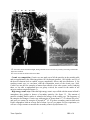
Cosmic rays are particles that bombard Earth from anywhere beyond its atmosphere
(Reference 3) and were discovered by Victor Hess (see figure 3.2) using a high altitude balloon
traveling to about 17,500 feet (5.334 km) and a gold leaf electroscope (Reference 14). He
noticed that the electroscope discharged more rapidly has we went up in altitude and attributed
this as a form of radiation entering the atmosphere from above. This discovery earned him a
Nobel Prize in 1936. For a long time, cosmic rays were considered electromagnetic in nature, but
during the 1930’s it was discovered that they are electrically charged and affected by things such
as Earth’s magnetic fields. This means that the flux of the cosmic rays will be different at
different latitudes and at different altitudes because Earth acts like a bar magnet. This also means
that it is impossible to tell the exact origin of the cosmic rays (Reference 1).
Early Research: During the 1930’s to 1950’s, man-made particle accelerators were unable to
reach very high energies so cosmic rays served as a source of particles for high energy physics
which led to the discovery of the first muon and pion. However, this is not the only application
of comic rays. In fact, since the beginning of the space age, the main focus of cosmic ray
research has been towards astrophysical investigations of where cosmic rays originate, how they
get accelerated to such high velocities, what role they play in the dynamics of the Galaxy, and
what their composition tells us about matter from outside our solar system. In order for us to
measure cosmic rays directly, we must do our research on space craft and high altitude balloons
before they have a chance to be broken up and slowed down by Earth’s atmosphere (Reference
1).
Cosmic Ray energies and Acceleration: Cosmic rays are usually measured in units of MeV
or GeV, and their energy range is a little less than 1 MeV to a little over 1 ZeV (1021 eV) which
is about one billion times more powerful than any current particle accelerator (See Figure 3.2).
Team CajunSat
3
FRR v3.0
Most galactic cosmic rays have an energy range of 100MeV to 10GeV or a velocity range of
46% to 99.5% the speed of light. The number of cosmic rays with energies above 1 GeV
decreases by a factor of 50 for every factor of 10 increase in energy. The highest energy rays
measured to date is 1020 eV (Reference 1).
It is believed that most galactic cosmic rays derive their energy from supernova explosions,
which occur approximately once every 50 years in our galaxy. For cosmic rays to maintain their
intensity over millions of years requires only a few percent of the 1044 J released by the typical
supernova explosion. There is also evidence that cosmic rays are accelerated as the shock waves
from these explosions traveling through interstellar gas. The energy contributed to the Galaxy by
comic rays is about that contained in galactic magnetic fields, and in the thermal energy of the
gas that passes through the space between the stars. This is approximately 1 eV per cm3
(Reference 1).
While we might be able to detect cosmic ray energies, we do not always know how they are
accelerated to such a high velocity. In fact, the source of energy greater than 1015 eV is unknown.
It is believed that they might originate from outside our galaxy from active galactic nuclei,
quasars, or gamma ray bursts, but it can also be some exotic new physics such as superstrings,
exotic dark matter, strongly-interacting neutrinos, or topological defects in the very structure in
the universe (Reference 3).To better see this, see figures 3.2 and 3.3.
Team CajunSat
4
FRR v3.0
Figure 3.2.
Left: Victor Hess before his balloon flight, during which he observed cosmic ray intensity increasing with altitude.
Right: Hess's balloon.
http://www.ast.leeds.ac.uk/haverah/cosrays.shtml
Cosmic ray composition: Cosmic rays are made out of all the particles in the periodic table
and are approximately the following portion: 89% hydrogen (protons), 10% helium, and 1% of
the heavier elements such as carbon, oxygen, magnesium, silicon, and iron (Reference 1). By
studying cosmic rays, we can know what the composition source of the cosmic rays. Also,
Cosmic rays are the few examples of matter from outside of our solar system, and by studying
them, we are able to understand how our galaxy evolved, the reason for the matter in our
universe, and our origin (Reference 3).
High energy cosmic rays: When the high energy cosmic rays collide with the atoms in Earth’s
atmosphere, they produce a shower of secondary particles. See figure 3.5. The amount of
particles reaching Earth’s surface is related to the energy of the cosmic rays. The frequency of
the energies also changes. Cosmic rays with energies of greater than 1015 eV is about 100 per m2
and once per century for energies of beyond 1020 eV. It is these secondary particles that reach
Earth’s atmosphere with an average flux of about 1 per m2 per minute. For our experiment, we
will use a Geiger counter to measure the secondary cosmic rays (Reference 14).
Team CajunSat
5
FRR v3.0
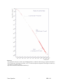
Figure 3.3
This graph shows the flux of cosmic rays bombarding Earth as a function of their energy per particle. Researchers
believe cosmic rays with energies less than ~3x1015 eV come from supernova explosions. The origin of cosmic rays
greater than 1015 remains a mystery.
http://www.firstscience.com/site/articles/balloon.asp
Team CajunSat
6
FRR v3.0
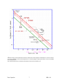
Figure 3.4
Hillas Plot. Red, green and dotted lines show the relation between the magnetic field and the size of an accelerator.
Once energy and charge of the accelerated particle are fixed Astrophysics objects placed above a line are candidate
sites for acceleration.
http://etd.adm.unipi.it/theses/available/etd-06142004-215416/unrestricted/ch1.pdf
Team CajunSat
7
FRR v3.0
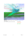
Figure 3.5 A
This is a computer simulation of the primary cosmic rays interacting
with the atmosphere.
http://www.th.physik.uni-frankfurt.de/~drescher/CASSIM/
Team CajunSat
8
blue: electrons/positrons
cyan: photons
red: neutrons
orange: protons
gray: mesons
green: muons
FRR v3.0
Figure 3.5 B
This is a computer simulation of the primary cosmic rays interacting
with the atmosphere.
http://www.th.physik.uni-frankfurt.de/~drescher/CASSIM/
Team CajunSat
9
blue: electrons/positrons
cyan: photons
red: neutrons
orange: protons
gray: mesons
green: muons
FRR v3.0
Figure 3.5 C
This is a computer simulation of the primary cosmic rays interacting
with the atmosphere.
http://www.th.physik.uni-frankfurt.de/~drescher/CASSIM/
Team CajunSat
10
blue: electrons/positrons
cyan: photons
red: neutrons
orange: protons
gray: mesons
green: muons
FRR v3.0
Figure 3.5 D
This is a computer simulation of the primary cosmic rays interacting
with the atmosphere.
http://www.th.physik.uni-frankfurt.de/~drescher/CASSIM/
Team CajunSat
11
blue: electrons/positrons
cyan: photons
red: neutrons
orange: protons
gray: mesons
green: muons
FRR v3.0
Figure 3.5 E
This is a computer simulation of the primary cosmic rays interacting
with the atmosphere.
http://www.th.physik.uni-frankfurt.de/~drescher/CASSIM/
Team CajunSat
12
blue: electrons/positrons
cyan: photons
red: neutrons
orange: protons
gray: mesons
green: muons
FRR v3.0
Figure 3.5 F
This is a computer simulation of the primary cosmic rays interacting
with the atmosphere.
http://www.th.physik.uni-frankfurt.de/~drescher/CASSIM/
Team CajunSat
13
blue: electrons/positrons
cyan: photons
red: neutrons
orange: protons
gray: mesons
green: muons
FRR v3.0
Figure 3.5 G
This is a computer simulation of the primary cosmic rays interacting
with the atmosphere.
http://www.th.physik.uni-frankfurt.de/~drescher/CASSIM/
Team CajunSat
14
blue: electrons/positrons
cyan: photons
red: neutrons
orange: protons
gray: mesons
green: muons
FRR v3.0
Figure 3.5 H
This is a horizontal view of the secondary cosmic ray shower.
http://www.th.physik.uni-frankfurt.de/~drescher/CASSIM/
Team CajunSat
15
blue: electrons/positrons
cyan: photons
red: neutrons
orange: protons
gray: mesons
green: muons
FRR v3.0
Figure 3.5 I
This is a vertical view of the secondary cosmic ray shower.
http://www.th.physik.uni-frankfurt.de/~drescher/CASSIM/
Team CajunSat
16
blue: electrons/positrons
cyan: photons
red: neutrons
orange: protons
gray: mesons
green: muons
FRR v3.0
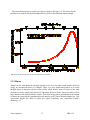
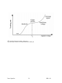
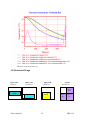
This interaction of primary cosmic rays causes a graph as in Figure 3.6. The reason for the
peak has to do with the interaction length which is given by the following muon example.
Figure 3.6
This shows the theoretical curve of the flux with respect to altitude.
3.1.2 Muons
Muons are the most numerous charged particles at sea level. In other words, muons must lose
energy by ionization because it is charged. There is no way around this because as it passes
through matter it interacts with the electric fields which knocks loose off some of the outer
electrons; however, muons only interact by ionization. Because of this, muons are able to travel
large distances and reach the Earth’s surface. Their only energy lost is proportional to the amount
of matter they pass which is proportional to the density (g/cm3) times the path length (cm). This
"interaction length" has units of grams per square centimeter (see “Interaction Depth”)
(Reference 17).
Team CajunSat
17
FRR v3.0
Figure 3.7
This graph just shows the primary cosmic rays entering Earth’s
atmosphere and creating muons.
http://www.lbl.gov/abc/cosmic/SKliewer/Cosmic_Rays/Muons.htm
The Muon energy lost is a constant rate of about 2 MeV per g/cm2. Since the vertical depth of
the atmosphere is about 1000 g/cm2, muons will lose about 2 GeV to ionization before reaching
the ground. The mean energy of muons at sea level is still 4 GeV. Therefore the average energy
at creation is approximately about 6 GeV (Reference 17).
The atmosphere is so weak at higher altitudes that even at 15 km it is still only 175 g/cm2 deep.
Typically, it is about here that most muons are generated and also the peak of the flux of the
cosmic rays. The average muon flux at sea level is 1 muon per square centimeter per minute.
This is about half of the typical total natural radiation background (Reference 17).
Muons (and other particles) are generated within a cone-shaped shower, with all particles
staying within about 1 degree of the primary particle's path (Reference 17).
3.1.3 Non-Vertical Muons
Muons arriving at some angle θ from the vertical will have traveled a path length that increases
as 1/cos (θ). (See "Slant Depth") This assumes that the Earth is essentially flat (less than 1%
error for θ < 70°) and that muons do not decay over the extended path length (Reference 17.
Team CajunSat
18
FRR v3.0
If we assume that twice the path length would attenuate the muons to half as many, then we
would expect the muon flux to vary as the cos (θ). However, the observed distribution is
proportional to cos2 (θ). This is a difference of less than 10% at an angle of 27° and 20% at 43°.
This difference may be primarily due to the approaching decays of muons, as the path length
exceeds their range (Reference 18).
3.1.4 Interaction Depth
The energy of charged particles is progressively absorbed by ionizing the matter it passes
through. The greater the matter and the greater the distance, the more absorption. Cosmic rays
pass through a great variety of environments, from the almost absolute emptiness of extragalactic
space to the relative mess of our atmosphere, to the extreme density of our Earth or even lead
shielding. We need to measure the path length that would help us predict the absorption. At any
point along the path, the number of interactions is proportional to the density (r) times the path
length (dr). If we were to add up all of these interactions along the particle's path, we would get a
number that should be proportional to the total absorption (Reference 18).
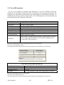
If density has units of g/cm3 and the path length is in units of cm, then this Interaction Depth,
X, has units of g/cm2. At first it seems strange to be talking about some sort of distance with
units of g/cm2, but it does allow us to compare the effects of passage through kilometers of the
upper atmosphere, to passage through a few centimeters of water (Reference 18).
Figure 3.9
This Picture shows that different angles that the can be formed when the
primary cosmic rays reach Earth.
http://www.lbl.gov/abc/cosmic/SKliewer/Cosmic_Rays/Interaction.htm
The pressure here at the surface of the earth, although partly due to dynamic effects of air
movement, is mostly due to the total weight of the air above that point. The cross-sectional area
of a column of air radiating directly upward, gets larger as it rises. The acceleration of gravity
decreases as you get farther away. However, the earth is so large and the atmosphere so thin, that
both of these values are essentially constant (to within 1%) (Reference 18).
Team CajunSat
19
FRR v3.0
Thus at some altitude h, the pressure divided by g (=9.8m/s2) is a measure of the absorption
along a vertical path to that point. The 1967 Standard Atmosphere (see article later) gives us
empirical equations to calculate the pressure at any altitude. The standard atmospheric pressure
at sea level is defined as 101,325 Pa. The “depth” X, is therefore equal to ~10,000 kg/m2 or 1000
g/cm2. As divers know, a depth of 10 meters in water (density = 1 g/cm3) provides an additional
atmosphere of pressure. In other words 10 meters of water will provide the same absorption as
the entire thickness of the atmosphere (Reference 18).
Team CajunSat
20
FRR v3.0
Material
Density
(g/cm3)
Thickness
1 Atm. Equivalent
Interstellar Space
10-23
100 million LY
Air at 15,000 m (muon production zone)
0.00019
53,000 m
Air at 12,500 m (max. KAO experiment)
0.00029
34,000 m
Air at 4,000 m (Top of Mauna Kea)
0.00082
12,000 m
Sea Level Air
0.00125
8,000 m
Water
1
10 m
Rock
5
2m
Iron
8
1.3 m
Lead
11
0.9 m
Table 3.1
This chart shows different materials with their densities and their equivalent to 1 atmospheric pressure.
http://www.lbl.gov/abc/cosmic/SKliewer/Cosmic_Rays/Interaction.htm
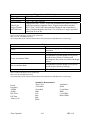
Altitude
ft
Note
m
Density
Pressure
Depth
g/cm3
Pa
g/cm2
233,000
71,000
Top of Std Atmosphere
6x10-8
67
0.7
105,000
32,000
Halfway
1x10-6
868
9
49,000
15,000
Zone of Muon production
2x10-4
12,000
130
41,000
12,500
Max. alt. KAO experiment
3x10-4
18,000
180
36,000
11,000
4x10-4
23,000
230
13,000
4,000
Top of Mauna Kea
8x10-4
62,000
630
0
0
Sea Level
1x10-3
101,000
1,000
Table 3.2
This chart shows different altitudes with their density, pressure, and depth.
http://www.lbl.gov/abc/cosmic/SKliewer/Cosmic_Rays/Interaction.htm
Team CajunSat
21
FRR v3.0
3.1.5 Slant Depth
All of the above Depth calculations are true only for muons arriving vertically. By simple
trigonometry, it can be seen that dr' (distance along the slanted path) is equal to dr / cos (θ) where
θ is the angle of the path measured from vertical (Reference 18).
Given a slant depth, we can use the standard atmosphere pressure equation to extrapolate an
equivalent altitude that would correspond with this depth if it were vertical. This will allow us,
using ground level measurements, to extrapolate the muon intensity vs. altitude graph from the
KAO experiment to negative altitudes (i.e. below sea level) (Reference 18).
In the following table: X' = X / cos (θ), The Equivalent Altitude uses the 1st layer pressure
equation from the standard atmosphere model. The last three columns are provided as a
comparison to the observed cos2 distribution to which the particle data book refers. The
discrepancy is most likely due to muon decays (Reference 18).
θ
Slant Depth, X'
(g/cm2)
Equiv. Altitude
(m)
X0 /cos2 (θ)
(g/cm2)
cos2 (θ)
cos (θ)
0°
1,034
0
1,034
1
1
15 °
1,070
-293
1,108
0.966
0.933
30 °
1,194
-1230
1,378
0.866
0.750
45 °
1,462
-3,022
2,068
0.707
0.500
60 °
2,068
-6,249
4,135
0.500
0.250
75 °
3,994
-13,000
15,432
0.259
0.067
Table 3.3
This graph shows the various angles.
http://www.lbl.gov/abc/cosmic/SKliewer/Cosmic Rays/Interaction.htm
All of the following sections on Muons explained in depth the interaction length of cosmic rays
and gave some examples of each.
3.2 Technical Goals
Our technical goals are as follows:
1.
Accurately measure the total flux of the cosmic rays with respect top altitude.
2.
Obtain knowledge of sensors, electronics, and systems
3.
Learn how to develop and maintain a research program
4.
Learn how to create different environmental simulation testing
5.
Have a successful flight
6.
Obtain useful accurate information
Team CajunSat
22
FRR v3.0
The major technical goal of this experiment is to accurately measure the total flux of the
cosmic rays with respect to altitude. We also expect to get a graph that will look similar to Figure
3.2. To do this, we must keep the temperature to no less than -20 °C because that is minimal
operating range. To do this, we will be using a heating circuit that should keep the temperature to
above 0 °C.
Figure 3.10
Graph showing the shower of secondary cosmic rays.
http://hyperphysics.phy-astr.gsu.edu/hbase/astro/cosmic.html
Team CajunSat
23
FRR v3.0
Figure 3.11
Expected results, according to FRED experiment performed by LSU team
Figure 3.12
This is another cosmic ray experiment. It was performed on FLIGHT#: BOR0109A by the Montana High Altitude
balloon program.
http://spacegrant.montana.edu/borealis/missions/BOR0109A/index.php
Team CajunSat
24
FRR v3.0
4.0 Payload Design
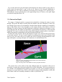
Figure 4.1
This is the outer box which will house our inner box. This box will
also have a switch on the outside running from the BalloonSAT to
outside the box. This is for us to be able to turn on the BalloonSAT just
before launch to conserve battery power.
Team CajunSat
25
FRR v3.0
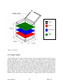
Heaters
Batteries
BalloonSAT
Geiger
counter
Figure 4.2
Diagram of our inner box.
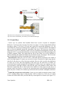
4.1.1 Geiger Counter
The first thing that we need to calculate the flux is the amount of particles (counts) at a given
altitude. To get this, we will use a Geiger counter, which according to Webster is an instrument
for detecting the presence and intensity of radiations (as cosmic rays or particles from a
radioactive substance) by means of the ionizing effect on an enclosed gas which results in a pulse
that is amplified and fed to a device giving a visible or audible indication. The exact gas varies
for each detector, but it always includes a mixture of gases. This mixture always includes an inert
gas, usually neon or argon, and organic vapor such as halogen or alcohol vapor. (Reference 19)
The Geiger counter we will be using is the Geiger Muller Counter - Nuclear Radiation Detector
K2645. This Geiger counter like every other Geiger counter consists of two basic parts: the probe
and the counter. The probe is filled with a gas with a wire down the middle that measures the
radiation. This probe has two primary functions: keeping track of how much radiation is
Team CajunSat
26
FRR v3.0
detected by means of a counting circuit and to provide power for every component on the Geiger
counter. (Reference 14)
Once power is supplied to the probe, a large potential is created making the central wire
become the anode, and the metal wall becomes the cathode. At this stage, the gas is neutral until
radiation enters the probe creating a shower of particles inside the tube. This shower knocks off
electrons creating both free electrons and gas ions which force the electrons to be pulled off
rapidly to the central wire. Once this happens, the electrons are collected on the wire are sent
through the wire into the counting circuit which measures the current. As this process occurs, the
gas ions are slowly building up around the outer wall of the probe which forms a “sheath”. This
reduces the potential and stops the cascade of secondary particles. Once the cascade has ended,
the ions and electrons recombine to form the neutral gas atoms again. This process, called
quenching, and serves to “reset” the detector, allowing it to detect another radioactive emission.
This cycle of the first ionization to the resetting is referred to as the dead time and is typically
100 to 300 microseconds. To get a better picture of this, see Figure 3.6 (Reference 14).
Another thing that we must figure out for the Geiger counter to operate effectively is the
Geiger plateau. If the voltage is too low, the passage of radiation into the tube will not cause a
voltage pulse. The characteristic curve for any tube is obtained by graphing the counting rate
verses the applied voltage. This curve is shows in Figure 4.3. The counting rate C is the number
of counts N registered by the tube divided by the counting time T. The region where the number
of counts is approximately linear and changes little with voltage is called the Geiger plateau. To
preserve the life of the tube, the operating voltage is generally selected within the initial 1/3 of
the plateau. We will find this plateau for our calibration Geiger counter by placing a radioactive
source and adjusting the voltage. Afterwards, we will graph our data and determine the
appropriate operating voltage. The exact procedures used to obtain the graph in Figure 3.8. was
designed by the University of Louisiana at Lafayette physics department for the Modern Lab.
We will not be able to find the Geiger plateau for the K2645 Geiger counter. Therefore, the
plateau will only be used to ensure that our calibration detector is operating correctly. Once we
have determined this, we will measure the flux of both Geiger counters, with the same source
from the same distance, and compare the results.
After doing this, we will find the dead time of each Geiger counter. Once we find the dead
time, we will compare the flux of each Geiger counter. The dead time procedures will be
explained in a later section. After we complete all of this, we will know that the K2645 is
operating correctly.
Team CajunSat
27
FRR v3.0
Figure 4.3.
This shows how exactly a Geiger counter works.
http://nstg.nevada.edu/PAHRUMP/Microsoft%20PowerPoint%20-%20Geiger%20Counter%20Diagrams.pdf
Team CajunSat
28
FRR v3.0
Figure 3.7
This is the theoretical Geiger counter voltage curve.
http://polaris.phys.ualberta.ca/info/Phys29x/Manual/11GM01.pdf
Team CajunSat
29
FRR v3.0
4.1 Principle of Operation
The Geiger-Muller Counter will measure the flux of cosmic rays in counts per minute. This
counter will be interfaced with the BASIC Stamp, sending data to the EEPROM of the BASIC
stamp. Temperature measurements will be collected throughout flight and stored into the BASIC
stamp. These measurements will be used to determine that the electronics remained in operating
temperature range (-20 ºC – 70 ºC). To maintain this temperature there will be two heating
circuits inside the payload as noted in the above figure 4.1. If a particular section of collected
data seems inaccurate, we can reference our temperature data for a plausible cause of the
inaccuracy. After flight using pre-tested software, the data will be dumped from the EEPROM of
the BASIC Stamp. The goal of our payload is to combine the collected data from flight, and the
tracking team’s data to produce a final graph of the intensity of cosmic rays in flux with respect
to altitude as described in section 3.0.
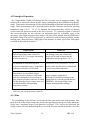
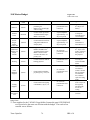
Hardware
Requirements
Internal temperature must remain at a
minimum of -20 ºC for proper functioning
of electrical devices
One heating circuit and a double box
design will be used to ensure that the
temperature does not go below -20°C.
To determine if electronics stayed in
necessary temperature range. Temperature
readings are needed to be collected
Thermistors on the BalloonSAT will be
used to make sure that we have maintained
a correct operating temperature.
Data needs to be stored from Geiger
Counter in order to analyze results in the
end, also a timing device is necessary to
keep accurate accounts of the time in which
the data from the Geiger counter came so it
can match with the corresponding
temperature reading.
BASIC Stamp is connected to
BalloonSAT, which has a timing circuit
already built in, is inside payload and two
EEPROM’s for storage of the Geiger
Counter and temperature readings
Fig 4.2
Table of the flow from Requirements to Hardware
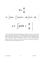
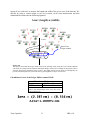
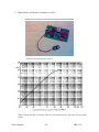
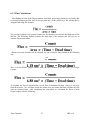
4.1.2 Flux
The second thing we need to know to calculate the flux is the surface area of the detector. This
turns out to be really simple because the particles are traveling near the speed of light making the
Geiger tube a stationary target for the particles (see Figure 3.18). Also for the most part, the
Geiger counter will only rotation along the xy-axis with very little motion around the z-axis This
Team CajunSat
30
FRR v3.0
means all we need to do is measure the length and width of the active area of the detector. We
did this by using a vernier caliper to get very accurate (±0.05 mm) measurement and then
substituted the results into the following equation:
Area= (length) x (width)
γ
γ
γ
γ
γ
γ
γ
γ
γ
γ
z-axis
γ
γ
γ
γ
γ
γ
γ
γ
γ
Area of our
Geiger counter
γ
Geiger tube
Figure 3.18
This picture shows that the Geiger counter tube will be spinning mostly along the z-axis and the radiation
will mostly be coming from the top down making the Geiger counter area a rectangle to the particles. This is
shown by the blue box around the Geiger counter. Also alpha particles are not shown even though they are
present in the atmosphere they will not be able to get through the two layers of foam core.
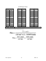
Calculations of Area of the Geiger Muller counter K2645
Dimensions of Geiger counter
Length
2.287 cm ± 0.05 mm
Width
0.516 cm ± 0.05 mm
Table 3.6
This is our measurements of the active area of the
Geiger Muller tube.
Area=1.180092 cm2
Team CajunSat
31
FRR v3.0
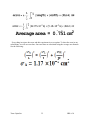
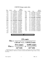
Average area = 0.751 cm2
Every thing in science has error and this experiment is no exception. To show the error in our
calculations, we will use error bars. Our error bars are calculated using the average area formula.
See the following:
Team CajunSat
32
FRR v3.0
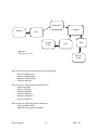
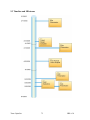
4.2 System Design
Data Storage
Thermistor
Switch
Battery
Battery
BalloonSAT board
Geiger-Muller
Counter
Heater
Data Storage
Fig 4.3
Major Components of payload
Resistors
Batteries
Heating
Circuit
BalloonSAT
Board
Geiger-Muller
counter
Switch
Team CajunSat
Batteries
33
Figure 4.4
Interfacing of systems
FRR v3.0
BalloonSAT
Balloon
Computer
Box
Ground
Team
GPS
Data
Figure 4.5
Interfacing of recovery
Results/
Graph
There will be electrical interfacing between the following:
- Geiger to BalloonSAT
- Heaters to BalloonSAT
- Batteries to BalloonSAT
- Switch to batteries
There will be the following Structural Interfaces
- Board to payload
- Geiger to payload
- Heaters to payload
- Switch to payload
- Batteries to payload
- Payload to Balloon
There will be the following software Interfaces
- Geiger to BalloonSAT
- BalloonSAT to personal computer
Team CajunSat
34
FRR v3.0
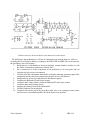
4.3 Electrical Design
G-M tube
Output to
BalloonSat board
Figure 4.6 A
Geiger-Mueller counter schematics
The modification in order to couple with BalloonSAT board is shown.
VCC
VCC
U3
U2
+5V
+9V
VIN
VDC
SCL
6
P9
SDA
5
P8
to U1
U1
From Geiger Counter
100K
1
SOUT
VIN
2
SIN
VSS
3
ATN
RES
4
VSS
VDD
5
P0
P15
6
P1
P14
7
P2
P13
8
P3
P12
9
P4
P11
P5
P10
P6
P9
P7
P8
10
11
100K
12
24
23
VCC
22
21
20
19
18
17
16
15
14
13
SCL
to U2
SDA
U1 – BASIC Stamp Microcontroller (BS2P24)
U2 – EEPROM Memory (24LC64)
U3 – Power regulator
Figure 4.6 B
Interfacing BASIC Stamp with Geiger Counter Kit
Team CajunSat
35
FRR v3.0
Notations correspond to the ones used in “BalloonSAT Assembly Manual”
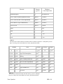
Power Budget
Component
BalloonSAT
and 9V
Geiger Counter
Batteries
9V
Voltage
Current
Low :0.04 A
High: 0.06 A
1.8 A
Power
Low: 0.36 W
High: 0.54 W
11.7 W
Table 4.1
This is our power budget table for the flight. There are two lithium batteries being used. One is for the Geiger
counter and the other one is for the BalloonSAT and heater.
The power supply of the payload will consist of three 9V lithium batteries. One battery will be
supply the Geiger counter and the Interface board while the other battery will provide power to
the other electrical units. The complete interfacing design can be viewed in figures 4.3, 4.4, and
4.5. There will be four main electrical components, heating circuits described thoroughly in
section 4.4 and figures 4.7a, and 4.7b. This circuit will consist of a 0.5 W ceramic resistor and
there will be two of them located within the payload. Temperature data will be stored with the
BASIC stamp and its memory on the BalloonSAT board. The final two components are the
Geiger counter and the Interface Board which will be interfaced together, reference to figure 4.6
for the interfacing schematics. This interfacing is described as follows:
The CD4040 is used to count the Geiger ticks. The clock input is connected to the middle of
two series 100 K resistors. One of the resistors is connected to ground and the other is connected
to pin four of IC U1 (the CD40106 or 74C14) on the Geiger counter. The Stamp will be powered
from the same 9V battery as the Geiger counter. The 74C157 data selector allows the stamp to
read 8 bits of the counter, one nibble at a time. The 9th bit is read by the stamp. All other bits are
discarded, allowing up to 512 counts in a one minute period. The A/B selector on the 74C157
doubles as a serial output for the PC interface. The Geiger counter reading is updated once per
minute and is based on the total counts received -- from between one minute, and four hours of
operation. The longer the device is operated, the more accurate the readings will be. The Stamp
sends the minute-by-minute reading out as numeric data, followed by a carriage return and line
feed at 2400 Baud. When the Stamp is turned on, this data is immediately sent out through the
serial port at 2400 Baud. The data is sent numerically with a line feed and carriage return after
each number, the earliest measurement first.
Team CajunSat
36
FRR v3.0
Ceramic
Resister
Resistance
20 Ώ
__
9V
Wires
+
Battery
Figure 4.7 a
Circuit design of Heating Circuit
Figure 4.7 b
The heating Circuit design
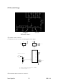
4.4 Thermal Design
We expect to encounter an environment with temperatures ranging from -60 ºC to 80 ºC. The
electrical components in our payload (BASIC stamp, Geiger counter, etc) have operating ranges
of minimum -20 ºC to maximum 70 ºC. The only problem this causes is maintaining the
payloads temperature at -20 ºC at max altitude, and min pressure. If temperature is not
maintained at this level then collected data can become inaccurate, and not sensible. We are
going to use two simple heating circuits figure 4.7a, and 4.7b to maintain temperature at
operating level. The only temperature dependencies will be remaining in operating temperature
range in order to collect valid data.
Team CajunSat
37
FRR v3.0
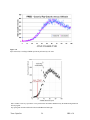
Figure 4.8
This is the results of our heater test.
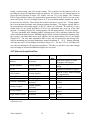
4.5 Mechanical Design
Figure 4.8A
Top level
Geiger
Counter
Team CajunSat
Figure 4.8 A
second level
Figure 4.8B
third level
Fig 4.8 C
bottom level
Battery
three
Heating
Circuit
BalloonSAT
38
Battery
one
Battery
two
FRR v3.0
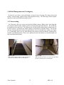
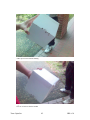
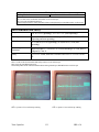
Figure 4.2 A
Robert Moore building the outside box. Mask is used because of the fumes of the epoxy.
Figure 4.2 B
Picture of the outer box.
Team CajunSat
39
FRR v3.0
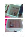
Figure 4.2C
This is a picture of the inner box.
See figures 4.1, and 4.3 for a complete picture of the payload. It will contain on the bottom the
Geiger counter, and BalloonSAT figure 4.10a, there will be a heating unit.. On the front face
three 9 V batteries will be mounted figure 4.10d. Multiple stress test will be performed in the
near future for determination of best mounting method for devices inside payload. The
interfacing of interior parts of the payload can be examined in Figure 4.4a, and 4.4b.
The payload box will be a 15 cm by 15 cm by 15 cm cube box made out of foam board and
possibly a second foam board 13 cm by 13 cm by 13 cm. This will be so that we can not have to
use a heater eliminating weight. The components will be properly sealed and cushioned in order
to withstand the unpredictable flight and landing. The landing could be rough but all we need to
recover out of the payload is the memory chip off of the BASIC Stamp. Our weight budget was
450 g.
The battery we are using for all devices is a 9V Lithium Ultra life Longest life battery. The
specifications on it are as follows:
Team CajunSat
40
FRR v3.0
Team CajunSat
41
FRR v3.0
The scale we are using is VIC-303 0.001g Precision Balance with the following features:
•
•
•
•
•
•
•
•
•
•
•
•
4 models with milligram readability
Protective flip-down and removable plastic cover for shipping protection and allows
stackable storage
Integrated external calibration weights
Unique durable design for all applications
Applications include: Counting, Percent Weighing, Totaling, Display Hold, Specific
Gravity, Mass unit conversion
14 Mass unit conversions (g, oz, lbs, lbs: oz, dwt, ozt, grains, Newton, carats, Taels
HK/Taiwan/Singapore/China, user defined)
Optional RS-232 or USB interface kit (field installable)
Parts counting with selectable reference sample (1-100)
Included AC adapter
External one button calibration with 3 weight options
Lock down capability
Two year manufacturer warranty
Team CajunSat
42
FRR v3.0
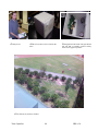
Figure 4.9
Picture of the scale we are using.
http://www.acculab.com/products/
Figure 4.10
Picture of us actually weighing the box.
Team CajunSat
43
FRR v3.0
Calibrations for Balance
To calibrate the weight and get the error we did the following:
1. Put our balance on a level surface.
2. Zero it out
3. Use Fisher #540300 Brass weight set of various weights
4. Use 2 measurements of the weights to get an average error
5. The following is a list of the error:
Weight
Error
±0.014 g
±0.019 g
±0.006 g
±0.004 g
200 g
100 g
050 g
020 g
Table 4.2
Average area of the weights.
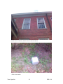
Figure 4.11
This one 200 g weight being used to calculate the error of the balance.
Measuring procedures are as follows:
If the weight is less than 300 g we will use the VIC-303 0.001 g Precision Balance and
the following procedures:
1.
2.
3.
4.
Make sure balance is level
Zero out the balance
Place the object to weighed on the balance
Weight until the balance comes go a general number within to about 0.020 g. We
cannot get an exact number because it will continue to fluctuate by about ±0.020g
because of environment. We just add this fluctuation to the error with the balance
error.
Team CajunSat
44
FRR v3.0
5. Take a picture of the weight to used as documentation
6. Record the weight
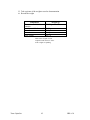
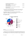
Component
Electronics with 3 lithium
batteries
Inner box with balsa wood
Outer box
Foam inserts
Total weight
Weight (g)
225.56 g
90.10 g
89.8 g
12.0 g
446.5 g
Table 4.3
Table of the weights of each
component with the error. Some
of the weights are pending.
Team CajunSat
45
FRR v3.0
Figure 4.14
Weight Budget Breakdown
Team CajunSat
46
FRR v3.0
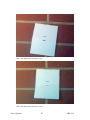
Figure 4.12 A
Weight of our outer box.
5.0 Payload Development Plan
The design for the circuitry involved is complete except for two major points. We still need to
do environmental testing for several components and we need to calibrate the Geiger counter.
Environmental testing requirements for the flight are -60 ºC and 7.6 Torr. Both of these are
approximations based on standard models and previous measurements.
All environment tests are complete except for the heaters and Geiger-Muller counter. The
heating problem can only be resolved by prototyping. The question to address is how sufficient is
a single 1 W ceramic resistor. This will be accomplished by performing the same environmental
testing as for all other components. Both of these points are critical in determining the number of
batteries needed for the payload and ultimately final payload mass.
The only other design issue is determining the accuracy of the Geiger counter. This will be
accomplished by testing the counter against known gamma sources and calculating the flux at
sea level and comparing it to the known flux.
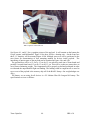
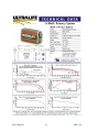
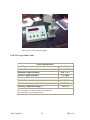
5.1.1 Geiger Muller Counter K2645
The Geiger counter we will be using is the Geiger Muller counter K2645 kit created by
Velleman® Inc. This kit provides an acoustic measurement of radiation levels. The sensitivity is
at its highest for gamma rays and high energy beta rays. The assembly is compact and may be
mounted into a small box, together with the 9V-battery. The specifications are as follows:
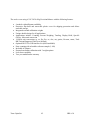
1.
2.
3.
4.
Battery supply of 9V
Maximum current of 200 µA.
Sensitive to gamma-rays and high-energy beta-rays
Dimensions are 54 x 99 x 25 mm
Team CajunSat
47
FRR v3.0
5. Characteristics of tube have a tolerance of ±10%.
Figure 3.14
Picture of our completed Geiger counter.
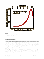
Figure 3.15
Graph of typical count rate as a function of dose rate from Cobalt-60 source. This comes from the product
manual.
Team CajunSat
48
FRR v3.0
Comparing the gamma sensitivity graphs of both Geiger counters, we can see that the LND
7232 has a greater counts per second. In fact it is approximately a factor of ten greater than the
K2645 Geiger counter. The reason for this is the LND 7232 is more sensitive to radiation and it
has a larger detection area. The way we will compare each Geiger counter is to measure the flux
of each graph. We also expect the LND 7232 Geiger counter to have a little higher flux rate
compared to the K2645 counter. The reason for this is because the LND 7232 counter has the
ability to detect alpha particles while the K2645 cannot detect them. We ran all of our runs inside
therefore the walls stopped the alpha particles, but it can still detect a larger amount of radiation
making it a little more flux compared to the K2645. The two should still be very close however.
6.0 Payload Construction Plan
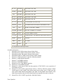
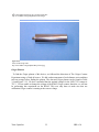
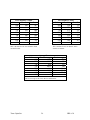
6.0.1 Assembly of the Geiger Muller Counter K2645
Label
Artnr
Qty
Description
BUZ1
SV3
C1
220J0C
1 ELCO PCB 220µF-16V
C13
.033/1K
1 33nF/1000V
C14
7MK47
1 MKH 0.047µF-250V
C2
SI100N0 1 SIBATIT 100nF-63V
C3
1MK1000 1 MKH 1µF-100V
1 SOUNDER VELLEMAN 3-30VDC 8mA/12V LEADS
C4
7M1
1 MKH 1nF-400V
C5...C12
7MK33
8 MKH 0.033µF-250V
D1...D4
1N4148
4 1N4148 (1N914)
D5...D14
1N4007 10 1N4007 DIODE 1A-1000V
BATTERY SNAP9V 1 BATTERY SNAP 9V "I" TYPE/LEADS 150mm
GM-TUBE GMTUBE 1 GEIGER-MULLER-TUBE
IC1
CD40106 1 CD40106BE HEX SCHMITT-TRIGGER
IC2
CD4093
J
DBL
Team CajunSat
1 CD4093BE 4 X 2 NAND SCHMITT-TRIGGER
1 JUMPER
49
FRR v3.0
R1...R3
RA10M0 3 RESISTOR 1/4W 10M
R10,R11 RA220K0 2 RESISTOR 1/4W 220K
R12
RA10K0 1 RESISTOR 1/4W 10K
R4...R7 RA100K0 4 RESISTOR 1/4W 100K
R8, R9
RA1M0
T1...T3
BC557B 3 BC557B SI-PNP UN 50V-0.2A
TRAFO1
LT44
14P
14P
2 RESISTOR 1/4W 1M
1 LT44 IMPEDANCETRANSFO 20KPRIM/1K SEC
2 14P DIL IC SOCKET 300MIL
BT20200 BT20200 2 BOLT M2 X 20mm CYL. HEAD
BUS1
BUS1
2 SPACER 10mm PLASTIC
FU-CLIP FU-CLIP 1 FUSEHOLDER CLIP MESSING BLANK FOR PCB
H2645
H2645
1 MANUAL
MR2
MR2
2 NUT 2mm
P2645
P2645
1 PCB
Table 3.5
This is the parts list for the Geiger counter.
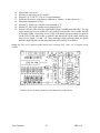
Assembly instructions:
1.
Mount R1 to R3, 10M resistors (brown, black, blue)
2.
Mount R4 to R7, 100K resistors (brown, black, yellow)
3.
Mount R8 and R9, 1M resistors (brown, black, green)
4.
Mount R10 and R11, 200K resistors (brown, black, orange)
5.
Mount C1, 220µF electrolytic capacitor. Mina the polarity!
6.
Mount C2, 100nF Sibatit capacitor
7.
Mount C3, 1µF MKM capacitor
8.
Mount C4, 1nF MKM capacitor
9.
MountC5 to C12, 33nF MKM capacitors
10. Mount C14, 47nF MKM capacitor
11. Mount C13, which may be either one big capacitor of 33nF/1000V or two capacitors of
47nF/400V in series.
12. Mount D1 to D4, smaller signal diodes 1N914 or 1N4146. Mind the polarity! Model
1n4148 may be color coded (wide yellow band, brown yellow, grey). In this case, the
wide yellow band should correspond to the mark on the printed circuit board. If the
diode shows number only, the black band should correspond to the mark on the pcb.
13. Mount D5 to D14, 1N4007 type diodes. Mind the Polarity!
Team CajunSat
50
FRR v3.0
14.
15.
16.
17.
18.
19.
20.
21.
Mount link J next to lC1
Mount a 14 pin socket for lC1 and lC2
Mount T1 to T3, BC557, 558, or 559 type transistors
Solder the black wire of the battery connector to “battery-“ to the red wire to “+”
Mount the transformer (LT44)
Mount lC1, 40106 type, with the recess pointing to T3
Mount 1C2, 4093 type with the recess pointing to lC1
Mount G.M. tube: take away the small ribbon (if any) winded around the tube. The clip
on the anode pin as to be pulled off (very gently!) from the tube. Never solder directly
to the tube! Solder a short strip of wire (2cm) to the anode clip and connect it to point A
on the PCB. Fit the tube socket on point K, and then break off the small tooth at one
end of it (see figure 3.11 and 3.12). After soldering is done (and only then) you gently
push the anode clip back on the tube and fit the tube carefully in its holder.
NOTE: This came from a translated product manual from Velleman®, INC. There were no English versions
available.
Figure 3.16
Schematic drawing for the Geiger Muller Counter K2645 from product manual.
Team CajunSat
51
FRR v3.0
Figure 3.17
Schematic drawing for the Geiger Muller Counter K2645 from product manual.
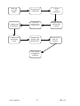
The following is the method that we will use in constructing our payload; however, while we
are doing this we will also be adding everything to the PDR, CDR, and FRR. This is not stated in
the procedures, but it will be done.
1.
Build and test a cold chamber to house our payload, vacuum chamber, and dry ice with
the ability to maintain a temperature of about -60°C.
2.
Do a vacuum test of all the components of our payload to see if it out gases and can
function in a low pressure environment.
3.
Cold test all of the components individually to find the minimum operating range of the
components and the max lower temperature possible for it to still function.
4.
Design and test our box for both structural and thermal support.
5.
Complete the BalloonSAT and Geiger counter.
6.
Complete and Test the software to run the BalloonSAT and Geiger counter.
7.
Complete and test the heating circuit.
8.
Integrate the heating circuit to the BalloonSAT.
9.
Find the Dead time for the payload.
10. Complete full systems test of the payload to make sure we are getting accurate results
and can survive assembled together with all the items of our payload.
Team CajunSat
52
FRR v3.0
Build and
test cold
camber
Vacuum test all
components
Cold test
each
component
Complete and
test Software
Complete the
BalloonSAT and
Geiger counter
Design and test
box used for
payload
Complete and
test heating
circuit
Integrate the
heaters with
BalloonSAT
Find the Dead
time for
payload
Full systems
test under all
conditions
Team CajunSat
53
FRR v3.0
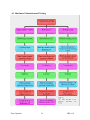
6.1 Hardware Fabrication and Testing
Team CajunSat
54
FRR v3.0
6.1.2Dead
DeadTime
time
3.1.7
Geiger Counter
One of the things that must be done is calculating the dead time of each detector
because without this information we will get inaccurate data. We will find the dead time
by performing an experiment created by the Syracuse University Physics department and
can be found at the following address:
http://www.phy.syr.edu/courses/PHY344.05Spring/Geiger_Mueller_counter.pdf
Team CajunSat
55
FRR v3.0
Team CajunSat
56
FRR v3.0
6.1.3 Flux Calculations
After finding the area of the Geiger counters, dead time, and voltage plateau we are finally able
to find and compare the flux, rate of flow per unit area, of the cosmic rays. We will do this by
using the following flux formula:
The previous formula is the general formula for flux that does not include the dead time of the
detector. The following formula includes the dead time of the detector and will give us an
accurate flux measurement.
Because our area and time will be constant, we can rewrite the flux formula in the following
way:
This is for the K2645 Geiger counter while the next formula is for the LND 7232 Geiger
Counter.
To calculate the flux of each detector we will place a Strontium-90 (beta source) 9 cm away
from the detector. We will then record the counts once per minute and then calculate the flux
with our measured data. After completing this experiment we calculated the fluxes of each
Geiger counter to be the following:
Team CajunSat
57
FRR v3.0
K 2645 Geiger Counter
44 minute run
Minutes Counts
1
28
2
38
3
39
4
24
5
43
6
36
7
46
8
33
9
50
10
36
11
46
12
22
13
39
14
31
Average
Minutes
15
16
17
18
19
20
21
22
23
24
25
26
27
28
29
Counts
30
34
36
37
34
31
27
39
45
29
26
43
42
31
32
Minutes
30
31
32
33
34
35
36
37
38
39
40
41
42
43
44
Counts
37
35
26
34
44
37
31
31
33
41
30
31
25
33
18
34 counts
Table 3.7
This is the Data from one of our runs with the Geiger counter.
Team CajunSat
58
FRR v3.0
LND 7323 Geiger counter data
Time
60.05
59.87
59.7
60.06
59.9
59.76
60.02
59.88
59.95
59.78
59.95
60.17
60.04
60.15
59.81
60.13
60.3
60.06
60.17
60
59.82
60.3
59.97
counts
143
110
139
128
118
123
129
129
132
128
135
140
127
134
127
143
121
109
126
120
143
122
109
flux
22.24089852
17.15982007
21.74551872
19.90462246
18.39858772
19.22311771
20.07349629
20.12042831
20.56430548
19.99785254
21.03167605
21.73088067
19.75569625
20.80647311
19.83166699
22.2113081
18.74119852
16.95003006
19.5577926
18.67924414
22.32641184
18.89608445
16.97546783
flux w/
dead time
22.24784146
17.16519297
21.75234684
19.91083506
18.4043456
19.22914773
20.07976577
20.12672714
20.57073575
20.00412348
21.03825247
21.73765087
19.76186442
20.81295747
19.8378827
22.21823258
18.7470247
16.95532048
19.56388578
18.6850801
22.33340828
18.90195878
16.98077413
Average counts
Time
59.88
59.82
60.13
59.82
59.96
60.05
60.22
60.18
61.03
59.77
60.11
60.12
59.74
60.25
59.77
60.09
59.56
59.82
60.18
62.2
counts
143
121
129
114
114
118
133
114
121
133
112
119
119
129
135
113
120
115
142
143
flux
22.30404068
18.89157925
20.03677444
17.79867797
17.75712001
18.35262955
20.62719587
17.69220532
18.51702885
20.78249515
17.40205743
18.48661055
18.60420198
19.99686717
21.09501388
17.56327665
18.81723721
17.95480672
22.03765926
21.47212148
flux w/
dead time
22.31102311
18.89749932
20.043021
17.80425555
17.76267158
18.35835869
20.63361688
17.69771636
18.52271646
20.78901323
17.4074844
18.4923748
18.6100398
20.00308887
21.10162997
17.56875573
18.82315974
17.96043323
22.04452389
21.47859267
128
Comparing the flux we can conclude that the K2645 is getting the same amount of radiation
per square centimeter. Therefore, we can now conclude that our K2645 Geiger counter is ready
to be flown.
Team CajunSat
2
FRR v3.0
6.1.4 Calibration of Geiger counter at sea level
To make sure that our flux is accurate, we will run our Geiger counter at sea level for a few
hours and then compare it to the flux at sea level, which happens to be the following:
Once our flux at sea level is correct, we can expect our flight to resemble Figure 3.19. This is a
theoretical curve for the flux per altitude. We notice that we should have an exponential growth
until we reach approximately 15 km then we expect it decay exponentially after this point. The
reason for this has to do with the interaction length of the particles and we be explained in the
next section.
6.1.5 Calibration of Geiger Counter
The Geiger counter we will be using to calibrate the K2645 Geiger counter is a Spectech ST350 counter made by Spectrum Techniques with a LND 7232 Geiger Muller tube made by LND,
Inc. The specifications on each of them is as follows:
Team CajunSat
50
FRR v3.0
Spectech ST-350 counter
Table 3.1
This is a copy of the Specifications of the Spectech ST-350 system from the user manual.
http://www.spectrumtechniques.com/manuals/ST350manual.pdf
Team CajunSat
51
FRR v3.0
Figure 3.10
This is a picture of our equipment together.
LND 7232 Geiger Muller Tube
General Specifications
Gas Filling
Ne +Halogen
Cathode Material
446 Stainless Steel
Maximum Length (inch/mm)
4.85 / 123.1
Effective Length (inch/mm)
2.6 / 66.04
Maximum Diameter (inch/mm)
1.38 / 34.9
Effective Diameter (inch/mm)
1.13 / 28.6
Connector
BNC
0
Operating Temperature Range C
-55 to +75
Table 3.2
This is the general specifications of the Geiger Muller tube.
http://www.lndinc.com/gm/alpha/7232.htm
Team CajunSat
52
FRR v3.0
Window Specifications
2
Areal Density (mg/cm )
2.0
Effective Diameter (inch/mm)
1.13 / 28.6
Material
Mica
Table 3.3
This is the window specifications of the Geiger tube.
http://www.lndinc.com/gm/alpha/7232.htm
Electrical Specifications
Recommended Anode Resistor (meg ohm)
1
Maximum Starting Voltage (volts)
800
Recommended Operating Voltage (volts)
900
Operating Voltage Range (volts)
850-1000
Maximum Plateau Slope (%/100 volts)
10
Minimum Dead Time (micro sec)
150
60
Gamma Sensitivity Co (cps/mR/hr)
40
Maximum Background Shielded 50mmPb + 3mmAl (cpm)
50
Tube Capacitance (pf)
3
Weight (grams)
155
Table 3.3
This is the electrical specifications of the Geiger tube
http://www.lndinc.com/gm/alpha/7232.htm
Team CajunSat
53
FRR v3.0
Figure 6.10
Circuit drawing for the Geiger tube.
http://www.lndinc.com/gm/alpha/7232.htm
Team CajunSat
54
FRR v3.0
Figure 6.11
This is the gamma sensitivity curve for the Geiger tube.
http://www.lndinc.com/gm/alpha/draw/sen7232.gif
Figure 6.12
Picture of the Geiger tube.
http://www.lndinc.com/gm/alpha/draw/pic7232.jpg
Geiger Plateau
To find the Geiger plateau of this device, we followed the directions of The Geiger Counter
Experiment using a Cobalt-60 source. We did each measurement of each distance twice and then
took an average before finding the plateau. The data and Geiger plateau can be found in Table
3.4 and Figure 3.12. We have concluded that the optimal voltage for the LND 7323 counter is
725 V. We are unable to change the voltage of the K2645 Geiger counter; therefore, we will not
be performing this experiment on the K2645. This was only done to make sure that our
calibration Geiger counter is running at the correct voltage.
Team CajunSat
55
FRR v3.0
Close Distance Counts
Volts
Run 1
Run 2
800
896
775
896
750
916
725
866
700
840
675
859
650
650
625
0
Far Distance Counts
Volts
Run 1
Run 2
800
328
336
775
271
271
750
273
231
725
287
213
700
256
235
675
256
225
650
186
215
625
0
0
987
891
864
873
848
766
732
0
Table 3.4 A
This is the data for our close distance which
was the first slot.
Volts
800
775
750
725
700
675
650
625
Table 3.4 B
This is the data for our far distance which
was the second slot.
Average Counts
Close Average
941.5
893.5
890
869.5
844
812.5
691
0
Far Average
332
271
252
250
245.5
240.5
200.5
0
Table 3.4 C
This is an average of all of our data for each distance.
Team CajunSat
56
FRR v3.0
Figure 3.12
This is our experimental Geiger plateau. We can see that the optimal voltage is 725 V.
Once we figure out the Geiger plateau for the LND 7232 we will use it to make sure that it is
operating at the correct operating voltage. After this, we will take a Strontium-90 source and
place it an inch away from the detector. We will then take measurements in one minute intervals
and calculate the flux. After we do this, we will compare the results of each Geiger counter.
Team CajunSat
57
FRR v3.0
Figure 6.1
Theoretical calculated flux of cosmic rays with respect to altitude.
http://hyperphysics.phy-astr.gsu.edu/hbase/astro/cosmic.html
Vacuum testing procedures
Seal the vacuum chamber without anything inside and then measure the amount of time that it
took for the vacuum to go all the way down. Then place the object you want to vacuum test
inside and measure that time. If it takes longer, then there is some outguessing occurring. Also,
observing the object inside and looking for fumes is something else that we try to do. The final
test is to take a close look at the object after it is finished with the vacuum test to see if there are
any significant changes such as becoming brittle.
Cold testing procedures
The first thing we do is get between 10-20 lbs of dry ice at a U-Haul place near campus. Then
we place the object in our cold chamber see Figure 11.18 B. Next, we put the dry ice around the
object, but not touching the object. We then place temperature probes in the cold chamber to get
Team CajunSat
58
FRR v3.0
the temperature of the objects environment and place either a HOBO or temperature probe inside
with our object. Finally, we let in stay in that environment and observe the results.
Minimum operating temperature procedures
To find the minimum operating temperature we do a cold test on the environment and see how
the object performs as the temperature goes down. When the object can no longer operate as it is
designed to, we record the minimum operating temperature and try to keep it within its operating
limits.
Geiger counter test
To test the Geiger counter, we will place a Cobalt-60 source at a certain distance and let it
record the counts per minute. We will also take another Geiger counter and do the same thing to
it. After both test are complete, we will compare the results of the Geiger counters.
Integration
After the heaters and Geiger counters are constructed and working properly, we will connect
them to the BalloonSAT. When they are connected, we will run tests to make sure that they
function with the BalloonSAT and can store the data on the BalloonSAT. The heaters must be
able to be turned off and on as the temperature drops to below 0°C.
6.3 Software Implementation and Verification
The Basic stamp will run the following program. This program is designed to get the counts,
temperature, and turn on the heater if the temperature gets too cold inside.
' {$STAMP BS2}
' {$PBASIC 2.5}
gmcount VAR Word
gmin PIN 5
ee1da PIN 8
ee1cs PIN ee1da+1
ee2da PIN 0
ee2cs PIN ee2da+1
tempda PIN 13
tempcl PIN 14
tempcs PIN 15
ch1sel CON %1110
ch2sel CON %1101
temp
VAR Byte
nexttemp VAR Word
Team CajunSat
'set geiger input pin
'labels temp eeprom
'chip enable pin
'labels temp eeprom
'chip enable pin
'adc8031 data pin
'adc0831 clock pin
'adc0831 chip enable pin
'adc0831 channel 1 constant
'adc0831 channel 2 constant
'used for adc0831 data
'used for temp eeprom address
59
FRR v3.0
addrblock VAR Word
heater PIN 7
addrl VAR Word
addrh VAR Word
beeper PIN 4
'used for temp eeprom address
'used to turn on and off heater
'lsb byte for gm count storage
'msb byte for gm count storage
'buzzer pin
main:
LOW heater
' make sure heater is off
FREQOUT 4,1000,300
' produce tone to demostrate proper
operation
READ 3,addrblock
' set start of mem address
READ 2,nexttemp
'
"
READ 1,addrh
'
"
READ 0,addrl
'
"
DO
LOW tempcs
SHIFTOUT tempda,tempcl,LSBPOST,[ch1sel]
' initiate adc0834
COUNT gmin, 3484, gmcount
' read 1 sec of G-M collisions
'DEBUG DEC gmcount.LOWBYTE," ", DEC addrh, DEC addrl, CR
I2COUT ee1da, $A0, addrh\addrl, [gmcount.HIGHBYTE] ' store counts msb*8
addrl = addrl + 1
PAUSE 4
I2COUT ee1da, $A0, addrh\addrl, [gmcount.LOWBYTE] ' store counts lsb*8
addrl = addrl + 1
WRITE 0,addrl
' update mem location
SHIFTIN tempda,tempcl, MSBPOST, [temp\9]
' read inside temp
I2COUT ee2da, $A0, addrblock\nexttemp, [temp] ' store inside temp
nexttemp=nexttemp+1
'DEBUG DEC temp,CR
' this line for outputting temps
' while running
HIGH tempcs
LOW tempcs
' initiate adc0834
SHIFTOUT tempda,tempcl,LSBPOST,[ch2sel]
PAUSE 10
SHIFTIN tempda,tempcl, MSBPOST, [temp\9]
' read outside temp
I2COUT ee2da, $A0, addrblock\nexttemp, [temp] ' store outside temp
nexttemp=nexttemp+1
'DEBUG DEC temp, CR
' this line for outputting temps
WRITE 2,nexttemp
' while running
Team CajunSat
60
FRR v3.0
HIGH tempcs
IF addrl >= 255 THEN
' this section is for updating msb
'DEBUG DEC addrl, " ",DEC addrh, CR
' block info for count storage
addrl = 0
addrh = addrh + 1
WRITE 1,addrh
FREQOUT 4,100,300
' test beep for varification of operation
ENDIF
' occurs about every 4 minutes
IF nexttemp >=256 THEN
addrblock = addrblock +1
nexttemp = 0
WRITE 3,addrblock
ENDIF
' updates msb for temp storage
IF addrh > 7 THEN
HIGH heater
ENDIF
LOOP
' after 1/2 an hour...
' turn on heater
The following program is designed to convert the bit data from the EEPROM to temperature in
ºC. It will be used for us to make sure that our payload stayed within the correct operating
temperature.
' {$STAMP BS2p}
' {$PBASIC 2.5}
' This program is made to read temp data off eeprom 2
SDA
SCL
addrlow
addrhigh
value
result
PIN
PIN
0
' I2C SDA pin
SDA + 1
VAR Word
VAR Word
VAR Byte
VAR Byte
Team CajunSat
' internal address
' internal address
' value to write
' array for returned value
61
FRR v3.0
Read_From_EEPROM:
DEBUG CR, "Reading...", CR
FOR addrhigh = 0 TO 255
FOR addrlow = 0 TO 255
I2CIN SDA, $A1 , addrhigh\addrlow, [tempout]
addrlow=addrlow+1
PAUSE 10
I2CIN sda, $A1, addrhigh\addrlow, [tempin]
addrlow=addrlow+1
PAUSE 10
'DEBUG DEC addrlow,CR
DEBUG DEC tempin," inside",CR
DEBUG DEC tempout," outside",CR
NEXT
NEXT
PAUSE 100
DEBUG CR, "All locations read"
END
Team CajunSat
62
FRR v3.0
This program is designed to clear the data off the EEPROMS.
' This program clears out the eeproms on the balloon project board, one at a time.
' Then checks for zero's in all locations of gm eeprom
'
' {$STAMP BS2p}
' {$PBASIC 2.5}
SDgm
SCLgm
sdtemp
scltemp
addrlow
addrhigh
value
result
PIN 8
' "8" clears G-M,
PIN SDgm + 1
PIN 0
' "0" clears temps
PIN sdtemp + 1
VAR Word
VAR Word
VAR Byte
VAR Byte
' internal address lsb
' internal address msb
' value to write
' array for returned value
Write_To_gm_EEPROM:
value = %00000000
' binary zero
DEBUG "Writing to eeprom 1...", CR
PAUSE 20
FOR addrhigh = 0 TO 255
FOR addrlow = 0 TO 255
' loop through all addresses
I2COUT SDgm, $A0, addrhigh\addrlow, [value]
' load zero
PAUSE 10
'DEBUG "Addr: ", DEC3 addrhigh, " ",DEC addrlow,
' " Value: ", DEC3 value, CR
NEXT
NEXT
PAUSE 20
Write_To_temp_EEPROM:
DEBUG "Writing to eeprom 2...", CR
PAUSE 20
FOR addrhigh = 0 TO 255
FOR addrlow = 0 TO 255
' loop through all addresses
I2COUT sdtemp, $A0, addrhigh\addrlow, [value]
' load zero
PAUSE 10
'DEBUG "Addr: ", DEC3 addrhigh, " ",DEC addrlow,
' " Value: ", DEC3 value, CR
NEXT
NEXT
Read_From_EEPROM:
DEBUG CR, "Reading...", CR
Team CajunSat
63
FRR v3.0
FOR addrhigh = 0 TO 255
FOR addrlow = 0 TO 255
I2CIN SDgm, $A1 , addrhigh\addrlow, [result]
'DEBUG " ", DEC3 result
IF result > 0 THEN
DEBUG "error at loc: ",DEC addrhigh," ",DEC addrlow,CR
ENDIF
PAUSE 10
NEXT
NEXT
PAUSE 100
DEBUG CR, "All locations cleared",CR
END
Team CajunSat
64
FRR v3.0
This program will allow us to get the counts from the EEPROM and display then counts in
counts per minute. We will then use EXCEL to calculate the flux.
' I2C.BSP
' This program outputs the data of the gm eeprom
' and displays the information by minute.
'
' {$STAMP BS2p}
' {$PBASIC 2.5}
SDA
SCL
PIN
PIN
8
' I2C SDA pin
SDA + 1
addrlow
VAR Word
addrhigh
VAR Word
block
VAR Nib
value
VAR Byte
result
VAR Byte
mincount
VAR Word
MINtotal
VAR Word
minnum
VAR Word
' internal address
' internal address
' block address in 24LC16
' value to write
' array for returned value
' number of mem locations read
' number of counts
' number of minute being totalled
Read_From_EEPROM:
minnum=0
mincount=0
mintotal=0
DEBUG CR, "Reading...", CR
FOR addrhigh = 0 TO 255
FOR addrlow = 0 TO 255
mincount=mincount+1
I2CIN SDA, $A1 , addrhigh\addrlow, [result]
mintotal=mintotal + result
IF mincount=120 THEN
mincount=0
minnum=minnum + 1
DEBUG DEC mintotal, " counts in minute ",DEC MINnum, CR
mintotal = 0
ENDIF
NEXT
NEXT
PAUSE 100
DEBUG CR, "All locations read"
END
Team CajunSat
65
FRR v3.0
This program erases all the data stored on the EEPROM.
' {$STAMP BS2p}
' {$PBASIC 2.5}
' This program sets the eeprom memory locations to start at zero
WRITE 0,0
WRITE 1,0
WRITE 2,0
WRITE 3,0
END
We will calculate the dead time of our software once the flight is over. The procedures for this
are discussed in the dead time section.
Team CajunSat
66
FRR v3.0
6.4 Flight Certification Testing
-
Conditions
o Temperatures ≈ -60 oC.
o Low pressures ≈ 1% atmosphere.
o Rotation around the z-axis
o Possible turbulence
o Impact ≈ 6 m/s
-
Compensation and Testing
o In order to ensure a successful flight, we will test all equipment multiple times.
This includes doing vacuum, cold, and impact testing both individually and all
three at the same time. We will do what needs to be done to make sure all of our
equipment can survive its environment.
o All of our testing procedures produce an environment that is a little rougher than
what is expected. This ensures that our payload will survive and function as it is
designed.
7.0 Mission Operations
The payload will be launched and tracked from the ground by a separate GPS unit. It will be
recovered upon landing. The following operations will be performed pre-flight, and post flight:
Pre Flight Operations:
- Full system test of hardware
- New batteries are to be placed in payload for maximum voltage
- Check all structures to make sure they are properly fastened down
- Make sure lids are properly sealed
- Properly attach payload to balloon
Recovery and data extraction
- Take pictures
- Record observations
- Examine for mechanical damages
- Examine the payload and see if there are any damages in the integrity of the system
- Disassemble the payload and extract the BASIC Stamp.
- Download the data from EEPROM through the serial cable connection on the
BalloonSAT board and process it on a computer
- Take a ground test of Geiger counter again to make sure it is functioning properly.
Data Analysis
- Check if data has been collected for the entire duration of the flight
- Plot the flux with respect to altitude (using the GPS data from a tracking unit)
- Check if the plotted data agrees with the expected theoretical curve (Figure 3.18)
Team CajunSat
67
FRR v3.0
7.1 Launch Requirements
Final testing
- check if the separate parts of the payload are operable and are powered on (BASIC
Stamp, Geiger counter, heating unit)
- check if the parts interact as designed and work as a whole
- check power sources for output voltages and currents and replace by a new spare if
needed
- check control points for proper voltages on them
- check the integrity of the system (make sure everything holds firm inside the cube
- verify GPS synchronization
- proper sealing of payload and attachment to balloon vehicle
All test should give a positive result and all malfunctioning revealed should be taken into
consideration and fixed in field
A full cycle test run should be done in field. This will simulate the data acquisition during the
flight. This also will allow us to make sure that everything is still functional after the
transportation
7.2 Flight Requirements and Operations
Flight Requirements
- payload must reach a height of at least 15 km
- heating devices must maintain the payloads temperature to a minimum value of -20 ºC
- proper synchronization of all devices inside, and outside of the payload
Post flight Requirements
- GPS time, latitude, longitude, and altitude to properly analyze our data
- Proper functioning of all interior devices (Geiger Counter, BalloonSAT) in order to
collect needed graphs and data
7.3 Data Acquisition and Analysis Plan
The Velleman K2645 Geiger-Muller Counter will be interfaced to the BASIC stamp allowing
all data from the Geiger counter to be stored into the EEPROM of the BASIC Stamp as standard
units of counts per minutes. Post flight the data will be collected via computer and a pre-written,
pre-tested program will convert the units of counts per minute to flux, refer to section 3.1 for
details about these conversions. Once we have collected all necessary data including GPS time,
latitude, longitude, and altitude from the tracking team. Graphs will be acquired in order for
comparison to expected results. Error will be calculated between acquired results and expected
results. This error will be included in the final data analysis.
Team CajunSat
68
FRR v3.0
8.0 Project Management
We will meet on Thursdays from 5:00 pm till 8:00 pm and on Fridays from 2:30 pm till 7:00
pm for group work. These sessions are to discuss completed sections and decide on future
workflow. We will discuss any problems encountered and methods chosen to correct them. Any
additional group work periods are scheduled as needed. All individuals will be expected to
complete their sections according to schedule and work independently on their own time if
necessary. Any changes to payload or schedule will be voted on during group sessions. This is
needed so we will be able to determine potential budget or deadline issues. The team leader will
be responsible for overall project flow and will actively monitor the budget and progress. Every
team member is responsible for keeping accurate records on their respective sections, and team
record keeper will centralize the records as needed. Any parts needed will be ordered by the
graduate assistants or by project oversight.
Team CajunSat
69
FRR v3.0
8.1 Organization and Responsibilities
PROJECT OVERSIGHT
Dr. William A. Hollerman
Graduate Assistant
Graduate Assistant
Noah Bergeron
Mikhail Yevdokimov
Team Leader
Robert Moore
Payload Design
Jasmine Bulliard
Donald Crouch
Payload Testing
Robert Moore
Payload Management
Ross Fontenot
Environmental
Testing
Mechanical Design
Documentation
Payload Electrical
Testing
Thermal
Parts Acquisition
Electronics Design
Accounting
Software Design
Overall System
Design
Contact Information:
Dr. William A. Hollerman:
[email protected]
Noah Bergeron:
[email protected]
Mikhail Yevdokimov:
[email protected]
Robert Moore:
[email protected]
Ross Fontenot:
[email protected]
Jasmine Bulliard:
[email protected]
Donald Crouch:
[email protected]
Team CajunSat
70
FRR v3.0
8.2 Configuration Management Plan
Any changes to payload design are implemented according to following procedures:
Design Change Plan:
1.
2.
3.
4.
5.
Change request posed during team meeting.
All members of team votes on change.
Budget monitor will assure change fits in budget and advise team leader
Team leader will give final approval.
Record keeper will document relevant PDR/CDR sections.
8.3 Interface Control
There will be four main interfaces. They include:
1.
2.
3.
4.
Electrical interface
Mechanical interface
Software interface
General interface
(Section 4.3)
(Section 4.5)
(Section 8.3)
(Section 8.3)
Note: any changes to the interface design will follow the same procedures listed in Section 8.2.
8.3.1 Electric Interface
Electric interface is the electronic connection between the subsystems. The specific interfaces
are:
1.
2.
3.
4.
Switch to batteries
Batteries to BalloonSAT
Interface board to Geiger counter
BalloonSAT to heaters
8.3.2 Mechanical Interface
This is the structural connection between each system. The specific interfaces include the
following:
1.
2.
3.
4.
5.
6.
Box to Balloon *
BalloonSAT to box
Heaters to box
Geiger Counter to box
Batteries to box
Switch to box
*This will following the guidelines in LaACES lecture Payload Construction
Considerations and Techniques.
Team CajunSat
71
FRR v3.0
8.3.3 Software Interfaces
The software programming needed to central subsystems, store measurements, and retrieve
data after flight is known as software interfaces. It will include the following:
1.
2.
3.
4.
Program to provide timing for data collection
Program to save raw data
Program to convert raw data to formatted data
Program to retrieve data
8.3.4 General Interfaces
These are the interfaces between the various levels of entire project. The specific interfaces are
in the following list:
1. Interface between CajunSat team members
• Interpersonal communication will occur at CajunSat team meetings to provide
weekly updates on progress. Email, telephone and face-to-face communication
will be used to convey important messages between team members.
2. Interface with Stakeholders
• Interfacing between CajunSat team members and Stakeholders will be in the form
of written PDR, CDR, and FRR. Formal presentations will also be prepared and
will allow direct interaction.
3. Interface with Project Management
• Interfacing between CajunSat team members and project management will occur
via interpersonal communication either during scheduled team meetings and
office meetings.
9.0 Master Schedule
The following two sections are the overall work flow plan. Any changes to these will follow
procedures listed in section 8.2. The tasks listed in the WBS were assigned to the various team
members according to their strengths. Any team member who is not assigned a task for a specific
date will assist others with their tasks. All dates listed are on our scheduled work days, Thursday
and Friday. If for some reason we can not finish any particular task on the scheduled date it will
be accomplished during the rest of the week.
There are many times during Monday through Wednesday where we have free time to meet.
This will aid in finishing all tasks in the manner and timing set forth in the Gant chart. Any
additional time needed will push the final few tasks into early May, which has only scheduled
dates for the preparation for FRR and flight operations.
Team CajunSat
72
FRR v3.0
9.1 Work Breakdown Structure (WBS)
Section 9.1 Work Breakdown Structure (WBS) and Staffing Plan
I. Lithium battery load check:
Ross
II. Design heating circuit:
1. Build heating circuit:
2. Test heating circuit:
Jasmine, Donald
Ross
Ross
III. Build Geiger counter kit:
1. Geiger counter rate check:
2. Geiger counter accuracy check:
3. Geiger counter environmental check:
Jasmine, Donald
Ross
Ross
Ross
IV. Design interface board:
1. Build interface board:
Jasmine, Donald
Jasmine, Donald
V. Build a system mock-up for testing:
1. Interface communication test:
2. Interface baseline check:
Robert
Jasmine, Robert, Ross, Donald
Jasmine, Robert, Ross, Donald
VI. Prepare CDR documents:
Mikhail
VII. Design structural layout:
Jasmine, Donald
VIII. Build a system mock-up for testing:
1. System mock-up shock test:
2. System mockup environmental check without heater:
3. System mockup environmental check with heater:
Robert
Jasmine, Robert, Ross, Donald
Jasmine, Robert, Ross, Donald
Jasmine, Robert, Ross, Donald
IX. Build final payload:
1. Final system checks:
Robert
Jasmine, Robert, Ross, Donald
X. Prepare FRR documents:
Jasmine, Robert, Ross, Donald
Team CajunSat
73
FRR v3.0
9.2 Staffing Plan
Team CajunSat
74
FRR v3.0
9.3 Timeline and Milestones
Team CajunSat
75
FRR v3.0
10.0 Master Budget
Item
Figure 10.1
Table of the costs
Estimated
Cost
Description
-
Batteries
$60.00
Gamma
Scout
Donated
Velleman
K2645
GeigerMuller
Counter Kit
$150.00
Additional
Supplies for
Geiger
Counter
Pricing Comments
Lithium Batteries
producing 9V
Batteries for actual flight,
and for testing
-
No wait time
purchased at local
retail store
-
Used as a back up for the
Velleman K2645 GeigerMuller Counter Kit
-
express shipment
approximately 2-5
day wait period
-
Used for detection of beta
and gamma radiation in
final payload
-
express shipment
approximately 2-5
day wait period
-
Supplies for interfacing the
BASIC STAMP to the
Velleman K2645 GeigerMuller Counter in the
account it becomes our
primary user
-
$20.00
Heating
Lead Time
$10.00
-
No wait time
purchased at local
retail store
-
No wait time
purchased at local
retail store
Ceramic resistors used for
heating payload
-
approximately
$11.00 per 9V
battery
-
donated for UL
of Lafayette
LaACES use no
cost to budget
-
detailed
information is
listed below (**)
-
approximately
$1 - $2 per item
used to construct
this portion of
the payload
-
Ceramic resistors
99 cents per
resistor at Radio
Shack
Most costly
items were board
to build box
which is around
$20 for enough
to build final
box, and have
spare for testing
needs
Dry ice was the
most costly item.
We regularly
purchased dry
ice for our
testing
Final
Building
Supplies
Testing
Supplies
$50.00
$75.00
-
Foam board for building
payload, epoxy, wires, etc.
-
Foam board for designing
cold chamber, dry ice, etc
-
No wait time
purchased at local
retail store
-
No wait time
purchased at local
retail store
-
Total
Estimated
Cost
$365.00
Table 10.1
Budget Table
** Four suppliers for the V-K2645 Geiger-Muller Counter kit (part# N32VKK2645)
were priced to be the most cost efficient with the budget. The result of our
research was as follows:
Team CajunSat
76
FRR v3.0
- PogeeKits Electronic Kits and Tools
http://www.apogeekits.com/geiger_counter.htm
- Gibson Tech Ed, Inc
http://www.gibsonteched.com/vk2645.html
- Carl’s Electronics Inc.
http://www.electronickits.com/kit/complete/meas/vek2645.htm
- Electronix Express
http://www.elexp.com/kit_2645.htm
$148.50
$143.99
$179.95
$139.95
** We determine to go with PogeeKits Electronic Kits and Tools. The two suppliers with
lower prices were sold out of the V-K2645, which would have resulted in a longer
wait period that our project could not afford.
- It is possible more money will need to be allocated to purchasing additional
supplies (batteries, heating, etc). According to the below Fig 10.2, we have 27% of our
budget left to cover additional expenses we may encounter.
10.1 Expenditure Plan
UL Lafayette LaACES Budget
$60.00
12%
$135.00
27%
Batteries
Velleman Geiger counter
$150.00
30%
$75.00
15%
Additional supplies for
Geiger counter
Heating
Building supplies
$50.00
10%
$10.00
2%
$20.00
4%
Testing supplies
Left over budget
Figure 10.2.
This is a pie graph that shows the distribution of funds.
At this point in time we have purchased batteries, the Velleman K2645 Geiger-Muller Counter
Kit, testing supplies, and some building supplies. The lithium batteries will have two purposes in
our LaACES program. First, we will use at least two batteries for testing voltage drop (cold
Team CajunSat
77
FRR v3.0
testing, vacuum testing, and cold vacuum testing). The second use for the batteries will be in
powering the electrical components within our payload. We will use two 9V lithium batteries to
power the load. Referring to figure 10.2, battery cost was 12% of our budget. The Velleman
K2645 Geiger-Muller Counter was purchased for approximately $150.00. Since it was one of our
most costly items, 30% of our budget (Figure 10.2), we researched multiple suppliers in order to
be the most cost efficient. These details are located in the above section 10.0. Testing supplies
have been purchased multiple times during programs timeframe. The biggest expense that we
have encountered with testing supplies is dry ice, which is $1.00/pound. We used dry ice on a
regular basis for our testing procedures of all of our components that are to go in the final
payload. According to Figure 10.2, testing supplies will take approximately 15% of our budget.
We have purchased some building supplies, although more will be purchased when the time
comes to build the final payload. Building supplies mostly includes foam board, aluminum tape,
glue (epoxy), and other small items, these supplies take up approximately 10% of our budget
(Figure 10.2). The only other expenditure that we have not yet purchased is the heating coils,
used for marinating our payloads temperature around a minimum of -20 ºC. Heating elements
will only take up 2% of our budget according to Figure 10.2. We have 27% of our budget left
over after accounting for all expected expenditures. Therefore we will have more then enough
left over budget to account for additional supplies we may need.
10.2 Material Acquisition Plan
Item
Acquisition
Batteries
Purchased
Vacuum chamber
Existing Supplies
Dry Ice
Purchased
Cold Chamber
Existing Supplies
Heating Elements
Insulation
Purchased
Existing Supplies
Existing Supplies/
Purchased
Existing Supplies/
Purchased
Existing Supplies/
Purchased
Electrical Components
Building Supplies
Testing Supplies
Order
Date
Need Date
Needed on multiple accounts
throughout entire project
Needed on a regular basis for
testing
Purchased as needed for project
Built on 2/10/05, used for testing
on a regular basis
3/24/05
3/24/05
3/24/05
2/24/05
Purchased as needed for the
project
Geiger-Muller Counter
Purchased
3/8/05
3/24/05
Gamma Scout
Donated
3/3/05
3/24/05
Figure 10.3
Purchasing record.
Team CajunSat
78
FRR v3.0
11.0 Risk Management and Contingency
In order for us to have a successful flight, we must do lots of testing. This ranges from cold
testing, vacuum testing, impact testing, and equipment testing. The following section explains
and gives results of the different testing we did.
11.1 Stress testing
The first test we did was a stress test of the box rolling it down a flight a stairs. One thing that
was noticed is that our only problem will be us securing our payload to the box. We solved this
by installing slits in the boxes. The different slits will provide the stabilization at impact and will
be able to survive just about any kind of impact except maybe a parachute failure. We did not
roll our slit design down the stairs, but instead threw it our of a second story window. See figure
11.2. Surprisingly, there was very little damage to the outside of the box and only a broken piece
of balsa wood and dented slit. This is not a problem because the batteries are on the bottom and
only would break the heaters.
Figure 11.1.A
This is at the bottom of where we roll our foam box
down the stairs and then observe what happens.
Team CajunSat
79
Figure 11.1.B
This is at the top of where we roll our foam box down
the stairs and then observe what happens.
FRR v3.0
Figure 11.1.C
Pretesting of box
Figure 11.1.D
Outside of box after we threw it down the
stairs
Figure 11.1.E
What happened on the inside. The glue did not
hold well and we actually ripped a battery
bottom off on upper left picture.
Figure 11.2 A
Picture from the second story window.
Team CajunSat
80
FRR v3.0
Figure 11.2 B
Picture of the second story window where we threw out the box.
Figure 11.2 C
Picture of the landing
Team CajunSat
81
FRR v3.0
Figure 11.2 D
Close up of our box after the landing
Figure 11.2 E
Close up of our box after the landing
Team CajunSat
82
FRR v3.0
Figure 11.2 F
This is a picture of the top layer of our payload. This is what will house the Geiger counter.
Figure 11.2 G
This is a picture of the top layer of our payload. This is what will house the BalloonSAT.
Team CajunSat
83
FRR v3.0
Figure 11.2 H
This is what happened to our battery section.
Figure 11.2 I
This is what happened to our battery section
Team CajunSat
84
FRR v3.0
Figure 11.2 J
This is what happened to our battery section
Figure 11.2 K
This is what happened to our battery section
Team CajunSat
85
FRR v3.0
Figure 11.2 L
This is a close up of our inner box. The holes are where we slide in a section of the Balsa wood
or section.
Figure 11.2 M
This is a close up of our inner box. The holes are where we slide in a section of the Balsa wood
or section.
Team CajunSat
86
FRR v3.0
11.2 Cold testing
Cl-6450 Scientific Workshop
The instrument we use for our experiments is Cl-6450 Scientific Workshop 750 with SCSI
interface with various probes that attach to it. Everything is made by PASCO scientific.
Key Features:
•
SCSI/Serial Interface
•
Designed for Advanced Placement and College Physics
•
Real-time Oscilloscope Capable
•
Built-in Function Generator
PASCO's 750 Interface is the measurement center for the modern physics laboratory. Using a computer and the 750
Interface, students can measure force, position, temperature, pressure, angular velocity, acceleration, current,
magnetic field and more. Each 750 Interface includes a built-in function generator and real-time oscilloscope mode.
Seven Input Channels:
With the 750, all 7 channels may be used simultaneously. There are no limitations on what combinations of sensors
can be used. Analog and digital inputs may be mixed in any combination.
•
•
Four Digital Channels -- Use up to 4 Photogates or 2 Rotary Motion Sensors, a photogate and Motion
Sensor II, or any other combination.
Three Analog Channels -- Max sample rate of 250,000 Hz when using a single channel.
Features:
•
250,000 Hz Sampling Rate -- Sample at 250,000 samples per second on a single analog channel. Students
will see a true, real-time oscilloscope and incredibly responsive sound sensor data.
•
Built-in 1.5 W Function Generator -- Any experiment requiring a frequency up to 50 KHz and 1.5 watt (300
mA) output can be run without additional power amplification. Output current and voltage can be monitored
internally by the 750 Interface.
•
20 KHz oscilloscope -- With the 750's increased sampling rate, the oscilloscope becomes a real-time
scope with refresh rates up to 40 frames per second.
•
Reduced Noise and More Accurate Data -- When sampling at rates less than 100 samples per second,
circuit noise can be visible on a data graph. The 750 Interface, however, provides 8X oversampling to reduce
noise and provide smoother data curves.
•
Serial Port Convenience -- A serial port is available on this SCSI version for an additional connectivity
option.
Unique Characteristics:
•
Ports -- 4 Digital, 3 Analog, 1 Output
•
Connection -- SCSI/Serial
•
Data Sampling -- Simultaneous Analog and Digital Recording
•
Analog Rates -- Up to 250,000 samples/sec (20 KHz Oscilloscope)
Team CajunSat
87
FRR v3.0
•
Digital Rates -- 0.1 msec digital timing accuracy (1 mm resolution for Motion Sensor)
•
Function Generator -- 0-50 KHz, 1.5 W (300 mA) output
•
Power Amp Compatible
•
Designed for -- Advanced Placement and College Physics
Team CajunSat
88
FRR v3.0
Specifications:
Power
12 VDC to 20 VDC at 2 A, 2.1 mm jack
SCSI Computer Connection 8-bit width, MDB50 female, internal active termination
Serial Computer
Connection
Serial RS-232, 8-pin MDIN female, 19.2K bits/s, 1-8-1
Digital Channels
4 identical channels, TTL compatible (8 mA max. drive current)
Maximum input logic transition time: 500 ns
Edge sensitive-sampled at 10 KHz. (1 µs res. for Motion Sensor
Analog Input Channels
3 identical channels with differential inputs and 1 MOhm impedance
±10 V maximum usable input voltage range (±12 V absolute input voltage
range)
3 voltage gain settings on each analog channel: 1, 10, and 100
Small signal bandwidth up to the ADC: 1 MHz for a gain of 1, 800 KHz for
a gain of 10, and 120 KHz for a gain of 100; input amplifier slew rate: 1.2
V/µs
Electrostatic Discharge
(ESD) protected
Both digital and analog inputs have ESD protection.
12-Bit Analog to Digital
Conversion
5 inputs: channels A–C, analog output voltage and current.
Voltage resolution at ADC input: 4.88 mV (.488 mV at a gain
0.049 mV at a gain of 100)
Current measurement resolution: 244 µA, (1 V = 50mA) mA
Offset voltage accuracy < ±3 mV. (For measuring full-scale vo
the total error is less than ±15 mV, accounting for the gain erro
input amplifier.)
Sample rate range: once every 3,600 seconds (250 KHz) (Conv
time for consecutive channels in a burst is 2.9 µs.)
8X oversampling for better accuracy at sample rates less than
to 100 Hz.
Analog Output
DC value ranges: -4.9976 V to +5.0000 V in steps of 2.44 mV
Accuracy at the DIN connector: (±3.6 mV ±0.1% full scale)
Peak-to peak amplitude adjustment ranges for AC waveform: 0 V to ±5 V
in steps of 2.44 mV
AC waveform frequency ranges: 0.001 Hz–50 KHz, ±0.01%
Maximum amplified output at the banana jacks: about 300 mA at ±5 V,
current limited at 300 mA ±12 mA
Table 11.1
This is the specifications for the Cl-6450 Scientific Workshop.
http://store.pasco.com/pascostore/showdetl.cfm?&DID=9&Product_ID=1487&Detail=1
Team CajunSat
89
FRR v3.0
Figure 11.0
This is a picture of the Cl-6450 Scientific Workshop.
http://store.pasco.com/pascostore/showdetl.cfm?&DID=9&Product_ID=1487&Detail=1
RTD Temperature Sensor
Key Feature:
•
Large temperature range
PASCO's resistance temperature device is a highly accurate Temperature Sensor made from platinum wire. Comes
with a Teflon® cover for use in harsh liquids or chemical solutions.
Typical Applications:
•
Conduct experiments where temperature to within 0.5 °C is required
•
Measure temperatures down to -200 °C (liquid nitrogen)
Specifications:
Temperature Range
-200 °C to +200 °C
Accuracy
less than 0.5 °C full scale
Resolution
0.2 °C
Output Voltage/Temperature ratio
10 mV/ °C, linear
Temperature Sensing Junction
platinum wire
Pin Configuration
8-pin DIN plug
Team CajunSat
90
FRR v3.0
Table 11.1
This is the specifications of the RTD table.
http://store.pasco.com/pascostore/showdetl.cfm?&DID=9&Product_ID=51267&Detail=1
Figure 11.2
This is a picture of the RTD temperature sensor.
http://store.pasco.com/pascostore/showdetl.cfm?&DID=9&Product_ID=51267&Detail=1
Voltage sensor
Key Feature:
•
Standard banana plugs and alligator clips
The Voltage Sensor provides a simple connection between a ScienceWorkshop interface and an electronic circuit.
Typical Applications:
Team CajunSat
91
FRR v3.0
•
Study resistance, voltage and capacitance in circuits
•
Electroplating
•
Conduct power amplifier experiments
Specifications:
Voltage Range
±10 V AC/DC
Pin Configuration
5-pin DIN plug
CBL Compatibility
Requires CBL program supplied by TI or
Vernier Software. Requires PASCO 8-pin
DIN plug (CI-6686) to British Telecom Plug
Adapter to emulate CBL Voltage Sensor.
(Please call Tech Support at 1-800-772-8700
or 1-916-786-3800 for more information
about the adapter.)
Table 11.3
This is the specifications for our volage sensor.
http://store.pasco.com/pascostore/showdetl.cfm?&DID=9&Product_ID=51388&Detail=1
Team CajunSat
92
FRR v3.0
Figure 11.3
This is a picture of the voltage sensor.
http://store.pasco.com/pascostore/showdetl.cfm?&DID=9&Product_ID=51388&Detail=1
HOBO
A HOBO device is used for us to take the temperature inside our box for testing and for
calibration of the thermistors on the BalloonSAT. They will not be on our flight. The following
is the specifications of the HOBO.
Team CajunSat
93
FRR v3.0
Figure 11.8
This shows the all the data on the HOBO.
http://www.onsetcomp.com/Products/Product_Pages/pdfs/h08_00x_0x.pdf
Team CajunSat
94
FRR v3.0
Figure 11.8 continued
This shows the all the data on the HOBO.
http://www.onsetcomp.com/Products/Product_Pages/pdfs/h08_00x_0x.pdf
Team CajunSat
95
FRR v3.0
Figure 11.8 continued
This shows the all the data on the HOBO.
http://www.onsetcomp.com/Products/Product_Pages/pdfs/h08_00x_0x.pdf
Team CajunSat
96
FRR v3.0
The following graphs are for a one box design. We currently do not have any double box design
test. This will be done latter this week and the graphs replaced with the double box experiment.
We are certain that it will work because between the heater and another layer in insulation; the
box should not get to below our operating of -20°C. This is the minimum temperature because
after this we get too little voltage, which in turn will give us too little current. Also, our devices
are not designed for this low of a temperature so they can become inoperable making our flight a
failure. To make sure this does not happen we will do lots of testing to minimize the effects of
this incase of a heater failure.
Figure 11.9
This shows the thermal conductivity of the box using the HOBO data logger inside it.
Team CajunSat
97
FRR v3.0
Figure 11.10
Graph shows that low temperature can make voltage go to zero. This means current goes to zero also due to Ohm’s
Law meaning that none of our devise will work due to lack of power.
Figure 11.11 A
This is a picture of our cold chamber.
Team CajunSat
98
FRR v3.0
Figure 11.11 B
This is a picture of our cold chamber.
11.3 Vacuum Testing
The final single test we will do is a vacuum test of the equipment. We must make sure nothing
happens to our equipment at a low altitude because all of our equipment we are using is off the
shelf and was never intended to be put at an extremely low pressure environment. Our tests so
far have shown that the equipment we are using can operate in a low pressure environment.
Figure 11.12.A
This shows the inside of our cold chamber, with the vacuum
chamber inside of it. We created a latter like structure to create
convection and speed up the cooling process.
Team CajunSat
99
Figure 11.12.B
A picture of our vacuum chamber
FRR v3.0
11.4 Test of RF emission
To test if our payload was emitting radio frequencies, we used a Tektronix TDS 340A
oscilloscope. To test this all we did was connect our payload to the oscilloscope and measure the
frequency. We noticed that it did not have any extra frequency at measurement; therefore, we
conclude that it does not emit any radio frequency. The following shows our measurements and
the technical data on the Tektronix oscilloscope.
Signal Acquisition System
Bandwidth
Sample Rate
Channels
Sensitivity
Position Range
DC Gain Accuracy
Vertical Resolution
Acquisition Modes
Peak Detect
100 MHz
500 MS/s on each channel.
Two identical channels, each with invert function.
2 mV to 10 V/div (with calibrated fine adjust).
±5 divisions.
±2%.
8-Bits (256 levels over 10.24 vertical divisions).
Sample, Envelope, Average
High frequency and random glitch capture; Captures glitches as narrow
as 10 ns using acquisition hardware at all time/div settings between
25 µs/div and 5 s/div (inclusive).
Table 11.4
This shows the characteristics of the signal acquisition system of our oscilloscope.
http://www.tek.com/Measurement/cgibin/framed.pl?Document=/Measurement/Products/catalog/tds300/specs.html&FrameSet=oscilloscopes
Volts/Div Setting
Offset Range
2 - 99.5 mV/div
±1 V
100 - 995 mV/div
±10 V
1 - 10 V/div
±100 V
Table 11.5
This shows Calibrated Offset Ranges of our oscilloscope.
Time Base System (Main and Delayed)
Time/Division Range
Record Length
Horizontal accuracy
Roll Mode
5 ns to 5 s/div
1000 sample points per channel
± 0.01%
0.1 s/div and shower when Auto Trigger Mode is selected
Table 11.5
This shows the time base system of our oscilloscope
http://www.tek.com/Measurement/cgibin/framed.pl?Document=/Measurement/Products/catalog/tds300/specs.html&FrameSet=oscilloscopes
Team CajunSat
100
FRR v3.0
Trigger types
Trigger Modes
Trigger Inputs
Video-Type
Trigger Formats
and Field Rates
Trigger System (Main Only)
Edge, Video
Auto, Normal
CH1, CH2, Line, External
Triggers on Field 1, Field 2, Any Field (noninterlaced systems), or Lines;
from Sync-negative composite video. Triggers on broadcast standard
NTSC, PAL, or SECAM video and other interlaced and noninterlaced
video with horizontal line rates from 15 to 65 kHz (in 5 ranges) and field
rates from 50 to 60 Hz.
Table 11.6
This is a table of the trigger system of our oscilloscope.
http://www.tek.com/Measurement/cgibin/framed.pl?Document=/Measurement/Products/catalog/tds300/specs.html&FrameSet=oscilloscopes
Display
Sin(x)/x Interpolation.
Connects sample points to display a continuous
waveform
Displays sample points only
Accumulates waveform points over a pre-set
period of time (500 ms to infinity) and
superimposes the current waveform with bright
vectors.
Vector
Dots
Vector Accumulate Mode
Dot Accumulate Mode
Accumulates waveform points over a pre-set
period of time (500 ms to infinity).
Format
YT and XY.
Table 11.7
This is a table of the Display of our oscilloscope.
http://www.tek.com/Measurement/cgibin/framed.pl?Document=/Measurement/Products/catalog/tds300/specs.html&FrameSet=oscilloscopes
Automatic Measurements
Period
Frequency
+Width
-Width
Rise Time
Fall Time
+Duty Cycle
Team CajunSat
-Duty Cycle
+Overshoot
-Overshoot
High
Low
Max
Min
Pk-Pk
101
Amplitude
Mean
Cycle Mean
RMS
Cycle RMS
Burst Width
FRR v3.0
Cursors
Horizontal bars, vertical bars, paired (volts @
time).
Absolute volts, DELTA volts, time, and frequency
Types
Measurements
Table 11.8
This is a table of the cursors of our oscilloscope.
http://www.tek.com/Measurement/cgibin/framed.pl?Document=/Measurement/Products/catalog/tds300/specs.html&FrameSet=oscilloscopes
Physical Characteristics
Portable
Rackmount
Dimensions
mm
in.
mm
in.
Width w/ handle
362
14.3
483
19
Height w/ pouch
191
7.5
w/o pouch
165
6.5
178
7
Depth (stand
alone)
472
18.6
472
18.6
w/ front cover
490
19.3
w/ handle(s)
564
22.2
518
20.4
Weight
kg
lbs.
kg
lbs.
TDS 300
6.9
15.5
Domestic
Shipping
13.1
29
14.4*1
32*1
*1 Weight of conversion kit only.
Table 11.6
This is a table of the physics characteristics of our
oscilloscope.
Arithmetic Operators
Auto Setup
FFT Analysis
Waveform Processing
Add, subtract, multiply
Single button automatic setup on selected input signal for
vertical, horizontal, and trigger systems
A mixed radix FFT routine is applied to the time domain
waveforms to analyze frequency content. A Hanning Window
is always applied to the acquired signal. The display
uses dBVRMS vertical scaling.
Table 11.9
This is a table of the wave processing of our oscilloscope.
http://www.tek.com/Measurement/cgibin/framed.pl?Document=/Measurement/Products/catalog/tds300/specs.html&FrameSet=oscilloscopes
Team CajunSat
130
FRR v3.0
Non-Volatile Storage
Waveforms
Setups
Two 1000 point reference waveforms
10 front panel setups.
Floppy Drive
3.5 in., 1.44 MB or 720 K DOS-compatible; PC formats: .BMP,
.TIF, .PCX, .EPS; spreadsheet formats: Excel, Lotus123, and
MathCAD for mathematical modeling and analysis.
Table 11.10
This is a table of the non-volatile storage of our oscilloscope.
http://www.tek.com/Measurement/cgibin/framed.pl?Document=/Measurement/Products/catalog/tds300/specs.html&FrameSet=oscilloscopes
Option 14: I/O Interface
Full talk/listen modes; Control of all modes,
settings, and measurements
Full talk/listen modes; Control of all modes,
settings, and measurements. Baud Rate up to
38,400. 9-Pin, DTE
GPIB (IEEE -488.2) Programmability
RS -232 -C Interface Programmability
VGA
Monitor output for direct display on
large VGA-equipped monitors.
Hardcopy Port
Centronics-type parallel, RS-232-C, or GPIB.
DC Power for Printer
Programmer Manual
(070-9442-00).
Table 11.11
This is a table of the option 14: I/O Interface of our oscilloscope.
http://www.tek.com/Measurement/cgibin/framed.pl?Document=/Measurement/Products/catalog/tds300/specs.html&FrameSet=oscilloscopes
Hard Copy Capability
Graphics File Formats
Interleaf (.img), TIF, PCX (PC Paintbrush),
BMP (Microsoft Windows), and Encapsulated
PostScript (EPS).
Printer Formats
Thinkjet, Deskjet, Laserjet, Epson (9- & 24Pin), Seiko DPU 411/II, DPU 412, DPU 414.
Available Printer Packs
4 in. thermal printer and storage pack
(TDS4F5P).
Table 11.12
This is a table of the hard copy capability of our oscilloscope.
http://www.tek.com/Measurement/cgibin/framed.pl?Document=/Measurement/Products/catalog/tds300/specs.html&FrameSet=oscilloscopes
Team CajunSat
131
FRR v3.0
Mechanical
Forced air circulation with no air filter.
Cooling Method
Table 11.13
This is a table of the mechanical information of our oscilloscope.
http://www.tek.com/Measurement/cgibin/framed.pl?Document=/Measurement/Products/catalog/tds300/specs.html&FrameSet=oscilloscopes
Environmental and Safety
Temperature
-10° to +55°C (operating); -51°C to +71°C (non-operating).
Humidity
Up to 95% RH at or below +40°C; up to 75% RH from 41°C to 55°C
(operating and non-operating).
Altitude
To 15,000 ft/4,570 m (operating); to 40,000 ft/12,190 m (nonoperating).
Electromagnetic
Emissions
Meets EN50081-1; VFG 0243; FCC Rules and Regs, 47 CFR, Part 15,
Subpart B, Class A.
Safety
UL 3111-1 Listed, EN61010 Certified CAN/CSA C-22.2 No. 1010.192.
Table 11.14
This is a table of the Environmental and Safety features of our oscilloscope.
http://www.tek.com/Measurement/cgibin/framed.pl?Document=/Measurement/Products/catalog/tds300/specs.html&FrameSet=oscilloscopes
Figure 11. 13 A
This is a picture of our oscilloscope running.
Team CajunSat
Figure 11.13 B
This is a picture of our oscilloscope running.
132
FRR v3.0
11.5 Complete system test of all equipment and in all conditions
The last test we will do is a full system test of our entire payload. We will place our vacuum
chamber in our cold chamber and let it run for about five hours. After this we will take the
payload out of the vacuum chamber and drop if from about 8 feet to make sure it can survive the
cold and vacuum environment for 5 hours then the impact. This test is currently pending.
Risk Event
Cannot calibrate Geiger-Muller
counter (K2645)
All electrical components fail to
work
Unable to activate electronics
Run out of time
Software failure
Hardware failure
heaters fail
Temperature drops to below
operating range
Another teams experiment will
interfere with our measurements
Likelihood
Impact
Detection
Difficulty
Phase
1
5
1
Construction
1
5
2
Construction
2
3
1
2
2
5
5
5
5
3
1
3
1
1
1
Pre-flight
Pre-flight
Flight
Flight
Flight
2
3
1
Flight
1
3
3
Flight
5
1
Post-flight
5
1
Post-flight
3
5
5
5
1
1
1
1
Post-flight
Any time
Any time
Any time
Will not find balloon payload
1
Impact destroys everything inside
1
including data
Data does not match model
2
Run out of human resources
2
Weight budget is exceeded
2
Money budget is exceeded
1
Table 11.15
This shows the likelihood of what will go wrong.
Team CajunSat
133
FRR v3.0
Consequences
Probability
Total damage to
payload
Probability of complete destruction
Very
Likely
Likely
Probable
• Heaters
fail
• Out of
time
Extreme
Unlikely
• Unable to
activate
electronics
• Hardware
Failure
• Impact
destroys data
• Too heavy
• Temperature
drops too low
Very
Unlikely
• Electrical
components
fail to work
• Software
failure
• Out of
money
• Lost
payload
• Cannot
Calibrate
GeigerCounter
Major
• Interference
from other
teams
experiments
Moderate
Minor
• Data does
not match
model
Negligible
Table 11.16
Risk Matrix
Team CajunSat
134
FRR v3.0
Risk event
Responsible
Party
Response
Contingency Plan
Trigger
Cannot calibrate
Geiger-Muller
counter (k2645)
Try reprogramming
the software or
updating a few
pieces of equipment
or go to back up
Use the Gamma Scout
or another brand of
Geiger counters
Inaccurate readings
from a known source
and compared to
other Geiger counters
available
Robert Moore
All electronic
components fail to
work
Find some that will
work
Locate working
components
Not working
Jasmine Bulliard
Donald Crouch
Software failure in
flight
Try to decode the
data and attempt for
possible recovery
recover all possible
data
Hardware failure in
flight
Heaters fail in flight
Try to find reliable
data
Box is constructed
out of insulated
materials to help
keep heat in
Recover what we can
Use better or more
insulation
Temperature drops
to below operating
range
Resistors failed and
must rely on
insulation of box
Make sure that we
have fresh batteries
and good insulation
Failure to meet
scheduled deadlines
Increase level of
work
Increase level of work
Another team’s
experiment might
give off radiation
and introduce error
Talk to other groups
to see what using to
minimize error
Take measurements
on ground with the
Geiger counter and
then subtract that
much
Unusable data or data
that is not
synchronized
correctly
No data or inaccurate
data
Temperature inside
gets too cold inside
Temperature gets too
cold inside and get
inaccurate data with
graphs of step
functions
Deadlines passing
without
accomplishments
High count rate that
is not inline with the
curve or other teams
results
Jasmine Bulliard
Donald Crouch
Jasmine Bulliard
Donald Crouch
Jasmine Billiard
Donald Crouch
Jasmine Bulliard
Donald Crouch
Robert Moore
Robert Moore
Significant impact
damage
Extract any available
information from
sensor.
Build it strong with
lots of stress testing
Damaged by impact
Robert Moore
Data does not match
model
Try to attribute the
data to something
else
Try to figure out the
reason for this error
and subtract it from
results
Flux curve that does
not match model or
other team’s data
Robert Moore
Run out of human
resources
Try to recruit more
people
Recruit more people
Other obligations
leave people not to
attend meetings
Robert Moore
Weight budget is
exceeded
Try to get rid of the
excess materials
Take out what we do
not need or cut back
on the glue
Weight exceeds 500g
Jasmine Billiard
Donald Crouch
Run out of money
Find more funding
Find more funds
No money left in
budget
Ross Fontenot
Table 11.17
Table of what can go wrong and our reactions.
Team CajunSat
135
FRR v3.0
Problem
Solution
All electrical components fail
Unable to activate electronics at launch date
Hardware failure in flight
Software failure in flight
Resistors fail in flight
Temperature drops to below operating range
Another team’s experiment interferes with our
measurements
Impact destroys payload
Data does not match model
Run out of human resources
Payload weighs too much
Run out of money
Table 11.18
Everything that can go wrong and our response to it.
Rewire everything so that it works
Make sure everything is connected properly, put fresh
batteries inside, and do everything we can to make it
work before flight
Decipher what data we have, figure out what went
wrong, and fix the problem so it won’t happen on the
next flight
Decipher what data we have, figure out what went
wrong, and fix the problem so it won’t happen on the
next flight
Learn why they failed and fix that problem for next
flight.
Try to retrieve our data and make sure we have lots of
insulation to make sure it can survive without heaters
Run some tests and find out the amount of interference
and then subtract it from our data
Retrieve what data we can
Find out the source of the error and subtract it from
results
Recruit more people and work longer hours
Get rid of the excess weight
Find more money from other sources
12.0 Glossary
ACES
ADC
CDR
EEPROM
FRR
GPS
HOBO
NASA
PDR
RF
RTD
TBD
TBS
WBS
Aerospace Catalyst Experiences for Students
Analog to Digital Converter
Critical Design Review
Electrically erasable programmable read only memory
Flight Readiness Review
Global Positioning System- device
Data logger device made by the Onset Computer Corporation
National Aeronautics and Space Administration
Preliminary Design Review
Radio frequency
Resistance Temperature Device
To be determined
To be supplied
Work breakdown structure
Team CajunSat
136
FRR v3.0