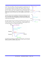
1
NanoWizard® AFM Handbook Version 2.2a 05 / 2012 © 2004-2012 JPK Instruments AG all rights reserved Contents 1. Introduction ...........................................................................................................................................1 1.1 1.2 1.3 1.4 1.5 2. About this handbook ........................................................................................................................................ 1 What is an Atomic Force Microscope? ............................................................................................................ 1 Scanning Probe Microscopy ............................................................................................................................ 2 Atomic Force Microscopy ................................................................................................................................ 3 AFM cantilevers ............................................................................................................................................... 4 Imaging modes .....................................................................................................................................5 2.1 2.2 2.3 2.4 2.5 2.6 2.7 3. Feedback and imaging control ......................................................................................................................... 5 Amplitude feedback in dynamic modes ........................................................................................................... 5 Another way of thinking about imaging modes ................................................................................................ 6 Operation ......................................................................................................................................................... 8 Phase imaging ................................................................................................................................................. 9 Force adjustment in imaging modes .............................................................................................................. 10 Applications ................................................................................................................................................... 11 Force spectroscopy ............................................................................................................................12 3.1 3.2 3.3 4. Introduction .................................................................................................................................................... 12 Data processing for analysis .......................................................................................................................... 13 Applications ................................................................................................................................................... 16 More about cantilevers .......................................................................................................................18 4.1 4.2 4.3 4.4 4.5 5. General points ............................................................................................................................................... 18 Handling information ...................................................................................................................................... 18 Cantilever types for different imaging modes ................................................................................................. 19 Tip modification ............................................................................................................................................. 20 Spring constant .............................................................................................................................................. 21 Cell imaging ........................................................................................................................................24 5.1 5.2 5.3 5.4 5.5 5.6 6. AFM in relation to other cell imaging techniques ........................................................................................... 24 Sample preparation ....................................................................................................................................... 25 Imaging modes .............................................................................................................................................. 27 Critical imaging parameters ........................................................................................................................... 28 Using the oscilloscope to optimize the imaging parameters .......................................................................... 28 Artifacts.......................................................................................................................................................... 30 Single molecule imaging .....................................................................................................................31 6.1 6.2 6.3 6.4 6.5 7. Preparation is key .......................................................................................................................................... 31 Imaging hints – intermittent contact mode in liquid ........................................................................................ 33 Imaging hints - contact mode in liquid............................................................................................................ 34 Imaging hints – imaging in air ........................................................................................................................ 35 Simple DNA protocol for imaging tests .......................................................................................................... 35 Artifacts ...............................................................................................................................................37 7.1 7.2 7.3 Tip shape issues ............................................................................................................................................ 37 Artifacts from damaged tips ........................................................................................................................... 38 Contamination ............................................................................................................................................... 39 JPK Instruments NanoWizard® Handbook Version 2.2a 1 7.4 8. Useful physics for SPM ...................................................................................................................... 41 8.1 8.2 8.3 9. The cantilever resonance .............................................................................................................................. 41 Thermal noise spring constant calibration ..................................................................................................... 41 Young’s Modulus of materials........................................................................................................................ 45 Useful chemistry and sample/tip preparations ................................................................................... 47 9.1 9.2 9.3 9.4 10. 10.1 10.2 10.3 2 Other imaging considerations ........................................................................................................................ 39 Cleaning cantilevers and tips ......................................................................................................................... 47 Silanization and APTES treatment ................................................................................................................ 48 Home made gel packs for cantilever storage................................................................................................. 49 Suppliers of AFM accessories ....................................................................................................................... 49 References......................................................................................................................................... 51 General AFM Papers ..................................................................................................................................... 51 Spring constant calibration references .......................................................................................................... 53 Books ............................................................................................................................................................ 54 JPK Instruments NanoWizard® Handbook Version 2.2 1. Introduction 1.1 About this handbook Here you can find information about the principles and methods of scanning probe microscopy. The focus is on applications in biotechnology and life science. The particular details of the JPK NanoWizard® AFM system, for both the software and hardware, can be found separately in the NanoWizard® User Manual. The aim of this document is to introduce AFM for those who are not familiar with the technique, and to provide background information and resources to aid those who are familiar with the technique to extend their knowledge of particular applications. The first sections of this handbook introduce the AFM technique, starting with the general ideas behind scanning probe microscopy. Later sections of this handbook provide more detailed information and background for more experienced users. 1.2 What is an Atomic Force Microscope? AFM is very different from optical microscopy. There are no lenses, there is no requirement for a light source to illuminate the sample, there is no eyepiece to look through; the microscope itself does not even look like a typical optical microscope. The imaging technique consists of a mechanical device, which is able to measure very small forces when atoms or molecules come close together, so it was named atomic force microscopy. Cantilevers are at the heart of an atomic force microscope. A critical part of the device called the cantilever is a plate spring, which is fixed at one end. At the other end it supports a pointed tip. The tip can be moved across a sample surface line by line, just like a lawn mower in the garden. The pointed tip is brought into contact with the sample and moved across the surface. The instrument measures the deflection of the cantilever as it scans, and from this information about the tip movement a three-dimensional image of the sample is built up. JPK Instruments NanoWizard® Handbook Version 2.2a 1 1.3 Scanning Probe Microscopy As the name suggests, the heart of an SPM is a probe that is scanned over the sample surface to build up some form of image. The type of image you get depends on the interaction that is measured by the probe. Images can be produced that reflect many different properties of the sample. The sample height information (topography), usually forms one aspect of the image, but images can also be collected that show other properties, including mechanical, electrostatic, optical, or magnetic information about the sample surface. Different probes and measurement systems are often used for the different properties, but one requirement is that the interaction between the probe and the sample is localized in some way. This is so that the measured signal is dominated by some small region of the sample closest to the tip, so that an image of the sample can be formed as the tip is scanned over the surface. This implies that the interaction must have a strong distance dependence, so that only the nearest parts of the sample contribute to the interaction felt by the tip. The range of the interaction will be one factor in the final resolution of the instrument. When the interaction has a very strong distance dependence, such as the electron tunneling current used in STM, the resolution can be good enough to “see” individual atoms. Since the measured signal should be dominated by the small region of probe and sample that are closest together, the actual probe does not need to be an isolated point. The probe can be part of some larger structure that is more convenient to mount and scan. The size of the probe can be relatively large, perhaps hundreds of microns or more, but if the interaction has a short enough range then the signal will be dominated by the very tip region of the probe, so that resolutions can still be achieved in the range from atomic distances to microns. The idea of a probe measuring a local interaction and building up an image is relatively straightforward, but the actual implementation of a system with a resolution in this range is technically challenging. Many factors came together in the development of scanning probe microscopy, including the development of piezoelectric materials that made it possible to reproducibly position and scan components with a sub-nanometer precision. The following diagram shows some of the different forms of scanning probe microscopy that have been developed. The techniques are usually named after the interaction that they measure. The list is not complete, as there are many different forms of scanning probe microscopy, and new techniques are still being developed. The information in this handbook is mainly concerned with Atomic Force Microscopy. 2 JPK Instruments NanoWizard® Handbook Version 2.2 The family of Scanning Probe Microscopes - SPMs Scanning Tunneling Microscope – STM H. Rohrer, G. Binnig (1981) Scanning Near-field Optical Microscope – SNOM Photon Scanning Tunnelling Microscope - PSTM Atomic Force Microscope – AFM G. Binning, C. Quate, C Gerber (1986) Magnetic Force Microscope - MFM Scanning Ion Conductance Microscope - SICM Scanning Capacitance Microscope - SCM Electrostatic Force Microscope - EFM Scanning Chemical Potential Microscope - SCPM Shear Force Microscope - ShFM Scanning Thermal Microscope - SThM 1.4 Atomic Force Microscopy The atomic force microscope (AFM) is one of the family of scanning probe microscopes, and is widely used in biological applications. The AFM uses a flexible cantilever as a type of spring to measure the force between the tip and the sample. The basic idea of an AFM is that the local attractive or repulsive force between the tip and the sample is converted into a bending, or deflection, of the cantilever. The cantilever is attached to some form of rigid substrate that can be held fixed, and depending whether the interaction at the tip is attractive or repulsive, the cantilever will deflect towards or away from the surface. This cantilever deflection must be detected in some way and converted into an electrical signal to produce the images. The detection system that has become the standard method for AFM uses a laser beam that is reflected from the back of the cantilever onto a detector. The optical lever principle is used, which means that a small change in the bending angle of the cantilever is converted to a measurably large deflection in the position of the reflected spot. The attractive or repulsive force between the tip and the sample causes a deflection of the cantilever towards or away from the sample. As the cantilever deflects, the angle of the reflected laser beam changes, and the spot falls on a different part of the photodetector. The signals from the four quadrants of the detector are compared to calculate the deflection signal. Most AFMs use a photodiode that is made of four quadrants, so that the laser spot position can be calculated in two directions. The vertical deflection (measuring the interaction force) can be calculated by comparing the amount of signal from the “top” and “bottom” halves of the detector. The lateral twisting of the cantilever can also be calculated by comparing the “left” and “right” halves of the detector. AFM is particularly suited for biological applications, because the samples can be JPK Instruments NanoWizard® Handbook Version 2.2a 3 imaged in physiological conditions. There is no need for staining or coating, and no requirement that the sample should conduct electrons. Therefore high resolution imaging is possible in physiological buffer or medium, and over a range of temperatures. Living cells can be imaged, as well as single molecules such as proteins or DNA. The force contrast gives 3-dimensional topography information, as well as the possibility to access other information such as the mechanical properties or adhesion. 1.5 AFM cantilevers Cantilevers are fabricated on chips What you get when you order cantilevers is a small micro-precision-machined rectangular or triangular piece of silicon or silicon nitride with a shiny surface. The minute cuboid you can see is not the cantilever itself, but the chip that holds the cantilever. Generally you need a magnifying glass to see the cantilever at the narrow side of the chip. Sometimes there are two or more cantilevers attached to the narrow edges of the chip. What you are unable to see without a good optical microscope is the tip at the end of the cantilever. Typically the tip is a few microns long, and shaped like a pyramid or a cone. The radius and angle of the end of the tip determines the imaging quality. Cantilevers can be thought of as springs. From physics lessons in school, you may recall that the extension of springs can be described by Hooke's Law F = - k * s. This means: The force F you need to extend the spring depends in a linear way on the distance s that you extend it. This linear behavior just means that if you double the deflection of the spring, the force is also doubled. The four damping springs of a car's wheels have a higher spring constant than the spring in your ball pen. The spring constants of the commercially available cantilevers vary over four orders of magnitude; cantilevers with spring constants between 0.005 N/m and 40 N/m are commercially available. You can deduce the properties of a cantilever from its outer shape. Thicker and shorter ones tend to be stiffer and have higher resonant frequencies. 4 JPK Instruments NanoWizard® Handbook Version 2.2 chip cantilever 2. Imaging modes 2.1 Feedback and imaging control The detection system measures the cantilever deflection as the tip is moved over the surface by the scanning system. It is possible to scan laterally over the surface without changing the height of the cantilever and just measure this deflection signal. This is known as “constant height” imaging, but is not the most common solution. The force applied by the cantilever depends on the deflection, so higher parts of the sample will experience higher forces in this mode. It is much more common to use some form of feedback loop to monitor the cantilever response, and adjust the height of the cantilever accordingly to take account of the changes in surface height. In this case, the base of the cantilever is moved up and down over higher and lower parts of the sample. All parts of the sample should now experience the same force, if the system is well set up, and the maximum force can be controlled. A “PI” controller is often used to control the imaging, which means that proportional-integral feedback is used. The difference between the setpoint and actual values is used to change the height position of the cantilever. There are two values to set how the height position is updated; a time constant for the integrator and a value for the proportional gain. These two values control how quickly the feedback responds to a change in sample height. The actual values need to be optimized for different imaging conditions, depending on the sample topography and scan speed for example. If a value of the cantilever deflection is selected then the feedback system adjusts the height of the cantilever to keep this deflection constant as the tip moves over the surface. Thus the microscope images using “constant force” rather than constant height. When the deflection of the cantilever is used as the feedback signal, this is usually known as contact mode imaging. 2.2 Amplitude feedback in dynamic modes There are other ways of operating the system, using dynamic modes where the cantilever vibrates, and this oscillation of the cantilever is measured rather than the static deflection of the tip. There are different ways to excite the oscillations - the cantilever substrate can be shaken directly, or a magnetic field can be used to drive the cantilever itself if it is coated with a ferromagnetic layer. In aqueous conditions, the most common technique is to drive the cantilever acoustically through the liquid. In all these cases, however, the measurement of the cantilever oscillation and control systems are similar, and the cantilever is usually driven close to resonance. In these dynamic modes, a setpoint amplitude is chosen, and the height adjusted to match this amplitude through the feedback system. In addition to the height and error signal information from this constant amplitude mode, the phase between the JPK Instruments NanoWizard® Handbook Version 2.2a 5 drive signal and the cantilever can also be measured. There are several different dynamic modes, depending on how much of the oscillation cycle the tip actually makes contact with the surface. Intermittent contact mode is widely used, and can give a combination of the benefits of the other modes. The cantilever oscillates and the tip makes repulsive contact with the surface of the sample at the lowest point of the oscillation. The lateral forces can be much lower than contact mode, since the proportion of the time where the tip and sample are in contact is quite low. There may be a higher normal force between the tip and sample when they are in contact, however. In non-contact mode the cantilever oscillates close to the sample surface, but without making contact with the surface. This mode is not so widely used, since the attractive force means that there is a possibility of the tip jumping into contact with the surface. The capillary force makes this particularly difficult to control in ambient conditions. Very stiff cantilevers are needed so that the attraction does not overcome the spring constant of the cantilever, but the lack of contact with the sample means that this mode should cause the least disruption. Another mode is possible, where the tip does not leave the surface at all during the oscillation cycle. This is something like a dynamic form of contact mode, and is usually called force modulation mode. 2.3 Another way of thinking about imaging modes The imaging modes can also be thought of in terms of the forces between the tip and surface. Generally, when two objects are brought together, the long range forces are attractive, and the force becomes repulsive when the objects are close together. The longer-range attractive forces are usually van der Waals forces and capillary forces, and then the repulsive interaction takes over at short ranges, when the objects are in “contact” and the electron orbitals begin to overlap. The situation may be a lot more complex, however, when electrostatics and other interactions from soft samples in liquid are taken into account. Broadly, though, a general curve can be drawn of the tip-sample force against distance, and the different operating modes can be matched with different parts of the curve. An example is shown, which demonstrates the main features. The curve is a general approximation, however, and different samples will have very different curves in practice. Negative force (below the axis) is attractive in this diagram, and positive force (above the axis) is repulsive. As the tip and sample approach from a long distance, the attractive force increases to some minimum in the curve. Approaching beyond this minimum reaches a relatively sharp upwards part of the curve into the repulsive regime. 6 JPK Instruments NanoWizard® Handbook Version 2.2 Contact and Force modulation modes both stay entirely in the repulsive part of the curve. In this kind of model of two objects approaching one another, there is no one point where the objects go from being “not in contact” to being “in contact”, since they interact in some way over the whole range of distances that separate them. So “contact mode” is just a shorthand for choosing a particular value of repulsive force for the feedback to use to control the height. In contact mode a single value of the force is chosen and in force modulation mode the force is varied. Intermittent contact mode moves between the attractive and repulsive parts of the curve. The maximum force perpendicular to the sample may be higher or lower than in contact mode, but this is only applied for a short part of the cantilever cycle. Therefore the sample damage and lateral drag can both be reduced compared with contact mode for some samples. Non-contact mode is the only one that stays in the attractive part of the curve, but this makes it difficult to control, so it is not often used. In liquid, the attractive part of the curve may not be so obvious, and the oscillation is heavily damped, so it is not usually possible to use it on biological samples in liquid. The ranges for the operation of the different modes also vary a lot, so the force values can overlap for different modes, but this overview shows the general operating regimes for the different imaging modes. JPK Instruments NanoWizard® Handbook Version 2.2a 7 2.4 Operation Contact mode In contact mode, the tip never leaves the surface, so this mode can be used for very high resolution imaging, such as atomic resolution of inorganic crystals or the images of protein crystals showing the subunits of the proteins. The maximum vertical force is also controlled, so the compression of the sample can be limited. The lateral forces as the tip moves over the surface can be a problem in some situations, but can actually be an advantage in other situations. The lateral deflection can give information about the friction force between the tip and the sample, and can show up areas that may have the same height, but different chemical properties. In contact mode, the setpoint value is the deflection of the cantilever, so a lower value of the setpoint gives a lower imaging force. Intermittent contact mode In intermittent contact mode, the tip is not in contact with the surface for most of the oscillation cycle. The lateral forces can therefore be much lower, and this mode can be used for imaging samples such as molecules that are not firmly stuck down on the surface, without moving them around. The cantilever is usually driven close to a resonance of the system, to give a reasonable amplitude for the oscillation and also to provide phase information. The phase of the cantilever oscillation can give information about the sample properties, such as stiffness and mechanical information or adhesion. The resonant frequency of the cantilever depends on its mass and spring constant; stiffer cantilevers have higher resonant frequencies. In intermittent contact mode, the setpoint value is the amplitude of the oscillation, so a higher setpoint value means less damping by the sample and hence a lower imaging forces. Cantilevers and spring constants Different imaging modes tend to use cantilevers with different properties. In contact mode, the deflection of the cantilever is controlled as the tip is scanned over the surface. A softer cantilever means that a lower force can be used to give the same deflection. Often lower forces give better imaging, so the softest cantilevers are generally used for contact mode imaging. Many cantilevers are available with spring constants (k) below 0.5 N/m. Stiffer cantilevers are usually used for intermittent contact mode, particularly in air. These generally have a resonant frequency of 200 – 400 kHz, and spring constants of more than 10 N/m. These stiffer cantilevers give more stable imaging in air, since the cantilever is able to break free of the capillary forces when the tip touches the sample. As there can be very low average deflection values during careful imaging, the stiffer cantilevers do not necessarily damage the surface. 8 JPK Instruments NanoWizard® Handbook Version 2.2 The mass of a cantilever strongly influences its resonant frequency and spring constant. A light cantilever with a high spring constant will have high resonant frequency. The higher the resonance frequency, the better the high speed response of the cantilever in air. Res. Freq. f = 1 k 2π m For intermittent contact mode in liquid, the capillary force is not a problem, and softer cantilevers are often used. “Contact mode” cantilevers are often used for intermittent contact mode in liquid conditions. The resonant frequencies are much lower, and the damping of the liquid around the cantilever has a strong effect on the resonance. The resonance of typical soft cantilevers in liquid is usually a few kilohertz, but in fact the cantilever is often driven at a resonance of the liquid cell or acoustic cavity in this frequency range rather than the actual cantilever resonance. The spring constant of a cantilever can be estimated from its geometry and the properties of the material it is made from. The spring constant depends very strongly on the thickness of the cantilever, however, and this can be difficult to measure accurately. If a calibrated reference cantilever is available, then the cantilevers can be pushed against one another to compare the deflection of one cantilever by the other. For soft cantilevers another option is to measure the thermal noise and calculate the spring constant. This is an attractive option, since the cantilever is not damaged by the measurement, and no extra equipment is required. These methods are discussed further in Section 4.5 2.5 Phase imaging During an AFM experiment in intermittent contact mode the cantilever is driven at some frequency in the kilohertz range (a few kHz in liquid, or a few hundred kHz in air typically). The whole cantilever vibrates with the same frequency, but depending on the conditions of the tip and sample there will be some phase shift between the drive signal and the cantilever movement measured by the lock-in-amplifier. This phase shift can be measured and displayed in a phase image. The phase signal is sensitive to properties of the tip-sample interaction, and may show up mechanical information about the sample. Adhesion between the tip and sample or other dissipation of the cantilever energy by a viscoelastic response of the sample are two mechanisms that may cause a large phase shift of the resonance. This means that sometimes in phase images two different components embedded on a topographically flat sample can be distinguished, as in the example shown here. Height and phase images of the same area are shown, with the scale bar of 1 micron in each case. In the height image, there is an area in the lower right hand corner where the texture is different. The height changes smoothly, however, and different regions can not be distinguished within it. In the phase image, there is a sharp change of phase shift at the edge of the textured area, and there is a sharply contrasting region within it. This feature is marked with an arrow in the phase image. This is typical of the case where material property differences show up in the phase, independently of the height. JPK Instruments NanoWizard® Handbook Version 2.2a 9 The quality of a phase image can be strongly influenced by varying the setpoint in intermittent contact mode. The phase should also be corrected when the cantilever is tuned at the start of intermittent contact mode imaging. There are always some offsets due to the system, which do not depend on the sample interaction. The phase should be set so that it goes through the centre of the resonance, when the tip is not interacting with the sample. Then when the tip and sample are brought together, the phase shift due to the sample can be distinguished. This operation is described for the JPK AFM and software system in the NanoWizard® User manual. 2.6 Force adjustment in imaging modes The force applied to the sample can strongly influence the quality of the image, particularly on soft samples. It is therefore essential to be informed about the current force. Contact mode Le Grimellec, C. et al. Biophys. J. If the spring constant of the contact mode cantilever is known it is easy to get information about the force applied to a sample during imaging. In the JPK NanoWizard software, the setpoint can be displayed in units of force if the cantilever has been calibrated. With this value it is possible to adjust the current force applied to the sample exactly. 75:695-703 (1998). "Imaging of the surface of living cells by low-force contact-mode atomic force microscopy” Intermittent contact mode Vié, V. et al. Ultramicroscopy In intermittent contact mode it is also possible to determine the average force applied to the sample during imaging, using the vertical deflection signal. A useful reference for this can be found in: 82:279-288 (2000). "Imaging of the surface of living cells by low-force contact-mode atomic force microscopy” The typical forces applied to a sample strongly depend on the particular application and the type of sample: Scanning of living cells 100 pN le Grimellec, 1998 1-30 nN Fritz 1994, Radmacher 1997 Nano-scribing ~ 5 nN, depending on the material Nano-manipulation < 1 nN in any case < 500 pN to move molecules in case of H-bonds ~ 100 pN to move molecules 10 JPK Instruments NanoWizard® Handbook Version 2.2 2.7 Applications Molecules and membrane surfaces The highest resolution images are usually obtained on single molecules immobilized on a surface such as glass or mica. It is possible to study protein sub-structure and organization, particularly in 2-dimensional protein crystals. This can also be successful with membrane proteins, in conditions that would not allow 3-dimensional crystallization for standard structural investigations. Long molecules such as DNA or glycoproteins can be studied to measure intrinsic properties such as the persistence length, or interactions with bound proteins. The molecules do not need coating or staining and can be imaged in air or liquid. Molecules can be studied in action, for example enzymes such as collagenase or amylase digesting their substrate. DNA One of the most important factors in high resolution imaging is the sample preparation, that the sample should be very clean and firmly adsorbed to the substrate. Protein crystal Cell imaging AFM has many advantages for cell imaging, since the cells can be imaged at high resolution in physiological conditions, in buffer or medium. Living cells can be imaged, and this has led to studies of the effects of different drugs or conditions on the cell morphology and behavior. Cells infected with parasites or viruses have also been studied. The details of the cytoskeleton are usually visible in the images of live cells, while fixed cells show the highest resolution features of the membrane surface. Many possibilities open up if the AFM can be mounted on an inverted optical microscope, so that DIC or fluorescence images can be compared with the 3-dimensional topographic information, or the maps of the mechanical properties of the cell surface. AFM and optical Other modes and interactions Apart from simply imaging, AFM cantilevers can be used in many other modes of interaction with the surface. The tip can be used to pattern the surface, move and manipulate molecules or parts of the sample, or even to dissect the sample on a nanometer scale. Nanolithography is possible, for example by applying a bias voltage and using the natural water capillary that forms between the tip and sample in air to oxidize patterns on the surface. With modified cantilever tip surfaces, molecules on the tip can be patterned onto the surface, or molecules on the surface can be picked up and moved around. The tip can be used to image normally, and then higher forces applied to cut through parts of the sample, for example to dissect a labeled part from a chromosome. There are as many applications for AFM as there are biological samples, so it is beyond the scope of this introduction to give a full picture here. The applications page for the NanoWizard® AFM and the NanoWizard® image gallery on the JPK website contain more examples of the range of AFM applications and experiments that are possible. JPK Instruments NanoWizard® Handbook Version 2.2a www.jpk.com 11 3. Force spectroscopy 3.1 Introduction The AFM is best known for its high-resolution imaging capabilities, but it is also a powerful tool for sensitive force measurements. Information about the sample is also available from measuring the changes while the separation from the surface is varied at a single point, rather than by scanning the lateral position of the tip. In this mode the base of the cantilever is moved in the vertical direction towards the surface using the piezo and then retracted again. During the motion, the deflection of the cantilever and other signals, such as the amplitude or phase in dynamic AFM modes, can be measured. This is usually called force spectroscopy. The AFM tip is able to probe an extremely small interaction area (using a tip radius in the range of 5-50 nanometers), and this gives it a high sensitivity to small forces. The study of interaction forces with the AFM has led to deeper understanding of many biological and physical processes down to the single molecule level. Simple force curves The data from an experiment is often displayed as a simple x-y plot. The height positions for the approach or retract of the cantilever are usually chosen as the xaxis, and the cantilever property that is being measured is the y-axis. This is usually the vertical deflection of the cantilever, which can give a direct measure of the interaction force. These "force-distance" plots are often referred to as force curves. The basic force spectroscopy curves can be understood by thinking about the example of a cantilever in air approaching a hard, incompressible surface such as glass or mica. As the cantilever approaches the surface, initially the forces are too small to give a measurable deflection of the cantilever, and the cantilever remains in its undisturbed position. At some point, the attractive forces (usually Van der Waals and capillary forces) overcome the cantilever spring constant and the tip jumps into contact with the surface. 12 JPK Instruments NanoWizard® Handbook Version 2.2 Once the tip is in contact with the sample, it remains on the surface as the separation between the base and the sample decreases further, causing a deflection of the tip and an increase in the repulsive contact force. As the cantilever is retracted from the surface, often the tip remains in contact with the surface due to some adhesion and the cantilever is deflected downwards. At some point the force from the cantilever will be enough to overcome the adhesion, and the tip will break free. More complex interactions Many interesting samples are not hard and incompressible, and a more general pair of approach and retract curves will include sample compression, hysteresis and more complex adhesion between the tip and surface. In liquid, there may not be an obvious snap to contact in the approach curves even over a hard surface such as mica. Over a soft, compressible sample in liquid, the force curve often shows a gradual increase in force, without the sharp onset of the interactions seen in air. It is often difficult to define a single point where the tip and sample come into “contact”, since the initial compression of the surface causes very little deflection of the cantilever. The gradient of the repulsive contact region changes as the sample is indented and the apparent stiffness may change as the structure is compressed. For thin samples on a hard surface, the linear repulsive contact regime may be seen at large deflections, as the tip may indent the sample enough to feel the supporting surface below. The contact area will change as the tip indents a soft surface, so the actual interactions involved in compression can be hard to quantify, and different points within the region will experience different levels of compression. When the tip is retracted from the surface, there is often a hysteresis seen, if the sample is not perfectly elastic, and many different adhesion responses can be observed. In some cases, the cantilever pulls the tip free in stages, such as when there are long molecules in the sample or on the tip. Extendable contacts are made between the tip and sample, so that as the base of the cantilever retracts, the tip is deflected down towards the sample until the force is strong enough to break the contacts. Different molecules or parts of the sample may adhere and each part may be broken separately, or together. These situations produce a variety of adhesion events, and successive force curves can show very different responses. The force curves are often repeated at different locations to build up a map of the tip-surface interaction, or repeated many times at the same point to give a full statistical understanding of the interaction. 3.2 Data processing for analysis The most direct way to plot the data shows the movement of the piezo during the force curve (as a distance) against the deflection of the cantilever. The deflection is measured by an optical beam deflection setup which delivers an electrical signal (in Volts, as the signal from the photodiode) that is proportional to the cantilever deflection. In the example below, Approach (red) and retract (blue) curves are both plotted on the same axes. JPK Instruments NanoWizard® Handbook Version 2.2a 13 Typical interaction for an uncoated hydrophilic cantilever in air approaching a hard incompressible hydrophilic surface (e.g. glass or mica). Hydrophilic surfaces are covered with a thin water layer in ambient conditions. These layers join when the tip and sample are close together, forming a capillary neck between them and hence a strong adhesion. Calibration of the cantilever deflection F=-k*x The deflection of the cantilever spring is directly proportional to the tip-sample interaction force, but there are two measurements required to convert the photodetector signal into a quantitative value of force. The first stage is to calibrate the distance that the cantilever actually deflects for a certain measured change in photodetector voltage. This value depends on type of cantilever, but also on the x = cantilever deflection (units of distance) k = spring constant optical path of the AFM detection laser, and will be slightly different each time the cantilever is mounted in the instrument. Once the deflection of the cantilever is known as a distance, the spring constant is then needed to convert this value into a force, using the well-known Hooke's law. F = deflection force A force curve between a plain cantilever tip and a bare hard substrate is used to determine the sensitivity of the experimental setup. This is a measurement of the deflection of the tip in nanometers for a given movement of the detection laser on the photodetector. The repulsive contact region, where the deflection rises steeply upwards, is linear for a hard surface and tip. Therefore the software can easily determine the factor for converting Volts into nanometers. This measurement can then be used for calibrating the applied forces when the samples of interest are investigated. The sensitivity can then also be used to set the oscillation amplitude in intermittent contact mode as actual nanometers of oscillation. The gradient chosen for sensitivity measurements and the baseline offset for the deflection are both marked on this plot. Since the hard repulsive interaction regime is used for the sensitivity measurement, the force curves are often actually done at the end of the experiment to avoid damaging the tip. The example above shows the two regimes useful for calibrating the deflection. When the cantilever is far from the surface, the interaction forces are virtually zero (the flat part of the curve on the right hand side). This offset , which may be due to the initial settings of the equipment, or to thermal drift, should be subtracted from all the deflection data in order to calculate the true interaction force. 14 JPK Instruments NanoWizard® Handbook Version 2.2 On a hard surface: Change in cantilever deflection = change in piezo height The other linear region, on the left hand side of the plot, is where the tip is resting on the surface. If the surface is not compressed by the cantilever forces, then the change in the piezo height (known from the height calibration in nm) is equal to the cantilever deflection (measured from the photodiode in Volts). The sensitivity is the conversion factor (nm true deflection per Volt measured deflection) needed to convert the photodiode deflection into units of length. The example from above has been shifted here to give a zero baseline. The sensitivity (measured from the curve above as 22 nm/V) has been used to convert the deflection into units of length (nm). Approach Retract The deflection values here are now ready to be converted to units of Force (N). Correction of the height for the cantilever deflection The plot so far has used an x-axis of the cantilever height directly measured from the piezo position. For quantitative analysis of indentation or stretching, however, the cantilever is obviously deflected from its equilibrium position. The deflection should be taken into account to extract the true tip position relative to the surface. The deflection can then be plotted against the tip-sample separation, rather than the piezo height. Now that the deflection is in units of length, it can be subtracted from the piezo height at each point to correct for the tip position. After the sensitivity conversion, the straight line part of the repulsive interaction (left hand side of the curve above) has a gradient of 1, since this is the basis of the sensitivity calculation. Once the height scale is corrected, this becomes a vertical line (as seen in the curve below). This is because the tip-sample separation remains constant at zero, and the action of the piezo movement merely increases or decreases the force. The example from above has had the x-axis corrected for the tip deflection. The x-axis is now the true tip-sample separation, rather than the piezo height measured directly. For quantitative force measurement, the spring constant of the cantilever must be calibrated, so that the nanometers deflection of the cantilever can be converted into actual force values. There are various different ways of calibrating spring constants of cantilevers, depending on the equipment that is available. See Section 4.5 for more details. The example above has had the deflection multiplied by the spring constant to express the deflection as a force and would now be ready for analysis. JPK Instruments NanoWizard® Handbook Version 2.2a 15 3.3 Applications There are a huge number of potential applications of force spectroscopy, ranging from nano-mechanical investigations of elastic properties to protein unfolding and investigations of single chemical bonds, so only a brief overview is possible here. Virtually any sample can be studied using force spectroscopy, and different interactions or tip coatings and shapes will all give complementary information about the sample. Molecular interactions When molecules are attached to the tip and/or the sample, the stretching, unfolding or adhesion of single molecules can be studied. Long chain molecules, such as DNA or dextran can be stretched between the tip and the sample. The stiffness, persistence length and internal molecular transitions can be studied. The melting transition in DNA can be seen as the backbone rearranges under raised tension. Molecules with complex 3-dimensional structure, such as many proteins, can be unfolded in a controlled way so that the structural units can be investigated. Titin and bacteriorhodopsin are examples of proteins that have been intensively studied. Membrane proteins can be pulled out of the membrane, and the “popping” out of individual alpha-helices has been seen. The adhesion can be measured between molecules attached to the tip and to the sample. These can be antibodies and antigens or other receptor-ligand pairs. The adhesive forces can be measured and mapped over the surface, and information extracted about the energy and kinetics of the binding. These techniques have also been applied to the binding between complementary and mismatched DNA strands. Cellular mechanics and interactions The viscoelastic response of cells can be studied by using the cantilever to indent the cell. On living cells, the changes in mechanical properties can be seen as the cell divides, or when drugs such as cytochalasin, which disrupts the cytoskeleton, are added. Mechanosensitive cells such as osteoblasts or ear cells can be stimulated with the cantilever, and the response monitored. Adhesion maps over the surface are also possible to investigate the distribution of receptors. The following table gives an overview of some interactions, and the part of the force curves that they are measured in. 16 JPK Instruments NanoWizard® Handbook Version 2.2 Approach Tip far away No interaction (10 - 100 microns) Tip approaching (few microns) Tip close to surface (nanometers to atomic distances) • Electrostatic forces Long-range interactions from adsorbed molecules, e.g. polymer brush • • • • • • Van der Waals Capillary forces (in air) DLVO/screened electrostatics (in aqueous solutions) Chemical potential Magnetic Solvation forces (water layering) Contact Tip indenting sample • Stiffness (Young's modulus, elastic response) • Viscoelastic response (variable rates or indentation depth) Measurement of active forces (e.g. generated by cells) Retract Tip lifting off surface Adhesion: (few atomic distances to • Non-specific (including chemical affinity, surface coatings) nanometers) • Ligand-receptor (e.g. antibody-antigen) • DNA hybridization (e.g. matched or mismatched pairs) • Cell surface interactions Tip further away (nanometers to hundreds of nanometers) Stretched molecules between tip and surface: • Protein unfolding, pulling out of membranes • Entropic elasticity • DNA stiffness, structural transitions and "melting" • Other conformational changes in stretched molecules, e.g. chair-to-boat transition in sugar rings Cell Other stretched attachments e.g. membrane tethers formed on cells Tip far from surface (1-5 microns) Connections broken between the tip and surface, no further interaction. Adhesion strength can be measured between attached molecules and the surface when the attachments break. Overview of some of the interactions measured at different points during a force spectroscopy cycle. Receptorligand JPK Instruments NanoWizard® Handbook Version 2.2a 17 4. More about cantilevers 4.1 General points The terminology concerning cantilevers can be confusing. The large piece of silicon is called the “chip”, and is a support for handling with tweezers and for gripping with the cantilever holder spring. The “cantilever” itself is generally in the range of 100 µm long. The “tip” is the projection that is used for imaging, and is usually placed at the very end of the cantilever. Often, however, the term “cantilever” is used when the “chip” or “tip” is actually meant. Normally the tip attached to the cantilever cannot be seen without a good microscope. Depending on the material and application, the tips can be shaped like an Egyptian pyramid, or longer and cone shaped. The cantilever itself is usually either rectangular or triangular in shape, such as the examples shown below. chip cantileve View from above tip cantilever Magnified view from the side Many types of cantilevers and tips are available for different applications. Most are microfabricated from silicon or silicon nitride, and batch fabrication of probes gives reasonably consistent physical properties. AFM cantilevers generally have a metallic coating on the back side to increase the reflectivity. Aluminium is a common choice because of its high reflectivity, but gold is often better for cantilevers that will be used in liquid, because it is so chemically inert. Other coatings can be used to give magnetic sensitivity, or to modify the actual tip region to produce particular chemical interactions with the sample. 4.2 Handling information Cantilevers are expendable items and have to be replaced regularly. The lifetime of AFM cantilevers strongly depends on the way they are handled. The price of a single cantilever starts in the range of 15 EUR (Summer 2003) up to hundreds of Euros for special application cantilevers. Cantilevers are usually delivered in plastic packages called “gel packs” of up to 50 pieces. The chips are held on a soft and adhesive polymer layer. Movement and damage during delivery and storage is prevented, but they easily can be released from the adhesive layer with a pair of tweezers. Larger amounts of cantilevers are often delivered as a whole wafer in nitrogen-filled plastic containers. In this case no 18 JPK Instruments NanoWizard® Handbook Version 2.2 adhesive layer is required for storage, since the chips are held in the wafer. Gelpacks can be bought from cantilever manufacturers or can be home made for storing tips after delivery Instructions for making gel-packs are given later in this document (see Section 0). The cantilever and tip are both susceptible to damage If the tip is damaged, the tip radius generally increases. With worn or contaminated tips, the image resolution will be lower and the images may have serious artifacts (see the discussion in Section 7). Damage to the cantilever arm may also cause problems for imaging. Handle the cantilever chips carefully: • Do not touch the cantilevers with fingers. Use tweezers to handle them. • Do not drop the cantilever chips. The cantilevers may break off the chip. • Only open the cantilever package when necessary. • Only open the cantilever package in a clean environment. • The tips may also be damaged through inappropriate scanning conditions: • Too high gain parameters may lead to a damage of the cantilever tip. • Too high setpoint values in contact mode may damage the tip. • Too low setpoint values in intermittent contact mode may damage the tip. 4.3 Cantilever types for different imaging modes The geometry and the material of the cantilever both contribute to the properties that make a cantilever suitable for any particular imaging modes. Most cantilevers are designed for either contact or intermittent contact mode. The shape/geometry of the cantilevers influences the properties that qualify the cantilever to be a contact or an intermittent contact one. The chip and the tip do not have any influence on this, however. Contact mode For contact mode, AFM cantilevers with low spring constants are required. As tip wear is inevitable in contact mode, any additional tip coating will be subject to damage. Use silicon nitride tips or diamond coatings if a reliable tip shape is required. Silicon nitride tips will deliver best results for soft materials. • Low force constant • “Soft cantilevers” • Low resonant frequency • Longer and thinner Using cantilevers that are too stiff (such as most of the cantilevers designed for intermittent contact mode) can lead to applying high forces to the sample. On hard samples, the tip can then be damaged very easily. On soft samples the tip can damage the sample easily. There are some cantilevers that are strongly not advised for use in contact mode. Cantilevers with especially sharp tips such as EBD cantilevers (see below) and sharply edged cantilevers are so delicate that their very easily be damaged if used in contact mode. JPK Instruments NanoWizard® Handbook Version 2.2a 19 Intermittent contact mode For intermittent contact mode AFM in air, stiffer cantilevers with resonance frequencies above 100 kHz are required (resonance frequencies between 200 and 300 kHz deliver the best results). Some intermittent contact mode cantilevers are available with lower resonance frequencies, in the 100 kHz range. These can be useful for AFM instruments from some other manufacturers that are not able to use such high frequencies as the NanoWizard® AFM. The disadvantage is that the scanning speed must be lower to reach the same resolution. • High force constant • “hard cantilevers” • High resonant frequency • Shorter and thicker Res. Freq. f = 1 k 2π m It is possible to use softer cantilevers (such as the ones designed for contact mode), but it is more difficult to establish a stable feedback with them. The problem in air is that the vibrating cantilever has to cope with a thin water layer which is always present on a sample surface at in ambient conditions. The strong adhesion of the water layers on the sample and tip can trap the cantilever on the surface, making the imaging unstable. If the humidity of the environment is reduced, this can improve the situation, however. For intermittent contact mode in liquid, softer cantilevers are often used, because when the cantilever and surface are immersed in liquid there is not this problem with the surface water capillary layers. So for intermittent contact mode in liquid, often “contact mode” cantilevers are actually used. General points Both silicon and silicon nitride cantilevers are available form many suppliers, but a reflective back surface coating is recommended for superior feedback. The unique chip holder of the NanoWizard® allows you to use tips from most manufacturers, and probes are available from our website. The instrument was performance tested with probes from NanoWorld®, NanoSensors®, Veeco®, Olympus® and Mikromasch®. The examples of technical data given below are from the NanoWorld® cantilevers CONT and NCH. The listing is just to give a comparison for typical values. Technical data Typical value Range Thickness Mean Width Length Force Constant Resonant Frequency 2 µm 50 µm 450 µm 0.2 N/m 13 kHz 1.5 - 2.5 45 – 55 445 – 455 0.07 - 0.4 9 - 17 Technical data Typical value Range Thickness Mean Width Length Force Constant Resonant Frequency 4 µm 30 µm 125 µm 42 N/m 320 kHz 3.5 - 4.5 25 – 35 120 – 130 21 – 78 250 - 390 Contact mode Intermittent contact mode 4.4 Tip modification For many applications, the tip is modified chemically or physically to give particular 20 JPK Instruments NanoWizard® Handbook Version 2.2 properties. There are many different options, depending on the particular application, but a couple are introduced here. Hydrophobic cantilevers Hydrophobic tips can be used to image hydrophilic surfaces (e.g. proteins) under high-humidity conditions with small forces and thus high resolution. The adhesion between hydrophobic and hydrophilic surfaces is lower than between similar surfaces, so the sample disruption should be less. Silanization is one method to change the chemical groups on the surface of the cantilever, and make it more hydrophobic. An example of a silanization protocol is given in this handbook, see Section 9.2. EBD tips Electron beam deposited (EBD) tips are AFM tips that have been modified to grow a narrow tip-on-the-tip. Normally shaped silicon intermittent-contact cantilevers are modified in scanning electron microscopes. The electron beam focused on top of the tip deposits a small column of carbon, leading to a tip with narrow radius and high aspect ratio. The carbon is from the hydrocarbon contamination in the vacuum chamber of the SEM. The high aspect ratio of the tip is one advantage of this method, and allows imaging of structures such as grooves or troughs, that are not imaged well by tips with conventional shapes. The amorphous carbon surface may also be less adhesive than the bare silicon tips for imaging samples such as proteins. Each tip must be individually modified, however, and this is not practical for most AFM users on grounds of either access to equipment, or cost to purchase such tips. Knapp, HF, Wiegräbe, W, Heim, M, Eschrich, R, Guckenberger, R. Biophys. J. 69 (1995) 708-715. "Atomic force measurements and manipulation of Langmuir-Blodgett films with modified tips” 4.5 Spring constant Background information The analysis of force curves uses force against tip-sample separation. This means the vertical deflection signal from the detector has to be converted from Volts into Newtons, and the z-position signal needs to be corrected for the deflection of the AFM tip along the same axis. The spring constant calibration (N/m) is generally the most difficult part of the calibration. There are various different methods to calibrate the spring constant of an AFM cantilever, and unfortunately all of them have significant problems. If experiments are compared where different methods are used, sometimes differences of 10-20% can be seen. The methods are reasonably consistent if they are used carefully, so it is often good to pick one particular method and calibrate all cantilevers as consistently as possible. This means the data from different cantilevers can be combined well to give good statistics. Then it is just important to realize that there will be some systematic difference between the results from different methods. JPK Instruments NanoWizard® Handbook Version 2.2a 21 The thermal noise analysis is becoming the main standard for AFM experiments, because it is available in liquid, online during the experiment, through a fast, automated software analysis. There are some difficulties in the theoretical analysis due to cantilever shape, liquid damping, etc., but the convenience and speed means it is now very widely used. Calculation from cantilever geometry Cantilevers purchased by manufacturers are generally delivered together with a data sheet, which gives the cantilever specifications. Properties such as the spring constant have generally been calculated from the cantilever geometry, and have not been experimentally measured. Calculation of spring constant E⋅wt k= 4 l k Calculation of resonant frequency f f = 3 (1.8751) 2 t ⋅ 2 2π l E w t l ρ E 12 ρ Note that the force constant is independent of the mass of the cantilever, but the resonance frequency is not. Typical values for silicon; E<110> = 168.1 GPa) and ρ 3 -3 Si = 2.33 · 10 kg m 22 JPK Instruments NanoWizard® Handbook Version 2.2 Young’s modulus width thickness length mass density Measurement of the spring constant using a reference cantilever When a reference cantilever with a known spring constant kr is available, other cantilever spring constants kc can be calculated by measuring the slope of the repulsive contact part of a force-distance curve. The two cantilevers must be placed over each other, and the deflection of the unknown cantilever measured as it is pushed against the reference cantilever. This calculation is most accurate if the two cantilevers have similar values of k. If sr is the slope measured on the reference cantilever, and ss is the slope measured on a solid support (e.g. a piece of glass or mica), then the calculation is: Hinterdorfer et al. PNAS 93 (1996) 3477-3481. “Detection and s k c = k r s − 1 sr localization of individual antibodyantigen recognition events by atomic force microscopy” Ideally, the two cantilevers are brought in contact with their very tips. If there is a significant offset away from the end of the reference lever a correction needs to be made: kcorr L = kc L − ∆L 3 , where L is the length of the reference lever and ∆L is the offset away from the end. Measurement of the spring constant using the thermal noise It is also possible to measure the spring constant of a cantilever by looking at the thermal noise spectrum. The possibility to measure the thermal noise and calculate the spring constant is offered in the JPK SPM software, so more information on the method can be found in the NanoWizard User manual. The theory for the thermal noise calibration can be found in this Handbook in Section 8.2. JPK Instruments NanoWizard® Handbook Version 2.2a 23 5. Cell imaging The AFM has many advantages for cell imaging because of the high resolution and the ability to work in physiological conditions and even on living cells. Cells are however at the extreme end of samples imaged with the AFM, since they are so large and soft. Living cells are particularly challenging, since the cell itself may react to the imaging, and the stiffness is much less than for fixed cells. This section gives some information to help get started with cell imaging, and recognize the different effects that are seen when imaging living and fixed cells. There are some important considerations when designing cell-imaging experiments, such as whether the cells are adherent or not, whether they should be fixed or living, imaged in contact mode or intermittent contact mode and which particular cantilevers suit the experiment. Additionally, one must be aware of the potential artifacts that may arise during cell imaging, some of which are similar to those observed in AFM images of other samples, some of which are unique to the scanning of cells. 5.1 AFM in relation to other cell imaging techniques Cells can be visualized by a number of different techniques, each generating different information about cell structure and/or function. Obviously the fundamental requirement of any imaging technique is that contrast is somehow generated. In terms of conventional optical microscopy this may be due to a difference in material density (phase contrast), curvature (DIC) or with fluorescent microscopy the emission of specific wavelengths of light from fluorophores compartmentalized in specific locations Contrast in atomic force microscopy imaging can be generated by a number of sample properties. Topographic images from measuring the z-piezo movement are based on height differences within a sample. An error signal image will highlight edges within the sample and in intermittent contact mode the phase image can provide contrast based on material properties. Consequently, AFM imaging of cells generates structural information. This leads to a number of possibilities in experimental design. Large-scale cellular movements can be monitored by imaging living cells over time. Surface structure may be identified or the effect of certain treatments on specific structure can be investigated. A major consideration when imaging cells with the AFM is the identification of functional components within such structures, given the heterogeneity of the cell surface in terms of protein composition and distribution. Consequently, while AFM imaging of cells can generate novel information, the combination of AFM with other light microscopy techniques expands the scope of possible experiments from structural studies, to structure/function studies. 24 JPK Instruments NanoWizard® Handbook Version 2.2 5.2 Sample preparation Substrate choice and cell attachment For high resolution imaging of isolated molecules, mica is the support of choice, because it provides such a flat background. However, for cell imaging, good quality glass is sufficiently flat and has optical properties far superior to those of mica. For the combination of light microscopy and AFM imaging, the use of a coverslip as a support can give the best results, but only if the coverslip is mounted in a sufficiently stable holder, such as the BioCell™ available from JPK. Otherwise the thin glass coverslip will not be mechanically stable enough, and fluctuations/vibrations will be seen in the images. When using the BioCell for simultaneous light microscopy and AFM imaging, the choice of objective should not affect AFM quality and the use of oil or water immersion lenses should not introduce vibration into the system. In many cases cells will naturally adhere to glass or mica and no special surface treatment is necessary. However, with non-adherent samples such as red blood cells, yeast, bacteria etc the cells must be attached to a substrate before imaging. When imaging small structures, such as single molecules, many surface treatments can generate structures that mask the objects of interest. In the case of cells, however, this is not a problem as the size of the cells will be considerably larger than the deposited surface layer. One standard approach is to coat the desired substrate (i.e. mica or glass) with poly-L-lysine. Poly-L-lysine is a positively charged polymer which adsorbs very well to negatively charged glass or silicon dioxide leading to positively charged surfaces. Surface coating with Poly-L-lysine has been used to attach both cells and proteins to glass or mica. Poly-L-lysine coating protocol: Incubate surface under 10 mg/ml Poly-L-lysine (Mr 1000-4000) for 1-5 minutes. Wash the surface with water and dry under nitrogen. Incubate coated surface with sample of cells in suspension until cells settle and stick to surface (5 – 10 minutes), gently rinse with relevant buffer/media. Living or fixed cells? The decision on whether or not to fix cells will be influenced by the experimental question to be asked. There are a number of circumstances under which it is either recommended or necessary to fix cells before imaging. If high resolution images of the cell surface are required then fixation of the cells will lead to a stiffening of the cell surface and an increased attainable resolution, as determined by the nature of the atomic force microscope. Additionally, in many experiments where AFM is to be combined with fluorescence microscopy there will be a need for fixation to allow fluorescent labeling. On the other hand, fixation is not appropriate when in situ experiments are to be performed, when the object of the experiment is to investigate some dynamic process or when imaging is to be combined with elasticity measurements. Cell fixation protocol: Wash cells with PBS (containing 2+ 2+ Ca /Mg ) and add sufficient glutaraldehyde (2% in PBS 2+ 2+ containing Ca /Mg ) to cover the surface. Incubate for 45 seconds, remove glutaraldehyde and add paraformaldehyde (4% in PBS 2+ 2+ containing Ca /Mg ), incubate for 20 minutes. An optimal fixation protocol will avoid dehydration of the cells, as this leads to significant changes in surface structure. Additionally, it is desirable to avoid background fluorescence from the fixation protocol and to maximize fixation of structures to enhance AFM imaging. One approach that meets these criteria involves using a short fixation in glutaraldehyde followed by an extended incubation in paraformaldehyde. Care must be taken to wash cells thoroughly after fixation as residual fixant can make the surface sticky and cause problems during scanning. JPK Instruments NanoWizard® Handbook After removal of the paraformaldehyde solution, wash cells thoroughly (at least 5 x) with PBS. Fixed cells can be stored for a week (or sometimes more) in PBS, but cells should not be allowed to dry Version 2.2a out at any stage. 25 Typical images of living cells Living fibroblast cells The predominant feature of living cells scanned in contact mode is the subsurface cytoskeleton (deflection and height images shown) Typical images of fixed cells Fixed fibroblast cells Fixation of the cells leads to more detailed information of smaller surface (membrane) structures cytoskeleton (deflection and height images shown) Choice of cantilever The selection of the correct cantilever is critical for imaging cells. Selection of which spring constant a cantilever should have will depend on which imaging mode is to be used. Often very soft cantilevers are used for cell imaging, in order to minimize the force. Sources of deflection drift, such as loss of liquid due to evaporation, should also be minimized or the user will have to make more adjustments to maintain a constant force. These considerations always exist, but are more important when the force must be reduced as much as possible. The use of unsharpened, as opposed to sharpened cantilevers is recommended – particularly for imaging living cells. The potential achievable resolution is generally reduced by using an unsharpened cantilever, but for cell imaging the softness of the cell surface will limit the resolution before tip size becomes an issue. The use of unsharpened cantilevers reduces the chance of damaging the cell surface. For simultaneous fluorescence and AFM imaging it is recommended that a silicon cantilever without a surface coating is used. The heat from the fluorescence lamp leads to a deflection of the gold-coated silicon nitride cantilevers, as these levers are only coated on one side. If this happened during a contact mode scan there would be a significant increase in force applied to the sample while the fluorescent shutter was open. If the fluorescent images are taken between AFM scans, then this is not such a problem, as the cantilever can be lifted off the surface while the fluorescence shutter is open. 26 JPK Instruments NanoWizard® Handbook Version 2.2 5.3 Imaging modes The two main modes used to image cells are contact mode and intermittent contact mode. The choice of mode will depend, in part, on user preference, but there are some indicators for which will be the best choice. Contact mode Pros Intermittent contact mode Enhances visualization of subsurface cytoskeletal structures in both living and fixed cells Less lateral disruption during the scanning process Better suited for the imaging of cells with steep edges, i.e. high cell body or dendrites Less predominance of submembranous structure (for imaging of features other than subsurface cytoskeleton) Allows faster scan speeds on flatter cells Phase images available showing material properties The amplitude may remain quite constant even if the cantilever bends somewhat due to material adsorbing, for example. This would cause a force offset in contact mode, but not immediately in IC mode. Cons Comments Flexible objects will move laterally, in the scan direction (this will happen in all imaging modes but is exacerbated in contact mode) Responds less well to steep height changes such as sides of dendrites or the side of the cell body, which can complicate imaging whole cells The user must monitor the scan closely to ensure that the imaging conditions remain optimal and the applied force does not increase too much due to deflection drift More susceptible to complications due to a sticky sample or substrate In contact mode the applied force is directly related to the spring constant of the cantilever and the deflection setpoint. A softer cantilever (lower spring constant) and a lower setpoint value will apply a lower force and should therefore in general give better imaging, particularly for living cells In intermittent contact mode, the applied force is not so directly related to the spring constant of the cantilever, since the imaging sensitivity depends on the resonance properties of the cantilever. A slightly stiffer cantilever may have a better resonant behavior and hence give more sensitive imaging. A higher resonance frequency will also enable faster imaging. JPK Instruments For soft cantilevers with low resonant frequencies, the scan speeds may be rather limited, since the data collection rate can be in the range of the oscillation frequency for soft cantilevers. The feedback system will require several oscillation cycles to accurately determine the amplitude of the oscillation. NanoWizard® Handbook Version 2.2a 27 5.4 Critical imaging parameters Cantilever selection Cantilevers with a spring constant between 0.01 N/m and 0.06 N/m can be used for contact mode imaging of fixed cells. For contact mode imaging of living cells it is better that the spring constant is as low as possible (0.01 – 0.03 N/m). The softest cantilevers will be more susceptible to oscillations during scanning and may require that lower gains are used. Intermittent contact mode cantilevers can be somewhat stiffer, with a spring constant of around 0.3 N/m. Triangular cantilevers are better than springboard cantilevers for intermittent-contact mode imaging of cells. Setpoint selection The selected set point should be just sufficient for the cantilever to stay in contact with the surface. The set point should also be monitored over the course of the scan to ensure that the applied force does not increase due to deflection drift. Too high a force will lead to excessive displacement of surface structures in the scan direction or tearing of the cell surface (see image to the right). Too low a force will mean that the cantilever will not follow the contours of the cell sufficiently well. (Note – remember that increasing the setpoint in contact mode applies more force, while in intermittent contact mode it corresponds to reducing the force, since it is an amplitude) Scan rate The line scan rate will mostly depend on the structure of the cells to be imaged. Imaging of flat, well spread cells such as fibroblasts or endothelial cells will mean that scan speeds of up to 5 Hz can be used. However, with cells that have a high cell body or other high features that have steep gradients at the edges, a significantly slower scan speed may be required (even as slow as 0.2-0.3 Hz for some living cells or cells that do not adhere well). If the scan speed is not reduced in these cases the tip will fail to follow the surface correctly – see image to the right. The tip can be forced to follow the surface by increasing the applied force, however, this will disrupt other structures at the surface of the cell – using a slower scan rate achieves the same result without having a detrimental effect on other features within the scan. Error signal image of a fixed cell imaged at too high scan rate in contact mode Drive amplitude in intermittent contact mode When working in intermittent contact mode it is also important to set the drive amplitude to an appropriate value. Too high a drive amplitude may lead to damage of the cell as the cantilever drives into the surface (this will be apparent as the cell will be pushed in the scan direction), too low a drive amplitude and the cantilever may stick on the surface rather than freely oscillating. Generally a larger amplitude is required for cell imaging than for other samples, such as single molecules. A free amplitude of around 50 – 100 nm is a good starting range, though this may need to be optimized for different cell types, depending how sticky or soft they are. 5.5 Using the oscilloscope to optimize the imaging parameters 28 JPK Instruments NanoWizard® Handbook Version 2.2 The oscilloscope in the JPK SPM program can aid in selecting the correct parameters for optimal imaging (see also the main NanoWizard user manual, with details of the software interface). By viewing the trace and retrace line scans in the oscilloscope during scanning, it is possible to maintain the force applied to the surface at a minimum. By displaying the trace and retrace line scans of the height channel in the oscilloscope the user can monitor how closely the two match. Obviously if the trace and retrace match exactly then the tip is tracing over the surface of the cell without displacing any structures. To the right is an example of a good match between trace and retrace during scanning of a cell. To find the minimum force required to track across the surface of a cell, the force should be reduced by changing the set point until the trace and retrace lines no longer overlay in the oscilloscope. To determine the point where this happens, one should note how well the trace and retrace scan lines overlap at the bottom of any steep edge. In this example trace is in bright red and retrace in dull red- it can be seen that in the retrace line the tip has not followed the edge of the cell down to the glass, but has instead slightly drifted away. At this point one could try and increase the gains and decrease the force until oscillations are noticed. This can allow the use of a lower force as increased gains will result in better tracking of the tip over the surface. The other option is for the user to reduce the scan speed. If the force is reduced too far the scan lines will differ more and more at the edges of the cell until the tip loses the surface entirely. When the oscilloscope looks as it does to the right it will be obvious in the scan that the tip is not properly tracking the surface (see error signal image below, black arrows). If the force applied to the surface is too high then structures will be displaced in the scan direction. This can also be detected in the oscilloscope. Usually the structures that start to move if the applied force is too high are flexible structures. The trace and retrace scan lines in the oscilloscope show these structures moving in the direction of the scan. JPK Instruments NanoWizard® Handbook Version 2.2a 29 It can happen that the force applied to the cell is such that the tip starts to drift away from the surface at the edges (see arrows in image on the right) while still displacing a structures (blue circles). It may be that the structures in question are extremely flexible and will always be somewhat displaced. However, the user could try either a) increasing the gains, or if this leads to oscillations b) decreasing the scan speed and then decreasing the force. In the image to the right some examples of scan faults can be seen. The image presented here is an error signal image, 25 µm x 25 µm, taken in contact mode in the trace direction. The black arrows indicate areas of the scan where the tip was not tracking over the surface due to too low an applied force. The white arrows indicate some of the areas where protrusions have been displaced in the scan direction. At the top of the image a red arrow indicates an unavoidable tip artifact, where the edge of the tip has been imaged as it slides down a steep surface. 5.6 Artifacts General artifacts arising from normal tip geometry, damaged tips and contamination are described in Chapter 7. However, there is an additional artifact that should be mentioned in the context of cell imaging. Imaging of cells can be complicated by the height of the cell body, particularly if the cell body is significantly higher than other regions of the cell or substrate. If a comparatively high structure is located under the legs of the cantilever, then the cantilever can interact with the high features before the tip reaches the lower parts of the surface. This artifact can also occur if there are many dead, rounded cells in the sample. To avoid interference from such structures the user should ensure that movement of the cantilever does not bring the legs into contact with any dead and rounded cells. If the cells to be investigated have large height differences and an image cannot be obtained with out this artifact present then special cantilevers with a long tip should be used, such as EBD tips (see Section 4.4). 30 JPK Instruments NanoWizard® Handbook Version 2.2 6. Single molecule imaging 6.1 Preparation is key The AFM is well suited to biomolecular imaging, because of the high resolution and the ability to work in liquid. For high resolution imaging, however, the setup needs to meet high standards across all areas – in the sample preparation, cleanliness, and of course in the hardware and drift or vibration reduction. When imaging cells, contamination on the nanometer scale has a negligible effect on the imaging. When imaging single molecules, any contamination will be visible in the images, and may completely obscure the molecules that are intended for imaging. Start by making sure everything is clean • • • • • • Keep all tools (substrate, cantilever, cantilever holder, tweezers, pipettes, pipette tips) as clean as possible, if possible sterile. Items that can be cleaned should be cleaned in an ultrasonic bath and rinsed in ethanol and milli-Q water and blown dry. The best results are often obtained when sterile disposable plasticware is used for preparing and storing samples and buffers. Keep all chemicals (buffers, milli-Q water, cleaning liquids like ethanol) as clean as possible. Keep ultrapure water and low-to medium salt buffers in the fridge. Try to avoid using stock solutions directly – pour enough for one experiment into a separate sterile container and close the stock solution immediately. Make up buffers fresh whenever possible, filter before use with a syringe filter. If anything needs drying, use a nitrogen cylinder with a suitable gas regulator to blow the object dry (but make sure that the nitrogen is filtered and comes out of a clean tube). This removes the liquid droplets from the surface, rather than allowing them to dry onto the surface and leave all the contaminants. Basic lab equipment Syringe filters Use a good sample substrate and mount it carefully Generally, for imaging single proteins the substrate mica works best. The surface is so flat that even the smallest features can be seen on the large, molecularly flat regions, and it is easy to obtain a really clean surface by cleaving the mica. The mica surface is highly hydrophilic, and negatively charged in aqueous solutions. HOPG (highly oriented pyrolitic graphite) is another possibility, for molecules that will stick to a hydrophobic surface. This also has molecularly flat terraces, although they tend to be smaller and show more frequent step edges. A piece of high quality silicon wafer is also a possibility for hydrophobic samples, if this is from a good source and well handled. This generally has to be chemically cleaned before use. Almost all other surfaces have a higher roughness, and so are only suitable for larger molecules or complexes. Coverslips generally have the smoothest surface of glass samples, and can be conveniently cleaned with water and ethanol, although this may not be enough to remove all contamination. JPK Instruments NanoWizard® Handbook Version 2.2a 31 The mechanical stability of the sample mounting is also critical for high resolution imaging. A solid base, such as a metal stub or glass microscope slide is a good start. The mica or other substrate should then be glued with a crosslinking glue or epoxy. If the imaging is only in air, then solvent-based glues like superglue (cyanoacrylate based fast-setting glue) are a convenient alternative. Superglue is not stable in water, and will swell, become soft and lose material into the liquid. So even if the liquid should not come into contact with the glue, it is not recommended. A 2-part epoxy makes a stable, solid bond that will not be affected by contact with liquids and will not drift or move with time. Although this is usually slower than superglue, it is worth the extra time preparing the substrates, to avoid later timeconsuming experiments being contaminated. Fast setting epoxies (for instance, 5minute Araldite Rapid) give good results. UV-setting glue is also a good alternative if a UV lamp is available – this gives good mechanical results, fast setting and very good optical properties (for example the Optical Adhesive range from Norland). Double-sided tape is never recommended for high resolution imaging! When the tape is stuck, there is usually some shear on the surface. The elastic polymer components tend to relax back over time, giving large drift over hours or even days. The results can be reasonable if the tape is stuck very carefully, but it is not worth preparing precious samples using this kind of mounting, only to discover that the sample drifts too much to get good images. Use all the advantages available from the AFM system The NanoWizard® AFM system has several features to optimize the resolution and minimize drift and vibrations. The setup should be checked carefully to make sure that all these things are being used to best advantage. For instance, do not forget to release the bio-sample holder in the Life Science stage by moving the sample holder positioning screws back approximately half a revolution. Check that all cables are loose (no weight or force dragging on them), and fixed to the vibration isolation table so they do not transmit vibrations from the environment. Note also that the z-piezo range should be reduced in order to increase the bit-resolution and reduce the electronics noise. The 15 micron range of the NanoWizard® AFM system can easily be reduced to 3.0 or 1.5 microns using the software, to optimize the z-resolution. If the AFM is set up on an optical microscope, and the sample is mounted on mica, then it can be useful to turn on the optical microscope at the beginning to check the sample surface. Ideally there is nothing to see, but this is a good check before wasting cantilevers on a contaminated sample. Using optical phase contrast settings, for instance, even small layers or patches of contamination are visible, along with bacteria or other things that could cause problems. A quick check with optical microscopy can save time and cantilevers by discounting samples, or by choosing a good area to start imaging. Large mica steps are also visible, particularly where there are broken or damaged regions. Regions on the mica near large steps or broken regions should be avoided for high resolution imaging. 32 JPK Instruments NanoWizard® Handbook Version 2.2 Protect the cantilever Of course it is important to use clean, fresh cantilevers for high resolution imaging. it is also important to protect the cantilever once the imaging starts. If the tip is contaminated with a lot of protein at the beginning, then it will be difficult to get high resolution images when all the settings are optimized. So start with moderate scan regions (e.g. 1 - 3 microns), try to avoid too many or too large overview scans, and be sure to start with the lowest force possible. If the cantilever meets a large particle or piece of contamination, it may be best to stop the scan and zoom into the already scanned clean area, or choose another area. 6.2 Imaging hints – intermittent contact mode in liquid Intermittent contact mode is often chosen for single molecule imaging, because the molecules may only loosely be stuck to the surface. The lateral forces in contact mode then tend to sweep the molecules to the side, cleaning the area that is being imaged and depositing material around the edges. Cantilevers Nearly all contact mode cantilevers can also be used for intermittent-contact mode in liquids, but for high resolution imaging the sensitivity of the cantilever is very important, and some cantilevers can give much better results. Generally the softest contact mode cantilevers are too soft for good dynamic mode imaging, because the resonance is very broad (the quality factor is very low, around 1) and hence the sensitivity is low. The resonant frequency of very soft cantilevers is also too low for good imaging – for example, a cantilever with a spring constant around 0.1 N/m often has a resonance of only 1-5 kHz. The pixel rate must be considered – for instance 512 pixels on trace and retrace, 1Hz line rate gives 1kHz pixel rate. It is impossible to make a reasonable amplitude measurement at this rate if the cantilever itself is only oscillating at 1Khz! Protein molecules on silicon Good cantilevers for intermittent contact mode in liquid are usual medium stiffness (around 0.3 – 0.5 N/m), short (around 100 microns length) and often triangular. Silicon nitride cantilevers are often available in either normal or oxide-sharpened versions. For single molecule imaging the oxide-sharpened version can make a significant improvement to the image quality, since the features are almost exclusively limited by the tip diameter. A 5 nm tip radius gives a large improvement over a 10-20 nm. Settings Use a driving frequency close to the first natural resonance of the cantilever. The resonant frequency can be conveniently seen by using the thermal noise measurement tool. It is generally not recommended to measure the sensitivity first – the force spectroscopy could damage the tip for high resolution imaging. A sensitivity value of around 50-100 nm/V is typical, and an exact sensitivity is not required, as only the frequency, not the actual spring constant is interesting here from the thermal noise measurement. Cantilevers like the ones recommended here have a resonant frequency around 10 - 13 kHz in liquid. Twisted protein fiber on mica The oscillation amplitude should generally be low for sensitively imaging small objects. JPK Instruments NanoWizard® Handbook Version 2.2a 33 Generally well-prepared single molecule samples are much less sticky than cells for instance. Try an amplitude in the order of 5-15nm. If non-calibrated amplitudes are used, a general sensitivity value of say 80 nm/V would give a suggested starting amplitude of 400 mV – 1.2 V. Note that the driving frequency and setpoint must be adjusted at proximity to the surface because the resonance and damping properties may have changed close to the surface! After a successful approach, the amplitude setpoint should be increased until the contact with the surface is lost. After that, the setpoint should be decreased until the tip is just tracking the surface. The gains can then be increased to the maximum values to get a good image. The scan speeds can be rather higher than for cell imaging, since generally small regions are scanned, but remember the limitations discussed above from the low cantilever resonance frequency. Line rates of a few Hz would be typical for scan regions around 1 micron. 6.3 Imaging hints - contact mode in liquid In some circumstances, the best results can be obtained by imaging proteins using contact mode. The absolute highest resolution images of proteins in liquid tend to come from protein crystals, particularly membrane proteins that form patches of protein crystals that can be adsorbed well to mica. The proteins are stably stuck down, since the area of such a membrane patch is so much larger than a single molecule, and the proteins are extremely well-supported laterally, so much less likely to be swept aside by the AFM cantilever. Good results can also be achieved with contact mode in other circumstances when the molecules are very well adsorbed to the surface. HPI membrane protein crystal Cantilevers Generally the softest possible cantilevers should be used, to reduce the lateral forces applied to the molecules, for instance 0.03 N/m or less. In the case that the sample is a lateral crystal, and the lateral forces are not so critical, a slightly stiffer cantilever, for example 0.06 N/m can have an advantage that the natural thermal noise fluctuations are smaller, and this may improve the image slightly. As with intermittent contact mode, a slightly smaller, more compact cantilever may also have advantages. One consideration in contact mode is that any changes in the vertical deflection over time directly affect the imaging force. To image with the lowest force, it is necessary to minimize any changes in the background deflection of the cantilever. Therefore using a closed liquid cell may for instance help by reducing evaporation, which causes temperature changes and ionic strength or pH changes that can cause the cantilever to deflect. Uncoated silicon cantilevers are much less sensitive to these changes than silicon nitride, because a metal coating is necessary for silicon nitride cantilevers and the different surface materials make them very sensitive to environmental changes. 34 JPK Instruments NanoWizard® Handbook Version 2.2 Bacteriorhodopsin Settings In contact mode, the most important thing is to reduce the force by reducing the setpoint. After a successful approach the deflection setpoint should be decreased until the contact with the surface is lost. After that, the setpoint should be increased until the tip is just tracking the surface. The gains can then be increased to the maximum values to get a good image. The scan speeds for contact mode can be rather higher than intermittent contact mode, because there is no limitation from the cantilever resonance. This is especially the case for very flat surfaces, such as the protein crystals mentioned above, where scan rates of over 5 Hz can be used. 6.4 Imaging hints – imaging in air Generally, imaging protein samples in air is much easier than in liquid, since the dry proteins are much more stable, and not so likely to be moved around by the tip. The particles are harder and do not tend to stick to the cantilever so much, so cantilever contamination is less of a problem. Sometimes it is good to test sample preparation by imaging first in air – as the contamination is much less of a problem, more samples can be quickly checked for surface coverage or contamination. When the right preparation parameters are found, then the liquid imaging can start. DNA-nucleosome complexes Cantilevers For contact mode in air, the choice of cantilever is quite wide. Since the dry proteins are much harder than the hydrated proteins, and they are usually very well stuck down, then the range of spring constants goes from the softest cantilevers up to the medium contact mode cantilevers, for instance 0.01 - 0.5 N/m. For intermittent contact mode, standard non-contact mode cantilevers can be used in air (stiffness around 40 N/m, resonant frequency around 300 kHz). As in liquid, the oxide sharpened or super-sharp versions of cantilevers can give a significant improvement in the image resolution. Settings Standard contact mode settings are generally fine for imaging molecules in air. As in liquid, reducing the force and increasing the gains are the main points, but the imaging is generally not as sensitive. In intermittent contact mode, the main difference to other samples is that a small oscillation amplitude may be better. Again aim for around 10 nm amplitude (this time the sensitivity must be estimated, for instance by measuring on an old cantilever, since the stiff cantilevers will definitely blunt the tip if used for sensitivity measurements). Larger amplitudes may be required if the sample is contaminated or sticky Dendrimer molecules 6.5 Simple DNA protocol for imaging tests Unfamiliar samples are more difficult to image, because there may be many unexpected problems with sample preparation, contamination etc. Sometimes it is good to start with a simple example to become familiar with the settings. This DNA protocol is fairly simple and reliable, so well suited to imaging testing. JPK Instruments NanoWizard® Handbook Version 2.2a 35 This Lambda Phage DNA product from Sigma has given high-quality clean imaging results over a long time: Sigma product number D3779 Lambda Phage DNA, Methylated from Escherichia coli host strain W3110 (buffered aqueous solution). http://www.sigmaaldrich.com/ The DNA sample is from a virus, which grows in E.Coli cells. The viral DNA is around 16 microns long, and is partially digested into pieces around 3 microns long. The stock solution is quite concentrated and should be diluted around x100 before depositing on a surface for imaging. The stock solution should be stored frozen, at the original concentration, and generally with such samples it is best to avoid freezing and thawing it too often. Therefore it is recommended to separate the sample into small doses (aliquots) the first time it is defrosted (around 1-5 microliters in small Eppendorf tubes). Then individual samples can be taken out and diluted for use, and stored at lower concentration in the fridge for a few days. Lambda Phage DNA in liquid The DNA is negatively charged in aqueous solutions, as is the mica, so some doublecharged positive ions are needed to promote adhesion to the surface. It is best to use a single-charged buffering agent to maintain the pH value (critical for surface charge) and use a smaller amount of double-charged ions to control the adhesion. The buffer recipe 10mM HEPES, 2mM NiCl2 gives quite strong adsorption of the DNA to the mica surface. This gives good imaging conditions for quick testing. If the DNA is left in nickel buffer (for example, diluted samples kept in the fridge for a few days) then the nickel ions can interact with the DNA in solution to induce kinks in the DNA strands. The DNA will still adsorb to the surface for imaging as normal, but sharp bends can be seen in the DNA strands. Magnesium ions are also double-charged, but give a more gentle adhesion. The mixture 10 mM HEPES, 2 mM MgCl2 sticks the DNA to the surface, but it is a little more difficult to image because the DNA is not so firmly stuck. The nickel buffer keeps much better than most salt buffers, because the nickel prevents bacteria growing in the solution. Therefore there are usually no problems that the buffer is contaminated and the imaging is usually clean. The buffer can also be made up at 10x strength and the diluted before use. Strong buffer (good imaging): 10mM HEPES, 2mM NiCl2 Gentle buffer (no kinks): 10 mM HEPES, 2 mM MgCl2 Basic protocol: • • • • • • (Optional) The mica can be pre-treated with nickel. This is not necessary, but may help if the DNA is not sticking well. Add 50 µl of buffer to freshly cleaved mica and leave for 5 min. Wash the mica surface briefly with ultrapure water and dry Defrost the DNA (if stored as a few microlitres in a small tube, this is very fast). Dilute the DNA 1:100 by adding buffer to the small tube the DNA was stored in. Add 30 µl of diluted lambda phage DNA to the mica and leave for 5 minutes. Rinse the mica surface briefly with ultrapure water (500 µl – 1 ml) Dry with nitrogen. The simplest preparation and imaging is to prepare the sample dry, as described above. The sample can be checked quickly in air, and if the sample is good, then the same buffer can be added to the dry DNA sample for imaging in liquid. If the results are generally good, it is also possible to image without drying. Prepare and deposit the DNA as above, then the sample can be rinsed with the imaging buffer instead of water, and left wet for imaging without the drying step. 36 JPK Instruments NanoWizard® Handbook Version 2.2 Lambda Phage DNA in liquid 7. Artifacts An ideal AFM image is an accurate representation of a sample surface. Every part of an image that differs from the sample surface is an artifact. As with any analytical technique, scanning probe microscopy is not free of artifacts, so the microscopist must be able to recognize them to interpret his images properly. There are several sources of artifacts in AFM. 7.1 Tip shape issues The shape of the AFM tip can have a drastic effect on the images that are acquired. This is one area where having reproducible probes is an advantage, if the tip shape is well characterized, so that the images can be better interpreted, and the obvious artifacts identified. tip sample scan The following scheme gives an impression of how the tip shape can influence the image of a given feature on the sample. The feature taken here as an example is a perfect rectangular step on the surface. None of the tips shown produce an exact image of the feature. The image is always some combination of the tip shape and the true surface topography. The sharpest, narrowest tip produces the most accurate representation of the surface. A practical example is shown on the right. The AFM image shows a 3D view of a red blood cell with protrustions on the surface. In fact, the rim of the cell is rather steep and not shaped like a ramp as displayed in this image. The apparent ramp shape is caused by the edges of the pyramidal shaped cantilever. Two parameters commonly used to model tip geometry are a cone angle of the main pyramid that forms the tip, and an equivalent radius of the tip end. The images of small sharp features on the surface are dominated by the tip radius, while the images of larger ones are dominated by the cone shape of the tip. The cone angle of the tip also has an effect on the images of depressions in the surface, changing the apparent side angles and sometimes even preventing the tip reaching the bottom of the depression. Regions with shallow features and a gradient that changes gently are reproduced well by the tip, however. The relationship between the observed width W of a feature and the diameter of the probe tip can be calculated for an idealized tip shape, such as the one shown here. x 2 = R 2 − (R − d ) 2 For R >> d , W = 8dR and W2 d= 8R For R = 10 nm and d = 5 nm, the observed width would be W = 20 nm JPK Instruments NanoWizard® Handbook Version 2.2a 37 When imaging very small features, dull or blunt tips result in images with features that appear much wider than the actual size. With very sharp tips, the image width more closely represents the actual feature width. The height d of the feature however, is accurately represented in both cases, for this idealized example. In a real imaging situation, sample compression and deformation also needs to be taken into consideration and can cause other imaging artifacts. Most commercially available probes have tip radii in the range of 5 - 50 nm, and cone angles in the range 20-70 degrees, but the tips can be modified in a variety of ways to produce other shapes or sizes. Examples include using electron beam deposition to grow an amorphous carbon spike on the tip, using a focused ion beam to mill the tip to a desired shape, or attaching carbon nanotubes to provide a very high aspect ratio tip. 7.2 Artifacts from damaged tips The part of the tip that interacts with the sample is often a critical source of artifacts in AFM. Even unused tips may have two points at their very end. Double tips may also occur on worn tips that have been damaged during scanning. Double tips Sometimes, rather than having a single sharp end, the tip may have two or more “end points”. In this case, each may contribute to the image, causing a variety of effects. In the image shown here of the edge of a cell, the fingers sticking out from the cell seem to be around 200nm wide and appear in pairs. This shadowing or doubling of the features is a characteristic artifact of a double tip. Note that at the edge, where there are separate features, it is easier to see the effect, while it could more easily be missed over the cell body where the surface has more, smaller features. Other tip shapes A damaged tip often does not have two distinct tip end points, but some complicated tip shape that interacts with the surface. Repeatedly occurring features “rubber stamped” over the surface, such as can be seen in the example here, are a common artifact caused by a poor tip shape. All the features have a characteristic shape and the same orientation. Another example of repeatedly occurring features caused by a dull tip. Here the tip is quite blunt, and has a triangular shape. 38 JPK Instruments NanoWizard® Handbook Version 2.2 Dull or dirty tips generally lead to features on the surface that have the same shape and orientation. In this case, what is imaged is actually the shape of the tip, and the sharper features in the sample act as a probe. 7.3 Contamination The sample itself may contribute to SPM image artifacts, if there is loose debris or contamination from the sample surface. This polymer coated glass slide shows a well-defined sub-structure, but there is also loose debris on the surface (seen as the white streaks), which is moved around by the tip. Loose debris on the sample surface is moved by the cantilever to other areas of the sample. Some of the sample structure is constant between the two images, but the higher debris on the surface changes from scan to scan. (Image sizes 25 x 25 µm, intermittent contact mode) 7.4 Other imaging considerations Tip shape and interaction forces Since an interaction force is measured by the cantilever, then the probe always also exerts some force on the sample. This can cause problems of distortion or damage to the sample, which may move under this force, particularly since many biological samples are soft and delicate, and require particularly careful AFM imaging. The choice of probe and scanning conditions is very important, depending on the sample to be imaged. Commercial probes are available with a variety of cone angle and tip radii for different applications; high resolution imaging will require a sharp tip with a high aspect ratio to accurately reproduce the sample. There are other artifacts that commonly occur in scanning, however, in addition to the ones from the geometrical shape of the tip. The interaction forces may also compress or drag parts of the sample, moving objects or changing the height or width of soft features in the images. For a given imaging force, the local pressure on the surface will depend on the contact area, and in some cases the use of ultra sharp tips can cause more problems with distortion and damage than the potential benefit in resolution. See also Section 5.5 and Section 5.6 for a discussion of imaging soft samples with a large height difference, for the specific example of cell imaging. JPK Instruments NanoWizard® Handbook Version 2.2a 39 Reducing drift and vibration Mechanical drift and vibration isolation are critical factors in the design of most types of SPM, and these are important aspects of AFM design. The signals from the measurement and control systems are interpreted as being caused by either the interaction that is being studied, or the topography of the surface. Any differential movements of the tip and sample arising from vibrations or longer term changes due to different thermal expansion coefficients, for example, can not be separated from the desired interaction and topography information. Good AFM design will therefore include minimizing the vibrational coupling to the environment, as well as reducing the potential for mechanical drift from thermal or other effects. The general approach is usually to construct AFMs from small, light, rigid components that will have high resonant frequencies. The AFM is then located on a large, heavy, damped table that will have a much lower resonant frequency (generally designed to be around 1 Hz). This should lead to mechanical filtering of the environmental vibrations to only include the low frequency components, which will not be able to couple strongly into the SPM tip-sample separation. The location and use of the AFM is also important in reducing the effects of drift and vibration. Even a the best AFMs need a good location and environment. Acoustic noise, vibrations from air conditioning or other airflow, and large variations in room temperature are all things that will cause problems for AFM imaging. It is best to locate an AFM in a relatively small room, where there are not many people passing through, in a stable environment. 40 JPK Instruments NanoWizard® Handbook Version 2.2 8. Useful physics for SPM 8.1 The cantilever resonance Simple Harmonic Oscillator curve The resonance curve of a cantilever can be modeled with a harmonic oscillator function, as in the following formula. This is used to fit the measured cantilever resonance curve in the spring constant calibration window in the NanoWizard software. For light damping (high Q), this reduces to a Lorentz curve. y( f ) = A ⋅ f 02 f f ( f 2 − f 02 ) 2 + 0 Q A: Amplitude 2 f0: Resonant frequency Q: Q-factor Q-factor of the resonance The Q-factor of a resonance is a measure of the damping in the oscillating system. The Q-factor can be calculated as the ratio of the energy stored in an oscillation to the amount of energy that is lost each cycle. This translates to a measure of how sharp the resonance curve is. Q= energy stored energy lost per cycle Q≈ resonant frequency full width at half max. The larger the Q-factor, the sharper the resonance curve. The larger the Qfactor, the higher the sensitivity of the probe in intermittent contact mode. Normal AFM probes have a Q-value of a few hundred in air, but this is reduced to a much smaller value (typically 1-5) in water. This is because of the much higher damping from the viscosity of the water compared with air. In water the effective mass also increases, since the cantilever carries some of the surrounding liquid with it as it moves. Therefore the resonance curves for the same cantilever in air and in liquid are very different. 8.2 Thermal noise spring constant calibration Background information The thermal noise analysis is becoming the main standard for AFM experiments, because it is available in liquid, online during the experiment, through a fast, automated software analysis. There are some difficulties in the theoretical analysis due to cantilever shape, liquid damping, etc., but the convenience and speed means it is now very widely used. The position of the end of the cantilever is constantly fluctuating because of the thermal vibrations from the environment, this can be thought of as a kind of diffusion restricted or balanced by the restoring force from the spring constant. The thermal environment of the cantilever is known, and the deflection of the cantilever can be measured accurately, so the balance between them can be used to calculate the spring constant. This method is based on measuring the free fluctuations of the cantilever, so the main advantages are because it is a passive measurement and can be made in liquid and actually in-situ during an experiment. JPK Instruments NanoWizard® Handbook Version 2.2a 41 The method is most suited to soft cantilevers, where the free fluctuations are more significant, and where other methods have significant problems. This is typical for the case of single molecule or single cell force measurements. Thermal vibrations The energy in the cantilever vibrations comes from the natural thermal environment of the cantilever, for instance at room temperature or physiological temperature. The fluctuations is measured by the AFM system as vertical deflection against time, and in theory, the data could be analyzed as a histogram of vertical deflection values. However, the low-frequency components would dominate over longer times, for instance because of cantilever deflection drift. Therefore, the measurements are analyzed by looking at the frequency dependence of the fluctuations. This allows a more focused analysis of the data at the actual cantilever resonance, so that low frequencies or specific noise sources are excluded. A simple harmonic oscillator fit is made to the resonance peak (free fluctuations plotted against frequency), and the area under the curve is used as a measure of the energy in the resonance. Equipartition theory says that the energy in any free mode of the system has to be equal to the thermal energy due to the absolute temperature of the system, ½ kB T, where kB is the Boltzmann constant (not related to the spring constant!). The measured energy in the is given by the spring constant and the average value of the vertical deflection of the cantilever, here q. EThermal = 1 k BT 2 1 1 k BT = k q 2 2 2 The value of q2 is what is measured from the fit to the frequency spectrum. This assumes, however, that the movement of the cantilever is completely harmonic. In fact, there are various correction factors that are needed to get a more accurate value from the fit. The online SPM software from JPK Instruments is equipped with automatic thermal noise analysis for cantilever calibration, several corrections are included and there is space for user input of specific correction factors, depending on the type of cantilever and resonance peak. The method is based on the simple harmonic oscillator equations. Consider the amplitude – frequency dependence of a simple harmonic oscillator: ADC is the D.C. amplitude (A in the software) η 2 A 2 ( f ) = η 2 + ADC f 4 0 f 0 resonance frequency (f in software) f2f2 (f − f ) + 0 2 Q 2 2 2 0 Q The values here are fitted from the thermal noise curve in the software, and the area under the fit curve (not the original data) is used for the thermal noise calculation. This allows the software to consider the full area under the curve (effectively an analytical integration to infinity) without raising problems from background noise or higher resonance peaks. This basic method is described by Hutter and Bechhoefer (1993). 42 JPK Instruments NanoWizard® Handbook is the white noise background Version 2.2 Quality factor Correction factors The rather simple assumptions in the basic thermal noise analysis cause a few systematic errors in the measurements. There are various differences with the real measurement system. One source of error is that the sensitivity measured by the force curve on a hard surface is for a relatively large, static deflection of the tip. The cantilever bending shape during dynamic fluctuations is rather different, and since the detection system is primarily sensitive to angular deflections it has a different sensitivity for the measurements of the thermal noise. Correction factors have been calculated for instance by Butt and Jaschke (Nanotechnology 1995) to take account of the difference between z-deflection and angular deflection for the different bending modes of the cantilever. Usually the first resonance of the cantilever is used, as this has the largest amplitude, and therefore the best signal-to-noise ratio for accurate measurements. For very soft cantilevers in liquid, however, the first resonance is at frequencies around 1kHz where it is affected by low frequency problems and environmental/acoustic noise. Therefore in this case the second resonance can give more reliable results. The second and higher resonances have different relations between z-deflection and angular deflection at the tip, and so different correction factors are needed. The correction factors given in the software (Butt and Jaschke, 0.817 for the first mode, 0.251 for the second mode and 0.0863 for the third mode) are only valid when the laser spot is positioned at the tip of the cantilever. As the sensitivity of the cantilever changes with changing laser spot position, the correction factors change as well. E.g. for the first mode, the correction factor is increasing with the laser spot approaching the cantilever base (where it is attached to the chip). The position of the laser spot is also important for the use of higher modes of the thermal noise spectrum to calibrate the spring constant. The Butt and Jaschke correction factors correct for the discrepancy of the bending shape between the sensitivity determination (static deflection) and thermal noise measurement. The bending shape of the static deflection and the first mode of the thermal fluctuations are relatively similar, whereas it is quite different for the second mode oscillation, when moving the laser spot position along the cantilever. The result is a drastic change of the fitted spring constant. Especially when using higher modes to determine the spring constant, the laser spot should be positioned close to the cantilever tip, where the discrepancies between the different bending modes is rather low. Please read the Butt and Jaschke paper for more information. Peak Correction factor Comments 1 0.817 Generally used 2 0.251 Used when first resonance frequency is too low 3 0.0863 Not generally used JPK Instruments NanoWizard® Handbook Example correction factors from Butt and Jaschke, Nanotechnology (1995) Version 2.2a 43 The shape of the cantilever is also important for thermal noise analysis, because the way that the cantilever bends depend on its geometry. Factors have been calculated for rectangular cantilevers (Butt and Jaschke), and computed using finite element analysis for a particular example of a triangular cantilever (Stark 2001). For a fully accurate absolute force measurement, there are probably other minor correction factors that are required for particular hydrodynamic drag functions, or other simplifying assumptions in the model. However, at some point the significant errors from other parts of the measurement become more important. Conclusions It is realistic to expect errors in the range of 10-20% when comparing different cantilever calibrations, depending on the tip shape and spring constant. The speed and convenience of the thermal noise method means it is becoming established as a standard method, despite its limitations. It is very valuable to be able to check the spring constant in liquid, and this enables the individual calibration of each cantilever as it is used. As long as the calibration method is consistent and carefully done, the results are reasonably reliable. For better consistency (translating into narrower force histograms) it is best to combine results from force curves using the same type of cantilever, where the shape differences are minimized. The online SPM software from JPK Instruments is equipped with automatic thermal noise analysis for cantilever calibration, fixed corrections for temperature, mounting angle etc. are included in the settings. In addition there is space for user input of specific correction factors. This extra correction factor is set to 1 by default, that is to say the calculation does not take into account corrections such as those described by Butt and Jaschke (Nanotechnology 1995). By editing this value (for instance to 0.817, as in the example above), correction factors can be included depending on the type of cantilever and resonance peak. In reality, for many AFM force experiments the extra correction factors are neglected and the results will still be within a reasonable range. The calibration of individual cantilevers is the most important factor for obtaining reliable force measurements. If absolute force values are important, it may be worth including different factors, depending on the cantilever shape. If, however, the second or higher peaks are used then it is important to use the factors, as they are much more significant than for the first peak. In addition, it is important to include factors for all the peaks (including the first), if results between peaks are being compared. See the References Section 10 for the list of literature about spring constant and thermal noise calibration. 44 JPK Instruments NanoWizard® Handbook Version 2.2 8.3 Young’s Modulus of materials F The Young's Modulus is an elastic property of a material, and is defined as the stress of a material divided by the strain. This is a normalized measure of the compressibility - the higher the value the stiffer is the sample. A L ΔL The Young’s Modulus, E is given by: tensile stress E= tensile stress = tensile strain tensile force = F cross - sectional area tensile strain = extension original length (1) A (2) ∆L = L (3) Substituting (2) and (3) into (1) gives: E = F.L ∆L.A Typical E-values for some materials living cells very soft rubber 1 - 10 kPa 0.001 – 0.01 ּ 109 Pa 9 0.01 – 0.1 bar 1 MPa 0.001ּ 10 Pa 0.3 GPa 0.3 ּ 10 Pa 3,000 bar * 0.5 GPa 0.5 ּ 10 Pa 5,000 bar 1 GPa 1 ּ 10 Pa 10,000 bar 2.2 GPa 2.2 ּ 10 Pa 22,000 bar 3 GPa 3 ּ 10 Pa 30,000 bar 170 GPa 170 ּ 10 Pa 1,700,000 bar 200 GPa 200 ּ 10 Pa 2,000,000 bar Carbon nanotubes Single-walled (SWNT) ~ 1000 GPa multi-walled (MWNT) 1280 GPa ~ 1000 ּ 109 Pa 1280 ּ 109 Pa ~ 10,000,000 bar 12,800,000 bar 1150 ּ 109 Pa 11,500,000 bar DNA proteins wood water PMMA silicon <110> steel diamond 1150 GPa 9 9 9 9 9 9 9 10 bar *Cluzel, P., et al., Science (1996) 271, 792 If a piece of material is compressed homogeneously, the calculation of the Young’s Modulus is straightforward. For AFM measurements, however, the indentation geometry is more complicated, because the surface is locally indented with a specific tip shape and fitting is required. The Hertz model is the standard model used to analyze AFM force-distance curves to extract the elasticity. However, the Hertz model makes serious assumptions about the sample, for example that it is JPK Instruments NanoWizard® Handbook Version 2.2a 45 infinitely thick, homogeneous and purely elastic, so it is recommended to read about this analysis before designing elasticity experiments. The Hertz models for many common tip shapes are included in the JPK IP processing software; the equations can be found in the Image Processing Software Manual. 46 JPK Instruments NanoWizard® Handbook Version 2.2 9. Useful chemistry and sample/tip preparations 9.1 Cleaning cantilevers and tips There are various cases where cantilever tips should be cleaned, most fall into two main categories. Either the surface is being prepared for some chemical functionalization, or some material should be removed from the tip to improve resolution. Aggressive cleaning is recommended before cantilever chemical modification or functionalization, otherwise the results can be very variable. The chemical activity of the surface will be quite sensitive to adsorbed hydrocarbons, for instance, and to the degree of surface charge or oxidation. Methods such as plasma cleaning can give a reproducible, chemically active surface so that reliable protocols can be developed. Even "new" cantilevers sometimes need cleaning for good imaging, especially for high resolution imaging, since for example material from the gel packs can stick onto the tips. It is more commonly a problem, however, after imaging, that some contamination has stuck on the end of the tip and the imaging quality is reduced. Sometimes it is possible to remove the material, especially from imaging soft biological samples in liquid, where the tip is quickly contaminated but relatively easy to clean with detergent, for example. UV irradiation Irradiation of the tip with a UV lamp produces ozone and “burns” organic material from the tip. Plasma cleaning A 30 second treatment in an 80 W argon plasma cleaner removes organic material. The method is recommended to use prior to tip functionalization. Piranha solution Prepare a mixture of 30 % H202 (30 %) and 70 % H2SO4 (conc.) (v/v). Immerse the cantilever for 30 minutes and rinse afterwards with ultrapure water. This method is also recommended to remove the packaging material that sometimes adsorbs from the gelpacks the cantilevers are stored in. Strong cleaning. Good for chemical modification. Strong cleaning. Good for chemical modification. Very strong cleaning, please note safety considerations! May be too aggressive for some materials. Nie method Mild cleaning Heng-Yong Nie at the University of Western Ontario, Canada, has published a tipcleaning method using a special kind of polymer (biaxially oriented polypropylene film, BOPP). The basic idea is to use a soft surface to rub off contamination from the tip. H.-Y. Nie, M. J. Walzak and N. S. McIntyre. “Use of biaxially oriented polypropylene film for evaluating and cleaning contaminated atomic force http://publish.uwo.ca/~hnie/spmman.html http://publish.uwo.ca/~hnie/pdf/rsi02.pdf microscopy probe tips: An application to blind tip reconstruction Rev. Sci. Instr. 73 (2002) 3831-3836 JPK Instruments NanoWizard® Handbook Version 2.2a 47 Detergent treatment Where biological material has adsorbed to the tip (for example after imaging living cells or sticky protein aggregates), detergent treatment can be useful to remove material from the tip. Either a pure detergent can be used (for example, triton or SDS), or a special mixture for cleaning cell culture glassware (e.g. Hellmanex, for instance as a 2% solution). Often the best results are achieved by leaving the cantilevers for a long time and heating. For example, leave the cantilevers overnight at 40 or 50 ˚C in a petri dish on a hotplate. Mild cleaning, particularly suitable for biological contamination. 9.2 Silanization and APTES treatment Silane treatment can be used to change the surface properties, different treatments can be used on glass, mica, and also cantilevers . Either a solution or vapor treatment can be used, the vapor method usually gives cleaner results. Aminopropyltriethoxysilane (APTES) can be used to make the surface of glass or mica both more hydrophobic and positively charged. After treatment, the surface will have amine –NH2 groups that are positively charged in aqueous solutions. The chemical needs to be high quality (high purity) or the surface contamination will be larger than the proteins or other sample to be imaged. The chemical is rather toxic, so should generally be used in a fume cupboard. The reaction should be done in small clean desiccator; this is the vapor method of coating, so you need an enclosed space for the vapor to react with the surface. The dry conditions are important to prevent the APTES crosslinking to form large aggregates. Freshly cleave several pieces of mica, or placed cleaned glass coverslips on the metal mesh support in the desiccator. Put one extra piece of mica for the APTES liquid – note this must also be freshly cleaved! Place a droplet of APTES on this mica. For a smallish (around 20 cm diameter) desiccator, 20 microlitres APTES is enough. Leave for around 2 hours to treat a freshly cleaved mica surface. The reaction is rather faster with glass, if coverslips are treated for example, clean them first and try a treatment for 15-30 minutes. At the end, the droplet of APTES will have turned into a whitish silicate solid, this is not used, and the mica can be cleaved again to remove the reacted APTES. The other pieces of mica should now have reacted with the vapor. The surface is best 48 JPK Instruments NanoWizard® Handbook Version 2.2 when prepared fresh, but can be stored a few days in the desiccator in a dry environment. Test the surface by imaging in air – roughness should be less than 1nm (or even lower, depending on the size of the molecules to be imaged). If the surface is too rough, check that the APTES is clean and not old (water contamination of the APTES stock from the air can cause aggregates to form), check that the mica used to hold the APTES solution is clean (so there is no contamination in the vapor), and finally try reducing the APTES amount or incubating for only 1 - 1.5 hours. 9.3 Home made gel packs for cantilever storage Cantilevers are delivered in plastic packages called “gel packs” of up to 50 pieces. The chips are held on a soft and adhesive polymer layer. These gel packs can be bought from cantilever manufacturers or can be home made for storing tips after delivery. Sylgard 184® Silicone Elastomer (Dow Corning) is often used as a pottant and sealing for electronic parts but it can also serve for gel pack preparation. Together with a catalyst it is delivered in aluminum containers of 1.1 kg or more. Sasco Semiconductor GmbH, Instructions for gel pack preparation: 1) The base and the catalyst have to be mixed in a precise 10 : 1 (w/w) ratio in a glass beaker. 2) 60 g of the mixture is enough for at least 8 petri dishes (diameter 85 mm). 3) A small amount of the mixture is poured into a dish and evenly distributed into a thin layer by tilting the dish. 4) Elastomer-coated dishes have to be left to polymerize for 24 hrs prior to use. Alternatively, they can be cured at 60 °C for 3 hours. by D.J. Müller’s group at the 9.4 Distributed in Germany by: Dreieich, 06103-304552. (Information kindly provided Biotechnology Center, Technical University Dresden) Suppliers of AFM accessories Cantilevers, calibration grids JPK http://www.jpk.com Cantilevers, calibration grids Suppliers of AFM accessories (small parts) TED PELLA Inc., USA www.tedpella.com Small parts for microscopy Agar Scientific Ltd., England www.agarscientific.com Small parts for microscopy PLANO W. Plannet GmbH Elektronenmikroskopie, Germany JPK Instruments NanoWizard® Handbook Small parts, esp. for electron Version 2.2a 49 www.plano-em.de microscopy MatTek Corporation, USA www.glass-bottom-dishes.com Plastic petri dishes with integrated glass coverslip for enhanced optical microscopy Dow Corning In Germany distributed by Sasco Semiconductor GmbH, Dreieich 50 JPK Instruments NanoWizard® Handbook ® Sylgard184 Silicone Elastomer for gel pack preparation Version 2.2 10. References Some references are listed here for recapitulation and additional information about AFM. The list is not exhaustive, but if you feel a paper should be included in later versions of this handbook, please get in touch to let us know. 10.1 General AFM Papers AFM cell imaging and interactions, T. Ludwig, R. Kirmse, K. Poole, U.S. Schwarz, "Probing cellular microenvironments and tissue remodeling by atomic force microscopy " Pflugers Arch - Eur J Physiol 456:29-49 (2008) Invited review Cells and cell structures J. Friedrichs, A. Taubenberger, C.M. Franz, D.J. Müller, "Cellular remodelling of individual collagen fibrils visualized by time-lapse AFM", J. Mol. Biol. 372(3): 594607(2007) Cell-surface C.M. Franz, D.J. Müller "Analyzing focal adhesion structure by atomic force microscopy“, J. Cell Sci. 118: 5315-5323 (2005) Cell components K. Poole, D. Meder, K. Simons, D. Müller, "The effect of raft lipid depletion on microvilli formation in MDCK cells, visualized by atomic force microscopy“ FEBS Letters 565: 53-58 (2004) Cell imaging J.M. Burns, A. Cuschieri, P.A. Campbell "Optimisation of fixation period on biological cells via time-lapse elasticity mapping“ Jap. J. App. Phys. 45 (3B): 23412344 (2006) Cell imaging C. Gorzelanny, T. Görge, E.-M. Schnäker, K. Thomas, T.A. Luger, S.W. Schneider, “Atomic force microscopy as an innovative tool for nanoanalysis of native stratum corneum“, Exp. Dermatol. 15: 387-391 (2006) Tissue / cells Single molecules, protein, lipids S. Chiantia, N. Kahya, J. Ries, P. Schwille, "Effects of ceramide on liquid-ordered domains investigated by simultaneous AFM and FCS", Biophys. J. 90: 4500-4508 (2006) Lipid bilayer biochemistry S. Chiantia, N. Kahya, J. Ries, P. Schwille "Combined AFM and two-focus SFCS study of raft-exhibiting model membranes", ChemPhysChem 7: 2409-2418 (2006) Lipid bilayer biochemistry S. Chiantia, N. Kahya and P. Schwille, “Raft domain reorganization driven by shortand long-chain ceramide: a combined AFM and FCS study“, Langmuir 23(14):76597665 (2007) Lipid bilayer biochemistry M.H. Jensen, E.J. Morris, A.C. Simonsen, “Domain shapes, coarsening, and random patterns in ternary membranes“, Langmuir 23: 8135-8141 (2007) Lipid bilayer biochemistry JPK Instruments NanoWizard® Handbook Version 2.2a 51 E. Canetta, S.H. Kim, N.O. Kalinina, J. Shaw, A.K. Adya, T. Gillespie, J.W.S. Brown, M. Taliansky "A plant virus movement protein forms ringlike complexes with the major nucleolar protein, fibrillarin, in vitro", J. Mol. Biol. 376: 932-937 (2008) Protein structures K. Kastl, M. Menke, E. Lüthgens, S. Faiß, V. Gerke, A. Janshoff, C. Steinem, “Partially reversible adsorption of annexin A1 on POPC/POPS bilayers investigated by QCM measurements, SFM, and DMC simulations“, ChemBioChem 7: 106-115 (2006) Protein - lipid M. Menke, V. Gerke, C. Steinem "Phosphatidylserine membrane domain clustering induced by annexin A2/S100A10 heterotetramer“, Biochemistry 44 (46): 1529615303 (2005) Protein - lipid Z. Leonenko, E. Finot, V. Vassiliev, M. Amrein, “Effect of cholesterol on the physical properties of pulmonary surfactant films: Atomic force measurements study“, Ultramicroscopy 106: 687–694 (2006) Surfactant Z. Leonenko, S. Gill, S. Baoukina, L. Monticelli, J. Doehner, L. Gunasekara, F. Felderer, M. Rodenstein, L.M. Eng, M. Amrein, “An elevated level of cholesterol impairs self-assembly of pulmonary surfactant into a functional film“, Biophys. J. 93: 674–683 (2007) Surfactant Force spectroscopy – molecular interactions A. Kedrov, C. Ziegler, D.J. Müller "Differentiating ligand and inhibitor interactions of a single antiporter", J. Mol. Biol. 362: 925–932 (2006) Protein unfolding A. Kedrov, M. Appel, H. Baumann, C. Ziegler, D.J. Müller, " Examining the dynamic energy landscape of an antiporter upon inhibitor binding“, J. Mol. Biol. 375 (5): 1258-1266 (2008) Protein unfolding A.J. García-Sáez, S. Chiantia, J. Salgado, P. Schwille, " Pore formation by a Baxderived peptide: effect on the line tension of the membrane probed by AFM", Biophys. J. 93: 103-112 (2007) Push-through on lipid bilayers A.J. García-Sáez, S. Chiantia, P. Schwille, “Effect of line tension on the lateral organization of lipid membranes“, J. Biol. Chem. 282: 33537 (2007) Push-through on lipid bilayers Y.J. Jung, B.J. Hong, W. Zhang, S.J.B. Tendler, P.M. Williams, S. Allen and J.W. Park, "Dendron arrays for the force-based detection of DNA hybridization events“ J. Am. Chem. Soc. 129 (30): 9349-9355 (2007) Recognition / binding E.Thormann, A.C Simonsen, L.K. Nielsen, O.G. Mouritsen, “Ligand–receptor interactions and membrane structure investigated by AFM and time-resolved fluorescence microscopy“, J. Mol. Recognit. 20: 554–560 (2007) Recognition / binding Polymers, nanosciences, chemistry M. Schiek, F. Balzer, K. Al-Shamery, A. Lutzenc, H.-G. Rubahn, "Light-emitting organic nanoaggregates from functionalized p-quaterphenylenes“ Soft Matter 4: 277–285 (2008) Fluorescent polymers F. Balzer, L. Kankate, H. Niehus, H.-G. Rubahn, "Epitaxy vs. dipole assisted growth for organic oligomer nanoaggregates" Proc. SPIE 5925:31-38 (2005) Fluorescent polymers 52 JPK Instruments NanoWizard® Handbook Version 2.2 J.J. Davis, K.S. Coleman, K.L. Busuttil, C.B. Bagshaw, "Spatially resolved Suzuki coupling reaction initiated and controlled using a catalytic AFM probe“ J. Am. Chem. Soc. 127: 13082-13083 (2005) Electrochemistry J.J. Davis, C.B. Bagshaw, K.L. Busuttil, Y. Hanyu, K.S. Coleman, "Spatially controlled Suzuki and Heck catalytic molecular coupling“, J. Am. Chem. Soc. 128 (43): 14135-14141 (2006) Electrochemistry S.W. Schmidt, M.K. Beyer, H. Clausen-Schaumann, “Dynamic strength of the silicon-carbon bond observed over three decades of force-loading rates“, J. Am. Chem. Soc., 130 (11): 3664 -3668 (2008) Force measurement W.-Y. Lee, H. Lin, L. Gu, K.-C. Leou, C.-H. Tsai, “CVD catalytic growth of singlewalled carbon nanotubes with a selective diameter distribution“, Diamond & Related Materials 17: 66–71 (2008) Carbon nanotubes R.Y. Kannan, H.J. Salacinski, J. De Groot, I. Clatworthy, L. Bozec, M. Horton, P.E. Butler, A.M. Seifalian, "The antithrombogenic potential of a polyhedral oligomeric silsesquioxane (POSS) nanocomposite“, Biomacromolecules 7: 215-223 (2006) Biomaterials T.M. Blättler, A. Binkert, M. Zimmermann, M. Textor, J. Vörös, E. Reimhult, “From particle self-assembly to functionalized sub-micron protein patterns“, Nanotechnology 19: 075301 (2008) Surface patterning 10.2 Spring constant calibration references General cantilever calibration C.A. Clifford, M.P. Seah, "The determination of atomic force microscope cantilever spring constants via dimensional methods for nanomechanical analysis" Nanotechnology 16 (2005) 1666-1680. Spring constant calculation from dimensions J.E. Sader, I. Larson, P. Mulvaney, L.R. White “Method for the calibration of atomic force microscope cantilevers” Rev. Sci. Instrum. 66 (1995) 3789-3798 Spring constant calculation from dimensions and frequency J.E. Sader, J.W.M. Chon, P. Mulvaney "Calibration of rectangular atomic force microscope cantilevers” Rev. Sci. Instrum. 70 (1999) 3967-3969. Spring constant calculation from dimensions, frequency and Q J.P. Cleveland, S. Manne, D. Bocek, P.K. Hansma "A nondestructive method for determining the spring constant of cantilevers for scanning force microscopy" Rev. Sci. Instrum. 64 (1993) 403-405. Spring constant determination from adding masses Thermal noise calibration J.L. Hutter, J. Bechhoefer "Calibration of atomic-force microscope tips" Rev. Sci. Instrum. 64 (1993) 1868-1873. JPK Instruments Original paper where thermal noise analysis is described NanoWizard® Handbook Version 2.2a 53 H.-J. Butt, M. Jaschke "Calculation of thermal noise in atomic force microscopy" Nanotechnology 6 (1995) 1-7 Correction factors for rectangular cantilevers, higher harmonics R.W. Stark, T. Drobek, W.M. Heckl, "Thermomechanical noise of a free v-shaped cantilever for atomic-force microscopy", Ultramicroscopy 86 (2001) 207-215 R. Levy, M. Maaloum "Measuring the spring constant of atomic force microscope cantilevers: thermal fluctuations and other methods" Nanotechnology 13 (2002) 33-37 Correction factors for triangular MLCT cantilevers Comparison of thermal noise with other dynamic methods for triangular cantilevers A. Maali, C. Hurth, R. Boisgard, C. Jai, T. Cohen-Bouhacina, J.P. Aimé “Hydrodynamics of oscillating atomic force microscopy cantilevers in viscous fluids” J. App. Phys. 97 (2005) 074907 Correction factors for rectangular cantilevers, hydrodnamics and modes 10.3 Books Morris, VJ, Kirby, AR, Gunning, AP. Atomic force microscopy for biologists. Imperial College Press, London 1999. ISBN 1-86094-199-0 Jena, BP & Hörber, JKH (eds.) Atomic force microscopy in cell biology. Academic press, San Diego & London 2002. ISBN: 0-12544171-1 (hb), ISBN: 0-12383851-7 (pb) Colton, Engel, Frommer, Gaub, Gewirth, Guckenberger, Heckl, Parkinson, Rabe Procedures in Scanning Probe Microscopies. 54 JPK Instruments NanoWizard® Handbook Version 2.2 Wiley, 1997. ISBN: 047195912X Note: All trademarked names mentioned in this manual remain the exclusive property of their respective owners. JPK Instruments AG Bouchéstrasse 12 12435 Berlin Germany Tel: +49 30 5331 12070 Fax: +49 30 5331 22555 [email protected] www.jpk.com JPK-DOC0025 All rights reserved. JPK Instruments NanoWizard® Handbook Version 2.2a 55