Download An On-Chip AMBA AHB Bus Tracer with Dynamic

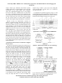
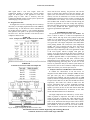
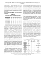
ISSN 2319-8885
Vol.02,Issue.13,
October-2013,
Pages:1487-1498
www.semargroups.org,
www.ijsetr.com
An On-Chip AMBA AHB Bus Tracer with Dynamic Compression and
Multiresolution for SOC Debugging and Monitoring
K.SWATHI1
N. DASHARATH2
PG Scholar, Dept of ECE, Netaji Institute of Engineering
and Technology, Hyderabad, A.P-INDIA,
Email: [email protected]
Asst Prof, Dept of ECE, Netaji Institute of Engineering and
Technology, Hyderabad, A.P-INDIA.
Abstract: This paper proposes an AMBA AHB on-chip bus
tracer named SYS-HMRBT (AHB Multiresolution bus
tracer) with dynamic compression and multiresolution for
Versatile System-On-Chip (SoC) debugging and monitoring.
The ON-CHIP bus is an important system-on-chip (SoC)
infrastructure that connects major hardware components.
Monitoring the on-chip bus signals is crucial to the SoC
debugging and performance analysis/ optimization. The bus
tracer is capable of capturing the bus trace with different
resolutions, all with efficient built-in compression
mechanisms, to meet a wide range of needs The bus tracer
adopts three trace compression mechanisms to achieve high
trace compression ratio, so that appropriate resolution
levels can be applied to different segments of the trace. On
the other hand, SYS-HMRBT supports tracing after/before
an event triggering, named post-triggering trace/pretriggering trace, respectively. SYS-HMRBT runs at 500
MHz and costs 42 K gates in TSMC 0.13-m technology,
indicating that it is capable of real time tracing and is very
small in modern SoCs. Experiments show that the bus tracer
achieves very good compression ratios of 79%–96%,
depending on the selected resolution mode. The SoC has
been successfully verified both in field-programmable gate
array and a test chip.
Keywords: AHB, AMBA, Compression, Multiresolution,
Periodical Triggering, Post-T Trace, Pre-T Trace, Real
Time Trace, System-On-Chip (Soc) Debugging.
I. INTRODUCTION
The On-Chip bus is an important system-on-chip (SoC)
infrastructure that connects major hardware components.
The on-chip bus signals monitoring is very important for
the SoC debugging and performance analysis/ optimization.
But to monitor such signals is very difficult since they are
deeply embedded in a SoC. T here are often no sufficient
I/O pins to access these signals. Therefore, we employ a
bus tracer embed in SoC to capture the bus signal trace and
store the trace in the trace memory which is an on-chip
storage, which could then be off loaded to outside world
(the trace analyzer software) for analysis. Unfortunately, the
size of the bus trace grows rapidly. For ex- ample, to capture
AMBA AHB 2.0 [1] bus signals running at 200 MHz, the
trace grows at 2 to 3 GB/s. Therefore, it is highly desirable to
compress the trace on the fly in order to reduce the trace
size. However, simply capturing/compressing bus signals is
not sufficient for SoC debugging and analysis. Since the debugging/analysis needs are versatile: some designers need
all signals at cycle-level, while some others only care about
the transactions. For the latter case, tracing all signals at
cycle-level wastes a lot of trace memory. Thus, there must be
a way to capture traces at different abstraction levels based
on the specific debugging/analysis need.
This paper presents a real-time multi-resolution AHB
on-chip bus tracer, named SYS-HMRBT (aHb multiresolution bus tracer). The bus tracer adopts three trace
compression mechanisms to achieve high trace
compression ratio. It supports multi-resolution tracing by
capturing traces at different timing and signal abstraction
levels. In addition, it provides the dynamic mode change
feature to allow users to switch the resolution on-the-fly for
different portions of the trace to match specific
debugging/analysis needs. Given a trace memory of fixed
size, the user can trade off between the granularities and
trace length to make the most use of the trace memory. In
addition, the bus tracer is capable of tracing signals before/
after the event triggering, named pre-T/post-T tracing,
respectively. This feature provides a more flexible tracing
to focus on the interesting points. The rest of this paper is
organized as follows. Section II surveys the related work.
Section III discusses the features in trace granularity and
trace direction. SectionIV presents the hardware architecture
of our bus tracer. SectionV provides experiments to
analyze the compression ratio, trace depth, and cost of our
bus tracer. A case study is also conducted to integrate the
bus tracer with a 3-D graphics SoC. Finally, Section VI
concludes this paper and gives directions for future
research.
Copyright @ 2013 SEMAR GROUPS TECHNICAL SOCIETY. All rights reserved.
K.SWATHI, N. DASHARATH
II. RELATED WORK
Since the huge trace size limits the trace depth in a
trace memory, there are hardware approaches to compress
the traces. The approaches can be divided into lossy and
lossless trace compression. The lossy trace compression
approach achieves high compression ratio by sacrificing
the accuracy; the original signals cannot be reconstructed
from the trace. The purpose of this approach is to identify
if a problem occurs. Anis and Nicolici [2] use the
multiple input signature register (MISR) to perform lossy
compression. The results are stored in a trace memory and
compared with the golden patterns to locate the range of
the erroneous signals. The locating needs rerunning the
system several times with finer and finer resolution until
the size of the search range can fit in the trace memory.
Such approach is suitable for deterministic and repeatable
system behaviors. However, for a complex SoC with
multiple independent IPs, the on-chip bus activities are
usually not deterministic and repeat- able. Therefore,
lossless compression approaches are more appropriate for
real-time on-chip bus tracing. Existing on-chip bus tracers
mostly adopt lossless compression approaches. ARM
provides the AMBA AHB trace macro- cell (HTM) [3] that
is capable of tracing AHB bus signals, including the
instruction address, data address, and control signals. The
instruction address and control signals are compressed with
a slice compression approach (to be explained shortly). On
the other hand, the data address is recorded by simply
removing the leading zeros. The HTM supports a limited
level of trace abstraction by removing bus signals that are in
IDLE or BUSY state.
The AMBA navigator [4] traces all AHB bus signals
without compression. In the bus transfer mode, it also has a
limited level of trace abstraction by removing bus signals
which are in IDLE, BUSY, or non-ready state. The
AHBTRACE in GRLIB IP library [5] captures the AMBA
AHB signals in the uncompressed form. In addition, it does
not have trace abstraction ability. There are many research
works related to the bus signal compression. We
characterize the bus signals into three categories: program
address, data address/data and control signals. We then
review appropriate compression techniques for each
category. For program addresses, since they are mostly
sequential, a straight forward way is to discard the
continuous instruction ad- dresses and retain only the
discontinuous ones, so called branch/ target filtering. This
approach has been used in some commercial tracers, such
as the TC1775 trace module in TriCore [6] and ARM’s
Embedded Trace Macrocell (ETM)[7]. The hard- ware
overhead of these works is usually small since the filtering
mechanism is simple to be implemented in hardware. The
effectiveness of these techniques, however, is mainly
limited by the average basic block size, which is roughly
around four or five instructions per basic block [7], [8].
Other technique such as the slice compression approach [3]
targets at the spatial locality of the program address.
This approach partitions a binary data into several slices
and then records all the slices of the first data and then only
part of the slices of the succeeding data that are different
from the corresponding slices of the previous one (usually the
lower bit positions of the data). For data address/value, the
most popular method is the differential approach which
records the difference between consecutive data. Since the
difference usually could be represented with less number of
bits than the original value, the information size is reduced.
Hopkins and Mc- Donald–Maier showed that the differential
method can reduce the data address and the data value by
about 40% and 14%, respectively [9]. For control signals,
ARM HTM [3] encodes them with the slice compression
approach: the control signal is recorded only when the value
changes. As mentioned, compressing all signals at the
cycle-ac- curate-level does not always meet the debugging
needs. As SoCs become more complex, the transactionlevel debugging becomes increasingly important, since it
helps designers focus on the functional behaviors, instead of
interpreting complex signals.
TABLE I
Timing Abstraction
Motivated by the related works, our bus tracer combines
abstraction and compression techniques in a more aggressive
way. The goal is to provide better compression quality and
multiple resolution traces to meet the complex SoC
debugging needs. For example, our bus tracer can provides
traces at cycle-level and transaction-level to support
versatile debugging needs. Be- sides, features such as the
dynamic mode change and bidirectional traces are also
introduced to enhance the debugging flexibility.
III. TRACE RESOLUTION AND TRACE DIRECTION
The multi resolution trace mode and the pre/post-T tracing
are two important features for effective SoC debugging and
monitoring. They are discussed in this section in terms of
trace granularity and trace direction.
A. Trace Multiresolution
This section first introduces the definitions of the
abstraction level. Then, it discusses the application for each
abstraction mode.
1. Timing and Signal Abstraction Definition
The abstraction level is in two dimensions: timing
abstraction and signal abstraction. At the timing dimension,
it has two abstraction levels, which are the cycle level and
transaction level, as shown in Table I. The cycle level
captures the signals at every cycle. The transaction level
International Journal of Scientific Engineering and Technology Research
Volume.02, IssueNo.13, October-2013, Pages:1487-1498
AnOn-Chip AMBA AHB Bus Tracer with Dynamic Compression and Multiresolution for SOC Debugging and
Monitoring
records the signals only when their value changes (event
triggering). For example, since the bus read/ write control
signals do not change during a successful transfer; the tracer
only records this signal at the first and last cycles of that
transfer. However, if the signal changes its value cycle-bycycle, the transaction-level trace is similar to the cycle-level
trace. At the signal dimension, first, we group the AHB bus
signals into four categories: program address, data
address/value, access control signals (ACS), and protocol
control signals (PCS). Then, we define three abstraction
levels for those signals. As shown in Table II, they are full
signal level, bus state level, and
TABLE II
Signal Abstraction
size of this mode is huge, the trace depth is the shortest
among the five modes. Fortunately, it is acceptable since
designers using the cycle-level mode trace only focus on a
short critical period.
At Mode FT, the tracer traces all signals only when their
values are changed. In other words, this mode traces the untimed data transaction on the bus. Comparing to Mode FC,
the timing granularity is abstracted. It is useful when
designers want to skim the behaviors of all signals instead of
looking at them cycle-by-cycle. Another benefit of this
mode is that the space can be saved without losing
meaningful information. Thus, the trace depth increases.
At Mode BC, the tracer uses the BSM, such as NORMAL,
IDLE, ERROR, and so on, to represent bus transfer
activities in cycle accurate level. Comparing to Mode FC,
although this mode still captures the signals cycle-by-cycle,
the signal granularity is abstracted. Thus, designers can
observe the bus hand- shaking states without analyzing the
detail signals. The benefit is that designers can still observe
bus states cycle-by-cycle to analyze the system
performance.
master operation level. The full signal level captures all bus
signals. The bus state level further abstracts the PCS by
encoding them as states according to the bus-state-machine
(BSM). The states represent the bus handshaking activities
within a bus transaction. The master state level further
abstracts the bus state level by only recording the transfer
activities of bus masters and ignoring the handshaking
activities within transactions. This level also ignores the
signals when the bus state is IDLE, WAIT, and BUSY.
Fig.1. Multiresolution traces modes.
Combining the abstraction levels in the timing dimension and
the signal dimension, we provide five modes in different
granularities, as Fig. 1 shows. They are Mode FC (full
signal, cycle level), Mode FT (full signal, transaction level),
Mode BC (bus state, cycle level), Mode BT (bus state,
transaction level), and Mode MT (master state, transaction
level). We will discuss the usage of each mode in the
following.
2. Applications of Abstraction Modes
At Mode FC, the tracer traces all bus signals cycle-by-cycle
so that designers can observe the most detailed bus activities.
This mode is very useful to diagnose the cause of error by
looking at the detail signals. However, since the traced data
At Mode BT, the tracer uses bus state to represent bus transfer
activities in transaction level. The traced data is abstracted
in both timing level and signal level; it is a combination of
Mode BC and Mode BT. In this mode, designers can easily
understand the bus transactions without analyzing the signals
at cycle level.
At Mode MT, the tracer only records the master behaviors,
such as read, write, or burst transfer. It is the highest
abstraction level. This feature is very suitable for
analyzing the masters’ transactions. The major difference
compared with Mode BT is that this mode does not record
the transfer handshaking activities and does not capture
signals when the bus state is IDLE, WAIT, and BUSY.
Thus, designers can focus on only the masters’ transactions.
Please note that there is no mode supporting master
operation trace at cycle level, since the intension of observing master behaviors is to realize the whole picture.
Tracing master behaviors at cycle level is meaningless and
can be re-placed with Mode BC.
Multiresolution trace has two advantages for efficient
SoC debugging. First, it provides the customized trace for
diverse debugging purposes. Depending on the debugging
purpose, de- signers can select a preferred abstraction level
to observe bus signal variation. For designers debugging at a
higher abstraction level, it saves a lot of time analyzing the
skeleton of system operations. The idea is to make the
hardware debugging process similar to the software
debugging process. Designers can use the higher abstraction
level trace to obtain the top view and then switch to the lower
abstraction level trace on-the-fly to check the detail signals.
International Journal of Scientific Engineering and Technology Research
Volume.02, IssueNo.13, October-2013, Pages:1487-1498
K.SWATHI, N. DASHARATH
It also helps establishing the time line of system
behaviors. After, designers switch to the Mode FC to focus
on every signal at cycle level for error diagnosis. Please
note although the trace size per cycle is huge in this mode,
it is usually not necessary to trace a long period. Finally,
after Mode FC, designers can switch to Mode BC to see
what operations are affected by this bug. Since the
behavior at every cycle is worth noticing, this mode
preserves the cycle-level trace. However, since designers
only care about the behaviors instead of all signals, this
mode abstracts the signal level and speeds up the
debugging process.
Fig.2. Debugging/ monitoring process with dynamic mode
change. The trace size varies with the trace modes. Mode
FC consumes the largest space. Mode MT consumes the
smallest space.
Second, the multiresolution tracing saves trace sizes. Since
higher-abstraction-level traces capture abstracted data, the
required space is smaller. Therefore, given a fixed-size trace
memory, the trace depth (cycle) in the higher abstraction
level is larger than the traces in the lower abstraction level.
3. Dynamic Mode Change
Our bus tracer also supports dynamic mode change
(DMC) feature. This feature allows designers to change
the trace mode dynamically in real-time. As Fig. 3 shows,
the trace mode changes seamlessly during execution.
Dynamic mode change has two benefits. One is that it
pro- vides customized traces according to the debugging
purpose. The other is that designers can make tradeoffs
between the trace granularity and the trace depth. Thus, the
trace memory utilization is more efficient. Fig. 3 shows
an example using dynamic mode change to diagnose a
suspected bug. At first, de- signers can use Mode MT to
have the top view so that they can skim the master
behaviors very quickly. Then, when the time is closed to
the suspected bug, they can switch to Mode BT. This
provides more information about all operations on the bus
and thus, designers can check the detail operations.
Fig.4. Illustration of periodical triggering concept.
The dynamic mode change is achieved by setting up the
event registers. The event registers define the start/stop time
of a trace and the trace mode. Thus, when the trigger
condition meets and a new trace begins, the new trace starts
in the trace mode specified in the event registers. Details are
discussed in Section IV. To provide better debugging
flexibility, the captured traces can be abstracted into higher
abstraction level traces by our trace analyzer software. For
example, the traces of mode FC can be abstracted into
traces of mode FT, mode BC, mode BT, and mode MT. The
traces of mode BC can be abstracted into traces of mode BT
and mode MT. This feature increases the debugging
flexibility since designers can understand the waveform
more quickly in higher abstraction level and narrow down
the debugging range in the lower-abstraction-level
waveform.
A. Trace Direction: Pre-T/Post-T Trace
Supporting both trace directions provides the flexible
debugging strategies. As Fig.3 shows, the post-T trace
captures signals after a triggering event, while the pre-T
trace captures signals before the triggering event. The post-T
trace is usually used to observe signals after a known event.
The pre-T trace is useful for diagnosing the causes of
unexpected errors by capturing the signals before the errors.
The mechanisms of the pre-T trace and the post-T trace are
different. The Post-T trace is simpler since the start time
and the stop time are known. It is activated when the
Fig.3. Pre-T trace and post-T trace with respect to a matched
target event is matched and is turned off when the trace
target event.
buffer is full. On the other hand, the stop time of the pre-T
International Journal of Scientific Engineering and Technology Research
Volume.02, IssueNo.13, October-2013, Pages:1487-1498
AnOn-Chip AMBA AHB Bus Tracer with Dynamic Compression and Multiresolution for SOC Debugging and
Monitoring
trace is unpredictable. The solution is to start tracing as soon
as system reset (or some other turning-on event). When the
trace buffer is full, the new trace data wrap around the trace
buffer, which means the oldest data are sacrificed for the
newest ones.
Wrapping around the trace buffer causes a problem when
the trace needs to be compressed. Typical lossless
compression algorithms work by storing some initial
(previous) states of the trace first and then calculate the
relationship between the current data and the previous states.
Since the size of the relationship is smaller than the data
size, e.g., the difference, it saves spaces. The initial state of
the trace, which is stored at the head of the
Fig5. Trace buffer and assistant header position table. (a) The
wrapping around does not occur. (b) The wrapping around
occurs: the first trace is overwritten by the 17th trace.
Fig.6. Event register.
first trace is damaged because the initial state is overwritten.
Then, the oldest header register is adjusted tent to the second
trace. If necessary, more header position registers can be
allocated to support more segments in larger buffer.
IV. BUS TRACER ARCHITECTURE
This section presents the architecture of our bus tracer.
We first provide an overview of the architecture for the post-T
trace. We then discuss the three major compression
methods in this architecture. Finally, we show the extension
of the post-T architecture to support the pre-T trace.
Post-T Tracer Architecture Overview:
Fig.7 is the bus tracer overview. It mainly contains four
parts: Event Generation Module, Abstraction Module,
Compression Modules, and Packing Module. The Event
Generation Module controls the start/stop time, the trace
mode, and the trace depth of traces. This information is sent
to the following modules. Based on the trace mode, the
Abstraction Module abstracts the signals in both timing
dimension and signal dimension. The abstracted data are
further compressed by the Compression Module to reduce
the data size. Finally, the compressed results are packed with
proper headers and written to the trace memory by the
Packing Module.
1. Event Generation Module:
The Event Generation Module decides the starting and
stopping of a trace and its trace mode. The module has
configurable event registers which specify the triggering
events on the bus and a corresponding matching circuit to
compare the bus activity with the events specified in the
event registers. Optionally, this module can also accept
events from external modules. For example, we can connect
an AHB bus protocol checker (HPChecker) [12] to the Event
Generation Module, as shown in Fig. 8, to capture the bus
protocol related trace. Fig. 6 is the format of an event
register. It contains four parameters: the trigger conditions,
the trace mode, the trace direction, and the trace depth. The
trigger conditions can be any combination of the address
value, the data value, and the control signal values. Each of
the value has a mask field for enabling partial match. For
each trigger condition, designers can assign a desired trace
mode, e.g., Mode FC, Mode FT, etc., which al- lows the
trace mode to be dynamically switched between events. The
trace direction determines the pre-T/post-T trace. The trace
depth field specifies the length of trace to be captured.
2. Abstraction Module:
The Abstraction Module monitors the AMBA bus and
selects/filters signals based on the abstraction mode. The
bus signals are classified into four groups as mentioned in
Section III-A1. Then, depending on the abstraction mode,
some signals are ignored, and some signals are reduced to
states. Finally, the results are forwarded to the
Compression Module for compression.
TABLE III
COMPRESSION PHASES FOR DIFFERENT
SIGNAL TYPES
management, and mode change control. For packet
management, since the compressed data length and type
are variable, every compressed data needs a header for
International Journal of Scientific Engineering and Technology Research
Volume.02, IssueNo.13, October-2013, Pages:1487-1498
K.SWATHI, N. DASHARATH
interpretation. There- fore, this step generates a proper
header and attaches it to each compressed datum. In this
paper, we call a compressed data with a header as a packet.
Since the header generation takes time, to avoid long cycle
time, the header generation is implemented in one pipeline
stage. For circular buffer management, it man- ages the
accesses to the trace memory. Since the size of a packet is
variable but the data width of the trace memory is fixed,
this module collects the trace data in a first-input, first-output
(FIFO) buffer and outputs them to the trace memory until the
data size in the FIFO buffer is equal/larger than the data
width. If the tracing stops and the data size in the FIFO
buffer is smaller than the data width, one additional cycle is
required to output the remaining data to the trace memory.
When the tracer is in the pre-T trace mode, this module also
maintains the header position table mentioned in Section IIIB-II. For mode change control, it manages the insertion of
the special packet (called mode-change packet) that
distinguishes the current mode from the previous mode. Details are discussed as follows.
Fig.7. Multiresolution bus tracer block diagram.
Dynamic mode change can be achieved by changing the mode
in the abstraction module. Designers can achieve this by
setting the desired trace mode in the event register. However,
since the header of each packet does not include the mode
information because of space reduction, the decompression
software cannot tell how to decompress the packets.
Therefore, there must be a mode-change packet that
indicates the trace mode, placing between two tracers
belonging to two different modes. The format
Fig.8. Concatenation of mode-change packet for abstraction
mode switch. Header 4’b0000 indicates it is a mode change
packet.
Fig.9. Program addresses compression flow and trace format.
International Journal of Scientific Engineering and Technology Research
Volume.02, IssueNo.13, October-2013, Pages:1487-1498
AnOn-Chip AMBA AHB Bus Tracer with Dynamic Compression and Multiresolution for SOC Debugging and
Monitoring
It is very important to insert this packet at the right time.
Since the tracer is divided into several pipeline stages, during
mode change, there are two trace data belonging to two
modes in the pipeline stages. The insertion of the modechange packet must waits until the trace data belonging to the
previous mode to be processed. It is achieved by the mode
change controller in the Packing Module. It accepts the mode
change signal from the Event Generation Module and
monitors the Abstraction Module and the Compression
Module. When the last-cycle datum of the previous mode is
processed and created as a packet, the mode- change packet
is inserted into the FIFO with that packet at the same cycle.
The reason of writing the two packets at the same time is to
avoid pipeline stall due to inserting the mode-change packet,
since the pipeline stall will prevent the bus tracer from
accepting new input data and cause discontinuous traces.
B. Compression Mechanism
Although the Abstraction Module can reduce the trace
size, the remaining trace volume is still very large. To reduce
the size, the data compression approaches are necessary. Since
the signal characteristics of the address value, the data value,
and the control signals are quite different, we propose different
compression approaches for them
1. Program Address Compression
We divide the program address compression into three
phases for the spatial locality and the temporal locality. Fig.9
shows the compression flow. There are three approaches:
branch/ target filter, dictionary-based compression, and
slicing.
3. Dictionary-Based Compression
To further reduce the size, we take the advantage of the
temporal locality. Temporal locality exists since the basic
blocks repeat frequently (loop structure), which implies the
branch and target addresses after Phase1 repeat frequently.
Therefore, we can use the dictionary-based compression.
The idea is to map the data to a table keeping frequently
appeared data, and record the table index instead of the
data to reduce size. Fig. 10 shows the hardware
architecture. The dictionary keeps the frequently appeared
branch/target addresses. To keep the hardware cost
reasonable, the proposed dictionary is implemented with
a CAM-based FIFO. When it is full, the new address will
replace the address at the first entry of FIFO. For each
input datum
, the comparator compares the datum with
the data in the dictionary (table []). If the datum is not in
the table (match= Miss), the datum (uncompressed-data) is
written into the table and also recorded in a trace.
Otherwise (match=Hit), the index (match-index) of the hit
table entry is recorded instead of the datum.
The hit index can be further compressed. As we know, a
basic block is composed by a target address and a branch
address, and the branch instruction address appears right
after target instruction address. By the fact that basic blocks
repeat frequently, if the target addresses is hit at the table
entry i, the branch address will hit at the table entry
,
since these entries are stored in the dictionary in a FIFO way.
Therefore, instead of recording the hit index of that branch
address, we create a special header, called the continuous
hit, to represent that branch address if it meets this
condition. This is the packet format 1 in Fig. 9.
4. Slicing
The miss address can also be compressed with the
Slicing approach. Because of the spatial locality, the basic
blocks are often near each other, which mean the highorder bits of branch/target addresses nearly have no
change. Therefore, the concept of the Slicing is to reduce
the data size by recording only the different digits of
two
Fig.10. Block diagram of the dictionary-based compression
circuit.
2. Branch/Target Filtering
This technique aims at the spatial locality of the program
address. Spatial locality exists since the program addresses
are sequential mostly. Software programs (in assembly
level) are composed by a number of basic blocks and the
instructions in each basic block are sequential. Because of
these characteristics, Branch/target filtering can records
only the first instruction’s address (Target) and the last
instruction’s address (Branch) of a basic block. The rest
of the instructions are filtered since they are sequential and
predictable.
Fig.11. Block diagram of the slicing circuit.
consecutive miss addresses. To implement this concept in
hardware, the address is partitioned into several slices of
an equal size. The comparison between two consecutive
miss addresses is at the slice level. For example, there are
three address sequences: A(0001_0010_0000), B(0001_001
0_0110), C(0001_0110_0110). At first, we record
instruction A’s full address. Next, since the upper two
International Journal of Scientific Engineering and Technology Research
Volume.02, IssueNo.13, October-2013, Pages:1487-1498
K.SWATHI, N. DASHARATH
slices of address B are the same as that of the address A,
only the least-significant slice is recorded. For address C,
since the most significant slice is the same to that of the
address B, only the lower two slices are recorded. Fig. 11
shows the hardware architecture. It has the register REG
storing the previous data (
).The slice comparator
compares the slices of the current datum (
) and the
previous datum and produces the identical slice number
(
). This in- formation is forwarded to the packing
module to generate the proper header. This is the packet
format 3 in Fig. 9.
Table IV shows an example of the compression
approaches in Phases 2 and 3. At time 1, since the address
(0x00008020) cannot be found in the dictionary, it is
inserted into the dictionary entry 0 and is recorded in a
trace. At time 2, the address (0x00008030) is also a miss
address and inserted into dictionary entry 1. However, after
slicing, since only the lower two slices are different, only
the address 0x30 is recorded. At time5, because the address
(0x00008020) has been stored in the dictionary entry 0 at
time 1, only the index 0x0000 is recorded. At time 6, since
the address (0x00008030) also has been stored in the
dictionary entry 1, and its index is the previous address plus
1, we do not have to record anything except the header (as
the packet format 1 in Fig. 9), which indicates this is a hit
address and this meets the continue index condition.
5. Data Address/Value Compression
Data address and data value tends to be irregular and
random. Therefore, there is no effective compression
approach for data address/ value. Considering using
minimal hardware resources to achieve a good compression
ratio, we use a differential approach based on the subtraction. Fig. 12 shows the
bit of the difference value. The differential module
calculates the absolute difference value
. Since the
absolute difference between two data value may
TABLE IV
Example of Dictionary-Based Compression with Slicing.
Third, Fourth, And Fifth Columns Are Packet Headers.
Referring To The Three Types Of Packet Format In Fig.
10, Compressed Packets Are In Packet Format 3.
Compressed Packets 5 a n d 9 A re In Packet Format 2.
Compressed Packet and Are in Packet Format2
be small, we can neglect the leading zeros and use fewer
digits to record it. Therefore, the size of module calculates
the nonzero digit number
of the difference. Finally,
the encoded datum is sent to the packing module along
with
.
Fig.13. Data address/value trace compression format means
the sign magnitude.
Fig.12. Block diagram of differential compression circuit
for data address/value compression.
For simple hardware implementation, the digit number of
an absolute difference is limited to four types, as Fig. 14
shows. The header indicates the data trace format. If the
difference is larger than 65535 (216-1), the bus tracer
records the uncompressed full 32-bit data value. Otherwise,
the bus tracer uses 4-, 8-, or 16-bit length to record the
absolute differences, whichever is appropriate.
6. Control Signal Compression
We classify the AHB control signals into two groups:
access control signals (ACS) and protocol control signals
(PCS). ACS is signals about the data access aspect, such as
read/write, transfer size, and burst operations. PCS are
signals controlling the transfer behavior, such as master
International Journal of Scientific Engineering and Technology Research
Volume.02, IssueNo.13, October-2013, Pages:1487-1498
hardware compressor. The register REG saves the current
datum
and outputs the previous datum
. By
comparing the current datum with the previous data value,
the three modules comp, differential, and size of output
the encoded results. The comp module computes the sign
AnOn-Chip AMBA AHB Bus Tracer with Dynamic Compression and Multiresolution for SOC Debugging and
Monitoring
request, transfer type, arbitration, and transfer response.
Control signals have two characteristics. First, the same
combinations of the control signals repeat frequently,
while other combinations happen rarely or never happen.
The reason is that many combinations do not make sense
in a SoC. It depends on the processor architecture, the
cache architecture, and the memory type. Therefore, the IPs
in a SoC tends to have only a few types of transfer despite
the bus protocol allows for many transfer behaviors.
Second, control signals change infrequently in a transaction.
Because of these two characteristics, ACS/PCS are
suitable for dictionary-based compression. The idea is to
treat the signals in ACS/PCS as one group. Since the
variations of transfer types are not much and transfer types
repeat frequently, we can map them to the dictionary with
frequently transfer types to re- duce size. For example, the
original size of ACS is 15 bits. If we use 3-bit to encode the
signal combinations of ACS, we can re- duce trace size
by
. To simplify the hardware design for
cost consideration, this dictionary is also implemented as a
FIFO buffer. With this approach, the dictionary adapts itself
when the ACS/PCS behaviors change. Please notice that, in
full-signal level trace, both ACS and PCS are compressed
by the dictionary-based compression without abstraction. In
bus-state level trace, the PCS are first abstracted into states
by the BSM model and then compressed by the dictionarybased compression.
A. Extension of the Post-T Trace Architecture to Support
the Pre-T Trace
The bus tracer described in Sections IV-A and IV-B is for
the post-T trace. We now extend the bus tracer to support the
pre-T trace with the technique of periodical triggering. The
concept of periodical triggering is to break the relation- ship
between the new trace and the previous trace. This can be
achieved by resetting the internal data structure for data encoding. For example, the register REG keeping the previous
data in the slicing (see Fig. 11) and the differential
compressor (see Fig. 12) must be reset. Also, the table in the
dictionary-based compression (see Fig. 11) is the same. We
use Fig. 14 to illustrate the concept. It is an example
showing the periodical triggering of the differential
compression. The encoded result (the difference
) is
produced by subtracting the previous data |
from the
current data . For example, the encoded data is 2-5 3 at
time T. If the trace mode does not change, the current data
is registered for encoding the new data at the next cycle.
Otherwise, the flush signal asserts. Then, the register
keeping the previous data is reset and a new trace begins.
For example, at time T+2,
(11) is recorded in the
uncompressed format by subtracting 0 from it, which serves
as an initial state for the new trace. Please notice that no data
is lost during the reset, though the data storage cannot
accept new input data while it is reset. For example, the
register in Fig. 15 takes 1 cycle (T+2) to reset, during that
cycle, the input data (
with value 11) is recorded in
uncompressed format.
To implement the periodical triggering concept, we add
extension hardware to the original tracer, as shown in Fig. 15.
The Triggering Module decides the time to start a new trace
based on the trace length (a segment size). It asserts the
Fig.14. Example of periodical triggering in differential
compression
TABLE V
Specification of the Implemented Sys-HMRBT Bus
Tracer
TABLE VI
Syntheses Results under TSMC 0.13- µ m Technology
Fig.15. Extension architecture for supporting post-T trace.
Below is the ex- tension to the original bus tracer.
International Journal of Scientific Engineering and Technology Research
Volume.02, IssueNo.13, October-2013, Pages:1487-1498
K.SWATHI, N. DASHARATH
flush signal when a new trace begins. Since the
compression module is divided into several pipeline
stages, the flush signal is also pipelined to reset each
pipeline stage in order. This is necessary since the
Compression Module requires several cycles to process the
data belonging to the previous trace.
D. Integration into SoC
To integrate the bus tracer (including the trace memory)
into a SoC, we can simply tap the bus tracer to the AHB bus,
as shown in Fig. 16. The bus tracer can be controlled with
an on-chip processor (option 1) or an external debugging
host (option 2). For option 1, the processor configures the
bus tracer via a bus slave interface. After the bus tracer
compresses and stores the
TABLE VII
Trace Compression Ratio at Different Trace Modes
TABLE VIII
Tradeoffs between Trace Mode and Output Pin
traces into the trace memory, the processor can read the
traces via the bus slave interface of the trace memory. For
option 2, the slave interfaces of the bus tracer and the trace
memory can also be connected to a test bus. The external
debugging host can then access the test bus to control the bus
tracer and the trace memory via a test access mechanism,
such as IEEE 1500. In order to achieve real time tracing, the
bus tracer is pipelined to meet the on-chip bus frequency.
Since the trace data processing is stream-based, the bus tracer
can be easily divided into more pipeline stages to meet
aggressive performance requirements.
V. EXPERIMENTAL RESULTS
The specification of the implemented SYS-HMRBT bus
tracer is shown in Table V. It has been implemented at
C, RTL, FPGA, and chip levels. The synthesis result with
TSMC 0.13-µm technology is shown in Table VI. The bus
tracer costs only about 41 K gates, which is relatively small
in a typical SoC. The largest component is the FIFO buffer
in the packing module. The second one is the compression
module. The cost to support both the pre-T and post-T
capabilities (periodical triggering module) is only 1032
gates. The major component of the event generation module
is the event register, which is roughly 1500 gates per
register. As for the circuit speed, the bus tracer is capable of
running at 500 MHz, which is sufficient for most SoC’s with
a synthesis approach under 0.13-µm technology. If a faster
clock speed is necessary, our bus tracer could be easily
partitioned into more pipeline stages due to its streamlined
compression/packing processing flow. In the rest of this
section, we present the analysis of various system metrics of
the bus tracer, such as trace resolution, compression quality,
depth, trace memory size, and I/O pin count, etc.
A. Analysis of the Trace and Hardware Characteristics
To evaluate the effectiveness of our bus tracer, we
integrated it with ARM’s EASY (Example AMBA SYstem)
SoC plat- form [14]. Five C benchmark programs were
executed on this platform. The first 10 000 cycles of AHB
signals (a mixture of setup and loop operations) were captured
as a post-T trace under FC, FT, BC, BT, and MT trace modes,
respectively. The results were shown in Table VII. The
average compression ratios of these benchmark programs
range from 79% for the most de- tailed mode FC (full
signals, cycle-level) to 96% for the most abstract mode MT
(master state, transaction-level). In between are the other
modes with intermediate levels of abstraction.
Fig.16. Example of integrating the bus tracer into a SoC.
The high compression ratio achieved by our bus tracer
makes it possible to output the trace data to the outside
world in real time via output pins. Table VIII shows the
required minimal pin count for each trace mode, ranging
from 7 to 21. Please note that the pin counts can be shared
among different modes. For example, if there is 21 output
pins available for the bus tracer, all five modes could be
output in real time, whereas three modes (BC, BT, and MT)
International Journal of Scientific Engineering and Technology Research
Volume.02, IssueNo.13, October-2013, Pages:1487-1498
AnOn-Chip AMBA AHB Bus Tracer with Dynamic Compression and Multiresolution for SOC Debugging and
Monitoring
could be output in real time when there are 13 pins
available. However, with only seven pins, the bus tracer
could still output the trace at mode MT in real time.
Therefore, our bus tracer allows designers to customize the
pin resource and trace resolution for real time trace dumping
to match a diverse range of debugging needs. If output pins
are not available; we can also store the trace data in an on-chip
trace memory.
Yang Et Al.: On-Chip AHB Bus Tracer with Real-Time
Compression
TABLE IX
Trace Depth Analysis of Dynamic Mode Change
(DMC) In a 2 Kb Trace Memory
We further explored the dynamic mode change (DMC)
feature of our bus tracer. Table IX estimates the number of
cycles that can be captured in each trace mode under four
configurations of dynamic mode change in a 2 kb trace
memory (base on the information in Table IX). For each
configuration, the numbers in parenthesis show the size
percentage of the five modes in the trace memory
respectively. For example, configuration I captures trace
segments under modes FC, FT, BC, BT, and MT, with each
mode taking up 10%, 15%, 20%, 25%, and 30% of the trace
memory respectively. The resulted depth of each segment is
82, 144, 261, 398, and 736 cycles, respectively. This
experiment demonstrates that our bus tracer allows users to
dynamically zoom in/out the observation of the bus for
different level of details and for different periods of time, and
thus it is capable of supporting versatile SoC
development/debugging needs, such as module development,
chip integration, hardware/software integration and
debugging,
system
behavior
monitoring,
system
performance/power analysis and optimization, etc. Table XI
compares the features of our tracer with related AHB bus
tracers: ARM’s HTM [3], FS2 AMBA Navigator [4] and
LEON3 AHBTRACE [5]. (Since the TC1775 trace module
in TriCore [6] and ARM ETM [7], reviewed in Section II,
are for processor tracing instead of bus tracing, we do not
compare our work with them in the experiment).
not supported by HTM. Compared with HTM, our tracer supports all four kinds of signals (Paddr, Daddr, Dvalue, and
Ctrl), all with more aggressive compression algorithms. On
the other hand, AMBA Navigator and AHBTRACE support
all four kinds of signals, but do not provide any compression
support. For the trace direction, AMBA Navigator and
AHBTRACE support only the post-T traces, while HTM
and our tracer sup- port both pre-T and post-T traces. As for
the multi-resolution support, HTM and AMBA Navigator
have limited abstraction capability in the timing dimension.
They filter signals when the bus state is in the IDLE or BUSY
cycles. On the other hand, our tracer supports abstraction in
both timing and signal dimensions, which provides more
versatile debugging/monitoring functionalities and better
trace compression ratio. In addition, our tracer allows
dynamic mode change, which is a unique feature among all
AHB bus tracers.
It is not an easy task to conduct quantitative comparison.
HTM and AMBA Navigator are commercial products
which we do not have access to, and there is no
information about their trace quality available in literature.
However, based on the qualitative comparison in Table XI,
we could reasonably conclude that our tracer supports both
more features and better compression quality. On the other
hand, the technical information that in order to have a fair
comparison, we assume the full buffer utilization for both
post-T traces and pre-T traces. For the 1 kb trace memory,
the compression ratio of pre-T traces is about 6.71%
inferior to that of post-T traces. However, the difference is
reduced as the trace memory size increases: only 3.75%
for 16 kb trace memory. Practically speaking, the difference
(from 3.75% to 6.71%) between the pre-T and post-T
traces is not significant in most debugging/monitoring
needs. Should such difference matters, the designer
should choose a larger trace memory as permitted by the
global cost budget to minimize such difference.
TABLE XI
Comparisons with Related Bus Tracers
Of the three related works, ARM’s HTM is the only one
which attends to compress traces. It uses the slicing
technique to reduce the trace size of the pro- gram address
(Paddr) and control signals (Ctrl). On the other hand, the
data address (Daddr) trace size is reduced by removing the
higher order zeros. However, the data value (Dvalue) trace is
International Journal of Scientific Engineering and Technology Research
Volume.02, IssueNo.13, October-2013, Pages:1487-1498
K.SWATHI, N. DASHARATH
TABLE XII
Trace Depth Comparison for Various Configurations
of Our Periodical Triggering Approach
Des., Autom. Test Eur. Conf., Apr. 16–20, 2007, pp. 1–6.
[3] ARM Ltd., San Jose, CA, “ARM. AMBA AHB
Trace Macrocell (HTM) technical reference manual ARM
DDI 0328D,” 2007.
[4] First Silicon Solutions (FS2) Inc., Sunnyvale, CA,
“AMBA navigator spec sheet,” 2005.
[5] J. Gaisler, E. Catovic, M. Isomaki, K. Glembo, and S.
Habinc, “GRLIB IP core user’s manual, gaisler research,”
2009.
TABLE XIII
Compression Ratio Comparison of Pre-T Traces and
Post-T Traces
[6] Infineon Technologies, Milipitas, CA, “TC1775 TriCore
users manual system units,” 2001.
[7] ARM Ltd., San Jose, CA, “Embedded trace macrocell
architecture specification,” 2006.
[8] E. Rotenberg, S. Bennett, and J. E. Smith, “A trace
cache micro architecture and evaluation,” IEEE Trans.
Comput., vol. 48, no. 1, pp.111–120, Feb. 1999.
VI. CONCLUSION
I have presented an on-chip bus tracer SYS-HMRBT for
the development, integration, debugging, monitoring, and
tuning of AHB-based SoC’s. It is attached to the on-chip
AHB bus and is capable of capturing and compressing in
real time the bus traces with five modes of resolution.
These modes could be dynamically switched while tracing.
The bus tracer also supports both directions of traces: pre-T
trace (trace before the triggering event) and post-T trace
(trace after the triggering event). With the aforementioned
features, SYS-HMRBT supports a diverse range of
design/de- bugging/monitoring activities, including module
development,
chip
integration,
hardware/software
integration and debugging, system behavior monitoring,
system performance/power anal- ysis and optimization, etc.
The users are allowed to tradeoff between trace
granularities and trace depth in order to make the most use
of the on-chip trace memory or I/O pins. SYS-HMRBT
costs only 42 K gates, making it an valuable and
economical investment in a typical SoC. It runs at 500 MHz
in TSMC 0.13m technology, which satisfies the
requirement of real-time tracing. Experiment results show
it achieves high compression ratio ranging from 79% to
96% depending on the trace mode. In the future, we would
extend this work to more advanced buses/connects such as
AXI or OCP.
VII. REFERENCES
[1] ARM Ltd., San Jose, CA, “AMBA Specification
(REV 2.0) ARM IHI0011A,” 1999.
[2] E. Anis and N. Nicolici, “Low cost debug architecture
using lossy compression for silicon debug,” in Proc. IEEE
[9] A. B. T. Hopkins and K. D. Mcdonald-Maier, “Debug
support strategy for systems-on-chips with multiple
processor cores,” IEEE Trans. Comput., vol. 55, no. 1, pp.
174–184, Feb. 2006.
[10] B. Tabara and K. Hashmi, “Transaction-level modeling
and debug of SoCs,” presented at the IP SoC Conf., France,
2004.
[11] B. Vermeulen, K. Goosen, R. van Steeden, and M.
Bennebroek, “Com- munication-centric SoC debug using
transactions,” in Proc. 12th IEEE Eur. Test Symp., May 20–
24, 2007, pp. 69–76.
[12] Y.-T. Lin, C.-C. Wang, and I.-J. Huang, “AMBA AHB
bus protocol checker with efficient debugging mechanism,”
in Proc. IEEE Int. Symp.Circuits Syst., Seattle, WA, May
18–21, 2008, pp. 928–931.
[13] Y.-T. Lin, W.-C. Shiue, and I.-J. Huang, “A multiresolution AHB bus tracer for read-time compression of
forward / backward traces in a circular buffer,” in Proc.
Des. Autom. Conf. (DAC), Jul. 2008, pp. 862–865.
[14] ARM Ltd., San Jose, CA, “Example AMBA system
user guide ARM DUI0092C,” 1999.
[15] R. -T Gu, T.-C Yeh, W.-S Hunag, T.-Y. Huang, C.-H
Tsai, C.-N Lee, M.-C Chiang, S.-F Hsiao, and I.-J.H YunNan Chang, “A low cost tile-based 3D graphics full pipeline
with real-time performance monitoring support for opengl
es in consumer electronics,” in Proc. ISCE, Jun.20–23,
2007, pp. 1–6.
International Journal of Scientific Engineering and Technology Research
Volume.02, IssueNo.13, October-2013, Pages:1487-1498