Download DBS Tailoring System

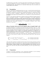
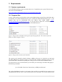
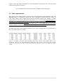
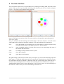
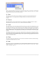
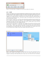
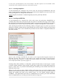
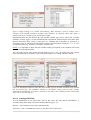
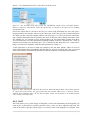
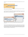
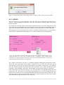
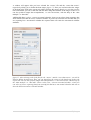
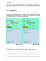
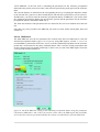
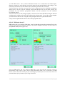
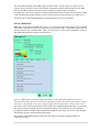
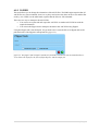
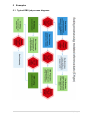
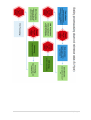
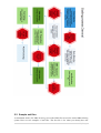
DBS Tailoring System
- a reference manual of the software
(version 1.0)
Kean Foster
Swedish Meteorological and Hydrological Institute
HI2.0_D342_DBS_Tailoring_System_a_reference_manual_(version_1) – Senast ändrad 2012-07-03
1
2|Page
Contents
CONTENTS........................................................................................................ 3
THE DISTRIBUTED BASED SCALING METHOD ............................................ 4
1
INTRODUCTION ................................................................................... 4
2
THEORY ................................................................................................ 4
2.1
The DBS Tailoring system ............................................................................... 4
2.2
Precipitation .................................................................................................... 5
2.3
Temperature ................................................................................................... 5
3
REQUIREMENTS .................................................................................. 7
3.1
System requirements ...................................................................................... 7
3.2
Program files ................................................................................................... 7
3.3
Data requirements........................................................................................... 8
4
THE USER INTERFACE ....................................................................... 9
4.1
Save.............................................................................................................. 10
4.2
Save to .......................................................................................................... 10
4.3
Load .............................................................................................................. 10
4.4
Clear ............................................................................................................. 10
4.5
Add ............................................................................................................... 10
4.5.1
4.5.2
4.5.3
4.5.4
4.5.5
LOAD
11
PLOT
14
EXPORT 16
DBS
18
FLIPPER 22
5
EXAMPLES ......................................................................................... 23
5.1
Typical DBS job process diagrams ................................................................ 23
5.2
Sample xml files ............................................................................................ 25
Acknowledgements
The development of the DBS tailoring system was co-funded by the national research programs
CLEO (CLimate change and Environmental Objectives) of the Swedish Environmental Protection
Agency and HYDROIMPACTS2.0 (Hydrological climate change impact scenarios: developing the
tools for a new generation) by the Swedish Research Council Formas.
3|Page
The Distributed based scaling method
1 Introduction
Today there is a huge demand for knowledge on climate change and the impact on our
environment. One source of information on possible outcomes of climate change is the numerical
global circulation models (GCMs). The GCMs model the climate for the entire globe, from the past
into the future. Different assumptions on how the greenhouse gas emotions will evolve can thus be
tested within this framework. However, the scale of the information obtained from those models
are often to coarse for any impact study on a regional scale. To downscale the information from the
GCMs either statistical methods or regional climate models (RCM) are used. Both methods have
their advantages and disadvantages. The RCMs hold more physics and might give a better
representation of the geographical variation. The statistical methods on the other hand are more
straightforward and don’t require the same amount of computational time as the RCMs. To make
the regional information useful in hydrological impact studies the information has to be even
further downscaled and bias corrected. The DBS Tailoring System presented in this reference
manual is an interface to a statistical method to do this downscaling and bias correction of two
variables important for hydrological modelling, namely precipitation and temperature. DBS is an
acronym for Distribution Based Scaling; the method was developed at the Swedish Meteorological
and Hydrological Institute.
2 Theory
2.1 The DBS Tailoring system
The DBS tailoring system is a tool used primarily for facilitating bias correction/downscaling using
the DBS approach (see the theory sections Precipitation and Temperature below). The DBS
tailoring system is used both to prepare the different data and control files needed to perform a
DBS bias correction/downscaling and run the DBS motor.
A typical DBS job can be broken down into six general steps:
1) Calculate the statistical parameters related to the reference precipitation. This step requires
an ASCII file containing observed precipitation (or the desired analogous substitute) for a
chosen reference period.
2) Calculate the statistical parameters related to the simulated precipitation. This step requires
an ASCII file containing modelled precipitation for a chosen reference period, and the
parameters from step 1.
3) The scaling of the simulated precipitation. This step requires an ASCII file containing
modelled precipitation for the entire period of interest and the parameters from steps 1 and
2.
4) Calculate the statistical parameters related to the reference temperature. This step requires
an ASCII file containing observed temperature (or the desired analogous substitute) for a
chosen reference period and the reference precipitation data again.
5) Calculate the statistical parameters related to the simulated temperature. This step requires
an ASCII file containing simulated temperature for a chosen reference period and the
results from the scaling of the precipitation data.
6) The scaling of the simulated precipitation. This step requires an ASCII file containing
modelled temperature for the entire period of interest and the following files; the
parameters from steps 2, 4 and 5, and the results from the scaling of the precipitation data.
4|Page
The DBS tailoring system helps to create the required files for the different steps described above
and controls the DBS motor in each step. The DBS tailoring system uses XML files to define how
to perform these tasks. These XML files are constructed with the help of the user-interface (see
sections 4 and 5 for more details).
2.2
Precipitation
In the case of precipitation, the DBS approach uses two steps: (1) spurious drizzle generated by the
climate model is removed to obtain the correct percentage of wet days and (2) the remaining
precipitation is transformed to match the observed frequency distribution. To obtain the percentage
of wet days correctly, a threshold is identified for each sub-basin and season. Days with
precipitation amount larger than the threshold value were considered as wet days and all other days
as dry days.
There are various theoretical distributions available to describe the probability distribution function
(PDF) of precipitation intensities. A commonly used distribution is the gamma distribution,
because of its ability to represent the typically asymmetrical and positively skewed distribution of
daily precipitation intensities (Wilks 1995; Haylock et al. 2006; Yang et al. 2008). A single gamma
distribution was therefore considered as the first choice in the DBS method, but then expanded as
discussed below. The gamma distribution is a two-parameter distribution whose density
distribution is expressed as:
= /
exp− 1⁄ , > 0
Γ
where is the shape parameter, is the scale parameter and Γ is the gamma function. The
distribution parameters were estimated using maximum likelihood estimation (MLE). Daily
precipitation distributions are typically heavily skewed towards low-intensity values. As a result,
the distribution parameters will be dominated by the most frequently occurring values, but may not
be able to accurately describe the properties of extreme values. To capture the main properties of
normal precipitation as well as extremes, the precipitation distribution was divided into two
partitions separated by the 95th percentile. The resulting distribution is hereafter referred to as the
double gamma distribution. Two sets of parameters – , and , , – were estimated from
observations and the RCA3 output in the control period (1961–1990). These parameter sets were in
turn used to correct the RCA3 outputs for the entire projection period up to 2100 using the
equation:
= = !" , !" , , #$% , #$% &
!", , !", , , #$%, , #$%, &
' < 95+ℎ-./0.1+'2.3425.
' < 95+ℎ-./0.1+'2.3425.
where Obs denotes parameters estimated from observations and CTL denotes parameters estimated
from the RCA3 output in the control period. F represents the gamma probability distribution. The
DBS parameters for daily precipitation were optimized separately for each sub-basin to preserve
spatial variability of the RCA3 outputs. To take seasonal dependencies into account, they were also
optimized for each season: DJF (Dec–Feb), MAM (Mar–May), JJA (Jun–Aug) and SON (Sep–
Nov).
2.3
Temperature
Compared to precipitation, temperature is more symmetrically distributed. It can be accurately
described by a normal distribution with mean m and standard deviation s:
5|Page
= 1
6√29
;
< @
:
?
. √=>
The mean and standard deviation of daily temperature on a Julian day were smoothed over the
control period using a 15-day moving window. Considering dependence between precipitation and
temperature, temperature time series were described with distribution parameters conditioned by
the wet or dry state of the day. Fourier series were used to smooth the seasonal mean and standard
deviation of temperature for wet and dry days:
M
4H,CD/EFG
A+ CD/EFG & =
+ J[4L,CD/EFG cosRS+ ∗ + TL,CD/EFG sinRS+ ∗ ]
2
∗
LN
M
0H,CD/EFG
6+ CD/EFG & =
+ J[0L,CD/EFG cosRS+ ∗ + XL,CD/EFG sinRS+ ∗ ]
2
∗
LN
where 4H , 4L , TL , 0H , 0L and XL are the Fourier coefficients, t* is the day of the year; w equals
2p/n, where n is the time units per cycle and k stands for the nth harmonic used for describing the
annual cycle of adjusted daily temperature, TDBS. Theoretically, t*/2 + 1 harmonics are able to
represent a complete cycle. Five harmonics were used and found to be sufficient.
The DBS parameters for temperature were calculated for both observations and RCM-simulated
data series. They are denoted A !" , 6 !" , A#$% and 6#$% and are used to scale the daily
temperature:
Y = 6
!" , A !" , YZ#[ , 6#$% , A#$% &
6|Page
3 Requirements
3.1 System requirements
To run the DBS tailoring system you need to have Java 7 installed on your system. The necessary
files can be downloaded from:
http://www.oracle.com/technetwork/java/javase/downloads/index.html
3.2 Program files
Create a work folder on your hard drive and copy the DBS tailoring system files to this folder and a
lib subfolder. Your folder should look like figure 1 and the lib folder should look like figure 2. The
program files can be downloaded from this address from within SMHI, \\winfsproj\proj\klimathydrologi\DBS\program_files or you can send a request for a download link to
[email protected] if you do not have access to the SMHI network.
figure 1. Image of the work folder showing the required program files. The contents of the lib
folder are shown in figure 2 below.
figure 2. Image of the contents of the lib folder.
The system can be opened by double clicking on DBS.jar; however it is advised to use the batch
file (Run_DBS.bat) to open the system as it increases the available computing resources to the
system and relative information regarding the scaling job can be read in the command window.
If you do not have access to the batch file you can make your own using a text editor and typing in
the following command:
java -Xss2048k -Xms512m -Xmx1024m -jar DBS.jar tasklist.xml
The yellow highlighted text above is the name of the xml file you would like the system to load
automatically on start up. This is not necessary and can be left blank. You can also add the term
7|Page
“nogui” to the end of the command; this will automatically load and run the xml file entered
without opening the user interface:
java -Xss2048k -Xms512m -Xmx1024m -jar DBS.jar tasklist.xml nogui
3.3 Data requirements
This version of the DBS Tailoring system works with precipitation and temperature data. An
important note: it is important to choose the correct temperature variables from the scenario to
scale. Some models have variables that represent non-grid-averaged data, which is a better
representation of observations than grid-averaged data. So if you are using observation data as a
reference it is encouraged that you try to use a non-grid averaged variable such as ‘tasol’
(temperature near surface over open land) from the RCA model. On the other hand, if you are using
modelled data as a reference e.g. EraInterim data, then it is encouraged that you use a gridaveraged variable e.g. t2m (2m temperature) and tas (temperature near surface).
The DBS stage of the system requires ASCII files to be ‘time’ oriented, that is to say with time on
the x-axis and id on the y-axis (fig).
figure 3. A sample of typical ‘time’ orientated data (left) and the same sample data in ‘id’
orientation. The files are tab delaminated ASCII files and can be created using any suitable
software e.g. Excel if you need to create them manually from data sources not supported by this
system.
8|Page
4 The User Interface
The user interface allows users to create DBS jobs by building and editing XML files that run the
system. When you first open the DBS tailoring system interface you will see a blank workspace
(figure 4), if you have not loaded an existing xml file).
figure 4. The blank user interface (left). The action wheel can be opened by right clicking in the
work space (right).
Here you can build and edit tailoring jobs with the help of the action wheel, to access the action
wheel right-click anywhere on the empty workspace. The action wheel has five alternatives:
Save:
saves the xml file you are working on to you work folder. If you have not previously
saved the xml file before it will open the ‘Save To’ option instead.
Save To:
opens a standard window for saving files where you can enter/change the name of
the xml file and the location.
Load :
for loading existing xml files into the system.
Clear :
clears the workspace.
Add:
opens the new task window.
By right clicking on the tasks (not on the empty work space) you will see the following drop down
menu (figure 5). With this drop down menu you can delete or edit the task you clicked on, insert a
new task before the task you clicked on, delete the entire list, or delete large parts of the task list i.e.
all tasks before excluding this task or all tasks after including this task, with the last two options.
Another helpful feature are the arrows that appear if you move the cursor over the left margin of
the task boxes. These allow you to move that task up or down the list.
9|Page
figure 5. By right clicking on the tasks you will get this menu. Here you can delete or edit the task
you clicked on, insert a new task before the task you clicked on, delete the entire list, or delete
large parts of the task list with the last two options.
4.1 Save
This option saves the xml file you are working on. If you have not saved it for the first time a
standard windows ‘save’ popup window will appear where you can enter the file name and
location.
4.2 Save to
This option allows you to save the xml file you are working on to a different location or under a
different name. It is the same as the ‘save as’ option in many other programs.
4.3 Load
This option allows you to open existing xml files saved on your system. If you already have an xml
file open in the interface you will be asked if you want to add the xml file to the end of open group.
If you choose ‘yes’ the tasks in the xml file that you are loading will be added to those already in
the user interface to create one long group. If you choose ‘no’ the tasks in the xml file that you are
loading will be added as a new group after those already in the user interface to create two groups
of tasks.
The difference between one or more groups is that the tasks in each group are independent of those
in the other groups. This means that if a job crashes in a critical task in one group the system will
skip to the next group and continue running. If you only have one long group the entire job will
crash if a critical task crashes.
4.4 Clear
This option on the action wheel allows you to clear the user interface of all tasks, instead of having
to delete the individual tasks one at a time.
4.5 Add
This option on the action wheel allows you to add the different individual tasks and in that way
build up an xml file. The individual tasks used to build an xml file are; ‘load’, ‘plot’, ‘export’
‘DBS’, and ‘flipper’ (figure 6).
10 | P a g e
figure 6. New task window, for adding one of the five base tasks to the workspace.
4.5.1 LOAD
This base task allows you to load file information for different file types into the system. Left
clicking on the task in the workspace will open a tab where you can choose which file you want to
use in the system. At the moment the system can only work with three types of files (figure 7);
shapefiles (see Loading shapefiles), netCDF files (see Loading netCDF files) and three types of
ASCII data (see Loading ASCII files). The other file types are unavailable in this version but will
be activated in future versions.
This step creates a ‘posmap’ file; a file that contains information regarding the data contained in the
file i.e. number of data points, data ranges etc. These POSMAP files, with their information
regarding how the data is stored in each file, allows the system to identify where in the ASCII files
the is stored which allows for faster reading of the data.
If you have prior tasks that have created data files, clicking on the source box will give you the
option to load a ‘system file’ or a ‘task output’. By choosing ‘system file’ you will enter the menu
as seen in figure 7 below, while choosing ‘task output’ will open a drop down menu with all the
task outputs that can be loaded at that stage. Click on the green light to save settings and close the
tab. By clicking on the red light will cancel any changes made and close the tab.
figure 7. Left clicking on the task opens the task tab. Here you can choose the data you want to
load into the system by right clicking in the source box, the currently supported file types are
shapefiles, netCDF files and ASCII files (discrete data, time series with time as the X axis header,
11 | P a g e
or time series with ID number as the X axis header). The other options are not available in this
version but will be available in the next version of the system.
4.5.1.1 Loading shapefiles
To load information for a shapefile, click on the source box and choose SHAPEFILE. This will
open a normal windows load window where you can choose the shapefile you want to load. Click
on the green light to save settings and close the tab.
NOTE: shapefiles should have a latitude/longitude projection, preferably WGS84.
4.5.1.2 Loading netCDF files
To load information for a netCDF file, click on the source box and choose SHAPEFILE. A
secondary drop down menu will open but only one option is selectable at this stage. Choose single,
this will open a normal windows load window where you can choose the netCDF file you want to
load information for. NOTE: netCDF files should have a latitude and longitude as field variables.
After selecting the netCDF file the following window will appear (figure 8) where you need to
identify the netCDF variables that are needed. Right click on the relevant variables and select from
the menu to set the field. To use a netCDF file you need to set four fields i.e. longitude, latitude, the
data field, and time.
figure 8. After selecting a netCDF file you need to set the required fields longitude, latitude, the
data field, and time. This is done by right clicking on the variable and setting it to the appropriate
field. Selecting ‘Show attributes’ or ‘Show data’ options displays the netCDF variable attributes
and a sample of the data respectively (figure 9).
Selecting either ‘Show attributes’ or ‘Show data’ options from the menu, as seen in figure 8, opens
a window with the attributes of the netCDF variable and a sample of the variable data respectively
(figure 9). This can be very useful for determining the calendar type and variable units which are
important in later steps.
When you right click on ‘time’ another window will appear, here you will be asked to input
optional ‘time’ related information. Here it is possible to set the start date for the netCDF data and
change the calendar type used in the netCDF (figure 10). The default calendar setting is
‘NORMAL’. The option ONLY360 refers to a calendar that uses a 360 day year while NOLEAPS
refers to calendar that uses a 365 day year but does not have leap years.
12 | P a g e
figure 9. Right clicking on a variable and choosing ‘Show attributes’ opens a window with a
summary of the netCDF variable’s attributes (left). Similarly, by choosing ‘Show data’ opens a
window that shows a sample of the variable data (right).
Information about the start date for the data and the calendar type can be seen in the ‘Variable
attributes’ window (figure 10) and calculated from information found using the and ‘Show data’
function described above (figure 8 and figure 9). Although this information is optional it is
advisable to enter it, otherwise all data will have relative time step labels starting at 1 i.e. 1, 2, 3 etc.
as opposed to dates e.g. 19610101, 19610102, 19610103 etc.
NOTE: it is important to check that the calendar setting corresponds to the calendar used in the
netCDF to avoid temporal shifts.
You can only proceed when all the relevant fields are set i.e. the ‘ok’ button will only become
active when this step is complete. Click on the green light to save settings and close the tab.
figure 10. Information about the start date and calendar type for the data contained in the netCDF
can be entered here. The NORMAL calendar is the default setting with two other options,
ONLY360 and NOLEAPS. If no date is entered for the data in the netCDF file then relative time
steps will be used starting at 1.
4.5.1.3 Loading ASCII files
To load information for an ASCII file, click on the source box and choose ASCIIDATA. A
secondary drop down menu will open with three choices (figure 11):
Discrete – non continuous data such as parameter files.
Timeserie – ‘time’ orientated time series i.e. they have time on the x-axis.
13 | P a g e
Idserie – ‘id’ orientated time series i.e. they have id on the x-axis.
figure 11. The secondary drop down menu for ASCIIDATA contains three selectable options:
Discrete, Timeserie, and Idserie. Select the option that is relevant to the data you are loading
information from.
Choose the option that is relevant to the file you want to load information for, this will open a
normal windows load window where you can choose the ASCII file you want to load information
for. When you have done this another window will open (figure 12). Here you need to confirm the
type of ASCII information the file contains, data series or discrete values, and the orientation of the
file, whether it is ‘Id’ oriented or ‘time’ oriented (choose ‘Id’ for discrete data). Further down there
are two fields where you enter information regarding headings in the file. ‘Header at row:’ refers to
which row the header is on (normally this is row 1) and the second ‘Skip first rows:’ refers to how
many rows need to be skipped to reach the data (again this is usually 1).
At this point there is no need to make any changes to the last three options. These are used to
import information about geographical data that may be saved in an ASCII file. Here you would
enter which columns contain the id information, latitude information and longitude information.
figure 12. After selecting the ASCII file for which to load information about, this window appears
in which you need to select the type of data the file contains (data series or discrete values),
indicate the orientation (select ‘Id’ for discrete data), which row the header is on and how many
rows to skip to reach the data.
4.5.2 PLOT
This task allows you to create images of shapefiles. Load in the information for the shapefile you
want to plot, as described in Loading shapefiles above. Once you have added the plot task, left
click on the task to open the task tab (figure 13). Source refers to the shapefile to be plotted, click
14 | P a g e
in the source box, select task output and choose the shapefile from the dropdown menu as shown in
figure 13.
figure 13. The ”Plot” task tab, to choose the shapefile you wish to plot from navigate the dropdown
lists and click on the desired shapefile.
A popup menu will appear listing the different variables in the shapefile (figure 14), here you can
choose “<all items>” to create plots for all variables or choose a specific variable from the
dropdown menu to create a plot for just that variable.
figure 14. A popup with a dropdown menu with the different variables that can be chosen. Here
you can choose <all items> if you wish to plot all of them, otherwise chose the one you are
interested in.
Clicking on OK will automatically fill the “Data source” box with your choice. Next, click on the
“Target” box; here you enter the location and name of the images that will be created. It is advised
to save the images as PNG files; this is done by adding “.png” as the file extension when entering
the file name. When this is done a popup window will appear figure 15asking you to enter the
image width. The larger the number the larger the image so you are free to choose the image size; a
width of 800 is suggested for a standard sized image.
15 | P a g e
figure 15. Popup box to eneter in the image width, a width of “800” can be used as standard.
4.5.3 EXPORT
This task allows you to export data from a file. The task can be divided into two main types of
export i.e. using geographic information to select the relevant data, and using unique ids to select
the relevant data.
The former type is mostly used to extract data from netCDF files to be in the scaling process. The
export task uses the geographic data in the shapefile to select the nearest corresponding point in
space from the netCDF file and assigns the id number from the shapefile to the data at that point.
The latter type is more versatile and can be used for a number of different tasks e.g. export statistics
for the data to a shapefile for analysis purposes, or extract a subset from an existing dataset.
figure 16. The ’Export’ task tab. Here you can enter the shapefile and data source files
being used into the ‘source’ and ‘extra data source’ respectively. After clicking on the
target box you need to choose what type of file you are exporting the data to, at present
only shapefiles and ASCII files are supported.
The “Export” task requires two files, 1) a shapefile captaining information on the data to export,
and 2) the source data which can be either a netCDF file or an ASCII file (both time and id
orientated files work). In this version of the program it is possible to export data to two different
file types, namely shapefiles and ASCII files. The ASCII files can be further divided into three
subgroups; ‘time-orientated’ ASCII files, ‘ID-orientated’ ASCII files and ‘discrete’ ASCII files.
Click on the task to open the task tab (figure 16). The source data is the shapefile that will be used
in the export job, click in the box and navigate the dropdown list to select the shapefile that you
intend to use (you need to have loaded the information into the system prior using a load task). The
extra data source is the file from which the data will be exported (again you need to have loaded
the information into the system prior using a load task).
16 | P a g e
A window will appear after you have selected the “source” file and the “extra data source”
respectively asking you to define the data ranges (figure 17). Here you can limit/select the ranges
of the data being used in the export task either selecting the ranges directly or, as in the case for
time related data; you can set the start and end dates using these buttons in the ranges section. You
can also perform simple data manipulations, i.e. unit conversions, with the help of the “data
multiple” or “data add”.
Additionally there is a box, “convert to normal calendar”, that you can select when exporting data
from netCDF files that do not use a normal calendar. If you do not select this box and the data you
are exporting has a non-normal calendar the exported data will retain the non-normal calendar
attributes.
figure 17. After selecting each of the files for the “source” and the “extra data source” you will be
asked to define the data item. Here you can limit/select the ranges of the data being used in the
export task. You can also perform simple data manipulations, i.e. unit conversions, with the help of
the “data multiple” or “data add”. There is also a box, “convert to normal calendar”, which you
can select if you are exporting data from a netcdf file that has a non-normal calendar and wish to
have the data converted to a normal calendar.
17 | P a g e
4.5.4 DBS
This task prepares the ‘info_DBS_generator.txt’ file which controls the DBS engine ‘DBS_generator.exe’, which performs the scaling. To perform a scaling job you will need to set up
six different DBS tasks, three for each variable. The first two tasks prepare parameter files for the
observed and simulated datasets respectively and the third uses these parameter files to perform the
scaling.
4.5.4.1 DBS tasks 1 and 2
The first two DBS tasks calculate the parameters for the reference and simulated precipitation
dataset to be used in the scaling of the scenario data later. The DBS engine must be saved in a work
folder where all the necessary files for the scaling tasks are/will be saved. In figure 18, below, you
have the first two of the DBS tasks where the parameters for the reference precipitation and the
simulated datasets are calculated. You need to enter where the DBS engine and the work folder are
located (as mentioned above, these should be in the same folder).
figure 18. The first two DBS tasks, perparing the parameter files for the reference (observed) and
the simulated data sets. Here you need to enter where the DBS engine and work folder are located
and define the reference period. You can also change how the seasons are defined here.
The seasons are each three months as default, you can change the number and length of the seasons
by selecting the season number and then clicking on the month you want in that season.
You need to enter the period for this task. That is the date when the DBS engine needs to start
calculating and the end date. These dates are entered in a popup window with the following format
18 | P a g e
YYYY-MM-DD. As the first task is calculating the parameters for the reference precipitation
dataset the time period you need to enter is the reference period being used (period of the reference
data).
The relevant datasets are entered into the corresponding boxes by navigating the dropdown menus
to the relevant files (you have to have loaded this file info into the system before you can select it).
In DBS task 1 you need to enter the reference precipitation dataset, in DBS task 2 you need to enter
the simulated precipitation dataset (for the reference period) and the parameters for the reference
precipitation dataset (calculated in DBS task 1).
The name and location of the parameter files are entered in the save boxes furthest down the task
tab.
Note that every time you add a new DBS task you need to re-enter all the search paths, dates and
seasons etc.
4.5.4.2 DBS task 3
The third DBS task uses the two parameter files created in the first two DBS tasks to scale the
simulated precipitation dataset (figure 19). If you are using DBS engines versions 1, 2 or 3 it is
recommended to perform this task twice, once to scale the simulated precipitation for the reference
period and a second time for the entire simulated dataset. This is because scaled precipitation data
for the reference period is needed in DBS step 5 and it is not yet clear if the DBS engine selects the
correct period from the full data set.
figure 19. The third DBS task, scaling of the simulated precipitation dataset using the parameters
calculated in DBS tasks 1 and 2. Here you need to reenter where the DBS engine and work folder
are located, the reference period and redefine the seasons, if needed done in previous BDS tasks.
19 | P a g e
As with DBS tasks 1 and 2, all the information needs to be re-entered for the DBS engine,
directory, seasons etc. only this time you need to enter the start and end date for the scaling i.e. the
reference period for the first run and the entire simulation period for the second run.
You then need to select the necessary files for the scaling process; the simulated precipitation
dataset (first a file for only the reference period and then the file for the entire period), the
parameters for the reference precipitation dataset, and the parameters for the simulated
precipitation dataset.
You can choose to save the scaling strengths, a measure of how much the DBS scaling has affected
each data point, which can be useful for analysing the scaling results. To save the scaling strengths
you must click on the box for saving the scaling strengths and select a path and file name.
Lastly select the path and file name for the scaled precipitation data.
4.5.4.3 DBS tasks 4 and 5
DBS tasks 4 and 5 are similar to DBS tasks 1 and 2 in that they prepare the parameter files for the
reference and simulated temperature datasets. They differ, though, in that they use files related to
precipitation in the process (figure 20).
figure 20. DBS tasks 4 and 5 are similar to DBS tasks 1 and 2 only that they need files related to
precipitation in the process. Again, all the initial information needs to be re-entered as per DBS
tasks 1,2 and 3, then the relevant files for calculating the paramete files are entered as well as the
path and names of the parameter files being calculated.
20 | P a g e
The initial data (the path to the DBS engine and work folder, seasons, dates etc.) needs to be reentered. Then you need to enter in the reference temperature and precipitation datasets into DBS
task 4 so that the parameters for the reference temperature dataset can be calculated.
For DBS task 5 you need to enter the simulated temperature dataset and the results from the scaling
of the simulated precipitation dataset for the reference period (as discussed above in DBS task 3).
And again enter in the path and filenames for the parameter files to be calculated.
4.5.4.4 DBS task 6
DBS task 6 is the last of the DBS tasks (figure 21), scaling the temperature dataset. Once again the
initial data in the header needs to be entered as per the previous tasks, except that the period is now
just the period of the simulated data. There are more files to enter as the temperature scaling is
dependant information from the precipitation files.
figure 21. DBS task 6, scaling the temperature dataset. The initial information needs to be reentered in the header, the period is the entire simulation period. Then all the required files need to
entered. It is not possible to save the scaling strengths for the temperature scaling in this version.
You need to enter in the required files for the scaling; the simulated temperature data set, parameter
files for the simulated and the reference temperature datasets, the parameters for the simulated
precipitation dataset, and the scaled simulated precipitation data. Lastly you need to enter the path
and filename for the scaled simulated temperature.
This version of the DBS tailoring system does not support saving the scaling strengths for
temperature scaling.
21 | P a g e
4.5.5 FLIPPER
This task allows you to change the orientation of the ASCII files. The DBS engine requires that all
ASCII files are ‘time-orientated’, that is to say they need to have the dates on the x-axis and the IDs
on the y-axis. HYPE, on the other hand, requires that the files are ‘ID-orientated’.
There are two ways to transpose the ASCII files:
•
•
You can use an export task and export the ASCII file as another ASCII file but with the
required orientation.
You can use the flipper task to transpose the data in the ASCII file being flipped.
Using the flipper task is much simpler, all you need to do is enter the file to be flipped and set the
path and name of the flipped or transposed file (figure 22).
figure 22. The flipper task transposes ASCII files from ID-orientated to time-orientated and viceversa. Enter the input file, the file to fllip/transpose, and the output file.
22 | P a g e
5 Examples
5.1 Typical DBS job process diagrams
23 | P a g e
24 | P a g e
5.2 Sample xml files
As mentioned earlier (The DBS Tailoring system) the XML files are used to run the DBS tailoring
system. Here are two examples of xml files. The first file is for when you already have the
25 | P a g e
reference data in ASCII form and the second is for when you have to extract reference data from a
netCDF file i.e. when using EraInterim data.
Please note that these are examples and are not generic for every situation, you will need to at least
need to input your own data, filenames, dates etc.
tasklist_a.xml
tasklist_b.xml
26 | P a g e