Download SBC CyclePO4=3=Hach A4 Portrait User Manual - Sea

150817CyclePO4
Cycle phosphate (PO4) sensor
User manual
08/2015, Edition 6
Table of Contents
Section 1 Specifications .................................................................................................................... 3
1.1 Mechanical................................................................................................................................... 3
1.1.1 Bulkhead connectors........................................................................................................... 3
1.1.1.1 6-contact connector.................................................................................................... 3
1.1.1.2 8-contact connector.................................................................................................... 3
1.2 Electrical....................................................................................................................................... 3
1.3 Optical.......................................................................................................................................... 4
1.4 Analytical...................................................................................................................................... 4
Section 2 Operation ............................................................................................................................ 5
2.1 Sensor setup................................................................................................................................ 5
2.1.1 Assemble the sensor........................................................................................................... 5
2.1.2 Install the software.............................................................................................................. 8
2.1.3 Prime the sensor................................................................................................................. 9
2.1.3.1 Prepare to prime the sensor....................................................................................... 9
2.1.3.2 Prime sensor with vacuum....................................................................................... 11
2.1.3.3 Fill sensor filters....................................................................................................... 11
2.2 Prepare sensor for deployment.................................................................................................. 12
2.3 Deployment................................................................................................................................ 15
2.3.1 Modes of operation............................................................................................................15
2.3.2 Set up for deployment....................................................................................................... 15
2.3.2.1 SDI operation........................................................................................................... 16
2.3.2.2 SDI deployment........................................................................................................ 17
2.3.3 Deployment procedures.................................................................................................... 18
2.3.4 Complete the deployment................................................................................................. 18
2.4 Optional in-laboratory performance analysis ............................................................................. 19
2.4.1 Setup for in-laboratory performance analysis....................................................................19
2.4.2 In-laboratory sensor stability analysis............................................................................... 20
2.4.2.1 Use of water tanks for in-laboratory performance analysis...................................... 22
2.4.3 NIST check standards for in-laboratory performance analysis.......................................... 22
2.4.4 Solutions for in-laboratory performance analysis.............................................................. 22
2.5 Data analysis.............................................................................................................................. 22
2.5.1 Files tab............................................................................................................................. 22
2.5.2 Operation sequence.......................................................................................................... 24
2.5.3 Blank run example.............................................................................................................24
2.5.4 Good quality calibration data............................................................................................. 25
2.5.5 Bad data............................................................................................................................ 26
2.6 Data QA/QC............................................................................................................................... 26
2.6.1 Open data files for analysis............................................................................................... 26
2.6.2 Compare data files............................................................................................................ 27
Section 3 Maintenance ..................................................................................................................... 31
3.1 Clean and lubricate bulkhead connector.................................................................................... 31
3.2 Clean macro-fouling................................................................................................................... 31
3.3 Clean sensor flow paths with cleaning solution ......................................................................... 31
3.3.1 Clean flow paths with bleach solution............................................................................... 33
3.4 Flush cleaning solution from flow paths..................................................................................... 34
3.5 Replace reagent cartridges........................................................................................................ 34
3.6 Replace intake filter and screen................................................................................................. 35
3.7 Prime sensor with vacuum......................................................................................................... 35
3.8 Send reagent cartridges back to manufacturer.......................................................................... 36
3.9 Sensor storage........................................................................................................................... 37
3.9.1 Short-term storage............................................................................................................ 37
1
Table of Contents
3.9.2 Long-term storage............................................................................................................. 37
Section 4 Reference ..........................................................................................................................39
4.1 Description of nutrient units........................................................................................................ 39
4.2 Cycle commands........................................................................................................................ 39
4.2.1 Configuration commands.................................................................................................. 40
4.2.2 Operation commands........................................................................................................ 43
4.2.3 File commands.................................................................................................................. 45
4.2.4 Miscellaneous commands................................................................................................. 47
4.2.5 SDI commands.................................................................................................................. 49
4.3 Software reference..................................................................................................................... 56
4.3.1 Engineering units output....................................................................................................56
4.3.2 Raw transmittance output..................................................................................................57
4.3.3 Summary file format.......................................................................................................... 57
4.3.4 Raw file format.................................................................................................................. 57
4.3.5 File and tools menus......................................................................................................... 58
4.3.6 Communication setup........................................................................................................58
4.3.7 Operation values............................................................................................................... 59
4.3.8 Date and time setup.......................................................................................................... 59
4.3.9 Modes of operation............................................................................................................59
4.3.9.1 Operation options..................................................................................................... 60
4.3.9.2 Stop options............................................................................................................. 60
4.3.9.3 Low power option..................................................................................................... 60
4.3.10 Data file storage.............................................................................................................. 60
4.3.11 Status tab........................................................................................................................ 60
4.3.12 Plot tabs.......................................................................................................................... 61
4.3.12.1 PO4 plot tab........................................................................................................... 61
4.3.12.2 Raw data plot tab................................................................................................... 62
4.3.13 Settings tab..................................................................................................................... 63
4.3.13.1 Sample collection schedule.................................................................................... 63
4.3.13.2 Cycle deployment calculator.................................................................................. 64
4.3.13.3 Pump controls........................................................................................................ 64
4.3.13.4 SDI controls............................................................................................................ 64
4.3.14 Monitor tab...................................................................................................................... 65
4.3.15 Files tab........................................................................................................................... 65
4.3.16 QC Plot tab...................................................................................................................... 66
4.3.16.1 Cycle QC example................................................................................................. 67
Section 5 General information ....................................................................................................... 71
5.1 Warranty..................................................................................................................................... 71
5.2 Service and Support................................................................................................................... 71
5.3 Waste electrical and electronic equipment................................................................................. 71
2
Section 1
Specifications
1.1 Mechanical
Rated depth
200 m
Weight in air
6.8 kg (w/reagents)
Weight in water
0.37 kg
Height (w/handle)
56 cm
Diameter
18 cm
Temperature range, operation
0–35 °C
1.1.1 Bulkhead connectors
1.1.1.1
6-contact connector
Contact
Function
1
Ground
2
RS232 RX
3
External wake
4
Voltage in
5
RS232 TX
6
Analog 1
1.1.1.2
MCBH-6-MP
8-contact connector
Contact
Function
1
Voltage in
2
Ground
3
No connect
4
Bi-directional SDI-12
5
RS232 TX
6
RS232 RX
7
No connect
8
No connect
MCBH-8-MP
1.2 Electrical
Main port (6-pin)
SDI port (8-pin)
Input
10.5–18.0 V
Current draw, operation
115 mA avg, 2 A max
Current draw, low power
30 µA
Power dissipation
1.15 W avg, 12 W max
Communication interface
RS232 ASCII
SDI-12
Baud rate
9600–115,200
1200 baud
Data storage
1 GB compact flash card type II
125 mA avg, 2 A max (10 mA SDI-12)
3
Specifications
External "wake" high voltage
3.5–20.0 V
External "wake" low voltage
0.0–3.3 V
1.3 Optical
Wavelength
870 nm
Pathlength
5 cm
Linearity
> 95% R²
1.4 Analytical
Detection limit, three standard deviations of 18 MOhm water
less than or equal to 0.075 µM
less than or equal to 0.0023 mg/L PO4-P
Quantification limit, ten standard deviations of 18 MOhm
water
less than or equal to 0.025 µM
less than or equal to 0.0077 mg/L PO4-P
Range, nominal
0–10 µM
0–0.3 mg/L PO4-P
A higher range of 0–40 µM, 0–1.2 mg/L PO4-P is possible but outside specifications.
4
Section 2
Operation
2.1 Sensor setup
2.1.1 Assemble the sensor
CAUTION
Wear Personal Protective Equipment (PPE) to remove or replace cartridges. PPE includes a lab
coat or smock, gloves, safety glasses.
The Cycle PO4 sensor comes in two boxes. One is a fiberboard box with the reagent
cartridges. The second is a ruggedized plastic case with the sensor and spare parts.
1. Remove the sensor and the spare parts kit from the plastic case.
2. Remove the cartridges from the fiberboard box.
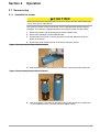
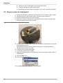
3. Set the sensor on its side to remove the seven screws that attach the protective
sleeve to the sensor.
4. Remove the seven Phillips screws on the sleeve. Keep the screws.
Figure 1 Screws removed from protective sleeve
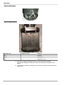
5. Hold the bottom of the sensor and bring it vertical to slide the protective sleeve off.
Figure 2 Sensor with protective sleeve removed
6. Look at the sensor. One side has the intake tubing to the sample port, marked with
"S," and calibration tubing. The other side has reagent tubing.
5
Operation
Figure 3 Intake tubing
Figure 4 Reagent tubing
Cartridge color
Location on sensor
Contents
Blue
S
phosphate
Yellow
R1
ascorbic acid
Red
R2
sulfuric acid, < 10%
7. Remove the reagent cartridges from the box and unwrap each cartridge.
Note that the cartridges are indexed so each one will only fit in one place on the
sensor.
8. Install the blue calibration cartridge first. Hold it above the upper housing, above the
intake ports.
6
Operation
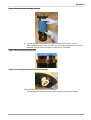
Figure 5 Blue calibration cartridge installed
9. Set the cartridge on the guide pins and push down until it "clicks" into place.
If the cartridge does not "click" into place, lift it off of the guide pins and push on the
stainless steel tab of the fluid coupler to make sure it is unlocked.
Figure 6 Blue cartridge on guide pins
Figure 7 Fluid coupler at the bottom of each cartridge
10. Install the yellow and then the red cartridge.
The cartridges are installed correctly if they cannot be lifted off of their bases.
7
Operation
Figure 8 Cartridges installed
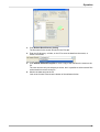
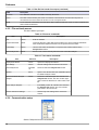
2.1.2 Install the software
Install the Cycle Host software from the Software tab on the Cycle Host product page on
the manufacturer's web site.
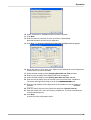
1. Make a Cycle folder in C:\Program Files(x86) on Windows Vista, Windows 7 or
Windows 8 or in C:\Program Files for earlier versions of Windows.
2. Make a CycleHost folder in the Cycle folder from the previous step.
3. Go to the downloaded zip file.
4. Right-click on the CycleHost.zip folder and choose Extract All...
5. Make sure that the "Show extracted files when complete" checkbox is selected.
6. Extract the files to C:\Program Files (x86)\CycleHost.
7. If asked for Administrator permission, push Continue.
The Cycle software files will "unzip."
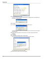
8. Go to the Cycle Host folder.
9. Double-click on the CycleHost.exe file.
8
Operation
10. If a Windows security warning shows, push Run to continue to install the Cycle Host
software.
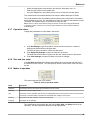
2.1.3 Prime the sensor
Note: Use a vacuum only to prime the sensor. Do not use pressure.
2.1.3.1
Prepare to prime the sensor
CAUTION
Wear Personal Protective Equipment (PPE) to remove or replace cartridges. PPE includes a lab
coat or smock, gloves, safety glasses.
The sensor comes with de-ionized (DI) water in all of the fluid passages. The user must
prime the sensor before it is turned on. This will move the reagents and calibration
standard into the fluid passages.
Table 1 Equipment needed to prime the Cycle
User-supplied
Manufacturer-supplied
2 receptacles for water
50 mL syringe
Regulated power supply
Test cable
PC
¼" outside diameter (OD) tubing, < 1 m in length
1. Find the ¼" OD Y-shaped tubing connected to the "S" mark on the sensor.
2. Pull the tubing from the hose barb next to the "S" straight off the barb. The barb is
angled up.
9
Operation
Figure 9 Y-shaped tubing disconnected from "S"
3.
4.
5.
6.
7.
Unwind the exhaust tubing from the top of the sensor.
Put one end of the exhaust tubing in an empty receptacle.
Fill another receptacle with 150 mL or more of DI water.
Connect the 50 mL syringe to the length of ¼" tubing.
Put the end of the tube in the de-ionized water and use the syringe to fill it with water.
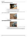
Figure 10 Tube filled with DI water
8. Make a kink in the tube near the syringe so that no water drains from the tube, and
remove the syringe.
Figure 11 Syringe removal from filled tube
9. Keep the tube with a kink in it and push it onto the hose barb near the "S" mark. Make
sure there is no air in the tubing or in the hose barb.
10. Connect the manufacturer-supplied test cable to the sensor, a power supply that can
provide 2 amps, and the host PC. The user will need a serial-to-USB adapter cable.
10
Operation
Figure 12 Sensor ready to be primed
11. Start the Cycle software if necessary.
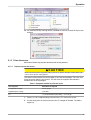
2.1.3.2
Prime sensor with vacuum
1. Attach the Luer-lock and the 1/16" ID barb adapter to the exhaust tubing and to the
supplied syringe.
2. Attach the syringe with the adapter to the outlet of the 1/16" ID sensor effluent tubing
that comes out of the top end flange.
3. Under the Settings tab, make a check in the "Cal" box and set the calibration pump to
operate for 100 pump cycles.
4. Push Run Pump(s).
5. While the pump is in operation, pull a light vacuum, approximately 1/5 (10 mL) of the
full travel of the plunger.
6. After the pump has operated for 100 cycles, make sure that the reagent tubing that
connects the cartridges and the inlet barbs does not have any air bubbles.
Look at the tubing from the reagent cartridges to the manifold to check for bubbles.
• If bubbles are present, do steps 4 and 5 again.
• If bubbles are small, it may not be possible to remove them.
7. Do steps 3–5 with R1 and R2.
8. Disconnect the tubing from the syringe.
9. Put the end of the tubing into an empty receptacle.
10. Go to the Settings tab and push Flush.
The Sample fluid opening is primed.
2.1.3.3
Fill sensor filters
1. Fill the filters with DI water:
1. Disconnect the 1/8" ID tubing that connects the filter to the "S" inlet barb if
necessary.
2. Connect the manufacturer-supplied syringe to the 1/8" ID tubing. Push clean
water into the filters.
3. Pinch the tubing and remove it from the syringe.
11
Operation
4. Connect it to the "S" barb again to prevent the loss of prime.
5. The filters will drip some water after this step.
It is not possible to remove all of the air bubbles. Try to remove as many as possible.
2.2 Prepare sensor for deployment
1.
2.
3.
4.
Use the host software to make sure that the sensor is in a low power ("sleep") mode.
Disconnect the test cable from the sensor, the power supply, and the PC.
Wind the exhaust tubing at the top of the sensor.
Make sure to align the indentations of the protective sleeve with the eye bolts, then
slide the protective sleeve over the sensor.
Figure 13 Protective sleeve aligned with eye bolts
5. Put the sensor on its side, hold the eye bolts, and align the screw holes for the sensor
and the protective sleeve.
Note that the protective sleeve is longer than the sensor. The screws cannot be
installed when the sensor is vertical.
6. Install the seven Phillips screws again.
7. If necessary, start the Cycle software.
8. Make sure that the sensor is connected to the host PC and a power supply, and is in
standby mode.
9. Go to the Tools menu.
10. Select the Deployment Wizard.
11. The Cycle Deployment Wizard window will appear.
12
Operation
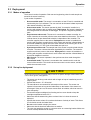
12. Select "Autonomous - Standalone with no external controller."
13. Push Next.
14. Enter the name of a directory in which to store the collected data.
Note that the name can have only 8 characters.
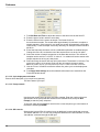
15. Push Next. The Priming and Sampling Start date and Time window appears.
16. Set up the sensor to do a prime cycle. Either use the Settings tab or the "Deployment
Wizard" before the sensor operates.
17. Select the date to deploy on the Sampling Start Date and Time calendar.
18. Enter the time to deploy at the Sample Start Time variable box.
19. Select the date to deploy on the Priming Start Date and Time calendar.
20. Enter the time to deploy minus 30 minutes in the Prime Start Time variable box.
The sensor will begin the priming cycle 30 minutes before it is deployed.
21. Enter the total samples for the deployment in the variable box next to Number of
Samples.
22. Enter the sample interval in the variable box area next to Sample Interval.
23. Keep the default of 6 in the Cal Frequency variable box. This is the manufacturer's
recommended frequency.
24. Push Next.
A summary of the configuration shows.
13
Operation
25. Push Send Settings to Cycle.
If the user selects a configuration that will have a negative effect on the operation of
the sensor, a window shows.
26. Push Yes.
27. Push Yes at the next window to make a configuration report.
Configuration values will still be sent to the sensor if the user does not want a report
and pushes No.
28. Enter a name and location to store the report. Use .txt or .log as the filename
extension.
29. Push Save.
30. Push Finish, then Yes to make a results report.
The results report records the new values and the previous values.
The sensor goes into a low power mode.
31. Disconnect the sensor from the power supply.
14
Operation
2.3 Deployment
2.3.1 Modes of operation
There are six modes of operation. Both raw and engineering units for each sample are
stored in the sensor's memory.
Cycle modes of operation:
•
•
•
•
•
•
Host-controlled mode. The sensor is connected to a host PC and is controlled and
monitored by the Cycle software. The user can look at the sensor's data output and
other status indicators in this mode.
Autonomous mode. The sensor operates by itself, for example, installed on a
mooring with a battery pack to supply power. Deployment: the sensor is installed on
a mooring that has no controller or data logger. The power is supplied by a battery
pack.
Asynchronous slave mode. The sensor is connected to a master controller. At
certain intervals, the controller pulls the most recent data from the sensor. The sensor
collects data on its pre-determined schedule, independent of the controller. The
controller supplies power to the sensor. Deployment: the sensor is installed on a
mooring with a system controller that is set to collect and send the collected data to a
shore-side database at regular intervals. Other sensors on the mooring turn on for
2 minutes of every 15. The Cycle collects data once per hour.
Synchronous slave mode. The sample rate of the sensor is synchronized with the
controller. The sensor collects data when signalled by the controller. The controller
supplies continuous power to the sensor. Deployment: the sensor is installed on a
mooring with a system controller that is set to collect and send the collected data to a
shore-side database in real-time.
SDI-12 mode. The sensor operates in the synchronous slave mode through the
SDI-12 port.
Commanded mode. The sensor is connected to the controller and is under the
control of the controller. This mode has the most control over the sensor, and also
needs the most work to use.
2.3.2 Set up for deployment
CAUTION
Wear Personal Protective Equipment (PPE) to remove or replace cartridges. PPE includes a lab
coat or smock, gloves, safety glasses.
•
•
•
•
•
•
•
•
•
The sensor can be hung under a dock with a length of rope or installed as part of a
larger system.
Operate the sensor ± 15° off-vertical.
The manufacturer recommends full submersion of the sensor. The sensor can
operate in less water as long as the intake filters on the bottom of the sensor are
submerged. If they are not, the sensor cannot flush air bubbles, which can result in
poor data quality.
Prevent the reagent cartridges from freezing and use a sun shade to keep the
cartridge temperatures below 35 °C.
Make sure that the waste tubing does not have kinks in it when the sensor is
deployed.
Operate the sensor at least 10 cm above the bottom of a body of water. This allows
for circulation around the intake filters.
Do not use the handle to deploy the sensor.
Make sure that the electrical cables have no tension.
The user may attach the sensor to a structure such as a mounting bracket. Make sure
to have a backup attachment for safety.
15
Operation
•
Use braided line rope, not twisted nylon, to support the cables.
Replace any questionable hardware that is less expensive than the data from the sensor.
Make sure screws, screw eyes, brackets, ropes, straps, zinc anodes, etc. are in good
condition. Replacement parts are available from the manufacturer or a marine supply
store.
The sensor effluent exits through the outlet tubing. Make sure the effluent flows freely and
does not go onto the sensor or its mounting. The effluent contains antimony and
molybdenum and has a pH of < 2. Make sure to wear the proper Personal Protective
Equipment (PPE) to work near this effluent. Refer to the MSDS that comes with the
reagent cartridges for specific information. Obey local, state, and federal laws to dispose
of waste. Contact the manufacturer for waste containment solutions.
2.3.2.1
SDI operation
All sensors that have an 8-pin connector can operate on an SDI-12 network.
SDI-12 version 1.3 is supported. Refer to the SDI-12 Version 1.3 specification at
http://www.sdi-12.org for details.
Required equipment
1. Cycle sensor with both 6- and 8-pin connectors
2. PC with Cycle host software installed
3. SDI recorder
16
Operation
4. Power supply
5. 6-socket test cable
6. 8-socket SDI cable.
Power requirements and sample setups
•
•
•
•
•
•
The sensor must have a minimum of 10.5 VDC at 2 amps.
The decrease in voltage over 30 m of 18-gauge cable is approximately 2.2 V.
Use a standalone power supply if the SDI recorder cannot supply 2 amps.
Connect the negative terminal of a standalone power supply to the ground terminal of
the recorder.
Do not connect the positive terminal of a standalone power supply to any terminal on
the recorder.
Make sure to add the power requirements of any SDI-capable sensor to the total
current requirement.
Sample setup 1
Equipment
Power requirement
sensor
Cycle PO4
10.5 VDC, 2 amps
cable length
60 m (200 ft)
4.4 VDC (200 x 2.2)
cable gauge
18
power supply
SDI recorder that supplies 12 VDC at 0.5 amps
14.9 VDC at 2 amps
Sample setup 2
Equipment
Power requirement
sensor
Cycle PO4
10.5 VDC, 2 amps
sensor
SUNA
12–18 VDC, 1 amp
cable length
30 m (100 ft)
3.3 VDC
cable gauge
18
power supply
SDI recorder that supplies 12 VDC at 0.5 amps
15.3 VDC at 3 amps
Note: Set the Cycle PO4 and SUNA to different SDI addresses. Change the Cycle from its default
of 0 to 1 before deployment.
2.3.2.2
SDI deployment
1. Connect the SDI cable to the 8-pin connector on the sensor.
2. Connect the other end of the SDI cable to the SDI recorder and a 12V power source.
Note that the power supply must supply a minimum of 2 amps.
3. Configure the SDI recorder to send "aM!" or "aC" commands at the chosen
frequency.
These will start measurements on a preset schedule.
•
•
•
The sensor will ignore the "aM!" and "aC" commands if a prime sequence is
scheduled but not complete. The sensor is primed before it starts to collect data.
The SDI schedules when to collect data. The sensor controls whether the data
measurement is spiked or normal.
Schedule the "aM!" or "aC" commands at an interval longer than 35 minutes:
spiked measurements take approximately 35 minutes.
17
Operation
2.3.3 Deployment procedures
CAUTION
Wear Personal Protective Equipment (PPE) to remove or replace cartridges. PPE includes a lab
coat or smock, gloves, safety glasses.
The user makes the decision about which mode of operation to use, then does the steps
below to deploy the sensor.
1. Install new cartridges on the sensor. Refer to the sections on Assemble the sensor
on page 5, Prepare to prime the sensor on page 9, and Prepare sensor for
deployment on page 12 for details.
2. Connect the sensor to a 12V, 15-watt power supply and PC with the manufacturersupplied cable.
The user needs a serial-to-USB adapter for the supplied cable to connect the sensor
to the PC.
3. Start the Cycle software and choose the applicable serial port.
4. Turn on the power supply to the sensor.
5. Push Get Settings to make sure that the software and the sensor have
communication.
6. Select the Tools menu, then Deployment Wizard.
7. Choose the desired mode to operate the sensor.
a. SDI-12 mode: choose the "synchronous slave mode" in the Deployment Wizard.
b. All other modes: connect the sensor to a battery pack or other power supply.
8. Push Next.
9. Complete the steps in the Deployment Wizard.
10.
11.
12.
13.
14.
15.
a. Choose the prime and sample start times that give sufficient time to deploy the
mooring.
b. Push Finish.
c. Push Yes to put the sensor into a low-power mode.
Make sure that the sensor is in a low power mode.
Disconnect the sensor from the test cable and PC.
Fill the filters with DI water.
Make sure there is no air in the sensor (refer to Prepare sensor for deployment
on page 12 for details).
If possible, keep the sensor in a bucket in approximately 20 cm of water while the
sensor travels to the deployment site.
Put the bucket of water with the sensor in it in the water at the deployment site.
This will keep air from getting into the sensor.
Make sure that the waste tubing on the top of the sensor has no blockages or kinks.
2.3.4 Complete the deployment
It is important to make sure that the sensor does not get air bubbles inside it when it is
removed from a deployment. Stop data collection before the sensor is pulled from the
water and before power is supplied again. If data collection is not stopped before power is
supplied to the sensor again, it can start operation and pull air in. Also, do not let the
reagent cartridges become empty or the pumps can make air bubbles.
The manufacturer recommends that the user retrieve the sensor in a bucket that has
approximately 20 cm of water in it so that the sensor stays submerged for travel.
1. For the SDI mode of operation: stop the SDI recorder.
18
Operation
2.
3.
4.
5.
6.
7.
This will stop the SDI but not the sensor.
Turn the power off to the sensor, and then back on to stop any active samples.
The sensor will save the last sample even when the power is turned off.
For SDI mode of operation: Send an "aR" command.
The sensor will send the data values from the previous sample.
Disconnect the cable from the sensor.
Remove the sensor from the mooring.
Connect the sensor to the host PC and power supply with the test cable.
Turn on the sensor.
8. Push Refresh Directory Listing under the Files tab and save the summary.txt file
and any other desired files from the current data sub-directory.
2.4 Optional in-laboratory performance analysis
CAUTION
The waste solution from the sensor cartridges is Hazardous Waste. Follow the applicable
regulations to discard the solution.
CAUTION
Wear Personal Protective Equipment (PPE) to remove or replace cartridges. PPE includes a lab
coat or smock, gloves, safety glasses.
•
•
•
•
To make an analysis of the sensor's performance, make sure the sensor is primed
and that the collected data is accurate and stable.
Operate the sensor overnight to make sure the collected data is stable.
Make sure the sensor does not run out of solution to sample or it will pull in air. A
500 mL bottle will be enough solution for approximately 10 sample cycles ($csf=1).
This will make a little more than 500 mL of waste. Make sure the waste container is
large enough for this volume.
Use deionized (DI) or tap water until the data collected by the sensor is stable.
Note: DI and tap water can contain measurable phosphate.
•
Use ultrapure, Millipore™, or equivalent 18 MOhm water to prepare the check
standards and the blanks.
Refer to the sections below to analyze the performance of the sensor in the laboratory.
2.4.1 Setup for in-laboratory performance analysis
1. Make sure that the sensor is connected to the host PC and a power supply, and is in
standby mode.
2. Make sure to have 1 L of clean water, with no particles over 10µm.
3. If necessary, start the Cycle software.
4. Go to the Settings tab and push Get Settings.
19
Operation
5.
6.
7.
8.
9.
10.
11.
12.
13.
14.
Set the "Interval" to 15 minutes (00:15:00) or as necessary for an overnight test.
Set the "Cal Frequency" to 1.
Set the "Num Samples" to approximately 20 for an overnight test.
Touch or "select" any area within the window so that the software accepts the values
from the steps above.
Check the Deployment Calculator in the Status tab to make sure there is enough
reagent in the cartridges for an overnight test.
Push Apply New Settings.
The yellow highlights go away.
Go to the Files tab.
Make a folder for stabilization or laboratory sample collection (for example, "Stable"
or "Lab1"). Note that the file name is limited to 8 characters.
Push Run.
A new Choose Run Option window shows.
Push Set Start Data and Time to select when the sensor starts to prime and run.
It takes approximately 12.5 minutes to prime the sensor.
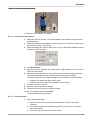
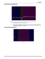
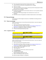
2.4.2 In-laboratory sensor stability analysis
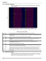
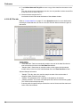
1. Select the Raw Plot tab to see the data.
2. Look at the data after 19 operation cycles to see if the data is stable.
20
Operation
Figure 14 Example of stabilized data
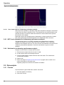
3. If the data is stable, go to the next section.
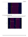
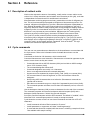
4. If the data is not stable, refer to Prepare to prime the sensor on page 9 and do the
steps again to make sure the sensor is set up correctly and has not pulled in any air,
which will give data that is not accurate.
Figure 15 Bubbles the sample line
21
Operation
Figure 16 Shifting baseline
2.4.2.1
Use of water tanks for in-laboratory performance analysis
When the sensor operates in a laboratory water tank, temperature changes or a decrease
in water flow can cause air bubbles to form. The manufacturer recommends that the user
operates a pump to circulate the water that crosses the sensor intake areas to prevent
the collection of air bubbles.
Data output values may change because of adsorption or primary production of a water
tank. The manufacturer recommends that the user validates the water in the tank.
2.4.3 NIST check standards for in-laboratory performance analysis
The manufacturer uses a 5.3 µM NIST-traceable check standard that is used after
calibration and before servicing to check the sensor's calibration. This 5.3 µM check
standard is also shipped to the user. The user can check the calibration of the sensor and
validate any lab-prepared standards. Contact the manufacturer to get more check
standard.
2.4.4 Solutions for in-laboratory performance analysis
Change to a new solution to analyze with the sensor.
1. Disconnect the sample inlet tube from the "S" barb.
2. Let the solution drain into the sample reservoir.
3. Flush the inside and the outside of the tube with clean water. The manufacturer
recommends 18 MOhm.
4. Shake to dry.
5. Refer to the steps in Prepare to prime the sensor on page 9 and be careful to not
make more bubbles in the intake tube.
Degassing sample can minimize the formation of bubbles.
2.5 Data analysis
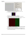
2.5.1 Files tab
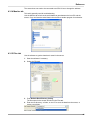
Use the software to get the data that is saved in the sensor.
1. Start the software if necessary.
2. Select the Files tab.
22
Operation
3. Push Refresh Root Directory Listing.
The files saved in the sensor will show in the Files tab.
4. Enter the file directory, or folder, on the PC to save the data from the sensor, or
create a new folder.
5. Push Offload Selected File(s)/Dir to move a copy of the data from the sensor to the
PC.
The user can save only one directory at a time, but it is possible to select several files
at the same time to save to the PC.
6. Monitor the data saved to the PC.
Look at the Current File area at the bottom of the software window.
23
Operation
2.5.2 Operation sequence
This section describes how the sensor calculates phosphate and how to interpret the
quality of the data.
Table 2 Cycle output periods
1
Blue
Pre-analysis flush period. The sample pump operates. Referred to as the "baseline."
2
Red
Ambient read period. Used for 100% transmittance without any absorption from phosphate reaction. No
pumps operate.
3
Green
Sample mix period. The sample pump and both reagent pumps operate.
4
Purple
Sample read period. No pumps operate. The reaction curve color develops. Counts decrease until
complete.
The white circle and number show the signal used as the sample transmission.
5
Blue
Post-analysis flush period. The sample pump operates. Output counts spike then increase to
approximately the baseline value.
6
Red
Spike ambient output period. No pumps operate.
7
Green
Spike mix period. The sample pump, both reagent pumps, and the calibration standard pump operate. A
known amount of phosphate is added to the sample.
8
Purple
Spiked sample read period. No pumps operate. Signal output counts decrease because there is more
phosphate added to the sample. This means more color develops and the transmission is lower.
9
Blue
Final flush period. The sample pump operates. As with the other flush periods, the output returns to a
baseline value.
2.5.3 Blank run example
A clean sensor will usually have a decrease in counts as it is conditioned. When the user
calibrates the sensor there is a shift in ambient read counts from run to run, or a slight
shift in the pre- and post-analysis rinse baseline of 50–100 counts.
24
Operation
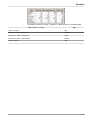
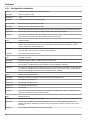
2.5.4 Good quality calibration data
Data such as the seven overlaid lines below shows good data. The lines show flat, stable
flush periods, downward spike during mixing, no signs of bubbles, and all seven lines
agree well.
25
Operation
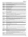
2.5.5 Bad data
The graph below is an example of bad data caused by bubbles.
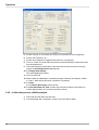
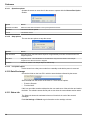
2.6 Data QA/QC
Select QA/QC File Plot tab to make an analysis of the quality of the data collected by the
sensor. Use the software to open and look at the data in a number of files. There are
algorithms in the software that let the user compare elements of the collected data as
"good," "bad," "suspect," or "not evaluated."
2.6.1 Open data files for analysis
The user can select a number of data files for analysis. Note that the more files that are
selected, the more time it takes the software to process the data.
1. If necessary, start the software.
2. Select the QC Plot tab.
3. Push the three dots to look for the directory with the data to look at.
4. Go to the File menu, then Load File(s).
5. Select the files to look at.
6. Push Open.
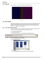
The Analysis Plot window opens and shows the selected graph.
26
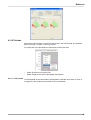
Operation
7. Look at the summary graph in the QC Plot tab of the software. Each of the files that
were selected to offload shows as a green, yellow, or red dot.
•
•
•
•
green dot: the file has no suspect or bad test parameters.
yellow dot: the file has one or more test parameters that are suspect.
red dot: the file has one or more test parameters that are bad.
blue dot: the data is saved for analysis, but the related raw data file has not yet
been read for analysis.
The blue dotted line shows which graph displays in the Analysis Plot window.
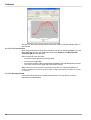
2.6.2 Compare data files
Use the information in the QC Plot tab to compare data files and make analyses of each
file. Use the values of the test parameters to help make a decision about the quality of the
data.
1. If necessary, open the files to examine. Refer to the previous section Open data files
for analysis on page 26 for details.
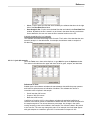
2. Look at the summary graph in the QC Plot tab.
3. Select one of the dots in the graph to open a data file in the Analysis Plot window.
27
Operation
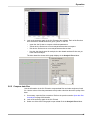
4. Look at the "Test," "Flag," and "Value" information.
In the example above, the "Mixing Spike" shows a "Suspect" "Value" of 79.
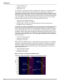
5. Look at the data in the Analysis Plot window.
Note the spike in the "Mixing" period (green background).
6. Put the cursor in the graph above and to the left of the spike. Drag the pointer
diagonally down and to the right to zoom in on the spike.
The spike is from approximately 2960 to 2880, a distance of 79 counts. It is shown as
"Suspect" in the "Mixing Spike" row of the table in the PO4 QC tab.
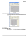
7. Push Auto Range in the Analysis Plot window to change the plot back to the default
scale, or drag the pointer from the lower right to the upper left (the opposite direction
from step 6) to return the graph to the default view.
8. Go to Tools, then Options, or enter Alt-O, to open the Cycle Host Options window.
The user can look at and change the values in this window. Push Reset to Defaults to
return to the manufacturer-set values.
28
Operation
The ranges of values for "Good," "Suspect," or "Bad" are given in the table below.
Value (output from sensor)
Flag
Value < Min Sus
Bad
Min Sus <= Value < Min Good
Suspect
Min Good <= Value <= Max Good
Good
Max Good < Value <= Max Suspect
Suspect
Value > Max Sus
Bad
29
Operation
30
Section 3
Maintenance
CAUTION
Wear Personal Protective Equipment (PPE) to remove or replace cartridges. PPE includes a lab
coat or smock, gloves, safety glasses.
PPE includes a laboratory smock, safety glasses, and gloves.
Replace the Cycle reagent cartridges and intake filters approximately every
1000 samples, and clean the optics flow path. Change the battery core of the battery
pack if that is the power source for the Cycle.
The sensor is calibrated to output a reactive phosphate concentration in user-defined
units of µM, mg/L, or mgP/L. The sensor will operate for approximately ten 1000-sample
deployments between service and re-calibration by the manufacturer.
1. Put the sensor on its side and use a Phillips screwdriver to remove the seven screws
that attach the protective cover to the sensor.
Figure 17 Protective cover removed
2. Support the bottom of the sensor and lift into a vertical position.
3. Pull the sleeve up and off the sensor. Keep the sleeve and the screws.
3.1 Clean and lubricate bulkhead connector
Lubricate the contacts of bulkhead connectors at regular intervals with pure silicone spray
only. Allow the contacts to dry before they are connected.
Make sure that the pins have no corrosion, which looks green and dull. Make sure that
the rubber seals on the pins are not delaminated. Connectors should connect smoothly
and not feel "gritty" or too resistant.
The manufacturer recommends 3M™ Silicone Lubricant spray (UPC 021200-85822).
Other silicone sprays may contain hydrocarbon solvents that damage rubber.
DO NOT use silicone grease. DO NOT use WD-40®. The wrong lubricant will cause
failure of the bulkhead connector and the sensor.
3.2 Clean macro-fouling
Wash and scrape clean any macro-fouling from the sensor to keep it in good condition.
Do not wash with a pressure-washer. Remove any anti-fouling tape before the sensor is
returned for servicing.
3.3 Clean sensor flow paths with cleaning solution
CAUTION
Do not operate the sensor with Micro-90® in it. It can damage the sensor.
31
Maintenance
CAUTION
Make sure all of the Micro-90® is flushed out of the sensor.
Clean the flow paths between each deployment with a 2% cleaning solution of Micro-90®
or Liqui-Nox® to keep the optics clean from the products of chemical reactions, which can
cause a decrease in sensitivity. Both solutions are available from various scientific supply
companies.
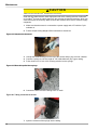
1. Make sure that the sensor is connected to a power supply and a PC with the Cycle
software on.
2. Pull the sample tubing straight off the hose barb to disconnect.
Figure 18 Sample tube loosened
3. Unwrap the exhaust tubing from the top of the sensor and put one end into a beaker.
4. Connect a syringe to a 25 cm length of 1/8" inside diameter (ID) Tygon® tubing.
5. Pull a minimum of 10 mL of 2% cleaning solution into the syringe.
Figure 19 Micro-90® pulled into syringe
6. Connect the other end of the tubing to the "S" barb.
Figure 20 Tubing connected to sensor
7. Inject the contents of the syringe into the tubing.
32
Maintenance
Figure 21 Tubing in cleaning solution
8. Disconnect the syringe and put the tubing it was connected to into the bottle of
cleaning solution.
9. Go to the Settings tab of the Cycle software and push Flush.
The sensor takes 5 minutes to fill with the cleaning solution.
10. Let the solution soak in the sensor for approximately ½ hour to 1 hour.
3.3.1 Clean flow paths with bleach solution
WARNING
Bleach is caustic. Wear nitrile gloves and safety glasses and work in a well ventilated area to use
bleach.
WARNING
Never mix bleach with ammonia. It can make dangerous gasses.
WARNING
Obey the safe handling and disposal instructions on the bleach containers.
CAUTION
Do not operate the sensor with bleach in it. It can damage the sensor.
NOTICE
Do not pre-dilute bleach. It will go bad. Only use bleach well before the expiration date on the
container.
It may be necessary to clean the optics with a bleach solution if the data output of the
sensor does not increase by approximately 2500 counts after it is cleaned with the
Micro-90® solution.
Table 3 Bleach dilutions
Description
Dilution
Clorox® Pro Results (concentrated outdoor)
9:1
Clorox®
2:1
Regular
Ultra
none
A 9:1 dilution is 9 parts water to 1 part bleach. For a 40 mL beaker, the solution is 4 mL of
outdoor bleach, 36 mL of water.
33
Maintenance
1. Make sure that the sensor has been flushed with clean water.
2. Do the procedures in the section on Clean sensor flow paths with cleaning solution
on page 31 but use bleach, not Micro-90®.
3. When the bleach flush procedure is complete, make sure to thoroughly rinse the flow
paths with clean water.
3.4 Flush cleaning solution from flow paths
1. Rinse the inlet tubing or get a new length to connect to the "S" inlet.
2. Fill a clean beaker with approximately 100 mL of clean water and put the other end of
the tubing in the beaker.
3. Go to the Settings tab of the Cycle software and push Flush.
4.
5.
6.
7.
8.
9.
a. Pull the inlet tubing out of the beaker of water. Let approximately 2 cm of air into
the tubing.
b. Put the inlet tubing back in the beaker. Let approximately 2 cm of water into the
tubing.
c. Do the two steps above until the inlet tubing is filled with 2 cm sections of air and
water.
Put the end of the outflow tubing in the beaker again.
Attach a syringe with a Luer® lock to a 1/16" hose barb and then the outflow tube on
the sensor.
Pull the plunger to the 15 mL mark to fill the syringe.
Push Flush if necessary.
Remove the syringe and put the inlet tubing in the waste beaker.
Push Flush two more times to make sure the sensor has been flushed three times.
The sensor is now clean.
Disconnect the syringe and tubing and the inlet tubing from the "S" port.
3.5 Replace reagent cartridges
CAUTION
Wear Personal Protective Equipment (PPE) to remove or replace cartridges. PPE includes a lab
coat or smock, gloves, safety glasses.
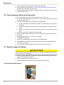
1. Remove the blue calibration cartridge first. Press the stainless steel coupler on the
bottom of the cartridge to release it.
2. Slide the cartridge up and off the guide pins.
3. Pull the cartridge away from the housing and set the cartridge aside.
Figure 22 Blue cartridge removed
34
Maintenance
4. Remove the yellow and then the red cartridges.
5. Install new cartridges. Refer to the section on Assemble the sensor on page 5 for
details on this procedure.
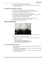
3.6 Replace intake filter and screen
1.
2.
3.
4.
5.
6.
7.
8.
9.
10.
Disconnect the tubing from the top of the two stainless steel filters.
Remove the two screws that hold the intake filter holder to the base plate.
Remove the filter housing from the base plate.
Loosen the set screw that holds the intake filter in the holder.
Push (gently) on the tubing fitting of the filter to remove the filter from filter housing.
Remove the plastic spacer from the bottom of the filter.
Remove the copper screen from the base plate.
Replace the copper screen with the new screen that came with the filters.
Install the plastic spacer onto the bottom of the new filter.
Put the new filter into the filter holder.
Figure 23 10 µm filter installation
11. Tighten (gently) the set screw that holds the filter in place. Do not over-tighten.
12. Install the filter and the holder onto the base plate.
a. Start one screw. Hold the other side of the filter holder stable with a thumb or
finger.
b. Start the second screw.
c. Make sure the screws are tightened evenly.
Try to keep the filter holder parallel to the base plate.
d. Tighten to hand-tight. Do not tighten too much.
3.7 Prime sensor with vacuum
1. Attach the Luer-lock and the 1/16" ID barb adapter to the exhaust tubing and to the
supplied syringe.
2. Attach the syringe with the adapter to the outlet of the 1/16" ID sensor effluent tubing
that comes out of the top end flange.
3. Under the Settings tab, make a check in the "Cal" box and set the calibration pump to
operate for 100 pump cycles.
35
Maintenance
4. Push Run Pump(s).
5. While the pump is in operation, pull a light vacuum, approximately 1/5 (10 mL) of the
full travel of the plunger.
6. After the pump has operated for 100 cycles, make sure that the reagent tubing that
connects the cartridges and the inlet barbs does not have any air bubbles.
Look at the tubing from the reagent cartridges to the manifold to check for bubbles.
7.
8.
9.
10.
• If bubbles are present, do steps 4 and 5 again.
• If bubbles are small, it may not be possible to remove them.
Do steps 3–5 with R1 and R2.
Disconnect the tubing from the syringe.
Put the end of the tubing into an empty receptacle.
Go to the Settings tab and push Flush.
The Sample fluid opening is primed.
3.8 Send reagent cartridges back to manufacturer
CAUTION
Wear Personal Protective Equipment (PPE) to remove or replace cartridges. PPE includes a lab
coat or smock, gloves, safety glasses.
Return Policy: The manufacturer will recycle cartridges sent back by the user.
The manufacturer will only accept red reagent cartridges that have been drained
and flushed.
Do the steps below to prepare the red cartridge to send back to the manufacturer.
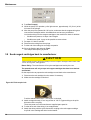
1. Disconnect the red cartridge from the sensor if necessary.
2. Make sure the cartridge is unlocked.
Figure 24 Fluid coupler lock
Push the stainless steel tab in. The coupler is unlocked.
3. Attach an approximately 15 cm long section of 1/8" ID Tygon® tubing to the quickdisconnect inline coupling.
These two parts are in the manufacturer-supplied spare parts kit.
4. Put the other end of the tubing in an empty beaker.
5. Attach the tubing with the quick-disconnect coupling to the red reagent cartridge.
Any fluid in the cartridge will drain into the beaker.
36
Maintenance
6.
7.
8.
9.
10.
11.
12.
13.
Fill a syringe with DI water and fill the cartridge with the water.
Disconnect the quick-disconnect coupling body from the cartridge.
Shake the cartridge.
Connect the quick-disconnect coupling to the tubing and the cartridge again and drain
the DI water in the cartridge into a beaker.
Do steps 6–9 two more times.
Put the empty cartridges into a new box with a minimum of 5 cm of protective material
around the cartridges.
Send all three of the empty cartridges to the manufacturer for credit on new
cartridges.
Follow all local laws and regulations to discard the waste water from the cartridges.
3.9 Sensor storage
Always flush out all of the reagents in the sensor. Push Flush in the Settings tab to do
this procedure.
3.9.1 Short-term storage
Make sure that the sensor is clean and has been flushed before it is put into storage for
as long as a month.
1. Clean any biofouling from the protective sleeve.
2. Clean and flush the sensor. Refer to the steps in Send reagent cartridges back to
manufacturer on page 36 for details on cleaning the red cartridge.
3. Make sure the cartridges are installed on the sensor.
4. Wind the outlet tubing around the eye bolts.
3.9.2 Long-term storage
CAUTION
The waste solution from the sensor cartridges is Hazardous Waste. Follow the applicable
regulations to discard the solution.
CAUTION
Wear Personal Protective Equipment (PPE) to remove or replace cartridges. PPE includes a lab
coat or smock, gloves, safety glasses.
Make sure that the sensor is clean and has been flushed before it is put into storage for
as long as several months.
1. Clean any biofouling from the protective sleeve.
2. Clean and flush the sensor. Refer to the steps in Send reagent cartridges back to
manufacturer on page 36 for details on cleaning the red cartridge.
3. Use the syringe to fill the cartridge with DI water.
4. Attach the Tygon® tubing to R2.
5. Turn the sensor on.
6. At the Settings tab, type 200 in the number of pumps area.
7. Push Run Pump(s).
8. Fill and flush each cartridge.
Keep flow passages filled with DI water.
9. Wrap the outlet tubing around the eye bolts.
10. Keep the reagent cartridges in a refrigerator.
37
Maintenance
11.
12.
13.
14.
15.
38
Replace any worn parts.
Lubricate the bulkhead connectors.
Attach the protective dummy plugs and lock collars.
Attach the protective sleeve to the sensor.
Put the sensor in its case for safe storage.
Section 4
Reference
4.1 Description of nutrient units
Nutrient units express the amount of something, usually moles or mass, relative to the
volume it is in. Many researchers and scientists use micromoles per liter (µM), a unit that
is independent of mass and useful for stoichiometric calculations.
Most freshwater monitoring programs and many researchers use units of milligrams per
liter. This unit is almost always expressed as milligrams of relevant atoms per liter—for
example, milligrams of phosphorus (P) per liter, rather than milligrams of phosphate per
liter. Although phosphate (PO4) is the most prevalent form of phosphorus, this unit is
frequently used as a means of easily keeping track of total phosphorus loading. Because
milligrams per liter is a mass-based unit and the mass of P and PO4 are different, this
difference is very important to prevent mistakes. Milligrams per liter is also typically
referred to as parts per million (ppm), the mass of P relative to the mass of water.
The Cycle PO4 sensor measures soluble reactive phosphate and displays units in
micromolar (µM) or milligrams of phosphorus per liter (mgP/L). The Cycle PO4 sensor
also displays units in milligrams phosphate per liter (mg/L or mgPO4/L). MgPO4/L is not
commonly used in environmental analysis. Standards, such as the Hach® 0.5 mg/L
standard, are sometimes expressed in this unit.
4.2 Cycle commands
The user can use commands as an alternative to the host software to communicate with
the Cycle sensor. Refer to the information below for details about how to use the
commands.
Commands are limited to 160 characters, which includes the $.
Command characters are case-insensitive. Characters are converted to uppercase by the
sensor, but are shown as they are entered.
•
•
•
•
•
•
•
•
•
Commands start with an ASCII $ character (0x24) and end with an ASCII carriage
return <CR> character (0x0d)
The command designator follows the $.
Command designators are usually 3 or 4 characters.
One or more arguments follow the command designator.
Arguments can be separated by a space (0x20), a tab, (0x09), or a comma (0x2c).
If a command does not need an argument, a <CR> line terminator follows the
designator.
Non-printing ASCII characters that occur before the $ that starts a command are
ignored and not shown.
More than one command can go on a single line if separated by semi-colons (0x3b).
The commands operate until there are more than 160 characters per line, or there is
an error.
Use the backspace character (0x08) to remove characters from the end of the command.
The command interpreter will show the backspace and send a space (0x20) and a
backspace (0x08) character to "delete" the removed character.
Set up the command interpreter with the SPR command. The default is "enabled," which
shows the PO4> command prompt when it is ready to accept commands.
Cycle shows the success or failure of user-issued commands and end with <CR><LF>
characters.
•
•
•
Invalid commands will show "Bad command or file name."
Invalid parameters, or arguments, will show "invalid argument(s)."
A command that cannot be accepted while the sensor is collecting a sample will show
"Not available while sample running."
39
Reference
4.2.1 Configuration commands
CAS
Constant A-Star value (manufacturer's scale factor)
Description
Get the constant a* value
Argument 1
none
Response
The constant a* value to two decimal places
CLK or TIME
Get/set the sensor's internal clock or date
Description
Get/set the sensor's internal clock or date
Argument 1
The new time in hh:mm:ss (24-hour clock) or the new date (mm/dd/yy) if both the date and time are set.
Argument 2
The new time in hh:mm:ss (24-hour clock) if both the date and time are being set.
Response
The current or new date and time in mm/dd/yy hh:mm:ss format. The hours are in a 24-hour format. The
date and time are separated by a tab character, (0x09), not by a space.
CNT
Sample CouNTer
Description
Get/set the current or most recent sample number. This is the number used in the raw file naming
format. When the sample counter is set, the next sample run is the newly set count plus 1. Set this
value to 0 at the start of each deployment.
Argument 1
New count value for the number of data samples completed. Must be followed by a /S switch to change
the count. Set to one less than the number of the next sample.
Response
The current or new sample counter.
CSF
Cal Spike Frequency
Description
Get/set the frequency that a cal spike is done. The default is 6.
Argument 1
The new frequency. The next data sample after this command will do a cal sequence. Allowed values
are 1 to 32767. If a data sample is being collected, the new value will not change it.
Response
The current or new cal frequency followed by the number of data samples before the next cal spike. The
two values are separated by a space character (0x20). A value of zero for the number of data samples
before the next cal spike means that the next sample will run a cal spike.
DCA
Deployment Cartridge Amounts
Description
Get/set the quantity of chemicals in the sensor at the start of a deployment.
Argument 1
The calibration standard in mL.
Argument 2
The quantity of reagent 1 in mL.
Argument 3
The quantity of reagent 2 in mL.
Argument 4
/S safety flag
Response
The current or new cartridge quantities to three decimals in milliliters at the start of a deployment. The
values are separated by a space character (0x20).
DSD
Data SubDirectory
Description
Get/set the subdirectory used to save data.
Argument 1
The name of the subdirectory without the root directory (e.g. C:\). Only subdirectories of the root
directory are allowed. Subdirectory names can be no longer than 8 characters. Only a–z and 0–9 are
permitted.
Response
The message "resets" when the command is completed.
40
Reference
DSI
Device Specific Information
Description
Get device-specific pump volumes, the optical pathlength, the PO4 offset, and the scale factor.
Argument 1
The ambient (sample) pump volume in µL.
Argument 2
The pump volume of the calibration standard in µL.
Argument 3
The pump volume of reagent 1 in µL.
Argument 4
The pump volume of reagent 2 in µL.
Argument 5
The PO4 offset volume in µM.
Argument 6
The calibration offset in µL.
Argument 7
The cell pathlength in cm.
Response
The current value. The arguments in this table show in order from argument 1 to argument 7, separated
by space characters (0x20). The pump volumes and pathlength show to two decimal places. The offsets
show to four decimal places.
EUF
Engineering Units Format
Description
Get/set the units to use for engineering units output.
Argument 1
The units to use. 0 = microMolar (µM). 1 = milligrams of phosphate per liter (mg/L). 2 = mg of atoms of
phosphorus per liter measured in the form of reactive phosphate (mgP/L).
Response
The new or current values as "µM," "mg/L," or "mgP/L."
IDT
IDle Timeout
Description
Get/set the communication idle time in seconds. If no communication is received within this time period
while a data sample is not running, the sensor goes back to a low power "sleep" state.
Argument 1
The new communication idle timeout in seconds. The range is 5 to 4924.
Response
The new or current idle timeout in seconds.
INT
sampling INTerval
Description
Get/set the time period between data samples, referenced from one start time to the next.
Argument 1
The interval in seconds or minutes:seconds or hours:minutes:seconds. If 0, the sensor will collect one
data sample and then stop.
Response
The new or current sample interval as hh:mm:seconds.
NOS
Number of Samples
Description
Get/set the number of data samples (includes the current data sample) to collect before the sensor
stops.
Argument 1
The number of data samples to collect. The default is -1, which sets no limit to the number of data
samples.
Response
The new or current number of data samples to collect.
OPD
Output PerioD
Description
Get/set the data output interval. Use with SDO command that looks like the old sensor data output
format to specify how often a data sample is sent from the sensor. The default is 5. This value also
specifies how often the raw signal data is written to the raw data files.
Argument 1
The new output interval. Makes the old version data output to show every nth LED cycle.
Response
The new or current period of output.
41
Reference
RAT
Serial port RATe
Description
Get/set the baud rate for the serial port.
Argument 1
The new rate. Values are 9600, 19200, 38400, 57600, and 115200.
Response
If argument 1 is used, the response is "Changing rate to arg1. Hit <Enter> when ready." If no argument
is used, or after <Enter> is pushed, the new baud rate shows. Note that data samples collected at a
baud rate other than 19200 may result in bad data. The baud rate cannot be changed while data is
being collected.
SDA
SDI Address
Description
Get/set the SDI bus address for the sensor.
Argument 1
The new SDI sensor bus address as an integer from 0 to 9.
Response
The current or new address This will also show an address change that was sent via the SDI bus.
SDO
Output mode
Description
Get/set the format of the data that is output. The default mode of 0 is the same as the old data output
format with final engineering units added at the end of each sequence. Modes 1 and 2 are for use by
the manufacturer. Mode 3 shows only the engineering units of data at the end of a data sequence.
Mode 4 shows no engineering units data.
Argument 1
The mode of operation to use.
Response
The current or new mode of operation.
SPR
Set PRompt
Description
Turn the command prompt of PO4 on or off.
Argument 1
1 = turn on command prompt, 2 = turn off command prompt.
Response
The current or new command prompt shows as either "on" or "off." When the prompt is turned off, there
is no prompt after a response. When the prompt is turned on, there is a PO4 prompt after a response.
STO
STOre configuration to flash
Description
Saves the current configuration values to a non-volatile flash memory. This command automatically
executes when a low input power fault happens, before the sensor enters a low power state, or when
the user exits to PicoDOS.
Argument 1
None
Response
The message "written" on a complete command.
SUD
Start time and date
Description
Get/set the time and date for the first or next data collection sample or for a scheduled pump prime
cycle. No arguments returns the date and time for the next scheduled data collection sample or none. If
NOS is 0, it will automatically be set to -1.
Argument 1
The start date as m/d/y (optional) or /P to show the date and time (or none) of the scheduled pump
prime cycle.
Argument 2
The start time (h:m:s) or 0 to stop data collection.
Argument 3
/P to apply the preceding time or date and time to the pump prime cycle start time.
Response
The current or new mode of operation.
UPC
UPS Count
Description
Get the number of UPS cycles.
42
Reference
Argument 1
None
Response
The number of UPS cycles that have happened from low-power faults.
WKM
External wake mode
Description
Get/set the operation when an external wake signal happens on pin 1. The default = 0 brings the sensor
out of a low power mode. Mode 1: starts a data collection (sample) sequence. Mode 2: sensor to show
the most recent data collected.
Argument 1
The wake-up mode.
Response
The new or current wake mode. 0 = off. 1 = start on wake signal. 2 = show the most recently completed
sample (GLSO) on the wake signal.
4.2.2 Operation commands
FLT
Fault Status
Description
Show any fault conditions.
Argument 1
none
Response
A four-character hexidecimal value that shows the fault status. The value 0000 shows that there are no
faults.
Table 4 Fault conditions
Bit field
Fault
0x0001
Invalid values at startup. The default values are used.
0x0002
The values used at startup were not saved. Some values may not be in effect.
0x0004
Invalid operational values at startup. The default values are used.
0x0008
The operational values used at startup were not saved. Some values may not be in effect.
0x0010
The saved data subdirectory did not exist at startup and could not be made.
0x0020
Communication to the gas gauge controller was not made.
0x0040
SYS.QPBCS is not set correctly.
GLSO
Get Last Sample Output
Description
Get the data for the most recently completed or ended sequence of data collected.
Argument 1
none
Response
The most recently completed or ended sample collection sequence followed by two pair of <CR><LF>
characters. Refer to Error: Reference source not found for the data format.
KCO
Description
Operates a user-specified number of cycles to flush the sensor after the reaction is complete and the
analytical signal is selected
Argument 1
Positive integer for cycles at 2 Hz.
Response
The pumps operate for a user-specified number of cycles. The manufacturer recommends 120.
LSS
Last Shutdown State
Description
Get the status of the last shutdown.
43
Reference
Argument 1
none
Response
The message "ok" if the shutdown was via the "XIT" command or "power failure" if the last shutdown
was from a power fault.
ONT
Run Time/Power Consumption
Description
Get/set the total "on" time for the sensor. This number is usually reset when a new battery is connected.
Argument 1
The new "on" time, in seconds.
Argument 2
/S = safety flag.
Response
The current/new "on" time, in h:mm:ss. The hours field is from 1 to 10 characters.
PRI
Prime
Description
Do the priming sequence immediately.
Argument 1
1 = starts the priming sequence. 0 = starts the flush process while the priming sequence occurs.
Response
The status of the priming sequence. The message "on" or "off" will show if no arguments are made. The
message "priming" shows if priming is started.
RUN
Run
Description
Start a new data sample sequence now. If NOS is 0, it will automatically set to -1.
Argument 1
/P = start a priming sequence.
Response
The message "Running" shows if a data sample sequence is started. The message "Priming" shows if a
priming sequence is started.
SDS
SDI Status
Description
Get the status of the SDI interface board.
Argument 1
none
Response
VER:n.n c enabled|disabled. n.n = the interface3 board version number. c = the code that shows the
status of operation, and either enabled or disabled to show if the board is on or off.
0–8 = the board is being started, or there is a problem.
9 = the board is OK but does not have power from the SDI bus.
10 = there is no SDI interface board, or it is not in communication.
11 = the board is OK and has power from the SDI bus.
SLP
Sleep
Description
Put the sensor in a low power "sleep" mode for a specified time, until a specified time, or indefinitely.
Use the serial port or the external wake signal to put the sensor in a "ready" mode. Some characters are
baud rate-dependent and cannot be used to "wake" the sensor. The character that is used to "wake" the
sensor is not buffered for input. The manufacturer recommends that the user does an RS232 break of at
least 500 ms to "wake" the sensor.
Argument 1
The number of seconds to be in a low power state. No argument = stay in low power until the next data
sample time occurs.
Response
The message "Sleeping <CR><LF>" shows. When argument 1 is used, or if the sensor is going to
collect a data sample, the message " for n seconds <CR><LF>" shows, where "n" is the smaller of the
value of the commanded interval or the time to the next data sample.
44
Reference
STP
SToP
Description
Cancel a sample sequence and flush the sensor, or stop immediately. If the flush occurs, NOS goes
down, as though a whole sample was completed. If a sample is not being collected, the SUD and
SUD /P move to 0 and the NOS value does not change.
Argument 1
no argument = the flush sequence occurs.
/I = the sample sequence stops. The NOS does not change, as though the sample sequence did not
occur.
Response
"Stopped" shows if there was no sample sequence.
"Flushing" shows if the user made the command without the /I argument.
"Stopping" shows if the user made the command with the /I argument.
TPC
Total Pump Counts
Description
Get the total number of pump actions by any or all of the pumps in the sensor. The pump counter is
reset when a new pump is installed.
Argument 1
none
Response
Shows the counts for the ambient (sample) pump, the calibration pump (blue), the reagent 1 pump,
(yellow), and the reagent 2 pump (red) separated by spaces. These are the total counts over the lifetime
of the pumps installed by the manufacturer.
TTS
Time To Next Sample Start
Description
Get the time until the start of the next scheduled sample sequence.
Argument 1
none
Response
Shows the time in h:mm:ss until the next sample starts. Shows a 0 if a sample is being collected, or -1 if
a sample is stopped.
VOL
Volumes Pumped/Deployment Pump Counts
Description
Get/set the volumes for all the pumps in the sensor for this deployment. An optional argument is /R /S =
resets all four pump volumes to 0.00.
Argument 1
Ambient volume from the pump in mL.
Argument 2
Calibration standard from the pump in mL.
Argument 3
Reagent 1 from the pump in mL.
Argument 4
Reagent 2 from the pump in mL.
Argument 5
/S = safety flag
Response
The current or new volumes in mL to three decimal places in the order above. The values are separated
by a space.
XIT | EXIT
Exit
Description
Stop the firmware application and go to PicoDOS. Scheduled samples are stopped. (Same as SUD 0).
Argument 1
none
Response
None from the sensor application. The PicoDOS start message shows at the current baud rate after
several seconds.
4.2.3 File commands
CPY
Copy
Description
Copy a file to a new filename or location on the flash drive. "Wildcards" (* and ?) are permitted. Note
that if a destination file already exists, it will be overwritten.
45
Reference
Argument 1
The file or files to be copied.
Argument 2
The destination of the copied file or files.
Argument 3
An optional /V command to verify the new file or files.
Response
The names of the source files, followed by <CR><LF> as they are copied. After the last file is copied, an
additional <CR><LF> shows, followed by "n files(s) copied" where "n" is the number of files copied. The
message is padded with spaces so that the number field is always eight characters wide and ends with
two <CR><LF>.
DEL
Delete
Description
Erase the specified file or files from the flash drive. "Wildcards" (* and ?) are permitted.
Argument 1
The file or files to be erased.
Response
"n" file(s) erased. n = the number of files erased. The response ends with two <CR><LF>.
DIR
Dir
Description
Get a list of the files in the directory. "Wildcards" (* and ?) are permitted. The "*" character = any group
of one or more alphanumeric characters. The "?" = any single alphanumeric character.
Argument 1
The directory to list, or /D for the "current" directory.
Argument 2
The optional filename pattern to list. For example, "*.txt"
Response
A list of the directory with the specified filters. If a file is being collected, it will list on the last line,
separated by a space from the preceding "Active file".
GET
Get File
Description
Get the specified file or files. "Wildcards" (* and ?) are permitted. The file move is stopped with an
RS232 break signal of 500 ms or longer. This is followed by the "checksum" for the characters that were
sent before the sensor got the break signal.
Argument 1
The files to be moved.
Response
All of the specified files will be moved. A header line comes before each file. The header line has the
filename, the number of the file being moved, from 1 to "n", the total number of files moved, the file size
in bytes, and the number of bytes that need to be moved. This information is separated by a space. The
whole file is moved and is followed by the CRC-32 "checksum" of eight hexidecimal characters. Data
being collected will stop while the file is moved. If GET is used the data output stream will have pauses
for the sensor's internal requirements.
REN
Rename
Description
Change the name of a specified file on the flash drive.
Argument 1
The path and the file to change.
Argument 2
The new path and the file name.
Response
<CR><LF>.
"Not found error" = the file does not exist.
"Rename error" = the file exists or there was another error.
RMD
Remove Directory
Description
Erase the specified sub-directory if it is empty. Note that an open subdirectory cannot be erased even if
it is empty. Use the DSD command to change the data sub-directory first.
46
Reference
Argument 1
Path to the empty directory to erase
Response
"Dir Removed"= directory is erased.
"error code" = directory does not exist.
"Dir not empty error" = directory is not empty.
TYPE
Type
Description
Shows the specified files from the serial port. There is no data verification or way to see the end of a file.
"Wildcards" (* and ?) are permitted.
Argument 1
The files to show.
Response
Directory, then filename, separated by a \ character, then <CR><LF>.
4.2.4 Miscellaneous commands
DAC
Set DAC output
Description
Set the level of output of the Digital-to-Analog converter to a specified level.
Argument 1
The 12-bit value shows in hexidecimal format from 0–fff.
Response
The new DAC level of output.
Table 5 Common DAC output voltages
Value
Approximate output voltage
0
0.00
333
1.00
400
1.25
666
2.0
800
2.5
999
3.0
c00
3.75
ccc
4.00
fff
5.00
DEV
Device Type
Description
Get the device-type and serial number of the sensor
Argument 1
none
Response
The device-type and the serial number of the sensor separated by a space. "PO4" = device-type.
"nnn" = three-characters, where "n" is a number fro 0–9.
H | HELP
Help
Description
Show the available commands
Argument 1
none
Response
See table below
Table 6 Summary of Commands
Type of command
C = Configuration
O = Operation
F = File
M = Miscellaneous
47
Reference
Type of
command
Command
Description
Type of
command
Command
Description
C
$CAS
const a*
C
$CCS
calibration concentration
C
$CLK
get/set date and time
C
$CNT
sample counter
F
$CPY
source destination
C
$CSF
calibration frequency
M
$DAC
set dac output
C
$DAT
get/set date and time
C
$DCA
get/set cartridge volumes
F
$DCS
default config
F
$DEL
file
M
$DEV
get device type
F
$DIR
/D for data dir
C
$DSD
data subdir
C
$DSI
device config
C
$EUF
get/set units format
O
$FLT
get fault status
F
$GET
get file(s)
O
$GLSO
get last output
C
$IDT
idle timeout
C
$INT
sample interval
O
$KCO
operate pumps to flush
O
$LSS
last shutdown state
C
$NOS
number of samples
O
$ONT
show on time
C
$OPD
output period
O
$PMP
operate pumps
M
$PRI
priming state
C
$RAT
get/set baud rate
F
$REN
oldname newname
F
$RMD
remove empty dir
O
$RUN
run sample
C
$SDA
SDI bus address
C
$SDO
output format
O
$SDS
SDI status
O
$SLP
low power sleep
C
$SPR
prompt on/off
C
$STO
store config info
O
$STP
stop sample
C
$SUD
start time/date
O
$TPC
get total pump counts
O
$TTS
time til start
F
$TYPE
dump file(s)
C
$UPC
get ups count
M
$VIN
get input voltage
O
$VOL
get volumes pumped
M
$VSN
show version info
O
$WKM
get/set wake mode
O
$XIT
exit to PicoDOS
PMP
Operate Pump(s)
Description
Operate the specified pumps for a specified number of cycles. Files are not made and data is not
collected. Use the STP/I command to stop a PMP command.
Argument 1
None to get the number of pump cycles left, or a decimal code that specifies which pumps to operate.
Set a bit position to 1 to start the pump.
Response
The number of pump cycles left. "Pumping Done" = pump operation is complete.
Code
Amb
Cal
R1
R2
Code
Amb
Cal
R1
R2
0
no
no
no
no
8
no
no
no
yes
1
yes
no
no
no
9
yes
no
no
yes
2
no
yes
no
no
10
no
yes
no
yes
3
yes
yes
no
no
11
yes
yes
no
yes
4
no
no
yes
no
12
no
no
yes
yes
48
Reference
5
yes
no
yes
no
13
yes
no
yes
yes
6
no
yes
yes
no
14
no
yes
yes
yes
7
yes
yes
yes
no
15
yes
yes
yes
yes
VIN
Input Voltage
Description
Get the input voltage to the sensor in volts.
Argument 1
none
Response
The input voltage to the sensor shows to two decimal places. It shows approximately 0.2 V lower than
the voltage supplied to the sensor.
VSN
Version
Description
Get the firmware version in the sensor.
Argument 1
none
Response
The firmware version. "n.nn" where "n" is a digit from 0–9.
4.2.5 SDI commands
The sensor supports all basic SDI-12 commands. Refer to the SDI-12 specification at
www.sdi-12.org for details of the command protocol. The SDI-12 has been tested with the
SDI-12 Verifier from NR Systems Inc. (http://www.sdi-12-verifier.com) with up to 1000 ft.
of 24-gauge cable for communication (NOT power). For any command not described
below, the sensor will respond according to the SDI-12 v1.3 specification.
Definitions
•
•
•
•
"a" is the sensor's SDI-12 address
<CRC> is the 3-character Cyclic Redundancy Check
<CR> is a Carriage Return character
<LF> is a Line Feed character
Table 7 SDI data formats
Index
Description
Format
1
Sample date
YY.MMDD
2
Sample time
HH.MMSS
3
Run number
dddd
4
PO4 concentration
d.dddd OR dd.ddd
Note that -99999 shows as the PO4 concentration (index 4) if
an unrealistic PO4 value is determined (a "nan" in the summary
file). This happens when a sequence is stopped early or the
calculation gives an undefined result.
5
Units of PO4 concentration
d
0 = specifies microMolar (µM)
1 = specifies milligrams phosphate per liter
(mg/L)
2 = specifies mg of atoms phosphorus per liter
measured in the form of reactive phosphate
(mgP/L)
49
Reference
Table 7 SDI data formats (continued)
6
Last sample status
d
0 = Initial flush
1 = Ambient read 1
2 = Mix ambient
3 = Ambient PO4 read
4 = Completed normal run
5 = Mid flush 2
6 = Ambient read 2
7 = Mix spiked
8 = Spiked PO4 read
9 = Completed spike run
7
battery voltage, volts
dd.d
Table 8 SDI Commands
Acknowledge Active (a!)
Response
a<CR><LF>
Purpose
verifies the SDI-12 address
Example
address = 0
SDI recorder sends 0!
sensor sends 0<CR><LF>
Address query (?!)
Response
a<CR><LF>
Purpose
shows the sensor's SDI-12 address
Example
address = 0
SDI recorder sends ?!
sensor sends 0<CR><LF>
Change address (aAb!)
Response
b<CR><LF>
Purpose
changes the sensor's SDI-12 address to "b". The default address is 0.
Example
address = 0
SDI recorder sends 0A1!
sensor sends 1<CR><LF>
address now = 1
Send identification (aI!) ("a, capital I, !)
Response
allccccccccmmmmmmvvv_ssssss_fffffff<CR><LF>
a = sensor address
Il (lowercase "L") = 2-character SDI-12 version. For example, "1.3" for version 1.3
cccccccc = 8-character manufacturer identification. For example, "WET LABS"
mmmmmm = 6-character sensor model. For example, "_CYCLE"
50
Reference
vvv = 3-character sensor version. For example, "PO4"
_ssssss = up to 6-character serial number field. Includes leading space
_fffffff = up to 7-character firmware version field. Includes leading space
Example
address = 0. serial number = 104. The firmware version is 1.03sd
SDI recorder sends 0I!
sensor sends 013WET LABS CYCLEPO4___104_1.03sd<CR><LF>
Start Measurement (aM!)
Start Measurement and Request CRC (aMC!)
Response
atttn<CR><LF>
Purpose
starts a measurement
Notes
a = address = (0–9)
ttt = measurement time in seconds. The sensor always sends 000.
n = 7. The number of measurement values the sensor makes and returns after subsequent Send Data
commands.
If a scheduled prime sequence is pending or in operation, the sensor will ignore the Start Measurement
and Start Measurement and Request CRC commands.
The sensor needs approximately 1800 seconds (30 minutes) to complete a
measurement. The SDI-12 specification allows measurement times from 000 to 999. The
sensor uses a "save and forward" technique to work around this limitation. The sensor
always sends the measurement time as 000 seconds. Measurements are saved in firstin-first-out (FIFO) memory. If the SDI recorder sends a Start Measurement command and
subsequent Send Data command, the sensor sends the next set of data in the FIFO. If
there is no saved data, the sensor sends a null response (a <CR><LF>). The data
recorder or data processor program needs to handle these values appropriately.
The sensor has the same response to Start Measurement and Request CRC except that it appends a 3-byte CRC to the data
when it responds to the Send Data command.
Example
address = 0
SDI recorder sends 0M!
sensor sends 00007<CR><LF>
SDI recorder sends 0MC!
sensor sends 00007<CR><LF>
Refer to the Send Data command for examples of the commands that come after either
the aM! or aMC!
Start Concurrent Measurement (aC!)
Start Concurrent Measurement and Request CRC (aCC!)
Response
atttnn<CR><LF>
Purpose
starts a measurement
Notes
a = address = (0–9)
ttt = measurement time in seconds. The sensor always sends 000.
51
Reference
nn = 07. The number of measurements the sensor will make and return after subsequent Send Data
commands.
If a scheduled prime sequence is pending or in operation, the sensor will ignore the Start Measurement
and Start Measurement and Request CRC commands.
Start Concurrent Measurement (aC!). Has 70 characters.
Start Measurement (aM!). Has 35 characters.
Example
address = 0
SDI recorder sends 0C!
sensor sends 000007<CR><LF>
SDI recorder sends 0CC!
sensor sends 000007<CR><LF>
Send Data commands that come after either the aM! or aMC! commands:
Send Data (aD0!–aD1!)
Response
a<values><CR><LF> or a<values><CRC><CR><LF>
Purpose
sends data to the SDI recorder
Notes
aD0! after aM!
35 characters are allowed. For the sensor the response is 6, the first 6 values in the SDI data format
table. There is not space in the 35-character field for 7 values. If a subsequent aD1! command is sent
the sensor will send the seventh value, battery voltage.
aD0! after aC!
70 characters are allowed. For the sensor the response is 7 values. There is space in the 70-character
field for 7 values. The recorder does not need to send an aD1! command because all 7 values are sent
after the aD0! command.
aD0! and aD1! after an aM! command (Assume the sensor is set to address 0.)
Example 1
address = 0
values from the previous measurement:
sample date
11.0705
sample time
06.0708
run number
0500
PO4 concentration
12.345
units of PO4 concentration
0
last sample state
9
battery voltage
12.1
SDI recorder sends 0M!
sensor sends 00007<CR><LF>
SDI recorder sends 0D0!
sensor sends 0+11.0705+06.0708+0500+12.345+0+9<CR><LF>
recorder sends 0D1!
sensor sends 0+12.1<CR><LF>
52
Reference
aD0! and aD1! after an aMC! command
Example 2
address = 0
values from the previous measurement:
sample date
11.0706
sample time
06.0809
run number
0501
PO4 concentration
12.678
units of PO4 concentration
0
last sample state
9
battery voltage
12.0
SDI recorder sends 0MC!
sensor sends 00007<CR><LF>
SDI recorder sends 0D0!
sensor sends 0+11.0706+06.0809+0501+12.678+0+9GTu<CR><LF>
recorder sends 0D1!
sensor sends 0+12.0GFS<CR><LF>
aD0! after an aC! command
Example
address = 0
values from the previous measurement:
sample date
11.0707
sample time
06.0910
run number
0502
PO4 concentration
12.901
units of PO4 concentration
0
last sample state
9
battery voltage
11.9
SDI recorder sends 0C!
sensor sends 00007<CR><LF>
SDI recorder sends 0D0!
sensor sends 0+11.0707+06.0910+0502+12.901+0+9+11.9<CR><LF>
aD0! after an aCC! command
Example
address = 0
values from the previous measurement:
sample date
11.0708
sample time
06.1011
run number
0503
PO4 concentration
12.234
53
Reference
units of PO4 concentration
0
last sample state
9
battery voltage
11.8
SDI recorder sends 0CC!
sensor sends 00007<CR><LF>
SDI recorder sends 0D0!
sensor sends 0+11.0708+06.1011+0503+12.234+0+9+11.8FZH<CR><LF>
Continuous Measurement (aR0!)
Continuous Measurement and Request CRC (aRC0!)
Response
a<values><CR><LF> or a<values><CRC><CR><LF>
Notes
sensor sends the last measurement data stored in the FIFO. The format is the same as aD0! after an
aC! or aCC! command. If there is no data in the FIFO, the sensor sends the last data record sent.
the Continuous Measurement command does not start a measurement. It sends data from a previous
measurement.
aR0!
Example 1
address = 0
values from the previous measurement:
sample date
11.0710
sample time
06.1213
run number
0505
PO4 concentration
12.890
units of PO4 concentration
0
last sample state
9
battery voltage
11.6
SDI recorder sends 0R0!
sensor sends 0+11.0710+06.1213+0505+12.890+0+9+11.6<CR><LF>
aRC0!
Example 2
address = 0
values from the previous measurement:
sample date
11.0712
sample time
06.1415
run number
0507
PO4 concentration
12.456
units of PO4 concentration
0
last sample state
9
battery voltage
11.4
SDI recorder sends 0M!
sensor sends 0+11.0712+06.1415+0507+12.456+0+9+11.4J{W<CR><LF>
54
Reference
Stop Measurement (aX_STOP!)
Response
aSTOPPED<CR><LF>
Notes
stops the current measurement, then turns the pumps on to flush the sensor. The sensor flush takes
approximately 5 minutes. If aX_STOP is sent while the sensor is not taking a measurement, the sensor
does nothing and no flush sequence is started.
aX_STOP!
Example
address = 0
a measurement is being taken
SDI recorder sends 0X_STOP!
sensor sends 0STOPPED<CR><LF>
the measurement stops and a flush sequence starts
Stop Measurement (aX_CLEAR!)
Response
aCLEARED<CR><LF>
Notes
starts the SDI system. All data in the FIFO buffers are cleared. Any scheduled prime sequences are
cleared. If aX_CLEAR is sent while the sensor is taking a measurement, the sensor stops and a flush
sequence starts.
aX_CLEAR!
Example
address = 0
a measurement is being taken. There is already one set of measurement data in the FIFO buffer.
SDI recorder sends 0X_CLEAR!
sensor sends 0CLEARED<CR><LF>
the FIFO buffer is cleared. The measurement stops and a flush sequence starts.
Prime (aX_PRIME!)
Response
PRIME<CR><LF>
Notes
sends PRIME=Y<CR><LF> and starts a prime sequence. If a measurement is currently under way, the
prime sequence will not start correctly. Use the Get Prime Status command to verify that a prime
sequence started correctly.
aX_PRIME!
Example
address = 0
a measurement is not being taken.
SDI recorder sends aPRIME!
sensor sends PRIME=Y<CR><LF>
Prime (aX_PRIME?!)
Response
aPRIME=Y<CR><LF> or aPRIME=N<CR><LF> depends on prime status.
Notes
this command sends the status of the prime sequence ("Y" or "N")
55
Reference
aX_PRIME?!
Example
address = 0
a prime sequence is occurring.
SDI recorder sends 0X_PRIME?!
sensor sends 0PRIME=Y<CR><LF>
the prime sequence starts
4.3 Software reference
4.3.1 Engineering units output
Table 9 Data output format
Field
Description
mm/dd/yy
Date
hh:mm:ss
Time
Run
Run counter. Increases in increments of one for each sample sequence.
CAP04
The phosphate value calculated by the sensor, then a space, then the unit designator (default: µM). Collected
data shows to 3 decimal places for µM and 4 for mg/L and mgP/L. The data value may also be nan, -inf, or
+inf, then the designator.
VAP04
The variable a*-based phosphate calculated by the sensor, then a space, then the unit designator. The data
format is the same as CAP04.
VAS
The variable a* value to 3 decimal places. Used to calculate VAP04.
State
The last step in the sample sequence. Refer to Table 11.
Flush1
The mean value of the last 10 transmittance signal counts in the ambient flush (Step = 1) part of a sample
sequence.
Amb Min
The mean value of the 6 transmittance signal counts that triggered the knee slope threshold reaction (Step = 3)
part of a sample sequence.
Flush2
The mean value of the last 10 transmittance signal counts in the ambient flush (Step = 6) part of a sample
sequence.
Cal Min
The mean value of the 6 transmittance signal counts that triggered the knee slope threshold reaction (Step = 8)
part of a sample sequence.
Remaining
The number of samples left, as set by the NOS command.
Dia1–2
Reserved. Diagnostic fields.
Table 10 Phosphate units
Command
Designator
Description
$EUF0
µM
Micro-molar phosphate concentration
$EUF1
mg/L
Milligrams per liter of reactive phosphate
$EUF2
mgP/L
Milligrams of atoms phosphorus per liter measured in the form of reactive phosphate
Table 11 Step values
Index
Step
Index
Step
0
Initial flush
5
Mid flush 2
1
Ambient read 1
6
Ambient read 2
56
Reference
Table 11 Step values (continued)
2
Mix ambient
7
Mix spiked
3
Ambient PO4 read
8
Spiked PO4 read
4
Mid flush 1
9
End flush
A normal run completes in Step 4. A spiked run completes in Step 9.
4.3.2 Raw transmittance output
Table 12 Raw transmittance fields
Field
Description
mm/dd/yy
The sample date
hh:mm:ss
The sample time
signal
The transmittance signal counts (0–4095)
run
The run counter. Increases in increments of one for each sample sequence.
step
An index counter that shows the current step in the sample sequence. Refer to the Step values
on page 56.
code
A legacy code number that shows which pumps are in operation.
counts
An increment counter that shows the number of transmittance measurements left in the current step of
the sample sequence.
vin
The voltage of the power supply to the sensor to two decimal places.
4.3.3 Summary file format
The summary files have information for all the samples in each of the sensor's subdirectories.
After the header line there are one or more lines of data collected. This ends with a
<LF>(0x0a) character. Refer to the Engineering units output on page 56 for details.
4.3.4 Raw file format
The raw sample text files have two header lines that come before the raw transmittance
measurements, then one or more lines after the raw transmittance measurements. The
format is shown below.
Table 13 Raw file first header line output
Field
Description
ver.v.vv
The firmware revision number that the file was collected under.
av=a.aa
The pump volume saved by the sensor for the ambient pump volume in µL.
cv=cc.cc
The pump volume saved by the sensor for the calibration pump volume in µL.
r1v=yy.yy
The pump volume saved by the sensor for the R1 reagent pump volume in µL.
r2v=rr.rr
The pump volume saved by the sensor for the R2 reagent pump volume in µL.
zo=z.zzzz
The zero offset saved by the sensor in µM.
co=o.oooo
The calibration pump volume offset saved by the sensor in µL.
cas=ss.ss
The constant a* value saved by the sensor.
st=t.ttt
The slope threshold, which is usually negative, saved by the sensor.
57
Reference
Table 13 Raw file first header line output (continued)
Field
Description
cc=10.53
The calibration standard concentration saved by the sensor
ups=u
The UPS counter saved by the sensor. It increases in increments of one each time the power is
removed from the sensor when the sensor is not in a low power mode.
flt=ffff
A four-character hexadecimal code that shows fault conditions within the sensor. A value of 0000 shows
that no faults are detected.
4.3.5 File and tools menus
This is the start of your topic.
Table 14 File menu commands
Item
Shortcut
Description
Exit
Ctrl+Q
Exits the software.
Explore Offload Dir
Ctrl+E
Opens the directory of files that shows the files in the "Host Computer Offload Dir"
area as Windows® Explorer files that can be opened with a text editor.
Load File(s)
Ctrl+O
Lets the user select the data files to compare in the PO/4QC tab and in the
Analysis Plot window.
Save Analysis Set
Ctrl+S
Saves a user-named summary file of the most current QC analysis.
Table 15 Tools menu commands
Item
Shortcut
Description
Deployment Wizard
Ctrl+D
Opens the "Deployment Wizard."
Get Settings
Ctrl+G
Gets the settings that are saved in the sensor.
View Analysis Plot
Ctrl+Shift
+A
Shows or hides the Analysis Plot window.
Options
Alt+O
Opens a new window with user-selectable options
for QA/QC analysis of data.
Remove Selected Analysis
Sample
Ctrl+R
Removes a selected sample from the list in the
Analysis Plot window. The user can also rightclick to "Remove Selected" on a file or files in the
list.
Clear Analysis Samples
—
Immediately erases all of the files from the list in
the Analysis Plot window. The user can also
push Clear in the QC Plot tab.
Restore Instrument Settings
—
Use this only if the settings in the sensor are
erased.
4.3.6 Communication setup
Set the COM port from the host software:
58
Reference
•
•
•
Select the appropriate communication port from the drop-down menu, or
Enter the port number in the variable box.
Go to the Tools menu, then select Options to turn off the auto-connect option.
The manufacturer recommends that the user keep the default baud rate of 19200.
The Cycle software looks for available communication ports on the host PC and makes
those available to the user. The port defaults to "None" the first time the software is used.
Thereafter, the software will try to connect to the last port used.
Note: There is a known issue with the serial port drivers on some PCs using the Windows®
7 operating system. The user must close the Cycle software to make an opened COM port
available again.
4.3.7 Operation values
Change the parameters to collect data in the sensor.
1. Push Get Settings to get the operation values stored in the sensor, unless the
Deployment Wizard will be used right away.
The host will get the operation values from the sensor.
2. Push Apply New Settings to send new values to the sensor.
The area around the buttons is yellow until the new values are sent to the sensor.
3. Push Clear Settings to make sure there are no active changes.
4.3.8 Date and time setup
Push Set Date and Time at the Deployment Wizard tab to set the date and the time in
the sensor from the host PC. The user can also use the Control Panel of the host PC to
do this.
4.3.9 Modes of operation
The sensor operates one of five modes.
Table 16 Sensor operation modes
Mode
Description
Unknown
The host PC has not yet received any information from the sensor.
Sleeping
The sensor is in a low power mode.
Idle
The sensor is not in operation and has not yet automatically gone to a low power mode. If the sensor does
not receive a command within 2 minutes, the default idle time, it will go to low power.
Running
The sensor is in data collection mode or in a flush mode.
Pumping
The pumps are in operation.
The manufacturer recommends the user use the Run, Stop, and Sleep buttons in the
laboratory. Use the Deployment Wizard for field deployments.
59
Reference
4.3.9.1
Operation options
Operate the sensor or set a time for the sensor to operate with the Choose Run Option
window.
Option
Action
Set Start Time/Date
Select the start times and dates to set up and operate the sensor.
Run Now
The sensor starts to operate.
Cancel
The window closes.
4.3.9.2
Stop options
The user has two options to stop the sensor.
Options
Action
Stop and Flush
Stops the sensor and starts a flush sequence of approximately 5 minutes. Do this at the end of a
sample sequence.
Stop Now
Stops the sensor. The manufacturer recommends this only if the user starts a new sample
sequence soon after the sensor is stopped.
Continue
Closes the window. The sample sequence will not stop.
4.3.9.3
Low power option
Put the sensor into a low power mode from a standby mode before power is removed.
4.3.10 Data file storage
Choose the folder on the host PC in which to store the data collected by the sensor.
Store the data from the sensor on the host PC. There are two options.
•
•
Enter the file path.
Find the folder.
If this is a new folder, another window lets the user make sure of the selection and makes
the folder. The software stores this file path to use when the next software session starts.
4.3.11 Status tab
The Status tab shows the estimated volumes of chemicals in each of the sensor's
cartridges.
Push Get Settings or Refresh to get information on the cartridge volumes.
60
Reference
4.3.12 Plot tabs
Monitor the collected data in counts from the sensor in the Raw Plot tab, and collected
data in µM, mg/L, or mgP/L in the PO4 Plot tab.
Do a right-click in the plot window to select how to look at the data.
•
•
4.3.12.1 PO4 plot tab
Select Domain Axis to see the time.
Select Range Axis to see the phosphate concentration.
Look at the data as the concentration of phosphate in selected units. Refer to Table 10
on page 56 in the Output formats section for more information.
61
Reference
The user can also look at stored data in this window. Refer to "Replay Selected Files" in
the Files tab.
4.3.12.1.1 PO4 plot controls
Open the plot controls part of the PO4 Plot tab to look at PO4 data and whether it is in the
range selected. Go the to the Tools menu then select Options, then Max PO4 Plot
Threshold (µM) to enter this value.
Other controls the user can select:
•
•
•
Look at and clear data points in the plot area.
Look at out-of-range data.
Look at the number of data points plotted compared to the total data points received.
This is the counter on the upper left corner of the Plot tab.
Note: If the sensor cannot calculate a phosphate concentration, the output will be NAN (not a
number). All NANs are counted as the total number of data points received. No NANs are counted
as valid data.
4.3.12.2 Raw data plot tab
Look at the data in this tab as a quality assurance tool. The raw data (in counts) is
proportional to transmittance.
62
Reference
4.3.12.2.1 Raw plot controls
Control the number of plots to show in the Raw Plot tab, and erase all plots from this tab.
Note that the default maximum number of raw plots is 6. The manufacturer recommends
a limit of 10 plots.
4.3.13 Settings tab
4.3.13.1 Sample collection schedule
The user makes decisions about the values for the sensor to use in the Sample Settings
area of the Settings tab. The user can also use the Deployment Wizard from the Tools
menu to automatically set these values.
63
Reference
1. Push Set Date and Time to adjust the sensor to the same time as the host PC.
2. Enter the type of units in which to save data.
3. Enter the interval for the sensor to sample. The format for this is
hours:minutes:seconds. The sensor takes approximately 30 minutes to complete a
sample sequence. If the interval is very small, the sensor will apparently collect data
continuously. To take a sample once every other day, for example, set the interval to
48:00:00.
4. Enter how frequently the sensor will do a calibration spike after an ambient sample.
Change this value to 6 so that the rest of the sequences to not do the "cal spike."
5. Select the number of sample sequences or the start date and time. The number of
samples can be set from 1 to 32767. A value of -1 or a blank will set the sensor to do
sample sequences as long as it has power.
6. Select how long the sensor will stay at full power draw. The default is 2 minutes. The
sensor then goes to a low power mode until the next sample sequence starts.
Note: The sensor may not go to full power if this is set to a value of less than 3 seconds.
7. Use the "Prime:" checkbox to show the effects of a prime cycle on the deployment
calculator.
8. Push Apply New Settings when the selected values have been entered into the
Proposed variable boxes.
4.3.13.2 Cycle deployment calculator
Enter a short description of your topic here (optional).
This is the start of your topic.
4.3.13.3 Pump controls
Use the pump control boxes to select a pump to operate. Enter the number of times to
operate each of the pumps that are selected in the variable boxes, and push Run
Pump(s) to start the pump sequence.
To see how many pump operations are left in the current sequence, go to the bottom of
the Monitor tab and type $PMP.
4.3.13.4 SDI controls
Sensors that have an SDI-12 interface have an additional 8-contact bulkhead connector.
The default address is 0. The user can change this address in the host software, or at the
"set address" command through the SDI port.
64
Reference
The sensor does not need to be connected to an SDI-12 bus to change the address.
4.3.14 Monitor tab
This tab is generally used for troubleshooting.
Use the Monitor tab to look at the serial data that goes between the host PC and the
sensor. Copy and save the serial data in the window to another program for evaluation.
4.3.15 Files tab
Use the software to get the data that is saved in the sensor.
1. Start the software if necessary.
2. Select the Files tab.
3. Push Refresh Root Directory Listing.
The files saved in the sensor will show in the Files tab.
4. Enter the file directory, or folder, on the PC to save the data from the sensor, or
create a new folder.
65
Reference
5. Push Offload Selected File(s)/Dir to move a copy of the data from the sensor to the
PC.
The user can save only one directory at a time, but it is possible to select several files
at the same time to save to the PC.
6. Monitor the data saved to the PC.
Look at the Current File area at the bottom of the software window.
4.3.16 QC Plot tab
Refer to Compare data files on page 27 in the Operation section for more details about
the analysis of data that the user can do in the QC Plot tab. Other functions are given in
this section.
X-Axis Scaling
•
•
"Time and Date": Data is automatically scaled to show all of the data files that the
user has selected to show in the Raw Data Plot window.
"Sample Order": Data shows by sample number, which agrees with the sample
number shown in the list of user-selected data files in the Raw Data Plot window.
Selected Sample Information
•
•
•
•
66
"Sample:" The day, date, time, and the sample number of the total number of
samples of data collected by the sensor.
"CAP04:" The phosphate value in µM that is calculated by the software.
"VAP04" checkbox: The sensor-calculated spike PO4 values in the summary graph.
The VAP04 values show as squares.
Summary table for specific sample. Shows the name of the test and the status and
value of the data collected.
Reference
•
•
Clear—Push to erase the files that were loaded by the software that show in the right
side of the Raw Data Plot window.
Save Analysis Set—Push to save the data files that are loaded in the Raw Data Plot
window. By default, the file is saved in a .txt format in the same directory as the data.
As an alternative, the user can save the file to another location on the PC.
Analysis set statistics for "nnn" samples
The software calculates the average value for each "Test" value of the data that the user
saved for analysis. In the table below, for example, the software made an analysis of
26 data files.
4.3.16.1 Cycle QC example
Go to the Tools menu, then select Options, or type Alt-O to open the Options window.
The values in this table are the upper and lower limits for good, suspect, and bad data.
Definitions of Tests
Bubble Spike—the software calculates the transmittance data while the pump operates
and looks for spikes that are an indication of bubbles. The software then shows a
cumulative value of spikes in the sample.
•
•
•
Good: less than 300 counts
Suspect: 300–500 counts
Bad: above 500 counts
Coefficient of Variation (COV)—the software calculates the statistical coefficient of
variation of the last ten values of transmittance data at the end of the initial flush period in
the sample sequence. The values show as a percentage. Any change in the optics,
usually caused by nano-micro bubbles in the baseline, can cause the data in this period
to be "non-flat." The user may change this value if, for example, the flush1 data agrees
with grab samples to a maximum good of 5.5% and maximum suspect of 10%.
67
Reference
•
•
•
Good: less than 2.5%
Suspect: 2.5–7.5%
Bad: above 7.5%
Out of Range—The software monitors if the data that is output is in a reasonable range.
The detection limit of the sensor is approximately 0.075 µM (2 µgP/L). Data that is
collected near the detection limit can scatter at approximately 0 and users have collected
good data that is below the detection limit, so the manufacturer permits negative values to
-0.05 µM (-5 µgP/L). Values that are lower than that are "bad." The user may change this
value, for example, to make all negative data "bad" (change Min Sus to 0) or to accept
data that is above the Max Good of 10.5 µM (change Max Good to 20).
•
•
•
Good: 0.075–10.5 µM (often linear)
Suspect: 0.05–0.075 µM; 10.5–40 µM
Bad: less than -0.05 µM; over 40 µM (the detector receives very little light, so
phosphate cannot be measured.)
Low Signal—the software calculates the mean raw count values of the transmittance data
values at the end of the initial flush period in the sample sequence. The sensor uses a
ratio of "light through-pure-sample" to "light that passes through the sample with reagent"
to measure ambient water. If there is not enough light to move through the pure sample,
the detector response decreases. Phosphate is calculated but at a lower precision. Loss
of light can be due to stained or fouled windows or data with high absorption/scattering in
the analytical wavelength (880 nm). At 720 counts approximately 20% of the full intensity
gets to the detector.
•
•
•
Good: 720 counts and more
Suspect: 70–720 counts
Bad: below 170 counts
Mixing Spike and Calibration Spike—A spike while the sensor does the mix or calibration
operation is an indication that there are bubbles in the tubing. The height of the spike is
frequently related to the level of interference from bubbles. The user may change this
value if, for example, the mixing spike data agrees with grab samples to a maximum of
approximately 200 counts.
•
•
•
Good: less than 30 counts
Suspect: 30–100 counts
Bad: above 100 counts
Make an analysis of mixing and calibration data
Example of mixing and calibration flags from data collected in file #1:
68
Reference
Test
Flag
Value from
sensor
Description
Bubble spike
Suspect
355.826
over Max Good of 300 but less than Max Suspect of 500 counts.
COV
Good
0
between Min Good of -infinity and Max Good of 2.5%.
Low signal
Good
2,954
between Min Good of 720 and Max Good of infinite counts.
Out of range
Good
2.024
between Min Good of 0.075 and Max Good of 10.5 µM.
Mixing spike
Bad
250
over Max Suspect of 100 counts (refer to graph above)
Cal spike
Bad
441
over Max Suspect 100 counts (refer to graph above)
69
Reference
70
Section 5
General information
Revised editions of this user manual are on the manufacturer's website.
5.1 Warranty
This sensor is warranted against defects in materials and workmanship for one year from
the date of purchase. The warranty is void if the manufacturer finds the sensor was
abused or neglected beyond the normal wear and tear of deployment.
5.2 Service and Support
The manufacturer recommends that sensors be sent back to the factory annually to be
cleaned, calibrated, and for standard maintenance.
Refer to the website for FAQs and technical notes, or contact the manufacturer for
support at:
[email protected]
Do the steps below to send a sensor back to the manufacturer.
1. Contact the manufacturer for a Return Merchandise Authorization (RMA).
Note: The manufacturer is not responsible for damage to the sensor during return shipment.
2. Remove all anti-fouling treatment from the sensor before sending it back to the
manufacturer.
Note: The manufacturer will not accept sensors that have been treated with anti-fouling
compounds for service or repair. This includes tri-butyl tin, marine anti-fouling paint, ablative
coatings, etc.
3. Use the sensor's original ruggedized shipping case to send the sensor back to the
manufacturer.
4. Write the RMA number on the outside of the shipping case and on the packing list.
5. Use 3rd-day air to ship the sensor back to the manufacturer. Do not use ground
shipping.
6. The manufacturer will supply all replacement parts and labor and pay to send the
sensor back to the user via 3rd-day air shipping.
5.3 Waste electrical and electronic equipment
Electrical equipment that is marked with this symbol may not be disposed of in European public
disposal systems. In conformity with EU Directive 2002/96/EC, European electrical equipment
users must return old or end-of-life equipment to the manufacturer for disposal at no charge to
the user. To recycle, please contact the manufacturer for instructions on how to return end-oflife equipment, manufacturer-supplied electrical accessories, and auxiliary items for proper
disposal.
71
General information
72
Sea-Bird Coastal
13431 NE 20th Street
Bellevue WA 98005 U.S.A.
sales (425) 401-7653
support (425) 401-7654
[email protected]
www.sea-birdcoastal.com
©
WET Labs, Inc., 2012. All rights reserved. Printed in USA.
*150817CyclePO4*