Download Submersible Ultraviolet Nitrate Analyzer (SUNA) - Sea

SUNA150511
Submersible Ultraviolet Nitrate Analyzer (SUNA)
User manual
05/2015, Edition 1
Table of Contents
Section 1 Specifications .................................................................................................................... 3
1.1 Mechanical................................................................................................................................... 3
1.1.1 Bulkhead connector.............................................................................................................3
1.1.2 Dimensions..........................................................................................................................3
1.2 Electrical....................................................................................................................................... 5
1.3 Optical.......................................................................................................................................... 5
1.4 Analytical...................................................................................................................................... 5
1.4.1 Nitrate measurement accuracy........................................................................................... 5
1.4.2 Nitrate measurement precision........................................................................................... 6
Section 2 Operation ............................................................................................................................ 7
2.1
2.2
2.3
2.4
Install software............................................................................................................................. 7
Verify sensor operation................................................................................................................ 8
Set up sensor for deployment...................................................................................................... 9
Use software to set up sensor for deployment........................................................................... 10
2.4.1 Set up for autonomous deployment.................................................................................. 10
2.4.2 Set up for SDI-12 deployment........................................................................................... 11
2.5 Monitor data collection............................................................................................................... 12
2.5.1 Monitor data in spectra graph ...........................................................................................14
2.5.2 Monitor data in time series graph...................................................................................... 14
2.5.3 Monitor data in absorbance graph.....................................................................................15
2.6 Get data from sensor................................................................................................................. 15
Section 3 Maintenance ..................................................................................................................... 17
3.1
3.2
3.3
3.4
Sensor maintenance.................................................................................................................. 17
Maintenance for bulkhead connectors and cables..................................................................... 17
Update reference spectrum........................................................................................................ 18
Update firmware......................................................................................................................... 21
Section 4 Reference ..........................................................................................................................23
4.1 Software settings........................................................................................................................ 23
4.1.1 Communication................................................................................................................. 23
4.1.1.1 File types.................................................................................................................. 24
4.1.2 Continuous and fixed-time operation.................................................................................26
4.1.3 Periodic operation............................................................................................................. 26
4.1.4 Polled operation................................................................................................................ 27
4.1.5 Other general settings....................................................................................................... 28
4.1.6 Compare reference spectrum files.................................................................................... 28
4.1.7 Data acquisition monitor.................................................................................................... 29
4.1.8 Files necessary to process data........................................................................................ 30
4.1.8.1 Convert raw data...................................................................................................... 30
4.1.8.2 Replay logged data.................................................................................................. 31
4.1.8.3 Reprocess SUNA data............................................................................................. 32
4.2 SDI-12 commands..................................................................................................................... 34
4.3 Terminal program....................................................................................................................... 38
4.3.1 Input-output configuration values...................................................................................... 39
4.3.2 Data collection setup values..............................................................................................39
4.3.3 Update firmware................................................................................................................ 41
4.4 Theory of operation.................................................................................................................... 43
4.4.1 Background....................................................................................................................... 43
4.4.2 Description of nutrient units............................................................................................... 43
4.4.3 Nitrate concentration......................................................................................................... 44
4.4.4 Description of adaptive sampling...................................................................................... 44
4.4.5 Sensor calibration from manufacturer............................................................................... 44
1
Table of Contents
4.5 Interferences and mitigation....................................................................................................... 44
4.5.1 Uncharacterized species in sample...................................................................................44
4.5.2 Optically dense constituents..............................................................................................44
4.5.3 Sample temperature.......................................................................................................... 44
4.5.4 Identification of interfering species.................................................................................... 45
4.5.5 Sensor function................................................................................................................. 45
4.6 CDOM absorption...................................................................................................................... 46
4.7 Optional equipment.................................................................................................................... 47
4.7.1 Wiper................................................................................................................................. 47
4.7.2 Anti-fouling guard.............................................................................................................. 47
4.7.3 Flow cell............................................................................................................................ 48
Section 5 Troubleshooting ..............................................................................................................49
5.1
5.2
5.3
5.4
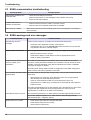
SUNA general troubleshooting................................................................................................... 49
SUNA operation troubleshooting................................................................................................ 49
SUNA communication troubleshooting...................................................................................... 50
SUNA warnings and error messages......................................................................................... 50
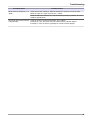
Section 6 General information ....................................................................................................... 53
6.1 Warranty..................................................................................................................................... 53
6.2 Service and support................................................................................................................... 53
6.3 Waste electrical and electronic equipment................................................................................. 53
2
Section 1
Specifications
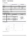
1.1 Mechanical
SUNA with optional wiper
Standard SUNA
Rated depth
100 m
500 m
Weight (in air)
3.1 kg
2.5 kg
Pathlength
10 mm
5 mm
cm3
Displacement
2092
Length
588 mm
Diameter
63 mm
Material
Acetal
Temperature range, operation
0–35 °C
Temperature range, dry storage
-20–50 °C
2084
10 mm
cm3
583 mm
1749
cm3
567 mm
5 mm
1745 cm3
562 mm
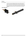
1.1.1 Bulkhead connector
Contact
Standard
Optional (USB/SDI-12)
1
Voltage in 8–18 VDC (15 VDC for sensors with wiper)
2
Ground
3
—
USB 5 V power
4
—
SDI-12
5
RS232 TX
RS232 TX/USB D+
6
RS232 RX
RS232 RX/USB D-
7
—
Analog V out
8
—
Analog current out
MCBH-8-MP
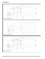
1.1.2 Dimensions
10 mm pathlength without wiper
3
Specifications
10 mm pathlength with wiper
5 mm pathlength without wiper
5 mm pathlength with wiper
4
Specifications
1.2 Electrical
Input
8–18 VDC
Input, sensor with wiper
8–15 VDC
Current draw, operation
~625 mA at 12 V (nominal)
Current draw, supervised low power
(Periodic mode)
< 30 µA
Current draw, processor low power
(Polled mode)
< 3 mA polled
Current draw, standby
(SDI-12 mode)
~20 mA at 12 V
Baud rate
57600 (9600, 19200, 38400, and 115200 available)
Communication interface
RS232 (USB and SDI-12 optional)
Data storage
2 GB (optional)
1.3 Optical
Spectral range
190–370 nm
Light source
UV deuterium lamp (900 hr lifetime)
1.4 Analytical
1.4.1 Nitrate measurement accuracy
Concentration
range
Seawater and fresh water calibrations, 10 mm
pathlength
Seawater and fresh water calibrations, 5 mm
pathlength
Sensor-specific
Class-based
Sensor-specific
Class-based
Best accuracy
2 µM (0.028 mgN/L)
2.5 µM (0.035 mgN/L)
4 µM (0.056 mgN/L)
4.5 µM (0.063 mgN/L)
up to 1000 µM
(14 mgN/L)
10%
20%
10%
20%
up to 2000 µM
(28 mgN/L)
15%
25%
15%
25%
up to 3000 µM
(42 mgN/L)
20%
30%
15%
25%
up to 4000 µM
(0.056 mgN/L)
25%
•
•
•
The specified accuracy is best accuracy or a percentage, whichever is more.
A sensor-specific calibration uses extinction coefficients from the sensor itself.
A class-based calibration uses extinction coefficients that are the average of many
sensors.
5
Specifications
1.4.2 Nitrate measurement precision
Processing configuration
Seawater or fresh water with T-S
correction
Seawater (0–40 psu)
Short-term precision (3 sigma) and limit of detection
0.3 µM (0.004 mgN/L)
2.4 µM (0.034 mgN/L)
< 0.3 µM (< 0.004 mgN/L)
< 1.0 µM (< 0.014 mgN/L)
1.0 µM (0.014 mgN/L)
8.0 µM (0.112 mgN/L)
Change ("drift") per hour of lamp time
Limit of quantification
6
Section 2
Operation
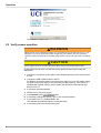
2.1 Install software
The Universal Coastal Interface (UCI) software communicates with a number of sensors.
Refer to the sea-birdcoastal.com website for the current list of sensors that use this
software.
1. Get the software from the sea-birdcoastal.com website or the manufacturer-supplied
CD.
2. Double-click on the file with ".exe" appended to the name.
3. Push Run in the new window.
The setup wizard starts.
4. Push Next.
5. Push Agree in the next window to agree with the terms of the software.
6. Install the software at the default location or push Browse to go to another location to
install the software.
7. Push Next.
8. Put a check in the boxes next to the "Install USB-Serial Driver and "Show Readme."
9. Push Finish.
7
Operation
The software is ready to use.
2.2 Verify sensor operation
WARNING
Nitrate sensors use an ultraviolet (UV) light. Do not look directly at a UV light when it is on. It can
damage the eyes. Keep products that have UV light away from children, pets, and other living
organisms. Wear polycarbonate UV-resistant safety glasses to protect the eyes when a UV light is
on.
CAUTION
Do not supply more than 15 VDC to the sensor. More than 15 VDC will damage the wiper.
Do the steps below to make sure that the sensor operates before further setup and
deployment.
1. Connect the connectors on the cable to the bulkhead connector on the sensor and to
the PC.
2. Connect the USB or RS232 cable to the PC.
For RS232: connect the power connectors on the cable to a 8–15 VDC power supply.
For USB: a DC power supply is only necessary for data collection. If the sensor is
equipped with internal memory, the file system will show as a USB mass storage
device on the PC.
3. If necessary, start the software.
4. RS232: turn on the power supply.
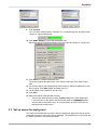
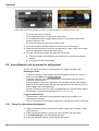
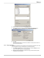
5. Push Connect in the UCI Dashboard area.
6. If necessary, change the "Sensor Type" to the connected sensor.
7. Put a check in the "Try All Baud Rates" box.
The software automatically finds the correct baud rate.
8. If necessary, select the communication port.
8
Operation
9. Push Connect.
The "Connection Mode" shows "Transition" on a yellow background, and then shows
"Setup" on a green background.
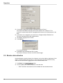
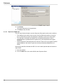
10. Push SUNA Settings in the SUNA Dashboard area.
Make sure that the "Operational Mode" at the top of the new window is "Continuous."
11. Push Start in the SUNA Dashboard area.
The sensor collects data that shows in the Spectra Graph and Time Series Graph
tabs.
12. For sensors that are not equipped with internal memory: Select the View menu, then
Data Logging. Push Start Log to save data to the PC.
13. Let the sensor collect data for a minute or two.
14. Push Stop.
15. Make sure that the collected data is saved.
•
•
Sensors with internal memory: select Transfer Files in the SUNA Dashboard.
Look at the files on the right for the file that was most recently saved.
Sensors without internal memory: Go to the directory on the PC to see the file
that was most recently saved.
2.3 Set up sensor for deployment
The sensor can be attached to a cage or pipe for deployment. Make sure that the sensor
is attached correctly or the sensor may be damaged. The manufacturer recommends that
the sensor operates in a horizontal orientation.
9
Operation
SUNA optical area pointed sideways, and down, to reduce the collection of sediment and bio-fouling.
•
•
•
•
Do not use the wiper as a handle.
Do not attach the sensor to a cage or pipe at the wiper.
Do not attach the sensor so tightly that the sensor is out-of-round. Failure of the
pressure seals can occur.
Do not let the wiper touch any part of a cage or pipe.
1. Use cradle clamps to attach the sensor to a flat surface such as a cage.
2. Make sure that both ends of the sensor are attached to a cage or pipe. Do not leave
one end unattached, such as at the end of a pipe.
3. The user can attach the sensor to a cage with hose clamps:
a. Put several layers of electrical tape around the sensor to protect the pressure
housing.
b. Put clamps over the electrical tape.
2.4 Use software to set up sensor for deployment
The user can deploy the sensor in an autonomous or a logger-controlled mode.
Autonomous modes
•
•
•
Continuous operation—when started, the sensor operates until the user removes
power or pushes Stop in the SUNA Dashboard.
Fixed-time operation—the sensor operates for a user-specified period of time or
number of measurements.
Periodic operation—the sensor operates at user-specified intervals. Data collection
begins at a user-specified date and time and stops when the user removes power or
pushes Stop in the SUNA Dashboard.
Example: a sensor set up at 8:00 with a "Sample Interval" of 2 hours and an offset of
900 seconds (15 minutes) will operate at 10:15, 12:15, 2:15, etc.
Logger-controlled modes
•
•
Polled operation—the sensor communicates through and is controlled by an
RS232 terminal program.
SDI-12—The sensor communicates through and is controlled by an SDI-12 controller.
2.4.1 Set up for autonomous deployment
1. Make sure that the sensor is connected to a power supply and PC (RS232 or USB
cable) and is on.
2. Make sure that the software is open and in communication with the sensor.
3. Push SUNA Settings in the SUNA Dashboard area.
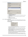
4. Select the "Operational Mode" for the planned deployment.
10
Operation
5. Use the manufacturer-set values for that operation mode or change them as
necessary.
6. If the sensor has an integrated wiper, put a check in the "Integrated Wiper Enabled"
box.
The wiper operates one time data is collected, but no more than once per hour.
7. If the sensor is to be deployed in fresh water but has a calibration for seawater, select
the Advanced tab and put a check in the "Deployed in Fresh Water" box.
8.
9.
10.
11.
Push Upload to save the settings in the sensor.
Push OK to save any changes, or push Cancel to close the window with no changes.
Go to the UCI menu at the top of the software window and select Exit (Ctrl-e).
Exit the software:
•
•
Push No to close the software.
Turn off the sensor, remove from the power supply and attach the protective
dummy connector and lock collar.
Push Yes to close the software and start the sensor. The sensor will collect data
immediately if the user selected "Continuous" or "Fixed-time" or at the userspecified time if "Periodic" was selected.
2.4.2 Set up for SDI-12 deployment
The user can deploy the sensor in a logger-controlled mode with an SDI-12 controller.
1.
2.
3.
4.
Set up the sensor in SDI-12 mode to operate with a controller.
Make sure that the sensor is connected to and in communication with the software.
Push SUNA Settings in the SUNA Dashboard.
At the General tab, select the "SDI 12 Operational Mode."
11
Operation
5. If necessary, change the "Number of Measurements per Frame."
The sensor calculates the average of the value entered. For example, if "5" is
entered, 5 measurements will be averaged and will show as one measurement in the
data.
6. If the sensor is so equipped, put a check in the "Integrated Wiper Enabled" box.
The wiper operates before each measurement.
7. The default "Logging Level" is INFO.
8. Push Upload.
A new window shows.
9. Push Yes to put the SUNA into SDI-12 mode.
The sensor is ready to connect to an SDI-12 data logger.
2.5 Monitor data collection
Use the software to monitor data as it is collected, or to look at it after a deployment, if the
sensor is equipped with internal memory. If the sensor does not have internal memory,
make sure to use the Data Logging tab to save collected data to a PC.
1. Push Start in the SUNA Dashboard area.
2. From the View menu, select the options to see the data:
•
12
Real Time Data—shows the most current data from the selected sensors.
Operation
•
Data Logging—Push Start Log to save the collected data to the PC.
•
Time Series, Spectra, and Total Absorbance graphs.
3. Push Select Sensors to see a list of parameters that can show in the Time Series
tab.
4. Put a check in the box next to any additional parameters so that they will show in the
Time Series graph.
5. Look at the data in the Time Series tab.
•
•
Put a check in the box next to "Time Axis" to push Zoom In and Zoom Out to
change the scale of time.
Put a check in the box next to "Range Axis" to push Zoom In and Zoom Out to
change the scale of the data.
13
Operation
•
•
To move the data in any direction, push the "Ctrl" key on the PC keyboard and
the left button of the mouse pointer at the same time.
To select a specific part of the data to zoom in on, pull the mouse pointer
diagonally (refer to the arrow in the graph below).
2.5.1 Monitor data in spectra graph
The Spectra graph shows both the dark and light data in raw counts.
The dark counts are from thermal noise. The light counts are the measured output minus
the dark counts.
The measured spectrum is always flat below 200 nm, and then has four or five peaks.
The peaks are approximately 25 nm apart in the lower wavelength range and up to 50 nm
apart in the upper range.
1. Put a check in the box next to either or both the "Wavelength Axis" or the "Range
Axis" to enable the Zoom In or Zoom Out options.
The user can change the values for the axis with a check in the box.
2. Push Select Sensors either in the Time Series graph or in the Real Time Display tab
to select the parameters to see on the graph.
3. Push Configure to put a limit on or to remove the limit to the "Time Axis Range."
2.5.2 Monitor data in time series graph
The Time Series graph shows the nitrate concentration and any selected optional values.
Use this graph to replay data that is stored in the sensor.
14
Operation
1. Put a check in the box next to either or both the "Time Axis" or the "Range Axis" to
enable the Zoom In or Zoom Out options.
2. Push Select Sensors either in the Spectra graph or in the Real Time Display tab to
select the parameters to see on the graph.
3. Push Configure to put a limit on or to remove the limit to the "Graph History."
2.5.3 Monitor data in absorbance graph
The Total Absorbance graph shows the calculated absorbance from 210 to 370 nm. This
graph is an alternative to the Spectra graph. The absorbance graph should be flat when a
sample of DI water is collected. The absorbance increases as absorbing species such as
nitrate and bromide are added to samples.
2.6 Get data from sensor
CAUTION
Do data transfers away from harsh environments such as strong electric fields or electrostatic
discharge sources. Electrostatic Discharge (ESD) sources may temporarily disrupt data transfer. If
this occurs, move the sensor away from the ESD source. Turn the power off and then on and
continue operation.
If the sensor is equipped with internal memory, the collected data is saved in the sensor.
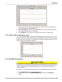
1. Push Transfer Files in the SUNA Dashboard area.
The files saved on the sensor show on the right side of the new File Manager
window.
15
Operation
2. Select one or more files to copy to the PC.
The manufacturer recommends that the user use a USB connection to move the files
because it is much faster.
3. Push the <- arrow to start the move.
The status shows at the bottom of the File Manager window.
4. Open the file on the PC to make sure it has all of the collected data.
16
Section 3
Maintenance
3.1 Sensor maintenance
Although the sensor is built for deployment in severe conditions, it is important to clean
the sensor before each deployment and weekly (if deployed frequently) or monthly to
prevent fouling.
After every deployment:
1.
2.
3.
4.
Attach a clean and lubricated dummy plug and a lock collar to the sensor.
Rinse the sensor with fresh clean water.
Flush the optical area with fresh clean water.
Dry the sensor.
Use a soft towel or blow with air.
5. Put the sensor in the manufacturer-supplied case for transport or storage.
3.2 Maintenance for bulkhead connectors and cables
WARNING
If the user thinks that a sensor has water in the pressure housing: Put on safety glasses and make
sure that the sensor is pointed away from the body. Use the purge port (if the sensor is so
equipped), or very SLOWLY loosen a bulkhead connector to allow the pressure to escape.
NOTICE
Connectors that have corrosion can cause a loss of data and increase the costs for service.
•
•
•
•
•
Connectors that have corrosion can cause irreparable damage to the sensor.
Do not use cleaners that contain petroleum or ketones.
Do not use the cable to lift the sensor. The cable, cable splices, and bulkhead connectors can
be damaged.
Attach cleaned and lubricated dummy connectors to the sensor immediately after each
deployment to prevent the bulkhead connector from damage
Do not connect or disconnect connectors under water.
Examine, clean, and lubricate bulkhead connectors each time they are connected.
Connectors that are not lubricated cause wear and tear on the rubber that seals the
connector contacts.
1. Clean the connector contacts with isopropyl alcohol. Apply as a spray or with a nylon
brush or lint-free swabs or wipes.
2. Flush the contacts with de-ionized or distilled water. Use a wash bottle with a nozzle
to flush inside the sockets.
3. Shake the socket ends and wipe the pins of the connectors to remove water.
4. Examine the sockets and the rubber on the pins to make sure there are no problems.
a. Use a flashlight and magnifying glass.
b. Look for cracks, frayed scores, and delamination of the rubber on the pins and
inside the sockets.
17
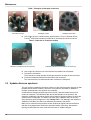
Maintenance
Table 1 Examples of damaged connectors
Corroded connector
Damaged contact
Damaged socket face
5. Use a finger to place a small quantity, approximately 1.5 cm in diameter of Dow
Corning® 4 Electrical Insulating Compound on the socket end of the connector.
Table 2 Lubricant on connector sockets
Lubricant on socket end of the connector
Lubricant pushed into the sockets of the connector
6. Use a finger to push as much of the lubricant as possible into the sockets.
7. Connect the connectors.
There should be a small quantity of lubricant pushed to the sides of the connectors.
8. Clean the unwanted lubricant from the sides of the connectors.
The connectors are now lubricated and the connection is waterproof.
3.3 Update reference spectrum
The user needs to update the reference spectrum of the SUNA at regular intervals so that
the data that the sensor collects is accurate. It may also be necessary to update the
firmware, although that is not required very frequently.
A calibration file contains the data required to convert a spectral measurement into a
nitrate concentration. The calibration data are the wavelengths of the spectrum, the
extinction coefficients of chemical species and a reference spectrum relative to which the
measurement is interpreted. The sensor can store many calibration files, but only the
active file has a green background. Push Transfer Files > File Manager, then select the
Calibration Files tab to see the list of calibration files stored in the sensor.
Make sure to clean the sensor and the sensor windows at regular intervals and before
and after every deployment. Monitor the spectral intensity of the lamp. Although the
intensity will decrease over time, make sure there are no sudden changes.
18
Maintenance
Necessary supplies:
•
•
•
•
•
•
•
•
Power supply
PC with software
Connector cable for sensor–PC–power supply
Clean de-ionized (DI) water
Lint-free tissues
Cotton swabs
Isopropyl alcohol (IPA)
Parafilm® wrap
Notes
•
•
•
•
Use only lint-free tissues, OPTO-WIPES™, or cotton swabs to clean the optical
windows.
Use the software to update the reference spectrum.
Use only clean DI water that has been stored in clean glassware.
Use Parafilm® wrap to capture DI water in the optical area of the sensor. Do not use
cups, a bucket, or a tank to collect a reference sample.
1. Clean the sensor:
a. Flush the sensor and the optical area with clean water to remove debris and
saltwater.
b. Clean the metal parts external to the optical area so that the Parafilm® will seal.
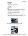
2. If the sensor has a wiper, carefully move it away from the optical area.
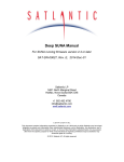
Figure 1 Wiper moved from optical area
3. Cut and stretch a length of approximately 40 cm (16 in.) of Parafilm®.
4. Wind the Parafilm® around the metal near the optical area.
Figure 2 Parafilm® on optical area
19
Maintenance
5. Break a small hole in the top of the Parafilm® and fill the optical area with DI water.
Figure 3 Optical area filled with DI water
6. Supply power to the sensor and use the software to operate the sensor in
"Continuous" mode.
7. Start the sensor and collect 1 minute of data.
8. Record the measurement value.
This is a "dirty" measurement to record the value when there are biofouling and
blockages in the optical area.
9. Stop the sensor.
10. Remove the Parafilm® and drain the water from the optical area.
11. Clean the optical area:
12.
13.
14.
15.
16.
17.
18.
19.
20.
a. Use DI water or IPA and cotton swabs and lint-free tissues to clean the windows.
b. Use vinegar to clean debris such as barnacles. Be careful that the windows do
not get scratches.
Flush the optical area with DI water to remove any remaining IPA or vinegar.
Wind Parafilm® around the metal near the optical area.
Break a small hole in the top of the Parafilm® and fill the optical area with fresh DI
water.
Supply power to the sensor and use the software to operate the sensor in
"Continuous" mode.
Start the sensor and collect 1 minute of data.
Record the measurement value.
This measurement shows any sensor "drift" or change in the lamp output.
Stop the sensor.
Remove the Parafilm® and drain the water from the optical area.
Flush the optical area with DI water.
21. Wind Parafilm® around the metal near the optical area.
22. Break a small hole in the top of the Parafilm® and fill the optical area with fresh DI
water.
23. Supply power to the sensor and use the software to operate the sensor in
"Continuous" mode.
24. Start the sensor and collect 1 minute of data.
25. Record the measurement value.
26. Use the software to update the reference spectrum.
a. Go to the Sensor menu, then select Update Calibration.
20
Maintenance
b. Do the steps in the Calibration Wizard to update the reference spectrum.
27. If the measurement is ±2 µM (0.028 mgN/L) from the manufacturer-supplied
reference (±5 µM [0.056 mgN/L] for a 5 mm pathlength sensor), the sensor is within
the specification.
If the measurement is not within these specifications, do this procedure from step
9 until the measurement is within specification.
3.4 Update firmware
At regular intervals, make sure that the current firmware is installed in the SUNA. Go to
the seabird-coastal.com web site to get the current firmware for the sensor.
1. Save the firmware to the PC.
The firmware is an ".sfw" file.
2. Make sure that the sensor is connected to the PC and a power supply.
3. Push Connect.
4. Go to the Sensor menu, then select SUNA, then Advanced, then Upload Firmware
File.
5. Push Browse to find the firmware file that is saved on the PC.
6. Push Open.
7. Push Upload.
It takes approximately 2 minutes for the software to complete the upload.
8. The firmware is updated.
The software disconnects the sensor.
21
Maintenance
22
Section 4
Reference
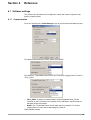
4.1 Software settings
This section has information about configuration values and modes of operation that
apply to all deployments.
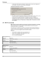
4.1.1 Communication
Go to the Telemetry tab in SUNA Settings to set up communication and data file types.
The default serial baud rate is 57600. Others are available.
The default for "Transmitted Frame Format" and "Instrument Logging Frame Format" is
"FULL_ASCII."
•
•
FULL_ASCII—Contains all collected data in comma-separated fields. The file
extension is .csv. The frame size is typically 1600–1800 bytes. Use this format so
that data can be reprocessed.
NONE—For "Transmitted Frame Format" data output is turned off. For "Sensor
Logging Frame Format" sensor data storage is turned off.
Other available formats:
23
Reference
•
•
•
•
•
•
FULL_BINARY—Contains all collected data. The file extension is .bin. The frame
size is 632 bytes. Use this format so that data can be reprocessed.
REDUCED_BINARY—Contains data from part of the spectrum and data from some
auxiliary sensors. The file extension is .bin.The frame size is 144 bytes. Use this
format so that seawater data can be reprocessed.
CONCENTRATION ASCII—Contains a time-stamp, nitrate concentration,
absorbance at 254 and 300 nm and Root Mean Square Error (RMSE) to measure the
quality of the data. The file extension is .csv.
APF—Used for APEX floats. Contains the user-selected parts of the spectrum and
other auxiliary sensors. The frame size is typically 300–400 bytes.
The user can set the "Transmitted Frame Format" to "NONE" to turn off data output.
This increases the rate at which data is collected, and uses 10–30% less power.
The user can set the "Instrument Logging Frame Format" to NONE to turn off internal
data collection.
The default "Log File Creation Method" is "By File Size." Others are available.
•
•
By File Size—The software makes a new file when the data file in use gets to the
user-selected maximum size. The file name starts with "C" ("Continuous" file).
By Sample Event—The software makes a new file when data collection starts for the
first time after the power has been turned off, then on. The manufacturer
recommends that the user select this for testing only. Use of this setting can result in
so many stored files that the sensor operates slowly or incorrectly. The file name
starts with "A" ("Acquisition" file). Daily—All data that is collected during a calendar
day is put into a single file. This file name is a seven-digit number that is the year and
the day of the year, for example, D2015142.csv. The file name starts with "D" ("Datestamped" file).
The default "Maximum File Size" is 2 MB when the "Mode of Operation" is set to
"Continuous." It is user-selected from 1–65 MB. The "Daily" and "Sample Event" files
contain all of the data that is collected during the day or during one cycle of operation.
4.1.1.1
File types
The sensor uses three types of files:
•
•
•
Data—either ASCII (.csv), or binary (.bin).
Calibration—reference spectrum updates from the manufacturer (.cal).
Log—information about the sensor (.log)
Table 3 Information in data files
Column
Data type
Full ASCII
Full Binary
1
Date, yyyy-mm-dd
2
Header and serial number
N/A
3
Date, year and day-of-year
AI7
BS 4
4
Time, hours of day
AF
BD 8
24
Reference
Table 3 Information in data files (continued)
5
Nitrate concentration, µM
AF
BF 4
6
Nitrogen in nitrate, mgN/L
AF
BF 4
7
Absorbance, 254 nm
AF
BF 4
8
Absorbance, 350 nm
AF
BF 4
9
Bromide trace, mg/L
AF
BF 4
10
Spectrum average
AI
BU 2
11
Dark value used for fit
AI
BU 2
12
Integration time factor
AI
BU 1
13–268
Spectrum channels
256 x AI
256 x BU 2
269
Internal temperature, °C
AF
BF 4
270
Spectrometer temperature, °C
AF
BF 4
271
Lamp temperature, °C
AF
BF 4
272
Cumulative lamp on-time, secs
AI
BU 4
273
Relative humidity, %
AF
BF 4
274
Main voltage, V
AF
BF 4
275
Lamp voltage, V
AF
BF 4
276
Internal voltage, V
AF
BF 4
277
Main current, mA
AF
BF 4
278
Fit aux 1
AF
BF 4
279
Fit aux 2
AF
BF 4
280
Fit base 1
AF
BF 4
281
Fit base 2
AF
BF 4
282
Fit RMSE
AF
BF 4
283
if CTD: Time, secs
AI
BU 4
284
if CTD: Salinity, PSU
AF
BF 4
285
if CTD: Temperature, °C
AF
BF 4
286
if CTD: Pressure, dBar
AF
BF 4
287
Check sum
AI
BU 1
Terminator
<CR><LF>
—
25
Reference
4.1.2 Continuous and fixed-time operation
The sensor must regularly collect a dark spectrum measurement so that it has a baseline
correction for changes in time or "drift" in the output of the spectrometer.
The user can set up the sensor to collect a dark spectrum measurement on a time-based
or measurement-based schedule. A typical setup is a 1-second dark spectrum
measurement for each 20–30 seconds (20–30 measurements) of the light spectrum.
4.1.3 Periodic operation
Use the software to see and change the settings for this mode of operation.
26
Reference
1. Select a "Sample Interval" from the drop-down menu.
2. Look at the "Offset" value. An offset value of 300 (5 min) changes the start time by
five minutes, for example, from 06:00 to 06:05.
3. The "Light Frames" value is 0–255.
Data is collected for either a user-selected quantity of time or a user-selected number of
measurements.
Note: "Periodic" and "Autonomous" are both terms for the same mode of operation.
4.1.4 Polled operation
Use the software to see and change the settings for this mode of operation.
Use the commands below to communicate with the sensor in RS232.
Command
Result
Start
Start continuous data collection.
$
Stops the sensor data collection.
Measure N The sensor gets "n" light data frames. If "n" is zero, the sensor gets one dark data frame.
Timed N
The sensor gets light data frames for "n" seconds.
CTD
The sensor sends CTD data to be corrected for temperature and salinity. The sensor must be set up to do the
correction and to process it.
Status
Print the status of the sensor.
Sleep
The sensor goes to low power standby mode.
Data files are saved in "FULL_ASCII."
Note: "Polled" and "Logger-controlled" are both terms for the same mode of operation.
27
Reference
4.1.5 Other general settings
Sample Averaging, Deployment Characteristics—The average of the number of frames
selected. The higher the value, the more time it takes to make a measurement. The
"Estimated Frame Rate" is directly related to the "Number of Measurements per Frame."
The manufacturer recommends a value of 10–15 as the "Number of Measurements per
Frame" to increase precision in a stable water sample. Use a lower value for unstable
water samples.
Wiper Settings—If the sensor is equipped with a wiper, the user can put a check in this
box so that the wiper will operate before each measurement.
SUNA Messages—The sensor gives information about the sensor operation and
collected data. The default is "Info."
•
•
"Error" gives the least information.
"Debug" and "Trace" give the most information and are used only for troubleshooting.
Set the "Maximum Log File Size" to "0" to turn off the messages.
Options to monitor data
The user can select additional parameters to look at from the Real Time Display tab in the
main window of the software. Push Select Sensors and put a check in the box next to
the parameter to measure.
4.1.6 Compare reference spectrum files
Compare the change between two reference spectrum files. The amount of change is
related to the time interval between the updates and the amount of lamp use during that
time.
Note that this procedure is done automatically by the software when the user updates the
reference spectrum for the sensor. Refer to Update reference spectrum on page 18 for
more information.
1. Find the two files to compare:
28
Reference
a.
b.
c.
d.
e.
f.
g.
Push Transfer Files in the SUNA Dashboard area.
Select the Calibration Files tab.
Select the first file under Instrument filesystem.
Select the directory in the Local filesystem to save the file in.
Push the <-- to move the first file.
Do steps d and e to move the second file.
Push Close.
Note that the date of the files changes to the current date.
2. Select the Data > SUNA > Compare Calibration menu
3. Push Browse to find to the first reference, or calibration, file on the PC to compare.
4. Push Browse to find to the second reference, or calibration, file on the PC to
compare.
5. Push Compare.
A typical update interval of 3–6 months with no more than 100 hours of lamp use
should cause a change of no more than 10% in the 215–240 nm interval.
Below 215 nm, larger relative changes are normal.
Above 240 nm, the change is smaller than at the 215–240 nm range.
If there is a large change, do several reference updates 12–24 hours apart to monitor
the stability of the reference spectrum.
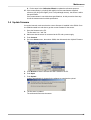
4.1.7 Data acquisition monitor
The software monitors the data collected by the sensor and shows any errors in this
window. The error counters are reset each time the sensor starts a new data collection
file. All information is transmitted during data collection, in real-time.
To see this tab, go to the View menu and select Acquisition Monitor.
29
Reference
•
•
•
•
•
Frame Id—the unique frame number.
Read—The number of frames accepted.
Errors—The number of frames discarded.
Checksum Errors—There may be a problem with the data that is transmitted.
Examine the cabling and connectors. If the value in such is frame is wrong, it is
discarded. If the collected data is saved to the internal memory of the sensor, that
data is correct and can be copied to the PC at a later time.
Counter, Status, and Fitting Errors—always zero.
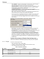
4.1.8 Files necessary to process data
Go to the Data menu to select how data is processed. The HydroCAT can only replay
data.
•
•
•
Use Convert Raw Data to change binary files into ASCII files.
Use Replay Logged Data to show a graph of saved data.
Use Reprocess Data to apply a different reference value or change the settings to
process the data.
The SUNA uses the three files below to process data:
1. The .xml package file that is stored in C:\users\%username%\AppData\Roaming\SeaBird-Coastal\UCI 1.0\SUNA_%SN%.xml.
2. The raw data file to process.
3. The reference spectrum file (optional for Replay Logged Data).
4.1.8.1
Convert raw data
Use the Convert Raw Data option to change binary data to ASCII.
1. Go to the Data menu, then SUNA, then Convert Raw Data.
2. Find the "Instrument Package File" that is stored on the PC.
3. Put a check in the boxes next to the parameters to convert from binary to ASCII.
30
Reference
4. Select the data file to process in the Raw Data Files area.
5. If necessary, change the "Output Directory" in the Converted Data Files area.
Push Options to look at the settings to convert files.
6. Push OK.
The converted file shows in a new tab in the software. It is also saved on the PC in
the directory selected above.
4.1.8.2
Replay logged data
Use Replay Logged Data to look at graphs of the selected data. Data shows in the Time
Series, the Spectra, and the Total Absorbance (if selected) graph tabs.
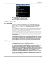
1. Push Replay Logged Data in the SUNA Dashboard, or go to the Data menu, then
SUNA, then Replay Logged Data.
2. Make sure that the package file, the data file to replay, and the reference spectra
("calibration") files are selected.
31
Reference
3. Push Finish.
The saved data shows in the graph tabs.
4. Push Stop to stop the data.
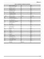
4.1.8.3
Reprocess SUNA data
The user may find that it helps to use the Reprocess Data option under some conditions.
•
•
•
The settings for the sensor were incorrect. Use the Reprocess option to correct for
this, such as when a sensor was deployed in seawater, but set up for fresh water.
The data that is collected has changed over an extended deployment. Data is
processed with an updated reference spectrum file, and compared to the original
reference.
Water temperature and salinity data are collected. These can be put together with the
spectral data from the sensor to get more accurate nitrate data (Sakamoto et al.
2009).
Note that the data files collected with SDI-12 do not contain spectral data and cannot be
reprocessed.
1. Start the software.
2. Go to the Data menu, then select SUNA, then Reprocess Data.
32
Reference
The Reprocessing Dashboard shows.
3. Push Browse to find the package file, the reference file, and the data file required to
reprocess the data.
4. "Processing Settings" are set by the manufacturer and usually do not need to be
changed.
5. Push Process Selected File(s).
The software starts to reprocess the data.
4.1.8.3.1 Nitrate reprocessing details
Settings in "Processing Settings" and the "Temperature & Salinity Correction" areas do
not show until selected by the user. The user can change these settings as necessary to
get better quality data.
Processing settings
•
•
•
•
The default "Enable Raw Data Checksum Validation" is on, with a check in the box. If
it is turned off, raw data can be processed even when the checksum values have
changed after data is collected.
The default "Fitting Range" is 216.5–240 nm. If the wavelength is shorter, seawater
typically causes extinction, and a poor signal-to-noise ratio. If the wavelength is
longer non-characterized materials can be absorbed, which causes a bias in the
processed concentrations.
The default "Max Absorbance Threshold" is 1.3. The precision of the measured
absorbance starts to decline at this value. At 2.5 absorbance units, the precision is at
the "noise floor." The precision of the processed data is better when the low-quality
parts of the "fitting range" are not processed.
The default Seawater Calibration has no check in the box at "Deployed in Fresh
Water." Put a check in this box if the sensor was calibrated for seawater but deployed
33
Reference
in fresh water. Data that was collected in seawater with a check in the "Deployed in
Fresh Water" box gives incorrect nitrate concentrations.
Temperature and salinity correction
•
•
The default "Activate Temperature & Salinity Correction" has no check in the box. Put
a check in this box to add temperature and salinity correction information.
"Temperature and Salinity Correction" is available if the sensor is calibrated for
seawater, and if there is temperature and salinity data available in an ASCII format of
"YYYY-MM-DD hh:mm:ss, Temperature (c), Salinity (PSU)." Push Browse to find the
file to process.
4.2 SDI-12 commands
Note: "Polled" and "Logger-controlled" are both terms for the same mode of operation. The sensor
supports all basic SDI-12 commands. Refer to the SDI-12 specification at www.sdi-12.org for details
of the command protocol. For any command not described below, the sensor will respond
according to the SDI-12 v1.3 specification.
The manufacturer-set address of the SDI-12 is numerical value 48 (ASCII character 0).
The SDI controller uses this address to interface with the sensor in an SDI-12 mode of
operation. The user can change this value in the SDI controller.
Definitions:
•
•
•
•
"a" is the SDI-12 address of the sensor (default is "0")
<CRC> is the 3-character Cyclic Redundancy Check
<CR> is a Carriage Return character
<LF> is a Line Feed character
Acknowledge Active (a!)
Response
a<CR><LF>
Purpose
verifies the SDI-12 address
Example
address = 0
SDI recorder sends 0!
sensor sends 0<CR><LF>
Address query (?!)
Response
a<CR><LF>
Purpose
shows the SDI-12 address
Example
address = a
SDI recorder sends ?!
sensor sends a<CR><LF>
34
Reference
Change address (aAb!)
Response
b<CR><LF>
Purpose
changes SDI-12 address to "b". The default address is 0.
Example
address = 0
SDI recorder sends 0A1!
sensor sends 1<CR><LF>
address now = 1
Verify (V!)
Response
attn<CR><LF>
Purpose
The sensor always responds with a0000<CR><LF> . No diagnostic information is supported.
Send identification (aI!) ("a, capital I, !)
Response
allccccccccmmmmmmvvvxxxxxxxxxx<CR><LF>
a = sensor address
Il (lowercase "L") = 2-character SDI-12 version. For example, "13" for version 1.3
cccccccc = 8-character manufacturer identification. For example, "SATLANTC"
mmmmmm = 6-character sensor model. For example, "SUNA"
vvv = 3-character sensor version. For example, "v2"
xxxxxxxxxxxxx = up to 13-character optional field. Format: F<MAJOR>.<MINOR>.<PATCH>
Used for firmware by the manufacturer.
Example
013SATLANTC SUNA v2 0002F2.1.2<CR><LF>
Start Measurement (aM!)
Start Measurement and Request CRC (aMC!)
Start Concurrent Measurement (aC!)
Start Concurrent Measurement and Request CRC (aCC!)
Response
atttn<CR><LF>
atttnn<CR><LF>
Purpose
starts a measurement.
starts a concurrent measurement.
Notes
a = address = (0–9)
ttt = measurement time in seconds. The sensor typically responds in less than 30 seconds.
n or nn. The number of measurement values the sensor makes and returns after subsequent Send
Data commands. Value = 4.
Example
00104<CR><LF> measurement
001004<CR><LF> concurrent measurement
The sensor reports that 10 seconds are required to do the measurement. Typically it will complete
sooner and send a service request to the controller.
In subsequent data commands, the four values are—
nitrate concentration µM
nitrogen in nitrate concentration mgN/L
light spectrum average
dark spectrum average
35
Reference
Additional Measurement (aM1!)
Additional Measurement and Request CRC (aMC1!)
Additional Concurrent Measurement (aC1!)
Additional Concurrent Measurement and Request CRC (aCC1!)
Response
atttn<CR><LF>
atttnn<CR><LF>
Purpose
starts a measurement.
starts a concurrent measurement.
Notes
a = address = (0–9)
ttt = measurement time in seconds. The sensor typically responds in less than 30 seconds.
n or nn. The number of measurement values the sensor makes and returns after subsequent Send
Data commands. Value = 7.
Example
00067<CR><LF> measurement
000607<CR><LF> concurrent measurement
where 00067 is the address (0), the measurement time (006), and the number of measurements (7).
Example output from the controller:
00M1!
0D0!
00067 <CR><LF>
0+22.7+22.5+141779+46.8<CR><LF>
0D1!
0+12.0+5.0+14.0<CR><LF>
Example output from the controller for the seven values—
Example output values in parentheses:
lamp temperature, °C (22.7)
spectrometer temperature, °C (22.5)
lamp time, seconds (141779)
relative humidity, % (46.8)
internal voltage, V (12.0)
regulated voltage, V (5.0)
supplied voltage, V (14.0)
Additional Measurements (aM2!)
Additional Measurements and Request CRC (aMC2!)
Additional Concurrent Measurement (aC2!)
Additional Concurrent Measurement and Request CRC (aCC2!)
Response
atttn<CR><LF>
atttnn<CR><LF>
Purpose
starts a measurement.
starts a concurrent measurement.
Notes
ttt = measurement time in seconds. The sensor typically responds in less than 30 seconds.
n or nn. The number of measurement values the sensor makes and returns after subsequent Send
Data commands. Value = 7.
Example
36
00099<CR><LF> measurement
000913<CR><LF> concurrent measurement
Reference
Example output from the controller:
00M2!
0D0!
00099 <CR><LF>
0+3.26+0.0457+15501+721<CR><LF>
0D1!
0+2015033+20.57608<CR><LF>
0D2!
0+0.132+0.0672+0<CR><LF>
Example output from the output for the nine (or 13 for concurrent) values—
Example output values in parentheses:
nitrate concentration, µM (3.26)
nitrogen in nitrate concentration, mgN/L (0.0457)
light spectrum average (15501)
dark spectrum average (721)
measurement date (2015033)
measurement time (20.57608)
absorbance at 254 nm (0.132)
absorbance at 350 nm (0.672)
bromide trace (0)
lamp temperature, °C (concurrent measurement only)
spectrometer temperature, °C (concurrent measurement only)
relative humidity, % (concurrent measurement only)
rmse of nitrate processing (concurrent measurement only)
Additional Measurements (aM3–aM9!)
Additional Measurements and Request CRC (aMC3!–aMC9!)
Additional Concurrent Measurement (aC3!–aC9!)
Additional Concurrent Measurement and Request CRC (aCC3!–aCC9!)
Response
atttn<CR><LF>
atttnn<CR><LF>
Purpose
starts a measurement.
starts a concurrent measurement.
Notes
The sensor supports 2 additional measurements.
ttt = 000
n=0
nn = 00
"Send Data" commands that come after the aM! or aMC! commands:
Send Data (aD0!–aD9!)
Response
a<values><CR><LF>
a<values><CRC><CR><LF>
Purpose
sends data to the SDI controller after a measurement or verification command. The response depends
on the previous measurement command.
Note
after the M! or C! command the sensor responds with nitrate concentration in two units, and the light
and dark spectrum average.
Example
0+1039.040+14.8434+22799+671<CR><LF>
Note
after the MC! or CC! command the sensor responds the same as M! or C! but with a CRC value
attached.
Example
0+1038.188+14.8350+22683+672NtW<CR><LF>
Note
after the MC! or CC! command the sensor responds to the aD0! command temperature in two units,
lamp time, and humidity.
37
Reference
Example
0+33.188+23.500+3356+23.2AsF<CR><LF>
Note
The sensor responds to the aD1! command with three voltage units.
Example
0+11.92+5.43+13.68<CR><LF>
after the MC1! command the sensor responds as in the M!! command, but with a CRC value attached.
Example
0+33.813+23.500+3356+23.2AsF<CR><LF>
followed by: 0+11.92+5.43+13.62EyF<CR><LF>
The response to the aC1!, aCC1!, aM2!, aMC2!, aC2!, aCC2! commands is similar.
Continuous Measurement (aR0!–aR9!)
Continuous Measurement and Request CRC (aRC0!–aRC9!)
Response
a<values><CR><LF> or a<values><CRC><CR><LF>
note
the Continuous Measurement command is not supported due to the limited life of the lamp. The sensor
reports a0<CR><LF> or a0<CRC><CR><LF>
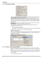
4.3 Terminal program
The user can communicate with the sensor through the manufacturer-supplied software,
or by use of a terminal program through the serial port on a PC. Examples of terminal
programs include Putty, Tera Term, and Bray's Terminal.
When power is supplied to the sensor, the sensor goes into a low-power "standby" mode.
Any activity on the input line puts the sensor to the "SUNA>" command interface within
three seconds. The sensor returns to low-power standby after a user-selected period of
time with no communication.
1. Connect the serial cable to the sensor and the PC.
2. Connect the serial cable to an 8–15 VDC, 1 A minimum, power supply.
3. Start a terminal program.
a. Set up the communication values if necessary: 8 bit, no parity, 1 stop bit, no flow
control.
b. Go to Setup, then Serial Port.
c. If necessary, change the baud rate to 57600. Push OK.
38
Reference
4. Turn on the power supply.
5. Send one or more "$" commands to the sensor to see a prompt at the command line.
The sensor shows "SUNA>" when it is ready to accept commands.
6. Type "get opermode" to see the current mode of operation for the sensor.
The default value is Fixed Time. It shows as "fixedtime." Refer to Data collection
setup values on page 39 for other values for modes of operation.
Table 4 Status commands
Description
Command
Selftest
Result
selftest
Makes sure the sensor operates correctly, does measurements, and
sends those measurements as the last line of output.
$Ok—the sensor operates correctly.
!—A sensor component did not operate correctly.
$Error—A sensor component did not pass the test.
Used lamp time
get lamptime
The total time the lamp has operated, in seconds.
Wiper test
special swipewiper
The wiper operates one time.
Current configuration
get config
The sensor shows the current setup configuration.
Get mode of operation
get opermode
The sensor shows the current mode of operation.
Set mode of operation
set opermode
Changes the mode of operation
7. To change the mode of operation to SDI-12:
a. Make sure that the sensor is so equipped. Type "getopermodesdi12brd"
The response is "available." If the response is "missing", the sensor is not
equipped with SDI-12.
b. Type "set opermode sdi12" to change the mode of operation to SDI-12.
c. Type "get opermode" to make sure that the sensor is in SDI-12 mode.
8. Use the SDI-12 controller to communicate with the sensor when it is in SDI-12 mode.
4.3.1 Input-output configuration values
Parameter
Possible values
Default value
Short name
Baud rate
9600, 19200, 38400, 57600, 115200
57600
baudrate
Message level
Error, Warn, Info, Debug
Info
msglevel
Message file size (MB)
0–65
2
msgfsize
Data file size (MB)
1–65
5
datfsize
Log file type
acquisition, continuous, daily
acquisition
logftype
Acquisition file duration (min)
0–1440
60
afiledur
Data wavelength, low (nm)
210–350
217
wdat_low
Data wavelength, high (nm)
210–350
250
wdat_hgh
4.3.2 Data collection setup values
Parameter
Possible values
Default value
Short name
Operation mode
continuous, fixedtime, periodic, polled, SDI12
fixedtime
opermode
Operation control
duration, samples
samples
operctrl
39
Reference
Countdown (sec)
0–3600
3
countdwn
Fixed time duration (sec)
1–1000000
10
fixddura
Periodic interval
1, 2, 5, 6, 10, 15, 20, 30 (min);
1, 2, 3, 4, 6, 8, 12, 24 (hr)
1 hr
perdival
Periodic offset (sec)
any value
0
perdoffs
Periodic duration (sec)
0–255
10
perddura
Periodic samples (# light frames)
0–255
10
perdsmpl
Polled timeout (sec)
0–65535
10
polltout
Skip sleep at startup
on, off
off
skpsleep
Lamp stability time (ds) ?
0–255
5
stbltime
Lamp switch-off temperature (°C)
* (see note below)
35
lamptoff
Spectrometer integration period (msec)
5–60000
N/A
spintper
Dark averages
1–200
1
drkavers
Light averages
1–200
1
lgtavers
Dark samples
1–65535
1
drksmpls
Light samples
1–65535
10
lgtsmpls
Dark duration (sec)
1–65535
10
drkdurat
Light duration (sec)
1–65535
120
lgtdurat
External device
none, wiper
none
exdevtyp
Ext. dev. pre-run time (sec)
1–120
0
exdevper
Ext. dev. during collection
on, off
off
exdevrun
Ext. dev. minimum interval
1–1440
60
exdvival
Periodic Mode of Operation: When power is supplied to the sensor, the sensor goes to a
low-power standby mode. Any activity on the input line puts the sensor to the "SUNA>"
command interface within three seconds. The sensor returns to low-power standby after a
user-selected period of time with no communication.
Continuous Mode of Operation: Data is collected continuously and autonomously when
power is supplied to the sensor. Data collection stops when the user removes power or
enters a "$" character.
Fixed-time Mode of Operation: data collection occurs for the time set up by the user.
When that time is completed, the sensor enters a low-power standby.
Polled Mode of Operation: the sensor is in low power standby mode until there is activity
on the input line. The sensor initializes in 3–4 seconds, then displays a "CMD?" prompt to
show that is it is ready to receive commands from the controller. The "timeout" value
controls the length of time the sensor is in standby mode before it returns to low power
standby mode.
For best accuracy, regular dark measurements are necessary to compensate for the
change in temperature. Select a dark-to-light data collection rate based on either the
number of samples or the duration.
Note:
The lamp turn-off temperature is 35 °C. The lamp should not operate at temperatures above 35 °C.
When the lamp reaches the turn-off temperature, the sensor overrides the user-configured mode of
operation. The sensor does 5 cycles of 5-light to 5-dark sample collection, then does 1-light to 10dark cycles until the lamp temperature is below the turn-off temperature.
Contact the manufacturer for information to safely change the turn-off temperature.
40
Reference
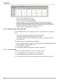
4.3.3 Update firmware
At regular intervals, make sure that the current firmware is installed. Go to the seabirdcoastal.com web site to get the current firmware for the sensor.
1. At regular intervals, make sure that the current firmware is installed. Go to the
seabird-coastal.com web site to get the current firmware for the sensor.Save the
firmware to the PC.
The firmware is an ".sfw" file.
2. Make sure that the sensor is connected to the PC and a power supply.
3. Start a terminal program such as Putty, HyperTerminal®, or Tera Term.
The steps below use Tera Term as an example.
4. Adjust the baud rate to 57600.
5. Turn the power supply on.
6. Type the "$" command to see the "SUNA>" prompt.
7. Type the "upgrade" command then push Enter to see the "SATBLDR>" prompt.
8. Type "w" then push Enter.
9. Go to the File menu, then select Transfer > XMODEM Send....
10. Select the downloaded firmware in the new window and push Open.
The firmware is sent to the sensor.
41
Reference
11. Let the terminal program send the firmware to the sensor.
This process takes a minute or two.
When it is complete, the terminal program shows "$Ok Upload successful."
12. Type "v" then push Enter to make sure that the firmware is valid.
The terminal program shows "$0k Application matches stored CRC-32."
13. Type "a" then push Enter. The SATBLDR starts the new firmware in the sensor.
42
Reference
14. Turn the power to the sensor off, then back on.
The new firmware operates in the sensor.
15. Go to the File menu, then select Disconnect
4.4 Theory of operation
4.4.1 Background
The SUNA is a chemical-free nitrate sensor for fresh, brackish, and salt water. The
sensor is based on the In-Situ Ultraviolet Spectroscopy (ISUS) that was developed at
MBARI (cf. Kenneth S. Johnson, Luke J. Coletti, Deep-Sea Research I, 49, 2002,
1291–1305).
The sensor lights the water sample with its deuterium UV light source and measures this
with its spectrometer. The difference between this measurement and a prior baseline
measurement of pure water is the absorption spectrum.
Absorbance characteristics of natural water components are in the calibration file of the
sensor. The Beer-Lambert law for multiple absorbers makes the relationship between the
total measured absorbance and the concentrations of individual components. Based on
this, the sensor gives a best estimate for the nitrate concentration with multi-variable
linear regression.
If the "Integration Time Adjustment" configuration parameter is set to "On" or "Persistent,"
the sensor makes measurements with a spectrometer integration time that is 20 times as
long as the normal integration time. This increases the signal-to-noise ration in faint light
conditions and lets the sensor operate in optically dense conditions. When the optical
density decreases, the sensor goes back to the normal spectrometer integration time.
4.4.2 Description of nutrient units
Nutrient units express the amount of something, usually moles or mass, relative to the
volume it is in. Many researchers and scientists use micromoles per liter (µM), a unit that
is independent of mass and useful for stoichiometric calculations.
Most fresh water monitoring programs and many researchers use units of milligrams per
liter. This unit is almost always expressed as milligrams of relevant atoms per liter—for
example, milligrams of nitrogen (N) per liter, rather than milligrams of nitrate per liter.
Although nitrate NO3 is the most prevalent form of nitrogen, this unit is frequently used as
a means of easily keeping track of total nitrogen loading. Because milligrams per liter is a
mass-based unit and the mass of N and NO3 are different, this difference is very
important to prevent mistakes. Milligrams per liter is also typically referred to as parts per
million (ppm), the mass of N relative to the mass of water.
The SUNA V2 sensor measures dissolved nitrate and displays units in micromolar (µM)
or milligrams of nitrogen per liter (mg/N/L). The SUNA V2 does not display milligrams of
nitrate per liter (mg/L or mgNO3/L ).
43
Reference
4.4.3 Nitrate concentration
Nitrate processing uses the 217–240 nm wavelength range, which contains
approximately 35 spectrometer channels. The precision of the nitrate concentration is
related to the number of absorbers into which the measured absorbance is decomposed.
High absorbance conditions introduce inaccuracies into the nitrate concentrations.
Channels with an absorbance of more than 1.3 are not included in the processing. If less
than approximately 10 channels remain, the sensor cannot give a nitrate concentration.
The user can increase the absorbance cutoff and get decreased-accuracy nitrate
concentration at higher absorbances.
4.4.4 Description of adaptive sampling
The SUNA V2 has a 256-channel spectrometer that integrates for a specific length of
time, usually 300–500 ms, to maximize the signal while it collects data. When the sensor
does a measurement, the spectrograph collects UV light for the length of the integration
period. In optically dense waters, with high turbidity or CDOM, very little UV light is
transmitted through the water, so the spectrometer "sees" a much lower signal. The
SUNA V2 automatically increases the integration period to compensate for the low light,
so the sensor collects a strong signal in extreme environmental conditions.
4.4.5 Sensor calibration from manufacturer
Sensors come from the manufacturer with a default class-based calibration. Sensors can
have an optional sensor-specific calibration for either fresh water or seawater. The user
can configure a seawater calibration to be deployed in either fresh water or seawater.
The calibration file is stored in the sensor and includes the coefficients to calculate nitrate,
as well as a reference spectrum. It is necessary for the user to update the reference
spectrum as the optical components change over time. The software has a wizard to let
the user update the reference spectrum at regular intervals or as necessary. This
procedure adjusts the "zero" nitrate value based on a sample of pure water (ultra pure,
nano pure, or DI). It is necessary to periodically update the reference spectrum to make
sure that the sensor collects accurate data.
For best performance, send the sensor back to the manufacturer annually for
maintenance.
4.5 Interferences and mitigation
4.5.1 Uncharacterized species in sample
A number of substances in natural water absorb in the UV spectral range where nitrate
absorbs. The spectral signature is usually different from nitrate but certain combinations
of water components may cause a bias in the calculated nitrate concentrations.
If the user thinks there are significant concentrations of interfering species, do a random
spectral and chemical analysis of the water sample to quantify and correct the optical
interference.
4.5.2 Optically dense constituents
The performance of the sensor is compromised in optically dense conditions, which
transmit less light than necessary for the regression analysis. As the optical density
increases, the quality of the measurement (signal-to-noise) decreases. The accuracy and
precision of the nitrate concentration measurements decrease as the quality of the data
decreases. High optical densities are frequently caused by CDOM or turbidity in the water
sample.
4.5.3 Sample temperature
Seawater has a temperature-dependent absorption rate. Make sure to consider this so
that imprecision does not affect the nitrate concentration that is measured. To mitigate
this effect, use the sample temperature and salinity values in the nitrate calculation in the
host software for post-processing. Note that spectra and related temperature and salinity
44
Reference
data is necessary. The temperature-salinity correction comes from MBARI (cf. Carole M.
Sakamoto, Kenneth S. Johnson, and Luke Coletti, Limnol. Oceanogr.: Methods 7, 2009.)
4.5.4 Identification of interfering species
The effect of turbidity and CDOM on the measured nitrate concentration was calculated in
the laboratory.
Turbidity sample
NTU per
mg/L
Absorbance at
225 nm (10 mm)
per mg/L
NO3 change, µM, in
freshwater per mg/L
NO3 change, µM, in
seawater per mg/L
Arizona Road Dust (ARD)
1.25
0.0016
< -0.002 (-2.8 e -5)
0.01 (1.4 e -4)
Kaolin powder
1.5
0.0085
< 0.001 (1.4 e -5)
0.02 (-2.8 e -4)
Titanium dioxide (TiO2)
15.0
0.0090
< 0.001 (1.4 e -5)
< 0.001 (1.4 e -5)
CDOM sample
QSD per mg/L
Absorbance at
particle
225 nm (10 mm) per
mg/L particle
NO3 change, µM, in
seawater per mg/L
particle
NO3 change, µM, in
seawater per mg/L
particle
Pony Lake Fulvic Acid
reference (1R109F)
N/A
0.017
0.4 (5.6 e -3)
0.6 (8.4 e -3)
Suwannee River Fulvic Acid
standard (1S101F)
N/A
0.027
< 0.1 (1.4 e -3)
< 0.1 (1.4 e -3)
Pahokee Peat Humic Acid
reference (1R103H-2)
42
0.003
< 0.01 (1.4 e -4)
< 0.1 (1.4 e -3)
An interfering species causes an incorrect nitrate concentration when its spectral
characteristics are almost the same as nitrate. The RMSE value is the square root of the
mean of the sum of the squared differences between the measured and the fitted
absorbance. The RMSE is a measure of the quality of the fit. Independent measurements
of turbidity and CDOM, and an analysis of the absorption spectrum help the impact
analysis.
4.5.5 Sensor function
The lamp and other optical components in the sensor change with time. This causes
nitrate measurements to change, or "drift." Do regular updates to the reference, or
baseline, spectrum to minimize this change.
The output of the lamp is related to it temperature. The manufacturer recommends that
the user collect the reference (baseline) spectrum in conditions that are almost the same
as a deployment.
45
Reference
4.6 CDOM absorption
Figure 4 Fulvic acid, mg/l. Note that the CDOM spectral shape overlaps with the nitrate processing
region.
The model to calculate nitrate fits for 4 parameters: nitrate, bromide, a temperature
coefficient and a linear baseline correction that accounts for all additional absorbing
species. If the absorption of the sample is high (default cut-off = 1.3 AU), the model can
no longer be used effectively to fit parameters or calculate nitrate concentration. The
SUNA V2 data output is a root mean square error parameter that indicates the quality of
the fit of the models to the absorption curves.
CDOM Absorption Properties
Colored Dissolved Organic Matter (CDOM) is one of the main substance classes that
absorbs in the same UV range as nitrate. (Other significant absorbers are seawater,
bromide, bisulfite, and suspended particles). CDOM is a mixture of many chemicals, and
changes across locations and times, usually depending on its origin. Thus, there is no
universal characterization of the UV absorption of CDOM.
CDOM Impact on SUNA Nitrate Concentration
The UV absorption spectra of CDOM changes across the types of CDOM. Some types of
CDOM are closer in their absorption to nitrate than others. Types of CDOM that absorb
similar to nitrate will cause a larger bias than those that absorb dissimilar. Thus, the
concentration of CDOM alone cannot predict the magnitude of the bias.
Quantification and Correction of CDOM Impact
Under ideal conditions, CDOM would be isolated from all other absorbers, and its
absorbing properties identified in isolation. A more realistic approach is to independently
find the content (nitrate, salinity, CDOM) of a number of water samples (if CDOM is stable
over time), and calculate the CDOM-induced bias on the nitrate concentration.
FDOM: Fluorescent Dissolved Organic Matter is a subset of Colored DOM and can be
used as a proxy for CDOM (if the composition is stable over time). Most FDOM sensors
use a 370 nm excitation source that targets more humic substances, and may not
represent absorption in the nitrate range (~220 nm).
Absorption: The data output of the SUNA V2 is the absorption at 350 nm and 254 nm
(A350 and A254). These wavelengths are outside the nitrate absorption range and can be
used to make an estimate of the impact of CDOM. If absorption is high (>1.3 AU), the
SUNA will not be able to collect adequate light to make a measurement.
46
Reference
RMSE: The root mean square error parameter from the SUNA V2 can be used to make
an estimate of how well the nitrate spectral fit is. This should usually be less than 1E-3. If
it is higher there is spectral shape (likely due to CDOM) that adversely impacts the nitrate
estimate.
Pathlength: SUNA V2 comes in both a 10 mm and a 5 mm pathlength version. Because
absorbance is directly proportional to pathlength, a halved pathlength provides a
tolerance of approximately twice the background absorption.
4.7 Optional equipment
4.7.1 Wiper
The wiper cleans the optical window of biological growth and particulates so that the
quality of the data collected stays constant. The wiper works in all modes of operation of
the sensor. The wiper operates one time before each time that data is collected.
The wiper operates at 90 degrees. Make sure the wiper can operate without any
blockage. Each cycle of the wiper across the optical window takes approximately
15 seconds. There is a minimum required delay of 30 seconds between wiper cycles.
Figure 5 SUNA with wiper
The wiper drive shaft has a mechanism that lets the wiper be moved manually without
damage. Make sure that the wiper is not bent or pushed off of its axis of rotation.
4.7.2 Anti-fouling guard
Use the anti-fouling guard for moored deployments that do not use a pump. The guard is
attached to the sensor by a plastic clamp. The foul guard is made of perforated copper
that goes around the sample volume to prevent biofouling and lets the sample volume
flush. Operate the sensor horizontally and point the sample volume area downward so
that air bubbles and sediment do not collect.
Figure 6 Copper anti-fouling guard
47
Reference
4.7.3 Flow cell
Use the flow cell for moored deployments that require a pump. Attach the flow cell to the
sensor with the manufacturer-supplied plastic clamp. The flow cell seals against the
pressure housing of the sensor so that the water from the pump flows across the optical
path of the sensor. The flow cell has a copper tube on the inlet port and a plastic barbed
fitting on the outlet port that connects to the pump with flexible tubing. Spare parts for the
flow cell include elbow fittings so that the user can adjust the position of the sensor for
deployment.
Figure 7 SUNA flow cell
48
Section 5
Troubleshooting
5.1 SUNA general troubleshooting
WARNING
Nitrate sensors use an ultraviolet (UV) light. Do not look directly at a UV light when it is on. It can damage the eyes. Keep
products that have UV light away from children, pets, and other living organisms. Wear polycarbonate UV-resistant safety
glasses to protect the eyes when a UV light is on.
Possible problem
Sensor does not appear to be on
Possible solution
Check that the cable is connected and the power source is on.
Turn the sensor off for at least 60 seconds. Turn the power on again. If the sensor still
does not appear to be on, use a different cable.
Check that the voltage supplied to the sensor is between 8–15 VDC with at least 1 amp of
current. Check the cable voltage: put the leads of a DMM in DC voltage mode at contacts
1 (+) and 2 (-) of the cable to see if there is voltage. If not, use a different cable.
Check the mode of operation. The sensor may be in an unknown mode. Start a terminal
program, supply power to the sensor, and type "$" then "Enter" three or more times. A
prompt from the sensor shows.
Check the cable for continuity. Refer to the sensor specifications for connector functions.
Check the power consumption. Use a power supply with an accurate digital current
indicator.
•
•
•
current > 500 mA at 12V: sensor is in data collection mode. Put a piece of white
paper into the optical area and make sure that there is a blue spot. If there is not, the
sensor may be in an unknown mode or there is a system failure.
current > 5 mA: sensor is in "standby" mode and gives a result over the RS232 input.
current >100 µA: sensor is not in operation. Contact Customer Support.
5.2 SUNA operation troubleshooting
Possible problem
Possible solution
Self-test fails for internal
humidity
Monitor the sensor and do a sensor self-test at regular intervals. Make sure that the
sensor is not attached to any frame so tightly that the pressure housing is out-of-round.
Self-test fails for low spectrum
average or high dark counts
Clean the optical windows with a low-lint swab or tissue and isopropyl alcohol.
The average value in DI water is within specifications shown below.
•
•
•
Baseline "drift"
Dark spectrum: 500–1000 counts, with a standard deviation of no more than
12 counts.
Maximum light spectrum: no more than 55000, with no more than 60-count standard
deviation.
Average light spectrum: approximately 10000–15000 counts, with ranges to at least
20000 counts. An average value of <10000 may mean that the optical windows are
dirty or stained, or that the lamp is degraded.
Check if the lamp is degraded. Apply drift corrections if the rate is approximately
0.004 mgN/L per hour of lamp "on" time.
Wiper does not operate correctly •
•
•
•
Make sure that there is a check in the box for "Integrated Wiper Enabled" in the
General tab of the Settings tab of the software.
Check the alignment of the wiper brushes and make sure that the wiper is not bent
If the wiper is from another manufacturer, check that the battery contacts are
functional.
Contact Customer Support for further help.
49
Troubleshooting
5.3 SUNA communication troubleshooting
Possible problem
Possible solution
Collected data is different from
transmitted data
•
•
•
Check the clock settings in the sensor.
Make sure that there is no extra averaging or data collection in the setup.
Check the data output settings.
Problems with sensor-tosoftware communication
•
•
Make sure that the sensor-PC cable is connected correctly.
Make sure the current software and firmware are installed.
Self-test fails to complete
Make sure that the sensor has an external power source; external power is necessary to
turn on the lamp.
5.4 SUNA warnings and error messages
Possible problem
Possible solution
Data warnings and error
messages
Contact Customer Support. If possible, have the information listed below:
Negative nitrate concentration
Clean the optical area and check the reference spectrum. Apply a new one if necessary.
•
•
•
•
•
screenshot of the "Application Console" of the software.
"messages.log" file—go to the Transfer Files window and select the Log Files tab.
Copy the file to the PC for Customer Support.
Make sure that the sensor is in water.
Check that the "Deploy in Fresh Water" box has the appropriate check in it.
Check for salinity compensation.
Analysis of nitrate standard shows Check that the nitrate standard concentrations are accurate. Make sure the dilutions
sensor is possibly out of
were done correctly and that the standards are used within 1 week (in the lab) or before
specification
expiration (unopened standards). Verify that the standards were made in comparable
units (mg/L as nitrogen or µMoles).
Check the sensor settings. Make sure that the "Deployed in Fresh Water" setting has a
check in the box if the sensor operates in fresh water.
Poor correlation with field samples Check the sensor for fouling or lamp change ("drift"). Clean the optical windows and do a
(grab samples)
blank check.
•
•
Set the sensor to do a self-test. Check light:dark counts, such as high CDOM or
other absorbers and other data about the sensor.
Check for matrix interferences that can cause measurement errors. Do
measurements for a wider range of constituents an do possible lab matrix spikes to
isolate the cause.
Check the representativeness of the data collection site. If the data from the sensor does
not agree with grab samples but shows good performance, the site may not be
representative of conditions, or the water is not well mixed.
Data collection rate is very slow
Check if the internal memory is on. Data collection starts after approximately 5 seconds.
Check if the "adaptive integration" is on. Data collection starts after approximately
500 milliseconds (20 × "integration period").
Nitrate values are not stable
50
•
•
•
Check that the optical area is not blocked with debris.
Check that the wiper functions correctly.
Clean and dry the optical area.
Troubleshooting
Possible problem
Nitrate value are frequently "-1" or
"NAN"
Possible solution
Check that the lamp intensity is sufficient. Measure the spectrum in DI or tap water.
Maximum output is > 10000. For best case, > 30000.
Check the data: if the maximum is < 1000 and the lamp intensity is sufficient, the water
sample is optically dense.
SELFTEST alert for lamp intensity Check the sensor for high internal humidity. Do a "selftest":
or high humidity
if humidity is > 50%, the sensor may have a leak. Contact Customer Support.
if humdity is > 30%, the sensor is probably ok. Contact Customer Support.
51
Troubleshooting
52
Section 6
General information
Revised editions of this user manual are on the manufacturer's website.
6.1 Warranty
This sensor is warranted against defects in materials and workmanship for one year from
the date of purchase. The warranty is void if the manufacturer finds the sensor was
abused or neglected beyond the normal wear and tear of deployment.
6.2 Service and support
The manufacturer recommends that sensors be sent back to the factory annually to be
cleaned, calibrated, and for standard maintenance.
Refer to the website for FAQs and technical notes, or contact the manufacturer for
support at:
[email protected]
Do the steps below to send a sensor back to the manufacturer.
1. Contact the manufacturer for a Return Merchandise Authorization (RMA).
Note: The manufacturer is not responsible for damage to the sensor during return shipment.
2. Remove all anti-fouling treatment from the sensor before sending it back to the
manufacturer.
Note: The manufacturer will not accept sensors that have been treated with anti-fouling
compounds for service or repair. This includes tri-butyl tin, marine anti-fouling paint, ablative
coatings, etc.
3. Use the sensor's original ruggedized shipping case to send the sensor back to the
manufacturer.
4. Write the RMA number on the outside of the shipping case and on the packing list.
5. Use 3rd-day air to ship the sensor back to the manufacturer. Do not use ground
shipping.
6. The manufacturer will supply all replacement parts and labor and pay to send the
sensor back to the user via 3rd-day air shipping.
6.3 Waste electrical and electronic equipment
Electrical equipment that is marked with this symbol may not be disposed of in European public
disposal systems. In conformity with EU Directive 2002/96/EC, European electrical equipment
users must return old or end-of-life equipment to the manufacturer for disposal at no charge to
the user. To recycle, please contact the manufacturer for instructions on how to return end-oflife equipment, manufacturer-supplied electrical accessories, and auxiliary items for proper
disposal.
53
General information
54
Sea-Bird Coastal
13431 NE 20th Street
Bellevue WA 98005 U.S.A.
sales (425) 401-7653
support (425) 401-7654
[email protected]
www.sea-birdcoastal.com
©
Satlantic, Inc., 2012. All rights reserved. Printed in USA.