1
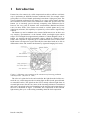
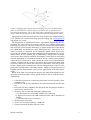
Downloaded from orbit.dtu.dk on: Dec 15, 2015
Development and design of a line imaging spectrometer sampler (LISS) - A user
manual
Jørgensen, Rasmus Nyholm; Rasmussen, P.
Publication date:
2002
Document Version
Publisher final version (usually the publisher pdf)
Link to publication
Citation (APA):
Jørgensen, R. N., & Rasmussen, P. (2002). Development and design of a line imaging spectrometer sampler
(LISS) - A user manual. (Denmark. Forskningscenter Risoe. Risoe-R; No. 1189(EN)).
General rights
Copyright and moral rights for the publications made accessible in the public portal are retained by the authors and/or other copyright owners
and it is a condition of accessing publications that users recognise and abide by the legal requirements associated with these rights.
• Users may download and print one copy of any publication from the public portal for the purpose of private study or research.
• You may not further distribute the material or use it for any profit-making activity or commercial gain
• You may freely distribute the URL identifying the publication in the public portal ?
If you believe that this document breaches copyright please contact us providing details, and we will remove access to the work immediately
and investigate your claim.
Risø-R-1189(EN)
Development and Design of a Line
Imaging Spectrometer Sampler (LISS)
- A User Manual
Rasmus Nyholm Jørgensen1 and Peter Rasmussen2
1)
Plant Nutrition and Soil Fertility Laboratory, Department of Agricultural Sciences, The Royal Veterinary and
Agricultural University
DK-1871 Frederiksberg C (Copenhagen), Denmark
Present address:
Plant Environment Interactions, Plant Research Department, Risø National Laboratory, DK-4000 Roskilde,
Denmark
e-mail: [email protected]
2)
Plant Environment Interactions, Plant Research Department, Risø National Laboratory, DK-4000 Roskilde,
Denmark
February 2002
Risø National Laboratory, Roskilde
Abstract
The objective of this report is to develop and describe the software for a Line
Imaging Spectrometer Sampler (LISS) to perform measurements of spectra
combined with a digital RGB photo of a measurant. Secondly this report should
enable users to perform measurements with the system.
The measuring devices consist of 2 16-bit cooled SBIG ST-6 CCD cameras
each equipped with an Imspector imaging spectrograph for measuring reflectance in the visual and the near infrared range, respectively, a digital camera and
a differential global positioning device (dGPS). The controlling and data collecting tasks are developed as a Graphical User Interfaced (GUI) hosted by Matlab Release 12 from Mathworks. This GUI enables the operator to perform
measurements from all devices simultaneously together with notes specific for
the measurant and store all the data in one Matlab data structure.
The software includes dynamic exposure of the two CCD cameras ensuring
optimal use of 16 bit range under unstable illumination conditions. A routine,
handling dark frame subtraction in a robust manner minimising the effect of hot
pixels is also included.
This report enables a novice user to perform measurements with LISS relatively easy, enabling the user to put the main focus at the analytical phase and
not on the measuring phase.
Keywords: imaging spectrograph, spectrometer, Imspector, Matlab, reflectance
ISBN: 87-550-2706-7; 87-550-2708-3 (Internet)
ISSN: 0106-2840
Print: Pitney Bowes Management Services Denmark, 2002
Contents
PREFACE .......................................................................................................................4
1
INTRODUCTION .................................................................................................5
1.1
2
AIM..................................................................................................................8
MATERIAL AND METHOD...............................................................................9
2.1
MATERIAL .......................................................................................................9
2.1.1 The Hardware Platform..................................................................................9
2.1.2 The Software platform ....................................................................................9
2.1.3 The Measuring Units ......................................................................................9
2.2
METHOD ........................................................................................................10
2.2.1 Green - The normal flow of actions when using LISS...................................11
2.2.2 Red - Flow of action if the setup procedure fails ..........................................12
2.2.3 Grey - Flow of actions when overruling the standard dark frame
interpolation ..........................................................................................................12
2.2.4 Dark blue - Flow of actions when auto sampling are enabled .....................12
2.2.5 Light blue - Free inspection of the measurement performed ........................13
3
LISS SOFTWARE – USER’S MANUAL..........................................................14
3.1
INSTALLING AND SETTING UP MATLAB TO HOST LISS...................................14
3.1.1 The LISS folders............................................................................................14
3.1.2 Placing the LISS folder and setting up Matlab .............................................15
3.1.3 Setting up the PC enabling Matlab to interface the Canon IXUS.................15
3.2
THE LISS USER INTERFACE ..........................................................................15
3.2.1 Sampling data ...............................................................................................16
3.2.2 Time and GPS info........................................................................................17
3.2.3 RGB photo ....................................................................................................17
3.2.4 Control panel................................................................................................17
3.2.5 Camera 1 and Camera 2...............................................................................18
3.3
INITIALISATION OF THE LISS SOFTWARE .......................................................19
3.4
THE SETUP DEFINITION FILE .........................................................................20
3.5
USE OF DARK FRAMES...................................................................................23
3.5.1 How to reduce the dark frame effect to the quality.......................................23
3.5.2 Procedure for using dark frames in LISS......................................................24
3.5.3 Procedure for recording a new darkframe ...................................................25
3.5.4 The structure of the dark frame data file ......................................................25
3.6
MEASURING WITH LISS.................................................................................26
3.6.1 Preparations and decisions prior to measuring............................................26
3.6.2 Single-shot measuring procedure .................................................................26
3.6.3 Multi-shot sampling procedure.....................................................................27
3.7
THE STRUCTURE OF THE MEASURING DATA ...................................................27
3.8
SHUTTING DOWN LISS AND EQUIPMENT .......................................................28
4
REFERENCES ....................................................................................................29
5
APPENDIX – TECHNICAL INFO....................................................................30
5.1
APPENDIX – USING CANON IXUS DIRECTLY FROM MATLAB ........................31
Risø-R-1189(EN)
3
Preface
This manual should enable a novice user to perform measurements with the
Line Imaging Spectrometer Sampler system, LISS, relatively easy. This will
further enable the user to put the main focus on the analytical phase and not on
the measuring phase. Further the reader will be able to build the system from
scratch if needed. But most important, it should inspire the reader to build a new
and better system based on the main principle of the LISS system.
Matlab was selected as the host application for LISS due to its integration of
mathematical computing, visualization, and powerful language in providing a
flexible environment for technical computing. The open architecture makes it
possible to use Matlab and its companion toolboxes to explore data, create algorithms, and create custom tools.
Cand.Agro R. N. Jørgensen has carried out the main idea and the design of the
overall structure of LISS as a part of his Ph.D. project. B.Sc.Hort. P. Rasmussen
has coded and debugged the LISS application.
The Department of Agricultural Science, Agricultural Engineering at The
Royal Veterinary and Agricultural University, Denmark is gratefully acknowledged for lending out their line imaging system full time during the months of
development. We also want to thank the Canon PowerShot Developer Programme for the technical support during the coding of the remote control for the
Canon Digital IXUS camera. Furthermore we are grateful to engineer Johannes
Nyholm Jørgensen for programming the interface file enabling remote control
of the Canon Digital IXUS camera directly from the Matlab command prompt.
Finally, we especially thank all those who read draft copies of the manuscript:
Professor, D.Sc., Ph.D. Niels Erik Nielsen, Research Professor Simon Blackmore, Ph.D. Stud. Lene Krøl Christensen and Associated Professor Henning
Nielsen, The Royal Veterinary and Agricultural University, Department of Agricultural Sciences; Professor D.Sc. Gunnar Gissel Nielsen, Risø National Laboratory, Plant Research Department.
Thursday, 21 February 2002
4
Rasmus N. Jørgensen and Peter Rasmussen
Risø-R-1189(EN)
1
Introduction
Farmers have for centuries by visible inspection been able to tell how well their
crop is performing at different locations within the field. For example a dark
green plant is as a rule of thumb performing better than a light green plant. The
visual evaluation performed by the farmer is to a large extent relative because
the evaluation is based on the color differences within the specific field. The
human eye is extremely good in directly comparing color differences but is
however not very good in absolute color measurements (Hatfield and Pinter
1993). In other words, if the farmer was asked to evaluate plants one by one
without any reference, his capability to separate by color would be significantly
reduced.
The human eye and a standard color camera (RGB camera) are in their own
way imaging "spectrometers" at the limited visible wavelength region which
ranges in wavelength from approximately 400nm to 750nm (Hagman 1996). A
human eye registers the basic tristimulus values, which are relatively broad
bands, and is capable of separating up to 36,000 different colors. Likewise the
RGB camera is designed to register basically the same three bands to be able to
differentiate colors and "imitate" the human eye (Spectral Imaging Ltd. 1999).
Figure 1: Schematic representation of the interaction of incoming radiation
with leaf tissues. (Guyot et al. 1992)
The color of a plant leaf is the end result after the light from the leaf has entered the eye, which integrates the incoming light in three broad spectral bands
as mentioned earlier. The light from the leaf is mainly reflected light from an
external light source like the sun. Some of the incoming radiation is transmitted
and some is absorbed in the leaf depending on the structure and composition of
the leaf as illustrated in Figure 1. Therefore, the composition of the reflected
light entering the eye is a code telling something about the leaf composition.
Risø-R-1189(EN)
5
G
VIS
NIR
B
R
400
500
600
700
800 nm
Figure 2: Schematic illustration of a typical reflection spectrum of a green
plant in the visual (VIS) and near infrared (NIR) range of light when illuminated by the sun. The three graphs (R, G, B) illustrate how an RGB camera integrates light from three broad bands centred red (650 nm), green (530 nm),
and blue (460 nm) simulating the human color vision. (After (Guyot et al. 1992;
Searcy 1989))
However studying Figure 2 it becomes clear that the information contained in
the three broad bands are rather limited when compared to the character of a
leaf reflectance spectra in the visual and near infrared light. One way to obtain
the 'true' reflectance spectrum is to use a spectrophotometer, which is able to
measure both VIS and NIR in very narrow bands. A standard spectrophotometer
is usually only able to measure from a small integrated area at a time. This
means that if one wants to measure the optical spectrum from different spatial
locations of an object, either the measuring instrument or the target has to be
moved or scanned (Spectral Imaging Ltd. 1999). By using a spectrometer, valuable spectral information can be achieved, but the spatial or imaging information is lost. Therefore an imaging spectrometer is needed.
Then, how to realise an imaging spectrometer in practise? Basically, some
kind of component capable of separating different wavelengths (prism, grating
or filter), optics which are used to image spatial features and a detector for
measuring the acquired image. The possibilities are limited considering the present available components and their properties. Technically it is not possible, by
using a standard 2D CCD matrix element (a semiconductor chip with a grid of lightsensitive elements, used for converting light images, as in a television camera, into electrical
signals), to measure simultaneously the 2 -dimensional surface as a matrix plane
(X, Y -plane), the spectrum components with high resolution and the intensity
of each spectral element. However, it is possible to measure the spatial information from a line (with specified length and small but finite width) and the spectral information from equally spaced points on this line. In this way the other
dimension of the CCD array retains its spatial function but the other axis is used
to record the spectrum in each spatial point! The resulting image from the target
is certainly limited, just one narrow line, but still it is much more than just a
point (Spectral Imaging Ltd. 1999).
6
Risø-R-1189(EN)
Figure 3: Imaging spectroscopy (spectral imaging) across a two dimensional
plate. An area detector is able to register position in the X -coordinate axis,
wavelength and intensity. The Y-axis of the plate is measured by acquiring line
images while moving the plate in the Y-direction (Spectral Imaging Ltd. 1997).
Equipment using the latter principles has been designed and manufactured by
VTT, Finland, now commercialised by Spectral Imaging Ltd. (www.specim.fi)
(Hyvarinen et al. 1998).
The Department of Agricultural Sciences, Agricultural Engineering, RVAU,
Denmark, has since 1995 been working with the line imaging spectrometer
technology from Specim. The main focus has been on crop/weed discrimination
and it has been proven that this technology is capable of this kind of discrimination (Bennedsen and Rasmussen 2001; Borregaard 1997; Borregaard et al.
2000). In 1998 R. N. Jørgensen, RVAU Denmark, started a Ph.D. project aiming on the line imaging spectrometer equipment at the Department of Agricultural Sciences, RVAU, with the aim of establishing a nitrogen index in winter
wheat grown under natural conditions. Preliminary results made in corporation
with the Department of Agricultural Sciences, RVAU, indicate great potential
within this area (Nielsen et al. 1999). During this work it was realised that the
software included with the cameras mounted at the two linespectrometer units
could only control one camera unit at the time. Furthermore, it was not possible
to take a digital photo simultaneously with the linespectrometer, since all sampling units used individual controlling software. Finally a GPS position stored
together with the measurements could ease the organisation of the data significantly.
Based on the latter it was decided to design a new application named Line Imaging Spectrometer Sampler (LISS), which should be able to fulfil the following demands:
•
•
•
•
•
•
•
It should be possible to control and collect data from all measuring units
simultaneously
Possible to add specific information for each measurement into the data
file
Data from all units containing the measured data and settings should be
stored in one structured file
Should be able to control the following sampling units:
• 2 CCD cameras ST-6 from SBIG with RS-232 connection
• 1 digital color camera with USB connection which can be interfaced to
Matlab
• 1 GPS unit with RS-232 connection
Windows2000 compatible
Able to run at a laptop with only 1 USB port
Software should be flexible and easy to alter
Risø-R-1189(EN)
7
1.1
Aim
The objective of this report is to develop software for a Line Imaging Spectrometer Sampler (LISS) to perform measurements of spectra combined with a
digital RGB photo of a measurant.
Secondly this report should enable users to perform measurements with the
system.
8
Risø-R-1189(EN)
2
Material and Method
This section will briefly describe the equipment that the LISS software operates
from and the hardware needed to build the whole system. Furthermore the overall mode of action for the whole system is explained with main focus on the
LISS software.
2.1
Material
The hardware and the software from which
the LISS software operates together with the
sampling units are illustrated to the right
and at the front page. The whole system
can be separate into three categories: The
hardware platform, the software platform,
and the measuring units. The content of
these is described below.
2.1.1 The Hardware Platform
The computer hosting the software is a Chicony MP-979 PII-266 with 192 MB Ram.
The laptop has one 9-pin RS-232 port and 2
USB ports. A Xircom USB Port Expansion
is connected to the USB port giving access
to additional 4 RS-232 ports and 1 USB port
extra. The 4 additional RS-232 ports were
setup with serial port id’s from COM3 till
COM6.
2.1.2 The Software platform
The operating system is windows 2000 version 5.0.2195 or higher. The Software platform for the LISS software is Matlab release
12 from Mathworks Inc. equipped with an
Extended Real Time Toolbox version 3.1
from Humusoft enabling Matlab to access
the RS-232 ports.
2.1.3 The Measuring Units
Figure 4: Picture of the LISS
measuring devises. 2 SBIG
CCD cameras equipped with a
NIR and a VIS imspector imaging spectrograph, respectively
and a Canon Digital IXUS located between these.
The sampling units are 2 SBIG ST-6A CCD
Imaging Cameras from Santa Barbara Instrument Group with a resolution of 375 by
242 pixels. The pixel size is 23 x 27 microns and the total CCD array area is 8.6 x
6.5 mm. The readout electronics utilise a
16-bit analogue to digital (A/D) converter
and double correlated sampling to achieve very high sensitivity and photometric
accuracy. Each of these cameras is mounted with an Imspector Line Imaging
Spectrograph for the visual range (model V7) and the Near Infrared range
Risø-R-1189(EN)
9
(model N10), respectively. The orientation of the CCD Imaging Cameras is 242
pixels along the spatial axis and 375 pixels along the spectral axis.
The digital color camera for the documentation photo is a Canon digital IXUS
with 2.1 Mpixels supporting remote control coded in C++ via the USB port.
The GPS receiver is a modified “Nav-Guide +” sending out a $GPGGA
NMEA string at 4800 baud containing the position of the measuring equipment.
The GPS-receiver was modified so the RDS functionality was disabled and the
dGPS string were sent to the Nav-Guide through pin 8 in the RS-232 port. The
dGPS strings were sent to the Nav-Guide from a CSI MBX-3 Beacon dGPS
receiver.
2.2
Method
The flow of actions and decisions normally carried out when using the LISS
software will be described in the following. There is no need to know the actual
user interface of LISS. In fact this section should give a good overview and basis to understanding the overall structure of the LISS software.
Figure 5 is a flow chart illustrating the flow of decisions and actions during a
measuring session with the LISS software. The flow of decisions and actions
needed are grouped in boxes of different colors. The colors represent the following groups:
•
•
•
•
•
Green
Red
Grey
- The normal flow of actions when using LISS
- Flow of actions if the setup procedure fails
- Flow of actions when overruling the standard dark frame interpolation
Dark blue - Flow of actions when auto measuring is enabled
Light blue - Free inspection of the measurement performed
The following text will refer to the boxes in Figure 5 according to their ID’s
placed in the upper part of each box. For example (G1) refers to the first green
box with the content “Start LISS from Matlab”.
10
Risø-R-1189(EN)
G1
G2
G2
Start LISS
from Matlab
G3
G4
Activate the
setup
definitions file
Edit the Setup
definition file
Select path
Yes
G5
Control all enabled
sampling units and
envoke the setting from
the definition file
No
R2
Control equipment
and retry
R1
G6
Display Error
message
The setup was
successful
No
Yes
Gr1
G7
Use standard dark
frames
No
Gr2
Take Sequence of
Dark Frames and
perform linear
regression
Activate Take
Dark Frame
Yes
Gr3
dB4
Save Frame
regression
G8
Is at the end of
sampling sequence
No
Activate Take
Image
Gr4
Save Dark
Frame
regression
Yes
R3
Wait 2 sec
No
dB3
Save
sampling data
G9
dB1
Is CCD
Yes
temperature at set
point
Yes
dB2
Take Image
Is autosampling
enabled
No
No
Yes
G11
Inspect the sample
data before save
No
G13
Save sampling
data
Yes
G12
No
R3
Wait 2 sec
G10
Is CCD
temperature at set
point
Yes
Save the sampling
data
Lb1
Inspect sampling data
No
Figure 5: Flow chart illustrates the decisions and flow of action during a measuring session with the LISS software. The green colored boxes show normal
flow of actions. The red boxes show when something goes wrong. The dark blue
boxes illustrate automated sampling. The light grey boxes show the decisions
needed concerning dark frames, and the light blue box illustrates the flow for
performing manual inspection of data sampling before saving.
2.2.1 Green - The normal flow of actions when using LISS
G1 – The first step is to start the LISS software from the Matlab software,
which serves as host application.
G2 – The next step is to select the path or folder to which the measuring data
files should be saved into.
G3 – When LISS has been started the setup definition file will be copied to the
folder into which the measuring data is saved, if the folder does not already contain any setup file. Hereafter the standard setup definition file is opened to control if any setting needs to be changed.
Risø-R-1189(EN)
11
This step can be overruled, if an existing setup file is already in the selected
path, e.g. if continuing a measurement series.
G4 – When the setup definition file has been saved and closed the setup procedure for the whole system can be initiated manually.
G5 – The setup procedure tests if measuring units, which are enabled in the
setup file, are working. Furthermore, the measuring units and the LISS interface
are set according to setup file.
G6 – Controls if the setup procedure succeeded without any error.
G7 – If no errors occurred during the setup procedure, the user needs to decide
if the standard dark frame interpolation should be used or another dark frame
file should be loaded or if new parameters for the dark frame interpolation must
be estimated. Further the user decides if dark frames are subtracted from the
linespectrometer measurements by setting a radio button on or off.
G8 – Activates the measuring procedure manually.
G9 – Tests if auto sampling is enabled. If not the measuring procedure for one
measurement is started.
G10 – Tests if the CCD temperature is ±1 °C from the pre-set value. If the temperature is valid the measuring procedure is performed.
G11 – User decides if further inspection of the data measured is needed.
G12 – User decides if data should be saved.
G13 – All the measured data is saved in one file as a Matlab structure containing all data of value for later data processing. If autosave is enabled, this is performed automatically after point G10.
2.2.2
Red - Flow of action if the setup procedure fails
R1 – Displays an error message if there is any, explaining the user what went
wrong during the setup procedure.
R2 – The user decides whether to control the measuring devices or alter the
setup definition file.
R3 – Program waits 2 seconds before continuing.
2.2.3 Grey - Flow of actions when overruling the standard dark frame interpolation
Gr1 – Manual activation of the procedure collecting a new set of dark frames
estimating the parameters for a new dark frame estimation.
Gr2 – Procedure collecting dark frames from the CCD imaging cameras after a
sequence of exposure time given in the setup definition file. After collecting the
dark frames linear regressions are performed for each pixel estimating the relationship between exposure and dark noise when no light is entering the well.
Gr3 – User decides if the structure containing the intercept and slope for each
pixel from dark frame regression should be saved.
Gr4 - The structure containing the intercept and slope for each pixel from dark
frame regression is saved as a Matlab structure into a folder containing the sampling data.
2.2.4 Dark blue - Flow of actions when auto sampling are enabled
dB1 – Test if the CCD temperature is ±1 °C from the pre-set value. If the temperature is valid the measuring procedure is performed.
dB2 – Measuring procedure is performed.
dB3 – All the measured data is saved in one file as a Matlab structure containing all data of value for later data processing.
12
Risø-R-1189(EN)
dB4 – Test if the auto sampling procedure is at the end of the measuring sequence given in the setup definition file. If not, the procedure continuous with
dB1, when the time since the last measurement was initiated exceeds the sampling interval given in the setup definition file.
2.2.5 Light blue - Free inspection of the measurement performed
Lb – Allows the user to inspect the data before saving. This can be done by
running various Matlab routines outside the LISS application analysing the data
before deciding whether to save the result or not.
Risø-R-1189(EN)
13
3
LISS software – User’s Manual
This section is build up as a regular user manual, which will enable a novice
operator to use the LISS software. This manual prerequisite the operator is familiar with using Matlab. Further, a minimum knowledge regarding programming terminology of Matlab is needed. The section explains and deals with the
following subjects:
•
•
•
•
•
•
Description of how to install and setting up LISS in order to be able to operate within the Matlab environment.
A detailed description of the LISS user interface with concern to individual
functions and how to operate these.
Point by point explanation of the setup definition file
How to perform the initialisation procedure
Discussing the use of dark frames and how to generate new parameters for
dark interpolation
Finally the actual measuring procedure is described in details
3.1
Installing and setting up Matlab to host LISS
The LISS application does not have any automatic installation procedure.
Therefore the installation must be done manually.
3.1.1 The LISS folders
All routines and data necessary are contained in one main folder, which has
seven subfolders as shown in Figure 6.
Figure 6: Illustration of the folder structure for the LISS application
•
•
•
•
•
•
•
14
The main folder LISS_v4 contains main files for the LISS application plus
the setup definition file and the standard dark frame regression file.
The subfolder Backup_of_initial_LISS_settings contains a backup of the
setup definition file and the standard dark frame regression file.
The interfaces files between Matlab and the Canon Digital IXUS camera are
placed in the Canon_IXUS folder.
The manual is placed in the subfolder LISS Manual in PDF format.
The GPS subfolder is a Matlab interface for picking up a NMEA GPS string
from a RS-232 port and desiccating the $GPGGA string into positioning information.
Subfolder CameraControl and CameraControl_subroutines contain a Matlab interface to the cpu unit controlling the line imaging spectrometers. A
detailed description of the commands is given in the cpu unit manual (Santa
Barbara Instrument Group 1993).
The Temp subfolder is used by the Canon IXUS procedure.
Risø-R-1189(EN)
3.1.2 Placing the LISS folder and setting up Matlab
The LISS main folder and all subfolders must be copied to the Matlab folder on
a computer with Matlab R12 and the extended real time tools box version 3.1
installed. By using the Matlab Path Browser the main folder, shown in Figure 7,
is added to the default path of Matlab.
Figure 7: The LISS folder named LISS_v4, which must be added to the path of
Matlab.
3.1.3 Setting up the PC enabling Matlab to interface the Canon IXUS
After the drivers delivered with the Canon Digital IXUS camera have been installed, a few additional steps are needed to enable the interface from Matlab to
the IXUS drivers.
The first step is to set the registry information necessary from the Matlab
command line that can make Windows call to launch the IXUS drivers. In the
Current Directory bar set the path to C:\matlab\Liss_v4\Canon_IXUS. Then
type !RUNDLL32.EXE PSDKREG.DLL Install in the command window.
For further information on how to control the Canon Digital IXUS camera directly from Matlab see section 5.1 on page 31.
When the settings described above have been done the LISS application can
be executed be typing liss in the Matlab command window.
3.2
The LISS User Interface
This section will give a detailed description and overview of the LISS user interface shown in Figure 8. The LISS interface is optimised to a screen resolution
of 1024 x 768 pixels enabling the user to see all options at the same time. The
LISS screen is split up in six subsections according to their function. The subsections are:
•
•
•
•
•
•
Sampling data
Time and GPS info
RGB photo
Control panel
Camera 1
Camera 2
Risø-R-1189(EN)
15
Figure 8: Screen dump of the LISS graphic user interface right after a measurement has been performed.
The individual content of these subsections is described below.
3.2.1 Sampling data
The sampling data area placed in the upper left corner of the screen is used for
typing trial and/or trial specific information. This information is stored together
with the data from the measuring units in order to ease the organising and analytical task after the measuring session. The purpose of each text box is listed
below:
Text box name
Operator
Trial
Trial count
Note 1…4
Path
16
Purpose
- Here the person doing the measuring type his/her name
- Type a unique name which can identify the specific trial
- Trial count is a counter identifying the number of the
measurement. After each measurement the number is
automatically increased by one. The number can be
changed during a trial session but be careful not to overwrite prior measurements if decreasing the numbers.
- These boxes are meant for sampling specific information
like ID of the area being measured, sampling conditions,
and/or comment to when something noticeable occurs.
- Here the path to the folder where measurements and setup
files should be stored is given. The button beneath the text
box named Browse can be used for interactively selecting
the path. When using the browse facility identify the folder
where measurements and setup files should be stored and
press to OK button. Note: Remember to have ‘\’ at the end
of the path string.
Risø-R-1189(EN)
3.2.2 Time and GPS info
This section gives information about the date and time according to the computer performing the measurements. If the GPS unit is enabled, positioning info
is collected at the time of sampling and stored in the data file. The GPS data
stored is UTC-time, Latitude, Longitude, GPS-fix, and the number of satellites
used.
The latitude and longitude are in WGS84 format. GPS-fix tells if position is
using dGPS ~ Dif GPS fix, only GPS ~ GPS fix, or if the position couldn’t been
found ~ no fix.
3.2.3 RGB photo
The RedGreenBlue photo is a conventional digital photo of the area including
the narrow line of the measurant that the line spectrometers measures. The
photo is mainly used to ease the human understanding of the response from the
linespectrometer. The picture is stored in a separate file in JPEG format with a
similar name as the Matlab file containing all the other measured data.
3.2.4 Control panel
The control panel as the name indicates is the place where the operator interacts
with LISS during the measuring session. Just next to the title of this sub section
LISS informs the operator the status and the result of an operation. Below a
brief description of each control function is given:
Control name
Auto-save on/off
Auto exposure on/off
Edit/Create setup_file
Setup
Risø-R-1189(EN)
Purpose and Action
When enabled, LISS saves the measured data right
after the measurement. Therefore the operator only has
to activate Take image between each measurement.
When enabled, LISS takes a pre-set exposure and
based on the highest pixel value obtained LISS calculates the optimal exposure so that the highest pixel
value in the measurement is close to the set point
given in the setup definition file.
This function minimises the risk of overexposed
measurements and secures at the same time optimal
use of the binary resolution of the CCD cameras.
The pre-set values for both linespectrometers ex.
auto-exposure area, auto-exposure time, maximal pixel
response etc are defined in the setup definition file.
After selecting the folder into which data should be
stored activation of this function is the next step in the
initialisation of LISS described in section 3.3. When
activated LISS looks for setup definition file within
the data folder and opens the file in the default Matlab
editor. This enables the operator to control and alter
the settings before activating the setup procedure. After editing the file in the editor remember to save and
close the file before continuing.
If LISS doesn’t find a setup definition file in the data
folder it copies a standard setup definition file and
opens it for editing.
When activating the setup procedure LISS tests if the
enabled measuring units are present and initialises
these according to the setup definition file in the work-
17
Control name
Save Image
Enable dark
Take dark frames
Save dark frames
Take image
Purpose and Action
ing folder.
If this procedure succeeds, LISS is ready to measure
after the CCD cameras have cooled down their CCD
temperature to the pre-set temperature.
Note: LISS can work with both spectrometers disabled.
Selecting this button activates the saving procedure.
LISS constructs a filename based on the content of
text boxes Trial, Trial Count, and Note 1 plus a string
identifying the enabled units and separates them with
an underscore letter “_”. When all measuring units are
enabled the string content is VNGD alias VisualNearinfraredGPSDigitalIXUS and if a units is disabled
the identifying letter is replaced with an underscore
letter. A filename where both the visual and the near
infrared linespectrometer are enabled could be for example “Winter Wheat N trial_26_VN___180N.mat”.
When the measured data has been saved the trial
counter value is increased one unit.
When enabled, LISS subtracts the interpolated dark
frame from the measured data right after the download
of the image from each linespectrometer.
If operator for some reason doesn’t want to use the
standard dark frames, if for example using another
CCD temperature, it is possible to generate a new dark
frame estimation. When activated, LISS reads the sequence of dark exposure it should use for the estimation from the setup definition file.
The operator should be aware of the dark frame estimation is a very time consuming process.
After the dark frame estimation the operator can save
the result. LISS will suggest a filename starting with
Darkframe followed by the date and time for the darkframe estimation. This darkframe will be used until a
new is estimated or LISS is restarted or the setup procedure is initiated. Note: The path and filename of the
darkframes LISS should use are set manually in the
setup definition file.
When everything is setup and initialised and ready for
measurements the operator starts the measuring procedure by activating the Take Image button by one
mouse click.
3.2.5 Camera 1 and Camera 2
The right half of the LISS interface is reserved to the CCD cameras with the
VIS and NIR linespectrometers in the upper and lower part of the area, respectively. The layout for both CCD cameras is similar and will be reviewed together.
There is one text box named “Exposure time (1/100s):” showing the exposure
used for the specific CCD camera in 1/100 seconds. The operator can prior to a
measurement alter these exposure values and they will be used at the next
measurement if auto-exposure is disabled.
18
Risø-R-1189(EN)
At the right side of the text box is an info box telling the user the actual comport used, baud-rate, and the CCD header offset. In the left part is another info
box with measuring information about the CCD temperature and the maximal
and minimal pixel values.
The measuring image is presented at the middle where the vertical and
horizontal axis is the spatial and spectral axis, respectively.
Next to the image is a legend showing the color representing the different
pixel values.
3.3
Initialisation of the LISS software
The main flow of actions and decisions is described in section 2.2.1 and in
Figure 5 on page 11. This section is more specific in the description of the initialisation procedure of the LISS software.
The first step before initiating LISS, is to control that all the measuring units
are connected to the computer and turned on. If a GPS unit is connected this
unit should be turned on a few minutes before starting LISS, allowing it time to
find the satellites and the dGPS signal needed for the positioning. Start up Matlab R12 equipped with the extended real time toolbox version 3.1 and the drivers for Canon Digital IXUS installed and type liss. Provided that LISS installation has been done properly the LISS software should now be running. Select
the path into which the measured data should be stored. Hereafter open the
setup definition file from the control panel and check if all connected measuring
units are enabled. Change the setup definition file so it fits to the purpose of the
specific measuring session. Save the file with the suggested path and filename.
When all measuring units are connected and turned on and the setup definition
file has been prepared the setup procedure can be started. This procedure performs several tasks, which will be described. The first step is to load the whole
setup definition file into the memory of the computer. Hereafter it is checked if
LISS can establish contact with all enabled sampling units.
For the two CCD cameras several settings is altered within the camera CPU,
which always act as slave. The first step is to increase the baud rate communication of camera CPU from 9600 baud to 115 kilo baud. Then the electronic head
offset of the current CCD array is being determined for each camera. The CCD
temperature set point and the parameters for the regulation are set and the cooling procedure is enabled. For detailed information se Santa Barbara Instrument
Group (1993; 1998).
In case the digital RGB camera is enabled the pre-set zoom together with
other parameters preparing the unit is set.
When the setup procedure has been performed with no errors the dark frame
and measuring related buttons are enabled and LISS is now ready to perform
measurements.
Risø-R-1189(EN)
19
3.4
The Setup Definition File
The setup definition file is a Matlab function, which constructs a structure containing all the settings necessary to make the LISS software work. Below is a
copy of the function as it will appear when opened for editing by LISS in the
default Matlab editor.
function liss_struct=liss_setup()
%This file is a Matlab function, which returns an initialisation
structure with the properties required for the LISS program.
The main structure, which is assembled from other substructures,
is called liss_struct.
An example of a substructure is sampling_info below. This structure defines the default values of for the text boxes in sampling
data area of LISS. The syntax of building a structure is first to
name it and then to fill in the content.
For TRUE/FALSE conditions 1~TRUE and 0~FALSE.
sampling_info = struct('operator','Rasmus Nyholm Jørgensen',...
'trial','Demonstration',...
'trialcount',0,...
'note1','LISS manual',...
'note2','',...
'note3','',...
'note4','',...
%-----------------------------------------------------------%Set the default values of the switch buttons in the control
panel.
%All are TRUE/FALSE values.
control_info = struct('autosave',0,...
'autoexposure',1,...
'enabledarkframes',1);
%-----------------------------------------------------------%Set the default parameters for the temperature regulation.
%’enable’ ~ TRUE/FALSE
%’setpoint’ ~ The desired CCD temperature.
%See Universal CPU Command Structure from SBIG for more details.
temperature_regulation = struct('enable',1,...
'setpoint',-10,...
'samp_rate',10,...
'p_gain',1000,...
'i_gain',200,...
'reset_brownout',0);
%-----------------------------------------------------------%Set the default parameters for CCD camera mounted with a spectrograph for the visual (VIS) and near infrared (NIR) light, respectively.
%'exposure_time' ~ initial exposure
%‘line_start’ and ‘line_len’ defines the spatial sampling area
with start location of the line plus number of lines further
%‘pixel_start’ and ‘pixel_len’ defines the spectral sampling interval with start pixel plus number of pixels further.
%See Universal CPU Command Structure from SBIG for more details.
VIS_take_image_conditions = struct('exposure_time',10,...
'line_start',0,...
'line_len',242,...
'pixel_start',0,...
'pixel_len',375,...
'enable_dcs',1,...
'dc_restore',0,...
'abg_state',0,...
20
Risø-R-1189(EN)
'abg_period',6000,...
'dest_buffer',1,...
'auto_dark',0,...
'readout_mode',1,...
'open_shutter',1);
NIR_take_image_conditions = struct('exposure_time',10,...
'line_start',0,...
'line_len',242,...
'pixel_start',0,...
'pixel_len',375,...
'enable_dcs',1,...
'dc_restore',0,...
'abg_state',0,...
'abg_period',6000,...
'dest_buffer',1,...
'auto_dark',0,...
'readout_mode',1,...
'open_shutter',1);
%-----------------------------------------------------------%Set the default parameters for the auto exposure routine.
%’setpoint’ ~ The maximal pixel value the auto exposure routine
is aiming for.
%‘maxlimit’ ~ If the pixel value exceeds this value the exposure
time is halved and auto exposure reruns.
%‘VIS_line_start’ and ‘VIS_line_len’ define the spatial auto exposure area with the first line location plus number of lines
further for the spectrometer in the VIS range.
%‘VIS_pixel_start’ and ‘VIS_pixel_len’ define the spectral auto
exposure area with start pixel plus number of pixels further for
the spectrometer in the VIS range.
%‘NIR_line_start’ and ‘NIR_line_len’ define the spatial auto exposure area with the first line location plus number of lines
further for the spectrometer in the NIR range.
%‘NIR_pixel_start’ and ‘NIR_pixel_len’ define the spectral auto
exposure area with start pixel plus number of pixels further for
the spectrometer in the NIR range.
autoexposure = struct('setpoint',45000,...
'maxlimit',60000,...
'VIS_line_start',0,...
'VIS_line_len',242,...
'VIS_pixel_start',159,...
'VIS_pixel_len',1,...
'NIR_line_start',0,...
'NIR_line_len',242,...
'NIR_pixel_start',81,...
'NIR_pixel_len',1);
%-----------------------------------------------------------%Set the exposures used for the interpolation of the dark frame
equation [dark frame]=A*[exposure time] + B used for estimating a
dark frame at specific exposure. The exposure array is common for
both CCD cameras.
darkframe_exposures = [1:5,10,40:10:100];
%Set the path and filename to the darkframe to be used when measuring with the darkframe subtraction enabled.
darkframe.name = 'd:\sampling\darkframe_26-Apr-2001 11-5044.mat';
%-----------------------------------------------------------%Enables GPS routines in LISS and sets the port number of the GPS
unit.
%’enable’ ~ TRUE/FALSE
Risø-R-1189(EN)
21
TimeGPS.enable=1;
TimeGPS.gps_port='COM4';
%-----------------------------------------------------------%Set the parameters for the auto sampling routine.
%’enable’ ~ TRUE/FALSE
%’repeatcycles’ ~ total number of measurements
%’interval’ ~ sets time in minutes between measurements
autosample=struct('enable',0,...
'repeatcycles',5,...
'interval',2);
%-----------------------------------------------------------% Set the parameters for the Canon Digital IXUS
% ’enable’ ~ TRUE/FALSE
% ’zoom’ ~ integer zoom number from 0-4
% ’show_image’ ~ defines which part of the image to be shown in
the LISS preview screen.
digital_ixus=struct('enable',0,...
'zoom',4,...
'show_image',[1,1600,1,1200]);
%-----------------------------------------------------------%Set the port number to which the CCD camera are connected for
the visual (cam1) and the near infrared (cam2), respectively.
%’enable’ ~ TRUE/FALSE
cam1.port='COM2';
cam1.enable=1;
cam2.port='COM3';
cam2.enable=1;
%-----------------------------------------------------------%DONT CHANGE IN THE FOLLOWING LINES!!!
%All substructure are collected into the main structure
liss_struct=struct('sampling_info',sampling_info,...
'control_info',control_info,...
'VIS_take_image_conditions',VIS_take_image_conditions,...
'NIR_take_image_conditions',NIR_take_image_conditions,...
'temperature_regulation',temperature_regulation,...
'autoexposure',autoexposure,...
'darkframe',darkframe,...
'GPS',GPS,...
'autosample',autosample,...
'digital_ixus',digital_ixus,...
'cam1',cam1,...
'cam2',cam2);
%------------------------------------------------------------
22
Risø-R-1189(EN)
3.5
Use of Dark Frames
Taking an image with the CCD cameras in total darkness the readout is expected be zero for all pixels in the CCD array. This is, however, not the case as
illustrated in Figure 9.
Figure 9: A dark frame recorded with the CCD camera in total darkness with
an exposure of 100 msec. The CDD was cooled down to –10 °C.
There are several reasons for the readout not to be zero. The main reason to
the noisy pattern of the dark frame is dark current electrons, which are thermally
generated. The number of thermally generated dark current electrons is proportional with exposure and normally assumed Poisson distributed (Holst 1998).
The streaky pattern caused by systematic errors during the readout by the build
up of dark current in the storage area of the CCD and by hot pixels in the storage area.
3.5.1 How to reduce the dark frame effect to the quality
Since dark frame noise is always present when measuring it should be subtracted before further analysis. The simplest approach is to record a dark frame
just before the actual measurement with common exposure and then subtract
this frame from the measured frame. This is however a rather time consuming
procedure since the CCD camera have to perform two exposures every time the
measuring exposure time changes.
As mentioned above sudden random hot pixels can occur in the CCD array.
The effect of these pixels can be reduced significantly by averaging several dark
frames or by recording several dark frames with different exposures and then
make a linear regression depending on exposure. In preliminary investigations it
was shown that the dark frames in fact could be described well with linear regression for each pixel. This is in fact the standard procedure for LISS when
estimating the dark frame for the CCD camera according to Equation 1. However the variation within some of the pixels is so high that negative slopes can
be obtained. If this happens the slope for the actual pixel is set to zero and the
intercept is set to the average value of all exposures.
Risø-R-1189(EN)
23
nDARK = A ⋅ t INT + B + ε
Equation 1: Estimation of dark frame (nDARK) depending on exposure / integration time (tINT). A is a 242 x 375 array containing the slope and B is an array
holding the intercept for each pixel. ε is assumed √nDARK and independent of
ε1,1,……εn,m.
Figure 10: Illustration of the range and distribution of the intercepts (left) and
the slopes (right) of a dark frame estimation based on Equation 1 and performed by LISS. The temperature of the CCD array was –10 °C. The red circle
shows the position of a hot pixel.
When studying Figure 10 it is clear that the major contributor to the dark
frame is the systematic error caused during the readout. The image showing the
slopes seems entirely low and blue but the colorbar showing the range of the
slopes tells that a few pixels have a significant dark current. These pixels could
cause significant error to the measurement if the slope parameter is not taken
into account.
3.5.2 Procedure for using dark frames in LISS
When using the estimated dark frames during a measuring sequence with LISS
it is important to control and evaluate if the standard dark frame estimate suites
the current settings of the CCD cameras. The operator must ensure that the following parameters and settings match each other:
•
•
•
•
The range of exposures of the dark frame covers the expected range of the
measuring sequence
The image mode or resolution
The CCD temperature
The CCD head offset
If one of these parameters does not fit each other when comparing the dark
frame data file with the CCD camera settings, a new dark frame data file must
be generated before measuring. The operator can inspect the conditions under
which the active dark frame data file was estimated. This is done by selecting
Darkframe in the menu scrollbar and hereafter selecting Show Darkframe info
and then compare them with the actual setting of the CCD cameras. The darkframe info is presented by LISS as shown in Figure 11.
24
Risø-R-1189(EN)
Figure 11: Screen dump of LISS presenting the dark frame in use.
3.5.3 Procedure for recording a new darkframe
Before initiating the dark frame procedure in LISS it is important to give the
CCD cameras time to cool down and stabilise after the setup procedure has been
processed. The different exposures are set in the setup definition file for example with the following string: darkframe_exposures = [1:5:101 101:-5:1]; (se
section 3.4 page 20). The latter string creates an array with 2 times 21 exposures
from 10 ms to 1.01 second in steps of 50ms and then backwards. It is important
to have at least 10 different exposures, which covers the whole range of expected exposures during the sampling session.
The darkframe procedure is initiated from LISS by selecting Darkframe in the
menu scrollbar and hereafter selecting Take Darkframes. Remember to perform
this procedure long before the planned measuring session because this is a very
time consuming task.
When LISS has finished the recording of dark frames and estimated the parameters for the dark frame estimation it is possible to inspect the result visually
before saving to the hard drive. After the inspection switch back to LISS and
save the dark frame data file. This is done by selecting Darkframe in the menu
scrollbar and hereafter selecting Save Darkframes. Set the path and accept the
preset darkframe filename and press OK.
3.5.4 The structure of the dark frame data file
The dark frame data file is a Matlab structure holding all data of importance for
the actual dark frame estimation (see section 3.7 page 27 for more info about
Matlab structures).
Risø-R-1189(EN)
25
darkframe
-exposures
-cpu_datetime
-cpu_datetimestamp
-VIS_intercept
-VIS_slopes
-VIS_temperature_setpoint
-VIS_HEAD_OFFSET
-NIR_intercept
-NIR_slopes
-NIR_temperature_setpoint
-NIR_HEAD_OFFSET
-name
Figure 12: Diagram showing the content of the structure in the Matlab dark
frame data file. The green colored box represents a structure and the transparent box contains arrays of different Matlab formats.
3.6
Measuring with LISS
When the setup definition file has been altered for the specific measuring session and the LISS setup procedure has ended successfully the program is ready
for measuring. It is important to have a robust procedure, which must be strictly
followed in order to minimise operator errors.
3.6.1 Preparations and decisions prior to measuring
Before initiating single-shot or multi-shot measurements type all vital information concerning the actual measurement into the text boxes within the sampling
data area of LISS. During the structuring and analytical phase of the collected
data these information can be of vital importance.
The operator must decide whether to enable the auto-exposure functionality or
not. In most cases it is advisable to enable this feature in order to obtain maximal resolution of the pixels values from the 16 bit CCD cameras especially under varying light conditions. Under stable light conditions it is possible to increase the measuring rate a little by disabling auto-exposure.
It must also be decided if the dark frame should be subtracted the measured
images from the CCD cameras. The normal procedure is to enable this feature
provided the parameters for the dark frame estimation suits the actual sampling
settings of the CCD cameras. If this is not the case then disable the dark frame
subtraction and perform the operation later during the analytical phase.
If the operator enables the auto-save feature LISS saves the measuring data
right after the measurement has ended and the operator only has to select the
Take Image button between each measurement. If auto-save is disabled the operator must activate the Save Images button between each measurement.
3.6.2 Single-shot measuring procedure
Single-shot measuring is used when the operator wants to control the measurement manually. When measuring in plot trials where the content in the text
boxes of the data changes frequently single shot is the optimal procedure. Further it is possible to inspect the quality of the measuring result before saving to
the hard disk.
The measuring procedure is relatively simple. When ready to measure select
the Take Image button in the control panel to initiate the measuring procedure.
When the measurement is finished the operator can inspect the data directly
within the Matlab environment. The data from the last successful measurement
is available from a global variable named imdata. The variable imdata is a
structure similar to the structure, which will be saved as the measuring data file
26
Risø-R-1189(EN)
except for additional three substructures. These substructures is autoexposure,
darkframeexposures, and autosample which are not of importance for analysing
the measuring data. Please see section 3.7 below for a detailed description of the
imdata structure. In order to get access to imdata in Matlab after measuring type
global imdata. Having access to imdata it is possible to run additional functions
analysing the data before saving the result.
When ready to store the measurement at the hard disc select the Save Images
button and save the data.
3.6.3 Multi-shot sampling procedure
When the operator for example wishes to do several measurements from one
area through time multi-shot sampling is the function to use. As shown in section 3.4 above this feature is set in the setup definition file and initiated by the
setup procedure. The measuring data file is similar to the single-shot file. Since
the measurements are done over a larger time span it is advisable to enable the
auto-exposure feature to overcome varying light conditions.
When the setup procedure has finished the auto-sampling is started by selecting the Take Image button. During the measuring LISS will display the time left
till next measurement and the sequence number out of the total measurements to
perform.
3.7
The structure of the measuring data
All data of importance for a measurement is stored in a structure. A structure in
Matlab is array of “data containers” which each is a field having a fieldname.
The fields of a structure can contain any kind of data. For example, one field
might contain a text string representing the operator name, another might contain an array representing the date and time or an image, and a third might hold
the actual temperature of the CCD array.
Figure 13 shows the full content of the structure holding the data from a measurement. To read such a file into Matlab type load(‘path and filename’) and a
data structure named resultstruct is loaded.
Risø-R-1189(EN)
27
resultstruct
datetime
-cpu_datetime
sampling_info
-cpu_datetimestamp
control_info
-autosave
-autoexposure
-enabledarkframes
autosample
-enable
-repeatcycles
-interval
cam1
cam2
temperature_regulation
-enable
-HEAD_OFFSET
VIS_take_image_conditions
-enable
-setpoint
-samp_rate
-p_gain
-i_gain
-reset_brownout
NIR_take_image_conditions
TimeGPS
-raw_signal
-time
-time_formatted
-latitude
-latitude_NS
-latitude_formatted:
-longitude
-longitude_NS
-longitude_formatted
-fix_quality
-satellites
-enable
-gps_port
-gps
-operator
-trial
-trialcount
-note1
-note2
-note3
-note4
-path
-exposure_time
-line_start
-line_len
-pixel_star
-pixel_len
-enable_dcs
-dc_restore
-abg_state
-abg_period
-dest_buffer
-auto_dark
-readout_mode
-open_shutter
VIS_data
-image
-temperature
NIR_data
digital_ixus
-enable
-zoom
-show_image
-PARAMS
darkframe
-name
gps
-darkframe_exposures
Figure 13: Diagram showing the content of structure in the Matlab measuring
data file. The green colored boxes represents structures and the transparent
boxes contain arrays of different Matlab formats.
After the structure has been loaded into Matlab information regarding for example the actual CCD temperature for the CCD array in the visual range at
measuring are fetched by typing resultstruct.VIS_data.temperature.
If a unit has been disabled in the setup definition file the field with the related
device information is not included in the resultstruct.
3.8
Shutting down LISS and equipment
When shutting down the CCD cameras after a measuring campaign it is important to close LISS first in order to send a shutdown command to the camera
CPU. This turns off the camera’s cooling and otherwise prepares it for being
powered down. It’s a good idea to wait 30 seconds or so after closing LISS before turning off the power because it gives the CCD cooler time to warm up
(Santa Barbara Instrument Group 1998).
28
Risø-R-1189(EN)
4
References
Bennedsen,B.S. and P.Rasmussen. 2001. "Plant spectra classification by neural networks." In G.Grenier and S.Blackmore, editors, Agro Montpellier. Montpellier,
France. (June 2001). 151-156.
Borregaard,T. 1997. Application of imaging spectrocsopy and multivariate methods in
crop-weed discrimination. The Royal Veterinary and Agricultural University,
Department of Agricultural Science. 1-174.
Borregaard,T., H.Nielsen, L.Norgaard, and H.Have. 2000. "Crop-weed discrimination
by line imaging spectroscopy." Journal Of Agricultural Engineering Research.
75:389-400.
Guyot,G., F.Baret, and S.Jacquemoud. 1992. "Imaging spectroscopy for vegetation
studies." In F.Toselli and J.Bodechtel, editors, Imaging Spectroscopy: Fundamentals and Prospective Applications. ECSC, EEC, EAEC. Brussels and
Luxenborg. 145-165.
Hagman,O. 1996. On reflections of wood: Wood quality features modelled by means
of multivariate image projections of latent structures in multispectral images.
Luleå University of Technology. 1-281.
Hatfield,J.L. and P.J.Pinter. 1993. "Remote-sensing for crop protection." Crop Protection. 12:403-413.
Holst,G.C. 1998. CCD arrays, cameras, and displays. JCD Publishing.
Hyvarinen,T., E.Herrala, and A.Dall'Ava. 1998. "Direct sight imaging spectrograph: a
unique add-on component brings spectral imaging to industrial applications."
SPIE symposium on Electronic Imaging . 3302:165-175.
Nielsen,H., P.Rasmussen, R.Devantier, and B.S.Bennedsen. 1999. Potentials for
measuring crop data by analysis of spectral information. Institut für Geodäsie
und Geoinformatik, Fachbereich Landeskultur und Umweltschutz, Universität
Rostock. Interner Bericht Heft . Bill, R., Grenzdörfer, G, and Schmidt, F.
vol.12, 83-92.
Santa Barbara Instrument Group. 1993. Universal CPU command structure - Supports
ST-4X, ST-5, and ST-6 cameras. Santa Barbara, California, Santa Barbara,
California. 1-31.
Santa Barbara Instrument Group. 1998. CCDOPS - Version 4.0 for Windows 95, Macintosh and DOS. Santa Barbara Instrument Group. Santa Barbara, Santa Barbara Instrument Group. 1-104.
Searcy,S.W. 1989. "Machines see red... and so much more." Agricultural Engineering.
November/December. 10-15.
Spectral Imaging Ltd. 1997. Imspector - imaging spectrograph - user manual. Spectral
Imaging Ltd., Finland.
Spectral Imaging Ltd. 1999. Imaging Spectrometry.
http://www.specim.fi/aboutim.html . Spectral Imaging Ltd.
Risø-R-1189(EN)
29
5
Appendix – Technical info
The LISS program itself is based on a Graphic User Interface (GUI) in form of
a Matlab figure named Liss.fig and is loaded by the m-file liss.m. The maincode
and the control centre are placed in the m-file called liss_action.m, which is
called from Liss.fig by use of callbacks. Several sub m-files are used by the
liss_action.m in controlling the SBIG CCD cameras located in the subdirectory
SBIG_CameraControl. An overview of all the routines used by LISS in Matlab
is shown in Figure 14.
LISS_v4
LISS_darkframe.fig
liss.m
LISS.fig
liss_darkframe.m
GPS
gps_gpgga_find.m
gps_gpgga_find.m
Canon_IXUS
myCanon.dll
Canon specific files
liss_action.m
SBIG_CameraControl
get_activity_status.m
get_cpu_info.m
get_line.m
get_readout_peak.m
get_rom_version.m
get_uncompressed_line.m
read_blank_video.m
read_thermistor.m
regulate_temp.m
set_com_baud.m
set_head_offset.m
take_image.m
SBIG_CameraControll_subroutines
add_checksum.m
byte_extract.m
decompress.m
dissection.m
packet_check.m
read_packet.m
Figure 14: Schematic Illustration of the LISS application and its routines and
GUIs. The names of the directories and subdirectories are in red. The Matlab
functions are given in the white boxes. For example liss_action.m use all the
functions in the directory SBIG_CameraControl and a few function in
SBIG_CameraControl_subroutines. Within the SBIG directories only
read_packet.m call packet_check.m, which is located within the same directory
level.
30
Risø-R-1189(EN)
5.1 Appendix – Using Canon IXUS directly from
Matlab
The digital Canon IXUS camera can be used to take pictures directly via the
command line. The current directory in Matlab must be set to the Canon_IXUS
directory containing the interface file mycanon.dll. Furthermore the camera
must be turned on before executing the latter file. The syntax for the Canon interface file can be called by typing mycanon(‘help’) in the Matlab command
prompt as shown below.
>> mycanon('help')
Info: Camera ready!
Mex file Sw version: 01.00.01. PowerShot Sw version used: 3.5
Commands:
HELP : Get help regarding list and syntax of commands e.g. myCanon('help')
STATUS : Get the status e.g. myCanon('status')
ZOOM : Valid range is 0-4 e.g. myCanon('zoom',1)
Where '0' is tele end and the max value is max zoom (wide end).
RELEASE: Take a picture e.g. myCanon('release')
Note that when you have issued a 'release' command, then
you HAVE TO give a 'store' command before you can make a
new 'release'. Constraint due to PowerShot software limitations.
SETPATH: Set the path where the picture information shall
be stored e.g. myCanon('store','C:\temp\')
Note that the path shall exist, else an error is returned,
when you issue a 'store' command.
STORE : Store the picture with a specified file name. Do not specify
a file extention!!! e.g. myCanon('store','picture')
Extention cannot be changed. It is '.jpg'
GETRELPAR: GET RELease PARameters. Those are static and is defined in
PowerShot 3.5 documentation: Search after
'REMOTE_RELEASE_PARAMS'.
The struct is also defined in the PowerShot file
'\INC\ReleaseCtrl.h'.
Example of command: [x,y] = myCanon('GetRelPar'). x and y is mandatory.
By static I mean they do not change after the initialization
of the camera (after you have given the first myCanon() command).
The first value in 'y' is the first in the struct.
DEBUGINFO: Get debug information. Used to debug software e.g. myCanon('debuginfo')
All commands return at least one parameter, which is the return code. The
value can be used to evaluate the success of the command execution. The values
are defined in file globalDefines.h.
Example of command: x = myCanon('Release'). x is optional unless noted for
the command.
Note that the Sw does not verify if the camera is setup to return JPEG!
This interface has been made by engineer Johannes Nyholm Jørgensen, Copenhagen 2001.
Risø-R-1189(EN)
31
Bibliographic Data Sheet
Risø-R-1189 (EN)
Title and authors
Development and Design of a Line Imaging Spectrometer Sampler (LISS) - A User Manual
Rasmus Nyholm Jørgensen and Peter Rasmussen
ISBN
ISSN
87-550-2706-7; 87-550-2708-3 (Internet)
0106-2840
Department or group
Date
Plant Research Department
6 February 2002
Groups own reg. number(s)
Project/contract No(s)
1310116-0-9
Sponsorship
The Ministry of Food, Agriculture and Fisheries, Denmark.
Pages
Tables
Illustrations
References
31
0
14
14
Abstract (max. 2000 characters)
The objective of this report is to develop and describe the software for a Line Imaging Spectrometer Sampler
(LISS) to perform measurements of spectra combined with a digital RGB photo of a measurant. Secondly this
report should enable users to perform measurements with the system.
The measuring devices consist of 2 16-bit cooled SBIG ST-6 CCD cameras each equipped with an Imspector
imaging spectrograph for measuring reflectance in the visual and the near infrared range, respectively, a digital camera and a differential global positioning device (dGPS). The controlling and data collecting tasks are
developed as a Graphical User Interfaced (GUI) hosted by Matlab Release 12 from Mathworks. This GUI
enables the operator to perform measurements from all devices simultaneously together with notes specific for
the measurant and store all the data in one Matlab data structure.
The software includes dynamic exposure of the two CCD cameras ensuring optimal use of 16 bit range under
unstable illumination conditions. A routine, handling dark frame subtraction in a robust manner minimising
the effect of hot pixels is also included.
This report enables a novice user to perform measurements with LISS relatively easy, enabling the user to put
the main focus at the analytical phase and not on the measuring phase.
Descriptors INIS/EDB
Available on request from Information Service Department, Risø National Laboratory,
(Afdelingen for Informationsservice, Forskningscenter Risø), P.O.Box 49, DK-4000 Roskilde, Denmark.
Telephone +45 4677 4004, Telefax +45 4677 4013