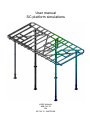
1
Calculation tools for
Series capacitor platforms
MIKA HYVÄRINEN
Master of Science Thesis
Stockholm, Sweden 2009
Calculation tools for
Series capacitor platforms
Mika Hyvärinen
Master of Science Thesis MMK 2009:96 MKN 020
KTH Industrial Engineering and Management
Machine Design
SE-100 44 STOCKHOLM
Examensarbete MMK 2009:96 MKN 020
Beräkningsverktyg för plattformar till
seriekompenseringsanläggningar
Mika Hyvärinen
Godkänt
Examinator
Handledare
2009-12-07
Ulf Sellgren
Ulf Sellgren
Uppdragsgivare
Kontaktperson
ABB FACTS
Henrik Säfström
Sammanfattning
ABB är världsledande inom kraft- och automationsteknik och deras lösningar förbättrar
prestanda och minimerar miljöpåverkan för energiföretag och industrier. ABB FACTS designar
utrustning och anläggningar för serie- samt faskompensering.
Detta examensarbete har utförts på ABB FACTS på avdelningen Mechanical Design (DM) i
Västerås. Syftet med projektet var att ta fram beräknings- och simuleringsverktyg för plattformar
som används av ABB FACTS i deras seriekompenseringsanläggningar. Examensarbetet har även
fungerat som en utvärdering av FEM programmet SolidWorks Simulation.
Examensarbetet inleddes med en förstudie där de normer och standarder som ABB FACTS
måste ha i åtanke vid konstruerande undersöktes. Eftersom större delen av dessa
seriekompenseringsanläggningar skickas till USA har den amerikanska standarden ASCE7-05
använts vid beräkningar av vind-, snö- och islaster. En referensram utvecklades där inhämtad
kunskap från förstudien och tidigare projekt på ABB presenteras. Därefter påbörjades
lastberäkningarna, modellerandet och simuleringarna av plattformarna samt utrustningen
ståendes på dessa plattformar. Verktygen som användes under projektet var Excel, SolidWorks
samt SolidWorks Simulation.
Resultatet av examensarbetet blev ett beräkningsprogram framtaget i Excel samt fyra modeller
för simuleringar i SolidWorks Simulation. Två av simuleringsmodellerna är uppbyggda så att de
kan användas på de bärbara datorer som de flesta av de anställda på ABB FACTS använder. Den
andra uppsättningen av modeller är tänkt att användas på ABB FACTS’s beräkningsdator.
Skillnaden mellan dessa modeller är att i de förenklade modellerna har utrustningen ståendes på
plattformarna ersatts med punktlaster. Modellerna har verifierats mot ABB Corporate Research.
Även en manual och en rapportmall har tagits fram. Manualen förklarar hur användaren på
enklast möjliga sätt kombinerar Excel beräkningarna med modellerna i SolidWorks Simulation.
Rapportmallen är utformad så att användaren snabbt och enkelt kan föra in resultaten från
beräkningarna samt simuleringarna för att sedan kunna skicka de till kund.
i
ii
Master of Science Thesis MMK 2009:96
MKN 020
Calculation tools for
Series capacitor platforms
Mika Hyvärinen
Approved
Examiner
Supervisor
2009-12-07
Ulf Sellgren
Ulf Sellgren
Commissioner
Contact person
ABB FACTS
Henrik Säfström
Abstract
ABB is one of the world’s leading engineering companies in power and automation technologies
and their solutions improve performance while lowering environmental impacts for energy
companies and industries. ABB FACTS designs equipment and plants for series and phase
compensation.
This thesis has been performed at ABB FACTS on the Mechanical Design (DM) department in
Västerås, Sweden. The purpose of the thesis was to develop and design calculations and
simulation tools for ABB FACTS’s standard series capacitor platforms. The thesis has also
served as an evaluation of the FEM program SolidWorks Simulation.
The thesis began with a pre study where the standards and requirements that ABB FACTS has to
consider during design were investigated. Since most of these series compensation plants are
sent to the United States, the American standard ASCE7-05 was used in the calculations of wind,
snow and ice loads. A reference frame was developed where knowledge obtained from the pre
study and previous projects in the ABB is presented. After that, the load calculations, modeling
and simulations of the platforms and equipment standing on these platforms began. The tools
used in this project were Excel, SolidWorks and SolidWorks Simulation.
The thesis resulted in a calculation program developed in Excel and four models for simulations
in SolidWorks Simulation. Two simulation models were modeled so that they can be used on the
laptops that most of the employees at ABB FACTS are using. The second set of simulation
models are designed to run on ABB FACTS’s calculation computer. These models contains in
addition to the platform also the equipment mounted on it. The models have been verified
against ABB Corporate Research. A manual and a report template have also been developed.
The manual explains how the user in the simplest way combines the Excel calculations with the
models in SolidWorks Simulation. The report template is designed so that the results from the
calculations and simulations easily can be entered and sent to the customer.
iii
iv
FOREWORD
This thesis work was performed at ABB FACTS in Västerås, Sweden, during the period June
2009 to November 2009.
I would like to thank Jerker Norberg, manager of Mechanical Design for great support and
interesting discussions during the work.
I would also like to thank my co-workers Patrick Alila and Erik Engsten for the excellent
guidance and good ideas through out this thesis.
Finally I would like to thank my supervisors, Ulf Sellgren at KTH and Henrik Säfström at ABB
FACTS.
Mika Hyvärinen
Västerås, November 2009
v
vi
NOMECLATURE
Descriptions for wind calculations
Symbol
Description
A
Af
Effective wind area [ m 2 ]
Area of open buildings and structures [ m2 ]
Ag
Gross area [ m 2 ]
Agi
Sum of the gross surface areas of the building or structure [ m 2 ]
Ao
Total area of openings in a wall that receives positive
Aoi
external pressure [ m 2 ]
Sum of the areas of openings in the building envelope [ m2 ]
As
a
B
b
Gross area of the solid freestanding wall [ m 2 ]
Width of pressure coefficient zone [ m ]
Horizontal dimension of building measured normal to wind direction [ m ]
Mean hourly wind speed factor
∧
b
c
Cf
Gust speed factor
Turbulence intensity factor
Force coefficient
F
Grigid
Design wind force for structures [ N ]
Gust effect factor for rigid buildings and structures
G flexible
Gust effect factor for flexible buildings and structures
gQ
Peak factor for background response
gR
gv
H
h
I
Iz
Peak factor for resonant response
Peak factor for wind response
Height of hill or escarpment [ m ]
Mean roof height of a building or height of structure [ m ]
Importance factor
Intensity of turbulence
K1 , K 2 , K 3
Multipliers to obtain K zt
Kd
Kh
Kz
K zt
L
Lz
Wind directionality
Velocity pressure exposure coefficient
Velocity pressure exposure coefficient
Topographic factor
Horizontal dimension of a building parallel to the wind direction [ m ]
Integral length scale of turbulence [ m ]
Lr
l
N1
Horizontal dimension of return corner for a solid freestanding wall [ m ]
Integral length scale factor [ m ]
Reduced frequency [ Hz ]
vii
n1
Building natural frequency [ Hz ]
p
Q
q
qz
R
Ri
s
V
W
z
z
zg
Design pressure to be used in determination of wind loads [ N / m 2 ]
Background response factor
Velocity pressure [ N / m 2 ]
Velocity pressure evaluated at height z above ground [ N / m 2 ]
Resonant response factor
Reduction factor
Vertical dimension of the solid freestanding wall [ m ]
Basic wind speed [ m / s ]
Width of building [ m ]
Height above ground level [ m ]
Equivalent height of structure [ m ]
Nominal height of the atmospheric boundary layer used
zmin
Exposure constant
Gust-speed power law exponent
α
∧
α
α
β
∈
∈
Reciprocal of α
Mean hourly wind-speed power law exponent
Damping ratio, percent critical for buildings or other structures
Ratio of solid area to gross area for solid freestanding wall
Integral length scale power law exponent
Descriptions for snow calculations
Symbol
Ce
Cs
Ct
hb
hc
Description
hd
ho
I
lu
L
pd
Exposure factor
Slope factor
Thermal factor
Height of balanced snow load [ m ]
Clear height from top of balanced snow load to closest
point on adjacent upper roof [ m ]
Height of snow drifts [ m ]
Height of obstruction above the surface of the roof [ m ]
Importance factor
Length of the roof upwind of the drift [ m ]
Roof length parallel to the ridge line [ m ]
Maximum intensity of drift surcharge load [ N / m 2 ]
pf
Snow load on flat roofs [ N / m 2 ]
pg
Ground snow load [ N / m 2 ]
ps
S
Sloped roof snow load [ N / m 2 ]
Roof slope run for a rise of one
viii
θ
W
Roof slope on the leeward side ( ° )
Horizontal distance from eave to ridge [ m ]
ρs
Snow density [ N / m3 ]
Descriptions for ice calculations
Symbol
Description
As
Surface area of one side of a flat plate or the projected
Ai
D
Dc
fz
Ii
Iw
K zt
t
td
area of complex shapes [ m 2 ]
Cross-sectional area of ice [ m 2 ]
Diameter of a circular structure or member [ m ]
Diameter of the cylinder circumscribing an object [ m ]
Factor to account for the increase in ice thickness with height
Importance factor
Importance factor
Topographic factor
Nominal ice thickness due to freezing rain at a height [ m ]
Design ice thickness [ m ]
Vi
Volume of ice [ m3 ]
pi
z
Uniform distributed ice loads [ N / m 2 ]
Height above ground [ m ]
ρi
Ice density [ N / m3 ]
Abbreviations
ABB
ASEA Brown Boveri
ASCE
American Society of Civil Engineers
CAD
Computer Aided Design
FACTS
Flexible AC Transmission System
FEM
Finite Element Method
MOV
Metal Oxide Varistors
RIV
Radio Interference Voltage
SC
Series Capacitor
ix
x
TABLE OF CONTENTS
1 INTRODUCTION
1
1.1 BACKGROUND
1.2 PURPOSE
1.3 DELIMITATIONS
1.4 METHOD
1.5 BENEFIT FOR ABB FACTS
1
1
1
1
2
2 FRAME OF REFERENCE
3
2.1 SERIES COMPENSATION
2.2 SERIES CAPACITOR
2.2.1 CAPACITOR BANK
2.2.2 METAL OXIDE VARISTORS
2.2.3 TRIGGER EQUIPMENT
2.2.4 DAMPING CIRCUIT
2.2.5 SPARK GAPS
2.2.6 FIBER OPTIC LINK
2.2.7 BY-PASS BREAKER
2.2.8 PLATFORM
2.3 LOADS
2.3.1 WIND LOADS
2.3.2 SNOW AND ICE LOADS
2.3.3 DEAD LOADS
2.3.4 EARTHQUAKES
2.4 NORMS AND STANDARDS
2.4.1 WIND LOADS
2.4.2 SNOW LOADS
2.4.3 ICE LOADS
3
4
5
6
6
6
7
7
7
7
9
9
9
10
10
10
10
10
10
3 METHOD
11
3.1 LOAD COMBINATIONS
3.2 LOAD AND TERRAIN CATEGORIES
3.3 WIND LOADS
3.4 SNOW LOADS
3.4.1 FLAT ROOFS
3.4.2 SLOPED ROOFS
3.4.3 RAIN ON SNOW
3.5 ICE LOADS
3.5 DEAD LOADS
3.6 PRE-STRESS LOADS
3.7 MODELING
3.7.1 PLATFORM
3.7.2 SUPPORTING INSULATORS
3.7.3 CAPACITOR BANK
3.7.4 DAMPING CIRCUIT
3.7.5 METAL OXIDE VARISTORS
11
11
12
17
17
18
19
20
21
21
22
22
22
23
24
24
xi
3.8 SIMULATION
3.8.1 BEAM OR SHELL ELEMENTS
3.8.2 CONNECTIONS AND FIXTURES
3.8.3 LOADS
3.4.4 MESH
25
25
25
26
28
4 RESULTS
29
4.1 THE CALCULATION TOOL
4.2 THE SIMULATION TOOL
4.1 THE USER MANUAL
4.1 THE REPORT TEMPLATE
29
30
30
30
5 VERIFICATION
31
6 DISCUSSION AND CONCLUSIONS
34
7 RECOMMENDATIONS AND FUTURE WORK
36
8 REFERENCES
37
APPENDIX A: Wind map
38
APPENDIX B: Snow map
40
APPENDIX C: Ice map
42
APPENDIX D: Cross sections
44
APPENDIX E: XML code
45
APPENDIX F: Report template
46
APPENDIX G: USER MANUAL
47
xii
1 INTRODUCTION
In this chapter the background, the purpose, delimitations and the method used in this project
are presented.
1.1 Background
ABB FACTS (Flexible AC Transmission System) [1] is a part of ABB Power Systems [2] which
designs equipment and plants for series compensation. These series compensation plants, also
know as series capacitors (SC’s) [3], are electrical installations for increasing power transmission
capacity. Series capacitors eliminate the steady-state voltage drop along the power lines as well
as the voltage fluctuations associated with start-ups of large electrical loads.
In this thesis, calculation and CAD models of the standard platforms that ABB FACTS uses in
their series compensation plants are modeled and simulated based on the American standard
ASCE7-05 [4].
1.2 Purpose
The purpose of this thesis is to design and develop calculations and simulation tools for ABB
FACTS’s standard series capacitor platforms in SolidWorks [5] and SolidWorks Simulation [6].
Different load standards and requirements will be presented and interpreted. The models will be
built after the two types of standard platforms used in ABB FACTS. These models will be
designed in such a way that changes in dimensions and load cases easily can be made.
A manual and a report template will also be presented. The manual will explain the structure of
the models and the procedure of making changes in them. The manual will explain how the
inputs are obtained and which parameters are to be fed into the models, but also describe how the
results from the simulations in a simple way can be transferred in to a report. The manual will be
written in Swedish and in English.
1.3 Delimitations
Calculation and CAD tools will only be developed for the two types of standard platforms that
ABB FACTS uses in their series capacitors. This thesis work confines to the American standard
of ASCE7-05 in all load calculations since most of these series platforms are delivered to the
United States. Only static loads will be considered, seismic and dynamic calculations are omitted
entirely. No frequency analysis will be made in this project as this has previously been done at
ABB for these platforms.
1.4 Method
A pre study will be performed to investigate the standards and requirements that ABB FACTS
has to consider when a series compensation plant is designed. The American standard of
ASCE7-05 will be used in calculations of wind, snow and ice loads. These load calculations will
be made in Excel [7] spreadsheets so that the loads acting on the standard platforms easily can be
obtained.
1
CAD models of these standard platforms will be created in SolidWorks so that any changes in
platform types, dimensions or load cases easily can be made. The task is also to examine whether
these CAD models are to be built by beam or shell elements.
The evaluation of these standard platforms will be performed by using SolidWorks Simulation
(former known as Cosmos Works [8]). The results from the FEM simulations will be compared
with results from ABB Corporate Research [9] in a sharp scenario.
The manual that describes the approach of these calculations and simulations will be written so
that the user easily can follow the reasoning step by step.
Finally, a report template will be developed together with the employees at ABB FACTS so that
it easily can be modified from one project to another. It will be designed so that the results from
the calculations and simulations in a simple way can be entered and sent to the customer.
1.5 Benefit for ABB FACTS
This thesis will result in following benefits for ABB FACTS:
•
Avoiding outsourcing all calculations and simulations at ABB Corporate Research, this
will streamline the projects.
•
More reliable results, this will reduce the risk of over dimensioning.
•
Better and more reliable reporting data to the customers.
•
Evaluation of the FEM program SolidWorks Simulation. It is desirable to find out if this
program is sufficiently strong and developed for the tasks that ABB FACTS encounters
during their projects.
2
2 FRAME OF REFERENCE
This chapter presents the theoretical reference frame and provides support and understanding
for the remainder of the report.
2.1 Series compensation
The reason for series compensation is essentially to increase transmission capacity into the
power lines by reducing the reactance in it. The maximum capacity that can be transmitted from
node 1 to node 2 at high voltage electricity can be approximated from equation 1 and 2 below.
⎛ U ⋅U
⎞ U ⋅U
P1− 2 = max ⎜ 1 2 sin(δ ) ⎟ = 1 2
X
⎝ X
⎠
(1)
U = f ( P, Q )
(2)
U1 and U 2 represents the voltages at either end of the nodes, whereas δ denotes the angular
difference of the two voltages. X is the reactance of the transmission circuit, while P and Q
denote the received active and reactive power.
Equation 1 suggests that the greater the reactance of a power line is the less power can be
transferred through it. By installing series capacitors on the power line, the total reactance of the
circuit can be reduced and maximum transmitted power can be provided. In Figure 1 below the
difference between a power grid with and without a series capacitor is shown [10][13].
Figure 1. Power grid with and without a series capacitor [ABB Power Technologies AB, 2005].
3
2.2 Series capacitor
Long distances are often the main reason for the usage of series capacitors. Series capacitors
work like boosters as they eliminates the steady-state voltage drop along the power lines as well
as voltage fluctuations associated with high load start-ups.
A standard one phase ABB series capacitor is constructed as shown in Figure 2, 3 and 4. It has a
capacitor bank (a), several metal oxide varistors (b), a trigger equipment (c), a damping circuit
(d), two spark gaps (e), a fiber optic link (f), a control platform (g), a by-pass breaker (h) and
several Rodurflex’s (i). Every component is either standing on or connected to an insulated steel
platform. It is this platform including the insulators supporting the platform that this thesis
focuses on. Detailed information about the equipment standing on the platform is not presented
in this public report due to confidentiality.
b
a
h
f
i
Figure 2. Layout of a one phase series capacitor.
d
e
g
Figure 3. Layout of a one phase series capacitor.
4
Figure 4. Layout of a one phase series capacitor.
2.2.1 Capacitor bank
The capacitor bank shown in Figure 5 consist of capacitor units connected in parallel in
sufficient number to handle the highest continuous current required of the load downstream of
the bank. These parallel arrangements, or groups as they are called, are connected in series to
provide the required ohmic value of compensation needed to provide the required voltage rise
under the given operating conditions.
Figure 5. Capacitor bank.
5
2.2.2 Metal oxide varistors
The metal oxide varistors (MOV) shown in Figure 6 protects the capacitors against over-voltage.
During ordinary conditions, all the power flows through the capacitor bank and when a fault
arises the varistors limits the voltage across the capacitors.
Figure 6. Metal oxide varistors.
2.2.3 Trigger equipment
The trigger equipment is used to force trig the spark gaps and enable the by-pass of the series
capacitors in situations where the varistors capacity is not sufficient to absorb the excess current
during a fault sequence.
2.2.4 Damping circuit
The damping circuit consists of two components, the reactor and the damping resistor. The
purpose of the damping circuit shown in Figure 7 below is to limit and damp the discharge
current caused by spark gap or closing of the switch.
Figure 7. Damping circuit.
6
2.2.5 Spark gaps
Spark gaps are normally used for immediate by-pass of the metal oxide varistors and the
capacitors at internal or severe external faults or at demanding short circuit levels and duty
cycles.
2.2.6 Fiber optic link
For communication between platform and ground, fiber optic transmission links are utilized.
2.2.7 By-pass breaker
The bypass breaker is an Auto-Puffer circuit breaker. With a closing time of half of what the
other bypass switches have, makes it the fastest bypass switch available on the market for series
compensation applications. This enables a great saving on metal oxide varistors in the protective
scheme.
2.2.8 Platform
There are two types of standard platforms, one with two transverse main beams and one with
three, this is shown in Figure 8 below. The beam arrangement for a platform is adjusted
regarding the spatial spreading of the equipment placed on it. The dimensions of the beams are
usually limited to two or three different types.
Figure 8. The two and the three beam platform.
The platform module includes supporting insulators, the platform (steel structure) and supporting
structure for all equipment placed on the platform. Handrails, corona protection, ladder and other
details related to the platform are also included. Listed below is a brief description on some of
the sub modules.
• Platform, steel structure.
ABB uses a hot dip galvanized steel structure in the design of the platforms. The platforms
are designed with respect to easy handling and are completely prefabricated in the workshop
to be bolted together at the construction site. For the personal safety the platforms are
provided with a steel grating. The stressed beams have a material strength of 355 MPa, the
non stressed beams have normally a lower material strength.
7
• Supporting insulators
The insulators are made of homogeneous porcelain and can handle a torque of 8 kNm due to
the mechanical joints located between the insulators and the platforms (steel structure and
isolator platform), see Figure 9. The solution and design is depending on environment,
voltage level and mechanical loads from the platform.
Insulator
Mechanical joints
Insulator platform
Figure 9. A supporting insulator, broken view.
• Rodurflex
The Rodurflex is not an ABB specific component, it is manufactured by LAPP Insulators
[11]. The Rodurflex consists of a fiberglass core which is covered with 3 mm thick high
temperature vulcanized silicone rubber that improves the systems mechanical characteristics
but also protects the core during handling and installation. Since the insulators are made of
porcelain, the Rodurflex’s are important because they absorb the tensions which the
insulators are exposed to. A Rodurflex in a standard design can handle tensions of 210 kN
[12].
• Corona protection.
This sub module protects the platform and the equipment standing on it against radio
interference voltage (RIV) and corona. There are two different aluminum profiles depending
on voltage level. Fastening system is standardized to one standard solution.
The corona protection also works as a handrail. The aluminum profile for the handrail is
specially developed for ABB and after many years of experience it has shown that this is the
best solution. The advantage with using the profile is the protective solution for corona
protection and the easy erection. It has also the mechanical strength to prevent personal from
falling of the platform.
• Ladder
The ladder gives a safe access to the platform. It is easy to handle and the turntable design
minimize required space. The ladder can be equipped with interlocking to prevent human
errors. There are two standard ladder solutions and one ladder design. The length of the
ladder is adjusted depending on voltage level (length of the insulators).
8
• Equipment support
There are two different standard solutions to support the varistors. Choice of support is
depending on mechanical loads. For the reactor there is only one type of leg with variations
on the height.
2.3 Loads
A dynamic load is a load that gives rise to the supplement forces and deformations as a result of
accelerations in the structure and load. A load is considered static if it does not cause
significance acceleration for the structure.
Many loads should be considered as dynamic, such as rotating loads, the load of people and
machinery shocks. In many cases the structures dynamic conditions are not treated
computationally and therefore these calculations can be performed in the same way as for static
loads.
At pulsating or alternating loads there are risks of resonance if the frequency of the load is close
to the structures eigenfrequency. The dynamic effects can usually be neglected if the load
frequency is one third of the structures eigenfrequency. If the load frequency is much higher than
the eigenfrequency of the structure, the impact of load variations can be neglected due to the
structure which acts as a vibration damper [14].
Given in this thesis is that the platforms should be considered as rigid with an eigenfrequency of
2 Hz. These calculations have been done in previous projects and will not be included in this
report [15].
2.3.1 Wind loads
The wind load is inherently a dynamic load which means that its acceleration is affecting the
structure. For structures with high stiffness and damping, that does not need to consider the
structural vibration characteristics for the determination of wind load, the wind load can be
treated as a static load. The wind load can sometimes be a fatigue loading. This applies mainly
when the wind load causes a large number of oscillations of the structure.
The velocity of the wind affecting the structure depends on the geographic location of the
structure, surrounding terrain and the height of the structure. The effect of location is described
by the reference wind speed and is mostly obtained from wind maps [14] [4].
2.3.2 Snow and ice loads
Snow loads are in the most cases assumed to be variable and bounded loads and determined as
the weight per horizontal area. When determining the snow loads, the form of the structure has to
be taken into account due to wind effects and risks of sliding. The characteristic snow pressure is
often retrieved from snow maps.
Ice loads are mostly generated by changes in the temperature and freezing rain. Freezing rain
occurs when warm moist air is forced over a layer of subfreezing air at the earth’s surface. The
precipitation usually begins as snow that melts as it falls through the layer of warm air aloft. The
drops then cool as they fall through the cold surface air layer and freeze on contact with the
structure [16] [4].
9
2.3.3 Dead loads
A dead load is a static load and consists of the weight of all materials incorporated with the
structure, including the weight of all components standing on or in the structure [4].
2.3.4 Earthquakes
Depending on country and region, there is sometimes a risk of earthquakes. Earthquakes consist
of dynamic forces that occur irregularly over time and to calculate these forces seismic studies
are required. An alternative is to use sophisticated FEM programs, but ABB FACTS has not
direct access to these programs and therefore are these kind of calculations omitted entirely in
this thesis.
2.4 Norms and standards
ABB FACTS is currently using several different standards. It is essentially the costumer’s
geographical market that determines the use of norms and standards in a project. Since most of
these platforms are delivered to the United States, the American standard ASCE7-05 is used
throughout this thesis.
ASCE or American Society of Civil Engineers is an ANSI accredited standards development
organization that produces consensus standards under direction of the Codes and Standards
Activities Committee.
The ASCE standard 7-05 provides minimum load requirements for the design of buildings and
other structures that are subject to building code requirements. Wind, snow, ice, dead and live
loads as well as appropriate load combinations are interpreted and determined in this standard
[4].
2.4.1 Wind loads
ASCE7-05 provides three different approaches to determine the wind load from which the
designer can choose. An expanded simplified method in which the designer can select the wind
pressures directly without any calculation if the building meets all the requirements, one wind
tunnel procedure and one analytical method. In this project the analytical method is used
consistently.
2.4.2 Snow loads
The method of calculating the snow loads as ASCE7-05 offers is designed by static analysis of
extreme values of snow amounts over a period of 50 years in the United States.
2.4.3 Ice loads
This chapter deals with various ice scenarios, such as freezing rain, in-cloud icing, wind on ice
and hoarfrost.
2.4.4 Dead loads
The calculation of dead loads is very straight on in this standard and only a few pages are
speared to these calculations.
10
3 METHOD
This chapter describes the approach of load calculations, CAD modeling and FEM simulations.
3.1 Load combinations
Structures, components, and foundations shall, according to ASCE7-05, be designed so that their
design strength equals or exceeds the effects of the factored loads in equation 3.
1.2 ⋅ D + 1.6(Sor R) + 0.8 ⋅ W
(3)
The coefficient D stands for the dead loads, S for snow loads, R for rain loads and W for the
static wind loads.
ABB Corporate Research uses two design load combinations when designing series capacitor
platforms. Equation 4 is for the transverse Y-direction and equation 5 for the longitudinal Xdirection of the platform.
W−Y+T+D
(4)
W−X+T+D
(5)
T in equation 4 and 5 represents the terminal forces, Y stands for forces in the transverse
direction of the platform and X is forces in the longitudinal direction.
3.2 Load and terrain categories
When calculating on wind, snow and ice loads the ambient roughness has to be considered.
Below follows a categorization of terrain roughness from ASCE7-05.
Exposure B shall apply where the ground surface roughness condition, as defined by Surface
Roughness B, prevails in the upwind direction for a distance of at least 792 m or 20 times the
height of the building, whichever is greater.
Surface Roughness B: Urban and suburban areas, wooded areas, or other terrain with numerous
closely spaced obstructions having the size of single-family dwellings or larger.
Exposure C shall apply for all cases where Exposures B or D does not apply.
Surface Roughness C: Open terrain with scattered obstructions having heights generally less than
9 m. This category includes flat open country, grasslands and all water surfaces in hurricane
prone regions.
Exposure D shall apply where the ground surface roughness, as defined by Surface Roughness
D, prevails in the upwind direction for a distance greater than 1524 m.
Surface Roughness D: Flat, unobstructed areas and water surfaces outside hurricane prone
regions. This category includes smooth mud flats, salt flats and unbroken ice.
11
3.3 Wind loads
The design wind loads are determined according to equation 6 below.
F = qz ⋅ G ⋅ C f ⋅ A f
(6)
The velocity pressure qz is calculated from equation 7. The numerical coefficient 0.613 is only
used when no other climate data is available for the region.
qz = 0.613 ⋅ K z ⋅ K zt ⋅ K d ⋅V 2 ⋅ I
(7)
The velocity pressure exposure coefficient K z can be obtained from a Table 1, but the most
accurate value on K z is given by equation 8.
⎛ 15 ⎞
K z = 2.01⎜ ⎟
⎜ zg ⎟
⎝ ⎠
2
α
(8)
The terrain exposure constants α and z g in equation 8 are obtained from Table 2 on the next
page.
Table 1. The velocity pressure as a function of height and roughness category [ASCE, 2006].
12
Table 2. Terrain exposure constants [ASCE, 2006].
The topography factor K zt is calculated according to equation 9, but the most critical approach is
when K zt reaches the value 1. For that reason K zt will be set to 1 through all calculations and
simulations in this thesis work.
K zt = (1 + K1 + K 2 + K 3 )
2
(9)
The wind directional factor K d is obtained from Table 3 below.
Table 3. The wind directional factor as a function of structure type [ASCE, 2006].
The speed of wind V varies greatly depending on the country and region. Therefore, this
constant is determined from a wind map. In Appendix A, a wind map of the United States is
presented.
The importance factor I used in equation 7 diversifies from 0.77 to 1.15 depending on if the
region in which the plant or building is standing has a higher risk of hurricanes. This is shown in
13
Table 4 below. Only category IV (four), which includes communication towers, fuel storage
tanks, cooling towers and electrical substation structures, is treated in this thesis.
Table 4. The importance factor of the wind loads [ASCE, 2006].
Depending on whether the structure is considered as rigid (natural frequency, f ≥ 1 Hz ) or
flexible (natural frequency, f < 1 Hz ) the gust effect factor G is determined in different ways.
For a flexible structure the gust effect factor is calculated according to equation 10 and for a rigid
structure according to equation 11.
⎛ 1 + 1.7 ⋅ I g 2 ⋅ Q 2 + g 2 ⋅ R 2
Q
R
z
G flexible = 0.925 ⎜
⎜
1 + 1.7 ⋅ gv ⋅ I z
⎝
⎞
⎟
⎟
⎠
⎛ 1 + 1.7 ⋅ gQ ⋅ I z ⋅ Q ⎞
Grigid = 0.925 ⎜
⎜ 1 + 1.7 ⋅ g ⋅ I ⎟⎟
v
z
⎝
⎠
I z which is the intensity of turbulence at height z is calculated by equation 12.
(10)
(11)
1
⎛ 10 ⎞ 6
Iz = c ⎜ ⎟
⎝ z ⎠
(12)
The terrain exposure constant c is obtained from Table 2, the equivalent height of the structure
z is defined as 0.6 times the height of the structure, but not less than zmin shown in Table 2.
The background response Q used in both equation 10 and 11 is given by equation 13 below.
Q=
1
⎛ B+h⎞
1 + 0.63 ⎜
⎜ L ⎟⎟
⎝ z ⎠
(13)
0.63
The integral length scale of turbulence at the equivalent height Lz is calculated according to
equation 14 below. The terrain constants l and ∈ used in equation 14 are listed in Table 2.
∈
⎛ z ⎞
Lz = l ⎜ ⎟
⎝ 10 ⎠
(14)
14
gQ and gv which represents the peak factors of background and wind response shall according to
ASCE7-05 always be taken as 3.4. g R , the peak factor for resonant response is given by
equation 15, where n1 stands for the structures natural frequency.
0.577
(15)
g R = 2 ln(3600 ⋅ n1 ) +
2 ln(3600 ⋅ n1 )
R , the resonant response factor used in equation 10 for calculating the flexible guest factor is
obtained from equation 16 below
1
R=
R ⋅ R ⋅ R (0.53 + 0.47 ⋅ RL )
(16)
β n h B
where
7.47 ⋅ N1
Rn =
(17)
5
3
(1 + 10.3 ⋅ N1 )
N1 =
n1 ⋅ Lz
(18)
Vz
α
⎛ z ⎞
Vz = b ⎜ ⎟ V
⎝ 10 ⎠
1
(1 − e −2η ) for η > 0
η 2η 2
Rl =1for η = 0
Rl =
1
(19)
−
(20)
(21)
The subscript l in equation 20 and 21 shall be taken as h , B and L .
4.6 ⋅ n1 ⋅ h
Rl = Rh by setting η =
Vz
(22)
Rl = RB by setting η =
4.6 ⋅ n1 ⋅ E ⋅ B
Vz
(23)
Rl = RL by setting η =
15.4 ⋅ n1 ⋅ L
Vz
(24)
The force coefficient C f used in the main equation for determining the design wind loads varies
slightly depending on the member geometry and is most easily retrieved from Table 5 below.
Table 5. The force coefficient for round and flat members [ASCE, 2006].
15
∈ in Table 5 represents the ration of solid area to gross area. This constant should not be mixed
up with the terrain constant ∈ in Table 2.
Af used in equation 6 is the projected area normal to the wind.
16
3.4 Snow loads
Depending on the roof type, the snow loads are calculated in different ways. Below follows the
calculations used depending on difference in roof type.
3.4.1 Flat roofs
For a flat roof the snow loads are determined by equation 25. A roof classifies as flat if its slope
is less than 5 degrees.
p f = 0.7 ⋅ Ce ⋅ Ct ⋅ I ⋅ pg
(25)
The exposure factor Ce and the thermal factor Ct are obtained from Table 6 and Table 7 below.
Table 6. The exposure factor [ASCE, 2006].
Table 7. The thermal factor [ASCE, 2006].
I , the importance factor is found in Table 8. As mentioned in chapter 3.3 Wind loads this thesis
will only treat buildings classified as category IV (four), which includes electrical substations
and plants, so this factor is set to 1.2 through all snow load calculations.
Table 8. The importance factor depending on building category [ASCE, 2006].
The ground snow loads
pg used in equation 25 is obtained from a snow map. Appendix B
shows a snow map for the United States. Snow loads are set to zero in Hawaii, and for colder
locations in Alaska Table 9 is used.
17
Table 9. Ground snow loads for locations in Alaska [ASCE, 2006].
3.4.2 Sloped roofs
Snow loads acting on sloped roof is assumed to act on a horizontal projection of that surface.
The sloped roof loads are obtained by multiplying the flat roof snow loads by the slope roof
factor Cs , shown in equation 26 below.
ps = C s ⋅ p f
(26)
For warm roofs ( Ct ≤ 1 as determined from Table 7) the slope factor is determined by using
Figure 10a.
Cold roofs are those with a thermal factor larger than 1.0. For a cold roof with a Ct value of 1.1
the slope factor is determined by Figure 10b and for those with a Ct value of 1.2 the Figure 10c
is used.
Figure 10. The slope factor for warm and cold roofs [ASCE, 2006].
18
3.4.3 Rain on snow
For locations where the ground snow loads are 0.96 kN / m 2 or less, but not zero, and for roofs
with slopes less than the width of the building divided by the factor 15.2, a 0.24 kN / m 2 rain on
snow surcharge shall be applied.
19
3.5 Ice loads
The uniform distributed ice loads pi due to freezing rain are calculated from equation 27
pi =ρi ⋅ Ai ⋅ g
(27)
were ρi represents the density of the ice and shall not be set less than 900 kg / m3 . The cross
sectional area of the ice Ai is obtained from equation 28.
Ai = π ⋅ td ( Dc + td )
(28)
The design ice thickness td used in the equation for the cross sectional area is calculated from
equation 29.
td = 2.0 ⋅ I i ⋅ f z ( K zt )0.35
(29)
The importance factor I i is set to 1.25 for electrical substations and plants. For other structures,
see Table 10.
Table 10. The importance factor for ice thickness depending on building category [ASCE, 2006].
f z is a height factor and is used to increase the radial ice thickness above the ground and is
determined from equation 30.
⎛ z ⎞
fz = ⎜ ⎟
⎝ 10 ⎠
0.10
for 0 m < z ≤ 275 m
(30)
For altitudes above 275 m the height factor is set to 1.4.
The topographic factor K zt is the same as in the wind calculations, and as mentioned in chapter
3.3 Wind loads, the most critical approach is when K zt reaches the value 1. Therefore is this
constant set to 1 through all calculations and simulations in this report.
Dc in equation 28 is the characteristic diameter of the cylinder circumscribing the profile which
the structure is constructed by. Appendix D shows the characteristic diameter for a variety of
cross sections.
20
3.5 Dead loads
After careful consideration together with higher courts at ABB FACTS, the dead load will in
addition to the platform with supporting insulators only consist of the capacitor bank, the
damping circuit and the metal oxide varistors. These components weigh, compared to the other
equipment on the platform, considerably more. It is also these components that have the largest
effective load surface. Depending on the platform type and size, the total dead load varies from
40000 to 60000 kg.
When calculating on the weight of the platform, 105 kg / m 2 can be used as a reference figure.
This gives, in a standard version, a two beam platform a total weight of approximately 9000 kg
and a three beam platform a total weight of about 12000 kg.
The weight of a supporting insulator depends on the length of it, which in turn depends on the
plants voltage level. Somewhere between 700 and 1000 kg can be expected that an insulator in
its standard version weighs.
The capacitor bank has a weigh of about 9000 kg per stack. The number of stacks varies
depending on the plant size and location, but in a typical case the capacitor bank have two stacks
and weighs 25000 kg on a two beam platform. On a three beam platform the capacitor bank have
four stacks, this result in a weight of 50000 kg.
The weight of a damping circuit varies slightly depending on the plant size, but on average, this
module weighs about 2000 kg.
The metal oxide varistors have a weight of approximately 4500 kg, plus minus a couple of
hundred kilos depending on the number of varistors units and terminals.
3.6 Pre-stress loads
Pre-stressing forces in the diagonally mounted Rodurflex’s, see Figure 11, are in this report
named as pre-stress loads. These loads are for the most of ABB’s plants set to 20 kN.
Figure 11. The Rodurflex with black arrows representing the pre-stress loads.
21
3.7 Modeling
No deeper breakdown of the model creating will be presented in this chapter, the reader is
assumed to possess basic knowledge in this area. Dimensions and other sensitive information
will not be presented in this general report due to confidentiality. The models are modeled so that
the dimensions and structure quickly and easily can be modified. All models are constructed of
3D sketches. In addition to regular models, simplifications are developed to facilitate and speed
up the simulations.
3.7.1 Platform
The base of the platform consists of either two or three HEA beams, depending on platform type.
Across these beams are four capacitor beams, four apparatus support beams and several grating
support beams placed, all beams of the type HEA. The cross beams, marked blue in Figure 12,
stiffens the platform. These cross beams together with the outer frame are modeled from an Lprofile. The command “Structural Remember” is used for all beams in the platform, this feature
keeps the model size down.
Figure 12. CAD model of a three beam platform with blue marked cross beams.
3.7.2 Supporting insulators
The supporting insulators are modeled in three subassemblies; the porcelain insulator, the
insulator platform and the upper end joint.
The porcelain insulator is modeled as a single solid piece. With the command “Revolve” in
SolidWorks a 3D profile is created from a 2D sketch. The material in this 3D profile is set to
homogenous porcelain.
The insulator platform consists of several parts, see Figure 13 on the next page. On top of the
bottom plate, which is the base of the model and created by an “Extrude”, stands a square tube
built by the command “Structural Member”. Four support plates are connecting the bottom plate
with the square tube. Above the square tube are two square plates located with a mechanical joint
between them. These three elements, along with the supporting plates, are modeled with the
command “Extrude”.
22
Figure 13. CAD model of the supporting insulator platform.
The upper end joint consists of a circular and a square plate, between these is the mechanical
joint located. The material in the insulator platform and the upper end joint is set to galvanized
steel.
3.7.3 Capacitor bank
The capacitate stack, shown in Figure 14 below, consists only of a capacitor unit, a capacitor
frame and an insulator. These components are then multiplied by using linear and circular
patterns, this in order to reduce the model size. The capacitor frame is modeled as a solid block
with “Extruded Cuts” in several directions. The capacitor unit is an extruded body with a circular
connection. A revolved 2D sketch forms the insulators.
Figure 14. CAD model of a capacitor stack.
23
3.7.4 Damping circuit
The damping resistor is mainly designed with the “Revolve” and the “Extrude” command. The
connections are modeled with the “Sweep” command.
The reactor and the insulators which the reactor is standing on are modeled using “Revolve”.
The mounts between the reactor and the insulators are made from two L-profiles by using
“Structural Member”. The other components in this assembly are made from by “Extrude”. Both
the reactor and the damping resistor are shown in Figure 15 below.
Figure 15. CAD model of the damping circuit.
3.7.5 Metal oxide varistors
The tripod to the metal oxide varistors is modeled from six UPE beams and four ABB specific
beams, using the “Structural Remember” feature. The varistors are designed with the “Revolve”
and “Linear Pattern” command. The result is shown in Figure 16.
Figure 16. CAD model of the metal oxide varistors.
24
3.8 Simulation
As mentioned in chapter 3.7 Modeling, there are in addition to regular models also
simplifications, this results in four simulation models; two for three beam platform and two for
two beam platform. One of the models in each platform type is designed to run on laptops and
does not containing the equipment standing on the platform. The equipment and the forces acting
on them are replaced by point forces. The second set of simulation models are designed to run on
ABB’s calculation computer. These models contains in addition to the platform also the
equipment mounted on it. The results between the regular and the simplified models do not
differ. The main reason for using the complete regular models is to give the costumer a more
accurate visual perceptive.
3.8.1 Beam or shell elements
The task to examine whether the models are to be built up of beam or shell elements was
developed at a time when ABB still was using Cosmos, today known as SolidWorks Simulation.
Cosmos gave the user the ability to choose a way of meshing the model at the beginning of each
study. In SolidWorks Simulation, this feature has been removed and replaced with an automatic
“Mixed Mesh”. By default, any surface bodies will be treated as shell elements, any structural
members will be treated as beam elements, and everything else will be treated as solid elements.
The platforms, excluding the outer frames, are in these simulations meshed as beams as this
speeds up the simulations. The outer frames are meshed as solid since wind loads are affecting
on these surfaces and SolidWorks Simulation does not support pressure on beam elements. The
support insulators are meshes as solid.
3.8.2 Connections and fixtures
When using both beam and solid elements in a simulation, bonded contact sets between these
elements are needed. Bonded entities behave as if they were welded or bolted.
Rigid connectors are placed between the insulator platform and the square tube standing on it.
These rigid connectors rigidly connect faces from one solid body to faces from another solid
body. In this case rigid connectors simulate the welds, which have been removed to allow the
simulations.
To simulate the foundation bolts, fixed support is used in the holes on the insulator platform, see
Figure 17.
Figure 17. Fixed support on the insulator platform.
25
The mechanical joints in the supporting insulators, illustrated in Figure 18, have a structure that
resembles a universal joint. These joints have in the simulation models been replaced by simple
square blocks. To make the models as close as to reality, these blocks are in the ends connected
with “Hinge” connections. The “Hinge” connections are locked so that they only allow
movement in two directions and entirely limit rotations along the insulators.
Figure 18. The mechanical joint in the supporting insulators.
3.8.3 Loads
The equivalent force magnitude acting on the platform generated by pressure is equal to the
pressure times the area, this is shown in Figure 19 for an insulator on the next page. The size of
the wind pressure depends on the height of the platform since the pressure increases with
increasing distance from the ground. It is important to apply the right pressure on the right area
and height.
In the same way as for wind loads, force equals pressure times area, the snow and ice loads are
applied on the platform and equipment. The advantage with calculating forces in this way is that
the user only needs to calculate the pressure acting on the surface. In the regular models,
SolidWorks determines the surface areas and hence the forces acting on the platform and
equipment. In the simplified models the user has to determine the effective load surface,
preferably from a dimensioned drawing and manually calculate the magnitude of the force.
In addition to the external forces there are weights of the equipment, dead loads, affecting on the
platform. These forces are in the simplified models set as point masses with the direction to the
ground. In the regular models, SolidWorks generates these loads if the right material properties
are given for all components.
26
Figure 19. An insulator with the right pressures at the right areas.
The diagonal mounted Rodurflex’s and the pre-stress loads located in them are simulated with
tension springs. These springs have an axial stiffness of 2.5 ⋅106 N/m and a tension preload force
of 20 kN. The springs are attached to the support plates down on the insulator platform and the
other end is attached at the upper end joint on the support insulator standing next, this is
illustrated in Figure 20 below.
Figure 20. Two supporting insulators with the tension spring between them.
27
3.4.4 Mesh
In these models, SolidWorks Simulation only generates a working mesh when all settings are set
to the highest and finest (this is a documented error that often occurs for large assemblies), this
gives that no convergence study can be done for the results generated by SolidWorks Simulation.
The elements in the models have a global size of 50 mm and a tolerance of 3 mm. The few
available mesh settings are shown in Figure 21.
Figure 21. Mesh settings in SolidWorks Simulation.
The mesh for a simplified three beam platform is shown in figure 22 below.
Figure 22. The mesh of a three beam platform.
28
4 RESULTS
This chapter presents and summarizes the results from this thesis.
4.1 The calculation tool
The calculations are made as previously mentioned in Excel with a work sheet for each load
calculation, see Figure 23. The user only needs to have the dimensions of the plant and the
geographic location in mind, the calculation tool generate the right wind, snow and ice pressure
as a function of height. The XML code for the Excel program is available at Appendix E.
Figure 23. The Excel worksheets.
29
4.2 The simulation tool
This part resulted in four models designed in SolidWorks, two regular models and two simplified
models. Two of these, the simplified and the regular three beam model are shown in Figure 24.
The main reason for why there exist regular models is the visual requirements from the
costumers. These customers want to ensure that the equipment standing on the platform is
included in the calculations. The results between the simplified and regular models do not differ.
Figure 24. A regular and a simplified version of a three beam platform.
4.1 The user manual
The user manual describes how to use the Excel calculation program and the simulation models
in SolidWorks Simulation, and how to combine the calculations and simulations in the easiest
way. The manual is given in Appendix G.
4.1 The report template
The report template, which is given in Appendix E is designed so that the results from the
calculations and simulations quickly and easily can be entered and sent to the customer.
30
5 VERIFICATION
This chapter presents the way of verification made in this thesis.
The simulation models developed in this thesis is verified against the results produced by ABB
Corporate Research. ABB Corporate Research uses a self-developed FEM program called
Ramses [17]. Based on values from sharp scenarios, displacements in the platforms, see Figure
25 and 26, and forces in the foundation, shown in Figure 27 and 28, are calculated and
compared.
No specific values from the simulations will be presented in this public report due to
confidentiality.
Figure 25. The displacement on a three beam platform.
31
Figure 26. The displacement on a three beam platform generated from Ramses [S.Berggren, 2009].
The displacement results from the two independent models differ from 5 % to 11 % under
extreme circumstances.
Figure 27. The foundation forces generated from the SolidWorks Simulation model.
32
Figure 28. The foundation forces generated by Ramses [S.Berggren, 2009].
The difference between the foundations loads calculated with SolidWorks Simulation varies at
maximum 7 % from the values calculated with Ramses. With these reasonable differences in the
results, the models can be considered as correct.
33
6 DISCUSSION AND CONCLUSIONS
This chapter summarizes this thesis and the results presented in previous chapters are discussed.
Initially only wind loads was meant to be considered in the calculations and simulations but after
discussions with the supervisor at ABB FACTS, snow and ice loads was committed. However,
there is no material to verify simulations with snow and ice loads at the moment.
Although the results from the calculations and simulations are in line with the results from ABB
Corporate Research, critical thinking should be used by the user when analyzing the results. In
the reference material from ABB Corporate Research, the height from the ground to the center of
the equipment is not taken in account when the pressure is calculated and applied on the model.
Also, a surcharge of 15 % is applied on as extra margin by ABB Corporate Research in
assessment of the wind loads. These differences between the inputs in the models presented in
this report and the models used by ABB Corporate Research contributes most likely to
differences in the final results, although the differences are very small and the results can be
considered as very good.
There are a number of uncertainties identified during the project, however due to lack of time
and for practical reasons these uncertainties could not be investigated sufficiently. Below follows
a short brief of the identified uncertainties:
•
The load cases applied to the models are theoretical. Local variations in wind, snow and
ice loads can of course occur.
•
Uncertainty in the insulator platform. It is uncertain how the program handles the
connection (Rigid Connector) between the bottom plate and the square tube and if the
force is transmitted as in a real weld.
•
Inadequate Mesh, the mesh properties in SolidWorks Simulation are insufficient and only
a small amount of changes can be made by the user.
•
Since “Remote Load” can not be applied on beam elements, there is an uncertainty in
how much torque that is lost when the loads is placed directly on the equipment support.
However, this only concerns the simplified models.
•
A major uncertainty is how easy the platforms fall into self oscillation. This phenomenon
is probably more noticeable the higher the platforms are.
The Excel calculations with the SolidWorks models can profitable be used in calculations and
simulations of wind loads on series capacitor platforms, but the user should check the reliability
of the results before they are submitted to the customer.
This thesis has also served as a test of the FEM program SolidWorks Simulation. It was desirable
to find out if this program is sufficiently strong and developed for the tasks that ABB FACTS
encounter during their projects. During this thesis, it was found that SolidWorks Simulation has
developed a lot since the previous version, but unfortunately not enough. Meshes containing both
solid and beam elements (Mix Mesh) does not work satisfactorily and the support of beam
elements is still very poor, for example does not remote load always work as planed on beam
elements. Although this is a supplementary module to the SolidWorks and it is very cleverly
34
integrated into the modeling program, ABB FACTS should investigate and try other FEM
simulation programs available on the market.
35
7 RECOMMENDATIONS AND FUTURE WORK
In this chapter recommendations and future work are presented.
It is recommended that the ABB FACTS changes to a more reliable and recognized FEM
simulation program. During this thesis, SolidWorks Simulation has proven to be a fully
functional program, but that it is not suitable for large and more advanced simulations. The
program lacks the ability to limit the mesh area (the entire model must be meshed), the poor
handling of beam elements and the bug that prevents the “Remote Load” sometimes to be
applied on beam elements are some of the reasons which makes that SolidWorks Simulation
does not feel stable and fully developed. It is possible that these errors have been corrected in
some new service pack, but it nonetheless strongly recommended that ABB tries other FEM
simulation programs available on the market.
There is a lot of more work that can be done to improve and develop these models, especially the
simulation models. Below follows suggestions of future work.
Linking values from Excel to load magnitudes in SolidWorks Simulation and results from
SolidWorks Simulation back to Excel are future work which with the time and knowledge
available should be resolved quickly. A version of the Excel program which focuses on the IEEE
standard would also likely to be done in the future.
Since there at the moment are not material to verify the ice and snow simulations and load
simulations on the two beam platform is it essential that these verifications are done as soon as
possible.
Even if it is given in this thesis that these platforms have an eigenfrequency of 2 Hz, is it of
interest to verify and check when the platform ports in self-oscillation by doing a frequency
analysis.
In the simulation models there are several changes that could have been done if the calculation
computer had come at an earlier stage of this thesis. The regular models are currently very
unstable, only about every fifth simulation generates a result. Instability in the models is the
main reason for these failures.
Instead of using “Fixed Support” on the insulator platforms, “Ground Bolt Support” could be
used. This is something that was meant to be used during the thesis since it would facilitate the
foundation force calculations, but after several failed simulations this option was disregarded and
replaced with “Fixed Support”.
The “Spring Connections” representing the Rodurflex’s could be replaced with solid models so
that the user can verify that Rodurflex’s handles the tensions as intended.
In the future it would be of interest to add the other components standing on the platform to the
simulation models. This would provide an even more real scenario, but to verify these upcoming
models ABB Corporate Research would have to modify their Ramses models as they only
contain the platform with capacitor bank, reactor and metal oxide varistors.
36
8 REFERENCES
1. ABB FACTS, http://www.ABB.se/FACTS
2. ABB Power Systems,
http://www.ABB.se/cawp/seabb361/de8b3dc527cc563bc1256a69004f1e57.aspx
3. “SC Series Compensation” (2005), ABB Power Technologies AB
4. “Minimum Design Loads for Buildings and Other Structures” (2006), the American
Society of Civil Engineers, ISBN 0-7844-0809-2
5. SolidWorks Copyright© 1995-2009 Dassault Systems
6. SolidWorks Simulation Copyright© 1997-2008 Dassault Systems
7. Microsoft Office Excel 2003 Copyright© 1985-2003 Microsoft Corporation
8. Cosmos Works, http://www.cosmosm.com/
9. ABB Corporate Research, http://www.ABB.com/secrc
10. “Det finns ett bättre sätt” (1998), ABB Power Technologies AB
11. LAPP Insulators, http://www.lappinsulator.com/
12. LAPP Insulators,
http://www.lappinsulator.com/pdf/Catalogs/Rodurflex/RodurflexCatalog.pdf
13. “Series compensation of power system”(1996), P. M Anderson, ISBN 978-1888747010
14. ”Bärande konstruktioner och laster” (1996), S-O Björk, ISBN 91-7332-762-X
15. “IEEE693-2005, A.1.3.2” Static coefficient method
16. ”Konstruktionsregler” (1995), Boverket, ISBN 91-7147-175-8
17. Ramses - FEM-program for Linear Static and Dynamic Analysis of Structures, ABB AB
Corporate Research, Sweden
Literature and references used as support for the calculations and simulations:
18. “A Beginner’s Guide to ASCE 7-05”,
http://www.bgstructuralengineering.com/BGASCE7/
19. “Minimum Design Loads for Buildings and Other Structures” (2006), online version,
http://www.ce.udel.edu/courses/CIEG407/CIEG_407_Protected/
20. “Excel 2003 Bible”(2003), John Walkenbach, ISBN 0764539671
21. Excel calculation forum, http://www.excelcalcs.com/forum/
22. “Modellering av avancerade sammanställningar”(2008), MP Engineering AB
23. ”RAM Standard - Beräkningar för stålkonstruktioner”, ABB Power Systems, pärm 8A
24. ”Alpha series capacitor platform for Eskom South Africa” (2009), S Berggren, ABB AB
Corporate Research
25. “Strength analysis of series capacitor platform for Serumula” (2008), S Berggren & B
Häggblad, ABB AB Corporate Research
37
APPENDIX A: Wind map
Appendix A, wind map for the United States from ASCE7-05
38
39
APPENDIX B: Snow map
Appendix B, snow map for the United States from ASCE7-05
40
41
APPENDIX C: Ice map
Appendix C, ice map for the United States from ASCE7-05
42
43
APPENDIX D: Cross sections
Appendix D, cross sections used in the ice load calculations, obtained from ASCE7-05
44
APPENDIX E: XML code
This part has been removed due to the number of pages.
The code can be obtained by sending an email to:
[email protected]
45
APPENDIX F: Report template
This part has been removed in this public report due to confidentiality
46
APPENDIX G: USER MANUAL
This manual has been modified and some parts have been left out in this public report due
to confidentiality
47
48
User manual
SC platform simulations
MIKA HYVÄRINEN
User manual
Västerås,2009
User manual
SC platform simulations
USER MANUAL
ABB FACTS
DM
SE-722 12 VÄSTERÅS
USER MANUAL
SC platform simulations
Mika Hyvärinen
Approved
Commissioner
Contact person
2009-11-13
ABB FACTS / DM
Jerker Norberg
Abstract
This manual is created as a part of a thesis made at ABB FACTS and the department DM. The
purpose of the thesis is to develop and design calculations and simulations models for ABB
FACTS’s standard series capacitor platforms in SolidWorks and SolidWorks Simulation. The
American standard of ASCE7-05 is used in calculations of wind, snow and ice loads since most
of these series platforms are delivered to the United States.
The load calculations are made in several Excel work sheets and the simulations are performed
in SolidWorks Simulation (former know as Cosmos). This manual explains how to use the Excel
calculation program, simulation models in SolidWorks Simulation and how to combine the
calculations and simulations in the easiest way.
i
ii
TABLE OF CONTENTS
1 Introduction
1
1.1 ASCE STANDARD 7-05
1.1.1 WIND LOADS
1.1.2 SNOW LOADS
1.1.3 ICE LOADS
1.1.4 DEAD LOADS
1.2 SOLIDWORKS SIMULATION
1
1
1
1
1
1
2 Calculations and simulations
2
2.1 EXCEL CALCULATION
2.1.1 WIND LOADS
2.1.2 SNOW LOADS
2.1.3 ICE LOADS
2.2 SIMULATIONS
2.2.1 STARTING A SIMULATION
2.2.2 CONNECTIONS AND FIXTURES
2.2.3 LOADS
2.2.4 MESH AND RUN
2.2.5 RESULTS
2
2
4
6
7
7
8
11
15
16
iii
1 INTRODUCTION
1.1 ASCE standard 7-05
ASCE or American Society of Civil Engineers is an ANSI accredited standards development
organization that produces consensus standards under direction of the Codes and Standards
Activities Committee.
The ASCE standard 7-05 provides minimum load requirements for the design of buildings and
other structures that are subject to building code requirements. Wind, snow, ice, dead and live
loads as well as appropriate load combinations are interpreted and determined in this standard.
1.1.1 Wind loads
ASCE7-05 provides three different approaches of determine the wind load from which the
designer can choose. An expanded simplified method in which the designer can select the wind
pressures directly without any calculation if the building meets all the requirements, one wind
tunnel procedure and one analytical method. In this manual the analytical method is used
consistently.
1.1.2 Snow loads
The method of calculating the snow loads as ASCE7-05 offers is designed by static analysis of
extreme values of snow amounts over a period of 50 years in the United States.
1.1.3 Ice loads
This chapter deals with various ice scenarios, such as freezing rain, in-cloud icing, wind on ice
and hoarfrost.
1.1.4 Dead loads
The calculation of dead loads is very straight on in this standard and only a few pages are
speared to these calculations.
1.2 SolidWorks Simulation
SolidWorks Simulation, former known as Cosmos, is an expansion to SolidWorks and is used to
perform finite element analysis. Further than the simplified version “Xpress” which is included
in all SolidWorks licenses, there is a heavier “Professional” version and it is this which is used
through all simulations in this manual.
1
2 CALCULATIONS AND SIMULATIONS
2.1 Excel calculation
Before the calculations can be initiated, the user needs to know where the series compensator
will be located geographically and the dimensions off it.
2.1.1 Wind loads
The inputs for the wind load calculations, shown in Figure 1 below, are marked as yellow cells.
The white cells are results and can not be modified.
Figure 1. The input data for the wind load calculations.
2
The wind speed is obtained from the wind map included as a separate work sheet named “Wind
map”.
The occupancy category can be changed, but for calculations on series capacitors category four
is used. (Category four includes communication towers, fuel storage tanks, cooling towers and
electrical substation structures).
The exposure category is defined as follows:
•
Category B: Urban and suburban areas, wooded areas, or other terrain with numerous
closely spaced obstructions having the size of single-family dwellings or larger.
•
Category C: Open terrain with scattered obstructions having heights generally less than 9
m. This category includes flat open country, grasslands and all water surfaces in
hurricane prone regions.
•
Category D: Flat, unobstructed areas and water surfaces outside hurricane prone regions.
This category includes smooth mud flats, salt flats and unbroken ice.
The topography factor is calculated as
K zt = (1 + K1 + K 2 + K 3 ) , but the most critical approach is when K zt reaches the value 1 and
2
therefore this factor should be set as 1 through all calculations.
The height, width and length of the structure are information that the user must know before
calculations can begin.
The damping ratio varies from 0.01 to 0.07, but according to IEEE693-2005, A.1.3.2 “Static
coefficient method” this factor should be set as 0.02 for these platforms.
The structure period coefficient has suggested range of values from 0.020 to 0.035
It is only used in the calculation when a structure is considered “flexible”. A structure is
considered “flexible” when it has a natural frequency, f < 1 Hz. Otherwise the structure is
considered “rigid”.
The wind directionality factor is set to 0.85 through all calculations.
The force coefficient is calculated differently depending on how the surface where the wind
affects appears.
After the correct input data is entered, Excel generates the output data, see Figure 2, which is to
be fed into the simulation models. The output of the wind load calculations is a correct wind
pressure as a function of the height and the force coefficient.
3
Figure 2. The output data for the wind load calculations.
2.1.2 Snow loads
The in- and outputs for the snow load calculations are shown in Figure 3.
Figure 3. The in and output data for the snow load calculations.
4
The occupancy category can be changed but as in the wind calculations, category four is used
for calculations on series capacitors.
The ground snow load is obtained from a snow map included as a work sheet named “Snow
map”.
The length of the high and low roof, the distance from eave to ridge, roof type and
obstructions height are information that the user need to have before calculations can begin.
The exposure factor is defined as follows:
Terrain Category
B
C
D
•
•
•
Fully Exposed
0.9
0.9
0.8
Partially Exposed
1.0
1.0
0.9
Sheltered
1.2
1.1
1.0
Partially Exposed: All roofs except as indicated below.
Fully Exposed: Roofs exposed on all sides with no shelter afforded by terrain, higher
structures or trees. Roofs that contain several large pieces of mechanical equipment,
parapets which extend above height of balanced snow load, or other obstructions are not
in this category.
Sheltered: Roofs located tight in among conifers that qualify as obstruction.
The thermal factor is determined as bellow:
Ct
1.0
All structures except as indicated below:
Structures kept just above freezing and others with cold, ventilated roofs in
which the thermal resistance (R-value) between the ventilated space and
heated.
1.1
Unheated structures and structures intentionally kept below freezing.
1.2
Continuously heated greenhouses.
0.85
The output data from the snow load calculation is a total snow load ( kN / m 2 ).
5
2.1.3 Ice loads
The user needs to know member size and type from which the platform is built from.
The occupancy category can be changed, but for calculations on series capacitors category four
is used.
The nominal ice thickness is obtained from an ice map, this ice map is included as a work sheet
named “Ice map”.
The topography factor is, as mentioned in “2.1.1 Wind loads”, calculated as
2
K zt = (1 + K1 + K 2 + K 3 ) , but the most critical approach is when K zt reaches the value 1 and
therefore this factor should be set as 1 through all calculations.
The user needs to know the height above ground for the platform before calculations can begin.
The output, a uniformed distributed ice load, is shown in Figure 4 below.
Figure 4. The in and output data for the ice load calculations.
6
2.3 Simulations
There are in addition to the regular models also simplifications, this results in four simulation
models; two for three beam platform and two for two beam platform. One of the models in each
platform type is designed to run on laptops and does not containing the equipment standing on
the platform. The equipment and the forces acting on them are replaced by point forces. The
second set of simulation models are designed to run on ABB’s calculation computer. These
models contains in addition to the platform also the equipment mounted on it. The results
between the regular and the simplified models do not differ. The main reason for using the
complete regular models is to give the costumer a more accurate visual perceptive.
2.2.1 Starting a simulation
In order to get SolidWorks Simulation, the user needs to select it from “Tools” and then “AddIns”. In “Add-Ins”, check both checkboxes for SolidWorks Simulation as shown in Figure 5
below.
Figure 5. Set up of SolidWorks Simulation.
To start a simulation of the platform, open desired model and select the “Study SC_Y” tab, see
Figure 6.
Figure 6. The Study tab.
7
As shown in Figure 6, there are two study tabs, on for simulations in the transverse Y-direction
and one for the longitudinal X-direction of the platform.
Now it should look like in Figure 7. Figure 7a is for the simplified model and 7b for the regular
model. To edit a feature in the Study tree, right click on desired feature and select “Edit
Definition”.
Figure 7. The simulation options for the regular model to the right (b) and the simplified to the left (a).
2.2.2 Connections and fixtures
When using both “Beam” and “Solid” elements in a simulation, bonded contact sets between
these elements are needed, see Figure 8. Bonded entities behave as if they were welded or bolted.
Figure 8. Bounded contact set between the “Solid” modeled distance plate and the “Beam” modeled grating support.
8
Rigid connectors, shown in Figure 9, are placed between the insulator platform and the square
tube standing on it. These rigid connectors rigidly connect faces from one solid body to faces
from another solid body. In this case rigid connectors simulate the welds.
Figure 9. Rigid connectors between the base plate and the square tube.
To simulate the foundation bolts, fixed support is used in the holes on the insulator platform, see
Figure 10.
Figure 10. Fixed support on the insulator platform.
9
The mechanical joints in the insulators, shown in Figure 11, have a structure that resembles
universal joints. These joints have in the simulation models been replaced by simple square
blocks. To make the models as close as to reality, these blocks have in the ends been connected
with “Hinge” connections. The “Hinge” connections have been locked so that they only allow
movement in two directions and entirely limit rotations along the insulators.
Figure 11. The mechanical joint in the insulators.
The diagonal mounted Rodurflex’s and the pre-stress loads located in them are simulated with
tension springs, see Figure 12. These springs have been given an axial stiffness of 2.5 ⋅106 N/m
and a tension preload force of 20 kN. The springs are attached to the support plates down on the
insulator platform and the other end is attached at the upper end joint on the support insulator
standing next.
Figure 12. A support insulator with the tension spring representing the Rodurflex.
These settings are already made for all models, the user do not need to bury into these.
10
2.2.3 Loads
The equivalent force magnitude acting on the platform generated by pressure is equal to the
pressure times the area. It is important to apply the right pressure on the right area and height.
All loads are placed on the right place and right component, the user only needs to calculate the
magnitude, and this is where the Excel calculation program is used.
To modify a the wind pressure on a component in the regular model, right click on the intended
pressure and select “Edit Definition”, this is also shown in Figure 13 below.
Figure 13. Editing the pressure.
In “Edit Definition” the user have to control that the magnitude of the pressure is the same as
calculated with the Excel program, if not, then change to the right value with respect to the
height (the distance from ground to the center of the component). This is shown in Figure 14.
Figure 14. The right pressure from the Excel calculations is feed in to the simulation model.
The user should also check that the pressure is applied on the right surfaces. In Figure 15 on the
next side, wind pressure on the capacitor bank is illustrated.
11
Figure 15. Wind pressure on the capacitor bank in a regular three beam model.
To modify the wind load on a component in the simplified model, right click on the intended
force and select “Edit Definition” (See Figure 16).
Figure 16. Editing the load.
12
Since no components and therefore no faces are available in these models, the user must
calculate the wind loads as the pressure times the area and enter in the “Edit Definition”. The
pressure is obtained, as for the regular models, from the Excel program. The user needs to
calculate the surface area where the wind is acting, preferably from a detail drawing. From the
detail drawing, the user should also obtain the mass of the component and enter in the same
“Edit Definition” mentioned above, this is shown in Figure 17.
Figure 17. Remote wind pressure and mass on the capacitor bank.
Even in these models the user should ensure that the force acts in the right place. In Figure 18,
the wind force acting on the capacitor bank in a simplified three beam model is shown.
13
Figure 18. Remote wind load acting on the capacitor bank in a simplified three beam model.
The same procedure as described above for the capacitor bank is used to simulate the wind loads
for the MOV, the reactor and the insulator. Figure 19 below shows a platform with wind pressure
on the insulators.
Figure 19. Wind pressure on the insulators.
The gravity is in all models set to 9.81 m / s 2 , the user do not need to modify it.
14
2.2.4 Mesh and run
When all loads are properly fed into the model the mesh process can begin. To generate a mesh
to the model, right click on the Mesh feature in the Study tree and select “Create Mesh”, see
Figure 20. In the mesh option the user needs to make sure that the mesh density is set to “Fine”,
this to generate a fine mesh and reliable results (this is also the only setting that will generate a
fully working mesh in this program).
Figure 20. The “Create Mesh” option.
After the mesh is generated the user is able to start the simulation by selecting “Run” in the
Simulation bar, this is illustrated in Figure 21.
15
Figure 21. The “Run” option in the Simulation bar.
2.2.5 Results
The simulation time may vary from 15 minutes to several hours depending on the model size and
the inputs. After a successful simulation, SolidWorks Simulation will generate three standard
results in form of stress, displacement and strain. Figure 22 shows the displacement on a three
beam platform.
Figure 22. Displacement in a three beam platform.
16
To obtain the foundation forces select “Result Tools” and then “Reaction Forces” from the
Simulation toolbar (see Figure 23).
Figure 23. The “Reaction Forces” option in the Simulation toolbar.
17
In the “Reaction Force” option, select all bottom faces of the insulator platforms, see Figure 24,
and select “Update”. SolidWorks Simulation calculates and shows the reaction forces and
torques of these faces, the user can now collect the information (displacements in Y- and Xdirection and the reaction forces) and feed it into the report template.
Figure 24. Reaction forces.
18