Download Accessing sensors for control of a humanoid robot

Accessing sensors for control of
a humanoid robot
G.J.T.J. Verstralen
DC 2010.027
Research project report
Coach:
Supervisor:
dr. D. Kostic MSc
prof.dr. H. Nijmeijer
Technische Universiteit Eindhoven
Department Mechanical Engineering
Dynamics and Control Technology Group
Eindhoven, April, 2010
Preface
In the near future humanoid robots are expected to become a common sight in
our everyday lives. Anticipating this development the section Dynamics and
Control at the faculty of Mechanical Engineering in Eindhoven is developing a
humanoid robot named TUlip for competing in the humanoid soccer league as
well as research purposes.
One of the greatest challenges in the field of humanoid robotics is the
implementation of an anthropomorphic or dynamic walking gait. Since humanoid
robots are complex dynamical systems it is next to impossible to achieve this
without the use of feedback control.
This report deals with the sensors used to collect the data needed to provide the
feedback to TUlip’s motion controller and supplies the software developed to use
them. The measurements made by the sensors can then be used to determine
the Center of Pressure, the point in which the moment due to the sum of all
pressure forces equals zero. When determined the location of this point can be
used as an indication of stability to provide feedback to the motion controller,
helping it to achieve a more stable walking gait.
Bachelor Final Project
Accessing sensors for control of a humanoid robot
2
Index
List of symbols .......................................................................................
4
1. Introduction .........................................................................................
5
2. General overview of Tulip and basic principles .............................
2.1 Overview of TUlip
2.2 Center of Pressure and Zero Moment Point ...........................
2.3 Representations of 3D orientation ..........................................
2.4 Euler Angles ...........................................................................
2.5 Rotation Matrix .......................................................................
2.6 Unit Quaternion ......................................................................
2.7 Conversion formulae between rotation representations .........
7
8
9
10
11
12
13
3. Flexiforce Pressure sensors ............................................................
3.1 Overview the Flexiforce sensors ............................................
3.2 Theoretical model of the sensor .............................................
3.3 Measurement setup for Flexiforce ..........................................
3.4 Flexiforce measurement data .................................................
3.5 Implementation of the theoretical model and the CoP ...........
3.6 Information regarding the Flexiforce software ........................
14
14
16
17
19
21
23
4. Xsens Mti Sensor Motion Tracker ...................................................
4.1 Overview of Xsens Mti Motion Tracker ..................................
4.2 Xsens Orientation representations .........................................
4.3 Mti communication software ...................................................
4.4 Data analysis ..........................................................................
24
24
25
26
29
5. Conclusion and Recommendations ................................................
29
Appendixes ............................................................................................
A. Flexiforce manufacturer data ...................................................
B. Matlab file for model fitting .......................................................
C. Measurement data ...................................................................
D. Joytest source code .................................................................
E. Foot firmware ...........................................................................
F. Xsens manufacturer data .........................................................
G. Guide to working with Flexiforce ..............................................
H. Xsens source code ...................................................................
I. Sources .....................................................................................
30
30
31
33
34
35
36
38
39
40
Bachelor Final Project
Accessing sensors for control of a humanoid robot
3
List of Symbols
Symbol
Description
Unit
Acceleration vector
Local gravity vector
Mass
Normal vector
Pressure Force
Unit quaternion
Moment in point O due to pressure forces
Rotation matrix
[m/s2]
[m/s2]
[kg]
[-]
[N]
[-]
[Nm]
[-]
Resulting pressure force
Reference resistor
[N]
[Ω]
Rs
S
UA
Sensor resistance
Rate of change matrix
Analog voltage drop over R f
[Ω]
[-]
[V]
UD
Digital voltage drop over R f
[-]
Vcc
Reference Voltage
Roll
Pitch
Yaw
Angular velocities
[V]
[ º]
[ º]
[ º]
[rad/s]
G
a
G
g
m
G
n
p
H
G
M Op
R
G
Rp
Rf
φ
θ
ψ
ω
Bachelor Final Project
Accessing sensors for control of a humanoid robot
4
1. Introduction
Section Dynamics and Control of the Eindhoven University of Technology is
active in the Dutch robotics initiative, which should contribute new generations
of robots including humanoids. The section participates in the international
robotics competition RoboCup. In particular, the section competes in the
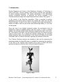
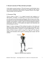
TeenSize humanoid league with a biped humanoid robot named Tulip, figure 1.1.
In the context of the RoboCup competition, TUlip is expected to perform
goalkeeping task and be able to locate a ball, dribble with it and shoot the ball
towards the goal. In order for the robot to complete these tasks successfully, it
needs to be able to walk on even terrain while maintaining stability, i.e. not to fall
on the ground.
Since the robot is an instable dynamical system, the movements must be
achieved by means of feedback position and force control. In order to maintain
stability, the controller needs actual information regarding the state of the robot.
As of the writing of this report, only the positions and force in the robots joints are
used for robot control. For a natural and dynamic walking gait, the controller
needs information about the coordinates of the robots body relative to the world
coordinate frame, as well as information regarding the pressures at the feet.
Four Tekscan Flexiforce sensors are available at each foot for measuring the
pressures present. An Xsens Mti sensor is available for measuring the orientation
of the robot in 3D. Together these sensors will be used to correct the robots
posture and help the controller steer it along the desired trajectory
Figure 1.1 TUlip
Bachelor Final Project
Accessing sensors for control of a humanoid robot
5
The objectives of this assignment are to calibrate where needed and gain access
to both Xsens and Flexiforce readings, apply the zero moment point theory to the
Flexiforce readings by determining the center of pressure for the feet and to
provide the code necessary to run the sensors on TUlip.
This reports structure consists of an overview of TUlip, some theory regarding
different ways to describe 3D orientation, and the Center of Pressure/Zero
Moment Point. The next chapter contains an overview of the Flexiforce sensors
as well as a way to access its output and calculate the CoP using this output.
The 4th chapter of the report will deal with the Xsens orientation tracker. To round
out the report, there will be a conclusion and recommendations about the
sensors.
Bachelor Final Project
Accessing sensors for control of a humanoid robot
6
2. General overview of TUlip and basic principles
In this chapter a general overview of TUlip will be given, as well the basic theory
of the centre of pressure and zero moment point; the chapter will then continue
with the theory behind three different ways to represent rotations: Euler angles,
rotation matrixes and unit quaternions.
2.1 Overview of TUlip
TUlip as shown in Figure 1.1 is a bipedal humanoid robot weighing in at
approximately 18 kilogram. It is designed to move using a dynamic walking gait,
or in other words an anthropomorphic walking gait. When moving in such a way,
the robot will move from one dynamically unstable posture to the next one using
its weight to move forward. In order to keep the robot from falling down during its
walking, cycle feedback is needed to give the controller information about the
current state of the robot, i.e. its orientation with respect to the world frame and
the force present on the feet.
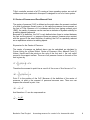
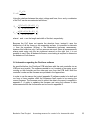
Figure 2.1 shows a drawing of TUlip including the position of the Xsens and
Flexiforce sensors. Four Flexiforce sensors are mounted at the corners of the
feet and the Xsens Module is mounted on the robot’s right shoulder. The Xsens
sensor interfaces with the controller via a serial RS-232 serial port and the
Flexiforce sensors interface with the controller via a USB hub. In the following
chapter more information will be given on interfacing these sensors with the
controller.
Figure 2.1 Tulip with sensor positions
Bachelor Final Project
Accessing sensors for control of a humanoid robot
7
TUlip’s controller consists of a PC running a Linux operating system, as such all
software and code contained in this report is designed to run on a Linux system.
2.2 Center of Pressure and Zero Moment Point
The center of pressure (CoP) is defined as the point where the moment resultant
of a field of pressures forces is zero, in this case the pressure forces present on
the feet of TUlip. Because of it’s incidence with the zero tipping moment point
(ZMP), the center of pressure can be used as an indicator of dynamic stability for
a walking bipedal humanoid.
Because of its definition, the CoP is only defined when there is contact between
the feet and the ground, i.e. pressure forces are present. However since contact
with the ground is the exact definition of walking, the CoP is a perfectly relevant
as an equilibrium criterion in walking bipeds.
Expression for the Center of Pressure:
The center of pressure as defined above can be calculated as stipulated in
Forces Acting on a Biped Robot. Center of Pressure—Zero Moment Point [1]
G
follows. Here O and P are points on the sole of the foot and n the unit vector
normal to the support surface. The sum of all pressure forces on the sole of the
feet is given by
G
⎛
⎞G
G
R p = ⎜⎜ ∫ p(P )ds ⎟⎟n = R p n
⎝s
⎠
Therefore the moment in point O as a result of the sum of the forces in P is
→
G
⎛
⎞ G
M Op = ⎜⎜ ∫ p(P )OP ds ⎟⎟ × n
⎝s
⎠
Point C is the position of the CoP. Because of the definition of the center of
pressure, at point p the moment of pressure becomes zero. Thus one can
express the moment in point O as
→
G
G
M Op = OC× R p
→
And therefore OC can be expressed as
G G
n × M Op
OC = G p
R
→
Bachelor Final Project
Accessing sensors for control of a humanoid robot
8
Incidence of the Zero tipping moment point and the CoP:
The ZMP is the point on the ground where the tipping moment due to the gravity
working on the robot and the inertia forces present equals zero. Its incidence with
the CoP can be proven as follows;
The resultant of all forces working on the robot equals the inertia force,
G
G
G
G
R p + R f + mg = ma
And the moment around a point Q equals
→
→
G →
G →
M Q = R p × QP + R f × QF + mg × QG = ma × QG
Now we define M C as the moment resultant of the contact force on the feet
and M G as the moment resultant of the gravity and inertia forces;
→
→
G
G
M QC = R p × QP + R f × QF
→
G
G
M QG = (mg − ma ) × QG
From this it follows that
M QC + M QG = 0
Now we place the point Q on the plane of the support surfaces so that the
moment in Q as a result of the friction force equals zero. Now we
obtain the following relation,
M QP + M QG = 0
Since in the CoP the moment as a result of the pressure forces M QP equals zero,
this means that in the CoP the moment resultant of the gravity and inertia forces
equals zero, thus the ZMP and CoP coincide.
2.3 Representations of 3D orientation
A rigid body’s position can be described in space by three Cartesian coordinates,
x, y, z , however such a body will still be able to rotate around the point fixed by
those parameters. To complete describe both position and orientation of a rigid
Bachelor Final Project
Accessing sensors for control of a humanoid robot
9
body, a minimum of 6 coordinates are needed, three for position and three for
orientation.
The orientation can be described in a number of different ways, however, only
three of these will be discussed in this paper; Euler angles, rotation matrices and
orientation quaternions.
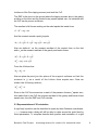
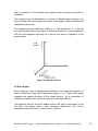
The orientation are described here relative to X O , the world frame. X O is defined
as a right-handed orthonormal frame of reference where the x axis corresponds
with the local magnetic north and the z-axis as the vector in opposition of the
gravity vector:
Figure 2.2 World frame X0
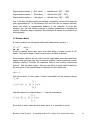
2.4 Euler Angles
Euler angles are a way to represent the orientation of an object with respect to a
frame of reference using three independent angles ϕ ,θ ,ψ . These three angles
represent the spatial orientation of the rotated frame X S as a composition of
rotations around the three axes of an orthogonal reference frame X O .
The definition used for the Euler angles used in this report is equivalent to the
roll, pitch, yaw angles used in many aerospace applications. The rotation
sequence to rotate from the X O frame to the X S frame is:
Bachelor Final Project
Accessing sensors for control of a humanoid robot
10
Right-handed rotation ϕ : Roll about xO defined from [-180º … 180º]
Right-handed rotation θ : Pitch about y O defined from [-90º … 90º]
Right-handed rotation ψ : Yaw about z O defined from [-180º … 180º]
Due to the way the Euler angles are defined a singularity occurs in the when the
pitch approaches 90º. In this situation Roll and Yaw are not uniquely defined,
which may result in unpredictable behavior of the controller; to avoid this
situation, you can use rotation matrices or rotation quaternions to describe the
rotation. These two ways to represent the orientation of a body do not suffer from
this singularity.
2.5 Rotation Matrix
A rotation matrix is an orthogonal matrix with a determinant equal to 1;
RT = R −1 ,
det( R) = 1
Rotation matrixes derive their name from their ability to rotate a vector in 3D
space. They can be used to rotate vectors from one frame to another.
Since rotation matrixes do not suffer from the singularities associated with Euler
angles, while giving an easy way to compute rotations, they’re commonly used to
describe rotations. Consider the reference frame X O and another orthonormal
frame X S with the same origin O . Now we can define a matrix which transforms
the unit vector of the original frame of reference into the rotated one
G G
R ⋅ x0 = xs
Now take a point P in the space. It can be described from the reference frame
X O as
G
⎡ x0 ⎤
G
G
G
G
p = pT x0 = [ p1 p2 p3 ] ⎢⎢ y0 ⎥⎥ = pT x0
G
⎢⎣ z0 ⎥⎦ and with respect to a rotated frame X S , it can be described as
G
⎡ xs ⎤
G
G
G
G
q = qT xs = [ q1 q2 q3 ] ⎢⎢ ys ⎥⎥ = qT xs
G
⎢⎣ zs ⎥⎦ G
G
Since both p0 and ps describe the same point it is possible to write
Bachelor Final Project
Accessing sensors for control of a humanoid robot
11
G
G
pT x0 = qT xs
G
substituting for xs gives us
G
G
pT x0 = qT ( R ⋅ x0 )
and
G G
G
G
pT x0T ⋅ x0 = qT x0T ⋅ R ⋅ x0 = qT RT
(
)
this gives us the rotation matrix R and the transformation from q to p
p = Rq.
Since the rotation matrix is orthogonal, the inverse transformation can easily be
obtained:
RT p = q.
2.6 Unit quaternion
A third way to describe rotations in 3D space is the unit quaternion, the
quaternions constitute a number system that extends the complex numbers to
four dimensions in the same way that complex numbers extends the set of real
numbers to 2 dimensions. Unit quaternions can be used to uniquely describe the
orientation of a rigid body in 3D space.
G
A unit quaternion can be interpreted as a rotation around a unit vector n by an
angle ϑ
ϑ G
ϑ ⎞
⎛
H = ⎜ cos( ), n sin( ) ⎟ , H = − H .
2
2 ⎠
⎝
Written in vector format this gives us,
G
⎡ x0 ⎤
G
z ] ⎢⎢ y0 ⎥⎥
G
⎢⎣ z0 ⎥⎦
1
G
⎛ϑ ⎞
H = ( w, x, y, z ) , w = cos ⎜ ⎟ , n =
[x y
⎛ϑ ⎞
⎝2⎠
sin ⎜ ⎟
⎝2⎠
The inverse of H is called the complex conjugate and can be calculated as
follows;
Bachelor Final Project
Accessing sensors for control of a humanoid robot
12
H * = ( w, − x, − y, − z ) = H −1.
Now take the two vectors p and q from the preceding section; now the quaternion
H transforms q to p according to the following relation,
p = HqH −1
since the product of H with its inverse equals one, the following relation can be
obtained for the inverse transformation,
H −1 pH = q.
2.7 Conversion formulae between rotation representations
The quaternions and Euler angles can be converted to a rotation matrix (and vice
versa). This section contains the relations between these three representations.
The Rotation matrix can be written in terms of the Euler angles,
⎡c(φ ) c(θ ) c(φ ) s(θ ) s(ψ ) − s(φ ) c(ψ ) c(φ ) s(θ ) c(ψ ) − s(φ ) s(ψ ) ⎤
R (φ ,θ ,ψ ) = ⎢⎢ s(φ ) c(θ ) s(φ ) s(θ ) s(ψ ) + c(φ ) s(ψ ) s(φ ) s(θ ) c(ψ ) − c(φ ) s(ψ ) ⎥⎥
⎢⎣ − s(θ )
⎥⎦
c(θ ) s(ψ )
c(θ ) s(ψ )
And in the components of the unit quaternion
⎡ 2( w2 + x 2 ) − 1 2( xy − wz )
2( xz + wy ) ⎤
⎢
⎥
R ( w, x, y, z ) = ⎢ 2( xy + wz )
2( w2 + z 2 ) − 1 2( yz − wx) ⎥ .
⎢ 2( xz − wy )
2( w2 + x 2 )
2( w2 + z 2 ) − 1⎥⎦
⎣
This gives us the following relation for the components of the unit quaternion;
1
tr ( R ) + 1
2
1
x = sgn( R32 − R23 ) R11 − R22 − R33 + 1
2
1
y = sgn( R13 − R31 ) R22 − R33 − R11 + 1
2
1
z = sgn( R21 − R12 ) R33 − R11 − R22 + 1
2
w=
Bachelor Final Project
Accessing sensors for control of a humanoid robot
13
3. Flexiforce Pressure sensors
This chapter discusses the Flexiforce sensor used to determine the CoP of the
robot. This chapter consists of an overview of the sensor, the theoretical model of
the sensor, the measurement setup used in the experiments, a section
discussing the data collected during the experiments the implementation of the
theoretical model, and a section about the software developed to run the
sensors.
As humanoid robots are inherently instable dynamical systems, it is virtually
impossible to navigate them along a desired trajectory by merely giving the
trajectory as input to the controller. Doing so would result in deviations from the
desired trajectory due to for instance disturbances from the environment and
modeling errors. These could seriously degrade the robots dynamic stability,
causing it to tip over, if no sensor feedback would be used.
As detailed in section 2.2, the dynamic stability can be represented by the ZMP.
The ZMP can be determined by measuring the CoP at the feet. By measuring
this CoP and using a negative feedback loop to correct the CoP when it is not in
a stable position, it is possible to improve the walking stability of the robot.
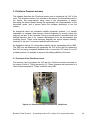
3.1 Overview of the Flexiforce sensor
The sensors used to measure the CoP are four Flexiforce sensors mounted on
the corner of both of TUlip’s feet see fig 3.2. These 4 sensors are connected to a
circuit board connected to TUlip’s controller using USB.
Figure 3.1 Flexiforce sensors mounted on Tulip’s foot
Bachelor Final Project
Accessing sensors for control of a humanoid robot
14
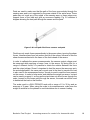
The Flexiforce sensors are composed of a thin circuit printed on a flexible film.
The sensors are resistive-based, the application of a force to the active sensing
area of the sensor results in a change in the resistance of the sensing element in
inverse proportion to the force applied, fig 3.2 shows a schematic of one of the
sensors.
Figure 4.2 Flexiforce sensor
The sensors used are of the type Sensor A201-25 which operates in the force
range through 0 to 25lbs or approximately 0 to 11 kilograms, appendix A contains
further manufacturer specifications of the sensor.
The sensor acts as a variable resistor in an electrical circuit. When the sensor is
unloaded, its resistance is very high (greater than 5 Meg-ohm); when a force is
applied to the sensor, the resistance decreases. Connecting an ohmmeter to the
outer two pins of the sensor connector and applying a force to the sensing area,
one can read the change in resistance.
Fig 3.3 shows part of the circuit used to measure the resistance of the Flexiforce
sensor.
Bachelor Final Project
Accessing sensors for control of a humanoid robot
15
Figure 3.3 Flexiforce voltage divider
Here the voltage drop over the resistor R f is measured, because this circuit works
as a voltage divider, one can use the voltage drop over the reference resistor to
determine the resistance of the sensor and thus the force applied to the sensor.
3.2 Theoretical model of the sensor
According to the schematic in fig 3.3, it’s possible to express the voltage drop:
Rf
R f + Rs
Vcc = U A
Here, R f is a reference resistor over which the voltage drop is measured,
and Rs is the resistance of the Flexiforce sensor, J5 to J8 in the figure. Since the
force applied to the sensors surface should be linear to its conductance (1/R)
according to the manufacturer [2] (see fig 3.4), it is possible to calculate the force
present on the sensor if voltage drop over the reference resistor is know.
Figure 3.4 Conductance & Resistance
Bachelor Final Project
Accessing sensors for control of a humanoid robot
16
F=
F
F+
α
Rs
α
Vcc = U A
Rf
The formulae above give the relation between the force on the sensor and the
corresponding output voltage. It is possible to rewrite these, so that the force is
expressed as a function of the output voltage;
α UA
R V
F = f cc
U
1− A
Vcc
The value of alpha can be obtained experimentally by fitting this model to a set of
measurement data obtained using the sensors.
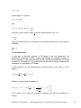
3.3 Measurement setup for the Flexiforce sensors
Fig 3.5 shows the contact area of the sensor, the entire silver area is treated as
al single contact point, for this reason it is important that the load is distributed
equally and consistently and doesn’t touch the sensor outside the silver contact
area.
Figure 3.5 Flexiforce sensor and contact area
Bachelor Final Project
Accessing sensors for control of a humanoid robot
17
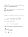
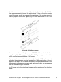
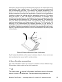
Pads are used to make sure that the path of the force goes entirely through the
sensing area and is not supported by the area outside of the active area. These
pads may not touch any of the edges of the sensing area, or these edges may
support some of the load and give an erroneous reading. Fig 3.6 contains a
diagram showing the load path through the sensor and the pads.
Figure 3.6 Load path Flexiforce sensors and pads
Flexiforce only reads forces perpendicular to the sensor plane, ignoring the shear
forces. However shear force can reduce the life of the sensor, because of this the
shear forces are directed to the frame of the feet instead of the sensor.
In order to calibrate the sensor measurements, the sensors output voltage must
be measured while applying a known force to the sensor. By doing this for a
range of different forces, it is possible to obtain the relation between the force
and the output voltage. Since it’s important to load the sensor the same way as in
the actual application, the same pad or puck used in the feed to transfer the load
is also used in the measurement setup. A scale is used to read the force present
on the sensor. In order to help center and stabilize the weight on sensor, a stand
can be used to support it, as long as the stand does not direct forces through the
scale, (except for the forces going through the sensor, the scale can still be used
to determine the load on the sensors.
The scale used is a BULLTRONICS scale with a range of 0 to 30 kg and an
accuracy of 2 gram. When using the scale to do measurements, make sure the
weight is centered on the plateau to avoid deviations due to uneven loading.
Bachelor Final Project
Accessing sensors for control of a humanoid robot
18
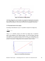
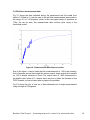
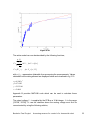
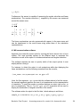
3.4 Flexiforce measurement data
Fig 3.7 shows the data collected during the experiments and the model from
section 3.2 fitted to it. It can be seen in the plot that measurements were made in
the range of 0 to 2.5 kilograms, which is also the typical range of operation on
TUlip. As can be seen, the measurement data conform quite nicely to the
theoretical model.
Figure 3.7 Measurement data fitted to model
Also in the figure, it can be seen that the measurements at 1.25 kg are missing,
this is because around that weight the sensor output stops varying and remains
on 1.65 V despite variations in force. The output value of 1.65V corresponds to
the digital output value of 0, it seems that is an error in either the firmware or the
PCB, however, we’ve not been able to pinpoint the problem.
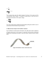
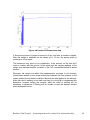
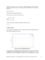
Fig 3.8 shows the plot of one set of data obtained from a single measurement
using a weight of 2 kilograms.
Bachelor Final Project
Accessing sensors for control of a humanoid robot
19
Figure 3.8 Flexiforce measurement 2kg
It shows the moment of impact at around t=2 sec, and then a number of spikes.
After the weight is stabilized on the sensor at t= 12 sec, the sensor starts to
converge to a final value.
This behaviour may prove to be problematic; if the sensors on the feet don’t
come in contact with the ground, at the same time the varying readings of the
sensor may manifest itself as a wander of the CoP coordinates around its actual
position.
Moreover, the range over which the measurements converge is not constant,
instead there seems to be a linear relationship between the force present on the
sensor and the time it takes to stabilize. Because the load applied to the sensors,
while the robot is walking, is not static over time it is not trivial to compensate this
behaviour, however testing the sensors while the robot is walking will be
necessary to determine if filtering will be needed or that the wander remains
within acceptable levels.
Bachelor Final Project
Accessing sensors for control of a humanoid robot
20
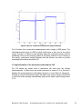
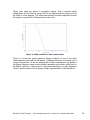
Figure 3.9 Four consecutive Flexiforce measurements
Fig 3.9 shows four consecutive measurements with a weight of 500 grams. The
standard deviation here is 0.052 kg which holds more or less true for the entire
range. Though it is difficult to say anything about the required accuracy without
knowledge of the control strategy (which is still being worked on as of writing of
this report), preliminary testing indicates that the sensors are able to provide
meaningful information about the CoP.
3.5 Implementation of the theoretical model and the CoP
Fig 3.10 shows the model used to reconstruct the force from the voltage
measurements. It differs from the model discussed in section 3.2 in the way it
handles the measurements in the higher ranges (i.e. more than five kilograms).
Instead of using the theoretical model, this part of the sensors range is linearized
to avoid the code returning unrealistically high values when output voltage nears
3.3 V.
Bachelor Final Project
Accessing sensors for control of a humanoid robot
21
Figure 3.10
The entire model can now be described by the following functions;
α UA
F=
R f Vcc
+ 0.2 , forU A = [0, x]
UA
1−
Vcc
F = βU A − γ
, for U A = [ x,3.3]
with α , β , γ , x parameters obtainable from processing the measurements. Values
obtained from the data gathered are displayed below and visualized in fig 3.10.
α = 8.5863e5
β = 97.8993
γ = 212.2146
x = 2.6869
Appendix B provides MATLAB code which can be used to calculate these
parameters.
The output voltage U A is supplied by the PCB as a 16 bit integer, U D in the range
[-32768, 32768]. To use the relations above the analog voltage must first be
reconstructed by using the following relation,
Bachelor Final Project
Accessing sensors for control of a humanoid robot
22
U A = Vcc
U D + 215
216
Using the relations between the output voltage and force, the x and y coordinates
of the CoP can be reconstructed as follows;
l ⎛ ( F + F2 ) − ( F3 + F4 ) 1 ⎞
X cop = ⎜ 1
− ⎟
2 ⎝ F1 + F2 + F3 + F4
2⎠
w ⎛ ( F + F3 ) − ( F2 + F4 ) 1 ⎞
Ycop = ⎜ 1
− ⎟,
2 ⎝ F1 + F2 + F3 + F4
2⎠
where l and w are the length and width of the feet, respectively.
Because the CoP does not require the absolute force, instead it uses the
distribution of all the forces on the supporting surface, it is possible to eliminate
α from the equations. Without α the linearization becomes unnecessary,
however this holds true only if all four sensors are equal. Since all measurements
where made using only the two rightmost sensors on the right foot, it is not
possible to say if they all behave the same, more testing is required to determine
the behaviour of all sensors.
3.6 Information regarding the Flexiforce software
As specified before, the Flexiforce PCB interfaces with the main controller via an
USB port as a joystick. The software needed to run it consists of two parts, a part
running on the controller and the other part runs from the PCB itself. Both the
controller’s code and the firmware are provided in the Appendixes.
In order to use the sensor the joytest (appendix D) software needs to be built and
run from a Linux machine while the footsensor itself needs to be running the
correct firmware. The firmware used to collect the data in the report is supplied in
appendix F. A guide to updating the firmware and using the software to take
measurements with the footsensors can be found in appendix E.
Bachelor Final Project
Accessing sensors for control of a humanoid robot
23
4. Xsens Mti Sensor Motion Tracker
This chapter will give an overview of the Xsens Mti sensor, information and
source code to communicate with the device from a Linux system as well as an
analysis of the measurements obtained with the sensor.
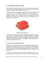
The Xsens Mti sensor is a small device capable of measuring 3D orientation data
through the use of 3D gyroscopes, accelerometers and magnetometers at a
maximum frequency of 120 Hz. The Mti sensor will be used to provide orientation
feedback to TUlip to help it maintain proper posture. Mounted on the right
shoulder of TUlip it will be able to help track the torso’s movements. Fig 4.1
shows the Xsens Mti sensor.
Figure 5.1 Xsens Mti sensor
It’s important to realize that using the data obtained with the Mti sensor to change
the orientation of the torso (by use of a negative feedback for example)
instantaneously chance the CoP-ZMP of the system (this holds true for changes
to the posture of the robot in general). The combination of the footsensors, joint
sensors and the Mti sensor provides all the feedback to TUlip Motion Control for
controlling the robot’s movement.
4.1 Overview of Xsens Mti Motion Tracker
The Mti sensor contains gyroscopes, accelerometers and magnetometers to
estimate its orientation with respect to the world frame [3]. The Mti sensor
estimates its 3D orientation with respect to the world frame by using the
measurements of the accelerometers and magnetometers to compensate for the
slowly increasing drift errors from integrating the angular velocities of the
gyroscopes.
The sensors accelerometers measure the gravitational acceleration as well as
accelerations due to movement. A filter is used to stabilize the data using the
Bachelor Final Project
Accessing sensors for control of a humanoid robot
24
assumption that the average acceleration with respect to the world frame during
some period of time is equal to zero. It’s critical for the sensor’s performance
that this assumption holds true. If for instance, the average acceleration is not
equal to zero for 20-30 seconds, the sensor’s calculated orientation starts to
deviate increasingly from the actual acceleration. However for most applications
(including a human like walking gait) this assumption holds true. The reason
being the amount of time over which the acceleration is averaged, since
according to the manufacturer’s specifications the sensor’s gyroscopes are able
to accurately track the orientation for 10-20 seconds maximum. This reduces the
time over which the assumption holds true significantly. When experiencing
significant accelerations over a large amount of time (i.e. 10 to 20 seconds), the
accuracy of the measurements will degrade depending on the amount of
acceleration, however once the average accelerations are zero again, the sensor
will stabilize. Significant accelerations over such a time period are virtually noneexistent in anthropomorphic behaviour, as such this assumption is perfectly valid
in this situation.
Figure 4.2 Xsens with sensor frame of reference
Fig 4.2 shows the definition of the sensor’s reference frame X s ; these vectors are
also inscribed on the sensor itself to avoid confusion.
4.2 Xsens Orientation representations
The Xsens Mti Motion tracker can output it’s orientation in three different ways;
Euler angles, rotation matrix and as a unit quaternion;
x0 = Rxs
The rotation matrix R , as given by the sensor, transforms a vector in the sensor
frame to a vector in the world frame. The same relation using quaternions is,
Bachelor Final Project
Accessing sensors for control of a humanoid robot
25
x0 = Hxs H −1
Furthermore, the sensor is capable of measuring its angular velocities and linear
accelerations. The angular velocities G supplied by the sensor are measured
around the sensor axes:
S = R RT
⎡ 0
⎢
S = ⎢ Sz
⎢−S y
⎣
−S z
0
Sx
Sy ⎤
⎥
−Sx ⎥ ,
0 ⎥⎦
⎡Sx ⎤
ω = ⎢⎢ S y ⎥⎥ ,
⎢⎣ S z ⎥⎦
G = RT ω
The linear accelerations are also measured with respect to the senor axes and
can be transformed to the world frame using either three of the orientation
representations.
4.3 Mti communication software
Appendix H provides the source code for running the Xsens sensor from a Linux
system. The code provides options for the different ways to represent the
orientation as well as the option to include accelerations and angular velocities.
The software requires the user to specify which of the output options it must
display before running it.
For instance, to obtain the output in unit quaternions while also displaying the
linear accelerations, run the following command from the console;
./run_xsens /dev/ttyUSB0 quat acc on gyro off Here, the first argument, /dev/ttyUSB0 tells the software where to find the sensor,
the second argument specifies the use of unit quaternions as the representation
of orientation. To use Euler angles or rotation matrixes as output, type euler or
matrix respectively. The acc on/off gyro on/off arguments can be used to
display the acceleration of angular velocities of the sensor.
The software writes its output to the file ‘data’, which makeup is as follows;
sample_nr orientation acc_x acc_y acc_z gyro_x gyro_y gyro_z Bachelor Final Project
Accessing sensors for control of a humanoid robot
26
Orientation consists of 3 to 9 columns of data dependent on which output is
chosen, using Euler angles as the output mode , the makeup of orientation becomes:
roll pitch yaw
Using the rotation matrixes it becomes:
R11 R21 R31 R12 R22 R32 R13 R23 R33 ⎡ R11
R = ⎢⎢ R21
⎢⎣ R31
R12
R22
R32
R13 ⎤
R23 ⎥⎥
R33 ⎥⎦
Finally using the unit quaternion mode the output becomes:
w x y z 4.4 Data analysis
Fig 4.3 shows a measurement of its orientation made with the Xsens Mti sensor
using the Euler angles as its output;
Figure 4.3 Xsens static measurement
As can be seen in the picture above, during the first 5 to 10 seconds the sensor
is operational it is still attempting to account for the gyroscope error. It is also
interesting to see that all angles aren’t equal to zero but instead have a small
Bachelor Final Project
Accessing sensors for control of a humanoid robot
27
offset, even when the sensor is completely steady. This is however easily
explained by the fact that the sensor itself is not aligned with its casing, but has
an offset of a few degrees. This offset can however be easily adjusted for when
the sensor is mounted in its final position on the robot.
Figure 4.4 PSD estimate of Xsens output data
Figure 4.4 shows the power spectrum density estimate of one of the static
measurements made with the Mti sensor; it displays the power of a signal over a
range of frequencies. As we are dealing with a static measurement any peaks in
the higher frequency range would indicate unwanted noise which would need to
be filtered. However, it can be seen in the picture that there is no high frequency
content, and the sensor is thus giving a ‘clean’ representation of the orientation.
Bachelor Final Project
Accessing sensors for control of a humanoid robot
28
5. Conclusion and Recommendations
With the project having run its course, it’s now possible to draw conclusions
based on the results obtained.
The goal of this project was to ‘calibrate where needed and gain access to both
Xsens and Flexiforce readings, apply the zero moment point theory to the
Flexiforce readings by determining the center of pressure for the feet and to
provide the code necessary to run the sensors on TUlip’.
These objectives have all been accomplished with both the Xsens and Flexiforce
sensor both operational and capable of running from TUlip, and calibration of the
Flexiforce sensors has been done.
While the Flexiforce sensors are now functional, some problems persist, the
possible wander of the CoP measurements because of the sensor’s initial drift as
well as the need to perform measurements on all sensors to check if there are
large deviations in behaviour between them, or if they all behave roughly the
same.
Furthermore, tests to check if the CoP measurements are accurate can be done
by placing the foot on the ground, making sure that there are no external forces
working on the feet, and then applying a single point load somewhere on the feet.
The position of this point load is the actual CoP and should coincide with the
calculated CoP. Finally, the problem of the sensors lacking any sensitivity around
1 to 1.5 kilograms must be investigated.
The Xsens Mti orientation tracker, however, provides a very clean signal and
does not require any calibration or filtering next to the internal filtering provided
by the manufacturer.
Important recommendations are to conduct experiments to find out what the
accuracy is of the CoP measurements and to investigate the necessity of
individual calibration of the Flexiforce sensors, both of these experiments were
not done over the course of this project due to unavailability of Tulip as well as
time constraints.
Finally, both the sensors’ output will have to be integrated into the motion control
of TUlip to enable it to walk properly. However the implementation of the results
obtained falls outside of the scope of this project.
Bachelor Final Project
Accessing sensors for control of a humanoid robot
29
Appendixes
A. Flexiforce manufacturer data
A201-25 Model
Physical Properties
Thickness
Width
Sensing Area
Connector
0.008" (.203mm)
0.55" (14mm)
0.375" diameter (9.53mm)
3-pin male square pin
Typical Performance
Linearity Error
Repeatability
<+/-3%
<+/-2.5% of full scale
(conditioned sensor, 80% force applied)
<4.5% of full scale
(conditioned sensor, 80% force applied)
<5% per logarithmic time scale
(constant load of 90% sensor rating)
Hysteresis
Drift
Response Time
Operating Temperatures
Force Range
Temperature Sensitivity
Bachelor Final Project
<5 microseconds
15°F to 140°F (-9°C to 60°C)
0-25 lbs. (110 N)
Output variance up to 0.2% per degree F
(approximately 0.36% per degree C)
Accessing sensors for control of a humanoid robot
30
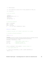
B. Matlab file for model fitting
%%%%%%%%%%%%%%%%%%%%%%%%%%%%%%%%%%%%%%%%%%%%%%%%%%%%%%%%%%%%%%%%%%%
% modelfit fits the model contained in the m file model.m to the %
% loaded data.
%
%%%%%%%%%%%%%%%%%%%%%%%%%%%%%%%%%%%%%%%%%%%%%%%%%%%%%%%%%%%%%%%%%%%
load('data2'); % load test data
%% converts loaded data to one array and converts the data's unit to kg
%test data [Sensor Output , g]'
datasum = [data0200 data0300 data0400 data0500 data0600 data0700
data0800 data0900 data1000 data1500 data1750 data2000 data2250
data2500];
% test data [kg]
datasum(2,:) = datasum(2,:)./1000;
%% find aplha wich correlates with the minimum of model(x)
alpha = fminsearch(@(x) model(x),1); % Correction factor alpha
%% Model parameters
Ud
Vcc
Rr
Dr
y
=
=
=
=
=
datasum(1,:);
3.3;
77e3;
32767;
[0:0.01:20];
%
%
%
%
%
Sensor output
[-]
voltage to sensor [V]
reference resistor [Ohm]
half of ADC range 15 bit [-]
load range 0 - 20 [kg]
%Analog voltage as a function of sensor load [V]
Ua=Vcc.*((Ud+Dr)/(2*Dr));
Uc = Vcc.*(y-.200)./(alpha/Rr+(y-.200));
%% Find the values A % B to linearize the upper end of the model
H = solve('(3.3/(alp/77000+(y-0.200))-3.3*(y-0.200)/(alp/77000+(y0.200))^2)*y+3.3-(3.3/(alp/77000+(y-0.200))-3.3*(y0.200)/(alp/77000+(y-0.200))^2)*11.3=3.3*(y-0.200)/(alp/77000+(y0.200))','y');
Bachelor Final Project
Accessing sensors for control of a humanoid robot
31
x = subs(H,alpha);
A = (Vcc/(alpha/Rr+(x-.200))-Vcc*(x-.200)/(alpha/Rr+(x-.200))^2);
B = 3.3-A*11.3;
%% plot the results
figure();
plot(datasum(2,:),Ua,'.');
hold on;
plot(y,Uc);
plot(y,A*y+B,'r');
%% Determine Parameters
Alpha
Beta
Gamma
x
=
=
=
=
9.81*alpha;
9.81/A;
B*9.81/A;
Vcc.*(x-.200)./(alpha/Rr+(x-.200));
function f = model(x)
% model(x) fits data x to a model of the from x = A* y/(y+B)
%% Load data and define parameters
load('data2');
datasum =
[data0200,data0300,data0400,data0500,data0600,data0700,data0800,data090
0,data1000,data1500,data1750,data2000,data2250,data2500];
datasum(2,:)=datasum(2,:)./1000;
Dr=32767;
Vcc=3.3;
Rf= 77e3;
% Halve digital output range [-]
% Reference voltage [V]
% Reference Resistor [R]
Ua=Vcc.*((datasum(1,:)+Dr)/(2*Dr)); % Analog voltage [V]
%% least squares model fit
f = sum((Ua-Vcc*((datasum(2,:)-.200)./((x/Rf)+(datasum(2,:).200)))).^2);
Bachelor Final Project
Accessing sensors for control of a humanoid robot
32
C. Measurement data
Flexiforce measurement data is included on the CD-ROM.
Bachelor Final Project
Accessing sensors for control of a humanoid robot
33
D. Joytest source code
Joytest source code is included on the CD-ROM.
Bachelor Final Project
Accessing sensors for control of a humanoid robot
34
E. Foot Firmware
The Foot Firmware is included on the CD-ROM.
Bachelor Final Project
Accessing sensors for control of a humanoid robot
35
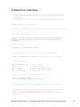
F. Guide to working with Flexiforce
Updating the firmware from the Dutch RoboCup wiki [4]:
Foot firmware can be found on the CD-ROM or alternatively from:
https://robocup.3xo.eu/ROBOCUP-3TU/ROBOCUP2008/Tulip/trunk/software/FootWare/
Though now guarantee can be given that the firmware is compatible with the
software supplied with this report.
A simple manual:
•
get Winarm from
http://www.siwawi.arubi.uni-kl.de/avr_projects/arm_projects/#winarm
•
•
•
Unzip for example to C:\Winarm
add C:\WinARM\bin;C:\WinARM\utils\bin to your system path
get Flashmagic from
http://www.flashmagictool.com/download.html&d=FlashMagic.exe
•
•
Open the footware.pnproj in Programmers Notepad, go to Tools, make all
Or (alternatively) go with a command line tool to the folder
Footware\sources and type 'make all'
Two hex-files will be generated (leftfoot.hex and rightfoot.hex) which need
to be programmed into the corresponding feet. Attach a serial cable to the
board's COM0 (5 wire serialport) (using the cable with on one end a 8-pin
micromatch and on the other end two db9-female connectors). A standard
1:1 serial cable (no crosslink) or Serial-USB cable can be used.
Check which local comport is connected (Windows hardware setup)
Startup Flashmagic, set the following settings:
•
•
•
FlashMagic settings:
Local COM: (i.e. COM3)
Baudrate: 38400
Device: LPC2148
Interface: None(ISP)
Freq: 12 MHz
•
Hit 'start'.
Bachelor Final Project
Accessing sensors for control of a humanoid robot
36
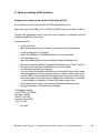
Doing measurements on TUlip
The Joytest software is currently installed on TUlip. Logging on and executing the
command ./joytest4 will start the measurement. If the joytest software is not
installed on TUlip, copy and paste the file joytest4 located on the CD-ROM into
on of TUlip’s directories. While taking calibration measurements, make sure the entire path of the force
goes through the sensing area as explained in section 3.3.
Bachelor Final Project
Accessing sensors for control of a humanoid robot
37
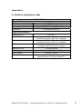
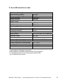
G. Xsens Mti manufacturer data Attidude and Heading
Static accuracy (roll/pitch)
Static accuracy (heading)1
Dynamic accuracy2
Angular resolution3
Dynamic range:
- Pitch
- Roll/Heading
Maximum update rate:
- Onboard processing
- External processing
Interfacing
Digital interface
Operating voltage
Power consumption
Interface options i/o
Maximum Operational limits
Ambient temperature operating range4
Specified performance operating range4
<0.5 deg
<1 deg
2 deg RMS
0.05 deg
± 90 deg
± 180 deg
120 Hz
512 Hz
RS-232, RS-485, RS 422 and USB
4,5 - 30V
350 mW
SyncOut, AnalogIn, SyncIn
-20.... +60 oC
0.... + 55 oC
1
in homogeneous magnetic environment
under condition of a stabilized Xsens sensor fusion algorithm
3
1σ standard deviation of zero-mean angular random walk
4
non-condensing environment
2
Bachelor Final Project
Accessing sensors for control of a humanoid robot
38
H. Xsens source code
Xsens Source code is included on the CD-ROM.
Bachelor Final Project
Accessing sensors for control of a humanoid robot
39
I. Sources
[1]
Philippe Sardain and Guy Bessonnet - Forces Acting on a Biped Robot.
Center of Pressure—Zero Moment Point, 2004
[2]
Tekscan - Flexiforce User manual, 2009
[3]
Xsens - MTi and MTx User Manual and Technical Documentation, 2009
[4]
http://wiki.dutchrobocup.com/Footsensors
Bachelor Final Project
Accessing sensors for control of a humanoid robot
40