Download Chaco Documentation - Enthought Tool Suite

Chaco Documentation
Release 3.0.0
Enthought
October 07, 2008
ii
CONTENTS
1
.
.
.
.
3
3
3
8
9
2
Installing and Building Chaco
2.1 Installing via EPD . . . . . . . . . . . . . . . . . . . . . . . . . . . . . . . . . . . . . . . . . . . .
2.2 easy_install . . . . . . . . . . . . . . . . . . . . . . . . . . . . . . . . . . . . . . . . . . . . . . . .
2.3 Building from Source . . . . . . . . . . . . . . . . . . . . . . . . . . . . . . . . . . . . . . . . . .
11
11
11
11
3
Tutorials
3.1 Interactive Plotting with Chaco . . . . . . . . .
3.2 Modelling Van Der Waal’s Equation With Chaco
3.3 WX-based Tutorial . . . . . . . . . . . . . . . .
3.4 Exploring Chaco with IPython . . . . . . . . . .
.
.
.
.
13
13
37
42
42
4
Architecture Overview
4.1 Core Ideas . . . . . . . . . . . . . . . . . . . . . . . . . . . . . . . . . . . . . . . . . . . . . . . .
4.2 The Relationship Between Chaco, Enable, and Kiva . . . . . . . . . . . . . . . . . . . . . . . . . .
45
45
45
5
Commonly Used Modules and Classes
5.1 Base Classes . . . . . . . . . . .
5.2 Data Objects . . . . . . . . . . .
5.3 Containers . . . . . . . . . . . .
5.4 Renderers . . . . . . . . . . . . .
5.5 Tools . . . . . . . . . . . . . . .
5.6 Overlays . . . . . . . . . . . . .
5.7 Miscellaneous . . . . . . . . . .
.
.
.
.
.
.
.
.
.
.
.
.
.
.
.
.
.
.
.
.
.
.
.
.
.
.
.
.
.
.
.
.
.
.
.
.
.
.
.
.
.
.
.
.
.
.
.
.
.
.
.
.
.
.
.
.
.
.
.
.
.
.
.
.
.
.
.
.
.
.
.
.
.
.
.
.
.
.
.
.
.
.
.
.
.
.
.
.
.
.
.
.
.
.
.
.
.
.
.
.
.
.
.
.
.
.
.
.
.
.
.
.
.
.
.
.
.
.
.
.
.
.
.
.
.
.
.
.
.
.
.
.
.
.
.
.
.
.
.
.
.
.
.
.
.
.
.
.
.
.
.
.
.
.
.
.
.
.
.
.
.
.
.
.
.
.
.
.
.
.
.
.
.
.
.
.
.
.
.
.
.
.
.
.
.
.
.
.
.
.
.
.
.
.
.
.
.
.
.
.
.
.
.
.
.
.
.
.
.
.
.
.
.
.
.
.
.
.
.
.
.
.
.
.
.
.
.
.
.
.
.
.
.
.
.
.
.
.
.
.
.
.
.
.
.
.
.
.
.
.
.
.
49
49
49
50
50
50
50
50
How Do I...?
6.1 Basics . . . . . . . . .
6.2 Layout and Rendering
6.3 Writing Components .
6.4 Advanced . . . . . . .
.
.
.
.
.
.
.
.
.
.
.
.
.
.
.
.
.
.
.
.
.
.
.
.
.
.
.
.
.
.
.
.
.
.
.
.
.
.
.
.
.
.
.
.
.
.
.
.
.
.
.
.
.
.
.
.
.
.
.
.
.
.
.
.
.
.
.
.
.
.
.
.
.
.
.
.
.
.
.
.
.
.
.
.
.
.
.
.
.
.
.
.
.
.
.
.
.
.
.
.
.
.
.
.
.
.
.
.
.
.
.
.
.
.
.
.
.
.
.
.
.
.
.
.
.
.
.
.
.
.
.
.
.
.
.
.
.
.
.
.
.
.
.
.
51
51
52
53
53
Frequently Asked Questions
7.1 Where does the name “Chaco” come from? . . . . . . . . . . . . . . . . . . . . . . . . . . . . . . .
7.2 Why was Chaco named “Chaco2” for a while? . . . . . . . . . . . . . . . . . . . . . . . . . . . . .
7.3 What are the pros and cons of Chaco vs. matplotlib? . . . . . . . . . . . . . . . . . . . . . . . . . .
55
55
55
55
6
7
Quickstart
1.1 Installation Overview . .
1.2 Running Some Examples
1.3 Creating a Plot . . . . . .
1.4 Further Reading . . . . .
.
.
.
.
.
.
.
.
.
.
.
.
.
.
.
.
.
.
.
.
.
.
.
.
.
.
.
.
.
.
.
.
.
.
.
.
.
.
.
.
.
.
.
.
.
.
.
.
.
.
.
.
.
.
.
.
.
.
.
.
.
.
.
.
.
.
.
.
.
.
.
.
.
.
.
.
.
.
.
.
.
.
.
.
.
.
.
.
.
.
.
.
.
.
.
.
.
.
.
.
.
.
.
.
.
.
.
.
.
.
.
.
.
.
.
.
.
.
.
.
.
.
.
.
.
.
.
.
.
.
.
.
.
.
.
.
.
.
.
.
.
.
.
.
.
.
.
.
.
.
.
.
.
.
.
.
.
.
.
.
.
.
.
.
.
.
.
.
.
.
.
.
.
.
.
.
.
.
.
.
.
.
.
.
.
.
.
.
.
.
.
.
.
.
.
.
.
.
.
.
.
.
.
.
.
.
.
.
.
.
.
.
.
.
.
.
.
.
.
.
.
.
.
.
.
.
.
.
.
.
.
.
.
.
.
.
.
.
.
.
.
.
.
.
.
.
.
.
.
.
.
.
.
.
.
.
.
.
.
.
.
.
.
.
.
.
.
.
.
.
.
.
.
.
.
.
.
.
.
.
.
.
.
.
.
.
.
.
i
8
9
ii
Programmer’s Reference
8.1 Data Sources . . . .
8.2 Data Ranges . . . .
8.3 Mappers . . . . . .
8.4 Containers . . . . .
.
.
.
.
.
.
.
.
.
.
.
.
.
.
.
.
.
.
.
.
.
.
.
.
.
.
.
.
.
.
.
.
.
.
.
.
.
.
.
.
.
.
.
.
.
.
.
.
.
.
.
.
.
.
.
.
.
.
.
.
.
.
.
.
.
.
.
.
.
.
.
.
.
.
.
.
.
.
.
.
.
.
.
.
.
.
.
.
.
.
.
.
.
.
.
.
.
.
.
.
.
.
.
.
.
.
.
.
.
.
.
.
59
59
65
69
71
Annotated Examples
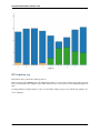
9.1 bar_plot.py . . . . . . . . . . . . . . . . . .
9.2 bigdata.py . . . . . . . . . . . . . . . . . . .
9.3 cursor_tool_demo.py . . . . . . . . . . . .
9.4 data_labels.py . . . . . . . . . . . . . . . .
9.5 data_view.py . . . . . . . . . . . . . . . . .
9.6 edit_line.py . . . . . . . . . . . . . . . . .
9.7 financial_plot.py . . . . . . . . . . . . .
9.8 financial_plot_dates.py . . . . . . . . .
9.9 multiaxis.py . . . . . . . . . . . . . . . . .
9.10 multiaxis_using_Plot.py . . . . . . . . .
9.11 noninteractive.py . . . . . . . . . . . . .
9.12 range_selection_demo.py . . . . . . . . .
9.13 scales_test.py . . . . . . . . . . . . . . . .
9.14 simple_line.py . . . . . . . . . . . . . . . .
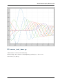
9.15 tornado.py . . . . . . . . . . . . . . . . . . .
9.16 two_plots.py . . . . . . . . . . . . . . . . .
9.17 vertical_plot.py . . . . . . . . . . . . . .
9.18 data_cube.py . . . . . . . . . . . . . . . . .
9.19 data_stream.py . . . . . . . . . . . . . . . .
9.20 scalar_image_function_inspector.py
9.21 spectrum.py . . . . . . . . . . . . . . . . . .
9.22 cmap_image_plot.py . . . . . . . . . . . . .
9.23 cmap_image_select.py . . . . . . . . . . .
9.24 cmap_scatter.py . . . . . . . . . . . . . . .
9.25 contour_cmap_plot.py . . . . . . . . . . .
9.26 contour_plot.py . . . . . . . . . . . . . . .
9.27 grid_container.py . . . . . . . . . . . . .
9.28 grid_container_aspect_ratio . . . . .
9.29 image_from_file.py . . . . . . . . . . . . .
9.30 image_inspector.py . . . . . . . . . . . . .
9.31 image_plot.py . . . . . . . . . . . . . . . . .
9.32 inset_plot.py . . . . . . . . . . . . . . . . .
9.33 line_drawing.py . . . . . . . . . . . . . . .
9.34 line_plot1.py . . . . . . . . . . . . . . . . .
9.35 line_plot_hold.py . . . . . . . . . . . . .
9.36 log_plot.py . . . . . . . . . . . . . . . . . .
9.37 nans_plot.py . . . . . . . . . . . . . . . . .
9.38 polygon_plot.py . . . . . . . . . . . . . . .
9.39 polygon_move.py . . . . . . . . . . . . . . .
9.40 regression.py . . . . . . . . . . . . . . . . .
9.41 scatter.py . . . . . . . . . . . . . . . . . . .
9.42 scatter_inspector.py . . . . . . . . . . .
9.43 scatter_select.py . . . . . . . . . . . . .
9.44 scrollbar.py . . . . . . . . . . . . . . . . .
9.45 tabbed_plots.py . . . . . . . . . . . . . . .
9.46 traits_editor.py . . . . . . . . . . . . . .
9.47 zoomable_colorbar.py . . . . . . . . . . .
.
.
.
.
.
.
.
.
.
.
.
.
.
.
.
.
.
.
.
.
.
.
.
.
.
.
.
.
.
.
.
.
.
.
.
.
.
.
.
.
.
.
.
.
.
.
.
.
.
.
.
.
.
.
.
.
.
.
.
.
.
.
.
.
.
.
.
.
.
.
.
.
.
.
.
.
.
.
.
.
.
.
.
.
.
.
.
.
.
.
.
.
.
.
.
.
.
.
.
.
.
.
.
.
.
.
.
.
.
.
.
.
.
.
.
.
.
.
.
.
.
.
.
.
.
.
.
.
.
.
.
.
.
.
.
.
.
.
.
.
.
.
.
.
.
.
.
.
.
.
.
.
.
.
.
.
.
.
.
.
.
.
.
.
.
.
.
.
.
.
.
.
.
.
.
.
.
.
.
.
.
.
.
.
.
.
.
.
.
.
.
.
.
.
.
.
.
.
.
.
.
.
.
.
.
.
.
.
.
.
.
.
.
.
.
.
.
.
.
.
.
.
.
.
.
.
.
.
.
.
.
.
.
.
.
.
.
.
.
.
.
.
.
.
.
.
.
.
.
.
.
.
.
.
.
.
.
.
.
.
.
.
.
.
.
.
.
.
.
.
.
.
.
.
.
.
.
.
.
.
.
.
.
.
.
.
.
.
.
.
.
.
.
.
.
.
.
.
.
.
.
.
.
.
.
.
.
.
.
.
.
.
.
.
.
.
.
.
.
.
.
.
.
.
.
.
.
.
.
.
.
.
.
.
.
.
.
.
.
.
.
.
.
.
.
.
.
.
.
.
.
.
.
.
.
.
.
.
.
.
.
.
.
.
.
.
.
.
.
.
.
.
.
.
.
.
.
.
.
.
.
.
.
.
.
.
.
.
.
.
.
.
.
.
.
.
.
.
.
.
.
.
.
.
.
.
.
.
.
.
.
.
.
.
.
.
.
.
.
.
.
.
.
.
.
.
.
.
.
.
.
.
.
.
.
.
.
.
.
.
.
.
.
.
.
.
.
.
.
.
.
.
.
.
.
.
.
.
.
.
.
.
.
.
.
.
.
.
.
.
.
.
.
.
.
.
.
.
.
.
.
.
.
.
.
.
.
.
.
.
.
.
.
.
.
.
.
.
.
.
.
.
.
.
.
.
.
.
.
.
.
.
.
.
.
.
.
.
.
.
.
.
.
.
.
.
.
.
.
.
.
.
.
.
.
.
.
.
.
.
.
.
.
.
.
.
.
.
.
.
.
.
.
.
.
.
.
.
.
.
.
.
.
.
.
.
.
.
.
.
.
.
.
.
.
.
.
.
.
.
.
.
.
.
.
.
.
.
.
.
.
.
.
.
.
.
.
.
.
.
.
.
.
.
.
.
.
.
.
.
.
.
.
.
.
.
.
.
.
.
.
.
.
.
.
.
.
.
.
.
.
.
.
.
.
.
.
.
.
.
.
.
.
.
.
.
.
.
.
.
.
.
.
.
.
.
.
.
.
.
.
.
.
.
.
.
.
.
.
.
.
.
.
.
.
.
.
.
.
.
.
.
.
.
.
.
.
.
.
.
.
.
.
.
.
.
.
.
.
.
.
.
.
.
.
.
.
.
.
.
.
.
.
.
.
.
.
.
.
.
.
.
.
.
.
.
.
.
.
.
.
.
.
.
.
.
.
.
.
.
.
.
.
.
.
.
.
.
.
.
.
.
.
.
.
.
.
.
.
.
.
.
.
.
.
.
.
.
.
.
.
.
.
.
.
.
.
.
.
.
.
.
.
.
.
.
.
.
.
.
.
.
.
.
.
.
.
.
.
.
.
.
.
.
.
.
.
.
.
.
.
.
.
.
.
.
.
.
.
.
.
.
.
.
.
.
.
.
.
.
.
.
.
.
.
.
.
.
.
.
.
.
.
.
.
.
.
.
.
.
.
.
.
.
.
.
.
.
.
.
.
.
.
.
.
.
.
.
.
.
.
.
.
.
.
.
.
.
.
.
.
.
.
.
.
.
.
.
.
.
.
.
.
.
.
.
.
.
.
.
.
.
.
.
.
.
.
.
.
.
.
.
.
.
.
.
.
.
.
.
.
.
.
.
.
.
.
.
.
.
.
.
.
.
.
.
.
.
.
.
.
.
.
.
.
.
.
.
.
.
.
.
.
.
.
.
.
.
.
.
.
.
.
.
.
.
.
.
.
.
.
.
.
.
.
.
.
.
.
.
.
.
.
.
.
.
.
.
.
.
.
.
.
.
.
.
.
.
.
.
.
.
.
.
.
.
.
.
.
.
.
.
.
.
.
.
.
.
.
.
.
.
.
.
.
.
.
.
.
.
.
.
.
.
.
.
.
.
.
.
.
.
.
.
.
.
.
.
.
.
.
.
.
.
.
.
.
.
.
.
.
.
.
.
.
.
.
.
.
.
.
.
.
.
.
.
.
.
.
.
.
.
.
.
.
.
.
.
.
.
.
.
.
.
.
.
.
.
.
.
.
.
.
.
.
.
.
.
.
.
.
.
.
.
.
.
.
.
.
.
.
.
.
.
.
.
.
.
.
.
.
.
.
.
.
.
.
.
.
.
.
.
.
.
.
.
.
.
.
.
.
.
.
.
.
.
.
.
.
.
.
.
.
.
.
.
.
.
.
.
.
.
.
.
.
.
.
.
.
.
.
.
.
.
.
.
.
.
.
.
.
.
.
.
.
.
.
.
.
.
.
.
.
.
.
.
.
.
.
.
.
.
.
.
.
.
.
.
.
.
.
.
.
.
.
.
.
.
.
.
.
.
.
.
.
.
.
.
.
.
.
.
.
.
.
.
.
.
.
.
.
.
.
.
.
.
.
.
.
.
.
.
.
.
.
.
.
.
.
75
75
76
77
78
79
80
81
82
83
84
85
86
87
88
89
90
91
92
93
94
95
96
97
98
99
100
101
102
103
104
105
106
107
108
109
110
110
111
112
113
114
115
116
117
118
119
120
.
.
.
.
.
.
.
.
.
.
.
.
.
.
.
.
.
.
.
.
.
.
.
.
.
.
.
.
.
.
.
.
.
.
.
.
.
.
.
.
.
.
.
.
.
.
.
.
.
.
.
.
.
.
.
.
.
.
.
.
9.48 zoomed_plot . . . . . . . . . . . . . . . . . . . . . . . . . . . . . . . . . . . . . . . . . . . . . 121
10 Tech Notes
123
10.1 About the Chaco Scales package . . . . . . . . . . . . . . . . . . . . . . . . . . . . . . . . . . . . . 123
Index
125
iii
iv
Chaco Documentation, Release 3.0.0
Chaco is a Python toolkit for building interactive 2-D visualizations. It includes renderers for many popular plot types,
built-in implementations of common interactions with those plots, and a framework for extending and customizing
plots and interactions. Chaco can also render graphics in a non-interactive fashion to images, in either raster or vector
formats, and it has a subpackage for doing command-line plotting or simple scripting.
Chaco is built on three other Enthought packages:
• Traits, as an event notification framework
• Kiva, for rendering 2-D graphics to a variety of backends across platforms
• Enable, as a framework for writing interactive visual components, and for abstracting away GUI-toolkit-specific
details of mouse and keyboard handling
Currently, Chaco requires either wxPython or PyQt to display interactive plots, but a cross-platform OpenGL backend
(using Pyglet) is in the works, and it will not require WX or Qt.
Contents
1
2
CHAPTER
ONE
Quickstart
This section is meant to help users on well-supported platforms and common Python environments get started using
Chaco as quickly as possible. If your platform is not listed here, or your Python installation has some quirks, then
some of the following instructions might not work for you. If you encounter any problems in the steps below, please
refer to the Installing and Building Chaco section for more detailed instructions.
1.1 Installation Overview
There are several different ways to get Chaco:
• Install the Enthought Python Distribution. Chaco and the rest of the Enthought Tool Suite are bundled with it.
Go to the main Enthought Python Distribution (EPD) web site and download the appropriate version for your
platform. After running the installer, you will have a working version of Chaco.
Available platforms:
– Windows 32-bit
– Mac OS X 10.4 and 10.5
– RedHat Enterprise Linux 3 (32-bit and 64-bit)
Note: Enthought Python Distribution is free for academic and personal use, and fee-based for commercial and
government use.
• (Windows, Mac) Install from PyPI using easy_install (part of setuptools) from the command line:
easy_install Chaco
• (Linux) Install distribution-specific eggs from Enthought’s repository. See the ETS wiki for instructions for
installing pre-built binary eggs for your specific distribution of Linux.
• (Linux) Install via the distribution’s packaging mechanism. We provide .debs for Debian and Ubuntu and .rpms
for Redhat. (TODO)
• Download source as tarballs or from Subversion and build. See the Installing and Building Chaco section.
Chaco requires Python version 2.5.
1.2 Running Some Examples
Depending on how you installed Chaco, you may or may not have the examples already.
If you installed Chaco as part of EPD, the location of the examples depends on your platform:
3
Chaco Documentation, Release 3.0.0
• On Windows, they are in the Examples\ subdirectory of your installation location.
C:\Python25\Examples.
This is typically
• On Linux, they are in the Examples/ subdirectory of your installation location.
• On Mac OS X, they are in the /Applications/<EPD Version>/Examples/ directory.
If you downloaded and installed Chaco from source (via the PyPI tar.gz file, or from an SVN checkout), the examples are located in the examples/ subdirectory inside the root of the Chaco source tree, next to docs/ and the
enthought/ directories.
If you installed Chaco as a binary egg from PyPI for your platform, or if you happen to be on a machine with Chaco
installed, but you don’t know the exact installation mechanism, then you will need to download the examples separately
using Subversion:
• ETS 3.0 or Chaco 3.0:
svn co https://svn.enthought.com/svn/enthought/Chaco/tags/3.0.0/examples
• ETS 2.8 or Chaco 2.0.x:
svn co https://svn.enthought.com/svn/enthought/Chaco/tags/enthought.chaco2_2.0.5/examples
Almost all of the Chaco examples are stand-alone files that can be run individually, from any location.
All of the following instructions that involve the command line assume that you are in the same directory as the
examples.
1.2.1 Command line
Run the simple_line example:
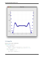
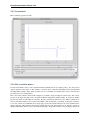
python simple_line.py
This opens a plot of several Bessel functions and a legend.
4
Contents
Chaco Documentation, Release 3.0.0
You can interact with the plot in several ways:
• To pan the plot, hold down the left mouse button inside the plot area (but not on the legend) and drag the mouse.
• To zoom the plot:
– Mouse wheel: scroll up to zoom in, and scroll down to zoom out.
– Zoom box: Press “z”, and then draw a box region to zoom in on. (There is no box-based zoom out.) Press
Ctrl-Left and Ctrl-Right to go back and forward in your zoom box history.
– Drag: hold down the right mouse button and drag the mouse up or down. Up zooms in, and down zooms
out.
– For any of the above, press Escape to resets the zoom to the original view.
• To move the legend, hold down the right mouse button inside the legend and drag it around. Note that you can
move the legend outside of the plot area.
• To exit the plot, click the “close window” button on the window frame (Windows, Linux) or choose the Quit
option on the Python menu (on Mac). Alternatively, can you press Ctrl-C in the terminal.
You can run most of the examples in the top-level examples directory, the examples/basic/ directory, and the
examples/shell/ directory. The examples/advanced/ directory has some examples that may or may not
work on your system:
Contents
5
Chaco Documentation, Release 3.0.0
• spectrum.py requires that you have PyAudio installed and a working microphone.
• data_cube.py needs to download about 7.3mb of data from the Internet the first time it is executed, so you
must have a working Internet connection. Once the data is downloaded, you can save it so you can run the
example offline in the future.
For detailed information about each built-in example, see the Annotated Examples section.
1.2.2 IPython
While all of the Chaco examples can be launched from the command line using the standard Python interpreter, if you
have IPython installed, you can poke around them in a more interactive fashion.
Chaco provides a subpackage, currently named the “Chaco Shell”, for doing command-line plotting like Matlab
or Matplotlib. The examples in the examples/shell/ directory use this subpackage, and they are particularly
amenable to exploration with IPython.
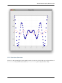
The first example we’ll look at is the lines.py example. First, we’ll run it using the standard Python interpreter:
python lines.py
This shows two overlapping line plots.
6
Contents
Chaco Documentation, Release 3.0.0
You can interact with the plot in the following ways:
• To pan the plot, hold down the left mouse button inside the plot area and dragging the mouse.
• To zoom the plot:
– Mouse wheel: scroll up zooms in, and scroll down zooms out.
– Zoom box: hold down the right mouse button, and then draw a box region to zoom in on. (There is no
box-based zoom out.) Press Ctrl-Left and Ctrl-Right to go back and forward in your zoom box history.
– For either of the above, press Escape to reset the zoom to the original view.
Now exit the plot, and start IPython with the -wthread option:
ipython -wthread
This tells IPython to start a wxPython mainloop in a background thread. Now run the previous example again:
In [1]: run lines.py
This displays the plot window, but gives you another IPython prompt. You can now use various commands from the
chaco.shell package to interact with the plot.
• Import the shell commands:
In [2]: from enthought.chaco.shell import *
• Set the X-axis title:
In [3]: xtitle("X data")
• Toggle the legend:
In [4]: legend()
After running these commands, your plot looks like this:
Contents
7
Chaco Documentation, Release 3.0.0
The chaco_commands() function display a list of commands with brief descriptions.
You can explore the Chaco object hierarchy, as well. The chaco.shell commands are just convenience functions
that wrap a rich object hierarchy that comprise the actual plot. See the Exploring Chaco with IPython section for
information on more complex and interesting things you can do with Chaco from within IPython.
1.2.3 Start Menu (MS Windows)
If you installed the Enthought Python Distribution (EPD), you have shortcuts installed in your Start Menu for many of
the Chaco examples. You can run them by just clicking the shortcut. (This just invokes python.exe on the example file
itself.)
1.3 Creating a Plot
(TODO)
8
Contents
Chaco Documentation, Release 3.0.0
1.4 Further Reading
Once you have Chaco installed, you can either visit the Tutorials to learn how to use the package, or you can run the
examples (see the Annotated Examples section).
1.4.1 Presentations
There have been several presentations on Chaco at previous PyCon and SciPy conferences. Slides and demos from
these are described below.
Currently, the examples and the scipy 2006 tutorial are the best ways to get going quickly.
http://code.enthought.com/projects/files/chaco_scipy06/chaco_talk.html)
(See
Some tutorial examples were recently added into the examples/tutorials/scipy2008/ directory on the trunk. These
examples are numbered and introduce concepts one at a time, going from a simple line plot to building a custom
overlay with its own trait editor and reusing an existing tool from the built-in set of tools. You can browse them on our
SVN server at: https://svn.enthought.com/enthought/browser/Chaco/trunk/examples/tutorials/scipy2008
1.4.2 API Docs
The API docs for Chaco 3.0 (in ETS 3.0) are at: http://code.enthought.com/projects/files/ETS3_API/enthought.chaco.html
The API docs for Chaco2 (in ETS 2.7.1) are at: http://code.enthought.com/projects/files/ets_api/enthought.chaco2.html
Contents
9
10
CHAPTER
TWO
Installing and Building Chaco
Note: (8/28/08) This section is still incomplete. For the time being, the most up-to-date information can be found on
the ETS Wiki, and, more specifically, the Install pages.
Chaco is one of the packages in the Enthought Tool Suite. It can be installed as part of ETS or as a separate package.
Even when it is installed as a standalone package, it depends on a few other packages.
2.1 Installing via EPD
Chaco and the rest of ETS are installed as part of the Enthought Python Distribution (EPD). If you have installed EPD,
then you already have Chaco!
Note: Enthought Python Distribution is free for academic and personal use, and fee-based for commercial and
government use.
2.2 easy_install
Chaco and its dependencies are available as binary eggs for Windows and Mac OS X from the Python Package Index.
Chaco depends on Numpy and either wxPython or Qt. These packages are not installed by the default installation
command. If you do not have these packages installed, use the following command to install Chaco:
easy_install Chaco[nonets]
If you do have Numpy and either wxPython or Qt installed, you can use a simpler command to install Chaco:
easy_install Chaco
Because eggs do not distinguish between various distributions of Linux, Enthought hosts its own egg repository for
Linux eggs. See the ETS wiki page on our egg repo for instructions for installing pre-built binary eggs for your specific
distribution of Linux.
For systems that don’t have binary eggs, it is also possible to build Chaco from source, since PyPI hosts the source
tarballs for all dependencies.
2.3 Building from Source
Chaco itself is not very hard to build from source; there are only a few C extensions and they build with most modern
compilers. Frequently the more difficult to build piece is actually the Enable package on which Chaco depends.
11
Chaco Documentation, Release 3.0.0
On most platforms, in order to build Enable, you need Swig > 1.3.30 and wxPython > 2.8. If you are on OS X, you
also need a recent Pyrex.
2.3.1 Obtaining the source
You can get Chaco and its dependencies from PyPI as source tarballs, or you can download the source directly from
Enthought’s Subversion server. The URL is:
https://svn.enthought.com/svn/enthought/Chaco/trunk
Note: This build instructions section is currently under construction. Please see the ETS Install From Source wiki
page for more information on building Chaco and the rest of ETS on your platform.
12
Contents
CHAPTER
THREE
Tutorials
Note: (8/28/08) This section is currently being updated to unify the information from several past presentations and
tutorials. Until it is complete, here are links to some of those. The HTML versions are built using S5, which uses
Javascript heavily. You can navigate the slide deck by using left and right arrows, as well as a drop-down box in the
lower right-hand corner.
• SciPy 2006 Tutorial (Also available in pdf)
• Pycon 2007 presentation slides
• SciPy 2008 Tutorial slides (pdf): These slides are currently being converted into the Interactive Plotting with
Chaco tutorial.
3.1 Interactive Plotting with Chaco
3.1.1 Overview
This tutorial is an introduction to Chaco. We’re going to build several mini-applications of increasing capability and
complexity. Chaco was designed to be used primarily by scientific programmers, and this tutorial only requires basic
familiarity with Python.
Knowledge of Numpy can be helpful for certain parts of the tutorial. Knowledge of GUI programming concepts such
as widgets, windows, and events are helpful for the last portion of the tutorial, but it is not required.
This tutorial will demonstrate using Chaco with Traits UI, so knowledge of the Traits framework is also helpful. We
don’t use very many sophisticated aspects of Traits or Traits UI, and it is entirely possible to pick it up as you go
through the tutorial.
It’s also worth pointing out that you don’t have to use Traits UI in order to use Chaco — you can integrate Chaco
directly with Qt or wxPython — but for this tutorial, we use Traits UI to make things easier.
13
Chaco Documentation, Release 3.0.0
Contents
• Interactive Plotting with Chaco
– Overview
– Goals
– Introduction
– Script-oriented Plotting
– Application-oriented Plotting
– Understanding the First Plot
– Scatter Plots
– Image Plot
– A Slight Modification
– Container Overview
– Using a Container
– Editing Plot Traits
3.1.2 Goals
By the end of this tutorial, you will have learned how to:
• create Chaco plots of various types
• arrange plots of data items in various layouts
• configure and interact with your plots using Traits UI
• create a custom plot overlay
• create a custom tool that interacts with the mouse
3.1.3 Introduction
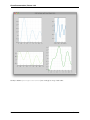
Chaco is a plotting application toolkit. This means that it can build both static plots and dynamic data visualizations
that let you interactively explore your data. Here are four basic examples of Chaco plots:
14
Contents
Chaco Documentation, Release 3.0.0
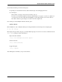
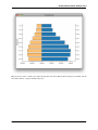
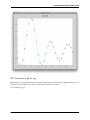
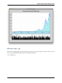
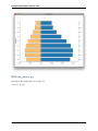
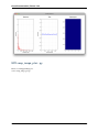
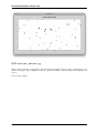
This plot shows a static “tornado plot” with a categorical Y axis and continuous X axis. The plot is resizable, but the
user cannot interact or explore the data in any way.
Contents
15
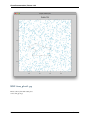
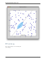
Chaco Documentation, Release 3.0.0
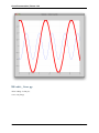
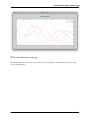
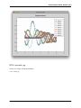
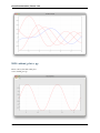
This is an overlaid composition of line and scatter plots with a legend. Unlike the previous plot, the user can pan and
zoom this plot, exploring the relationship between data curves in areas that appear densely overlapping. Furthermore,
the user can move the legend to an arbitrary position on the plot, and as they resize the plot, the legend maintains the
same screen-space separation relative to its closest corner.
16
Contents
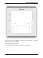
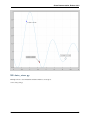
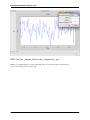
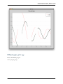
Chaco Documentation, Release 3.0.0
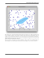
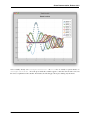
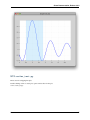
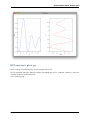
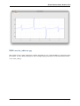
This example starts to demonstrate interacting with the dataset in an exploratory way. Whereas interactivity in the
previous example was limited to basic pan and zoom (which are fairly common in most plotting libraries), this is an
example of a more advanced interaction that allows a level of data exploration beyond the standard view manipuations.
With this example, the user can select a region of data space, and a simple line fit is applied to the selected points. The
equation of the line is then displayed in a text label.
The lasso selection tool and regression overlay are both built in to Chaco, but they serve an additional purpose of
demonstrating how one can build complex data-centric interactions and displays on top of the Chaco framework.
Contents
17
Chaco Documentation, Release 3.0.0
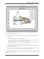
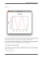
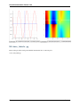
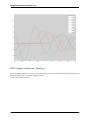
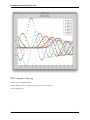
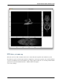
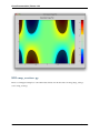
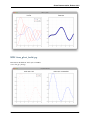
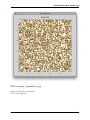
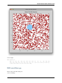
This is a much more complex demonstration of Chaco’s capabilities. The user can view the cross sections of a 2D
scalar-valued function. The cross sections update in real time as the user moves the mouse, and the “bubble” on each
line plot represents the location of the cursor along that dimension. By using drop-down menus (not show here), the
user can change plot attributes like the colormap and the number of contour levels used in the center plot, as well as
the actual function being plotted.
3.1.4 Script-oriented Plotting
We distinguish between “static” plots and “interactive visualizations” because these different applications of a library
affect the structure of how the library is written, as well as the code you write to use the library.
Here is a simple example of the “script-oriented” approach for creating a static plot. This is probably familiar to
anyone who has used Gnuplot, MATLAB, or Matplotlib:
from numpy import *
from enthought.chaco.shell import *
x = linspace(-2*pi, 2*pi, 100)
y = sin(x)
plot(x, y, "r-")
18
Contents
Chaco Documentation, Release 3.0.0
title("First plot")
ytitle("sin(x)")
show()
The basic structure of this example is that we generate some data, then we call functions to plot the data and configure
the plot. There is a global concept of “the active plot”, and the functions do high-level manipulations on it. The
generated plot is then usually saved to disk for inclusion in a journal article or presentation slides.
Now, as it so happens, this particular example uses the chaco.shell script plotting package, so when you run this script,
the plot that Chaco opens does have some basic interactivity. You can pan and zoom, and even move forwards and
backwards through your zoom history. But ultimately it’s a pretty static view into the data.
3.1.5 Application-oriented Plotting
The second approach to plotting can be thought of as “application-oriented”, for lack of a better term. There is
definitely a bit more code, and the plot initially doesn’t look much different, but it sets us up to do more interesting
things, as you’ll see later on:
class LinePlot(HasTraits):
plot = Instance(Plot)
Contents
19
Chaco Documentation, Release 3.0.0
traits_view = View(
Item(’plot’,editor=ComponentEditor(), show_label=False),
width=500, height=500, resizable=True, title="Chaco Plot")
def __init__(self):
x = linspace(-14, 14, 100)
y = sin(x) * x**3
plotdata = ArrayPlotData(x=x, y=y)
plot = Plot(plotdata)
plot.plot(("x", "y"), type="line", color="blue")
plot.title = "sin(x) * x^3"
self.plot = plot
if __name__ == "__main__":
LinePlot().configure_traits()
This produces a plot similar to the previous script-oriented code snippet:
20
Contents
Chaco Documentation, Release 3.0.0
So, this is our first “real” Chaco plot. We’ll walk through this code and look at what each bit does. This example
serves as the basis for many of the later examples.
3.1.6 Understanding the First Plot
Let’s start with the basics. First, we declare a class to represent our plot, called “LinePlot”:
class LinePlot(HasTraits):
plot = Instance(Plot)
This class uses the Enthought Traits package, and all of our objects subclass from HasTraits.
Next, we declare a Traits UI View for this class:
Contents
21
Chaco Documentation, Release 3.0.0
traits_view = View(
Item(’plot’,editor=ComponentEditor(), show_label=False),
width=500, height=500, resizable=True, title="Chaco Plot")
Inside this view, we are placing a reference to the plot trait and telling Traits UI to use the ComponentEditor to
display it. If the trait were an Int or Str or Float, Traits can automatically pick an appropriate GUI element to display
it. Since Traits UI doesn’t natively know how to display Chaco components, we explicitly tell it what kind of editor to
use.
The other parameters in the View constructor are pretty self-explanatory, and the Traits UI manual documents all the
various properties you can set here. For our purposes, this Traits View is sort of boilerplate. It gets us a nice little
window that we can resize. We’ll be using something like this View in most of the examples in the rest of the tutorial.
Now, let’s look at the constructor, where the real work gets done:
def __init__(self):
x = linspace(-14, 14, 100)
y = sin(x) * x**3
plotdata = ArrayPlotData(x=x, y=y)
The first thing we do here is create some mock data, just like in the script-oriented approach. But rather than directly
calling some sort of plotting function to throw up a plot, we create this ArrayPlotData object and stick the data in
there. The ArrayPlotData is a simple structure that associates a name with a numpy array.
In a script-oriented approach to plotting, whenever you have to update the data or tweak any part of the plot, you
basically re-run the entire script. Chaco’s model is based on having objects representing each of the little pieces of a
plot, and they all use Traits events to notify one another that some attribute has changed. So, the ArrayPlotData
is an object that interfaces your data with the rest of the objects in the plot. In a later example we’ll see how we can
use the ArrayPlotData to quickly swap data items in and out, without affecting the rest of the plot.
The next line creates an actual Plot object, and gives it the ArrayPlotData instance we created previously:
plot = Plot(plotdata)
Chaco’s Plot object serves two roles: it is both a container of renderers, which are the objects that do the actual task
of transformining data into lines and markers and colors on the screen, and it is a factory for instantiating renderers.
Once you get more familiar with Chaco, you can choose to not use the Plot object, and instead directly create renderers
and containers manually. Nonetheless, the Plot object does a lot of nice housekeeping that is useful in a large majority
of use cases.
Next, we call the plot() method on the Plot object we just created:
plot.plot(("x", "y"), type="line", color="blue")
This creates a blue line plot of the data items named “x” and “y”. Note that we are not passing in an actual array here;
we are passing in the names of arrays in the ArrayPlotData we created previously.
This method call creates a new renderer - in this case a line renderer - and adds it to the Plot.
This may seem kind of redundant or roundabout to folks who are used to passing in a pile of numpy arrays to a plot
function, but consider this: ArrayPlotData objects can be shared between multiply Plots. If you wanted several
different plots of the same data, you don’t have to externally keep track of which plots are holding on to identical copies
of what data, and then remember to shove in new data into every single one of those plots. The ArrayPlotData
acts almost like a symlink between consumers of data and the actual data itself.
Next, we set a title on the plot:
22
Contents
Chaco Documentation, Release 3.0.0
plot.title = "sin(x) * x^3"
And then we set our plot trait to the new plot:
self.plot = plot
The last thing we do in this script is set up some code to run when the script is executed:
if __name__ == "__main__":
LinePlot().configure_traits()
This one-liner instantiates a LinePlot object and calls its configure_traits method. This brings up a dialog
with a traits editor for the object, built up according to the View we created earlier. In our case, the editor will just
display our plot attribute using the ComponentEditor.
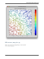
3.1.7 Scatter Plots
We can use the same pattern to build a scatter plot:
class ScatterPlot(HasTraits):
plot = Instance(Plot)
traits_view = View(
Item(’plot’,editor=ComponentEditor(), show_label=False),
width=500, height=500, resizable=True, title="Chaco Plot")
def __init__(self):
x = linspace(-14, 14, 100)
y = sin(x) * x**3
plotdata = ArrayPlotData(x = x, y = y)
plot = Plot(plotdata)
plot.plot(("x", "y"), type="scatter", color="blue")
plot.title = "sin(x) * x^3"
self.plot = plot
if __name__ == "__main__":
ScatterPlot().configure_traits()
Note that we have only changed the type argument to the plot.plot() call and the name of the object from
LinePlot to ScatterPlot. This produces the following:
Contents
23
Chaco Documentation, Release 3.0.0
3.1.8 Image Plot
Image plots can be created in a similar fashion:
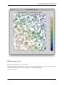
class ImagePlot(HasTraits):
plot = Instance(Plot)
traits_view = View(
Item(’plot’, editor=ComponentEditor(), show_label=False),
width=500, height=500, resizable=True, title="Chaco Plot")
def __init__(self):
x = linspace(0, 10, 50)
y = linspace(0, 5, 50)
xgrid, ygrid = meshgrid(x, y)
24
Contents
Chaco Documentation, Release 3.0.0
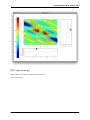
z = exp(-(xgrid*xgrid+ygrid*ygrid)/100)
plotdata = ArrayPlotData(imagedata = z)
plot = Plot(plotdata)
plot.img_plot("imagedata", xbounds=x, ybounds=y, colormap=jet)
self.plot = plot
if __name__ == "__main__":
ImagePlot().configure_traits()
There are a few more steps to create the input Z data, and we also call a different method on the Plot - img_plot()
instead of plot(). The details of the method parameters are not that important right now; this is just to demonstrate
how we can apply the same basic pattern from the “first plot” example above to do other kinds of plots.
Contents
25
Chaco Documentation, Release 3.0.0
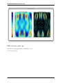
3.1.9 A Slight Modification
Earlier it was mentioned that the Plot object is both a container of renderers and a factory (or generator) of renderers.
This modification of the previous example illustrates this point. We only create a single instance of Plot, but we call
its plot() method twice. Each call creates a new renderer and adds it to the Plot‘s list of renderers. Also notice
that we are reusing the x array from the ArrayPlotData:
class OverlappingPlot(HasTraits):
plot = Instance(Plot)
traits_view = View(
Item(’plot’,editor=ComponentEditor(), show_label=False),
width=500, height=500, resizable=True, title="Chaco Plot")
def __init__(self):
x = linspace(-14, 14, 100)
y = x/2 * sin(x)
y2 = cos(x)
plotdata = ArrayPlotData(x=x, y=y, y2=y2)
plot = Plot(plotdata)
plot.plot(("x", "y"), type="scatter", color="blue")
plot.plot(("x", "y2"), type="line", color="red")
self.plot = plot
if __name__ == "__main__":
OverlappingPlot().configure_traits()
26
Contents
Chaco Documentation, Release 3.0.0
3.1.10 Container Overview
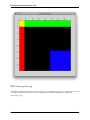
So far we’ve only seen single plots, but frequently we need to plot data side by side. Chaco uses various subclasses of
Container to do layout. Horizontal containers (HPlotContainer) place components horizontally:
Contents
27
Chaco Documentation, Release 3.0.0
Vertical containers (VPlotContainer) array component vertically:
28
Contents
Chaco Documentation, Release 3.0.0
Grid container (GridPlotContainer) lays plots out in a grid:
Contents
29
Chaco Documentation, Release 3.0.0
Overlay containers (OverlayPlotContainer) just overlay plots on top of each other:
30
Contents
Chaco Documentation, Release 3.0.0
You’ve actually already seen OverlayPlotContainer - the Plot class is actually a special subclass of
OverlayPlotContainer. All of the plots inside this container appear to share the same X and Y axis, but
this is not a requirement of the container. For instance, the following plot shows plots sharing only the X axis:
Contents
31
Chaco Documentation, Release 3.0.0
3.1.11 Using a Container
Containers can have any Chaco componeny added to them. The following code creates a separate Plot instance for
the scatter plot and the line plot, and adds them both to the HPlotContainer:
class ContainerExample(HasTraits):
plot = Instance(HPlotContainer)
traits_view = View(Item(’plot’, editor=ComponentEditor(), show_label=False),
width=1000, height=600, resizable=True, title="Chaco Plot")
def __init__(self):
x = linspace(-14, 14, 100)
y = sin(x) * x**3
plotdata = ArrayPlotData(x=x, y=y)
scatter = Plot(plotdata)
scatter.plot(("x", "y"), type="scatter", color="blue")
line = Plot(plotdata)
line.plot(("x", "y"), type="line", color="blue")
container = HPlotContainer(scatter, line)
self.plot = container
This produces the following plot:
32
Contents
Chaco Documentation, Release 3.0.0
There are many parameters you can configure on a container, like background color, border thickness, spacing, and
padding. We’re going to modify the last two lines of the previous example a little bit to make the two plots touch in
the middle:
container = HPlotContainer(scatter, line)
container.spacing = 0
scatter.padding_right = 0
line.padding_left = 0
line.y_axis.orientation = "right"
self.plot = container
Something to note here is that all Chaco components have both bounds and padding (or margin). In order to make our
plots touch, we need to zero out the padding on the appropriate side of each plot. We also move the Y axis for the line
plot (which is on the right hand side) to the right side.
This produces the following:
Contents
33
Chaco Documentation, Release 3.0.0
3.1.12 Editing Plot Traits
So far, the stuff you’ve seen is pretty standard: building up a plot of some sort and doing some layout on them. Now
we’re going to start taking advantage of the underlying framework.
Chaco is written using Traits. This means that all the graphical bits you see - and many of the bits you don’t see - are
all objects with various traits, generating events, and capable of responding to events.
We’re going to modify our previous ScatterPlot example to demonstrate some of these capabilities. Here is the full
listing of the modified code, including some of the new import lines.
from enthought.traits.api import HasTraits, Instance, Int
from enthought.enable.api import ColorTraits
from enthought.chaco.api import marker_trait
class ScatterPlotTraits(HasTraits):
plot = Instance(Plot)
color = ColorTrait("blue")
marker = marker_trait
marker_size = Int(4)
traits_view = View(
Group(Item(’color’, label="Color", style="custom"),
Item(’marker’, label="Marker"),
Item(’marker_size’, label="Size"),
Item(’plot’, editor=ComponentEditor(), show_label=False),
orientation = "vertical"),
width=800, height=600, resizable=True, title="Chaco Plot")
34
Contents
Chaco Documentation, Release 3.0.0
def __init__(self):
x = linspace(-14, 14, 100)
y = sin(x) * x**3
plotdata = ArrayPlotData(x = x, y = y)
plot = Plot(plotdata)
self.renderer = plot.plot(("x", "y"), type="scatter", color="blue")[0]
self.plot = plot
def _color_changed(self):
self.renderer.color = self.color
def _marker_changed(self):
self.renderer.marker = self.marker
def _marker_size_changed(self):
self.renderer.marker_size = self.marker_size
if __name__ == "__main__":
ScatterPlotTraits().configure_traits()
Let’s step through the changes.
First, we add traits for color, marker type, and marker size:
class ScatterPlotTraits(HasTraits):
plot = Instance(Plot)
color = ColorTrait("blue")
marker = marker_trait
marker_size = Int(4)
We’re also going to change our Traits UI View to include references to these new traits. We’ll put them in a Traits UI
Group so that we can control the layout in the dialog a little better - here, we’re setting the layout orientation of the
elements in the dialog to “vertical”.
traits_view = View(
Group(
Item(’color’, label="Color", style="custom"),
Item(’marker’, label="Marker"),
Item(’marker_size’, label="Size"),
Item(’plot’, editor=ComponentEditor(), show_label=False),
orientation = "vertical"
),
width=500, height=500, resizable=True,
title="Chaco Plot")
Now we have to do something with those traits. We’re going to modify the constructor so that we grab a handle to the
renderer that is created by the call to plot():
self.renderer = plot.plot(("x", "y"), type="scatter", color="blue")[0]
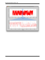
Recall that the Plot is a container for renderers and a factory for them. When called, its plot() method returns a
list of the renderers that the call created. In previous examples we’ve been just ignoring or discarding the return value,
since we had no use for it. In this case, however, we’re going to grab a reference to that renderer so that we can modify
its attributes in later methods.
Contents
35
Chaco Documentation, Release 3.0.0
The plot() method returns a list of renderers because for some values of the type argument, it will create multiple
renderers. In our case here, we are just doing a scatter plot, and this creates just a single renderer.
Next, we are going to define some Traits event handlers. These are specially-named methods that get called whenever
the value of a particular trait changes. Here is the handler for color trait:
def _color_changed(self):
self.renderer.color = self.color
This event handler gets called whenever the value of self.color changes, whether due to user interaction with a
GUI, or due to code elsewhere. (The Traits framework automatically calls this method because its name follows the
name template of “_TRAITNAME_changed”.) Since this gets called after the new value has already been updated,
we can read out the new value just by accessing self.color. We are just going to copy the color to the scatter
renderer. You can see why we needed to hold on to the renderer in the constructor.
Now we do the same thing for the marker type and marker size traits:
def _marker_changed(self):
self.renderer.marker = self.marker
def _marker_size_changed(self):
self.renderer.marker_size = self.marker_size
Running the code produces an app that looks like this:
36
Contents
Chaco Documentation, Release 3.0.0
Depending on your platform, the color editor/swatch at the top may look different. This is how it looks on Mac OS X.
All of the controls here are “live”. You can modify them and the plot will update.
3.2 Modelling Van Der Waal’s Equation With Chaco
3.2.1 Overview
This tutorial walks through the creation of an example program that plots a scientific equation. In particular, we will
model Van Der Waal’s Equation, which is a modification to the ideal gas law that takes into account the nonzero size
of molecules and the attraction to each other that they experience.
Contents
• Modelling Van Der Waal’s Equation With Chaco
– Overview
– Development Setup
– Writing the Program
– Creating the View
– Updating the Plot
– Testing your Program
– Screenshots
– But it could be better....
– Source Code
3.2.2 Development Setup
In review, Traits is a manifest typing and reactive programming package for Python. It also provides UI features that
will be used to create a simple GUI. The Traits and Traits UI user manuals are good resources for learning about the
packages and can be found on the Traits Wiki. The wiki includes features, technical notes, cookbooks, FAQ and more.
You must have Chaco and its dependencies installed:
• Traits
• TraitsGUI
• Enable
3.2.3 Writing the Program
First, define a Traits class and the elements necessary need to model the task. The following Traits class is made for the
Van Der Waal equation, whose variables can be viewed on this wiki page, Wikipedia link. The volume and pressure
variables hold lists of our X and Y coordinates, respectively, and are defined as arrays. The variables attraction and
totVolume are the input parameters specified by the user. The type of the variables as will dictate their appearance in
the GUI. For example, attraction and totVolume are defined as Ranges, so they will show up as slider bars. Likewise,
plot_type will be shown as a drop down menu since it is defined as an Enum:
Contents
37
Chaco Documentation, Release 3.0.0
# We’ll also import a few things to be used later.
from enthought.traits.api \
import HasTraits, Array, Range, Float, Enum, on_trait_change, Property
from enthought.traits.ui.api import View, Item
from enthought.chaco.chaco_plot_editor import ChacoPlotItem
from numpy import arange
class Data(HasTraits):
volume = Array
pressure = Array
attraction = Range(low=-50.0,high=50.0,value=0.0)
totVolume = Range(low=.01,high=100.0,value=0.01)
temperature = Range(low=-50.0,high=50.0,value=50.0)
r_constant= Float(8.314472)
plot_type = Enum("line", "scatter")
....
3.2.4 Creating the View
The main GUI window is created by defining a Traits View instance. This View contains all of the GUI elements,
including the plot. To link a variable with a widget element on the GUI, we create a Traits Item instance with the same
name as the variable and pass it as an argument of the Traits View instance declaration. The Traits UI user manual
discusses the View and Item objects in depth. In order to embed a Chaco plot into a Traits View, you need to import
the ChacoPlotItem, which can be passed as a parameter to View just like a the Item objects. The first two arguments
to ChacoPlotItem are the lists of X and Y coordinates for the graph. The variables volume and pressure hold the lists
of X and Y coordinates, and therefore are the first two arguments to the Chaco2PlotItem. Other parameters have been
provided to the plot for additional customization:
class Data(HasTraits):
....
traits_view = View(ChacoPlotItem("volume", "pressure",
type_trait="plot_type",
resizable=True,
x_label="Volume",
y_label="Pressure",
x_bounds=(-10,120),
x_auto=False,
y_bounds=(-2000,4000),
y_auto=False,
color="blue",
bgcolor="white",
border_visible=True,
border_width=1,
title=’Pressure vs. Volume’,
padding_bg_color="lightgray"),
Item(name=’attraction’),
Item(name=’totVolume’),
Item(name=’temperature’),
Item(name=’r_constant’, style=’readonly’),
Item(name=’plot_type’),
resizable = True,
buttons = ["OK"],
title=’Van der waal Equation’,
38
Contents
Chaco Documentation, Release 3.0.0
width=900, height=800)
....
3.2.5 Updating the Plot
The power of Traits and Chaco enable the plot to update itself whenever the X or Y arrays are changed. So, we need
a function to re-calculate the X and Y coordinate lists whenever the input parameters are changed by the user moving
the sliders in the GUI.
The volume variable is the independent variable and pressure is the dependent variable. The relationship between
pressure and volume, as derived from the equation found on the wiki page, is:
Pressure =
r_constant * Temperature
-----------------------Volume - totVolume
-
attraction
---------Volume**2
Next, there are two programing tasks to complete,
1. Define trait listener methods for your input parameters. These methods should be automatically called whenever
the parameters are changed since it will be time to recalculate the pressure array.
2. Write a calculation method that will update your lists of X and Y coordinates for your plot.
The following is the code for these two needs:
# Re-calculate when attraction, totVolume, or temperature are changed.
@on_trait_change(’attraction, totVolume, temperature’)
def calc(self):
""" Update the data based on the numbers specified by the user. """
self.volume = arange(.1, 100)
self.pressure = ((self.r_constant*self.temperature)
/(self.volume - self.totVolume)
-(self.attraction/(self.volume*self.volume)))
return
The calc() function computes the pressure array using the current values of the independent variables. Meanwhile, the
@on_trait_change() decorator (provided by Traits) tells Python to call calc() whenever any of the variables attraction,
totVolume, or temperature change.
3.2.6 Testing your Program
The application is complete, and can be tested by instantiating a copy of the class and then creating the view by calling
the configure_traits() method on the class. For a simple test, run these lines from an interpreter or a separate module:
from vanderwaals import Data
viewer = Data()
viewer.calc()
# Must calculate the initial (x,y) lists
viewer.configure_traits()
Clicking and dragging on the sliders in the GUI will dynamically update the pressure data array, and cause the plot to
update, showing the new values.
Contents
39
Chaco Documentation, Release 3.0.0
3.2.7 Screenshots
Here is what the program looks like:
3.2.8 But it could be better....
It seems inconvenient to have to call a calculation function manually before we configure_traits(). Also, the pressure
equation depends on the values of other variables, it would be nice to make the relationship between the dependant
and independent variables clearer. There is another way we could define our variables that is easier for the user, and
provides better source documentation.
Since our X values remain constant in this example it is wasteful to keep recreating the volume array. The Y array,
pressure, is the single array that needs to be updated when the independent variables change. So, instead of defining
pressure as an Array, we will define it as a Property. Property is a Traits type that allows you to define a variable whose
value is recalculated whenever it is requested. In addition, when the depends_on argument of a Property constructor
is set to list of traits in your HasTraits class, the property’s trait events will fire whenever any of the dependent trait’s
change events fire. This means that the pressure variable will fire a trait change whenever our depends_on traits are
changed. Meanwhile, the Chaco plot is automatically listening to the pressure variable, so the plot display will get the
40
Contents
Chaco Documentation, Release 3.0.0
new value of pressure whenever someone changes the input parameters!
When the value of a Property trait is requested, the _get_<trait_name>() method is called to calculate and return its
current value, so we define use the _get_pressure() method as our new calculation method. It is important to note that
this implementation does have a weakness. Since we are calculating new pressures each time someone changes the
value of the input variables, this could slow down the program if your calculation is long. When the user drags a slider
widget, each stopping point along the slider will request a recompute.
For the new implementation, these are the necessary changes:
1. Define the Y coordinate array variable as a Property instead of an Array.
2. Perform the calculations in the _get_<trait>() method for the Y coordinate array variable, which will be
_get_pressure() in this example.
3. Define the _<trait>_default() method to set the initial value of the X coordinate array so _get_pressure() does
not have to keep recalculating it.
4. Remove the previous @on_trait_change() decorator and calculation method.
The new pieces of code to add to the Data class are:
class Data(HasTraits):
...
pressure = Property(Array, depends_on=[’temperature’,
’attraction’,
’totVolume’])
...
def _volume_default(self):
return arange(.1, 100)
# Pressure is recalculated whenever one of the elements the property
# depends on changes. No need to use @on_trait_change.
def _get_pressure(self):
return ((self.r_constant*self.temperature)
/(self.volume - self.totVolume)
-(self.attraction/(self.volume*self.volume)))
You now no longer have to call an inconvenient calculation function before the first call to configure_traits()!
3.2.9 Source Code
The final version on the program, vanderwaals.py:
from enthought.traits.api \
import HasTraits, Array, Range, Float, Enum, on_trait_change, Property
from enthought.traits.ui.api import View, Item
from enthought.chaco.chaco_plot_editor import ChacoPlotItem
from numpy import arange
class Data(HasTraits):
volume = Array
pressure = Property(Array, depends_on=[’temperature’, ’attraction’,
’totVolume’])
attraction = Range(low=-50.0,high=50.0,value=0.0)
totVolume = Range(low=.01,high=100.0,value=0.01)
Contents
41
Chaco Documentation, Release 3.0.0
temperature = Range(low=-50.0,high=50.0,value=50.0)
r_constant= Float(8.314472)
plot_type = Enum("line", "scatter")
traits_view = View(ChacoPlotItem("volume", "pressure",
type_trait="plot_type",
resizable=True,
x_label="Volume",
y_label="Pressure",
x_bounds=(-10,120),
x_auto=False,
y_bounds=(-2000,4000),
y_auto=False,
color="blue",
bgcolor="white",
border_visible=True,
border_width=1,
title=’Pressure vs. Volume’,
padding_bg_color="lightgray"),
Item(name=’attraction’),
Item(name=’totVolume’),
Item(name=’temperature’),
Item(name=’r_constant’, style=’readonly’),
Item(name=’plot_type’),
resizable = True,
buttons = ["OK"],
title=’Van der waal Equation’,
width=900, height=800)
def _volume_default(self):
""" Default handler for volume Trait Array. """
return arange(.1, 100)
def _get_pressure(self):
"""Recalculate when one a trait the property depends on changes."""
return ((self.r_constant*self.temperature)
/(self.volume - self.totVolume)
-(self.attraction/(self.volume*self.volume)))
if __name__ == ’__main__’:
viewer = Data()
viewer.configure_traits()
3.3 WX-based Tutorial
3.4 Exploring Chaco with IPython
There are several tutorials for Chaco, each covering slightly different aspects:
1. Tutorial 1, Interactive Plotting with Chaco, introduces some basic concepts of how to use Chaco and Traits UI
to do basic plots, customize layout, and add interactivity.
Although Traits UI is not required to use Chaco, it is the by far the most common usage of Chaco. It is a good
approach for those who are relatively new to developing GUI applications. Using Chaco with Traits UI allows
42
Contents
Chaco Documentation, Release 3.0.0
the scientist or novice programmer to easily develop plotting applications, but it also provides them room to
grow as their requirements change and increase in complexity.
Traits UI can also be used by a more experienced developer to build more involved applications, and Chaco can
be used to embed visualizations or to leverage interactive graphs as controllers for an application.
2. Tutorial 2, Modelling Van Der Waal’s Equation With Chaco, is another example of creating a data model and
then using Traits and Chaco to rapidly create interactive plot GUIs.
3. WX-based Tutorial: Creating a stand-alone wxPython application, or embedding a Chaco plot within an existing
Wx application.
This tutorial is suited for those who are familiar with programming using wxPython or Qt and prefer to write
directly to those toolkits. It shows how to embed Chaco components directly into an enclosing widget, panel, or
dialog. It also demonstrates more advanced usages like using a wxPython Timer to display live, updating data
streams.
4. Using the Chaco Shell command-line plotting interface to build plots, in a Matlab or gnuplot-like style. Although
this approach doesn’t lend itself to building more reusable utilities or applications, it can be a quick way to get
plots on the screen and build one-off visualizations. See Exploring Chaco with IPython.
Contents
43
44
CHAPTER
FOUR
Architecture Overview
Note: At this time, this is an overview of not just Chaco, but also Kiva and Enable.
4.1 Core Ideas
The Chaco toolkit is defined by a few core architectural ideas:
• Plots are compositions of visual components
Everything you see in a plot is some sort of graphical widget, with position, shape, and appearance attributes,
and with an opportunity to respond to events.
• Separation between data and screen space
Although everything in a plot eventually ends up rendering into a common visual area, there are aspects of
the plot which are intrinsically screen-space, and some which are fundamentally data-space. Preserving the
distinction between these two domains allows us to think about visualizations in a structured way.
• Modular design and extensible classes
Chaco is meant to be used for writing tools and applications, and code reuse and good class design are important.
We use the math behind the data and visualizations to give us architectural direction and conceptual modularity.
The Traits framework allows us to use events to couple disjoint components at another level of modularity.
Also, rather than building super-flexible core objects with myriad configuration attributes, Chaco’s classes are
written with subclassing in mind. While they are certainly configurable, the classes themselves are written in a
modular way so that subclasses can easily customize particular aspects of a visual component’s appearance or a
tool’s behavior.
4.2 The Relationship Between Chaco, Enable, and Kiva
Chaco, Enable, and Kiva are three packages in the Enthought Tool Suite. They have been there for a long time now,
since almost the beginning of Enthought as a company. Enthought has delivered many applications using these toolkits.
The Kiva and Enable packages are bundled together in the “Enable” project.
4.2.1 Kiva
Kiva is a 2-D vector drawing library for Python. It serves a purpose similar to Cairo. It allows us to compose
vector graphics for display on the screen or for saving to a variety of vector and image file formats. To use Kiva, a
program instantiates a Kiva GraphicsContext object of an appropriate type, and then makes drawing calls on it like
gc.draw_image(), gc.line_to(), and gc.show_text(). Kiva integrates with windowing toolkits like wxWindows and Qt,
45
Chaco Documentation, Release 3.0.0
and it has an OpenGL backend as well. For wxPython and Qt, Kiva actually performs a high-quality, fast software
rasterization using the Anti-Grain Geometry (AGG) library. For OpenGL, Kiva has a python extension that makes
native OpenGL calls from C++.
Kiva provides a GraphicsContext for drawing onto the screen or saving out to disk, but it provides no mechanism for
user input and control. For this “control” layer, it would be convenient to have to write only one set of event callbacks
or handlers for all the platforms we support, and all the toolkits on each platform. Enable provides this layer. It
insulates all the rendering and event handling code in Chaco from the minutiae of each GUI toolkit. Additionally,
and to some extent more importantly, Enable defines the concept of “components” and “containers” that form the
foundation of Chaco’s architecture. In the Enable model, the top-most Window object is responsible for dispatching
events and drawing a single component. Usually, this component is a container with other containers and components
inside it. The container can perform layout on its internal components, and it controls how events are subsequently
dispatched to its set of components.
4.2.2 Enable
Almost every graphical component in Chaco is an instance of an Enable component or container. We’re currently
trying to push more of the layout system (implemented as the various different kinds of Chaco plot containers) down
into Enable, but as things currently stand, you have to use Chaco containers if you want to get layout. The general
trend has been that we implement some nifty new thing in Chaco, and then realize that it is a more general tool or
overlay that will be useful for other non-plotting visual applications. We then move it into Enable, and if there are
plotting-specific aspects of it, we will create an appropriate subclass in Chaco to encapsulate that behavior.
The sorts of applications that can and should be done at the Enable level include things like a visual programming
canvas or a vector drawing tool. There is nothing at the Enable level that understands the concept of mapping between
a data space to screen space and vice versa. Although there has been some debate about the incorporating rudimentary
mapping into Enable, for the time being, if you want some kind of canvas-like thing to model more than just pixel
space on the screen, implement it using the mechanisms in Chaco.
The way that Enable hooks up to the underlying GUI toolkit system is via an enable.Window object. Each toolkit
has its own implementation of this object, and they all subclass from enable.AbstractWindow. They usually
contain an instance of the GUI toolkit’s specific window object, whether it’s a wx.Window or Qt.QWidget or
pyglet.window.Window. This instance is created upon initialization of the enable.Window and stored as the
control attribute on the Enable window. From the perspective of the GUI toolkit, an opaque widget gets created
and stuck inside a parent control (or dialog or frame or window). This instance serves as a proxy between the GUI
toolkit and the world of Enable. When the user clicks inside the widget area, the control widget calls a method
on the enable.Window object, which then in turn can dispatch the event down the stack of Enable containers and
components. When the system tells the widget to draw itself (e.g., as the result of a PAINT or EXPOSE event from the
OS), the enable.Window is responsible for creating an appropriate Kiva GraphicsContext (GC), then passing it down
through the object hierarchy so that everyone gets a chance to draw. After all the components have drawn onto the
GC, for the AGG-based bitmap backends, the enable.Window object is responsible for blitting the rastered off-screen
buffer of the GC into the actual widget’s space on the screen. (For Kiva’s OpenGL backend, there is no final blit, since
calls to the GC render in immediate mode in the window’s active OpenGL context, but the idea is the same, and the
enable.Window object does perform initialization on the GL GraphicsContext.)
Some of the advantages to using Enable are that it makes mouse and key events from disparate windowing systems all
share the same kind of signature, and be accessible via the same name. So, if you write bare wxPython and handle a
key_pressed event in wx, this might generate a value of wx.WXK_BACK. Using Enable, you would just get a “key”
back and its value would be the string “Backspace”, and this would hold true on Qt4 and Pyglet. Almost all of the
event handling and rendering code in Chaco is identical under all of the backends; there are very few backend-specific
changes that need to be handled at the Chaco level.
The enable.Window object has a reference to a single top-level graphical component (which includes containers, since
they are subclasses of component). Whenever it gets user input events, it recursively dispatches all the way down the
potentially-nested stack of components. Whenever a components wants to signal that it needs to be redrawn, it calls
self.request_redraw(), which ultimately reaches the enable.Window, which can then make sure it schedules a PAINT
46
Contents
Chaco Documentation, Release 3.0.0
event with the OS. The nice thing about having the enable.Window object between the GUI toolkits and our apps, and
sitting at the very top of event dispatch, is that we can easily interject new kinds of events; this is precisely what we
did to enable all of our tools to work with Multitouch.
The basic things to remember about Enable are that:
• Any place that your GUI toolkit allows you stick a generic widget, you can stick an Enable component (and
this extends to Chaco components, as well). Dave Morrill had a neat demonstration of this by embedding small
Chaco plots as cells in a wx Table control.
• If you have some new GUI toolkit, and you want to provide an Enable backend for it, all you have to do is
implement a new Window class for that backend. You also need to make sure that Kiva can actually create a
GraphicsContext for that toolkit. Once the kiva_gl branch is committed to the trunk, Kiva will be able to render
into any GL context. So if your newfangled unsupported GUI toolkit has a GLWindow type of thing, then you
will be able to use Kiva, Enable, and Chaco inside it. This is a pretty major improvement to interoperability, if
only because users now don’t have to download and install wxPython just to play with Chaco.
4.2.3 Chaco
At the highest level, Chaco consists of:
• Visual components that render to screen or an output device (e.g., LinePlot, ScatterPlot, PlotGrid,
PlotAxis, Legend)
• Data handling classes that wrap input data, interface with application-specific data sources, and transform coordinates between data and screen space (e.g., ArrayDataSource, GridDataSource, LinearMapper)
• Tools that handle keyboard or mouse events and modify other components (e.g., PanTool, ZoomTool,
ScatterInspector)
Contents
47
48
CHAPTER
FIVE
Commonly Used Modules and Classes
5.1 Base Classes
Plot Component
All visual components in Chaco subclass from PlotComponent. It defines all of the common visual attributes like
background color, border styles and color, and whether the component is visible. (Actually, most of these visual
attributes are inherited from the Enable drawing framework.) More importantly, it provides the base behaviors for
participating in layout, handling event dispatch to tools and overlays, and drawing various layers in the correct order.
Subclasses almost never need to override or customize these base behaviors, but if they do, there are several easy
extension points.
5.2 Data Objects
5.2.1 Data Source
A data source is a wrapper object for the actual data that it will be handling. It provides methods for retrieving
data, estimating a size of the dataset, indications about the dimensionality of the data, a place for metadata (such as
selections and annotations), and events that fire when the data gets changed. There are two primary reasons for a data
source class:
• It provides a way for different plotting objects to reference the same data.
• It defines the interface for embedding Chaco into an existing application. In most cases, the standard ArrayDataSource will suffice.
Interface: AbstractDataSource
Subclasses:
ArrayDataSource,
GridDataSource, ImageData
MultiArrayDataSource,
PointDataSource,
5.2.2 Data Range
A data range expresses bounds on data space of some dimensionality. The simplest data range is just a set of two
scalars representing (low, high) bounds in 1-D. One of the important aspects of DataRanges is that their bounds can
be set to auto, which means that they automatically scale to fit their associated datasources. (Each DataSource can
be associated with multiple ranges, and each DataRange can be associated with multiple datasources.)
Interface: AbstractDataRange
49
Chaco Documentation, Release 3.0.0
Subclasses: BaseDataRange, DataRange1D, DataRange2D
5.2.3 Mapper
Mappers perform the job of mapping a data space region to screen space, and vice versa.
Interface: AbstractMapper
Subclasses: Base1DMapper, LinearMapper, LogMapper, GridMapper, PolarMapper
5.3 Containers
5.3.1 PlotContainer
PlotContainers are Chaco’s way of handling layout. Because they logically partition the screen space, they also serve as
a way for efficient event dispatch. They are very similar to sizers or layout grids in GUI toolkits like WX. Containers
are subclasses of PlotComponent, thus allowing them to be nested. BasePlotContainer implements the
logic to correctly render and dispatch events to sub-components, while its subclasses implement the different layout
calculations. Chaco currently has three types of containers, described in the following sections.
Interface: BasePlotContainer
Subclasses:
OverlayPlotContainer,
GridPlotContainer
HPlotContainer,
VPlotContainer,
5.4 Renderers
5.5 Tools
5.6 Overlays
5.7 Miscellaneous
50
Contents
CHAPTER
SIX
How Do I...?
Note: This section is currently under active development.
6.1 Basics
How do I...
• render data to an image file?:
def save_plot(plot, filename, width, height):
plot.outer_bounds = [width, height]
plot.do_layout(force=True)
gc = PlotGraphicsContext(size, dpi=72)
gc.render_component((width, height))
gc.save(filename)
• render data to screen?
• integrate a Chaco plot into my WX app?
• integrate a Chaco plot into my Traits UI?:
import numpy
from enthought.chaco.api import Plot, ArrayPlotData
from enthought.enable.enable_component import EnableComponent
from enthought.traits.api import HasTraits, Instance
from enthought.traits.ui.api import Item, View
class MyPlot(HasTraits):
plot = Instance(Plot)
traits_view = View(Item(’plot’, editor=ComponentEditor()))
def __init__(self, index, data_series, **kw):
super(MyPlot, self).__init__(**kw)
plot_data = ArrayPlotData(index=index)
plot_data.set_data(’data_series’, data_series)
self.plot = Plot(plot_data)
self.plot.plot((’index’, ’data_series’))
index = numpy.array([1,2,3,4,5])
51
Chaco Documentation, Release 3.0.0
data_series = index**2
my_plot = MyPlot(index, data_series)
my_plot.configure_traits()
• make an application to render many streams of data?:
def plot_several_series(index, series_list):
plot_data = ArrayPlotData(index=index)
plot = Plot(plot_data)
for i, data_series in enumerate(series_list):
series_name = "series_%d" % i
plot_data.set_data(series_name, data_series)
plot.plot((’index’, series_name))
• make a plot the right size?:
def resize_plot(plot, width, height):
plot.outer_bounds = [width, height]
• copy a plot the the clipboard?:
def copy_to_clipboard(plot):
# WX specific, though QT implementation is similar using
# QImage and QClipboard
import wx
width, height = plot.outer_bounds
gc = PlotGraphicsContext((width, height), dpi=72)
gc.render_component(plot_component)
# Create a bitmap the same size as the plot
# and copy the plot data to it
bitmap = wx.BitmapFromBufferRGBA(width+1, height+1,
gc.bmp_array.flatten())
data = wx.BitmapDataObject()
data.SetBitmap(bitmap)
if wx.TheClipboard.Open():
wx.TheClipboard.SetData(data)
wx.TheClipboard.Close()
else:
wx.MessageBox("Unable to open the clipboard.", "Error")
6.2 Layout and Rendering
How do I...
• put multiple plots in a single window?
• change the background color?:
52
Contents
Chaco Documentation, Release 3.0.0
def make_black_plot(index, data_series):
plot_data = ArrayPlotData(index=index)
plot_data.set_data(’data_series’, data_series)
plot = Plot(plot_data, bgcolor=’black’)
plot.plot((’index’, ’data_series’))
def change_bgcolor(plot):
plot.bgcolor = ’black’
• turn off borders?
def make_borderless_plot(index, data_series):
plot_data = ArrayPlotData(index=index)
plot_data.set_data(’data_series’, data_series)
plot = Plot(plot_data, border_visible=False)
plot.plot((’index’, ’data_series’))
def change_to_borderless_plot(plot):
plot.border_visible = False
6.3 Writing Components
How do I...
• compose multiple renderers?
• write a custom renderer?
• write a custom overlay/underlay?
• write a custom tool?
• write a new container?
6.4 Advanced
How do I...
• properly change/override draw dispatch?
• modify event dispatch?
• customize backbuffering?
• embed custom/native WX widgets on the plot?
Contents
53
54
CHAPTER
SEVEN
Frequently Asked Questions
7.1 Where does the name “Chaco” come from?
It is named after Chaco Canyon, which had astronomical markings that served as an observatory for Native Americans.
The original version of Chaco was built as part of a project for the Space Telescope Science Institute. This is also the
origin of the name “Kiva” for our vector graphics layer that Chaco uses for rendering.
7.2 Why was Chaco named “Chaco2” for a while?
Starting in January of 2006, we refactored and reimplemented much of the core Chaco API. The effort has been named
“chaco2”, and lives in the enthought.chaco2 namespace. During that time, the original Chaco package (“Chaco
Classic”) was in maintenance-only mode, but there was still code that needed features from both Chaco Classic and
Chaco2. That code has finally been either shelved or refactored, and the latest versions of Chaco (3.0 and up) are back
to residing in the enthought.chaco namespace. We still have compatibility modules in enthought.chaco2,
but they just proxy for the real code in enthought.chaco.
The same applies to the enthought.enable and enthought.enable2 packages.
7.3 What are the pros and cons of Chaco vs. matplotlib?
This question comes up quite a bit. The bottom line is that the two projects initially set out to do different things,
and although each project has grown a lot of overlapping features, the different original charters are reflected in the
capabilities and feature sets of the two projects.
Here is an excerpt from a thread about this question on the enthought-dev mailing list.
Gael Varoquaux’s response:
On Fri, May 11, 2007 at 10:03:21PM +0900, Bill Baxter wrote:
> Just curious.
What are the pros and cons of chaco vs matplotlib?
To me it seem the big pro of chaco is that it is much easier to use in a
"programatic way" (I have no clue this means something in English). It is
fully traited and rely quite a lot on inversion of control (sorry, I love
this concept, so it has become my new buzz-word). You can make very nice
object oriented interactive code.
Another nice aspect is that it is much faster than MPL.
55
Chaco Documentation, Release 3.0.0
The cons are that it is not as fully featured as MPL, that it does not
has an as nice interactively useable functional interface (ie chaco.shell
vs pylab) and that it is not as well documented and does not have the
same huge community.
I would say that the codebase of chaco is nicer, but than if you are not
developping interactive application, it is MPL is currently an option
that is lickely to get you where you want to go quicker. Not that I
wouldn’t like to see chaco building up a bit more and becoming **the** reference.
Developers, if you want chaco to pick up momentum, give it a pylab-like
interface (as close as you can to pylab) !
My 2 cents,
Gael
Peter Wang’s response (excerpt):
On May 11, 2007, at 8:03 AM, Bill Baxter wrote:
> Just curious.
What are the pros and cons of chaco vs matplotlib?
You had to go and ask, didn’t you? :) There are many more folks here
who have used MPL more extensively than myself, so I’ll defer the
comparisons to them. (Gael, as always, thanks for your comments and
feedback!) I can comment, however, on the key goals of Chaco.
Chaco is a plotting toolkit targeted towards developers for building
interactive visualizations. You hook up pieces to build a plot that
is then easy to inspect, interact with, add configuration UIs for
(using Traits UI), etc. The layout of plot areas, the multiplicity
and types of renderers within those windows, the appearance and
locations of axes, etc. are all completely configurable since these
are all first-class objects participating in a visual canvas. They
can all receive mouse and keyboard events, and it’s easy to subclass
them (or attach tools to them) to achieve new kinds of behavior.
We’ve tried to make all the plot renderers adhere to a standard
interface, so that tools and interactors can easily inspect data and
map between screen space and data space. Once these are all hooked
up, you can swap out or update the data independently of the plots.
One of the downsides we had a for a while was that this rich set of
objects required the programmer to put several different classes
together just to make a basic plot. To solve this problem, we’ve
assembled some higher-level classes that have the most common
behaviors built-in by default, but which can still be easily
customized or extended. It’s clear to me that this is a good general
approach to preserving flexibility while reducing verbosity.
At this point, Chaco is definitely capable of handling a large number
of different plotting tasks, and a lot of them don’t require too much
typing or hacking skills. (Folks will probably require more
documentation, however, but I’m working on that. :) I linked to the
source for all of the screenshots in the gallery to demonstrate that
you can do a lot of things with Chaco in a few dozen lines of code.
(For instance, the audio spectrogram at the bottom of the gallery is
just a little over 100 lines.)
56
Contents
Chaco Documentation, Release 3.0.0
Fundamentally, I like the Chaco model of plots as compositions of
interactive components. This really helps me think about
visualization apps in a modular way, and it "fits my head". (Of
course, the fact that I wrote much of it might have something to do
with that as well. ;) The goal is to have data-related operations
clearly happen in one set of objects, the view layout and
configuration happen in another, and the interaction controls fit
neatly into a third. IMHO a good toolkit should help me design/
architect my application better, and we definitely aspire to make
Chaco meet that criterion.
Finally, one major perk is that since Chaco is built completely on
top of traits and its event-based component model, you can call
edit_traits() on any visual component from within your app (or
ipython) and get a live GUI that lets you tweak all of its various
parameters in realtime. This applies to the axis, grid, renderers,
etc. This seems so natural to me that I sometimes forget what an
awesome feature it is. :)
Contents
57
58
CHAPTER
EIGHT
Programmer’s Reference
8.1 Data Sources
8.1.1 AbstractDataSource
class AbstractDataSource()
Bases: enthought.traits.has_traits.HasTraits
This abstract interface must be implemented by any class supplying data to Chaco.
Chaco does not have a notion of a “data format”. For the most part, a data source looks like an array of values
with an optional mask and metadata. If you implement this interface, you are responsible for adapting your
domain-specific or application-specific data to meet this interface.
Chaco provides some basic data source implementations. In most cases, the easiest strategy is to create one of
these basic data source with the numeric data from a domain model. In cases when this strategy is not possible,
domain classes (or an adapter) must implement AbstractDataSource.
Traits value_dimension : DimensionTrait
The dimensionality of the value at each index point. Subclasses re-declare this trait as a
read-only trait with the right default value.
index_dimension : DimensionTrait
The dimensionality of the indices into this data source. Subclasses re-declare this trait
as a read-only trait with the right default value.
metadata : Dict
A dictionary keyed on strings. In general, it maps to indices (or tuples of indices,
depending on value_dimension), as in the case of selections and annotations. Applications and renderers can add their own custom metadata, but must avoid using keys that
might result in name collision.
data_changed : Event
Event that fires when the data values change.
bounds_changed : Event
Event that fires when just the bounds change.
metadata_changed : Event
Event that fires when metadata structure is changed.
persist_data : Bool(True)
Should the data that this datasource refers to be serialized when the datasource is serialized?
get_bounds() -> tuple(min, max)
Returns a tuple (min, max) of the bounding values for the data source. In the case of 2-D data, min and
59
Chaco Documentation, Release 3.0.0
max are 2-D points that represent the bounding corners of a rectangle enclosing the data set. Note that
these values are not view-dependent, but represent intrinsic properties of the data source.
If data is the empty set, then the min and max vals are 0.0.
get_data()
get_data() -> data_array
Returns a data array of the dimensions of the data source. This data array must not be altered in-place, and
the caller must assume it is read-only. This data is contiguous and not masked.
In the case of structured (gridded) 2-D data, this method may return two 1-D ArrayDataSources as an
optimization.
get_data_mask() -> (data_array, mask_array)
Returns the full, raw, source data array and a corresponding binary mask array. Treat both arrays as readonly.
The mask is a superposition of the masks of all upstream data sources. The length of the returned array
may be much larger than what get_size() returns; the unmasked portion, however, matches what get_size()
returns.
get_size()
get_size() -> int
Returns an integer estimate or the exact size of the dataset that get_data() returns for this object. This
method is useful for down-sampling.
is_masked()
is_masked() -> bool
Returns True if this data source’s data uses a mask. In this case, to retrieve the data, call get_data_mask()
instead of get_data(). If you call get_data() for this data source, it returns data, but that data might not be
the expected data.
8.1.2 ArrayDataSource
class ArrayDataSource(data=array(, [], dtype=float64), sort_order=’none’, **kw)
Bases: enthought.chaco.abstract_data_source.AbstractDataSource
A data source representing a single, continuous array of numerical data.
This class does not listen to the array for value changes; if you need that behavior, create a subclass that hooks
up the appropriate listeners.
Traits index_dimension : Constant(‘scalar’)
The dimensionality of the indices into this data source (overrides AbstractDataSource).
value_dimension : Constant(‘scalar’)
The dimensionality of the value at each index point (overrides AbstractDataSource).
sort_order : SortOrderTrait
The sort order of the data. This is a specialized optimization for 1-D arrays, but it’s an
important one that’s used everywhere.
get_bounds()
Returns the minimum and maximum values of the data source’s data.
Implements AbstractDataSource.
get_data()
Returns the data for this data source, or 0.0 if it has no data.
Implements AbstractDataSource.
get_data_mask() -> (data_array, mask_array)
Implements AbstractDataSource.
60
Contents
Chaco Documentation, Release 3.0.0
get_size()
get_size() -> int
Implements AbstractDataSource.
is_masked()
is_masked() -> bool
Implements AbstractDataSource.
remove_mask()
Removes the mask on this data source.
reverse_map(pt, index=0, outside_returns_none=True)
Returns the index of pt in the data source.
Parameters pt : scalar value
value to find
index :
ignored for data series with 1-D indices
outside_returns_none : Boolean
Whether the method returns None if pt is outside the range of the data source; if False,
the method returns the value of the bound that pt is outside of.
set_data(newdata, sort_order=None)
Sets the data, and optionally the sort order, for this data source.
Parameters newdata : array
The data to use.
sort_order : SortOrderTrait
The sort order of the data
set_mask(mask)
Sets the mask for this data source.
8.1.3 MultiArrayDataSource
class MultiArrayDataSource(data=array(, [], dtype=float64), sort_order=’ascending’, **traits)
Bases: enthought.chaco.abstract_data_source.AbstractDataSource
A data source representing a single, continuous array of numerical data of potentially more than one dimension.
This class does not listen to the array for value changes; To implement such behavior, define a subclass that
hooks up the appropriate listeners.
Traits index_dimension : Int(0)
The dimensionality of the indices into this data source (overrides AbstractDataSource).
value_dimension : Int(1)
The dimensionality of the value at each index point (overrides AbstractDataSource).
sort_order : SortOrderTrait
The sort order of the data. This is a specialized optimization for 1-D arrays, but it’s an
important one that’s used everywhere.
get_bounds() -> tuple(min, max)
Returns a tuple (min, max) of the bounding values for the data source. In the case of 2-D data, min and
max are 2-D points that represent the bounding corners of a rectangle enclosing the data set. Note that
these values are not view-dependent, but represent intrinsic properties of the data source.
If data is the empty set, then the min and max vals are 0.0.
If value and index are both None, then the method returns the global minimum and maximum for the entire
data set. If value is an integer, then the method returns the minimum and maximum along the value slice
in the value_dimension. If index is an integer, then the method returns the minimum and maximum along
the index slice in the index_direction.
Contents
61
Chaco Documentation, Release 3.0.0
get_data(axes=None, remove_nans=False)
get_data() -> data_array
If called with no arguments, this method returns a data array. Treat this data array as read-only, and do not
alter it in-place. This data is contiguous and not masked.
If axes is an integer or tuple, this method returns the data array, sliced along the index_dimension.
get_data_mask() -> (data_array, mask_array)
Implements AbstractDataSource.
get_shape()
Returns the shape of the multi-dimensional data source.
get_size()
get_size() -> int
Implements AbstractDataSource. Returns an integer estimate, or the exact size, of the dataset that
get_data() returns. This method is useful for downsampling.
get_value_size()
get_value_size() -> size
Returns the size along the value dimension.
is_masked()
is_masked() -> bool
Returns True if this data source’s data uses a mask. In this case, retrieve the data using get_data_mask()
instead of get_data(). If you call get_data() for this data source, it returns data, but that data may not be the
expected data.)
set_data(value)
Sets the data for this data source.
Parameters value : array
The data to use.
8.1.4 PointDataSource
class PointDataSource(data=array(, [], shape=(0, 2), dtype=float64), **kw)
Bases: enthought.chaco.array_data_source.ArrayDataSource
A data source representing a (possibly unordered) set of (X,Y) points.
This is internally always represented by an Nx2 array, so that data[i] refers to a single point (represented as a
length-2 array).
Most of the traits and methods of ArrayDataSeries work for the PointDataSeries as well, since its data is linear.
This class overrides only the methods and traits that are different.
Traits index_dimension : ReadOnly(‘scalar’)
The dimensionality of the indices into this data source (overrides ArrayDataSource).
value_dimension : ReadOnly(‘point’)
The dimensionality of the value at each index point (overrides ArrayDataSource).
sort_order : SortOrderTrait
The sort order of the data. Although sort order is less common with point data, it can
be useful in case where the value data is sorted along some axis. Note that sort_index
is used only if sort_order is not ‘none’.
sort_index : Enum(0, 1)
Which of the value axes the sort_order refers to. If sort_order is ‘none’, this attribute
is ignored. In the unlikely event that the value data is sorted along both X and Y (i.e.,
monotonic in both axes), then set sort_index to whichever one has the best binarysearch performance for hit-testing.
62
Contents
Chaco Documentation, Release 3.0.0
get_data()
Returns the data for this data source, or (0.0, 0.0) if it has no data.
Overrides ArryDataSource.
reverse_map(pt, index=0, outside_returns_none=True)
Returns the index of pt in the data source.
Overrides ArrayDataSource.
Parameters pt : (x, y)
value to find
index : 0 or 1
Which of the axes of pt the sort_order refers to.
outside_returns_none : Boolean
Whether the method returns None if pt is outside the range of the data source; if False,
the method returns the value of the bound that pt is outside of, in the index dimension.
8.1.5 GridDataSource
class GridDataSource(xdata=array(, [], dtype=float64), ydata=array(, [], dtype=float64), sort_order=(’none’,
’none’), **kwargs)
Bases: enthought.chaco.abstract_data_source.AbstractDataSource
Implements a structured gridded 2-D data source (suitable as an index for an image, for example).
Traits index_dimension : Constant(‘image’)
The dimensionality of the indices into this data source (overrides AbstractDataSource).
value_dimension : Constant(‘scalar’)
The dimensionality of the value at each index point (overrides AbstractDataSource).
sort_order : Tuple(SortOrderTrait, SortOrderTrait)
The sort order of the data (overrides AbstractDataSource). There is no overall sort order
on 2-D data, but for gridded 2-D data, each axis can have a sort order.
get_bounds() -> ((LLx, LLy), (URx, URy))
Implements AbstractDataSource. Returns two 2-D points, min and max, that represent the bounding corners of a rectangle enclosing the data set. Note that these values are not view-dependent, but represent
intrinsic properties of the DataSource.
If data axis is the empty set, then the min and max valuess are 0.0.
get_data() -> (xdata, ydata)
Implements AbstractDataSource. Because this class uses structured (gridded) data, this method returns the
pair of data axes, instead of, for example, a full mesh-grid. This behavious differs from other data sources.
set_data(xdata, ydata, sort_order=None)
Sets the data, and optionally the sort order, for this data source.
Parameters xdata, ydata : array
The data to use.
sort_order : SortOrderTrait
The sort order of the data
8.1.6 ImageData
class ImageData()
Bases: enthought.chaco.abstract_data_source.AbstractDataSource
Represents a grid of data to be plotted using a Numpy 2-D grid.
Contents
63
Chaco Documentation, Release 3.0.0
The data array has dimensions NxM, but it may have more than just 2 dimensions. The appropriate dimensionality of the value array depends on the context in which the ImageData instance will be used.
Traits dimension : ReadOnly(DimensionTrait(‘image’))
The dimensionality of the data.
value_depth : Int(1)
Depth of the values at each i,j. Values that are used include:
• 3: color images, without alpha channel
• 4: color images, with alpha channel
data : Property(ImageTrait)
Holds the grid data that forms the image. The shape of the array is (N, M, D) where:
• D is 1, 3, or 4.
• N is the length of the y-axis.
• M is the length of the x-axis.
Thus, data[0,:,:] must be the first row of data. If D is 1, then the array must be of type
float; if D is 3 or 4, then the array must be of type uint8.
NOTE: If this ImageData was constructed with a transposed data array, then internally
it is still transposed (i.e., the x-axis is the first axis and the y-axis is the second), and the
data array property might not be contiguous. If contiguousness is required and calling
copy() is too expensive, use the raw_value attribute. Also note that setting this trait does
not change the value of transposed, so be sure to set it to its proper value when using
the same ImageData instance interchangeably to store transposed and non-transposed
data.
transposed : Bool(False)
Is raw_value, the actual underlying image data array, transposed from value? (I.e.,
does the first axis correspond to the x-direction and the second axis correspond to the
y-direction?)
Rather than transposing or swapping axes on the data and destroying continuity, this
class exposes the data as both value and raw_value.
raw_value : Property(ImageTrait)
A read-only attribute that exposes the underlying array.
fromfile
Alternate constructor to create an ImageData from an image file on disk. ‘filename’ may be a file path or
a file object.
get_array_bounds()
Always returns ((0, width), (0, height)) for x-bounds and y-bounds.
get_bounds()
Returns the minimum and maximum values of the data source’s data.
Implements AbstractDataSource.
get_data()
Returns the data for this data source.
Implements AbstractDataSource.
get_height()
Returns the shape of the y-axis.
get_size()
get_size() -> int
Implements AbstractDataSource.
get_width()
Returns the shape of the x-axis.
64
Contents
Chaco Documentation, Release 3.0.0
is_masked()
is_masked() -> False
Implements AbstractDataSource.
set_data(data)
Sets the data for this data source.
Parameters data : array
The data to use.
8.2 Data Ranges
8.2.1 AbstractDataRange
class AbstractDataRange(*sources, **kwargs)
Bases: enthought.traits.has_traits.HasTraits
Abstract class for ranges that represent sub-regions of data space.
They support “autoscaling” by querying their associated data sources.
Traits sources : List(Instance(AbstractDataSource))
The list of data sources to which this range responds.
low : Float(0.0)
The actual value of the lower bound of this range. To set it, use low_setting. (Setting
this attribute directly just calls the setter for low_setting.) Although the default value is
specified as 0.0, subclasses can redefine the default. Also, subclasses can redefined the
type to correspond to their dimensionality.
high : Float(1.0)
The actual value of the upper bound of this range. To set it, use high_setting. (Setting
this attribute directly just calls the setter for high_setting.) Although the default value is
specified as 1.0, subclasses can redefine the default. Also, subclasses can redefined the
type to correspond to their dimensionality.
low_setting : Trait(‘auto’, ‘auto’, Float)
Setting for the lower bound of this range.
high_setting : Trait(‘auto’, ‘auto’, Float)
Setting for the upper bound of this range.
updated : Event
Event that is fired when the actual bounds values change; the value of the event is a
tuple (low_bound, high_bound)
bound_data(data)
Returns a tuple of indices for the start and end of the first run of data that falls within the range.
Given an array of data values of the same dimensionality as the range, returns a tuple of indices (start, end)
corresponding to the first and last elements of the first run of data that falls within the range. For monotonic
data, this basically returns the first and last elements that fall within the range. Using this method is not
advised for non-monotonic data; in that case, it returns the first and last elements of the first “chunk” of
data that falls within the range.
clip_data(data)
Returns a list of data values that are within the range.
Given an array of data values of the same dimensionality as the range, returns a list of data values that are
inside the range.
Contents
65
Chaco Documentation, Release 3.0.0
mask_data(data)
Returns a mask array, indicating whether values in the given array are inside the range.
Given an array of data values of the same dimensionality as the range, this method returns a mask array
of the same length as data, filled with 1s and 0s corresponding to whether the data value at that index is
inside or outside the range.
set_bounds(*new_bounds)
Sets all the bounds of the range simultaneously.
Because each bounds change probably fires an event, this method allows tools to set all range elements in
a single, atomic step.
Parameters new_bounds : a tuple of (low, high)
The new bounds for the range; the dimensionality and cardinality depend on the specific
subclass.
This method not only reduces the number of spurious events (the :
ones that result from having to set both **high and low), but also** :
allows listeners to differentiate between translation and resize :
operations. :
8.2.2 BaseDataRange
class BaseDataRange(*datasources, **kwtraits)
Bases: enthought.chaco.abstract_data_range.AbstractDataRange
Ranges represent sub-regions of data space.
They support “autoscaling” by querying their associated data sources.
add(*datasources)
Convenience method to add a data source.
remove(*datasources)
Convenience method to remove a data source.
8.2.3 DataRange1D
class DataRange1D(*datasources, **kwtraits)
Bases: enthought.chaco.base_data_range.BaseDataRange
Represents a 1-D data range.
Traits low : Property
The actual value of the lower bound of this range (overrides AbstractDataRange). To
set it, use low_setting.
high : Property
The actual value of the upper bound of this range (overrides AbstractDataRange). To
set it, use high_setting.
low_setting : Property(Trait(‘auto’, ‘auto’, ‘track’, CFloat))
Property for the lower bound of this range (overrides AbstractDataRange).
• ‘auto’: The lower bound is automatically set at or below the minimum of the data.
• ‘track’: The lower bound tracks the upper bound by tracking_amount.
• CFloat: An explicit value for the lower bound
high_setting : Property(Trait(‘auto’, ‘auto’, ‘track’, CFloat))
Property for the upper bound of this range (overrides AbstractDataRange).
• ‘auto’: The upper bound is automatically set at or above the maximum of the data.
66
Contents
Chaco Documentation, Release 3.0.0
• ‘track’: The upper bound tracks the lower bound by tracking_amount.
• CFloat: An explicit value for the upper bound
tight_bounds : Bool(True)
Do “auto” bounds imply an exact fit to the data? If False, they pad a little bit of margin
on either side.
bounds_func : Callable
A user supplied function returning the proper bounding interval. bounds_func takes
(data_low, data_high, margin, tight_bounds) and returns (low, high)
margin : Float(0.05)
The amount of margin to place on either side of the data, expressed as a percentage of
the full data width
epsilon : CFloat(1e-20)
The minimum percentage difference between low and high. That is, (high-low) >=
epsilon * low.
default_tracking_amount : CFloat(20.0)
When either high or low tracks the other, track by this amount.
tracking_amount : default_tracking_amount
The current tracking amount. This value changes with zooming.
default_state : Enum(‘auto’, ‘high_track’, ‘low_track’)
Default tracking state. This value is used when self.reset() is called.
• ‘auto’: Both bounds reset to ‘auto’.
• ‘high_track’: The high bound resets to ‘track’, and the low bound resets to ‘auto’.
• ‘low_track’: The low bound resets to ‘track’, and the high bound resets to ‘auto’.
fit_to_subset : Bool(False)
Is this range dependent upon another range?
bound_data(data)
Returns a tuple of indices for the start and end of the first run of data that falls within the range.
Implements AbstractDataRange.
clip_data(data)
Returns a list of data values that are within the range.
Implements AbstractDataRange.
mask_data(data)
Returns a mask array, indicating whether values in the given array are inside the range.
Implements AbstractDataRange.
refresh()
If any of the bounds is ‘auto’, this method refreshes the actual low and high values from the set of the view
filters’ data sources.
reset()
Resets the bounds of this range, based on default_state.
scale_tracking_amount(multiplier)
Sets the tracking_amount to a new value, scaled by multiplier.
set_bounds(low, high)
Sets all the bounds of the range simultaneously.
Implements AbstractDataRange.
set_default_tracking_amount(amount)
Sets the default_tracking_amount to a new value, amount.
set_tracking_amount(amount)
Sets the tracking_amount to a new value, amount.
Contents
67
Chaco Documentation, Release 3.0.0
8.2.4 DataRange2D
class DataRange2D(*args, **kwargs)
Bases: enthought.chaco.base_data_range.BaseDataRange
A range on (2-D) image data.
In a mathematically general sense, a 2-D range is an arbitrary region in the plane. Arbitrary regions are difficult
to implement well, so this class supports only rectangular regions for now.
Traits low : Property
The actual value of the lower bound of this range. To set it, use low_setting.
high : Property
The actual value of the upper bound of this range. To set it, use high_setting.
low_setting : Property
Property for the lower bound of this range (overrides AbstractDataRange).
high_setting : Property
Property for the upper bound of this range (overrides AbstractDataRange).
x_range : Property
Property for the range in the x-dimension.
y_range : Property
Property for the range in the y-dimension.
tight_bounds : Tuple(Bool(True), Bool(True))
Do “auto” bounds imply an exact fit to the data? (One Boolean per dimension) If False,
the bounds pad a little bit of margin on either side.
epsilon : Tuple(CFloat(0.0001), CFloat(0.0001))
The minimum percentage difference between low and high for each dimension. That is,
(high-low) >= epsilon * low.
bound_data(data)
Not implemented for this class.
clip_data(data)
Returns a list of data values that are within the range.
Implements AbstractDataRange.
mask_data(data)
Returns a mask array, indicating whether values in the given array are inside the range.
Implements AbstractDataRange.
refresh()
If any of the bounds is ‘auto’, this method refreshes the actual low and high values from the set of the view
filters’ data sources.
reset()
Resets the bounds of this range.
set_bounds(low, high)
Sets all the bounds of the range simultaneously.
Implements AbstractDataRange.
Parameters low : (x,y)
Lower-left corner of the range.
high : (x,y)
Upper right corner of the range.
68
Contents
Chaco Documentation, Release 3.0.0
8.3 Mappers
8.3.1 AbstractMapper
class AbstractMapper()
Bases: enthought.traits.has_traits.HasTraits
Defines an abstract mapping from a region in input space to a region in output space.
Traits updated : Event
A generic “update” event that generally means that anything that relies on this mapper
for visual output should do a redraw or repaint.
map_data(screen_val)
map_data(screen_val) -> data_val
Maps values from screen space into data space.
map_data_array(screen_vals)
map_data_array(screen_vals) -> data_vals
Maps an array of values from screen space into data space. By default, this method just loops over the
points, calling map_data() on each one. For vectorizable mapping functions, override this implmentation
with a faster one.
map_screen(data_array)
map_screen(data_array) -> screen_array
Maps values from data space into screen space.
8.3.2 Base1DMapper
class Base1DMapper()
Bases: enthought.chaco.abstract_mapper.AbstractMapper
Defines an abstract mapping from a 1-D region in input space to a 1-D region in output space.
Traits range : Instance(DataRange1D)
The data-space bounds of the mapper.
low_pos : Float(0.0)
The screen space position of the lower bound of the data space.
high_pos : Float(1.0)
The screen space position of the upper bound of the data space.
screen_bounds : Property
Convenience property to get low and high positions in one structure. Must be a tuple
(low_pos, high_pos).
8.3.3 LinearMapper
class LinearMapper()
Bases: enthought.chaco.base_1d_mapper.Base1DMapper
Maps a 1-D data space to and from screen space by specifying a range in data space and a corresponding fixed
line in screen space.
This class concerns itself only with metric and not with orientation. So, to “flip” the screen space orientation,
simply swap the values for low_pos and high_pos.
Contents
69
Chaco Documentation, Release 3.0.0
map_data(screen_val)
map_data(screen_val) -> data_val
Overrides AbstractMapper. Maps values from screen space into data space.
map_data_array(screen_vals)
map_data_array(screen_vals) -> data_vals
Overrides AbstractMapper. Maps an array of values from screen space into data space.
map_screen(data_array)
map_screen(data_array) -> screen_array
Overrides AbstractMapper. Maps values from data space into screen space.
8.3.4 LogMapper
class LogMapper()
Bases: enthought.chaco.base_1d_mapper.Base1DMapper
Defines a 1-D logarithmic scale mapping from a 1-D region in input space to a 1-D region in output space.
Traits fill_value : Float(1.0)
The value to map when asked to map values <= LOG_MINIMUM to screen space.
map_data(screen_val)
map_data(screen_val) -> data_val
Overrides Abstract Mapper. Maps values from screen space into data space.
map_screen(data_array)
map_screen(data_array) -> screen_array
Overrides AbstractMapper. Maps values from data space to screen space.
8.3.5 GridMapper
class GridMapper(x_type=’linear’, y_type=’linear’, **kwargs)
Bases: enthought.chaco.abstract_mapper.AbstractMapper
Maps a 2-D data space to and from screen space by specifying a 2-tuple in data space or by specifying a pair of
screen coordinates.
The mapper concerns itself only with metric and not with orientation. So, to “flip” a screen space orientation,
swap the appropriate screen space values for x_low_pos, x_high_pos, y_low_pos, and y_high_pos.
Traits range : Instance(DataRange2D)
The data-space bounds of the mapper.
x_low_pos : Float(0.0)
The screen space position of the lower bound of the horizontal axis.
x_high_pos : Float(1.0)
The screen space position of the upper bound of the horizontal axis.
y_low_pos : Float(0.0)
The screen space position of the lower bound of the vertical axis.
y_high_pos : Float(1.0)
The screen space position of the upper bound of the vertical axis.
screen_bounds : Property
Convenience property for low and high positions in one structure. Must be a tuple
(x_low_pos, x_high_pos, y_low_pos, y_high_pos).
70
Contents
Chaco Documentation, Release 3.0.0
map_data(screen_pts)
map_data(screen_pts) -> data_vals
Maps values from screen space into data space.
map_screen(data_pts)
map_screen(data_pts) -> screen_array
Maps values from data space into screen space.
8.4 Containers
8.4.1 BasePlotContainer
class BasePlotContainer(*components, **traits)
Bases: enthought.enable.container.Container
A container for PlotComponents that conforms to being laid out by PlotFrames. Serves as the base class for
other PlotContainers.
PlotContainers define a layout, i.e., a spatial relationship between their contained components. (BasePlotContainer doesn’t define one, but its various subclasses do.)
BasePlotContainer is a subclass of Enable Container, so it is possible to insert Enable-level components into it.
However, because Enable components don’t have the correct interfaces to participate in layout, the visual results
will probably be incorrect.
Traits container_under_layers : Tuple(‘background’, ‘image’, ‘underlay’, ‘plot’)
Redefine the container layers to name the main layer as “plot” instead of the Enable
default of “mainlayer”
draw_order : Instance(list, args=(DEFAULT_DRAWING_ORDER))
draw_layer : Str(‘plot’)
use_draw_order : Bool(True)
Deprecated flag to indicate that a component needed to do old-style drawing. Unused
by any recent Chaco component.
plot_components : Property
Deprecated property for accessing the components in the container.
8.4.2 OverlayPlotContainer
class OverlayPlotContainer(*components, **traits)
Bases: enthought.chaco.base_plot_container.BasePlotContainer
A plot container that stretches all its components to fit within its space. All of its components must therefore be
resizable.
Traits draw_order : Instance(list, args=(DEFAULT_DRAWING_ORDER))
use_backbuffer : False
Do not use an off-screen backbuffer.
get_preferred_size(components=None)
Returns the size (width,height) that is preferred for this component.
Overrides PlotComponent
Contents
71
Chaco Documentation, Release 3.0.0
8.4.3 HPlotContainer
class HPlotContainer(*components, **traits)
Bases: enthought.chaco.plot_containers.StackedPlotContainer
A plot container that stacks all of its components horizontally. Resizable components share the free space
evenly. All components are stacked from according to stack_order* in the same order that they appear in
the **components list.
Traits draw_order : Instance(list, args=(DEFAULT_DRAWING_ORDER))
stack_order : Enum(‘left_to_right’, ‘right_to_left’)
The order in which components in the plot container are laid out.
spacing : Float(0.0)
The amount of space to put between components.
valign : Enum(‘bottom’, ‘top’, ‘center’)
The vertical alignment of objects that don’t span the full height.
8.4.4 VPlotContainer
class VPlotContainer(*components, **traits)
Bases: enthought.chaco.plot_containers.StackedPlotContainer
A plot container that stacks plot components vertically.
Traits draw_order : Instance(list, args=(DEFAULT_DRAWING_ORDER))
stack_dimension : ‘v’
Overrides StackedPlotContainer.
other_dimension : ‘h’
Overrides StackedPlotContainer.
stack_index : 1
Overrides StackedPlotContainer.
halign : Enum(‘left’, ‘right’, ‘center’)
The horizontal alignment of objects that don’t span the full width.
stack_order : Enum(‘bottom_to_top’, ‘top_to_bottom’)
The order in which components in the plot container are laid out.
spacing : Float(0.0)
The amount of space to put between components.
8.4.5 GridPlotContainer
error while formatting signature for GridPlotContainer.SizePrefs: arg is not a Python function
class GridPlotContainer(*components, **traits)
Bases: enthought.chaco.base_plot_container.BasePlotContainer
A GridPlotContainer consists of rows and columns in a tabular format.
Each cell’s width is the same as all other cells in its column, and each cell’s height is the same as all other cells
in its row.
Although grid layout requires more layout information than a simple ordered list, this class keeps components
as a simple list and exposes a shape trait.
Traits draw_order : Instance(list, args=(DEFAULT_DRAWING_ORDER))
spacing : Either(Tuple, List, Array)
72
Contents
Chaco Documentation, Release 3.0.0
The amount of space to put on either side of each component, expressed as a tuple
(h_spacing, v_spacing).
valign : Enum(‘bottom’, ‘top’, ‘center’)
The vertical alignment of objects that don’t span the full height.
halign : Enum(‘left’, ‘right’, ‘center’)
The horizontal alignment of objects that don’t span the full width.
shape : Trait((0, 0), Either(Tuple, List, Array))
The shape of this container, i.e, (rows, columns). The items in components are shuffled
appropriately to match this specification. If there are fewer components than cells, the
remaining cells are filled in with spaces. If there are more components than cells, the
remainder wrap onto new rows as appropriate.
component_grid : Property
This property exposes the underlying grid structure of the container, and is the preferred
way of setting and reading its contents. When read, this property returns a Numpy array with dtype=object; values for setting it can be nested tuples, lists, or 2-D arrays.
The array is in row-major order, so that component_grid[0] is the first row, and component_grid[:,0] is the first column. The rows are ordered from top to bottom.
SizePrefs()
Object to hold size preferences across spans in a particular dimension. For instance, if SizePrefs is being used for the row axis, then each element in the arrays below express sizing information about the
corresponding column.
get_preferred_size(components=None)
Returns the size (width,height) that is preferred for this component.
Overrides PlotComponent.
Contents
73
74
CHAPTER
NINE
Annotated Examples
This section describes each of the examples provided with Chaco. Each example is designed to be a stand-alone
demonstration of some of Chaco’s features. Though they are simple, many of the examples have capabilities that are
difficult to find in other plotting packages.
Extensibility is a core design goal of Chaco, and many people have used the examples as starting points for their own
applications.
9.1 bar_plot.py
An example showing Chaco’s BarPlot class.
source: bar_plot.py
75
Chaco Documentation, Release 3.0.0
9.2 bigdata.py
Demonstrates chaco performance with large datasets.
There are 10 plots with 100,000 points each. Right-click and drag to create a range selection region. The region can
be moved around and resized (drag the edges). These interactions are very fast because of the backbuffering built into
chaco.
Zooming with the mousewheel and the zoombox (as described in simple_line.py) is also available, but panning is not.
source: bigdata.py
76
Contents
Chaco Documentation, Release 3.0.0
9.3 cursor_tool_demo.py
A Demonstration of the CursorTool functionality
Left-button drag to move the cursors round. Right-drag to pan the plots. ‘z’-key to Zoom
source: cursor_tool_demo.py
Contents
77
Chaco Documentation, Release 3.0.0
9.4 data_labels.py
Draws a line plot with several points labelled. Demonstrates how to annotate plots.
source: data_labels.py
78
Contents
Chaco Documentation, Release 3.0.0
9.5 data_view.py
Example of how to use a DataView and bare renderers to create plots.
source: data_view.py
Contents
79
Chaco Documentation, Release 3.0.0
9.6 edit_line.py
Allows editing of a line plot.
source: edit_line.py
80
Contents
Chaco Documentation, Release 3.0.0
9.7 financial_plot.py
Implementation of a standard financial plot visualization using Chaco renderers and scales. Right-clicking and selecting an area in the top window zooms in the corresponding area in the lower window.
source: financial_plot.py
Contents
81
Chaco Documentation, Release 3.0.0
9.8 financial_plot_dates.py
Implementation of a standard financial plot visualization using Chaco renderers and scales. Right-clicking and selecting an area in the top window zooms in the corresopnding area in the lower window. This differs from the financial_plot.py example in that it uses a date-oriented axis.
source: financial_plot_dates.py
82
Contents
Chaco Documentation, Release 3.0.0
9.9 multiaxis.py
Draws several overlapping line plots like simple_line.py, but uses a separate Y range for each plot. Also has a second
Y-axis on the right hand side. Demonstrates use of the BroadcasterTool.
source: multiaxis.py
Contents
83
Chaco Documentation, Release 3.0.0
9.10 multiaxis_using_Plot.py
Draws some x-y line and scatter plots. On the left hand plot:
• Left-drag pans the plot.
• Mousewheel up and down zooms the plot in and out.
• Pressing “z” opens the Zoom Box, and you can click-drag a rectangular region to zoom. If you use a
sequence of zoom boxes, pressing alt-left-arrow and alt-right-arrow moves you forwards and backwards
through the “zoom history”.
source: multiaxis_using_Plot.py
84
Contents
Chaco Documentation, Release 3.0.0
9.11 noninteractive.py
This demonstrates how to create a plot offscreen and save it to an image file on disk. The image is what is saved.
source: noninteractive.py
Contents
85
Chaco Documentation, Release 3.0.0
9.12 range_selection_demo.py
Demo of the RangeSelection on a line plot. Left-click and drag creates a horizontal range selection; this selection can
then be dragged around, or resized by dragging its edges.
source: range_selection_demo.py
86
Contents
Chaco Documentation, Release 3.0.0
9.13 scales_test.py
Draws several overlapping line plots.
Double-clicking on line or scatter plots opens a Traits editor for the plot.
source: scales_test.py
Contents
87
Chaco Documentation, Release 3.0.0
9.14 simple_line.py
Draws several overlapping line plots.
Double-clicking on line or scatter plots opens a Traits editor for the plot.
source: simple_line.py
88
Contents
Chaco Documentation, Release 3.0.0
9.15 tornado.py
Tornado plot example from Brennan Williams.
source: tornado.py
Contents
89
Chaco Documentation, Release 3.0.0
9.16 two_plots.py
Demonstrates plots sharing datasources, ranges, etc...
source: two_plots.py
90
Contents
Chaco Documentation, Release 3.0.0
9.17 vertical_plot.py
Draws a static plot of bessel functions, oriented vertically, side-by-side.
You can experiment with using different containers (uncomment lines 32-33) or different orientations on the plots
(comment out line 43 and uncomment 44).
source: vertical_plot.py
Contents
91
Chaco Documentation, Release 3.0.0
9.18 data_cube.py
Allows isometric viewing of a 3-D data cube (downloads the necessary data, about 7.8 MB)
source: data_cube.py
92
Contents
Chaco Documentation, Release 3.0.0
9.19 data_stream.py
This demo shows how Chaco and Traits can be used to easily build a data acquisition and visualization system.
Two frames are opened: one has the plot and allows configuration of various plot properties, and one which simulates
controls for the hardware device from which the data is being acquired; in this case, it is a mockup random number
generator whose mean and standard deviation .. TODO: Sentence incomplete?
source: data_stream.py
Contents
93
Chaco Documentation, Release 3.0.0
9.20 scalar_image_function_inspector.py
Renders a colormapped image of a scalar value field, and a cross section chosen by a line interactor.
source: scalar_image_function_inspector.py
94
Contents
Chaco Documentation, Release 3.0.0
9.21 spectrum.py
This plot displays the audio spectrum from the microphone.
source: spectrum.py
Contents
95
Chaco Documentation, Release 3.0.0
9.22 cmap_image_plot.py
Draws a colormapped image plot.
source: cmap_image_plot.py
96
Contents
Chaco Documentation, Release 3.0.0
9.23 cmap_image_select.py
Draws a colormapped image plot. Selecting colors in the spectrum on the right highlights the corresponding colors in
the color map.
source: cmap_image_select.py
Contents
97
Chaco Documentation, Release 3.0.0
9.24 cmap_scatter.py
Draws a colormapped scatterplot of some random data. Selection works the same as in cmap_image_select.py.
source: cmap_scatter.py
98
Contents
Chaco Documentation, Release 3.0.0
9.25 contour_cmap_plot.py
Renders some contoured and colormapped images of a scalar value field.
source: countour_cmap_plot.py
Contents
99
Chaco Documentation, Release 3.0.0
9.26 contour_plot.py
Draws an contour polygon plot with a contour line plot on top.
source: countour_plot.py
100
Contents
Chaco Documentation, Release 3.0.0
9.27 grid_container.py
Draws several overlapping line plots.
source: grid_container.py
Contents
101
Chaco Documentation, Release 3.0.0
9.28 grid_container_aspect_ratio
Similar to grid_container.py, but demonstrates Chaco’s capability to used a fixed screen space aspect ratio for plot
components.
source: grid_container_aspect_ratio.py
102
Contents
Chaco Documentation, Release 3.0.0
9.29 image_from_file.py
Loads and saves RGB images from disk.
source: image_from_file.py
Contents
103
Chaco Documentation, Release 3.0.0
9.30 image_inspector.py
Demonstrates the ImageInspectorTool and overlay on a colormapped image plot. The underlying plot is similar to the
one in cmap_image_plot.py.
source: image_inspector.py
104
Contents
Chaco Documentation, Release 3.0.0
9.31 image_plot.py
Draws a simple RGB image
source: image_plot.py
Contents
105
Chaco Documentation, Release 3.0.0
9.32 inset_plot.py
A modification of line_plot1.py that shows the second plot as a subwindow of the first. You can pan and zoom the
second plot just like the first, and you can move it around my right-click and dragging in the smaller plot.
source: inset_plot.py
106
Contents
Chaco Documentation, Release 3.0.0
9.33 line_drawing.py
Demonstrates using a line segment drawing tool on top of the scatter plot from simple_scatter.py.
source: line_drawing.py
Contents
107
Chaco Documentation, Release 3.0.0
9.34 line_plot1.py
Draws some x-y line and scatter plots.
source: line_plot1.py
108
Contents
Chaco Documentation, Release 3.0.0
9.35 line_plot_hold.py
Demonstrates the different ‘hold’ styles of LinePlot.
source: line_plot_hold.py
Contents
109
Chaco Documentation, Release 3.0.0
9.36 log_plot.py
Draws some x-y log plots. (No Tools).
source: log_plot.py
9.37 nans_plot.py
This plot displays chaco’s ability to handle data interlaced with NaNs.
source: nans_plot.py
110
Contents
Chaco Documentation, Release 3.0.0
9.38 polygon_plot.py
Draws some different polygons.
source: polygon_plot.py
Contents
111
Chaco Documentation, Release 3.0.0
9.39 polygon_move.py
Shares same basic interactions as polygon_plot.py, but adds a new one: right-click and drag to move a polygon around.
source: polygon_move.py
112
Contents
Chaco Documentation, Release 3.0.0
9.40 regression.py
Demonstrates the Regression Selection tool.
Hold down the left mouse button to use the mouse to draw a selection region around some points, and a line fit is
drawn through the center of the points. The parameters of the line are displayed at the bottom of the plot region. You
can do this repeatedly to draw different regions.
source: regression.py
Contents
113
Chaco Documentation, Release 3.0.0
9.41 scatter.py
Draws a simple scatterplot of a set of random points.
source: scatter.py
114
Contents
Chaco Documentation, Release 3.0.0
9.42 scatter_inspector.py
Example of using tooltips on Chaco plots.
source: scatter_inspector.py
Contents
115
Chaco Documentation, Release 3.0.0
9.43 scatter_select.py
Draws a simple scatterplot of random data. The only interaction available is the lasso selector, which allows you to
circle a set of points. Upon completion of the lasso operation, the indices of the selected points are printed to the
console.
source: scatter_select.py
116
Contents
Chaco Documentation, Release 3.0.0
console output:
New selection:
[789 799 819 830 835 836 851 867 892
931 933 938 956 971 972 975 976 996
1045 1049 1058 1061 1073 1086 1087 1088]
901 902 909 913 924 929
999 1011 1014 1016 1021 1030
9.44 scrollbar.py
Draws some x-y line and scatter plots.
source: scrollbar.py
Contents
117
Chaco Documentation, Release 3.0.0
9.45 tabbed_plots.py
Draws some x-y line and scatter plots.
source: tabbed_plots.py
118
Contents
Chaco Documentation, Release 3.0.0
9.46 traits_editor.py
This example creates a simple 1-D function examiner, illustrating the use of ChacoPlotEditors for displaying simple
plot relations, as well as Traits UI integration. Any 1-D numpy/scipy.special function works in the function text box.
source: traits_editor.py
Contents
119
Chaco Documentation, Release 3.0.0
9.47 zoomable_colorbar.py
Draws a colormapped scatterplot of some random data.
Interactions on the plot are the same as for simple_line.py, and additionally, pan and zoom are available on the colorbar.
Left-click pans the colorbar’s data region. Right-click-drag selects a zoom range. Mousewheel up and down zoom in
and out on the data bounds of the color bar.
source: zoomable_colorbar.py
120
Contents
Chaco Documentation, Release 3.0.0
9.48 zoomed_plot
The main executable file for the zoom_plot demo.
Right-click and drag on the upper plot to select a region to view in detail in the lower plot. The selected region can be
moved around by dragging, or resized by clicking on one of its edges and dragging.
source: zoomed_plot
Contents
121
Chaco Documentation, Release 3.0.0
122
Contents
CHAPTER
TEN
Tech Notes
This section compiles some of the more detailed, architecture-level notes and discussions from the mailing list. Much
of the information here will eventually find its way into the User Manual or the Reference Manual.
10.1 About the Chaco Scales package
In the summer of 2007, I spent a few weeks working through the axis ticking and labelling problem. The basic goal
was that I wanted to create a flexible ticking system that would produce nicely-spaced axis labels for arbitrary sets of
labels and arbitrary intervals. The chaco2.scales package is the result of this effort. It is an entirely standalone package
that does not import from any other Enthought package (not even traits!), and the idea was that it could be used in
other plotting packages as well.
The overall idea is that you create a ScaleSystem consisting of various Scales. When the ScaleSystem is presented
with a data range (low,high) and a screen space amount, it searches through its list of scales for the scale that produces
the “nicest” set of labels. It takes into account whitespace, the formatted size of labels produced by each scale in the
ScaleSystem, etc. So, the basic numerical Scales defined in scales.py are:
• FixedScale: Simple scale with a fixed interval; places ticks at multiples of the resolution
• DefaultScale: Scale that tries to place ticks at 1,2,5, and 10 so that ticks don’t “pop” or suddenly jump when the
resolution changes (when zooming)
• LogScale: Dynamic scale that only produces ticks and labels that work well when doing logarithmic plots
By comparison, the default ticking logic in DefaultTickGenerator (in ticks.py) is basically just the DefaultScale. (This
is currently the default tick generator used by PlotAxis.)
In time_scale.py, I define an additional scale, the TimeScale. TimeScale not only handles time-oriented data using
units of uniform interval (microseconds up to days and weeks), it also handles non- uniform calendar units like “day
of the month” and “month of the year”. So, you can tell Chaco to generate ticks on the 1st of every month, and it will
give you non-uniformly spaced tick and grid lines.
The scale system mechanism is configurable, so although all of the examples use the CalendarScaleSystem, you don’t
have to use it. In fact, if you look at CalendarScaleSystem.__init__, it just initializes its list of scales with HMSScales
+ MDYScales:
HMSScales = [TimeScale(microseconds=1), TimeScale(milliseconds=1)] + \
[TimeScale(seconds=dt) for dt in (1, 5, 15, 30)] + \
[TimeScale(minutes=dt) for dt in (1, 5, 15, 30)] + \
[TimeScale(hours=dt) for dt in (1, 2, 3, 4, 6, 12, 24)]
MDYScales = [TimeScale(day_of_month=range(1,31,3)),
123
Chaco Documentation, Release 3.0.0
TimeScale(day_of_month=(1,8,15,22)),
TimeScale(day_of_month=(1,15)),
TimeScale(month_of_year=range(1,13)),
TimeScale(month_of_year=range(1,13,3)),
TimeScale(month_of_year=(1,7)),
TimeScale(month_of_year=(1,))]
So, if you wanted to create your own ScaleSystem with days, weeks, and whatnot, you could do:
ExtendedScales = HSMScales + [TimeScale(days=n) for n in (1,7,14,28)]
MyScaleSystem = CalendarScaleSystem(*ExtendedScales)
To use the Scales package in your Chaco plots, just import PlotAxis from chaco2.scales_axis instead of
chaco2.axis. You will still need to create a ScalesTickGenerator and pass it in. The financial_plot_dates.py
demo is a good example of how to do this.
• Search Page
124
Contents
INDEX
A
AbstractDataRange (class), 65
AbstractDataSource (class), 59
AbstractMapper (class), 69
add() (BaseDataRange method), 66
ArrayDataSource (class), 60
B
Base1DMapper (class), 69
BaseDataRange (class), 66
BasePlotContainer (class), 71
bound_data() (AbstractDataRange method), 65
bound_data() (DataRange1D method), 67
bound_data() (DataRange2D method), 68
C
clip_data() (AbstractDataRange method), 65
clip_data() (DataRange1D method), 67
clip_data() (DataRange2D method), 68
D
DataRange1D (class), 66
DataRange2D (class), 68
F
fromfile (ImageData attribute), 64
G
get_array_bounds() (ImageData method), 64
get_bounds() (AbstractDataSource method), 59
get_bounds() (ArrayDataSource method), 60
get_bounds() (GridDataSource method), 63
get_bounds() (ImageData method), 64
get_bounds() (MultiArrayDataSource method), 61
get_data() (AbstractDataSource method), 60
get_data() (ArrayDataSource method), 60
get_data() (GridDataSource method), 63
get_data() (ImageData method), 64
get_data() (MultiArrayDataSource method), 62
get_data() (PointDataSource method), 63
get_data_mask() (AbstractDataSource method), 60
get_data_mask() (ArrayDataSource method), 60
get_data_mask() (MultiArrayDataSource method),
62
get_height() (ImageData method), 64
get_preferred_size()
(GridPlotContainer
method), 73
get_preferred_size()
(OverlayPlotContainer
method), 71
get_shape() (MultiArrayDataSource method), 62
get_size() (AbstractDataSource method), 60
get_size() (ArrayDataSource method), 61
get_size() (ImageData method), 64
get_size() (MultiArrayDataSource method), 62
get_value_size()
(MultiArrayDataSource
method), 62
get_width() (ImageData method), 64
GridDataSource (class), 63
GridMapper (class), 70
GridPlotContainer (class), 72
H
HPlotContainer (class), 72
I
ImageData (class), 63
is_masked() (AbstractDataSource method), 60
is_masked() (ArrayDataSource method), 61
is_masked() (ImageData method), 65
is_masked() (MultiArrayDataSource method), 62
L
LinearMapper (class), 69
LogMapper (class), 70
M
map_data() (AbstractMapper method), 69
map_data() (GridMapper method), 71
map_data() (LinearMapper method), 70
map_data() (LogMapper method), 70
map_data_array() (AbstractMapper method), 69
map_data_array() (LinearMapper method), 70
125
Chaco Documentation, Release 3.0.0
map_screen() (AbstractMapper method), 69
map_screen() (GridMapper method), 71
map_screen() (LinearMapper method), 70
map_screen() (LogMapper method), 70
mask_data() (AbstractDataRange method), 66
mask_data() (DataRange1D method), 67
mask_data() (DataRange2D method), 68
MultiArrayDataSource (class), 61
O
OverlayPlotContainer (class), 71
P
PointDataSource (class), 62
R
refresh() (DataRange1D method), 67
refresh() (DataRange2D method), 68
remove() (BaseDataRange method), 66
remove_mask() (ArrayDataSource method), 61
reset() (DataRange1D method), 67
reset() (DataRange2D method), 68
reverse_map() (ArrayDataSource method), 61
reverse_map() (PointDataSource method), 63
S
scale_tracking_amount()
(DataRange1D
method), 67
set_bounds() (AbstractDataRange method), 66
set_bounds() (DataRange1D method), 67
set_bounds() (DataRange2D method), 68
set_data() (ArrayDataSource method), 61
set_data() (GridDataSource method), 63
set_data() (ImageData method), 65
set_data() (MultiArrayDataSource method), 62
set_default_tracking_amount()
(DataRange1D method), 67
set_mask() (ArrayDataSource method), 61
set_tracking_amount() (DataRange1D method),
67
SizePrefs() (GridPlotContainer method), 73
V
VPlotContainer (class), 72
126
Index