Download Two-mode networks - Affiliations, bibliographic

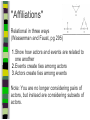
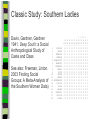
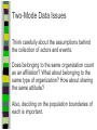
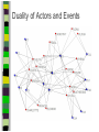
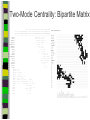
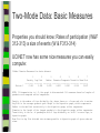
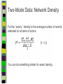
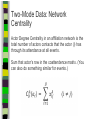
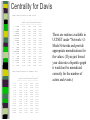
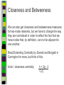
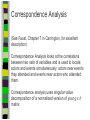
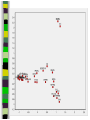
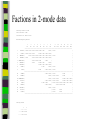
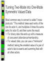
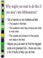
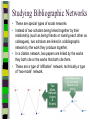
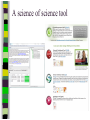
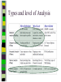
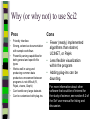
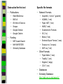
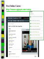
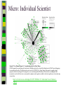
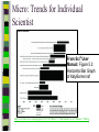
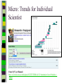
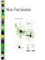
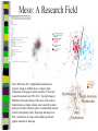
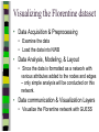
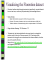
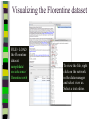
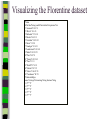
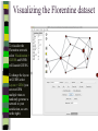
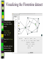
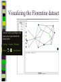
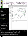
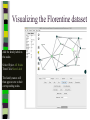
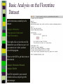
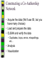
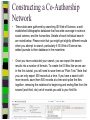
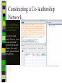
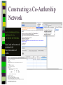
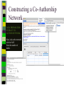
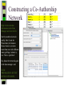
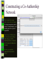
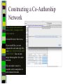
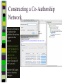
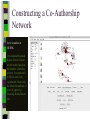
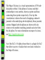
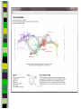
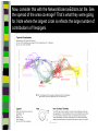
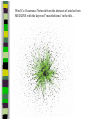
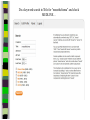
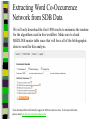
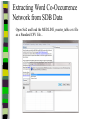
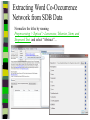
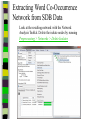
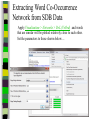
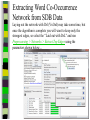
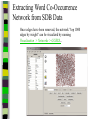
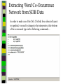
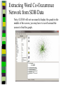
Unit 7: Affiliations Data and
Bibliographic Research
ICPSR
University of Michigan, Ann Arbor
Summer 2015
Instructor: Ann McCranie
"Affiliations"
Relational in three ways
(Wasserman and Faust, pg 295)
1.Show how actors and events are related to
one another
2.Events create ties among actors
3.Actors create ties among events
Note: You are no longer considering pairs of
actors, but instead are considering subsets of
actors.
Classic Study: Southern Ladies
Davis, Gardner, Gardner
1941. Deep South: a Social
Anthropological Study of
Caste and Class
See also: Freeman, Linton.
2003 Finding Social
Groups: A Meta-Analysis of
the Southern Women Data)
1
EVELYN
2
LAURA
3
THERESA
4
BRENDA
5 CHARLOTTE
6
FRANCES
7
ELEANOR
8
PEARL
9
RUTH
10
VERNE
11
MYRNA
12 KATHERINE
13
SYLVIA
14
NORA
15
HELEN
16
DOROTHY
17
OLIVIA
18
FLORA
1
E
1
1
0
1
0
0
0
0
0
0
0
0
0
0
0
0
0
0
2
E
1
1
1
0
0
0
0
0
0
0
0
0
0
0
0
0
0
0
3
E
1
1
1
1
1
1
0
0
0
0
0
0
0
0
0
0
0
0
4
E
1
0
1
1
1
0
0
0
0
0
0
0
0
0
0
0
0
0
5
E
1
1
1
1
1
1
1
0
1
0
0
0
0
0
0
0
0
0
6
E
1
1
1
1
0
1
1
1
0
0
0
0
0
1
0
0
0
0
7
E
0
1
1
1
1
0
1
0
1
1
0
0
1
1
1
0
0
0
8
E
1
1
1
1
0
1
1
1
1
1
1
1
1
0
1
1
0
0
1
9
E
1
0
1
0
0
0
0
1
1
1
1
1
1
1
0
1
1
1
1
0
E
0
0
0
0
0
0
0
0
0
0
1
1
1
1
1
0
0
0
1
1
E
0
0
0
0
0
0
0
0
0
0
0
0
0
1
1
0
1
1
1
2
E
0
0
0
0
0
0
0
0
0
1
1
1
1
1
1
0
0
0
1
3
E
0
0
0
0
0
0
0
0
0
0
0
1
1
1
0
0
0
0
4
E
0
0
0
0
0
0
0
0
0
0
0
1
1
1
0
0
0
0
Two-Mode Data Issues
Think carefully about the assumptions behind
the collection of actors and events.
Does belonging to the same organization count
as an affiliation? What about belonging to the
same type of organization? How about sharing
the same attitude?
Also, deciding on the population boundaries of
each is important.
Duality of Actors and Events
Two-Mode Centrality: Bipartite Matrix
1
EVELYN
2
LAURA
3
THERESA
4
BRENDA
5 CHARLOTTE
6
FRANCES
7
ELEANOR
8
PEARL
9
RUTH
10
VERNE
11
MYRNA
12 KATHERINE
13
SYLVIA
14
NORA
15
HELEN
16
DOROTHY
17
OLIVIA
18
FLORA
19
E1
20
E2
21
E3
22
E4
23
E5
24
E6
25
E7
26
E8
27
E9
28
E1
29
E11
30
E12
31
E13
32
E14
1
1 2 3 4 5 6 7 8 9 0
E L T B C F E P R V
- - - - - - - - - -
1
1
M
-
1
2
K
-
1
3
S
-
1
4
N
-
1
5
H
-
1
6
D
-
1
7
O
-
1
8
F
-
1
9
E
1
1
1
2
0
E
1
1
1
2
1
E
1
1
1
1
1
1
2
2
E
1
2
3
E
1
1
1 1
1 1
1 1
1
1
1
2
4
E
1
1
1
1
1
1
1
1
1
1
1
1
1
1
1
1
1 1
1 1 1
1 1
1 1 1
1 1 1
1 1 1
1 1 1 1
1
1
1 1
1
1 1 1
1
1 1 1
1
1
1 1
1 1 1 1 1 1 1
1 1 1 1 1
1 1
1
1 1 1
1
1 1
1 1
1 1 1
1 1 1
1 1
1 1
1 1 1 1 1 1
1 1 1
1 1 1
2
5
E
-
2
6
E
1
1 1
1 1
1 1
1
1
1 1
1
1 1
1 1
1
1
1 1
1
1 1
1
2
7
E
1
2
8
E
-
2
9
E
-
3
0
E
-
3
1
E
-
3
2
E
-
1
1
1
1
1
1
1
1
1
1
1
1
1
1
1
1 1 1
1
1 1 1
1 1 1 1 1
1 1 1
1
1
Two-Mode Data: Basic Measures
Properties you should know: Rates of participation (W&F
312-313) a size of events (W & F313-314)
UCINET now has some nice measures you can easily
compute:
2-Mode Cohesion Measures for davis dataset.
Matrix 1
1
2
3
4
5
6
7
Density Avg Dist
Radius Diameter Fragmenta Transitiv Norm Dist
--------- --------- --------- --------- --------- --------- --------0.353
2.306
3.000
4.000
0.000
0.619
0.647
NOTE: If fragmentation is > 0, the graph is disconnected. All measures based on lengths of
geodesics are computed within components.
Density is the number of ties divided by n*m, where these no. of rows and cols in matrix.
Avg Dist is the average geodesic path length in the bipartite graph, within components.
Radius is the smallest eccentricity in the bipartite graph, within components.
Diameter is the length of the longest geodesic in the bipartite graph, within components.
Transitivity is the no. of quadruples with 4 legs divided by no. with 3 or more legs, in
bipartite graph.
Norm Dist is Avg Dist divided into minimum possible in bipartite graph of given node-set
sizes.
Two-Mode Data: Network Density
For the “actors,” density is the average number of events
attended by all pairs of actors.
You can do something similar for event density.
Two-Mode Data: Network
Centrality
Actor Degree Centrality in an affiliation network is the
total number of actors contacts that the actor (i) has
through its attendance at all events.
Sum that actor's row in the coattendence matrix. (You
can also do something similar for events.)
Centrality for Davis
2-Mode Centrality Measures for ROWS of davis
1
EVELYN
2
LAURA
3
THERESA
4
BRENDA
5 CHARLOTTE
6
FRANCES
7
ELEANOR
8
PEARL
9
RUTH
10
VERNE
11
MYRNA
12 KATHERINE
13
SYLVIA
14
NORA
15
HELEN
16
DOROTHY
17
OLIVIA
18
FLORA
1
2
3
4
Degree Closeness Betweenne Eigenvect
--------- --------- --------- --------0.571
0.800
0.097
0.335
0.500
0.727
0.051
0.309
0.571
0.800
0.088
0.371
0.500
0.727
0.049
0.313
0.286
0.600
0.011
0.168
0.286
0.667
0.011
0.209
0.286
0.667
0.009
0.228
0.214
0.667
0.007
0.180
0.286
0.706
0.017
0.236
0.286
0.706
0.016
0.218
0.286
0.686
0.016
0.187
0.429
0.727
0.047
0.220
0.500
0.774
0.072
0.277
0.571
0.800
0.113
0.264
0.357
0.727
0.042
0.201
0.143
0.649
0.002
0.131
0.143
0.585
0.005
0.070
0.143
0.585
0.005
0.070
2-Mode Centrality Measures for COLUMNS of davis
1
2
3
4
Degree Closeness Betweenne Eigenvect
--------- --------- --------- --------0.167
0.524
0.002
0.142
0.167
0.524
0.002
0.150
0.333
0.564
0.018
0.253
0.222
0.537
0.008
0.176
0.444
0.595
0.038
0.322
0.444
0.688
0.065
0.328
0.556
0.733
0.130
0.384
1
2
3
4
5
6
7
E1
E2
E3
E4
E5
E6
E7
8
9
E8
E9
0.778
0.667
0.846
0.786
0.244
0.226
0.507
0.379
10 E10
11 E11
0.278
0.222
0.550
0.537
0.011
0.020
0.170
0.090
12 E12
13 E13
14 E14
0.333
0.167
0.167
0.564
0.524
0.524
0.018
0.002
0.002
0.203
0.113
0.113
These are routines available in
UCINET under “Network->2Mode Networks and provide
appropriate normalizations for
the values. (If you just forced
your data into a bipartite graph
it would not be normalized
correctly for the number of
actors and events.)
Closeness and Betweeness
We can also get closeness and betweenness measures
for two-mode networks, but we have to change the way
they are normalized in order to reflect the fact that we
have nodes that, by definition, can not be adjacent to
one another.
Read Extending Centrality by Everett and Borgatti in
Carrington for more, but think of this.
Actor i closeness centrality:
h + 2g - 2
Cc(i)
Correspondence Analysis
(See Faust, Chapter 7 in Carrington, for excellent
description)
Correspondence Analysis looks at the correlations
between two sets of variables and is used to locate
actors and events simultaneously: actors near events
they attended and events near actors who attended
them.
Correspondence analysis uses singular value
decomposition of a normalized version of your g x h
matrix
Factions in 2-mode data
Starting fitness: 0.000
Final fitness: 0.490
Correlation to ideal: 0.490
Blocked Adjacency Matrix
1
EVELYN
2
LAURA
3
THERESA
4
BRENDA
5 CHARLOTTE
6
FRANCES
7
ELEANOR
8
PEARL
9
RUTH
10
VERNE
11
MYRNA
12 KATHERINE
13
SYLVIA
14
NORA
15
HELEN
16
DOROTHY
17
OLIVIA
18
FLORA
1
2
3
4
5
6
7
8
9
10
11
12
13
14
E1
E2
E3
E4
E5
E6
E7
E8
E9
E10
E11
E12
E13
E14
--------------------------------------------------------------------------------------| 1.000 1.000 1.000 1.000 1.000 1.000
1.000 | 1.000
|
| 1.000 1.000 1.000
1.000 1.000 1.000 1.000 |
|
|
1.000 1.000 1.000 1.000 1.000 1.000 1.000 | 1.000
|
| 1.000
1.000 1.000 1.000 1.000 1.000 1.000 |
|
|
1.000 1.000 1.000
1.000
|
|
|
1.000
1.000 1.000
1.000 |
|
|
1.000 1.000 1.000 1.000 |
|
|
1.000
1.000 | 1.000
|
|
1.000
1.000 1.000 | 1.000
|
----------------------------------------------------------------------------------------|
1.000 1.000 | 1.000
1.000
|
|
1.000 | 1.000 1.000
1.000
|
|
1.000 | 1.000 1.000
1.000 1.000 1.000 |
|
1.000 1.000 | 1.000 1.000
1.000 1.000 1.000 |
|
1.000 1.000
| 1.000 1.000 1.000 1.000 1.000 1.000 |
|
1.000 1.000 |
1.000 1.000 1.000
|
|
1.000 | 1.000
|
|
| 1.000
1.000
|
|
| 1.000
1.000
|
----------------------------------------------------------------------------------------
Density matrix
1
1
2
2
----- ----0.625 0.074
0.153 0.537
Turning Two-Mode into One-Mode
Symmetric Valued Data
Most common way to convert is called "crossproducts." This method takes each entry of the
row for actor A, and multiplies it times the same
entry for actor B, and then sums the result.
• For binary data this ends up with a measure
of concurrent attendance/membership.
• For valued data, you can use a "minimums"
method: taking the smallest value of a pair of
actor's ties to events and summing that with
all other actors.
Other places to go…
• Knoke and Yang: Social Network Analysis (2008)
• Faust: Using Correspondence Analysis for Joint Displays of
Affiliation Networks (in Carrington, Scott and Wasserman)
• Roberts, J. M. Correspondence analysis of two-mode
network data. Social Networks, 22:65-72, 2000.
• "Finding Social Groups: A Meta-analysis of the Southern
Women Data" In Ronald Breiger, Kathleen Carley and
Philippa Pattison (eds.) Dynamic Social Network Modeling
and Analysis. Washington, D.C.:The National Academies
Press, 2003.
• Borgatti, S. P. and M. G. Everett. Network analysis of 2mode data. Social Networks, 19(3):243-269, 1997.
Recent extensions to 2-mode data
• Blockmodeling
•
P Doreian, V Batagelj..., Generalized blockmodeling of two-mode network
data Social Networks, 200
• Large two-mode networks
•
Matthieu Latapy, Clemence Magnien, Nathalie Del Vecchio, Basic notions
for the analysis of large two-mode networks, Social Networks, Volume 30,
Issue 1, January 2008, Pages 31-48
• ERGM/p* models
•
P. Wang, K. Sharpe, G. Robins and P. Pattison, Exponential random graph
models for affiliation networks, Social Networks 31 (1) (2009), pp. 12–25
A demonstration and reminder
• Sci2
• There data available for you to
download on the course webpage.
AN INTRODUCTION TO
BIBLIOGRAPHIC NETWORK
ANALYSIS
Scientometrics is an independent and
diverse field
• Literally, measuring and analyzing
science (all kinds).
• Today we’re just in a tiny little corner
of “bibliometric” analysis
• Co-authorship
• Citation
• But this field covers all sorts of ways
of quantifying and evaluating scientific
efforts.
Bibliographic Network Analysis
• Is often focused on citation or authorship patterns
that can be found within fields
• Co-authorship is pretty clear – shared authorship
of an article
• Citation analysis can be thought of differently. Two
common ways:
• “bibliometric coupling, where two citing articles are similar to the
extent they cite the same literature, and co-citation analysis where
cited articles are similar to the extent they are cited by the same
citing articles” Hummon and Doriean Social Networks Volume 11,
Issue 1, March 1989, Pages 39-63
• Citation networks are an interesting case, because at their
most basic they are directed, acyclic data. (A paper cites a
paper that was written earlier, that older paper can never
cite anything published later.)
Bibliographic network analysis
• Can detect subcommunities in research
fields
• Can (and has been) be used to “map
science”
• Can be used to identify prominent actors in
a research field
• Can be used to identify conflict and
consensus in science
• Can be used to trace the development of
ideas
Why might you want to do this if
you aren’t into bibliometrics?
• Get a handle on an intellectual field
• The people in that field
• The academic work they produce and what
is most cited
• The clusters and divisions of the people
and ideas in the field
• Maybe you just want to find the biggest
stars and greatest hits – there are now
a lot of tools to help you do that.
Studying Bibliographic Networks
• These are special types of social networks
• Instead of two scholars being linked together by their
relationship (such as being friends or naming each other as
colleagues), two scholars are linked in a bibliographic
network by the work they produce together.
• In a citation network, two papers are linked by the works
they both cite or the works that both cite them.
• These are a type of “affiliation” network, technically a type
of “two-mode” network.
Two
Mode
Network
Actors
&
Events
Two Mode turned
into One Mode
Network (Just
Actors)
SCI2 TOOL
DEMONSTRATION
Download the tool and documentation:
https://sci2.cns.iu.edu/
A science of science tool
Types and level of Analysis
Why (or why not) to use Sci2
Pros
•
•
•
•
•
•
Friendly interface
Strong, extensive documentation
with sample workflows
Powerful parsing capabilities for
both general and specific file
types
Works well in using and
producing common data
products so movement between
programs is not difficult (R,
Pajek, visone, Gephi)
Can handle very large datasets
Can be customized with plug-ins
Cons
• Fewer (ready) implemented
algorithms than statnet,
UCINET, or Pajek
• Less flexible visualization
within the program
• Adding plug-ins can be
daunting.
For more information about other
software that could be of interest for
the study of science, see section 8.2 of
the Sci2 user manual for listing and
discussion.
Data suited for this tool
Specific file formats
•
•
Publications
•
•
•
•
•
•
•
Refer/BibIX/enw
BibTeX
ISI Web of Science
Scopus
Google Scholar
Google Citation
•
•
•
•
•
•
•
•
•
•
Funding
•
•
•
Network Formats
NSF Award Search
NIH RePORTER
Scholarly Database
•
Other Formats
•
•
•
•
•
•
GraphML (*.xml or *.graphml)
XGMML (*.xml)
Pajek .NET (*.net)
NWB (*.nwb)
Scientometric Formats
ISI (*.isi)
Bibtex (*.bib)
Endnote Export Format (*.enw)
Scopus csv (*.scopus)
NSF csv (*.nsf)
Pajek Matrix (*.mat)
TreeML (*.xml)
Edgelist (*.edge)
CSV (*.csv)
Databases
Scholarly Database:
http://sdb.cns.iu.edu/search/
Free Online Course:
http://ivmooc.appspot.com/course
Micro: Individual Scientist
From Sci2 User Manual: Figure 5.1: Co-authorship network of Katy Börner
GUESS supports the repositioning of selected nodes. Multiple nodes can be selected by holding down the 'Shift' key and dragging a
box around specific nodes. The final network can be saved via 'GUESS: File > Export Image' and opened in a graphic design
program to add a title and legend. The image above was created using Adobe Photoshop. Node clusters were highlighted and
increased in size, the label font size was increased for emphasis, and a legend was added to clarify the significance of node and edge
size and color.
http://sci2.wiki.cns.iu.edu/display/SCI2TUTORIAL/5.1+Individual+Level+Studies++Micro
Micro: Trends for Individual
Scientist
From Sci2 User
Manual: Figure 5.3:
Horizontal Bar Graph
of KatyBorner.nsf
http://sci2.wiki.cns.iu.edu/display/SCI2TUTORIAL/5.1+Individual+Level+Studies+-+Micro
Micro: Trends for Individual
Scientist
From Sci2 User Manual:
http://sci2.wiki.cns.iu.edu/display/SCI2TUTORIAL/5.2+Institution+Level+Studies++Meso
Micro: Four Scientists
Meso: A Research Field
From: McCranie 2013, unpublished dissertation in
progress. Image in middle above is largest single
component of the paper-citation network of “recovery”
research literature from 1991-2012 . Top right image is
Pathfinder Network Scaling of the most cited works in
transformed co-citation network color coded by content
analysis of articles. Bottom right is co-authorship network
coded by disciplinary field. Data prep and analysis in
Sci2, visualization in visone with added legends and
graphic elements in Inkscape.
36
Simple, but important!
The Demonstration
• Basic Features of Sci2
• Citation and co-authorship networks (with
special emphasis on preparing and
cleaning data)
• Topical analysis and visualization
• Available data and ways to pull it into Sci2
• Questions & discussion
THE BASIC
FUNCTIONALITY
The Basics
• Opening Data
• Data
Preparation
• Preprocessing
• Analysis
• Modeling
• Visualization
Visualizing the Florentine dataset
• Data Acquisition & Preprocessing
• Examine the data
• Load the data into NWB
• Data Analysis, Modeling, & Layout
• Since the data is formatted as a network with
various attributes added to the nodes and edges
– only simple analysis will be conducted on this
network.
• Data communication & Visualization Layers
• Visualize the Florentine network with GUESS
Visualizing the Florentine dataset
•
Florentine families related through business ties (specifically, recorded financial
ties such as loans, credits and joint partnerships) and marriage alliances.
•
Node attributes
•
•
•
Wealth: Each family's net wealth in 1427 (in thousands of lira).
Priorates: The number of seats on the civic council held between 1282-1344.
Totalities: Number of business/marriage ties in complete dataset of 116 families.
•
Edge attributes: Marriage T/F & Business T/F
•
“Substantively, the data include families who were locked in a struggle for
political control of the city of Florence around 1430. Two factions were
dominant in this struggle: one revolved around the infamous Medicis, the other
around the powerful Strozzis.”
More info is at http://svitsrv25.epfl.ch/R-doc/library/ergm/html/florentine.html
and Padgett & Ansell 1993 (
http://home.uchicago.edu/~jpadgett/papers/published/robust.pdf)
•
Visualizing the Florentine dataset
FILE> LOAD
the Florentine
dataset:
sampledata/
socialscience/
florentine.nwb
To view the file, right
click on the network
in the data manager
and select view as.
Select a text editor.
Visualizing the Florentine dataset
*Nodes
id*int label*string wealth*int totalities*int priorates*int
1 "Acciaiuoli" 10 2 53
2 "Albizzi" 36 3 65
3 "Barbadori" 55 14 0
4 "Bischeri" 44 9 12
5 "Castellani" 20 18 22
6 "Ginori" 32 9 0
7 "Guadagni" 8 14 21
8 "Lamberteschi" 42 14 0
9 "Medici" 103 54 53
10 "Pazzi" 48 7 0
11 "Peruzzi" 49 32 42
12 "Pucci" 3 1 0
13 "Ridolfi" 27 4 38
14 "Salviati" 10 5 35
15 "Strozzi" 146 29 74
16 "Tornabuoni" 48 7 0
*UndirectedEdges
source*int target*int marriage*string business*string
9 1 "T" "F"
6 2 "T" "F"
7 2 "T" "F"
9 2 "T" "F"
5 3 "T" "T"
Visualizing the Florentine dataset
To visualize the
Florentine network
select Visualization >
GUESS and NWB
will launch GUESS.
To change the layout
in GUESS select
Layout > GEM (you
can run GEM
multiple times to
randomly generate a
network to your
satisfaction, as seen
to the right).
Visualizing the Florentine dataset
Resize the nodes
according to family
wealth.
Resize Linear
>Nodes> Wealth
From: 1 To: 10
Then click Do Resize
Linear
The results will look
similar to what is
shown to the right
Visualizing the Florentine dataset
Colorize nodes according to how
many seats in government the
family holds.
Colorize > Nodes > Priorates
From :
To:
Do Colorize
Visualizing the Florentine dataset
Switch to the Interpreter at
the bottom of the GUESS
window.
Type the following
commands:
for n in g.nodes:
n.strokecolor = n.color
Note: after typing the first
line hit the Tab key and
after the second line hit
Enter and the commands
will be executed.
Learn more about GUESS script options by looking at the sample .py
files in the sampledata folders and by visiting http://
INSNA SCI2 Workshop
48
5/21/2013
graphexploration.cond.org/documentation.html
Visualizing the Florentine dataset
Add the family labels to
the nodes.
Select Object: All Nodes
Then Click Show Label
The family names will
then appear next to their
corresponding nodes.
Basic Analysis on the Florentine
Dataset
Add betweenness centrality to the
dataset.
Analysis>Networks>
Unweighted & Undirected>
Node betweenness
Then right click to view the new file.
Remember you will have to save it if
you want to use it after you have
closed the program.
Now use the NAT to get basic stats on
the network.
Analysis>Networks>Network
Analysis Toolkit.
It will be reported in your console
window and as a output log in the
data manager.
CO-AUTHORSHIP OF A NEW
JOURNAL
Constructing a Co-Authorship
Network
• Acquire the data (We’ll use ISI, but you
have many choices)
• Load and prepare the data
• CLEAN and verify the data
• Duplicates, loops, errors, misspellings,
etc…
• Analysis
• Visualization
Constructing a Co-Authorship
Network
•
These data were gathered by searching ISI Web of Science, a wellestablished bibliographic database that has wide coverage in science,
social science, and the humanities. Details of each individual search
are noted below. Please note that you might get slightly different results
when you attempt to search, particularly if ISI Web of Science has
added journals to their database in the meantime.
•
Once you have conducted your search, you can export the search
results into a number of formats. To create the ISI files like we we use
in this this tutorial, you will need to save them as “Plain Text.” Note that
you can only export 500 records at a time. If you have a search with
more records, save them 500 records at a time and splice the files
together, removing the notations for beginning and ending files from the
second (and third, etc) set of records you add to your first file.
Network Science Journal Editors
•
•
•
•
•
•
•
•
Alessandro Vespignani
Lada Adamic
Nosh Contractor
Stanley Wasserman
Thomas Valente
Garry Robins
Sanjeev Goyal
Ulrik Brandes
Constructing a Co-Authorship
Network
FILE>LOAD>Networ
kScienceEditors.txt (in
your DATA folder)
You will see some
errors! These are items
that are not journal
articles but books and
chapters. You could
restart your search and
exclude them.
Constructing a Co-Authorship
Network
DATA PREPARATION>
EXTRACT COAUTHOR NETWORK.
Now, look at the network
with the NAT.
Note the number of
nodes.
Constructing a Co-Authorship
Network
DATA PREPARATION>
EXTRACT COAUTHOR NETWORK.
Now, look at the network
with the NAT.
Note the number of
nodes.
Constructing a Co-Authorship
Network
Right click on Author
Information in the Data
Manager and view the file.
Sort by number of articles
and by label. Look for
Wasserman, for instance.
Notice that he is in there
more than once with different
name spellings. Adamic is,
too. This is a problem!
So, choose the network again
in the data manager and
DATA
PREPARATION>DETECT
DUPLICATE NODES
Constructing a Co-Authorship
Network
Now examine the merge
table. Look at the two reports.
It’s clearly not perfect, but it’s
a start. In actual analysis, you
would want to be as precise
as possible.
But for now, CNTRL-Click
the Network and the Merge
Table and go to DATA
PREPARATION> UPDATE
NETWORK BY MERGING
NODES
For this, you need the
aggregation function file
shown.
Constructing a Co-Authorship
Network
Take a look at the number of
nodes (NAT). Compare to the
earlier number.
It should be lower than it was.
If you would like, you can
separate the node and edge files
with FILE> SPLIT NODE AND
EDGE FILES. You can later
merge them together for a new
network.
This can make it easier to
examine and to manipulate or
add columns for nodes.
Constructing a Co-Authorship
Network
Now we will remove
all authors that
published fewer than
3 papers in this
dataset.
PREPROCESSING
>NETWORKS>EX
TRACT NODES
ABOVE OR
BELOW VALUE.
(Enter 2 instead of
the 3 you see.)
Run the NAT again
and see what has
changed.
Constructing a Co-Authorship
Network
Let’s visualize in
GUESS.
I recommend Kamada
Kawai. Resize Linear
for the nodes based on
the number of articles
written. I recommend 1
to 50 for scale, but
experiment. Show only
the labels for authors of
over 10 papers by
choosing Nodes Based
On.
USING A MAP OF SCIENCE
TO “LOCATE” RESEARCH
The Map of Science is a visual representation of 554 subdisciplines within 13 disciplines of science and their
relationships to one another, shown as points and lines
connecting those points respectively. Over top this
visualization is drawn the result of mapping a dataset's
journals to the underlying sub-discipline(s) those journals
contain. Mapped sub-disciplines are shown with size
relative to the number matching journals and color from
the discipline. For more information on maps of science,
see http://mapofscience.com
As of the Sci2 v1.0 alpha release there is a plugin for Sci2
that allows users to visualize their own data overlaid on
the Map of Science.
Load the FourNetSciResearchers.isi file in the ISI flat
format…
To visualize dataset overlaid on the Map of Science run
Visualization > Topical > Map of Science via Journals
The journals titles are
used to determine which
records fit into what subdiscipline. You can view
the journal titles found
and those not found from
the data manager of Sci2.
A single journal can
belong to more than one
sub-discipline and thus so
can the record associated
with that journal. So the
circle sizes are
proportional to the number
of fractionally assigned
records.
Now, consider this with the NetworkScienceEditors.txt file. See
the spread of the area coverage? That’s what they were going
for. Note where the largest circle is reflects the large number of
contributions of Vespigani.
USING THE SCHOLARLY
DATABASE ON A TOPIC
AREA
Word Co-Occurrence Network from the abstracts of articles from
MEDLINE with the keyword “mesothelioma” in the title…
If you have registered for the Scholarly Database then go to
http://sdb.cns.iu.edu and login…
If you do not have an account type in [email protected] and nwb for
the password
Do a keyword search in Title for “mesothelioma” and check
MEDLINE…
Extracting Word Co-Occurrence
Network from SDB Data
We will only download the first 1000 results to minimize the runtime
for the algorithms used in this workflow. Make sure to check
MEDLINE master table since that will have all of the bibliographic
data we need for this analysis.
Your download limit will initially capped at 2000 records at a time. To increase this limit,
please email [email protected]
Extracting Word Co-Occurrence
Network from SDB Data
Save the file somewhere on your computer for
use later in this tutorial… (in this case, if you
can’t sign on to SDB, then you will find a copy
in the DATA folder.)
Extracting Word Co-Occurrence
Network from SDB Data
• The topic similarity of basic and aggregate units of science
can be calculated via an analysis of the co-occurrence of
words in associated texts. Units that share more words in
common are assumed to have higher topical overlap and
are connected via linkages and/or placed in closer
proximity.
• Extract Word Co-Occurrence Network creates a weighted
network where each node is a word and edges connect
words to each other, where the strength of an edge
represents how often two words occur in the same body of
text together.
• This algorithm is a shortcut for extracting a directed
network using Extract Directed Network, and then
performing bibliographic coupling using
Extract Reference Co-Occurrence (Bibliographic Coupling)
Network.
Extracting Word Co-Occurrence
Network from SDB Data
Open Sci2 and load the MEDLINE_master_table.csv file
as a Standard CSV file…
Extracting Word Co-Occurrence
Network from SDB Data
Normalize the titles by running
Preprocessing > Topical > Lowercase, Tokenize, Stem, and
Stopword Text and select “Abstract”…
Extracting Word Co-Occurrence
Network from SDB Data
Run Extract Word Co-Occurrence Network and set the
parameters as shown below…
Extracting Word Co-Occurrence
Network from SDB Data
To see more information about your network run
Analysis > Networks > Network Analysis Toolkit…
Extracting Word Co-Occurrence
Network from SDB Data
Look at the resulting network with the Network
Analysis Toolkit. Delete the isolate nodes by running
Preprocessing > Networks > Delete Isolates
Extracting Word Co-Occurrence
Network from SDB Data
Apply Visualization > Networks > DrL (VxOrd) and words
that are similar will be plotted relatively close to each other.
Set the parameters to those shown below…
Extracting Word Co-Occurrence
Network from SDB Data
Laying out the network with Drl (VxOrd) may take some time, but
once the algorithm is complete you will want to keep only the
strongest edges, so select the “Laid out with DrL” and run
Preprocessing > Networks > Extract Top Edges using the
parameters shown below…
Extracting Word Co-Occurrence
Network from SDB Data
Once edges have been removed, the network "top 1000
edges by weight" can be visualized by running
Visualization > Networks > GUESS…
Extracting Word Co-Occurrence
Network from SDB Data
In order to make use of the DrL (VxOrd) force directed layout
we applied, we need to change to the interpreter at the bottom
of the screen and type in the following commands…
Extracting Word Co-Occurrence
Network from SDB Data
Note, GUESS will not necessarily display the graph in the
middle of the screen, you may have to scroll around the
screen to find the graph.
Just the beginning – check the Sci2 website for
more!