Download Atomic Force Microscopy:

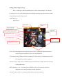
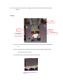
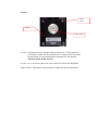
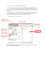
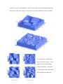
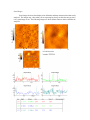
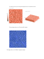
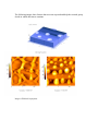
Atomic Force Microscopy:
A Guide to Understanding and Using
the AFM
Galloway Group
Spring 2004
Atomic Force Microscopy
I)
II)
How it works and why we do it?
Theory and History
i) STM vs. AFM
ii) Scanning Probe Microscopy
iii) Theory
(1) Repulsive and Attractive Forces
iv) Characterization at microscopic level
(1) Image of sample at this scale
(2) Different modes of imaging will reveal different properties of the sample
(3) What does Analysis tell us?
(a) RMS Roughness
(b) Distances, changes in heights
III)
IV)
V)
Getting Started Step by Step
Hardware
i) AFM components
(1) Scanner, Scan head, tips,
Software
i) Imaging Software
(1) Scan Head Control Screen
(2) Image screen
(a) Scan Size
(b) Scan Speed
(c) Set P
(d) Gain
ii) Image Analysis Software
VI)
Getting ready to scan
i) Sample Preparation and Handling
ii) Logging in Sample
iii) AFM tip check
VII)
How to take an Image
i) Contact Mode
ii) Non-Contact Mode
VIII)
How to Analyze an image
i) Flatten
(1) What it means
ii) Analysis
(1) Region
(2) Line
iii) Presentation
(1) 3D, 2D. Multi
IX)
Good image vs. Bad image
(1) Noise
(2) Out of Range
(3) Bad Sample
(4) Changing Scanning parameters
X)
Previous Problems and Tips
Note to Reader
The purpose of this paper is to provide the new user of the Atomic Force Microscope (AFM) with
a more concise version of the manual in order to start utilizing the AFM. I will go into a little bit
of the theory of why it works but this is mainly something to get you started. It is always
necessary to continue your knowledge of this machine and try to explore using different aspects
of the software.
Introduction
The Atomic Force Microscope is an instrument that can analyze and characterize samples
at the microscope level. This means we can look at surface characteristics with very accurate
resolution ranging from 100 µm to less than 1µm.
The AFM operates by allowing an extremely fine sharp tip to either come in contact or in very
close proximity to the sample that is being imaged. This tip is usually a couple of microns long
and often less than 100Å in diameter. The tip is located at the free end of a cantilever that is 100
to 200µm long. The sample is then scanned beneath the tip. Different Forces either attract or
repeal the tip. These deflections are recorded and processed using imaging software; the resulting
image is a topographical representation of the sample that was just imaged. If you want to know
about the sample rather than just a view of its surface, there are different imaging modes that are
used for different types of analysis. Either different hardware or scanning techniques are required
to obtain the data necessary for the analysis. The AFM can measure a number of characteristic
properties of the sample that other forms of microscopy cannot reproduce.
Brief History and Comparison
In 1986, the Atomic Force Microscope was invented by Gerd Binning to overcome a
limitation of the AFM’s predecessor, the Scanning Tunneling Microscope. The STM could only
image materials that could conduct a tunneling current. The AFM opened the door to imaging
other materials, such as polymers and biological samples that do not conduct a current. In some
cases, the resolution of STM is better than AFM because of the exponential dependence of the
tunneling current on distance. The force-distance dependence in AFM is much more complex
when characteristics such as tip shape and contact force are considered. The AFM wins in terms
of versatility easily. In comparison, with other forms of microscopy the AFM is better or
comparable.
•
AFM versus SEM:
Compared with Scanning Electron Microscope, AFM provides extraordinary topographic
contrast direct height measurements and unobstructed views of surface features (no
coating is necessary).
•
AFM versus TEM:
Compared with Transmission Electron Microscopes, three-dimensional AFM images are
obtained without expensive sample preparation and yield far more complete information
than the two-dimensional profiles available from cross-sectioned samples.
•
4. AFM versus Optical Microscope:
Compared with Optical Interferometric Microscope (optical profiles), the AFM provides
unambiguous measurement of step heights, independent of reflectivity differences
between materials.
Interactive Forces
The main difference between these types of microscopy and the AFM is, as the name
suggests, interactive forces between the sample and the tip. The force most commonly associated
with atomic force microscopy is an interatomic force called the van der Waals force. The
relation between this force and distance is shown in Fig. 1.
In the contact region, the cantilever is
held less than a few angstroms (10-10m) from
the sample surface, and the interatomic force
between the cantilever and the sample is
repulsive. In the non-contact region, the
cantilever is held on the order of tens to
hundreds of angstroms from the sample surface,
and the interatomic force between the cantilever
Figure 1: van de Waals force vs. distance
and sample is attractive. Different
scanning modes operate in different regions of this curve: Non–contact in the attractive region,
contact mode in the repulsive and intermittent or tapping mode fluctuates between the two.
It is easier to understand this curve if you think of the point of the tip like a group of
atoms interacting with the surface which essentially another group of atoms.
At the right side of the curve, the atoms are separated by a large distance. As the atoms
are gradually brought together, they first weakly attract each other. This attraction increases until
the atoms are so close together that their electron clouds begin to repel each other
electrostatically. This electrostatic repulsion progressively weakens the attractive force as the
distance continues to decrease. Following the graph, the force goes to zero when the distance
reaches a couple of angstroms. Anything closer than this, the total van der Waals force becomes
positive (repulsive). This distance will not change, therefore any more attempt to force the
sample and tip closer will result in deformation or damage to the sample or the tip.
There are two other forces that arise during the scan: a capillary force that is caused by a
build-up of water, which is normally present without an inert environment, on the tip; the force
caused by the cantilever itself, which is like a force caused by a compressed spring.
Characterization at the microscopic level
Even though, the process of the scanning is straightforward and can be done at times
with your total attention, not all images are accurate representations of the actual topography of
the sample. There are parameters that can
be changed in each scan and other forces
outside the interatomic forces that can
alter the image or the sample. For
QuickTime™ and a TIFF (Uncompressed) decompressor are needed to see this picture.
example, Fig. 2 is a 5-micron scan of
Copper that has been treated with
Tetrahydrofuran. The two lines of raised
peaks are not actual features on the
Figure 2: 5 micron Cu scan containing two lines of noise
sample but points during the scan when the sample was inadvertently disturbed. A discussion of
what is a good image versus a bad one is located at the end of this paper.
ProScan Image Processing software provided with the AFM is used to process and
analyze the image, which can make it easier to recognize an image that is a misrepresentation.
Processing allows for modification of the image in order to remove artifacts without modifying
the surface features. In Analysis, quantitative measurements can be taken of individual cross
sections or surface regions. Surface statistics such as distance measurements, peak-to-valley
measurements and surface roughness are a few commonly acquired measurements.
Getting Started Step-by-Step
Now we will begin a discussion of the process of how to take an image. We will start
by giving an overview of the components of the AFM, the options on the probe head move mode
screen and options on the image screen.
AFM components
Probe Head
Probe Head
Laser On/Off
switch
Laser intensity and
position indicators
Position Sensitive Photo detector
Laser beam
steering screws
PSPD adjustment screws
XY Translation Stage
XY Translation
Screws
Cartridge Position Screws
Probe Head: Interchangeable head slips into place on the XY translation; different heads have
certain scan mode capabilities, houses laser and photodiode
XY Translation Stage: Holds probe head, movable in XY direction by XY translation screws and
in Z direction by controls in software
Position Sensitive Photo detector (PSPD): Detects laser deflections, which is then converted into
a topographical map
PSPD adjustment screws: controls position of PSPD; screw on left controls up and down
adjustment; screw on right controls left right adjustment
Laser Beam Steering Screws: controls position of laser on back of cantilever
Laser Intensity and Position Indicators: Lights represent laser position and intensity on photo
detector
Cartridge
Cartridge
Tip
Cassette
Cassette Holder
Tip Holder
Cartridge: removable part of probe head that holds the cassette which in turn holds the
tip.
Cassette: removable from cartridge and is held in position be holder and three balls
which fit into slots in cassette
Tip: actually cantilever chip, which contains the probe tips
View from optical microscope of
cantilevers
Scanner
Scanner
Screws
Scanner
Sample Holder
Scanner: component that moves sample under tip during scan. Voltage applied to
piezoelectric scanner tube housed inside moves sample precise increments
back and forth. Size at bottom indicates maximum size scan possible.
Extremely fragile handle with care
Scanner screws: unscrewing these four screws allows for removal and installation
Sample Holder: holds sample and piezoelectric scanner tube directly underneath
Proscan Data Acquisition and Image Processing Software
Once again, this is just an overview of the essentials that are needed for basic AFM
operation. After basic knowledge and familiarity with the instrument has been gained then a
more in depth understanding and knowledge of different capabilities can be acquired by reading
the manuals.
Proscan Data Acquisition controls the AFM and collects the data then converts it to an image. It
operates primarily in two modes: Move Mode and Image Mode. Each screen has certain
controls for the imaging processes but contain some of the same displays.
Data Acquisition Screen in Move Mode
Shortcut Icons
Status Bar
Active Display
Up/Down Control
of Stage
Image Gallery
Auto approach
Height of stage
When opening the Proscan Data Acquisition software, the opening screen is the move mode
screen. The stage can be controlled
Oscilloscope
Image Analysis
Now we will discuss the difference between a good image vs. a bad one. When I say good image
I do not only mean image quality but being able to recognize features which are really present
and some which are artifacts of the scan.
Bad Images
Bad images likes those which have poor resolution or which contain unreadable features
are not preferrable but can still tell us something about our sample. For instance, say the group
is producing sample which contain some sort of chemical on the surface. If the images show
lots of particles on the surface or irregular formations, then it can be assumed that the process
being used to manufacture these samples is not viable. These images are two examples of
manufacturing problems detected by the AFM. The image on the left shows coagulations of
what is supposed to be a thin film on the surface. The right hand image shows how dirt on the
sample ruins the scan as well, in this case it is not known wither the dirt came from the
manufacturing process or the imaging process.
With bad images, a lot of parameters can affect the quality of suitable sample images.
These changes will result in bad images that would have been fine if not for these changes in
parameters. One such example is deformation or dullness of tip. The AFM assumes that the tip
used for every scan is sharp and intact. These next two images are scan of Tungsten taken with
a tip that was either worn down by use or may have been broken during the change of samples.
To the left are the 2-deminsional
images of the same sample. At first
glance there is no sign that these
scans are bad images. It was only
seen through the 3-D representation
and questioning the truth of the
scan. A new operator will probably not be able to pinpoint these bad images. Unfamiliarity with
how different materials look does not allow it, but with experience it should be possible.
Other parameters that could be changed
that affect the scan are the options in the Pro
Scan Data Acquisition Image Mode Screen. The
options like Set Point and Scan Speed can not
only affect the image but can harm the sample.
The gain however only will affect the image.
Changing the set point effects the force that is
the tip senses between it and the sample. If the
Set Pont is too low then the scan will
not scan because the force is not
strong enough between the sample
and the tip to cause deflections of the
cantilever. If the Set Point is too high
then the tip can actually deform the
sample or itself. Unless it’s a really
hard material the sample will deform.
The images to the right shows the
deformation of the sample by a high Set Point.
There are other outside factors that cause bad images that at times cannot be controlled.
Ambient noise both acoustic and electric can affect the scan . Noise can be pinpointed as reason
for bad images when the rest of the scan is fine but there are random placed peaks or lines of
peaks on one scan but not he other.
The image above shows how the entire image how noise can affect the end of a graph.
This could have been caused by a constant noise that lasted a couple of seconds.
QuickTime™ and a TIFF (Uncompressed) decompressor are needed to see this picture.
The image above shows lines of noise that are very unlike the rest of the scan. These
were caused by sharp noises rather than a long standing noise.
Good Images
Good images are those that display clear definition and sharp characteristics that can be
analyzed. The images may show what you are expecting but it may not this does not govern if
it is a good image or not. The following images are show definite features which could then be
analyzed.
The following scans represent images that displayed what we wanted them to show.
The two images above are of Teravicta RF Switches.
The images above is of a Diblock Copolymer sample.
The following images show features that were not expected and help the research group
decide in which direction to continue.
Images of Diblock Copolymers.