Download UWB RTLS for Construction Equipment Localization

UWB RTLS for Construction Equipment Localization:
Experimental Performance Analysis and Fusion with Video Data
Hassaan Siddiqui
A Thesis
in
Concordia Institute for
Information Systems Engineering
Presented in Partial Fulfillment of the Requirements
for the Degree of Master of Applied Science (Quality Systems Engineering)
at
Concordia University
Montreal, Quebec, Canada
September 2014
© Hassaan Siddiqui
CONCORDIA UNIVERSITY
School of Graduate Studies
This is to certify that the thesis prepared
By:
Hassaan Siddiqui
Entitled:
UWB
RTLS
for
Construction
Equipment
Localization:
Experimental
Performance Analysis and Fusion with Video Data
and submitted in partial fulfillment of the requirement for the degree of
Master of Applied Science (Quality Systems Engineering)
complies with the regulations of the University and meets with the accepted standards with
respect to originality and quality.
Signed by the final examining committee:
Dr. M. Mannan
Chair
Dr. N. Bouguila
CIISE Examiner
Dr. A. Bagchi
External Examiner (BCEE)
Dr. Amin Hammad
Supervisor
Approved by
Chair of Department or Graduate Program Director
m
Dean of Faculty
ABSTRACT
UWB RTLS for Construction Equipment Localization: Experimental Performance
Analysis and Fusion with Video Data
Hassaan Siddiqui
Construction sites are well known for their dynamic and challenging nature. Several researchers
are investigating the application of various Real-time Location Systems (RTLSs) for improving
the safety and productivity of construction projects. When integrated with real-time data analysis
systems, RTLS can contribute to make the construction environment smarter and safer by
identifying safety hazards and inefficient resource configurations. Previous research shows that
the Ultra-Wideband (UWB) technology, an emerging type of RTLS, is suitable for the
identification and tracking of construction resources. However, a thorough study to evaluate the
impact of the factors that affect the performance of the UWB RTLS in construction projects is
still required. This research investigates the performance of UWB RTLSs in indoor and outdoor
environments along with the evaluation of the factors which affect their performance. Moreover,
the harsh environment of construction sites and the complex nature of construction projects
provide numerous challenges for an individual technology to deliver accurate information in a
timely manner. Therefore, this research also proposes a Multi-Sensor Data Fusion (MSDF)
approach which leverages the benefits of video recording and image processing as a
complimentary data source. It was found that the UWB RTLS is an effective tool to monitor
construction resources; however, some of the UWB data can be missing or erroneous and the
quality of the data can be improved by applying a suitable data enhancement method to
accurately localize construction equipment. Furthermore, it was noted that the MSDF approach
has the potential to better localize construction equipment by overcoming the limitations of
UWB RTLS.
iii
ACNOWLEDGEMENT
First and foremost, I would like to express my sincere gratitude to my supervisor, Dr. Amin
Hammad for his intellectual support, encouragement and patience. His advice and criticism was
my most valuable asset during my studies. The joy and enthusiasm he has for his research was
contagious and motivational for me, even during tough times of this pursuit.
Besides my supervisor, I would like to thank Mr. Faridaddin Vahdatikhaki for his valued
assistance in performing the tests and processing the test data. I am also very thankful to Mr.
Mohammad Soltani for his appreciated support in the implementation of image processing. I
would also like to thank Mr. Pierre Vilgrain from PCL Constructors Westcoast Inc. for his
support in the realization of the outdoor test.
In addition, the support from all of the research group members was very invaluable. My sincere
thanks also go to Ms. Mahsa Rafiee, Mr. Shayan Setayeshgar and Mr. Ali Motamedi for their
help in various aspects of this research.
I dedicate this thesis to my wife, my parents and my brothers for their endless encouragement
which is the essence of this accomplishment.
iv
TABLE OF CONTENTS
List of Figures ............................................................................................................................... vii
List of Tables ................................................................................................................................. xi
List of Abbreviations ................................................................................................................... xiii
CHAPTER 1
INTRODUCTION ................................................................................................. 1
1.1
General Review ................................................................................................................ 1
1.2
Research Objectives ......................................................................................................... 2
1.3
Thesis Organization.......................................................................................................... 2
CHAPTER 2
ITERATURE REVIEW ........................................................................................ 4
2.1
Introduction ...................................................................................................................... 4
2.2
Ultra-Wideband Real-Time Location System .................................................................. 4
2.3
Applications of UWB RTLS in Construction Management ............................................ 7
2.4
Data Enhancement Methods........................................................................................... 18
2.4.1
Simplified Correction Method ................................................................................ 19
2.4.2
Optimization-based Method.................................................................................... 20
2.5
Data Fusion .................................................................................................................... 22
2.6
Multi-Sensor Data Fusion .............................................................................................. 24
2.6.1
2.7
Techniques used for Multi-Sensor Data Fusion...................................................... 26
Applications of Multi-Sensor Data Fusion..................................................................... 29
2.7.1
Applications in Construction Management ............................................................ 29
2.7.2
Other MSDF Positioning Applications ................................................................... 31
2.8
Summary ........................................................................................................................ 32
CHAPTER 3
3.1
EXPERIMENTAL PERFORMANCE ANALYSIS OF UWB RTLS ................ 33
Introduction .................................................................................................................... 33
v
3.2
Factors affecting the UWB System’s Performance........................................................ 33
3.3
Experimental Work ........................................................................................................ 37
3.3.1
Indoor Dynamic Tests ............................................................................................. 38
3.3.2
Outdoor Dynamic Tests .......................................................................................... 55
3.4
Summary, Conclusions and Recommendations ............................................................. 87
CHAPTER 4
FUSING UWB AND VIDEO DATA FOR CONSTRUCTION EQUIPMENT
LOCALIZATION ......................................................................................................................... 89
4.1
Introduction .................................................................................................................... 89
4.2
Comparison of UWB and Video Technologies for Construction Projects .................... 89
4.3
Proposed Approach ........................................................................................................ 91
4.3.1
Hardware Components............................................................................................ 91
4.3.2
Software Components ............................................................................................. 92
4.4
Implementation and Case Study..................................................................................... 96
4.4.1
Design of Experiment ............................................................................................. 96
4.4.2
Implementation ....................................................................................................... 98
4.4.3
Analysis................................................................................................................. 109
4.5
Summary and Conclusions ........................................................................................... 117
CHAPTER 5
CONCLUSIONS AND FUTURE WORK ....................................................... 119
5.1
Summary of Research .................................................................................................. 119
5.2
Research Contributions and Conclusions..................................................................... 120
5.3
Limitations and Future Work ....................................................................................... 121
REFERENCES ........................................................................................................................... 122
APPENDIX A – UWB System Configuration User Manual...................................................... 127
APPENDIX B – Detection and Localization MATLAB Code for Image Processing ............... 143
vi
APPENDIX C – Data Fusion MATLAB Code .......................................................................... 144
APPENDIX D – List of Related Publications ............................................................................ 146
vii
LIST OF FIGURES
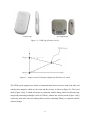
Figure 2.1 – UWB Tags (Ubisense, 2013a) .................................................................................... 6
Figure 2.2 – Angle of Arrival Technique (adapted from Ghavami et al., 2004) ............................ 6
Figure 2.3 – Time Difference of Arrival Technique (adapted from Ghavami et al., 2004) ........... 7
Figure 2.4 – Schematic Diagram of UWB Systems (adapted from Zhang et al., 2012b)............... 7
Figure 2.5 – Relationship between Offset, Precision, and Accuracy (Maalek & Sadeghpour,
2013) ............................................................................................................................................... 9
Figure 2.6 – Comparison of Cumulative Accuracy Curves for AOA vs. TDOA & AOA (Maalek
& Sadeghpour, 2013) .................................................................................................................... 10
Figure 2.7 – UWB sensors positions A1 to A6 (Saidi et al., 2011) .............................................. 11
Figure 2.8 – UWB tags mounted at different heights (nominally 1 m, 2 m, and 3 m) (Saidi et al.,
2011) ............................................................................................................................................. 12
Figure 2.9 – UWB Tracking in Lay Down Yard (Saidi et al., 2011)............................................ 13
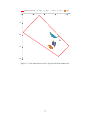
Figure 2.10 – Area Layout for Static Test in Fully-Furnished Office (Cho et al., 2010) ............. 15
Figure 2.11 – Results of Open Space Dynamic Tests (Cho et al., 2010)...................................... 16
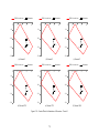
Figure 2.12 – Predetermined Five Paths for Closed Space Dynamic Test (Cho et al., 2010) ...... 17
Figure 2.13 – Illustration of Correction Process (Vahdatikhaki & Hammad, 2014) .................... 20
Figure 2.14 – Flowchart of Iterative Correction Process (Vahdatikhaki & Hammad, 2014) ....... 21
Figure 2.15 – Flowchart of Optimization-based Method (Vahdatikhaki et al., 2014).................. 22
Figure 2.16 – The development model (Opitz et al., 2004) .......................................................... 24
Figure 2.17 – High Level Architecture of Multi-Sensor Data Fusion System ............................. 26
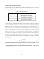
Figure 3.1 – Test Settings ............................................................................................................. 39
Figure 3.2 - Area Settings ............................................................................................................. 40
Figure 3.3 - Tag's Performance Comparison for P1 ..................................................................... 42
vii
Figure 3.4 - Tag's Performance Comparison for P2 ..................................................................... 42
Figure 3.5 - Tag's Performance Comparison for P3 ..................................................................... 43
Figure 3.6 - Tag's Performance Comparison for P4 ..................................................................... 43
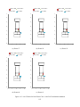
Figure 3.7 – Area Settings for Indoor Dynamic Tests – I............................................................. 45
Figure 3.8 – Design of Experiment for Indoor Dynamic Tests - I................................................ 46
Figure 3.9: Performance Comparison of Wired UWB System and Wireless UWB System ........ 48
Figure 3.10 – Investigation of Impact of Dilution of Precision Phenomenon .............................. 50
Figure 3.11 - Area Settings for Indoor Dynamic Tests - II........................................................... 51
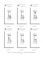
Figure 3.12 - Wired and Wireless UWB System – II – Raw Data ............................................... 53
Figure 3.13 – Wired and Wireless UWB System – II – Averaged Data ...................................... 54
Figure 3.14 – Wired and Wireless UWB System – II – Slope – Raw Data.................................. 55
Figure 3.15 – UWB Settings for Outdoor Test ............................................................................. 56
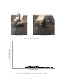
Figure 3.16 – Compact tags with magnet for Construction Equipment ....................................... 57
Figure 3.17 – Tag positions on excavator ..................................................................................... 57
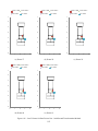
Figure 3.18 – Area Settings for Outdoor Dynamic Test ............................................................... 60
Figure 3.19 – Tracked Roller for Outdoor Dynamic Test ............................................................ 60
Figure 3.20 – Control Charts for Update Rate Analysis ............................................................... 64
Figure 3.21 – Cumulative Probability vs. Update Rate Analysis for Outdoor Dynamic Test ...... 65
Figure 3.22 – Raw Data of All Tags for Period 1 ......................................................................... 66
Figure 3.23 – All Tags Averaged with Δt = 3 sec ........................................................................ 67
Figure 3.24 – Geometric Constraints for Outdoor Dynamic Test ................................................ 67
Figure 3.25 – Results of Simplified Correction Method (All Tags Averaged for Δt = 3 sec) ...... 68
Figure 3.26 – Results of Simplified Correction Method (S3 & S4 Average for Δt = 1 sec) ........ 68
Figure 3.27 - Results of Optimization based Method (All Tags Averaged for Δt = 3 sec) .......... 69
viii
Figure 3.28 – Site View on May 22, 2014 before Visit ................................................................ 70
Figure 3.29 – UWB Sensor Panel ................................................................................................. 72
Figure 3.30 – UWB Covered Area for Full Scale Outdoor Test .................................................. 73
Figure 3.31 – Site Conditions for Each Day ................................................................................. 75
Figure 3.32 – Excavator Tags’ Positions for Full Scale Outdoor Test (Excavator image is taken
from Google, 2014) ....................................................................................................................... 76
Figure 3.33 – Raw Data Analysis of Five Tags for Full Scale Outdoor Test ............................... 77
Figure 3.34 – Excavator Position at 12:53 PM on Day 4 ............................................................. 78
Figure 3.35 – Schematic View of Orientation of Excavator (Excavator image is taken from
Google, 2014) ............................................................................................................................... 78
Figure 3.36 – Scatter Plots for Orientation of Excavator – Period 1 ............................................ 79
Figure 3.37 – Angle Calculation for Accuracy Assessment (Excavator image is taken from
Google, 2014) ............................................................................................................................... 80
Figure 3.38 – Actual Angle (θa) Calculation for Accuracy Assessment ...................................... 81
Figure 3.39 – Error Distribution for Accuracy Assessment – Period 1 ........................................ 81
Figure 3.40 – Tracked Movement of Excavator for Period 2 ....................................................... 83
Figure 3.41 – Schematic View of Orientation of Excavator (Excavator image is taken from
Google, 2014) ............................................................................................................................... 84
Figure 3.42 – Scatter Plots for Orientation of Excavator – Period 2 ............................................ 85
Figure 3.43 – Excavator Position .................................................................................................. 86
Figure 3.44 – Error Distribution for Accuracy Assessment – Period 2 ........................................ 86
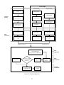
Figure 4.1 – Proposed Approach Overview .................................................................................. 91
Figure 4.2 –Proposed Approach ................................................................................................... 93
Figure 4.3 – Visual IDs for Equipment Identification .................................................................. 95
Figure 4.4 – Association Error Explanation ................................................................................. 96
ix
Figure 4.5 – Design of Experiment for MSDF Case Study .......................................................... 97
Figure 4.6 – Detection Results .................................................................................................... 100
Figure 4.7 – Pixels Conversion ................................................................................................... 103
Figure 4.8 – Measurement of Attributes of Field of View (adapted from MATLAB (2014a)) . 104
Figure 4.9 – Coordinate Transformation Using First Method .................................................... 105
Figure 4.10 – Control Points ....................................................................................................... 106
Figure 4.11 – Coordinate Transformation using Second Method............................................... 107
Figure 4.12 – First 6 Frames for Data Fusion Case 1 with First Transformation Method ......... 111
Figure 4.13– Last 5 Frames for Data Fusion Case 1 with First Transformation Method ........... 112
Figure 4.14 – Incorrect Association during Fusion Process with First Transformation Method 113
Figure 4.15 – First 6 Frames for Data Fusion Case 1 with Second Transformation Method ..... 114
Figure 4.16 – Last 5 Frames for Data Fusion Case 1 with Second Transformation Method ..... 115
Figure 4.17 – Correct Association during Fusion Process with Second Transformation Method
..................................................................................................................................................... 116
x
LIST OF TABLES
Table 2.1 – Fusion Stages & Techniques (Smith & Singh, 2006; Hall, 1992) ............................. 28
Table 3.1 – Factors affecting UWB System ................................................................................. 36
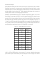
Table 3.2 – Effect of Number of Sensors on the UWB System (adapted from Zhang, 2010) ..... 37
Table 3.3 – Overview of Experimental Work ............................................................................... 37
Table 3.4 - Tag IDs ....................................................................................................................... 38
Table 3.5 – Update Rate and Missing Data Rate Analysis ........................................................... 41
Table 3.6 – Description of Indoor Dynamic Tests – I .................................................................. 44
Table 3.7 – AUR and MDR Analysis for Indoor Dynamic Tests - I ............................................ 46
Table 3.8 – OC and GCs for Indoor Dynamic Tests - I ................................................................ 47
Table 3.9 – Accuracy Analysis for Tests 1A and 2A ................................................................... 49
Table 3.10 – AUR and MDR Analysis for Indoor Dynamic Tests - II ......................................... 52
Table 3.11 – AUR and MDR Analysis for Slope Test ................................................................. 54
Table 3.12 – Results of Indoor Wireless Connectivity Test ......................................................... 58
Table 3.13 – Results of Outdoor Wireless Connectivity Test ...................................................... 59
Table 3.14 – AUR Analysis for Outdoor Dynamic Test .............................................................. 61
Table 3.15 – MDR Analysis (msec) for Outdoor Dynamic Test .................................................. 61
Table 3.16 – MDR Analysis (sec) for Outdoor Dynamic Test ..................................................... 62
Table 3.17 – AUR & MDR Analysis for Period 1 ........................................................................ 74
Table 3.18 – Mean & Standard Deviation Analysis for Period 1 ................................................. 74
Table 3.19 – AUR & MDR Analysis for Period 2 ........................................................................ 82
Table 4.1 – Comparison of UWB & Image Processing Technologies for Construction Projects 90
Table 4.2 – AUR & MDR Analysis for MSDF Case Study ......................................................... 98
Table 4.3 – Description of Detector Outcomes .......................................................................... 101
xi
Table 4.4 – Analysis of Detector Outcomes ............................................................................... 101
Table 4.5 – Performance Metrics for Detector ........................................................................... 102
Table 4.6 – Values of Attributes of Field of View ..................................................................... 104
Table 4.7 – Coordinates of Control Points.................................................................................. 106
Table 4.8 – Data Association Cases ............................................................................................ 108
Table 4.9 – Data Fusion Cases Occurrence ................................................................................ 109
Table 4.10 – Data Association Results ....................................................................................... 110
xii
LIST OF ABBREVIATIONS
2D
Two Dimensional
3D
Three Dimensional
AoA
Angle of Arrival
API
Application Programming Interface
AUR
Actual Update Rate
BIM
Building Information Modeling
CAD
Computer-Aided Design
DoE
Design of Experiment
DoP
Dilution of Precision
ENCS
Easting and Northing Coordinate System
EoI
Equipment of Interest
EUR
Expected Update Rate
FM
Fusion Module
FoV
Field of View
fps
Frames per second
GC
Geometric Constraint
GCS
Global Coordinate System
GPS
Global Positioning System
GUI
Graphical User Interface
IEC
International Electrotechnical Commission
IF
Information Filter
IP
Internet Protocol
IPC
Image Processing Component
xiii
ISO
International Standards Organization
k-NN
k - Nearest Neighbors
LAN
Local Area Network
LCS
Local Coordinate System
LoS
Line-of-Sight
MDR
Missing Data Rate
MRM
Minimum Reset Measurements
MSDF
Multi-Sensor Data Fusion
OC
Operational Constraint
PTZ
Pan-Tilt-Zoom
RC
Remote Controlled
RF
Radio Frequency
RFID
Radio Frequency Identification
RTLS
Real-Time Location System
SCS
Smart Construction Site
SIF
Static Information Filtering
TDoA
Time Difference of Arrival
TL
Tolerance Limit
UCS
Ultra-Wideband Coordinate System
UM
Ultra-Wideband Module
UWB
Ultra-Wideband
VCS
Video Coordinate System
VM
Video Module
WLAN
Wireless Local Area Network
xiv
CHAPTER 1
INTRODUCTION
1.1 General Review
Real-time information is the essence of smart decision making. In construction operations, realtime information about the equipment and workers can certainly assist in reinforcing the safety
and improving the overall efficiency. The availability of real-time information is also the basis
for the concept of Smart Construction Site (SCS) which aims at improving the overall safety,
sustainability and efficiency of a construction project by making the real-time information about
the project available to all the stakeholders in order to enable them to make right decisions at the
right time. Zhang et al. (2009) describes SCS as an intelligent integrated setup where: (1) the
information about the entire environment is acquired from the sensors attached to moving
objects; (2) equipment’s path is automatically planned; and (3) every stakeholder, including the
staff-members, has intelligent assistance from various agents providing information and
decision-making strategies. The advancements in Real-time Location Systems (RTLSs), such as
Radio Frequency Identification (RFID) and Global Positioning System (GPS), have enabled
researchers to investigate the applicability of these systems to automate the on-site data
collection process.
Ultra-Wideband (UWB) technology, a type of RTLS, has been investigated by several
researchers for the identification, localization and tracking of construction resources. The UWB
technology has the potential to track and visualize construction resources on site and increase the
awareness level of the construction staff in near real time. UWB RTLS provides several
advantages over other RTLS including long and reliable range, accurate real-time positioning
and capability to handle the multipath issue (Rodriguez, 2010). However, a thorough
investigation of the performance of the UWB system under uncertain conditions of a
construction site is still required. Therefore, this research is intended to realize the challenges of
the construction projects and investigate the applicability of the UWB system for construction
projects under dynamic conditions.
Furthermore, the distinct nature of each construction project and the challenges they offer, the
uncertain and highly dynamic conditions of a construction site, and the diversity of the
construction equipment impose enormous challenges. Therefore, depending on a single
1
technology or system to deliver the required accurate information in a timely manner becomes
unreliable. Some research has been done to utilize multiple independent technologies under a
Multi-Sensor Data Fusion (MSDF) framework to cope with the challenges of the construction
environment. MSDF technique is recognized for overcoming the limitations of the individual
sensing technologies by combining the sensory data from multiple sources (Rafiee et al., 2013;
Elmenreich, 2002; Luo et al., 2002). Therefore, this research also intends to overcome the
limitations of the UWB RTLS by using image processing data as a complimentary sensory
source.
1.2 Research Objectives
The objectives of this research are to:
(1). Evaluate the impact of the factors affecting the performance of wired and wireless
UWB systems in construction projects through indoor and outdoor testing.
(2). Investigate the possibility of improving the construction equipment UWB tracking by
leveraging the data from video processing.
1.3 Thesis Organization
This research is presented as follows:
Chapter 2 Literature Review: this chapter reviews the literature about the UWB RTLS and
MSDF technologies along with their applications in construction management. Furthermore, two
data enhancement methods are also reviewed which are useful for improving the accuracy of the
data from the UWB RTLS.
Chapter 3 Experimental Performance Analysis of UWB RTLS: this chapter evaluates the factors
that affect the performance of the UWB system and analyzes the performance of the wired and
the wireless UWB systems for indoor and outdoor construction environments under dynamic
conditions through several experiments.
2
Chapter 4 Fusing UWB and Video Data for Construction Equipment Localization: in this chapter
an MSDF based approach is proposed for the localization of the construction equipment by
fusing data from two sensory data sources, which are the UWB RTLS and camera. The
implementation of the proposed approach is also presented in this chapter along with the its
validation through a case study.
Chapter 5 Conclusions and Future Work: this chapter summarizes the present work, highlights
the contributions and concludes the findings. This chapter also includes the recommendations for
the usage of the UWB RTLS on real construction sites and highlights the future research
directions.
3
CHAPTER 2
ITERATURE REVIEW
2.1 Introduction
In this chapter the previous research on UWB RTLS and Multi-Sensor Data Fusion (MSDF)
technologies are reviewed. Also, the applications of these technologies in construction
management are discussed. This literature review is aimed to investigate the capabilities and
applicability of the UWB RTLS and the MSDF techniques for improving the safety and
productivity of construction projects.
This chapter is organized as follows: Section 2.2 reviews the UWB RTLS technology; Section
2.3 reviews the applications of UWB RTLS in construction management; Section 2.4 reviews the
data enhancement techniques for enhancing UWB data; Section 2.5 reviews data fusion models;
Section 2.6 examines and compares the MSDF techniques; Section 2.7 highlights the
applications of MSDF in construction management; and Section 2.8 summarizes the reviewed
literature.
2.2 Ultra-Wideband Real-Time Location System
RTLS provides the information, in real time, about the location of assets. Malik (2009) describes
RTLS as a system which enables users to manage and analyze the information regarding where
assets or people are located. Malik further explains that an RTLS consists of the following parts:
(1) tags, which are attached to the assets; (2) sensors, which reads the tags’ data; (3) location
engine, which is a software used to localize the tags; (4) middleware, which connects the
location engine data with a software application; and (5) end-user software application.
UWB is a special type of RTLS which transmits and receives short duration pulse of Radio
Frequency (RF) energy (Lee et al. 2009). Malik (2009) explains that UWB is a carrier-less radio
technology that uses wide bandwidth (i.e. exceeding 500 MHz or 20 percent of the arithmetic
center frequency, whichever is lower), and is normally used in short-range wireless applications.
Malik (2009) also explained that UWB-based positioning has several advantages over other
RTLS technologies, which includes: high accuracy, better performance in challenging RF
environments, no interference from other RF systems, and relative immunity to multipath fading.
4
The immunity to multipath fading is because UWB pulses are narrow and occupy the entire
UWB bandwidth. The early applications of UWB technology were primarily related to radar.
The UWB system used in this research is developed by Ubisense Group PLC (Ubisense, 2013a).
This UWB system comprises of the following parts: (1) tags, for monitoring assets; (2) sensors,
for reading tags; (3) timing cables or wireless bridges, for the connectivity of sensors with each
other and with the host computer; (4) location engine, for calculating tag’s position using various
techniques; and (5) software application for recording data. The tags come in various form
factors (Figure 2.1) depending on the asset to be monitored e.g. for tracking people, slim tag
(Figure 2.1(a)) is used whereas for tracking equipment, compact tag (Figure 2.1(b)) is used. The
sensors are installed at the boundaries of the monitored area which forms a cell; and the higher
the number of sensors in a cell, the better the accuracy of the tag’s position estimated by the
UWB system. Each sensor gathers two types of information from the signal received from the
tag: the angle of the signal, and the time when the signal is received (Maalek & Sadeghpour,
2013). The UWB system utilizes two positioning techniques to estimate the tag’s position
depending on the information received by the sensors, which are Angle of Arrival (AOA) and
Time Difference of Arrival (TDOA). In the AOA technique, the angle of the arrived signal is
measured at several sensors by routing the main lobe of a directional antenna or an adaptive
antenna array. Each measurement forms a radial line from the sensor to the tag. For 2D
localization, the location of the tag is defined at the intersection of two directional lines of
bearing, as shown in Figure 2.2 (Ghavami et al., 2004). In the TDOA technique, the difference in
the arrived signal’s time at two different sensors is calculated. Then, each time difference is
converted to a hyperboloid with a constant distance difference between the two sensors, where
the location of the tag is the intersection of the two corresponding hyperboloids, as shown in
Figure 2.3 (Ghavami et al., 2004). AOA has advantage over the TDOA as it does not require
synchronization of the sensors nor an accurate timing reference (Ghavami et al., 2004); however,
TDOA requires more cabling for accurate timing reference.
5
(a) Slim Tags
(b) Compact tags
Figure 2.1 – UWB Tags (Ubisense, 2013a)
Figure 2.2 – Angle of Arrival Technique (adapted from Ghavami et al., 2004)
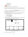
The UWB system supports two modes of communication between sensors with each other and
with the host computer, which are: the wired and the wireless, as shown in Figure 2.4. The wired
mode (Figure 2.4(a)), in which all sensors are connected with the timing cables, localizes the tags
using both positioning techniques (AOA & TDOA); whereas the wireless mode (Figure 2.4(b))
works only with AOA, since the timing cables (used for estimating TDOA) are replaced with the
wireless bridges.
6
Figure 2.3 – Time Difference of Arrival Technique (adapted from Ghavami et al., 2004)
(a) Wired System
(b) Wireless System
Figure 2.4 – Schematic Diagram of UWB Systems (adapted from Zhang et al., 2012b)
2.3 Applications of UWB RTLS in Construction Management
Although UWB RTLS has several industrial applications, the focus of this section is to highlight
the applications of UWB RTLS in construction management. As not much literature is available
in this domain, therefore some related literature is reviewed in detail.
7
Maalek & Sadeghpour (2013) evaluated the performance of UWB RTLS under certain
conditions, which occur very often on a real construction site. They conducted seven different
experiments to assess the accuracy of location estimated by the UWB RTLS. For each
experiment, they simulated various construction site scenarios which are related to: (1) the
presence of metallic items within the monitored area, (2) UWB signal blockage, (3) metallic
items tracking, (4) wireless mode of UWB system, (5) tracking multiple items, and (6) the effect
of number of UWB sensors (total of 8 sensors).
To measure the accuracy of data, Maalek & Sadeghpour (2013) used the Distance Root Mean
Squared (DRMS) (Equation (2.1)) method for 2D accuracy whereas Mean Radial Spherical Error
(MRSE) (Equation (2.2)) method was used for 3D accuracy. These methods are different from
the average of Euclidean distances between the actual location and the estimated location, as
they provide a single value to represent the accuracy and also take into account the probability
distribution.
∑
∑
√
∑
(2.1)
∑
√
∑
(2.2)
Along with the 2D and 3D accuracies, Maalek & Sadeghpour (2013) also calculated the
precision of data (Equations (2.3) & (2.4)), which is the standard deviation; and the offset
(Equations (2.5) & (2.6)), which is the distance between the average estimated locations and the
actual location. The relationship between offset, precision and accuracy is demonstrated in
Figure 2.5.
√
∑
√
∑
∑
√
(2.3)
∑
∑
(2.4)
√
(2.5)
√
(2.6)
8
Maalek & Sadeghpour (2013) also found that the phenomenon called Dilution of Precision
(Langley, 1999; Mahfouz et al., 2008), which is related to the geometry of the cell, also has a
strong impact on the accuracy of the UWB system.
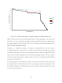
Furthermore, by removing the timing cables and comparing the accuracy of the UWB system
with and without the timing cables, Maalek & Sadeghpour (2013) found that the overall accuracy
using only AOA measurements is less than 53 cm in 2D (Figure 2.6(a)) and less than 63 cm in
3D (Figure 2.6(b)). They also noted that the relative error shows an average decrease of 114.2%
in 2D accuracy and 58.09% in 3D; however, despite this decrease, the average accuracy using
only AOA measurement is still less than 1 m, with 27 cm of accuracy in 2D and 37 cm in 3D.
Through this analysis, they concluded that removing the timing cables will decrease the
accuracy, but the UWB system can still provide a location accuracy of less than one meter.
To simulate the signal blockage scenario, Maalek & Sadeghpour (2013) turned off the sensor
with best Line of sight (LoS). In this case, the location would be estimated without the best
signal. However, this will not simulate the exact signal blockage scenario because multipath
effects would not be considered, which are present in the real signal blockage situation. Also,
this simulation would represent a special case of another experiment which they conducted by
reducing the number of sensors. So this experiment, with a turned off sensor, can be considered
as an experiment with seven sensors.
(a) Offset approaches zero
(b) Precision approaches zero
(c) Legend
Figure 2.5 – Relationship between Offset, Precision, and Accuracy (Maalek & Sadeghpour, 2013)
9
(a) 2D
(b) 3D
Figure 2.6 – Comparison of Cumulative Accuracy Curves for AOA vs. TDOA & AOA (Maalek &
Sadeghpour, 2013)
As all the variables for these experiments were simulated in an indoor environment and all
tracked items were in a static mode, the nature of real construction site, which is mostly outdoor
and highly dynamic, can affect the UWB system’s performance significantly.
Saidi et al. (2011) also conducted several experiments to evaluate the static and dynamic
performance of a UWB RTLS. Their focus was to design the testing of this type of RTLS for
personnel applications in open-space and in realistic construction conditions. Moreover, they
also developed a mathematical static model for estimating position errors of this system. Saidi et
al. (2011) also identified twenty three factors that influence the accuracy of the UWB system,
which include the calibration error, hardware (antenna type, receiver orientation) and the tags'
roll, pitch, and yaw angles. They also suggested that the effect of the orientation (yaw angle) of
the UWB tag is one of the most important factors.
They designed the open-space experiments to evaluate, firstly, the 3D errors and, secondly, the
sensitivity of the 3D errors to inaccuracies in the measured positions of the sensors. Within this
set of experiments, two experiments were conducted; the first one with the sensor locations
known to be within ±1 mm and the second one with the sensor locations known to be within ±20
cm. For the former experiment, they used an industrial total station to measure the locations of
sensors whereas for the latter one, they used a differential GPS with a measurement error of 20
cm to 30 cm. They positioned six UWB sensors (see Figure 2.7), where line-of-sight (LOS) to all
sensors was available throughout the coverage area, and mounted three UWB tags, spaced at 1
meter intervals with the highest tag at 3m (see Figure 2.8), on a fiberglass pole. Then, they
established a ground truth model and placed multiple benchmarks within the open-space field.
10
Figure 2.7 – UWB sensors positions A1 to A6 (Saidi et al., 2011)
To collect the data, they moved the UWB tag pole from one benchmark to the next. At each
benchmark, the data were collected for one minute and the UWB tag pole was placed at 48
benchmarks. This procedure was repeated twice, first the calibration items, which are the
locations of the UWB sensors and reference tag, were measured with the total station whereas for
the second time, the calibration items were measured with differential GPS receiver. It took them
almost 10 hours to setup and collect data for each of the above experiments.
Saidi et al. (2011) also highlighted that the case in which the locations of the calibration items
were measured with the total station, i.e. with the accuracy of ±1 mm, represented the ideal setup
procedure for the system which might not be achievable in the field due to practical
considerations.
Saidi et al. (2011) defined the 2D and 3D measurement errors as the Euclidean distance between
the coordinates estimated by the UWB system and measured with the total station. They found
that the average 2D and 3D errors were 0.087 m ± 0.010 m and 0.466 m ± 0.040 m, respectively,
where the averages of the standard error of the mean are represented by + or – intervals. As the
3D error is significantly larger than the 2D error, they suggested that several sensors must be
mounted at different heights, at either equal or close to equal distance to each other, to minimize
the 3D error. In addition, they also noted that the 3D error decreases as tag elevation increases.
However, they found no correlation between tag elevation and the 2D error. Also, they noted that
the mean error decreases with the decrease in elevation whereas the standard deviation remains
relatively constant at the three elevations. Furthermore, they noted that the error is low at the
center of the coverage area, which was expected based upon the manufacturer’s specifications.
11
Figure 2.8 – UWB tags mounted at different heights (nominally 1 m, 2 m, and 3 m) (Saidi et al., 2011)
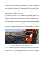
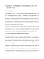
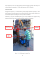
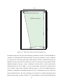
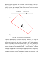
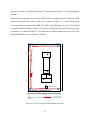
Saidi et al. (2011) conducted the second set of experiments in a lay down yard (see Figure 2.9),
which was for steel components of a power plant, to evaluate the dynamic performance of the
system under realistic construction conditions. They selected an active work zone of about
100,000 m2 within the lay down yard, positioned the UWB sensors at the boundary of the yard,
and tagged several construction workers and machines with UWB tags. They did not consider
the height (z-coordinate), of the tracked item/person in this set of experiments. They
synchronized the timestamps of UWB system with a construction robotic total station (RTS)
within 1s and registered both location measurement systems, i.e. UWB and RTS, to a common
coordinate system. They mounted a UWB tag, with a 1 Hz update rate, and a mini RTS prism on
a construction worker's helmet and collected data, without interruption, for 32 min and 14 s or
1287 position points with both systems where they used the RTS measurements as ground truth.
They calculated the location errors by calculating the difference between the UWB and RTS
measurements and found that almost 47% of all errors were less than 1.25 m whereas 87% were
within 2.5 m. They defined an unusual activity if, at an UWB update rate of 1 Hz, the difference
12
between one location reading and the next is greater than 2.5 m, as the worker might be jumping
or falling. They also proposed that if this type of unusual activity happens, the data might be fed
to any alert system. They also proposed the optimization of UWB covered area as it will reduce
the installation cost along with impacting the tracked resources. Furthermore, from this
experiment, they also noted that at a distance of greater than 100 m, the UWB signals were out of
range whereas the RTS was able to track the workers.
The system used by Saidi et al. (2011) was a UWB only based on TDOA and did not use AOA.
Furthermore, out of the two sets of experiments conducted by Saidi et al. (2011), one set was
conducted in an open-space field whereas the other set was conducted in a construction lay down
yard. The real construction environment normally include both indoor and outdoor conditions,
however this research only focuses on the outdoor conditions of the construction environement
because the indoor conditions are more challenging in terms of establishing a ground truth
measurement, due to the obstacles and the limitations in the power output of the UWB system
used. They also assumed the conditions to be ideal if they have minimal obstacles and reflections
and have a good medium for RF signal propagation.
Figure 2.9 – UWB Tracking in Lay Down Yard (Saidi et al., 2011)
Cho et al. (2010) analysed the reliability of the wireless UWB system’s data for tracking assets
in indoor construction sites. They conducted static and dynamic tests in various building spaces.
They also developed an error model, to minimize the positioning errors of wireless UWB system,
using some statistical techniques including regression analysis, outlier detection, and Kalman
13
filtering. While conducting these indoor tests, they kept at least one receiver in direct LoS from
any location of the monitored area.
The static tests were conducted in four different types of indoor building spaces; open space,
wood-framed building site, steel-framed building site and fully-furnished office area. For
assessing the accuracy of the wireless UWB system, they used the difference in the Euclidean
distance between the tag’s known position and the UWB estimated position. For the open space
test, they elevated the tag by 35 cm to give it a better LoS and obtained an accuracy of 17.02 cm.
For the wood-framed building site, they obtained an accuracy of 46 cm with the tag elevated by
94 cm whereas when the tag was on the floor, they obtained an accuracy of 63 cm. They also
collected the data, with the same test layout, where a human was carrying the tag with an
elevation of 130 cm. For this data, the accuracy of the wireless UWB system was 59 cm. In this
case, they expected to obtain better accuracy as the tag was more elevated but the accuracy
dropped down. Therefore, they concluded that the human body has negative affect on the quality
of communication between a tag and the sensors. They also found that this conclusion is aligned
with the literature (Welch et al., 2002). For the steel-framed building site, when the tag was on
the floor, they obtained an accuracy of 56 cm whereas when the tag was elevated by 104 cm,
better accuracy was obtained i.e. 38.6 cm. From the results of the wood-framed site and the steelframed site tests, they concluded that accuracy seems to be more sensitive to location and facing
angle of sensors as there is no significant accuracy difference between the wood-framed site and
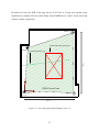
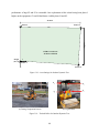
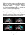
the steel-framed site. For the static test in fully-furnished office area (Figure 2.10), they obtained
an average accuracy of about 41 cm at the floor level whereas when the tag was elevated by 104
cm, they obtained an accuracy of 50 cm. In this test layout, the tag was also carried by a human
which significantly affected the accuracy based on human’s orientation.
Moreover, Cho et al. (2010) conducted dynamic error tests in open space and closed space
indoor construction sites. The primary objective of the dynamic error test was to provide a
framework to minimize the positioning errors of the UWB data in a specific area in real time.
They compared the differences between the tag’s positions estimated by the UWB system and
the probable known positions. As in the dynamic tests, they expected more random errors as the
tag was carried by a human moving with various speeds and orientations; therefore to improve
the accuracy of the estimated positions in real time, they applied the Kalman filter algorithm.
They also used Kalman smoother algorithm for smoothing the data. Furthermore, they detected
14
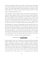
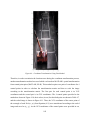
multiple outliers using the Rosner's test (Rosner, 1975; Rosner, 1983). For the open space test,
they moved the tag in a pre-determined S-shape path. The tag’s location was updated every 50
ms. They corrected the UWB data using the Kalman filter and the Kalman smoother and
analyzed the estimated path. This corrected path is shown in Figure 2.11(a) and by analyzing the
corrected path, they observed that the data was distributed over a wider range due to extreme
noisy data points which they call outliers. In this test, they identified 13 points (0.3% of the total
points) as outliers using the Rosner's algorithm and then removed the 13 outliers. They observed
that although removing the outliers slightly improves the paths created by the Kalman filter and
Kalman smoother, the outliers between paths were not detected by the algorithm. Through this
analysis, they concluded that the outlier algorithm should be independently applied to each path
with its own Rosner's test values rather than all the paths as a whole.
Figure 2.10 – Area Layout for Static Test in Fully-Furnished Office (Cho et al., 2010)
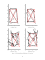
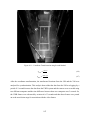
For the closed space dynamic test, Cho et al. (2010) used five pre-determined straight paths (see
Figure 2.12) and the tag, which was elevated by 104 cm, was carried by a human along all the
pre-determined paths at a normal walking speed. The location of the tag was updated every
10ms. They collected data sets for four cycles and estimated and removed the outliers
15
individually by each path and each cycle. They found that each path, in a different cycle, showed
a different rate of outlier detection and, on average, about 9% of the points were detected as
outliers for each cycle. Through this analysis, they concluded that the outlier algorithm works
better when applied to an individual path.
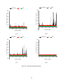
(a) Raw Data Analysis with Kalman Filter
(b) Outliers Removed
Figure 2.11 – Results of Open Space Dynamic Tests (Cho et al., 2010)
To further improve the wireless UWB system’s positioning accuracy, Cho et al. (2010) proposed
an error modelling process. This error model was based on the closed space dynamic test, where
the five straight paths were determined. During developing the error model, they used single
regression analysis to find a best fitting line from the scattered data. They separately analysed the
x and y values of the collected data. Firstly, they compared the differences between the observed
positions and the estimated positions. Then, they calculated the accuracy based on the distance
between the two positions. To estimate regression equations, for each line segment (each line
segment corresponds to each straight path) they considered several possible linear and non-linear
regression lines. In this process, they selected a line equation only if it improved the overall
positioning accuracy in conjunction with the line equation of the other axis. They also considered
several non-linear equations but no equation actually improved the positioning accuracy.
Furthermore, out of five line segments, the developed regression lines for three line segments
were unable to improve the accuracy. In this situation, they assumed that the heavy metallic
items (bookshelf and mailboxes) standing against the walls near this space may have distorted
the UWB signals. To overcome this issue, they further divided this straight line into three
16
sections: hallway entrance, hallway, and end of hallway. Then they applied the regression
equation only to the middle section of that line, and after removing the outliers, the raw data was
applied to the other two sections. With the revised error model, the accuracy of that line
improved significantly.
Figure 2.12 – Predetermined Five Paths for Closed Space Dynamic Test (Cho et al., 2010)
In order to validate the proposed error model, Cho et al. (2010) collected a new set of data and
analysed with the pre-determined outlier constraints and regression equations for the five predetermined paths. They found that, using the proposed error modelling process, the positional
accuracy improved by about 27.8%. They also suggested that the Kalman filter and the Kalman
smoother perform better with the proposed error modelling process. Furthermore, they
recommended that the developed error modelling processes can be extended to other wireless
tracking technologies to improve their accuracy as well.
Cho et al. (2010) concluded that the accuracy of the UWB system is low in dynamic and closed
space situation than in static and open space situation. Furthermore, through this study, they
validated that although the accuracy of the wireless UWB system is lower than the wired one, the
wireless UWB system is still capable of tracking mobile assets in indoor construction sites with
17
an accuracy of about 50 cm in static condition and 65 cm in dynamic condition for a highly
congested closed space. The wireless UWB system was used in this research, however this
analysis does not take into account the conditions of outdoor construction environment as the
tests were conducted in indoor environments.
Zhang et al. (2012a) proposed a post-processing method to improve data quality and transform
the location data into useful information that can be used for near real-time decision support
systems. Moreover, they tested the UWB system using the proposed method to estimate the pose
of a crane and concluded that the pose of the crane boom can be estimated in near real time using
the UWB system. Although they performed a thorough analysis using the UWB system, they
only used the wired UWB system.
Vahdatikhaki & Hammad (2014) proposed a framework based upon the integration of UWB
RTLS with a simulation model of construction operations in order to enhance the simulation
model continuously by capturing motion information about the truck and excavator. Their
proposed framework provides a method for capturing, processing, analysing, filtering and
visualizing the equipment states along with enhancing the accuracy of the equipment stateidentification. The data processing is done by considering the equipment-specific geometric and
operational constraints. Although their proposed framework is tracking-technology-independent
and can work with various types of RTLS technologies, they used wired UWB system in an
indoor environment to demonstrate the feasibility of their proposed framework.
Rodriguez (2010) investigated the utilization of UWB system in improving productivity and
safety of construction projects by collecting data from a construction site and organizing them
into useful information needed for management. They found that UWB is an effective tool to
monitor construction resources because it provides accurate information in real time.
2.4 Data Enhancement Methods
Two data enhancement methods are reviewed which are used for enhancing the data from the
UWB system. These methods are: (1) Simplified Correction Method (SCM), and (2)
Optimization-based Method (OM). Both of these methods are based on Operational Constraints
(OCs) and Geometric Constraints (GCs), where OCs limits the tags’ movement, e.g. moving too
18
fast, and GCs relates different tags with respect to the geometric consistency of the equipment,
e.g. fixed distance.
2.4.1 Simplified Correction Method
Vahdatikhaki & Hammad (2014) proposed a method to reduce the measurement errors in which
sensory data is captured from the construction site and processed by the data processor. This
method focuses on adjusting the data according to the GCs and OCs, in which it is iteratively
validated that a set of GCs and OCs are satisfied for each data point. The assumption of this
method is that several UWB tags are installed on different parts of different pieces of the
equipment and each tag has a unique ID.
Vahdatikhaki & Hammad (2014) described that this method is implemented using the following
steps: (1) The UWB tags are grouped according to their geometric relationships with respect to
the equipment to which they are attached; (2) each tag’s data are averaged over a short period of
time (Δt); (3) if there are any missing data, it will be calculated using interpolation; (4) the data
are corrected based upon the operational constraints and the geometric constraints; and (5)
several tag’s data are averaged.
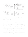
Vahdatikhaki & Hammad (2014) further explained these steps as (see Figure 2.13): in step 2,
averaging over time refers to averaging a tag’s location over several points in time; in step 3,
new data is created for the missing data points using interpolation; in step 4, data correction
refers to the adjustment of the tags' data, iteratively, to ensure that a set of OCs and GCs are
satisfied at every given point in time. The OC is applied so that the difference between two
consecutive tag data entries does not violate the maximum operational speed limit of the
equipment; whereas, the GC is applied based upon a fixed geometric relation between any given
two tags attached to a rigid body; and, in step 5, the data can be further enhanced by representing
several tags by an intermediate point by averaging several tags’ data which are attached to the
same rigid body. The flowchart for this iterative process is shown in Figure 2.14.
19
(a) Averaging of several readings over Δt
(b) Corrections based on the OCs
(c) Corrections based on the GCs
(d) Averaging of several tags’ data
Figure 2.13 – Illustration of Correction Process (Vahdatikhaki & Hammad, 2014)
2.4.2 Optimization-based Method
Vahdatikhaki et al. (2014) proposed a correction method which is committed to determining the
minimum amount of correction applicable to each tag that will result in a pose of construction
equipment with a minimum amount of violation from all GCs and OCs. The assumption of this
method is that the equipment is equipped with a set of UWB tags and that every rigid part of the
equipment is represented by at least two tags. Furthermore, for the compensation of the missing
or erroneous data, this method performs a multi-step processing on the raw data gathered from
the tags before they can be used for the pose analysis.
Vahdatikhaki et al. (2014) explained that the process, which consists of several steps to increase
the accuracy of the pose estimation (Figure 2.15), begins with the averaging of data over a period
of time and applying interpolation for filling the missing data. Then the optimization-based
correction is applied, which has further two phases: (1) identification of center of rotation, and
(2) identification of the required corrections. The first phase of the correction ensures that the
series of captured data respect the relationship with the center of rotation; whereas the second
20
phase minimizes the tag’s data errors in such a wat that a number of GCs and OCs of the
equipment are respected. Finally, once the errors are corrected, the pose of the equipment is
identified using the corrected data.
Figure 2.14 – Flowchart of Iterative Correction Process (Vahdatikhaki & Hammad, 2014)
21
Figure 2.15 – Flowchart of Optimization-based Method (Vahdatikhaki et al., 2014)
2.5 Data Fusion
Integration of data from multiple sources resulting in reliable and feature-rich information is
Nature’s approach. Creatures interpret signals from multiple sensors to judge the surrounding
environment. For example, the human brain interprets signals from the five body senses (sight,
sound, smell, taste, and touch) with knowledge of the environment to create and update a
dynamic model of the world, which allows humans to interact with the environment and make
decisions about present and future actions (Elmenreich, 2002).
Data fusion, a multidisciplinary field, is the process of integrating data or information in order to
estimate the state of a system or an entity. This integration enhances the confidence, improves
reliability, and reduces ambiguity of measurements for estimating the state of entities in
engineering systems. It also enhances the completeness of fused data that is required for
22
estimating the state of engineering systems (Shahandashti et al., 2011). Data fusion has three
general goals: increasing the (1) completeness, (2) conciseness, and (3) correctness.
Completeness measures the amount of data, conciseness measures the uniqueness of object
representations in the integrated data, and correctness measures the correctness of data, i.e.,
whether the data conform to the real world or not (Dong & Naumann, 2009).
Data Fusion is applied in various modern systems like air traffic control, surveillance systems,
defense systems, etc. These systems are commonly developed in accordance with different
industrial and governmental standards. Data fusion requires dealing with simultaneous
engineering processes i.e., one has to work with multiple developers simultaneously on the
embedded software items, resource management and the hardware items, e.g. sensors and
effectors, over extended time (Opitz et al., 2004). Although this integration process can be
managed by the application of formal methods, these methods have some limitations too. Formal
methods are generally at the abstract level, but systems and data integration mostly requires indepth knowledge of the systems under consideration.
Various formal methods and international standards have been developed to integrate data from
various systems and sources. Opitz et al. (2004) investigated that how the software development
standards can be tailored for specific data fusion processes and highlights some of the widely
used international standards. Opitz et al. (2004) further explains that ISO/IEC 12207 is one of the
commonly accepted international standards, which was prepared by a joint technical committee
of the International Organization for Standardization (ISO) and the International Electrotechnical
Commission (IEC) (IEEE/EIA, 1998). Some other standards include: AQAP-160 standard which
is used in NATO projects and is a modification of the ISO/IEC 12207 standard; and the DoDSTD-2167A is widely used for military projects (DoD, 1988).
According to ISO/IEC 12207, the development process is divided into the following steps
(Opitz, et al., 2004; IEEE/EIA, 1998): 1) System requirements analysis and design; 2) Software
requirements analysis,; 3) Software architectural design; 4) Software detailed design; 5) Software
coding and testing; 6) Software integration and qualification testing; and 7) System integration
and qualification testing. Opitz et al. (2004) developed a simplified development model, as
shown in Figure 2.16, based on the standard and suggested that at each step, traceability of
23
requirements, consistency, test coverage, appropriateness, conformance, and feasibility should be
ensured.
Figure 2.16 – The development model (Opitz et al., 2004)
2.6 Multi-Sensor Data Fusion
Multi-Sensor Data Fusion (MSDF), also known as Sensor fusion, refers to the integration of
sensory data from multiple sensors to provide more reliable and accurate information. This
fusion of information reduces overall uncertainty and offers potential advantages including, but
24
not limited to, redundancy, correctness, reliability and thus increases the accuracy with which the
environment is observed by the system.
Multiple sensors increase reliability of the system by providing redundant and timely information
about the environment. This redundant information from multiple sensors allows efficient
environment perception that is hard to achieve using single sensor. Multiple sensors also provide
more timely information as a result of either the actual speed of operation of each sensor, or the
parallel processing that may be achieved as part of the integration process. Also in this scenario,
even when a sensor is deprived, the system is still capable of compensating lacking information
by reusing data obtained from other sensors (Luo et al., 2002).
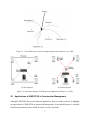
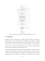
Figure 2.17 shows a high level architecture of MSDF. It can be observed that sensors perceive
the environment through the transfer of Energy, Material Wealth, Mass, and Information
(EMMI) (Langford, 2012). Then, through EMMI, sensors transfer data to the fusion process,
which then converts the data into meaningful information which is then available to the decision
makers.
MSDF is a rapidly evolving research area and requires multidisciplinary knowledge in systems
control, systems integration, signal processing, artificial intelligence, probability, statistics, and
specific application area (Luo et al., 2002). In recent years, prospective research has been
conducted to explore the applicability of various techniques for multi-sensor data fusion systems
and its applications. Gustafsson et al. (2002) explored potential applications of sequential Monte
Carlo methods in positioning, navigation, and tracking problems. Smith & Singh (2006)
reviewed various approaches for target tracking. Massimiliano et al. (2011) applied sensor fusion
for people tracking and Nazar (2009) compared two statistical estimation and noise filtering
techniques, based upon Kalman Filtering, for multi-sensor data fusion.
25
Environment
EMMI
Sensor A
EMMI
EMMI
EMMI
Sensor B
Sensor C
EMMI
EMMI
EMMI
Sensor D
EMMI
Data
Fusion Process
Information
Decision Makers (Systems, Humans)
Figure 2.17 – High Level Architecture of Multi-Sensor Data Fusion System
2.6.1 Techniques used for Multi-Sensor Data Fusion
Integration of data systems face various challenges out of which, two are most common. Firstly,
data from disparate sources are often heterogeneous. Secondly, different sources can provide
conflicting data. Conflicts can arise because of incomplete data, erroneous data, and out-of-date
data. Reporting incorrect data might be misleading and even harmful as the system may interpret
wrong knowledge of the real world or poor business decisions can be made. Therefore, it is
crucial for data integration systems to resolve conflicts from various sources and distinguish true
values from false ones (Dong & Naumann, 2009).
Smith & Singh (2006) investigated three major concerns that need to be addressed in order to
facilitate MSDF: 1) Architecture, 2) Sensor management, and 3) Algorithms. Architecture refers
to the way in which sensor nodes connect and share information, sensor management refers to
the way in which sensors are placed to maximize coverage of an area for different tactical goals,
and algorithms refers to the way in which data integration should be performed.
26
Smith & Singh (2006) and Hall (1992) explained four fusion stages for refinement of object data
from raw form to meaningful information. These stages are: 1) data alignment, 2) data
association, 3) position estimation, and 4) identity estimation. Data alignment stage aligns the
data from different sources into a common frame of reference. This can be conversion of
coordinates from one system to another, for example conversion of Cartesian coordinates to
latitude, longitude, and height above sea level or conversion of polar coordinates to Cartesian or
vice versa. Data association stage compares sensory measurement and distinguishes from which
target each measurement originates and classifies them. Position estimation stage estimates the
target’s state from the associated measurements whereas identity estimation stage categorizes the
object from which the measurements originated. They further discussed major techniques and
algorithms used for each fusion stage, which are summarized in Table 2.1.
Zeng et al. (2006) explained fusion process at feature and decision levels. In the feature-level
fusion, feature extraction is performed in order to yield a feature vector from the observation of
each sensor. After the data association stage, where feature vectors are sorted into meaningful
groups, these feature vectors are then fused and an identity declaration is made based upon the
joint feature vector. Whereas, in the decision-level fusion, each sensor performs independent
processing to produce a declaration of identity, and then the declarations of identity from each
sensor are subsequently combined via a fusion process.
The Kalman Filter (KF) is a mathematical tool used for estimating the instantaneous state of a
linear dynamic system and filtering out the noise, by using measurements linearly related to the
state but corrupted by white noise (Grewal & Andrews, 2008). It is mostly used for the control of
complex dynamic systems such as continuous manufacturing processes, aircraft, ships, or
spacecraft. The Kalman Filtering is an iterative and recursive process which consists of two subprocesses: the time update and the measurement update. In the time update process, a prior
estimate is computed based on the previous state estimate, whereas in the measurement update
process, this prior estimate is combined with direct measurements of the state coming from other
sensors, thus obtaining the new updated state estimate (Nazar, 2009).
27
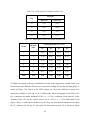
Table 2.1 – Fusion Stages & Techniques (Smith & Singh, 2006; Hall, 1992)
Fusion Stages
1. Data Alignment
Techniques
Coordinate Conversion
Nearest Neighbor
Joint Probabilistic Data Association
2. Data Association
Lagrangian Relaxation
Artificial Neural Networks
Fuzzy Logic
Kalman Filter
Particle Filter
3. Position Estimation
Multiple Model Algorithms
Multiple Resolutional Filtering
Artificial Intelligence Approaches
Bayesian Inference
Dempster-Shafer (D-S) Rule
4. Identity Estimation
Artificial Neural Networks
Expert Systems
Voting and Summing Approaches
Distributed Classification
Grewal & Andrews (2008) discussed that within the domain of MSDF, KF is exclusively used
for two purposes: 1) estimation, and 2) performance analysis of sensors. For estimation; KF
allows to estimate the state of dynamic systems with certain types of random behavior by using
information from sensory sources; while for performance analysis of sensors, KF helps to
determine which type of sensors would perform better for a given set of design criteria. These
criteria are typically related to estimating accuracy and system cost.
28
2.7 Applications of Multi-Sensor Data Fusion
MSDF has numerous industrial applications. This section mainly discusses the MSDF
applications in the domain of construction management. Some other applications of MSDF are
also discussed in this section.
2.7.1 Applications in Construction Management
The impact of data imperfections on construction process monitoring and the benefits of the data
fusion approach for construction management have been investigated by several researchers. Luo
et al. (2013) explored the effects of location-aware sensor data imperfections (e.g. erroneous or
missing data) on the autonomous jobsite safety monitoring and investigated methods to reduce
the impacts of the sensor data imperfections on the jobsite safety system. They found that the
imperfections of the location data collected from various location-aware sensors strongly affects
the safety monitoring system. Furthermore, they suggested the data fusion approach to reduce the
sensor data imperfections and to improve the performance of the jobsite safety monitoring
system.
Chi & Caldas (2012) presented an automated image-based safety assessment method for
earthmoving and surface mining operations. They evaluated the image-based data collection
devices and algorithms for safety assessment and also discussed the analysis techniques and rules
for monitoring the safety violations. They found that the applied safety rules enabled automated
violation detection and the utilization of the collected data was useful for safety decision-making.
However, they suggest that the image-based safety assessment method has some limitations
which can be overcome by integrating tracking devices, such as UWB or GPS, with the imagebased safety assessment method.
Shahi et al. (2012) incorporated a UWB RTLS system to track activities in a construction project
in order to automate the estimation of the construction projects’ progress. Although the scope of
their research was limited to ductwork, HVAC, and piping activities on the project, but their
proposed model is scalable to a complete construction project. Also, they showed a comparison
of concrete, steel, and piping projects and noted that the number of changes occurring during
construction may be significantly higher for piping and industrial projects in comparison to steel
or concrete building construction. They also found that although automated object recognition
29
and material tracking techniques, that use the 3D Computer-Aided Design (CAD) or Building
Information Modeling (BIM) model as a-priori information, may be accurate for concrete or steel
structures, they may be ineffective for tracking the progress of piping and many other
mechanical and electrical services carried throughout most of the projects.
El-Omari & Moselhi (2011) integrated various automated data acquisition technologies to collect
data from construction sites required for progress measurement purposes. They proposed a
layout of an IT platform, designed to facilitate automated data acquisition from construction sites
to support efficient time and cost tracking and control of construction projects. Furthermore, they
assessed the suitability of various automated data acquisition technologies, i.e. bar coding, Radio
Frequency Identification (RFID), 3D laser scanning, photogrammetry, multimedia, and penbased computers, for their use in tracking and controlling construction activities. They also
proposed a model that integrates with the automated data acquisition technologies, a planning
and scheduling software system, a relational database, and using AutoCAD to generate progress
reports that can assist project management teams in decision making.
Razavi & Haas (2010) studied the MSDF approach for on-site materials tracking in construction.
They used a data fusion model in an integrated solution for automated identification, location
estimation, and dislocation detection of construction materials. The data sources considered for
their MSDF model were various physical sensors, different location estimation algorithms,
location contexts from automated data collection technologies (Received Signal Strength
Indicator, Positional Dilution of Precision), time and BIM (site map/layout and drawings, 3D
models). Their particular focus was dislocation detection as it can be used to detect multihandling of materials. They applied Dempster-Shafer theory to the materials dislocation
detection and found this method is well-suited for this problem where both uncertainty and
imprecision are inherent to the problem. They also found that data fusion helps to improve the
accuracy and precision of the location estimations. They also indicated the potential for the
proposed model to improve location estimation and movement detection.
Rebolj et al. (2008) also presented an automated construction activity monitoring system based
on a combined method, consisting of three components: image recognition based tracking, BIM
based material tracking, and a communication environment supporting mobile computing. They
30
found that the proposed concept is capable of ensuring timely information for well-timed
reactions to unexpected events on construction sites.
Moreover, the MSDF approach has also been investigated for indoor security surveillance by
Rafiee et al. (2013). They presented a fully automated indoor security solution for intruder
tracking that fused data from three data sources, i.e. UWB RTLS, surveillance cameras and BIM.
They found that the MSDF approach is suitable for indoor security applications and also
appropriate for other types of applications. Dibitonto et al. (2011) also proposed a hybrid people
tracking system based on the fusion of data from UWB and computer vision, to achieve better
accuracy and reliability for people tracking.
2.7.2 Other MSDF Positioning Applications
Lundquist (2011) fused information from various sensors for estimating the motion of a vehicle
and the characteristics of its surroundings. He studied and compared various maps, in particular,
road maps which make use of the fact that roads are highly structured and allows relatively
simple and powerful models to be employed. He showed how the information of the lane
markings, obtained by a front looking camera, can be fused with inertial measurement of the
vehicle motion and radar measurements of vehicles ahead to compute a more accurate and robust
road geometry estimate. Furthermore, he showed how radar measurements of stationary targets
can be used to estimate the road edges, and applied a special filter to the radar data for
constructing a representation of the map of the stationary objects around the vehicle. For tracking
moving targets, he focused on the extended targets, i.e., targets which potentially may give rise
to more than one measurement per time step. He also introduced a framework to track the size
and shape of a target.
Ciftcioglu et al. (2007) described sensor data fusion in autonomous perceptual robotics. They
represented a visual perception by a probabilistic model, where the model receives and interprets
visual data from the environment in real-time. The perception obtained, in the form of 2D
measurements, is used for the robot navigation. They processed the visual data in a multiresolution form via wavelet transform and optimally estimated via EKF in each resolution level
and fused the outcomes for improved estimation of the trajectory. Their proposed approach not
only performs a vision task in a robot but also provides it with a simulated human vision.
31
Gustafsson et al. (2002) developed a framework for positioning, navigation, and tracking
problems using particle filters, which consists of a class of motion models and a general
nonlinear measurement equation for the position. They presented a general algorithm, which is
parsimonious with the particle dimension. They described how the technique of map matching is
used to match an aircraft’s elevation profile to a digital elevation map, and a car’s horizontal
driven path to a street map. They showed that the accuracy in both cases is comparable with
satellite navigation (e.g. GPS) but with higher integrity. They also argued, based on their
simulations, how the particle filter can be used for positioning based on cellular phone
measurements, for integrated navigation in aircraft and for target tracking in aircraft and cars.
2.8 Summary
The literature review presented in this chapter focused on the UWB RTLS and MSDF
technologies and their applications specifically in the domain of construction management. UWB
RTLS is an effective technology for localizing construction equipment on construction sites.
Several researchers have investigated the applicability of UWB RTLS for construction
management; however, a thorough examination of the wireless UWB system for real
construction environment is missing in the literature. Moreover, two data enhancement methods
are also reviewed which would be used to minimize the erroneousness of the UWB data.
Furthermore, it was found that several researchers have studied fusion of data from multiple
sources for various aspects of construction management; and their study showed that this
technique has strong potential in the domain of construction management.
Pertaining to the limitations of the UWB technology and the potentials of the MSDF technology,
we propose MSDF based approach for localization of construction equipment. We believe that
the combined usage of the UWB technology with the image processing based equipment
detection and localization can effectively locate construction equipment on construction sites by
applying an accurate data fusion model.
32
CHAPTER 3
EXPERIMENTAL PERFORMANCE ANALYSIS
OF UWB RTLS
3.1 Introduction
As discussed in CHAPTER 2, several researchers investigated the performance of the UWB
RTLS for construction projects. However, a comprehensive research that analyzes the
performance of the UWB system, specifically wireless, under dynamic conditions in both indoor
and outdoor environments is missing in the literature. Thus, the objectives of this chapter are to:
(1) evaluate the factors that affect the performance of the UWB system, (2) analyze and compare
the performance of the wired and the wireless UWB systems for indoor environments in a
dynamic mode, and (3) evaluate the performance of the wireless UWB system for outdoor
construction environment under dynamic conditions.
This chapter is organized as follows: The factors that affect the performance of the UWB system
are discussed in Section 3.2; Section 3.3 demonstrates the indoor and outdoor dynamic
experiments which were conducted to analyze the performance of the UWB system for
construction projects; and the conclusions and recommendations are presented in Section 3.4.
3.2 Factors affecting the UWB System’s Performance
Setting up a UWB system requires several crucial steps including the placement of sensors,
measuring the coordinates of sensors, configuration of network connection, and configuration of
various software components. These steps are detailed in Appendix A. Furthermore, the settings
of the wired and the wireless UWB systems are not similar, as shown in Figure 2.4. For the
wired system (Figure 2.4(a)), all sensors are connected with each other through Ethernet cables
for the estimation of TDoA and all sensors are also connected to a network switch for the
communication of sensors with the server. Whereas for the wireless system (Figure 2.4(b)), each
sensor is connected to the wireless bridge in order to communicate with the computer server.
Several factors affect the performance of the UWB system, which are listed in Table 3.1. In
terms of system settings, the wireless system is more critical than the wired system. As for the
wired system, all sensors are connected through the timing and data cables, whereas for the
33
wireless system, appropriate settings of wireless bridges are essential because of the additional
issues related to the stability of the communication between the sensors. The RF power and RF
frequency of the wireless bridges should be selected according to the environment, as the RF
frequency might receive interference from the existing Wi-Fi networks. The effect of wireless
bridges is investigated in detail in Section 3.3.2.1.
It is also important to select the right type of tags for each environment. The compact tags are
suitable for tracking equipment, whereas for workers, slim tags are preferable. Furthermore,
appropriate tag settings can improve the performance of the UWB system. The update rate of
tags is critical and should be selected based upon the total number of tags present in the UWB
covered area. For the UWB system used in this research (Ubisense, 2013), each second is
divided into 153 time slots where the length of each time slot is 7.453 msec. The highest update
rate which can be selected is 33.54 Hz which requires four time slots (Slot Interval = 4). To
achieve this update rate, a maximum of four tags should be present in the UWB covered area. As
the number of tags increases, the update rate will decrease in order to allow the system to log all
tags’ location. For example, if the update rate is set to maximum but eight tags are present in the
UWB covered area, the update rate would automatically be decreased to 16 Hz. Another concern
when setting the update rate is the moving velocity of the tagged objects. Objects with high
velocity need more frequent updates to accurately track their traces. Therefore, it is essential to
select a suitable number of tags with an appropriate update rate based upon their velocity (Zhang
et al., 2012a). Equation (3.1) presents the formula for calculating update rate.
(3.1)
Strategic placement of tags is also very important, as elevated tags yield better performance
(Maalek & Sadeghpour 2013, Saidi et al. 2011) and the phenomenon of Dilution of Precision
also has a strong impact on the location accuracy, as explained in Section 2.3 (Maalek &
Sadeghpour 2013). Another significant factor related to tag settings is filtering. The data from the
UWB sensors are filtered to remove the noise and minimize the location errors. The UWB
system, used in this research, supports four types of Information Filters (IF) which estimate a
tag’s current position by using its previous motion (Ubisense, Location Engine Configuration
User Manual, 2013a). The four variants of IF are: (1) information filter; (2) fixed height
34
information filter; (3) static information filter; and (4) static fixed height information filter. Each
variant of the IF has a number of parameters that control the behavior of the filter, out of which
12 parameters are common to all types of IF. One of the 12 common parameters is Minimum
Reset Measurements (MRM) which represents the minimum number of supporting
measurements required. A single measurement can be either an azimuth, an elevation, or a
TDOA between two sensors (Ubisense, 2013). In the wired setting, if two sensors see a tag, there
will be five measurements (azimuth and elevation from each sensor, plus a TDOA) whereas in
the wireless setting, if two sensors see a tag, there will be four measurements (just the azimuth
and elevation from each sensor), as there is no TDOA in the wireless setting.
Another important factor that affects the overall performance of the UWB system is the number
of UWB sensors used to monitor the area. Table 3.2 summarizes the effect of number of sensors
and location method on the UWB system’s performance. It can be observed that for the wireless
UWB system (AOA only), as the number of sensors increases (2 or more), the system would be
able to estimate the location of tags more accurately; and with only one sensor, the system can
only provide 2D position without extra information. However, for the wired system (TDOA +
AOA), two sensors are enough for a good 3D location accuracy. Moreover, the size and
geometry of the sensor cell are very critical. It is preferable that the sensor cell would be in a
square-like geometry. If a sensor cell has a poor geometry, the accuracy of the estimated
locations would be affected. The performance of the UWB system is also sensitive to the
orientation and the measurement of the locations of sensors and the location of the calibration
tags.
Finally, it is essential to assess the environment where the UWB system would be used. The RF
noise present in the environment could affect the accuracy of estimated locations. Furthermore,
the materials of objects which are to be tagged and the objects which are present in the
environment have impact on the performance of the UWB system.
35
Table 3.1 – Factors affecting UWB System
Category
Wired
Factor
Cable connections
Line of sight between bridges
Connection-typedependent
RF frequency of bridges
Wireless
RF power of bridges
Distance between bridges
Compact
Tag Type
Slim
Expected update rate vs. Actual update rate
Filtering algorithm and parameters
Tag Settings
Total number of tags used in the test
Strategic placement of tags (elevated tag gives better
result)
Dilution of Precision
Connection-typeindependent
Number of sensors
System
Settings
Size and geometry of cell
Measurement of location and orientation of sensors
Quality of calibration and measurement of location of Tag
RF Noise
Object to be tagged (Metallic/Non-metallic/Humans)
Environment
Objects present in the monitored area
(Metallic/Liquid/Humans)
Line of Sight between sensors and tags
36
Table 3.2 – Effect of Number of Sensors on the UWB System (adapted from Zhang, 2010)
Location method
Number of sensors
detecting tag
Extra information
required
AOA
1
Known height of tag
AOA
2 or more
None
3D position
TDOA+AOA
2 or more
None
3D position (highest
accuracy)
Result
2D horizontal position
(+ known height)
3.3 Experimental Work
The performance of the UWB system for construction management is evaluated by conducting
three indoor and three outdoor tests. Furthermore, the performances of the wired and the wireless
UWB systems are also compared by conducting two sets of indoor tests. These indoor and
outdoor tests are summarized in Table 3.3 and discussed in detail in the following sections.
Table 3.3 – Overview of Experimental Work
Location
Indoor
Outdoor
UWB System
Purpose
Data Processing
EUR (Hz)
Wireless
Evaluation of
Tags’ Performance
No
16
Wired and
Wireless
Performance
Comparison
SCM
34
Wired and
Wireless
Performance
Comparison
Simple Averaging
4.19
Wireless
Tracking Real
Excavator
N/A
8.3
Wireless
Tracking Real
Roller
SCM and OM
8.3
Wireless
Tracking Real
Excavator
Simple Averaging
4.19
37
3.3.1 Indoor Dynamic Tests
3.3.1.1 Indoor Wireless Dynamic Test to Evaluate Performance of Tags
Design of Experiment
This test was conducted at the atrium of the 5th floor of the Engineering and Visual Arts
Complex (EV) building of the Concordia University’s Downtown campus. The objectives of this
test were to: (1) evaluate the performance of the wireless UWB system for indoor security
applications, and (2) evaluate the performance of the two types of the UWB tags, which are the
compact tags and the slim tags (Figure 2.1).
Four persons were involved in this test, each having two UWB tags; one compact and one slim.
Table 3.4 lists the IDs of the tags used by each person and Figure 3.1(a) shows the position of the
tags carried by each person. It can be observed from Figure 3.1(a) that the slim tag was placed
near the body of the person whereas the compact tag was kept slightly away from the body; also
the compact tag was slightly more elevated than the slim tag. The Expected Update Rate (EUR)
of the tags was set to 16 Hz because only 8 tags were present in the monitored area. The data
were collected for 3 minutes. Static Information Filtering (SIF) was used with the value of MRM
set to 5.
The covered area by the UWB sensors was 8.48 m x 8.72 m, as shown in Figure 3.2. As this test
was conducted using the wireless UWB system, so the UWB sensors were connected to the
wireless bridges, as shown in Figure 3.1(b). Figure 3.1(c) and Figure 3.1(d) show the positions of
UWB sensors in the monitored area. Video of the test was also recorded using a Sony IP PTZ
Camera as an extra source of information to validate the UWB results.
Table 3.4 - Tag IDs
Person
Tag IDs
Slim
Compact
P1
010-000-084-205
020-000-101-222
P2
010-000-084-202
020-000-108-122
P3
010-000-084-228
020-000-059-088
P4
010-000-084-195
020-000-059-098
38
Compact Tag
UWB Sensor
Slim Tag
Wireless Bridge
(a) Tag Positions
(b) Sensor & Wireless Bridge
Sensor 1 (Master)
Workstation
Sensor 3
Sensor 4
Sensor 2
(c) Position of Sensor 1 & 2
(d) Position of Sensor 3 & 4
Figure 3.1 – Test Settings
Performance Analysis
For analyzing the performance of the wireless UWB system and comparing the performance of
the slim tags with the compact tags, firstly, the Actual Update Rate (AUR) and the Missing Data
Rate (MDR) of all tags were analyzed. The AUR and the MDR are calculated using Equations
(3.2) and (3.3), respectively. In Equation (3.2), Δt is the time difference between two consecutive
readings.
39
(3.2)
(3.3)
Origin
(0, 0, 0)
8.48 m
Y
Sensor 1
X
Sensor 2
8.72 m
UWB Covered Area
Sensor 3
Sensor 4
Figure 3.2 - Area Settings
Table 3.5 lists the AUR and MDR of both types of tags for each person. It can be observed that
the AURs are different from the EUR, which was 16 Hz. Especially for the compact tags, the
maximum AUR is 2.44, with an MDR of 84.88 %, for P2 which is considerably lower than the
EUR, whereas for the slim tags, the maximum AUR is 12.99, with an MDR of 19.25 %, for P2.
40
It is prominent that the AUR of compact tags is considerably lower than that of slim tags and
their MDR is also much higher than that of the slim tags. Therefore, in terms of AUR and MDR,
the slim tags have better performance than the compact tags. One reason for this lower
performance can be that the compact tags have omnidirectional antenna but the slim tags have
unidirectional antenna; and the compact tags were held in a position that they were not facing the
sensors rather they were facing up, whereas the slim tags were facing the sensors.
Table 3.5 – Update Rate and Missing Data Rate Analysis
Person
Actual Update Rate (Hz)
Missing Data Rate (%)
Slim Tags
Compact Tags
Slim Tags
Compact Tags
P1
8.82
2.36
45.19
85.32
P2
12.99
2.44
19.25
84.88
P3
10.66
2.17
33.70
86.59
P4
12.34
2.28
23.22
85.82
Moreover, the movements of the four persons, estimated by both tags, were analyzed. Figure 3.3
shows the movement of P1, which was almost in a straight path along the vertical axis. By
comparing Figure 3.3(a) and Figure 3.3(b), it can be observed that although both tags were in
close vicinity, but the movements estimated by both tags are very much different; the reason for
this might be the antenna type and the direction of tags as discussed earlier in this section. The
movement of P2 was also almost in a straight path but along the horizontal axis, as shown in
Figure 3.4, while P3 was moving almost in a circular path, as shown in Figure 3.5. Figure 3.6
shows the movement of the P4, who was moving randomly without following a specific path.
41
7
7
6
6
5
5
4
4
3
3
2
2
1
1
0
0
3
4
5
6
7
3
4
(a) Slim Tag
5
6
7
(b) Compact Tag
Figure 3.3 - Tag's Performance Comparison for P1
7
7
6
6
5
5
4
4
3
3
2
2
2
3
4
5
6
7
2
(a) Slim Tag
3
4
5
(b) Compact Tag
Figure 3.4 - Tag's Performance Comparison for P2
42
6
7
7
7
6
6
5
5
4
4
3
3
2
2
1
1
1
2
3
4
5
6
7
8
9
1
2
(a) Slim Tag
3
4
5
6
7
8
(b) Compact Tag
Figure 3.5 - Tag's Performance Comparison for P3
5.5
5.5
4.5
4.5
3.5
3.5
2.5
2.5
1.5
1.5
3
4
5
6
7
3
(a) Slim Tag
4
5
6
7
(b) Compact Tag
Figure 3.6 - Tag's Performance Comparison for P4
3.3.1.2 Indoor Dynamic tests to compare Performance of Wired and Wireless Systems - I
In order to compare the performance of wired UWB system with the wireless UWB system, two
sets of indoor dynamic tests were conducted, with two tests in each set. These tests, in which the
movement of a remote-controlled (RC) crane was tracked, were conducted in a lab environment.
43
9
Design of Experiment
The Design of Experiment (DoE) for both set of tests was kept the same in order to simplify the
performance comparison of both systems. The boom of the RC-crane was moved in a circular
path around its center of rotation. The ground truth was the controlled movement of the RCcrane from which the center point and the radius of the circle were measured. Furthermore, it
was analyzed whether the tracked movement of the boom of the RC-crane was smooth or not.
Figure 3.7 shows the UWB area settings for these tests. The first set of tests was conducted with
the wired UWB system whereas the second set was conducted with the wireless system. Within
each set, the first test was conducted with the RC-crane placed at the center of the UWB covered
area (see Position A in Figure 3.7), as described in Table 3.6, while in the second test, the RCcrane was placed near the edge of the UWB covered area (see Position B in Figure 3.7) to
evaluate the impact of the phenomenon of DoP, as discussed in Section 3.2, and the effect of the
surrounding objects at the two locations. Furthermore, in each test the RC-crane was elevated
from the ground by almost 1 meter in order to improve the location accuracy, as discussed in
Section 3.2.
Table 3.6 – Description of Indoor Dynamic Tests – I
Test Name
UWB System
Position
1A
Wired
A
1B
Wired
B
2A
Wireless
A
2B
Wireless
B
The same tags were used in both set of tests and their EUR was set to the maximum, i.e. 34 Hz,
as only three tags were present in the UWB covered area. For filtering, SIF was used in which
the value of MRM was set to 5 for the wired tests whereas for the wireless test, its value was set
to 3.
These tests were conducted using the following steps: (1) Attach three tags to the tip of the boom
of RC-crane; (2) Place the RC-crane on a cart of height 0.9 m, and position it so that the 2D
coordinates of the center of rotation of boom would be (2.35, 3.30) for tests 1A and 2A, and
44
(2.18, 0.91) for tests 1B and 2B; (3) fully extend the boom of the RC-crane; (4) position the
boom to position 0 (see Figure 3.8); (5) rotate the boom clockwise until it reaches position 1; (6)
rotate the boom anti-clockwise until it reaches position 2.
4.16 m
Sensor-2
Metallic Whiteboard
X
Sensor-1 [M]
Position B
Y
Switch
7.32 m
Door
Position A
Sensor-3
Timing Cable
Sensor-4
Sensor with orientation (yaw)
Data Cable
Figure 3.7 – Area Settings for Indoor Dynamic Tests – I
Performance Comparison of Wired and Wireless UWB Systems
Initially, the consistency of the logged data is analyzed for both set of tests. Table 3.7 shows the
AUR and MDR of all three tags for both sets of tests. From Table 3.7, it can be observed that the
performance of the wired system is quite reasonable whereas the wireless system’s results are
poor. In the two tests with the wired system, i.e. 1A and 1B, each tag’s AUR is very close to the
45
EUR, and the MDR is relatively low. For example, the maximum MDR is 29.26 of Tag 1 in test
1A. However, in the tests with the wireless system, i.e. 2A and 2B, the AUR is considerably
lower than the EUR, and the MDR is high. In test 2A, no data was logged for Tag 1 and for the
other two tags; the AUR is low, whereas in test 2B, the MDR for tag 3 is almost 88%. It can be
noted that for all two tests with the wireless system, for all tags the MDR is more than 50%.
Position 2
Tags
Position 1
Position 0
Figure 3.8 – Design of Experiment for Indoor Dynamic Tests - I
Table 3.7 – AUR and MDR Analysis for Indoor Dynamic Tests - I
1A
1B
2A
2B
Tag
AUR
(Hz)
MDR
(%)
AUR
(Hz)
MDR
(%)
AUR
(Hz)
MDR
(%)
AUR
(Hz)
MDR
(%)
1
24.05
29.26
32.31
6.92
0.00
100.00
17.10
69.41
2
28.85
15.16
29.97
13.59
15.50
56.28
16.83
54.61
3
30.05
11.61
31.44
9.30
8.23
76.40
20.57
88.04
Furthermore, to analyze the movement of the RC-crane’s boom, each tag’s data were firstly
averaged over a period of 500 msec and then the data of the three tags were averaged. In case of
the wireless test (i.e. 2A), only data from tag 2 and tag 3 were averaged as no data were logged
from tag 1. The tracked rotational movement of the boom of the RC-crane is shown in Figure
3.9(a) and Figure 3.9(b). In these figures, the red circle shows the expected path of the RCcrane’s boom and the black line shows the actual movement of the RC-crane’s boom as localized
by the UWB system. From Figure 3.9(a), it can be observed that the movement of the boom of
the RC-crane, as tracked by the wired system, followed a linear pattern. However, in contrast,
boom’s movement tracked by the wireless system is too noisy and it cannot be certainly
concluded that which path was followed by the boom (Figure 3.9(b)).
46
To further improve the accuracy of the data, SCM is applied to the data collected from these
tests. For applying SCM, one OC and three GCs were considered, which are described in Table
3.8. The speed of rotation of boom is 13.3°/sec (Zhang, 2010) which is converted from °/sec to
m/sec using Equation (3.4), where r is the radius of rotation and its value is 0.66 m.
(3.4)
Table 3.8 – OC and GCs for Indoor Dynamic Tests - I
Constraint
OC
Description
Speed of rotation of boom
Value
0.16 m/sec
GC 1
Distance between Tag 1 and Tag 2
4 cm
GC 2
Distance between Tag 2 and Tag 3
8 cm
GC 3
Distance between Tag 1 and Tag 3
4 cm
The results of the SCM are shown in Figure 3.9(c) and Figure 3.9(d). From Figure 3.9(c), it can
be observed that the SCM has not enhanced the data from the wired UWB system, whereas from
Figure 3.9(d), it is clear that the data from the wireless UWB system is enhanced by the SCM.
This is because the data from the wired system was already good.
Moreover, the accuracy of the tests 1A and 1B is analyzed and compared, as shown in Table 3.9.
For calculating the accuracy, the mean difference between the radii of the expected rotation and
the UWB estimated rotation is calculated and analyzed along with its standard deviation. It can
be observed that for the wireless system, the SCM has improved the accuracy whereas for the
wired system, the SCM has not produced better results.
Therefore, in view of the analysis presented in Figure 3.9, Table 3.7, and Table 3.9, it is
concluded that for indoor applications, the wired system performs much better than the wireless
system, and the SCM has the potential to improve the accuracy of the data collected from the
wireless UWB system.
47
4
4
3.5
3.5
3
3
2.5
2.5
1.5
2
2.5
3
1.5
(a) 1A - Averaged
2
2.5
3
(b) 2A - Averaged
4
4
3.5
3.5
3
3
2.5
2.5
1.5
2
2.5
3
1.5
(c) 1A - SCM
2
2.5
3
(d) 2A - SCM
Figure 3.9: Performance Comparison of Wired UWB System and Wireless UWB System
Evaluation of Impact of Dilution of Precision
For evaluating the impact of DoP, the data collected from tests 1B and 2B are analyzed. For data
analysis, each tag’s data were firstly averaged over a period of 500 msec and then the data of the
three tags were averaged. In case of the wireless test (i.e. 2B), only data from Tag 1 and Tag 2
were averaged as the MDR of Tag 3 is almost 88% (see Table 3.7). The tracked rotational
movement of the boom of the RC-crane is shown in Figure 3.10. Figure 3.10(a) shows the data
48
from tests 1A and 1B, where Figure 3.10(b) shows the data from tests 2A and 2B. It can be
observed that the in tests 1A and 2A, the RC-crane was in the middle of the UWB covered area
(corresponding to Position A in Figure 3.7) whereas the in tests 1B and 2B, the RC-crane was
near the edge of the UWB covered area (corresponding to Position B in Figure 3.7). From Figure
3.10(a), it can be observed that in both positions, the performance of the wired UWB system is
comparable. However, in contrast, the performance of the wireless system varies with respect to
the position of the tracked object, as shown in Figure 3.10(b). Similar conclusion can be drawn
by comparing the AUR and MDR of these tests presented in Table 3.7. The AUR and MDR of
tests 1A and 1B are somehow similar whereas for tests 2A and 2B, the performance of the
wireless UWB system, in terms of AUR and MDR, is better when the RC-crane was at Position
B. From this analysis, it is concluded that the phenomenon of DoP does not strongly affect the
performance of the wired UWB system in indoor environments; however the performance of the
wireless UWB system is affected by DoP. One reason for this difference in performances is that
the wireless UWB system only uses AoA technique to estimate the position of the tagged object,
and when the tagged object is not in the middle of the UWB covered area, then the estimation
based on angles is not accurate; whereas, the wired UWB system estimates using TDoA
technique in addition to the AoA technique, so the angle calculation is affected by DoP but the
calculation based on time difference can produce accurate results.
Table 3.9 – Accuracy Analysis for Tests 1A and 2A
Standard deviation of radius difference
(cm)
Mean radius difference (cm)
Tag
1A
(without
SCM)
1A
(with
SCM)
2A
(without
SCM)
2A
(with
SCM)
1A
(without
SCM)
1A
(with
SCM)
2A
(without
SCM)
2A
(with
SCM)
Tag 1
18.12
17.12
N/A
N/A
8.58
8.55
N/A
N/A
Tag 2
16.84
15.69
22.89
12.88
10.63
8.82
23.56
10.51
Tag 3
14.18
18.01
12.25
20.09
9.71
8.60
3.67
10.57
Averaged
16.66
16.98
16.69
16.04
8.47
8.58
11.34
10.31
49
4
4
2A
1A
3
3
2
2
2B
1B
1
1
0
0
0
1
2
3
4
0
(a) Wired UWB System
1
2
3
4
(b) Wireless UWB System
Figure 3.10 – Investigation of Impact of Dilution of Precision Phenomenon
3.3.1.3 Indoor dynamic tests to compare performance of Wired and Wireless Systems –
II
Design of Experiment
Two sets of tests were designed to compare the performance of the wired UWB system with the
wireless UWB system. Within each set, the DoE for both tests was kept the same in order to
simplify the performance comparison of both systems. These sets of tests were conducted in the
atrium of the 8th floor of the EV building in Concordia University’s downtown campus. In each
set, one test was conducted with the wired UWB system, whereas the other test was conducted
with the wireless UWB system. The UWB covered area was 7.7 m x 5.7 m, as shown in Figure
3.11.
In the first set of tests, the movement of a person was tracked who was carrying two compact
tags and was following a pre-defined path (shown as A in Figure 3.11) whereas in the second set
of tests, the movement of a compact tag was tracked which was moved on a pre-defined inclined
straight line (sloping rope shown as B in Figure 3.11) where one end of the rope was about 2
meters above the ground and the other end was at the ground.
50
In both set of tests, the EUR of the tags was set to 4.19 Hz as 32 tags were present in the
monitored area, and the SIF was used with the value of MRM set to 5 and 3 for the wired and
wireless systems, respectively.
Sensor 4
A (Path followed by the person)
Sensor 3
B (Inclined path for tag)
7.7 m
Y
UWB Covered Area
Origin Sensor 1
(0, 0, 0)
X
Sensor 2
5.7 m
Figure 3.11 - Area Settings for Indoor Dynamic Tests - II
51
Performance Comparison
At first, the first set of tests is analyzed in which the movement of a person is tracked. For this
set, primarily the consistency of logged data is analyzed. Table 3.10 presents the AUR and MDR
analysis for this set. It can be noted that for the wired system, the AUR is almost the same as
EUR for both tags and the MDR is also 0%. Whereas in the case of the wireless system, the
AUR is slightly less than the EUR and some data are missing.
Table 3.10 – AUR and MDR Analysis for Indoor Dynamic Tests - II
Tag
Wired
Wireless
AUR (Hz)
MDR (%)
AUR (Hz)
MDR (%)
1
4.19
0
3.85
9.37
2
4.18
0
3.88
8.40
To further analyze each tag’s performance with respect to location accuracy, the paths based on
raw data are drawn for each tag, as shown in Figure 3.12. In this figure, the black line shows the
locations of tag estimated by the UWB system whereas the red line shows the actual path
followed by the person. By comparing Figure 3.12(a) and Figure 3.12(c), it can be observed that
for tag 1, the wired system has estimated fairly good locations while the locations estimated by
the wireless system are too noisy. Similar observation can be made about tag 2 by comparing
Figure 3.12(b) and Figure 3.12(d).
To further improve the location of the person estimated by the wired and the wireless UWB
systems, the data collected from these tests are enhanced by firstly averaging each tag’s data over
a period of 1 sec and then the data of both tags were averaged. Figure 3.13 shows the tracked
paths of the person after the aforementioned processing. By comparing Figure 3.13(a) and Figure
3.13(b), it can be observed that after the processing, the paths of the person tracked by the wired
system is more accurate than the paths tracked by the wireless system. Furthermore, the data
from the wireless system are still noisy.
52
6
6
5
5
4
4
3
3
2
2
1
1
2
3
4
5
2
(a) Wired - Tag 1
3
4
5
(b) Wired - Tag 2
6
6
5
5
4
4
3
3
2
2
1
1
1.5
2.5
3.5
4.5
1.5
(c) Wireless - Tag 1
2.5
3.5
(d) Wireless - Tag 2
Figure 3.12 - Wired and Wireless UWB System – II – Raw Data
53
4.5
6
6
5
5
4
4
3
3
2
2
1
1
2
3
4
5
2
(a) Wired
3
4
5
(b) Wireless
Figure 3.13 – Wired and Wireless UWB System – II – Averaged Data
The performance of the systems is compared for the second set of tests related to a tag sliding on
the sloped rope. Initially, the consistency of the logged data is analyzed and presented in Table
3.11. It can be observed that for both systems, i.e. wired and wireless, the AUR is almost the
same and is slightly less than the EUR. One reason for the low AUR and high MDR of the wired
system can be that the start point of the movement of the tag was actually out of the UWB
covered area (see Figure 3.11).
Table 3.11 – AUR and MDR Analysis for Slope Test
Tag
1
Wired
Wireless
AUR (Hz)
MDR (%)
AUR (Hz)
MDR (%)
3.77
8.98
3.86
7.09
54
The raw data from these two tests were plotted, as shown in Figure 3.14. From this figure, it is
clear that the movement of the tag on the slope is more realistically captured by the wired
system; whereas for the case of the wireless system, the data are too noisy.
4.5
4.5
4
4
3.5
3.5
3
-1.5
3
0.5
2.5
4.5
-1.5
(a) Wired
0.5
2.5
4.5
(b) Wireless
Figure 3.14 – Wired and Wireless UWB System – II – Slope – Raw Data
3.3.2 Outdoor Dynamic Tests
3.3.2.1 Outdoor dynamic test for tracking movement of an excavator
Design of Experiment
This test was conducted on the intersection of two busy streets, i.e. Saint Catherine and Guy, in
Downtown Montreal. This test was designed to: (1) evaluate the performance of the wireless
UWB system in outdoor environment, and (2) investigate whether tags are easily attachable to
construction equipment using magnets.
Each UWB sensor was connected to the wireless bridges and they both were installed on a
tripod, as shown in Figure 3.15. Compact tags were prepared for attaching them to equipment by
adding two magnets with each tag, as shown in Figure 3.16. These tags were then attached to the
excavator, as shown in Figure 3.17.
Results
Although the system was configured properly, this test was not successful because the UWB
system was unable to detect the tags. It was found that the connectivity between sensors was
intermittent. Sometimes the sensors were connected and sometimes they were not. One reason
55
for the connectivity issue can be the interference from Wi-Fi signals of nearby coffee shops. The
wireless bridges were operated at 2.4 GHz radio frequency with 25% RF power.
Lessons Learned
Through this experience, it was learned that the wireless bridges should be operated at 5 GHz
radio frequency, so that the connectivity is not affected by other wireless systems, and the power
level should be adjusted according to the site layout and site conditions.
Furthermore, it was also concluded that the tags were easily attachable to the equipment using
magnets and they did not cause any problem during the operation of equipment.
UWB Sensor and
Wireless Bridge
Wireless
Access Point
Work
Station
Figure 3.15 – UWB Settings for Outdoor Test
56
Figure 3.16 – Compact tags with magnet for Construction Equipment
Tag
Tag
(a) Right
(b) Left
Figure 3.17 – Tag positions on excavator
Investigation of the Effect of Wireless Bridges
As the results of this test were not satisfactory, therefore another set of tests was conducted to
evaluate the impact of wireless bridges on the overall performance of wireless UWB system. In
this set of tests, the wireless bridges are tested in indoor and outdoor scenarios, with varying
distances and obstacles. The indoor test was conducted on the 8th floor of the EV building
57
(Concordia University’s Downtown Campus), which contains drywalls, concrete structure and
concrete stairs, whereas the outdoor test was conducted at a busy street in Downtown Montreal.
The results of the indoor test are presented in Table 3.12. It can be observed that at shorter
distances, i.e. less than 15 m, the system works properly without line of sight but as the distance
increases, the connectivity is not possible with thick obstacles, which are normally present in the
indoor environment. In this test setting, at the distance of 27.5 m, the bridge and access point
were separated by some walls and stairs which include steel and concrete; whereas, with
complete line of sight, the connectivity is good up to a distance of almost 61 m.
Table 3.12 – Results of Indoor Wireless Connectivity Test
Distance
(m)
RF Power
(%)
Line of
Sight
Connectivity Status
11.5
25
No
Connected
25
27.5
50
Not Connected
No
100
Not Connected
Not Connected
33
25
Yes
Connected
61
25
Yes
Connected
The results of the outdoor test are presented in Table 3.13. It can be observed that the
connectivity is quite good up to a distance of almost 60 m whereas as the distance increases more
than 60 m, the connectivity is not reliable. In the case where the distance is 80 m, the bridge was
at one side of the street and the access point was at the other side and there was a truck between
the bridge and the access point.
3.3.2.2 Outdoor dynamic test for tracking movement of a roller
Design of Experiment
This test was designed to track the movement of a roller, which is operating on a construction
site. The duration of this test was 29.5 minutes. Four UWB sensors were installed at the edges of
the site covering an area of 22.98 m x 14.035 m, as shown in Figure 3.18. Although two tags are
enough for tracking the roller’s movement, four tags, i.e., S1, S2, S3 and S4, were attached to the
58
roller to provide data redundancy as shown in Figure 3.19(b). The EUR of tags was set to 8.3 Hz
as total 14 tags were present in the monitored area, and SIF was used with all the default settings
except MRM, which is set to 3 because of the wireless setting of the UWB system in this test.
Table 3.13 – Results of Outdoor Wireless Connectivity Test
Distance
(m)
RF Power
(%)
Line of
Sight
12.5
0.1
60
25
50
Connected
Yes
Connected
Connected
100
Connected
12.5
Not Connected
25
50
Yes
100
80
Connectivity Status
50
100
Connected
Connected
Connected
No
Not Connected
Connected
Performance Analysis
The data are analyzed in the 2D plane. For a better analysis, the duration of the test is divided
into six five-minute-long periods. The AUR of each tag is analyzed and presented in Table 3.14.
It can be observed that the AUR are very different from the EUR, tag S4 has the best
performance whereas tag S2 has the worst performance. Furthermore, firstly the MDR was
analyzed, as shown in Table 3.15. It can be observed that in this case, tag S2 has the worst
performance with an MDR of 73.91% whereas tag S4 has the best performance with an MDR of
23.93%. Then the MDR was analyzed at the second level, which means if the data is missing for
the whole second then it is considered as missing data. Table 3.16 shows the MDR analysis at
the second level. In view of the analysis presented in Table 3.14, Table 3.15 and Table 3.16, it is
concluded that the performance of tags S1 and S2 is unsatisfactory and, in contrary, the
59
performance of tags S2 and S3 is reasonable. One explanation of this is that having been placed
higher on the equipment, S3 and S4 had better visibility than S1 and S2.
22.98 m
Sensor 2
Sensor 3
14.035 m
UWB Covered Area
22.98 m x 14.035 m
Origin
Y
(0, 0, 0)
X Sensor 1
Sensor 4
Figure 3.18 – Area Settings for Outdoor Dynamic Test
S
S
4
3
S
S
2
1
(a) During Compaction Process
(b) Tag Positions
Figure 3.19 – Tracked Roller for Outdoor Dynamic Test
60
Table 3.14 – AUR Analysis for Outdoor Dynamic Test
AUR (Hz)
Tag
Real Test
Static Test
S1
2.34
8.29
S2
2.30
8.09
S3
4.53
8.31
S4
6.56
8.31
Table 3.15 – MDR Analysis (msec) for Outdoor Dynamic Test
Period
Duration
(min)
Missing Data Rate (%) - msec
S1
S2
S3
S4
1
5
70.96
64.86
42.09
23.21
2
5
76.10
66.02
44.54
20.76
3
5
56.59
83.01
55.58
17.55
4
5
73.41
72.45
39.36
14.58
5
5
79.76
76.51
41.85
31.20
6
4.5
80.63
80.59
62.52
36.28
Total
29.5
72.91
73.91
47.66
23.93
To further investigate each tag’s performance in terms of the logged data, control charts were
drawn for the time difference between two consecutive readings for the first 500 data points, as
shown in Figure 3.20. Based on the EUR settings, the ideal time difference between two
consecutive readings of each tag is 119.25 milliseconds, which corresponds to the EUR of 8.3
Hz. A minimum acceptable threshold of 50%, i.e., 4.15 Hz, is assumed for the interval. So the
Tolerance Limit (TL) for this control chart is set to 119.25 x 2 = 238.5 milliseconds. From
Figure 3.20(a), it can be observed that for tag S1, there are more than 40 data points exceeding
the TL, whereas also for tag S2, more than 40 data points exceeds TL as shown in Figure
61
3.20(b). From Figure 3.20(c), it can be observed that almost 40 data points exceeds the TL for
tag S3, while for tag S4, almost 20 data points exceeds TL (Figure 3.20(d)). Moreover, along
with the points exceeding TL, the maximum time difference between two consecutive readings is
also very critical. From Figure 3.20, it can be observed that tag S2 has the highest difference
between two consecutive readings which is 2756 msec and tag S4 has the best performance in
this regard.
To investigate whether or not the low update rate and the high ratio of missing data were because
of the performance of tags, a static indoor test was conducted using the same tags and same EUR
setting using the wired UWB System. Table 3.14 shows the AUR of the four tags for the static
test. It can be observed that the AUR for each tag is very much close to the EUR. Accordingly, it
can be observed that the tags are not the cause of the high MDR. This observation along with the
results of Section 3.3.1.2, where the wired and wireless systems were compared under exactly
the same condition, can suggest that the high MDR is an inherent limitation of the wireless UWB
system.
Table 3.16 – MDR Analysis (sec) for Outdoor Dynamic Test
Period
Duration
(min)
Missing Data Rate (%) - sec
S1
S2
S3
S4
1
5
37.33
31.00
10.33
6.33
2
5
44.33
34.67
13.33
3.00
3
5
23.67
23.00
17.67
2.00
4
5
46.67
34.67
7.67
3.00
5
5
43.67
41.00
11.33
11.33
6
4.5
27.41
35.56
16.67
2.22
Total
29.5
37.34
33.28
12.77
4.69
Figure 3.21 shows the cumulative probability of occurrence of the various update rates with
which the data was logged for each tag. This figure should be read from right to left. For
instance, it can be observed that, for tag S1, 90% of the data was logged with an update rate of
62
more than 2 Hz while 80% of the data was logged with an update rate of more than 4.3 Hz.
However, for tag S4, 90% of the data was logged with an update rate of more than 7.7 Hz while
80% of the data was logged with an update rate of more than 7.9 Hz. Similar analysis can be
observed for tag S2 and S3.
63
Time Difference
TL
Time Difference
EUR
Time Difference (msec)
Time Difference (msec)
2500
2500
2000
1500
1000
500
2000
1500
1000
500
0
0
0
100
200
300
Sequence of readings
400
-500
500
0
100
Time Difference
TL
EUR
Time Difference
2500
2500
Time Difference (msec)
3000
2000
1500
1000
500
0
100
200
300
400
500
(b) S2
3000
0
200
Sequence of readings
(a) S1
Time Difference (msec)
EUR
3000
3000
-500
TL
300
400
TL
EUR
2000
1500
1000
500
0
500
0
Sequence of readings
(c) S3
100
200
300
Sequence of readings
(d) S4
Figure 3.20 – Control Charts for Update Rate Analysis
64
400
500
1
0.9
Cumulative Probability
0.8
0.7
0.6
S4
0.5
S3
0.4
S2
0.3
S1
0.2
0.1
0
0
1
2
3
4
5
6
Update Rate (Hz)
7
8
9
10
Figure 3.21 – Cumulative Probability vs. Update Rate Analysis for Outdoor Dynamic Test
Figure 3.22 shows the raw data of all four tags for Period 1. From this figure, it can be observed
that there is very low consistency between the locations provided by each tag. In conformity with
the results presented in Table 3.14 and Table 3.16, it can be observed that the performance of S4
and S3 are much better than S1 and S2.
Furthermore, to simplify the analysis, one location is calculated based on the four tags by
averaging each tag over a period of 3 sec, which is selected based on trial and error, and then
averaging all four tags. As the data were not logged consistently, simple averaging did not yield
better results. Therefore, interpolation is used to fill the missing data. Figure 3.23 shows the plot
of the location based on the above method. Figure 3.23(a) can be compared with the individual
tag data shown in Figure 3.22.
By comparing Figure 3.23(a) and Figure 3.23(b), it can be observed that the location of the roller
has changed over time. For instance, the roller was compacting vertically during period 1 and
horizontally during period 2. Similar patterns were observed from other periods of the test, which
are not shown here for brevity.
65
18.5
17.5
16.5
15.5
14.5
13.5
12.5
11.5
10.5
9.5
8.5
7.5
6.5
5.5
4.5
3.5
-12-11-10 -9 -8 -7 -6 -5 -4 -3 -2 -1 0 1 2 3
18.5
17.5
16.5
15.5
14.5
13.5
12.5
11.5
10.5
9.5
8.5
7.5
6.5
5.5
4.5
3.5
-12-11-10 -9 -8 -7 -6 -5 -4 -3 -2 -1 0 1 2 3
(a) S1
(b) S2
18.5
17.5
16.5
15.5
14.5
13.5
12.5
11.5
10.5
9.5
8.5
7.5
6.5
5.5
4.5
3.5
-12-11-10 -9 -8 -7 -6 -5 -4 -3 -2 -1 0 1 2 3
18.5
17.5
16.5
15.5
14.5
13.5
12.5
11.5
10.5
9.5
8.5
7.5
6.5
5.5
4.5
3.5
-12-11-10 -9 -8 -7 -6 -5 -4 -3 -2 -1 0 1 2 3
(c) S3
(d) S4
Figure 3.22 – Raw Data of All Tags for Period 1
Data Enhancement
Although the above analysis shows some valuable information about the compaction performed
by the roller, there are some errors and outliers in the data. To enhance the data, SCM is applied.
The averaging period (Δt) was set to be 3 s. For the correction process, only one OC is used,
which is the speed of movement of the roller. The threshold speed is calculated based on the
average speed (µ) and the standard deviation (σ) of S4, as this tag has the highest AUR and the
least MDR (Threshold Speed = µ + 2σ = 1.165 m/s). Along with one OC, six GCs were used,
which are shown in Figure 3.24. These GCs were calculated based on the specifications of the
roller provided by the manufacturer. Figure 3.25 shows the data resulting from the
aforementioned process. By comparing the smoothness of the tracked path of the roller for both
66
periods shown in Figure 3.25 and Figure 3.23, it can be observed that the SCM has improved the
accuracy to a very little extent.
18.5
17.5
16.5
15.5
14.5
13.5
12.5
11.5
10.5
9.5
8.5
7.5
6.5
5.5
4.5
3.5
-12-11-10 -9 -8 -7 -6 -5 -4 -3 -2 -1 0 1 2 3
18.5
17.5
16.5
15.5
14.5
13.5
12.5
11.5
10.5
9.5
8.5
7.5
6.5
5.5
4.5
3.5
-12-11-10 -9 -8 -7 -6 -5 -4 -3 -2 -1 0 1 2 3
(a) Period 1
(b) Period 2
Figure 3.23 – All Tags Averaged with Δt = 3 sec
In order to investigate the impact of the low quality tags, i.e., S1 and S2, another analysis was
performed after eliminating these two tags and applying the aforementioned SCM. In this case,
Δt was set to 1 s as these two tags have low MDR. One OC and only one GC (i.e. the distance
between S3 and S4) were used. Figure 3.26 shows the results of the above mentioned process.
By comparing Figure 3.25 and Figure 3.26, it can be observed that this process yielded much
better results and the actual pattern of movement of the roller is visible.
S4
S2
1.03 m
m
65
1.1
0.701 m
0.421 m
S1
1.1
6
5m
1.03 m
S3
Figure 3.24 – Geometric Constraints for Outdoor Dynamic Test
67
18.5
17.5
16.5
15.5
14.5
13.5
12.5
11.5
10.5
9.5
8.5
7.5
6.5
5.5
4.5
3.5
-12-11-10 -9 -8 -7 -6 -5 -4 -3 -2 -1 0 1 2 3
18.5
17.5
16.5
15.5
14.5
13.5
12.5
11.5
10.5
9.5
8.5
7.5
6.5
5.5
4.5
3.5
-12-11-10 -9 -8 -7 -6 -5 -4 -3 -2 -1 0 1 2 3
(a) Period 1
(b) Period 2
Figure 3.25 – Results of Simplified Correction Method (All Tags Averaged for Δt = 3 sec)
18.5
17.5
16.5
15.5
14.5
13.5
12.5
11.5
10.5
9.5
8.5
7.5
6.5
5.5
4.5
3.5
-12-11-10 -9 -8 -7 -6 -5 -4 -3 -2 -1 0 1 2 3
18.5
17.5
16.5
15.5
14.5
13.5
12.5
11.5
10.5
9.5
8.5
7.5
6.5
5.5
4.5
3.5
-12-11-10 -9 -8 -7 -6 -5 -4 -3 -2 -1 0 1 2 3
(a) Period 1
(b) Period 2
Figure 3.26 – Results of Simplified Correction Method (S3 & S4 Average for Δt = 1 sec)
To further improve the location accuracy, the OM was applied to the data. The results of OM are
shown in Figure 3.27. By comparing Figure 3.25 and Figure 3.27, it can be observed that the OM
has not significantly changed the path obtained from the UWB system. Similarly, by comparing
Figure 3.26 with Figure 3.27, it can be concluded that if we use two tags’ data, then SCM
produces much better results. But for OM, two tags are not enough as this method is useful when
there are a large number of GCs; therefore, OM has not been applied with S3 and S4 tags.
68
18.5
17.5
16.5
15.5
14.5
13.5
12.5
11.5
10.5
9.5
8.5
7.5
6.5
5.5
4.5
3.5
-12-11-10 -9 -8 -7 -6 -5 -4 -3 -2 -1 0 1 2 3
18.5
17.5
16.5
15.5
14.5
13.5
12.5
11.5
10.5
9.5
8.5
7.5
6.5
5.5
4.5
3.5
-12-11-10 -9 -8 -7 -6 -5 -4 -3 -2 -1 0 1 2 3
(a) Period 1
(b) Period 2
Figure 3.27 - Results of Optimization based Method (All Tags Averaged for Δt = 3 sec)
3.3.2.3 Full scale outdoor dynamic test to investigate performance of wireless UWB
system on real construction site
This test was conducted at a construction site in Downtown Vancouver. At the site, earthmoving
operation was carried out with the help of two excavators.
Design of Experiment
This experiment was designed to localize and track one excavator within the site area. The total
area of the site was about 36.5 m x 24 m, which was surrounded by walls on two sides and by
fences on the other two sides, as shown in Figure 3.28. This picture was provided by the site
engineer before the site visit. As it can be seen in this figure, one large excavator and one small
excavator are performing earthmoving operations. However, when the site was visited on
Monday, June 23, 2014, two large excavators were present in the site area along with a large
crane, as shown in Figure 3.31(a). At that time, these equipment were working on the demolition
of a concrete chimney rather than performing earthmoving operations. This was a setback for the
UWB data collection process as the heavy-metallic body of the large crane was a significant
source of radio noise for the wireless UWB system. The demolition process was carried out for
two consecutive days and the crane left the site on the third day. The test was conducted for four
days, i.e. from Monday, June 23, 2014 to Thursday, June 26, 2014. The site conditions on each
day are shown in Figure 3.31.
69
Figure 3.28 – Site View on May 22, 2014 before Visit
For localizing the excavator through the wireless UWB system, four UWB sensor panels were
attached to the fences covering an area of about 36.5 m x 22 m. Each UWB sensor panel was
configured by installing a UWB sensor, its corresponding wireless bridge and a cable container
box on a fiberglass sheet, as shown in Figure 3.29. These sensor panels were specially designed
as per the discussion with the site engineer because, due to safety reasons, it was not feasible to
install the UWB sensors on tripods within the site area, as done in the previous tests. The UWB
workstation was setup on the second floor of the existing building to avoid the expected rainy
70
weather. Two UWB sensors were powered by two separate power generators whereas the other
two sensors were powered by cables extending from the existing building. The measurement of
the sensors’ position was done with the help of surveying team, who used a total station. The
surveying team provided the sensors’ positions in the Easting and Northing Coordinate System
(ENCS). The values were transformed to a local coordinate system by subtracting 1400 from all
coordinates. After the installation of the sensor panels, the wireless UWB system was calibrated.
At that time, the surveying team was not available; therefore, the calibration tag’s position was
measured using a measurement tape. This measurement was not easy as the excavators and the
crane were performing scheduled tasks. Once this measurement was done, it was tried to
calibrate the wireless UWB system but the UWB sensors were unable to detect the calibration
tag. One reason for this was the presence of heavy construction equipment in the site and another
reason was that with this UWB covered area, one sensor’s view was blocked by a metallic
storage room. Therefore, to avoid this obstacle, this sensor panel was relocated to another part of
the fence and then the calibration was performed again. After this relocation, the UWB covered
area was changed to about 36.5 m x 20 m, as shown in Figure 3.30.
Moreover, ten UWB tags were attached to the excavator through magnet. The positions of tags
on the excavator are shown in Figure 3.32. The EUR of the tags was set to 4.19 Hz as almost 32
tags were present in the monitored area, and SIF was used with all the default settings except
MRM, which was set to 3. Furthermore, an IP camera was also installed on the site to have a
complimentary source of data for visual validation of the results of the UWB system. The data
from both data sources were recorded for almost two days.
Performance Analysis
The data are analyzed in the 2D x-y plane. In order to demonstrate the analysis method, two
separate short periods of the test were analyzed both of three-minute duration. The first period
was on Day 4 from 12:52 PM to 12:54 PM, when the excavator was stationary and not
performing any operations; whereas the second period was also on Day 4 from 11:27 AM to
11:29 AM, when the excavator was not stationary and performing an operation.
71
Fiberglass Sheet
UWB Sensor
Wireless Bridge
Cable Container
Figure 3.29 – UWB Sensor Panel
First Period Analysis
Initially the AUR and MDR of each tag are analyzed and presented in Table 3.17. It can be
observed that, for some tags, the AURs are very low compared with the EUR, whereas for some
tags, the AUR is less but satisfactory. Moreover, out of 10 tags, the MDR for 5 tags (Tag 1, 6, 8,
9 and 10) is more than 90% and for these tags, the AUR is less than 1 Hz. However, for the
remaining 5 tags (Tag 2, 3, 4, 5 and 7), the AUR is more than 1 Hz and the MDR is also
acceptable. The best performance is of Tag 3 with an AUR of 3.20 Hz and an MDR of 23.55%.
One explanation for this inconsistency between tags’ performance can be that during this period
the excavator was near to the two sensors (S1 and S2) and its side where the tags with the higher
AUR were attached was facing these two sensors providing more visibility. This explanation is
also visually validated by the recorded video, as shown in Figure 3.34.
72
20 m
Sensor 3
UWB Covered Area
36.5 m
Sensor 1
Sensor 2
Figure 3.30 – UWB Covered Area for Full Scale Outdoor Test
For further analysis, the five tags with satisfactory performance, in terms of AUR and MDR, are
considered. As during this three-minute period the excavator was stationary, its tags’ coordinates
are expected to be at the same point for the whole duration. Therefore, statistical processing was
applied to the data from these five UWB tags. Table 3.18 presents the mean position and the
standard deviation of the tags’ x and y coordinates. From this table, it can be noted that the
standard deviation for Tag 2 is high, i.e. an error of more than a meter in the x-direction and an
error of almost a meter in the y-direction; whereas for tags 3, 4, and 5, the standard deviation is
satisfactory. Furthermore, the standard deviation for Tag 7 corresponds to an error of about 0.5
meter in both directions. The same conclusion can be drawn by visually inspecting the data
points from these tags, as shown in Figure 3.33. From this figure, it can be observed that the data
73
points for Tag 2 are very scattered, whereas the data points for Tags 3, 4, and 5 are more
concentrated. Lastly, the data points for Tag 7 are also scattered but not as scattered as the data
points of Tag 2.
Table 3.17 – AUR & MDR Analysis for Period 1
Tag
AUR (Hz)
MDR (%)
1
0.16
96.29
2
1.28
69.53
3
3.20
23.55
4
2.09
50.18
5
2.38
43.56
6
0.20
95.10
7
1.84
56.28
8
0.33
92.58
9
0.16
96.95
10
0.07
98.15
Table 3.18 – Mean & Standard Deviation Analysis for Period 1
Tag
Mean Position (m)
Standard Deviation (m)
x
y
x
y
2
55.14
-107.06
1.37
0.92
3
56.24
-112.87
0.13
0.18
4
55.57
-112.33
0.13
0.17
5
54.81
-113.33
0.28
0.49
7
52.32
-115.84
0.52
0.55
After this analysis, the orientation of the excavator, for this three-minute duration, estimated by
the wireless UWB system was analyzed. For analyzing orientation, the data from the same five
tags were processed. As for each of these tags the AUR is more than 1 Hz, so each tag’s data
were averaged over a period of 1 second for the whole duration of 3 minutes. Tags 3 and 4 were
in close vicinity and Tags 5 and 7 were in close vicinity; therefore the data from these two pairs
were averaged. This processing resulted in three different data points for each second, which are
74
the positions for: (1) Tag 2 (p2); (2) Tags 3 & 4 (p3-4); and (3) Tags 5 & 7 (p5-7). The expected
orientation, based upon these three positions, is shown in Figure 3.35. In order to estimate the
orientation of the excavator, a scatter plot for these data points was drawn for each second.
Figure 3.36 shows the scatter plots for the first 3 seconds and the last 3 seconds of the whole
three-minute duration. Based on the visual comparison with the video (see Figure 3.34), it was
observed that the orientation estimated by the wireless UWB system is almost the same as the
expected orientation. It can be further noted that the data of Tag 2 (p2) are scattered over a larger
area, which is also clear from its standard deviation discussed in Table 3.18.
(a) Day 1
(b) Day 2
(c) Day 3
(d) Day 4
Figure 3.31 – Site Conditions for Each Day
75
2
1
4
3
5
7
3
1
6
5
8
7
10
9
9
(a) Upper View
(b) Side View
Figure 3.32 – Excavator Tags’ Positions for Full Scale Outdoor Test (Excavator image is taken from Google, 2014)
76
UWB Covered Area
Tag 2
Tag 3
Tag 4
Tag 5
Tag 7
x
27
37
47
57
67
-96
-106
-116
-126
y
Figure 3.33 – Raw Data Analysis of Five Tags for Full Scale Outdoor Test
77
Figure 3.34 – Excavator Position at 12:53 PM on Day 4
p2
p5-7
p3-4
Figure 3.35 – Schematic View of Orientation of Excavator (Excavator image is taken from Google, 2014)
78
UWB Covered Area
27
37
Orientation
47
57
UWB Covered Area
67
-96
27
37
Orientation
47
57
p3-4
57
-96
(c) Second 3
UWB Covered Area
67
27
37
Orientation
47
57
-96
-106
p2
-126
-106
p2
67
27
37
Orientation
47
57
-106
p2
p3-4
-116
p5-7
-126
(d) Second 178
UWB Covered Area
-96
p3-4
p5-7
p5-7
(b) Second 2
Orientation
47
67
-126
(a) Second 1
37
57
p2
-116
p5-7
-126
UWB Covered Area
47
-106
p2
-116
-126
27
37
p3-4
p3-4
p5-7
27
Orientation
-96
-106
p2
-116
-116
67
-96
-106
UWB Covered Area
p3-4
-116
p5-7
-126
(e) Second 179
Figure 3.36 – Scatter Plots for Orientation of Excavator – Period 1
79
(f) Second 180
67
Furthermore, in order to assess the accuracy of the wireless UWB system on a construction site,
an analysis was conducted based on the angle between the lines formed by joining Tags 2 and 3
and Tags 5 and 7, as shown in Figure 3.37. The distance between Tag 1 & Tag 2 (d12), and Tag 1
& Tag 3 (d13) were measured using a measuring tape at the time of installation of tags on the
excavator as 2.63 m and 3.65 m, respectively.
2
10
8
6
l23
θe
7
l57
4
5
9
3
θe
d12
l12
l13
d13
1
Figure 3.37 – Angle Calculation for Accuracy Assessment (Excavator image is taken from Google, 2014)
The expected angle (θe) between lines l23 and l13 is calculated using Equation (3.5), which
resulted in an angle of 35.78o.
(3.5)
As the data from Tag 5 and Tag 7 are better than the data from Tag 1 and Tag 3, the angle
between lines l23 and l57 is considered as the actual angle (θa) and is compared with θe. The
calculation of θa was performed in three steps using the individual UWB tag’s data which were
averaged over a period of 1 sec. These steps are: (1) calculate the angle of l23 (α) with the local xaxis; (2) calculate the angle of l57 (β) with the local x-axis; (3) calculate θa = α – β. This process
is shown in Figure 3.38. Moreover, this process was performed for the whole three-minute
period’s data.
Finally, the mean and the standard deviation of the error (ε) between θe and θa (ε = θa – θe) were
calculated, which were found to be 19.83o and 17.88o respectively. From these values, it can be
observed that the location of the tags captured by the wireless UWB system has a lot of variation.
Additionally, the error distribution for this accuracy assessment was investigated, as shown in
Figure 3.39. For investigating this error distribution, different error ranges were defined each
having a length of 5o and then it was calculated how many times the error occurred within each
range. From Figure 3.39, it can be observed that an error within the range of 10o to 15o occurred
80
for the maximum of 16.67%. Furthermore, it can also be noted that 85.5% of the error is
distributed within the range of -5o to 40o.
y
2
θa
β
α
5
3
β
7
x
Figure 3.38 – Actual Angle (θa) Calculation for Accuracy Assessment
1.00
0.90
Probability of Occurrence
0.80
0.70
0.60
0.50
0.40
0.30
0.20
0.10
0.00
-60 -55 -50 -45 -40 -35 -30 -25 -20 -15 -10 -5 0 5 10 15 20 25 30 35 40 45 50 55 60
Error Range (Degrees)
Figure 3.39 – Error Distribution for Accuracy Assessment – Period 1
81
Second Period Analysis
During this three-minute period, the excavator moved a piece of pipe from one place to another.
During the first minute, the excavator moved forward and then waited there while a worker
attached the pipe to its boom; while during the second minute, the excavator moved backward
and then swung its boom by almost 180o. Finally, during the third minute, the excavator was
stationary while a worker was removing the pipe from its boom.
Initially the AUR and MDR of each tag are analyzed and presented in Table 3.19. It can be
observed that, for some tags, the AURs are very low compared with the EUR, whereas for some
tags, the AUR is less but satisfactory. Moreover, out of 10 tags, the MDR for 5 tags is more than
80% and for these tags, the AUR is less than 1 Hz. However, for the remaining 5 tags (Tag 1, 2,
3, 4 and 5), the AUR is more than 1 Hz and the MDR is also acceptable. The best performance is
of Tag 4 with an AUR of 1.19 Hz and an MDR of 71.65%. For further analysis, the data of five
tags with satisfactory performance in terms of AUR and MDR, are considered.
Table 3.19 – AUR & MDR Analysis for Period 2
Tag
AUR (Hz)
MDR (%)
1
1.07
74.56
2
1.15
72.71
3
1.14
72.84
4
1.19
71.65
5
1.07
74.43
6
0.14
96.82
7
0.76
82.11
8
0.23
94.57
9
0.83
80.26
10
0.29
93.24
After the AUR and MDR analysis, the movement of the excavator, during the three-minute
period, tracked by the wireless UWB system was analyzed, as shown in Figure 3.40. For this
82
analysis, one location was extracted from the data of the five tags with an AUR of more than 1
Hz (Tag 1, 2, 3, 4 and 5); by first averaging each tag’s data over a period of 1 sec and then
averaging all five tags’ data. From Figure 3.40, the working area of the excavator can clearly be
identified and it can also be observed that it was not stationary.
Tracked Movement
UWB Covered Area
x
27
37
47
57
67
-96
-106
-116
-126
y
Figure 3.40 – Tracked Movement of Excavator for Period 2
Furthermore, the orientation of the excavator estimated by the wireless UWB system was
analyzed. In order to analyze the orientation, the data from the three tags (Tag 1, 2 and 3) were
processed. As for each of these tags the AUR is more than 1 Hz, so each tag’s data were
averaged over a period of 1 second. This processing resulted in three different data points for
each second, which are the positions for: (1) Tag 1 (p1); (2) Tag 2 (p2); and (3) Tag 3 (p3). The
expected orientation, based upon these three positions, is shown in Figure 3.41. In order to
estimate the orientation of the excavator, a scatter plot for these data points was drawn for each
second. Figure 3.42 shows the scatter plots for 3 seconds from the first minute and 3 seconds
from the last minute. As the excavator was not stationary during this three-minute period, so the
83
actual positions of the excavator during the first minute and the last minute are not the same.
These actual positions are shown in Figure 3.43. Based on the visual comparison with the video
(see Figure 3.43), it was observed that the orientation estimated by the wireless UWB system is
almost the same for the first minute as the expected orientation, however for the last minute, the
estimated orientation is not similar. One reason for this error in the UWB data can be that during
the last minute, the excavator was at the edge of the UWB covered area.
p2
θe
p1
p3
Figure 3.41 – Schematic View of Orientation of Excavator (Excavator image is taken from Google, 2014)
Moreover, to assess the accuracy of the wireless UWB system, further analysis was conducted
based on the angle between the lines formed by joining Tags 1 and 2 and Tags 1 and 3, as shown
in Figure 3.41. The expected angle (θe) between these two lines is 90o. The actual angle (θa) was
calculated using the individual UWB tag’s data which were averaged over a period of 1 sec. The
mean and the standard deviation of the error (ε) between θe and θa (ε = θa – θe) were calculated,
which were found to be 8.09o and 34.8o respectively. From these values, it can be observed that
the location of the tags captured by the wireless UWB system has a lot of variation. Additionally,
the error distribution for this accuracy assessment was investigated, as shown in Figure 3.44. For
investigating this error distribution, different error ranges were defined each having a length of
5o and then it was calculated how many times the error occurred within each range. From Figure
3.44, it can be observed that an error within the range of -20o to -15o occurred for the maximum
of 8.4%. Furthermore, it can also be noted that 57% of the error is distributed within the range of
-25o to 25o.
84
UWB Covered Area
27
37
Orientation
47
57
UWB Covered Area
67
-96
27
37
Orientation
47
57
67
-96
p3
-106
27
p3
p2
p1
p2
-116
-126
-126
-126
(a) Second 30
37
(b) Second 31
Orientation
47
57
-96
-106
27
37
47
57
-106
p2
-126
p3
UWB Covered Area
67
27
37
Orientation
47
57
-106
p3 p
1
p1
-116
-116
p2
-126
(d) Second 166
p2
-96
p1
-116
Orientation
-96
p3
67
(c) Second 32
UWB Covered Area
67
57
p1
-116
UWB Covered Area
47
p3
-106
-116
27
37
Orientation
-96
-106
p1
UWB Covered Area
p2
-126
(e) Second 167
Figure 3.42 – Scatter Plots for Orientation of Excavator – Period 2
85
(f) Second 168
67
(a) First Minute
(b) Last Minute
Figure 3.43 – Excavator Position
1
0.9
Probability of Occurrence
0.8
0.7
0.6
0.5
0.4
0.3
0.2
0.1
0
-95 -90 -85 -80 -75 -70 -65 -60 -55 -50 -45 -40-35 -30 -25 -20 -15 -10 -5 0
5 10 15 20 25 30 35 40 45 50 55 60 65 70 75 80 85 90 95
Error Range (Degrees)
Figure 3.44 – Error Distribution for Accuracy Assessment – Period 2
86
3.4 Summary, Conclusions and Recommendations
The analysis presented in this chapter evaluates the performance of the UWB system in indoor
and outdoor dynamic conditions and also compares the performance of the wired and the
wireless UWB system in indoor dynamic conditions. Another focus of this study was to use
several tags to track a single object and later on, all tags’ data would be combined to calculate
the pose of the tracked object. This approach enhances the data and smoothens the tracking of
movement of the tagged object. This data enhancement approach can be implemented either by
simple averaging or by adjusting the data according to the GCs and OCs; however, along with
the number of tags, this approach is also dependent on the MDR.
Furthermore, this analysis also highlights the trade-off associated with the selection of the mode
of the UWB system, i.e. wired or wireless. In terms of accuracy of the estimated tag locations,
the wired mode yield better results than the wireless mode; whereas in terms of spatial
disruptions on the monitored area, the wireless mode is preferred as it imposes minimal spatial
disruption because of less required cabling.
Moreover, it is concluded that the factors that affect the performance of the UWB system should
be considered during the design phase of the experiment. For example, suitable tag update rate
for construction safety applications would be 1 Hz. Additionally, appropriate values for the RF
frequency and power of the wireless bridges should be selected based on the distance between
the bridges and the environment conditions.
The following conclusions are drawn from the analysis presented in this chapter:
(1) The data from the wireless UWB system should be enhanced using a suitable data
enhancement method in order to accurately track the movement of the tagged object, as
discussed in Section 3.3.1.2 and Section 3.3.1.3; however, high MDR restricts the
applicability of data enhancement methods and also degrades data.
(2) The wireless UWB system has high MDR compared with the wired system. The reason is
that it uses only AOA estimation technique which reduces the number of readings which are
required for the filter to calculate the location. Additionally, the wireless bridges are a vital
component of the wireless UWB system and their precise configuration is essential, as
discussed in Section 3.3.2.1.
87
(3) The calibration process is less controllable in construction sites, and small angular errors in
calibration result in larger positioning errors due to the large scale of construction sites.
To maximize the utility of the wireless UWB system on construction projects, it is recommended
that:
(1) Using more tags on each piece of equipment can provide more data so that if some tags have
high MDR, the other tags’ data can be used for positioning that piece of equipment; however,
adding more tags limits the EUR.
(2) Using more UWB sensors can provide more visibility, and therefore more readings to the
filter for accurately calculating the locations. This approach can also be used in the cellular
architecture. For example, rather than making one cell containing 8 sensors, two cells each
containing 4 sensors can solve the problem of the limited EUR.
(3) The timely availability of the surveying team is very important for accurate system
calibration, which requires effective coordination with the site team and management.
In addition, to overcome the limitations imposed on the performance of the wireless UWB
system by the harsh environment of the real construction sites, it is anticipated that fusing data
from a complimentary sensory data source, e.g. video, can further enhance the localization of the
construction equipment on construction sites, as will be discussed in CHAPTER 4.
88
CHAPTER 4
FUSING UWB AND VIDEO DATA FOR
CONSTRUCTION EQUIPMENT LOCALIZATION
4.1 Introduction
Providing real-time information to all stakeholders of a construction project, as discussed in
Section 1.1, requires the perception of various aspects of a construction project. Perceiving
information about the aspects of a project requires the integration of multiple technologies for
overcoming the technical limitations of the individual technologies by improving the
performance of the independent systems through fusing data from multiple sources.
The uniqueness in the nature of each construction project, the large size and dustiness of a
construction site and the variety and density of the workforce and equipment present within it,
make it very challenging to deliver real-time accurate information using a single technology.
Therefore, towards the integrated systems approach and in order to overcome the limitations of
the UWB RTLS, which are summarized in Section 3.4, an MSDF approach is proposed in this
research to ensure that the required information is available for improving the safety and
productivity of a construction project. The proposed MSDF approach is designed to fuse the data
from two sensory data sources, which are the UWB RTLS and image processing based on video
recording.
This chapter is organized as follows: Section 4.2 compares the UWB and video technologies for
construction projects; the proposed MSDF approach for construction projects is presented in
Section 4.3; Section 4.3.2.2 presents the implementation and case study through which the
proposed approach is validated; and finally, the summary and conclusions are given in Section
4.5.
4.2 Comparison of UWB and Video Technologies for Construction
Projects
Each of these technologies, i.e. image processing and UWB RTLS, has some inherent limitations
and the challenging nature of construction projects further limits the performance of each
technology. Table 4.1 compares the major advantages and limitations of UWB RTLS and image
processing specifically in the domain of construction management. It can be observed that the
89
UWB RTLS has the disadvantages of limited update rate, high missing data and relatively higher
cost for monitoring multiple equipment/workers in a large and densely populated construction
site. However, these limitations are complimented by the image processing technology.
Similarly, the limitations of the image processing technology imposed by a construction site,
such as having a significant amount of visual clutter, variability in photometric visual content
with the passage of time, the presence of occluding and moving obstacles (Teizer & Vela, 2009),
3D localization, and off-line processing are complimented by the advantages of the UWB RTLS.
Consequently, the proposed MSDF approach overcomes these limitations of each individual
technology and has the potential to localize the construction equipment even when one of these
data sources is not fully available or deprived.
Table 4.1 – Comparison of UWB & Image Processing Technologies for Construction Projects
Required Features
UWB
Image Processing
Localization
3D
Mostly 2D
Identification of specific equipment
Yes
No
Real-time processing
Yes
No
Update rate
Limited
High
Missing data
High
Low
Global
Pixels
Multipath and radio noise effect
Yes
No
Weather and light conditions effect
No
Yes
Line of sight and occlusion issues
Provides location with
error
Provides location with
more training
No
Yes
Cost of deployment
High
Low
Configuration at site
Difficult
Easy
Yes
No
Coordinate system
Training required
Tagging issues (e.g. battery replacement)
90
4.3 Proposed Approach
The proposed MSDF approach consists of two sensory data sources, which are: (1) UWB RTLS,
and (2) video. The high level concept of the proposed approach, as shown in Figure 4.1, is that
each construction equipment is tagged with UWB tag(s) and the UWB sensors would localize
these tags. On the other hand, the video of the monitored area would be recorded using an IP
based surveillance camera. The UWB system and the camera are connected to a server through
Local Area Network (LAN). Several software components are running on the server, which are:
(1) UWB Module (UM) for the configuration of the UWB system and recording UWB tags
positions; (2) Video Module (VM) for recording the video of the monitored area and applying
image processing technique for extracting the location of construction equipment; and (3) Fusion
Module (FM), for fusing data from the UWB RTLS and video. The FM would then provide the
required accurate location of the construction equipment. This location can be extracted using
either of the afore-mentioned technologies, i.e. UWB RTLS and image processing; however that
information would not be as accurate and timely as the proposed approach can provide due to its
capability to overcome the limitations of the individual technologies, as discussed in Section 4.2.
UWB RTLS
LAN/
WLAN
Server
LAN
Pan-Tilt-Zoom
Camera
Software Components on Server
UWB
Module
Video
Module
Fusion
Module
Figure 4.1 – Proposed Approach Overview
4.3.1 Hardware Components
The hardware components of the proposed system are required for actively perceiving all the
events happening within the monitored area and for recording these events. The UWB RTLS and
camera are required for perceiving events and the server is used for recording these events.
91
4.3.1.1 UWB RTLS
The major hardware components of the UWB system are tags, sensors, and network components,
as discussed in Section 2.2. The tags are attached to the construction equipment and each tag is
associated with its corresponding equipment in the system. Several UWB sensors are
strategically placed on the edges of the monitored area. These sensors require power, networking
and timing cable connections, depending upon the required mode of the UWB system, i.e. wired
or wireless. All sensors are connected to the server through a network switch.
4.3.1.2 PTZ Camera
An IP camera is required for recording the video of the events happening in the monitored area.
This IP camera is connected with the server through a network switch. A Pan-Tilt-Zoom (PTZ)
camera can be used as it can cover larger area by linking it with the UWB system to adjust the
FoV according to the position of the tracked equipment.
4.3.1.3 Server
The server is a high speed computer which is required for running the different software
components of the system. The server would collect the data from the UWB system and the IP
camera. The server must be connected to the same network via the network switch to access the
UWB sensors and the IP camera.
4.3.2 Software Components
The three modules of the software components are described in detail in Figure 4.2 and further
explained in the following sections.
4.3.2.1 UWB Module
The UM is used for the configuration of the UWB system and recording the UWB tags’
locations. All UWB tags, along with their corresponding equipment, are registered in the UM.
The tag update rate is set in the UM according to the DoE. After the UWB software settings, the
UM records the UWB tags’ positions, which are in the UWB Coordinate System (UCS), in a
matrix named u. Furthermore, the UM also saves the type and ID of the equipment with which
the tag was attached, in u and then passes it to the FM.
92
UWB Module
Video Module
Video Recording
Register tags in the
system
Image Processing
Register camera
Annotate frames
Software
Setting
Set the update rate
Set the frame rate
Train the system using
annotated frames and
negative images
Configure the
monitored area and
sensors’ positions
Adjust PTZ to cover
desired FoV
Start recording
Start recording
Apply detector
Data
Collection
Save locations in
Split video to frames
u
UWB Data (locations)
Save pixels in
v
Image Data (pixels)
Fusion Module (for each time step i)
Data
Alignment
Transform ui and vi
into GCS and save in ui’ and vi’
No
Reject association
Apply k-NN
Algorithm with
k=1
Association satisfies
type and threshold
conditions?
Calculate
Euclidean
distances
Data
Association
Yes
Estimate position pji
of equipment j using
available data sources
Update pi
Figure 4.2 –Proposed Approach
93
Position
Estimation
4.3.2.2 Video Module
The VM basically performs two tasks: (1) video recording; and (2) image processing. During the
software settings for video recording, the camera is registered, the frame rate is set according to
the UWB tag update rate, and the PTZ camera is adjusted to cover the desired FoV. Whereas for
the image processing, software settings include frame annotation and training of image
processing software.
For the data collection, the recorded video is split into frames and then passed to the Image
Processing Component (IPC), which then detects the equipment using Histograms of Oriented
Gradients (HOG) technique (Dalal & Triggs, 2005) and saves its pixel coordinates, which are in
Video Coordinate System (VCS). The results are saved in a matrix named v, which is then
passed to the FM.
The limitation of the VM, in the proposed approach, is that it can identify the type of equipment
but it cannot identify its specific ID, in case the site has several pieces of equipment of the same
type (e.g. several trucks). However, equipment can be identified by adding visual IDs (labels) on
the equipment. For example, recently, a project in downtown Montreal, named Roccabella, is
visually identifying multiple cranes by labelling them, as shown in Figure 4.3.
4.3.2.3 Fusion Module
The MSDF paradigm, as discussed in Section 2.6, has four stages (see Table 2.1). In the
proposed approach, the FM will iteratively work for three stages of the DF model, which are: (1)
Data Alignment, (2) Data Association, and (3) Position Estimation.
At the data alignment stage, the FM first transforms the UWB locations and image pixels, at each
time step i, from UCS and VCS to the Global Coordinate System (GCS) and saves them to u’i
and v’i, respectively. The transformation of image pixels from VCS to GCS can be done using
either MATLAB’s image location expressing technique (MATLAB, 2014a) or MATLAB’s
spatial transformation from control point pairs (MATLAB, 2014b).
At the data association stage, firstly, the Euclidean distances between the positions from the two
data sources are calculated and the k-NN algorithm is applied to associate each equipment UWB
location from u’i with its nearest neighbor within v’i. The information about the type of
equipment from the UM and VM serves as an additional input for checking the correctness of the
94
association. Furthermore, a threshold value for the distance between the input UM and VM
positions of equipment is used to accept or reject the association.
Visual IDs
Figure 4.3 – Visual IDs for Equipment Identification
The data association error is explained in Figure 4.4. The distance between the actual location
and the UWB estimation is the error from the UWB system (eUWB); whereas the distance
between the actual location and the estimation based on image processing is the error from the
image processing system (eVideo); and the total error (eTotal) is the sum of these two errors, which
is much larger than both of them. So, to avoid wrong association, a threshold (δ) can be defined
which would be the maximum of eUWB and eVideo, such that if eTotal > δ then the association
should be rejected.
95
UWB Location
eTotal
eUWB
Actual Location
Video
Location
eVideo
Figure 4.4 – Association Error Explanation
At the position estimation stage, at each time step i, the position of equipment j (pji) is estimated
by averaging the associated items from u’i and v’i. In the case where both matrices do not contain
locations of all equipment, then the positions of the equipment are estimated using the available
data. For instance, for equipment j, if the data from the UM is available but no data is available
from the VM, then the position of that equipment is estimated just by its UM data point.
4.4 Implementation and Case Study
The implementation of the proposed approach is performed through a case study. This section
firstly discusses the design of the case study for the implementation and validation of the
proposed approach, then explains the implementation and finally analyzes the results of the
implementation.
4.4.1 Design of Experiment
A case study was designed to validate the proposed approach. In this case study, the locations of
two construction equipment, a truck and an excavator, were estimated during a simulated earth
moving operation in the lab environment using Remotely-Controlled (RC) excavator and truck.
In addition, an RC crane was used as a potential obstacle for the other two equipment.
Figure 4.5 shows the Design of Experiment (DoE) for this test. The crane was standing at
position C for the whole duration of test while not performing any operation. The excavator and
the truck were involved in four earthmoving activities, which were: (1) digging, (2) loading, (3)
hauling and (4) dumping. In order to have a ground truth, the working zones for these activities
were identified and marked on the floor, as shown in Figure 4.5 with black rectangles. The
excavator was performing digging and loading activities at position E whereas the truck was
96
involved in waiting to be loaded at position T1, hauling from position T1 to T2, and dumping at
position T2.
Each of the two equipment, the excavator and the truck, were tagged with two UWB tags. UWB
sensors were placed at the corners of the room, as shown in Figure 4.5. A wired UWB system
was used in this test to minimize the MDR. The EUR of the UWB tags was set to 8.38 Hz which
is suitable for the low number of tags. An IP camera was placed near the wall in between sensor
1 and sensor 2, as shown in Figure 4.5. The frame rate for video recording was set to 30 fps. The
video and UWB data were recorded for 3 minutes.
Sensor-4
Door
Sensor-3
T2
7.32 m
Switch
T1
E
C
Y
Camera Position
Sensor-1 [M]
X
Metallic Whiteboard
Sensor-2
4.16 m
Sensor with orientation Data Cable
Timing Cable
Figure 4.5 – Design of Experiment for MSDF Case Study
97
4.4.2 Implementation
4.4.2.1 UWB Module
The UWB tags’ EUR and sensors’ positions were configured using the Ubisense Location
Engine Platform (Ubisense, 2013a) whereas for tags registration and the monitored area settings,
Ubisense Site Manager (Ubisense, 2013b) was used. Furthermore, for recording the data from
the UWB sensors, a logging application was used which was developed in-house in C# using the
APIs from the manufacturer.
The AUR and MDR of the logged data were analyzed and presented in Table 4.2. It can be
observed that the AUR values for all four tags are the same as the EUR, and the MDR values are
also very good. To simplify the synchronization of the UWB and video data for fusion, the UM
would pass 1 location per second for each equipment to the FM. Therefore, the UWB data was
processed by firstly, averaging each tag’s data over a period of 1 second, and then, taking the
mean of both tags’ averaged data of the same equipment. For instance, for the truck, after
averaging each tag’s data over 1 second period, the mean of the data from tags Truck 1 and
Truck 2 was calculated.
Table 4.2 – AUR & MDR Analysis for MSDF Case Study
Tag
AUR (Hz)
MDR (%)
Truck 1
8.37
0.14
Truck 2
8.38
0.00
Excavator 1
8.37
0.11
Excavator 2
8.38
0.00
4.4.2.2 Video Module
The IP camera was configured using the Sony Network Camera (SNC) toolbox application
(Sony, 2012). For video recording, the RealShot Manager application (Sony, 2008) was used.
This application records the video in the .cam format. The recorded .cam files were then
converted to .avi files using the same application. To perform image processing, the video should
be splitted into images. Therefore, a code was written in MATLAB which takes the video file as
98
input in .wmv format and split it into images according to the frame rate of the video. The .avi
files were converted into .wmv file. The resolution of the resulted splitted images was 1920 x
1080 pixels.
For image processing, the HOG technique was implemented using a MATLAB application
named Cascade Train GUI (Shoelson, 2013). Version 1.0 of this application was used which
requires Image Processing Toolbox, Computer Vision System Toolbox, and Control System
Toolbox within MATLAB. This application works in three stages, which are: (1) annotating the
images, (2) training the system, and (3) detecting the Equipment of Interest (EoI) in the images.
Image Annotation
For annotation, images were sampled according to the video frame rate. The sampling criterion
was selected to be 1 fps, i.e. 1 image out of 30 images corresponds to 1 frame from each
second’s data. The 100 images corresponding to the first 100 seconds were annotated as a
sample.
The sampled images were annotated by drawing a rectangular box around each EoI. As in this
case study there were two EoIs, a truck and an excavator, so for each EoI the sampled images
were annotated separately.
System Training
After the image annotation, the system was trained using the 100 annotated images and 750
negative images. The training was also performed separately for each EoI.
EoI Detection
For the detection of the equipment in the images, the sampling criterion was selected to be 1 fps.
This sampling criterion was selected in order to simplify the synchronization of the UWB and
video data for fusion, as the UM would pass 1 location per second for each equipment to the FM,
as discussed in Section 4.4.2.1. Therefore, out of the total test duration, the last 100 seconds’ data
were sampled for detection, i.e. 100 images. As the total test duration was 180 seconds, data of
20 seconds were overlapped between annotation and detection. However, in order to avoid using
the same images for annotation and detection, different images were selected for detection out of
the 30 images in each second.
99
The detector was applied separately for each EoI. The detector first detects the EoI in the image,
and then localizes it in the form of a rectangular box, and outputs three parameters of the
rectangular box. These three parameters are: (1) the pixel coordinates (x a, ya) of the left-top
corner of the box, (2) the width of the box, and (3) the height of the box. For the fusion of the
EoI’s data with its corresponding UWB data, the center point of this box is then calculated using
Equation (4.1). The MATLAB code for detection is attached in Appendix B.
(4.1)
The detection results for the truck and the excavator are shown in Figure 4.6. From this figure, it
can be noted how the EoIs were localized in the form of a rectangular box. Figure 4.6(a) shows
the position of the truck when it was being loaded by the excavator and Figure 4.6(b) shows its
position during the dumping operation. Figure 4.6(c) shows the position of excavator during the
digging operation whereas Figure 4.6(d) shows its position while it was loading the truck.
(a) Truck Loading
(b) Truck Dumping
(c) Excavator Digging
(d) Excavator Loading
Figure 4.6 – Detection Results
100
Furthermore, the outcomes of the detector were studied. There are four possible outcomes
(Fawcett, 2006), as shown in Table 4.3. These outcomes are described as: (1) true positive (Tp),
if the EoI is present in the image and it is detected correctly; (2) true negative (Tn), if the EoI in
not present in the image and nothing is detected in the image; (3) false positive (Fp), if the EoI is
present in the image and something else is detected; and (4) false negative (Fn), if the EoI is
present in the image and nothing is detected. In this case study, there is no true negative outcome
(i.e. Tn = 0), because in all the sampled images for detection, both EoIs were present.
Table 4.3 – Description of Detector Outcomes
Outcome
EoI
Detected
True Positive (Tp)
Yes
Yes (Correctly)
True Negative (Tn)
No
No
False Positive (Fp)
Yes
Yes (Incorrectly)
False Negative (Fn)
Yes
No
The outcomes of the detector are shown in Table 4.4. It can be observed that for the truck, Tp was
satisfactory (64%); whereas, on the contrary, the Tp for the excavator was very low, i.e. 17%.
One reason for this low Tp can be the similarity in the color of several parts of the excavator and
the background of the image.
Table 4.4 – Analysis of Detector Outcomes
Outcome
Excavator (%)
Truck (%)
True Positive (Tp)
17
64
True Negative (Tn)
0
0
False Positive (Fp)
3
15
False Negative (Fn)
80
21
Furthermore, the performance metrics (Powers, 2011; Fawcett, 2006) of the detector were
calculated, which are: (1) Recall, which is the proportion of the true positive cases over the
101
summation of true positive and false negative cases; (2) Precision, which is the percentage of
correctly detected cases that are real positive; and (3) Accuracy, which is the percentage of
correct results. These metrics were calculated using Equations (4.2), (4.3), and (4.4). The values
for these metrics for both EoI are presented in Table 4.5. It can be noted that the precision for
both EoI is very close however the accuracy is very different. As discussed earlier, this is
because of the similarity in the color of several parts of the excavator and the background of the
image.
(4.2)
(4.3)
(4.4)
Table 4.5 – Performance Metrics for Detector
Performance Metric
Excavator (%)
Truck (%)
Recall
17.53
75.29
Precision
85
81
Accuracy
17
64
One reason for low accuracy can be that, although the video frame rate was 30 fps, only one
frame from each second was used for image processing. To further analyze the low accuracy
issue, image processing was applied to 10 frames from a 1-second period in which the excavator
was detected and 10 frames from a 1-second period in which the excavator was not detected. The
later analysis was repeated twice for two periods (one second each). After this analysis, it was
observed that for the period in which the excavator was detected, the accuracy is 100%; whereas
out of the two periods in which the excavator was not detected, for one period the accuracy was
30% while for the other period the accuracy was 0%.
102
4.4.2.3 Data Fusion Module
The FM was implemented in MATLAB according to the design described in Section 4.3.2.3 and
Figure 4.2. The MATLAB code for the FM is attached in Appendix C.
Data Alignment
In the data alignment stage, the coordinate transformation is performed. For the association of
data, all data have to be in the same GCS. In this case study, the UCS is considered the same as
the GCS, which is the Cartesian coordinate system, as shown in Figure 4.5. Thus, no
transformation is required for the UWB data. However, the coordinates from the VM are in
pixels, so they should be transformed from the VCS to the GCS. For this transformation, firstly
the pixels (xa, ya) in the VCS were converted to another pixels coordinate system (xb, yb) to avoid
the unwanted space present in the video, as shown in Figure 4.7. This conversion is performed
using Equation (4.5).
(4.5)
(a) Unwanted Space
(b) Conversion
Figure 4.7 – Pixels Conversion
After this conversion, the new pixel coordinates (xb, yb) were then transformed into the GCS
using two different coordinate transformation methods. Firstly, the MATLAB’s image location
expressing technique (MATLAB, 2014a) was used. This method requires two attributes of the
Field of View (FoV) of the camera, which are: (1) the upper and lower bounds along the X-axis
in GCS, and (2) the upper and lower bounds along the Y-axis in GCS. The measurement process
of these attributes is shown in Figure 4.8. In Figure 4.8, the xWorldLimits shows the upper and
lower bounds of the X-axis; whereas the yWorldLimits shows the upper and lower bounds of the
103
Y-axis. The values of these attributes, for this case study, are shown in Table 4.6. As the origin
of the image axis is at the top-left corner of the image, and the origin of the GCS is at the
bottom-left corner of the room, therefore to solve this issue the values of yWorldLimits were
inverted by selecting the values of upper and lower bounds of Y-axis as negative maximum (i.e. 5.7) and 0, respectively; and later on the absolute value of the transformed y-coordinate (yGCS)
was used for data association. Furthermore, this method scales the image according to the
provided attributes of the FoV, as shown in Figure 4.9. Through visual validation of results, it
was noted that the GCS coordinates provided by this method were satisfactory when the truck
was at position T1 and the excavator was at position E. However, when the truck is at position T 2
or moving from positions T2 to T1, then the transformed coordinates have larger error.
Table 4.6 – Values of Attributes of Field of View
Axis
Upper Bound
Lower Bound
X
1
3.5
Y
-5.7
0
Figure 4.8 – Measurement of Attributes of Field of View (adapted from MATLAB (2014a))
104
Figure 4.9 – Coordinate Transformation Using First Method
Therefore, in order to minimize the location errors during the coordinate transformation process,
another transformation method was used which was based on MATLAB’s spatial transformation
from control point pairs (MATLAB, 2014b). This method requires two pairs of coordinates for 4
control points in order to calculate the transformation matrix and then to scale the image
according to the transformation matrix. The first pair for each control point is its VCS
coordinates and the second pair is its GCS coordinates. The 4 control points provided to the
method are shown in Figure 4.10, their values (in cm) for their both pairs are shown in Table 4.7,
and the scaled image is shown in Figure 4.11. Then, the VCS coordinates of the center point of
the rectangle of each EoI (xb, yb) (from Equation (4.5)) were transformed according to the scaled
image and saved as (xc, yc). As the GCS coordinates of the control points were provided in cm,
105
therefore the resulted transformed coordinates (xc, yc) were also in cm. After analysis of the
transformed coordinates (xc, yc), it was found that there is some systematic error. Equations (4.6)
and (4.7) were used to convert (xc, yc) from cm to m and also to remove the systematic error.
These values for removing the systematic error were found after some trial and error analysis.
After this transformation, some GCS coordinates were visually validated and it was noted that
this transformation method has produced better results than the previously applied
transformation method.
d
c
b
a
Figure 4.10 – Control Points
Table 4.7 – Coordinates of Control Points
VCS Coordinates
GCS Coordinates
(pixels)
(cm)
a
(457, 376)
(176, 275)
b
(995, 376)
(268, 275)
c
(494, 261)
(176, 337)
d
(943, 261)
(268, 337)
Control Points
106
Figure 4.11 – Coordinate Transformation using Second Method
(4.6)
(4.7)
After the coordinate transformation, the transformed locations from the UM and the VM were
analyzed for synchronization. This analysis showed that the data from the UM was lagging by a
period of 5 seconds because the data from the UWB system and the camera were recorded using
two different computers and the time difference between these two computers was 5 seconds. So,
the UWB frames were advanced by an interval of 5 seconds and then these frames were passed
on to the next fusion stage for association with the video frames.
107
Data Association and Position Estimation
Three association cases were identified based on the outcomes of the detector from the VM,
which are described in Table 4.8.
Table 4.8 – Data Association Cases
Case
Description
1
Both EoIs detected in video module
2
One EoI detected in video module
3
No EoI detected in video module
The data association was performed according to the cases described in Table 4.8. For the first
case, where both EoIs were detected in the VM, for each frame, each equipment’s UWB data
point was associated with its nearest video data point using the k-NN algorithm. After this
association, the position of that equipment was estimated using Equation (4.8). Moreover, for the
second case, where only one EoI was detected in the VM, the detected equipment’s video data
point was associated with its nearest UWB data point, and then the position of that equipment
was estimated using Equation (4.8) whereas the position of the unassociated equipment was
estimated just by its UWB data point. Finally, for the third case, where none of the equipment
was detected in the VM, the positions of both pieces of equipment were estimated just by their
UWB data point.
(
)
(4.8)
These data association and position estimation processes were performed twice; firstly using the
VM data transformed through the first coordinate transformation method, and secondly using the
VM data transformed through the second transformation method. Nonetheless, in both cases the
same UM data was used.
108
4.4.3 Analysis
For the analysis of the fusion results, initially the occurrence of the fusion cases was analyzed, as
shown in Table 4.9. It can be observed that mostly the second case occurred (59%) in which only
one EoI was detected in the VM. However, the occurrence of the full fusion case, where both
equipment should be detected by both of the sensory systems, is very low, i.e. 11%. This is
because of the limitation of the image processing technique as the accuracy for the excavator was
only 17% (see Table 4.5).
Table 4.9 – Data Fusion Cases Occurrence
Case
Occurrence (%)
1
11
2
59
3
30
As the MSDF processes were performed twice, therefore the results of the DF are analyzed
separately in the following sections.
4.4.3.1 DF with First Transformation Method
The fusion results with the first transformation method of all the 11 frames of the first case were
analyzed visually, as shown in Figure 4.12 and Figure 4.13. It can be observed that in all 11
frames, the final position for the excavator from the UWB and the video, are very near to each
other. Likewise, for the truck, in 10 frames both data points are close to each other whereas in
just one frame, i.e. Frame 45 (Figure 4.12(b)), the distance between the data points for the truck
is large. This large distance is because of incorrect transformation of the VM data from the VCS
to GCS as in this frame, the truck is relatively far from the camera and the first transformation
method resulted in a large error.
Furthermore, the results of the data association were analyzed and presented in Table 4.10. It can
be noted that the association results are fairly good with the correct association of 96%. The
results of the incorrect association were further analyzed visually, as shown in Figure 4.14. It can
be observed that all of these four frames are from Case 2 in which only the truck is detected by
109
the VM. Additionally, in each of these four frames, the video data point of the truck was nearer
to the UWB data point of the excavator, due to which the k-NN algorithm associated these two
data points. The cause of this incorrect association can be the error propagation from one
component of the system to the other, which eventually affected the performance of the whole
system. The error might have originated either from the positioning of the UWB system or from
the image processing application or it can be the combined effect of the small errors from both
system components.
Table 4.10 – Data Association Results
Association
Occurrence (%)
Correct
96
Incorrect
4
4.4.3.2 DF with Second Transformation Method
Visual analysis was performed for the results of fusion with the second transformation method
results of all the 11 frames of the first case, as shown in Figure 4.15 and Figure 4.16. It can be
observed that in all 11 frames, the data points for both pieces of equipment, the excavator and the
truck, from the UWB and the video, are close to each other. Moreover, by comparing Figure
4.12(b) and Figure 4.15(b), it can be observed that for Frame 45, unlike for the fusion process
performed with the first transformation method, the data points for the truck are close to each
other.
Finally, the results of the data association were analyzed and it was noted that the association
results are very good with the correct association of 100%. Hence, it is concluded that the second
transformation method has produced much better results as the correct association rate improved
from 96% to 100%. Moreover, the results of the four frames in which the data were incorrectly
associated using the first transformation method were analyzed, as shown in Figure 4.17. By
comparing Figure 4.14 and Figure 4.17, it can be observed that in each of these frames the
location of truck estimated by the VM is changed.
110
Truck-UWB
Truck-Video
Truck-UWB
Truck-Video
Truck-UWB
Truck-Video
Exc-UWB
Exc-Video
Exc-UWB
Exc-Video
Exc-UWB
Exc-Video
7
7
7
6
6
6
5
5
5
4
4
4
3
3
3
2
2
2
1
1
1
0
0
0
1
2
3
4
0
0
(a) Frame 23
1
2
3
4
0
(b) Frame 45
2
3
Truck-UWB
Truck-Video
Truck-UWB
Truck-Video
Truck-UWB
Truck-Video
Exc-UWB
Exc-Video
Exc-UWB
Exc-Video
Exc-UWB
Exc-Video
7
7
6
6
6
5
5
5
4
4
4
3
3
3
2
2
2
1
1
1
0
0
1
2
(d) Frame 47
3
4
4
(c) Frame 46
7
0
1
0
0
1
2
(e) Frame 50
3
4
0
1
2
(f) Frame 56
Figure 4.12 – First 6 Frames for Data Fusion Case 1 with First Transformation Method
111
3
4
Truck-UWB
Truck-Video
Truck-UWB
Truck-Video
Truck-UWB
Truck-Video
Exc-UWB
Exc-Video
Exc-UWB
Exc-Video
Exc-UWB
Exc-Video
7
7
7
6
6
6
5
5
5
4
4
4
3
3
3
2
2
2
1
1
1
0
0
0
1
2
3
4
0
0
(a) Frame 57
1
2
3
4
(b) Frame 58
Truck-Video
Truck-UWB
Truck-Video
Exc-UWB
Exc-Video
Exc-UWB
Exc-Video
7
6
6
5
5
4
4
3
3
2
2
1
1
0
1
2
(c) Frame 59
Truck-UWB
7
0
0
0
1
2
(d) Frame 60
3
4
0
1
2
3
4
(e) Frame 61
Figure 4.13– Last 5 Frames for Data Fusion Case 1 with First Transformation Method
112
3
4
Truck-UWB
Truck-Video
Truck-UWB
Truck-Video
Exc-UWB
Exc-Video
Exc-UWB
Exc-Video
7
7
6
6
5
5
4
4
3
3
2
2
1
1
0
0
0
1
2
3
4
0
(a) Frame 22
1
2
3
4
(b) Frame 24
Truck-UWB
Truck-Video
Truck-UWB
Truck-Video
Exc-UWB
Exc-Video
Exc-UWB
Exc-Video
7
7
6
6
5
5
4
4
3
3
2
2
1
1
0
0
0
1
2
3
4
0
(c) Frame 88
1
2
3
4
(d) Frame 89
Figure 4.14 – Incorrect Association during Fusion Process with First Transformation Method
113
Truck-UWB
Truck-Video
Truck-UWB
Truck-Video
Truck-UWB
Truck-Video
Exc-UWB
Exc-Video
Exc-UWB
Exc-Video
Exc-UWB
Exc-Video
7
7
7
6
6
6
5
5
5
4
4
4
3
3
3
2
2
2
1
1
1
0
0
0
1
2
3
4
0
0
(a) Frame 23
1
2
3
4
0
(b) Frame 45
2
3
Truck-UWB
Truck-Video
Truck-UWB
Truck-Video
Truck-UWB
Truck-Video
Exc-UWB
Exc-Video
Exc-UWB
Exc-Video
Exc-UWB
Exc-Video
7
7
6
6
6
5
5
5
4
4
4
3
3
3
2
2
2
1
1
1
0
0
1
2
(d) Frame 47
3
4
4
(c) Frame 46
7
0
1
0
0
1
2
(e) Frame 50
3
4
0
1
2
(f) Frame 56
Figure 4.15 – First 6 Frames for Data Fusion Case 1 with Second Transformation Method
114
3
4
Truck-UWB
Truck-Video
Truck-UWB
Truck-Video
Truck-UWB
Truck-Video
Exc-UWB
Exc-Video
Exc-UWB
Exc-Video
Exc-UWB
Exc-Video
7
7
7
6
6
6
5
5
5
4
4
4
3
3
3
2
2
2
1
1
1
0
0
0
1
2
3
4
0
0
(a) Frame 57
1
2
3
4
(b) Frame 58
Truck-Video
Truck-UWB
Truck-Video
Exc-UWB
Exc-Video
Exc-UWB
Exc-Video
7
6
6
5
5
4
4
3
3
2
2
1
1
0
1
2
(c) Frame 59
Truck-UWB
7
0
0
0
1
2
(d) Frame 60
3
4
0
1
2
3
4
(e) Frame 61
Figure 4.16 – Last 5 Frames for Data Fusion Case 1 with Second Transformation Method
115
3
4
Truck-UWB
Truck-Video
Truck-UWB
Truck-Video
Exc-UWB
Exc-Video
Exc-UWB
Exc-Video
7
7
6
6
5
5
4
4
3
3
2
2
1
1
0
0
0
1
2
3
4
0
(a) Frame 22
1
2
3
4
(b) Frame 24
Truck-UWB
Truck-Video
Truck-UWB
Truck-Video
Exc-UWB
Exc-Video
Exc-UWB
Exc-Video
7
7
6
6
5
5
4
4
3
3
2
2
1
1
0
0
0
1
2
3
4
0
(c) Frame 88
1
2
3
4
(d) Frame 89
Figure 4.17 – Correct Association during Fusion Process with Second Transformation Method
116
4.5 Summary and Conclusions
In this chapter, our proposed MSDF based approach for the monitoring of construction
equipment is presented. This chapter discussed the high-level system architecture, and the
hardware and the software components of the proposed approach. The limitations of each
technology were identified along with the complimentary aspects that will justify the need for
fusion. The steps for the proposed MSDF method including the UWB and image pre-processing,
data alignment, data association and position estimation have been discussed. Furthermore, the
implementation of the proposed approach is also discussed using a case study which described
the features and implementation limitations of the current prototype, and demonstrated the
applicability of the proposed method.
In the case study, the UWB positioning data were better than the positioning of image
processing. The reasons for this are: (1) the UWB data were very good with an MDR of less than
1% and they were also processed by averaging over time and averaging over tags; (2) although
the video frame rate was 30 fps, only one frame from each second was used for image
processing; and (3) the accuracy of the image processing was low because of the similarity in the
background color and the color of equipment.
The following conclusions are drawn from this research:
(1) The results of the MSDF approach can be affected by the error propagation phenomenon as
the two system components, i.e. the UWB positioning and the image processing, have some
intrinsic inaccuracies. Applying image processing to more frames per second and then
averaging image data over specific duration of time can improve the positioning accuracy of
the video data.
(2) The results of the MSDF approach are also dependent on the synchronization and alignment
of data. Our fusion success rate improved from 96% when applying the image location
expressing method for the image alignment to 100% when applying the spatial
transformation from control point pairs method.
In future research, an advanced image processing technique with intensive training can be
applied to the video frames to improve the positioning accuracy of the video data. Furthermore, a
more robust estimation technique can be used for position estimation stage of the MSDF
117
paradigm. Finally, to overcome the error propagation issue, robust filtering techniques like
Kalman Filter or Particle Filter can be applied to the output of each sensory data source.
118
CHAPTER 5
CONCLUSIONS AND FUTURE WORK
5.1 Summary of Research
This research investigated the applicability of UWB RTLS for localizing construction
equipment. Through the literature review, it was noted that the UWB RTLS is suitable for the
identification and tracking of construction resources. However, the factors that affect the
performance of the UWB system in construction environment were not specifically defined and
evaluated, and this issue was the motivation of this research.
The focus of this research was to evaluate the factors that affect the performance of the UWB
system, to analyze and compare the performance of the wired and the wireless UWB systems for
indoor environments in a dynamic mode, and to assess the performance of the wireless UWB
system for outdoor construction environment under dynamic conditions. Another focus of this
research was to use several UWB tags to track a particular construction equipment and then to
combine data from all tags to estimate the pose of the tracked equipment. This approach
enhanced the data and smoothens the tracking of movement of the equipment. Furthermore,
efficient data enhancement methods are also applied in several tests to minimize the errors in the
UWB data. Through the analysis of the performance of the UWB system, mainly the wireless
version, in the uncertain conditions of construction environment, it was noted that some
limitations are imposed by the harsh nature of construction environment on the performance of
the UWB system.
In an effort to overcome the limitations of the UWB RTLS, this research also proposed an
MSDF based approach which leverages the benefits of the video recording and the image
processing as a complimentary data source. It was observed that the limitations of the UWB
system are complimented by the image processing and also vice versa. Therefore, the proposed
MSDF approach is designed to ensure that the required information is available for accurately
localizing construction equipment by fusing data from two sensory data sources, which are the
UWB RTLS and image processing based on video recording.
119
5.2 Research Contributions and Conclusions
Our main contribution in this research was the evaluation of impact of factors that affect the
performance of the UWB RTLS in construction environment under dynamic conditions; and to
leverage the features of a complimentary data source, i.e. video recording. The objective of the
utilization of a complimentary sensory source is to overcome the limitations of individual sensor
technology (UWB RTLS) and to improve the accuracy of the localization of construction
equipment.
The following conclusions are drawn from the present research:
(1) The data from the wireless UWB system should be enhanced using a suitable data
enhancement method in order to accurately track the movement of the tagged object, as
discussed in Section 3.3.1.2 and Section 3.3.1.3; however, high MDR restricts the
applicability of data enhancement methods and also degrades data.
(2) The wireless UWB system has high MDR compared with the wired system. The reason is
that it uses only AOA estimation technique which reduces the number of readings which
are required for the filter to calculate the location. Additionally, the wireless bridges are a
vital component of the wireless UWB system and their precise configuration is essential, as
discussed in Section 3.3.2.1.
(3) The calibration process is less controllable in construction sites, and small angular errors in
calibration result in larger positioning errors due to the large scale of construction sites.
(4) The results of the MSDF approach can be affected by the error propagation phenomenon as
the two system components, i.e. the UWB positioning and the image processing, have some
intrinsic inaccuracies. Applying image processing to more frames per second and then
averaging image data over specific duration of time can improve the positioning accuracy
of the video data.
(5) The results of the MSDF approach are also dependent on the synchronization and alignment
of data. Our fusion success rate improved from 96% when applying the image location
expressing method for the image alignment to 100% when applying the spatial
transformation from control point pairs method.
120
5.3 Limitations and Future Work
Although in this research, the prototype of the proposed MSDF approach is implemented with a
simple architecture having a single camera and only one UWB cell containing four sensors and
four tags, the proposed system is easily scalable to a large-scale system containing a network of
cameras and various UWB cells, where each UWB cell would be monitored by an individual
camera or stereo vision camera and various construction equipment would be tagged with several
UWB tags.
Furthermore, the proposed MSDF approach is currently applied to construction equipment;
however, it can also be applied for construction workers’ safety. In that case, each worker would
be assigned a unique UWB tag and the IPC would be trained so that it can also detect persons
working in the monitored area. Additionally, this type of MSDF approach can also be applied to
manufacturing facilities or healthcare services.
In view of the conclusions drawn from this research and the recommendations, the future efforts
can be directed towards: (1) using more UWB sensors in a cellular architecture to monitor large
construction sites; (2) applying a more efficient image processing technique with extensive
training in the MSDF model to maximize the effectiveness of fusion; and (3) applying robust
filtering techniques in the MSDF model to filter out noisy readings from the UWB and the image
processing systems.
121
REFERENCES
Chi, S., & Caldas, C. H. (2012). Image-Based Safety Assessment: Automated Spatial Safety Risk
Identification of Earthmoving and Surface Mining Activities. Journal of Construction
Engineering and Management, 138(3), 341-351.
Cho, Y. K., Youn, J. H., & Martinez, D. (2010). Error modeling for an untethered ultra-wideband
system for construction indoor asset tracking. Automation in Construction, 19, 43–54.
Ciftcioglu, O., Bittermann, M., & Sariyildiz, I. (2007). Sensor Data Fusion in Autonomous
Robotics. In Proceedings of the Second International Conference on Innovative
Computing, Information and Control.
Dalal, N., & Triggs, B. (2005). Histograms of oriented gradients for human detection. In
Proceedings of the 2005 IEEE Computer Society Conference on Computer Vision and
Pattern Recognition (CVPR’05), (pp. 886-893).
Dibitonto, M., Buonaiuto, A., Marcialis, G., Muntoni, D., Medaglia, C., & Roli, F. (2011).
Fusion of radio and video localization for people tracking. In Ambient Intelligence, 258263.
DoD. (1988). DOD-STD-2167 Defense system software development. Washington, D.C:
Department of Defence.
Dong, X., & Naumann, F. (2009). Data fusion: resolving data conflicts for integration.
Proceedings of the VLDB Endowment, 2(2), 1654-1655.
Elmenreich, W. (2002). An Introduction to Sensor Fusion. Research Report, Vienna University
of Technology, Institut fur Technische Informatik, Austria.
El-Omari, S., & Moselhi, O. (2011). Integrating automated data acquisition technologies for
progress reporting of construction projects. Automation in Construction, 20(6), 699-705.
Fawcett, T. (2006). An introduction to ROC analysis. Pattern Recognition Letters, 27(8), 861874.
122
Ghavami, M., Michael, L., & Kohno, R. (2004). Ultra Wideband Signals and Systems in
Communication Engineering. John Wiley & Sons.
Google.
(2014).
3D
Warehouse.
Retrieved
June
20,
2014,
from
https://3dwarehouse.sketchup.com/index.html
Grewal, M. S., & Andrews, A. P. (2008). KALMAN FILTERING - Theory and Practice Using
MATLAB (Third ed.). John Wiley & Sons, Inc.
Gustafsson, F., Gunnarsson, F., Bergman, N., Forssell, U., Jansson, J., Karlsson, R., & Nordlund,
P.-J. (2002). Particle Filters for Positioning, Navigation, and Tracking. IEEE
Transactions on Signal Processing, 50(2), 425-437.
Hall, D. L. (1992). Mathematical Techniques in Multisensor Data Fusion. Artech House.
IEEE/EIA. (1998). Industry implementation of international standard ISO/IEC 12207. New
York, NY.
Langford, G. O. (2012). Engineering Systems Integration. CRC Press.
Langley, R. B. (1999). Dilution of Precision. GPS World(May 1999), pp. 52-59.
Lee, W., Liu, W., Chong, P. H., Tay, B. L., & Leong, W. (2009). Design of Applications on
Ultra-Wideband
Real-Time
Locating
System.
2009
IEEE/ASME
International
Conference on Advanced Intelligent Mechatronics.
Lundquist, C. (2011). Sensor Fusion for Automotive Applications. Thesis, Linköping University,
Department of Electrical Engineering, Linköping.
Luo, R. C., Yih, C.-C., & Su, K. L. (2002). Multisensor Fusion and Integration: Approaches,
Applications, and Future Research Directions. IEEE Sensors Journal, 2(2), 107-119.
Luo, X., O'Brien, W. J., & Leite, F. (2013). Evaluating the Impact of Location-Aware Sensor
Data Imperfections on Autonomous Jobsite Safety Monitoring. Computing in Civil
Engineering, 573-580.
Maalek, R., & Sadeghpour, F. (2013). Accuracy assessment of Ultra-Wide Band technology in
tracking static resources in indoor construction scenarios. Automation in Construction,
30, 170-183.
123
Mahfouz, M., Zhang, C., Merkl, B., Kuhn, M., & Fathy, A. (2008). Investigation of HighAccuracy Indoor 3-D Positioning Using UWB Technology. Microwave Theory and
Techniques, IEEE Transactions on, 56(6), 1316-1330.
Malik, A. (2009). RTLS for Dummies. Wiley.
Massimiliano, D., Antonio, B., Gian, M., Daniele, M., Carlo, M., & Fabio, R. (2011). Fusion of
Radio and Video Localization for People Tracking. AmI'11 Proceedings of the Second
international conference on Ambient Intelligence. Springer.
MATLAB. (2014a). Expressing Image Locations. Retrieved July 23, 2014, from Mathworks:
http://www.mathworks.com/help/images/image-coordinate-systems.html
MATLAB. (2014b). Infer spatial transformation from control point pairs. Retrieved August 10,
2014, from Mathworks: http://www.mathworks.com/help/images/ref/cp2tform.html
Nazar, M. S. (2009). A Comparative Study of Different Kalman Filtering Methods in Multi
Sensor Data Fusion. In Proceedings of the International Multiconference of Engineers
and Computer Scientists. Hong Kong: IMECS.
Opitz, F., Henrich, W., & Kausch, T. (2004). Data fusion development concepts within complex
surveillance systems. In Proceedings of 7th International Conference on Information
Fusion. Stockholm.
Powers, D. (2011). Evaluation: from precision, recall and F-measure to ROC, informedness,
markedness and correlation. Journal of Machine Learning Technologies, 2(1), 37-63.
Rafiee, M., Siddiqui, H., & Hammad, A. (2013). Improving Indoor Security Surveillance By
Fusing Data From BIM, UWB And Video. In Proceedings of the 30th International
Symposium on Automation and Robotics in Construction. Montreal.
Razavi, S. N., & Haas, C. T. (2010). Multisensor data fusion for on-site materials tracking in
construction. Automation in Construction, 19, 1037-1046.
Rebolj, D., Babic, N. C., Magdic, A., Podbreznik, P., & Pšunder, M. (2008). Automated
construction activity monitoring system. Advanced Engineering Informatics, 22, 493-503.
124
Rodriguez, S. (2010). Experimental Study on Location Tracking of Construction Resources
Using UWB for Better Productivity and Safety. Thesis, Concordia University, Concordia
Institute for Information Systems Engineering, Montreal.
Rosner, B. (1975). On the detection of many outliers. Technometrics, 17(2), 221-227.
Rosner, B. (1983). Percentage points for a generalized ESD many-outlier procedure.
Technometrics, 25(2), 165-172.
Saidi, K. S., Teizer, J., Franaszek, M., & Lytle, A. M. (2011). Static and dynamic performance
evaluation of a commercially-available ultra wideband tracking system. Automation in
Construction, 20(5), 519-530.
Shahandashti, S. M., Razavi, S. N., Soibelman, L., Berges, M., Caldas, C. H., Brilakis,, I., . . .
Zhu, Z. (2011). Data-Fusion Approaches and Applications for Construction Engineering.
Journal of Construction Engineering and Management, 137(10), 863-869.
Shahi, A., Cardona, J., Haas, C., West, J., & Caldwell, G. (2012). Activity-Based Data Fusion for
the Automated Progress Tracking of Construction Projects. Construction Research
Congress. ASCE.
Shoelson, B. (2013). Cascade Training GUI. Retrieved Aug 01, 2014, from Mathworks:
http://www.mathworks.com/matlabcentral/fileexchange/39627-cascade-training-gui-specify-ground-truth
Sony. (2008). Intelligent Monitoring Software User’s Guide. Sony Corporation.
Sony. (2012). Network Camera Application Guide. Sony Corporation.
Teizer, J., & Vela, P. (2009 ). Personnel tracking on construction sites using video cameras.
Advanced Engineering Informatics, 23, 452-462.
Ubisense. (2013a). Location Engine Configuration User Manual. Ubisense.
Ubisense. (2013b). Site Manager Manual.
Vahdatikhaki, F., & Hammad, A. (2014). Framework for Near Real-Time Simulation of
Earthmoving
Projects
using
Location
Construction, 42, 50-67.
125
Tracking
Technologies.
Automation
in
Vahdatikhaki, F., Hammad, A., & Siddiqui, H. (2014). Optimization-based Excavator Pose
Estimation Using Real-time Location Systems. Automation in Construction, (Submitted).
Welch, T., Musselman, R., Emessiene, B., Gift, P., Choudhury, D., Cassadine, D., & Yano, S.
(2002). The effects of the human body on UWB signal propagation in an indoor
environment. IEEE Journal on Selected Areas in Communications, 20(9), 1778-1782.
Zeng, Y., Zhang, J., & Genderen, J. (2006). Comparison and analysis of remote sensing data
fusion techniques at feature and decision levels. In Proceedings of the ISPRS Commission
VII Symposium. Enschede: ISPRS.
Zhang, C. (2010). Improving Crane Safety By Agent-Based Dynamic Motion Planning Using
UWB Real-Time Location System. Thesis, Concordia University, Department of Building,
Civil and Environmental Engineering, Montreal.
Zhang, C., Hammad, A., & Bahnassi, H. (2009). Collaborative multi-agent systems for
construction equipment based on real-time field data capturing. Journal of Information
Technology in Construction (ITcon), 14, 204-228.
Zhang, C., Hammad, A., & Rodriguez, S. (2012a). Crane pose estimation using UWB real-time
location system. Journal of Computing in Civil Engineering, 26(5), 625-637.
Zhang, C., Hammad, A., Soltani, M., Setayeshgar, S., & Motamedi, A. (2012b). Dynamic virtual
fences for improving workers safety using BIM and RTLS. In Proceedings of the 14th
International Conference on Computing in Civil and Building Engineering. Moscow.
126
APPENDIX A – UWB SYSTEM CONFIGURATION USER
MANUAL
1. Place all sensors in position (minimum 3 sensors are required) and power them up
2. Power up the D-Link bridges and connect bridges with sensors via Ethernet Cable as
shown in Figure A1.
Figure A1
Note: If you are using system in an outdoor environment where it is hard to measure
position of sensors w.r.t origin point (0,0,0), then follow instructions under section
Outdoor Testing Configuration and skip point 4.
3. Measure coordinates of room/area, write them in notepad and save as a .dat file (add
space between the different 8 coordinates)
4. Point out an origin point (0,0,0) in the room/area and measure coordinates of sensors w.r.t
origin point. As an example, the coordinates of sensors of Lab 8-415 are stated below;
i.
ii.
iii.
iv.
Sensor 1 ( Master, 00:11:CE:00:3A:EF): X = 0.76, Y = 0.226, Z = 1.71
Sensor 2 (00:11:CE:00:3A:F9): X = 3.26, Y = 0.22, Z = 1.68
Sensor 3 (00:11:CE:00:3A:D3): X = 3.91, Y = 5.62, Z = 1.9
Sensor 4 (00:11:CE:00:3B:00): X = 0.18, Y = 6.27, Z = 2.33
5. Login to Laptop. For ThinkPad, there is no username or password and for HP Laptop, use
the following login info:
127
Username: umroot
Password: umroot#7
6. Disable Wi-Fi of laptop
7. Connect the bridge with laptop via straight Ethernet cable
8. Check the IPv4 address of laptop (Control Panel  Network and Sharing Center 
Local area connection OR Ethernet  Properties  IP Version 4). It should be as
below:
IP: 10.133.0.1 –– Subnet Mask: 255.255.0.0
9. Locate the DHCP server (Desktop  Ubisense  PC DHCP Server). Right click on the
dhcpsrv.exe file and run as administrator
10. Ping the following IP Addresses (Press Window Key + R and then in the dialog box,
write ping 10.133.0.237-t) to check connectivity of sensors with computer:
i.
ii.
iii.
iv.
10.133.0.237 (MAC: D3)
10.133.0.240 (MAC: EF)
10.133.0.241 (MAC: F9)
10.133.0.242 (MAC: 00)
Connectivity diagram is shown in Figure A2. If there is any problem in connectivity, then
consult the Troubleshooting section at the end of this manual.
Figure A2 – Connectivity Diagram
11. Note down each sensor’s position (x, y and z)
128
Note: If you are using the UWB system on a client computer, then skip Step 12. It is
necessary only when you will be using the UWB system on a server.
12. Open Platform Control Software Application (Start  All Programs  Ubisense 2.1
 Platform Control), in the service part, start both of the following:
UbisenseCoreServer 2.1
UbisenseServiceController 2.1
13. Open a software application named Site Manager (Start  All Programs  Ubisense
2.1  Site Manager), and follow below mentioned steps (these steps are critical):
i.
Load Walls by first clicking on the Areas tab and then going to Walls tab and
then Load Walls (See Figure A3). Here, select the desired .dat file which was
saved in Step 3
Figure A3
ii.
Draw a line inside the loaded area, then go to Regions tab and then Compute
Region (See Figure A4)
Figure A4
iii.
After computing the region, remove the drawn line
iv.
Save this area by clicking the Area tab and then Save Area As. Give this area a
name
v.
Go to Cells tab (See Figure A5) and select the saved area from the drop-down list
129
Figure A5
vi.
Make a new cell by right clicking on the Site and then clicking on the New
Geometry Cell. If some unnecessary Geometry Cells are already present, delete
them first. (See Figure A6, Cells column below the Area)
vii.
Click on the new Geometry Cell and then click on the Add Extent button at the
right bottom of the window (See Figure A7). A dialog box will open, click on the
Save button.
viii.
Right click on the Geometry Cell and add a Location Cell. If there are other
Location Cell(s) present, delete them.
ix.
Check if there are any errors, at the bottom of window. If there are any, remove
all of them by selecting them one by one from the drop-down list and then
pressing the Remove Object button (See Figure A6 bottom)
130
Figure A6
Figure A7
14. Open another software application named Location Engine Configuration (Start  All
Programs  Ubisense 2.1  Location Engine Configuration)
i.
Go to Log tab and check for errors
ii.
Go to Sensors and Cells tab, then load the desired area from Map tab
131
iii.
Make a new Cell by first going to the Sensor and Cells tab and the going to the
Cell tab and then click on New. If some unnecessary Cells are already present,
delete them first. The Location Engine will detect the new sensors automatically
and they would be under the Available Sensors section. Click on the newly
created cell, drag the desired sensors, one by one, from the Available Sensors
section and drop them in the space at right. These sensors would now appear
under the newly created cell.
iv.
Position the sensors, one by one, by adding their (x, y, z) coordinates, which were
measured in Step 4, by right clicking on each sensor / Properties / add X, Y, Z.
v.
Choose the Master Sensor by right clicking on the Master sensor / Properties /
Flags and check the following flags:

Master

Timing Source
vi.
All other Sensors should be Wireless Sync. Right click on the Sensors, one by
one, go the Properties / Flags and check the Wireless Sync (Slave) flag
vii.
Go to Sensor Status tab and check if all the sensors are working. While sensors
are rebooting, you will not see their IP Address. Once they are booted, then their
IP Address should be visible.
viii.
Check if Master Sensors’ light is steady green. If it is not steady green, then
consult the Section 5.4.1 of Location Engine Configuration Manual at Page 57, to
figure out the problem.
Note: In this configuration, all sensors’ light should be steady green when you turn on
the RF Power
ix.
If you are using Ubisense Software v2.1.9, go into Location Engine and press
CTRL+SHIFT+A to get into advanced mode. On the master sensor, go into the
properties and then to the Control tab. Uncheck the Distance Error Mode and
reboot all sensors. Wait until the Master Sensors’ light becomes steady green.
15. Sensors should be calibrated (If you are facing calibration issues which are not covered in
this manual, then consult the Section 5.5 of Location Engine Configuration Manual at
Page 61).
The calibration steps are as follows (these steps are critical):
i.
Set the radio channel and standard error for the cell. Right click on the Cell
containing the sensors you wish to calibrate, and select Properties. In the cell
properties dialog, set RF power to 255 (this is the maximum). Now select the
Geometry tab, and enter a standard error limit for the cell. Set the appropriate
values for Ceiling, Floor and Max Standard Error. For Lab 9.415 the values are;
132
Ceiling = 5, Floor = 0, Max standard error = 0.05.
Note: Once you are done using the UWB System, set the RF Power to 0
ii.
Measure incident power and set the activity thresholds. Firstly, ensure that either
your tags are all powered off or are far away from the cell. This is because you are
attempting to measure the power of the background radio noise, rather than the
power of the tag signal. Set the "Disable Radio" flag on the master sensor of the
cell (). Right-click on the cell and select Incident Power Plot. Leave the power
plot until the Set Thresholds button becomes enabled (it requires almost 1000
readings, each reading requires 2 or 3 time slots, so you actually have to wait for
2000 to 3000 time slots), and the thresholds that will be set should be marked on
the axis of the cumulative plots. Press the Set Thresholds button.
Note: Once the activity thresholds have been set, be sure to uncheck the Disable
Radio flag
iii.
Disable sleep mode by right clicking on the Master Cell, go to Properties / Flags
and check the Disable Sleep flag.
Note: Once the calibration is completed, uncheck the Disable Sleep flag
iv.
Place a working tag at a known location and measure its coordinate w.r.t origin
point. Make sure the tag should be easily visible (i.e. line of sight) to all sensors
and there should not be any type of distorting item(s) (e.g. human body, metallic
item) in between the tag and the sensors.
Note: If you are using system in an outdoor environment and you have skipped
Point 4, then follow instructions under section Outdoor Testing Configuration
(at Page 08 of this manual) to get the coordinates of the tag.
v.
Perform orientation calibration on each sensor. Right-click on the sensor and
select Orientation Calibration. Write the tag’s serial number and coordinates in
the corresponding fields.
Note: If the system is unable to get tag’s data then, most probably, either the tag is
in sleep mode (shake the tag to wake it up) or the Activity Threshold is NOT set
properly.
vi.
Monitor the cell to check if it is able to see the tags. Right click on the cell and
check the Monitor menu item. If you have many tags in the cell, you might want
to enter a tag id into the Tag field in the monitor controls, so you can watch the
events for a single tag.
Note: Check whether tags are working or not. If LED on a tag is blinking then it’s
working.
133
16. Tags should be registered in the system (Concept: Every TAG is associated with an
OBJECT and each object is of a specific TYPE):
i.
Create Type: In Site Manager, go to sub-tab Types  go to tab Type  click
New  specify a name (e.g. Person, Vehicle, Compact Tag, etc.) and click OK
Note: Types cannot be deleted so do NOT make unnecessary types
ii.
Create Object: In the Site Manager, go to sub-tab Objects  go to tab Object 
click New  specify a Type and enter name (e.g. For type Compact Tag, specify
C108122, where 108122 are lase six digits of tag’s serial number) and click OK
iii.
Define Tag Range and their Update Rate: In Location Engine, go to sub-tab Tags
 go to tab Range  click New  specify tag IDs  specify update rate
(Slower QoS and Faster QoS should be the same)
Note: Below are the formulas for calculating update rate of tags;
For example, if you want that each tag’s location should be updated 10 times per
second (10 Hz), then;
So, you have to select a value LESS THAN 13.417
iv.
Assign tags to objects: In Location Engine, go to sub-tab Owners  go to tab
Ownership  click New  specify type (e.g. Compact Tag)  specify Object
(e.g. C108122)  enter Tag ID (e.g. 020-000-108-122)
17. For logging tags, go to Desktop  Ubisense  UWB Logger_2-1-9  UWB Logger.sln
It will open a C# software application in Visual Studio. Press Ctrl + F5. It will open a
dialog (See Figure A8). Select Object Types, then select Object names and then press
start. Select a location to save the log file and specify the name of log file, then press
Save. When you want to stop logging, press the Stop button.
18. Go to the saved log file and check the logged tags.
134
Figure A8
Outdoor Testing Configuration
The general idea is if you know two points in the space, you can easily determine an unknown
point. So, we have to measure coordinates of two points w.r.t origin. But here, we will assume
two sensors as two points and one of these two sensors/points would be considered as origin, see
Figure A10.
Note: If you are facing issues during this configuration, refer to the video at YouTube named
“How
to
use
the
Survey
Point
Finder”
provided
by
Ubisense
(Link:
https://www.youtube.com/watch?v=T7p0lBZtIGI)
1. Position the sensors.
2. Measure the height of the sensors from the ground and save in the calibration sheet (see
Table A1).
3. Take any sensor as origin (0,0,0) and define x and y axes. Let’s call this sensor Point P1.
4. Align another adjacent sensor such that it’s either x or y will be zero, let’s call this sensor
Point P2.
5. Measure the distance of all sensors from the two points which are P1 and P2 (see Figure
A10). Remember that distance should be measured from the fudicial mark on the sensors.
Save all the distances in the calibration sheet.
135
6. Open location engine and load area from the Map tab.
7. Go to the Map tab again and then go to Add Survey Points, a dialog box would be
opened as shown in Figure A9.
8. Enter the coordinates of P1 as Candidate 1 at the Section 1 highlighted in Figure A9.
The x and y should be zero and z should be its height. Now make a group named Survey
Points at the Section 2 highlighted in Figure A9. Then name it as P1 at the Section 3
highlighted in Figure A9. Then click on the button Add survey point at the bottom of the
dialog box.
9. Enter the coordinates of P2 as Candidate 1 at the Section 1 highlighted in Figure A9. Its y
value would be zero and the x value would be its distance from P1, and the z would be its
height. Then select the group Survey Points from the drop-down list at Section 2
highlighted in Figure A9. Name it as P2 at the Section 3 highlighted in Figure A9. Then
click on the button Add survey point at the bottom of the dialog box.
10. From the Section 4 highlighted in Figure A9, select the group Survey Points from the
first drop-down list, then select P1 from the corresponding drop-down list. Then select
the group Survey Points from the second drop-down list, and select P2 from the
corresponding drop-down list.
11. Now enter the distance from the Sensor 1 to P1 (d11) in the Reference 1 distance box at
the Section 5 highlighted in Figure A9. Similarly enter the distance from the Sensor 1 to
P2 (d21) in the Reference 2 distance box, and enter its height in the Height box. Two
different set of coordinates would appear as Candidate 1 and Candidate 2 at the Section 1
highlighted in Figure A9, select the most appropriate Candidate. Then at the Section 2 in
Figure A9, make a new group named Sensors. Then at the Section 3 in Figure A9, name
this sensor as the last 2 digits of its MAC address. Click on the button Add survey point
at the bottom of the dialog box.
12. Repeat Step 11 for each sensor.
13. Place a tag in the middle of the area, measure its distances from P1 and P2 (d1t & d2t) and
save in the calibration sheet.
14. Repeat step 10 and 11, and make a new group named Calibration Tag and name the tag
Tag 1.
15. Go to properties of a sensor and click on the button Position at surveyed and select the
appropriate group and the point.
16. Repeat step 15 for each sensor.
17. For calibration, follow the step 15 from the previous section. At the sub-step v, select the
tag’s survey group and point rather than entering the tag’s coordinates manually.
136
Figure A9
137
Sensor 4
Sensor 3
d23
d14
Tag
d24
d2t
d13
y
d1t
Point 2
Sensor 1
(Master)
x
d12 = d21
Point 1
(Origin)
Two other distances would be required which are:
d11 = 0 (distance from Sensor 1 to Point 1)
d22 = 0 (distance from Sensor 2 to Point 2)
Coordinates of:
Point 1 = (0, 0, z)
Point 2 = (d12, 0, z)
138 Configuration
Figure A10 - Outdoor Testing
Sensor 2
Table A1
Distance
Value
Description
d13
Distance from Point 1 to Sensor 1
d23
Distance from Point 2 to Sensor 1
d14
Distance from Point 1 to Sensor 4
d24
Distance from Point 2 to Sensor 4
d12
Distance from Point 1 to Sensor 2
d21
Distance from Point 2 to Sensor 1
d11
0
Distance from Point 1 to Sensor 1
d22
Distance from Point 2 to Sensor 2
d1t
Distance from Point 1 to Tag
d2t
Distance from Point 1 to Tag
139
Table A2
Data Cables
Orange
40 m
Green
23 m
Yellow
85 m
Blue
80 m
Timing Cables
All (3)
60 m
Power Cables
Orange
30 m
Yellow
20 m
Yellow
30 m
140
Wired Connectivity
For TDOA, normal connection of timing cables is from any timing cable socket on the master
sensor to the input timing cable socket (top right) on each slave. But for daisy-chaining, the
master is connected into the input timing cable socket (top right) of slave 1. Any other sockets
from slave 1 are then connected to the input ports (top right) of slave 2 and slave 3, as shown in
Figure A11.
Figure A11 – Daisy chain for TDoA
141
Troubleshooting
Connectivity Issue
In order to make sure that the bridges are connected and are able to talk to each other.
1. Make sure the DHCP server is running as administrator
2. Attach a laptop to a bridge
3. Assign following IP address to the network adapter (local area connection) : 192.168.0.77
mask:255.255.255.0
4. Type following command on “run” box: cmd
5. Command: ping 192.168.0.50 (to test if the laptop has connection to the access point)
6. Command: ping 192.168.0.51 (to test if the laptop has connection to bridge78)
7. Command: ping 192.168.0.53 (to test if the laptop has connection to bridgeD3)
8. Command: ping 192.168.0.54 (to test if the laptop has connection to bridge00)
If all ping commands return reply, it means that bridges are interconnected
Next step is to see if the Ubisense server (laptop) is connected to sensors
Steps:


Go to “location engine configuration”
“Sensor status” tab and check the IP address
Data Logging Issue
If the tags are visible in the Location Engine Software Application but are not recorded using any
logger, then the issue is in the area configuration in the Site Manager Application. Open this
application, go to the Cells tab, select the Area and check if there are any errors at the bottom of
window. If there are any, remove all of them by selecting them one by one from the drop-down
list and then pressing the Remove Object button.
142
APPENDIX B – DETECTION AND LOCALIZATION MATLAB
CODE FOR IMAGE PROCESSING
% Detection of EoI in the images
detector =
Vision.CascadeObjectDetector('C:\Users\umroot\Documents\Hassaan\DataFusion\Ca
se Study for Thesis\From
Soltani\TrainingAndAnnotationForTruck\TruckHassan.xml');
% detector =
Vision.CascadeObjectDetector('C:\Users\umroot\Documents\Hassaan\DataFusion\Ca
se Study for Thesis\From
Soltani\TrainingAndAnnotationForExcavator\ExcavatorHassan.xml');
xlfilename =
'C:/Users/umroot/Documents/Hassaan/DataFusion/DetectionResults_July21.xlsx';
offset=2;
% for changing the row of excel sheet
for i=3610:30:6580
imgfile =
sprintf('C:/Users/umroot/Documents/Hassaan/DataFusion/ImagesforDataFusion_Tes
tMay22/For Detection/%04d.jpg',i);
I = imread(imgfile);
bbox = step(detector, I);
try
x = bbox(1, 1); y = bbox(1, 2); w = bbox(1, 3); h = bbox(1, 4);
bboxPolygon = [x, y, x+w, y, x+w, y+h, x, y+h];
catch exception
bboxPolygon = [0, 0, 0, 0, 0, 0, 0, 0];
end
xlWriteData = [i bboxPolygon];
xlRange = sprintf('A%d',offset);
sheet = 'Excavatorbg';
xlswrite(xlfilename,xlWriteData,sheet,xlRange);
offset = offset + 1;
end
143
APPENDIX C – DATA FUSION MATLAB CODE
Coordinate Conversion Code – Method 1
% Construct an imref2d object given a knowledge of world limits and image
size.
A = imread('Background3-rotated.jpg');
xWorldLimits = [1 3.5];
yWorldLimits = [-5.7 0];
RA = imref2d(size(A),xWorldLimits,yWorldLimits);
xlfilename =
'C:/Users/umroot/Documents/Hassaan/DataFusion/DetectionResults_July21.xlsx';
sheet = 'TruckDetected2';
xldata = xlsread(xlfilename, sheet);
xldata
for i=1:length(xldata)
xIntrinsic = xldata(i,2);
yIntrinsic = xldata(i,3);
[xWorld,yWorld] = intrinsicToWorld(RA,xIntrinsic,yIntrinsic)
WorldCoordinates(i,:) = [xWorld,abs(yWorld)]
ActualCoordinates = [2.7,2.5]
Error(i) = dist(WorldCoordinates(i,:),ActualCoordinates')
end
Data Association and Position Estimation Code
% data fusion: data association and position estimation
UWBTruckDataPath = 'C:\Users\umroot\Documents\Hassaan\DataFusion\Case Study
for Thesis\DataForFusion\UWBTruck-DataForFusion-July27.xlsm';
UWBExcavatorDataPath = 'C:\Users\umroot\Documents\Hassaan\DataFusion\Case
Study for Thesis\DataForFusion\UWBExcavator-DataForFusion-July27.xlsm';
VideoTruckDataPath = 'C:\Users\umroot\Documents\Hassaan\DataFusion\Case Study
for Thesis\DataForFusion\VideoTruck-DataForFusion-July27.xlsm';
VideoExcavatorDataPath = 'C:\Users\umroot\Documents\Hassaan\DataFusion\Case
Study for Thesis\DataForFusion\VideoExcavator-DataForFusion-July27.xlsm';
Sheet = '1';
% excel sheet number
uwbtruck = xlsread(UWBTruckDataPath,Sheet);
uwbexcavator = xlsread(UWBExcavatorDataPath,Sheet);
videotruck = xlsread(VideoTruckDataPath,Sheet);
videoexcavator = xlsread(VideoExcavatorDataPath,Sheet);
% ------------------------ Data Association -------------------------case1 = 0;
% no video item availavle
case2 = 0;
% one video item availavle
case3 = 0;
% both video items availavle
for i = 1:100
utV1 = 0;
ueV1 = 0;
utV2 = 0;
ueV2 = 0;
144
ut = uwbtruck(i,:);
ue = uwbexcavator(i,:);
v1 = videotruck(i,:);
v2 = videoexcavator(i,:);
i
associated = '';
if (sum(v1)==0 && sum(v2)==0)
truckPosition(i,:) = ut;
excPosition(i,:) = ue;
case1 = case1+1;
associated = 'no association'
elseif (sum(v1)~=0 && sum(v2)==0)
utV1 = dist(ut,v1');
ueV1 = dist(ue,v1');
if (utV1 < ueV1)
truckPosition(i,:) = (ut+v1)/2;
excPosition(i,:) = ue;
associated = 'ut-v1'
elseif (utV1 > ueV1)
truckPosition(i,:) = ut;
excPosition(i,:) = (ue+v1)/2;
associated = 'ue-v1'
end
case2 = case2+1;
elseif (sum(v1)==0 && sum(v2)~=0)
utV2 = dist(ut,v2');
ueV2 = dist(ue,v2');
if (utV2 < ueV2)
truckPosition(i,:) = (ut+v2)/2;
excPosition(i,:) = ue;
associated = 'ut-v2'
elseif (utV2 > ueV2)
truckPosition(i,:) = ut;
excPosition(i,:) = (ue+v2)/2;
associated = 'ue-v2'
end
case2 = case2+1;
elseif (sum(v1)~=0 && sum(v2)~=0)
utV1 = dist(ut,v1');
utV2 = dist(ut,v2');
if (utV1 < utV2)
truckPosition(i,:) = (ut+v1)/2;
excPosition(i,:) = (ue+v2)/2;
associated = 'ut-v1&ue-v2'
elseif (utV1 > utV2)
truckPosition(i,:) = (ut+v2)/2;
excPosition(i,:) = (ue+v1)/2;
associated = 'ut-v2&ue-v1'
end
case3 = case3+1;
end
end
145
APPENDIX D – LIST OF RELATED PUBLICATIONS
Journal Papers
Vahdatikhaki, F., Hammad, A., & Siddiqui, H. (Submitted, 2014). Optimization-based
Excavator Pose Estimation Using Real-time Location Systems. Automation in
Construction.
Rafiee, M., Siddiqui, H., Hammad, A., & Zhu, Z. (To be submitted, 2014). Improving Indoor
Security Surveillance by Fusing Data from BIM, UWB and Video. Automation in
Construction.
Conference Papers
Siddiqui, H., Vahdatikhaki, F., & Hammad, A. (2014). Performance Analysis and Data
Enhancement of Wireless UWB Real-time Location System for Tracking Construction
Equipment. In Proceedings of the 21st International Workshop on Intelligent Computing
in Engineering 2014. Cardiff, UK.
Rafiee, M., Siddiqui, H., & Hammad, A. (2013). Improving Indoor Security Surveillance by
Fusing Data from BIM, UWB and Video. In Proceedings of the 30th International
Symposium on Automation and Robotics in Construction. Montreal.
146