Download 2 - DORAS

An Extreme-UV Optical Multichannel
Analyser with Resolution Enhancement for
Laser Plasma Spectroscopy
A Thesis for the Degree of
Master of Science
submitted to
School of Physical Sciences
Dublin City University
by
Matthew Shaw B.Sc.
Research Supervisor
Dr. John T. Costello
September 1996
Declaration
I hereby certify that this material, which I now submit for assessment on the programme
of study to the award o f Masters o f Science, is entirely my own work and has not been
taken from the work o f others save and to the extent that such work has been cited and
acknowledged within the text o f my work.
Signature :
Date
y ó -^ -
fr
i k / ' t f
fé-
To Camilla and my parents
ABSTRACT
The development and characterisation
of a multichannel
extreme-UV
(XUV)
spectrometer system for emission and absorption spectroscopy of laser produced plasmas
is described. The system consists of a 2.2m grazing incidence vacuum spectrometer to
which an XUV sensitive array detector is coupled. The multichannel detector consists of
a Galileo® Channel Electron Multiplier Array (CEMA) with Photodiode Array (PDA)
readout. A comprehensive and user friendly software package for array detector/
experiment control and data acquisition was developed. The total system performance is
illustrated by emission spectra of aluminium, aluminium oxide and tungsten and
photoabsorption spectra o f helium gas and thin aluminium samples. Limitations of the
current system for the measurement of photoabsorption cross-sections are discussed.
The fundamental principles underlying three important classes of deconvolution
methods, Fourier, Constrained Non-Linear and Maximum Likelihood, are described.
The results o f computer codes developed to implement each of the above techniques are
presented and intercompared. Strengths and weaknesses of each technique are discussed
with reference to restored emission spectra. The potential of deconvolution for resolution
gain is demonstarted by application to an instrumentally broadened He ls2 - 2s2p doubly
excited resonance profile.
The thesis concludes with a description of future work on system characterisation and
optimsation.
Table o f Contents
Chapter 1
Introduction
Introduction
2
1.1
Laser Produced Plasmas : Formation and Basic Physics
5
1.2
Spectrscopy o f Laser Produced Plasmas
7
1.2.1
Laser Plasma Continuum Sources
9
1.2.2
Laser Plasma Photoabsorption Experiments and Developments
11
1.2.3
Experimental difficulities in VUV/XUV Spectroscopy
16
1.3
Spectroscopic detection systems
17
1.4
Spectrscopic Image Enhancement
18
References.
Chapter 2
19
Experimental
2.1
Introduction
24
2.2
Multilaser Plasma Spectrometer System
24
2.3
2.2.1
Dual Laser Plasma Experiment
25
2.2.2
Grazing Incidence Spectrometer
26
2.2.3
Multichannel Photoelectric Detection System
29
2.2.4
Photodiode Array (PDA) Detector and Computer Interface
31
S oftware and Interfacing
2.3.1
Background
32
2.3.2
General Hardware / Software Description.
33
2.3.2.1 Tandon PC
35
2.4
2.3.2.2 General Purpose Interface Bus (GPIB) and its
associated software
35
2.3.2.3 Model 1461 Detector Interface including the Model 1462
Detector Controller
37
2.3.2.4 Model 1461 Detector Interface Configuration
38
2.3.2 5 Model 1462 Detector Controller Configuration
39
2.3.2.6 Detector Scanning/Exposure Time Considerations
40
23.2.1 PC OMA Software Package
44
Spectrometer Performance
2.4.1
Resolution
45
2.4.2
Detector Noise Performance
48
2.4.2.1 Noise Sources
49
2.4.2.2 Experimental Noise Data
50
2.4.3
Single Shot Sensitivity .vs. Multi-Shot Averaged Spectra
55
2.4.4
Photoabsorption Performance
56
References
Chapter 3
62
Theory of deconvolution of instrumental broadening effects in
spectral data
3.1
Introduction
65
3.2
Physical Line Broadening Effects
65
3.2.1
Inherent Line Broadening Effects
3.2.1.1
3.2.1.2
3.2.1.3
3.3
Natural Line Broadening
Doppler Broadening
Stark Broadening
Deconvolution Techniques
66
66
67
69
3.3.1
Fourier Deconvolution
70
3.3.2
Constrained Non-Linear Deconvolution
74
3.3.3
Maximum Likelihood Deconvolution
76
References
Chapter 4
79
Deconvolution of Emission and Photoabsorption spectra ;
Comparison of different spectral restoration techniques.
4.1
Introduction
4.2
Deconvolution o f Emission Spectra
4.3
81
4.2.1
Fourier Deconvolution
84
4.2.2
Constrained Non-Linear Deconvolution
89
4.2.3
Maximum Likelihood Deconvolution
92
4.2.4
Comparison and Conclusions
93
Deconvolution o f Photoabsorption Spectra
4.3.1
Introduction
94
4.3.2
Deconvolution of helium photoabsorption spectra
95
References
Chapter 5
102
Conclusions and Future Work
5.1
Summary
104
5.2
Future Work
105
Appendices
I
GPIB Software Settings
A-2
II
GPIB Files and directory structure
A-4
III
DIP Switch settings for addressing parallel connection.
A-9
Acknowledgements
Chapter 1
Introduction
CHAPTER 1 : INTRODUCTION
INTRODUCTION
At the beginning o f the nineteenth century spectroscopic studies of the light emitted and
absorbed by atoms and ions showed that particular wavelengths of light associated with
atoms o f a specific element are unique for that element and that as a result the spectral
information must offer some insight into the internal structure of the atom. Towards the
end of the nineteenth century the analysis of hydrogen and other simple spectra
uncovered some important regularities and systematic trends in the
observed
wavelengths. Classical models of the atom were inadequate to explain these regularities
and trends and it wasn't until 1913 that Bohr’s theory of the hydrogen atom, based on
Rutherford’s nuclear atom and incorporating the ideas of Planck, made some progress
towards explaining these observations. However, Bohr’s semi-classical theory was not
general enough to describe more than the gross features of the simplest one electron
atom. It wasn't until the development of quantum mechanics in the middle and late
nineteen twenties that progress was made into the understanding of many electron
atoms. Certainly, a symbiosis grew between the understanding of atomic structure and
development o f the principles of quantum theory each allowing further and further of an
insight into the other.
Atomic theories deal with the determination of the energy levels of atomic systems and
their wave functions.
determination
The data generated are needed for the analysis of spectra, the
of wavelengths
and
transition
probabilities,
the
calculation
of
photoionisation cross-sections, impact excitations and ionisation cross-sections etc.
Collecting and analysing experimental data allows us to understand the behaviour of
physical systems at an atomic level.
Quantum mechanics provides us with the
theoretical framework and spectroscopy with the experimental means required to
interpret complicated spectra in terms of the properties of the source from which they are
radiated and the medium in which the source radiation is absorbed. The fundamental
quantities determined in this way are important for many areas of research such as
astronomy (determination of physical and chemical processes occurring in planets, stars,
comets etc.), thermonuclear fusion, materials science and laser physics e.g. X-ray laser
research.
2
In recent years there has been a growing interest specifically in extreme-ultraviolet
(XUV) and soft x-ray (SXR) spectroscopy. There are two main reasons for this increase
in activity:
1.
Work in areas such as inertial confinement fusion [e.g., De Michelis and Mattioli
1984], X-ray laser research [e.g., Jaegle 1987] involve the study of hot ionised matter
and the radiation emitted by this matter is predominantly in the extreme-UV and X-ray
spectral regions.
2.
At VUV (vacuum-ultraviolet) and XUV wavelengths it is possible to excite the
outer most-inner-shells in atoms. This results in strong electron correlation effects such
as one photon-two electron excitation [Madden & Codling 1965], delayed onset of
absorption [Ederer 1964] and giant resonances [Connerade 1978], Due to the fact that
the lifetimes o f excited states of inner shell transitions for decay into ion plus one or
more electrons is very short, these effects are mainly observed in photoabsorption
experiments and this is the reason why there is at present more activity in XUV
absorption spectroscopy rather than the experimentally easier emission studies.
As a result o f the above many developments have also been made in XUV technology
and in particular XUV continuum light sources, normal/grazing incidence spectrometers
equipped with high quality optics and detection systems that form an important part of
these spectrometers and most recently layered synthetic micro structures or multilayers
which provide high normal incidence reflectivity at XUV wavelengths.
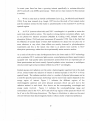
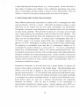
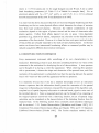
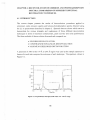
Excited species emit radiation over the entire electromagnetic spectrum but in the study
of hot, ionised matter the radiation of interest is emitted typically in the VUV to X-ray
spectral bands. The radiation emitted is due to a number of physical phenomena and as
a result the specific spectroscopic technology used to record such spectra depends on the
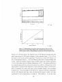
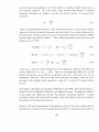
energy region of interest.
Figure
1.1
indicates the different regions
of the
electromagnetic spectrum and some physical processes which can give rise to the
radiation emitted in each band. Also shown are the corresponding wavelength and
energy scales involved.
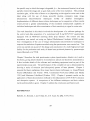
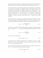
Figure 1.2 indicates the wavelength/energy range and
nomenclature used in the VUV, XUV and soft X-ray regions of the spectrum which will
be of use in the following discussions. The figure is illustrative in nature as the exact
division between these electromagnetic bands is often a matter of personal preference,
3
IO'6
l
10 ' 4
.
I
1 0 10
J
IO"2
.
I
10®
I
1
.
I
10®
I
102
.
I
104
I
I
I
IO2
1
I
ev
1
1
I
Radio- Microwaves
104
.
I
L
I
,
IR
Visible
UV
.
»
Hyperfme structure
Molecular
Molecular Vibrations
Isotopie Sliifts
Rotations
FineStructure
!
Inner Electron
Outer Electron I
Transitions
X-rays
v
Transitions
F ig u r e 1 .1 E n e r g y ra n g e s a n d c o rr e s p o n d in g s p e c tro s c o p ic p h e n o m e n a [B r a n s d e n
an d Jo a ch im 1 9 8 5 ] .
5
4
10
3
10
1
1
1
1
0.1
1
2
10
10
1
1
1
2
I
10
G a m m a RajJfrl
“
e
1
I
I
100 300
S o IH X -ia v s
--------
H ard X - r a y s >
10
I
,
1000 2000 A
V U V ----------- >
^
ELTV
X—
x u v -^ |
F ig u r e 1 .2 T h e w a v elen g th an d p h o to n e n e rg y r a n g e s u sed in th e v a c u u m u ltra v io le t
[S v a n b e r g 1 9 9 1 ].
Studies involving hot ionised matter have been greatly enhanced over the last two
decades due to developments in the technology of high power laser systems. When the
output of a high power (typically Q-switched or mode locked) laser is focused onto a
target in vacuo a short lived (time scales ~ 1 0 '13 - 10'6 sec), high temperature (electron
temperature Te ~ 105 - 108K) and high density (electron density ne ~ 1019 - 1024 cm '3)
plasma is formed. As many of the plasma parameters are to some extent controllable,
the study of laser-produced plasmas (LPP) has greatly extended out understanding of
hot ionised matter. These studies involve analysis of both radiative [e.g., De Michelis
and Mattioli 1984] and particle [e.g., Bonham et al 1988, Kephart et al 1976, Decosk
et al 1984] losses from the expanding plasma.
As well as providing a means of studying hot ionised matter laser plasmas have many
other scientific and technological applications such as x-ray microscopy [Stead et al
1995], high resolution soft x-ray lithography [Frankel et al 1987, Turcu et al 1995], XRay diffraction [He et al 1993], Extended X-ray Absorption Fine Structure (EXAFS)
studies [Malozzi et al 1979, Eason et al 1984, Kubiak et al 1990], pulsed laser
4
deposition dynamics [Murakami et al 1994] and photoabsorption studies of laser
produced plasmas [Costello et al 1991],
1.1 LASER PRODUCED PLASMAS: FORM ATION AND BASIC PHYSICS
As stated above laser plasmas are produced when the focused beam of a laser interacts
with a solid target at irradiances in excess of ~108 W cm ' 2. Laser pulses of such high
power are necessarily of short duration due to the limitations on the average power
available from conventional pulsed lasers and the laser radiation which reaches the target
surface penetrates to only a fraction of a wavelength [Carroll and Kennedy 1981], The
laser radiation penetrating the surface couples strongly to the conduction electrons so
that heating, evaporation and ionisation of the target material occur rapidly. The r.m.s
electric field E in V m"1 is related to the laser flux <]) by the expression
E = 19.4 <j) ^ 2.
So for example if <j) = 1012 W cm" 2 then E = 2 x 109 V m 'l, which is of the order of
0.1% of the field experienced by an electron located one Bohr radius from a hydrogen
nucleus.
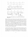
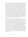
Figure 1.3 shows schematically how a laser plasma is created and what
happens both at the target and within the plasma.
F ig u r e 1 .3 S c h e m a tic d ia g r a m sh o w in g h ow a la s e r -p r o d u c e d p la s m a is fo rm e d
a n d w h a t h a p p e n s a t th e t a r g e t an d w ith in th e p la s m a [F a w c e tt
et al
1 9 6 6 ].
The leading edge of the focused laser pulse vapourises and ionises material from the
surface o f the target and creates a low temperature expanding plasma known as the
priming plasma. This occurs within the first few cycles of the E-field of the laser pulse.
After the priming plasma has been formed absorption of the laser radiation usually
occurs
via inverse Bremsstrahlung. Inverse Bremsstrahlung is a process whereby a
photon is absorbed by an electron-atom/ion system resulting in the electron being raised
from a lower continuum level to a higher one, thereby increasing the kinetic energy of
5
the electron. Inverse Bremsstrahlung is the dominant mechanism in the evolution and
growth o f a LPP. In the early stages of plasma evolution the dominant absorption
process is electron-neutral inverse Bremsstrahlung. When sufficient electrons and ions
are generated the dominant plasma absorption mechanism makes a transition to electronion inverse Bremsstrahlung. The light emitted by a laser plasma results from interactions
between electrons and atomic/ionic species and results in radiation of the following
types occurring:
Line Radiation is due to the spontaneous decay of an excited atom, ion or molecule (in
a bound state) to a lower energy level.
Recombination Radiation (free-bound radiation) occurs when a free electron
recombines with an ion. Since the upper level is continuous the spectrum of the emitted
radiation is continuous, displaying however the characteristic discontinuities at the
wavelengths corresponding to the ionisation energies of bound levels.
Bremsstrahlung (free-free radiation) is emitted, when
electrons
make
transitions
between free energy levels in the field of ions. The resulting spectrum is continuous.
For further details on radiative energy transfer processes within laser plasmas refer to
[Hughes 1975, Dekker 1989],
For plasmas created by a small table top pulsed laser,
typical plasma parameters are as follows :
Laser parameters (specific to D.C.U lab)
Laser type:
Energy (joules):
Pulse lengths (ns):
Nd:YAG
Ruby
1
12
Power densities (W cm ' 2)
1011
Wavelength
1.06 pm
-
1012
1.5
3
25
800
1011 1012
-
694.3 nm
Plasma parameters
Electron Temperatures:
Electron densities:
few eV's - 100 eV
1019c m '3 - 1021c m '3
6
Dye
109 1010
-
340 - 940 nm
In the interest of completeness it is noted that for irradiances > 1013 W cm" 2 several
new physical effects occur within laser plasmas e.g. stimulated Raman back scatter
[Darrow et al 1992], hard X-rays with energies up to 1 MeV [Kmetec et al 1992], high
harmonics of the laser' frequency [Macklin et al 1993], subpicosecond FIR emission
[Hamster et al 1993] and MeV electrons produced by laser wake-field acceleration
[Modena et al 1995], Although these high irradiances are not applicable to this work ,
the physics of plasmas produced by such high irradiances are o f much current interest
and likely to result in many further, novel observations and applications.
1.2 SPECTROSCOPY OF LASER PRODUCED PLASMAS
Laser plasmas have proven to be versatile sources of VUV/XUV line and continuum
radiation and have been used in both emission and absorption spectroscopy. Early
studies o f LPP concentrated on the emission spectra o f multiply ionised species [e.g.,
Fawcett 1984],
The results of these studies combined with ab-initio/sca\ed
multiconfiguration atomic structure calculations have produced a great deal of basic
atomic data along with a greater understanding of the effects of increasing ionisation on
atomic structure. Absorption studies, in particular XUV photoabsorption experiments,
provide important information on inner-shell and double electron excitations and also on
photoionisation continua. The implementation of a photoabsorption experiment has two
basic requirements. The first is the production of an absorbing medium with sufficient
densities o f atomic or ionised species to allow the recording of an absorption spectrum.
The second requirement is to have a smooth, intense and reproducible continuum
(backlighting) radiation source. The radiation from this source being passed through the
absorbing medium.
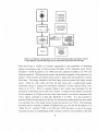
Figure 1.4 below indicates schematically how a photoabsorption experiment is carried
out and
also shows some of the different methods and techniques used in these
experiments.
7
SOURCE
*
SY N C H R O T R O N
V ACUUM SPA RK
4 L A S E R P L A SM A
11
VUV LA SERS
I
N O R M A L IN C ID E N C E
M ONOCHROM ATOR
* G R A Z IN G IN C ID E N C E
XRAY C R Y ST A L
T R A N SIE N T S
STA B LE
SA M PLE
Atoms, Io n s, Excited
A tom s, M o k c u l» an d
Solids.
G A S D IS C H A R G E
VACUUM S P A R K
FL A S H >Y R0LY S1S
ATO M /IC )N BEAM S
H E A T P IP E
W IN D O W L E S S F U R N A C E
L s str
b ttK d >
I tc h n lq a ts
RLD I
Q R (C W )L P P
• LPP
P H O T O G R A P H IC
PM T U B E S
PH O T O D IO D E S
S C IM 1 L L A T O R
DETECTOR
• M CP/PD A
F ig u r e 1 .4 S c h e m a tic r e p r e s e n ta tio n o f a V U V /X U V p h o to a b so rp tio n e x p e rim e n t. Show n
a r e t h e d iffe re n t e x p e rim e n ta l sta g e s an d th e a lte rn a tiv e s a p p r o a c h e s f o r e a c h sta g e .
There have been a number o f inventive approaches to the generation of absorbing
vapours and plasmas such as flash pyrolysis [Tondello 1972] , Resonant Laser Driven
Ionisation - RLDI [Lucatorto et al 1980] and laser plasmas [Costello et al 1991 and
references therein]. Flash pyrolysis systems use powdered samples of the material to be
studied. These samples are placed inside quartz or glass tubes surrounded by a helical
flash lamp. The energy released by the flash lamp produces neutral and singly ionised
atoms
within the tube which can then be used along with a synchronised pulsed
continuum source to measure the absorption spectrum of these species [Roig 1975,
Cantu et al 1977],
RLDI is another effective and widely used technique for the
production of absorbing atomic and ionic columns. A singly ionised column is produced
by the interaction of a high power dye laser beam (tuned to an atomic resonance line)
with a vapour contained in a heat pipe [Mcllrath et a l 1986],
It is also possible to
produce doubly ionised species by the use of a second time synchronised dye laser tuned
to a resonance line of the singly ionised column [Lucatorto et al 1981], This technique
has been used to examine a number of different ions e.g. Ba and N a [Lucatorto et al
1980], Xe, Cs+ and Ba++ [Hill et al 1982 and 1987] and also, as one of its major
successes, provide an understanding of the collapse of the 4 / wave function in Ba with
8
increasing ionisation [Lucatorto et al 1981],
The limitations of the two previous
techniques are that they only provide ionic species with a low degree of ionisation (
singly and doubly charged ions) and in order to study either refractory metal vapours or
ion stages greater than 2+ RLDI is severely limited by restrictions on the experimental
set-ups (e.g. vapour pressures in heat pipes and dye lasers tuned to wavelengths in the
UV). A technique which overcomes these difficulties and which allows the recording of
photoabsorption spectra of multiply ionised species is the Dual Laser Plasma (DLP)
technique in which both the absorbing and backlighting plasmas are produced by the
interaction of high-power laser beams with suitable solid targets.
Before the advent of laser plasma continua, the two most popular XUV light sources
were the BRV vacuum spark and synchrotron radiation. The triggered vacuum spark,
[Ballofet et al 1961], provides continuum radiation in the 80 to 500 A range and has
been used extensively in the production of photoabsorption spectra.
It is a three-
electrode discharge device with continuum emission from a plasma created at the tip of
an electrode. Mehlman and Esteva [1974,1969] using a pair of crossed BRV sparks in
order to generate both the continuum and absorbing plasmas, obtained the VUV and
XUV absorption spectra of Be+ and Mg+ . A problem with using this type of source is
that in order to move to shorter wavelength radiation you must use higher discharge
currents which places limitations on the source repetition rate and electrode lifetimes.
Further this source must be operated in a high vacuum environment.
Synchrotron radiation has also been used also as a continuum radiation source for many
years in photoabsorption studies [see e.g., Wuillemmier 1994],
It has a number of
advantages in that the radiation is intense, free from lines and provides an output whose
energy distribution can be calculated theoretically. Another very important property of
this radiation in for example solid-state studies, is the fact that the radiation has strong
polarisation properties. Using synchrotron radiation in conjunction with an ion beam,
W est and his collaborators obtained absolute photoionisation and photoabsorption crosssections for a number of different ions including K+ [Lyon et al 1986] and Ba+ [Peart et
al 1987], Some of the disadvantages of this source are that it is expensive to operate and
also you must bring your experiments to the machine.
1.2.1 LASER PLASMA CONTINUUM SOURCES
Development of laser plasma continuum sources has increased in recent years due to a
need for convenient small scale sources to act as alternatives to the more conventional
9
devices such as synchrotron and BRV spark. These alternative sources tend to be either
experimentally difficult to use, very expensive, non-portable or have limited spectral
coverage.
[Carroll et al 1978] carried out studies of the continuum emission from a number of rare
earth metals and higher Z materials. In particular, they found that the emission from
elements
samarium (Z=62) to ytterbium (Z=70) was of high intensity
and almost
exclusively continuum in nature apart from a few discrete line features. Further the
continuum radiation was emitted over a broad wavelength range 40 - 2000 Á. These
results stimulated further measurements [Carroll et al 1980,1983] of the time-resolved
and time-integrated emissions from the rare earth metals with a view to establishing
these continuum sources as low cost “table top” alternatives to synchrotron sources for
photoabsorption studies in the VUV and XUV regions. A number of high resolution
studies [Orth et al 1986, Gohil et al 1986] examining the uniformity of these laser
plasma continua have been under taken. These have shown that using a high resolution
grazing incidence spectrograph these spectra are true continua down to a resolution o f 4
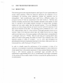
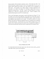
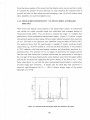
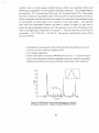
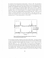
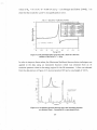
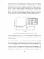
x 10"3 nm. In a contemporaneous experiment [Bridges et al 1986] showed that there
was a progression from mainly line emission for low-Z plasmas to pure continuum
emission for the rare earths (Figure 1.5). The origin of laser-plasma rare earth continua
is discussed in detail by [O’Sullivan 1983] and in the interests of brevity will not be
discussed here.
10
15
20
25
30
35
40
W a v e le n g th (n m )
F ig u r e 1 .5 S p e c t r a sh o w in g th e tra n s itio n fr o m m a in ly lin e em issio n f o r low Z t a r g e t
to p u r e co n tin u u m f o r th e r a r e e a r th s . T h e tra n s itio n f r o m d is c r e te to co n tin u u m
em issio n in th e r a r e e a r th s is a p p a r e n t [B rid g e s
et al
1 9 8 6 ].
Laser plasma continuum sources are advantageous when compared with other
continuum sources for a number of reasons. These are highlighted as follows:
Laser produced plasma continuum light sources
• have good shot to shot reproducibility.
• are insensitive to ambient pressure variations.
• are o f small almost point like spatial extent. This last property is
important for experiments requiring a source of continuum which
provides spatial resolution.
• emit an intense burst of XUV radiation which has very high
instantaneous brightness at least comparable to the flux per pulse
observed from other sources (e.g. synchrotron, BRV spark e.g. [Biijerk
et al 1991, Kuhne et al 1977],
• have pulse widths comparable to the length of the laser pulse.
• are relatively inexpensive and easy to set up.
• exhibit conditions that are controllable/selectable by simple variations
of experimental parameters e.g. laser energy, pulse length, wavelength,
focusing conditions and choice of target material.
• have a wide spectral coverage (30 -> 2000 Á) where the lower bound
of this range is set by the target irradiance
• are free from undesirable line emission.
1.2.2 LASER PLASMA PHOTOABSORPTION EXPERIMENTS AND
DEVELOPMENTS
In the following section a brief discussion of a Dual Laser-Plasma Photoabsorption
(DLPP) technique [Costello et al 1991] in which both the absorbing and backlighting
plasmas are formed by a pair of laser pulses focused onto suitable target materials.
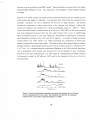
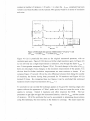
The first two laser plasma experiment carried out was by Carillion et al [1970], In this
experiment they measured the absorption by one aluminium laser-plasma of the flux
emitted by a second Al plasma. These authors found that although the emission was
dominated by discrete line structure there were a small number of narrow wavelength
intervals (of width typically ~ 10 A) which contained predominantly Bremsstrahlung
continuum
emission only.
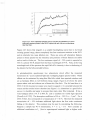
They used this fact to obtain absorption spectra of an
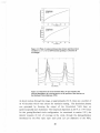
aluminium plasma at a small number of single wavelengths (Figure 1.6).
11
1.6 (a)
F ig u r e 1 .6 (a ) S c h e m a tic d ia g r a m sh o w in g th e e x p e r im e n ta l se t-u p u sed by C a r illio n
et al
1970
to r e c o r d th e a b so rp tio n by a n A l la s e r -p la s m a o f th e flu x e m itte d b y a seco n d A l
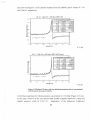
p la sm a , (b ) T r a n s m it ta n c e (T ) s p e c tru m a t 9 8
A sh o w in g t h a t
a t d is ta n c e s ~ 0 .3 m m f r o m th e
t a r g e t s u r f a c e a b so rp tio n is d u e to b o th in v e rs e B r e m s tr a h l u n g a n d p h o to io n isatio n o f
alu m in iu m ions (A l3+) p re s e n t in th e cool o u te r re g io n o f th e re c o m b in in g p la s m a [C a r illio n
al
et
1 9 7 0 ].
Further, it was observed that by varying the time between the generation of the
absorbing and backlighting plasmas (delays used - 1 2 - 2 7
ns) and scanning the
continuum source through the absorbing plasma they could identify different absorption
mechanisms at different stages o f plasma evolution. For short inter-plasma time delays
the absorption decreased smoothly as you moved away from the absorbing plasma core
indicating inverse Bremsstrahlung as the main absorption mechanism. For longer delays
there was a modulation of the total absorption at distances ~ 0.3 mm from the plasma
12
core. This was explained by the fact that as the plasma cooled and expanded there were
ions of low enough charge to allow photoionisation to occur so that absorption of the
backlighting continuum emission could be attributed to both a combination of inverse
Bremsstrahlung and photoionisation.
This experiment showed that laser plasmas could
be used as sources o f continuum for absorption experiments and also provide suitable
absorbing columns o f ions and neutral species. Also by variation of the time delay
between absorbing and backlighting plasmas it possible to obtain time and space
resolved spectra.
A limitation to this experiment was that it could not be used for
photoabsorption studies over a broad wavelength range.
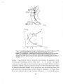
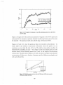
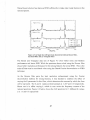
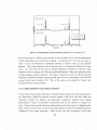
Carroll et al [1977] used the continuum emission from a tungsten laser plasma to
produce the spatially resolved absorption spectrum of singly ionised lithium Li+ The
purpose o f the experiment was to observe the helium like doubly excited states of Li+
and to determine their energies and profile parameters. The absorbing lithium plasma
and backlighting tungsten plasma were generated using a single Q-switched ruby laser
(Fig. 1.7).
F ig u r e 1 .7 D u al L a s e r - P l a s m a (D L P ) e x p e r im e n ta l se t-u p u sed by C a r r o l l an d K e n n e d y [1 9 7 7 ]
to r e c o r d th e p h o to a b so rp tio n s p e c tr a o f L i + . T h e tu n g s te n t a r g e t p ro v id e d a p o in t lik e
s o u rc e o f X U V co n tin u u m ra d ia tio n , w h ich allo w ed th e r e c o r d in g o f s p a tia lly re so lv e d
s p e c tra .
Tungsten was used as a continuum target based on observations made by Ehler et al
[1966] who noticed the predominance of continuum emission in the V-UV spectral
region above 400 A. Carroll and Kennedy also noted in this experiment the importance
of beam focusing conditions in the production of the ionic species to be studied. Also
alignment of the absorbing and continuum sources with respect to one another and the
spectrometer axis was stated as crucial to the success of the experiment.
13
Photographic
plates were used to record the spectra and microdensiometer traces were used in the
determination o f profile parameters q and X [Fano 1961],
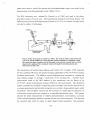
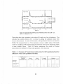
The DLP technique was
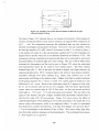
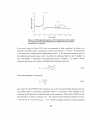
adopted by [Jannitti et a l 1984] and used in the photo
absorption studies of low-Z ions. The experimental procedure and set-up (Figure 1.8)
differed from previous DLP experiments [Carroll et al 1977] in a number of ways which
provided a number of advantages.
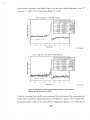
F ig u r e 1 .8 D L P set-u p u sed by [J a n itti
et al
et al
1 9 8 4 ]. T h e se t-u p is s im ila r to th a t o f [ C a r r o ll
1 9 7 7 ] w ith th e a d d itio n o f a X U V d e te c tio n sy s te m c o n sis tin g o f a s c in tilla to r c o a te d
f ib e r -o p tic f a c e p la te c o in c id e n t w ith th e R o w la n d c i r c l e a n d also a to ro id a l m i r r o r , w h ich
im p ro v e s th e c o u p lin g o f th e co n tin u u m ra d ia tio n th ro u g h th e a b s o rb in g p la s m a an d
o n to th e s p e c tr o m e te r slit.
The introduction o f toroidal optics [Rense and Violett 1959, Tondello 1979] improved
the flux coupling efficiency and spectral imaging capabilities of the VUV/XUV grazing
incidence spectrometer. The effective source brightness was increased by viewing the
laser plasma straight on through a small hole in the focusing lens.
Another major
improvement made to the DLP method in this experiment was the fitting of an
VUV/XUV optical multichannel analyser (OMA) to the spectrometer.
This detection
system consisted o f a scintillator coated face plate coincident with the Rowland circle of
a vacuum spectrometer and movable along the curve so that a large spectral region could
be scanned. The scintillator converts the XUV photons to visible light for detection via
a fibre-optic image guide lens coupled to a intensified photodiode array. This system
allowed the direct measurement of relative photoabsorption cross-sections, a process
which with photographic detection systems proved very time consuming. The fact that
the recorded data could be stored in direct digital format permitted
14
deconvolution
(Chapters 3 and 4 discuss this topic further) and other procedures to be applied to the
digitised data to improve the spectral resolution. To improve detector spatial resolution
(and hence spectral resolution) [Cromer et al 1985] fitted a special resolution enhanced
channel electron multiplier array (CEMA - see Chapter 2)
to the front end of the
detector. These CEMA devices consist of an array o f miniature photomultiplier tubes
which are directly sensitive to VUV/XUV photons.
The capabilities o f the DLP technique were further extended by the use of two
temporally synchronised lasers by Carroll and Costello [1986], This approach allowed
increased power densities on targets and variable inter-plasma time delay (At, 250 ns —»
100 p,s).
The system allowed the study of absorption spectra of highly refractory
atomic/ionic species and the production of time resolved absorption spectra of laserproduced plasmas which provides important information about the dynamics of laser
plasmas.
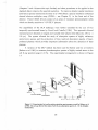
A variation o f the DLP method has been used by Balmer and his co-workers
[Balmer et al 1989] to measure photoabsorption spectra of highly ionised atoms in the
soft X-ray spectral range (1-10 A). The experimental arrangement is shown in Figure
1.9.
F ig u r e 1 .9 E x p e r im e n ta l set-u p f o r p o in t p ro je c tio n s p e c tro s c o p y a s u sed b y B a l m e r
[1 9 8 9 ] . T h is s e t-u p allo w ed th e stu d y o f soft X - r a y a b so rp tio n s p e c t r a (1 - 1 0
ion ised ions.
15
et al
A) o f h igh ly
The absorbing plasma is produced by irradiation with a pulse of 1 ns duration (8-25 J)
focused onto a thin aluminium foil. To produce the backlighting plasma a thin wire ~ 10
mm of either tungsten or Yb coated carbon fiber is irradiated with a short 600 ps pulse
which yields a quasi-point soft x-ray source.
The transmitted X-ray radiation passes
through the absorbing plasma and is dispersed by a crystal spectrometer and recorded on
film. The technique is known as point projection absorption spectroscopy. It provides
quantitative data on the photoionisation cross-sections of highly charged ions.
This
particular method has been used to study bound-bound transitions in hydrogen-like
(A l+12) ancj
helium-like (Al+1*) aluminium ions including satellite as well as resonance
line features. The experiments also provide a quantitative measure of ion ground state
populations which are o f importance in the study of plasma media for e.g., XUV laser
research.
For a more complete review of XUV absorption spectroscopy with laser plasmas and the
different experimental techniques used refer to the article by Costello et al [1991] and
references therein.
1.2.3 EXPERIMENTAL DIFFICULTIES IN VUV/XUV SPECTROSCOPY
In the measurement o f spectra emitted from (and absorbed by) laser-produced plasmas
there are many experimental problems which must be overcome.
The fact that air is
opaque to VUV/XUV radiation means that spectrometers must be evacuated.
Also,
below the LiF 1050A cut-off [Samson 1967], there is a lack of materials which transmit
VUV/XUV radiation. This fact has led to the development of some novel approaches
for confining gases, vapours or plasmas, such as windowless furnaces [Garton et al
1969] and flash pyrolysis [Tondello 1972],
Further it has necessitated the use of
reflective rather than conventional transmissive optics.
The main problem with grazing-incidence spectrometers is the severe astigmatism
entailed (see [Samson 1967] for a discussion of this point). By using a combination of a
toroidal mirror and a grating one can compensate for astigmatic losses [e.g., Rense and
Violett 1959, Tondello 1979], The need to go to grazing incidence at XUV wavelengths
is necessitated by the reflective properties o f gratings and mirrors.
At wavelengths
below 100 nm the reflectivity of materials is < 30 % for nearly all materials at normal
incidence (viewed straight on) and below wavelengths —30 nm this value drops to only
at few percent. This is the reason why normal incidence spectrometers usually operate at
wavelengths longer than 30 nm and also, to minimise the number of reflections, use only
16
a single dispersing and focusing element e.g. a concave grating. On the other hand, at
large angles o f incidence total reflection with a reflectance approaching unity occurs
above a critical angle, and this property is utilised in XUV spectrometers, where the
radiation is incident on the grating at grazing angles of less than a few degrees.
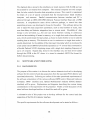
1.3 SPECTROSCOPIC DETECTION SYSTEMS
Many different spectroscopic instruments for studies at XUV wavelengths have been
used (see [Samson 1967] for a review).
Historically the detection systems on these
instruments can be divided into two main types: photographic and photoelectric.
Photographic instruments, using film/plates as the detection media, have the advantage
of image storing capability. They permit the recording of a very large amount of data
with a single exposure; thus permanent records are made for future reference.
This
method o f recording effectively allows the multiplexing of data over a broad spectral
region onto one recording element.
A common type of photographic plate used in
VUV/XUV studies is the Eastman Kodak SWR (short wavelength radiation) type
[Burton et al 1973], Photographic recording also has a number of major disadvantages.
The sensitivity is considerably lower than that of a photoelectric detector; at UV
wavelengths the quantum efficiency is of the order of ~ 1% that o f a photoelectric
detector (e.g., microchannel plate - MCP or VUV sensitive photomultiplier tube). Also
the response is non-linear as a function of the incident energy which makes photometric
calibration a difficult and a time-consuming process. Another problem is the fact the
data stored on plates is not electrical in character so that the measurement of information
recorded must be carried out using a device called a microdensiometer which is a
cumbersome and laborious process.
Photoelectric instruments, on the other hand, have a greater stability of response and
provide a linear output as a function of the incident energy. The photomultiplier tube
(PMT) is one such type of detector. It has a fast response time (better than 5 ns
typically), high sensitivity ( > 103 AAV typical), linear response and wide dynamic range.
However at any one instant it can provide spectral information at one single wavelength
( or averaged over a narrow wavelength interval). In order to record information over a
broad spectral region you must use a scanning monochromator and sequentially
illuminate the detector.
This can lead to problems in the measurement of
absolute/relative intensities for unstable sources. Another problem with a PMT is its
dark current. Even when there is no radiation incident on the detector there is still a
17
background signal present. This problem can be minimised by detector cooling and also
by the suitable choice o f photocathode material.
Over the last 15 years or so array detectors have been developed to act as alternatives
to photographic and single-channel PMT type detectors. They offer the advantages of
electronic read-out of a PMT along with the spatial resolution and multiplexing
characteristics of a photographic plate.
These detectors are solid state devices,
consisting of a large number of light sensitive elements (usually 512 or 1024) closely
arranged in a row.
Each individual element represents one channel of an optical
multichannel analyser (OMA),
in which a count proportional to the intensity of the
incident radiation on the individual element is stored. An OMA is a electro-optical
signal-processing/readout system which when combined with an array detector allows
real-time detection along with image processing capabilities. Array detectors are placed
in the focal plane of the spectrometer and with geometry of 1024 photodiodes, 25 mm
diode separation and 2.5 mm height form effectively a strip of electronic 'photographic'
plate.
To improve the light sensitivity of these devices the array detector is placed
behind an image intensifier device such as a microchannel plate (MCP, see Chapter 2).
This device produces bunches of electrons that are spatially arranged corresponding to
the original radiation spectrum. These electron bunches impinge on a phosphorescent
material. The light thus produced is then transferred to the diode array with the spatial
information retained via fibre-optic coupling device. A more complete description of
such a detector assembly is given in Chapter 2. The above type of diode array detector
was initially developed for plasma impurity analysis in tokamak fusion devices [Fonck et
al 1982, Hodge et al 1984, Schwob et al 1983] but has become widely used in
laboratory spectroscopy. The main benefit of these detectors is their capability to record
simultaneously and digitally acquire whole spectra.
The speed and ease of data
acquisition and processing with these detectors has meant they are attractive alternatives
to photographic and PMT detection systems.
1.4 S PE C T R O SC O PIC IM A G E EN H A N C EM EN T
Spectroscopic imaging systems use either photographic (film, plates) or
photoelectric (PMT’s, Diode Arrays) detection for image sampling and recording and
thus set a limit on the highest spatial frequency which can be recorded.
Further the
optical elements used to produce the images (lenses, mirrors, stops, gratings, etc.)
degrade the quality of the image formed.
The images are therefore instrumentally
smeared with a resultant loss of spatial resolution. It is possible, with a knowledge of
18
the specific way in which the image is degraded, (i.e., the instrument function) to at least
partially restore the image and so gain back some of the lost resolution. The potential
resolution gain, of the order of three or so (depending on the signal to noise ratio in the
data) along with the use of cheap, powerful desktop computers make image
enhancement
(deconvolution)
techniques
worthy
of
detailed
investigation.
Implementation of different deconvolution techniques and a comparison of their results
would provide a greater understanding of the resolution enhancement capability of
individual techniques and allow examination of their sensitivity to signal to noise ratio.
The work described in this thesis involved the development of a software package for
the control and data acquisition of a customised soft X-ray/XUV/VUV spectrometer
equipped with an M CP/self scanning diode array detector. The control and data
acquisition was carried out using an Optical Multichannel Analyser (OMA) system.
Also investigations of the use of image enhancement (deconvolution) techniques to
improve the resolution of spectra recorded using the spectrometer were carried out. This
work was carried out as part of the design and construction of a multi high power laser
facility for the production and study of dense laser-produced plasmas by spectroscopic
means [Kennedy et al 1994],
Chapter 2 describes the total spectrometer system (spectrometer, detector etc.) used in
this thesis, giving details related to its mechanical, optical and electronic characteristics.
It also includes details of the software and interfacing equipment used as part o f the
experimental set-up used. The performance of the complete set up is demonstrated by
showing a series of emission (and absorption) spectra of laser plasmas.
Chapter 3
presents the theory explaining three major deconvolution techniques i.e. Linear/Filtered
Fourier [Michaelian and Friesen 1987], Constrained Non-Linear [Blass and Hasley
1981] and Maximum Likelihood [Frieden 1983] . Chapter 4 presents results on the
application o f these deconvolution methods to the enhancement o f VUV/XUV emission
and absorption spectra.
A comparison of the different techniques and their relative
merits and downfalls is given. Chapter 5 outlines the conclusions and future work.
REFERENCES
Ballofet, G., Romand, J. and Voldar, B., C.R. Acad. Sci. 252, 4139 (1961).
19
Balmer, J., Lewis, C.L.S., Corbett, R.E., Robertson, E., O ’Neill, D., Lamb, M.J.,
Saadat, S., O'Neill, D., Kilkenny, J.D., Back, C.A., Lee, R.W., Phys. Rev. A., 40, 330
(1989).
Bijkerk, F. and Shevel.ko, A.P., SPIE Vol. 1503 Excimer Lasers and Applications III
(1991).
Blass, W.E. and Hasley, G.W., “Deconvolution of Absorption Spectra”, Academic Press
(1981).
Bonham R.W., Quattlebaum J.C, Spectroscopy 3, 42 (1988)
Bransden and Joachim, “The Physics of Atoms and Molecules”, 1985.
Bridges, J.M., Cromer, C.L. and Mcllrath, T.J.,Appl. Opt. 25, 2208 (1986).
Burton, W.M., Hatter, A.T., Ridgely, A., Appl. Opt. 8, 1851 (1973).
Cantu, A.M., Parkinson, W. H , Tondello, G. and Tozzi, G.P., J. Opt. Soc. Amer. 67,
1030(1977).
Carillion, A., Jaegle, P. and Dhez., Phys. Rev. Lett. 25, 140 (1970).
Carroll, P.K. and Costello, J.T., Phys. Rev. Lett. 57, 1581 (1986).
Carroll, P.K. and Kennedy, E.T., Phys. Rev. Lett. 38, 1068 (1977).
Carroll, P.K., and Kennedy, E.T., Contemp. Phys., 22, 61 (1981).
Carroll, P.K., Kennedy, E.T. and O ’Sullivan, G., IEEE. J. Quant Electron. QE-19,1807
(1983).
Carroll, P.K., Kennedy, E.T. and O ’Sullivan, G., Opt. Lett. 2. 72 (1978).
Carroll, P.K., Kennedy, E.T. and O ’Sullivan, G., Appl. Opt. 19, 1454 (1980).
Connerade, J.P., “Giant Resonances in Atoms, Molecules and Solids”, (Edited by J.P
Connerade, J.M., Esteva, and R.C. Karnatak), NATO ASI Series B: Physics Vol. 151, P
3 (1987).
Costello, J.T., Mosnier, J.P., Kennedy, E.T., Carroll, P.K. and O ’Sullivan, G., “X-UV
Absorption Spectroscopy with Laser-Produced Plasmas: A Review”, Phys. Scr. T34,
77 (1991).
Cromer, C.L., Bridges, J.M, Roberts, J.R. and Lucatorto, T.B., Appl. Opt. 24, 2996
(1985).
Darrow, C.B., Coverdale, C., Perry, M.D., Mori, W.B., Clayton, C., Marsh, K , Joshi,
C., Phys. Rev. Lett. 69, 442 (1992).
Decoste, R., Kieffer, J.C., Pascabe, D., Pepin, H , Appl. Phys. Lett., 45, 229 (1984)
Dekker, M., Chapters 1 and 2 and references therein., “Laser-Induced Plasmas and
Applications”, (Edited by Radziemski, L.J. and Cremers, D.A.), (1989).
DeMichelis, C. and Mattioli, M., Rep. Prog. Phys. 47, 1233 (1984).
Eason, R.W, Bradley, D.K., Kilkenny, J.D. and Greaves, G.N., J. Phys. C: Solid State
Phys. 17, 5067 (1984).
20
Ederer, D.L., Phys. Rev. Lett. 13, 760 (1964).
Ehler, A.W. and Weisler, G.L., Appi. Phys. Lett. 8, 89 (1966).
Fano, U., Phys. Rev. 124 1866 (1961).
Fawcett, B.C., J. Opt. Soc. Amer. B l. 195 (1984).
Fawcett, B.C., Gabriel, A.H., Irons. F.E., Peacock, N.J., Saunders, P. A H , Proc. Phys.
Soc., 88 1051 (1966)
Fonck, R.J., Ramsey, A.T. and Yelle, R.V., Appi. Opt., 21, 2115 (1982).
Frankel,
R.D.,
Drumheller,
J.P.,
Kaplan,
A.S.
and
Lubin,
M.J.,
Proc.
of
Microelectronics Seminar Interface 86, Eastman Kodak, p. 82 (1987).
Frieden, B.R, J. Opt. Soc. Amer. 73, 927 (1983).
Garton, W.R.S, Connerade, J.P., Mansfield, M.W.D. and Wheaton, J.E., Appi.Opt. 8,
919, (1969).
Gohil, P., Kaufman, V. and Mcllrath T.J., Appi. Opt. 25, 2039 (1986).
Hamster, H , Sullivann, A., Gordon, S., White, W., Falcone, R.W., Phys. Rev. Lett. 71,
2725, (1993).
He, H , Wark, J.S., RAL Annual Report 93-031, 45 (1993)
Hodge, W.L., Stratton, B.C. and Moos, H.W, Rev. Sci. Instrum. 55, 16 (1984).
Hughes, T.P., Plasmas and Laser Light, Bristol A dam Hilger (1975).
Jaegle, P., J. Physique. Colloq. C9, C9-323, Supplement au n° 12, Tome 58 (1987).
Jannitti, E., Nicolosi, P. and Tondello, G., Opt. Commun. 50. 225 (1984).
Jannitti, E., Nicolosi, P. and Tondello, G., Physica. 124C 139 (1984).
Kephart, J.F., Giovanelli, D.V., Williams, A.H., J. Appi. Phys. 47, 2907 (1976)
Kmetec, J.D., Gordon III, C.L., Macklin, J.J., Lemoff, B E., Brown, G.S., Harris, S.E.,
Phys. Rev. Lett. 68, 1527 (1992).
Kubiak, G.D., Outka, D.A., Rohlfing, C.M., Zeigler, J.M., Windt, D.L., Waskiewicz,
W.K., J. Vac. Sci. Technol. B. 8, 1643 (1990).
Kuhne, M. and Kohl, J., Appi. Opt. 16, 1786 (1977)
Lucatorto, T.B. and Mcllrath, T.J., Appi. Opt. 19, 3948 (1980)
Lucatorto, T.B., Mcllrath, T.J., Sugar, J. and Younger, S.M., Phys. Rev. Lett. 47, 1124
(1981).
Lyon, I.C., Peart, B., Dolder, K. and West, J.B., J. Phys. B19., 4137 (1986).
Macklin, J.J., Kmetec, J.D., Gordon III, C.L., Phys. Rev. Lett. 70, 766 (1993).
Madden, R.P. and Codling, K , Astrophys. J. 141, 364 (1965).
Malozzi, P.J., Schwerzel, R.E., Epstein, H.M. and Campbell, B.E.,“Laser
EXAFS:
Laboratory EXAFS with a nanosecond pulse of laser-produced x-rays”, Science, 206,
353 (1979).
21
Mcllrath, T.J., Sugar, J., Kaufman, V., Cooper, D. and Hill III, W.T., J. Opt. Soc. B3,
398 (1986).
Mehlman, G. and Esteva, J.M., Astrophys. J. 157, 945 (1969).
Mehlman, G., and Esteva, J.M. , Astrophys, J. 188, 191 (1974).
Michaelian, K.H. and Friesen, W.I., Appl. Spec. 42, 1538 (1987).
Modena, A., Najmudin, Z., Dangor, A.E., Clayton, C.E., Marsh, K.A., Joshi, C., Malka,
V., Darrow, C.B., Danson, C., Neely, D., Walsh, F.N., Nature, 3 7 7 , 606 (1995).
Murakami, K., Ohyanagi, T., Miyashita, A., Yoda, O., AIP Conf. Proc. 2 8 8 , 375 (1994).
O ’Sullivan, G„ J. Phys. B 1 6 , 3291 (1983).
Orth, F.B., Ueda, K , Mcllrath, T.J. and Ginter, M.L., Appl. Opt. 25, 2215 (1986).
Peart, B., Lyon, I.C., J. Phys. B. 2 0 673 (1987)
Rense, W.A. and Violett, T., J. Opt. Soc. Am. 4 9 , 139 (1959).
Roig, R.A., and Tondello, G., J. Opt, Soc. Amer. 65 , 829 (1975).
Samson, J.A.R., “Techniques of Vacuum Ultraviolet Spectroscopy”,Wiley & Son (1967)
Svanberg, S., “Atomic and Molecular Spectroscopy”, Springer-Verlag 1991.
Schwob, J.L., Finkenthal, M. and Suckewer, S., Ann. Isr. Phys. Soc. 6, 54 (1983).
Stead, A. D., Cotton, R.A., Goode, J.A., Duckett, J.G., Page, A.M., Ford, T.W., J. XRay Sci & Technol. 5, 52-64, 1995.
Tondello, G., Astrophys. J. 17 2 , 771 (1972).
Tondello, G., Optica Acta, 26, 357 (1979).
Turcu, I.C.E., Reeves, C M ., Stevenson, J.T.M., Ross, A.W.S., Gundlach, A.M.,
Prewett, P., Anastasi, P., Koek, B., Mitchell, P., Lake, P. Microelectronic Engineering
27,
295 (1995)
Wuillemmier, F.J., "New Directions with Third-Generation Soft X-Ray Synchrotron
Radiation Sources", (eds. A.S. Schlachter and F.J. Wuilleumier), Kluwer Academic
Publishers, 47-102(1994)
22
Chapter 2
Experimental
23
CHAPTER 2 : EXPERIMENTAL
2.1
INTRODUCTION
The current chapter describes the main experimental system used to obtain spectral
data presented in the thesis. The main aim is to demonstrate clearly the integration of
grazing incidence spectrometer with array detector, lasers and software resulting in a
complete experimental system for the study of emission and absorption spectroscopy
of laser produced plasmas. The final section of the chapter outlines some of the
measurements done to illustrate the performance of the experimental set-up. These
tests include single shot sensitivity, spectral resolution and noise.
2.2
MULTILASER PLASMA SPECTROMETER SYSTEM
The experimental set-up outlined below was developed to perform photoabsorption
studies of the XUV region of the electromagnetic spectrum. To date it has been
applied to the study o f photoabsorption by plasmas, atoms, ions, excited atoms and
ions, gases and solids [Kennedy et al 1994], The system can also be used to look at
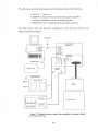
emission spectra. The overall layout of the apparatus used is shown schematically in
Figure 2.1.
F ig u r e 2 .1 S c h e m a tic sh o w in g g e n e ra l f e a tu r e s o f th e D L P e x p e rim e n ta l
set-u p .
24
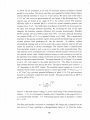
The experimental set-up shown above is based on the DLPP (Dual Laser Plasma
Photoabsorption) technique [Costello et al 1991 and references within] and permits
the measurement of both space and time resolved spectra of laser produced plasmas .
Any photoabsorption experiment has four main elements :
• a source o f continuum emission
• a spectrometer capable of examining the spectral region o f interest
• a sample
• a detector to record the light transmitted through the sample.
The experimental set-up for an emission experiment is very similar except no sample
cell is required and the source of radiation is often a line emission source
(Aluminium Oxide) rather than a continuum source (Tungsten or Tantalum).
2.2.1
DUAL LASER PLASMA EXPERIMENT
A schematic diagram of the dual laser plasma photoabsorption experiment is shown
in Figure 2.1. The capability of this system to perform photoabsorption studies of
neutral, excited and ionic species is achieved through the time synchronisation of two
(or more) pulsed laser systems incorporated in the set-up.
The absorbing column is produced by the ablation of spectroscopically pure targets in
vacuo by either a flash pumped dye laser (~3 J in 1 (is) or by a Q-Switched ruby laser
(~ 1.5 J in 30 ns) focused in either point or line geometry by a spherical or cylindrical
lens respectively. The radiation from the emitting plasma passes through the laser
generated absorbing column and is collected by a toroidal mirror which efficiently
couples the light into a 2.2 metre grazing incidence spectrometer. The XUV light is
dispersed into its constituent wavelengths along the Rowland circle of the
spectrometer. The spectrometer is equipped with a Micro Channel Plate (MCP)
image intensifier, the output of which is proximity focused by means of a fibre optic
face plate, onto a self scanning photodiode array (PDA) detector . After each laser
shot the video signal from the detector is displayed on a digitising oscilloscope
(HP54501 A), thereby permitting the user to monitor variations in continuum intensity
or absorbed signal on a shot to shot basis. A second oscilloscope (HP54502A) is
used to monitor both variations in laser pulse shape/intensity and in optical delay
between laser pulses.
The synchronised video signal from the PDA detector is
digitised and stored in an EG & G Optical Multichannel Analyser (OMA - Model
1461) after each laser shot. If there is jitter in inter laser pulse delay or in relative
intensity from shot to shot any 'rogue' scan can be discarded by the user before
25
accumulation takes place. The accumulated data are then down-loaded into a PC
where the spectra can be stored and/or processed. The operational characteristics of
the key individual components, mechanical, optical and electronic, which together
make up the facility are described in the following sections.
2.2.2
GRAZING INCIDENCE SPECTROMETER
A description o f the spectrometer has been given by Kiernan [1994] and a summary
is included here simply for completeness. A schematic diagram of the spectrometer
is shown in Figure 2.2. When working in the soft x-ray region (2 - 300A) region of
the spectrum it becomes necessary to operate reflection gratings at grazing incidence
due to the poor reflectivity at normal incidence of single optical surfaces at such short
wavelengths [Samson 1967],
The instrument used throughout this work is a Me
Pherson Model 247 M8, 2.2 metre grazing incidence VUV/XUV monochromator
and conforms to a Rowland circle mounting for concave gratings.
The complete
optical system, stainless steel ways, grating chamber, entrance slit assembly and
detector chamber are mounted on a granite base. This has the advantage o f excellent
stability and of providing excellent damping for unwanted vibration. The stainless
steel curved way is fixed to the base plate and then machined to the Rowland circle
radius.
F ig u r e 2 .2 T o p dow n view o f g r a z in g in c id e n c e s p e c tr o m e te r .
The exit slit assembly has been removed and a multichannel detector chamber
installed in its place. This chamber houses an MCP detector, flap isolation valve,
26
pressure gauge ports and is attached by means of an adjustable mount to the carriage
assembly. The carriage assembly utilises a recirculating ball bearing system, assuring
smooth and accurate movement over the entire tracking range.
Correct angular
orientation of the scanning detector assembly to the beam is maintained through all
wavelengths by a straight edge bar.
The bar is built in an upside down "U"
configuration and houses the wavelength drive screw. A manual scanning knob and
mechanical counter assembly is attached to the end of the precision drive screw and
straight edge assembly. Rotation of the knob moves the multichannel detector
assembly along the Rowland circle. The mechanical counter reading is graduated in
inches and indicates the chordal distance from the centre of the grating to the
approximate centre of the detector array. The detector chamber can be moved across
the Rowland circle, i.e., perpendicular to the point of tangent, via an adjustable
translation stage. The adjustment is controlled by means of a micrometer and two
locking screws. Loosening one screw and tightening the other screws moves the
detector across the circle. An isolation valve is located between the detector chamber
and the metal bellows. A support frame has been designed to carry cooling lines to
the detector system which clamps onto the detector chamber. A stainless steel o-ring
sealed bellows connects the detector scanning assembly and the main vacuum
chamber which contains the grating.
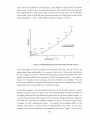
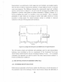
Angle ol Incidence a
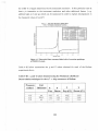
F ig u r e 2 .3 P lo t o f th e v a r ia tio n o f b la z e w a v e le n g th
(A) w ith
a n g le o f
in c id e n c e f o r th e 1 2 0 0 lin es p e r m m g r a tin g u sed in th is s e t o f
e x p e rim e n ts [K ie r n a n 1 9 9 4 ].
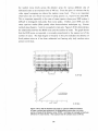
Range o f B ellow s
600 500 -
400 •
300
200
0
4
S
12
16
20
24
28
32
36
Chordal Distance (inches)
F i g u r e 2 .4 P lo t o f th e w a v e le n g th r a n g e s p ossib le w ith a 1 2 0 0 lin es p e r
m m g r a tin g a t an g les o f g r a z in g in c id e n c e fr o m 8 2 ° to 8 8 ° [K ie r n a n
1 9 9 4 ].
27
The main vacuum chamber (housing the grating) is made from stainless steel, sealed
and connected by means of short bellows to a vacuum chamber containing the
entrance slit assembly. Although in a fixed position while in operation, this latter
chamber is easily moved along the curved wave for settings angles of incidence from
82° to 87°, with positive stops in 1/2° increments. All experimental data shown in
this thesis were obtained with the entrance slit maintained on the Rowland circle at
an angle o f incidence o f 84° to the grating normal. The grating used was concave
with a gold coating, ruled at 1200 lines per mm with a blaze angle of 2° 4' ( X biaze =
84.34 A). Figure 2.3 shows the dependence of X biaze on the angle of incidence a. The
grating assembly is kinematically mounted and can be removed/replaced or other
grating assemblies placed in position without further alignment.
The effective
wavelength range of the instrument is determined by the grating being used, the
length of bellows between the scanning detector chamber and the main grating
vacuum chamber and the angle of incidence between the slit and the grating normal.
Figure 2.4 summarises the wavelength ranges possible with the 1200 lines per mm
grating at various angles o f incidence. The wavelength range is inversely proportional
to the number of ruled lines per mm. When substituting a grating not previously
aligned, micrometers provide for fine adjustments on all axes. All motions, except
focus, pivot on a ball bearing at the centre of the grating mount.
The ultimate operating pressure of the spectrometer is determined by the UHY
requirements of the MCP detector. The MCP must be operated at pressures less than
2 x 10'6 mbar.
The vacuum pumping system is connected to the main grating
chamber by means o f a vibration damped bellows terminated with 100mm (inner
diameter) conflat type flanges. There are two types o f vacuum pumps in use. A 240
1/s turbo molecular pump, backed by a two stage rotary, is employed to evacuate the
system starting from atmospheric pressure (having vented and backfilled the
instrument with dry nitrogen). When the pressure has reached approximately lxlO '5
mbar an ion pump is switched on. After the ion pump discharge has stabilised the
turbo pumping system is isolated from the spectrometer via a right angled gate valve
and switched off The ion pump brings the ultimate pressure down in the detector
chamber to less than 2 x 10~7 mbar, well below the minimum operating requirements.
The ion pump is a getter type pump and as such has no need of a backing pump and,
when operated in a UHV environment, it can safely be left running for years without
deterioration in performance. The entire pumping system is supported on a specially
designed rig, the height o f which can be adjusted before connecting to the main
vacuum chamber.
28
2.2.3
MULTICHANNEL PHOTOELECTRIC DETECTION SYSTEM.
For many years integrating detectors in the form of photographic plates were the
basic tools of the spectroscopist. In more recent times, in order to gain the advantages
of direct electronic detection, people have turned increasingly to the use of scanning
instruments with
single channel
outputs
and
electronic
detectors
such
as
photomultiplier tubes or photodiodes. It was long recognised that array or
multichannel detectors would be a powerful and welcome tool if they could be built
with sufficient resolution,
sensitivity and dynamic range. The operational
characteristics of MicroChannel Plates (MCP's) with photodiode or CCD array image
readout meet all o f the above mentioned requirements.
Originally developed as an amplification element for image intensification devices,
MCP's have direct sensitivity to charged particles and energetic photons. Experience
gained in the area o f secondary emission in dynode electron multipliers in the 1960's
and from earlier work on the technique of creating resistive surfaces in lead glass,
together laid the foundation for the development o f this device. The most important
advance came through size reduction techniques achieved by glass fibre drawing
techniques which form the basis of fibre optic device fabrication.
A detailed
description o f the MCP manufacturing process is given by [Wiza 1979],
Ph'mary
R adiation
15 jam
12|im
Vi
-1 kV
Secondary
Em itter
Vo
Vs
+3 to +5 kV
M CP
Phosphor
Vacuum
Seal
Coherent
F ibre optic
R educer
PD A
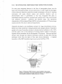
1024 Pixels
F i g u r e 2 .5 D ia g r a m o f M C P d e te c to r sy ste m in s ta lle d in th e g r a z in g
in c id e n c e s p e c tr o m e te r , th e u p p e r h a lf o f th e f ig u r e is a n e x p a n d e d view
o f t h e sig n al in te n sifica tio n re g io n [S ch w o b
29
et al
1 9 8 7 ].
An MCP can be considered as an array of miniature electron multipliers oriented
parallel to one another. The device used here was supplied by Galileo Electro-Optics
and has channel diameters of 12 pm on 15 pm centres. The active area of the matrix
is 12.5 cm2 and covers an approximately 40 mm length of the Rowland circle. The
channel axes are biased at an
angle of 8° to the surface normal. The quantum
efficiency (QE) o f a standard MCP is 10-20% for normal incidence photons with
energies above 15 eV. The OAR (Open Area Ratio) o f the MCP can be increased on
the input side through chemical funnelling. By increasing the area of the open
channels, the detection quantum efficiency will increase proportionally. Standard
MCP's typically will have OAR's greater than 50%; however, chemical funnelling
can produce OAR's of 70 % or greater [Callcott et a l 1988],
This is particularly
important in the grazing incidence regime where geometrical shadowing can prevent
incident photons from penetrating far into the channels.
In addition, surface
photocathode coatings such as Csl (as used with present detector) improve QE and
extend the sensitivity to shorter wavelengths. The channel matrix is manufactured
from lead glass, treated in such a way as to render the walls semiconducting. Thus
each channel can be considered to be a continuous dynode structure which acts as its
own dynode resistor chain. Parallel electrical contact to each channel is provided by
the deposition o f a metallic coating on the front and rear surfaces of the MCP, which
serve as input and output electrodes. The input electrode (Vi in Figure 2.5) is biased
at up to -lk V with respect to the output electrode (Vo). This helps to prevent any
back emitted electrons from leaving the array. The typical electron gain is about 1 x
104, depending on the MCP voltage. The amplified signal emerges as a bunch of
electrons which are then accelerated across a vacuum gap (width = 0.7mm, E neid = 6
x 104 Vcm*1) by a positive potential difference of about 4 kV (Vs) and proximity
focused on a phosphor coated fibre optic bundle. The gain produced by an MCP is
given by [Wiza 1979] :
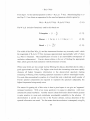
. 4V»a-
G
AV
2 a V,1/2
o /
(2 . 1)
where V is the total channel voltage, V0 is the initial energy of the emitted secondary
electron ~ 1 eV, a is the length to diameter ratio 1/d (typically in the range 40-60), A
is a proportionality constant ~ 0.4. Substituting typical values in Equation 2.1 yields
G ~ 3 x 104.
The fibre optic bundle is mounted on a bakeable UHV flange and is tapered from 40
mm down to 25 mm, resulting in a demagnification factor of 1.6. Thus the visible
30
photon signal produced by the phosphor is readout by a self-scanned 1024 pixel (25
pm x 2.5 mm) PDA (Photo Diode Array - EG & G Model 1453).
2.2.4
PHOTO DIODE ARRAY (PDA) DETECTOR AND COMPUTER
INTERFACE.
Linear silicon photodiode arrays function as photodiodes that are reverse biased and
so they are, in effect, charged capacitors.
W hen light strikes one of these
photodiodes, electrons are released that neutralise holes to discharge the photodiode
capacitance and change the voltage across the diode. During exposure to light, the
voltage on each diode drops proportionally to the light (photons) falling on the diode
during the exposure. During PDA scanning, shift registers and FET switches in the
array package cause the photodiodes to be successively connected to the input of the
detectors amplifier (Figure 2.6).
F ig u r e 2 .6 S im p lified d ia g ra m o f th e P D A d e t e c t o r (M o d el 1 4 5 3 ).
Each successive level defines the integrated light on the addressed pixel. The analog
video signal from the PDA is controlled and read by an EG&G Princeton Applied
Research 1461 Detector interface which forms the heart of the OMA system and is a
desktop size device designed to acquire data from a light detector.
The detector
sends an analog signal through a shielded cable to a detector controller card (EG &
G Model 1462) mounted in a slot of the interface. The controller converts this signal
to digital information that can be used by the interface. In addition, the controller
governs all aspects o f the detector operation including, scanning, triggering and
temperature.
31
The digitised data is stored in the interface's on board memory (32K RAM) and can
be accessed by an external host computer. The external computer not only accepts
data, but also controls the entire data acquisition process. This control is maintained
by means of a set o f special commands that the microprocessor based interface
interprets
and executes.
Parallel communication between interface and PC is
achieved through an IEEE-488 GPIB (General Purpose Interface Bus) and a GPIB
connector. A comprehensive menu driven software package, to control the data
acquisition process, was developed in house by the author. This software allows the
user to adjust the data acquisition parameters, such as total number of scans, inter
scan time-delay and detector integration time in remote mode. Flexibility o f data
storage is also provided; e.g., the user can chose between running in continuous
mode and accumulating all scans in memory, or in single shot mode where after each
scan, which synchronises the laser pulses, a choice is made whether or not to add the
resulting data to memory. This decision to run in continuous or single shot mode is
usually determined by the stability of the inter-laser time delay which is monitored by
a fast optical sensor (BPX65 photodiode operated at a 9 V reverse bias) connected to
a Hewlett Packard 54502A digitising scope with a single shot sampling frequency of
up to 2.5 ns/point. Digital data, stored in the interface unit, are then down loaded
through the GPIB to the PC where it is stored in standard ASCII file format for
further data processing.
2.3
SO FTW A R E AND IN T E R F A C IN G
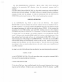
2.3.1
BA CK GRO U N D
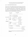
The purpose of this section is to discuss the various elements involved in developing
software for the control o f and data acquisition from the associated PDA detector and
associated electronics. Following an outline of the main operational requirements of
the software a description of the various software (GPIB control files) and hardware
(computer, GPIB
interface card, Optical Multichannel Analyser (OMA) detector
interface) will be given. Explanations and diagrams describing the various timing
considerations in the experiment will be presented. Finally a brief discussion of the
actual software developed and how it should be used will be given.
A substantive aim of this project was to develop software for the control and data
acquisition o f the EG & G detector interface.
The specific requirements for the software development can be stated as follows :
32
• The software had to be intuitive and user friendly so that a first time
user could use the system with relative ease and little tutoring.
• Along with the multichannel spectral experiments carried out,
a time synchronised multi-laser system is used. This
synchronisation was carried out using in house designed
delay generators with an increment of 10 ns and a jitter of ± 5
ns [Lynam et al 1992], The OMA device had to provide a master
trigger pulse which was passed to the delay generators, which in turn
trigger the lasers, in a well defined time sequence. The
software had to ensure that this pulse occurred at the correct
time in the sequence of events during an experiment.
• The last basic requirement o f the software was that it control
and acquire spectral image data from the detector in a simple
and efficient manner with the use of a PC computer and a
detector interface. Spectral images would then be transferred
to the PC computer via the OMA. The software in the PC
would then be required to plot on screen and later to a printer
the spectral image. Facilities such as adding multiple shots,
and averaging files were included in the software.
These are the requirements which were originally stated. Further improvements and
facilities were added to the software during testing of the complete system. These are
discussed later during a more detailed account of the software capabilities.
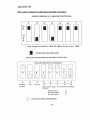
2.3.2
G EN ER A L HARDW ARE / SO FTW A R E D E SC R IPT IO N
The hardware used in the software development and interfacing included the
following :
• Tandon 286 PC-AT computer
• General Purpose Interface Bus (GPIB) card (National
Instruments 488 equivalent)
• EG&G PARC Model 1461 Detector Interface including a
Model 1462 Detector controller
• EG&G PARC Model 1453 Silicon Photodiode Detector
• Hewlett-Packard (HP) 54501A 100 MHz Digitising
Oscilloscope
33
The software used in the development and interfacing included the following :
• Turbo C++ Version 1.0
• GPIB-PC software files and additional programs and files
including installation, test and example programs.
• SPECTRA CALC™ plotting and data analysis software.
The figure below shows the hardware configuration used while the software was
being developed and tested.
F i g u r e 2 .7 S c h e m a tic sh o w in g a ty p ic a l d a ta acq u isitio n s e t-u p u sin g a M o d e l
1 4 6 1 D e te c to r I n te r f a c e .
34
2.3.2.1
TANDON PC
This is an IBM compatible 286 machine with 1 MB o f RAM, 40 MB hardisk,
Advanced MicroDevices math co-processor, VGA monitor and two interface card
slots. This computer was used to program the OMA and acquire data from it. It was
also used as a temporary storage device for the experimental data acquired. Long­
term storage for the data was on 3.5” floppy disks and also on an Apple Macintosh
Ilci computer. The data was transferred from the PC to the Macintosh via a TOPS
network. The TOPS communications card was installed in one o f the PC’s interface
slots, while the GPIB card occupied the other. The data was plotted and analysed on
both the Macintosh and PC.
2.3.2.2
GENERAL PURPOSE INTERFACE BUS (GPIB) AND ITS
ASSOCIATED SOFTWARE
The GPIB is a link, or bus, or interface system, through which interconnected
electronic devices communicate.
This link is used to connect and control
programmable instruments. Typical data transfer rates for the link range from 250
KB to 1 MB per second. These high data transfer rates have led to other applications
such as intercomputer communication and peripheral control. This communication
link is now an industry standard designated as IEEE-488. The IEEE-488 bus is the
most widely used method o f connecting a number o f instruments to the I/O port o f a
computer. Ability to make use o f the bus is a built-in feature on many EG&G PARC
instruments including the Model 1461 Detector Interface.
Communication between devices on the bus is done by passing one o f two types o f
message through the system. The first are known as device-dependent messages and
contain information such as programming instructions, measurement data, machine
status, and data files.
The second type, interface messages, are command type
messages for, say, addressing and unaddressing devices. D evices on the bus can be
listeners, talkers and/or controllers. In this project, the user software and computer
act as talker and listener, the GPIB interface is the controller addressing and
unaddressing talkers and listeners before they send and receive data, while the 1461
Detector Interface is both a listener (receives instructions from computer) and talker
(sends spectral data from its memories to the PC via the GPIB). A talker basically
sends messages to one or more listeners with the controller managing the flow o f
information by sending commands to all the devices.
Using a plug-in interface card and controlling software (discussed below), an IBM
PC or compatible can be converted to a controller in charge o f a wide range o f test
35
equipment. The GPIB interface card used in this project is a PCII-IBM PC interface
card supplied by Integrated Measurements Systems (UK) Ltd..
card which occupies one o f the card slots in the PC.
This is a half-size
Interconection between the
interface and the 1461 interface is made using a standard IEEE-488 cable.
There are a number o f support and utility files which come with the GPIB interface
system which must be installed in order for the interface to operate properly. The
more important files are briefly discussed below :
• GPIB.COM - It is a device handler file that is loaded at system start-up by
the DOS operating system. This file remains resident in memory while the
computer is switched on. It permits all GPIB hardware (talkers, listeners and
controllers) to communicate with one another. It allows you to use different
programming languages, operating systems and computer architecture's.
• IBIC - With the IEEE-488 Bus Interactive Control (IBIC) utility you can
control and communicate with instruments from the keyboard. The IBIC
utility is a simple way to learn the GPIB handler functions and the device
specific commands o f the instrument or to troubleshoot the system.
• IBCONF - A utility program that configures the GPIB interface handler for
GPIB addresses, time-out settings, termination methods, and device-specific
characteristics. The settings entered via this program are then stored in the
file GPIB.COM for use by the interface system. See appendices for the
settings used in this project.
• APPLICATIONS MONITOR - A software utility that performs automatic
error detection and identification. It is a memory resident program which is
useful in debugging sequences o f GPIB calls from within an application
program.
Figure 2.8 displays the important files involved in using a GPIB interface to control a
device. Also shown are the different operating systems and programming languages
which make use o f the handler file GPIB.COM.
36
APPLICATION PROGRAMMING
LANGUAGES
F ig u r e 2 .8 D ia g r a m sh o w in g th e v a rio u s p r o g r a m m in g la n g u a g e s a n d o p e ra tin g
sy stem s w h ich c a n u se th e v a rio u s u tility p r o g r a m s p ro v id e d w ith th e G P I B
s o ftw a re .
The diagram shows that the GPIB is a very flexible method o f communicating with
many devices no matter what the software and hardware used. For this project the
application programming language used was TURBO C, while the operating system
was DOS.
Also the files which the GPIB uses and the application software must be installed
having regard to a particular directory structure.
Details concerning the file
installation are given in the appendices.
2.3.2.3 MODEL 1461 DETECTOR INTERFACE INCLUDING THE MODEL
1462 DETECTOR CONTROLLER
The 1453 PDA array detector described in Chapter 2 is controlled using an electrooptical signal processing/readout system known as a Optical Multichannel Analyser
(OMA).
This system, developed by EG&G PARC laboratories, provides an
extremely fast and powerful computer controlled method for light analysis and
spectroscopy.
The specific type o f OMA system described here is a Model 1461
Detector Interface which houses a range o f cards in vacant slots and allows
connection to one or more PDA detectors (Figure 2.9).
37
F ig u r e 2 .9 M o d e l 1 4 6 1 I n te r f a c e [ E G
& G
1 4 6 1 I n t e r f a c e M a n u a l].
It is a desktop size instrument designed to acquire data from light detectors. The data
are stored in the 1461’s memory and can be read by an external ‘host” computer.
Utilising either user or commercially developed software the external computer not
only accepts data from the 1461, but it is also capable o f controlling the entire data
acquisition process. This is achieved using a Model 1462 Detector Controller. This
is a card, conforming to the virtual memory extended (VME) bus standard, which is
installed in a free slot o f the 1461 interface.
The 1462 controls the spectral data
acquisition by utilising both on and off-board timing circuitry, various amplifiers,
latches and a 12-bit Analog to Digital Converter (ADC). The main functions o f the
controller are to convert the analog signals generated on the detector photodiodes into
digital data (which are then stored in the 1461 interface RAM), provide the timing
required for the controlled scanning o f the detector and also receive and transmit
trigger pulses which can be used to control the experiment. The control is carried out
using a set o f commands specific to the Model 1461, which are sent to it via the
external computer. The interface then interprets the commands and configures the
detector controller to perform the control and data acquisition in the manner specified
by the parameters sent to it by the user. The interface is only used to acquire data
from and control the detector; actual analysis and interpretation o f the data is carried
out by the ‘host” computer and its software. The Model 1461 basically functions as
an interface between the computer and the detector and serves as the power supply
for the detector and the detector controller.
2.3.2.4 MODEL 1461 DETECTOR INTERFACE CONFIGURATION
The following information is just a brief summary o f the interface configuration used
in the experiments relevant to this project. The 1461 interface unit contains mainly
solid state electronics, incorporating VME bus circuitry along with a MOTOROLA™
68000 microprocessor. The timing between the various circuits o f the interface is
38
controlled by a 16 MHz crystal oscillator. The interface has a capacity o f 8 VME
slots. The slots contain the 1461 CPU board and the 1462 detector controller; this
allows for 128 kbytes o f ROM and 32 kbytes o f RAM. This means up to 6 separate
1024 point curves or sets o f readings can be stored in separate memory locations.
The memory is expandable using extra memory boards installed in the vacant slots.
Three interfaces available to the user; serial RS232, a non standard parallel and
IEEE488 GPIB. There are a number o f switch settings which must set in order for
this interface to be addressable. The GPIB dip switches are the ones on the left-hand
side as you look at the CPU board through the rear panel o f the 1461 interface
The
switch settings used are shown in diagrams contained in the appendices.
2.3.2.5 MODEL 1462 DETECTOR CONTROLLER CONFIGURATION
This is an extra VME card which is installed in the 1461 detector interface along with
the 1461 CPU board. The 1462 controller used in these experiments was installed in
slot 8 o f the 1461 interface. The connections between the controller and the rest o f
the experimental set-up are as follows :
• Detector input/output. This is a 25-pin D connector which
provides interfacing to the PDA detector (Model 1453). The
connector holds the timing signals, analog voltages and the
DC power levels that allow detector operation.
• Video Output. This connector transmits the output o f the
1462’s sample-and-hold circuitry. It is used for the real-time
(instantaneous) monitoring o f the signal on the detector
pixels (picture element). This signal is transmitted as a video
signal via a 1 MO connection to a video monitoring device
such as an oscilloscope. It is a useful feature as it allows you
to see what the spectral data looks like without having to first
download and then plot the data.
• Trigger Out (TOUT). The output signal o f this connector is
pixel (28 p.s) wide with rising edge occurring 3 pixels (pixel
no. 1028) after the last analog to digital conversion o f the
detector scan. The availability o f this pulse is software
controlled. The pulse is used to trigger the oscilloscope video
input via a 50 MQ connection and provide a master pulse to
two delay generators used to synchronise the different lasers
used in the experiments.
39
The other connections on the detector controller are explained in the controller user
manual (see references).
2.3.2.6 DETECTOR SCANNING/EXPOSURE TIME CONSIDERATIONS
There are a number o f scanning methods available to the user o f the detector
interface/controller combination. The 1462 controller only allows the use o f a mode
known as the normal scanning mode. During normal scanning, the amount o f charge
on each detector element (pixel) is read by the detector, digitised by the detector
controller, and stored in the 1461 interface.
The basic unit o f time in the 1461 system is called the exposure time. It is the total
time between successive reads o f a detector element i.e. a pixel. It is composed o f
three
basic
elements;
SCAN
TIME,
OVERHEAD
TIME,
VARIABLE
INTEGRATION TIME (VIT). The SCAN TIME is the time required to read/reset
all the detector pixels (1024 pixels for the Model 1453 Detector) as opposed to the
pixel time which is the time required to read/reset one pixel (28 (is).
The
OVERHEAD TIME is immediately after the scan time. It is used by the interface
and controller to make decisions about the next detector scan. For the experimental
configuration used in this project this time is the same for every scan.
The VIT
follows the OVERHEAD TIME and during this period the detector is not being
scanned and the system is basically at rest. There is a trade-off between increased
VIT and dark current build up / saturation. VIT can range from values o f 0 seconds
to larger values which have no practical use. By having a large exposure time you
integrate a greater amount o f flux falling on the detector array, hence you increase the
signal to noise ratio.
Longer exposure times also mean greater build up o f dark
current, which can over a long period o f time saturate the detector. This must be a
consideration when setting the exposure time. For the experiments carried out in this
project, the exposure time is a multiple o f 30 ms. Usually it is set to the minimum
value o f 30 ms, as the laser plasma pulse has duration o f less than 1 (is or so and
hence exposure times greater than the minimum do not improve SNR..
The
following details about exposure times are o f relevance to the 1462 controller used in
conjunction with the Model 1453 detector:
No. of Array Elements
Pixel Time
Base Exposure Time
1024
28 (is
30 ms
The base exposure time consists o f the detector scan time plus the overhead time
explained previously. The exposure time for the 1462 controller is composed o f the
40
base exposure time (30 ms) plus multiples o f this time (delays scans) which make up
the total exposure time.
During these delay scans, which are part o f the VIT, the
array is not read/reset and as a result the flux falling on the pixels is constantly being
integrated. These delay scans are added to the base exposure time if the exposure
time required is greater than 30 ms e.g., exposure time 120 ms means there is a
period o f 4 x 30 ms before the detector pixels are read/reset. The diagrams below
illustrate the various timing and scanning procedures used with the 1461 detector
mterface/1462 controller/1453 detector.
A .
Schematic showing how base exposure time for detector system is defined
|
Base Exposure Time
Overhead Time = 1.328 ms
Scan Time = 1024
x 28 f.is
pixel time
Overhead Time = 30 ms - (1024 x 28 (.is)
B .
Schematic showing trigger pulse available at T R IG OUT connector o f detector controller
TT L Logic 1
28 us wide or 1 pixel wide
TT L Logic 0
N O T E S : This TRIG O UT pulse is software controlled. When data acquisition m ode 4 is used this
pulse appears during the overhead time and before a data acquisition scan takes place.
This is shown below.
C*
Schematic showing where trigger pulse occurs during exposure time when data acquisition
mode 4 is used
N O T E : The rising edge o f the trigger pulse occurs 3 pixels after the last A-to-D conversion
o f the detector scan ie at pixel no. 1028. i.e at (1028 x 28 ^s) o f the 30 ms base
exposure time. This pulse is sent to the delay generators which then fire the lasers.
F i g 2 .1 0 D ia g ra m sh o w in g th e b re a k d o w n o f th e b a s e e x p o s u re tim e o f th e 1 4 6 2
D e te c to r C o n tr o lle r an d w h e re th e T R I G O U T p u lse o c c u r s d u rin g a s c a n .
41
Figure 2.10 shows the situation when the base exposure time is chosen as the
exposure time used during experiments. NOTE : these drawings are not to scale.
The diagrams below show the situation when the exposure time is chosen so that it is
greater than 30 ms. This diagram shows how delay scans are used to increase the
exposure time. This diagram does not include a TRIG OUT pulse before each scan.
M o d el 1 4 6 2 E x p o s u r e T im e , N o rm a l S c a n n in g an d S y n ch ro n is a tio n
DRAWINGS N OT TO SCALE
Exposure Tim e = 120 ms, 1024 elem ents, 28 jxs pixel time
Decisions made
Base exp
time
K-SCAN
SCAN
Overhead Time
Experiment Start
when RU N command
is received.
SCAN
DELAY
SCAN
DELAY
SCAN
DELAY
DELAY
SCAN
SCAN
No data acquisition in this scan
DELAY
SCAN
DELAY
SCAN
^ ----- First data acquisition
in this scan
-----> .
30 ms I 30 ms
30 ms I ------- 120 ms exposure time
exp time I exp time I exp time I
120 ms exposure time
—
—
I
F i g 2 .1 1 M o d el 1 4 6 2 E x p o s u r e T im e
When the detector interface receives the RUN command from the control software it
implements the sequence o f events shown in Figure 2.12. The scan during which the
RUN command is received runs to completion. During the following overhead time
decisions are made about what to do next based on the selected data acquisition mode
The 1461 interface has pre-programmed sets o f commands which perform specific
functions which affect the way it stores and processes the detector data and also the
way it controls the detector using the 1462 detector controller.
The various
commands are detailed and explained in chapters 10 - 17 o f the 1461 interface
instruction manual [see reference list EG & G manuals].
What follows is an
explanation o f the commands which are relevant for this project.
The commands
which control and acquire the data are grouped together in specific programs stored
in the ROM chips o f the 1461. These are known as the data acquisition modes o f the
device.
The data acquisition mode used almost exclusively in the experiments
described here is mode 4.
42
Before a data acquisition mode can be used, the detector interface must have the
relevant parameters sent to it via the host computer.
A listing o f this mode and an
explanation o f how it operates follows:
DP 1
DO I
< ----TOUT
ADD
DOK
IGN
LOOP -<■
LOOP
< —
STOP
\
D ELA Y
LO O P CO N TRO LLED
2
O U TER LO O P PER FO RM S
B Y T H E N U M B E R O F IG N O R E
T H E A C Q U IS T IO N P R O C E S S
SCA N S
A S P E C IF IE D N U M B E R O F
T IM E S
F i g u r e 2 .1 2 D ia g ra m sh o w in g th e listin g f o r th e d a ta acq u isitio n m o d e u sed
b y th e d e te c t o r in te r f a c e d u r in g th e e x p e rim e n ts
The command ‘DPI ’ selects double precision for data storage. There is one set o f T
scans. These are the actual data acquisition scans where the lasers fire due to the
TOUT trigger pulse sent from the detector controller before each scan and the
resulting data, which is imaged onto the array, is read from the detector. After each
scan the data is added into the same memory location previously specified by the
MEM command.
There is a provision for ignoring K scans which allows you to
program a delay between a sequence o f data scans and so allow you to controlthe
frequency o f laser shots.
There are a total o f 17 pre-programmed data acquisition modes available. M ode 4 is
chosen because it is suitable for the experiments carried out for the following
reasons :
• It provides a trigger output pulse (TOUT) which occurs
before the start o f each experiment. This pulse synchronises
events in the experiment from the point o f view o f firing two
lasers at pre-set times using delay generators.
• The data for a number o f laser shots, which is read from the
detector, can be added/accumulated in the one memory
location so that there is a Vn improvement in the signal-to
noise ratio (SNR) over a single scan.
43
• The provision o f ignore scans in the loop means that the duty
cycle o f the laser systems used can accurately controlled.
2.3.2.7
PC OMA SOFTWARE PACKAGE
The menu driven software package developed as part o f this thesis controls the entire
operation o f the 2.2 m spectrometer described above, from triggering the lasers to
fire, to acquiring the resultant spectra from the PDA detector via the OMA control
box. Also post processing o f the data e.g. subtracting spectra , getting the natural
log, plotting etc. was accomplished using the software. The diagram below shows
the main menu and all the sub-functions that can be performed. The software is user
friendly and is activated by typing OMAPROG at the DOS prompt.
Sub - Menus
Main Menu
--------I
GPIB/OMA Initialisation
—Setup
View OM A Configuration
Change OM A Configuration
_Snvc to File
T y p e F r o m D os
Quit OM A Program
_Save Range
—Files
t
_V iew File
— Live
Single Shot Accumulate
—Run
— Single Shot
Run E xperim ent
-Directory
-C hange Directory
-D e lete File
Log Io/Iabs
SOMA
- labs/Io
—Math
- Average/Std Dev
- Add Data
—Plot
Plot D ata File
■c
- Subtract Data
Plot Memory
Integrate Data
■OM A N um bers
—Terminal
■W ipe a Memory
W ipe All Memories
— Exposure Time
— Scans
Scan Delay
Parameters
Memory
DA Memory
— Detector Temp.
F ig u r e 2 .1 3 O M A S o ftw a re F lo w c h a r t sh o w in g M a in M e n u O p tio n s an d
su b -fu n ctio n s.
44
2.4
SPECTROMETER PERFORMANCE
2.4.1
RESOLUTION
The resolving power and reciprocal dispersion (see Figure 2.14) o f a spectrometer are
closely related quantities. While the dispersion determines the separation o f two
wavelengths, the resolving power determines whether this separation can be
distinguished.
Each monochromatic beam itself forms a diffraction pattern, the
principal maxima o f which are represented by the order number m. Between such
maxima, secondary maxima exist whose intensities decrease as the number o f ruled
lines, N, exposed to the incident radiation increases. In practice these secondary
maxima are very much weaker than the principal maxima.
If w e use Rayleigh's
criterion, two lines o f equal intensity will just be resolved when the maximum o f one
falls on the minimum o f the other. The resolving power is defined as X/A X = mN
(for a plane grating), where A A, is the minimum wavelength separation which can be
resolved. Mack et a l [1932] have shown that a slit width W gives rise to an image
width on the focal curve, o f a concave grating in a Rowland mount, corresponding to
a wavelength interval A X =Wd/R, where d is the inter grove spacing and R is the
radius o f curvature o f the grating. Slit widths o f 10 and 20 j.im, combined with a 1200
lines/mm grating o f radius o f curvature = 2.2 m, were used throughout the
photoabsorption/emission experiments described in this thesis which gives rise to an
instrumental line width o f between 0.038 and 0.076 A.
In order to critically assess the performance o f the instrument, in terms o f its
resolution, it was decided to examine the wavelength separation o f some well known
closely spaced lines in the emission spectrum o f a laser produced aluminium plasma.
Using a 1200 lines/mm grating the wavelength
range accessible with the
spectrometer is approximately 80 to 500 A, as determined by the angle o f incidence
on the grating and the available length o f bellows connecting the grating chamber to
movable detector.
45
F ig u r e 2 .1 4 P lo ts o f r e c i p r o c a l d isp ersio n (A /m m ) an d th e o r e tic a l
re so lu tio n (A
X/ X)
f o r a 1 2 0 0 lin e s/m m g r a tin g as a fu n ctio n o f
w a v e le n g th
Pixel Number
F ig u r e 2 .1 5 S p e c tru m o f A 1 V I I em issio n lin es (1 0 p m e n t r a n c e slit)
sh o w in g d e p e n d e n ce o f re s o lv in g p o w e r on th e p ositio n o f th e d e te c to r on
th e R o w la n d C i r c le [K ie r n a n 1 9 9 4 ]
At about midway through this range, at approximately 260 A, there are a number o f
A1 VII doublets which were chosen for resolution testing. The aluminium plasma
was generated by focusing the output o f the Q-switched
YAG
laser on
spectroscopically pure aluminium. The reciprocal dispersion at 260 A is 0.99 A/mm
for this grating/Rowland circle configuration. As mentioned in section 2.2.3, the
detector presents 40 mm o f coverage at the circle, through the demagnification
introduced by the fiber optic taper each pixel (25 pm diameter) o f the PDA,
46
corresponds to a spatial sampling width o f 40 pm on the Rowland circle. Hence, at
260 A each pixel corresponds to a wavelength interval o f ~ 0.04 A. The A1 VII
doublet feature has a wavelength separation o f 0.171 A (~ 4 pixel widths) and should
therefore be a good test o f the resolving power o f the multichannel spectrometer
system.
Early results on emission spectra (the lower most curve in Figure 2.15) in the region
o f this doublet feature (at pixel no. 734) were disappointing. A single broad peak
with very little evidence o f fine structure was observed. Two potential sources of
resolution degradation were examined; firstly the voltage between the exit face o f the
MCP and the phosphor, Vpll, was increased to help reduce the spread o f the emergent
electron bunches. The divergence o f the electron beam is caused by space-charge
repulsion and by the random non axial velocity components o f the electrons as they
exit the channels and reduces as a/^p'1 and hence only a minor improvement was
expected and subsequently observed. Secondly, and more beneficially, the detector
was traversed across the Rowland circle assuming that some degree o f misalignment
and defocusing had occurred. The effect is well illustrated in Figure 2.15 above
where the improvement in resolution is obvious as the detector is moved in 0.01 inch
increments through the point o f best focus.
W a v elen g th (A )
F ig u r e 2 .1 6 S p e c tru m a t o p tim ise d fo c a l p osition on th e R o w la n d c i r c l e
w h e re th e A1 V I I d o u b let a t 2 6 0
A is c le a r ly
reso lv ed .
The spectrum shown in Figure 2.16 was recorded at the optimised detector position
and represents the accumulation o f three laser shots, at an MCP voltage o f -0.930 kV
and phosphor-MCP voltage o f 4.5 kV. On examination o f the doublet feature
47
components, 259.207 and 259.036 one observes that there are 5 pixels separating the
features in comparison to an expected 4 pixels. One cause for a slight loss in
resolution is most probably linked to the size o f the gap between the MCP and the
phosphor.
The dependence o f the diameter (<])) o f the electron-bunch spot on the
phosphor to the MCP-phosphor voltage Vph and gap distance (s) is given to a good
approximation by, (]> = s[Vph]’1/2 [Cromer et a l 1985], A simple calculation with this
formula shows that for a gap s = 0.7mm and Vp^ = 4200 V, (J) « 11 [im.
This is
substantially less than the observed instrument limits o f ~ 4 pixel widths or 100 pm.
However, taking the Nyquist sampling spatial frequency limit o f fsamp > l/2A x, Ax =
pixel width, at least 3 pixel widths are required to avoid aliassing and hence a 4 pixel
limit is quite acceptable.
2.4.2 DETECTOR NOISE PERFORMANCE
A basic understanding o f the origin, behaviour and magnitude o f noise sources in a
spectrometer detection system helps considerably in optimising its signal to noise
ratio (SNR). The PDA detector used here is a parallel imaging detector and the
advantage o f using such a detector is largely determined by its inherent sensitivity and
resolution and by its noise behaviour relative to that o f the system as a whole.
Several sources o f noise are present when signals stored by a PDA are read out.
These have been discussed in detail by a number o f authors [Simpson 1979, Talmi et
al 1980, EG & G Model 1453 Service Manual] and are summarised here.
Before discussing detector noise w e should make brief mention o f the effect o f dark
current zd.
As the temperature o f a PDA is reduced, the number o f thermally
generated electron/hole pairs decreases with a resultant decrease in zd. Dark current id
effectively limits exposure time and hence PD A detectors are normally cooled during
operation.
For data collected in this thesis, an operating temperature o f 5°C was
achieved by means o f a Peltier-effect thermoelectric cooler coupled to the 1453 PDA
camera head.
Additional cooling was provided on this detector by circulating water
through the cooling block at the rear o f the detector housing.
There are a number o f sources o f noise present when the signals stored by the PDA
are read out. The two main components o f this noise 1) Random noise and 2) Fixed
pattern noise. The following sections focus in on the first o f these noise sources as
fixed pattern noise can be removed by subtracting a dark scan from the scan
containing the optical information o f interest (NOTE : this subtraction assumes the
array temperature and readout rate are kept constant and hence this fixed pattern is
constant from scan to scan).
Fixed pattern noise is caused by stray capacitive
48
coupling o f the transients arising from the clock driving signals to the video lines by
external stray capacitances and by diode-to-diode dark charge variations.
2.4.2.1 NOISE SOURCES
Random noise in PDA's is generally due to the following sources :
1. Photon (Shot) noise on the incident light.
2. Shot noise on the dark current.
3. N oise due to the preamplifier
4. The reset noise o f the pixels o f the array ('KTC' noise).
The first noise component is due to the statistical nature o f the arrival o f the photons
at each pixel. This is a natural source o f noise which obey Poisson statistics.
All silicon image detectors are subject to thermally generated dark current and its
associated statistical fluctuations i.e. dark current shot noise. The dark current shot
noise in electrons is given by
(2.2)
where id is the dark current, tl the integration (exposure time) between readouts and
qe the electronic charge. If you take id= 1 pA (dark current at 5°C), t- = 30 ms and qt
= 1.6 x 10‘19 then n6 = 433 which is less than 1 e- / pixel. For ti ~ 1 sec then nd —2
to 3 e- / pixel.
The noise due to the preamplifier is
(2.3)
where k is Boltzmann's constant, B is the bandwidth, T is the absolute temperature,
and k0/gm is the channel resistance o f the input FET and C is the capacitance at the
amplifier input which is composed o f
where Cv is the video line capacitance o f the photodiode array, C
is the
preamplifier input capacitance, and Cs is any stray capacitance due to the amplifier
49
input mode. For B = 10 MHz, kT = 1/40 eV, C = 10 pF then nd w 250 over 1024
pixels.
The pixel reset (or 'KTC') noise is given by
«, = j - /*T C „
(2.4)
where Cp is the pixel (diode) capacitance. The pixel noise is larger than this however
due to the multiple readout switching o f the PDA and the lowest total rest noise
available to an off-chip amplifier is
n, =
/ « X 2 C p + 2Cvc)
(2.5)
He
where Cp is the pixel diode capacitance and Cvc is the video line to clock capacitance.
Applying equation 2.5 to the 1024 pixel S series array used in this thesis, with Cp= 2
pF and Cvc =
1.2 pF yields at 20°C, nr « 1000 and at 5°C, nr « 950.
This noise
contribution tends to be the dominant component on a detected signal.
2.4.2.2 EXPERIMENTAL NOISE DATA.
In order to obtain data regarding noise levels and how they affected the system
performance it was necessary to ensure that the PDA was in a light tight
environment. This was achieved by closing the entrance slit to the spectrometer. The
PDA temperature was set to 5°C to simulate typical experimental conditions and a
number o f different measurements were made. These are summarised and discussed
below.
A series o f measurements were undertaken in order to investigate the relationship
between dark current and dark noise and how these vary with exposure time. This
was done by performing single dark scans o f the array for various exposure times
(30,60,120,240,480,960,1920 ms). A plot o f the pixel value for each exposure time
vs. pixel number is presented in Figure 2.17 (a), while the average dark count vs.
exposure times is shown in Figure 2.17 (b)
50
600
- 30 in s
-
500
G
«400
■
a
0300
60 m s
120 m s
240 m s
480 m s
960 m s
H — 1.92 se c
JaAtM^1UH.W+'lí4^*W,
200
100
=^i!
400
=^=P
600
Pixel N um ber
E xposure T im e (m s)
2.17 (a)
2 17 (b)
F ig u r e 2 .1 7 R e la tio n s h ip b e tw e e n d a r k c o u n t a n d e x p o s u r e tim e on a 1 0 2 4
e le m e n t E G & G silico n P D A (M o d e l 1 4 5 3 ). (a ) P ix e l c o u n ts a c r o s s a r r a y f o r
v a rio u s e x p o s u re tim e s , (b ) R e la tio n s h ip b e tw e e n d a r k c o u n t a n d e x p o s u re tim e .
Figure 2.17 (a) shows that as the exposure time o f the detector increases the dark
pixel count across all 1024 pixels increases. At low exposure times ~ 30 to 120 ms
the count is close to zero and not significant. However, as is clear from Figure 2.17
(b), at an exposure time o f ~ 1 sec one obtains a dark count o f approximately 280
counts.
Given the detector dynamic range o f 2048 counts, this number represents
~14 % o f full scale range at a detector temperature o f 5°C. For spectra which have
low intensity peaks and some continuum present this could be a limiting factor in the
determination o f positions and intensities o f such small peaks. Figure 2.17 (b) shows
that, as expected, the mean dark pixel count increases linearly with increasing
exposure time. From this graph w e see that at low exposure times this relationship,
for the 1453 detector used here, does not hold and the signal is below one least
significant bit volts corresponding to a charge o f ~ 5000 electrons. It was also noted
51
during operation that the detector saturation count is 1786 rather than 2048.
The
observed deviation is likely to be due to (i) the 1453 amplifier gain is too low, (ii) a
negative offset voltage may be sitting on the video signal or (iii) a combination o f
both factors.
The existence o f an offset voltage is strongly supported by the
observation o f an offset in the Figure 2.17 (b) where a signal count o f zero is
obtained for exposure times < 1 2 0 msec. Using 2.17 (b) the intercept is -35 counts.
Adding this to 1786 gives a saturation count o f 1821.
Hence in addition to the
observed offset the gain is only 89 % o f its ideal value.
There is also fixed pattern noise present in each o f the data sets in Figure 2.17 (a).
This effect can be removed by subtracting a second dark scan at the same exposure
time leaving only the true random noise on the difference signal. Figure 2.18 shows
such difference scans (centred at zero counts),
but with an off-set o f 50 counts
added to each data set so that the magnitude and level o f variation can be examined
for each exposure time.
From this plot you can see that the random noise on the
detector array is visibly increasing with exposure time, as expected from equation 2.2
which shows that the dark current shot noise is proportional to the exposure time ty
¡£50
—0 — 3 0 m s
- 0 — 60 ms
—
350
•SB —x|—
-K-
-*e
120 ms
240 ms
480 ms
- A — 9 6 0 ms
100'
- ■ — 1 9 2 se c
-B-
-B-
-Q -,
1 CH—1
I
400
600
■ O ■ I * «O 800
1000
P ixel N um b er
F i g u r e 2 .1 8 R a n d o m n o ise on P D A
The relationship between the mean square value o f the shot noise current znd and the
mean dark current is given by the expression
il = 2 eU Af
52
(2.6)
where Af is the bandwidth o f the detector, e the electronic charge and
the mean
dark current. If the noise in the detection system is truly random shot noise then the
above relationship is valid and the only source o f noise is the shot noise on the dark
current then a plot o f the RMS noise versus the square root o f the dark current should
yield a straight line. This is relationship is plotted in Figure 2.19 below.
1.92 sec
.J Dark Current = ¿d
F ig u r e 2 .1 9 R e la tio n s h ip b etw een th e R M . S n oise an d d a r k c u r r e n t
From this graph w e see for exposure times between 240 and 1920 ms w e have an
approximate linear relationship. At exposure times below 240ms, this relationship
does not appear to be linear. However due to the above mentioned offset in the video
signal one cannot reliably use data below the 240 ms exposure time.
The trend in
Figure 2.19 indicates noise increasing more than linearly with exposure time and
hence noise, sensitive to exposure time and above shot noise is clearly present. Such
additional noise sources could be e.g., thermal in origin.
In the above graphs w e have looked at the noise on the detector array for various
different exposure times for single scans. The following data illustrates the effect o f
averaging scans and how this affects the noise levels on the array readout signals. A
series of measurements were made in which a number o f scans at the same exposure
time (480 ms) were taken for different numbers o f scans. This series o f scans were
averaged for each measurement made.
To examine the averaging effect on the
random noise levels a second series o f measurements were made
at the same
exposure time and subtracted from corresponding first scans. Figure 2.20 (a) shows
53
the random noise levels across the detector array for various different sets of
subtracted scans at an exposure time o f 480 ms. From the plot it is obvious that by
video signal averaging we reduce the random noise level.
This is an important
observation and one which was used in taking spectra i.e., improve the data SNR.
This is important especially in the case o f mean spectra where poor SNR makes it
difficult to distinguish real peaks from noise peaks.
Further, poor SNR can also
cause spurious results (false peaks) when deconvolution techniques e.g., Fourier
methods (see chapters 3 and 4) are applied to data sets. Figure 2.20 (b) demonstrates
the relationship between the RMS noise and the number o f scans. The graph shows
that the RMS noise, as expected, is inversely proportional to the square root o f the
number o f scans. The high degree o f linearity in this plot indicates the absence o f
fixed pattern noise as it has been subtracted out leaving only truly random noise
present on the data.
T.i-JV- yfWw-
T
- 100
r
-8 1
- 64
$0
-4 9
V
.22
-3 6
¡
3§0
-2 5
- 16
- 9
-4
-
400
1
600
Pixel Num ber
2.20 (a)
3,5 - "
¿5
"
o
Z
2*'
1,5 ■■
I::
0,5 + ■
0
0.2
0.4
0.6
0.8
l / V INo. of Scans
I
12
2.20 (b)
F ig u r e 2 .2 0 (a ) P lo t o f a b so lu te n oise c o u n t vs. p ix e l f o r d iffe r e n t n u m b e rs
o f s ca n s a v e r a g e d an d s u b tr a c te d , (b ) R ela tio n sh ip b etw een th e r.m .s n oise
an d no. o f s c a n s o f th e d e t e c to r a r r a y . N O T E : e a c h d a ta s e t in g r a p h (a ) h a s b een
o ff-set b y 1 0 co u n ts c la r it y . T h e e x p o s u re tim e f o r all th e s e s ca n s is 4 8 0 m s.
54
From the above analysis o f the noise from the detector array w e can say that in order
to minimise the amount o f noise observed w e must minimise the exposure time if
possible and also use data subtraction and averaging to get rid o f both random noise
(shot, amplifier, etc.) and fixed pattern noise.
2.4.3 SINGLE SHOT SENSITIVITY .VS. MULTI-SHOT AVERAGED
SPECTRA
With source and detector noise present in the spectrometer system, an experiment
was carried out which recorded single and multi-laser shot averaged spectra o f
Aluminium Oxide (AlO).
This was done to examine the single .vs. multiple shot
performance o f the multichannel spectrometer system. Figure 2.21 shows a single
shot emission spectrum taken using AlO as a target material (exposure time used was
30 ms). The lines in this spectrum were identified using the tables o f Kelly [1987],
The spectrum shows that the spectrometer is capable o f clearly resolving closely
spaced lines e.g., the O VI doublet at 173 A and also that the detector is very sensitive
to XUV radiation with both good spatial resolution and photodiode sensitivity (i.e.
photons/count). The presence o f low ion stages o f aluminium and oxygen and the
fact that very little continuum is present indicate that the spectrometer is looking at
the cool part o f the laser plasma plume, some distance away from the target surface
and that for this particular experiment the power density o f the laser is low. From
these observations w e see that the laser plasma/spectrometer/detector combination
provides single shot sensitivity.
It should also be noted that such sensitivity is
observed right throughout the 25 -> 180 eV photon energy range o f the system
[Kennedy et a l 1994],
Wavelength (A)
F ig u r e 2 .2 1 A lO s p e c tru m sh o w in g th e sin g le sh o t s e n sitiv ity o f sy stem .
55
If the experiment is repeated for multiple accumulated laser shots it is clear from
Figure 2.22 that the resolution is unaffected by multiple shot averaging and is an
indication o f very good mechanical stability o f the spectrometer system. This is most
likely due to the good anti-vibration design o f the system e.g. granite base, damping
legs, etc.
W a v e le n g t h
(A)
F ig u r e 2 .2 2 E f f e c ts o f m u ltip le sh o t a v e r a g in g .
For each spectrum above, w e see that there appears to be a reduction in the intensity
o f the doublet lines with increasing number o f scans averaged. This is most likely
due to the occlusion o f the plasma by the hole/pit generated in the target each time
the laser hits the target.
2.4.4 PHOTOABSORPTION PERFORMANCE
The following section describes the capabilities o f the system for looking at
photoabsorption spectra using a laser plasma continuum light source. To highlight
this potential an experiment was carried out to look at photoabsorption in helium gas,
near the K edge at ~ 500 A corresponding to direct photoionisation and at ~ 206 A
corresponding to double electron excitation. The spectra below were produced by
allowing Helium gas into the laser plasma target chamber. The continuum light is
provided by a laser generated tungsten plasma which acts as the backlighting source
(I0). Figure 2.23 shows a tungsten continuum spectrum covering the full array in the
wavelength range close to 500 A.
56
Pixel
F ig u r e 2 .2 3 X I J V co n tin u u m em ission s p e c t r a ( 1 0 sh o ts a c c u m u la te d ) o f a Y A G
g e n e ra te d tu n g ste n p la s m a in th e 5 0 0
A re g io n
w ith a n d w ith o u t a n alu m in iu m
th in film filte r .
Figure 2.23 shows that tungsten is a suitable backlighting source due to its broad
emitting spectral range, almost completely line free continuum emission in the XUV
and its relatively low mass ablation rate.
There are some self absorption features
present in these spectra but the intensities and positions o f these features are stable
and so tend to divide out. The low continuum signal o f ~ 300 counts is expected as
500 A is almost 400 A distant from the blaze wavelength o f 84 A. Note; at the long
wavelength end o f the spectrum the rapid fall-off in intensity is due to shadowing o f
the detector by the fully extended bellows.
In photoabsorption spectroscopy two phenomena which affect the measured
transmission (I / I0) are scattered light and overlapping higher spectral orders. These
effects can be minimised by using thin film foils which have spectral windows and
act as bandpass filters in well defined energy ranges. Figure 2.23 shows the same
spectra taken with and without one o f these thin film foils. The foil used here is a
2000 A A1 foil mounted on copper wire mesh to support it. It is inserted between the
source and the toroidal mirror chamber (see Figure 2.1). Aluminium is a good foil to
use as it is durable and easier to process than many other filter materials. It has a
wide bandpass (from 170 A to 800 A) and is excellent for visible light rejection
[Powell et a l 1990], The absorption coefficient o f A1 at ~ 500 A is ~ 5 jim"1. For a
2000 A filter, this corresponds to a transmission o f < 40 %. However the measured
transmission o f ~ 55% indicates additional light above the first order continuum
falling on the detector.
This postulate may be seen by considering the following.
Suppose a sample has 40 % transmission, T = I / I0 = 0.4.
N ow consider an
additional contribution to I0 (due to superimposed scattered light or higher order
57
light) is represented by I'. With the A1 filter in place I has I", possibly less than I',
superimposed. Then the transmission is 55% as opposed to 40 % expected.
f= ^ -r
Io+I
(2.7)
Dividing equation 2.7 by I0 w e get
(2 .8)
I/Iq+I /Iq
l+ i/I0
Our expression for T' then becomes
T + l /I 0
T = —— ~ —
1 + 1 I,
.
(2.9)
V }
Substituting our values from above this expression becomes
0.55 = a 4 + ? / —
i+i n .
(2.10)
0.4 + s M
,
(211>
where I"/I0
(S") is the transmitted additional light and I'/I0 (S') is the incident
additional light.
With the A1 filter in place one would expect S' to be substantially greater than S".
Taking say S' = 0.2 w e obtain S" ~ 0.04 as a typical example which confirms this
expectation.
For S' = 0.1 w e obtain S" - 0 . 1
also which would appear to be
unphysical and hence w e conclude that there must be a substantial component o f
additional light on the I0 at ~ 500 A which is significantly reduced on the I.
The general signature o f the above spectra is in good agreement with the
measurements o f Bridges et al [1986] and highlights also the shot to shot
reproducibility o f the backlighting spectrum. This is a key requirement for obtaining
reliable cross-section data.
Measurements made by Kennedy et a l [1994] have
shown that shot to shot variations may be kept below 2% by paying careful attention
to the tungsten target alignment and surface preparation details.
58
F ig u r e 2 .2 4 T u n g ste n C o n tin u u m (I Q) an d H e p h o to a b so rp tio n (I) a t th e 5 0 0 Â
( - 2 5 eV ) ed g e
Figure 2.24 again shows the continuum spectrum o f tungsten in the 500 Â region and
underneath it the absorption spectrum obtained by allowing helium gas to flow into
the chamber. The spectrum clearly shows the K-edge o f helium at 500 Â.
Figures 2.23 and 2.24 show the spectra as they were recorded on the detector. To
obtain relative and absolute cross-section information about the species w e are
examining we must take the ratio o f I to I0. The relative cross-section can then be
determined by calculating Ln (Iq/I) = crnl, where cr is the cross section (cm2), n is the
number density o f the absorbing species (cm-3) and 1 is the length o f the absorbing
column (cm). The plots below (Figures 2.25 and 2.26) show the relative and absolute
cross-sections o f helium as a function o f pressure and for different wavelengths and
with and without foils.
F ig u r e 2 .2 5 R e la tiv e c ro s s -s e c tio n d a ta f o r H e liu m a t d iffe re n t e n e rg ie s
w ith a n d w ith o u t A1 filte rs .
59
F ig u r e 2 .2 6 A b so lu te c ro s s -s e c tio n d a ta f o r H e liu m a t d iffe r e n t e n e rg ie s
w ith an d w ith o u t A1 filte rs .
The data in Figure 2.25 indicates that as w e increase the pressure, while keeping al
remains constant the relative cross section increases, as expected from expression Ln
(Iq^I)
= crnl. For comparison purposes the calculated data are also plotted for
selected wavelengths and pressures o f He gas. W e know 1 and can calculate n from
the ideal gas equation, PV=nRT, where P is pressure in mbar, V is volume in litres, n
is the number o f moles, R is the universal gas constant and T is the temperature in
degrees Kelvin and the values for a are tabulated [Kennedy and Manson 1972], The
discrepancy between calculated and experimental data can be explained by previously
discussed effects o f scattered light and order sorting. The use o f XU V filters helps
eliminate this discrepancy and this can be seen in Figure 2.25 where the calculated
and experimental values for the relative cross sections agree.
The filter reduces
scattered light (for X > 800 A) and also can assist on higher order light reduction by
suppressing light below 180 A. Scattered light is the result o f laser-plasma radiation
specularly reflected from shiny surfaces (e.g., optics, slits, bellows etc.) in the
spectrometer and falling on the detector plane. Higher order light is simply explained
by the grating equation mA, = d (sin a + sin (3). For a given angle o f incidence a and
diffraction (3, mA, = const. Hence at the observation angle [3, A appears in first order
(m =l), A/2 in second order (m=2) etc. For example, with the above experimental
system when we measure light at 350 A first order, w e also get second and third
order light at ~ 175 A and ~ 117 A all at the same pixel number. This can add to the
signal on the detector and give a higher incident (and transmitted) intensity than if
just the first order (350 A) were present.
Figure 2.26 above shows the effect o f
scattered light/higher orders splitting as w e see that according to this graph the cross
section varies with pressure, which is an unphysical effect. In order to understand
this observation consider the following. It is clear from Figure 2.23 and 2.24 that T
< T at all wavelengths in the absence o f the Al filter. This occurs when light other
than first order radiation impinges on the photodetector. The modulated transmission
T ', from equation 2.9, is given by
60
where I" and I' are additional light contributions to I and I0 respectively. At 0.2 mbar
and X = 350 A, T = 0.57 and T' = 0.5. Substituting into expression above gives
which implies
S" = 0.5S' + 0.07
Substituting S' = 0.2 yields S" = 0.03 in expectedly good agreement with the values
obtained in the A1 filter absorption experiment. The further reduction in S" is likely
to the result o f enhanced attenuation o f S" by the He gas.
However the relative
contributions o f scattered light .vs. higher (2nd order) light have not been determined.
Finally an experiment was carried out to look at the photoabsorption spectrum o f
helium in the wavelength range corresponding to double-electron excitation Is2 —>
2snp (~ 200 A) [Madden and Codling 1963, Domke et al 1991], This spectrum is
shown in Figure 2.27 and shows the asymmetric nature o f the resonances which is
due to the interaction between the doubly excited state and the underlying direct
photoionisation continuum producing an interference effect in the cross section. This
series is shown in the energy region ~ 100 A to ~ 215 A in figure 2.27, where up to
the fifth member is clearly visible.
58
60
62
64
66
Photon Energy (eV)
F ig u r e 2 .2 7 P h o to a b s o rp tio n s p e c tru m o f h eliu m g as in th e v ic in ity o f th e
l s 2( 1S ) - > 2 sn p ( XP ) d ou b ly e x c ite d re s o n a n c e s .
An important point to note in the measurement o f the helium photoabsorption cross
section is the insensitivity o f the continuum output o f the backlighting plasma to the
ambient helium pressure. Also, the first member does not display a zero in the crosssection at ~ 60.2 eV.
This is due to the limited resolution o f the system and is
discussed further in Chapter 4.
REFERENCES
Bridges J.M., Cromer C.L. and Mcllrath T., Appl. Opt., Vol. 25, No. 13, (1986).
Carroll, P.K., Kennedy, E.T. , Phys. R ev Lett. 38, 1068 (1977).
Callcot T.A., Ederer D.L. and Arakawa E.T., Nucl. Inst and Meths. in Physics. Res.
A266, North Holland, Amsterdam,578,(1988).
Costello et al, Phys Scr. Review Paper. (1991).
Cromer C.L., Bridges J. M., Roberts J.R. and Lucarto T. B., Appl. Opt., Vol. 24, No.
18, (1985).
Domke, M., Xue, C., Pushmann, A., Mandel, T., Hudson, E., Shirley, D .A., Kaindl,
G., Greene, C.H., Sadeghpour, H R . and Petersen, H , Phys. Rev. Lett. 66 1306
(1991).
EG&G PARC™ Model 1461 Detector Interface Instruction Manual (1990).
EG&G PARC™ Model 1462 Detector Controller and Model 1462/99 14-BIT A/D
Converter Operating and Service Manual (1984).
EG&G PARC™ Model 1461/88 Applications Program Instruction Manual (1989).
Kelly R.L., “Atomic and ionic lines below 2000 angstroms : Hydrogen through
Krypton”, Part I (H-Cr), Part II (Mn-Kr) and Part III (Finding List), J. Physical &
Chem. Ref. Data, Vol 16, supplement No. 1, (1987).
Kiernan, L., PhD. Thesis, Dublin City University (1994).
Kennedy et al, SPIE, 1994.
Kennedy, D.J. and Manson, S.T., Phys. Rev. A. J 1 227 (1972)
Lynam, W.G., Caroll, P.K., Costello, J.T., Evans, D., O'Sullivan, G., J. Phys. B., 25
3963 (1992).
Mack, J.E., Stehn, J.R. and Edlen, B., J. Opt. Soc. Am., 22, 245, (1932).
Madden, R.P. and Codling, K , Phys. Rev. Lett. 10 516 (1963)
McPherson ™, “Instruction Manual for 2.2 Metre Grazing Incidence Vacuum UV
Monchromator”, (1992).
NATIONAL INSTRUMENTS : GPIB-PC User Manual for the IBM Personal
Computer and Compatibles. (April 1988 Ed.) NATIONAL INSTRUMENTS CORP.
Powell F.R., Vedder P.W., Lindblom J.F and Powell S.F., Opt. Eng, Vol 29, No. 6
(1990).
62
Samson J. A., ‘Techniques o f Vacuum Ultraviolet Spectroscopy’’ Wiley & Sons
(1967).
Schwob, J.L., Wouters, A.W., Suckewer, S., Rev. Sci. Instrum. 58 1601 (1987)
Simpson, R.W., Rev. Sci. Inst., 50 730 (1979)
Talmi, Y. and Simpson, R.W., App. Opt. 19 1401 (1980)
Wiza J.L., Nucl. Inst, and Meths, Vol 162, 587, (1979)
63
Chapter 3
Theory of Deconvolution of Instrumental
Broadening Effects in Spectral Data
64
CHAPTER 3 : THEORY OF DECONVOLUTION OF INSTRUMENTAL
BROADENING EFFECTS IN SPECTRAL DATA
3.1 INTRODUCTION
Spreading, blurring, and mixing are qualitative terms used to describe the degrading o f
images due to aberations in imaging optics and the finite spatial resolution o f recording
media.
For example the human eye sometimes 'sees' blurred images due to physical
and/or physiological effect/defects e.g diffraction limit by the pupil/lens, aberations due
to lens shape, retinal damage etc. Like the human eye all other optical instruments are
similarly limited in the fine spatial detail o f an object which they can resolve.
Convolution provides a mathematical framework in which to compute the combined
effect o f each individual contribution to image blurring by complex optical instruments
(e.g a spectrometer) and constitutes a key idea o f the present chapter.
Within spectroscopy there are a number o f forms o f spectral line spreading or blurring
due both to the physical process giving rise to the line and also to the limited resolution
o f the spectrometer/detector combination being used to measure the line profile.
It is
intuitively obvious that little can be done to eliminate or reduce physical broadening
without interfering with the process itself. On the other hand, a knowledge o f how the
spectrometer-detector combination broadens a spectrum line should provide us with a
means o f removing such instrumental broadening. In fact a number o f spectral image
restoration techniques have been developed using this intuitive idea and will be
discussed later in this chapter.
The study o f line profiles in laser-produced plasmas has provided the most important
diagnostic technique o f the last 25 years. Critical to many o f these studies has been the
removal o f additional instrumental broadening.
Hence a brief outline o f a number o f
spectral line broadening mechanisms in laser produced plasmas seems a pertinent
starting point for this chapter.
3.2 PHYSICAL LINE BROADENING EFFECTS
A laser produced plasma consists o f a collection o f electrons and ions undergoing a
random thermal motion within a plasma plume superimposed on the bulk directed
motion o f the plume away from the solid target surface.
In certain laser plasma
experiments it has been observed that, although thermal Doppler broadening is a
65
relatively small contributary factor to observed line widths, ion-motional Doppler effects
result in broad asymmetric line shapes [E.G., Iglesias and Greim
1988], However for
most experiments, due to the potentially high electron and ion densities (particularly in
the plasma core), one must conclude that both electron-impact and quasi-static Stark
broadening (due to ions) are potentially the most significant line broadening
mechanisms.
We discuss briefly in the following subsections the typical relative
contributions o f each o f natural, Doppler and Stark broadening effects.
3.2.1 INHERENT LINE BROADENING EFFECTS
3.2.1.1 NATURAL LINE BROADENING
This is due to the finite lifetime A tf o f any atom in any excited state Ef. As a result o f
this naturally occurring phenomenon, Heisenberg's Uncertainty Principle says that there
will be an uncertainty A E¡ in the value o f Et given by
A Ej A t¡ = h/2n
(3.1)
where h is Planck's constant. For resonance transitions in which the lower level is the
ground state and hence A t -> oo and A E -> 0 w e need only consider the upper state
lifetime. For a line originating from transitions between excited states w e must consider
the total broadening to results from the superpostion o f each A Ej■, A E,
For example consider a resonant transition with A t * 10‘12 sec.
AE =
h/(27rx A t)
= 1.056 x 10-22 J
= 6.6 x lO-4 eV
As A E < 1 meV it is clear that for typical linewidths o f > 100 meV measured in VUV
spectra o f laser produced plasmas that this makes an insignificant contribution.
3.2.1.2 DOPPLER BROADENING
As referred to above this physical broadening effect makes two contributions in the case
o f an expanding laser produced plume.
66
(1)
Due to the random thermal motion o f emitting ions within the plasma
which should result in
a symmetric Gaussian profile e.g
plume
in an A1 plasma with a
temperature o f say 50 eV (~ 6 x 105K) (see Kirkbright 1974)
A X / X = V (2 JcT ln2) / me2
=
V (2 x 1.38 x 10-23 x 6 x 105 X 0 .6 9 3 )/(2 6
=
X
(3.2)
1.67 x 10' 27 x 9 x 1016 )
5 . 5 x l 0 -5
For a typical XUV line say A1 VII 250 A doublet
A A,= 0.013 A
which is small in comparison to the measured width of ~ 0.1 A.
(2)
However ion-motional or 'hydrodynamic' Doppler broadening can in some cases
be many times greater than the above and hence account for the bulk o f the observed
width o f a line [Iglesias and Griem
1988] (in those cases where obviously
Instrumental/Stark broadening cannot be invoked as an explanation). A simple Doppler
shift calculation for an ion expansion velocity o f ~ 105 m/sec yields A X / X ~ 3 x 10-4 and
A X ~ 0 . 1 A at 200 A, which is not too different from typical observed widths (A X / X ~
3 x 10'4).
Although in many cases a combination o f Doppler and Stark broadening
mechanisms must be invoked to explain observed profiles [Nicolosi et a l 1979], some
experiments have been able to isolate regions o f Stark domination close to the target and
o f ion-motional Doppler domination in the expanding plume [Irons et a l 1972], In this
case sophisticated computer models must be used to compute observed line profiles.
3.2.1.3 STARK BROADENING
It is well known that placing an atom in an intense electric field leads to a redistribution
o f the atomic energy levels with a resultant effect on the observed spectrum o f such an
excited atom. In laser produced plasmas intense microfields are present which can result
in such quasi static broadening o f atomic/ionic spectrum lines.
For hydrogen and
hydrogenic ions the full width half maximum (FWHM) for a line at a centre wavelength
A,0 is given by [Befeki - 1976]
67
A h/2= 8.11 x 10'18 x (1-0.7 N d -1/3) x X02 x (n^2 - n22) x ( (Zp) 1/3 / Z e ) x N e 2/3 A
(3.3)
where nj and n2 are the principal quantum numbers o f the upper and lower atomic
states and N e is the electron density given by
N e = No. o f particles in the Debye Sphere
—
1 79 x K)
in12 ^
(eV)]3/‘
- 1.72
| N (m
(3.4)
Ze is the nuclear charge (Ze = 1 for Hydrogen). Zp is the charge on the perturbing ion
and the other symbols have the usual meanings. For example for Hp at 4861 A with N D
= 1016 cm-3 and T = 4eV gives,
A h A » 9.3 A
which is substantially greater than thermal Doppler broadening.
However in a hot
expanding plasma plume the effect o f energetic electrons colliding with ion emitters
must be accounted for.
The details o f such calculations are non-trivial, require a
knowledge o f the atomic structure o f the emitting species and are discussed in some
detail by [Griem 1974],
For the simple case o f Hydrogen Lyman - a , the collisional
half-width is given by
A h A (impact) * 1.62 x 1 0 '17 N e / T 1/2 [13.76 - In (N e 1/2 / T ) ] A
(3.5)
where T = plasma temperature in Kelvin and N e = electron density in cm' 3 . For a
hydrogen plasma with an electron temperature o f 50 eV and density o f 1018 cm-3 , A h «
0.15 A. At long times (|is's) after plasma ignition and / or at significant distances from
the plasma core neutral and singly ionised species are dominant.
In this case Stark
broadening may be computed using Griem [1974]
A h /2 = 2 W ( N e / 1016) + 3.5 A ( N e / 10l6 ) [ i - a N D‘1/3 ] x W ( N e / 1 0 l 6 ) A
(electron impact contribution)
(ion field correction)
(3.6)
68
where a — 0.75 for atoms and 1.2 for singly charged ions and W and A are so called
Stark broadening parameters [cf. Table 13.3 o f Befeki for example data].
For an
aluminium plasma with N e ® 1017 cm' 3 and Te « and 0.7 eV A A- » 14 A is obtained
from the measurement o f the 5593 A line [Knudson et a l 1987] .
It is clear from the above discussion that both ion-motional Doppler boadening and Stark
broadening are the two main physical effects which determine the shape o f emission
lines from laser produced plasmas.
However, the relative contributions o f each
mechanism depend on the region o f plasma viewed and the time o f observation after
plasma ignition.
Further Stark effects depend not only on space / time dependent
parameters (e.g, electron/ion density, temperature etc.) but also on the detailed atomic
parameters o f the line studied. However it is clear that time and space resolved studies
o f line profiles are critically important to the study o f laser plasma physics.
In the next
section w e discuss how instrumental broadening effects on measured profiles may be
reduced using three different deconvolution techniques.
3.3 DECONVOLUTION TECHNIQUES
Every measurement instrument adds something o f its own characteristics to the
measurand. Eliminating at least in part, that extra something that blurs our vision o f the
measurand is the motivation for developing the art o f deconvolution. A true spectrum
can be thought o f as having a comb like appearance.
When observing this spectrum
with a spectrometer, it distorts the shape and dimension o f the spectral lines, and if the
resolution o f the spectrometer is substantially less than the spacing between the spectral
lines it will "wash-out" the comb like appearance o f the true spectrum.
It is intuitively obvious that if one has a detailed knowledge o f how an instrument
distorts a spectrum that this information should permit the restoration o f the spectral
image (not withstanding any limitations imposed by the accuracy o f the algorithm used,
complete loss o f spatial frequency information in selected bands, signal to noise ratio o f
the recorded data etc.). Since a measured spectrum can be thought o f as consisting of
the 'original' spectrum convolved with a 'distorting' function, the art o f spectral image
restoration can be considered as the deconvolution o f the distorting function from the
measured data.
In the following section three commonly used restoration techniques
will be reviewed : 3.3.1 Fourier Deconvolution [Michaelian and Friesen 1987], 3.3.2
Constrained Non-Linear Deconvolution [Blass and Hassley 1981] and 3.3.3 Maximum
Likelihood Deconvolution [Frieden 1983],
69
The Fourier transform method will be
discussed first as it illustrates most clearly many o f the fundamental concepts
underpinning image restoartion via deconvolution.
3.3.1 FOURIER DECONVOLUTION
Before starting the analysis o f the Fourier Deconvolution method it is important to
realise what advantages there are to using the Fourier (or spatial frequency) domain.
The advantages are;
1)
In the way that w e can view electrical signals in either the time and frequency
domain w e can view images in the space or spatial frequency domain. For example, the
diffraction pattern o f a square aperture is simply the Fourier Transform o f the aperture
shape and hence both the shape and its diffraction pattern are interchangable
representatives o f the same entity.
2)
Many processes which degrade experimental data are often manifested largely in
the higher frequency portion o f the Fourier spectrum. The fact that much o f the error
may be localised in a narrow band o f high-frequencies, along with the fact that this band
may be adequately represented by a small number o f discrete spectral components allows
considerable reduction o f the computation burden o f restoration.
3)
Many o f the physical processes that affect optical images and many other types of
experimental data have a simpler mathematical form in Fourier space.
For example
convolution o f two functions in the time/pixel domain is equivalent to multiplication in
the frequency (Fourier) domain.
4)
With the improvements made in the computational efficiency o f the Discrete
Fourier transform for large data sets; Fourier Deconvolution can be significantly faster
than other methods o f computation.
Fourier deconvolution can estimate a more highly resolved spectrum in the following
way. The effect o f Instrumental broadening can be modelled as the convolution o f the
true spectrum O(x) =
{oi ,o2,
,on} with the instrument function M(x) = {mj
,m2, ..... ,mn},
70
(3.7)
I(x) = M(x) ® O(x)
where ® denotes convolution,
(3.8)
I(x) = T m (x - x ' ) 0 O(x)dx'
—oo
where I(x) is the observed image spectrum, 0 (x ) is the true spectrum and M (x) is the
instrument Function (typically a peaked function which falls to zero in both directions
from its maximum).
The convolution integral (3.8), can be greatly simplified if it is expressed in terms o f the
Fourier transform o f the functions involved.
(3.9)
F[I(x)] = F[M(x)] * F[0 (x)]
where F denotes Fourier Transform and where * denotes multiplication.
Since
convolution in the pixel domain is equal to multiplication in the frequency domain this
means (3.9) can be written as
I (ux) = M (ux) * O (ux)
where I (ux), M (ux),
O (ux)
(3.10)
are the Fourier transforms the quantities defined in
equation 3.7. N ow the process o f deconvolution becomes a simple matter o f division.
(3.11)
where F_1[ ] is Inverse Fourier transform and O' (x) is the estimated true spectrum.
In words this means that if the Fourier transform o f the observed spectrum is divided by
the Fourier transform o f the instrument function the result can be inverse transformed to
ideally get back the true spectrum (inverse filtering). In practise things are not so easy;
there are two problems associated with the model.
The first problem is due to noise on the spectrum, which limits the recovery of
resolution.
Since inverse filtering has by its very nature high gain at high spatial
71
frequency the restored spectrum can be significantly contaminated by high levels o f high
spatial frequency noise o f the original measured data set and hence has a poor SNR.
The second problem involves the discrete nature o f the sampled data set. The data set
has in effect been truncated by a rectangular function and an abrupt truncation in the
pixel domain results in generation o f sidelobes (artifacts) in the restored spectrum. This
results from the application o f the infinite continuous Fourier transform to a finite
discretely sampled data set.
These artifacts can be minimised by weighting the
deconvolved function I(x) so that the truncation is not abrupt (a process called
apodisation).
However when this is done there can be
a resultant loss in spatial
resolution.
These problems can be minimised by considering the following. If w e ignore noise for
the moment and apply a filter (apodization function) to the measured data I(x) w e obtain
by Fourier deconvolution o f I(x) yields an estimate o f the true spectrum O(x) given by
, I(ux)W (ux;L )
=
f ' 1[
M ( i)
1
(3 1 2 )
where W (ux;L) is the window function that weights or apodises 1/ M (u) and truncates
the Fourier integral at ux = L. The Finite Impulse Response Operator (FIRO) is defined
as
, W (ux;L)
Rs (x;L> -
(313>
Eq 3.12 can now be expressed as
O'(x) = Rs(x;L) ® I(x)
(3.14)
The expression above enables deconvolution to be visualised in terms o f a filter
operation in which w e restore the spectral image by simple convolution o f the FIRO
Rs (x;L) with the measured data set I(x).
What has not been considered yet in the above analysis is the presence o f noise in the
data. If we include noise, the measured spectrum becomes
I(x) = M(x) ® O(x) + N (x)
72
(3.15)
= I(x ) + N (x )
From Eqn 3.14, the restored spectrum is O'(x) = Rs (x;L) <8>I(x) . Substituting Eqn 3.15
into Eqn 3.14 w e obtain an expression for the resolved spectrum which is given by
O'(x) = Rs (x;L) ® I(x) + Rs (x;L) ® N (x)
(3.16)
The W (x;l) (window functions) used in this thesis are
Triangular = [ 1 - —]
(3-17)
Boxcar = 1 fo r|x | < 1, = Ofor|x] > 1
(3.18)
Bessel = [ 1 - ~ f
1j
(3.19)
The width o f the filter W (ux;L) and the instrument function vary inversely with L while
the magnitude o f Rs (x;L) ® N(x) increases approximately exponentially with L2 when
e.g. M(x) is Gaussian. Thus amplification o f noise is an unavoidable consequence o f
resolution enhancement.
Fourier deconvolution is the art o f finding the appropriate
filter, which gives the best resolution with the minimum o f noise.
When noise levels are low simply inverse filtering the data as described above yields a
good approximation to O(x). For higher noise levels the increasing noise term rapidly
obscures all higher frequency information in the deconvolved spectrum making
truncating or filtering o f the resulting spectrum necessary to achieve meaningful results.
For most data encountered in practice it is found that only a relatively small number o f
Fourier spectral components are required to represent the spectrum adequately; the
higher frequencies being mostly noise.
The reason for getting rid o f this noise is that in pixel space it can give an "apparent"
increased resolution.
With a low noise spectrum it is easier to determine with more
certainty the actual resolution. Another reason is that the Fourier deconvolution process
is quite sensitive to noise and contributes considerable instability to thesolution.
deconvolution is carriedout too far in the Fourier domain, serious
If
distortion o f the
spectral information can result. Too far means that deconvolution is attempted, using Eq
73
3.17, beyond the point at which the spectral information becomes indistinguishable from
the noise.
—
_ . .
System
lra n s te r
Function. T(v)
.
^
V \ .|;..-;
V\
\.
\
\ '
v
Frequency
' - Si gnal L o s t T o N o i s e
F ig u r e 3 .1 R e la tio n s h ip b e tw e e n th e in s tru m e n t fu n ctio n an d n oise in s p a tia l f r e q u e n c y s p a c e .
For this reason it is important to choose an appropriate value o f L (the cut off frequency
o f the filter). Choosing a large value o f L results in a higher resolution but increases the
noise level on the restored data while conversely a smaller value o f L means poorer
resolution but less noise also. A method for determining a value for L for a required
optimal resolution has been devised [Kauppinen et a l 1981] and demonstrates that the
resolution is highly dependent on the data signal-to-noise ratio (SNR) and on the type o f
filter used. Thus the optimum combination depends on the user's aims and criteria.
When the
SNR is sufficiently high, Fourier deconvolution provides a good result.
Moreover, it is easily programmed and also executes quickly. A code written in 'C' has
been developed to investigate the FIRO method o f Fourier Deconvolution.
Some
sample results are presented in Chapter 4.
3.3.2 CONSTRAINED NON-LINEAR DECONVOLUTION
This class o f deconvolution method involves computation in signal space, i.e. directly on
recorded data sets. Van Cittert [1931] is credited with devising the first iterative scheme
for the recovery o f O(x) (the original undistorted spectrum) from I(x) (the recorded
spectrum) directly in signal space. His algorithm may be stated simply as follows :
0 „ = 0 „_1+ { I - 0 „ . 1® M }
74
(3.20)
where w e drop the continuous variable x.
In reality our data set is discrete and x
becomes an array index e.g. (i). We use the subscript 'n' to indicate iteration number
The starting assumption is that
O! = I
(3.21)
i.e. our first guess at the recorded data set is taken to be the measured data set. However
as stated this algorithm has a number o f problems mainly associated with convergence
[Blass and Hasley 1981],
In order to overcome these problems, Jansson [1970] developed a modified Van Cittert
algorithm for which the error factor {I - On ^ ® M} is multiplied by a relaxation (or
weighting) parameter c v The modified algorithm now has the form
0„ = O . J + 0 . ( 1 - OnJ ® M}
(3,22)
As the Van Cittert algorithm involves simple addition, subtraction and convolution it is a
linear process.
On the other hand, Jansson's modification involves multiplication and
hence the often used term that it belongs to the non-linear deconvolution class.
The form o f the relaxation parameter a„ is the key to the success o f the Jansson-VanCittert method.
A number o f functional forms o f otn have been developed and are
summarised below.
In Chapter 4 w e have used the Blass and Hasley form o f the
relaxation function to perform deconvolution using this technique.
•
Jansson [1970] function can be stated as
« . = «„»««[l - 2 |0 „ . , ( x ) - % |]
(3.23)
were a nmax = const and is triangular in shape and generally used with
absorption spectra scaled between 0 and 1.
•
Willson [1973] used a quadratic function
= 4 a„max {On-l(X) “ C°n-1(X) ]2}
75
C3-24*)
= 4 a nmax{O n_1( x ) [ l - O ^ x ) ] }
(3.24b)
designed to overcome potential problems with oscillatory behaviour between
successive iterations.
• Blass and Hasley [1981] have used the function
=
«„m ax { O n - l W t
1
"
O n -l(X) ]
( 3 -2 5 )
which is similar to W illson except for the value o f the exponent 'p' which is
fixed at '1' in the case o f W illson (ignoring the constant factor o f 4).
•
Finally Frieden [1975] has gi ven a relaxation function o f triangular form
which unlike the above three functions may be used with data sets o f arbitrary
minimum and maximum values and is stated as ;
= a nmax[l - 2 (B -A ) '1 | O ^ x ) - % ( A + B) | ]
(3.26)
where A = maximum and B = minimum value o f the data set. For A = 1 and B
= 0 the function reduces to Eqn (3.23) above.
In the code developed as part o f this these the relaxation functions given by equation
3.23 to 3.26 are included. Details on the application o f this code to experimental data
sets are given in chapter 4.
3.3.3 MAXIMUM LIKELIHOOD DECONVOLUTION
Every time w e measure a spectrum w e know that the spectrometer both reveals and
distorts the sample spectrum, that noise is added by the detector, and that furthermore,
each spectrum is just one example o f a statistical process. Therefore the proper question
to ask is : What is the most likely sample behaviour that could have produced the
observed spectrum given the characteristics I know about my instrument ?
Maximum Likelihood techniques answer this question. They give you the m ost probable
76
If the noise is random with a Poisson distribution, then the probability for obtaining a
particular ij is
(o ® m): « e ‘ l
p(ij | o) = ----------------—
(3.29)
Assume that the noise n¡ is uncorrelated with the noise n, , for i,j. Then the likelihood o f
observing the set
,i2,......,i„} is the product o f the probabilities for each o f the ij :
n
I Oj ,o 2, ...... ,o„) = r i p ( i j I o)
i=l
pOi ,i2=
(3.30)
For Poisson noise, this becomes
P(ii
I °i »o2,
. „. i; -(o 0 m)j
^ (o <8>m)j J e
J
,o n) = 1 1 ----------- — j-¡--------------
¡=1
Vi!
(3.31)
The Maximum Likelihood Principle says w e must maximise p, given a set o f constraints.
The two most important constraints are the instrument function and the signal to noise
ratio. This is one advantage with Maximum Likelihood methods that you can include a
priori constraints other than just the instrument function. This allows for a more robust
solution with less probability o f spurious results.
There are many data sets O(x) =
{o x ,o2,......,on}, which, when convolved with the
instrumental function M(x) = {mj ,m2,
,mn} give a result M(x) 0 O (x ) which
conforms to the data within the limits o f the noise. The question is which solution set is
correct ?.
One's intuition says that M(x) ® 0 (x ) should be a smooth curve that fits
somewhere in the middle o f the noisy data set
fluctuations N(x) = {n l,n 2 ,
I(x) = {ii ,i2, ......,in}.
The noise
,nn} should be nearly evenly distributed between positive
and negative values since it is improbable that all the noise fluctuations were negative.
In this instance, intuition and Maximum Likelihood are closely related, because both
deal with probabilities. From the statistics o f the noise, it provides the most probable
solution O(x) = {oi ,o2,...... ,on}.
In order to investigate the usefulness o f this method and compare it with both Fourier
and
Jansson
techniques
a
commercial
78
code
'SSRES'
piggybacked
onto
the
SPECTRACALC™ package is used to implement this method and results presented in
Chapter 4.
REFERENCES
Befeki G ., Principles o f Laser Plasmas (Wiley, N ew York, 1976.)
Blass, W.E. and Hassley, G.W., “Deconvolution o f Absorption Spectra”, Academic
Press (1981).
De Noyer, L.K. and Dodd. I.G., "Maximum Likelihood smoothing o f noisy data.", Am.
Lab. 22 (3), 21-27 (1990).
Frieden B.R., in Picture Processing and D igital Filtering (T. S. Huang, ed.), p. 179.
Springer Verlag, Berlin and N ew York, 1975.
Frieden, B.R, J. Opt. Soc. Amer. 73, 927 (1983).
Griem, H. R. 1974, Spectral Line Broadening by Plasmas. Academic. N ew York.
Iglesias E. J., Greim H.R., Phys. Rev. A. 38, 301 (1988)
Irons F. E. , McWhirter R. W. P. , Peacock N. J. ,
1972 J. Phys. B: Atomic, molec.
Phys. 5 (1975)
Jansson P. A. , Hunt R. H., Plyer E. K. , J. Opt. Soc. Am. 60, 596 (1970).
Jansson P .A ., J. Opt. Soc. Am. 60, 184 (1970).
Kauppinen J.K, Moffat D.J, Cameron D.G, Mantsch H.H, Appl Opt. 20, 1866 (1981)
Kirkbright, G.F.
and Sargent, M. , in Atomic Absorption and Fluorescence
Spectroscopy, Academic Press , 1974.
Knudson J. T., Green W.B. , Sutton D. G. , J Appl. Phys. 61, 4771(1987)
Michaelian, K.H. and Friesen, W.I., Appl. Spec. 42, 1538 (1987).
Nicolosi P. , Tondello G. , Jannitti E . , Phys. Rev. A. 20, 2574(1979).
Van Cittert P .H ., Z. Phys. 69, 298 (1931).
Willson P. D. , Ph. D. Thesis, Michigan State Univ., East Lansing, 1973.
79
Chapter 4
Deconvolution of Emission and
Photoabsorption spectra; Comparison of
different restoration techniques
80
CHAPTER 4 ¡DECONVOLUTION OF EMISSION AND PHOTO ABSORPTION
SPECTRA; COMPARISON OF DIFFERENT SPECTRAL
RESTORATION TECHNIQUES.
4.1 INTRODUCTION
The current chapter presents the results o f deconvolution procedures applied to
aluminium oxide emission spectra and helium photoabsorption spectra obtained using
the 2.2 m spectrometer described in chapter 2. Spectral data are shown which serve to
demonstrate the various strengths and weaknesses o f three different deconvolution
techniques in terms o f resolution enhancement, peak recovery and noise performance.
The three methods o f deconvolution discussed and compared are :
• FOURIER DECONVOLUTION
• CONSTRAINED NON-LINEAR DECONVOLUTION
• MAXIMUM LIKELIHOOD DECONVOLUTION
A spectrum o f AlO in the 170 A to 200 A region was used as the sample spectrum to
deconvolve and inter compare the outcomes o f each technique. The spectrum, shown in
Figure 4.1,
Pixel No.
F ig u r e 4 .1 E x p e r im e n ta l A lO S p e c tru m in t h e 1 7 0 - 2 0 0
81
A ra n g e .
exhibits a pair o f closely spaced doublet features which were examined before and
following the application o f each spectral restoration technique.
The doublet features
are located at ~193 A (pixel position 320) and ~184 A (pixel position 590). These peaks
have been identified using Kelly's tables [1987] and provide good examples o f features
which are partially resolved and which can further be recovered by deconvolution using
an instrumental line shape taken from a spectrum in the same region.
The spectrum
from which the instrumental function was taken is shown in Figure 4.2 and inset is
shown the actual peakshape function used. The spectrum is one o f an AlO plasma in the
same wavelength region as that shown in Figure 4.1. The line used was an A1IV line at
wavelength ~ 161.7 A (2 s2 2p6 —» 2 s2 2p5 3s). The reasons underlying the choice o f this
line are as follows
• the baseline in this spectrum and for this particular line exhibits a low level
o f noise and a low continuum radiation level
• it is a single isolated line
• the full width half at maximum (FWHM) for this line is ~ 3.3 pixels which is
close to this instruments resolution capability and it can therefore reasonably
reliably assumed that the intrinsic linewidth is below that o f the instrument
F i g u r e 4 .2 A lO S p e c tru m f r o m w h ich p e a k s h a p e w a s m e a s u re d
(p e a k s h a p e sh ow n in se t - c o n ta in s 10 p oin ts F W H M 3 .3 p ixels)
82
In an ideal circumstance, the instrument function would represent the true impulse
response o f the spectrometer with no baseline continuum associated with it.
In the
present case, it is necessary that baseline subtraction be performed to generate a
reasonable approximation to a single instrument function profile. It is worth noting that
in Figure 4.1 there is also a peak ( ~ pixel position 540) which was considered for use as
an instrument function but from the observations mentioned below this would not have
been suitable due to the difficulty in performing baseline subtraction and the presence o f
baseline continuum. Before presenting data on each o f the three deconvolution
techniques some observations about peakshapes and the importance o f selecting the
correct one are mentioned below.
These observations are based on deconvolution o f
different experimental spectra, taken with the 2.2m system in Chapter 2, using different
peakshapes and different deconvolution techniques.
• Peakshapes used in deconvolution need to be close to the spectral region
o f interest for the best resolution enhancement. Using instrument functions
from spectral regions far away from the region o f interest can to lead to false
splitting and extra features where there are none. This can be attributed to the
fact that the dispersion o f a spectrometer varies with wavelength, hence the
width o f lines will vary across a spectrum (see Figure 2.13 Chapter 2).
• A lot o f energy and information about an instrument function is contained in
its wings. When a peakshape, isolated from a spectrum is used as an
instrument function, you lose a lot o f information about the peakshape itself
because it is difficult to know where the wings are defined in the presence o f
baseline continuum and system noise Using peakshapes processed like
this can produce artefacts and false peaks in deconvolved spectra in cases
where the peakshape is no longer representative o f the true instrument function.
• peakshapes isolated from spectra and fitted with Gauss-Lorentz lineshapes
produce the best results from the point o f view o f resolution enhancement and
absence o f artefacts and false splitting o f experimental lineshapes. It is known
(and intuitively obvious) that a substantial degree o f both the energy and
information about an instrument function are contained in its wings. It is
known that mixed Gauss-Lorentz or so called Voigt profiles can often provide
best fits to the.instrument function profile wings. Hence Voigt profiles are
used here in those cases where the measured instrument function is curve
fitted and the curve fit subsequently used for spectral restoration.
83
Deconvolution was performed on both single shot and multishot accumulated spectra.
This was done in order to examine the sensitivity o f each method to noise i.e. best and
worst case scenarios. The difference between the experimental single and multishot
spectra is shown below in Figure 4.3. As can be seen the averaging has no affect on the
separation or position o f the peaks, for reasons mentioned in Chapter 2 Section 2.4.3,
but the averaging does result in a smoother or less noisy baseline.
This is important
particularly in cases where you are trying to resolve weak peaks which are in close
proximity to strong peaks. For present purposes interest is confined to improved
resolution in the case o f strong peaks and resonances.
Pixel No.
F i g u r e 4 .3 (a ) S in g le sh o t A lO s p e c t r a , (b ) M u ltis h o t (6 4 ) a v e r a g e d A lO s p e c tr a
The AlO spectra (single and multishot) and peakshape used for each deconvolution
technique were normalised as this is a requirement o f the Constrained Non-Linear
deconvolution method that the data be normalised between 0 and 1.
So to maintain
consistency this approach was used for each o f the other deconvolution methods i.e.
Fourier and Maximum Likelihood.
4.2 DECONVOLUTION OF EMISSION SPECTRA
4.2.1 FOURIER DECONVOLUTION
Before data are presented on the Fourier method, the following is a brief description of
the parameters input to the technique. Fourier deconvolution reduces the halfwidths o f
84
lines by a factor K [Kaupinnen et al 1981], which is in practice limited by the noise in
the measured spectrum.
K is the factor which decides what amount o f spectral
frequency information you smooth or cut-off in the Fourier domain. It is given by the
expression
K
-
4aL
—
(4.1)
where cr is the halfwidth at half max. o f the instrument function, L is the value in Fourier
space above which the spectral frequencies are cut-off and A is a constant determined by
the apodisation functions used as part o f the Finite Impulse Response Operator (FIRO)
Fourier method described in Chapter 3. Three different apodisation functions were used
[Kaupinnen et al 1981]:
x
Triangular = [ 1 - — ]
L
Boxcar =
and
1.772
Au , - ———
i/2
2L
1.207
1 for Ixl < 1, = 0 for Ixl > 1 and Au , = ———
11
11
1/2 2L
Ixl
Bessel = [ 1 - — f
and Au1/2 =
1.904
, N
(4.2)
, N
(4.3)
v
(4.4)
where Au1/2 is the full width half maximum o f the apodisation functions and where w e
get the values for A i.e. Au1/2 = A/2L.
Once w e understand the effect o f K on the
deconvolved spectra, we can choose an optimum value for it. W e know a so w e can
determine a value for L. This is how the Fourier software was written. The K, a and A
are input to the program and it generates a value for L as part o f its deconvolution
process.
With high K values there are significant differences in the SNR o f the restored data as a
result o f the use o f different smoothing or apodisation functions. The higher the value o f
K the greater the differences between the different smoothing functions.
Usually
apodisation defines the instrumental resolution. Hence the higher K, the more critical is
the selection o f the apodisation function.
Figure 4.4 (a) shows deconvolution o f the spectrum in Fig 4.1 but with no filter used (no
apodisation). Compared with the original spectrum there is a significant improvement in
85
the resolution o f the strong peaks at pixel position ~ 340 and ~ 580. The downside to
this simple approach is that by using no filter baseline noise has been amplified with the
possible loss o f information about weak features as they are now indistinguishable from
the noise. The appearance o f non-physical negative peaks is also o f concern. Therefore
we can say that for unfiltered single shot spectra, weak resonances are masked by the
significant noise on the restored spectrum. For comparison purposes Figure 4.4 (b)
shows a sixty four shot averaged spectra deconvolved the same way. There is no real
change in resolution performance o f the strong features in this case but there is a
reduced level o f baseline noise to the point where one can still distinguish the weak
resonances (e.g. O V lines at pixel positions ~ 240 and 280).
Figure 4.4 (a)
•a
&
e — 1 Shot
a—
200
400
6 4 shots
500
P ix e l N o.
F i g u r e 4 .4 A lO F o u r i e r d eco n v o lv ed u n filte re d s p e c t r a (a ) S in g le sh o t
a n d (b ) M u lti sh o t a c c u m u la te d t r a c e s .
W e next discuss the effect o f filtering on the deconvolved spectra. The data in Figure
4.5 (a), (b) and (c) shows the same spectrum deconvolved but with three different types
o f filter or apodisation function applied with a K-value o f 1.6 and c value o f 1.65 for
each filter (Eqn's 4.2 - 4.4).
With the filters we can still see an improvement in
resolution o f the strong peaks but less than that for the unfiltered spectra in Figure 4.4.
On the positive side it is clear that the SNR o f these data is significantly better than that
o f the unfiltered data. Therefore w e can say that the filtering process improved restored
image SNR but at a cost o f reduced resolution. We also note from Figure 4.5 that
86
filtered deconvolution has improved SNR sufficiently to make clear weak features in the
restored spectra.
,— .— .— i— |— ■
— ■
— ■
— -— p
Figure 4.5 (a)
©— Boxcar
a — Bessel
Triangular
F ig u r e 4 .5 (a ) S in g le sh o t A lO s p e c tr u m d eco n v o lv ed w ith (a ) B o x c a r filte r ,
(b ) B e s se l f i lte r a n d (c ) T r ia n g u l a r f ilte r
The Bessel and Triangular data sets o f Figure 4.5 show better noise and baseline
performance and hence SNR. While the spectrum deconvolved using the Boxcar filter
shows better resolution performance for the strong features but worse SNR. This is the
trade-off that must be considered when using the filtered Fourier deconvolution or FIRO
technique.
As the Boxcar filter gave the best resolution enhancement using the Fourier
deconvolution method, for strong features, it was decided to examine the effect o f
varying the K parameter for this filter, which determines the amount by which the lines
will be narrowed. The A and a values are held constant at 1.207 and 1.65 respectively.
Hence one is in effect varying L which in turn varies the frequency content o f the
restored spectrum. Figure 4.6 below shows the AlO spectrum for 3 different K values;
2.4, 1.3 and 0.5 respectively.
87
P ixel No.
F ig u r e 4 .6 (a ) D eco n v o lv ed A IO S p e c tru m w ith B o x c a r f ilt e r a n d (a ) K =
2.4,
(b ) K = 1 .3 an d (c ) K = 0 .5
These plots show that a reduction in the value o f K results in a loss o f resolution. This
indicates that careful selection o f K is critical to getting the optimum results from
Fourier deconvolution. Its value will be based on the apodisation function used and the
SNR o f the measured data i.e., if the spectrum is noisy a smaller value o f K (which
results in smoothing o f the restored spectrum and hence some loss o f resolution) maybe
a more suitable choice.
Table 4-1 below
summarises the results o f Fourier
deconvolution for different K-Values and apodistion / filter functions.
Table 4 - I : Summary of Fourier deconvolution data for AIO experimental data for
different K-Values and apodisation functions.
Boxcar
1.6 / 1.65
B essel
1.6 / 1.65
T riangular
1.6 / 1.65
1. Level of N oise in
restored data
High
Low
Low
2 . R esolution Gain
Good
Poor
P oor
K and H W H M V a lu e ->
Boxcar
K = 1.3
K = 0.5
High
M edium
M edium
Good
P oor
N one
II
Apodisation
Function
Experimental
Observation
88
The appearance o f 'additional' weak features on the spectra in Figure 4.6 on either side
o f the stronger features may be an artefact o f Fourier deconvolution as the instrument
function is comparable with many o f the features w e are trying to deconvolve.
For
broad instrument functions, higher gain at higher spatial frequencies is required to
restore a spectrum which can result in intense noise peaks at high spatial frequency
which look like real peaks.
As we will see, for the Jansson Constrained Non-Linear technique these 'additional' false
peaks do not appear. When the instrument function becomes too broad and the Fourier
method fails, the Jansson technique succeeds by requiring that the intensity o f the
deconvolved bands be positive at all frequencies and the instrument function width be
comparable with the measured lines.
The bottom line with Fourier deconvolution is that to get the best results you must play
around with a number o f different variables which include the value for K i.e., the
selection o f the apodisation function and a knowledge o f the SNR in the data and also
very importantly the instrument function used. The better one’s knowledge o f these
variables, the more confidence one may have in the results obtained from this
deconvolution method.
4.2.2 CONSTRAINED NON-LINEAR DECONVOLUTION
The following data illustrates the application o f the Jansson - Van Cittert Non-Linear
deconvolution technique.
As a reminder, the basic algorithm used is given by the
expression
On = On_! + a n {I - O tl_, ® M}
where the symbols used here have been previously defined in Chapter 3.
presented here makes use o f the relaxation function
(4.5)
The data
a n o f Blass and Hasley [1981]
which is given by the expression
a n = a„m«x {O n-lW D - O n.1( x ) ] } P
(4.6)
The success o f this technique is dependent on the form o f this relaxation function. It is
this parameter that actually makes the technique decidedly non-linear. The data set used
89
to deconvolve is the same as that used for Fourier deconvolution, i.e. A10 spectrum.
Figure 4.7 (a) and (b) show the results o f the application o f this technique to a single
shot and multi-shot accumulated spectra (64 shots) using the following parameters;
number o f iterations = 50, p = 4 and a nmax = 5.
Pixel No.
F i g u r e 4 .7 ( a ) R e s to re d A lO sin g le sh o t s p e c tr u m , (b ) R e s to re d A lO M u ltis h o t
s p e c tru m . W it h th e fo llo w in g p a r a m e t e r s u sed f o r (a ) a n d (b ) n u m b e r o f
ite ra tio n s = 5 0 , p = 4 an d a , , = 5 .
From these data w e see that for both spectra there is very good restoration on the strong
resonances and better SNR performance than the Fourier method. W e also note that for
the multishot spectrum the noise is less as would be expected from observations made in
chapter 2. The resonances around the 340 pixel region appear as a doublet, with one o f
the components broader than the other. From identification o f the lines in this region o f
the spectrum, it is known that there are three O V lines present here 192.906 A, 192.751
A and 192.799 A. The separation o f these later two features is ~ 0.05 A (o f the order o f
one pixel width).
We can see that this method has not resolved these two features
because their separation lies below the Nyquist limit. However this technique does tell
us that there are possibly two features here.
Both spectra in the above case do not appear to have "wall" side features that the Fourier
method gave.
The Jansson method is saying that there are no other features in this
region.
Figure 4.8 shows the sensitivity o f this technique to the relaxation parameter a nmax . In
this case the number o f iterations and the exponent p in equation 4.6 have been kept
90
constant at number o f iterations = 20 and p = 4, where the
a n max parameter has been
varied to see what the effect on the restored AlO spectra would be in terms o f resolution
and noise.
Pixel No.
F ig u r e 4 .8 A IO sin g le sh o t s p e c tru m w ith ite ra tio n s = 2 0 an d p = 4 an d
( “0 ^nm as —
^ nniax — 3 ,2 «IHd
^ iim a x —
Figure 4.8 (a) is practically the same as the original unrestored spectrum, with no
resolution gain seen. Figure 4.8 (b) shows a further slight resolution gain. In Figure 4.8
(c) w e still only see a slight improvement is resolution, even though the factor a nmax is
now 5 times greater compared to Figure 4.8 (a). For each change in the value o f a nmax
there are only slight, if any changes, in the resolution improvement o f the spectra. It is
obvious that for further resolution improvement we must continue to iterate.
If we
compare Figure 4.7 (a) and 4.8 (c), the only difference between them being the number
o f iterations, the former having been processed for 50 iterations and Figure 4.8 (c)
iterated 20 times. By comparing these two figures it can be concluded that continued
iterations result in improved resolution for a nmax = 5.
To conclude we can say that the technique appears to be good for restoring single shot
spectra without the appearance o f "false" peaks and it does not cause the noise in the
spectra to increase.
Indeed it maintains and often improves the SNR.
The key
parameters to get right are again the instrument function, value for a nmax and the number
o f iterations. O f all the problems that can be encountered in attempting deconvolution
using this technique, the most serious is the failure to converge. The main reason for
91
this happening would be the presence o f noise. If the SNR is poor for this technique
then it will diverge and give unphysical results. Caution must be taken not to use too
many iterations and over deconvolute thereby causing the appearance o f "false" peaks.
This technique is similar to the Fourier method in that you must vary different
parameters a number o f times before you get the optimum result.
4.2.3 MAXIMUM LIKELIHOOD DECONVOLUTION.
In this particular case, it was decided to use a commercial package called "SSRES"
which was part o f spectrocopic data analysis package called SPECTRACALC™. The
commercial code was developed using the theory discussed in Chapter 3 for this method.
This technique requires as input the instrument function and an estimate o f the SNR o f
the measured spectral data. The software actually estimates the SNR for the user and
hence one can either use this estimate or input an arbitrary value.
When this method is applied to the AlO spectrum o f Figure 4.3 (a) for two different
SNR ratios w e get the data sets shown in Figure 4.9 (a) ("SSRES" estimates 2% noise in
data) and Figure 4.9 (b) (user estimate o f 10 % noise in data). Figure 4.10 (a) and (b)
are multi shot spectra.
P ix e l N o.
F ig u r e 4 .9 A lO sin g le s p e c tru m w ith n o ise e q u a l to (a ) 2 % a n d (b ) 1 0 %
92
P ix e l No.
F ig u r e 4 .1 0 A lO m u ltish o t s p e c tru m w ith n o ise e q u a l to (a ) 2
%
a n d (b ) 1 0 %
We see that there is a definite improvement in the resolution, but w e see the appearance
o f side wall features as in the Fourier method. An estimate o f 10 % noise was input in
order to force the Maximum Likelihood software to restore noise as real spectral
features. This method permits a test o f the sensitivity o f Maximum Likelihood to data
noise.
As in the case for the Fourier method, Maximum Likelihood ‘restored’ weak
features on the low energy side o f the strong doublet features. Hence the physical reality
o f these features remains uncertain. The data in Figures 4.9 and 4.10 shows that the
Maximum Likelihood method recognises that there are two components in the doublet
centred around pixel position 340.
This is the same as the result for Fourier and
Constrained Non-Linear methods.
4.2.4 COMPARISONS AND CONCLUSIONS
Fourier deconvolution has a tendency to amplify measured data noise and hence Jansson
and Maximum Likelihood generate restored spectra with by far the best SNR and
resolution. Overall the Jansson and Maximum Likelihood methods give similar
performance in terms o f resolution enhancement and do not enhance or amplify the
noise. Fourier does provide resolution enhancement but at the expense o f degrading the
SNR. From a point o f view o f ease o f use and minimal number o f variables Maximum
Likelihood is the better technique.
Both Fourier and the Constrained Non-Linear
93
method have multiple variables which can have multiple values depending on the user so
in this sense these techniques are difficult to use and require a lot o f experience in
choosing the appropriate variable values (different users will get different results for the
same spectral data). The following table below summarises the performance o f each
method in terms o f noise and resolution gain.
Table 4-II : Table comparing the different deconvolution techniques for the
doublet features at pixel positions 340 and 580 in Figure 4.1.
F ourier
Constrained
Non-Linear
Maximum
Likelihood
1. Level of Noise in
restored data
High
Low
Low
2. Resolution Gain
M edium
Good
Good
3. No. of Input
parameters
M ultiple
M ultiple
2
High
Low
M edium
Experimental
Observation
4. Level of
spurious features
after restoration
4.3 DECONVOLUTION OF PHOTOABSORPTION SPECTRA
4.3.1 INTRODUCTION
The well known extreme-UV (XUV) absorption spectrum o f helium was used to test
both the photoabsorption capability o f the system and the potential use o f deconvolution
methods to determine restored resonance profiles.
The Maximum Likelihood method was chosen as the deconvolution technique to
examine photoabsorption spectra and deconvolution because it accounted for the SNR
o f the data and had comparable resolution to the Jansson method and didn’t require any
arbitrary filter or window functions as used in FIRO and Non-Linear methods. Hence
one can conclude that the objectives o f the Maximum Likelihood (best estimate) makes
it the optimum candidate for the present exercise.
94
The usefulness o f the deconvolution process , as applied to photoabsorption spectra,
could be measured in terms o f the determination o f resonance parameters o f features
present in the spectrum o f Helium. W e know that the photoabsorption cross section for a
certain element represents a measure o f the probability that a photon will be absorbed as
a function o f the photon energy. For helium these cross sections are larger at certain
energies which result in resonances which have a characteristic shape known as a FanoBeutler profile (see Fano [1961]).
Normally
in photoionisation
/
absorption- experiments
one would
expect the
photoionisation cross section to decrease monotonically as one moves toward higher
photon energy away from the ionisation threshold. In the case o f helium, asymmetric
resonances in the photoabsorption cross section were observed by Madden and Codling
[1965] some 30 years ago.
The origin o f these resonances as atomic interference
phenomena had been discussed in some detail some years previously by Fano [1961],
Briefly for an incident photon energy o f ~ 60.15 eV two outcomes are possible :
• direct single ionisation resulting in a He+ ion and a free electron.
• one photon two electron excitation Is2 —> 2s 2p
The doubly excited (Is2 - » 2s 2p) state is clearly unstable and undergoes a process by
which one o f the electrons is "shaken o f f - so called autoionisation.
Clearly we have a situation in which the final state i.e. He+ and a free electron maybe
reached by two competing pathways, each with its own probability amplitude which are
themselves photon energy dependent and hence the net result is an atomic interference
phenomenon i.e. asymmetric Fano shape.
4.3.2 DECONVOLUTION OF HELIUM PHOTOABSORPTION SPECTRA
Figure 4.11 shows an experimental helium photoabsorption spectrum obtained with the
spectrometer described in chapter 2. The helium pressure was 0.28mbar and no foil was
used. You can see clearly from this spectrum the Is2 —>• 2s np (n = 2 to 6) series. To
demonstrate the effect o f deconvolution on this type o f spectrum, the first member was
concentrated on.
95
W av elength A
F ig u r e 4 .1 1 P h o to a b s o rp tio n s p e c t r a o f H e in th e p h o to n e n e rg y reg io n s
c o rr e s p o n d in g to d ir e c t p h o to io n isatio n an d d o u b le e le c tr o n e x c ita tio n
(H e p r e s s u r e = 0 .2 8 m b a r ).
From work done by Fano [1961] and as measured at high resolution by others e.g.
Domke et al [1991], there is a minimum in the cross-section at ~ 60.2 eV. The minimum
is not observed in experimental measurements due to 1. the inherent resolution limit o f
the multichannel spectrometer and 2 . the effect o f additional light on the "incident" I0
and "transmitted" I intensities as discussed previously in chapter 3. In order to fit the
measured resonance w e employ a modified Fano formulism given by
a = CT,,+(T,
(q+e)
1+ 8
(4.8)
where the parameter s is given by
* HX;
(«)
and where T is the FWHM o f the resonance, E0 is the resonance energy position and q is
the profile index or asymmetry parameter which is a measure o f the strength o f the
coupling o f the 'discrete' two electron state to the continuum. The results o f this fit to the
first resonance is shown in Figure 4.12. The values for the resonance obtained were E0
= 60.155 eV, T = 0.077 eV and q = -1.77. When compared with the currently accepted
96
values o f E0 = 6 0 .1 5 eV, X = 0.038 eV and q = -2.6 (Morgan and Ederer [1984]), it is
clear that the results for q and X are significantly in error.
He. Is - 2s2p. Pres. = 0.28 mbar. No Foil
I I I I I I il
M
I <
I I I I I I I I t
it
I I I ■(—f—(-
y = m l+ni2*((m 3 +2*(m0-m4)/m5)...
V alue
0.22816
0.20702
-1.7713
60.155
0.076692
0.12905
0.98503
ml
m2
m3
m4
m5
Chisq
R
Error
0.0075198
0.0077756
0.02988
0.00096082
0.0017928
NA
NA
I1 I I I I 1 t I I I I I I I I-1
59.5
60
60.5
61
61.5
62
Energy (eV)
F ig u r e 4 .1 2 H e p h o to a b so rp tio n s p e c tru m w ith a F a n o f it to th e f ir s t
m e m b e r o f th e s e rie s I s 2 ->• 2 s 2 p .
In order to improve these values, the Maximum likelihood deconvolution technique was
applied to the data using an instrument function which was obtained from an A1
emission spectrum close to the energy region for the He resonance. A line was selected
from the data shown in Figure 4.13 at pixel position 809 and a wavelength o f 168 A.
P ixel No.
F ig u r e 4 .1 3 A1 em issio n s p e c tru m sh o w in g w h e re th e in s tru m e n t fu n ctio n
w as o b ta in e d (in s e t - L o r e n tz ia n fit to e x p e rim e n ta l lin e).
97
The line in fact is not a single isolated line but consists of a blend o f four lines at
A. However the bulk of
the intensity lies with the first two lines which are separated by 0.02 A which is well less
than one pixel width (0.03 A) and is a reasonable approximation to a single isolated line.
wavelengths o f 167.98
A, 168.007 A, 168.046 A and
168.076
In order to obtain an instrument function we fitted this line with a Lorenztian (after
baseline subtraction) which provided the best approximation to the measured line
profile. This instrument function was used for subsequent deconvolution of helium data
sets. Its FWHM was 3.6 pixels. Applying the Maximum Likelihood deconvolution
process to the helium data in Figure 4.12 yielded the resonance shown in Figure 4.14.
He. Is 2 - 2s2p. Pres. 0.28 mbar. No Foil. Restored
H
- f- H
- H
|
I I
I I |
I I I I
|
I I
I
I |
I- I I
y
I |
1.4
| I
Value
0.13606
0.29974
-1.8154
60.152
0.044255
0.72315
0 .96902
ml
m2
m3
m4
m5
Chisq
R
■§-2
e
I I I I
m l+ ni2*((m 3+ 2*(m 0-ni4)/m 5)...
Error
0.013591
0.013829
0.0326
0.00076733
0.0012728
NA
NA
%
"03 6
Pi
0.4
q = -1.81 and T = 0.044 eV
0.2
0 I
58
I I I I I I I I I I 1 l
58.5
59
I I I I I I I I l - l - l I I I I I I I I I'H—I-----
59.5
60
60.5
61
61.5
62
Energy (eV)
Figure 4.14 Helium spectrum with deconvolution and w ith Fano fit applied.
A slight improvement in the q-value to -1.81 and a significant improvement in the width
T resulted (0.077 eV to 0.044 eV). However it is clear that the restored profile is far
from the true profile.
In a second experiment, the same measurements were made at a similar pressure of 0.25
mbar (shown in Figure 4.15 (a) ) but this time in the presence of a 200 nm aluminium
foil in order to reduce the effects of additional light on the incident and transmitted XUV
intensities. A FANO fit to the experimental data before deconvolution yielded q and T
values o f -1.93 and 0.076 eV respectively. Although the T value is similar to that in the
case of no foil, the q value is better, which is most likely the result of the reduction of
additional light.
Using exactly the same instrument function the spectrum is
98
deconvolved (Figure 4.15 (b) ) and the resultant Fano fit yielded q and T values of -1.99
and 0.046 eV respectively.
He. Is 2 - 2s2p. Pres. = 0.25 mbar. 2000 A foil
| i
-i—i—|—i i i i | i—i—i—i—H—i—i—i—|y = m l+ m 2*((ni3+ 2*,(m 0-m 4)/ni5)...
V alue
0.22664
0.22357
-1.929
60.151
0.075685
0.30657
0.97609
ml
m9.
m3
m4
m5
C hisq
R
60.5
60
58.5
E rro r
0.012695
0.01329
0.051027
0.0014181
0.0026526
NA
NA
Energy (eV)
4.15 (a)
He. Is 2 - 2s2p. Pres = 0.25 mbar. 2000 A foil. Restored
i—|—i—i—t—i—|—t*
-H-
y = m l +m2*£(m3+2*(m0*m4)/m5)...
ml
m2
m3
1
m4
m5
C hisq
R
Value
0.13545
0.31954
-1.9873
60.153
0.045848
2.1411
0.94345
Error
0.02095
0.021334
0.05196
0.0010801
0.0018156
NA
NA
—
i—i—i—|—i—i—i—t59.5
60
60.5
61
61.5
Energy (eV)
4.15 (b)
Figure 4.15 Helium 0.25 m bar with 2nm foil photoabsorption data (a) experimental
w ith fit and (b) deconvolved w ith fit.
In the final experiment the helium pressure was reduced to 0.16 mbar (Figure 4.16 ( a ) ).
In this case a Fano fit to the raw spectral data yielded a slightly improved q value and
slightly narrower width of 0.067 eV.
Application of the Maximum Likelihood
99
deconvolution procedure and further Fano fit to this data yielded improved q and T
values of -2.1 and 0.035 eV respectively (Figure 4.16 (b) ).
He. Is 2-2s2p. Pres. = 0.16 mBar. No Foil.
,|,,|| ,| |
,|,,|
y
m l tni2*((m 3~2*(m 0-m 4)/ni5)...
0.7
Value
0.11833
0.11147
-2.0325
60.154
0.06775
0.13171
0.96261
ml
m2
m3
m4
m5
Chisq
R
H0.6
Vuo
0)
$ 0 .5
10.4
j
E rro r
0 0074512
0.007683
0.06029
0.0014589
0.0026815
NA
NA
« 0 .3
Pi
0.2
= -2.03 and T = 0.067 eV
o.i -+•
I ( I I-f—
l—|I-I >l | I I
i i i i | i i i i 1i i -I -I | 58
58.5
59
59.5
60
61
60.5
62
61.5
Energy (eV)
4.16(a)
He. Is -2s2p. Pres. = 0.16 mBar. No Foil. Restored.
1.2
I i 1 I i > i i 1 ■! t t i 1 I i i t | ! i i i 1 »-I—I—«- |
I n - i-
y = m l+m 2*((m 3+ 2*(m 0-m 4)/m 5)...
1- ,
d©
'#.8
0O
G
1
ww
a.6
y
Value
0.053205
0.17715
-2.1017
60.153
0.034478
1.205
0.89623
ml
m2
m3
m4
m5
Chisq
R
j
OJ
E rro r
0.016107
0.016292
0.073194
0.0012194
0.0018442
NA
NA
£ )A
<2
0.2
q = -2.10 and T = 0.034 eV
IIII| IIII| IIII| IIII| II
58
58.5
59
59.5
60
1 i i i i 1i i i i | i i i -I—
60.5
61
61.5
62
Energy (eV)
4.16(b)
Figure 4.16 Helium 0.16 m bar photoabsorption data (a) experimental
with fit and (b) deconvolved w ith fit.
Finally a theoretical Fano profile was constructed from the known Fano parameter and
folded with a Lorentzian instrument function of FWHM 3.5 pixels. The resultant Fano
fit yielded q and T values o f -2.6 and 0.068 eV respectively (Figure 4.17), which shows
100
the width T is largely determined by the instrument resolution. In this particular case at
least q is insensitive to the instrument resolution and other additional factors ( e.g.
additive light on I and I0) which can be mentioned in order to explain discrepancies in
the measured values of q and T.
He. Is 2 - 2s2p Fano Resonance folded with a
0.03 eV Lorentzian Instrument Function.
Energy (eV)
Figure 4.17 Theoretical Fano resonance folded w ith a Lorentzian peakshape
of F W H M 3.5 pixels.
Table 4-III below summarises the q and T values obtained for each of the Helium
experiments above.
Table 4 -III: q and T values obtained using the Maximum Likelihood
Deconvolution technique for the Is2 —» 2s2p resonance of Helium
Pressure
(mbar)
Foil
Thickness
q
q
Exp
Decon
0.16
n/a
-2.03
-2.1
0.25
2000 Â
11/a
-1.92
-1.77
0.28
T
T
Exp (eV) Decon (eV)
0.067
0.034
-1.98
0.075
0.045
-1.81
0.076
0.044
101
R E FE R E N C E S
Blass, W.E. and Hasley, G.W., “ Deconvolution of Absorption Spectra”, Academic Press
(1981).
Domke, M., Xue, C., Pushmann, A., Mandel, T., Hudson, E., Shirley, D.A., Kaindl, G.,
Greene, C.H., Sadeghpour, H R, and Petersen, H., Phys. Rev. Lett. 66 1306 (1991).
Fano, U„ Phys. Rev. 124 1866 (1961).
Kauppinen, J.K, Moffatt, D.J., Cameron, D.G. Mantsch, H.H., Appl. Opt. 20 1866
(1981)
Kelly R.L., “Atomic and ionic lines below 2000 angstroms : Hydrogen through
Krypton”, Part 1 (H-Cr), Part II (Mn-Kr) and Part III (Finding List), J. Physical & Chem.
Ref. Data, Vol 16, supplement No. 1, (1987).
Madden, R.P. and Codling, K., Astrophys. J. 141, 364 (1965).
Morgan H.D. and Ederer D.L., Phys. Rev. A., 29, 1901, (1984).
102
Chapter 5
Conclusions and Future Work
103
CHAPTER 5 : CONCLUSIONS AND FUTURE W O R K
5.1 SUM M ARY
A multichannel extrerrie-UV (XUV) spectrometer system for emission and absorption
spectroscopy with laser produced plasmas has been described. The instrument is based
on a 2.2m grazing incidence Rowland mount to which an XUV multichannel detector
consisting o f a Galileo Channel Electron Multiplier Array (CEMA) with photodiode
readout has been fitted. The performance of the instrument is illustrated by presenting
typical emission spectra o f Al/ AlO plasmas (line radiation dominated), tungsten plasmas
(continuum radiation dominated) and photoabsorption spectra of both helium gas and
thin film aluminium. Briefly, the characteristics of the system are;
• Single laser shot sensitivity
• Wide photon energy range (20 - 250 eV)
• High resolution (R = 1000 -> 2000 for a 1200 grooves.mm grating)
• Real time spectral recording
• Measurement o f photoabsorption cross-sections
• Flexible and easy to use control and data acquisition software
It is found that although spectral resolution is a key consideration in the measurement of
photoabsorption line profiles the effects of additional light (scattered and/or high
spectral order radiation) can result in erroneous values for both line profile parameters
and even non resonant cross-sections. Calculations with simple modified transmission
formulae illustrate this point clearly in chapter 2. Hence great care is needed in the
determination o f relative and absolute cross sections in future experiments. This point is
returned to in the section 5.2 below.
A second major aim of the project concerned an investigation of the application of three
key deconvolution techniques using (i) Linear Filtered Fourier, (ii) Contained NonLinear Jansson-Van Cittert and (iii) Maximum Likelihood algorithms to resolution
enhancement of spectra recorded with the XUV multichannel spectrometer. Preliminary
results show that both the Constrained Non-Linear and Maximum Likelihood methods
generate restored spectra with the best signal to noise ratio (SNR) when compared to
linear Fourier methods. Although the filtered Fourier technique may be forced, by
suitable choice of spatial frequency filter, to yield data of SNR comparable to the non­
linear and probabilistic methods, it does so at a cost o f poor spatial resolution gain. The
104
Maximum Likelihood technique has the attraction of being the most objective method as
it does not employ arbitrary frequency filters or weighting factors as in the case of the
linear and non-linear techniques. By far the most important parameter, no matter the
method chosen, turns out to be the instrument function a point taken up in section 5.2
below.
5.2 FU TU R E W O R K
It is clear that for photoabsorption studies ‘additional’ light on both the incident and
transmitted spectra has the effect of modifying both line profiles and cross-sections
(even non resonant values). Hence for future experiments it will be necessary to
determine both the level o f such light on the I and lo traces and also to take steps to
eliminate (or at least reduce) such unwanted signals. Clearly the use of narrow band thin
metallic filters should be considered in such applications to eliminate additional light in
all but the spectral region of interest. Comprehensive data are available for most metals
and some polymers from the UV to the X-ray spectral range for design purposes (e.g.
Powell et a l , Chapter 2.). One further advantage of the use of bandpass filters matched
to the spectral region o f interest is that any higher order radiation contributions to
additional light are eliminated and any residual effects can be ascribed to e.g., scattered
light only.
The results on the deconvolution studies to date show that this line of investigation is
worth further study. In particular a comprehensive study of the effect of instrument
function shape and a measurement of the multi channel spectrometer’s real instrument
function are most important goals. An XUV source emitting a spectrum with bright lines
of width well below the instrument limits of ~ 3.3 pixels and covering the 20 - 250 eV
photon energy range would be needed for the measurement of the instrument’s impulse
response. One possibility might be a windowless hollow cathode lamp. However, it may
be necessary to run such a source at a high pressure / density in order to generate bright
XUV lines which then defeats the original purpose of obtaining narrow lines.
As yet the shape o f the XUV beam as accepted by the spectrometer optics has not been
determined. A combination of ray tracing and measurement of the beam shape using a
knife edge intercepting the XUV beam in two orthogonal directions would provide such
a measure o f the spatial resolution of the instrument at any position between the plasma
source and toroidal mirror.
105
One final enhancement to the system would be the addition of a gated detector providing
gate widths from nanoseconds upwards. This would allow a closer examination of the
time resolved properties o f expanding laser produced plasmas via time resolved emission
spectroscopy.
Plasma parameters, such as electron and ion densities / temperatures,
could be measured using a gated detector on the 2.2 m spectrometer described in this
thesis. For photoabsorption studies the duration o f the continuum pulse could be selected
by utilising the timing features of the detector/optical shutter in this mode. This would be
useful as it would ensure fixed time resolution for absorption in a particular spectral
region.
Because the duration of the continuum pulses emitted from laser produced
plasmas varies across the XUV region, by gating the detector you could select a time
window o f say ~ 10 ns and the continuum would be uniform in this window.
106
APPENDICES
Appendix I
GPIB SOFTWARE SETTINGS
GPIB.COM/IBCONF.EXE configuration file settings for both the GPIB board
and Model 1461 Detector Interface
1. Board : GPIBO
Primary GPIB Address.
0
Secondary GPIB Address.
None
Time-out Setting.
TIOs
EOS byte.
OOH
Terminate Read on EOS.
No
Set EOI with EOS on Write.
No
Type of compare on EOS.
7-bit
Set EOI w/last byte of write.
Yes
GPIB-PC Model.
PC2
Board is System Controller.
Yes
Local Lockout on all devices.
Yes
Disable Auto Serial Polling.
Yes
Disable Device Unaddressing.
No
High Speed Timing.
Yes
7
Interrupt Jumper Setting.
2B8H
Base I/O Address.
DMA Channel.
1
Internal Clock Frequency.
8
2. Device : M l461
BOARD : GPIBO
• Primary GPIB Address.
12
• Secondary GPIB Address.
None
• Time-out Setting.
TIOs
• EOS byte.
OOH
• Terminate Read on EOS.
No
• Set EOI with EOS on Write.
No
A-2
• Type of compare on EOS.
7-bit
• Set EOI w/last byte of write.
Yes
NOTE: For the meaning of the individual entries press F2 to explain each field when you
are actually running the IBCONF program and also look-up information provided in the
GPIB manual.
Appendix II
GPIB FILES AND DIRECTORY STRUCTURE
There are a number of files needed to control the OMA. These files must be placed in
the correct directories and also there are commands which must be placed in both the
AUTOEXEC.BAT and CONFIG.SYS files in order for the software to run properly.
The basic set o f files needed to run the OMA software are as follows :
1.
2.
OMAPROG.EXE
3.
l.BAT
4.
2.BAT
5.
3.BAT
6.
GPIB.COM
7.
IBCONF.EXE
OMA.BAT
FILE DESCRIPTIONS :
1. OMAPROG.EXE
This is the main control program which was developed using Turbo C.
It is an
executable file which can be run by typing OMAPROG at the DOS prompt. It contains
the code required to control the OMA interface and change settings e.g. number of
scans, number of ignore scans, exposure time, etc. The package is user friendly with
instructions being presented in window format.
Details are also entered through
windows displayed on the screen and responses typed in on the keyboard.
2. OMA.BAT, l.B A T , 2 .BAT, 3.BAT
These are simple DOS batch files which allow the user to interchange between the OMA
control program, SPECTRACALC plotting program and DOS.
3. GPIB.COM
A-4
This is a GPIB-PC software file. It is a device handler file that is loaded at system start­
up by the DOS operating system.
4. IBCONF.EXE
This is a software configuration program that allows you to change the software
parameters and other data used by the handler file GPIB.COM
NOTE: for more detailed information about installing the GPIB software and hardware
refer to the GPIB manual and Chapter 3 of M Shaw's thesis.
INSTALLING AND USING THE OMA CONTROL SOFTWARE
The diagram below indicates where the above files should be placed in order to use the
OMA software to control and acquire data from the detector on the 2.2 m grazing
incidence spectrometer.
Diagram showing where the files required to run
the OMA software should be installed
C:—
R o o t D irectory : G P IB .C O M
IBCONF.EXE
Sp&otraCaJo Directory : OMAPROG.EXE
OMA. BAT
SC -^
1.BAT
2.BA T
S u b d irec to ries o f SC. These are
directories w here data from the detector is stored fo r each
seperate elem ent o r ty p e o f experim ent. The O M A
softw are is ru n from these sub-directories by typing the
command O M A a t the D O S prom pt.
AL
CU
HE
ZN
JC EXP
1
I
etc. fo r all the different types o f elem ents used. A separate directory
should be used for each elem ent o r type o f experim ent
I
r “
TurboC
Wordperfect
etc. plus w hatever other u ser directories there are.
A-5
The files OMAPROG.EXE, OMA.BAT, 1.BAT, 2.BAT AND 3.BAT should be
installed in the spectracalc (SC) directory where the spectracalc program itself is
installed.
The files GPIB.COM and IBCONF.EXE are files which come along with the GPIB-PC
hardware and software package. The GPIB software is installed using the installation
program provided with the package. In order to communicate with the OMA the file
GPIB.COM must be loaded at start-up. This is done by placing the command :
DEVTCE=GPIB.COM
in the CONFIG.SYS file, which is also in the root directory.
The program
IBCONF.EXE is used to configure the card and whatever devices are attached to it (i.e.
the OMA interface). To use this program type IBCONF from the root directory and set
the required parameters for both the card and the device (OMA). At the moment the
parameters for the GPIB interface card and OMA interface are set on the computer
(TANDON 286) used to control the 2.2 m instrument. In order to check these settings
or change them if you are going to use another computer, just type IBCONF from the
root (C:\) directory and check the GPIBO and M1461 devices on the device map. Once
these settings have been made and you can communicate with the OMA there is no
need to change any of the settings in the GPIB.COM file. Every time you use the OMA
software these settings will automatically be used so that you only need to run the OMA
program from the directory you will save your data to. The only time you will change
any settings is when you attach another device to the card or when you re-install the card
in another computer
In order to run the OMA software from any directory you must also place the command :
PA TH = C:\SC
in the AUTOEXEC.BAT file. This will ensure that when you type the command OMA
from any of the experimental/user directories.
USING T H E SO FTW A RE
If the above files have been installed/copied into the correct directories then you are
ready to use the software. Create or goto a sub-directory off the SC directory e.g. H E
A-6
and type OMA and you will see three different options. Before you choose the OMA
option make sure o f the following:
1. The proper connections are made between the OMA and computer via the
interface
cable.
2. The OMA interface is switched on.
3. The water cooling and nitrogen gas are supplied to the detector.
Once you have checked all this you can choose the OMA option. When you enter the
program you will see a screen with a list of menu items across the top. The first thing
you should do is to goto the TERMINAL ID. option and choose it. If you see a message
with the number 1461 flashing then proper communication between the computer and
OMA interface has been established (NOTE : you should also see the remote indicator
on the OMA light up as well). The software is then ready to use and you can proceed
with your experiment using the other features provided with the software (See Chapter 3
of M Shaw's thesis).
ORIGINAL PROGRAMS USED IN THE DEVELOPMENT OF THE OMA
SOFTWARE.
1. Turbo C project file OMAPROG.PRJ. This file contained the following programs ;
TCIBS.OBJ
VID.OBJ
VIDEO. C
KEY.C
SCRSTK.C
MENU.C
LX800.C
INPUT. C
OMAPROG.C
These are the programs which were used in the development of the OMA control
program.
In order to add or change the OMA program you must open the file
OMAPROG.PRJ and then edit the files to make the required changes. After editing you
use the project make facility with Turbo C to create a new OMAPROG.EXE file which
A-7
must then be copied to the C:\SC directory.
A description of the function of each
program is given in Chapter 3 of thesis.
The following are a number of files which must also be included in the program
development as well:
VIDEO.H
KEY.H
SCRSTK.H
MENU.H
LX800.H
IN PUT .H
DECL.H
Also the file V1D.ASM is the MASM program used to produce the file VID.OBJ for
low level screen handling functions. The purpose of all these programs, both the OMA
software and GPIB programs, is explained further in the thesis.
A-8
Appendix III
DIP switch settings for addressing parallel connection
G PIB IN T E R FA C E C A R D DIP SW IT C H E S
1
o
N
2
I
3
4
5
I
I
O
F
F
6
7
I
I
I
I
These settings correspond to a Base I/O address for the card of 2B8H
- Switch has been depressed
1461 D E T E C T O R IN T E R F A C E D IP S W IT C H S E T T IN G S
IE E E -4 8 8 G P IB S W IT C H A S S E M B L Y
M
T
4
Terminator
4
Echo
LineFeed
4
Reserved
40
41
1
4
0
I
4___40
These switch settings 1-5 correspond to the following
addresses :
Decimal Address
Hex Listen Address
Hex Talk Address
□
- S W IT C H H A S B E E N D E P R E S S E D
A-9
12
2C
4C
A cknowledgements
I wish to take this opportunity to sincerely thank my supervisor Dr. John Costello for his
interest, enthusiasm and patience throughout my research. You are a great supervisor
and I couldn’t have completed this work without your encouragement especially over the
last few months. I also wish to take this opportunity to thank John’s family (Ann, Aine
and Emma) and apologise for keeping him late a few nights and in on weekends helping
with my thesis. Thank you again.
I would also like to thank Prof. Eugene Kennedy for his helpful advice and Dr. JohnPaul Mosnier for a few laughs. To the postgrads in DCU, especially those in the Laser
Plasma group ( ‘the lads’ - Martin, Lar, Hassan, Ulrich), thank you for your contributions
to this thesis and all the good times. Especially to Martin and Lar, we had great craic,
many a good racquetball game and some physics thrown in.
To A1 Devine, who so generously offered his resource and time in helping me prepare
the figures for this thesis, thank you. Your effort is much appreciated. I am indebted to
the other technical and administrative staff of the college for providing me with the
resources and knowledge to complete this work.
May I say thanks to my family, who have encouraged me throughout my education and
never asked for more than my best from me.
Particular thanks to my father who
encouraged me to go to college and supported me every step of the way. Finally I wish
to extend my immeasurable thanks to Camilla for her constant support and patience.