Download Full text - Journal of Engineering Science and Technology Review

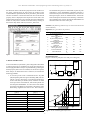
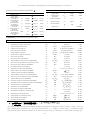
JOURNAL OF
Journal of Engineering Science and Technology Review 3 (1) (2010) 7-13
Engineering Science and
Technology Review
Research Article
www.jestr.org
Analysis of air-conditioning and drying processes using spreadsheet add-in
for psychrometric data
C.O.C. Oko* and E.O. Diemuodeke
Department of Mechanical Engineering, University of Port Harcourt, P.M.B 5323 Port Harcourt, Nigeria.
Received 6 October 2009; Accepted 23 December 2009
Abstract
A spreadsheet add-in for the psychrometric data at any barometric pressure and in the air-conditioning and drying temperature ranges was developed using appropriate correlations. It was then used to simulate and analyse air-conditioning and drying processes in the Microsoft Excel environment by exploiting its spreadsheet and graphic potentials. The package allows
one to determine the properties of humid air at any desired state, and to simulate and analyse air-conditioning as well as
drying processes. This, as a teaching tool, evokes the intellectual curiosity of students and enhances their interest and ability
in the thermodynamics of humid-air processes.
Keywords: Psychrometry, air-conditioning, drying, spreadsheet add-in, Microsoft Excel.
1. Introduction
Therefore, it is possible to develop computer procedures
in Visual Basic for Applications (VBA) for generating the psychrometric data as spreadsheet add-ins. Such a procedure would
then be used in the MS Excel environment for the simulation and
analysis of air-conditioning and drying processes in an interactive fashion and in a manner that fully exploits the spreadsheet
and graphic potentials of MS Excel. Such tool would assist the
design engineer in his work, especially when incorporated into a
larger plant design software. It would also be tool an easily affordable tool for the effective teaching of air-conditioning and drying
engineering principles to students of mechanical and chemical
engineering. The use of the MS Excel environment for enhancing the learning process in engineering is not new [6, 7, 8, 9].
Our experience has also shown that students exhibit greater interest, commitment and ability in using the spreadsheet for problem
solving, especially when graphical output is involved, than in the
traditional approach.
This paper, therefore, presents a spreadsheet add-in for the
psychrometric data for any barometric pressure and in the dry bulb
temperature range of 0 to 550 (0C), and uses it to illustrate the
interactive determination of the state properties of humid air, and
simulation and analysis of air-conditioning and drying processes.
The properties of humid air are very important in air-conditioning
and drying process analysis and system design. The property data
are usually provided as tables and charts of properties. But, reading
the psychrometric charts is strenuous, time consuming and always
prone to errors, and the use of property tables frequently requires
interpolation between the tabulated data, which is also manual and
time consuming activity. However, the proliferation of computer
technology in contemporary engineering practice ensures greater
speed and accuracy, and thus should limit or even eliminate the
use of property charts and tables in engineering analysis. The
present trend in engineering practice is, therefore, towards the development of computer packages that are capable of automatic
generation of the values of the desired thermodynamic properties,
and thus, facilitating their use in engineering analysis [1].
Many computer software packages are now available for engineering analysis, which have the facility for providing the thermodynamic properties of working fluids [1, 2]. But these packages
are not available in most computers; they must be bought and installed; they cannot be modified by their users, say, to account for
varying barometric pressure; special training is usually required
for their users; and internet connectivity may be necessary. But
these shortcomings can be overcome if computer packages that
are easy to develop, modify and exploit by users are available.
The Microsoft (MS) Excel offers a suitable environment for the
development of such packages [3, 4, 5].
2. Governing Equations
Following the works of [10, 11, 12], the basic psychrometric
properties are related as follows:
* E-mail address: [email protected].
ISSN: 1791-2377 © 2010 Kavala Institute of Technology. All rights reserved.
7
C.O.C. Oko and E.O. Diemuodeke / Journal of Engineering Science and Technology Review 3 (1) (2010) 7-13
Specific humidity (g):
The Carrier’s equation for the partial pressure of the water
vapour, Pwv, is given as
(1)
(7)
where Pb and Pwv are the barometric pressure and partial pressure
of the water vapour, respectively.
If the temperature of humid air (t) is higher than the temperature of saturation (ts) of water vapour (wv) at the dry air (da)
pressure (Pd.a), that is, t > ts , then Pwv = Pda and
where P(s)wb [kPa] is the saturation pressure at the wet bulb temperature.
Specific volume (v):
(1a)
(8)
where RH is the relative humidity of the air, given as
where T [K] is the absolute temperature of humid air, T = 273 + t
; t is temperature in degree celsius.
The humid air analysis is carried out using the following
algorithm:
(2)
where Ps is the saturation pressure of the water vapour.
start
input data:
Enthalpy of Moist Air (h):
(3)
where t, cpda , and cpwv are the dry bulb temperature, specific heat
capacity of the dry air, and specific heat capacity of the water vapour, respectively.
The average specific heat capacities are given, respectively
for air-conditioning and drying processes as cpda =1.005 (kJ/kgK)
and cpwv =1.88 (kJ/kgK), and cpda =1.01 (kJ/kgK) and cpwv =1.97
(kJ/kgK).
Wet Bulb Temperature (twb) and Thermodynamic Wet Bulb
Temperature (t* ):
i. obtain the prevailing barometric pressure;
ii.obtain the desired (unknown) property (specific enthalpy, dry bulb temperature, wet bulb temperature,
specific volume, specific humidity, relative humidity
or dew point temperature);
iii. obtain two known properties and their values;
compute (using the relevant relationships for the psychro-
metric properties) the specific humid volume, specific enthalpy, specific humidity, dry-bulb, wet-bulb or dew-point temperature;
output the desired data (property name and numerical value);
use the output for process simulation and analysis, if
desired;
plot psychrometric charts, if desired;
stop.
(4)
The software was developed in MS Excel Visual Basic for
Application Integrated Development Environment (Excel-VBA
IDE) as an Excel add-in, called Psychrometric_data, using all the
relevant correlations for the thermodynamic analysis of humid air,
given in the governing equations, and following the computational algorithm. Some of the procedures are iterative with an error
bound of 0.01%. The interface retrieves and supplies information
on any of the humid air properties. A command button control on
the Excel form is used to run the macro that implements a particular function.
After a successful installation of the Excel add-in, the Psychrometric_data menu is seen on the standard menu bar. By clicking on the Start button of the Psychrometric_data menu, the window shown in Figure 1 appears. Select the process type (Drying or
Air Conditioning) by clicking on the relevant OptionButton. If the
barometric pressure is different from the standard, Pb= 101.325
[kPa], check the No box, and enter the prevailing barometric pressure in the TextBox provided. Select the unknown property from
the ComboBox captioned Unknown Property. In the ComboBox
captioned Function, (…,…), select the known properties. Key in
and
t* = t −
h*fg
cp
(g* − g)
(5)
where
(6)
Le = 0.945 is the Lewis number for humid air, in which case
twb ≈ t* ; αα [W/m2K], kM [kgw.v / m2s], and cp [kJ/kgd.aK] are the
heat transfer coefficient of the air film around the wetted surface,
the mass transfer coefficient based on the specific humidity (g) and
the humid specific heat, respectively; h(fg)wb and gwv are the specific
latent enthalpy and specific humidity at the wet bulb temperature,
respectively; and Rda= 0.2873 [kJ/kgK] is the dry air gas constant;
the superscript “*” denotes adiabatic saturation properties and the
indices “fg” and “wb” denote latent conditions and wet bulb temperature, respectively.
8
C.O.C. Oko and E.O. Diemuodeke / Journal of Engineering Science and Technology Review 3 (1) (2010) 7-13
the numerical values of the known properties into the TextBoxes in
the Frame captioned Input the known data. By clicking on the
CommandButton captioned Read, the Psychrometric_data uses the
relevant correlations to obtain the numerical value of the desired
property, which is displayed in the Output Data Frame and is also
automatically transferred to a pre-selected cell in the worksheet for
further use. The process continues for another state by clicking on
the Continue drop menu of the Psychrometric_data menu.
ble and latent heat gains are 6 and 0.8 kW, respectively. The
performance of the dehumidifier (adsorbent material) is
characterized by the inlet and exit humidity ratios of the air
flowing through it, which are tabulated below. Assume the
heat of adsorption of moisture to be 390 kJ/kgw.v Determine
the volume flow rate of the air through the dehumidifier and
the heat transfer rate in the cooler [10].
Solution: (The following solution steps are carried out on the MS
Excel worksheet)
Input data: (the given data in the problem)
S/No
7
8
room latent heat
1
2
3
4
5
6
Figure 1. The add-in (Psychrometric_data) window.
Quantity
dry bulb temperature of
room
relative humidity of
room
dry bulb temperature of
outside air
wet bulb temperature of
outside air
volume flow rate of
outside air
dry bulb temp. of air
leaving the cooler
room sensible heat
Symbol
tdbi
Value
C
20
o
%
25
tdbo
o
C
40
twbo
o
C
25
m3/s
0.2
C
14
QRS
kW
6.0
QRL
kW
0.8
RHi
Vo
tdbs
o
Sketches/Diagrams:
(Figure 2 shows the plant flow sheet and process diagram).
3. Results and Discussion
As an Excel add-in, Psychrometric_data is designed to aid students
as well as practicing air conditioning or drying plant engineers in
their design/performance analysis by automatically providing the
desired property data in the environment, for the relevant spreadsheet analysis. To illustrate how this is achieved, we consider the
following problems:
1.A room for process work is maintained at 20oC dry bulb
(db) temperature and 25% relative humidity (RH). The outside air is at 40oC db and 25oC wet buld (wb) temperature.
Twelve cubic metre per minute (cmm) of fresh air is mixed
with a part of the recirculated air, and another passed over
the adsorption dehumidifier. It is then mixed with another
part of the recirculated air, and sensibly cooled in the cooler
before being supplied to the room at 14oC. The room sensiinlet humidity ratio, g1x103
[g/kgd.a]
2.86
4.29
5.70
7.15
8.57
10.00
11.43
12.86
14.29
Units
exit humidity ratio, g2x103
[g/kgd.a]
0.43
0.57
1.00
1.57
2.15
2.86
3.57
4.57
5.23
Figure 2. The air-conditioning plant and processes.
9
C.O.C. Oko and E.O. Diemuodeke / Journal of Engineering Science and Technology Review 3 (1) (2010) 7-13
(psychrometric data obtained using the add-in,
cp
kJ/kg
1.024
2
hfgref
kJ/kg
2500
75.760
3
reference temperature
tref
(tdbi,RHi)
29.010
4
Reference density
kgw.n/kgd.a
(tdbo,twbo)
0.014
5
gi
kgw.n/kgd.a
(tdbi,RHi)
0.003
6
vo
m /kgd.a
(tdbo,twbo)
0.907
RHo
%
(tdbo,twbo)
29.570
vi
m3/kgd.a
(tdbi,RHi)
0.835
Quantity
Symbol
1
wet bulb temperature of room
specific enthalpy
of outside air
specific enthalpy
of room air
specific humidity
of outside air
specific humidity
of room air
specific volume of
outside air
relative humidity
of outside air
specific volume of
room air
twbi
3
4
5
6
7
8
Data read from literature:
isobaric specific heat
capacity of air
Specific heat of
vaporization
S/No
2
(…,…)
Units
Function
Value
1
C
(tdbi,RHi)
11.210
ho
kJ/kgd.a
(tdbo,twbo)
hi
kJ/kgd.a
go
o
3
C
25
ρref
kg/m3
1.2
heat of adsorption
Qa
kW
390
Iteration error
ε
-
o
0.000005
Computation: (provides answers the questions asked)
S/No
Quantity
Symbol
Units
Function
Value
mo
kg/s
mo=Vo/vo
0.221
C
∆ts=tdbi-tdbs
6.000
Ks=ρrefcp(273+tref)
Vs=QRS(tdbs+273)/(KS∆tdbs)
0.784
1
mass flow rate of fresh air
2
temperature rise of supply air in the room
3
sensible volumetric heat constant
KS
kJ/m
4
volume flow rate of supply air
Vs
m3/s
5
Latent volumetric heat constant
KL
kJ/m3
6
specific humidity of supply air
gs
kgw.v/kgd.a
7
heat taken by the supply air per unit mass
qs
kJ/kg
qs=cp∆tdbs
6.144
8
mass flow rate of fresh air
ms
kg/s
ms=QRS/qs
0.977
9
mass flow rate of the recirculated air
mi
kg/s
mi=ms-mo
0.756
10
specific humidity of air at the inlet of the dehumidifier
g1
kgw.v/kgd.a
g1= φ(g1,ε)*
0.010*
11
mass flow rate of recirculated air mixing before the cooler
mi2
kg/s
mi2=mi-mi1
0.614
12
mass flow rate of air entering the dehumidifier
md
kg/s
md=ms-mi2
0.363
13
recirculation/fresh air mass mixing ratio
γi1,o
-
γi1,o=mi1/mo
0.644
14
temperature of air entering the dehumidifier
tdb1
C
tdb1=(tdbo+ζi1,otdbi)/(1+ζi1,o)
32.165
15
specific volume of air entering the dehumidifier
v1
m3/kgd.a
16
volume flow rate of air through the dehumidifier
17
specific humidity of air at the exit of the dehumidifier
18
mass flow rate of recirculated air before the dehumidifier
19
specific humidity drop in the dehumidifier
20
21
22
total heat transfer rate in the dehumidifier
23
temperature rise in the dehumidifier
24
∆tdbs
o
3
o
KL=ρrefhfgref(273+tref)
gs=gi-QRL(tdbs+273)/(KLVs)
(tdb1,g1)
366
894000
0.003
0.878
Vd
3
m /s
Vd=mdv1
0.318
g2
kgw.v/kgd.a
g2= -0.1273g1+0.00382
0.003*
mi1
kg/s
mi1=mo(g1-go)/(gi-g1)
0.142
∆gd
kgw.v/kgd.a
∆gd=g2-g1
-0.007
heat transfer rate due to condensation in dehumidifier
Qcond
kW
Qcond=2500mdI∆gdI
6.345
heat transfer rate due to adsorption of moisture in the dehumidifier
Qads
kW
Qads=QamdI∆gdI
0.990
Qd
kW
Qd=Qcond+Qads
7.335
C
∆tdbd=Qd/(mdcp)
19.756
C
tdb2=tdb1+∆tdbd
51.920
-
γi2,2=mi2/md
1.693
C
tdb3=(tdb2+γi2,2tdbi)/(1+γi2,2)
31.851
∆tdbd
o
temperature of air exiting the dehumidifier
tdb2
o
25
dehumidifier/recirculation air mass mixing ratio
γi2,2
26
temperature of air entering the cooler
tdb3
27
specific enthalpy of air entering the cooler
h3
kJ/kgd.a
28
specific enthalpy of the supply air
hs
kJ/kgd.a
29
heat transfer rate in the cooler
Qc
kW
o
(tdb3,gs)
(tdbs,gs)
Qc=msIhs-h3I
41.260
22.120
18.691
*
By curve fitting the experimental data for the dehumidifier performance using MS Excel curve fitting tool, we obtain g2 = 20.928 g21 + 0.08g1 - 7 x 10-5 = φ(g1),
Figure 3. Equating the last two equations, f(g1) = φ(g1), we get the iteration scheme, g1,j+1 = -100.989 g21,j + 0.01877. Setting g1,0 = 0.00286 and iterating in
Excel environment, within an absolute error bound of 10-5, we obtain the values of g1 and g2 as g1=0.0097 and g2= -0.1273g1+0.00382 =0.0027 (kgwv/kgda).
10
C.O.C. Oko and E.O. Diemuodeke / Journal of Engineering Science and Technology Review 3 (1) (2010) 7-13
Sketches/Diagrams:
(Figure 3 shows the plant flow sheet and process diagram).
Figure 3. Curve fitting of the dehumidifier data and solution of the equation f(g1)= φ(g1).
2.One tonne of some moist material is to be dried per hour from
an initial moisture content of uin = 50 [%] to a final moisture content of ufin = 6 [%] (wet basis). The temperature and
humidity of the outdoor air are to = 25 [%] and go = 0.0095
[kgw.v/kgd.a], respectively, and those of the air leaving the dryer
(spent air) are ts= 60 [oC] and gs = 0.041 [kgw.v/kgd.a]; where
the subscripts “wv” and “da” denote “water vapour” and “dry
air”, respectively. The drying of the moist material can be accomplished by any of the following three arrangements:
(a)The temperature of the outdoor air is raised in the heater before it enters the dryer; the humid air leaving the dryer (spent
air) is exhausted into the atmosphere.
(b) The temperature of the outdoor air is raised to 100 [oC] in
the heater; it enters the dryer and partially dries the moist
material; it then enters the reheater, where its temperature
is again raised to 100 [oC] before it is reintroduced into the
dryer to complete the drying process; the spent air is then
exhausted into the atmosphere.
(c)The outdoor air is mixed with 80 [%] recirculated; it is then
heated in the heater and introduced into the dryer to process the
moist material; the spent air is exhausted into the atmosphere.
Figure 4. The convective drying plant and processes.
Data read: (psychrometric data obtained using the add-in)
Determine the outdoor air flow rate through the dryer, and
the power consumption (heat transfer rate) for each of the drying arrangements. Also compare the drying potentials of these
arrangements [12].
Symbol Units
kg/s
initial moisture content of material
uin
-
0.5
3
final moisture content of material
ufin
-
0.06
4
temperature of air in case (b) heater
tdbb
C
100
5
fraction of recirculated air
-
0.8
6
outside air dry bulb temperature
tdbo
C
25
7
outside air specific humidity
go
8
spent air dry bulb temperature
tdbs
9
spent air specific humidity
gs
initial mass of moist material
2
o
κ
o
C
Value
Value
1
ho
kJ/kgda
(tdbo,go)
46.25
hs
kJ/kgda
(tdbs,gs)
168.13
RHo
%
(tdbo,go)
43.33
RHo
%
(tdbs,gs)
31.09
C
(tdbs,gs)
39.8
C
(go,hs)
139.1
kgwv/kgda
(tdbs,hs)
0.02528
C
(tdbb,go)
34.68
5
0.278
6
7
8
kg/kgd.a 0.0095
o
Units
4
Value
mmm
1
Symbol
3
Input data: (the given data in the problem)
Quantity
Quantity
outside air specific
enthalpy
spent air specific
enthalpy
outside air relative
humidity
spent air relative
humidity
spent air wet bulb
temperature
case (a) heated air
dry bulb temperature
specific humidity of
air in the first process O-1b-2
case (b) heated air
wet bulb temperature
2
Solution: (The following solution steps are carried out on the MS
Excel worksheet)
S/No
S/No
60
kg/kgd.a 0.041
11
twbs
o
tdba
o
g2
twbb
o
C.O.C. Oko and E.O. Diemuodeke / Journal of Engineering Science and Technology Review 3 (1) (2010) 7-13
Computation: (Answers the question asked)
S/No
(a)
1
Quantity
Symbol
Units
Formula
Value
rate of moisture removal in the dryer
mwv
kg/s
mwv=mmm(uin-ufin)/(1-ufin)
2
rise in the specific humidity of the working fluid (air) in the dryer
∆g(a)
kgwv/kgda
∆g(a)=gs-go
0.0315
3
mass of dry air per kilogram of moisture evaporated
x(a)
kgda/kgwv
x(a)=1/∆g(a)
31.74603
4
mass flow rate of dry outdoor air through the dryer
mo(a)
kgda/s
mo(a)=mwv*x(a)
4.131037
5
change in the specific enthalpy of air
∆h(a)
kJ/kgda
∆h(a)=hs-ho
6
heat consumption per kilogram moisture evaporated
q(a)
kJ/kgwv
q(a)=x(a)*∆h(a)
3869.206
power consumption
Q(a)
kW
Q(a)=mwv*q(a)
503.4908
∆gib2
kgwv/kgda
∆gib2=g2-go
0.01578
9
rise in the specific humidity of the air during the first pass through the
dryer, process O-1b-2
mass of dry air per kilogram of moisture evaporated in the first process
x(b)
kgda/kgwv
x(b)=1/∆g(b)
63.37136
10
mass flow rate of dry outdoor air through the dryer
mo(b)
kgda/s
mo(b)=0.5*mwv*x(b)
4.123183
11
change in the specific enthalpy of air
∆h(b)
kJ/kgda
∆h(b)=hs-ho
12
heat consumption per kilogram moisture evaporated
q(a)
kJ/kgwv
q(b)=x(b)*∆h(b)
7723.701
Q(b)
kW
Q(b)=0.5*mwv*q(b)
502.5336
g4
kgwv/kgda
g4=(1-κ)go+κ*gs
0.0347
∆g(c)
kgwv/kgda
∆g(c)=gs-g4
0.0063
7
(b)
8
0.130128
121.88
121.88
13
power consumption
(c)
14
specific humidity of air after mixing of the outdoor and recirculated air
15
rise in the specific humidity of air in the dryer
16
mass of dry air per kilogram of moisture evaporated
x(c)
kgda/kgwv
x(c)=1/∆g(c)
158.7302
17
mass flow rate of dry air through the dryer
m4
kgda/s
m4=mwv*x(c)
20.65518
18
mass flow rate of dry outdoor air through the dryer
mo(c)
kgda/s
mo(c)=(1-κ)*m4
4.131037
19
specific enthalpy of air after mixing
h4
kJ/kgd.a
h4=(1-κ)ho+κ*hs
143.754
20
change in the specific enthalpy of air
∆h(c)
kJ/kgda
∆h(c)=hs-h4
24.376
21
heat consumption per kilogram moisture evaporated
q(c)
kJ/kgwv
q(c)=x(c)*∆h(c)
3869.206
22
power consumption
Q(c)
kW
Q(c)=mwv*q(c)
503.4908
23
"big" wet bulb depression for (a)
∆tB(a)
K
∆tB(a)=tdba-twbs
99.3
24
"small" wet bulb depression for (a)
∆tS(a)
K
20.2
25
drying potential (logarithmic mean temperature difference (LMTD)) for (a)
∆tp(a)
K
26
drying potential relative to that of (a)
εa(a)
%
∆tS(a)=tdbs-twbs
∆tp(a)=(∆tB(a)-∆tS(a))/
(ln(∆tB(a)/∆tS(a)))
εa(a)=(∆tp(a)/∆tp(a))*100
27
"big" wet bulb depression for (b), first pass through the dryer
∆tB(b),1
K
∆tB(a),1=tdbb-twbb
65.3
28
"small" wet bulb depression for (b), first pass through the dryer
∆tS(b),1
K
25.3
29
drying potential (LMTD) for (b), first pass
∆tp(b),1
K
30
"big" wet bulb depression for (b), second pass through the dryer
∆tB(b),2
K
∆tS(a),1=tdbs-twbb
∆tp(b),1=(∆tB(b),1-∆tS(b),1)/
(ln(∆tB(b),1/∆tS(b),1))
∆tB(a),2=tdbb-twbs
31
"small" wet bulb depression for (b), second pass through the dryer
∆tS(b),2
K
20.2
32
drying potential (LMTD) for (b), first pass
∆tp(b),2
K
36.7
33
drying potential for (b)
∆tp(b)
K
∆tS(a),2=tdbs-twbs
∆tp(b),2=(∆tB(b),2-∆tS(b),2)/
(ln(∆tB(b),2/∆tS(b),2))
∆tp(b)=0,5 *(∆tp(b),1+∆tp(b),2)
34
drying potential relative to that of (a)
εa(b)
%
εa(b)=(∆tp(b)/∆tp(a))*100
79.5
35
dry bulb temperature of air after the heater for (c)
tdbc
o
36
"big" wet bulb depression for (b), first pass through the dryer
∆tB(c)
K
∆tB(c)=tdbc-twbs
33.5
37
"small" wet bulb depression for (b), first pass through the dryer
∆tS(c)
K
20.2
38
drying potential (LMTD) for (c)
∆tp(c)
K
39
drying potential relative to that of (c)
εa(c)
%
∆tS(c)=tdbs-twbs
∆tp(c)=(∆tB(c)-∆tS(c))/
(ln(∆tB(c)/∆tS(c)))
εa(c)=(∆tp(c)/∆tp(a))*100
12
C
(g4,hs)
49.7
100
42.2
60.2
39.5
73.25
26.3
52.92
C.O.C. Oko and E.O. Diemuodeke / Journal of Engineering Science and Technology Review 3 (1) (2010) 7-13
and participation in students, and its graphic, equation-solving and
curve-fitting capabilities permit the student to visualise the humid
air processes and appreciate the scope and applications of thermodynamics of humid air. Comparism of process characteristics is
relatively simple, and process simulation under a range of varying
input parameters is always possible as in Figure 5, which shows
The results of the solutions of the illustrative problems 1 and
2 using the add-in are in good agreement with those obtained by
[10] and [12], respectively. The psychrometric data provided by the
add-in are in agreement with those from the psychrometric charts
for air-conditioning processes and drying processes [12] and [13],
respectively. It was, however, observed that the maximum relative
deviation of 4.5% occurs in the values of the specific enthalpy;
but this is within an acceptable limit for most applications. The
interactive nature of the MS Excel environment evokes curiosity
the dependence of the outdoor dry air mass flow rate (m o ( c ) ) , mass
flow rate of air through the dryer ( m 4 ) and drying potential (∆t p ( c ) )
on the fraction of dryer spent air recirculated (κ).
4. Conclusion
The spreadsheet add-in is provided in an easily accessible MS Excel environment to facilitate process analysis and simulation efforts of students as well as practising air-conditioning and drying
engineers. Our experience has shown that students exhibit greater
interest, commitment and ability in using the spreadsheet for problem solving, especially when graphical output is involved, than in
the traditional approach. The tool proposed in this paper is easy to
install, use and modify by engineering students in any computer
driven by the MS Office. It is, therefore, strongly recommended
as a teaching tool for engineering students, especially in localities
with limited access to internet facilities, which may offer alternative tools online.
Figure 5. Variation of outdoor air flow rate (mo(c)), mass flow rate of air
through the dryer (m4) and drying potential (∆tp(c)) as function of
fraction of dryer spent air recirculated (κ), Problem 2(c).
References
1. Beckmanand W. and Klein S. (1996), Engineering Equation Solver (EES)
User manual, McGraw Hill, N Y.
2. Lemmon E. W., Huber M. L. and McLinden M. O. (2002), Refprop Version 7.0 User Guide, U.S NIST Department of Commerce.
3. Deane A. (2005), Developing Mathematics Creativity with Spreadsheets,
J. of Korea Society of Math. Educ., Series D: R. in Math. Educ. 9 /3 187201.
4. Deane A., Erich N. and Robert S. S. (2005), Mathematical Modelling and
Visualization with Microsoft Excel, KAIST, Retrieved April 26th, 2006
http://www.mathnet.or.kr/kaist2005/article/arganbright.pdf.
5. Liengme V. B. (2000), A Guide to Microsoft Excel For Scientist and Engineers. Woburn, Butterworth Heinemann.
6. Schumack M. R. (1997), Teaching heat transfer using automation-related
case studies with a spreadsheet analysis package, Int. J. Engineering Education, 25 177-196.
7. Lira C. T. (2000), Advanced Spreadsheet Features for Chemical Engineering Calculations, Submitted to Chem. Eng. Educ., Retrieved March 22nd,
2009 http://www.egr.edu/~lira/spreadsheats.pdf
8. Viali L. (2005), Using spreadsheets and Simulation to Enhance the Teaching of Probability and Statistics to Engineering Students, Int. Conf. on
Eng. Educ., Poland, July 25-29th, (Silesian University of Technology,
Gliwice).
9. Whiteman W. and Nygren K. P. (2000), Achieving the Right Balance: Properly Integrated Mathematical Software Packages into Engineering Education, J. of Enging Educ., 89/ 3 pp. 331-336.
10. Arora, C. P. (2000), Refrigeration and Air Conditioning. Tata McGrawHill, New Delhi.
11. Akpan, I. E. (2000), Analysis of Psychrometric Data for the Niger-Delta
Region of Nigeria. A thesis in Mechanical Engineering for the award of
M. Eng. University of Port Harcourt, Port Harcourt.
12. Pavlov, K. F et al. (1979), Examples and problems to the course of unit
operations of Chemical Engineering. Mir, Moscow.
13. Eastop, T. D and McConkey, A. (1993), Applied Thermodynamics: For
Engineering Technology. Fifth edition, Pearson Education, New Delhi.
13