Download Signal Processing and Control

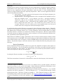
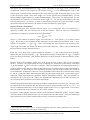
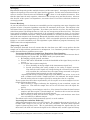
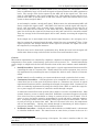
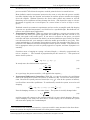
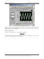
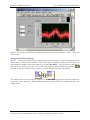
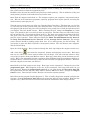
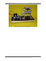
University of California at Berkeley
Physics 111 Laboratory
Basic Semiconductor Circuits (BSC)
Lab 11
Signal Processing and Control
©2007 by the Regents of the University of California. All rights reserved.
Reading:
Wells & Wells
Entire Book on LabView.
Horowitz & Hill
Chapter 15
Press, Teukolsky, Vetterling and Flannery
Chapters 12, 13 and 15.5
Numerical Recipes 1
LabVIEW Analysis Concepts Manual Chapters 3 and 4. ( Located in the BSC Share)
LabVIEW PID Control Toolset User Manual Chapters 1-4. ( Located in the BSC Share)
In this lab you will learn how to extract signals from noise, and how to use a PID controller.
Several LabVIEW programs are mentioned in this lab writeup. Many of these programs can be
downloaded from http://socrates.berkeley.edu/~phylabs/bsc/LV_Programs/ and can also be found on
your lab computers in \\Atlas2\D$\111 Lab\BSC Share\ Two versions of the programs are
typically available for download: an executable version that should run without LabVIEW (but requires a large download from National Instruments, which should occur automatically, and only
needs to be done once) and should run on PC’s, Mac’s and Linux boxes; and the original LabVIEW
source code which requires LabVIEW. The LabVIEW Analysis Concepts Manual can be downloaded
from \\Atlas2\D$\111 Lab\BSC Share\LAB_11
Pre-lab questions:
1. You seek to detect a signal of intrinsic frequency spread Δf = 10 Hz with a room temperature detector that has an impedance of 1000ohms. You sample for 10mS. What is the smallest signal
that you can detect?
Background
Signal Processing Overview
Most real world signals are contaminated by noise. A frequently used figure-of-merit is the signalVSignal
. The S n for clean signals is much larger than one; as S n approaches one the
to-noise ratio, S n =
VNoise
signal fades into the noise, as shown in the figure below:
1
This book (available in several versions for different computer languages), is the standard references on numerical algorithms. Like Horowitz & Hill, it is informative, chatty, opinionated and
funny. Almost all physicists own a copy. Chapters of the book can be downloaded free from
http://library.lanl.gov/numerical/index.html This book is listed as a supplement; read it if you want
to learn more about the numerical techniques.
Last Revision: August 2007
©2007 Copyrighted by the Regents of the University of California. All rights reserved.
Page 1 of 22
Physics 111 BSC Laboratory
Lab 11 Signal Processing and Control
Fortunately, we can often extract the signal from the noise. There are three primary techniques for
recovering the signal:
1. Bandwidth narrowing.
2. Averaging.
3. Pattern matching.
There are many ways to implement each of these techniques; we will explore the most important.
Bandwidth Narrowing
Generally, signals are narrow band, while noise is either wide band (like Johnson noise) or narrow
band (like 60Hz hum), but of a different frequency than the signal frequency. By narrowing the
bandwidth of the signal we can diminish the noise, thereby improving the signal-to-noise ratio. For
example, it is not uncommon to detect a sine wave of frequency f and amplitude A that has been contaminated by Johnson noise. The signal-to-noise ratio will be
Sn =
A
4k B RTB
,
where B is the bandwidth that we accept. Making B small will increase the signal-to-noise ratio; if
we could make B arbitrarily small, we could recover any size signal. Unfortunately, we cannot make
B arbitrarily small as there are at least two limits on the size of B :
1. All signals have some intrinsic frequency spread, Δf , and the bandwidth cannot be made
smaller than this spread.
2. The accuracy to which a signal frequency can be determined is inversely proportional to the
length of time that you measure the signal, or, alternately, to the number of waveform cycles
N that are contained in your sample. For example, assume you anticipate measuring a signal near 1kHz, and you sample the signal for 100mS. You would collect approximately 100
cycles in this time. Thus, you cannot determine the frequency of what you measure to better
than about 1 N = 1% of 1kHz, or 10Hz, nor can you make the bandwidth any smaller. (The
derivation of this uncertainty relation is given below.)
The two most important Bandwidth narrowing techniques are filtering and Fourier Transforming.
Filtering narrows the bandwidth directly, attenuating the out-of-band noise. Fourier Transforming
also narrows the bandwidth, but by a more subtle method. While it does not attenuate the noise, it
allows you to concentrate on the narrow portion of the spectrum that contains your signal, thereby
ignoring the majority of the noise which is spread through the entire spectrum.
Last Revision: August 2007
©2007 Copyrighted by the Regents of the University of California. All rights reserved.
Page 2 of 17
Physics 111 BSC Laboratory
Lab 11 Signal Processing and Control
Filtering
Filtering is best used for real-time signals 2 and can be implemented in analog or digital (software).
Analog filters can be quite simple, can work quite well, and are often sufficient. But sharp analog
filters are very complicated, and most analog filters cannot be tuned; i.e. their rolloff frequencies
cannot be changed without physically replacing components. 3 There are some applications that demand analog filters, for instance:
• Anti-aliasing. You must attenuate the frequencies above the Nyquist frequency before the signal has been digitized.
• Amplifier chains. It is not uncommon for noise to swamp the later amplifiers in the a
high gain amplifier chain. 4 If, for instance, you have a 1μ V signal masked by
100μ V noise, and you use an amplifier chain with a gain of one million, the noise
would be amplified to 100V , saturating the final amplifier which is unlikely to be
able to output much more than ±10V . You would not be able to detect your now
1V signal. However, if you use a filter early in your amplifier chain, you can get rid
of most of the noise, and prevent it from saturating the chain.
In applications where analog filtering is not required, digital filtering is often superior. Digital filters are far more flexible, can be made arbitrarily sharp, are trivially tunable, and their topology
(RC, Butterworth, Chebyshev, Bessel, etc.) is easily changeable. However digital filters are computationally intensive, and their use is limited to relatively low frequencies. Moreover, digital filters
necessarily operate on digitized waveforms, and are subject to all of the limitations (Nyquist theorem, quantization) of the digitization process.
Digital filters are difficult to design. Fortunately, there are many canned routines available, including an extensive suite in LabVIEW. We need not worry too much about the differences between the
types of digital filters; refer to Chapter 3 of the LabVIEW Analysis Concepts manual for more information. In particular, Figure 3.25 of this reference shows a handy flowchart for picking the correct
filter type.
Fourier Transforms
Fourier transforms find the spectral content of a signal: the amplitude and phase of the signal as a
function of frequency. You are all familiar with Fourier series from your math and physics classes;
Fourier transforms are quite similar. In a Fourier series, you consider only the harmonics of the periodic wave of period T that you are analyzing:
T
⎛ 2π n ⎞
An = ∫ f (t ) sin ⎜
t ⎟ dt
⎝ T ⎠
0
In taking the Fourier transform, you analyze all times and all frequencies:
F (ω ) =
∞
∫
f (t )e − jω t dt
−∞
The Fourier transform of a sinusoid is a delta function centered at the frequency of the sinusoid.
2
Real-time signals are those which you receive as in infinite train of periodic samples, and which
you wish to analyze as your receive each sample. Other techniques, like Fourier Transforms, can be
better when you receive your entire sample before you begin processing.
3 Tunable filtering can be achieved by multiplying an incoming signal, at frequency f , by a variable
frequency sine wave at frequency f 0 . The beat frequency at f − f 0 is then passed through a sharp,
fixed frequency filter. The filter is tuned by changing f 0 . This common technique is called superheterodyning, and is used in most radios and TVs. See http://en.wikipedia.org/wiki/Superhet
4 A series of amplifiers in which each amplifier is fed by the output by the previous amplifier in the
chain.
Last Revision: August 2007
Page 3 of 17
©2007 Copyrighted by the Regents of the University of California. All rights reserved.
Physics 111 BSC Laboratory
Lab 11 Signal Processing and Control
In the real world, any sample has a finite length; consequently, the Fourier transform becomes
T
1
F (ω ) = ∫ f (t )e − jω t dt
T 0
Here T is the length of the sample, not the period of the wave as it was for a Fourier series. The
sample may include many wave periods. The transform of a sinusoid with frequency ω0 is
F (ω ) =
=
T
1 jω0t − jω t
e e
dt
T ∫0
(
)
1
j ω −ω T
e ( 0 ) −1
j (ω 0 − ω ) T
The magnitude of this transform for a wave with frequency ω 0 = 2 and T = 8 is:
Instead of the delta function at ω 0 = 2 that we would get from an infinitely long sample, the transform is a finite-width pulse centered at ω 0 = 2 . The width of the pulse (to the first zeroes) is easy to
find if we assume that ω = ω 0 + Δω . Then
F (ω ) =
−1
( e− jΔωT − 1) .
j ΔωT
The first zeroes of this function occur at ΔωT = 2π , or Δω ω 0 = 1 f 0T = 1 Ν , where ω 0 = 2π f 0 and Ν is
the number of cycles of the wave in one sample. Because the pulse width is finite, we cannot readily
determine the precise frequency of the original signal. Consider a signal that is actually the sum of
two equal amplitude sine waves of frequency ω0 − Δω and ω0 + Δω . The plots below show this signal, in green, compared to a pure signal of frequency ω0 , in red, for various values of Δω .
Last Revision: August 2007
©2007 Copyrighted by the Regents of the University of California. All rights reserved.
Page 4 of 17
Physics 111 BSC Laboratory
Lab 11 Signal Processing and Control
The spectra are indistinguishable for Δω ω 0 = 0.025 , and nearly so for Δω ω 0 = 0.05 . Aside from an
unimportant change in the amplitude, the spectra for Δω ω 0 = 0.1 are distinguishable only by the
details of the secondary peaks surrounding the main peak; the width of the main peak is very close
to that of the pure signal. Only when Δω ω0 = 0.2 are the spectra easily distinguishable. Yet the
untransformed original signals are readily distinguishable. Thus, given only the spectrum, we cannot determine the frequency to better than about Δω ω 0 = 0.1 : one quarter of the width to the first
zero calculated above. In essence, we have an uncertainty principle: the longer we sample a signal
(the greater the time uncertainty), the better we know the frequency of the signal.
Discrete Fourier Transforms
The expression given above assumes that the signal, f (t ), is continuous. Since our signals are acquired by an ADC, they are actually sets of discrete samples. Thus, we must use a summation
rather than an integral to calculate the Fourier Transform: 5
N −1
F (k ) = ∑ f (n)e−2π jnk N ,
n=0
where N is the number of samples, taken over some time T ; each sample f (n) is taken at time
nT N . By analogy to the argument of the exponential in the continuous transforms, each k corresponds to a frequency f = ω 2π = k T . Thus, discretizing the time discretizes the frequency into
steps of 1 T ; the longer the sample, the better resolved the frequency. (This is just a restatement of
the uncertainty principle discussed above.)
From Lab 11, we know that a signal sampled at frequency f s = N T cannot represent a frequency
higher than the Nyquist frequency, f s 2 . The Nyquist frequency corresponds to k = N 2 . No higher
k has any physical meaning. (The Nyquist Theorem is actually derived via Discrete Fourier Transforms.)
Discrete Fourier Transformers would have little practical value if they could not be evaluated
quickly. Casually, one might think that the evaluating the transform would require evaluating
N 2 2 exponentials: N 2 for each of the N samples. Thus, the transform of a signal represented by a
100,000 samples would appear to take 10,000 times longer to evaluate than a signal represented by
1000 samples. As the accuracy of the transform increases with the sample length, this would be
very unfortunate. Fortunately, there are clever algorithms which reduce the evaluation time scaling
to N ln 2 N : a 100,000 sample representation takes only 665 times longer than a 1000 sample representation. These algorithms are called Fast Fourier Transforms, or FFTs. They are generally attributed to J. W. Cooley and J. W. Tukey, who published an implementation in 1965, but many others, including Gauss, had discovered similar algorithms.
The FFT algorithm works most naturally on samples lengths which are powers of 2. However sample lengths which are factorable into the products of powers of small primes, such as N = 2m 3k 5 j , can
also be transformed efficiently; stick to sample lengths which can be so represented. If necessary,
pad your sample with zeros to extend it to one of these lengths.
In practice, sample lengths below one million can be converted remarkably quickly. Longer sample
are slower than would be predicted by N ln 2 N scaling because of cache misses. Once the sample gets
large enough to require virtual memory disk accesses, conversion is painfully slow.
5
The convention used here has no overall multiplying constant; other conventions are used that
multiply this expression by some factor related to pi.
Last Revision: August 2007
Page 5 of 17
©2007 Copyrighted by the Regents of the University of California. All rights reserved.
Physics 111 BSC Laboratory
Lab 11 Signal Processing and Control
Averaging
Experiments frequently produce multiple instances of the same signal. Averaging the instances can
improve the signal-to-noise ratio if the signal itself is repetitive, and the noise uncorrelated from instance to instance. Then the noise will diminish as 1 N , where N is the number of instances. Note
that the signal must be truly repetitive, otherwise it will average away just like the noise. Also note
that because of the square root dependence, successive factor of two noise reductions becomes increasingly painful.
Pattern Matching
As you saw in Exercise 10.2, humans are remarkably good at recognizing some sorts of signals in the
presence of noise. Computer algorithms exist that can sometimes do the same. The simplest is the
well-known linear least squares algorithm. If you know your data lies on a line, why retain the individual data points? By fitting the data to a line you can average most of the noise away. The linear
least squares algorithm is easily generalized to fit polynomial coefficients to data, or even linear
combinations of nonlinear functions. More powerful methods are needed to fit nonlinear equations.
One of the most common is the Levenberg-Marquardt algorithm, which will fit one or more unknown
coefficients in a nonlinear expression to a data set. Given a reasonable guess for the unknown coefficients, it can work remarkably well. The algorithm is quite difficult to program; fortunately, LabVIEW comes with an implementation.
“Improving” your ADC
The techniques discussed above all assume that the data from your ADC is near perfect: that the
sample rate is high and that quantization is unimportant. It is sometimes possible to improve your
sample data when these conditions are not met.
Increasing the Effective Sample Rate: Equivalent Time Sampling
A technique called equivalent time sampling (ETS) can sometimes be used to increase the effective sampling rate of your ADC. For ETS to work, your system must:
1. Be sampling a rigidly periodic waveform.
2. Use an ADC whose bandwidth exceeds the bandwidth of the signal that you wish to
recover.
3. Use an ADC that acquires samples by:
a. First, obtaining an analog sample of the instantaneous signal level.
b. Second, presenting this analog sample to the analog to digital converter.
Note that the actual signal may change during the conversion time, but this
will not affect the conversion since the signal being converted is the previously obtained analog sample, not the current signal.
Acquiring and storing an analog sample may seem difficult, but, in fact, is easy to do
with a common circuit called a sample and hold. On command, the sample remembers the analog value at its input, typically by storing the value in a capacitor.
If your system does meet these requirements, you can acquire an accurate sample of a waveform by following these steps.
1. After receiving a trigger indicating the beginning of your waveform, acquire one
sample set. Note that the sample rate can be well less than twice the signal frequency.
2. After receiving a second trigger, wait for a delay interval less than the time between
samples, and then acquire a second sample set. Interleave this second set with the
first set, offsetting each point by the initial interval.
3. After receiving a third and successive triggers, acquire and interleave more data
sets, each offset by a different amount.
The offsets can be evenly and incrementally spaced, or can be random.
Increasing the resolution: Dithering
ADCs add quantization noise to low level signals. For example, the near-zero levels of a 10
bit ADC, with a range of ±10V, are -59, -39, -20, 0, 20, and 59mV. The ADC cannot represent
signals in between these levels. This is particularly problematic for signals that are less
than 10mV; the ADC will convert the signal to the constant 0mV, and the signal will disapLast Revision: August 2007
©2007 Copyrighted by the Regents of the University of California. All rights reserved.
Page 6 of 17
Physics 111 BSC Laboratory
Lab 11 Signal Processing and Control
pear entirely. Paradoxically, adding random noise will improve the conversions. If the
noise is sufficiently large, it will cause the signal to fluctuate between the ADC quantization
levels. The average of the levels reported by the ADC will be the signal level. This technique is called dithering, and is quite commonly used. Noise adding circuitry may be incorporated in the ADC, or you may have to add noise yourself. Often, the natural noise in your
system is often enough to dither.
As and example, consider a steady 9mV signal. Without noise, the aforementioned ADC will
always convert this signal to 0mV. Add 10mV noise however, and the signal will range between -1mV and 19mV, with occasional larger excursions. Roughly eleven times out of
twenty, the signal will be between -1 and 10mV and will be converted to zero, while nine
times out of twenty the signal will be between 10 and 19mV and will be converted to 20mV
Thus, the average of the converted signals will be 9mV, thereby recovering the original signal level.
If the sample rate is much higher than the desired signal frequency, the averaging can be
done by passing the converted signal through a digital low pass or smoothing 6 filter. If the
signal is periodic, and multiple instances of the signal are available, the signal can be further improved by averaging the instances.
The ideal noise level is about half a quantization step. Below this noise level the signal will
not fluctuate between steps, and above this level the noise itself introduces error.
Control
Most modern experiments are controlled by computers: computers set magnetic field levels, regulate
temperatures, move probes, control timing, open valves, turn on sources, etc. Control functionality
can be simple or complicated; the list below describes some of the most common control methodologies:
• On/Off Controllers. Epitomized by a light switch, a typical experimental function would be
controlling the state of a vacuum valve. On/off controls are trivial to program; they are usually implemented by controlling the state of a digital bit, which in turn, controls an electronic
switch.
•
•
On/Off controls are all or nothing; you cannot use them to reach a particular level or state.
Continuous Controllers. A stovetop burner valve exemplifies of a continuous control; a
control that lets us set the state of the driven object to a continuous set of levels. A typical
experimental function would be controlling the strength of a magnetic field. Continuous controls are commonly implemented by using the voltage from a DAC to control the target device: a power supply, for instance to control the current through a magnet.
A continuous control allows some systems, like a magnet, to reach a well defined state. Most
systems, however, are not so strictly controlled. Sometimes a system will appear to be stably
set to some level, but a perturbation or change in system can run it out of control. For instance, a stove top burner cannot be programmed to reach and hold a particular temperature. Temporary control can be achieved by setting a pot of water on stove burner. The water and pot will get no hotter than 100C. But once the water boils away, the temperature
will rise uncontrollably. Having once melted through an aluminum pot, which requires a
temperature of 660C, I am all too familiar with this scenario.
Feedback Controllers. A feedback control adds feedback to a On/Off control; a thermostat
is a familiar feedback control. The control turns on some device (a heater in the case of a
6
A smoothing filter outputs a running average of its inputs. Its action is similar to that of a low
pass filter.
Last Revision: August 2007
Page 7 of 17
©2007 Copyrighted by the Regents of the University of California. All rights reserved.
Physics 111 BSC Laboratory
Lab 11 Signal Processing and Control
thermostat) until some setpoint 7 is reached. Then the control turns off the device until the
process variable7 falls below the setpoint, at which point the device is turned back on.
Most feedback controls incorporate hysteresis; they turn on only after the process variable
has fallen slightly below the setpoint, and remain on until the process variable rises slightly
above the setpoint. Without hysteresis, the device under control may stutter on and off.
Stuttering can be inefficient and may damage the device. (The hysteretic range on a house
thermostat is typically one or two degrees; on a water heater it can be as large as 15 degrees.)
•
Feedback controls are common in experiments and are used to accomplish tasks like keeping
a process at a specified temperature, or a fluid level at a specified height. But feedback controls are too crude for many applications.
Proportional Controllers. When you merge onto a highway, you gun your engine in the
acceleration lane until your speed approaches the traffic speed, and then ease off as you
match your speed to the traffic speed. If you were to accelerate at low power, you would
reach the end of the acceleration lane before you attained sufficient speed, and if you did not
ease off toward the end, your attempt to match the traffic speed would be very jerky. This
control methodology is an example of proportional control; the strength of the drive is proportional to the difference between the setpoint and the process variable. Proportional control is appropriate when you wish to quickly approach a setpoint, and then asymptote to it
smoothly.
Consider a mass m hanging on a spring k of natural length y0 , driven by a proportional control to a setpoint ys . The constant of proportionality for the control is C . The equation of
motion for the system is:
d2y
= −mg − k ( y − y0 ) − C ( y − ys )
(1.1)
dt 2
In steady state, the solution of this equation is
ky
mg
1+ 0 −
Cys cys
y = ys
(1.2)
k
1+
C
As C gets large, the process variable y will approach the setpoint ys .
Proportional-Differential Controllers. While Eq. 1.2 correctly predicts the equilibrium
state of the spring-mass system, the system, as modeled by Eq. 1.1, will never reach equilibrium. Because the system possesses inertia (the m d 2 y dt 2 term in the equation of motion),
it will oscillate around the equilibrium. To satisfactorily control the system, we need to add
damping:
d2y
d
m 2 = −mg − k ( y − y0 ) − C ( y − ys ) − 2CTd ( y − ys ) .
(1.3)
dt
dt
Note the damping constant, Td , has units of time. The system is critically damped when
m
•
k +C
,
(1.4)
C2
and the system will converge to the setpoint quickly if it is near critical damping. However,
critical damping is not always the best choice; if some ringing can be tolerated, the system
will react more quickly if it is underdamped:
Td = m
7
Two definitions will clarify this discussion: A process variable is some measured value that characterizes the system; the setpoint is the desired level of the process variable.
Last Revision: August 2007
Page 8 of 17
©2007 Copyrighted by the Regents of the University of California. All rights reserved.
Physics 111 BSC Laboratory
Lab 11 Signal Processing and Control
If the system has some initial momentum, critical damping can lead to overshooting. If overshooting cannot be tolerated, the system must be overdamped:
The inertia in mechanical systems is explicit, but even non-mechanical systems exhibit inertia-like phenomena. For instance, thermostatically controlled heating systems have a form of
inertia. Typically, the thermostat is not immediately adjacent to the heater. When the temperature at the thermostat exceeds the setpoint, the thermostat will turn the heater off, but
the area near the heater will be warmer than the area near the thermostat. Heat will
spread away from the heater, and the temperature at the thermostat will continue to rise,
until the temperature equalizes everywhere. Thus, the system has inertia just like the
spring-mass system.
In general, any system with time delays will have inertia-like properties. Adding damping
through a differential term is frequently beneficial.
•
Proportional-Integral-Differential Controllers. From Eq. 1.2, we see that for any finite
C , the equilibrium is shifted away from the setpoint. If we need to hit the setpoint precisely,
we can add an integral term:
t
d2y
d
C
(1.5)
m 2 = − mg − k ( y − y0 ) − C ( y − ys ) − 2CTd ( y − ys ) − ∫ ( y − ys )dt.
dt
Ti 0
dt
The integral term integrates the difference between the process variable and the set point,
and drives this error to zero. Like Td , the integral constant Ti has units of time.
The proportional-integral-differential controller, or PID controller, generally works very
well, and is used in many systems. It is not limited to systems modeled by linear second or-
Last Revision: August 2007
©2007 Copyrighted by the Regents of the University of California. All rights reserved.
Page 9 of 17
Physics 111 BSC Laboratory
Lab 11 Signal Processing and Control
der differential equations like Eq. 1.5. For instance, the linear error, e = y − ys used in Eq. 1.5
can be replaced by any odd function of e.
The most difficult step in deploying a PID controller is determining the constants C , Td , and
Ti . There is no foolproof method that always gives the best values. For that matter, there is
no single set of “best values;” the best values depend on the desired response time, and your
ring and overshoot tolerances. If the system is very simple you may be able to calculate the
values, otherwise you will have to guess them or find them by trial and error. Once you get
values that keep the system stable, you may be able to use various algorithms 8 to optimize
them. Some of these optimization algorithms are available in LabVIEW. Finding the appropriate constants is called tuning the PID.
Practical PID controllers work by calculating the error, e = y − ys , between the process variable y and the setpoint, integrating and differentiating the error, scaling by the appropriate
constants, and summing to get a drive signal. PIDs can be implemented in analog or digital.
Analog PIDs output a continuous voltage. Digital PIDs operate in a loop: they measure the
process variable, compute the drive and output it with a DAC, and loop back to measuring
the process variable. Consequently, the drive from a digital PID is a series of steps.
Whether implemented in analog or digital, the system has a finite response time. If analog,
the response time is set by the bandwidth of the circuitry. If digital, the response time is set
by the speed of the ADC and DAC, the computation time of the calculation, and by any other
tasks that might be running on the processor that distract the processor’s attention. The
sum of all these times is called the service interval.
As a rule of thumb, PID controllers work well if their bandwidth is a factor of ten higher
than the frequency with which changes occur in the process.
Software implementations are easier to tune, and can be easier to integrate into a bigger system. On dedicated hardware, software PID loops can run quite fast. But in the Windows
environment, operating system distractions limit the PID loop speed to about 1kHz. Hardware implementations can be much faster.
In the lab
(A) Bandwidth Narrowing: Filters
11.1
Use the program Filter.vi to generate a sine wave with the Signal Amplitude set to 1, the
Signal Frequency set to 75, and the Modulation Frequency set to 0.1. Turn of all noise. Pass
the signal through a Butterworth filter of Filter Order 3, with a High Pass Cutoff of 80 and a
Low Pass Cutoff of 70. Study the synchronicity of the filtered signal; do the modulation minima of
the filter signal occur at the same time as the minima of the unfiltered signal? Decrease the bandpass; how does the synchronicity behave?
Now study the amplitude of the filtered signal. How narrow can you make the bandpass before the
amplitude of the signal decreases? Change the Modulation Frequency to 1. Now how narrow can
you make the bandpass? How does the minimum acceptable bandpass scale with the modulation
frequency? Can you explain this scaling? Record your answers in your lab book.
11.2 Restore the original (default) parameters. Turn on the 60Hz Comb Noise, which adds noise at
60Hz harmonics. What happens to the unfiltered signal? What about the filtered signal? How low
can you make the signal amplitude and still recover the original signal? Decrease the bandpass to
8
See the LabVIEW PID Control Toolset User Manual.
Last Revision: August 2007
©2007 Copyrighted by the Regents of the University of California. All rights reserved.
Page 10 of 17
Physics 111 BSC Laboratory
Lab 11 Signal Processing and Control
the minimum values that you found in 11.1. How small a signal can you recover? How well does
the filter remove the 60Hz noise? Record your answers in your lab book.
11.3
Restore the original (default) parameters. Turn off the 60Hz Comb Noise and turn on
the White Noise, which adds 0.045 V Hz noise. For bandwidths of 10, 1 and 0.1Hz, how much
noise should get through the filter? What is the smallest signal you should be able to observe? Confirm your predictions by running the program.
(B) Bandwidth Narrowing: FFTs
11.4 Use the program FFT Analyzer to explore Fourier Transforms. With a Signal Frequency of
75, Signal Amplitude of 1, Noise Amplitude and 60Hz Comb Amplitude of 0, Sampling Rate
of 1000, and # of Samples of 10000, turn off autoscaling on the FFT Frequency axis and expand the
axis to view the peak at 75. Use the “Common Plots” option on the FFT graph to turn on the display
of the individual data points. How wide is the peak in Frequency? How wide is the peak in points?
How wide would you predict it to be? Change the Signal Frequency in increments of 0.01Hz. How
does the peak width change? Now change the # of Samples. How does the width change? Does it
conform to your predictions? Record your answers in you lab book.
11.5 Using the same program, turn the FFT frequency axis autoscaling back on. Restore the common plots to plotting a simple line. What is the highest frequency plotted? What would you expect?
How does the highest frequency scale with the sampling rate? Record your answers in your lab
book.
11.6 Now set the 60Hz Comb Amplitude to 1. Turn off autoscaling, and expand the FFT frequency
axis to view the 75Hz signal. Change the Signal Frequency; how close can you bring it to 60Hz
and still differentiate your signal from the 60Hz Comb Signal? How does this depend on the # of
Samples?
11.7 Turn the 60Hz Comb off, set the White Noise Amplitude to 1, and change One Shot to Cycle
Repetitively . How small a signal can you pick out of the noise?
(C) Averaging
The routine Repetitive Source.vi outputs a 1000sample, unit amplitude triangular wave
11.8
with superimposed noise. If the boolean Phase Coherent is true, the waveform is truly repetitive;
if it is false, the waveform drifts in time. Program a routine that will call this vi # to Average
times, and average the resulting instances. The front panel of your routines should resemble:
Last Revision: August 2007
©2007 Copyrighted by the Regents of the University of California. All rights reserved.
Page 11 of 17
Physics 111 BSC Laboratory
Lab 11 Signal Processing and Control
Explore the effects of varying the number of instances on recovering the signal from various
amounts of noise. Show that threshold for successfully recovering the signal scales appropriately.
Report the results in you lab notebook.
(D) Pattern Matching
11.8
The routine Fit Source.vi produces a wave modeled by
a
sin ⎡⎣b ( x − 0.5 ) ⎤⎦
b( x − 0.5)
with superimposed noise. Write a routine that uses the Curve Fitting Express vi to fit data to this
equation. Your routine’s front panel should resemble:
Last Revision: August 2007
©2007 Copyrighted by the Regents of the University of California. All rights reserved.
Page 12 of 17
Physics 111 BSC Laboratory
Lab 11 Signal Processing and Control
Exercise the routine with different combinations of the noise and parameters a and b. How well
does it work?
(E) Equivalent Time Sampling
Duplicate the functionality of the Equivalent Time Analyzer.vi. Run the program several
11.9
times until you understand its behavior. The routine calls a subroutine, Equivalent Time Source.vi,
which outputs a sample of sine wave offset by a known Time Delay. You will need to accumulate x
.
and y data into arrays, which you can do with shift registers and the Build Array operator
You will also need to sort the arrays, which can be done with the following code sample:
The middle block is the Sort 1D Array operator, and the remaining operators pack and unpack the
arrays into arrays of clusters. While demonstrating your routine to the TA’s, explain how this code
sample works.
Last Revision: August 2007
©2007 Copyrighted by the Regents of the University of California. All rights reserved.
Page 13 of 17
Physics 111 BSC Laboratory
Lab 11 Signal Processing and Control
(F) Dithering
The routine Dither.vi demonstrates the virtues of dithering. The routine generates a
11.9
sine wave with sample rate 10kHz, superimposes noise, and quantizes the total signal to integer levels. It then passes the signal through a 20mS smoothing filter, and finally averages multiple instance of the signal.
Starting with a Signal Amplitude of 0.75 and a Noise Amplitude of 0, run the routine to see the
quantized, smoothed, and smoothed and averaged signal. Then increase the noise until you get a
reasonable facsimile of the sine wave. How much noise do you need? Now decrease the Signal Amplitude to 0.1 and again find the minimum noise level that extracts the signal. What happens when
you make the noise large? Does the signal degrade?
Now set the # to Average to 1000. Approximately how small a signal can you detect? How would
you predict this value? (Hint-Remember that even before the instances are averaged, the smoothing
operation average samples for 20mS.) Explain your reasoning to the TAs.
(F) Control
The following exercises use a computer controlled PID loop to control a magnetic levitator. The levitator suspends a steel ball underneath an electromagnet. The magnet field is controlled by the computer based on feedback from a position sensor. The sensor measures the position of the ball by
shining an infrared light beam between the ball and the magnet. The ball partially occludes the
light beam; from the amount of light that passes by, the sensor can determine the ball’s position.
The computer ADC cannot put out enough current to drive the electromagnet directly. We provide a
small circuit that amplifies the ADC output. The circuit also drives the infrared source and amplifies the signal from the light sensor. The circuit needs 0, +12 and +24V power from the breadboard
power supplies. Make sure you ground the 0V. Hook up the appropriately labeled leads (black is
ground) to AI7 and AO0. The switch on the magnet holder can be used to disconnect the electromagnet.
11.10 Before using the Levitator, calibrate the light sensor by building up a chart of ball position vs
light level. Write a routine, Position Calibrator.vi to build the table. The routine, Position Calibrator Template.vi has most of the code prewritten. Finish the routine by following the comments in its
block diagram.
Use the Calibrator as follows:
1. Use the switch to turn the magnet off.
2. Place the 0.405in ball on the brass screw, and turn the screw until the ball hits the magnet.
3. Record the light signal and position by pushing the Save Measurement button. The vi will
ask for the position: enter the number of turns by which you have lowered the ball. (Zero for
the first measurement.)
4. Lower the ball by turning the screw through a fixed angle. (Use 45degree increments for the
first 360degrees, and 90 degrees thereafter.) You can eyeball the angles. The screw pitch is
24 turns per inch; subsequent programs convert the number of turns to mm.
5. Go back to step 2, and repeat until light signal saturates at 10V.
6. When asked, save the calibration data in a file. If necessary, you may use an editor to correct any mistakes you may have made entering the number of turns.
As you turn the screw, be aware of backlash; when you reverse directions on any screw or gear positioner, the first 10 to 20 degrees may not result in any lateral movement. You can feel the backlash
when you reverse directions; the screw will be easy to turn at first, and becomes significantly harder
when the threads re-engage. If you watch the light signal, you can will observe that the screw does
not move laterally at first.
Because of backlash, you should take your measurements while turning the screw in one direction
only. In fact, after you touch the ball to the magnet at the beginning of the calibration, and reverse
Last Revision: August 2007
©2007 Copyrighted by the Regents of the University of California. All rights reserved.
Page 14 of 17
Physics 111 BSC Laboratory
Lab 11 Signal Processing and Control
direction, you should turn the screw until it engages before recording any measurements. It may
take a little practice to find the engagement point.
Backlash occurs because the threads and gears do not mesh perfectly. This is deliberate; if they did
mesh perfectly, friction would make them very hard to turn.
11.11 Turn the magnet switch back on. The levitator requires your computer’s concentrated attention. Exit out of all extraneous programs, especially programs that require periodic servicing like
email browsers, music players, etc.
Turn the screw several turns out of the way Run the Basic Controller.vi The first time you run the
vi, it will ask you for the location of the your calibration data. Place the ball on the brass screw, and
then gingerly lift the ball into place with two fingers, being careful not to block the light beam with
your fingers. The ball should levitate. While watching the ball, change the Setpoint in 0.1mm
steps. You should be able to see the ball move up and down. Find the range over which the Levitator can hold the ball. Now watch the Chart on the vi. The white curve shows the position of the ball.
The green curve shows the drive signal, and is proportional to the magnetic field. The red curve
plots the service interval. Three indicators display the Short Term Maximum Service Interval,
the Long Term Maximum Service Interval, and the Average Service Interval. The average
service interval should be slightly greater than 1ms. If it is much greater, the ball will drop. Use
your mouse to move the Basic Controller.vi front panel window. This will distract your computer,
and the ball will drop.
Open the block diagram. Every iteration through the while loop adjusts the magnet current once.
that slows the loop down, thereby increasing the service time. How much
Add a time delay
time can you add to the service interval before the ball drops? Now add code that inserts a delay
every time you push a front panel Boolean control. How long a time delay can the Levitator now tolerate? Why is the maximum tolerable continuous delay different from the maximum tolerable intermittent delay? Calculate how long is takes the ball to freefall an appropriate distance. How does
this time compare to the times you observe?
11.12 Look at the DAC output on the scope. How large are the excursions? Change the size of the
proportional gain. What happens to the size of the excursions? How large and small can you
make the gain? Restore the proportional gain back to -10. Now change the derivative time Td.
Over what limits does the ball stay under control? Restore Td back to 100u. Change the integral
time Ti to zero. Does the ball levitate? How far is it from the setpoint position?
11.13 Now run the program Impulse Response.vi. This vi briefly changes the setpoint, and plots the
response. Scan the derivative time Td over the range that the ball stays levitated. How does the
response vary? When does the ball oscillate? How does the stabilization time change with Td?
Last Revision: August 2007
©2007 Copyrighted by the Regents of the University of California. All rights reserved.
Page 15 of 17
Physics 111 BSC Laboratory
Lab 11 Signal Processing and Control
Picture of levitator with feedback control
Last Revision: August 2007
©2007 Copyrighted by the Regents of the University of California. All rights reserved.
Page 16 of 17
Physics 111 BSC Laboratory
Physics 111 ~ BSC
Lab 11 Signal Processing and Control
Student Evaluation of Lab Write-Up
Now that you have completed this lab, we would appreciate your comments. Please take a few moments to
answer the questions below, and feel free to add any other comments. Since you have just finished the lab it
is your critique that will be the most helpful. Your thoughts and suggestions will help to change the lab and
improve the experiments.
Please be as specific as possible, using both sides of the paper as needed, and turn this in with your lab report. Thank you!
Lab Number:
Lab Title:
Date:
Which text(s) did you use?
How was the write-up for this lab? How could it be improved?
How easily did you get started with the lab? What sources of information were most/least helpful in getting
started? Did the pre-lab questions help? Did you need to go outside the course materials for assistance?
What additional materials could you have used?
What did you like and/or dislike about this lab?
What advice would you give to a friend just starting this lab?
The course materials are available over the Internet. Do you (a) have access to them and (b) prefer to use
them this way? What additional materials would you like to see on the web?
Last Revision: August 2007
©2007 Copyrighted by the Regents of the University of California. All rights reserved.
Page 17 of 17