1
CALIFORNIA PATH PROGRAM
INSTITUTE OF TRANSPORTATION STUDIES
UNIVERSITY OF CALIFORNIA, BERKELEY
Development of the Capability-Enhanced
PARAMICS Simulation Environment
Lianyu Chu, Henry Liu,
Michael McNally, Will Recker
California PATH Research Report
UCB-ITS-PRR-2005-12
This work was performed as part of the California PATH Program of the
University of California, in cooperation with the State of California Business,
Transportation, and Housing Agency, Department of Transportation; and the
United States Department of Transportation, Federal Highway Administration.
The contents of this report reflect the views of the authors who are responsible
for the facts and the accuracy of the data presented herein. The contents do not
necessarily reflect the official views or policies of the State of California. This
report does not constitute a standard, specification, or regulation.
Final Report for Task Order 4304
April 2005
ISSN 1055-1425
CALIFORNIA PARTNERS FOR ADVANCED TRANSIT AND HIGHWAYS
Final Report for TO 4304
Development of the Capability-Enhanced
PARAMICS Simulation Environment
Lianyu Chu, Henry Liu, Michael McNally, Will Recker
California ATMS testbed
University of California, Irvine
Irvine, CA
August 2004
ACKNOWLEDGEMENTS
Scott Aitken and Ewan Speirs, from Quadstone in Scotland, provided invaluable
technical supports in the process of applying the PARAMICS model. Their continuous
collaboration to the project greatly facilitated the work.
We would like to thank Steve Hague of Caltrans Headquarter Traffic Operations for his
supports and comments on our development.
ii
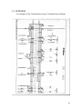
EXECUTIVE SUMMARY
This report summarizes research work conducted under TO4304 at the University of
California, Irvine. Under this task order, the research team provided Caltrans with on-call
direct support, technical guidance, and research related support. A series of Paramics
plug-ins were developed and have been released to Caltrans. These plug-ins include
actuated signal, multiple actuated signal timing plan, actuated signal coordination,
detector data aggregator, ramp metering control, on-ramp queue override control,
ALINEA ramp metering control, BOTTLENECK ramp metering control, SWARM
Ramp metering control, and Freeway MOE. They complement the current Paramics
simulation model and enhance its functionalities.
This report describes how we developed these plug-ins and the step-by-step procedure to
use them. It can be used as user manuals.
iii
Table of Contents
ACKNOWLEDGEMENTS................................................................................................ ii
EXECUTIVE SUMMARY ............................................................................................... iii
Table of Contents............................................................................................................... iv
1. Actuated signal Control .................................................................................................. 1
1.1 Introduction............................................................................................................... 1
1.2 Plugin implementation .............................................................................................. 1
1.3. Step-by-step user manual......................................................................................... 5
1.4. Working with different phasing sequences............................................................ 12
1.5 PROGRAMMER capabilities................................................................................. 21
1.6 Technical Supports.................................................................................................. 22
1.7 APPENDIX............................................................................................................. 24
2. Multiple Actuated Signal Plan ...................................................................................... 32
2.1. Introduction............................................................................................................ 32
2.2 Plug-in Implementation .......................................................................................... 32
2.3 Step-by-step user manual........................................................................................ 32
3. Actuated signal Coordination ....................................................................................... 35
3.1 Introduction............................................................................................................. 35
3.2 Plugin implementation ............................................................................................ 35
3.3 Step-by-step user manual........................................................................................ 37
4. Detector Data Aggregator ............................................................................................. 43
4.1 Introduction............................................................................................................. 43
4.2 Plugin implementation ............................................................................................ 44
4.3 Step-by-step user manual........................................................................................ 46
4.4. PROGRAMMER capabilities................................................................................ 49
5. Ramp metering control ................................................................................................. 51
5.1 Introduction............................................................................................................. 51
5.2 Plugin implementation ............................................................................................ 51
5.3 Step-by-step user manual........................................................................................ 55
5.4 PROGRAMMER capabilities................................................................................. 58
5.5 Technical Supports.................................................................................................. 59
6. On-ramp queue override control................................................................................... 61
6.1 Introduction............................................................................................................. 61
6.2 Plugin implementation ............................................................................................ 61
6.3 Step-by-step user manual........................................................................................ 62
6.4 Technical supports: References .............................................................................. 66
7. ALINEA ramp metering control................................................................................... 67
7.1. Introduction............................................................................................................ 67
7.2 Plugin implementation ............................................................................................ 68
7.3 Step-by-step user manual........................................................................................ 68
7.4 Technical Supports.................................................................................................. 72
8. BOTTLENECK ramp metering control........................................................................ 74
8.1 Introduction............................................................................................................. 74
8.2 Plugin implementation ............................................................................................ 75
iv
8.3 Step-by-step user manual........................................................................................ 76
8.4 Technical Supports.................................................................................................. 81
9. SWARM Ramp metering control ................................................................................. 83
9.1 Introduction............................................................................................................. 83
9.2 Plugin implementation ............................................................................................ 84
9.3 Step-by-step user manual........................................................................................ 87
9.4 Technical Supports.................................................................................................. 96
9.5 APPENDIX............................................................................................................. 98
10. Freeway MOE............................................................................................................. 99
10.1 Introduction........................................................................................................... 99
10.2 Step-by-step user manual...................................................................................... 99
10.3 PROGRAMMER capabilities............................................................................. 101
v
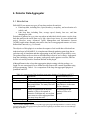
1. Actuated signal Control
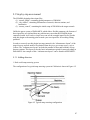
1.1 Introduction
Generally, modes of traffic signal operation can be divided into three primary categories
(USDOT, 1996): pre-timed, actuated and traffic responsive. PARAMICS can basically
model the fixed-time signal control. Besides, PARAMICS also provides a plan/phase
language (i.e. a kind of script language) to simulate some simple actuated signal control
logic. However, in the field the widely used actuated signal controller uses the complex
NEMA logic or type-170 logic. Our experiences found this script language is difficult to
be used to model these types of complex control schemes and to replicate these schemes
to multiple signalized intersections.
A plugin was developed in order to easily model actuated signal control within
PARAMICS. This report discusses the logic of this plugin as well as its implementation.
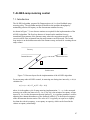
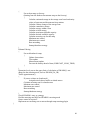
1.2 Plugin implementation
1.2.1 Control logic
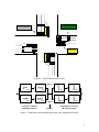
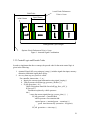
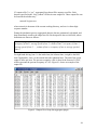
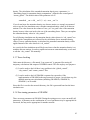
The layout of a typical actuated signal intersection is shown in Figure 1.1.
The control logic that is implemented in the plugin is for an eight-phase, dual-ring,
concurrent controller actuated signal. The dual-ring, concurrent concept is illustrated
briefly in Figure 1.2. Note that eight phases are shown, each of which accommodates one
of the through or left turning movements. A “barrier” separates the north-south phases
from the east-west phases. Any phase in the top group (Ring 1) may be displayed with
any phase in the bottom group (Ring 2) on the same side of the barriers without
introducing any traffic conflicts. For simplicity, the right turns are omitted and assumed
to proceed with the through movements.
In the fully-actuated signal control, all phases at an intersection are actuated. Therefore
the length of each phase, and consequently the cycle length, will vary with each cycle.
Some phases may be skipped if there is no vehicle actuation. To simulate the real
controller better, the order and sequence of phases can also be altered. The detailed
description on how actuated signal works can be found in the textbook by McShane et al
(1998).
1
Advance detector
Presence detector
Long loop
Figure 1.1 Typical Intersection Layout
Ring 1
W BL
EBL
Left side of barrier
(E-W Movem ents)
NBL
EBT
W BT
Ring 2
Barrier
SBL
SBT
NBT
Right Side of barrier
(N-S Movem ents)
Figure 1.2 Dual-ring concurrent phasing scheme with assigned movements
2
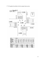
1.2.2 Modeling vehicle detection
The vehicle detection is an important part of the actuated signal system. There are three
groups of detectors in each approach for the typical intersection in the real world:
(1) Stopline detectors, located in the through lanes and very close to the stop line, for
the presence detection of through vehicles. There may be 2-3 presence detectors
for a lane that are typically about six feet by six feet in size;
(2) Advance loop detector, located at almost 150-300 feet from the stop bar, used to
detect vehicles for the extension of the through movement phase; and
(3) Long loop detector for left turns, with the length of about 50-70 feet, for the
presence detection of left turn vehicles. In some cases a set of individual detectors
are used instead of a single long one.
For some intersections, there may be no advance detector at some approaches of an
intersection. If presence detectors are only placed on the minor cross street, the signal has
semi-actuated control.
To better simulate the functionality of detectors, ideally detectors should be modeled in
PARAMICS according to the real-world configuration. However, in Build 3 of
PARAMICS, detectors are not lane specific. A detector covers all lanes of a link and thus
a PARAMICS detector represents a detector station. Therefore, we cannot model a
separate long loop (for left turn use) in the actuated signal system. As a result, we use
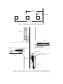
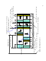
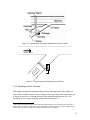
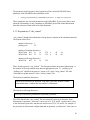
three small detectors instead of a long loop, as shown in Figure 1.3.
Three 2 m or 6.6 ft detectors are used to mimic one 50 ft long loop detector. These
detectors model the stopline presence detectors as well as the left-turn detectors. The
default length of detectors in PARAMICS is 2 meters, or 6.6 feet. The lengths of these
detectors in PARAMICS do not match the common real-world length of six feet, but for
the purposes of simulation this works fine.
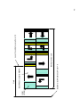
As illustrated in Figure 1.4, we modeled 16 detectors for a typical intersection in
PARAMICS and each detector covers all lanes of a link. For each approach, there are
three detectors close to the stop line for through and left-turn vehicle presence detection,
and one advance detector located at about 150-300 feet to the stop line for detecting
vehicles for the extension of the through movement phase. For stopline detectors, all
three of them employ the vehicle presence of left turn lanes; the two detectors close to the
stop line are used for detecting the presence of through vehicles.
Due to improvements in the long loop detection in later versions of PARAMICS (later
than Build V.3.0.7), we can use one long loop instead of three stopline loop detectors for
vehicle presence. As a result, we only need to model 8 detectors for an intersection. That
is to say, detectors 1, 5, 9 and 13 are long loops (with a typical length of 50 feet), and
there is no need to code detectors 2, 3, 6, 7, 10, 11, 14, and 15. This is our recommended
method to model detectors of an actuated signal intersection.
In version 4 of PARAMICS, detectors can be lane specific. This plugin does not support
the use of this type of detector.
3
31.2 ft
or 9.5 m
12.9 ft
or 4 m
Stop line
49.5 ft
or 15 m
Figure 1.3 Modeling the left turn long loop detector
8
Approach 2
7
6
5
Approach 1
4
1
7
2
3
4
6
1
5
2
12
11 10
3
9
8
NEMA Phase
Detector num ber
Approach 3
13
14
Detector
15
Approach 4
16
Figure 1.4 Typical Intersection Layout in PARAMICS with NEMA phases
4
1.2.3 Pseudo code
The pseudo code for the main control logic of this plugin is given as follows:
1. Initialize the actuated signal plugin, including signal data input, memory
allocation, and initial signal phase set up.
2. At every time step of simulation, net_action is called:
For controller intersection = 1 : n {
a. Inquiry the current signal information using signal_inquiry( ).
b. If ( left green time == 0 ) {
Amber and red time are counted.
If ( amber and red time are reached )
Set the next signal phase parameters through signal_action( ).
}
else {
vehicle presence detection (pp_presence_dection ( ) ).
excute the current signal plan (pp_excute_plan ( ) ) {
If ( left green time < extension &&
vehicle presence for extension &&
expired green < ( maximal green – extension ) ) {
green time increased by (extension – left green).
}
If ( left green time <= time step )
Find the next phase by vehicle presence
}
}
}
1.3. Step-by-step user manual
1.3.1 Data preparation
The data input to this plugin is the signal timing plan, the geometry and detector
information of actuated signal intersections.
If the purpose of simulation is to model a real-world network, the following information
is required in order to make actuated signals:
(1) Signal Timing Chart obtained from the proper government agency
(2) Geometric layout of the intersection; the best source of this information is usually
from as-built plans.
5
If the purpose of simulation is to evaluate an intersection design (or, test signal timing
plans), you can obtain the signal timing from traffic signal software, such as SYNCHRO,
based on historical traffic patterns.
1.3.2 Adding detectors and checking network coding
Based on the previous discussion, we can either code 16 detectors or 8 detectors to a fourlegged actuated signal intersection. The exact set-back distance of the advance detector
can found in the “Geometric layout of the intersection”.
The following geometric information needs to be checked:
(1) Number of lanes for each approach;
(2) Lane use information at intersections (for example, at an approach of an
intersection, which lanes are assigned to the left turn, through, or right turn
movements). If the default lane configuration is not the same as that shown in the
“Geometric layout of the intersection”, the corresponding intersection needs to be
re-coded via the PARMICS Modeller GUI (Node->Modify junction) or by editing
the “junctions” file manually.
1.3.3 Preparation of worksheet
Running MODELLER, zoom in to the intersection. Fill out a worksheet that includes
geometry and signal timing information of the intersection. The worksheet has been
attached in APPENDIX 1 of this document.
The following is a list of necessary information in the worksheet:
(1) Write down the name of the intersection, i.e. Alton & ICD, and the signal ID that
is shown in the first page of signal timing chart.
(2) Write down the two street names, the direction, and the PARAMICS designation
of the junction node and the four adjacent nodes on four approaches.
(3) Find NEMA movement number 1, generally a left turn, from the Signal Timing
Chart. Write down the turn arrow and the movement number 1. As a result, all
NEMA movements / phases can be determined based on the definition of the
standard NEMA phases / movements shown in figure 1. Write down all NEMA
movements on the worksheet.
(4) Write down the approach number on the worksheet. The approach that the 1st
NEMA movement locates is defined as approach 1 here. The counter-clockwise
approaches around the junction are defined as approach 2, 3, 4.;
6
(5) Fill out the 3-5 rows (Initial green, Extension, Max green) of the table on the
bottom of the worksheet. The ini_green corresponds to the “Initial”(green time)
and the max_green corresponds to the “Max Green” in the Signal Timing Chart.
(6) Find out the recall movement from “Signal Timing Chart”. Enter the two recall
movement numbers into the first two columns of the “recall” row. If there is only
one recall phase, put the second one as 0;
(7) Find out how many lanes correspond to each NEMA movement from “layout of
the intersection” or PARAMICS environment. Fill them in the row of “lanes” in
the worksheet. The first value in the row corresponds to the number of lanes for
NEMA movement 1 and the second value corresponds to NEMA movement 2, etc.
In many situations there are lanes that are shared by different movements. For
example, one lane may allow both left turning and through vehicles to pass. In
this case, the lane will count both as one through lane and as one half (0.5) of a
left-turning lane.
(8) From the layout, find out how many right turn lanes for each approach (1 -> 4).
Please refer to the definition at step 4 for the definition of approaches 1 to 4.
Write down these numbers in the row of “Right-turn lanes”. As in the case of
lanes that allow both left and through movements, lanes that allow through and
right-turn movements will count as one through lane and one half of a rightturning lane.
(9) The row of “detector 1’ to “detector 4” should be filled with the name of detectors
(the sequence is from stopline detectors to the advance detector, seen in figure 1)
on “approach 1” to “approach 4”. Please refer to the definition at step 4 for the
definition of approaches 1 to 4. In some cases, one or more of the detectors for an
approach does not need to be modeled. Each missing detector needs to be
specified as “N/A” in the worksheet. In Paramics v3.0 build 6, it was necessary to
place three separate detectors at the stopline to ensure proper detection. However,
build 7 of Paramics 3.0 and all later versions only need one long detector. To
allow reverse compatibility, it still might be desirable to place three separate
detectors.
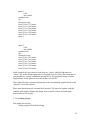
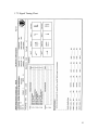
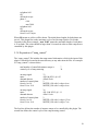
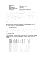
1.3.4 Preparation of “signal_control” file
The plugin requires a file titled “signal_control” to be in the PARAMICS network
directory. An example of the “signal_control” file is shown in Figure 1.5.
The first line of this file specifies the number of actuated signals modeled in the network.
The remainder of the file contains the signal timing information. The information in this
file has a very similar format to that of the worksheet. There are two signals modeled in
Figure 1.5. The first one uses 16 detectors and the second used 8 detectors.
7
Figure 1.5 An example of signal_control file
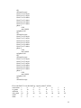
1.3.5 Preparation of “priorities” information
The “priorities” file defines what movement can be allowed under each phase of an
intersection. For pre-timed signal control, the priorities information can be edited through
the PARAMICS GUI. However, for the actuated signal, the file “priorities” must be
edited directly with a text editor.
We need to generate the “priorities” information of an actuated signalized intersection
based on the worksheet we made on step 2, in which the node names of adjacent nodes of
an intersection have been written down. Figure 1.6 is an example of the node
designations for a four-legged intersection. “approach 1” is considered to be in the
direction starting at node 7511 and heading towards the junction node 528z.
The “priorities” for a four-legged full-actuated intersection will have eight phases. As
illustrated in Figure 1.7, “Phase 1” will correspond to the situation where the left-turning
NEMA movements 1 and 5 will be given the green. “Phase 2” will account for the
situation where movements 5 and 2 will be given the green, and “phase 3” will be for
movements 1 and 6. “Phase 4” will be for the through movements 2 and 6. The last four
phases will follow the pattern of the first four phases, starting with the left-turn
movements 3 and 7.
8
7510
528z
7511
7614
7612
Figure 1.6 Intersection Layout
1+5
2+5
3+7
1+6
2+6
4+7
3+8
4+8
Figure 1.7 Eight phases of the four-legged full-actuated signal intersection
For the intersection in the previous figure, the definition of phases and actions
(movements) in “priorities” file would be:
actions 528z
phase offset 0.00 sec
phase 1
0.00
max 100.00
red phase 0.00
fill
all barred except
from 7510 to 7511 minor
from 7511 to 7612 minor
from 7511 to 7510 major
from 7612 to 7614 minor
from 7614 to 7612 major
from 7614 to 7510 minor
9
phase 2
0.00
max 100.00
red phase 0.00
fill
all barred except
from 7510 to 7511 minor
from 7511 to 7612 minor
from 7511 to 7614 major
from 7511 to 7510 major
from 7612 to 7614 minor
from 7614 to 7510 minor
phase 3
…
phase 8
0.00
max 100.00
red phase 0.00
fill
all barred except
from 7510 to 7511 minor
from 7510 to 7612 major
from 7511 to 7612 minor
from 7612 to 7614 minor
from 7612 to 7510 major
from 7614 to 7510 minor
In this example, the movements of each phase are “major” while all right turns are
“minor”. We set the default signal time of each phase as 0 sec (This is the reason that we
cannot edit these “actions” information through GUI). The plugin will assign a certain
length of time to each phase based on the presence of vehicles.
Then, update the above priorities information of the corresponding signalized node in the
“priorities” file of the network.
Please note that the network with modified “priorities” file must use together with this
actuated signal plugin. Without this plugin, all movements of those actuated signal
intersections are in red light.
1.3.6 Loading plugin
This plugin has two files:
actuated_signal.dll: Modeller Plugin
10
actuated_signal-p.dll: Processor Plugin
After the completion of the “signal_control” file and the update the “priorities” file, you
can load the simulation network together with this plugin.
PARAMICS introduces a network specified method to load plugins. Each network has a
“programming” file, which contains the plugins used together with the network. If you
put this plugin in the PARAMICS root directory (where you can find other Quadstone’s
plugins, including HOV, Loop aggregator, Monitor, etc.), you do not need to specify the
path of this plugin in the “programming” file:
actuated_signal.dll
If this plugin is stored to a directory other than the root directory of PARAMICS, the path
of the loaded plugin needs to be specified:
\Program Files\ParamicsV4\uci_plugins\actuated_signal.dll
Note PARAMICS thinks this plugin is in Drive C only. If you put this plugin to Driver D
or others, PARAMICS will not find the plugin. If you prefer to put this plugin to Driver
D or others, you have to use the way of version 3 of PARAMICS to load plugins.
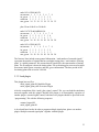
1.3.7 Error checking
After the network and the plugin are loaded in Modeller, you can start simulation. Via
GUI, you will see that this plugin emulates the actuated signal control at specified
intersections. This plugin can work if “signal_control” and “priorities” are prepared
correctly. If there is any mistake in the “signal_control” file, the plugin will be disabled.
The report window of PARAMICS will show whether this plugin works. This plugin
generates a file named “Log-signal.txt” under the network directory, which can be used to
check if the “signal_control” file has been understood by this plugin correctly.
The detector information in the “signal_control” file is connected with the “priorities”
information of the signal intersection. The mismatch of them may cause the signal work
abnormally. Two methods can be used to judge if the actuated signal control has the
correct logic:
(1) Based on the observation from GUI (Node->Modify junction->Signal display), or
(2) Making a long time simulation run and then check if there are any serious
congestion happened at actuated signal intersections. If an actuated signal control
is not working correctly, all input files need to be double checked for any
mistakes.
The correct use of this plugin depends on your knowledge of signal control. If necessary,
please have a look at related chapters in the textbooks.
11
1.3.8 Exercises
In APPENDIX (Section 1.7), 1.7.2 and 1.7.3 show the “Signal Timing Chart” and
“Geometric layout of the intersection ICD & BARRANCA”. Based on Section 1.2.2, we
filled in the worksheet, shown in 1.7.4. Based on this worksheet, the “signal_control”
information is shown in Section 1.3.4. Its “priorities” information is shown in 1.7.5.
This plugin can be used to model more complex actuated signal control through proper
configurations of the “priorities” and “signal_control” information. Users can learn more
from one of our example Irvine networks, which includes 37 actuated signals.
1.4. Working with different phasing sequences
In dual-ring operation, full-actuated signal controllers are capable of a number of phase
sequences between barriers. For each of the two major phase groups, there are three basic
phase sequences:
1. Left-turn first
2. Lead-leg left-turns, and
3. Through movement first
The developed full-actuated signal plugin can work with all three sequences. We have
described how to work with the “left-turn first” case in the previous section. This section
will discuss how to make the plugin to work under the second and third phase sequences.
Please refer to the example networks for further understanding this section.
1.4.1 Lead-leg left-turns
The layout of a typical intersection is as shown in Figure 1.8.
In the signal_control file, the two phases on the lead leg need to be put to the columns of
movement 1 and movement 5. If we want to make link 14:10 as the lead leg, the phase
sequence will be 2&5-> 1&5 -> 2&6 ->1&61, the corresponding signal_control file needs
to be configure as follows.
Movements
ini_green
extension
max_green
recall
lanes
rightturn
2
10
4
32
4
2
1
1
5
3
24
8
2
1
3
5
3
24
4
8
5
32
5
5
3
24
6
10
4
32
7
5
3
24
8
8
5
32
2
1
3
1
2
2
2
3
1
The real-world controller may not have the phase combination of 1 & 5. Our plugin cannot avoid having
it. But its existence does not have any negative (but positive) influence on the operation of the control logic.
12
detector1
detector2
detector3
detector4
icbsw
icbss
icbse
icbsn
N/A
N/A
N/A
N/A
N/A
N/A
N/A
N/A
icbuw
icbus
icbue
icbun
11
4 7
5
14
10
6
1
13
2
3 8
12
Figure 1.8 Phase layout of a signalized intersection
Based on phase sequences, 2&5 -> 1&5 -> 2&6 ->1&6, the priorities file needs to put
2&5 to phase 1, 1&5 to phase 2, 2&6 to phase 3 and 1& 6 to phase 4.
actions 10
phase offset 0.00 sec
phase 1
0.00
max 100.00
red phase 0.00
fill
all barred except
from 14 to 11 major
from 14 to 12 major
from 14 to 13 major
from 11 to 14 minor
from 13 to 11 minor
from 12 to 13 minor
phase 2
0.00
max 100.00
red phase 0.00
13
fill
all barred except
from 13 to 12 major
from 14 to 11 major
from 11 to 14 minor
from 13 to 11 minor
from 14 to 12 minor
from 12 to 13 minor
phase 3
0.00
max 100.00
red phase 0.00
fill
all barred except
from 13 to 14 major
from 13 to 11 major
from 14 to 13 major
from 14 to 12 major
from 11 to 14 minor
from 12 to 13 minor
phase 4
0.00
max 100.00
red phase 0.00
fill
all barred except
from 13 to 14 major
from 13 to 12 major
from 13 to 11 major
from 11 to 14 minor
from 14 to 12 minor
from 12 to 13 minor
phase 5
0.00
max 100.00
red phase 4.00
fill
all barred except
…
If we want link 13:10 as the lead leg, “signal_control” will be:
movements
ini_green
extension
max_green
recall
lanes
1
5
3
24
4
2
2
10
4
32
8
2
3
5
3
24
4
8
5
32
6
10
4
32
5
5
3
24
7
5
3
24
8
8
5
32
2
3
2
2
2
3
14
rightturn
detector1
detector2
detector3
detector4
1
icbsw
icbss
icbse
icbsn
1
N/A
N/A
N/A
N/A
1
N/A
N/A
N/A
N/A
1
icbuw
icbus
icbue
icbun
The corresponding proiorities file will not be listed here. Users can easily figure out.
1.4.2 Through movement first
Based on the description of the last section, we can deduce that the phase 2 and 6 should
be put to the location of the columns of movement 1 and movement 5.
As shown in the below figure, if we want phases 2 and 6 go first, the following phases
will be 2&6 -> 1&6 -> 2&5 -> 1&5. The signal_control file should be:
movements
ini_green
extension
max_green
recall
lanes
rightturn
detector1
detector2
detector3
detector4
2
10
4
32
4
2
1
icbsw
icbss
icbse
icbsn
1
5
3
24
8
2
1
N/A
N/A
N/A
N/A
3
5
3
24
4
8
5
32
6
10
4
32
5
5
3
24
7
5
3
24
8
8
5
32
2
1
N/A
N/A
N/A
N/A
3
1
icbuw
icbus
icbue
icbun
2
2
2
3
For the “priorities” file, we can just put 2&6, 1&6, 2&5, and 1&5 to the phase 1, 2, 3 and
4, as shown below.
actions 10
phase offset 0.00 sec
phase 1
0.00
max 100.00
red phase 0.00
fill
all barred except
from 13 to 11 major
from 13 to 14 major
from 14 to 12 major
from 14 to 13 major
from 11 to 14 minor
from 12 to 13 minor
phase 2
15
0.00
max 100.00
red phase 0.00
fill
all barred except
from 13 to 11 major
from 13 to 14 major
from 13 to 12 major
from 11 to 14 minor
from 14 to 12 minor
from 12 to 13 minor
phase 3
0.00
max 100.00
red phase 0.00
fill
all barred except
from 14 to 11 major
from 14 to 12 major
from 14 to 13 major
from 11 to 14 minor
from 13 to 11 minor
from 12 to 13 minor
phase 4
0.00
max 100.00
red phase 0.00
fill
all barred except
from 13 to 12 major
from 14 to 11 major
from 11 to 14 minor
from 13 to 11 minor
from 14 to 12 minor
from 12 to 13 minor
phase 5
0.00
max 100.00
red phase 4.00
fill
all barred except
…
1.4.3 Split phases
16
Except the above-mentioned cases, users may need to make signals work under split
phases. For example, there are only two possible phase combinations, 1&6 and 2&5, in
the first phase group. Under this situation, the signal timing chart from the local
transportation agency may provide phase information, which may not make this plugin
work as expected.
1.4.3.1 2&5 first and 1&6 second
The “signal_control” file can be configured as:
movements
ini_green
extension
max_green
recall
lanes
rightturn
detector1
detector2
detector3
detector4
2
10
4
32
4
5
0
icbsw
icbss
icbse
icbsn
1
5
3
24
8
5
1
N/A
N/A
N/A
N/A
3
5
3
24
4
8
5
32
9
0
0
0
9
0
0
0
7
5
3
24
8
8
5
32
2
0
N/A
N/A
N/A
N/A
3
1
icbuw
icbus
icbue
icbun
0
0
2
3
There is no phase 5 and 6. Only phases 1 and 2 exist. Note that movement (i.e. phase) 1
includes all lanes of link 13:10 and phase 2 includes all lanes of link 14:10 no matter the
lane is reserved for left turns or through movements. We can also configure the
“signal_control” file in another way, i.e. without phases 1 and 2 but with phases 5 and 6,
as shown below. The previous phase 1 goes to phase 6 and the previous phase 2 goes to
phase 5.
movements
ini_green
extension
max_green
recall
lanes
rightturn
detector1
detector2
detector3
detector4
9
0
0
0
4
0
0
icbsw
icbss
icbse
icbsn
9
0
0
0
8
0
1
N/A
N/A
N/A
N/A
3
5
3
24
4
8
5
32
5
10
4
32
6
5
3
24
7
5
3
24
8
8
5
32
2
0
N/A
N/A
N/A
N/A
3
1
icbuw
icbus
icbue
icbun
5
5
2
3
For the “priorities” file, phase 1, 2 and 3 have the same allowed movements.
actions 10
phase offset 0.00 sec
phase 1
0.00
17
max 100.00
red phase 0.00
fill
all barred except
from 14 to 11 major
from 14 to 12 major
from 14 to 13 major
from 11 to 14 minor
from 13 to 11 minor
from 12 to 13 minor
phase 2
0.00
max 100.00
red phase 0.00
fill
all barred except
from 14 to 11 major
from 14 to 12 major
from 14 to 13 major
from 11 to 14 minor
from 13 to 11 minor
from 12 to 13 minor
phase 3
0.00
max 100.00
red phase 0.00
fill
all barred except
from 14 to 11 major
from 14 to 12 major
from 14 to 13 major
from 11 to 14 minor
from 13 to 11 minor
from 12 to 13 minor
phase 4
0.00
max 100.00
red phase 0.00
fill
all barred except
from 13 to 14 major
from 13 to 12 major
from 13 to 11 major
from 11 to 14 minor
from 14 to 12 minor
from 12 to 13 minor
18
phase 5
0.00
max 100.00
red phase 0.00
fill
all barred except
…
1.4.3.2 1&6 first and 2&5 second
The “signal_control” file needs to be one of the following two:
movements
ini_green
extension
max_green
recall
lanes
rightturn
detector1
detector2
detector3
detector4
1
5
3
24
4
5
0
icbsw
icbss
icbse
icbsn
2
10
4
32
8
5
1
N/A
N/A
N/A
N/A
movements
ini_green
extension
max_green
recall
lanes
rightturn
detector1
detector2
detector3
detector4
9
0
0
0
4
0
0
icbsw
icbss
icbse
icbsn
9
0
0
0
8
0
1
N/A
N/A
N/A
N/A
3
5
3
24
4
8
5
32
9
0
0
0
9
0
0
0
7
5
3
24
8
8
5
32
2
0
N/A
N/A
N/A
N/A
3
1
icbuw
icbus
icbue
icbun
0
0
2
3
3
5
3
24
4
8
5
32
6
5
3
24
5
10
4
32
7
5
3
24
8
8
5
32
2
0
N/A
N/A
N/A
N/A
3
1
icbuw
icbus
icbue
icbun
4
5
2
3
The corresponding “priorities” file is:
actions 10
phase offset 0.00 sec
phase 1
0.00
max 100.00
red phase 0.00
fill
all barred except
from 13 to 14 major
19
from 13 to 12 major
from 13 to 11 major
from 11 to 14 minor
from 14 to 12 minor
from 12 to 13 minor
phase 2
0.00
max 100.00
red phase 0.00
fill
all barred except
from 13 to 14 major
from 13 to 12 major
from 13 to 11 major
from 11 to 14 minor
from 14 to 12 minor
from 12 to 13 minor
phase 3
0.00
max 100.00
red phase 0.00
fill
all barred except
from 13 to 14 major
from 13 to 12 major
from 13 to 11 major
from 11 to 14 minor
from 14 to 12 minor
from 12 to 13 minor
phase 4
0.00
max 100.00
red phase 0.00
fill
all barred except
from 14 to 11 major
from 14 to 12 major
from 14 to 13 major
from 11 to 14 minor
from 13 to 11 minor
from 12 to 13 minor
phase 5
0.00
max 100.00
red phase 0.00
fill
20
all barred except
…
1.5 PROGRAMMER capabilities
1.5.1 Interface functions
Interface functions have been provided by this plugin for external modules to acquire and
change the default timing plan. This plugin provided a couple of interface functions for
external plugin modules to acquire the current signal timing plan and set a new timing
plan to a specific signal. An advanced signal control algorithm plugin can be further
developed based on them. The prototypes of these interface functions are shown below.
Signal* uci_signal_get_parameters(char *nodeName);
Function:
Querying the current signal timing plan of a specific actuated signal
Return Value: The current timing plan of an actuated signal.
Parameters: nodeName is the name of the signal node.
Signal is the structure of actuated signal data, whose definition is:
type Signal
{
// intersection name and location
char *node;
char *controllerLocation;
// signal parameters
int movements[8];
float maximumGreen[8];
float minimumGreen[8];
float extension[8];
float storedRed[8];
float phaseGreenTime[8];
float movementGreenTime[8];
// current phase information
int currentPhase;
int expiredTime;
float redTimeLeft;
Bool cycleEndFlag;
}
Void uci_signal_set_parameters(Signal *sig);
Function:
Setting a new timing plan to a specific signal.
Return Value: None
21
Parameters:
sig stores the new timing plan.
1.5.2 How to use interface functions in other plugins
These two interface functions can be called in other plugins. The following setting is
required:
(1) In the workspace of your plugin that wants to use these interface functions,
specify the library file “actuated_signal.lib” of the actuated signal plugin as an
input object/library module. The path of “actuated_signal.lib” should be specified
as well.
(2) Specify the prototype of the interface function at the beginning of your plugin as
follows:
_declspec(dllimport) void uci_signal_set_parameters(Signal *sig);
_declspec(dllimport) Signal* uci_signal_get_parameters(char *nodeName);
1.6 Technical Supports
1.6.1 Limitations of this plugin
1) During our development on this full-actuated signal control plugin, we found that
PARAMICS did not provide a plugin function for users to control the amber time (yellow
light). Although yellow time can be set in the configuration file, it is a universal
parameter for all the intersections and all the time. It is not convenient in the actuated
signal case since some phases may be skipped (the amber time has to be skipped at the
same time). In order to simulate the real world better, our developed plugins have to have
a handle on the control of the amber time associated with each phase.
2) In PARAMICS, phase and movement are different. For the current actuated signal
plugin implementation, each phase usually includes two major movements, and some
minor movements. For instance, phase 1 may include dual left turn movements, and some
right turn minor movements. PARAMICS runs through phase 1 to phase 8, some phases
may be skipped depending on the vehicle presence. However, each movement has its own
initial green and extension in the signal-timing sheet. Only one set of parameters could7 be
used in each phase. Although a reasonable set of parameters is calculated and used during
the simulation, and doing this does not hurt the simulation performance, the actual signal
control cannot be fully simulated in this plugin. Ideally, we want each phase to include
only one major movement, and two phases can be executed at the same time. Version 4
of PARAMICS provides users with this capability but we do not have time to implement
this at the current time.
3) Only one timing plan for each intersection is supported by the current plugin. In order
to support multiple signal plans, please use another plugin “multiple actuated signal plan”
together with this plugin.
22
4) In version 3 of PARAMICS, vehicles may stop at stop lines because of routing
problem (such as a through vehicle stopping on a left turn lane). Version 4 has bot this
problem because it introduces the re-routing feature.
1.6.2 FAQ:
1. Grammar of input files
Unlike the parser system of PARAMICS, which allow flexible grammars and comments
(i.e. ##), the format of the input file of this plugin is rigid and thus any problem in the file
may cause the plugin not work well. Our recommendation for users is that the input file
of the example network of this plugin is a good starting point to make your own input file
in order to avoid editing problems.
2. Can a phase in priorities file have no movement information?
It is not good for a phase to have no movement information. Every phase corresponds to a
combination of NEMA phases, if that phase is regarded to have vehicles and then a green
signal will be given to that phase, which has no movement allowed. Then, the plugin may
be locked to that phase. The solution is that you can repeat the movement information of
a related phase. Please refer to Section 1.4.3.
1.6.3 Tools
In order to speed up the process of coding actuated signals, we also make two computer
programs for the making of “signal_control” file and the “priorities” information. You
can request these tools from California ATMS testbed.
1.6.4 References
1. W.R. McShane, R.P. Roess and E.E. Prassas (1998). Traffic Engineering (Second
Edition). Prentice-Hall.
2. Liu, X., Chu, L., and Recker, W. (2001) “Paramics API Design Document for
Actuated Signal, Signal Coordination and Ramp Control”, California PATH
Working Paper, UCB-ITS-PWP-2001-11, University of California at Berkeley.
3. USDOT, Federal Highway Administration (1996) Traffic Control Systems
Handbook.
23
1.7 APPENDIX
1.7.1 Worksheet
_______ Dr
Location____________
Signal ID___________
(approach___)
Node ___
Direction
(approach__)
Node ___
Node ___
Node ___
(approach___)
(approach__)
________ Dr
Node ___
Node
Movement
Initial Green
Extension
Max Green
Recall Phase
Lanes
1
2
3
4
5
6
7
8
Right-Turn lanes
Detector 1
Detector 2
Detector 3
Detector 4
24
1.7.2 Signal Timing Chart
25
26
1.7.3 Geometric layout of the intersection
27
1.7.4 Completed worksheet for the example intersection
28
1.7.5 The priorities information for the example intersection
actions 1167
phase offset 0.00 sec
phase 1
0.00
max 100.00
red phase 0.00
fill
all barred except
from 1416 to 299 minor
from 1610 to 1416 minor
from 1610 to 1533 major
from 299 to 1416 major
from 299 to 1533 minor
from 1533 to 1610 minor
phase 2
0.00
max 100.00
red phase 0.00
fill
all barred except
from 1416 to 299 minor
from 1610 to 1416 minor
from 299 to 1416 major
from 299 to 1533 minor
from 299 to 1610 major
from 1533 to 1610 minor
phase 3
0.00
max 100.00
red phase 0.00
fill
all barred except
from 1416 to 299 minor
from 1610 to 1416 minor
from 1610 to 299 major
from 1610 to 1533 major
from 299 to 1533 minor
from 1533 to 1610 minor
phase 4
0.00
max 100.00
red phase 0.00
fill
29
all barred except
from 1416 to 299 minor
from 1610 to 1416 minor
from 1610 to 299 major
from 299 to 1533 minor
from 299 to 1610 major
from 1533 to 1610 minor
phase 5
0.00
max 100.00
red phase 0.00
fill
all barred except
from 1416 to 299 minor
from 1416 to 1610 major
from 1610 to 1416 minor
from 299 to 1533 minor
from 1533 to 299 major
from 1533 to 1610 minor
phase 6
0.00
max 100.00
red phase 0.00
fill
all barred except
from 1416 to 299 minor
from 1416 to 1533 major
from 1416 to 1610 major
from 1610 to 1416 minor
from 299 to 1533 minor
from 1533 to 1610 minor
phase 7
0.00
max 100.00
red phase 0.00
fill
all barred except
from 1416 to 299 minor
from 1610 to 1416 minor
from 299 to 1533 minor
from 1533 to 1416 major
from 1533 to 299 major
from 1533 to 1610 minor
phase 8
0.00
max 100.00
30
red phase 0.00
fill
all barred except
from 1416 to 299 minor
from 1416 to 1533 major
from 1610 to 1416 minor
from 299 to 1533 minor
from 1533 to 1416 major
from 1533 to 1610 minor
31
2. Multiple Actuated Signal Plan
2.1. Introduction
The actuated signal plug-in only supports one timing plan for each actuated signal. In
order to allow multiple signal timing plans, this plug-in can be used.
2.2 Plug-in Implementation
This plug-in is developed based on actuated signal plug-in. The pseudo code for the main
control logic of this plugin is given as follows:
1. Read the “multi_plan_signal_control” file and initialize the multiple actuated
signal plugin.
2. At every time step of simulation:
For controller intersection = 1 : n
{
If (time to switch timing plan)
{
Update signal timing plan using uci_signal_set_parameters().
}
}
2.3 Step-by-step user manual
2.3.1 Preparation of “multi_plan_signal_control” file
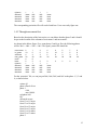
In order to use this plug-in, the input file of the plug-in: “multi_plan_signal_control”
needs to be prepared first. An example of this file is:
total number of actuated signals 2
total number of timing plans 2
plan 1 from 8:00:00 to 9:00:00
node 1167 ICD & BARRANCA
movements 1 2 3 4 5 6 7 8
ini_green 5 5 5 8 5 5 5 8
extension 3 4 3 5 3 4 3 5
max_green 24 32 24 32 24 32 24 32
32
node 142 ALTON & ICD
movements 1 2 3 4 5 6 7 8
ini_green 5 5 5 5 5 5 5 5
extension 3 5 3 5 3 5 3 5
max_green 24 32 24 32 24 32 24 32
plan 2 from 9:00:00 to 24:00:00
node 1167 ICD & BARRANCA
movements 1 2 3 4 5 6 7 8
ini_green 5 5 5 8 5 5 5 8
extension 3 4 3 5 3 4 3 5
max_green 20 28 20 28 20 28 20 28
node 142 ALTON & ICD
movements 1 2 3 4 5 6 7 8
ini_green 5 5 5 5 5 5 5 5
extension 3 5 3 5 3 5 3 5
max_green 20 28 20 28 20 28 20 28
The first two lines include some general information. “total number of actuated signals”
represents the number of signals that have multiple timing plans. “total number of timing
plans” is a global parameter. We assume that all signals have the same number of timing
plans. The second part is about the timing plans. For each timing plan, users need to input
movement, initial green, extension, and max_green information. The time period of the
last timing plan needs to end at 24:00:00.
2.3.2 Load plugin
This plugin has two files:
multi_signal_plan.dll: Modeller Plugin
multi_signal_plan-p.dll: Processor Plugin
After the completion of the “multi_plan_signal_control” file, you can load the simulation
network together with this plugin. Because this plugin is an functionality extension of
another plugin: actuated signal control, both these two plugins should be specified in the
“programming” file with the following sequence:
actuated_signal.dll
multi_signal_plan.dll
is developed based on the In order to support multiple signal plans, please use another
plugin “multiple actuated signal plan” together with this plugin.
33
2.3.3 Error checking
If any mistakes occurred in the “multi_plan_signal_control” file, this plugin will be
disabled. The report window of PARAMICS will show whether this plugin is working.
34
3. Actuated signal Coordination
3.1 Introduction
Coordination is a mode of signal operation designed to allow platoons of traffic to form
and "progress" through several signals with minimum stops and delay. Where signals are
closely spaced and traffic volumes are high, coordination of signals is necessary to avoid
excessive delay and stops.
The actuated signal coordination API inherits most parts of full-actuated signal API, with
additional force-off logic to maintain the background cycle length, and form green band
for a particular phase (sync phase).
3.2 Plugin implementation
3.2.1 Control logic
To provide synchronization and maintain the background cycle length, all coordinated
intersection have the same system clock reference point, which is usually the start point
of signal coordination plan. For the fixed-time signal coordination plan, there is an offset,
which is the difference between two green initiations of the sync phase for two adjacent
intersections. However, for the traffic-actuated signal coordination, the sync phase of
every coordinated intersection has fixed series of yield points, and the difference between
yield points is the background cycle length. These yield points are also local clock
reference points to other non-sync phases. The sync phase has minimal bandwidth, i.e.
the sync phase has to start at the time of minimal bandwidth earlier than yield point. To
do so, all other phases have to be cut at certain points, which are so-called force-off
points. These force-off points are usually referenced to the local clock reference point.
Figure 1 is the phase diagram of coordinated intersection.
35
Local Clock Reference
Point = 0 sec
Yield Point
Initial Green
Sync Phase
Background Cycle Length
System Clock Reference Point = 0 sec
Figure 1. Actuated Signal Coordination
3.2.2 Control Logic and Pseudo Codes
In order to implement the above concept, the pseudo code for the main control logic is
given in the following:
1. Actuated Signal API set up using api_setup( ), includes signal data input, memory
allocation, and initial signal phase set up.
2. At every time step, net_action is called:
For controller intersection = 1 : n {
a. Inquiry the current signal information using signal_inquiry( ).
b. Vehicle presence detection (pp_presence_dection ( ) ).
c. If (left green time > 0) {
Check if this phase should be forced off (pp_force_off ( )).
If (force-off )
Find the next phase by vehicle presence.
else {
excute the current signal plan (pp_excute_plan ( ) ) {
If ( left green time < extension &&
vehicle presence for extension &&
expired green < ( maximal green – extension ) ) {
green time increased by (extension – left green).
}
If ( left green time <= time step ) {
36
Find the next phase by vehicle presence.
}
}
}
}
else {
Amber and red time are counted.
If ( amber and red time are reached )
Set the next signal phase parameters through signal_action( ).
}
}
3.3 Step-by-step user manual
3.3.1 Understanding actuated signal coordination
The implemented actuated signal coordination logic has some new concepts. The correct
understanding of them is important for the use of the actuated signal coordination plugin.
The following is a good description of these terms:
1. Background Cycle Length
To provide synchronization and maintain the background cycle length, all coordinated
intersection have the same system clock reference point, which is usually the start point
of signal coordination plan.
2. Yield Point
The sync phase of every coordinated intersection has fixed series of yield points, and the
difference between yield points is the background cycle length.
3. Sync Phase
These yield points are also local clock reference points to other non-sync phases. The
sync phase has minimal bandwidth, i.e. the sync phase has to start at the time of minimal
bandwidth earlier than yield point.
4. Force Off
To do so, all other phases have to be cut at certain points, which are so-called force-off
points. These force-off points are usually referenced to the local clock reference point.
3.3.2 Data requirement
37
As the actuated signal API, two files need to be prepared for the use of signal
coordination API. One is the “priorities” file, provided by Paramics, to be used to identify
the hierarchy of movements for all phases. The other is the so-called
“signal_coordination_control” file, which contains all the signal timing information,
intersection layout information, and coordination information.
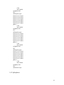
The following is an example of the part of “signal_coordination_control” file for one
intersection.
total number of actuated signals is:
node 6 ALTON & ICD
movements
1
2
3
4
ini_green
5
5
5
5
extension
3
5
3
5
max_green
24
60
24
32
recall
2
6
lanes
2
3
2
3
rightturn
1
1
1
1
detector1
aisw
ai2w ai3w
detector2
aiss
ai2s ai3s
detector3
aise
ai2e ai3e
detector4
aisn
ai2n ai3n
sync_phase
2
6
cycle_length 60
force_off
36
60
18
27
yield_point
5
system_clock 0
4
5
5
3
24
6
5
5
32
7
5
3
24
8
5
5
32
2
3
2
3
60
18
27
aiuw
aius
aiue
aiun
36
The data for signal coordination has been attached after the intersection layout data for
each intersection. Besides to the yield point of the sync phase, all other phases have
force-off points, referenced to the local clock reference point. Notice that the maximal
green time of primary sync phase has to be the cycle length, since the green time of sync
phase may occupy the entire cycle if there is no conflict traffic.
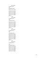
3.3.3 Example
38
Phase Interval Times
Interval
Phase
1
2
6
2.0
20
3
14
3.0
50
5
Red
1
1
1
Permit
√
√
√
Walk
Ped Clear
Initial
Extension
Max Green
Yellow
3
4
5
6
7
8
9
2.0
20
3
10
3.0
50
5
6
3.0
15
3
10
2.0
35
4
1
1
1
1
1
√
√
√
√
√
6
8
3.0 2.0
15 35
3
4
Max Recall
Min Recall
Ped Recall
Lag Phase
√
39
Local Clock Reference Point = 0
Background Cycle
System Clock Reference Point = 0
Initial
(Minimum)
Sync Phase (usually NEMA
Yield
40
4
10
6 6
4 6
Background Cycle Length = 120
6 6
4 10
4 8
5
5
F.O. 3 < 120 - 4 - 8 - 5 - 48 = 55 sec
F.O. 4 < 120 - 5 - 48 = 67 sec
F.O. 1 < 120 - 4 - 6 - 4 - 8 - 5 - 48 = 45 sec
Local Clock Reference Point = 0
System Clock Reference Point = 0
F.O. 8 = F.O. 4 < 120 - 5 - 48 = 67 sec
F.O. 6 = F.O.7 - 12 = 53 – 12 = 41 sec
F.O. 7 < F.O. 8 - 10 - 4 = 67 - 14 = 53 sec
F.O. 5 = F.O. 6 - 40 sec -4 sec
= 41 – 44 = -3 = 117 sec
9
NEMA 6 Bandwidth = 40
14
NEMA 2 Bandwidth = 48
Yield Point = 70
Check barrier: F.O. 1 < F.O.6 + 2 = 43 sec
41
21
4
40
6 6
4 6
6
10
Background Cycle Length = 120
10
6 6
13
4 10
4 8
F.O. 8 = F.O. 4 = 67 sec
34
5
5
System Clock Reference Point = 0
Hypothetical
42
F.O. 3 (< 55 sec) = 67 - 30 - 4 = 33 sec
30
F.O. 4 (< 67 sec) = 67 sec
F.O. 1 (< 43 sec) = 33 - 10 - 4 = 19 sec
Local Clock Reference Point = 0
F.O. 7 (< F.O. 8 - 14 sec) = 67 - 34 - 4 = 29 sec
F.O. 6 = F.O. 1 - 2 sec = 17 sec
F.O. 5 = F.O. 6 - 40 sec -4 sec
= 17 - 40 - 4 = - 27 sec
= 120 - 27 = 93 sec
9
NEMA 6 Bandwidth = 40
14
NEMA 2 Bandwidth = 48
Yield Point = 70
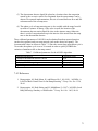
4. Detector Data Aggregator
4.1 Introduction
PARAMICS can output two types of loop detector data for analysis:
• Point loop data, including flow, speed, headway, occupancy, and acceleration of a
vehicle, and
• Link loop data, including flow, average speed, density, lane use, and lane
changing on a link.
Point data is gathered at every time step when an individual vehicle passes over the loop;
link data analyses the traffic data over a link, where loops locate, at a user-defined time
period. However, many Advanced Traffic Management and Information Systems
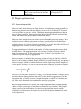
(ATMIS) applications demand point traffic data, but in an aggregated manner over userdefined time intervals, e.g. 30 seconds.
The objective of this plugin is to emulate the outputs of real-world data collection from
induction loops in PARAMICS. It is implemented through gathering point loop data at
each time step of simulation and then aggregating at any time interval specified by users.
The gathered data can be raw data or smoothed data in term of user’s choice. Aggregated
loop data (including volume, occupancy, and speed) can be output to text files, and can
be also accessed by interface functions defined in this plugin2.
Although Paramics has a loop data aggregation plugin coming with the package, we
found it is not convenient for us to further develop some traffic control algorithms using
APPI programming. Table 4.1 is a comparison of the loop data aggregator plugins of
Quadstone and UCI.
Table 4.1 comparison of the loop data aggregator plugins of Quadstone and UCI
Quadstone
ATMS testbed @ UCI
Measurements
flow, count, speed, gap, occupancy
count, occupancy, speed
Occupancy output Time occupancy
Percent occupancy
Grouped data and laneOutput files
A file only includes a lane’s data, or
the grouped data. Too many files will based data are in the same
file for a detector
be opened.
No restriction on the
Restriction
There are restrictions on the total
number of files to be
number of files to be opened in
Paramics. Problems may occur when opened
users want to collect aggregated data
for many loop detectors.
Programming
Programmer users can use data in the Full supports of advanced
2
There is another MYSQL version of Loop Data Aggregator plugin. MYSQL database is used for storing
aggregated loop data. All aggregated loop data since the beginning of simulation can be accessed through
querying the database.
43
capability
output files through reading them.
But, it is not convenient for on-line
applications.
algorithm plug-ins
developed by UCI
4.2 Plugin implementation
4.2.1 Aggregation method
In the real world, most detectors are loop detectors. A loop detector station generally has
multiple loop detectors and each loop detector covers a lane. In PARAMICS, a detector
can cover all lanes or just cover a lane. This plugin outputs aggregated detector data in
term of a detector station. The aggregated data outputs include not only aggregated data
of each lane but also the grouped data of the detector station.
In the real world, loop detectors are used to report volume and percent occupancy. In the
simulation, besides volume and percent occupancy, speed can also be obtained from
simulation because it is a basic element of simulation. As a result, this plugin will be used
to aggregate traffic volume, percent occupancy and speed data.
The aggregated volume is defined as the number of vehicles passing the detector during
last time interval. The aggregated speed is the average of speeds of passing vehicles
during last time interval. If at the aggregation time, a vehicle is just on a loop, it is
counted as a passed vehicle for aggregation.
Percent occupancy is defined as the percentage of time of a loop occupied by vehicles.
However, the occupancy obtained from PARAMICS (via API function loop_occupancy())
is time occupancy, which is calculated based on vehicle length, loop detector length, and
vehicle speed. Therefore, we need to convert from time occupancy to percent occupancy:
N
OCC =
∑OCC (i)
TT
i =1
where OCC(i) is the time occupancy of vehicle i; N is the total number of vehicles having
passed the detector during last time interval; TT is the interval of aggregation. If at the
aggregation time, a vehicle is just on a loop, the duration the vehicle is on the detector
(this value can be obtained from simulation) is used for aggregation.
Based on aggregated data of each lane, the grouped aggregated data (including grouped
volume, occupancy and speed) of this detector station are also calculated. The grouped
volume represents the total number of vehicles having passed the detector station
(including several detectors, each lane has one detector) during last time interval, which
can be expressed as
44
n
N i (t ) = ∑ N i , j (t )
j =1
where i is the index of the detector station; j is the loop index at detector station i; n is the
total number of lanes, or loops at detector station i; Ni,j(t) is the number of vehicles
passing loop j of detector station i during time interval (t-1, t).
The grouped occupancy represents the average percent occupancy of a detector station
during last time interval, which can be expressed as
Oi (t ) = (
1 n
∑
n j =1
Ni , j (t )
∑ (TO
k =1
(t ))) / TT
i , j ,k
where i is the index of the detector station; j is the loop index at detector station i; n is the
total number of lanes, or loops at detector station i; k is the vehicle index; Ni,j(t) is the
number of vehicles passing loop j of detector station i during time interval (t-1, t); TOi,j,k(t)
is the time occupancy of vehicle k passing loop j at detector station i during time interval
(t-1, t).
The grouped speed represents the average speed of a detector station during last time
interval, which can be expressed as
Vi (t ) =
1 1 n
(
∑
n N i (t ) j =1
Ni , j (t )
∑V
k =1
i , j .k
(t ))
where i is the index of the detector station; j is the loop index at detector station i; n is the
total number of lanes, or loops at detector station i; k is the vehicle index; Ni,j(t) is the
number of vehicles passing loop j of detector station i during time interval (t-1, t); Vi,j,k(t)
is the loop speed when vehicle k passes loop j at detector station i during time interval (t1, t).
4.2.2 Pseudo code
The control logic is given in the following pseudo codes:
1. Initialization of loop data aggregator plugin, including reading “loop_control” file,
opening output files, memory allocation, and other initial settings;
2. At every time step, PARAMICS overload API function:
“vehicle_detector()”when a vehicle traverses on or passes a loop. If a vehicle
passed a detector, the occupancy and speed of the vehicle are accumulated. The
following exceptional cases need to be handled in order to obtain the correct
occupancy value:
(1) Unexpected incorrect value of occupancy from simulation, which may happen
when a loop is placed at a location near the start or the end of a link;
(2) More than one vehicle are on a loop at the same time;
45
(3) One vehicle stays over a loop for more than certain time period, which may
happen when an incident or congestion appears;
(4) One vehicle is just on a loop at the time of aggregation.
3. At every time step, PARAMICS overload API function: “net_action()”.
For detector = 1:n
{
If it is the time to calculate and report the aggregated data of a loop
{
Calculate count, average speed, and percent occupancy of a detector.
Calculate grouped count, occupancy, and speed of all detectors at a
detector station
Output these data to output files and the interface function
}
}
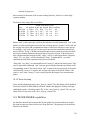
4.3 Step-by-step user manual
4.3.1 Preparation of the “loop_control” file
“loop_control” is the input file of the loop data aggregator plugin. This file should be put
to the same directory as any other network files. An example of “loop_control” file is
shown as follows:
detector count
report cycle
activation time
deactivation time
gather smoothed data
output to files
42
30
06:00:00
10:00:00
no
yes
name 405n0.6ml
gather interval 00:00:30
name 405n0.93fr
gather interval 00:00:60
…
There are two parts in the file. The first part is the general information about data
aggregation.
1. The first row of the file shows the number of detectors that are required to do the
aggregation operation.
46
2. The second row specifies the polling / report cycle of data aggregation. The unit is
seconds. This cycle is corresponding to the time interval of real-world loop data
collection. A typical value of the “report cycle” is 30 seconds. Basically, this
polling cycle is not related to aggregated data outputs. It is used for ATMS
applications, such as adaptive ramp metering, that are based on aggregated loop
data.
3. The next two rows specify the activation time and deactivation time of the loop
data aggregation.
4. The fifth row specifies whether to gather smoothed loop data (including speed,
occupancy). If “no”, raw data will be gathered. There are two kinds of loop data
that can be provided by PARAMICS at each time step, raw data or smoothed data.
Smoothed refers to a value tNs at time-step N smoothed using the expression:
t Ns = (1 − p)t Ns −1 + pt N
where tN is the current value and p is the co-efficient of smoothing.
5. The sixth row specifies whether to output aggregated loop data to files. If say
“yes”, a file, generally named as “XYZ.txt” (“XYZ” is the name of the
corresponding loop), will be generated for storing the aggregated volume,
occupancy and speed data based on the gather interval specified in the second part
of this control file.
The second part of the file contains the information of each loop detector, including the
name of detector and the time interval that loop data are aggregated and reported to text
files. There is a blank row between the information of any two loops. The name of a loop
can be found in the “detectors” file, which is one of network files. The time interval to
aggregate loop data can be different for different detectors.
4.3.2 Loading plugin
This plugin has two files:
loop_agg.dll: Modeller Plugin
loop_agg-p.dll: Processor Plugin
After the completion of the “loop_control” file, you can load the simulation network
together with this plugin. Run simulation and then you will obtain the aggregated loop
data outputs if you enable the option “output to files”.
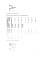
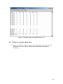
4.3.3 Text file outputs
47
If “output to files” is “yes”, aggregated loop data will be output to text files. Each
detector specified in the “loop_control” file has its own output file. These output files can
be found in the subdirectory:
network/Log/run-xxx
where network is the name of the current working directory, and xxx is a three-digit
sequence number.
During the simulation process, aggregated detector data are continuously calculated, and
then immediately stored to the output text file. Each output file has several fields, whose
definitions are shown as follows:
Time stamp, grouped volume, grouped occupancy, grouped speed, volume of lane 1,
occupancy of lane 1, average speed of lane 1, volume of lane 2, occupancy of lane 2,
average speed of lane 2, …, volume of lane n, occupancy of lane n, average speed of
lane n
For right hand driving, lane 1 is the inside lane (the leftmost lane, it might be the HOV
lane if applicable). Lane n is the outside lane (the rightmost lane). The unit of the speed
output is miles per hour. The percent occupancy value is show in the format of “0.094”,
which represents the percent occupancy of 9.4%. Figure 4.1 shows an example of the
output file.
Figure 4.1 Output file of loop data aggregator plugin
48
4.3.4 Error checking
This plugin is easy to use if “loop_control” is prepared correctly. If any mistakes
happened in the “loop_control” file, the plugin will be disabled. The report window of
PARAMICS will show whether this plugin is working.
If the plugin is not working, you may need to check if there is any error in “loop_control”.
This plugin generates a file named “Log-loop.txt” under the network directory, which can
be used to check if the “loop_control” file has been understood by this plugin correctly.
4.4. PROGRAMMER capabilities
4.4.1 Interface functions
This plugin provides three interface functions. The first one is used to obtain the current
polling / report cycle of data aggregation, defined in the second row of “loop_control”. If
an ATMS application, such as an adaptive ramp metering control, is based on aggregated
loop data, this interface can provide the polling cycle of aggregated loop data.
int uci_loop_agg_interval(void)
Return Value: The polling cycle of aggregated loop data.
Parameters: None
The second interface function is used to tell users if a loop detector has been specified in
“loop_control” file for getting aggregated loop data.
Bool uci_loop_aggregation(char *name)
Return Value: If the name of a loop detector has been specified in “loop_control” file,
return “TRUE”. Otherwise, return “FALSE”.
Parameters: Name of the loop detector.
The third interface function is used for querying the aggregated loop data of the latest
time interval at a detector station. The aggregated loop data includes grouped volume,
average occupancy and average speed, and lane-based volume, average occupancy and
average speed.
LOOPAGG uci_loop_agg (int index)
Return Value: The aggregated detector data of a loop detector
Parameters: index: the network-wide index number for a loop detector
LOOPAGG is a structure that has the following definition:
typedef struct loopagg LOOPAGG;
struct loopagg
{
int
index;
float time;
49
int
float
float
int
int
float
float
g_vol;
g_occ;
g_spd;
lane;
*vol;
*occ;
*spd;
};
where
index is the network-wide index for the detector;
time is the time stamp for the calculation of aggregation, decided by the
gather interval of each loop;
g_vol is the total traffic volume passing all lanes of a detector station
within last time interval;
g_occ is the average occupancy of all lanes of a detector station;
g_spd is the average speed of all vehicles passing all lanes of a detector
station;
lane is the total number of lanes at the detector station;
*vol, *occ, *spd are pointers for recording values of volume, occupancy
and average speed of each lane of a detector station. Most items in this
structure can be found in the output file of aggregated loop data, whose
fields are defined in Table 2.
4.4.2 How to use interface functions in other plugins
The interface functions can be called by other plugins. The following setting is required:
(1) In the workspace of your plugin that wants to use the interface function, specify the
library file “loop_agg.lib” of this plugin as an input object/library module. The path of
“loop_agg.lib” should be specified as well.
(2) Make sure that loop aggregator plugin is specified before the plugin that will use the
interface function in the “plugin” file (V3, located in “plugins\windows” under the
PARAMICS installed directory), or the “programming” file (V4, located at the network
directory).
(3) Specify the prototypes of interface functions at the beginning of your plugin:
_declspec(dllimport) LOOPAGG uci_loop_agg(int index);
_declspec(dllimport) int uci_loop_agg_interval(void);
_declspec(dllimport) Bool uci_loop_aggregation(char *name);
50
5. Ramp metering control
5.1 Introduction
There have been a number of strategies to release vehicles into the mainline freeway
traffic, each with different demands on sophistication of control and detectorization.
Caltrans currently has three ramp metering systems, SATMS, SDRMS, and SJRMS. All
of them use the 170 type controllers as hardware. SATMS, SDRMS, and SJRMS are
names of their software algorithms installed in the 170 controller.
This plugin is designed to model pre-timed ramp metering control on n-cars-per-green
basis (with n > 1) in PARAMICS. It also supports multiple timing plans and the use of
ramp detectors for metering control. The data input of this plugin is a time-of-day ramp
control plan and the detector information of each meter.
In addition, this plugin is designed to support the development of advanced rampmetering algorithms, and integrated control strategies (ramp metering plus arterial signal
control). A number of interface functions are provided by this plugin for external plugin
modules to acquire the current metering rate and set a new metering rate to a specific
ramp meter.
5.2 Plugin implementation
5.2.1 Real-world ramp metering system
The easiest ramp meter is based on fixed-time control. Some latest ramp metering design
has included the check-in and check-out detector for a better control and the
consideration of safety.
Caltrans has the following basic design of ramp metering system, as shown in Figure 5.1.
Five types detectors can be possibly installed for a ramp meter, including on-ramp
detector, demand detector, passage detector, queue detector, and ramp HOV detector. The
on-ramp detector is used for counting total number of vehicles entering freeway from
entrance ramps. The demand and passage detectors (i.e. corresponding to the check-in
and check-out detectors) are used for the operation of on-ramp signals. The demand
detector employs to initiate green and the passage detector employs to return the signal to
red. The queue detector is located at the upstream end of the entrance ramp, used for
detecting the excessive queue length in order to avoid interference with the arterial traffic.
The ramp HOV detector is used for counting the number of carpool vehicles entering
freeway from entrance ramps.
51
Figure 5.1 Typical ramp metering configuration in the real world
Mainline Traffic
S
to
p
La
ne
d
e
et
ct
or
Figure 5.2 Typical ramp metering layout in Paramics
5.2.2 Modeling vehicle detection
This plugin is designed to implement the pre-timed metering control. The plugin can
work with or without detectors. Due to a legacy issue3, the plug-in only supports the use
of check-in detector (or, demand detector) in the actuated ramp metering case. The
simplified layout of ramp metering system is shown in Figure 5.2.
3
The check-in and check-out logic of the real-world ramp metering system needs accurate detection of
passing vehicles. However, in an older version of Paramics, detectors cannot be used to accurately detect
traffic. This is the reason we did not use the check-out detector in the plug-in.
52
The length of the demand detector is based on the real-world design of ramp meter.
Based on the design manual of Caltrans, District 11 typically uses 4 demand loops,
Districts 3, 4, 6, 8 typically use 3 demand loops, Districts 7, 12 typically use 2 demand
loops. As a result, the length of the demand detector is equal to the length that a demand
detector can cover.
5.2.3 Control logic
The ramp signal generally provides two indications, green and red. Based on the time-ofday metering rate, the metering cycle can be calculated as:
cycle = 3600 / rate
If one-car-per-green is applied, we assume the green time a vehicle needs to pass the
metering signal is 2 seconds. If two-car-per-green is applied, we assume the green time
for two vehicles to pass the metering signal is 4 seconds. Then the length of red signal is:
red = cycle − green
If there is no demand detector or check-in detector, metering signal will show red and
green based on the above red and green time. This guarantees that vehicles are released
from ramp to the mainline freeway at a fixed ramp metering rate.
If there is a demand detector or check-in detector, every vehicle has to stop before the
stop lane, waiting for the green signal. The detector for sensing the presence of a vehicle
allows the signal to rest in red, avoiding potential confusion to a driver approaching the
signal, due to the short greens. The following three principles are used for metering signal
control:
(1) If the length of red signal is longer than “red” and the demand detector has
detected the presence of a vehicle waiting, the green signal will be given with the
length of “green”.
(2) If the length of red signal is shorter than “red”, green signal will not be given even
there are waiting vehicles.
(3) If the length of red signal is longer than “red” and no vehicle is waiting, the
metering signal keeps showing the red signal.
This plugin allows multiple metering plans. A metering rate is fixed within a specific
time window. For another time window, another timing plan can apply.
As an illustration, suppose the ramp signal cycle length is 10 seconds from 4pm to 6pm.
This is one vehicle every 10 seconds, so that a setting of a 2 sec of green followed by 8
sec of red could be used. The metering rate in this case is 360 vph.
53
5.2.4 Pseudo code
The control logic is given in the following pseudo codes:
(1) Read ramp_control file and initialize the plug-in
{
Allocate memories for all pointers to be used.
Store all necessary ramp information to global data structures.
Check the existence of ramp nodes and correspondent detectors.
Initialize the ramp signals based on the initial simulation time.
}
(2) At every time step of simulation, net_action is called:
Get simulation time.
For controlled ramp = 1 : n
{
Check the current running phase.
Get green left time of the current running phase
Find the correct ramp control plan according to the simulation time
If (ramp cycle length changed due to entering another time period)
{
Notify the operator
15
Recalculate the green times for the 2 phases
}
If (controltype is always ON)
set next green time for “always ON”
Else if (controltype is always OFF)
set next green time for “always OFF”
Else
{
If (the running phase is 2 && green left time <= time step)
Set the next green time for phase 1
Else if (the running phase is 1)
{
If (no vehicle presence)
{
If (the running time is less than RAMP_CYCLE)
continue to increment green time for phase 1
Else (the running time is equal to RAMP_CYCLE)
set the next green time for phase 2
}
else
Set the next green time for phase 2
}
}
}
54
5.3 Step-by-step user manual
In order to use this ramp metering plugin, two files need to be prepared:
(1) “priorities” file is a system file of PARAMICS, provided with the action and
phase definition of a ramp signal.
(2) “ramp_control” file is the input of actuated ramp API including the ramp control
information, such as ramp name, control type, cycle, effective time, etc.
5.3.1 Data preparation
The following documents are required in order to correctly use this plugin.
(1) Ramp meter design map, including the layout of detectors
(2) Entrance ramp control plans, obtained from the proper government agency
5.3.2 Adding demand detectors
The demand detector should be added to the PARAMICS network, which should be put
just before the stop line based on the design map of the entrance ramp. The number of
demand loops installed in the real world and the layout of these loops will decide the
length of the demand detector in PARAMICS.
The ramp metering API can work with or without detectors. If with detectors, the plugin
requires a demand detector, which should be specified by users in the “ramp_control” file,
for the operation of on-ramp signal. If without detectors, users need to specify the
demand detector of the on-ramp as N/A.
5.3.3 Adding on-ramp signal through editing “priorities” file
In order to let PARAMICS regard a node as a signalized node, users must add or edit the
“priorities” information of the node. This can be realized through GUI or editing
“priorities” file. The “priorities” file, a system file of PARAMICS, defines movements of
each phase of a signalized intersection. We recommend the latter method.
There are two phases for each on-ramp signal. We define that phase 1 is the red signal to
prohibit vehicles from entering the mainline freeway and phase 2 is the green signal to
release the waiting vehicle into the freeway. An example of the “priorities” information
fro an on-ramp signal is as follows:
actions 92
phase offset 0.00 sec
phase 1
0.00
max 30.00
55
red phase 0.00
fill
all barred except
phase 2
0.00
max 30.00
red phase 0.00
fill
all barred except
from 91 to 93 major
Where fill means no yellow will be shown. The initial phase lengths for both phases are
set to 0. This plugin has set the maximum cycle of an on-ramp signal to 24 seconds.
Currently in the above example, “max 30.00” means the maximum length of each phase
is 30 seconds. This value should be larger than 24 seconds in order to make ramp meters
controlled by this plugin.
5.3.4 Preparation of “ramp_control”
The “ramp_control” file includes the ramp control information, which is the input of this
plugin. It should be located at the same directory as any other network files. An example
of “ramp_control” is shown below.
total number of controlled entrance ramps is
control cycle of ramp metering
7
30
on-ramp signal
name
demand detector
number of control plans
from 6:0 to 9:0
from 15:0 to 19:0
33
405N & ICD 1 @ 0.93
405n0.93orb
2
METER_ON with 1 veh per 6 sec
METER_ON with 1 veh per 6 sec
on-ramp signal
name
demand detector
number of control plans
from 6:0 to 9:0
from 15:0 to 19:0
…
36
405~N & ICD 2 @ 1.11
405n1.11orb
2
METER_ON with 1 veh per 12 sec
METER_ON with 1 veh per 7 sec
The first line defines the number of entrance ramps to be controlled by this plugin. The
second line defines the control cycle of the ramp metering control.
56
The following is the necessary input information of each entrance ramp, which always
begins from a blank line.
(1) “on-ramp signal” is the global node number of the on-ramp signal in the
PARAMICS network.
(2) “name” is the description of the entrance ramp, such as its location.
(3) “demand detector” is the name of the demand detector of the entrance ramp. If
there is no demand detector or the demand detector is not used for on-ramp signal
operation, please specify as “N/A”. If the specified detector can not be found in
the “detectors” file, a warning message will be given and the entrance ramp will
be operated without demand detector.
(4) ”number of control plans” is the number of on-ramp signal control plans. The
number will decide how many timing plans followed.
(5) The following are time-of-day timing plans. The possible format might be one of
the following:
from TIME1 to TIME2
from TIME1 to TIME2
from TIME1 to TIME2
METER_ON with BB veh per CC sec
METER_OFF
RAMP_CLOSURE
where “TIME1” is the starting time of a timing period and “TIME2” is the end
time of a timing period. The format of TIME1 and TIME2 is HH:MM (only hour
and minute is specified). The timing periods of any two timing plans should not
overlap. “BB” is the type of metering operation, single-entry metering (BB = 1) or
platoon metering (BB = 2). “CC” is the cycle of metering control. If the status is
METER_ON, BB and CC should be specified. If there is no timing plan for a
certain time period, it is regarded as METER_OFF.
5.3.5 Loading plugin
This plugin has two files:
ramp_controller.dll: Modeller Plugin
ramp_controller-p.dll: Processor Plugin
After the completion of the “ramp_control” file and the update the “priorities” file, you
can load the simulation network together with this plugin.
5.3.6 Error checking
After the network and the plugin are loaded in Modeller, you can start simulation. Via
GUI, you will see that this plugin emulates the metering control at specified on-ramps.
57
This plugin can work if “ramp_control” and “priorities” are prepared correctly. If any
mistakes occurred in the “ramp_control” file, the plugin will be disabled. The report
window of PARAMICS will show whether this plugin works.
If the metering control does not work or does not work as you expected, you may need to
check if there is any error in the “ramp_control” file. This plugin generates a file named
“Log-ramp.txt” under the network directory, which can be used for this purpose.
5.4 PROGRAMMER capabilities
5.4.1 Interface functions
There are three interface functions, used for querying current and time-of-day metering
rate and setting a new metering rate. An advanced ramp-metering algorithm plugin can be
developed based on them. Their prototypes are shown below.
RAMP *uci_ramp_get_parameters (char *rampnode)
Function:
Querying the current metering plan of a specific ramp meter.
Return Value: The current metering plan of an on-ramp signal (may not be TOD plan).
Parameters: rampnode is the name of an on-ramp signal node.
RAMP is the structure of ramp control data, whose definition is:
typedef struct Ramp_data RAMP;
struct Ramp_data
{
// on-ramp signal node name and its location
char *node;
char *name;
// ramp control types and parameters
int type;
int cycle;
};
Where controlType is the status (or type) of the ramp metering control,
which can be 0 (if RAMP_CLOSURE), 1 (if RAMP_ON with single-entry
metering), 2 (if RAMP_ON with platoon metering) and 9 (if RAMP_OFF).
void uci_ramp_set_parameters (RAMP *ramp, Bool parameter)
Function:
Setting a new metering rate to a specific ramp meter.
Return Value: None
Parameters: ramp stores the new metering control data of a specific on-ramp; status is
a Boolean value. parameter = TRUE means to set a new metering rate
based on an external algorithm; parameter = FALSE means to restore the
default time-of-day timing plans.
58
float uci_ramp_get_tod_rate(char *rampnode)
Function:
Querying the current time-of-day metering plan of a specific ramp meter.
Return Value: The current time-of-day metering plan of an on-ramp signal
TOD rate = 0: ramp_off
TOD rate = 1: metering_off
others: metering_rate
Parameters: rampnode is the name of an on-ramp signal node.
5.4.2 How to use interface functions in other plugins
These interface functions can be called in other plugins. The following setting is required:
(1) In the workspace of your plugin that wants to use these interface functions, specify
the library file “ramp_controller.lib” of the actuated signal plugin as an input
object/library module. The path of “ramp_controller.lib” should be specified as well.
(2) Specify the prototype of the interface function at the beginning of your plugin as
follows:
_declspec(dllimport) void uci_ramp_set_parameters (RAMP *ramp, Bool parameter);
_declspec(dllimport) RAMP *uci_ramp_get_parameters (char *rampnode);
_declspec(dllimport) float uci_ramp_get_tod_rate(char *rampnode);
5.5 Technical Supports
5.5.1 Limitations of this plugin
The controllers in the real world have more capabilities than this plugin. For example,
SATMS (one of Caltrans’ ramp metering algorithm) contains local mainline responsive
control (i.e. demand-capacity control) and time-of-day control (i.e. pre-timed control).
However, this plugin only emulates pre-timed control.
In version 3 of PARAMICS, sometimes the presence detector does not work correctly, i.e.
sometimes a vehicle cannot be detected though it is present on the detector. This case is
very rare, however, this may cause severe problems in the simulation since all the
following vehicles are blocked, and the signal may remain red all the time. To solve this
problem, a green signal is given as long as the time of red signal is over RAMP_CYCLE.
The maximum number of timing plans is 256 for each entrance ramp signal. The length
of green time for single-entry metering is 2.0 seconds and for platoon metering is 4.0
seconds, which are pre-set by the plugin.
No queue control is involved in this plugin. If a queue control is required, please use
queue control plugin together with this plugin.
59
5.5.2 FAQ
1. PARAMICS can model ramp metering. Why do you develop this plugin?
PARAMICS can model fixed-time ramp metering with multiple timing plans. However, a
ramp-metering controller, developed in PARAMICS API, is required for the support of
development of adaptive ramp metering algorithms, which have more complicated
control logics. The ramp-metering controller should provide interface functions that can
be used for querying the old metering rate and setting a new metering rate based on the
adaptive ramp metering algorithms. When the adaptive ramp-metering algorithm is not
activated, the pre-timed metering will be the default control.
2. In “priorities” file, the two phases of ramp signal node has the input of “max 18.00”,
will this setting affect meters controlled by this plugin?
Please do not use a maximum lower than 26 seconds. The reason is described in Section
5.3.3. Our recommended value is “max 30.00”.
3. How is this plugin used by advanced ramp metering algorithms?
This plugin is the ramp metering controller of any advanced ramp-metering algorithm
(such as ALINEA or BOTTLENECK). This plugin provides current metering rate and
sets a new metering rate based on the request of the advanced algorithm. If an advanced
algorithm is associated with an entrance ramp, more detectors, such as the queue detector,
HOV detector, on-ramp detector, might be required.
60
6. On-ramp queue override control
6.1 Introduction
The effect of ramp metering is that not all the vehicles can enter freeway from a meter
and thus a waiting queue will be formed at the entrance ramp. If the queue exceeds a
certain length, it will interfere with the adjacent street traffic. The queue override strategy
is often used to solve this problem through the placement of a queue detector at the ramp
entrance (usually, at the end of the entrance ramp).
An example of the queue override policy is that if the occupancy value of the queue
detector exceeds a threshold (e.g. 50%), a high metering rate will be applied to the
corresponding meter in order to release more vehicles to freeway.
This pluign is a complementary module of the ramp metering control plugin, which
implements pre-timed metering control, but does not include any queue override strategy.
The purpose of this plugin is to implement a typical queue override strategy that uses the
queue detector. This plugin can be used together with the ramp metering control plugin.
Also, this plugin can be used together with other advanced ramp metering control
algorithms, such as ALINEA, which do not integrate a queue override strategy with them.
6.2 Plugin implementation
6.2.1 Development framework
Figure 6.1 illustrates the hierarchical development framework of advanced rampmetering algorithm plugins in PARAMICS. The advanced ramp-metering algorithm
plugin is built on top of two basic plugin modules, i.e., ramp metering controller and loop
data aggregator. The on-ramp signals in the simulation network are controlled by the
ramp metering plugin, through which metering rates can be queried and set by other
plugin modules. The loop data aggregator emulates the real-world loop data collection,
typically with a thirty-second polling interval, and broadcast the latest loop data to the
dynamic memory. At each time increment, the advanced ramp-metering algorithm plugin
can access the dynamic memory and obtains the required loop data through interface
functions provided by the loop data aggregation plugin. Then the metering rate for the
next control interval is calculated based on the advanced ramp-metering algorithm. The
new metering rate is finally sent back to the ramp controller plugin for implementation.
61
PARAMICS simulation
New rate
Loop Data
Aggregator
Loop data
Ramp metering
Controller
Old metering rate
New rate
Advanced metering algorithms
Figure 6.1 Hierarchical approach for the development of advanced metering algorithms
6.2.2 Control Logic
This plugin implements a queue override strategy depending on a queue detector placed
on the entrance ramp. A typical location of the queue detector is located at the upstream
end of the entrance ramp.
The control logic is as follows:
If the percent occupancy of mainline detector is higher than the pre-specified
“override occupancy threshold”, an override control plan will be applied to the
corresponding meter in order to avoid interference with the arterial traffic.
The override control plan can be a specified metering rate (such as maximum metering
rate), or all green.
6.3 Step-by-step user manual
6.3.1 Adding queue detector
The queue override strategy implemented in this plugin is based on a queue detector,
which is generally located at the end of the entrance ramp in the real world. The ramp
meter design manual of Caltrans has the following descriptions of the location of queue
detectors: “One loop per entrance ramp lane should be installed for queue detection near
the connection of the surface street”.
This location of queue detector can be modified in order to improve the control
performance. A study shows that when the queue detector is located at 75% of the
physical ramp length of the on-ramp, the performance of queue control is better than the
cases when the queue detector is located at 100% and 62.5% length of the on-ramp
(Hasan, M., 1999).
62
6.3.2 Preparation of the “queue_control” file
The “queue_control” file includes the queuing control information, which is the input of
this plugin. The file should be located at the same directory as any other network files.
An example of “queue_control” is shown below.
total number of queuing-controlled on-ramps is
7
checking control file
yes
control cycle
30
algorithm activation time
06:00:00
algorithm deactivation time
09:00:00
report queuing condition
yes
on-ramp signal
queue detector
override occupancy threshold
override control plan
33
405n0.93orspill
0.5
METER_ON with 1 veh per 5 sec
…
on-ramp signal
queue detector
override occupancy threshold
override control plan
36
405n1.11orspill
0.5
METER_OFF
There are two parts in this “queue_control” file. The first part is the basic information of
this plugin.
1. The first line defines the number of entrance ramps to be controlled by this API.
2. The option of “checking control file” is used for checking if there are any
mistakes in the control file. If “yes”, this API will print out the information
obtained from “queue_control” file during the starting process of simulation.
3. The third line defines the control cycle of the ramp metering control. Basically,
this control cycle is the loop data aggregation cycle, typically 30 seconds. If the
queue detector detects the excessive queue length on entrance ramp, the metering
rate controlled by the queuing strategy will be effective for the time length equal
to this control cycle.
4. During the time period between “algorithm activation time” and “algorithm
deactivation time”, the ramp-metering algorithm is activated.
63
5. If “report queuing condition” is “yes”, the metering rates of queuing control
condition of all controlled ramps will be output (every update cycle) to a file
named “rampQueue.txt”. This file can be found in the sub-directory “Log” under
the network directory.
The second part of the “queue_control” file is the input information of each entrance
ramp, which always begins from a blank line.
1. “on-ramp signal” is the global node number of the on-ramp signal in the road
network.
2. “queue detector” is the name of the queue detector for the entrance ramp. If there
is no queue detector or no queuing strategy is involved in ramp metering, please
specify as “N/A”. If the specified detector can not be found in the “detectors” file,
a warning message will be shown and the entrance ramp will be operated without
any queuing strategy (even a strategy has been input in the “queue_control” file).
3. “override occupancy threshold” is required to be specified if the queue detector
has been specified earlier in the file. If the percent occupancy of the queue
detector station (if there is more than one queue detector at this location, the
maximal percent occupancy of this location will be used) exceeds this threshold,
the queuing strategy will be applied to avoid interference with the traffic on the
surface street. If there is no queue detector, nothing needs to be filled in this line.
4. “override control plan” is actually the timing plan to handle the excessive queue
length, which is required to be specified if the queue detector has been specified
earlier in the file. The format is one of the following
METER_ON with BB veh per CC sec
METER_OFF
RAMP_CLOSURE
where “BB” is the type of metering operation, single-entry metering (BB = 1) or
platoon metering (BB = 2). “CC” is the cycle of metering control. If the status is
METER_ON, BB and CC must be specified. If the queue detector is specified but
the override control plan timing plan of the corresponding queuing strategy is not
specified, “METER_OFF” is applied. If there is no queue detector, nothing needs
to be filled in this line;
6.3.3 Loading plugin
This plugin has two files:
queue_controller.dll: Modeller Plugin
queue_controller-p.dll: Processor Plugin
This plugin needs the support of loop data aggregator plugin and ramp metering plugin.
64
They should be specified earlier than this plugin in the “plugins” or “programming” file,
i.e.:
loop_agg.dll
ramp_controller.dll
queue_controller.dll
In order to load and run this plugin correctly, please satisfy the following requirements:
(1) The queue detectors in the “queue_control” file should be specified in
“loop_control” file.
(2) The “report cycle” in the “loop_control” file should be the same as the control
cycle specified in the “queue_control” file.
6.3.4 Output file
If “report queuing condition” in the “queue_control” file is specified as “yes”, the
queuing information of all controlled ramps will be output (every update cycle) to a file
named “moe-rampQueue.txt”. It can be found in the subdirectory:
network/Log/run-xxx
where network is the name of the current working directory, and xxx is a three-digit
sequence number.
For each on-ramp, queuing condition of last control cycle will be output. If the queuing
control is enabled due to a long queue (spillback) on an entrance ramp, the output value is
1. Otherwise, it is 0. At the end of this file, a summary of the percentage of time that the
queue override strategy is activated is provided. An example of this file is shown in
Figure 6.2.
6.3.5 Error checking
If there is any mistake in the “queue_control” file or the input files of the two supporting
plugins, i.e. loop data aggregator and ramp metering control, this plugin will be disabled.
The report window of PARAMICS will show whether this plugin is working.
Through enabling the option: “checking control file” in the “queue_control” file, you can
check if there is any error in the “queue_control” file.
65
Figure 6.2 Example of the “moe-rampQueue.txt” file
6.4 Technical supports: References
1. Hasan, M. (1999) Evaluation of ramp Control Algorithms using a Microscopic
Simulation Laboratory, Mitsim, Master thesis, Massachusetts Institute of
Technology.
66
7. ALINEA ramp metering control
7.1. Introduction
The ALINEA algorithm, proposed by Papageorgiou et al, is a local feedback ramp
metering policy. The algorithm attempts to maximize the mainline throughput by
maintaining a desired occupancy on the downstream mainline freeway.
As shown in Figure 7.1, two detector stations are required for the implementation of the
ALINEA algorithm. The first loop detector is located on the mainline freeway,
immediately downstream of the entrance ramp, where the congestion caused by the
excessive traffic flow originated from the ramp entrance can be detected. The second
loop station is on the downstream end of the entrance ramp, and used for counting the onramp volume.
Freeway
Demand detector
Mainline detector
Surface street
Figure 7.1 Detector layout for the implementation of the ALINEA algorithm
For an on-ramp under ALINEA control, its metering rate during time interval (t, t+ ∆t) is
calculated as:
r (t ) = ~
r (t − ∆t ) + K R • (O * −O (t − ∆t ))
where ∆t is the update cycle of ramp metering implementation; ~r (t − ∆t ) is the measured
metering rate of the time interval of (t –∆t, t); O(t–∆t) is the measured occupancy of time
interval (t –∆t, t) at the downstream detector station; KR is a regulator parameter, used for
adjusting the constant disturbances of the feedback control; O* is the desired occupancy
at the downstream detector station. The value of O* is typically set equal to or slightly
less than the critical occupancy, or occupancy at capacity, which can be found in the
volume-occupancy relationship.
67
7.2 Plugin implementation
Figure 6.1 illustrates the hierarchical development framework of advanced rampmetering algorithm plugins in PARAMICS. We implement the ALINEA algorithm
plugin with the following pseudo codes:
1. Communicating with ramp metering API and loop data aggregator API in order to
obtain related up-to-date traffic information and historical metering rates.
2. Calculating the next metering rate based on formula 1.
3. Metering rate restriction
An on-ramp volume restriction, which requires the implemented metering rate to
be limited within some pre-defined maximum and minimum values, is also
included in this API.
4. HOV adjustment
The ideal ramp-metering algorithm should control all vehicles entering freeway
from entrance ramps. If there is a HOV preferential lane on the entrance ramps,
the HOV traffic volume can either be considered or not considered in the
calculation of future metering rate.
5. Sending its computed metering rate to the ramp metering API for implementation.
7.3 Step-by-step user manual
7.3.1 Adding detectors
ALINEA needs two detector stations. The first one is located on the mainline freeway,
immediately downstream of the entrance ramp, where the congestion caused by the
excessive traffic flow originated from the ramp entrance can be detected.
The second one is located on the downstream end of the entrance ramp, and used for
counting the on-ramp volume. You can use the demand detector (i.e. check-in detector),
which is installed to the network for the vehicle presence in the ramp metering plugin.
If you want to implement ALINEA with a queue override strategy, you may need to add a
queue detector. Please see the document of on-ramp queue control plugin for how to use
that plugin and how to add a queue detector.
7.3.2 Preparation of the “alinea_control” file
The “alinea_control” file includes all necessary information required by this ALINEA
plugin. Some of inputs should be calibrated based on the modeled network before
implementation. An example of the file is as follows:
68
total number of alinea controlled ramps is 7
checking control file
yes
metering rate update interval
30
algorithm activation time
06:00:00
algorithm deactivation time
09:00:00
report metering rate
yes
ramp
mainline detector
on-ramp detector
HOV
control type
desired occupancy
regulator
rate restriction
33
405n0.93ml-ds
405n0.93orb
0
1
0.13
70.0
300 1200
…
ramp
mainline detector
on-ramp detector
HOV
control type
desired occupancy
regulator
rate restriction
95
405n5.55ml-ds
405n5.55orb
1
1
0.20
70.0
240 900
ramp
mainline detector
on-ramp detector
HOV
control type
desired occupancy
regulator
rate restriction
92
405n5.74ml-ds
405n5.74orb
0
1
0.20
70.0
400 1500
“metering rate update cycle” is the time interval of metering rate calculation.
The option of “checking control file” is used for checking if there are any mistakes in the
control file. If “yes”, this API will print out the information obtained from
“alinea_control” file.
If “report metering rate” is yes, the metering rates of ALINEA controlled ramps will be
output (every update cycle) to a file named “ALINEA-rampRate.txt” under the “Log”
directory.
69
During the time period between “algorithm activation time” and “algorithm deactivation
time”, the ramp-metering algorithm is activated.
The second part of “alinea_control” is about each ALINEA-controller ramps. “mainline
detector” generally corresponds to the detector placed on the downstream of an on-ramp.
It can be specified as an upstream detector but the performance of this algorithm may be
deteriorated.
“on-ramp detector” generally corresponds to the demand detector shown in Figure 2. The
purpose of this detector is to count the total vehicles entering freeway from an on-ramp.
If the specified on-ramp detector cannot be found in the “detectors” file, this API will not
work.
On the row of “HOV” (number of HOV lane at the location of on-ramp detector), if the
HOV lane is modeled as a separated link or there is no HOV lane, please write down 0 on
this row. If there is at least one HOV lane on the in-ramp, and the HOV and SOV lanes
are modeled on the same on-ramp link, there are two conditions, HOV bypass and HOV
metering. If “HOV” is specified as one (or more than one), vehicles entering freeway
from the HOV lane are un-metered and the calculation of the future metering rate will not
consider HOV vehicles. This is the HOV bypass situation, whose example is the first
ramp shown in the above example. If “HOV” is specified as 0, this is the HOV metering
situation. Vehicles entering freeway from HOV lanes will be considered in the
calculation of the future metering rate. The example of this case is the second ramp
shown in the above example.
“control type” means one-car-per-green or multiple-car-per-green. There are three
possible values, 1, 2, 3. This information will be used for calculating the correct metering
cycle under a certain control type.
“desired occupancy” and “regulator” are two parameters. “desired occupancy” has the
format like “0.20”, but it represents 20%.
“rate restriction” include a minimum rate and a maximum rate, which are actually the two
boundaries that metering rate can vary. Its unit is vehicle per hour.
7.3.3 Loading plugin
This plugin has two files:
alinea.dll: Modeller Plugin
alinea-p.dll: Processor Plugin
The ALINEA plugin depends on other two plugins, ramp metering control and loop data
aggregator. These two plugins should be specified earlier than this plugin in the “plugins”
or “programming” file, i.e.:
70
loop_agg.dll
ramp_controller.dll
alinea.dll
If you want to implement ALINEA with a queue override strategy, you will need to add
on-ramp queue control plugin to the “plugins” or “programming” file with the following
sequence in order to give the on-ramp queue control strategy higher priority than
ALINEA:
loop_agg.dll
ramp_controller.dll
queue_control.dll
alinea.dll
In addition, in order to correctly load and run this plugin, please satisfy the following
requirements:
(1) For ramp metering control plugin: on-ramp signals controlled by the ALINEA
algorithm should be specified in the “ramp_control” file. For example, the correspondent
on-ramp signal 33 needs to be specified in the “ramp_control” file:
on-ramp signal
name
demand detector
number of control plans
from 6:0 to 9:0
from 15:0 to 19:0
33
405N & ICD 1 @ 0.93
405n0.93orb
2
METER_ON with 1 veh per 6 sec
METER_ON with 1 veh per 6 sec
(2) For the loop data aggregator plugin: all loops involved in the “alinea_control” file
should be specified in the “loop_control” file for aggregated data collection. In addition,
the “report cycle” in the “loop_control” file should be the same as the “metering rate
update interval” specified in the second row of “alinea_control” file. For example, all
relevant loops of ramp 33 needs to be specified in the “loop_control” file:
detector count
report cycle
activation time
deactivation time
gather smoothed data
output to files
42
30
06:00:00
10:00:00
no
yes
…
name 405n0.93ml
gather interval 00:00:30
71
name 405n0.93orb
gather interval 00:00:30
…
7.3.4 Output file
If “report metering rate” in the “alinea_control” file is specified as “yes”, the applied
metering rate of all ALINEA controlled on-ramps will be output (every update cycle) to a
file named “moe-ALINEA.txt”. The file can be found in the subdirectory:
network/Log/run-xxx
where network is the name of the current working directory, and xxx is a three-digit
sequence number.
7.3.5 Error checking
If there is any mistake in the “alinea_control” file or the input files of the two supporting
plugins, i.e. loop data aggregator and ramp metering control, this plugin will be disabled.
The report window of PARAMICS will show whether this plugin works.
Through enabling the option: “checking control file” in the “alinea_control” file, you can
check if there is any error in the “alinea_control” file.
7.4 Technical Supports
7.4.1 Calibration of ALINEA algorithm
In order to maximize the performance of ALINEA metering control, parameters of the
ALINEA algorithm need to be calibrated and optimized. Basically, ALINEA has four
parameters to be calibrated, including the location of the downstream detector station, the
desired occupancy of the downstream detector station, the update cycle of metering rate,
and a constant regulator parameter KR.
The following is a summary of currently applied parameter values:
(1) The desired occupancy can be equal to or around the occupancy value at capacity,
which can be also found in the volume-occupancy diagram. Various values
ranging from 0.18 to 0.31 have been found in previous applications.
(2) The regulator KR, used for adjusting the constant disturbances of the feedback
control, is found to perform well in the real-life experiment when it is set to 70.
Simulation results are considered to be insensitive for a wide range of values.
72
(3) The downstream detector should be placed at a location where the congestion
caused by the excessive traffic flow originated from the ramp entrance can be
detected. In reported implementations, this site is located between 40 m and 500
m downstream of the on-ramp nose.
(4) The update cycle of ramp-metering rate is also variable with the range from 40
seconds to 5 minutes. In theory, if the value is small, the location of the
downstream detector station should be close to the entrance ramp. Otherwise,
there is a risk of congestion built-up in the interior of the stretch from the ramp
nose to the downstream detector.
These calibrated parameters of ALINEA can be obtained based on reported practices
(such as the regulator) and your own network (such as the desired occupancy). The
recommended values are shown in Table 7.1. Since the current loop aggregation cycle is
30 seconds, the update cycle is set to 30 seconds in order to quickly feedback the
variation of mainline traffic to the ramp control.
Table 7.1 Calibrated parameters for the ALINEA algorithm
Calibrated parameters
Calibrated values
Location of downstream detector station
60 m
Desired occupancy
18%
Update cycle of the metering rate
30 seconds
Regulation parameter KR
70 veh / hour
7.4.2 References
1. Papageorgiou, M., Hadj Salem, H., and Blosseville, J. M. (1991). “ALINEA: A
Local Feedback Control Law for On-Ramp Metering.” Transp. Res. Rec. 1320,
58-64.
2. Papageorgiou, M., Hadj-Salem, and H., Middelham, F. (1997). “ALINEA Local
Ramp Metering: Summary of field Results.” Transp. Res. Rec. 1603, 90-98.
73
8. BOTTLENECK ramp metering control
The BOTTLENECK algorithm has been applied in Seattle, Washington for several years
(Jacobsen, et al., 1989). This plugin is to implement the BOTTLENECK ramp-metering
algorithm in PARAMICS.
8.1 Introduction
The BOTTLENECK algorithm has three components: a local algorithm computing locallevel metering rates based on local conditions, a coordination algorithm computing
system-level metering rates based on system capacity constraints, and adjustment to the
metering rates based on local ramp conditions.
The local metering algorithm employed by the BOTTLENECK algorithm is occupancy
control. The metering rate for the occupancy control is selected from a predetermined,
finite set of discrete metering rates, on the basis of occupancy levels upstream of the
given metered ramp. Historical data collected from the given detector station are used to
approximate volume-occupancy relationships, which will be used to calculate the
predetermined set of metering rates.
The coordination algorithm is the unique aspect of BOTTLENECK. The freeway
segment under control is divided into several sections, each of which is defined by the
stretch of freeway between two adjacent mainline loop stations. A section is identifies as
a bottleneck if it satisfies two conditions, i.e. capacity condition and vehicle storage
condition. The capacity condition can be described as:
Odown (i, t ) ≥ Othreshold (i)
(3)
where Odown(i, t) is the average occupancy of the downstream detector station of section i
over the past one-minute period (t-1, t); Othreshold(i) is a pre-defined loop station
occupancy threshold when it is operating near capacity. The vehicle storage condition can
be formulated as:
Qreduction (i, t ) = (Qup (i, t ) + Qon (i, t )) − (Qoff (i, t ) + Qdown (i, t )) ≥ 0
(4)
where Qreduction(i, t) is the number of vehicles stored in section i during the past minute.
Qup(i, t) and Qdown(i, t) are the volume entering section i across the upstream detector
station and the volume exiting section i across the downstream detector station during the
past minute, respectively; Qon(i, t) is the total volume entering section i from on-ramps
during the past minute; Qoff(i, t) is the total volume exiting section i to off-ramps during
the past minute.
The number of vehicles stored in the bottleneck section Qreduction(i, t) should be reduced.
Each section needs to define an area of influence that consists of a number of upstream
74
on-ramps for the volume reduction. The amount of volume reduction from an on-ramp is
determined by a weighting factor, pre-defined according to how far it is to the
downstream detector station of the bottleneck section and the historical demand pattern
from the on-ramp. If on-ramp j involves in the volume reduction of any bottleneck
section, its system-level metering rate is calculated as:
n
(5)
r ( j , t ) = Qon ( j , t − 1) − MAX (Qreduction (i, t ) • ((WF j ) i / ∑ (WF j ) i ))
i =1
j
n
where MAX is defined as the operator of selecting the maximum volume reduction if the
i =1
on-ramp is located within more than one section’s area of influence. Qon(j, t-1) is the
entrance volume from on-ramp j during the past minute; (WFj)i is the weighting factor of
on-ramp j within the area of influence for section i; Qreduction (i, t ) • ((WFj )i / ∑ (WFj )i ) is the
j
volume reduction of on-ramp j because of section i.
The more restrictive of the local rate and the system rate will be selected for further
adjustments, including queue adjustment, ramp volume adjustment and advanced queue
override. The queue adjustment and advanced queue override are used for preventing
traffic spillback onto arterials. Ramp volume adjustment copes with the condition that
more vehicles have entered the freeway compared to the number of vehicles assumed to
enter, which may be caused by HOV traffic or HOV lane violators. The metering rate to
be finally implemented should be within the range of the pre-specified minimum and
maximum metering rates.
8.2 Plugin implementation
Figure 6.1 illustrates the hierarchical development framework of advanced rampmetering algorithm plugins in PARAMICS. In the framework, the advanced rampmetering algorithm plugin is built on top of two basic plugin modules, i.e., ramp metering
controller and loop data aggregator.
The control logic of the BOTTLENECK algorithm plugin is implemented as the
following pseudo codes:
1. Communicating with ramp metering API and loop data aggregator API in order to
obtain up-to-date traffic information and historical metering rates.
2. Calculating and then checking if the two conditions are met. If they are met, the
system metering rate and local metering rate are calculated and the most
restrictive one is selected for further adjustment. Otherwise, the local metering
rate is selected for further adjustment.
3. Metering rate restriction
4. Checking if the queuing strategy needs to be activated.
5. HOV adjustment
6. Sending its computed metering rate to the ramp metering API for implementation.
75
8.3 Step-by-step user manual
8.3.1 Adding detectors
BOTTLENECK needs to put mainline detectors at the spacing of 0.5 to 1.0 mile to the
target freeway in order to capture the traffic congestion dynamics. As a result, the
freeway segment under control is divided into several sections, each of which is defined
by the stretch of freeway between two adjacent mainline detector stations.
8.3.2 Preparation of “bottleneck_control” file
The “bottleneck_control” file includes all necessary information required by the
BOTTLENECK API. Some of inputs should be calibrated based on the modeled network
before implementation. An example of the file is as follows:
total number of bottleneck controlled sections is 13
checking control file
no
update cycle of metering rate
30
time period to accumulate detector data
60
algorithm activation time
07:00:00
algorithm deactivation time
09:00:00
report metering rate
yes
local algorithm
ALINEA
section
1
upstream loop
405n0.93ml
downstream loop
405n1.11ml
number of influenced ramps 1
ramps
33
reduction factors
1.0
number of onramps
1
onramp loops
405n0.93ora
number of offramps
0
offramp loops
number of unmetered ramps 0
unmetered ramp loops
desired downstream occupancy
0.20
…
section
upstream loop
downstream loop
13
405n5.74ml
405n6.21ml
76
number of influenced ramps 2
ramps
95 92
reduction factors
0.37 0.63
number of onramps
1
onramp loops
405n5.74ora
number of offramps
0
offramp loops
number of unmetered ramps 0
unmetered ramp loops
desired downstream occupancy
0.20
total number of entrance ramps is 7
ramp
mainline detector
queue detector
on-ramp detector
HOV
control type
rate restriction
desired occupancy
regulator
metering level
occupancy threshold
metering cycle
…
33
405n0.93ml
405n0.93orspill
405n0.93orb
0
1
240 900
0.20
70.0
There are three parts of this control file. The first part is the basic information of the
BOTTLEENECK algorithm.
The option of “checking control file” is used for checking if there are any mistakes in the
control file. If “yes”, this API will print out the information obtained from
“bottleneck_control” file when this API is loaded.
“update cycle of metering rate” is the time interval of metering rate calculation.
The option “time period to accumulate detector data” determines if more than one
observation of loop data will be used for metering rate calculation. For example, if “time
period to accumulate detector data” is 60 and “metering rate update cycle” is 30, the loop
data at time interval t-1 and t-2 will be accumulated first and then used for calculating the
metering rate at time t. The value of “time period to accumulate detector data” must be
integer times of the value of “metering rate update cycle”.
During the time period between “algorithm activation time” and “algorithm deactivation
time”, the ramp-metering algorithm is functional.
77
If “report metering rate” is yes, the metering information of all BOTTLENECK
controlled ramps will be output (every update cycle) to a file named “BOTTLENECKrampRate.txt”.
The current applied “local algorithm” should be also specified. The local algorithms can
be either OCCUPANCY_CONTROL or ALINEA (Therefore, ALINEA algorithm has
been integrated in this API).
The second part is the section information. “upstream loop” and “downstream loop” are
the names of upstream and downstream loop detectors.
“number of influenced ramps” is the number of on-ramps in the area of influence of this
section. “ramps” is the node name of influenced on-ramps. If there is more than one onramp, please use a space between any two on-ramp names.
“reduction factors” is the correspondent reduction factors of on-ramps specified in the
last row. “number of onramps” is the number of on-ramp in the section. If there is more
than one on-ramp in the section, their names should be specified in the row of “onramp
loops”. If there is no on-ramp in the section, please leave blank nothing in the row of
“onramp loops”.
“number of offramps” is the number of off-ramps in the section. If there is more than one
off-ramp in the section, their names should be specified in the row of “offramp loops”.
Otherwise, leave blank nothing. “number of unmetered ramps” is the number of unmetered on-ramps in the section. If there is more than one un-metered on-ramp in the
section, their names should be specified in the row of “unmetered ramp loops”.
Otherwise, leave blank.
“desired downstream occupancy” is the occupancy threshold of the downstream loop
detector station.
The third part of the file is the entrance ramp part. If a queue detector is specified, the
queuing strategy is involved in BOTTLENECK (queuing strategy is required by
BOTTLENECK). If there is no queue detector or no queuing strategy involved in ramp
metering, please specify as “N/A”. If the specified detector cannot be found in the
“detectors” file, a warning message will be given and the entrance ramp will be operated
without any queue strategy.
If ALINEA is specified as the local algorithm in the first part of the file, please fill in the
rows of “desired occupancy” and “regulator” and leave rows of “metering level”,
“occupancy threshold” and “metering cycle” blank. If CCUPANCY_CONTROL is the
local algorithm, please fill in the rows of “metering level”, “occupancy threshold” and
“metering cycle” and leave rows of “desired occupancy” and “regulator” blank.
78
The following is an example of the use of OCCUPANCY_CONTROL as the local
algorithm. The example of the use of ALINEA_CONTROL as the local algorithm is
shown in last example.
…
local algorithm
OCCUPANCY_CONTROL
…
total number of entrance ramps is 7
ramp
mainline detector
queue detector
on-ramp detector
HOV
control type
rate restriction
desired occupancy
regulator
metering level
occupancy threshold
metering cycle
33
405n0.93ml
405n0.93orspill
405n0.93orb
0
1
240 900
6
0.15 0.17 0.20 0.25 0.40
4.0 5.0 7.0 9.0 12.0 15.0
…
8.3.3 Loading plugin
This plugin has two files:
bottleneck.dll: Modeller Plugin
bottleneck-p.dll: Processor Plugin
The BOTTLENCK plugin depends on other two plugins, ramp metering control and loop
data aggregator. These two plugins should be specified earlier than this plugin in the
“plugins” or “programming” file, i.e.:
loop_agg.dll
ramp_controller.dll
bottleneck_controller.dll
If you want to implement BOTTLENCK with another queue override strategy, which can
be implemented by the on-ramp queue control plugin, you will need to leave the “queue
detector” line in the “bottleneck_control” file blank (which disables the internal queue
79
override strategy of BOTTLENCK). Then you will need to add on-ramp queue control
plugin to the “plugins” or “programming” file with the following sequence in order to
give the on-ramp queue control strategy higher priority than BOTTLENCK.
loop_agg.dll
ramp_controller.dll
queue_control.dll
bottleneck_controller.dll
In addition, in order to correctly load and run this plugin, please satisfy the following
requirements:
(1) For ramp metering control plugin: on-ramp signals controlled by the BOTTLENCK
algorithm should be specified in the “ramp_control” file. For example, the correspondent
on-ramp signal 33 needs to be specified in the “ramp_control” file:
on-ramp signal
name
demand detector
number of control plans
from 6:0 to 9:0
from 15:0 to 19:0
33
405N & ICD 1 @ 0.93
405n0.93orb
2
METER_ON with 1 veh per 6 sec
METER_ON with 1 veh per 6 sec
(2) For the loop data aggregator plugin: all loops involved in the “bottleneck_control” file
should be specified in the “loop_control” file for aggregated data collection. In addition,
the “report cycle” in the “loop_control” file should be the same as the “metering rate
update interval” specified in the second row of “bottleneck_control” file. For example, all
relevant loops of ramp 33 needs to be specified in the “loop_control” file:
detector count
report cycle
activation time
deactivation time
gather smoothed data
output to files
42
30
06:00:00
10:00:00
no
yes
…
name 405n0.93ml
gather interval 00:00:30
name 405n0.93orb
gather interval 00:00:30
…
80
8.3.4 Output file
If “report metering rate” in the “bottleneck_control” file is specified as “yes”, the
metering information of all BOTTLENECK controlled ramps will be output (every
update cycle) to a file named “moe-BOTTLENECK.txt”. It can be found in the
subdirectory:
network/Log/run-xxx
where network is the name of the current working directory, and xxx is a three-digit
sequence number.
8.3.5 Error checking
If there is any mistake in the “bottleneck_control” file or the input files of the two
supporting plugins, i.e. loop data aggregator and ramp metering control, this plugin will
be disabled. The report window of PARAMICS will show whether this plugin works.
Through enabling the option: “checking control file” in the “bottleneck_control” file, you
can check if there is any error in the “bottleneck_control” file.
8.4 Technical Supports
8.4.1 Calibration of BOTTLENECK algorithm
Basically, the calibration of the BOTTLENECK algorithm involves five aspects:
(1) Calibration of local algorithm. If ALINEA is used, its calibration requirements
have been described in Section 6; if occupancy control is used, its calibration
involves the analysis the allowed traffic flow from on-ramps and mainline
occupancy based on a plot of historical volume-occupancy data collected at its
correspondent mainline loop detector station;
(2) Defining each section in the study network, basically the stretch of freeway
between two adjacent mainline loop detector stations. The typical spacing of two
adjacent loop detector stations is ½ to 1 mile;
(3) Calibrating the threshold occupancy of the downstream detector station of each
section based on the volume-occupancy diagram at the downstream loop detector
station of each section. The typical threshold occupancy is the occupancy at
capacity;
81
(4) Defining the area of influence of each section (including several upstream onramps that are responsible for the volume reduction), according to how far it is to
the downstream detector station and the historical demand level of the on-ramp. A
typical definition is that entrance ramps in the area of influence should be within a
maximum distance of two miles to the location of the downstream detector of the
section;
(5) Defining the weighting factor of each on-ramp in the area of influence of each
section, based on historical demands pattern.
8.4.2 References
Jacobsen, L., Henry, K., and Mahyar, O. (1989). “Real-Time Metering Algorithm for
Centralized Control.” Transp. Res. Rec., 1232, 17-26.
82
9. SWARM Ramp metering control
The purpose of this plugin is to allow users to implement the System Wide Adaptive
Ramp Metering System (SWARM) of Caltrans in the PARAMICS simulation
environment. This plugin is developed based on source codes of SWARM, obtained from
Caltrans.
9.1 Introduction
SWARM is a coordinated traffic responsive ramp metering operation strategy, which is
developed as a component of the Advanced Transportation Management System (ATMS)
at Traffic Management Center (TMC) by National Engineering Technologies’ (NET)
System. It has drawn wide interests because of the introduction of traffic flow forecasting
in the algorithm. The initial field tests were attempted in the Field Operational Test (FOT)
of an integrated corridor-level adaptive control system from fall 1994 through spring
1999 in the City of Irvine, California. The system is currently tested in the I-210 freeway
within the Los Angeles transportation network.
The SWARM algorithm actually consists of two independent algorithms, SWARM 1 and
SWARM 2. SWARM 1 is a forecasting and system-wide apportioning algorithm using a
forecasting methodology. SWARM 2 includes two local traffic-responsive ramp metering
algorithms, SWARM 2a and SWARM 2b. We provide a brief description of these three
algorithms below. Details about them can be found in the listed references.
9.1.1 SWARM 1
SWARM 1 forecasts the traffic state at predetermined problem points (bottlenecks),
and adjusts metering rates based on forecasts. It treats the freeway network as sections.
Each section is defined as the two adjacent detectors that have reliable data outputs. The
operation of SWARM 1 is based on traffic density, with the goal of maintaining real-time density
below a pre-determined saturation density for each section of freeway. The linear regression
and a Kalman filtering process are applied to pass detector data to forecast a density trend
at each detector location for each control interval.
The time into the future to forecast is a tunable parameter named Tcrit. Once the forecast
density trend is obtained, it can be combined with Tcrit to calculate the excess density
(the portion above the saturation density in the following Figure 1). Excess density is
used to calculate the target density for the next metering cycle:
Target Density = (Current Density) - (1/Tcrit) * (Excess Density)
Then the volume reduction at each detector is:
Volume Reduction = (Local Density - Target Density) *
83
(Number of lanes)* (Distance to next Station)
These volume reduction values are then distributed to upstream ramps within the defined
area of influence for each site using pre-defined weighting factors at each ramp based on
ramp demand, queue storage capacity, etc. The most restrictive volume reduction is then
utilized at each ramp location.
Figure 9.1 SWARM forecasting
9.1.2 SWARM 2
SWARM 2a uses a density function to compute local metering rates based on headway
theory. Theoretically, it attempts to maintain headway at the detector station upstream of
metered ramp by optimizing density to maintain maximum flow.
SWARM 2b introduces a concept of storage zone, which starts from the mainline
upstream VDS to the next downstream mainline VDS. The number of vehicles storing
within this storage zone will be calculated. Then, SWARM 2b computes metering rates to
maintain demand such that LOS D as along as possible. If there are on-ramps and offramps between the two VDSs, detectors are required to be placed at on-ramps and offramps for counting traffic volumes. This algorithm depends on accurate loop detector
data.
9.2 Plugin implementation
Based on the algorithm logic of SWARM and the hierarchical development framework
for advaced ramp metering algorithms shown in Figure 6.2, we developed the SWARM
plugin with the following pseudo codes:
84
Loop data polling time (i.e. the time to update metering rate)?
{
Calculate loop station statistics
{
For mainline VDS
{
Get aggregated loop data from the loop aggregator plugin
Calculate normalized station density / occupancy, speed
Calculate the average vehicle length
}
For ramp VDS
Get aggregated loop data from loop aggregator plugin
}
Query the current time-of-day metering rate from ramp metering plugin
Query the current default rate control
Query the current minimum rate control
Check the status of loop detector station at known bottlenecks
{
If bad, search for a good upstream loop detector station to replace it
}
Calculate / update saturation density
{
For each mainline VDS
{
Collect enough VDS data in one day
If (enough VDS data = SAMPLE_SIZE_SAT_DENSITY)
Calculate the saturation density for the VDS
}
}
SWARM 2a
{
For each on-ramp
(Starting from the furthest downstream ramp on the freeway)
{
Calculate station speed at upstream loop station (ft/sec)
Calculate time headway from upstream loop to downstream loop
Calculate the speed reduction per mile
Calculate the desired metering rate
Minimum rate control
Maximum rate control
Rate smoothing
Startup/shutdown strategy
}
}
SWARM 2b
85
{
For each on ramp on freeway
(Starting from the furthest downstream ramp on the freeway)
{
Calculate estimated storage in the storage zone based on density
values of upstream and downstream loop stations
Calculate volume change of the storage zone
Calculate cumulative storage
Calculate storage within a zone
Calculate critical storage
Calculate maximum available capacity
Calculate desired available capacity
Calculate metering rate for this ramp
Minimum rate control
Maximum rate control
Rate smoothing
Startup/shutdown strategy
}
Kalman Filtering
{
For each bottleneck ramp
{
Update observations
Time update
Measurement update
Forecast the density ahead of time (FORECAST_LEAD_TIME).
}
}
Determine local_max as the upper limit of calculation of SWARM_1 rate
(Based on the metering mode, such as SWARM_2A_2B)
Traffic apportionment ()
{
If (excess volume at a bottleneck)
Assign desired reduced traffic to related meters
Calculate metering rate for related meters
Minimum rate control
Maximum rate control
Rate smoothing
Startup/shutdown strategy
}
Check SWARM’s start_up_strategy
Find the metering rate based on SWARM’s metering mode
Queue control is required?
Implement new metering rate to meters through ramp metering plugin
}
86
9.3 Step-by-step user manual
The SWARM plugin has three input files:
(1) “swarm_global”, containing global parameters of SWARM.
(2) “vds_control”, containing information of network, detector stations, and
bottlenecks.
(3) “swarm_control”, containing the initial setup of SWARM to the target network.
Unlike the parser system of PARAMICS, which allows flexible grammars, the formats of
these input files are rigid and thus any problem may cause that the SWARM plugin
cannot be loaded. As a result, we hope users can use the example input files we provide
with this plugin as the starting point to make your own input files for avoiding editing
problems.
In order to correctly use this plugin in a target network, the “infrastructure layout” of the
target freeway network needs to be obtained from the proper government agency, such as
Caltrans. The “infrastructure layout” includes the number of lanes and locations of loop
detector stations. This layout is also the basic information required for network coding in
PARAMICS. An example of this “infrastructure layout” can be found in APPENDIX 1.
9.3.1 Adding detectors
1. Real world ramp metering system
The configuration of a typical ramp metering system in California is shown in Figure 9.2.
Figure 9.2 Typical ramp metering configuration
87
Five types detectors can be possibly installed for a ramp meter, including on-ramp
detector, demand detector, passage detector, queue detector, and ramp HOV detector. The
on-ramp detector is used for counting total number of vehicles entering freeway from
entrance ramps. The demand and passage detectors (i.e. corresponding to the check-in
and check-out detectors) are used for the operation of on-ramp signals. The demand
detector employs to initiate green and the passage detector employs to return the signal to
red. The queue detector is located at the upstream end of the entrance ramp, used for
detecting the excessive queue length in order to avoid interference with the arterial traffic.
The ramp HOV detector is used for counting the number of carpool vehicles entering
freeway from entrance ramps.
Caltrans currently has three ramp metering systems, SATMS, SDRMS, and SJRMS /
TOS. All of them use the 170 type controllers as hardware. SATMS, SDRMS, and
SJRMS / TOS are names of their software algorithms installed in the 170 controllers.
The SWARM algorithm is designed for the ramp metering system of SATMS, used in
District 7 and 12. The local controller and its ramp metering software of SATMS support
centralized metering control, i.e. the application of the requested metering rate from TMC.
2 Detectors required for this plugin
The demand detector has been used in the ramp metering control plugin, which is a
supporting module of the SWARM plugin. The ramp metering control plugin acts like the
local controller in the real world.
In order to make this plugin work, three additional detectors or detector stations are
required to be put to the simulation network. They are the on-ramp detector, queue
detector, and the mainline (detector) station, shown in Figure 9.2.
If your simulated network in the real world does not have the required detector
configuration for the SWARM control, please add demand detector, on-ramp detector,
mainline detector, and queue detector to the simulation network based on Figure 9.2 in
order to correctly use this plugin.
9.3.2 Preparation of “swarm_global”
SWARM has several global parameters. They are defined in the “swarm_global” file.
Totally, there are 27 parameters.
The first part of this file is about loop data acquisition. Please see Section 2.6 of reference
1 for more detailed description. The value shown on the leftmost side of each line is
actually the recommended value.
25.0 "Ave_veh_length for the right lane (10.0 - 30.0)" range 10.0 to 30.0 precision 1
22.0 "Ave_veh_length for the 2nd right lane (10.0 - 30.0)" range 10.0 to 30.0 precision 1
18.0 "Ave_veh_length for other ML and HOV lanes (10.0 - 30.0)" range 10.0 to 30.0 precision 1
88
9.0 "Absolute maximum effective loop length (6.0 - 10.0)" range 6.0 to 10.0 precision 1
9 "Volume threshold to compute a new effective loop length (4 - 14)" range 4 to 14 precision 0
3.0 "Absolute minimum effective loop length (2.0 - 6.0)" range 2.0 to 6.0 precision 1
55 "Speed threshold to compute a new effective loop length (50 - 90)" range 50 to 90 precision 0
0.02 "Smoothing factor for the effective loop length (0.0 - 1.0)" range 0.0 to 1.0 precision 2
65.0 "Free speed (55.0 - 85.0)" range 55.0 to 85.0 precision 1
The second part includes parameters used for the calculation of the saturation density for
each loop station.
2200 "Maximum hourly lane volume (1800 - 2500)" range 1800 to 2500 precision 0
200 "Sample size required to compute saturation density (6 - 1200)" range 6 to 1200 precision 0
0.05 "Smoothing factor for saturation density computation (0.0 - 1.0)" range 0.0 to 1.0 precision 2
The third part includes parameters of Kalman filtering used in the SWARM 1 algorithm.
1 "Max number of VDSs to search if bottleneck VDS is failed (1 - 4)" range 1 to 4 precision 0
30 "Number of previous time intervals used for the forecast (2 - 60)" range 2 to 60 precision 0
6 "Number of points used to estimate slope for Kalman filter (2 - 9)" range 2 to 9 precision 0
30 "Number of time intervals into the future to forecast (1 - 60)" range 1 to 60 precision 0
0.04 "Variation in the accuracy of the density measurements (0.02 - 0.5)" range 0.02 to 0.5
precision 2
1.0 "Variance representing the inaccuracy of the model (0.5 - 10)" range 0.5 to 10 precision 1
The fourth part includes parameters of apportionment algorithm used in the SWARM 1
algorithm.
1.0 "Fraction of excess traffic to propagate within a section (0.0 - 1.0)" range 0.0 to 1.0 precision
1
0.85 "Fraction of excess traffic to propagate between sections (0.0 - 1.0)" range 0.0 to 1.0
precision 1
The fifth part includes parameters of the SWARM 2a algorithm.
1.0 "Target speed reduction (0.1 - 20.0)" range 0.1 to 20.0 precision 1
The sixth part includes parameters of the SWARM 2b algorithm.
0.1 "Smoothing factor for the final storage computation (0.0 - 1.0)" range 0.0 to 1.0 precision 2
0.85 "Fraction of saturation density equivalent to LOS D (0.0 - 1.0)" range 0.0 to 1.0 precision 2
The seventh part includes parameters of Phase 2 failure management, used to decide if
the detector data at a detector station can be used in SWARM.
0.66 "Fraction of good lanes required for station statistics (0.0 - 1.0)" range 0.0 to 1.0 precision 2
The eighth part includes parameters of the startup and shutdown strategy.
6 "Start metering counter (1 - 20)" range 1 to 20 precision 0
20 "Stop metering counter (1 - 30)" range 1 to 30 precision 0
89
The parameter in the last part is not a parameter of the real-world SWARM, but a
parameter of the SWARM in the simulation world.
1
"Using speed estimation (0) or PARAMICS speed(1) (0 - 1)" range 0 to 1 precision 0
These parameters are universal parameters used in SWARM. If you want to know more
about the functionality of any a parameter in SWARM, please find related information
from the references listed at the end of this document.
9.3.3 Preparation of “vds_control”
“vds_control” includes the information of loop detector stations in the simulation network.
The format of this file is:
number of freeways 1
polling cycle
30
number of mainline detectors 9
405n5.74ml 405 N
N
405n5.55ml 405 N
N
…
number of off-ramp detectors 5
405n5.55fr
405 N
N
…
5.74
5.55
5
4
45
45
yes
no
5.55
There are three parts in “vds_control”. The first part includes the general information, i.e.
the number of freeways and the loop detector aggregation cycle, i.e., “polling cycle”.
“polling cycle” should be the same as “report cycle” in the “loop_control” file, and
“metering rate update interval” in the “swarm_control” file.
The format for mainline detectors is
Freeway ID, direction, pri-direction, loop name, post-mile, number of lanes,
saturation density, whether this loop station is a bottleneck
The format for off-ramp detectors is:
Freeway ID, direction, pri-direction, loop name, post-mile
The VDSs listed in the “vds_control” file are ordered by freeway id, direction, from
downstream to upstream. “direction” can be one of N, S, W, and E. “pri-direction” refers
to the direction of post-mile, and thus can also be one of N, S, W, and E. For example, if
the post-mile at downstream is higher than that at upstream, “pri-direction” is the same as
90
“direction”. “saturation density” refers to the density of the loop detector station at
capacity. It can be a value between 40-45. The SWARM plugin provides capabilities to
calculate the saturation density of mainline detector station based on simulation results
and report to an output file named “Log-sat_density”. Since the network model may not
be calibrated well, the saturation density calculated based on real world loop data might
not be the same as that calculated based on simulation.
9.3.4 Preparation of “swarm_control”
This file includes the design of the SWARM algorithm to the target network.
total number of SWARM controlled ramps is 8
metering rate update interval
30
report metering rate
yes
ramp
freeway
direction
postmile
mainline detector
upstream ramp
apportionment factor
onramp detector
queue detector
HOV
metering mode
minimum rate control
default rate control
swarm startup strategy
rate restriction
…
92
405
N
5.74
405n5.74ml
95 N/A N/A N/A
1.0 0.0 0.0 0.0
405n5.74orb
405n5.74orspill
0
SWARM_1
ABS_MIN
ABS_MAX
RUN_SWARM_DURING_TOD_ONLY
6 30
The unit of the metering rate in “swarm_control” is veh/minute. The on-ramps (such as
“92”) listed in “swarm_control” are ordered by freeway id, direction, from downstream to
upstream. The furthest downstream ramp on a freeway is input first.
“mainline detector” is the corresponding mainline detector of a “ramp”. “postmile” can
be obtained from Caltrans, which is a basic input of SWARM. In general, a ramp’s
postmile is the same as the postmile of the corresponding mainline detector of the ramp.
“upstream ramp” and “apportionment factor” are used for metering rate apportionment,
the second part of the SWARM 1 algorithm.
“metering mode” can be one of has the following: DISABLED_MODE, SWARM_1,
SWARM_2A, SWARM_2B, SWARM_1_2B, SWARM_2A_2B, SWARM_1_2A,
SWARM_1_2A_2B, LOCAL_TOD, and LOCAL_LMR.
91
All ramps should be included in “swarm_control”. If it is a freeway-to-freeway or
unmetered ramp, the metering mode can be set as DISABLED_MODE.
“minimum rate control” is one of the following two: “TOD_TABLE_MIN”,
“ABS_MIN”.
“default rate control” is one of “TOD_TABLE_DEFAULT” and “ABS_MAX”.
“swarm startup strategy” is one of “RUN_SWARM_ANYTIME” and
“RUN_SWARM_DURING_TOD_ONLY”.
9.3.5 Loading plugin
The plugin files includes two files:
swarm.dll: Modeller Plugin
swarm-p.dll: Processor Plugin
The SWARM plugin depends on other two plugins, ramp metering control and loop data
aggregator. These two plugins should be specified earlier than this plugin in the “plugins”
or “programming” file, i.e.:
loop_agg.dll
ramp_controller.dll
swarm.dll
If you want to implement SWARM with a queue override strategy, you will need to
disable the queue override strategy in the SWARM plugin through specifying queue
detector as “N/A” in “swarm_control”. Then you need to add on-ramp queue control
plugin to the “plugins” or “programming” file with the following sequence:
loop_agg.dll
ramp_controller.dll
queue_control.dll
swarm.dll
In addition, in order to correctly load and run this plugin, please satisfy the following
requirements:
(1) For ramp metering plugin: on-ramp signals controlled by the SWARM algorithm
should be specified in “ramp_control”. For example, if the on-ramp signal 33 is under
SWARM control, on-ramp signal 33 also needs to be specified in “ramp_control” as the
following format:
92
on-ramp signal
name
demand detector
number of control plans
from 6:0 to 9:0
from 15:0 to 19:0
33
405N & ICD 1 @ 0.93
405n0.93orb
2
METER_ON with 1 veh per 6 sec
METER_ON with 1 veh per 6 sec
If an on-ramp signal is specified in “swarm_control” but not in “ramp_control”, this onramp signal will be regarded as a “METER_OFF” meter.
(2) For the loop data aggregator plugin: all detectors used by SWARM should be
specified in “loop_control” for the aggregated data collection. In addition, the “metering
rate update interval” specified in the second row of “swarm_control” must be the same as
the “report cycle” in “loop_control”.
9.3.6 Output files
Each simulation run will generate two output files, “Log_meteringRate” and “Logsat_density”. They can be found in the subdirectory:
network/Log/run-xxx
where network is the name of the current working directory, and xxx is a three-digit
sequence number. The contents of these files are dynamically saved. Users can check the
progress and condition of the SWARM control during the simulation process.
1. “Log_meteringRate”
“Log_meteringRate”, used to record the metering rates of all on-ramps during operation
with the interval of “metering rate update interval” defined in “swarm_control”. For
example,
RAMP#
07:25:30
07:26:00
07:26:30
07:27:00
07:27:30
07:28:00
07:28:30
07:29:00
07:29:30
07:30:00
07:30:30
07:31:00
92
1 0
1 0
1 0
1 0
1 0
1 0
1 0
1 0
1 0
1 0
1 0
1 0
95
1 0
1 0
1 0
1 0
1 0
1 0
1 0
1 0
1 0
1 0
1 0
1 0
76
6 0
5 0
6 0
7 0
6 0
15 1
15 1
15 1
10 0
10 0
15 0
15 0
73
3 0
3 0
4 0
5 0
4 0
3 0
3 0
3 0
3 0
15 1
15 1
15 0
65
3 0
3 0
3 0
3 0
3 0
3 0
3 0
3 0
3 0
3 0
4 0
3 0
56
1 0
1 0
1 0
1 0
1 0
1 0
1 0
1 0
1 0
1 0
1 0
1 0
36
1 0
1 0
1 0
1 0
1 0
1 0
1 0
1 0
1 0
1 0
1 0
1 0
33
1 0
1 0
1 0
1 0
1 0
1 0
1 0
1 0
1 0
1 0
1 0
28 0
93
07:31:30
07:32:00
07:32:30
…
1 0 1 0 15 0 15 0 15 1 1 0 1 0 30 0
1 0 1 0 15 0 15 0 15 1 1 0 1 0 30 0
1 0 1 0 10 0 10 0 15 1 1 0 1 0 30 0
For each on-ramp, there are a metering rate and a queue override flag outputs. The unit of
the metering rate is vehicle per minute. If the value of the metering rate is 1, it means
there is no metering at the on-ramp (or called greenball). The queue override flag can be a
value of either “1” or “0”. “1” represents that the metering at the on-ramp is under the
default queue override strategy control. The default queue override strategy can be
described as follows:
If the occupancy value of the queue detector exceeds a threshold, i.e. 50%, the
maximum metering rate will be applied to the corresponding meter in order to
release more vehicles to freeway
The corresponding metering rate of the on-ramp will be the maximum rate defined in the
“swarm_control”.
2. “Log-sat_density”
“Log-sat_density”, used to store the calculated saturation density at each mainline
detector station. The following is an example of the resulting “Log-sat_density” file:
time 405n5.74ml 405n5.55ml 405n4.03ml 405n3.86ml 405n2.99ml 405n1.93ml
405n1.11ml 405n0.93ml 405n0.6ml
06:30:00 45 45 45 45 45 45 35 45 45
time vds_name old_sat new_sat smoothed_sat
08:13:30 405n0.93ml 45 45 45
08:15:00 405n2.99ml 45 44 45
08:16:30 405n4.03ml 45 52 45
08:17:00 405n3.86ml 45 45 45
08:19:30 405n1.93ml 45 47 45
08:28:00 405n1.11ml 35 34 35
There are two parts in “Log-sat_density”. In the first part, the first row listed names of all
mainline loop detector stations. The second row shows the saturation density values of
these stations obtained from “vds_control”.
The second part shows the calculated saturation densities of mainline detector stations.
The "Sample size required to compute saturation density" is a user-specified variable
ranging from 6 to 1200. Its default value is 200.
The second part has 5 columns, i.e., the time of calculation, name of detector station,
original saturation density, calculated saturation density, and the smoothed saturation
94
density. The calculation of the smoothed saturation density uses a parameter, i.e.
“Smoothing factor for saturation density computation”, defined in the second part of
“swarm_global”. The default value of this parameter is 0.05.
smoothed _ sat = old _ sat * (1 − α ) + new _ sat * α
If you do not know the saturation density at a detector station, we strongly recommend
users to use the first simulation run to calculate saturation density values at all detector
stations. The value shown in the column of “new_sat” is a good value of the saturation
density because it does not involve the use of the smoothing factor. Then you can update
the saturation density values in “vds_control”.
For a following simulation run, the saturation density values shown in “vds_control” are
applied before enough data are collected for the calculation of new saturation density
values. If a new saturation density is calculated, the smoothed saturation density will be
applied instead of the value shown in “vds_control”.
As a result, the first simulation run will help users know what the saturation density is at
mainline detector stations. In order to update an inaccurate saturation density, users need
to edit the “vds_control” file manually.
9.3.7 Error checking
Under network directory, a file named “Log-swarm.txt” is generated for storing all
temporary calculations and outputs of SWARM control. This file employs two purposes:
(1) It can be used to check if there is any problem in the “global_control”,
“vds_control”, and “swarm_control” files.
(2) It can be used to check if SWARM is operated as expected or if the
implementation of SWARM in the target network is proper. At each time step, the
detailed metering rate calculations (including SWARM 2a, SWARM 2b,
SWARM 1) are recorded.
Since this file is saved to the network directory, the file is generated based on the latest
simulation run.
9.3.8 Fine-tuning parameters of SWARM
There are many parameters in SWARM. During the testing process, users can modify all
parameters. A parameter or the combination of a set of parameters may be appropriate for
a network, but may not be appropriate for another network.
95
Some performance measures are needed to fine-tune parameters of SWARM. Users can
use the “measurements” file to collect statistical data or use the freeway MOE plugin we
developed to collect these measures.
The saturation density is an important parameter of SWARM. The goodness of this
parameter affects the performance of SWARM. Users can start the first simulation run
with the SWARM control with a series of assumed saturation values. Then you can check
the “Log-sat_density” file under Log directory, which is used to record the saturation
density values of all mainline loop detector stations in the network, calculated based on
the second degree polynomial method. The value in the column of “new_sat” might be a
better value of saturation density that can be used to replace your assumed values.
9.4 Technical Supports
9.4.1 Limitations of this plugin
1. Failure management
SWARM in the real world considers the situation that loop detector data are missing or
deficient. However, in the simulation world, detector data are obtained based on another
plugin module, loop data aggregator, which provides aggregated detector data as
accurately as possible.
As a result, this developed SWARM plugin works with good loop detector data all the
time. The failure management part of SWARM never has chance to be used.
2. Queuing strategies
Based on the design document of SWARM, the central SWARM system will have four
options about queuing control:
(1) Use local controller strategy, i.e., when a queue is detected, go to maximum rate
(2) Gradually increase rate to maximum
(3) Ignore queuing for a fixed number of periods then switch to gradual rate increase
(4) Totally ignore queuing
However, the source code shows that there are only two options, using the local strategy
and disable queue strategy. See the following for reference.
typedef enum RMS_queue_strat
{
QUEUE_STRAT_UNKNOWN = 0,
DISABLED_QUEUE_STRATEGY,
LOCAL_CONTROLLER
} RMS queue strat enum;
96
In the Traffic Engineer’s manual of District 7, there is another description of queuing
strategy. “Local queuing strategies, such as forcing maximum rates when a queue is
detected, affect SWARM 1 operations. The final SWARM 1 metering rate will have a
lower bound equal to the rate selected by the queuing strategy. The difference between
the forced rate (due to local queuing strategies) and the desired SWARM 1 rate will be
propagated by SWARM (apportionment) to upstream metered ramps.” Therefore, we can
judge that the earlier design of SWARM was not implemented. If this description is right,
the queuing strategies should be operated before the calculation of SWARM 1 rate.
However, we cannot find any code in the source code. As a result, we only implement the
“local controller strategy” in this SWARM plugin.
3. Kalman filtering
The default forecast lead time is 15 minutes, or 30 intervals ahead. The number of points
used to estimate density slope as input to the Kalman filter is 6. The accumulated density
is used in Kalman filtering, which has a typical trend like the following:
29
60
87
119
150
…
However, the variation in the accuracy of the density measurements is 0.04 (allowed
range is from 0.02 to 0.5); the variance representing the inaccuracy of the model is 1.0
(allowed range is from 0.5 to 10). We think these two default values need to be calibrated.
9.4.2 References
1. “Advanced Transportation Management System Traffic Engineer’s Manual”,
Revision 1, Prepared by NET for Caltrans District 7, June 2000.
2. “Integrated Ramp Meter / Arterial Signal Control Project - Detailed Design:
System Wide Adaptive Ramp Metering”, Prepared by NET for FHWA FOT, City
of Irvine, and Caltrans Distrct 12, August 30, 1996.
3. “System Wide Adaptive Ramp Metering - High Level Design”, Final Draft,
Prepared by NET for Caltrans and FHWA, June 19, 1996.
97
9.5 APPENDIX
An example of the “infrastructure layout” obtained from Caltrans
98
10. Freeway MOE
10.1 Introduction
This API plug-in can be used to collect the following two types of data:
• Point-to-point travel time between two loop detectors along freeway
• On-ramp delay
10.2 Step-by-step user manual
10.2.1 Preparation of the “moe_freeway_control” file
The name of the input file of this API plug-in is “moe_freeway_control”, which should
be placed to the network directory. The format of this input file can be demonstrated
through an example of the file shown below.
number of sections
checking control file
report cycle
collection start time
collection end time
3
yes
300
06:00:00
10:00:00
loop detectors
links
sample rate
destination zone
entrance ramp
405n0.93ml 405n5.55ml
2:3 12:16
10
2
no
loop detectors
links
sample rate
destination zone
entrance ramp
405n0.93orspill 405n0.93ora
426:524 33:34
50
2
yes
…
There are two parts in “moe_freeway_control”. The first part is the global options that
need to be specified for the API plug-in. “number of sections” is the number of sections
that needs to perform a travel time related data collection. The option of “checking
control file” is used for checking if there are any mistakes in the control file. If “yes”, this
99
API plug-in will print out the information obtained from “moe_freeway_control” file
when the API plug-in is loaded. The data collection interval is specified as “report cycle”.
Its unit is second. For example, if the report cycle is 300 seconds, it means all collected
data will be output once every 300 seconds. “collection start time” and “collection end
time” are the time period that data are collected.
The second parts are used to input the information of each section. There are two sections
in the example. The first one is an example of the point-to-point travel time collection.
Two loop detectors are the boundaries of a section. The names of them are specified on
the line of “loop detectors”. The first detector is located at the upstream of freeway and
the second one is located at the downstream. The links where these two loop detectors are
located also need be specified on the line of “links”. Since there will be many vehicles
passing through a section, if all of them are traced in order to get travel time / delay
information, it will take a lot of computation time. As a solution, users can specify the
percentage of passing vehicles on the line of “sample rate”. In order to make sure that all
vehicles that are traced at the first loop detector station will pass the second loop detector
station, users need to specify the destination zone of passing vehicles. The zone should be
located at the downstream end of the freeway on the line “destination zone”. If there are
not many vehicles heading for the end of the freeway, users can specify another zone,
which should be located at the downstream side of the second loop detector station. Since
the current section is a freeway section, it is not located on the entrance ramp, “entrance
ramp” is “no”.
The second one is an example of the on-ramp delay collection. The loop detectors
specified here should be located on the entrance ramp. The first detector is the queue
detector. The second detector is located at the link beyond the on-ramp signal. Figure 9.2
shows the typical loop detector configuration at an on-ramp. For the current section,
“entrance ramp” is “yes”.
10.2.2 Loading plugin
This plugin has two files:
freeway_moe.dll: Modeller Plugin
freeway_moe-p.dll: Processor Plugin
After the completion of the “moe_freeway_control” file, you can load the simulation
network together with this plugin. Run simulation and then you will see that this plugin
generate output files continuously.
10.2.3 Output file
The name of the output file of this plugin is “moe-freeway.txt”. It can be found in the
subdirectory:
100
network/Log/run-xxx
where network is the name of the current working directory, and xxx is a three-digit
sequence number.
The format of the output file is as follows.
time
06:05:00
06:10:00
06:15:00
06:20:00
…
vol mean-tt
9 248.0
75 249.0
72 250.6
76 254.8
405n0.93ml-405n5.55ml
tt-std spd spd-std delay tot-delay
17.9 68.9 5.0 0.0
0.0
18.1 68.7 4.9 0.0
0.0
16.4 68.2 4.4 0.0
0.0
20.7 67.2 5.5 0.0
0.0
Where “time” is the report time, which is the end time of a collection period. “vol" is the
number of vehicles having been traced in last collection period. “mean-tt” and “tt-std”are
the average travel time and its standard deviation of all traced vehicles in a time period.
Accordingly, “spd” and “spd_std” are the travel speed and its standard deviation of all
traced vehicles. “delay” is defined as the difference between actual travel time and ideal
travel time calculated based on the speed limit of freeway sections. If the actual travel
time is higher than the ideal travel time, “delay” will be a value larger than 0; otherwise,
“delay” is 0. “tot_delay” will be calculated if “delay” is higher than 0. “tot_delay”
represents the total delay experienced by all traced vehicles.
“delay and ”“tot_delay” are estimated based on “mean_tt” and the ideal travel time. They
may be larger than 0 although “spd” (average speed) is higher than the speed limit of the
corresponding section. The reason is that “spd” is equal to the average speed of all traced
vehicles while “mean_tt” is equal to the average travel time of all traced vehicles. The
value of “spd” times “mean_tt” is not exactly equal to the length of two measurement
points.
10.2.4 Error checking
If any mistakes happened in the “moe_freeway_control” file, this plugin will be disabled.
The report window of PARAMICS will show whether this plugin is working. Through
enabling the option: “checking control file” in the “moe_freeway_control” file, you can
check if there is any error in the “moe_freeway_control” file.
10.3 PROGRAMMER capabilities
An interface function has been provided by this plugin for external modules to acquire
the point to point travel time between two loop detectors. The prototype of the interface
function is as follows:
101
PROBE uci_probe_travel_time(char *up_loop, char *down_loop)
Function:
Obtain travel time statistics between up_loop and down_loop.
Return Value: Average travel time and its variance
Parameters: up_loop and down_loop are names of the upstream loop detector and
downstream loop detector.
PROBE is a data structure with the following format:
type PROBE
{
int index;
int time;
int interval;
int sampleRate;
int num;
float tt;
float var;
}
where:
index is the ID of the travel time collection;
sampleRate is the sampling rate of the travel time collection;
interval is the report cycle of the travel time data collection;
num is the number of traced vehicles of the last report cycle;
tt is the average travel time between two loop stations;
var is the variance of all collected travel times.
102