Download ULTRASIM User`s Manual ver 2.1, Program for Simulation of

UNIVERSITY OF OSLO
Department of Informatics
ULTRASIM
User’s Manual ver
2.1,
Program for
Simulation of
Ultrasonic Fields
Sverre Holm,
Frode Teigen,
Lars Ødegaard,
Vebjørn Berre,
Jan Ove Erstad,
Kapila Epasinghe
Research Report
1996-220
ISBN 82-7368-133-5
ISSN 0806-3036
April 8, 1998
ULTRASIM USER'S MANUAL Contents
1 INTRODUCTION
1.1
1.2
1.3
1.4
1.5
1.6
About Ultrasim . . . . . .
About Matlab . . . . . . .
About this document . . .
History . . . . . . . . . . .
Getting started . . . . . .
How to set the coordinates
.
.
.
.
.
.
.
.
.
.
.
.
.
.
.
.
.
.
.
.
.
.
.
.
.
.
.
.
.
.
.
.
.
.
.
.
.
.
.
.
.
.
.
.
.
.
.
.
2 TUTORIAL
2.1
2.2
2.3
2.4
2.5
2.6
.
.
.
.
.
.
.
.
.
.
.
.
.
.
.
.
.
.
Example 1 - Beam pattern in focus . . . . . .
Example 2 - On-axis eld . . . . . . . . . . .
Example 3 - 2D response, pulsed grating lobes
Example 4 - 2D response, continuous wave . .
Example 5 - 2D response, moving pulse . . . .
Benchmark calculation . . . . . . . . . . . . .
.
.
.
.
.
.
.
.
.
.
.
.
.
.
.
.
.
.
.
.
.
.
.
.
.
.
.
.
.
.
.
.
.
.
.
.
.
.
.
.
.
.
.
.
.
.
.
.
.
.
.
.
.
.
.
.
.
.
.
.
.
.
.
.
.
.
.
.
.
.
.
.
.
.
.
.
.
.
.
.
.
.
.
.
.
.
.
.
.
.
.
.
.
.
.
.
.
.
.
.
.
.
.
.
.
.
.
.
7
7
8
8
8
9
11
13
13
13
13
13
14
14
3 SIMULATION OF ACOUSTIC FIELDS
15
4 CONFIGURATION
19
3.1 Introduction . . . . . . . . . . . . . . . . . . . . . . . . . . . . 15
3.2 Method and Examples . . . . . . . . . . . . . . . . . . . . . . 15
4.1 SetFlags . . . . . . . . . . . . . . . . . . . . . . . . . . . . . .
4.1.1 Focus Mode . . . . . . . . . . . . . . . . . . . . . . . .
4.1.2 Transducer Geometry . . . . . . . . . . . . . . . . . . .
4.1.3 Medium . . . . . . . . . . . . . . . . . . . . . . . . . .
4.1.4 Coordinates and pitch/mm . . . . . . . . . . . . . . . .
4.1.5 Observation . . . . . . . . . . . . . . . . . . . . . . . .
4.2 Conguration Submenus - General . . . . . . . . . . . . . . .
4.3 Transducer Parameters . . . . . . . . . . . . . . . . . . . . . .
4.3.1 Annular Array . . . . . . . . . . . . . . . . . . . . . .
4.3.2 Rectangular and Curved Array . . . . . . . . . . . . .
4.4 Excitation Parameters . . . . . . . . . . . . . . . . . . . . . .
4.4.1 Pulse Type (Advanced) . . . . . . . . . . . . . . . . . .
4.5 Beamforming Parameters . . . . . . . . . . . . . . . . . . . . .
4.5.1 Fixed Focus . . . . . . . . . . . . . . . . . . . . . . . .
4.5.2 Additional focusing algorithm parameters (Advanced) .
4.5.3 Dynamic Focus (Advanced) . . . . . . . . . . . . . . .
4.6 Medium Parameters . . . . . . . . . . . . . . . . . . . . . . .
4.6.1 Homogeneous Medium . . . . . . . . . . . . . . . . . .
April 8, 1998
3
19
19
20
20
20
21
21
21
21
23
24
25
27
27
28
28
31
32
ver 2.1
ULTRASIM USER'S MANUAL 4.7 Observation Parameters . . . . . . . . . . . . . .
4.7.1 How to set time when observing in a plane
4.8 Thinning and Weighting . . . . . . . . . . . . . .
4.9 List . . . . . . . . . . . . . . . . . . . . . . . . . .
5 VIEW
5.1
5.2
5.3
5.4
5.5
5.6
5.7
Excitation - transmitted signal .
Spectrum with depth . . . . . .
Observation . . . . . . . . . . .
Media . . . . . . . . . . . . . .
Transducer . . . . . . . . . . . .
Apodization . . . . . . . . . . .
Delay . . . . . . . . . . . . . . .
.
.
.
.
.
.
.
.
.
.
.
.
.
.
.
.
.
.
.
.
.
.
.
.
.
.
.
.
.
.
.
.
.
.
.
.
.
.
.
.
.
.
.
.
.
.
.
.
.
.
.
.
.
.
.
.
.
.
.
.
.
.
.
.
.
.
.
.
.
.
.
.
.
.
.
.
.
.
.
.
.
.
.
.
.
.
.
.
.
.
.
.
.
.
.
.
.
.
.
.
.
.
.
.
.
.
.
.
.
.
.
.
.
.
.
.
.
.
.
.
.
.
.
.
.
.
.
.
.
.
.
.
.
.
.
.
.
.
.
.
.
.
.
.
.
.
.
6 SIMULATIONS
6.1 Beampattern . . . . . . . . . . . . . . . . . . . . .
6.1.1 Simulation Method - Homogeneous material
6.1.2 Integrate Sidelobe Energy . . . . . . . . . .
6.2 2D Response . . . . . . . . . . . . . . . . . . . . . .
6.2.1 Observation Plane . . . . . . . . . . . . . .
6.2.2 Compute Response . . . . . . . . . . . . . .
6.2.3 Surface . . . . . . . . . . . . . . . . . . . . .
6.2.4 Contour plots . . . . . . . . . . . . . . . . .
6.2.5 Color-encoded . . . . . . . . . . . . . . . . .
6.3 Volumetric Visualization . . . . . . . . . . . . . . .
6.3.1 Observation . . . . . . . . . . . . . . . . . .
6.3.2 Slice Plot . . . . . . . . . . . . . . . . . . .
6.4 Coarray Tools . . . . . . . . . . . . . . . . . . . . .
7 PLOTTOOL
7.1
7.2
7.3
7.4
File . . .
Axis . .
Options
Text . .
.
.
.
.
.
.
.
.
.
.
.
.
.
.
.
.
.
.
.
.
.
.
.
.
.
.
.
.
.
.
.
.
.
.
.
.
.
.
.
.
.
.
.
.
.
.
.
.
8 REFERENCES
A INSTALLATION
.
.
.
.
.
.
.
.
.
.
.
.
.
.
.
.
.
.
.
.
.
.
.
.
.
.
.
.
.
.
.
.
.
.
.
.
.
.
.
.
.
.
.
.
.
.
.
.
.
.
.
.
.
.
.
.
.
.
.
.
.
.
.
.
.
.
.
.
.
.
.
.
.
.
.
.
.
.
.
.
.
.
.
.
.
.
.
.
.
.
.
.
.
.
.
.
.
.
.
.
.
.
.
.
.
.
.
.
.
.
.
.
.
.
.
.
.
.
.
.
.
.
.
.
.
.
.
.
.
.
.
.
.
.
.
.
.
.
.
.
.
.
.
.
.
.
.
.
.
.
32
33
35
35
37
37
37
37
37
37
38
38
41
41
41
45
46
46
46
46
47
47
47
47
49
51
53
53
54
55
55
57
59
A.1 System Installation of ULTRASIM . . . . . . . . . . . . . . . 59
A.2 User Installation (UNIX) . . . . . . . . . . . . . . . . . . . . . 61
A.3 PC Installation . . . . . . . . . . . . . . . . . . . . . . . . . . 61
April 8, 1998
4
ver 2.1
ULTRASIM USER'S MANUAL A.4 Setup for Developing your own Functions . . . . . . . . . . . . 61
B PROGRAMMING
63
C ULTRASIM VARIABLES
65
B.1 Advice for ULTRASIM programming . . . . . . . . . . . . . . 63
B.2 Responsibilities for les. . . . . . . . . . . . . . . . . . . . . . 64
C.1 Introduction . . . . . . . . . . . . . . .
C.2 Flagg & option . . . . . . . . . . . . .
C.2.1 Flagg . . . . . . . . . . . . . . .
C.2.2 Option . . . . . . . . . . . . . .
C.3 Transducer . . . . . . . . . . . . . . . .
C.3.1 Transducer ag . . . . . . . . .
C.3.2 Rectangular and Curved Arrays
C.3.3 Annular Array . . . . . . . . .
C.4 Excitation . . . . . . . . . . . . . . . .
C.4.1 Excitation - transmitted signal .
C.4.2 Excitation - beamforming . . .
C.5 Medium . . . . . . . . . . . . . . . . .
C.5.1 HOMOGENEOUS . . . . . . .
C.5.2 LAYERED . . . . . . . . . . .
C.6 Observation points/ sources . . . . . .
C.7 Dependent parameters . . . . . . . . .
C.8 Administration parameters . . . . . . .
C.9 Temporary variables convention . . . .
.
.
.
.
.
.
.
.
.
.
.
.
.
.
.
.
.
.
.
.
.
.
.
.
.
.
.
.
.
.
.
.
.
.
.
.
.
.
.
.
.
.
.
.
.
.
.
.
.
.
.
.
.
.
.
.
.
.
.
.
.
.
.
.
.
.
.
.
.
.
.
.
.
.
.
.
.
.
.
.
.
.
.
.
.
.
.
.
.
.
.
.
.
.
.
.
.
.
.
.
.
.
.
.
.
.
.
.
.
.
.
.
.
.
.
.
.
.
.
.
.
.
.
.
.
.
.
.
.
.
.
.
.
.
.
.
.
.
.
.
.
.
.
.
.
.
.
.
.
.
.
.
.
.
.
.
.
.
.
.
.
.
.
.
.
.
.
.
.
.
.
.
.
.
.
.
.
.
.
.
.
.
.
.
.
.
.
.
.
.
.
.
.
.
.
.
.
.
.
.
.
.
.
.
.
.
.
.
.
.
.
.
.
.
.
.
.
.
.
.
.
.
.
.
.
.
.
.
.
.
.
.
.
.
65
65
66
66
67
67
67
68
69
69
70
70
71
71
71
73
73
73
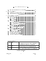
Document History:
ver 1.0 16. March 1995 Combined Programmer's Guide and User's Guide
into a single document and added description
of annular array design and 2D response
ver 2.0 15. August 1996 Moved advanced functions to separate document
General update, added tutorial introduction
ver 2.1 7. April 1998
Updated installation instructions
Added volumetric simulation and visualization
c 1996-1998
Copyright April 8, 1998
5
ver 2.1
ULTRASIM USER'S MANUAL April 8, 1998
6
ver 2.1
ULTRASIM USER'S MANUAL 1 INTRODUCTION
1.1 About Ultrasim
UltraSim is a Matlab toolbox for ultrasound wave simulation developed by
Vingmed Sound (VMS), Horten, Norway, Department of Physiology and
Biomedical Engineering (IFBT) and Department of Mathematical Sciences
(IMF), Norwegian University of Science and Technology, Trondheim, and
Department of Informatics (IFI), University of Oslo. UltraSim serves as
a standard platform for simulation programs concerning ultrasonic imaging
systems. UltraSim provides a tool for transducer and dome design, and will
increase the user's understanding of acoustic wave propagation in homogeneous and layered media.
UltraSim features :
• Annular, Phased, Linear or Curved array transducers in 1, 1.5, and 2
dimensions
• Free choice of transducer parameters :
aperture
Radius of curvature
# elements
• Free choice of frequency
• Pulsed or Continuous wave excitation
• Facilities for :
Electronic focusing
Quantization of electronic time delays
Apodization
• Homogeneous or layered media with smooth surfaces
• Acoustic Wave Field Simulations :
at a point
along a line
in a plane
• Annular array design tool
UltraSim also oers possibilities of simulations including losses in media and
reection losses at surfaces between media of dierent wave velocities.
April 8, 1998
7
ver 2.1
ULTRASIM USER'S MANUAL 1.2 About Matlab
Matlab is a computer programming language supplied by the Mathworks Inc.
which is particularly advantageous for use with numerical calculations and
also provides powerful routines for handling graphics. The language is object
oriented, and is mainly based on C and Fortran. Some knowledge of Matlab
will be advantageous when using UltraSim, but it is not required.
1.3 About this document
The present document is written as an introductory document and reference
book to UltraSim. UltraSim's menu system should be self-explanatory to
a large extent and reading the entire document should not be necessary.
However, if this is your rst acquaintance with UltraSim, you are adviced to
read the rest of the Introduction section and then load the examples described
in the tutorial. Then read the section on Simulation of Acoustic Fields and
use the subsequent sections as a guideline when making the conguration for
your rst simulation.
Instructions for installation and for programming UltraSim may be found
in the Appendices.
A link to the latest electronic version of this document may be found on
http://www.i.uio.no/~sverre .
1.4 History
The program started as a Matlab toolbox called ARRAY. It was developed at
Vingmed Sound for simulation of array systems in 1990-91 and was designed
by Sverre Holm and Trond Kleveland who both have been following the
project since then.
Other contributors have been:
• Tor Arne Reinen (SINTEF-DELAB, 1992) - Start of 2D array module.
• Lars Ødegaard (Dr. Ing. student IFBT/IMF, 1992-1996) - Wave propagation in layered media[13].
• Vebjørn Berre, IFBT scientist 1992-1993) - Renamed program to ULTRASIM, made it compatible with MATLAB 4.0, and designed menu
system and new data structures.
• Kari Lervik (Siv. Ing. IFBT, 1992) - Start of 1.5D module.
• Espen Iveland (Siv. Ing. IFBT, 1993) - Annular array optimization.
April 8, 1998
8
ver 2.1
ULTRASIM USER'S MANUAL •
Frode Teigen, IFBT (scientist 1993-1994) - Completed 1.5D, upgraded
beam pattern module to energy summation and input of measured
pulse, worked with Lars Ødegaard on layered module, plus did general
upgrading.
•
Jan Ove Erstad (Cand. Scient. IFI, 1993-1994) - Coarray module and
Remez optimization module for thinned arrays [10].
•
Bjørnar Elgetun (Cand. Scient. IFI, 1994-1996) - Completed movie
module, improved user interface, made optimization programs for thinned
2D arrays [12].
•
Einar Halvorsen, IFBT (scientist 1995-1996) - Worked with Lars Ødegaard on layered module.
•
Kapila Epasinghe (Cand. Scient. IFI, 1995-) - Made volume and slice
simulations and C, and parallel computer versions of 2D response computation [14].
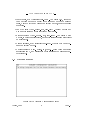
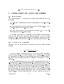
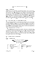
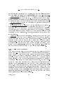
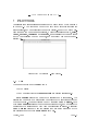
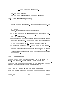
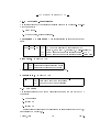
1.5 Getting started
Figure 1: The UltraSim Conguration window
April 8, 1998
9
ver 2.1
ULTRASIM USER'S MANUAL To start UltraSim from a UNIX system you rst have to start Matlab with
the command matlab in an xterm window. Then UltraSim may be started
with the command usim, which makes two graphic windows with a menu
bar each pop up. The xterm window where you start UltraSim will later
be referred to as the text window. The Plottool window, where the results
are plotted, will be described in section 7. Figure 1 shows the Conguration
window, where the conguration needed to perform a simulation and the
method of simulation are selected. The important items on the menubar
on top of the UltraSim Conguration window will be described in detail in
sections 4 - 6. However, it will be adequate to give some introductory remarks
here.
If this is the rst time Ultrasim is started for this user, a system startup
le will be read (from directory given in ULTRASIMHOME variable). Each
time one exits Ultrasim using the File, Quit Ultrasim or File, Quit Matlab commands, the present setup is saved in the user's startup.cnf le (in
directory given in USER_ULTRASIMHOME variable). This le is then
automatically loaded when Ultrasim is again started.
To set up a conguration and perform a simulation, start with the menu
items to the left on the menu bar, and progress towards the right.If you
already have saved a conguration for a simulation, choose the option Load
Conguration in the File menu. Files are saved with name *.cnf (old
format had le name *cnf.mat). There are example setups available under
the read-only directories for various kinds of transducers and simulations.
If you want to change the setup, you have to go through all the submenus
of SetFlags to set the basic properties of the conguration, as described
in subsection 4.1. Then you should set the conguration parameters in the
Conguration submenus, as described in subsections 4.2 - 4.3. If you are
particularly satised with the set-up and want to save it for later use, you
may do so by selecting Save Conguration in the File menu.
When the conguration is set, you are ready to start a simulation from the
Calculations menu, as described in section 6. You also have the possibility
of verifying your conguration graphically, by selecting one of the options in
the View menu. This is looked into in section 5.
The remaining options refer to the graphic display of the Conguration
window. Print produces a hardcopy or a Postcript le of the graphic contents
of the window. Note that selecting an item in the View menu will produce a
graphical output in the Conguration window (cf. section 5), while running a
simulation produces a graphical output in the Plottool window (cf. sections
6 & 7). Clear clears the graphic display, while Subplot allows you to
split the screen into several parts (subplots) before plotting. Colormap and
Shading applies to the cases where a 3D surface is plotted in the window.
April 8, 1998
10
ver 2.1
ULTRASIM USER'S MANUAL Colormap lets you change the color of the surface, while shading lets you
choose between three dierent shading styles on the surface.
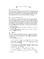
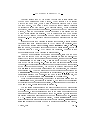
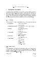
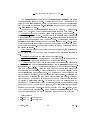
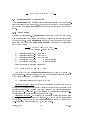
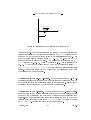
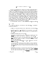
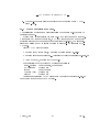
1.6 How to set the coordinates
z
ϕ
r
Transducer
x
θ
y
Figure 2: Coordinate system of UltraSim
In UltraSim you have a choice between using Carthesian and spherical
coordinates. Figure 2 demonstrates how both the Carthesian (x,y,z) and
the spherical (r,θ,φ) coordinates at the point marked with an asterisk are
dened. As can be seen from the gure, the origin of UltraSim's coordinate
system is placed at the center of the transducer, so that the beam center
of the emitted ultrasound wave coincides with the z-axis. There are two
exceptions to the last statement. First, the beam from a linear array may be
steared o the z-axis. This will not change the position of the transducer.
Secondly, the annular transducer may be tilted relative to the z-axis if you
are planning on using simulation option Layers and comments to Rotation
angle in subsection 4.3.1).
Note that when using the simulation option Layers, only two dimensions
are used, and that the coordinate system coincides with the xz-plane of g.
2. Note also that the z-axis is the abscissa and the x-axis the ordinate of this
2D coordinate system.
A standard rectangular transducer has its elements distributed along the
x-axis. Standard azimuth beamproles are obtained by setting θ = 0 and
vary φ at a xed value of r.
April 8, 1998
11
ver 2.1
ULTRASIM USER'S MANUAL April 8, 1998
12
ver 2.1
ULTRASIM USER'S MANUAL 2 TUTORIAL
Go through these examples rst to familiarize yurself with the basic features
of Ultrasim. Each example is loaded by entering File, Load, 2) Ultrasim
examples. The transducer geometry can be viewed by View, Transducer,
2D-plots and the parameters can be inspected by going through all the
submenus in the Conguration menu.
2.1 Example 1 - Beam pattern in focus
Load 'e1-bpfoc.cnf' and compute by Calculations, Beam-Pattern, Peak
Calculation or Calculations, Beam-Pattern, Energy Calculation to
get the beam pattern for an annular array from -50 to 50 degrees in focus
(range 78 mm).
2.2 Example 2 - On-axis eld
Load 'e2-bpax.cnf' and compute by Calculations, Beam-Pattern, Peak
Calculation to get the beam pattern for an annular array on the axis for
range 1 to 100 mm.
2.3 Example 3 - 2D response, pulsed grating lobes
Load 'e3-2dgr.cnf' and compute by Calculation, 2D response, Compute response. Visualize the result by the command Calculation, 2D
response, Surface plot using default values for the parameters. The result
is pulsed grating lobes for a linear array with a pitch of 2 lambda. The result may also be visualized using the Contour plot or the Color-encoded
commands in the same menu.
2.4 Example 4 - 2D response, continuous wave
Load 'e4-2dcw.cnf' and compute by Calculation, 2D response, Compute response. Visualize the result by the command Calculation, 2D
response, Surface plot using default values for the parameters. This is
the continuous wave eld from a phased array with pitch = lambda/2. The
eld may also be visualized using the Calculation, 2D response, Contour
plot command. Instead of using default values, you should reect the plot
about the z-axis. If the 'iso' option is used, one gets a contour plot of the
beamwidth showing clearly the eect of focusing.
April 8, 1998
13
ver 2.1
ULTRASIM USER'S MANUAL 2.5 Example 5 - 2D response, moving pulse
Load 'e5-2dmov.cnf' and compute by Calculation, 2D response, Compute response. Visualize the result by the command Calculation, 2D
response, Surface movie using default values for the parameters. The result is 11 simulations of a pulse travelling in depth containing pulsed grating
lobes.
2.6 Benchmark calculation
The le 'benchmrk.cnf' contains a simulation intended for measuring the
relative performance of the computer. It is small enough to run on a Pentium PC with 8 Mbytes of RAM without paging, thus only CPU power is
measured. Typical performance is:
•
•
•
•
•
SUN Sparc 2: 71 sec
DEC 5000/240: 37.5 sec
Pentium 90 MHz (Windows 95): 32.5 sec
IBM RS6000: 11 sec
DEC alpha: 9.8 sec
These execution times are computed using the m-le version of the Calculation, 2D response, Compute response command. There is also a
C-version (Mex-le) that will improve performance by a factor of 3-4.
The result can be visualized using the Calculation, 2D response, Surface plot using default values for parameters.
April 8, 1998
14
ver 2.1
ULTRASIM USER'S MANUAL 3 SIMULATION OF ACOUSTIC FIELDS
3.1 Introduction
In medical ultrasound a whole range of various transducers are common,
including:
1. Pre-focused annular arrays divided into rings using the equal-area principle
2. Rectangular arrays divided into elements of dimension 0.5 - 2 λ with
pre-focusing in the short-axis dimension
3. Curved arrays divided into elements of dimension 1 - 2 λ with prefocusing in the short-axis dimension
In addition there is need to understand the properties of transducers of
more complex shapes such as oval or elliptic ones, and to nd the elds
generated by 2-dimensional transducers. For this reason Ultrasim, a general
purpose simulator tool has been made. This chapter is adapted from [11].
3.2 Method and Examples
In order to nd the eld it is common to assume that the Rayleigh integral
applies:
1
φ=
2π
Z Z
un (r0, t − r/c)
dS
r
where the velocity potential is given by the normal velocity integrated
over the active surface. The source is assumed to be plane, i.e. the lateral
dimensions and the radius of curvature are large compared to the wavelength
[2], and thus curved transducers used in ultrasound are covered by this assumption.
In the impulse response method the Rayleigh integral is converted from a
2-dimensional to a 1-dimensional integral [1]. This assumes that the diraction impulse response has been derived for the transducer shape used. In the
described simulator, this method is not used. One of the reasons is that it
is desirable to be quickly able to analyze new transducer shapes. This could
also be done using the impulse response method by subdividing the radiating plane into smaller basic subtransducers with a known diraction impulse
response [4]. However it is also desirable to be able to analyze the eld in an
April 8, 1998
15
ver 2.1
ULTRASIM USER'S MANUAL inhomogenous medium. One of the underlying assumptions of the impulse
response method is that the path from the radiator to the summation point
is independent on actual position. Thus this method has limitations when
the eld is to be found in an aberrating medium. In this case one has to
give up the speed advantage and solve the Rayleigh integral directly taking the medium properties into account for each path from source to eld
point [8],[9].
The Rayleigh integral is solved by discretizing the radiating surface, assuming that the plane source vibrates in a single mode (thickness mode) [3],
and thus that the surface velocity is separable:
un (r, t) = O(r) · u(t)
The observation plane is also discretized and the integration is done by
nding the distance and quantized time delay [7] from each source point to
each of the observation points. The time waveform is either continuous wave
or a pulse that resembles the pressure pulse measured at the focal point on the
acoustical axis. At this point one will get coherent summation of the Rayleigh
integral. This means that we excite with a measured approximation of the
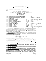
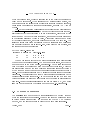
surface velocity. The following four gures give examples of the output from
the simulator. In addition it is possible to generate animations of travelling
ultrasound pulses using the display of Fig. 4, or to take the maximum at all
locations of an animation and generate a contour plot like in Fig. 3
April 8, 1998
16
ver 2.1
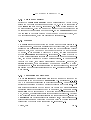
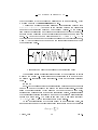
ULTRASIM USER'S MANUAL ARRAY−RESPONSE Reference=38.96 [us]
6−FEB−1995 15:51
Theta=0 [deg] Phi=0 [deg] N=64 M=1 f=3.5 [MHz] pitch=0.5 osc=Inf
Azimuth : no apodization
Elevation : no apodization
BEAMWIDTH [dB], Aperture (AZ) 14.08 [mm]
10
8
6
−6
4
−12
2
0
−2
−6
−12
−4
−6
−8
−10
10
20
30
40
50
60
70
80
Range in [mm], Azimuth focus=60 [mm] Envelope
90
100
Figure 3: Plot of beamwidth contours (-6, -12 and -20 dB) for a 64 element
array with half lambda pitch at 3.5 MHz, focus = 60 mm.
ARRAY−RESPONSE Reference=38.96 [us]
6−FEB−1995 15:58
Theta=0 [deg] Phi=0 [deg] N=64 M=1 f=3.5 [MHz] pitch=0.5 osc=3
RESPONSE [lin]
Weighted−envelope
Azimuth : no apodization
Elevation : no apodization View: 3D default
60
40
20
0
10
100
5
80
0
60
40
−5
Aperture (AZ) d=14.08 [mm]
−10
20
0
Range in [mm], Azimuth focus=60 [mm]
Figure 4: Plot of pulse in focus as sent from the same array as in Fig. 3.
Pulse form is 3 periods shaped with a cosine.
April 8, 1998
17
ver 2.1
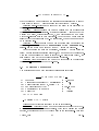
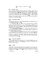
ULTRASIM USER'S MANUAL Beampattern (delays set for steering to fixed point, source moves)
[dB], focus at 60.00 mm, steered angles = (0, 0) degrees
0
6−FEB−1995 16:06
−5
Frequency = 3.5 MHz
−10
−15
−20
−25
−30
−35
−40
−60
−40
−20
0
20
40
60
3 periods, cosine pulse, no delay quantization, azimuth [deg], el = 0, observed at 60.00 mm
Figure 5: Beampattern obtained by summing energy over all time at a distance equal to geometric focus (60 mm).
Beampattern (delays set for steering to fixed point, source moves)
[dB], focus at 60.00 mm, steered angles = (0, 0) degrees
10
8
6−FEB−1995 16:01
6
Frequency = 3.5 MHz
4
2
0
−2
−4
−6
−8
0
10
20
30
40
50
60
70
80
90
100
Inf periods, rectangular pulse, no delay quantization, radius [mm], el = 0, az = 0
Figure 6: Intensity plot along acoustic axis for continuous excitation for array
of Fig. 3.
April 8, 1998
18
ver 2.1
ULTRASIM USER'S MANUAL 4 CONFIGURATION
This section gives a description of how to set up a conguration previous to
performing a simulation. If you are using UltraSim for the rst time you
are adviced to study this section thoroughly, as knowledge of the UltraSim
Conguration is a requirement for a correct interpretation of the simulation
results. You may however skip the sections marked 'Advanced', unless you
are planning to use the option(s) described in an 'Advanced' section.
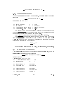
4.1 SetFlags
There are six submenus to the SetFlags menu, with the following options :
Focus Mode
Fixed Focus (Default)
Dynamic focus
TransducerGeometry Rectangular and Curved Array (Default)
Annular Array
Medium
Homogeneous (Default)
Layered 2D
Layered 3D
Coordinates
Rectangular (Default)
Spherical
k-space (sin(angle))
pitch/mm
[mm] (Default)
pitch (ref. to lambda)
Observation
Point
Line (Default)
Plane
Plane -> Movie
Volume
Volume -> Movie
4.1.1 Focus Mode
The Focus Mode ag should start in its default value, Fixed Focus. Setting
the ag to Fixed Focus, allows you to set an electronic focus to a point, as
described in section 4.5. The impact of setting the ag to Dynamic Focus is
described in subsections 4.5.3, and 6.2.
April 8, 1998
19
ver 2.1
ULTRASIM USER'S MANUAL 4.1.2 Transducer Geometry
Setting the TransducerGeometry ag to Rectangular and Curved Array,
allows you to choose a rectangular or curved 1D, 1.5D or 2D transducer in
the Transducer submenu (cf. subsection 4.3). You may also choose to use
an oval transducer. With the ag set to Annular Array the transducer will
be annular with an arbitrary number of rings. In the Transducer submenu
you are allowed to choose between Equal Area and Equal Width rings, and
two additional options, which are described in subsection 4.3.
4.1.3 Medium
The Medium ag denes whether the medium used in the simulation is ho-
mogeneous or not. You should generally use the default value, Homogeneous,
unless you are particularly interested in examing wave propagation through
layered media, when you would want to use the Layered 2D or the Layered
3D option. If you are using a Layered 3D medium, you also must use one
of the Beampattern simulations (cf. subsection 6.1). Using a Layered 3D
medium will substantially increase the amount of time needed for a simulation, and should therefore be avoided unless necessary. If you are using a
Layered 2D medium, time consumption will not be a problem. However, the
Layers simulation, which is obligatory when using a Layered 2D medium,
is restricted to on-axis simulations using an annular transducer, since this
simulation method exploits rotational symmetry. See also subsection 4.6 for
more details.
4.1.4 Coordinates and pitch/mm
The Coordinates and pitch/mm ags lets you choose the format of the
parameters in the submenus of Conguration (cf. subsections 4.4 - 4.3).
You may use either rectangular or spherical coordinates. For spherical coordinates the angles may either be specied directly or by their sines. The
last option is for display in the wavenumber domain and gives possibilities
for setting sines that are larger than 1 in magnitude, i.e. imaginary angles.
pitch/mm may be set to either mm (implying that all distances are given in
mm), or pitch, when all distances are given in units of wavelengths. Note that
when observing along a line transversal to the transducer normal, setting the
Coordinates ag to rectangular gives a straight line, while choosing spherical coordinates gives a curved line where each point on the line are equally
distant from the center of the transducer (cf. subsection 4.7).
April 8, 1998
20
ver 2.1
ULTRASIM USER'S MANUAL 4.1.5 Observation
The selection of the observation ag is strongly related with the type of simulation you want to use. Observation at a point is only compatible with the
(2D) layered medium simulation. If you are planning to use this simulation
method, you may also choose to observe along a line, which is also the only
possible option when performing a beampattern simulation (cf. subsection
6.1). Observation in a plane or volume and time-varying observations in a
plane or volume (movie) is only possible when conducting a 2D response
simulation (cf. subsection 6.2). See also subsection 4.7 for more details.
4.2 Conguration Submenus - General
The remaining subsections of this section concentrate on the submenus of
the Conguration menu. With the exception of List, all the Conguration
submenus control one part each of the conguration necessary for running a
simulation. All the submenus are displayed in the Matlab text window, and
they all display the parameters on the same format with the exception of the
Medium submenu for the layered medium:
No.) Parameter Name : Value
The Transducer submenu, which is given below, is a typical example.
To change the value of one parameter, type the No. which is preceding the
parameter name at the input prompt. When you have made the changes
you want to do, simply press <CR> ('Enter') to exit the submenu. The No.
is the array index in the variable for this menu (except for the Observation
menu), see appendix for more details.
4.3 Transducer Parameters
4.3.1 Annular Array
- TRANSDUCER SUBMENU - ANNULAR ARRAY Input is in [mm] units
lambda = 0.22 mm
18)
9)
1)
2)
3)
Transducer type
Fixed focus
Transducer aperture
# elements
# points
April 8, 1998
F
D
N
P
:
=
=
=
=
21
Equal Area
50.00 mm = 113.64 lambda
12.00 mm = 27.27 lambda
4
1500
ver 2.1
ULTRASIM USER'S MANUAL The Transducer submenu when the TransducerGeometry ag is set
to annular array is shown above. The line Input is in [mm] units shows the
value of the pitch/mm ag, while the wavelength (lambda) is calculated
from the values of Frequency (cf. Excitation submenu) and Speed of Sound
(cf. Medium submenu).
Note that when the Medium ag is set to 2D Layered, # points is replaced by # rays, and two additional options are included (See below).
Transducer Type can be either Equal Area (default), Equal Width, Circular or User-Dened Width. Equal Area is an annular array transducer
where all rings have the same surface area. Equal Width is an annular array
transducer where all rings have the same width. Circular is a transducer
consisting point sources spread around the perimeter of a ring. User-Dened
Width is an annular array transducer on which the user may choose the width
of each ring as he likes. The user will be asked to make a choice only after a
simulation is started.
Fixed Focus is the Radius of Curvature of the transducer, and corresponds
to the depth at which the beam will be focused if no electronic focusing is
set.
Transducer aperture is the diameter of the transducer.
# elements is the number of rings on the transducer, or the number of
point sources if Transducer type is set to Circular (see above).
# points refers to the number of points used to represent the transducer
when simulation methods Beampattern and 2D Response are used (cf.
subsections 6.1 & 6.2). The points are distributed over the transducer's surface on a hexagonal grid. Using sucent number of points is important for
the reliabilty of the results, while choosing too many points will lead to an
unnecessarily long computation time. The optimal number of points to use
depends on the frequency, and the observation conguration. Increasing the
frequency and observing far from focus will require more points, while low
frequencies and observation in focus reduce the number of points required
to perform a reliable simulation. As a rule of thumb the points should be
separated by approximately half a wavelength, unless when observing close
to focus when the # points may be reduced, and when observing at extreme
regions (in the extreme near-eld or very far from the beam-center), when
the # points should be increased. When quitting the Transducer submenu,
the point separation in mm and wavelength is given as in this example:
point distance
x : 0.2459 mm, 0.479 lambda
y : 0.2129 mm, 0.4148 lambda
April 8, 1998
22
ver 2.1
ULTRASIM USER'S MANUAL 4.3.2 Rectangular and Curved Array
TRANSDUCER SUBMENU RECTANGULAR AND CURVED ARRAY Input is in [mm] units
lambda = 0.44 mm
18) Transducer type (0-rectangular, 2-elliptic)
= 0
17) Radius of curvature (0-planar, <0-curved)
= 0.00 mm = 0 lambda
AZIMUTH:
1) Azimuth array-aperture
d
= 12.00 mm = 27.27 lambda
2) Azimuth # elements
Ne_az = 4
3) Azimuth # points per element
Np_az = 1500
ELEVATION (1-D):
5) Elevation array-aperture
a
= 1.00 mm = 2.27 lambda
6) Elevation # elements
Me_el = 1
7) Elevation # points
Mp_el = 10
9) Elevation Fixed focus
ri (F) = 50.00 mm = 113.64 lambda
Above is the Transducer submenu when the TransducerGeometry
ag is set to Rectangular and Curved Array. Note that when Elevation #
elements is set to 3 or 5, the transducer will be a 1.5D transducer, which is
described in the below subsection.
Transducer type is by default rectangular (p = 0). Entering a ? at the
prompt gives the options. The footprint can be set by changing the parameter
p in the equation for the footprint:
(
x p
y p
) +(
) =1
d/2
a/2
for p > 0
For negative values of p, an octagonal shape can be chosen (p = −8).
Radius of curvature is used to dene a radius of curvature for a curved
array by setting a negative value, ie. for obtaining a convex array. A positive
value gives a prefocused (concave) transducer in the azimuth direction; i.e.
sets the focal point in the xz-plane.
Azimuth array-aperture is the length of the array in the azimuth (x) direction.
Azimuth # elements allows you to set the number of transducer elements
in the azimuth direction.
Azimuth # points per element refers to the number of points used to represent the transducer when simulation methods Beampattern and 2D Response are used (cf. subsections 6.1 & 6.2). See the description of this item
in the transducer submenu for annular arrays (the above subsection). Note
April 8, 1998
23
ver 2.1
ULTRASIM USER'S MANUAL that the total number of points on the transducer is calculated as (Azimuth
# elements)*(Azimuth # points per element)*(Elevation # points).
Elevation array-aperture is the length of the array in the elevation (y)
direction.
Elevation # elements allows you to set a desired number of transducer
elements in the elevation direction. By setting Elevation # elements to 1 you
will get a 1D array, while setting it to 2, 4, 6 or higher gives you a 2D array
with equal-size elements in both directions. Note that 3 and 5 elements are
reserved for the special case of a 1.5D transducer, where the elements may
be of dierent size.
Elevation # points denotes the number of points used to describe the
transducer, when performing the Beampattern and 2D Response simulations. See the above comments to Azimuth # points per element.
Note that unlike the azimuth equivalent, Elevation # points holds the
total # points for all the elevation elements, and not on each of the elements.
This has been necessary in order to include 1.5D arrays (see below), the
elements of which may have dierent elevation apertures.
Elevation Fixed focus allows you to set the focal point in the elevation
direction; i.e. the focal point in the yz-plane.
4.4 Excitation Parameters
The excitation submenu with its default values looks like this:
EXCITATION SUBMENU 1) Frequency
: 7.00 MHz
9) Transmitted pulse length (# oscillations) :
0.0
10) Pulse Weighting (none = 0, cosine = 1) :
0
11) Sampling frequency (Fs)
: 100.00 MHz
12) Quantizing of Time Delays
:
O
13) Pulse Type
: Ultrasim
CHANGE = "number"
-> Decision (<CR> = exit):
Frequency is the (center) frequency of the emitted signal.
Transmitted pulse length is the number of periods of a Pulsed Wave (PW).
By setting this parameter to '0' or to 'Inf', which is the Matlab symbol for
innite, a Continuous Wave (CW) will be used in the simulations. Note that
April 8, 1998
24
ver 2.1
ULTRASIM USER'S MANUAL some simulations will require a PW emission, namely the Layers simulation
and the Energy simulation in the Beampattern submenu (cf. section 6.1).
Pulse Weighting applies only to the PW case, and the emitted pulse will
have a cosine envelope if it is set to 1. The emitted pulse with a cosine
envelope corresponds reasonably to the pulses emitted from a real transducer.
No envelope is added to the PW signal when Pulse Weighting is set to zero.
Sampling Frequency is used for quantizing the electronic focusing time
delays. It is described below.
If Quantizing of Time Delays is On the the electronic time delays (cf.
subsection 4.5) are quantized with a quantizing time step of 1/fsample . If
Quantizing of Time Delays is O (Default) the electronic time delays are
not quantized, and thus the sampling frequency is not used. Therefore,
the sampling frequency is not displayed in the excitation submenu when
Quantizing of Time Delays is O. However, it is included in the above menu
for convenience.
Pulse Type should be set to its default, Ultrasim, except when you want
to use a pulse which may not be presicly dened by the above Frequency,
Transmitted pulse length and Pulse Weighting parameters. Normally this
exception occurs when you want to use a pulse which has been measured
experimentally. Also note that setting Pulse Type to any other value than
the default will work only if you plan to run an Energy simulation, which
is found in the Beampattern submenu (cf. subsection 6.1). Below the
somewhat tricky operation of using a User Dened pulse is described.
4.4.1 Pulse Type (Advanced)
The Pulse Type option allows you to choose between the pulse dened in the
above menu (i.e. The pulse is dened by the parameters set in options 1),
9) and 10)) and a User Dened pulse (usually an experimentally measured
pulse). Pulse Type Ultrasim designates a pulse as dened in the excitation
submenu, while a User Dened pulse must be dened by the user in a global
vector, pvector. A User Dened pulse overrides the values of the Frequency,
Transmitted pulse length and Pulse Weighing parameters, and as a consequence the Transmitted pulse length and Pulse Weighing parameters are not
displayed in the Excitation submenu if a User Dened pulse is to be used.
However, the Frequency still has to be set to a value approximately equal to
the frequency of the user dened pulse, as this frequency will be used when
calculating an appropriate sampling frequency (not to be confused with the
Sampling frequency in the Excitation submenu) for sampling the observed
signal (see subsection 6.1 for details). Note that the use of a User Dened
pulse will require some knowledge of Matlab.
April 8, 1998
25
ver 2.1
ULTRASIM USER'S MANUAL pvector must be dened before selecting the Excitation submenu, and is
to be on the following format:
•
Dene the vector as global; Write global pvector.
•
Element #1 of the vector (i.e. pvector(1)) is the time steps between
each of the following elements. Thus pvector(1) · (#elements − 2) will
be the duration of the pulse described by pvector.
•
The remaining elements of pvector are the amplitudes at time
−pvector(1) · (elementno. − 2). Thus pvector(2) is the amplitude at t
= 0, pvector(3) is the amplitude at t = - pvector(1) and so on. The
negative sign accounts for the fact that the start of the pulse is dened
to be at t = 0.
•
The length of pvector (# elements) may be chosen arbitrarily. Increasing # elements will increase the resolution, but increasing # elements
beyond 1000 will have no eect as UltraSim will convert pvector to a
vector holding 1000 elements in any case.
•
The pulse amplitudes may also be chosen arbitrarily, since the amplitudes will be normalized at a later stage, i.e. only the amplitude
relative to the maximum amplitude is considered.
When pvector is dened, choose the Excitation submenu, and select option
13), Pulse Type. Then choose User Dened from the menu which is displayed. When quitting the Excitation submenu, pvector will be converted
to a standard UltraSim format, and stored in the variable pvec, which will
be used as excitation signal when running an Energy simulation (cf. subsection 6.1. Note that if User Dened is chosen as pulse type and pvector
is not dened, a warning will be displayed, and Pulse Type will be set to its
default, Ultrasim.
There is also a third Pulse Type option: User Dened - Individual pulses
for each element, which allows you to dene the emitted pulse from each
of the elements of a transducer. To use this option N vectors, pvector1,
pvector2,..., pvectorN (N is # elements on the transducer), have to be dened.
The vectors must be on the same format as pvector above, and the pulse
emitted from transducer element no. n (1 ≤ n ≤ N) must be dened by
pvectorn. This option will normally be useful with transducers with a small
number of elements such as annular transducers, where the inner ring is
element no.1 , and the outer ring has the maximum element no. (N ).
April 8, 1998
26
ver 2.1
ULTRASIM USER'S MANUAL 4.5 Beamforming Parameters
The Beamforming submenus control the electronic focusing and the apodization (weighting) of the transducer. There are two dierent menus depending
on the value of the Focus Mode ag; one for xed focus and one for dynamic
focus.
4.5.1 Fixed Focus
As stated in subsection 4.1, Focus Mode ag should be set to Fixed Focus,
with the exception of the case which is commented on in the next subsection
(Dynamic Focus). The Beamforming submenu for the case of xed focus
looks like this when the TransducerGeometry ag is set to Rectangular
and Curved Array:
BEAMFORMING SUBMENU Fixed focusing - transmit mode
2) Electronic focusing - x [mm] : 0
3) Electronic focusing - y [mm] : 0
4) Electronic focusing - z [mm] : 100
5) Apodization Azimuth
: no apodization
6) Apodization Elevation
: no apodization
Parameters used in focusing algorithm:
14) Speed of Sound c [m/s] = 1540
Note that when the TransducerGeometry ag is set to Annular Array, focusing o-axis is impossible, and the three options Electronic focusing
x/y/z will be replaced by the single option:
4) Electronic focusing depth [mm] : 100
Electronic focusing depth gives you the possibility of speciying a depth
to which the transducer will focus by setting time delays on the rings of an
annular transducer. By setting this depth equal to the transducer's radius
of curvature (cf. subsection 4.3) you will turn o the electronic focusing; i.e.
the electronic time delays are zero on each element.
Electroning focusing - x/y/z allows you to specify a point rather than just
a depth, to which the transducer will focus. x, y and z are the coordinates
of the point. Note that when the Coordinates ag is set to Spherical the
xyz-coordinates will be replaced by r, phi and theta.
April 8, 1998
27
ver 2.1
ULTRASIM USER'S MANUAL Apodization Azimuth/Elevation lets you choose between the following
apodization (weighting) functions, in the azimuth and elevation directions:
0.
1.
2.
3.
4.
No Apodization
Hamming
Hanning
Kaiser-Bessel
User-Dened
To get an idea of the nature of the above apodizing functions, select an
apodizing function in the Beamforming submenu, and look at the resulting
weighting by choosing Apodization in the View menu (cf. subsection 5.6).
Note that when the TransducerGeometry ag is set to Annular Array,
the 2 options Apodization azimuth/elevation are replaced by a single option
for choosing apodization. Also the Kaiser-Bessel Apodization will not work
for annular transducers.
Speed of Sound refers to the value used in the focusing algorithm, which
calculates the electronic time delays for focusing to a point [8]. This value for
the speed of sound should not be confused with the value set in the Medium
submenu, which is the actual sound velocity in the medium (cf. subsection
4.6). Normally Speed of Sound should not be changed from its default value,
1540 m/s, which is an approximate average speed of sound in human tissue.
4.5.2 Additional focusing algorithm parameters (Advanced)
You will get the following two options if your Medium and TransducerGeometry ags are set to Layered 2D and Annular Array respectively:
15) Transducer diameter D : Real Transducer Diameter is used
16) Radius of Curvature ROC : Real Transducer ROC is used
Like Speed of Sound, which is commented on in the above subsection,
these parameters refer to the values used in the focusing algorithm [8], and
they should normally equal the actual transducer diameter and radius of
curvature, which are set in the Transducer Submenu (cf. subsection 4.3).
4.5.3 Dynamic Focus (Advanced)
The current version of UltraSim supports dynamic focus, only when the
Medium and TransducerGeometry ags are set to Layered 2D and Annular Array respectively or when the em 2D response calculation is used with
April 8, 1998
28
ver 2.1
ULTRASIM USER'S MANUAL rectangular arrays. When the Focus-mode ag is set to Dynamic Focus,
you will get the following Beamforming submenu:
BEAMFORMING SUBMENU Dynamic focusing - 2-way mode
Receive:
19) Number of focal zones
: 0
20) Start depth of rst focal zone [mm] : 0
21) End depth of last focal zone [mm] : 0
Transmit:
2) Number of focal zones
: 0
3) Start depth of rst focal zone [mm] : 0
4) End depth of last focal zone [mm] : 100
5) Apodization
: no apodization
Parameters used in focusing algorithm:
14) Speed of Sound
c [m/s] = 1540
15) Transducer diameter
D
: Real Transducer Diameter is used
16) Radius of Curvature
ROC : Real Transducer ROC is used
17) Focus mode
: 2-way
18) Calculation of Electronic Delays
: Focusing Algorithm
The rst line in the submenu, Dynamic focusing - 2-way mode, tells you
the value of the Focus-mode ag and the choice made on option 17), Focus
mode.
The Focus mode options lets you choose to focus on Transmit, Receive or
both (2-way).
Dynamic focusing is not usually used on transmit due to loss of frame
rate, but it may be interesting to simulate the eect of two or three zones
on transmit. If you do two-ways simulations, both the transmitted and the
received beam prole are plotted. The sum of the dB-versions of the two
beams are presented in the same plot.
There are three ways to specify the dynamic focusing of annular array
transducers. In the rst one, you may set the number of electronic focal
zones you want to spend. You may also specify the minimum and maximum
observation depth. Ultrasim will spread the foci between these two depths.
This is done in a way that minimizes the phase aberrations. In the second
alternative, you may add extra delays to the delays set by the automatic
algorithm. You can add one delay for each element. These extra delays
are constant for all observation depths. It is thus possible to correct for
phase aberrations caused by the dome. The third alternative is a manual
April 8, 1998
29
ver 2.1
ULTRASIM USER'S MANUAL specications of the positions and the delays of each zone, which allow you
to set the delays as in a scanner.
The menu's options will be adjusted according to the choice of Focus
mode, as will become clear from the description below.
Following Receive:, there are three parameters that dene the receive
focusing. Obviously, these become redundant when Transmit is chosen as
Focus mode, and they also are omitted when Calculation of Electronic Delays
is set to Manual (see below). Likewise, the transmit parameters are not
included in the submenu when Receive is chosen as Focus mode or when
Calculation of Electronic Delays is set to Manual.
Number of focal zones gives the number of zones to which UltraSim sets
a focal point. Note that you will get 'ideal' focusing to every observation
point if you set this parameter close to innite.
Start depth of rst focal zone and End depth of last focal zone dene the
region over which the focal zones will be (equally) distributed. Note that if
you set the start depth equal to the end depth and Number of focal zones to
1, you get the xed focus case. This procedure will be useful (and necessary)
if you want to set a xed focus when transmitting, and use a dynamic receive
focus.
Apodization is explained in the previous subsection.
The remaining parameters refer to the focusing algorithm for calculating
electronic time delays. See the previous subsection for an explanation of
Speed of Sound, Transducer diameter and Radius of Curvature.
Calculation of Electronic Delays gives you the choice between the following options:
0) Focusing Algorithm
1) Focusing Algorithm with the addition of constant delays
2) User-Dened Electronic Delays
Choosing Focusing Algorithm tells UltraSim to use the focusing algorithm
when calculating the electronic time delays.
Focusing Algorithm with the addition of constant delays also uses the focusing algorithm. However you may add a constant time delay to each element in addition to the delays calculated by the focusing algorithm. When
choosing this option, a new option appears in the submenu:
22) Constant delays - el.1-5 [ns] - transmit: [ 0 0 0 0 0 ]
The above example is given for an annular array of 5 rings. The rst
element of the delay vector gives the delay on element #1 on the transducer,
April 8, 1998
30
ver 2.1
ULTRASIM USER'S MANUAL which is the inner ring, while the last element of the delay vector gives the
delay on the outer ring. When selecting the Constant delays option, you
must either enter the entire vector of delays (in this example it is 5 elements,
don't forget to enclose the values in brackets: [ ]), or press <CR> for no
change.
User-Dened Electronic Delays allows you to freely set the delays for each
of the elements. Note that this option makes the three parameters that usually describe the dynamic focusing (Number of focal zones, Start depth of rst
focal zone and End depth of last focal zone), as well as the parameters used
in the focusing algorithm (Speed of Sound, Transducer diameter and Radius
of Curvature) redundant, and these will be removed from the submenu. The
following option will become available when the electronic time delays are
set manually (If focus mode is set to 2-way, there will be 2 new options, one
for transmit and one for receive):
22) Time delays - transmit:
rstart[mm] rstop[mm] delay el.1-5 [ns]
12
21
0 0 0 0 0
21
45
0 0 0 0 0
The number of rows in the above matrix for electronic time delays equals
the number of focal zones desired. The number of focal zones, and thus the
number of rows in the above matrix, is optional. The two leftmost columns
hold the values of the start and stop depths of each focal zone, while the
remaining columns show the time delays on transducer elements 1 (column
3) to 5 (column 7); In this example the annular transducer is divided into 5
rings. Note that transducer element #1 refers to the inner ring of the annular
transducer. The electronic time delay matrix is entered analogously to the
constant delays vector (see above). You have to enter one row at a time as a
vector containing the start and stop values and the delays on all transducer
elements. To use the original entries of a row simply press <CR>, and enter
'0' when you have reached the desired number of rows, i.e. focal zones.
4.6 Medium Parameters
The Medium submenu denes the characteristics of the medium through
which the acoustic wave propagates. The submenu for a homogeneous medium
is fundamentally dierent from the submenu for the (2D & 3D) layered
medium, and it will be adequate to treat the two submenus separately.
April 8, 1998
31
ver 2.1
ULTRASIM USER'S MANUAL 4.6.1 Homogeneous Medium
When the Medium ag is set to Homogeneous, the Medium submenu looks
like this:
MEDIUM SUBMENU Model : HOMOGENEOUS
1)
2)
3)
4)
Speed of Sound
c = 1540
Impedance
Z = 0 MRayl
Attenuation - alpha alpha = 0.000 1/(m*MHz)
Attenuation - beta beta = 0.000
The Speed of Sound is the propagation velocity of the acoustic wave in
the homogeneous medium. The default value of 1540 m/s corresponds to an
approximate average speed of sound in human tissue.
The Impedance is not used in the current version of UltraSim.
The Attenuation parameters, alpha and beta, are only used by the functions Spectrum with depth in the View menu and the Annular Array
Analysis menu, and they are used to calculate the frequency dependent
attenuation according to the equation:
I(r)
β
= eαf r
Io
Note that alpha is given in dB/cm/MHz. See subsection 5.2 for details.
4.7 Observation Parameters
The Observation submenu with its default values is as following, when the
observation ag is set to Line (default):
- OBSERVATION SUBMENU Linetype : LINE
Coordinates : RECTANGULAR
1) # pixels along one axis :
90
2) Selected axis
:
y
3) Start value of y
4) End value of y
[mm] : 0
[mm] : 30
5) Fixed value of x
6) Fixed value of z
7) Fixed value of t
[mm] : 0
[mm] : 100
[us] : 0
April 8, 1998
32
ver 2.1
ULTRASIM USER'S MANUAL Linetype and Coordinates, which are unsettable in this menu, show the
values of the ags set in the SetFlags submenus. Obviously, the Observation submenu will change if these ags are altered. Changing the Coordinates ag to Spherical will not only have the eect of changing the
coordinates from xyz to r, theta & phi, but will also alter the shape of a line,
if this is the Observation option selected; see below. Note that rectangular
coordinates must be used if you have chosen the Observation option Plane.
# pixels along axis refers to the resolution of the line. Increasing # pixels
will increase the resolution, which also will increase computation time of the
simulation. Obviously this option becomes redundant when choosing a Point
as Observation option. Also this option is replaced by:
15) # obs.pts /[mm]
:1
when the observation option is a Plane. This is just another way to dene
the resolution.
Selected axis can be x, y or z, and it refers to the axis to which the line is
parallel; the remaining coordinates will have a xed value for every point on
the line. It can easily be seen that if you are using spherical coordinates, the
line will be an arc if the selected axis is theta or phi. When the observation
option is a plane UltraSim will ask you to select two axes, to which the chosen
plane will be parallel. You are also allowed to select t (time) as one axis, see
the below subsection for details (Note that t is not used when observing along
a line or at a point). Obviously, all the values will be xed if the observation
option is a point.
Start value and End value of y (or x,z) give the extremeties of the line.
Thus, the line will be represented by (# pixels along axis) points equally
separated between the Start value and the End value of the Selected axis,
while the other coordinates (x and z in this example) will be xed. The
plane will be represented in a similar manner, only that the resolution is
dened in an alternative way; see above.
Fixed value of xyzt (r,phi,theta if spherical coordinates are chosen) determines a xed value for the coordinates which are not a selected axis (see
above). Note that t (time) is only used when observing in a plane, and that
when point is the observation option, all the values are xed.
4.7.1 How to set time when observing in a plane
Observation in the xy-plane. To set the time when observing in the xyplane you rst will have to nd the (average) distance from the transducer to
the plane where you are observing, which normally is approximately equal to
April 8, 1998
33
ver 2.1
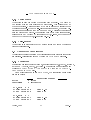
ULTRASIM USER'S MANUAL x
tpulse = 3/f
z
t propag=z/c
Figure 7: Calculation of propagation and pulse times
the xed z value. Then you can calculate the time at which the pulse from the
transducer arrives to the plane (propagation time: tpropag = distance/Speed
of Sound (t=z/c); Speed of sound is set in the Medium submenu). Note
that the pulse will be emitted at time = 0 - tpulse /2; i.e at time t = 0
half of the pulse is already emitted. The pulse time is calculated as tpulse
= # periods/f (cf. g. 7, where # periods is 3.). This is illustrated in
g. 7. Thus the time chosen should be in the approximate region t ∈
[(tpropag − tpulse /2), (tpropag + tpulse /2)] as there will be no signal outside this
region. Within these limits you may choose a time depending on which part
of the signal you want to observe.
Observation in the xz- or yz-plane. When observing in the xz- or yz-
plane it is convenient to choose the time so that all of the pulse or a maximum
of the pulse is within the observation plane at the actual time. See the above
paragraph for details on how the time should be calculated.
Observation in the xt-plane. When observing in the xt-plane it is nat-
ural to choose a time so that approximately all of the pulse passes the line
dened by the x values and the xed z and y values during the selected time
interval. For most practical tasks it suces to relate the time to the xed z
value so that Start value of t is set to z/c − tpulse /2 and End value of t is set
to z/c + tpulse/2. See also the above comments to gure 7.
April 8, 1998
34
ver 2.1
ULTRASIM USER'S MANUAL 4.8 Thinning and Weighting
The option for Array thinningcontains functions for thinning and perturbing an array as well as placing elements with spacing determined by a
geometric series. When asked to input numbers, this must be done in the
MATLAB command window. A local symmetry ag is indicated by ON/OFF
and is altered by pushing the 'x' button. When ON the thinning will remove
elements symmetrically around the array origin.
The option Optimize weights, will give the optimal apodization for the
current array. Optimality is dened in the Chebyshev sense, i.e. constant
sidelobe level. The apodization weights are put into the global matrix variable amp_ud (User dened apodization). User operation is performed by
pushing mouse buttons or a key on the keyboard, while pointing inside the
UltraSim conguration window. The rst function uses the formulation of
the Parks-McClellan Remez algorithm and thus can optimize equi-spaced arrays. For these arrays it will be the most ecient one to use. Input value is
the angle where the sidelobe level is desired to be reached (in degrees).
A second routine uses a generalized Remez algorithm formulation and can
be used to optimize weights for sparse, perturbed, and non-equally spaced
array as well as equi-spaced array [10]. The current version is user interruptable in every iteration. The 'x'-key should be pushed when asked to strike a
key. This has been useful with arrays that converge slowly, because a more
dense sampling then might help. (The sampling density is determined by
the 'Grid spacing variable' which has 16 as the default value. It has been
observed that in some cases a less dense sampling is more ecient.)
The input format is
[φ0p φ0s φ0O K]
Here φ0p is the cut angle for the mainlobe in degrees, φ0s is the angle
where one wants the equiripple sidelobe level to be reached, φ0O is the upper
limit for the optimization region and K is the approximation error weight
value (in most cases 10). The brackets must also be entered.
4.9 List
The last item in the Conguration menu, List, lists all the parameters set
in the submenus treated above. You may choose to list the parameters to
the screen or to a text-le.
April 8, 1998
35
ver 2.1
ULTRASIM USER'S MANUAL April 8, 1998
36
ver 2.1
ULTRASIM USER'S MANUAL 5 VIEW
The View menu is useful for verifying that your choice of parameters in
the Conguration menu is sensible. If you are new to UltraSim, you are
adviced to verify changes to the conguration, by selecting the appropriate
item in the View menu. Below, all the menu items are described briey, as
using these functions is the best way of getting acquainted with them.
5.1 Excitation - transmitted signal
This option plots the transmitted signal and its frequency spectrum. The
upper graph shows the time-domain signal, the amplitudes of which are normalized. The lower graph shows the frequency spectrum plotted for frequency
ranging from zero to 4 times the center frequency of the signal. Note that
there will be no graphical output when a CW-signal is transmitted.
5.2 Spectrum with depth
This option gives the transmitted spectrum and the spectrum at certain
depths in the medium using the Medium parameters for frequency dependent attenuation.
5.3 Observation
The Observation option displays the observation point, line or plane chosen
in the Conguration menu. Four plots are displayed; one 3D plot, and three
2D plots for the xy-, xz- and yz-planes respectively. Note that the proportions
of the plots may be somewhat misleading due to Matlab's autoscaling of the
axes.
5.4 Media
5.5 Transducer
There are two ways to view the Transducer : 2D-plots and Surface.
2D-plots plots the points used to represent the transducer in two dierent
projections. There is one plot for the xy-plane, and another for the xz-plane.
The second option, Surface, makes a plot of the transducer based on the
collection of points representing the transducer. The plot of the transducer
can be rotated and tilted and the shading and color can be changed. This
April 8, 1998
37
ver 2.1
ULTRASIM USER'S MANUAL works well for the transducers where the points are distributed on a rectangular sampling grid (rectangular and curved arrays). The transducers where
the points are distributed on a hexagonal grid (annular arrays) will not be
as smooth as desired in all cases.
5.6 Apodization
This option makes three plots describing the apodization. The rightmost
plot gives the apodization over the transducers surface, while the two plots
to the left gives the apodization along the azimuth and elevation directions.
If a 1-D transducer is specied only the upper left-hand gure will appear.
Note that a special case occurs when the equal area, annular transducer
is selected. UltraSim will automatically set an apodization on each ring to
compensate for the fact that there are an unequal number of points on the
rings, due to the fact that when UltraSim spreads the points on the transducer's surface more consideration are taken to get an equal spacing between
the points than to get exactly the same number of points on each ring. To
get an example of this phenomenon select the equal area annular transducer
and turn the apodization o, before selecting View Apodization. Note
that as the number of points used to represent the transducer increases, the
importance of this apodization decreases.
5.7 Delay
The Delay option has three submenus : Phase-centers, Exact delays and
Quantization Error.
Phase-centers plots the phase centers of the elements in three plots when
a rectangular transducer is used. The plots show the phase centers in the
xy-, xz- and yz-planes. There is only one plot for the annular array case, the
abscissa being the radial distance from the center of the transducer.
Exact delays shows the electronic time delays before they are quantized. If
the quantization of time delays is turned o, Exact delays will give the delays
that are used in the simulation. Three plots are given as for the apodization.
The plot to the right shows the delays on the transducers surface, while the
two plots to the left shows the delays on transducer elements in the x and y
directions. Note that the plots to the left are plotted for y = 0 and x = 0
respectively.
Quantization Error gives three plots; one plot of the exact time delays,
one plot of the time delays after they have been quantized, and one plot of the
relative quantizing errors. The relative quantizing error lies within [-0.5,0.5],
April 8, 1998
38
ver 2.1
ULTRASIM USER'S MANUAL and gives the quantizing error relative to the worst quantizing error possible
at the given sampling frequency.
Note that the values on the abscissa are pointers to where the transducer
points are stored in the internal UltraSim variable. This may be confusing
when the points are not stored elementwise. In fact the points are stored
elementwise for the 1D linear array only.
April 8, 1998
39
ver 2.1
ULTRASIM USER'S MANUAL April 8, 1998
40
ver 2.1
ULTRASIM USER'S MANUAL 6 SIMULATIONS
6.1 Beampattern
Beampattern simulates the ultrasound wave along a line in space, or to be
more correct the wave is simulated at points along a line. The method which
is used for the simulations is based on Huygen's principle of representing a
source by point sources and adding the contribution from all point sources in
order to get the resulting eld. The method for simulation in homogeneous
material is described below. This method is also the foundation for the
simulation method in a layered medium, which is looked into next.
6.1.1 Simulation Method - Homogeneous material
Figure 8: Illustration of the beampattern simulation method. The source is
the lower surface and the beampattern is found along the upper line.
As is demonstrated in the above gure, a pulse is sent from each transducer point at time ttransmit = to +∆ti −tpulse/2, where ∆ti is a time delay for
all points on element #i on the transducer. tpulse is the duration of the pulse.
Thus UltraSim sets the transmit time to be the time when half the pulse is
emitted. The delays will be calculated from the setting of an electronic focus
in the Beamforming submenu of the Conguration menu (cf. 4.5), and
by selecting View/Delays, you can see the values of the delays. Note also
April 8, 1998
41
ver 2.1
ULTRASIM USER'S MANUAL that the pulses may have dierent amplitudes due to an apodization, which
may also be set in the Beamforming submenu.
A pulse from a transducer point arrives at an observation point at time
tobservation = ttransmit + r/c; where r is the distance between the transducer
point and the observation point and c is the sound velocity. At the observation points the pulses from each transducer point are added as they arrive, in
order to get the pulse form at each observation point as shown in an example
in g. 9. Note that the time delays are all ∆ti = 0 and to = 0. rnear is
the distance to the point on the transducer closest to the observation point,
while rf ar is the distance to the point on the transducer farthest away from
the observation point.
1
0
-1
rfar /c + t pulse /2
r near /c - t pulse /2
Figure 9: Example of total pulse at the observation point
The resulting pulses at all observation points may be represented in either
a plot of the Energy vs. observation point coordinates or in a plot of Peak
amplitude vs. observation point coordinates. These methodes are described
below.
ENERGY
In g. 10 the pulses received at all observation points are merged in order
to get a 3D plot of the pulsed wave around the line of observation. Each line
along the radial direction (which also can be thought of as the time axis),
represent the pulse sampled at one of the observation points, while lines along
the transversal direction represent a sample of the pulses at all observation
points at a given time. The pulse is sampled with a sampling frequency
fs = 4 ∗ fo , where fo is the center frequency of the signal.
To get a representation of the pulse energy at an observation point, all
samples of the pulse at the observation point are squared and added together:
Energy =
X
s2n
n
April 8, 1998
42
ver 2.1
ULTRASIM USER'S MANUAL Rad
ial D
ista
nce
ce
a
vers
s
Tran
tan
l Dis
Figure 10: 3D plot of Beampattern pulse samples
where sn is pulse sample number n at the observation point. The energy is
normalized so that the energy in the focal point is 0 dB when no attenuation
is present. An example of the resulting beampattern energy curve, which is
displayed in the plottool window, is given in g. 11.
Beampattern - Energy
0
-5
energy [dB]
-10
-15
-20
-25
-30
-35
Transversal distance
Figure 11: Example of energy diagram
PEAK
The second option in the Beampattern submenu, Peak, uses the envelope of the wave when plotting the results. The envelope of the pulses
presented in the 3D-plot of g. 10 is shown in g. 12. Note that all the data
necessary to obtain the plot of g. 11 are not calculated when using the Peak
April 8, 1998
43
ver 2.1
ULTRASIM USER'S MANUAL 1
Amplitude
0.8
0.6
0.4
0.2
0
50
40
100
30
80
60
20
40
10
Radial Distance
20
0
0
Transversal Distance
Figure 12: Envelope of the pulses presented in g. 10
option. Instead, only the line along the transversal direction, which has the
highest amplitude is calculated as shown in g. 13. Therefore Peak is a
considerable faster option than Energy. However, Energy should be used
when the simulations are to be compared with experimental results, since
it is the Energy which is normally measured when performing experiments.
Note that when simulating continuous waves, the Peak option must be used.
The amplitudes of the peak plot are normalized so that the amplitude in
the focal point is 0 dB when no attenuation is present.
Beampattern - Peak
0
-10
Amplitude [dB]
-20
-30
-40
-50
-60
-70
Transversal distance
Figure 13: Example of Peak diagram. Conditions are the same as in the
Energy diagram of g. 11
April 8, 1998
44
ver 2.1
ULTRASIM USER'S MANUAL 6.1.2 Integrate Sidelobe Energy
The third option in the Beampattern submenu, Integrate Sidelobe Energy is not yet fully tested, but should nevertheless work under the following
conditions :
An Energy simulation must be run rst
• The selected axis in the Observation submenu must be phi.
• The start value of phi must be 0 degrees, and the end value should be
90 degrees.
• Integrate Sidelobe Energy must be selected immediately after performing the Energy simulation.
Under the above contitions, Integrate Sidelobe Energy will produce a
plot where the total energy, which lies outside a given angle phi is plotted
for all phi from 0 to 90 degrees. Thus, the value at phi = α is the energy
integrated from α to 90o divided by the total energy.
•
April 8, 1998
45
ver 2.1
ULTRASIM USER'S MANUAL 6.2 2D Response
The 2D response function simulates the eld in a 2D plane. The plane may be
either in space or in space-time. Travelling pulses may be simulated by using
the movie option in a plane or a volume. Only Cartesian coordinates can
be used for the observation plane or volume. The program works according
to the same principle as the beam pattern option, i.e. by using a discrete
version of the Rayleigh integral and summing from points in the source to
points in the observation plane.
6.2.1 Observation Plane
The coordinate ag must be set to 'rectangular' and the observation ag to
either 'plane' or 'plane -> movie'.
The observation plane can be set up in the (x,z), (y,z) or (x,y) plane for
nding the spatial distribution at a xed point in time. Alternatively the
plane can be set up in the (x,t), (y,t) or (z,t) plane for nding the temporal
distribution along a line. When the movie option is used, the observation
plane is (x,z,t), (y,z,t) or (x,y,t).
Number of observation points per mm determines the sampling grid in
the spatial dimension and also in the temporal dimension (by scaling with
the medium's velocity of sound).
For rectangular arrays the focus ag can be set to Dynamic Focus. In this
case the aperture and focus will vary with depth and be updated as often as
specied by the number of observation points per mm. The aperture grows
with depth according to a xed f/stop until the azimuth aperture specied
for the transducer is reached.
6.2.2 Compute Response
The simulation is started by clicking on 'Compute Response'. The complex
result is found in the vector array_resp. The result may be displayed in
several dierent ways.
6.2.3 Surface
This option is used for displays of temporal evolution (movie option) and
for showing the logarithmic or linear plot of energy as a function of space or
space-time, (see Fig. 4). Both the rf-signal and the envelope may be shown.
April 8, 1998
46
ver 2.1
ULTRASIM USER'S MANUAL 6.2.4 Contour plots
This option is used for nding the contour plot of energy. The plot may
be mirrored over the rst axis for symmetric elds. This will save 50% of
the computations. Contour levels may be set in either the logarithmic or
the linear domains. When the 'iso-contour' option is used, the energy distribution is normalized so that the maximum is 1. Therefore this option is
used for nding beamwidths. The elevation beamwidth (xed lens in rectangular arrays) may be found by simulating the (y,z)-plane, and the azimuth
beamwidth by using the (x,z)-plane (see Fig. 3).
6.2.5 Color-encoded
This option is an alternative to the Contour option and shows the level in
dierent colors instead.
6.3 Volumetric Visualization
This section explains the setting up of visualization parameters for volumetric
simulations. Visualization is done by using MATLAB SLICE routines.
6.3.1 Observation
Observation ag is set to either Volume, for observation in (x,y,z) or (x,y,t)volume,
or Volume → Movie, for (x,y,z,t) volume. Observation parameters are set
choosing CONFIGURATION → OBSERVATION from the CONFIGURATION window of ULTRASIM.
When observation ag is set to VOLUME, the observation parameters
are set as below:
Option
Coordinates
------OBSERVATION SUBMENU
: VOLUME
: RECTANGULAR
2) 1. axis
: x
3) Start value of x
4) End
value of x
[mm] :
[mm] :
-15
15
5) 2. axis
: y
6) Start value of y
7) End
value of y
[mm] :
[mm] :
-10
10
April 8, 1998
47
---------
ver 2.1
ULTRASIM USER'S MANUAL 12) 3. axis
: z
13) Start value of z
14) End
value of z
[mm] :
[mm] :
10
25
9) Fixed value of t
15) # obs.pts /[mm]
[us] :
:
12.99
2
CHANGE
= "number"
-> Decision (<CR> = exit):
The rst and the second axes are xed while the third axis can be either
z or t.
----- Choose axis ----1) z
2) t
Select a menu number:
When observation ag is set to VOLUME → MOVIE, the observation
parameters are set as below:
Option
Coordinates
------OBSERVATION SUBMENU
: VOLUME (movie)
: RECTANGULAR
2) 1. axis
: x
3) Start value of x
4) End
value of x
[mm] :
[mm] :
-15
15
5) 2. axis
: y
6) Start value of y
7) End
value of y
[mm] :
[mm] :
-10
10
April 8, 1998
48
---------
ver 2.1
ULTRASIM USER'S MANUAL 12) 3. axis
: z
13) Start value of z
14) End
value of z
[mm] :
[mm] :
10
25
10) Start value of t
11) Stop value of t
[us] :
[us] :
12.99
15.25
...
8 plots will be produced for movie
15) # obs.pts /[mm]
CHANGE
:
2
= "number"
-> Decision (<CR> = exit):
6.3.2 Slice Plot
The volumetric simulations area is visualized using the SLICE function in
MATLAB. The results are plotted in ULTRASIM - PLOT window, and the
SLICE plots are called by CALCULATIONS → 2D RESPONSE → SLICE
PLOT in ULTRASIM - CONFIGURATION - CALCULATION window.
Set the following plot options:
-> envelope / rf [e/r] ?
-> linear /logarithmic [lin/log] ?
Observation slices for X Axis
Modify slices [y/n] : y
-> Background display ?? [y/n] :y
Range for the axis X: -15 to 15
Enter the number of slices(default 0, max 5) : 1
Axis X slice 1: Enter value ->0
Observation slices for Y Axis
April 8, 1998
49
ver 2.1
ULTRASIM USER'S MANUAL Modify slices [y/n] : y
-> Background display ?? [y/n] :y
Range for the axis Y: -10 to 10
Enter the number of slices(default 0, max 5) : 1
Axis Y slice 1: Enter value ->0
-> Range Movie on Third axis ?? [y/n] :y
Range for Axis Z : 10 to 25
Enter start value :15
Enter end value
plot number
1
plot number
2
plot number
3
plot number
4
plot number
5
plot number
6
plot number
7
plot number
8
plot number
9
plot number 10
plot number 11
:20
of totally
of totally
of totally
of totally
of totally
of totally
of totally
of totally
of totally
of totally
of totally
11
11
11
11
11
11
11
11
11
11
11
plots
plots
plots
plots
plots
plots
plots
plots
plots
plots
plots
Movie Options
-> Enter number of movie loops [1..100] :
-> Enter speed in frames/sec [1..20] :
Movie is playing ...
-> More movie ??? [y/n] : n
April 8, 1998
50
ver 2.1
ULTRASIM USER'S MANUAL 6.4 Coarray Tools
In this menu the user can nd the dierence and the sum coarrays, plot the
coarray together with an error coarray (if it has been calculated) and do some
optional plotting like e.g. nding the beam pattern from the coarray ([10]).
User operation is done by striking a key while pointing at the UltraSim
plot tool window.
April 8, 1998
51
ver 2.1
ULTRASIM USER'S MANUAL April 8, 1998
52
ver 2.1
ULTRASIM USER'S MANUAL 7 PLOTTOOL
All results from simulations are plotted in the Plot window which is shown
in gure 14. The menubar on top of the Plot window includes features for
saving results, and manipulating the graphic display. Below the most important items on the menubar are explained, while the remaining items, Print,
Clear, Subplot, Colormap and Shading, are equivalent to the same items
on the Conguration window menubar, and are briey commented in subsection 1.5.
Figure 14: The UltraSim - Plot window.
7.1 File
There are two items in the File menu :
•
Save Results
•
Load Results (Works for Beampattern simulation results only.)
Save Results allows you to save the results from a simulation. The
results can be loaded at a later stage to reproduce the graphical output of
the Plot window. This is obviously done by choosing Load Results. Note
that Load Results will only produce a graphical output, and not alter the
contents of the variables in which your conguration is stored. Presently
Load Results will only work for results that are saved after one of the
simulations found in the Beampattern submenu.
April 8, 1998
53
ver 2.1
ULTRASIM USER'S MANUAL Not only the variables needed to reproduce the graphical results are saved
when Save Results is invoked, but also all the other variables dened by
UltraSim or by yourself will be saved. This has been done in order to facilitate
the documentation of saved results. As all conguration variables are saved
you can verify what conguration was used to produce the results by loading
the entire save le by typing : 'load <lename>' in the text window and then
watch the settings of the conguration menu. Note that this procedure is not
recommended unless some precautions are taken and unless you are familiar
with Matlab, as loading a result le will replace the contents of variables
having the same name as the variables in the result le. Also you must save
the results immediately after a simulation, before making any changes to the
conguration, for the above procedure to be useful.
You can recognize a le saved by Save results by its res.mat extension.
7.2 Axis
The Axis menu allows you to change the axis properties. The following
options are available :
•
•
•
•
Axis O/On turns the axis on or o depending on the current state.
X-Axis, Y-Axis and Z-Axis allows you to change any of the three
axes to a linear or logarithmic scale depending on the current scale of
the axis.
Format controls the format of the axes.
normal is the default format, which implies that the limits of the axes
are set to the minimum and maximum values of the data plotted.
equal readjusts the axes so that proportions are right, i.e. a circle will
indeed look like a circle when plotted (which is not necessarily the case
with the normal format).
square produces square axis, i.e. the x- and y-axes have the same
(physical) length.
Note that setting the format to normal will turn of both the equal and
the square format, while the last two formats do not interfer with each
other, i.e. setting the format to square does not set or unset the equal
format.
Zoom allows you to zoom in to or out of the current plot. The Zoom In
command lets you choose the part you want to blow up, by designating
the lower left and upper right corner. Zoom Out restores the original
April 8, 1998
54
ver 2.1
ULTRASIM USER'S MANUAL plot, using Matlab's auto scaling of the axis, which implies that the axes
extremities are set according to the maximum and minimum values of
the data to be plotted.
7.3 Options
The Options menu allows you to toggle the state of the ags 'Hold' and
'Grid' :
• Hold On/O turns hold on or o depending on the present state.
When hold is on the next plot which is plotted in the window will be
added to the current plot(s). If hold is o the next plot will replace the
current one.
• Grid On/O turns the overlay grid on or o depending on the present
state.
7.4 Text
The Text menu contains several items which control the properties of the
text written in the graphic window. The options available should be selfexplanatory, but some comments on how to use them follow here.
Before using any of the Font, Style, Size, Alter Text and Delete
options, a text object must be chosen. This is done by placing the arrow at
the text object with the mouse, and clicking the left mouse button. A box
should now appear around the text object to indicate that it is selected.
Note that in some cases changing the Font, Style or Size property of a
text object may not become visible on the screen, but the selected property
should nevertheless be used when printing a hardcopy. Also note that the
font Symbol gives greek letters.
The Move and Rotate options may be toggled on or o. A black square
to the left of the corresponding item in the Text menu indicates that the
option is on. Note that activating any of the two options will automatically
turn the other one o. When one of these options are on you may move
or rotate any text object by selecting it with the mouse and holding the
left mouse button down until you have moved or rotated the object to the
position you choose.
April 8, 1998
55
ver 2.1
ULTRASIM USER'S MANUAL April 8, 1998
56
ver 2.1
ULTRASIM USER'S MANUAL 8 REFERENCES
References
[1] P. R. Stepanishen, Transient radiation from pistons in an innite planar
bae, J. Acoust. Soc. Am. 49(5), pp. 1629-1638, February 1971.
[2] A. Penttinen and M. Luukkala, The impulse response and pressure
neareld of a curved ultrasonics radiator, J. Phys. D., Vol. 9, pp 15471557, 1976.
[3] M. A. Fink and J.-F. Carduso, Diraction eects in pulse-echo measurement, IEEE Trans. Sonics Ultrason., vol SU-31, pp. 313-329, July
1984.
[4] J. A. Jensen and N. B. Svendsen, Calculation of pressure elds from
arbitrarily shaped, apodized, and excited ultrasound transducers, IEEE
Trans. Ultrason., Ferroelec., Freq. Contr., vol 39, no. 2, pp 262-267,
March 1992.
[5] D. H. Johnson and D. E. Dudgeon, Array Signal Processing - Concepts
and Techniques, Prentice-Hall, 1993.
[6] B. A. J. Angelsen, Waves, Signals and Signal Processing in Medical
Ultrasonics vol I and II, Department of Physiology and Biomedical Engineering, Norwegian University of Science and Technology, Trondheim,
1996.
[7] S. Holm and K. Kristoersen, Analysis of worst-case phase quantization
sidelobes in focused beamforming, IEEE Trans. Ultrason., Ferroelec.,
Freq. Contr., vol 39, no. 5, pp 593-599, September 1992.
[8] L. Ødegaard, S. Holm, and H. Torp, Phase aberration correction applied to annular array transducers when focusing through a stratied
medium, in Proc. IEEE Ultrasonics Symp., Nov. 1993, Baltimore, MD.
[9] L. Ødegaard, S. Holm, F. Teigen and T. Kleveland, Acoustic eld simulation for arbitrarily shaped transducers in a stratied medium, in
Proc. IEEE Ultrasonics Symp., Nov. 1994, Cannes, France.
[10] J. O. Erstad and S. Holm, An approach to the design of sparse array
systems, in Proc. IEEE Ultrasonics Symp., Cannes, France, Nov. 1994.
April 8, 1998
57
ver 2.1
ULTRASIM USER'S MANUAL [11] S. Holm, Simulation of Acoustic Fields from Medical Ultrasound Transducers of Arbitrary Shape, Proc. Nordic Symp. in Physical Acoustics,
Ustaoset, Norway, Jan. 1995.
[12] S. Holm and B. Elgetun, Optimization of the beampattern of 2D sparse
arrays by weighting, in Proc. IEEE Ultrasonics Symp., Seattle, Washington, Nov. 1995.
[13] L. Ødegaard, Phase aberration correction in medical ultrasound imaging, Dr. Ing. dissertation, Norwegian Institute of Technology, 1996.
[14] K. Epasinghe and S. Holm, Simulation of 3D acoustic elds on a concurrent computer, Proc. Nordic Symp. in Physical Acoustics, Ustaoset,
Norway, Feb. 1996.
April 8, 1998
58
ver 2.1
ULTRASIM USER'S MANUAL A INSTALLATION
The program requires Matlab version 4.2 or later and the Signal Processing
Toolbox. It also runs under Matlab version 5. It will run under UNIX,
Windows and Macintosh.
A.1 System Installation of ULTRASIM
It is recommended to install ULTRASIM as a toolbox under the main matlab
directory, from now on called MATLABHOME.
ULTRASIM-les must be installed in directories as specied. These directories are:
• MATLABHOME/toolbox/ultrasim - Files for setup and startup
(directory specied by ULTRASIMHOME variable)
• MATLABHOME/toolbox/ultrasim/bp - Files for Calculations,
Beam-Pattern menu
• MATLABHOME/toolbox/ultrasim/coarray - Files for Calculations, Coarray tools menu
• MATLABHOME/toolbox/ultrasim/cong - Files for control of
conguration window and menu
• MATLABHOME/toolbox/ultrasim/doc - Files containing documentation and le header
• MATLABHOME/toolbox/ultrasim/list - Files for generating output of parameters
• MATLABHOME/toolbox/ultrasim/pe - Files for Calculations,
2D Response menu
• MATLABHOME/toolbox/ultrasim/plot - Files for control of plottool window
• MATLABHOME/toolbox/ultrasim/toolbox - General tools for
menus, date etc
• MATLABHOME/toolbox/ultrasim/txt - Files with text string
information for use in menus
• MATLABHOME/toolbox/ultrasim/user - Files that the user should
copy to his own matlab directory
April 8, 1998
59
ver 2.1
ULTRASIM USER'S MANUAL •
MATLABHOME/toolbox/ultrasim/view - Files for View menu
•
MATLABHOME/toolbox/ultrasim/annulus - Files for Calcula-
•
tions, Analys menu
MATLABHOME/toolbox/ultrasim/aberra3d - Files for Calcu-
lations, Beam Pattern menu when a layered medium is specied
• MATLABHOME/toolbox/ultrasim/aberrati - Files for Calculations, Layers menu
• MATLABHOME/toolbox/ultrasim/optimize - Files for optimization of thinned arrays
• MATLABHOME/toolbox/ultrasim/anneal - Files for optimization of thinning using simulated annealing
• MATLABHOME/toolbox/ultrasim/1point5 - Files for setup of
1.5 D arrays
• MATLABHOME/toolbox/ultrasim/cnf_elec - Setup les for Ultrasim examples
• MATLABHOME/toolbox/ultrasim/cnf_mech - Setup les les
for site-specic examples
These directories will automatically be generated if unzip ultrasim.zip
is run in the directory MATLABHOME/toolbox.
The names of these directories are specied in usiminit.m, which is the
only installation-dependent le. There are three lines that need to be edited
in this le:
1. Set ULTRASIMHOME to the directory where you have placed the
ultrasim-directories. This directory should be under the toolbox directory of the matlab installation directory, MATLABHOME/toolbox/.
Examples can be found in the le.
2. The local command for text printing should be set in the printercmd
variable. This aects the Conguration, List command. Example:
printercmd='!print';
3. On a UNIX system, the local command for on-line display of the documentation (by the Help, User documentation command) should be set
in the variable doc_command. Examples:
April 8, 1998
60
ver 2.1
ULTRASIM USER'S MANUAL doc_command = '!xdvi';
doc_command ='!ghostview'; doc_command ='!acroread';
A.2 User Installation (UNIX)
The steps a user must undertake to start using Ultrasim are:
1. Each user must have a path to ULTRASIMHOME. If it is not set
globally it can be set in startup.m in the user's matlab directory. An
example:
p = path;
path(p,'/local/matlab/toolbox/ultrasim');
2. Each user must have a le userusim.m in his matlab directory (typically: ... user_name/matlab/userusim.m). This le can be copied
from the /user directory.
3. In the userusim.m le the path for result les and conguration les are
set by the variable USER_ULTRASIMHOME which typically should
be:
USER_ULTRASIMHOME='... user_name/matlab/ultrasim';
4. The directory specied by USER_ULTRASIMHOME and two subdirectories /cnf and /results must be created. The /cnf directory is
used as a default location for conguration setup les, and the /results
directory is used for storage of results during movie simulations. The
/results directory is also used for storage of default parameters for some
of the programs.
A.3 PC Installation
The path to MATLABHOME\toolbox\ultrasim can be set either in matlabrc.m or in startup.m. The le userusim.m must be copied from
MATLABHOME\toolbox\ultrasim\user to MATLABHOME\toolbox\ultrasim.
Apart from this there are no dierences from a UNIX installation. The path
separator '/' is automatically changed to '\' in all lenames.
A.4 Setup for Developing your own Functions
If the user wants to develop new functions or rene existing ones, a parallel
directory to the installation directory (under ULTRASIMHOME) should be
April 8, 1998
61
ver 2.1
ULTRASIM USER'S MANUAL created under USER_ULTRASIMHOME. The path must be set in userusim.m
so that this directory comes before the installation's directory, see commented
examples in the le. In this way it is possible to have your own versions in
the development phase.
April 8, 1998
62
ver 2.1
ULTRASIM USER'S MANUAL B PROGRAMMING
B.1 Advice for ULTRASIM programming
1. All variables are represented in meter, seconds, Hz, etc., although they
may be displayed in mm, ms, microsec, etc.
2. Upwards compatibility.
3. Write m-les as functions, in order to limit memory-requirements and
due to easiers loading/ saving of congurations and shorter function
calls.
4. Limit the number of variables in the workspace. That is use a variable
excitation instead of the variables f, r, foc_theta etc. The reason is
to limit memory-requirements.
5. Use one vector of parameters to describe each of:
(a) The physical/ geometric characteristics of the TRANSDUCER.
(b) The EXCITATION of the transducer (characterization of the transmitted signal). The beamforming-parameters (apodization, electronic steering/ focusing) is also included in the EXCITATIONvector.
(c) The observation (OBSERVASJON) points, i.e. where to calculate
radiation intensity.
(d) The characteristics of the medium (MEDIA), e.g. speed of sound.
6. No use of global variables.
7. Parameters in the menus should not depend upon each other. Under no
circumstances should an excitation-parameter depend on for instance
a transducer-parameter. Exception from this rule exist in the 1.5D
curved elliptic array menu for the parameters a, ai, am, ao and Q. All
such exceptions must be stated explicitly in this manual. The reason
for this is to limit the complexity of the menus.
√
8. The letters i and j are dedicated to −1.
9. Max. 8 letters in lenames for compatibility with PC.
10. Every conguration which is not supported should be documented, e.g.
by an error message and a proper return from the routine.
April 8, 1998
63
ver 2.1
ULTRASIM USER'S MANUAL 11. The le h.txt should always be included in the heading of new ULTRASIM m-les.
B.2 Responsibilities for les.
Administration of changes in les (especially the le usimcnf.m) should be
carefully planned.
Sverre Holm is responsible for usimcnf.m and all changes to this le.
Other users may change this le too, BUT they should send an email which
explicitly states what changes are done to: [email protected], who is responsible for mailing a copy of latest updates of usimcnf.m to all users of ULTRASIM.
List of ULTRASIM contacts:
• Department of Informatics, University of Oslo: [email protected]
• Department of Biomedical Eng., University of Trondheim: [email protected]
• Vingmed Sound, Horten: [email protected]
Responsibility for the dierent modules are as follows:
Beam-Pattern Lars Ødegaard, Sverre Holm
2D Response Sverre Holm
layers
Lars Ødegaard
Annular Array Sverre Holm
usimcnf
Sverre Holm
All changes concerning ULTRASIM should be reported to [email protected]
in order for this document to be updated.
April 8, 1998
64
ver 2.1
ULTRASIM USER'S MANUAL C ULTRASIM VARIABLES
C.1 Introduction
This appendix describes the main parameters used for storing setups. It is
intended primarily for those who would like to modify or develop their own
functions for Ultrasim.
The setup of a simulation is stored in the following vectors:
•
agg - ags for setting top-level simulation parameters
•
option - information about current observation space
•
transducer - parameters describing the transducer
•
excitation - parameters describing the excitation and the beamforming
•
medium - parameters describing the acoustic medium
•
observasjon - parameters describing the observation space
Other variables are derived from the setup parameters and always kept
in the workspace. The main ones are:
•
elem_pts - variable containing coordinates and azimuth and elevation
element numbers for each point on the transducer surface
•
centers - variable containing coordinates and azimuth and elevation
element numbers for each element of the transducer
•
x,y,z,t - variables containing coordinates and time for each point in the
observation space
Finally the variable comment should be mentioned. It contains a free
format sentence describing the contents of the setup that was just read from
le.
C.2 Flagg & option
•
agg=[1 1 1 1 1 0];
•
option=[x x x];
April 8, 1998
65
ver 2.1
ULTRASIM USER'S MANUAL C.2.1 Flagg
Var.name Description
agg(1) focus-mode-agg
1) Fixed focus
2) Dynamic focus, steered response
agg(2) geometry-agg:
1) 1D and 2D rectangular array
2) NA
3) annular array
agg(3) medium-agg:
1) homogeneous
2) layered 2D
3) layered 3D
agg(4) coordinates-.:
1) rectangular (x, y, z, t)
2) NA
3) spherical (range, elevation, azimuth) (r, θ, φ, t)
4) spherical (r, sinθ, sinφ, t)
agg(5) pitch/mm
1) mm (input in mm)
2) pitch (input referred to lambda)
agg(6) attenuationag
0) no attenuation
(3D medium only) 1) absorption included
2) reection losses included
3) absorption and reection losses included
NOTE that agg(4) and agg(5) only tell how to input parameters while
agg(1), agg(2) and agg(3) gives information on how to interpret parameter vectors.
The denition of the beampattern is that the source is moved and the
delays are xed, while the steered response is obtained by changing the electronic steering and focus and keep the source at a xed position. See denitions in [5].
C.2.2 Option
option is a vector that contains information about what type the current
observation space is. The rst letter (option(1)) is the dimension of the
observation space and may be p, 1, 2, 3, m, or f for a point, a 1-dimensional
line, a 2-dimensional plane, a 3-dimensional volume, 3-dimensional variation
(2-d plane + time), or 4-dimensional variation (3-d volume + time). The
second and third letters give the axes with variation. Examples are given in
the table.
Syntax: option=[3 letters]
April 8, 1998
66
ver 2.1
ULTRASIM USER'S MANUAL IF option is THEN observation space is
p**
a POINT
1x*
a LINE where y, z and t are xed ie variation parallel to x-axis
1r*
a LINE with variation along r-axis
1s*
a LINE with variation along sinφ-axis
2rh
a PLANE with xed φ and t, ie variation parallel to r and θ
3xt
a VOLUME with xed y and z, ie variation parallel to x and t
mxz
MOVIE in x,z plane
fxt
VOLUME MOVIE in x,t plane
* means that this value may be anything.
Anyone of the rectangular coordinates (x,y,z,t) may be substituted with anyone of the other rectangular coordinates and likewise with the other coordinate systems.
The convention for labelling of the axes is given below:
x,y,z,t rectangular coordinates + time x, y, z, or time-axis
r,h,p,t spherical coordinates + time
r, θ, φ, or time-axis
r,e,s,t spherical coordinates + time
r, sinθ, sinφ, or time-axis
C.3 Transducer
C.3.1 Transducer ag
The interpretation of the transducer vector depends on the setting of the
transducer ag (geometry ag) = agg(2):
1. Rectangular and curved array
2. Not Applicable
3. Annular Array
C.3.2 Rectangular and Curved Arrays
These parameters are set in t1usim.m. Note that in this and subsequent
tables the variable names are shortened (t(1) is equivalent to transducer(1).)
April 8, 1998
67
ver 2.1
ULTRASIM USER'S MANUAL d (a)
ak
N_elem_az
N_pts_az
ROC
sphere
a (b)
M_elem_el
M_pts_el
ri (F)
bk
t(1)
Array aperture, azimuth-dimension
t(4)
Azimuth kerf (not used)
t(2)
Number of elements in azimuth-dimension
t(3)
Number of points in azimuth-dimension
t(17)
Radius of Curvature (Azimuth Fixed Focus)
t(18)
overall shape (0 - rectangular, 2 - elliptic)
t(5)
Array aperture in elevation-dimension
t(6)
Number of elements in elevation-dimension
t(7)
Number of points in elevation-dimension
t(9)
Focal length in elevation-dimension
t(8)
Elevation kerf (not used)
t(10)...t(16) Reserved for 1.5 D arrays
The number of elevation elements, t(6), is used to specify a 2D array with
equal elements in the elevation dimension when t(6) > 1. For the special case
of t(6) = 3 or t(6) = 5 a 1.5 D array is meant. Refer to Advanced User's
Manual for documentation.
elem_pts is a derived variable that contains information about each point
on the transducer surface. It is the main input for all eld simulation routines.
elem_pts(1,:) x-coordinates of transducer
elem_pts(2,:) y-coordinates of transducer
elem_pts(3,:) z-coordinates of transducer
elem_pts(4,:) nn azimuth element number (0 ≤ |nn| ≤ P )
elem_pts(5,:) mm elevation element number (0 ≤ |mm| ≤ Q)
N
length(elem_pts(1,:))
Special interpretations of elem_pts(4,:) and elem_pts(5,:):
• Element number is 0. Element is not included in calculations. This
feature is used for permantently eliminating points and is used when a
footprint other than rectangular is specied.
• Element number is negative. Element is not included in calculations.
This feature is used for thinned arrays and makes it easy to toggle the
element in and out of calculations.
centers is also a derived variable with the same syntax as elem_pts except
that it stores information about each element. It is used as an input to the
focusing and thinning calcualations. Note that the length of centers is always
less or equal to the length of elem_pts.
C.3.3 Annular Array
These parameters are set in t3usim.m
April 8, 1998
68
ver 2.1
ULTRASIM USER'S MANUAL d
N_elem
N_pts
F
theta
tr_o
Type
t(1)
t(2)
t(3)
t(9)
t(10)
t(15)
t(18)
Array aperture
Number of elements
Number of points
Fixed Focus
Rotation angle
Transducer oset
Transducer type:
(0-equal area, 1-equal width, 2-circular)
elem_pts is calculated in the function annular:
elem_pts(1,:)
elem_pts(2,:)
elem_pts(3,:)
elem_pts(4,:)
N
x-coordinates of transducer
y-coordinates of transducer
z-coordinates of transducer
element number (0 <= p <= P )
length(elem_pts(1,:))
C.4 Excitation
The variable names in the tables are shortened so that e(1) means excitation(1).
C.4.1 Excitation - transmitted signal
f
osc
Fs [MHz]
Weig_numb
Frequency
Number of oscillations in transmitted pulse
Sampling frequency
Time envelope of pulse
0 = rectangular (none) 1 = cosine
intfact
e(12) Interpolation factor
e(13) Pulse type
e(14) Velocity of sound in delay calculations
if osc=inf then the excitation is continuous wave (CW).
The following parameters are only used for annular arrays in the layers
module:
e(15)
e(16)
e(17)
e(18)
e(19)
e(20)
e(21)
e(1)
e(9)
e(11)
e(10)
Transducer diameter used in delay calculations
Transducer ROC used in delay calculations
Focus mode
Delay calculation method
# of focal zones - receive
# start focal zones - receive
# end focal zones - receive
April 8, 1998
69
ver 2.1
ULTRASIM USER'S MANUAL C.4.2 Excitation - beamforming
The interpretation of the excitation variable depends on the focus-mode-ag
which is agg(1):
1. Fixed focus.
2. Dynamic focus, steered response.
Apodization & phase noise This interpretation is independent of any
ag:
apod_numb_el e(6) Number which selects the apodization type
apod_numb_az e(5) Number which selects the apodization type
(none=0, Hamming=1, Hanning=2, Kaiser-Bessel=3)
e(7) Phase Noise component for steering delays - TYPE
e(8) Phase Noise component for steering delays - parameter
Fixed focus, ie agg(1)==1:
e(2) Electronic focusing range
e(3) Electronic focusing elevation angle
e(4) Electronic focusing azimuth angle
Note that r may be innite for focusing in the far eld.
r
θ
φ
Dynamic focus, ie agg(1)==2:
N_zones e(2) number of focal zones (continous: N_zones==Inf)
e(3) start depth for dynamic focusing
e(4) stop depth for dynamic focusing
C.5 Medium
The interpretation of the medium variable depends on the MEDIUM FLAG
(agg(3)):
1. homogeneous
2. layered 2D
3. layered 3D
In all tables in this section the variable names are shortened so that m(1,2)
is equivalent to media(1,2).
April 8, 1998
70
ver 2.1
ULTRASIM USER'S MANUAL C.5.1 HOMOGENEOUS
SYNTAX: media=[- c - - - - -;- - - - - - -];
c
m(1,2) Velocity of sound in layer #1
Zn
m(1,8) Characteristic impedance of layer #1
alpha m(1,9) Attenuation parameter 1 in layer #1
beta m(1,10) Attenuation parameter 2 in layer #1
The attenuation parameters are dened by I = I0e−αf r where [r]=m,
[f]=MHz, [β]=dimensionless, [α] = m−1 · MHz−β , e.g. α = 6.9 and β = 1.0
gives 0.3 dB/cm/MHz derating.
β
C.5.2 LAYERED
Please refer to Advanced User's Manual for documentation.
C.6 Observation points/ sources
z
phi = azimuth = p
theta = elevation = h
phi
r
Rectangular: (x,y,z)
Spherical: (r,theta,phi)
y
theta
x
Figure 15: Denitions used for spherical coordinates, azimuth and elevation.
The coordinate system is determined by agg(4):
1. rectangular - (x,y,z,t)
April 8, 1998
71
ver 2.1
ULTRASIM USER'S MANUAL 2. spherical -
(r, θ, φ, t)
3. spherical -
(r, sinθ, sinφ, t)
Syntax:
observasjon=[start_x,start_y,start_z,start_t,end_x,end_y,end_z,end_t,
resolution,thirdpoint_x,thirdpoint_y,thirdpoint_z,thirdpoint_t,coordinatesystem]
Variables dened in o?usim.m are:
xmin
o(1) start-point, 1. coordinate (x, r)
ymin
o(2) start-point, 2. coordinate (y, θ, sinθ)
zmin
o(3) start-point, 3. coordinate (z, φ, sinφ)
t_start o(4) start-point, time
xmax
o(5) stop-point, 1. coordinate (x, r)
ymax
o(6) stop-point, 2. coordinate (y, θ, sinθ)
zmax
o(7) stop-point, 3. coordinate (z, φ, sinφ)
t_stop
o(8) stop-point, time
resolution o(9) # of points along ONE axis (used in Beam Pattern)
o(10) 3. point for def. of a general plane, 1. coordinate
o(11) 3. point for def. of a general plane, 2. coordinate
o(12) 3. point for def. of a general plane, 3. coordinate
o(13) 3. point for def. of a general plane, time
o(14) Tells how to interpret the above coordinates
1= (x, y, z), 3= (r, θ, φ), 4= (r, sinθ, sinφ)
o(15) # points per mm
(only used by 2D Response, where o(15)/c is time-step in movies)
NB! Generalized plane (3.points) is not yet implemented, ie observasjon(10:13).
x, y, z, t are derived variables that contain the coordinates of the observation points/ eld points.
SYNTAX of x,y,z,t: As a rule x,y,z, and t are to be interpreted as:
x
y
z
t
x
y
z
t
x-coordinates of the observation points/ eld points.
y-coordinates of the observation points/ eld points.
z-coordinates of the observation points/ eld points.
time-coordinates of the observation points/ eld points.
An important exception from this rule is when r=Inf, then:
θ−coordinates of the observation points/ eld points.
φ−coordinates of the observation points/ eld points.
Inf
time-coordinates of the observation points/ eld points.
April 8, 1998
72
ver 2.1
ULTRASIM USER'S MANUAL C.7 Dependent parameters
lambda=c/f
m(1,2)/e(1)
Wavelength
FN=focal dist/aperture function of (e(2:4))/t(1) f/stop
C.8 Administration parameters
Loaded_le
Saved_le
plotg
cong
comment
Contains the currently loaded conguration le name
Contains the name of the conguration le saved most recently
Handle of PLOTTOOL-gure
Handle of ULTRASIM - CONFIGURATION CALCULATION-gure
comment line for data saved to le
C.9 Temporary variables convention
If you can't make up your own names for temporary variables you can use
these:
temp/ tmp
tempobj
ind
com/ com1
count
April 8, 1998
Temporal variables, eg temp=input(......)
Temporal variable for objects, eg tempobj10=uimenu(.....)
Temporal variable for indexes, eg ind=nd(Y==0)
holds COMmand that is to be executed in submenu
counter variable in loops
73
ver 2.1