Download manual of PMWIN4.1

Processing Modflow
A SIMULATION SYSTEM FOR MODELING GROUNDWATER FLOW AND POLLUTION
WEN-HSING CHIANG & WOLFGANG KINZELBACH
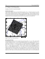
About the Cover
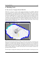
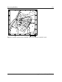
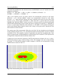
The cover picture shows a landfill in Hamburg, Germany. The deposit operated from 1935 to
1979, during the operation time it accepted municipal as well as industrial chemical wastes. The
deposit rises about 40 m above the surrounding terrain and covers an area of about 390 000 m2
(. 96 acres).
Software Licence Agreement
Software Licence Agreement
This document is a legal agreement between you, the end user and the authors. By using the
software, you are agreeing to be bound by the terms of this agreement.
Licence
You have the non-exclusive right to use the enclosed Software. You have the right to copy the
Software onto a single computer and the right for you and others to use that copy of the Software
on that single computer. You may copy the software onto computers (office, home, laptop)
provided that only one copy of the Software is used at anytime. Where the Software are copied
onto multiple computers, or is used on a network or file server, you must purchase a number of
copies of the Software equal to the number of users who will use the Software.
You may not distribute copies of the Software or documentation to others. You may not assign
sublicence, or transfer this Licence without the written permission of the authors. You may not
rent or lease the Software without the prior permission of the authors. You may not incorporate
all or part of the Software into another product for the use of other than yourself without the
written permission of the authors.
Term
This Licence is effective until terminated. You may terminate it by destroying the Software and
documentation and all copies thereof. The Licence will also terminate if you fail to comply with
any term or condition of the Licence. Upon such termination you must destroy all copies of the
Software and documentation.
Disclaimer
The user of this software accepts and uses it at his/her own risk.
The authors do not make any expressed of implied warranty of any kind with regard to this
software. Nor shall the authors be liable for incidental or consequential damages with or arising
out of the furnishing, use or performance of this software.
© Copyright 1991-1996 Wen-Hsing Chiang & Wolfgang Kinzelbach. All Rights Reserved.
Trademarks
Most computer and software brand names have trademarks or registered trademarks. The
individual trademarks have noto been listed here.
Table of Contents
Preface
1.
Introduction
What Is PMWIN
New Features in PMWIN
System Requirements
Setting Up PMWIN
Online Help
2.
Your First Groundwater Flow Model with PMWIN
The Sample Problem
Starting PMWIN
Run a Steady-State Flow Simulation
Create a Flow Model
Assign Model Data
Perform the Flow Simulation
Check Simulation Results and Produce Output
3.
The Modeling Environment
3.1
3.2
3.3
3.3.1
3.3.2
3.3.3
3.3.4
3.3.5
3.3.6
3.3.7
3.3.8
3.3.9
The Grid Editor
The Data Editor
PMWIN Menus
The File Menu
The Grid Menu
The Parameters Menu
The Packages Menu
The Source Menu
The Estimation Menu
The Value Menu
The Options Menu
The Run Menu
4.
Modeling Tools
4.1
4.1.1
4.1.2
4.1.3
4.1.4
4.2
4.3
4.4
4.5
4.6
The Advective Transport Model PMPATH
The Semi-analytical Particle Tracking Method
PMPATH Modeling Environment
PMPATH Options
PMPATH Output Files
The Field Interpolator PMDIS
The Field Generator PMFGN
The Results Extractor
The Water Balance Calculator
The Graph Viewer
5.
Applications and Sample Problems
5.1
5.2
5.3
5.4
5.5
5.6
The Theis Solution
Model Calibration with PEST
Estimation of Extraction Rates with PEST
Using the Field Interpolator
An Example of Stochastic Modeling
Simulation of a Two-Layer Aquifer System in which the Top Layer Converts between Wet
and Dry
Simulation of a Water-Table Mound Resulting from Local Recharge
Simulation of a Perched Water Table
Simulation of an Aquifer System with Irregular Recharge and a Stream
Simulation of a Flood in a River
Simulation of the Storage-Depletion
Simulation of a Non-declining Cyclical Ramp Load Problem
Two-Dimensional Transport in a Uniform Flow Field
A Field Application
5.7
5.8
5.9
5.10
5.11
5.12
5.13
5.14
Appendix
1
2
3
4
5
6
7
Limitations of PMWIN
Files and Formats
Input Instructions of MODFLOW
Input Instructions of MT3D
Using PMWIN with your MODFLOW
Running MODPATH with PMWIN
Input data files for the supported programs
References
Preface
Processing Modflow was originally developed for a remediation project of a disposal site in the
coastal region of Northern Germany several years ago. At the beginning of the work, the code
was designed as a pre- and postprocessor for MODFLOW. The size of the code grew up, as we
began to add several additional options and performances for supporting the particle tracking
code MODPATH and the solute transport program MT3D. In the mean time, various codes were
developed by numerous investigators for simulating specific features of the hydrologic system
with MODFLOW. In these days programs for the parameter estimation and model calibration,
such as PEST or MODFLOW/P, are also available.
Two years ago, we began to prepare the Windows-version of Processing Modflow with the goal
of bringing various codes together in a complete simulation system. We have prepared the
Windows-based advective transport model PMPATH and added options for supporting the codes
including MODFLOW, MODPATH, MODPATH-PLOT, MT3D and PEST. We incorporated
MODFLOW, PMPATH and the educational version of PEST and MT3D in the simulation
system. We have made efforts to explain the theory and methods used in the code and included
numerous examples to facilitate the use of Processing Modflow.
Acknowledgments
We are very grateful to John Doherty who provided the educational release of PEST, explanations
of the program parameters and many valuable comments and criticisms. We are indebted to
Chunmiao Zheng of the Department of Geology at the University of Alabama who provided the
educational release of the solute transport model MT3D and the corresponding input instructions.
Many thanks are due to many of our friends and colleagues for their contribution in developing,
checking and validating the various parts of this software.
Wen-Hsing Chiang
Wolfgang Kinzelbach
Processing Modflow
1-1
1. Introduction
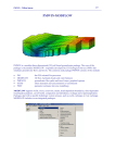
What Is PMWIN
Processing Modflow for Windows (PMWIN) is a simulation system for modeling groundwater
flow and transport processes with the modular three-dimensional finite-difference groundwater
model MODFLOW of the U. S. Geological Survey (McDonald et al., 1988), the particle tracking
model PMPATH for Windows (Chiang, 1994) or MODPATH (Pollock, 1988, 1989, 1994), the
solute transport model MT3D (Zheng, 1990) and the parameter estimation program PEST
(Doherty et al., 1994). The codes supported by PMWIN are widely used and available at nominal
cost.
The applications of MODFLOW to the description and prediction of the behavior of groundwater
systems have increased significantly over the last few years. Since the publication of MODFLOW
various codes have been developed by numerous investigators for simulating specific features of
the hydrologic system. MODFLOW can simulate the effects of wells, rivers, drains, headdependent boundaries, recharge and evapotranspiration. PMWIN also supports the calculation
of elastic and inelastic compaction of an aquifer due to changes of hydraulic heads.
The particle tracking model PMPATH for Windows is included in PMWIN. PMPATH uses a
semi-analytical particle tracking scheme (Pollock, 1988) to calculate the groundwater paths and
travel times. PMPATH allows a user to perform particle tracking with just a few clicks of the
mouse. Both forward and backward particle tracking schemes are allowed for steady-state and
transient flow fields. PMPATH calculates and shows pathlines or flowlines and travel time marks
simultaneously. It provides various on-screen graphical options including head contours,
drawdown contours and velocity vectors.
The development of the particle tracking model MODPATH can be roughly divided into two
stages. The earlier release of MODPATH was developed to compute flowlines based on output
from steady-state flow simulations by MODFLOW. The most recent release of MODPATH
permits forward and backward tracking in transient flow fields as well as steady-state flow fields.
Output from MODPATH can be displayed graphically by using the program MODPATH-PLOT.
The MT3D transport model uses a mixed Eulerian-Lagrangian approach to the solution of the
three-dimensional advective-dispersive-reactive transport equation. MT3D is based on the
assumption that changes in the concentration field will not affect the flow field significantly. This
allows the user to construct and calibrate a flow model independently. After a flow simulation is
complete, MT3D retrieves the calculated hydraulic heads and various flow terms saved by
MODFLOW. The MT3D transport model can be used to simulate changes in concentration of
single species miscible contaminants in groundwater considering advection, dispersion and some
simple chemical reactions. The chemical reactions included in the model are currently limited to
equilibrium-controlled linear or non-linear sorption and first-order irreversible decay or
biodegradation.
The purpose of PEST (which is an acronym for Parameter ESTimation) is to assist in data
Introduction
1-2
Processing Modflow
interpretation and in model calibration. If there are field or laboratory measurements, PEST can
adjust model parameters and/or excitation data in order that the discrepancies between the
pertinent model-generated numbers and the corresponding measurements are reduced to a
minimum. It does this by taking control of the model (MODFLOW) and running it as many times
as is necessary in order to determine this optimal set of parameters and/or excitations. PMWIN
helps the user to inform PEST of assigning the adjustable parameters and excitations.
New Features in PMWIN
! PMWIN is capable of using all available memory. There is almost no limit to the model size.
PMWIN can handel models with up to 80 layers and 1000 stress periods. Each model layer
can consist of 2000 × 2000 cells. Of course a sufficiently large harddisk must be avaiable to
store the forthcoming result files.
! PMWIN provides comprehensive supports to the parameter estimation program, PEST. Users
just need to define zones of parameters and send them to a Parameter List. This is all
accomplished with a click of the mouse.
! PMWIN provides a Layer Options dialog box. Transmissivity, vertical leakance and storage
coefficient of each layer can be specified by the user directly or will be calculated by applying
a particular rule, e.g., Transmissivity = Hydraulic Conductivity × Layer Thickness. The choice
for each of these parameters is accomplished by choosing between "Calculated" or "User
Specified" in the Layer Options dialog box.
! Three additional packages of MODFLOW are supported by PMWIN. They are the Horizontal
Flow Barrier Package (HFB1) for easily simulating slurry walls, the Time Variant Specified
Head Package (CHD1), and the Interbed-Storage Package (IBS1) for simulating transient
storage and calculating compaction and subsidence of an aquifer due to changes of hydraulic
heads.
! PMWIN provides a powerful Result Extractor. Normally, simulation results from Modflow
or MT3D are saved unformatted (binary) and cannot be viewed. The unformatted simulation
result files include hydraulic head, drawdown, cell-by-cell flow terms, preconsolidation head,
compaction, subsidence and concentration. The Result Extractor allows the user to extract
simulation results from any stress period, time step and layer and put them into a spread sheet.
Users can then view the results or save them in ASCII or SURFER-compatible data files.
! Using the Field Generator provided by PMWIN, fields with heterogeneously-distributed
transmissivity or hydraulic conductivity can be generated. This allows the user to statistically
simulate effects and influences of unknown small-scale heterogeneities. The Field Generator
(Frenzel, 1995) is based on Mejía's algorithm (1974).
! PMWIN can display temporal development curves of simulation results including hydraulic
heads, drawdowns, concentrations, preconsolidation heads, compaction of a model layer and
Introduction
Processing Modflow
1-3
subsidence of an entire aquifer.
! The Water Budget Calculator for calculating water budgets has been improved. It cannot only
calculate the budget of user-specified zones but also the exchange of flows between zones.
This facility is very useful in many practical cases. It allows the user to determine the flow
through a particular boundary exactly.
! PMWIN comes with the educational version of MT3D and PEST and provides numerous
examples, including the test problems of the STR1, IBS1, BCF2 and MT3D packages.
! PMWIN can create contour maps or solid fill plots of input data or simulation results. Solid
Fill can utilize the full range of RGB colors to fill cells with different values. Contours can be
added to these plots. Report-quality graphics may be saved to a wide variety of file types,
including SURFER, DXF, HPGL and BMP (Windows Bitmap).
System Requirements
Hardware
Personal computer running Microsoft Windows 3.1 or later or Windows 95
8 MB of available memory (16MB or more recommended)
One 3.5" high-density disk drive and a hard disk (complete installation requires 27MB)
EGA or higher-resolution monitor
Microsoft Mouse or compatible pointing device
Software
The models MODFLOW, MODPATH and MT3D must be compiled by Lahey Fortran F77LEM/32.
Setting Up PMWIN
You install PMWIN on your computer using the program SETUP.EXE contained in disk #1. The
Setup program installs PMWIN itself and other program components from the distribution disks
to your hard disk.
Note that you cannot simply copy files from the distribution disks to your hard disk and run
PMWIN. You must use the Setup program, which decompresses and installs the files in the
appropriate directories.
After having installed PMWIN, you should add the following entries to the file CONFIG.SYS and
AUTOEXEC.BAT and reboot your computer.
CONFIG.SYS:
FILES=80
Introduction
1-4
Processing Modflow
AUTOEXEC.BAT:
SET PESTDIR=path
where path is the subdirectory of the PEST programs. If you do not have PEST, path should be
the subdirectory of PMWIN, e.g. C:\PMWIN.
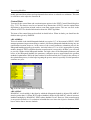
Online Help
The online help system references nearly all aspects of PMWIN. You can access Help through the
Help menu Contents command, by searching for specific topics with the Help Search tool, or by
pressing F1 to get context sensitive Help on the PMWIN modeling environment.
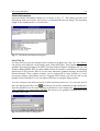
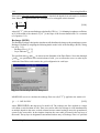
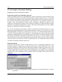
Help Search
The fastest way to find a particular topic in Help is to use the Search dialog box. To display the
Search dialog box, you can either choose Search from the Help menu or click the Search button
on any Help topic screen.
To search Help
1. From the Help menu, choose Search. (You can also choose the Search button from any Help
topic Window)
2. In the Search dialog box, type a word, or select one from the list by scrolling up or down.
Press ENTER or choose Show Topics to display a list of topics related to the word you
specified.
3. Select a topic name, and then press ENTER or choose Go To to view the topic.
Context-Sensitive Help
Many parts of PMWIN are context-sensitive. Context-sensitive means you can get Help on these
parts directly without having to go through the Help menu. For example, to get Help on any
dialog box of PMWIN, just click the Help button.
Introduction
Processing Modflow
2-1
2. Your First Groundwater Flow Model with PMWIN
It takes just a few minutes to build your first groundwater flow model with PMWIN. You create
a groundwater model by choosing New Model from the File menu. Next, you determine the size
of the model grid by choosing Mesh Size from the Grid menu. Then, you specify the geometrical
setup and assign the model parameters, such as hydraulic conductivity. Finally, you perform the
flow simulation by choosing Flow Computation (Modflow) from the Run menu. After the flow
simulation is completed, you can use the modeling tools provided by PMWIN to view the results,
to calculate water bugdets of particular zones, or graphically display the results, such as head
contours. You can also use PMPATH to calculate and save pathlines.
This chapter provides an overview of the modeling process with PMWIN, describes the basic
skills you need to use PMWIN, and takes you step by step through the sample model. A complete
reference for all menus and dialog boxes in PMWIN is contained in Chapter 3. The modeling
tools are described in Chapter 4.
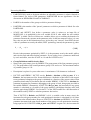
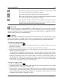
The Sample Problem
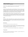
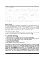
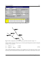
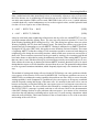
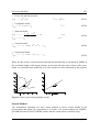
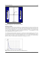
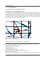
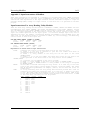
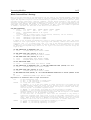
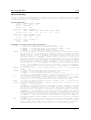
The configuration of the sample problem is shown in Fig. 2.1. The flow domain is bounded by
no-flow boundaries on the north and south sides. The west and east sides are constant-head
boundaries. The hydraulic heads on the west and east boundaries are 9 m and 8 m, respectively.
Fig. 2.1 Configuration of the sample problem
The aquifer consists of two layers. The first layer is unconfined and the second layer is confined.
Horizontal hydraulic conductivities of the first and second layers are 0.005 m/s and 0.001 m/s,
respectively. Vertical hydraulic conductivity of both layers is about 10 percent of the horizontal
hydraulic conductivity. The effective porosity is approximately 25 percent. The elevation of the
top of the first layer is 10m. The thickness of the first layer and the second layer is 13 m and 5 m,
Your First Groundwater Flow Model with PMWIN
2-2
Processing Modflow
respectively. A contaminated area lies in the first layer next to the west boundary. To clean up the
aquifer, a fully penetrating pumping well is located next to the east boundary.
A numerical model has to be developed for this site to calculate the required pumping rate of a
well. The pumping rate must be large enough, so that the contaminated area lies within the
capture zone of the pumping well. We will use PMWIN to construct the numerical model and use
PMPATH to compute the capture zone.
Starting PMWIN
When you run the PMWIN Setup program, Setup automatically creates a new program group and
new program items for Processing Modflow in Windows. You are then ready to start PMWIN
from Windows.
<
!
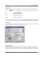
To start PMWIN from Windows
Double-click the Processing Modflow icon.
When you start PMWIN, you see the interface of PMWIN with a Menu bar and a tool bar. The
tool bar contains an Open Model icon, you can click this icon to open a model.
Run a Steady-State Flow Simulation
There are four main steps to run a steady-state flow simulation:
1. Create a flow model
2. Assign model data
3. Perform the flow simulation
4. Check simulation results and produce output
Create a Flow Model
The first step in running a flow simulation is to create a new model.
<
1.
2.
To create a flow model
Choose New Model from the File menu. A New Model dialog box will appear. Select a
directory for saving the model data, such as C:\PMWIN\EXAMPLES\SAMPLE, and type
the file name SAMPLE for the sample model. A PMWIN model must always have the file
extension MDL. It is a good idea to save every model in a separate directory, where the
model and its output data will be kept. This will also allow you to run several models
simultaneously (multitasking). If a desired directory for saving a new model is not available,
you have to use the File Manager of Windows or other utilities to create the directory.
Click OK.
PMWIN takes only a few seconds to create the new model and show the model name on the
title bar.
Your First Groundwater Flow Model with PMWIN
Processing Modflow
2-3
Assign Model Data
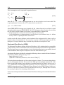
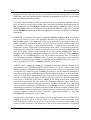
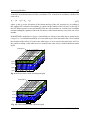
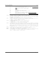
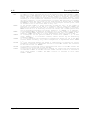
The second step in running a flow simulation is to generate the model grid (mesh), specify
boundary conditions, and assign model parameters to the model grid. In MODFLOW, an aquifer
system is replaced by a discretized domain consisting of an array of nodes and associated finite
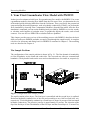
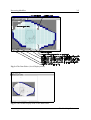
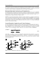
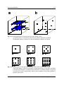
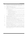
difference blocks (cells). Fig. 2.2 shows a spatial discretization of an aquifer system with a mesh
of cells and nodes at which hydraulic heads are calculated. The nodal grid forms the framework
of the numerical model. Hydrostratigraphic units can be represented by one or more model layers.
The thicknesses of each model cell and the width of each column and row may be variable. The
locations of cells are described in terms of columns, rows, and layers. PMWIN uses an index
notation [J, I, K] for locating the cells. For example, the cell located in the 2nd column, 6th row,
and the first layer is denoted by [2, 6, 1].
Fig. 2.2 Spatial discretization of an aquifer system and the cell indices
<
1.
2.
3.
4.
To generate the model grid
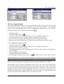
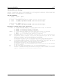
Choose Mesh Size from the Grid menu.
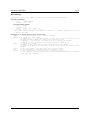
A Model Dimension dialog box will come up (Fig. 2.3)
Type 2 for the number of layers, 30 for the numbers of columns and rows, and 20 for the size
of columns and rows.
Click OK.
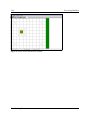
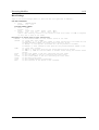
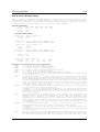
PMWIN changes the pull-down menus and shows the generated model grid (Fig. 2.4). Some
menus items are dimmed, as they will not be used here. PMWIN allows you to shift or rotate
the model grid, change the width of each model column or row, or add or delete model
columns or rows. For our sample problem, you do not need to modify the model grid. See
section 3.1 for more information about the Grid Editor.
Choose Leave Editor from the File menu or click the Leave Editor icon
Your First Groundwater Flow Model with PMWIN
2-4
Processing Modflow
Fig. 2.3 The Model Dimension dialog box
Fig. 2.4 The generated model grid
The next step is to specify the type of layers.
<
1.
2.
3.
4.
To assign the type of layers
Choose Layer Type from the Grid menu.
A Layer Options dialog box will appear.
Clicking a cell of the Type column, a drop-down button will appear in the current cell. If you
click on the button, a list will drop down which contains all the possible layer types, as shown
in Fig. 2.5.
Select type 1 for the first layer and type 0 for the second layer.
Click OK.
Your First Groundwater Flow Model with PMWIN
Processing Modflow
2-5
Fig. 2.5 The Layer Options dialog box and the layer type drop-down list
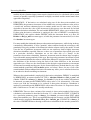
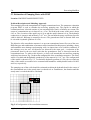
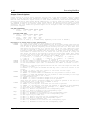
Now, you will specify boundary conditions of the flow model by using the IBOUND array. This
array contains a code for each model cell which indicates whether (1) the hydraulic head is
computed (active variable-head cell or active cell), (2) the hydraulic head is kept fixed at a given
value (constant-head cell or time-varying specified-head cell), or (3) no flow takes place within
the cell (inactive cell). It is suggested to use 1 for an active cell, -1 for a constant-head cell, and
0 for an inactive cell.
For the sample problem, we need to assign -1 to the cells on the west and east boundaries and 1
to all other cells.
<
1.
2.
3.
4.
5.
6.
To assign the boundary condition to the flow model
Choose Boundary Condition < IBOUND (Modflow) from the Grid Menu.
PMWIN shows the top view of the model grid (Fig. 2.6). The grid cursor is located in the
cell [1, 1, 1], that is the upper-left cell of the first layer. The value of the current cell is shown
at the bottom of the status bar. The default value of the IBOUND array is 1. The grid cursor
can be moved horizontally by using the arrow keys or by clicking the mouse on the desired
position. To move to an other layer, you can use PgUp or PgDn keys or click the edit field
in the tool bar, type the new layer number, and then press enter.
Pressing the right mouse button, PMWIN shows a Cell Value dialog box.
Type -1 in the dialog box, then click OK.
The upper-left cell of the model has been specified as a constant-head cell.
Now turn Duplication on by clicking the Duplication icon
.
The small box on the lower-right corner of this icon will be highlighted. The current cell
value will be duplicated to all cells passed by the grid cursor, if it is moved while Duplication
is on. You can turn Duplication off by clicking the Duplication icon again.
Move the grid cursor from the upper-left cell [1, 1, 1] to the lower-left cell [1, 30, 1] of the
model grid.
The value of -1 is duplicated to all cells on the west side of the model.
Move the grid cursor to the upper-right cell [30, 1, 1].
Your First Groundwater Flow Model with PMWIN
2-6
Processing Modflow
7.
Move the grid cursor from the upper-right cell [30, 1, 1] to the lower-right cell [30, 30, 1].
The value of -1 is duplicated to all cells on the east side of the model.
8. Turn Layer Copy on by clicking the Layer Copy icon .
The small box on the lower-right corner of this icon will be highlighted. The cell values of
the current layer will be copied to other layers, if you move to the other model layer while
Layer Copy is on. You can turn Layer Copy off by clicking the Layer Copy icon.
9. Move to the second layer.
The cell values of the first layer are copied to the second layer.
10. Choose Leave Editor from the File menu or click the Leave Editor icon
Fig. 2.6 Top view of the model grid. Model data are assigned to each
cell in each layer.
The next step is to specify the geometrical setup of the model.
< To specify the elevation of the top of model layers
1. Choose Top of Layers (TOP) from the Grid menu.
PMWIN shows the model grid.
2. Choose Matrix<Reset from the Value menu (or press Ctrl+R).
A Reset Matrix dialog box will come up.
3. Type 10 in the dialog box, then click OK.
The elevation of the top of the first layer is set to 10.
4. Move to the second layer by pressing PgDn.
5. Repeat steps 2 and 3 to set the top of the second layer to -3.
6. Choose Leave Editor from the File menu or click the Leave Editor icon
<
1.
To specify the elevation of the bottom of model layers
Choose Bottom of Layers (BOT) from the Grid menu.
Your First Groundwater Flow Model with PMWIN
Processing Modflow
2.
3.
2-7
Repeat the same procedure as described above to set the bottom of the first layer to -3 and
the bottom of the second layer to -8.
Choose Leave Editor from the File menu or click the Leave Editor icon
Now, we are going to specify the temporal and spatial parameters of the model. For the sample
problem, spatial parameters include the starting hydraulic head, horizontal and vertical hydraulic
conductivities, and effective porosity.
<
1.
2.
<
1.
To specify the temporal parameters
Choose Time from the Parameters menu.
A Time Parameters dialog box will come up. The temporal parameters include the time unit
and the numbers of stress periods, time steps and transport steps. In MODFLOW, the
simulation time is divided into stress periods - i.e., time intervals during which all external
excitations or stresses are constant - which are, in turn, divided into time steps. In the MT3D
model, each time step is further divided into smaller time increments, called transport steps.
The length of stress periods is not relevant to a steady state flow simulation. However, if you
want to perform contaminant transport simulation with MT3D at a later time, you must
specify the actual time length in the table.
Click OK to accept the default values.
9.
To specify the initial hydraulic head
Choose Starting Values<Hydraulic Heads from the Parameters menu.
PMWIN shows the model grid. Now, you can specify the initial hydraulic heads for each
model cell. The initial hydraulic head at a constant-head boundary will be kept constant
during the flow simulation.
Choose Matrix<Reset from the Value menu (or press Ctrl+R) and type 8 in the dialog box,
then click OK.
Move the grid cursor to the upper-left model cell.
Press the right mouse button and type 9 in the Cell Value dialog box, then click OK.
Now turn Duplication on by clicking the Duplication icon
.
The small box on the lower-right corner of this icon will be highlighted. The current cell
value will be duplicated to all cells passed by the grid cursor, if it is moved while Duplication
is on.
Move the grid cursor from the upper-left cell to the lower-left cell of the model grid.
The value of 9 is duplicated to all cells on the west side of the model.
Turn Layer Copy on by clicking the Layer Copy icon .
The small box on the lower-right corner of this icon will be highlighted. The cell values of
the current layer will be copied to another layer, if you move to the other model layer while
Layer Copy is on.
Move to the second layer by pressing PgDn.
The cell values of the first layer are copied to the second layer.
Choose Leave Editor from the File menu or click the Leave Editor icon
<
1.
To specify the horizontal hydraulic conductivity
Choose Horizontal Hydraulic Conductivity from the Parameters menu.
2.
3.
4.
5.
6.
7.
8.
Your First Groundwater Flow Model with PMWIN
2-8
2.
3.
4.
5.
<
1.
2.
3.
4.
5.
<
1.
2.
3.
4.
5.
Processing Modflow
Choose Matrix<Reset from the Value menu (or press Ctrl+R) and type 0.005 in the dialog
box, then click OK.
Move to the second layer by pressing PgDn.
Choose Matrix<Reset from the Value menu (or press Ctrl+R) and type 0.001 in the dialog
box, then click OK.
Choose Leave Editor from the File menu or click the Leave Editor icon
To specify the vertical hydraulic conductivity
Choose Vertical Hydraulic Conductivity from the Parameters menu.
Choose Matrix<Reset from the Value menu (or press Ctrl+R) and type 0.0005 in the dialog
box, then click OK.
Move to the second layer by pressing PgDn.
Choose Matrix<Reset from the Value menu (or press Ctrl+R) and type 0.0001 in the dialog
box, then click OK.
Choose Leave Editor from the File menu or click the Leave Editor icon
To specify the effective porosity
Choose Effective Porosity from the Parameters menu.
Choose Matrix<Reset from the Value menu (or press Ctrl+R) and type 0.25 in the dialog
box, then click OK.
Turn Layer Copy on by clicking the Layer Copy icon .
Move to the second layer by pressing PgDn.
Choose Leave Editor from the File menu or click the Leave Editor icon
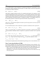
The last step before performing the flow simulation of the sample model is to specify the location
of the pumping well and its pumping rate. In MODFLOW, an injection or pumping well is
represented by a node (or a cell). The user specifies an injection or pumping rate for each node.
It is implicitly assumed that the well penetrates the full thickness of the cell. MODFLOW can
simulate the effects of pumping from a well that penetrates more than one aquifer or layer
provided that the user supplies the pumping rate for each layer. The total pumping rate for the
multilayer well is equal to the sum of the pumping rates from the individual layers. The pumping
rate for each layer ( Qk ) can be approximately calculated by dividing the total pumping rate
( Qtotal ) in proportion to the layer transmissivities (McDonald and Harbaugh, 1988):
Q k ' Qtotal @
Tk
ET
(2.1)
where Tk is the transmissivity of layer k and ET is the sum of the transmissivities of all layers
penetrated by the multilayer well.
As we do not know the required pumping rate for capturing the contaminated area shown in
Fig. 2.1, we will try a total pumping rate of 0.02 m3/s. By applying equation 2.1, the pumping
rates are 0.0185 m3/s and 0.0015 m3/s in the first and second layer, respectively.
Your First Groundwater Flow Model with PMWIN
Processing Modflow
<
1.
2.
3.
4.
5.
6.
2-9
To specify the pumping well and the pumping rate
Choose Well (WEL1) from the Packages menu.
Move the grid cursor to the cell [25, 15, 1]
Press the right mouse button and type -0.0185, then click OK. Negative value is used to
indicate a pumping well.
Move to the second layer by pressing PgDn.
Press the right mouse button and type -0.0015, then click OK.
Choose Leave Editor from the File menu or click the Leave Editor icon
Perform the Flow Simulation
Now everything is ready to run the flow simulation with MODFLOW.
<
1.
2.
To perform the flow simulation
Select Run Menu and Choose Flow Computation (Modflow).
A Run Modflow dialog box will appear (Fig. 2.7).
Click OK to start the flow computation.
Prior to running MODFLOW, PMWIN will use user-specified data to generate input files of
MODFLOW and MODPATH as listed in the table of the Run Modflow dialog box. An input
file will be generated, only if the Generate flag is set to YES. You can click on a row to
toggle the Generate flag between YES and No. Generally, you do not need to change the
Generate flags, as PMWIN will care about the settings.
Fig. 2.7 The Run Modflow dialog box
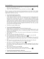
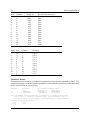
Check Simulation Results and Produce Output
During a flow simulation, MODFLOW writes a detailed run record to the file
path\OUTPUT.DAT, where path is the directory in which your model data are saved. If a flow
simulation is successfully complete, MODFLOW saves the simulation results in various
unformatted (binary) files as listed in Table 2.1. Prior to running MODFLOW, the user may
Your First Groundwater Flow Model with PMWIN
2-10
Processing Modflow
control the output of these unformatted (binary) files by choosing Output Control<Modflow from
the Packages menu. The output file path\INTERBED.DAT will only be generated, if the Interbed
Storage Package is activated (see Chapter 3 for details about the Interbed Storage Package).
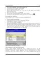
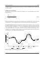
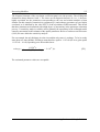
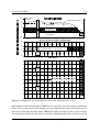
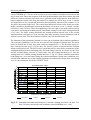
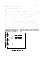
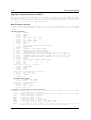
For checking the simulation results, MODFLOW calculates a volumetric water budget for the
entire model at the end of each time step, and saves it in the record file (see Fig. 2.8). A water
budget provides an indication of the overall acceptability of the numerical solution. In numerical
solution techniques, the system of equations solved by a model actually consists of a flow
continuity statement for each model cell. Continuity should also exist for the total flows into and
out of the entire model or a sub-region. This means that the difference between total inflow and
total outflow should equal the total change in storage. It is recommended to read the record file
or at least glance at it. The record file contains other further essential information. In case of
difficulties, this supplementary information could be very helpful.
File
Contents
path\OUTPUT.DAT
Detailed run record and simulation report
path\HEADS.DAT
Hydraulic heads
path\DDOWN.DAT
Drawdowns, the difference between the starting heads and
the calculated hydraulic heads.
path\BUDGET.DAT
Cell-by-Cell flow terms
path\INTERBED.DAT
Subsidence of the entire aquifer and compaction and
preconsolidation heads in individual layers.
Table 2.1 Output files from MODFLOW
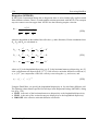
VOLUMETRIC BUDGET FOR ENTIRE MODEL AT END OF TIME STEP 1 IN STRESS PERIOD 1
----------------------------------------------------------------------------CUMULATIVE VOLUMES
L**3/T
RATES FOR THIS TIME STEP
L**3/T
----------------------------------------IN:
--STORAGE =
CONSTANT HEAD =
WELLS =
TOTAL IN =
OUT:
---STORAGE =
CONSTANT HEAD =
WELLS =
TOTAL OUT =
IN - OUT =
0.00000
0.68083E-01
0.00000
0.68083E-01
IN:
--STORAGE =
CONSTANT HEAD =
WELLS =
TOTAL IN =
0.00000
0.68083E-01
0.00000
0.68083E-01
0.00000
0.48096E-01
0.2E-01
0.68096E-01
-0.13150E-04
OUT:
---STORAGE =
CONSTANT HEAD =
WELLS =
TOTAL OUT =
IN - OUT =
0.00000
0.48096E-01
0.20000E-01
0.68096E-01
-0.13150E-04
PERCENT DISCREPANCY =
-0.02
PERCENT DISCREPANCY = -0.02
Fig. 2.8 Volumetric budget for the entire model written by MODFLOW
There are situations in which it is useful to calculate flow terms for various subregions of the
model. To facilitate such calculations, flow terms for individual cells are saved in the file
Your First Groundwater Flow Model with PMWIN
Processing Modflow
2-11
path\BUDGET.DAT. These individual cell flows are referred to as cell-by-cell flow terms, and
are of four types: (1) cell-by-cell stress flows, or flows into or from an individual cell due to one
of the external stresses (excitations) represented in the model, e.g., pumping well or recharge;
(2) cell-by-cell storage terms, which give the rate of accumulation or depletion of storage in an
individual cell; (3) cell-by-cell constant-head flow terms, which give the net flow to or from
individual constant-head cells; and (4) internal cell-by-cell flows, which are the flows across
individual cell faces-that is, between adjacent model cells. The Water Budget Calculator uses the
cell-by-cell flow terms to compute water budgets for the entire model, user-specified subregions,
and flows between adjacent subregions. PMPATH uses the cell-by-cell flow terms and calculated
hydraulic heads for calculating and displaying pathlines.
In addition to the Water Budget Calculator and PMPATH, PMWIN provides various possibilities
for checking simulation results and creating graphical output. Using the Results Extractor,
simulation results of any layer and time step can be read from the unformatted (binary) result files
and saved in ASCII Matrix files. An ASCII Matrix file contains a value for each model cell in a
layer. The format of the ASCII Matrix file is described in Appendix 2. PMWIN can generate
contour maps based on an ASCII Matrix file.
In the following, we will accomplish the steps:
1. Use the Water Budget Calculator to compute water budgets of each layer and the entire
model, and check if the percent discrepancies of in- and outflows are acceptable small.
2. Use the Result Extractor to read and save the calculated hydraulic heads of each layer.
3. Generate contour maps based on the calculated hydraulic heads saved in step 2.
4. Create a solid fill plot based on the calculated hydraulic heads saved in step 2 and add
contours to the plot.
5. Use PMPATH to produce pathlines as well as the capture zone of the pumping well.
<
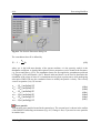
1.
2.
3.
4.
5.
6.
7.
To calculate subregional water budgets
Choose Water Budget from the Run menu.
A Water Budget dialog box will come up (Fig. 2.9). For a steady-state flow simulation, you
do not need to change the settings in the Time group.
Click Zones.
A zone is a subregion of a model for which a water budget will be calculated. A zone is
indicated by a zone number ranging from 0 to 50. A zone number must be assigned to each
model cell. The zone number 0 shows that a cell is not associated with any zone. Follow the
steps 3 to 5 to assign zone numbers 1 to the first and 2 to the second layer.
Choose Matrix<Reset from the Value menu (or press Ctrl+R), type 1 in the dialog box, then
click OK.
Press PgDn to move to the second layer.
Choose Matrix<Reset from the Value menu (or press Ctrl+R), type 2 in the dialog box, then
click OK.
Choose Leave Editor from the File menu or click the Leave Editor icon
Click OK in the Water Budget dialog box.
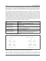
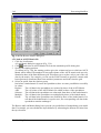
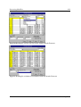
PMWIN calculates and saves the flows in the file path\WATERBDG.DAT as shown in Fig. 2.10.
Your First Groundwater Flow Model with PMWIN
2-12
Processing Modflow
The unit of the flows is [L3/T]. Flows are considered "IN", if they are entering a zone. Flows
between subregions are given in a flow matrix.
Water budgets are calculated for each zone in each layer and each time step. HORIZ.
EXCHANGE gives the flows which flow horizontally across a zone's boundary. EXCHANGE
(UPPER) or EXCHANGE (LOWER) give the flows which come from or go to the upper or
lower adjacent layers. Consider ZONE = 1 and LAYER = 1: the flow IN = 1.5266858@10-4 m3/s
of EXCHANGE (LOWER) flows from the second layer into zone #1 and flow
OUT = 3.6502272@10-4 m3/s leaves zone #1 and flows to the second layer.
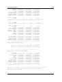
The percent discrepancy is calculated by
100 @ (IN & OUT)
(IN % OUT) / 2
(2.2)
In this example, the percent discrepancies of in- and outflows for the model and each zone in each
layer are acceptably small. This means the model equations are correctly solved.
Fig. 2.9 The Water Budget dialog box
-------------------------------------------------------PMWBLF (SUBREGIONAL WATER BUDGET) RUN RECORD
-------------------------------------------------------FLOWS ARE CONSIDERED "IN" IF THEY ARE ENTERING A SUBREGION
THE UNIT OF THE FLOWS IS [L^3/T]
TIME STEP
ZONE=
1 OF STRESS PERIOD
1 LAYER=
FLOW TERM
STORAGE
CONSTANT HEAD
HORIZ. EXCHANGE
EXCHANGE (UPPER)
EXCHANGE (LOWER)
WELLS
1
1
IN
0.0000000E+00
6.2836841E-02
0.0000000E+00
0.0000000E+00
1.5266858E-04
0.0000000E+00
OUT
IN-OUT
0.0000000E+00 0.0000000E+00
4.4093262E-02 1.8743578E-02
0.0000000E+00 0.0000000E+00
0.0000000E+00 0.0000000E+00
3.6502272E-04 -2.1235413E-04
1.8500000E-02 -1.8500000E-02
Fig. 2.10 Output from the Water Budget Calculator
Your First Groundwater Flow Model with PMWIN
Processing Modflow
DRAINS
RECHARGE
ET
RIVER LEAKAGE
HEAD DEP BOUNDS
STREAM LEAKAGE
INTERBED STORAGE
SUM OF THE LAYER
2-13
0.0000000E+00
0.0000000E+00
0.0000000E+00
0.0000000E+00
0.0000000E+00
0.0000000E+00
0.0000000E+00
6.2989511E-02
0.0000000E+00
0.0000000E+00
0.0000000E+00
0.0000000E+00
0.0000000E+00
0.0000000E+00
0.0000000E+00
6.2958285E-02
0.0000000E+00
0.0000000E+00
0.0000000E+00
0.0000000E+00
0.0000000E+00
0.0000000E+00
0.0000000E+00
3.1225383E-05
ZONE=
1 LAYER= 2
FLOW TERM
IN
OUT
IN-OUT
(all flow terms are zero, because zone 1 lies only in the first layer)
-------------------------------------------------------------ZONE=
2 LAYER= 1
FLOW TERM
IN
OUT
IN-OUT
(all flow terms are zero, because zone 2 lies only in the second layer)
ZONE=
2 LAYER=
FLOW TERM
STORAGE
CONSTANT HEAD
HORIZ. EXCHANGE
EXCHANGE (UPPER)
EXCHANGE (LOWER)
WELLS
DRAINS
RECHARGE
ET
2
IN
0.0000000E+00
5.2456958E-03
0.0000000E+00
3.6502272E-04
0.0000000E+00
0.0000000E+00
0.0000000E+00
0.0000000E+00
0.0000000E+00
OUT
IN-OUT
0.0000000E+00 0.0000000E+00
4.0024151E-03 1.2432807E-03
0.0000000E+00 0.0000000E+00
1.5266858E-04 2.1235413E-04
0.0000000E+00 0.0000000E+00
1.5000000E-03 -1.5000000E-03
0.0000000E+00 0.0000000E+00
0.0000000E+00 0.0000000E+00
0.0000000E+00 0.0000000E+00
RIVER LEAKAGE 0.0000000E+00 0.0000000E+00 0.0000000E+00
HEAD DEP BOUNDS 0.0000000E+00 0.0000000E+00 0.0000000E+00
STREAM LEAKAGE 0.0000000E+00 0.0000000E+00 0.0000000E+00
INTERBED STORAGE 0.0000000E+00 0.0000000E+00 0.0000000E+00
SUM OF THE LAYER 5.6107184E-03 5.6550838E-03 -4.4365413E-05
-------------------------------------------------------------WATER BUDGET OF SELECTED ZONES:
ZONE(
ZONE(
1):
2):
IN
6.2989511E-02
5.6107184E-03
OUT
IN-OUT
6.2958285E-02 3.1225383E-05
5.6550838E-03 -4.4365413E-05
-------------------------------------------------------------WATER BUDGET OF THE WHOLE MODEL DOMAIN:
FLOW TERM
IN
OUT
IN-OUT
STORAGE 0.0000000E+00 0.0000000E+00 0.0000000E+00
CONSTANT HEAD 6.8082534E-02 4.8095688E-02 1.9986846E-02
WELLS 0.0000000E+00 2.0000000E-02 -2.0000000E-02
DRAINS 0.0000000E+00 0.0000000E+00 0.0000000E+00
RECHARGE 0.0000000E+00 0.0000000E+00 0.0000000E+00
ET 0.0000000E+00 0.0000000E+00 0.0000000E+00
RIVER LEAKAGE 0.0000000E+00 0.0000000E+00 0.0000000E+00
HEAD DEP BOUNDS 0.0000000E+00 0.0000000E+00 0.0000000E+00
STREAM LEAKAGE 0.0000000E+00 0.0000000E+00 0.0000000E+00
INTERBED STORAGE 0.0000000E+00 0.0000000E+00 0.0000000E+00
-------------------------------------------------------------SUM 6.8082534E-02 6.8095684E-02 -1.3150275E-05
DISCREPANCY [%] -0.02
The value of the element (i,j) of the following flow matrix gives the flow
rate from the i-th zone into the j-th zone. Where i is the column
index and j is the row index.
Your First Groundwater Flow Model with PMWIN
2-14
Processing Modflow
FLOW MATRIX:
1
2
.............................
0 1
0.0000
1.5267E-04
0 2
3.6502E-04 0.0000
Fig. 2.10 (continued) Output from the Water Budget Calculator
<
1.
2.
3.
4.
5.
6.
7.
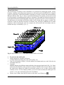
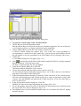
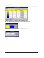
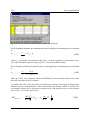
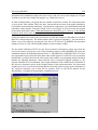
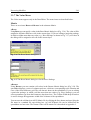
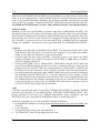
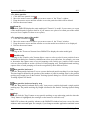
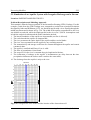
To read and save the calculated hydraulic heads of each layer
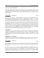
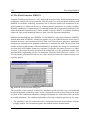
Choose Result Extractor from the Run menu.
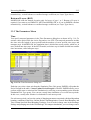
A Result Extractor dialog box appears (Fig. 2.11). You can choose a result type from the
Result Type drop-down box. In the Time/Layer group, you can specify the number of the
layer, stress period and time step from which the result should be read. The spreadsheet
displays a series of columns and rows. The intersection of a row and column is a cell. Each
cell of the spreadsheet is corresponding to a model cell in a layer. By setting the Save Format
option, the result can be optionally saved in an ASCII Matrix or a SURFER data file format.
Follow steps 2 to 6 to save the hydraulic heads of the first and second layers in two ASCII
Matrix files H1.DAT and H2.DAT.
Choose Hydraulic Head from the Result Type drop-down box.
In the Time/Layer group, type 1 in the Layer edit field.
For the sample problem, the stress period and time step number should be 1.
Click Read.
Hydraulic heads in the first layer at time step 1 and stress period 1 will be read and put into
the spreadsheet. You can scroll the spreadsheet by clicking on the scrolling bars next to the
spreadsheet.
Click Save.
A Save Matrix As dialog box will come up. Specify the file name H1.DAT and select a
directory in which H1.DAT should be saved. Click OK when ready.
Type 2 in the Layer edit field and repeat steps 4 and 5 to save the hydraulic heads of the
second layer in the file H2.DAT.
Click Close to close the dialog box.
Your First Groundwater Flow Model with PMWIN
Processing Modflow
2-15
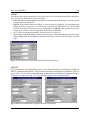
Fig. 2.11 Result types and the Results Extractor dialog box.
<
1.
To generate contour maps of the calculated heads
Choose Recycle from the Parameters menu
Data specified in Recycle will not be used by any simulation programs. We can use Recycle
to save temporary data or to display simulation results graphically.
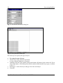
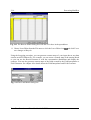
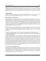
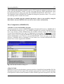
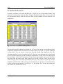
2. Choose Matrix<Browse from the Value menu (or Press Ctrl+B).
A Browse Matrix dialog box appears (Fig. 2.12). Each cell of the spreadsheet is
corresponding to a model cell in the current layer. You can load an ASCII Matrix file into
the spreadsheet or save the spreadsheet in an ASCII Matrix file by clicking Load or Save.
3. Click Load.
A Load Matrix dialog box will appear (Fig. 2.13).
4. Click
and select the file H1.DAT which will be loaded (H1.DAT is saved by using the
Results Extractor). Click OK when ready.
H1.DAT is loaded and put into the spreadsheet.
5. In the Browse Matrix dialog box, click OK.
The Browse Matrix dialog box will be closed.
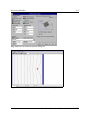
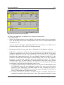
6. Choose Environment from the Options menu (or Press Ctrl+E).
An Environment Options dialog box appears (Fig. 2.14). It allows the user to modify the
appearance and position of the model grid.
7. In the Environment Options dialog box, check the Visible check box of the Contours group,
click the color button next to the Visible check box to select an appearance color of the
contours. Note that PMWIN will uncheck the Visible check box, if you leave the Editor or
move to other layers.
8. In the Environment Options dialog box, Click OK.
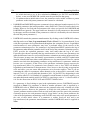
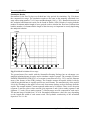
PMWIN will redraw the model and display the contours (Fig. 2.15).
9. To save the graphics, choose Save Plot As from the File menu and specify a plot format and
file name in the Save Plot As dialog box (Fig. 2.16).
10. Press PgDn to move to the second layer. Repeat steps 2 to 9 to load the file H2.DAT, display
and save the plot.
Your First Groundwater Flow Model with PMWIN
2-16
Processing Modflow
Fig. 2.12 The Browse Matrix dialog box with the cell values in the spreadsheet
11. Choose Leave Editor from the File menu or click the Leave Editor icon
save changes to Recycle.
and click Yes to
Using the foregoing procedure, you can generate contour maps of your input data or any data
saved as an ASCII Matrix file. For example, you can create a contour map of the starting heads
or you can use the Result Extractor to read the concentration distribution and display the
contours. You can also generate contour maps of the fields created by the Field Interpolator or
Field Generator. See chapter 4 for details about the Field Interpolator and Field Generator.
Fig. 2.13 The Load Matrix dialog box
Your First Groundwater Flow Model with PMWIN
Processing Modflow
2-17
Fig. 2.14 The Environment Options dialog box
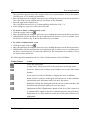
Fig. 2.15 A contour map of the hydraulic heads in the first layer
Your First Groundwater Flow Model with PMWIN
2-18
Processing Modflow
Fig. 2.16 The Save Plot As dialog box for saving graphics in different formats
<
1.
2.
3.
4.
5.
6.
7.
8.
9.
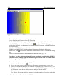
To create solid fill plots
Choose Recycle from the Parameters menu
Data specified in Recycle will not be used by any simulation programs. We can use Recycle
to save temporary data or to display simulation results graphically.
Repeat steps 2 to 5 of the foregoing procedure to load H1.DAT into the model grid. Skip
these steps, if the data were saved in the previous procedure.
Choose Search and Modify from the Value menu.
The Search and Modify dialog box appears (Fig. 2.17). If a row of the table is active, model
cells with values located between the Minimum and Maximum will be filled with the userspecified Color.
Set the first 10 rows to active by clicking on cells of the Active-column.
A row is active, if Active is set to Yes.
To assign colors to the active rows, click Spectrum.
The Color Spectrum dialog box appears (Fig. 2.18).
In the Color Spectrum dialog box, click on the Minimum button and select a color. Click on
the Maximum button and select a color. Click OK, when finished.
To set the search ranges, click Level.
The Search Level dialog box appears (Fig. 2.19).
In the Search Level dialog box, type 8 and 9 in the Minimum and Maximum edit fields. Click
OK when ready.
In the Search And Modify dialog box, click OK.
PMWIN redraws the model and fills colors to cells.
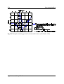
You can overlay contours to the solid fill plot by doing the following
1. Choose Environment from the Options menu, check the Visible check box, then click OK.
2. Choose Search and Modify from the Value menu, then Click OK.
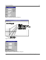
Fig. 2.20 shows a solid fill plot with contour lines.
Your First Groundwater Flow Model with PMWIN
Processing Modflow
2-19
Fig. 2.17 The Search And Modify dialog box for creating solid fill plots
Fig. 2.18 The Color Spectrum dialog box for assigning colors
Fig. 2.19 The Search Level dialog box
Your First Groundwater Flow Model with PMWIN
2-20
Processing Modflow
Fig. 2.20 Solid fill plot and contour lines
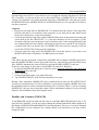
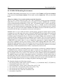
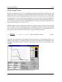
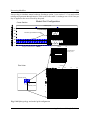
< To calculate the capture zone of the pumping well
1. Choose Pathlines and Contours from the Run menu.
The Run PMPATH dialog box appears (Fig. 2.21). You can specify the full path and filename
of the PMPATH program in the edit field, or click
. to select the PMPATH program from
a dialog box. Normally, you do not need to select the PMPATH program, as PMWIN will set
this automatically.
2. In the Run PMPATH dialog box, click OK.
PMWIN calls PMPATH by using the path and filename specified in the dialog box.
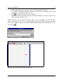
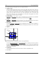
3. In PMPATH, click
and select the model file SAMPLE.MDL from the Open Model dialog
box.
PMPATH loads the SAMPLE model and shows the model grid (Fig. 2.22).
Note that if you have subsequently modified and calculated a model within PMWIN,
you must load the modified model into PMPATH again to ensure that the modifications
can be recognized by PMPATH.
4. To calculate the capture zone of the pumping well:
a. Click the Set Particle button
b. Move the mouse cursor to the model area. The mouse cursor becomes a cross hair.
c. Place the cross hair at the upper-left corner of the pumping well, as shown in Fig. 2.22.
d. Drag the cross hair until the window covers the pumping well. (Dragging means holding
the left mouse button down while you move an object with the mouse).
e. Release the mouse button.
The Particle Placement dialog box appears. Assign the numbers of particles to the edit
Your First Groundwater Flow Model with PMWIN
Processing Modflow
2-21
fields in the dialog box as shown in Fig. 2.23. When finished, click OK.
f. To set particles around the pumping well in the second layer, press PgDn to move to the
second layer and repeat the steps c, d and e.
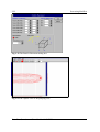
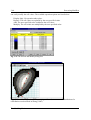
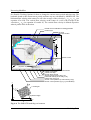
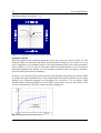
g. Click
to start the backward particle tracking.
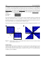
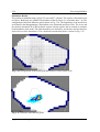
PMPATH calculates and shows the projections of the pathlines as well as the capture zone
of the pumping well (Fig. 2.24).
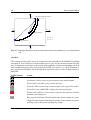
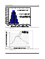
PMPATH allows you to create time-related capture zones of pumping wells. The 100-dayscapture zone shown in Fig. 2.26 is created by putting particles around the pumping well in the
second layer, using the settings in the Particle Tracking Options dialog box as shown in Fig. 2.25,
and clicking .
Fig. 2.21 The Run PMPATH dialog box
Fig. 2.22 The sample model loaded in PMPATH
Your First Groundwater Flow Model with PMWIN
2-22
Fig. 2.23 The Particle Placement dialog box
Fig. 2.24 The capture zone of the pumping well
Your First Groundwater Flow Model with PMWIN
Processing Modflow
Processing Modflow
2-23
Fig. 2.25 Particle tracking options
Fig. 2.26 100-days-capture zone calculated by PMPATH
Your First Groundwater Flow Model with PMWIN
Processing Modflow
3-1
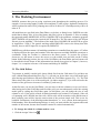
3. The Modeling Environment
PMWIN assumes that you are using consistent units throughout the modeling process. For
example, if you are using length [L] units of feet and time [T] units of days, hydraulic conductivity
will be expressed in units of ft/d, pumping rates will be in units of ft3/d and dispersivity will be in
units of ft.
All model data are specified in the Data Editor (see below) or dialog boxes. PMWIN saves the
model data in binary files. A list of the binary data files is given in Appendix 2. Prior to running
the supported models MODFLOW, MT3D or MODPATH or the parameter estimation program
PEST, PMWIN will generate the required ASCII input files. The file names of the ASCII input
files are given in Appendix 7. The formats of the input files of MODFLOW and MT3D are given
in Appendices 3 and 4. The particle tracking model PMPATH retrieves the binary data files
directly, thus no ASCII input file is required by PMPATH.
PMWIN uses pull-down menus. All modeling operations are controlled from the menu. A Toolbar
is displayed below the menu and contains icons that represent available PMWIN operations or
commands. Using the Toolbar is a shortcut to the menu system. To execute one of these
shortcuts, use the mouse to move the cursor over the toolbar icon and click on the Toolbar
button. In the following sections, the use of the Grid Editor, the Data Editor and each menu will
be described in detail. Some of this information has already been given in Chapter 2, however,
chapter 3 is a complete reference of all menus and dialogs in PMWIN.
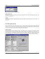
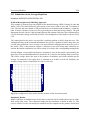
3.1 The Grid Editor
To generate or modify a model grid, choose Mesh Size from the Grid menu. If a grid does not
exist, a Model Dimension dialog box (Fig. 3.1) will ask you for the basic size of the model grid.
After having specified these data and clicked OK, the Grid Editor appears (Fig. 3.2). The Grid
Editor shows the plan view of the model grid. An index notation [J, I] is used to describe the
location of the grid cursor in terms of columns [J] and rows [I].
At the first time you use the Grid Editor, you can insert or delete columns or rows (see below).
After having leaved the Grid Editor and saved the grid, you can subsequently refine the existing
model grid by calling the Grid Editor again. In each phase, you can change the size of each
column or row. If the grid is refined, all model parameters are retained. For example, if the cell
of a pumping well is divided into four cells, all four cells will be treated as wells and the sum of
their pumping rates will be kept the same as that of the previous single well. This is true for
hydraulic conductance of the head-dependent boundaries, i.e., river, stream, drain and generalhead boundary. If the Stream-Routing Package is used, you must redefine the segment and reach
number of the stream, because these number cannot be retained automatically.
< To change the width of a column and/or a row
1. Click the Assign Value icon
The Modeling Environment
3-2
Processing Modflow
The grid cursor appears only if the Assign Value icon is pressed down. You do not need to
click this icon, if it is already pressed down.
2. Move the grid cursor by using the arrow keys or by clicking the mouse on the desired position.
The sizes of the current column and row are shown on the Statusbar.
3. Press the right mouse button once.
The Grid Editor shows a Size of Column and Row dialog box (Fig. 3.3).
4. In the dialog box, type new values, then click OK.
<
1.
2.
3.
To insert or delete a column and/or a row
Click the Assign Value icon
Move the grid cursor by using the arrow keys or by clicking the mouse on the desired position.
Hold down the Ctrl-key and press the up or right arrow key to insert a row or a column;. press
the down or left arrow key to delete the current row or column.
<
1.
2.
3.
To refine a column and/or a row
Click the Assign Value icon
Move the grid cursor by using the arrow keys or by clicking the mouse on the desired position.
Hold down the Ctrl-key and press the up or right arrow key to refine a row or a column; press
the down or left arrow key to remove the refinement. The refinements of a column or a row
are shown on the status bar.
The following table summarizes the use of the Toolbar buttons of the Grid Editor.
Toolbar Button
Action
Leave the Grid Editor
Assign Value; Allows you to move the grid cursor and assign values
Zoom In; Allows you to drag a zoom-window over a part of the model
domain.
Zoom Out; Forces the Grid Editor to display the entire worksheet.
Rotate Grid; To rotate the model grid, click the mouse on the worksheet
and hold down the left button while you move the mouse.
Shift Grid; To shift the model grid, click the mouse on the worksheet and
hold down the left button while you move the mouse.
Duplication On/Off; If Duplication is turned on, the size of the current row
or column will be copied to all rows or columns passed by the grid cursor.
Duplication is on, if the small box on the lower-left corner of this icon is
highlighted.
The Modeling Environment
Processing Modflow
3-3
Fig. 3.1 The Model Dimension dialog box
Fig. 3.2 The Grid Editor
Fig. 3.3 The Size of Column and Row dialog box
The Modeling Environment
3-4
Processing Modflow
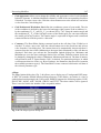
3.2 The Data Editor
The Data Editor is used to assign parameters to the model cells. To load the Data Editor, select
a corresponding item from the Grid, Parameters, Packages or Source menu. For example, if you
want to assign effective porosity to model cells, you will choose Effective Porosity from the
Parameters menu.
The Worksheet shows the plan view of a model layer (Fig. 3.4). An index notation [J, I, K] is used
to describe the location of cells in terms of columns [J], rows [I] and layers [K]. The origin of the
cell indexing system is located at the upper, top, left cell of the model. PMWIN numbers the
layers from the top down, an increment in the K index corresponds to a decrease in elevation. You
can move to another layer by pressing PgDn or PgUp keys or click the Current Layer edit field
in the Toolbar, type the new layer number, and press Enter.
The Data Editor provides two display modes - Local and Global, and two input methods - Cellby-cell and Zone. It also allows you to specify time-dependent model data.
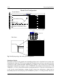
Display Modes
In the Local Display mode, the model grid is displayed parallel to the Worksheet, as shown in Fig.
3.4. In the Global Display mode, the entire worksheet will be displayed (Fig. 3.5). Using the
Environment Options dialog box (see section 3.3.8), you can define the coordinates system and
the size of the worksheet. You can also place the model grid into a proper position. Using the
Maps Options dialog box (see section 3.3.8), you can import DXF site maps.
The Cell-by-Cell Input Method
To activate this method, choose Input Method<Cell-By-Cell from the Options menu. You can
alternatively click the fifth button on the Toolbar until the button becomes
< To assign new value(s) to a cell
1. Click the Assign Value icon
You do not need to click the Assign Value icon, if it is already pressed down.
2. Move the grid cursor to the desired cell by using the arrow keys or by clicking the mouse on
the cell. The value(s) of the current cell will be shown on the Statusbar.
3. Press the right mouse button once
The Data Editor shows a dialog box.
4. In the dialog box, type new value(s) then click OK.
If you double-click a cell, the Data Editor will highlight the cells that have the same value as the
cell. You can hold down the Ctrl key and press the left mouse button to open a Search and
Modify Cell Values dialog box (Fig. 3.6). It allows you to display all cells that have a value
located within the Search Range. According to the user-specified Value and the operation
Options, you can easily modify the cell values. For example, if Add is used, the user-specified
value will be added to the cell value. The Parameter drop-down box contains the available
parameter type(s). You choose a parameter for which the Search and Modify operation will apply.
The Modeling Environment
Processing Modflow
3-5
Fig. 3.4 The Data Editor (Local Display mode)
Fig. 3.5 The Global Display mode of the Data Editor
The Modeling Environment
3-6
Processing Modflow
Fig. 3.6 Search and modify cell values
The Zone Input Method
The Zone Input Method allows you to assign parameters in the form of zones. The zonation
information will also be used by the parameter estimation program PEST. To activate this
method, choose Input Method<Zones from the Options menu. Alternatively, you can click the
fifth button on the Toolbar until the button becomes
< To draw a zone
1. Click the Assign Value icon
You do not need to click the Assign Value icon, if it is already pressed down.
2. Click the mouse cursor on a desired position to anchor one end of a line.
3. Move the mouse to another position then press the left mouse button again.
4. Repeat steps 2 and 3 until the zone is closed or press the right mouse button to abort.
< To assign new value(s) to a zone
1. Click the Assign Value icon
You do not need to click the Assign Value icon, if it is already pressed down.
2. Move the mouse cursor into a zone.
The boundary of the zone will be highlighted. The value(s) of the current zone will be shown
on the Statusbar.
3. Press the right mouse button once.
The Data Editor shows a dialog box.
4. In the dialog box, type new value(s) then click
to transfer the new zone value(s) to cells.
PMWIN always uses the cell data, and if zone data are not transferred, default values within the
cells are used by all other parts of the program, except the parameter optimizing program PEST.
PEST uses the zonation information provided by the zones and the Parameter List. See Chapter 5
for how to use the Parameter List and how to perform model calibrations with PEST.
You can shift a vertex of a zone by pointing the mouse cursor to the vertex node, holding down
the left mouse button while moving the mouse. If you have many zones, some zones can be
crossed or even covered by another. If you move the mouse cursor into a covered zone, the
boundary of the zone will not always be highlighted. In this case, you can move the mouse cursor
into the zone, hold down the Ctrl-key and press the left mouse button once. The Data Editor will
resort the order of the zones and the "lost" zone will be recovered.
The Modeling Environment
Processing Modflow
3-7
Specification of Temporal Data
If your model has more than one stress period, a Temporal Data dialog box appears after you
have clicked the Leave Editor button . This dialog box allows you to manage your temporal
model data. You can edit model data for a particular stress period by selecting a row of the table
and clicking the Edit Data button. If the model data of a stress period are specified, the
corresponding row of the Data column is marked. The Use flag indicates whether the userspecified data should be used for the flow simulation or not. PMWIN uses the data of the previous
stress period, if the Use flag is not marked. You can click on an appropriate box to mark or
unmark the Use flag, if the model data have been specified. Use Copy Data, if you want to copy
model data from a stress period to another.
The following table summarizes the use of the Toolbar buttons of the Data Editor.
Toolbar Button
Action
Leave the Data Editor
Assign Value; Allows you to move the grid cursor and assign values
Zoom In; Allows you to drag a zoom-window over a part of the model
domain.
Zoom Out; Forces the Grid Editor to display the entire worksheet.
Cell-By-Cell Input Method is activated.
Zone Input Method is activated.
Local Display Mode is activated.
Global Display Mode is activated.
Duplication On/Off; If Duplication is turned on, the cell value(s) of the
current cell will be copied to all cells passed by the grid cursor.
Duplication is on, if the small box on the lower-left corner of this icon is
highlighted.
Layer Copy On/Off; If you turn Layer Copy on and then move to an other
layer, the zones and cell values of the current layer will be copied. Layer
Copy is on, if the small box on the lower-left corner of this icon is
highlighted.
The Modeling Environment
3-8
Processing Modflow
3.3 PMWIN Menus
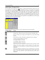
PMWIN contains the menus File, Grid, Parameters, Packages, Source, Estimation, Run, Value,
Options and Help. The Value and Options menus appear only in the Grid Editor and Data Editor.
The following table gives an overview of the menus in PMWIN.
Menu
File
Grid
Parameters
Packages
Source
Estimation
Run
Value
Options
Help
Usage
Create new models; Open existing models; Save plots.
Generate or modify a model grid; Input of the geometry of the grid.
Input of temporal and spatial model parameters, such as transmissivity.
Add specific features of hydrologic system into the groundwater model, such as
wells, recharge or rivers. Define data of an iteration solver and output control.
Specify the source concentration which is associated with a specific features of
hydrologic system, e.g. concentration of water of an injection well.
Specify data for the parameter estimation program PEST.
Call simulation programs, modeling tools and postprocessing utilities.
Manipulate model data; Read or save model data in separate files.
Modify the appearance of the model grid on the screen; Load DXF site maps.
Call the online-Help
PMWIN uses an intelligent menu system to help you control the modeling process. If you have
specified a model data set, the corresponding item of the Grid, Parameters, Packages and Source
menus will be checked. To deactivate a selected item in the Package and Source menu, just
seleted the item again. If you do not know which model data still have to be specified, you can
try to run your model by selecting the corresponding item from the Run menu. PMWIN will tell
you what you should do.
3.3.1 The File Menu
New Model
Select New Model to create a new model. The New Model dialog is a standard Windows dialog
that allows you to choose any available directory or drive on your computer. All filenames valid
under MS-DOS can be used. A PMWIN model file uses the extension MDL. It is a good idea to
save every model in a separate directory, where you can keep the model and its output data. This
will also allow you to run several models simultaneously (multitasking). If a desired directory is
not available, you need to use the File Manager of Windows or other utilities to create the
directory.
Open Model
Use Open Model to load an existing PM model. Models created by using PM3.0x are compatible
to PMWIN. Once a model is opened, PMWIN shows the file name of the model on the Title Bar.
The Modeling Environment
Processing Modflow
3-9
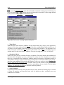
Model Information
Open the Model Information dialog box as shown in Fig. 3.7. This dialog provides brief
information about your model. You can type a simulation title into the dialog. The maximum
length of the simulation title is 132 characters.
Fig. 3.7 The Model Information dialog box
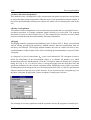
Save Plot As
Use Save Plot As to save the contents of the worksheet in graphics files (Fig. 3.8). Save Plot As
can only be used within the Local Display mode of the Data Editor. Three graphics formats are
available: Drawing Interchange File (DXF), Hewlett-Packard Graphics Language (HP-GL) and
Windows Bitmap (BMP). DXF is a fairly standard format developed by Autodesk for exchanging
data between CAD systems. HP-GL is a two-letter mnemonic graphics language developed by
Hewlett-Packard. These graphics formats can be understood by many graphics or wordprocessing software, and graphics devices. Using the DXF format, you can save and overlay
graphics on the Worksheet, as you can import DXF files by using the Maps Options.
To select a format, click the down-arrow on the Format drop-down box. You can enter the file
name into the File edit field, or click
and select a file from the standard File Open dialog box.
Note that PMWIN uses the same resolution as Windows to save bitmap files. The 24 bits True
Color resolution is not supported by PMWIN. Do not try to save graphics in bitmap files, if you
are using True Color.
Fig. 3.8 The Save Plot As dialog box
The Modeling Environment
3-10
Processing Modflow
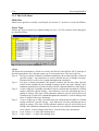
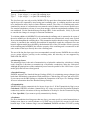
3.3.2 The Grid Menu
Mesh Size
Allows you to generate or modify a model grid. See Section 3.1 for how to use the Grid Editor.
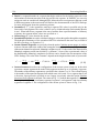
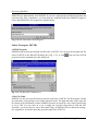
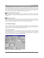
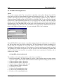
Layer Type
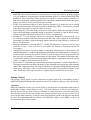
Select Layer Type to open a Layer Options dialog box (Fig. 3.9). The elements of this dialog box
are described below.
Fig. 3.9 The Layer Options dialog box
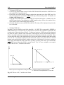
< Type
The numerical formulations, which are used by the Block-Centered-Flow (BCF) package to
describe groundwater flow, depend on the type of each model layer. The layer types are
Type 0 The layer is strictly confined. For transient simulations, the confined storage coefficient
(specific storage × layer thickness) is used to calculate the rate of change in storage.
Transmissivity of each cell is constant throughout the simulation.
Type 1 The layer is strictly unconfined. The option is valid for the first layer only. Specific
yield is used to calculate the rate of change in storage for this layer type. During a flow
simulation, transmissivity of each cell varies with the saturated thickness of the aquifer.
Type 2 A layer of this type is partially convertible between confined and unconfined. Confined
storage coefficient (specific storage × layer thickness) is used to calculated the rate of
change in storage, if the layer is fully saturated, otherwise specific yield will be used.
Transmissivity of each cell is constant throughout the simulation. Vertical leakage from
above is limited if the layer desaturates.
Type 3 A layer of this type is fully convertible between confined and unconfined. Confined
storage coefficient (specific storage × layer thickness) is used to calculate the rate of
change in storage, if the layer is fully saturated, otherwise specific yield will be used.
During a flow simulation, transmissivity of each cell varies with the saturated thickness
of the aquifer. Vertical leakage from above is limited if the layer desaturates.
Type 4 Layer of type 0 + a quasi-3D confining layer.
Type 5 Layer of type 1 + a quasi-3D confining layer
The Modeling Environment
Processing Modflow
Type 6
Type 7
3-11
Layer of type 2 + a quasi-3D confining layer
Layer of type 3 + a quasi-3D confining layer
The last four types are only used by MODPATH for quasi three-dimensional models in which
aquifer layers are separated by intervening semi-confining units. A confining unit does not need
to be simulated as active layers in finite-difference models. The effect of a confining unit can be
simulated by means of a transmission term named vertical leakance between two model layers.
For transient simulations, release of water from storage within the unsimulated confining unit is
not considered. Use the Interbed Storage Package (IBS1; Leake and Prudic, 1988), if you need
to consider the changes in storage for transient simulations.
To calculate pathlines in MODPATH, each unsimulated confining unit is assumed to be a part of
the active model layer directly above it. It is assumed that one-dimensional, steady-state vertical
flow exists throughout the confining layer. This assumption implies that the average vertical linear
velocity is constant in the confining unit and that its magnitude equals the volumetric flow rate
between adjacent model layers divided by the horizontal area of the cell and the effective porosity
of the confining unit. In PMWIN, the effective porosity of the confining unit is assumed to be the
same as that of the layer directly above the confining unit.
The use of the last four layer types is not recommended, not only because PMWIN does not allow
you to assign effective porosity to the confining units, but also they are not supported by
PMPATH and MT3D.
< Anisotropy factor
The anisotropy factor is the ratio of transmissivity or hydraulic conductivity (whichever is being
used) along the I-direction to transmissivity or hydraulic conductivity along the J-direction.
Although the principal axes of the conductivity tensor must be parallel to the I and J-axes of your
model grid, this has been often ignored.
< Interbed Storage
PMWIN supportes the Interbed-Storage Package (IBS1) for calculating storage changes from
both elastic and inelastic compaction of each model layer. Click the flag of a layer and select YES,
if you want to use the IBS1 package to calculate the compaction of the layer. See Packages Menu
for more information about the Interbed Storage Package.
< Transmissivity
MODFLOW requires transmissivity for layers of type 0 or 2. If the Transmissivity flag is set to
Calculated, PMWIN calculates transmissivity by using user-specified horizontal hydraulic
conductivity and the elevations of the top and bottom of each layer. Set the Transmissivity flag
to User Specified, if you want to specify transmissivity directly.
< Leakance
For flow simulations involving more than one layer, you must specify a vertical transmission or
leakage term, know as vertical leakance or VCONT array, for each cell, except for cells in the
bottom layer. If the Leakance flag is set to Calculated, PMWIN calculates VCONT by using
The Modeling Environment
3-12
Processing Modflow
user-specified vertical hydraulic conductivity and the elevations of the top and bottom of each
layer. Set the Leakance flag to User Specified, if you want to specify VCONT (vertical leakance)
directly. See Parameters menu for more information about how to calculate VCONT.
< Storage Coefficient
For transient flow simulations, MODFLOW requires dimensionless storage terms specified for
each model layer. For a confined layer, these storage terms are given by the confined storage
coefficient (=specific storage [L-1] × layer thickness [L]). If the Storage Coefficient flag is
Calculated, PMWIN uses user-specified specific storage and the elevations of the top and bottom
of each layer to calculate the confined storage coefficient. Set the Storage Coefficient flag to User
Specified, if you want to specify the confined storage coefficient directly. For an unconfined
layer, the storage values are equal to specific yield [-]. The setting of the Storage Coefficient flag
has no influence on the input of specific yield.
Boundary Condition
An IBOUND array is required by flow models. The IBOUND array contains a code for each
model cell which indicates whether (1) the hydraulic head is computed (active variable-head cell
or active cell), (2) the hydraulic head is kept fixed at a given value (constant-head cell or timevarying specified-head cell), or (3) no flow takes place within the cell (inactive cell). It is
suggested to use 1 for an active cell, -1 for a constant-head cell, and 0 for an inactive cell. For
constant-head cells, the initial hydraulic head remains the same throughout the simulation. The
initial hydraulic head is specified by choosing Starting Values<Hydraulic Heads from the
Parameters menu. A constant head boundary exists whenever the aquifer is in direct hydraulic
contact with a river, a lake or a reservoir in which the water level is known. It is important to
know that a specified head boundary provides inexhaustible supply of water. The groundwater
system may get as much water as it needs from the constant head boundary. In some situations,
this may be unrealistic. You should thus be careful in setting constant head boundaries. Consider
to use the General-Head Boundary (GHB1) or the Time-Variant Specified-Head (CHD1)
packages, if the head at the prescribed head boundary varies with the time.
An ICBUND array is required by transport models. The ICBUND array contains a code for each
model cell which indicates whether (1) the concentration varies with time (active concentration
cell), (2) the concentration is constant (constant-concentration cell), or (3) the cell is an inactive
concentration cell. It is suggested to use 1 for an active concentration cell, -1 for a constantconcentration cell, and 0 for an inactive concentration cell. In MT3D, no-flow or dry cells are
automatically converted into inactive concentration cells. Active variable-head cells can be treated
as inactive concentration cells to minimize the area needed for transport simulation, as long as the
solute transport is insignificant near those cells. For constant-concentration cells, the starting
concentration remains the same at the cell throughout the simulation. A constant-head cell may
or may not be a constant-concentration cell. The starting concentration is specified by choosing
Starting Values<Concentration from the Parameters menu.
Top of Layers (TOP)
MODFLOW reads the top elevation only for layers of type 2 or 3. Top of Layers is required, if
you want to use PMPATH, MT3D and MODPATH, or if you let PMWIN calculate
The Modeling Environment
Processing Modflow
3-13
transmissivity, vertical leakance or confined storage coefficient (see Layer Type above).
Bottom of Layers (BOT)
MODFLOW reads the bottom elevation only for layers of type 1 or 3. Bottom of Layers is
required, if you want to use PMPATH, MT3D and MODPATH, or if you let PMWIN calculate
transmissivity, vertical leakance or confined storage coefficient (see Layer Type above).
3.3.3 The Parameters Menu
Time
You specify temporal parameters in the Time Parameters dialog box as shown in Fig. 3-10. To
activate a stress period, click the Active flag and set it to YES. The temporal parameters include
the time unit, the length of stress periods and the numbers of stress periods, time steps and
transport steps. In MODFLOW, the simulation time is divided into stress periods, which are, in
turn, divided into time steps. In the MT3D model, each time step is further divided into smaller
time increments, called transport steps.
Fig. 3.10 The Time Parameters dialog box
Each time you select a time unit from the Simulation Time Unit group, PMWIN will update the
Period Length in the table, if Auto Update Period Length is checked. PMWIN allows you to
perform steady state or transient flow simulations by selecting a corresponding option from the
Simulation Flow Type group. You can run a steady state simulation over several stress periods.
In this case, a steady state solution is calculated for each stress period.
For each stress period, you have the option of changing parameters associated with head-dependent
boundary conditions in the River, Stream, Drain, Evapotranspiration, General-Head Boundary and
Time-Variant Specified-Head Boundary Packages, as well as the recharge rates in the Recharge
Package and pumping rates in the Well Package. For transport simulations, you can change source
The Modeling Environment
3-14
Processing Modflow
concentration associated with Well, River, Stream, Recharge, Evapotranspiration and General-Head
Boundary Packages as well as Constant-Head cells.
Using the buttons Save and Load, you can save or load the contents of the table in or from a time
parameter file. The format of the time parameter file is given in Appendix 2.
MODFLOW allows the time step to increase as the simulation progesses. It uses the following
formulae to increase the lengths of time steps as a geometric progression.
Delt(1) '
PERLEN @ (1 & TSMULT)
1 & TSMULT NSTP
Delt(m%1) ' TSMULT @ Delt(m)
(3.1)
(3.2)
where PERLEN is the length of a stress period, TSMULT is the time step multiplier, NSTP is
the number of time steps and Delt(m) is the length of time step m in a stress period.
The length of stress periods is not relevant to steady state flow simulations. However, if you want
to perform contaminant transport simulation with MT3D at a later time, you must specify the actual
time length in the table. Because the explicit transport solution (MT3D, version 1.85) has certain
stability criteria associated with it, the length of a time step used for a head solution may be too
large for a transport solution. Each time step is, therefore, divided into smaller transport steps.
You can specify the length of transport steps in the table of the Time Parameters dialog box. The
length of transport steps will be determined by an automatic stepsize control procedure in MT3D,
if the length of transport steps is 0 (zero).
Recycle
Recycle provides a way to create graphics from simulation results. You can freely modify the Recycle
data in the Data Editor, because neither simulation programs nor any parts of PMWIN will use
the Recycle data. See Chapter 2 for how to produce output graphics.
Starting Values
MODFLOW requires initial hydraulic heads at the beginning of a flow simulation. Initial hydraulic
heads at constant-head cells will be kept constant during the flow simulation. The initial hydraulic
heads in constant-head cells must be higher than the elevation of the bottom of these cells, because
MODFLOW does not convert dry constant-head cells to inactive cells. If any constant-head cell
is dry, MODFLOW will stop the flow simulation and write a message "CONSTANT-HEAD CELL
WENT DRY" into a run record file (see Table 2.1).
MODFLOW also requires initial heads in a steady state simulation. In that case the intial values
are starting values for the iterative equation solvers. Note that the heads at the prescribed head
cells must be the actual model values while all other initial heads can be set arbitrarily, provided
they are higher than the bottom elevation of the cells.
The Modeling Environment
Processing Modflow
3-15
MT3D requires initial concentration at the beginning of a transport simulation. Initial concentration
at constant-concentration cells will be kept constant during the simulation. Constant-concentration
cells can be used to simulate contaminated areas with constant concentration.
Horizontal Hydraulic Conductivity and Transmissivity
Horizontal hydraulic conductivity is the hydraulic conductivity along model rows. It is multiplied
by an anisotropy factor specified in the Layer Options dialog to obtain the hydraulic conductivity
along model columns. Horizontal hydraulic conductivity is required for layers of type 1 or 3.
Transmissivity is required for layers of type 0 and 2.
PMWIN uses the horizontal hydraulic conductivity and layer thickness to calculate transmissivity,
if the corresponding Transmissivity flag in the Layer Options dialog is Calculated. You can specify
transmissivity of a layer directly by setting the corresponding Transmissivity flag to User-specified
and choosing Transmissivity from the Parameters menu. See section 3.2.2 for more information
about the Layer Options dialog.
Vertical Hydraulic Conductivity and Vertical Leakance
For flow simulations involving more than one model layer, MODFLOW requires the input of
the vertical transmission or leakage term, known as vertical leakance (VCONT), between two model
layers. PMWIN uses the vertical hydraulic conductivities and thicknesses of layers to calculate
VCONT, if the corresponding Leakance flag in the Layer Options dialog is Calculated.
VCONT '
2
)v k
(K z)i,j,k
%
)vk%1
(3.3)
(Kz)i,j,k%1
where (Kz)i,j,k and (Kz)i,j,k%1 are the vertical hydraulic conductivities of layers k and k+1, respectively.
Refer to Fig. 3.11a for definition of )vk and )vk%1 . Equation 3.3 is used when each model layer
represents a different hydrostratigraphic unit or when two or more model layers represent a single
hydrostratigraphic unit.
Fig. 3.11 Grid configurations used for the calculation of VCONT
The Modeling Environment
3-16
Processing Modflow
For quasi three-dimensional models that contain unsimulated semiconfining units, VCONT must
be specified by the user directly. In this case, VCONT can be calculated by using the following equation.
VCONT '
)zu
(K z)u
%
2
2)zc
(Kz)c
%
)zL
(3.4)
(Kz)L
where (Kz)u , (Kz)c and (Kz)L are the vertical hydraulic conditivities of the upper layer, semiconfining
unit and lower layer, respectively. Refer to Fig. 3.11b for definition of )zu , )zc and )zL . You
can specify VCONT by setting the corresponding Leakance flag in the Layer Options dialog box
to User-specified and choosing Vertical Leakance from the Parameters menu. In the Data Editor,
VCONT between layer i and layer i+1 is given as the data of layer i. A VCONT array is not required
for the bottom layer because MODFLOW assumes that the botton layer is underlain by impermeable
material and VCONT is zero.
Specific Storage, Storage Coefficient and Specific Yield
For transient flow simulations, MODFLOW requires dimensionless storage terms specified for
each layer of the model. For a steady state simulation, these menu items are not used and dimmed.
In a confined layer, the storage term is given by storativity or confined storage coefficient (=specific
storage [L-1] × layer thickness [L]). The specific storage or specific storativity is defined as the
volume of water that a unit column of aquifer releases from storage under a unit decline in hydraulic
head. The confined storage coefficient is required by layers of type 0, 2 and 3. PMWIN uses specific
storage and the layer thickness to calculate the confined storage coefficient, if the corresponding
Storage Coefficient flag in the Layer Options dialog is Calculated. By setting the Storage Coefficient
flag to User Specified and choosing Storage Coefficient from the Parameters menu, you can specify
the confined storage coefficient directly.
In an unconfined layer, the storage term is given by specific yield or unconfined storativity. Specific
yield is defined as the volume of water that an unconfined aquifer releases from storage per unit
surface area of aquifer per unit decline in the water table. Specific yield is required for layers of
type 1, 2 and 3.
Refer to Bear (1972) or Freeze and Cherry (1979) for more information about the storage terms
and their definitions.
Effective Porosity
Effective porosity is used by the programs PMPATH, MODPATH and MT3D to calculate the
average velocity of the flow through the porous medium.
The Modeling Environment
Processing Modflow
3-17
3.3.4 The Packages Menu
Well (WEL1)
In Modflow, an injection or a pumping well is represented by a model cell. The injection or pumping
rates are specified by using the Data Editor. Negative cell values are used to indicate pumping wells,
while positive cell values indicate injection wells.
The injection or pumping rate of a well is constant during a given stress period and is independent
of both the cell area and the head in the cell. It is implicitly assumed by MODFLOW that a well
penetrates the full thickness of the cell. MODFLOW can simulate wells that penetrates more than
one model layer. In this case, the injection or pumping rate for each layer has to be specified. The
total injection or pumping rate for a multilayer well is equal to the sum of those from the individual
layers. The injection or pumping rate for each layer ( Qk ) can be approximately calculated by dividing
the total rate ( Qtotal ) in proportion to the layer transmissivities (McDonald and Harbaugh, 1988):
Q k ' Qtotal @
Tk
ET
(3.5)
where Tk is the transmissivity of layer k and ET is the sum of the transmissivities of all layers
penetrated by the multilayer well.
An other possibility to simulate multi-layer wells is to set a very large vertical hydraulic conductivity
or vertical leakance, e.g., 1 [m/s] or 0.1 [1/s], to all cells of the well. The injection or pumping rate
for each penetrated layer can be equal to the total rate ( Qtotal ) divided by the number of the penetrated
layers. In this case, the exact rates for each penetrated layer will be calculated by MODFLOW
implicitly. The exact flow rates can be obtained by using the Water Budget Calculator. See Chapter
2 for how to calculate subregional water budgets.
Drain (DRN1)
Drains are defined by using the Data Editor to assign two values to model cells (Fig. 3.12):
- Drain hydraulic conductance ( Cd ) [L2T-1]
- Median elevation of the Drain ( d ) [L]
The values Cd and d are shown on the Statusbar. These values are constant during a given stress
period. For transient flow simulations involving several stress periods, these values can be different
from period to period.
When the hydraulic head (h) in a drain-cell is greater than the drain elevation, water flows into
the drain and is removed from the groundwater model. Discharge to the drain is zero when the
hydraulic head is lower than or equal to the median drain elevation. Recharge from the drain is
always zero, regardless of the hydraulic head in the aquifer. Discharge rate to the drain ( Qd ) is
calculated by
Q d ' Cd @ (h & d)
(3.6)
The Modeling Environment
3-18
Processing Modflow
The value Cd of a drain-cell is often given by
Cd ' K @ L
(3.7)
where L is the length of the drain within a cell. The value K is a equivalent hydraulic conductivity
describing all of the head loss between the drain and the aquifer. It depends on the material and
characteristics of the drain itself and the immediate environment. The value Cd is usually unknown
and must be adjusted during a model calibration.
Fig. 3.12 The Drain (DRN1) dialog box
General-Head Boundary (GHB1)
The General-Head Boundary Package (GHB1) is used to simulate head-dependent flow boundaries
(Cauchy boundary conditions). Similar to the Drain Package, a General-Head Boundary cell (GHB-cell)
is defined by two cell values:
- GHB hydraulic conductance Cb [L2T-1]
- Hydraulic head at the boundary hb [L]
The values Cb and hb of a GHB-cell are shown on the Statusbar. Flow through the general-head
boundary Qb [L3T-1] is calculated by
Q b ' Cb (h b & h)
(3.8)
where h is the hydraulic head in the aquifer. A GHB-cell is equivalent to a constant head cell, if
a large Cb is used. The values Cb and hb are constant during a given stress period. For transient flow
simulations involving several stress periods, these values can be different from period to period.
This allows you to change the head at "constant-head" boundaries as the transient simulation
progresses.
River (RIV1)
The River Package is used to simulate the flow between an aquifer and a surface-water feature,
such as rivers, lakes or reservoirs. Rivers are defined by using the Data Editor to assign the following
three values to the model cells:
- Hydraulic conductance of the riverbed (CRIV) [L2T-1]
- Head in the river (HRIV) [L], and
- Elevation of the bottom of the riverbed (RBOT) [L].
The Modeling Environment
Processing Modflow
3-19
The values CRIV, HRIV and RBOTof a river-cell are shown from left to right on the Statusbar.
For transient flow simulations involving several stress periods, these values can be different from
period to period. If the hydraulic head (h) in a river-cell is greater than RBOT, the rate of leakage
(QRIV) from the river to the aquifer is calculated by:
QRIV ' CRIV@(HRIV & h)
h>RBOT
(3.9)
For the case that h is greater than HRIV, QRIV is negative. It means that water flows from the
aquifer into the river and is removed from the groundwater model. When h has fallen below the
bottom of the riverbed, the rate of leakage through the riverbed is given by:
QRIV ' CRIV@(HRIV & RBOT)
h#RBOT
(3.10)
The value CRIV of a river-cell is often given by
CRIV '
K@L@W
M
(3.11)
where the value K is the hydraulic conductivity of the riverbed material, L is the length of the river
within a cell, W is the width of the river and M is the thickness of the riverbed. If CRIV is unknown,
it must be adjusted during a model calibration.
Streamflow-Routing (STR1)
The Streamflow-Routing Package STR1 (Prudic, 1989) is designed to account for the amount
of flow in streams and to simulate the interaction between surface streams and groundwater. Streams
are divided into segments and reaches. Each reach corresponds to individual cells in the finite-difference
grid. A segment consists of a group of reaches connected in downstream order. Streamflow is
accounted for by specifying flow for the first reach in each segment, and then computing streamflow
to adjacent downstream reaches in each segment as equal to inflow in the upstream reach plus or
minus leakage from or to the aquifer in the upstream reach. The accounting scheme used in STR1
assumes that streamflow entering the modeled layer is instantly available to downstream reaches.
This assumption is generally reasonable because of the relatively slow rates of groundwater flow.
Streamflow into a segment that is formed from tributary streams is computed by adding the outflows
from the last reach in each of the specified tributary segments. If a segment is a diversion, then
the specified flow into the first reach of the segment is subtracted from flow in the main stream.
However, if the specified flow of the diversion is greater than the flow out of the segment from
which flow is to be diverted, then no flow is diverted from that segment.
In the Data Editor, you can press the right mouse button and specify the following required cell
values in the Streamflow-Routine Package (STR1) dialog box. The specified cell values will be
shown on the Statusbar.
< Segment is a number assigned to a group of reaches. Segments must be numbered in downstream
order. The maximum number allowed in PMWIN is 25.
The Modeling Environment
3-20
Processing Modflow
< Reach is a sequential number in a segment that begins with one for the farthest upstream reach
and continues in downstream order to the last reach in the segment. In PMWIN, you can only
assign one reach to a model cell, although STR1 allows the user to assign more than one reach
in different segments to the same model cell. Refer to the documentation of the STR1 Package
for more information about the numbering scheme.
< Streamflow [L3T-1] is the streamflow entering a segment. This value is specified only for the
first reach in each segment. The value is either a zero or a blank when the reach number (Reach)
is not 1. When inflow into a segment is the sum of outflow from a specified number of tributary
segments, the segment inflow values are specified as -1.
< Stream Stage [L] is the head in the stream.
< Streambed Properties are used to calculate leakage to or from the aquifer through the streambed.
The hydraulic conductance of the streambed CSTR is calculated in the same way as CRIV of
the River Package, see Equation 3.11.
< Stream Channel Properties are used only when the option Calculate stream stages in reaches
is chosen. Stream width is the width of the rectangular stream channel. Stream Slope is the slope
of the stream channel in each reach. Manning's roughness coeff./C is the result of the dimensionless
Manning's roughness coefficient divided by a constant C. Some of the experimental values of
the dimensionless Manning's roughness coefficient can be found in the documentation of the
STR1 Package. The value of the constant C depends on the length and time units of your model.
C ' 1
m 1/3
ft 1/3
ft 1/3
m 1/3
' 1.486
' 1.7198@10&5
' 1.1574@10&5
s
s
d
d
(3.12)
< Stream Structure describes the configuration of the stream system. Each row in the table
represents a stream segment in the model. Each segment can have up to 10 tributary segments.
The number of the tributary segments are specified in the columns 1 to 10. The column Iupseg
is the number of the upstream segment from which water is diverted. For a segment that is not
a diversion, Iupseg must be specified as zero. Iupseg is used only when the option Simulate
diversions from segments is checked. The values in Fig. 3.13 indicate that segment 2 is diverted
from segment 1, segment 1 is a tributary segment of segment 3, and segments 2 and 4 are tributary
segments of segment 5. The configuration of the stream system is shown in Fig. 3.14.
The Modeling Environment
Processing Modflow
3-21
Fig. 3.13 The Streamflow-Routine Package (STR1) dialog box
Fig. 3.14 The configuration of the stream system specified in the table of figure 3.13
Similar to the River Package, leakage (Q1) to or from the aquifer through the streambed is computed
by Darcy's Law as follows:
Q1 ' CSTR@(H s & h)
Q1 ' CSTR@(H s & SBOT )
h>SBOT
h#SBOT
(3.13)
where CSTR is the hydraulic conductance of the streambed, Hs is the head in the stream, h is the
head in the model cell beneath the streambed and SBOT is the elevation of the bottom of the stream.
The Modeling Environment
3-22
Processing Modflow
If the option Calculate stream stages in reaches is checked, the depth (d) in each reach is calculated
from Manning's equation under the assumption of a rectangular stream channel:
d '
Q@ n
3/5
C@ w@ S 1/2
(3.14)
where Q [L3T-1] is the stream discharge calculated by STR1, n [ - ] is Manning's roughness coefficient,
w [L] is the width of the channel, S [LL-1] is the slope of the stream channel and C is a constant
(see equation 3.12).
Recharge (RCH1)
The Recharge Package is designed to simulate areally distributed recharge to the groundwater system.
Recharge is defined by assigning the following data to model cells in the Recharge (RCH1) dialog
box (Fig. 3.15):
- Recharge Flux IR [LT-1]
- Layer Indicator IRCH [-]
The specified values IR and IRCH are shown on the Statusbar of the Data Editor. Note that although
IR and IRCH are specified for each vertical column of cells, you are allowed to move to other layers
within the Data Editor and examine the grid configuration in each layer.
Fig. 3.15 The Recharge (RCH1) dialog box
MODFLOW uses IR to calculate the recharge flow rate (QR [L3T-1]) applied to the model cell:
Q R ' IR @ DELR @ DELC
(3.15)
where DELR @ DELC is the map area of a model cell. The recharge rate QR is applied to a single
cell within a vertical column of cells. There is no need to allow for recharge to occur simultaneously
at multiple depths in the same vertical column because natural recharge enters the groundwater
system at the water table. In the simplest situation, the water table is located in the top layer of
the model. The top layer is designated as unconfined and an array of Recharge Flux IR is specified
The Modeling Environment
Processing Modflow
3-23
for that layer. Problems may arise, when the water table cuts across layers. To solve this kind of
problems, the RCH1 Package provides three options for specifying the cell in each vertical column
of cells that receives the recharge:
1. Recharge is only applied to the top grid layer
2. Vertical distribution of recharge is specified in the Layer Indicator Array. IRCH defines the layer
where recharge is applied.
3. Recharge is applied to the highest active cell in each vertical column. The user does not have
to predetermine the layer to which recharge should be applied. The appropriate layer is
automatically selected by the RCH1 Package. If the highest active cell is a constant-head cell
recharge will be intercepted and cannot go deeper.
Evapotranspiration (EVT1)
The Evapotranspiration Package simulates the effects of plant transpiration and direct evaporation
in removing water from the saturated groundwater regime. The EVT1 Package requires the user
to assign the following data for each EVT-cell in the Evapotranspiration (EVT1) dialog box (Fig. 3.16).
-
Maximum ET Rate RETM [LT-1],
Elevation of the ET Surface hs [L],
ET Extinction Depth d [L], and
Layer Indicator IET [-]
The specified values will be shown on the Statusbar. Note that although the values are specified
for each vertical column of cells, you are allowed to move to other layers within the Data Editor
and examine the grid configuration in each layer.
Fig. 3.16 The Evapotranspiration (EVT1) dialog box
The EVT1 Package is based on the following assumptions:
1. When water table is at or above the elevation of the ET surface hs , evapotranspiration loss
from the water table is at the maximum ET Rate RETM;
2. No evapotranspiration occurs when the depth of the water table below the elevation of the ET
surface exceeds the ET extinction depth d; and
3. In between these two extremes evapotranspiration varies linearly with the water table elevation.
The Modeling Environment
3-24
Processing Modflow
These assumptions can be expressed in equation form as:
RET ' RETM
RET ' 0
RET ' RETM @
h>h s
h<h s&d
d & (hs & d )
d
(3.16)
(h s&d) # h# h s
where RET [L3L-2T-1] is the evapotranspiration rate per unit of surface area of water table. The
evapotranspiration flow rate (QET [L3T-1]) drawn from a model cell is
Q ET ' RET @ DELR @ DELC
(3.17)
where DELR @ DELC is the map area of a model cell. QET is drawn from only one cell in the vertical
column beneath the map area DELR @ DELC . The EVT1 Package provides two options for specifying
the cell in each vertical column of cells where evapotranspiration is drawn from:
1. Evapotranspiration is always drawn from the top layer of the model.
2. Vertical distribution of evapotranspiration is specified in the Layer Indicator Array. IET defines
the layer where evapotranspiration is drawn from.
In either case the QET has no influence on the simulation if the designated cell is either a no-flow
(inactive) cell or a constant head cell. You can select an option in the Evapotranspiration (EVT1)
dialog box. The layer indicator array is needed only when the second option is used.
Horizontal-Flow Barrier (HFB1)
The Horizontal-Flow Barrier Package (Hsieh and Freckleton, 1993) simulates thin low-permeability
geologic features, such as vertical faults or slurry walls, that impede the horizontal flow of groundwater.
These geologic features are approximated as a series of horizontal-flow barriers conceptually situated
on the boundaries between pairs of adjacent cells in the finite-difference grid.
A horizontal-flow barrier is defined by assigning the following values to a model cell in the HorizontalFlow Barrier (HFB1) dialog box (Fig. 3.17):
- Barrier Direction [-]; and
- (Hydraulic Conductivity/Thickness) of the barrier TDW [T-1]
The barrier direction indicates the cell face where the barrier is located. To erase an existing barrier,
use zero for the barrier direction. The second value TDW gives the hydraulic characteristic of the
barrier. In the HFB1 Package, barrier thickness is included implicitly in TDW. If the layer type is
1 or 3, TDW will be used by the HFB1 Package directly. If a layer is confined (type 0 or 2), however,
PMWIN assigns the product of TDW and the layer thickness to the HFB1 Package. In this case,
you have to specify the elevations of the top and bottom of these layers, although these elevations
are not always required for simulating confined layers.
For the numerical implementation of the Horizontal-Flow Barrier Package refer to Hsieh and Freckleton
(1993).
The Modeling Environment
Processing Modflow
3-25
Fig. 3.17 The Horizontal-Flow Barrier (HFB1) dialog box
Interbed Storage (IBS1)
For steady state flow simulations, the menu Interbed Storage (IBS1) is not used and dimmed. The
Interbed Storage Package (Leake and Prudic, 1991) simulates elastic and inelastic compaction of
compressible fine-grained beds due to groundwater extraction. The term "interbed" is used to denote
a poorly permeable bed within a relatively permeable aquifer.
To incorporate the calculation of interbed storage of a layer, set the Interbed Storage flag to YES
(see Layer Options dialog in section 3.3.2). The data required by the IBS1 Package are specified
by using the Data Editor in the Interbed Storage dialog box (Fig. 3.18):
- Preconsolidation Head or preconsolidation stress Hc [L] in terms of head in the aquifer.
Preconsolidation head is the previous minimum head value in the aquifer. For any model cells
in which the specified preconsolidation head is greater than the corresponding value of initial
head, the value of the preconsolidation head will be set to that of the initial head;
- Elastic Storage Factor Sfe [-] for interbeds present in the model layer;
- Inelastic Storage Factor Sfv [-] for interbeds present in the model layer;
- Starting Compaction [L]. Compaction values computed by the IBS1 Package are added to Starting
Compaction so that stored values of compaction and land subsidence may include previous
components. Starting Compaction does not affect calculations of storage changes or resulting
compaction.
Fig. 3.18 The Interbed Storage (IBS1) dialog box
The Modeling Environment
3-26
Processing Modflow
For a confined aquifer, elastic compaction or expansion of sediments is proportional or nearly
proportional to change in hydraulic head in the aquifer. The IBS1 Package uses the following equation
to calculate the change in thickness:
)b ' &)h @ S ske@ b0 ' &)h@ Sfe
(3.18)
where )b [L] is change in thickness, positive for compaction and negative for expansion; ) h[L]
is change in hydraulic head, positive for increase;Sske [L-1] is the skeletal component of elastic specific
storage; b0 is the thickness of the interbed; and Sfe is the user-specified elastic storage factor. When
compressible fine-grained sediments are stressed beyond a previous maximum stress (preconsolidation
stress), compaction is permanent (inelastic). In analogy to equation 3.18, the IBS1 package uses
the following equation to calculate the approximate inelastic compaction )b* [L]:
)b ( ' &)h@ S skv@ b0 ' &)h@ Sfv
(3.19)
where Sskv [L-1] is the skeletal component of inelastic specific storage and Sfv is the user-specified
inelastic storage factor.
For an unconfined aquifer, elastic compaction or expansion of sediments can be expressed as
)b ' &)h @ (1& n% n w ) @ S ske@ b0 ' &)h@ S fe
(3.20)
where n [-] is porosity and nw [-] is moisture content above water table as a fraction of total volumn
of porous medium. Similarly, inelastic compaction or expansion of sediments can be expressed
as
)b ' &)h @ (1& n% n w ) @ S skv@ b0 ' &)h@ S fv
(3.21)
For an aquifer with n interbeds with specific-storage values Ss1, Ss2,..., Ssn and with thicknesses
b1, b2, ..., bn , a single equivalent storage factor Ssytem [-] is given by Jorgenson (1980):
S system' Ss1b1% S s2b2 %...% S snb n
(3.22)
For the numerical implementation of the Interbed Storage Package refer to Leake and Prudic (1991).
Time-Variant Specified-Head (CHD1)
For transient simulations, the Time-Variant Specified-Head Package (Leake and Prudic, 1991)
allows constant-head cells to take on different head values for each time step. You use the Time-Variant
Specified-Head (CHD1) dialog box to specify the data required by the CHD1 Package (Fig. 3.19):
- Flag [-]. A non-zero value indicates that a cell is specified as a time-variant specified-head boundary.
- Start Head hs [L]. This value is the head in the cell at the start of the stress period.
- End Head he [L]. This value is the head that will be assigned to the cell for the last time step
in the stress period.
The Modeling Environment
Processing Modflow
3-27
The CHD1 Package does not alter the way constant-head boundaries are formulated in the finitedifference equations of MODFLOW. CHD1 sets the element in the IBOUND array to a negative
value for all cells where a time-variant specified-head boundary is selected (Flag…0). The specified
heads are constant during a time step. The CHD1 Package linearly interpolates boundary heads h
for each time-variant specified-head boundary cell by using the equation:
h ' h s % (h e & h s) @
PERTIM
PERLEN
(3.23)
where PERTIM is the staring time of a time step in a stress period and PERLEN is the length of
the whole stress period.
Fig. 3.19 The Time-Variant Specified-Head (CHD1) dialog box
Wetting Capability (BCF2)
The wetting capability of the Block-Centered Flow 2 Package (BCF2; McDonald et al. 1991) allows
the simulation of a rising water table into unsaturated (dry) model layers. The BCF2 Package is
identical to the BCF1 Package of the "original" MODFLOW (McDonald and Harbaugh, 1988)
except for the wetting and drying of cells. In BCF1, a cell falls dry when the head is below the bottom
elevation of the cell. When a cell falls dry, IBOUND is set to 0 (which indicates no flow or inactive
cell), all conductances to the dry cell are set to zero. The cell cannot be wetted again. In BCF2,
a dry cell or an inactive cell can become wet if the head from the previous iteration in a neighboring
cell is greater than or equal to the turn-on threshold. The turn-on threshold is
TURNON ' BOT % |THRESH|
(3.24)
where BOT is the elevation of the bottom of the cell and THRESH is a user-specified constant called
the wetting threshold. A non-zero value THRESH is specified for each cell that can be wetted.
If THRESH<0, only the cell below a dry cell can cause the cell to become wet. If THRESH>0,
the cell below a dry cell and the four horizontally adjacent cells can cause the cell to become wet.
If THRESH is zero, the dry cell or the inactive cell cannot be wetted.
The Modeling Environment
3-28
Processing Modflow
Only variable-head cells either immediately below or horizontally adjacent to a dry cell can cause
the cell to become wet. A neighboring cell cannot become wet as a result of a cell that has become
wet in the same iteration. When a cell is wetted, IBOUND for the cell is set to 1 (which indicates
a variable-head cell), vertical conductances are set to their original values, and the hydraulic head
h at the cell is set equal to one of the following
h ' BOT % WETFCT(hn & BOT )
(3.25)
h ' BOT % WETFCT@ |THRESH|
(3.26)
where hn is the head at the neighboring cell that causes the dry cell to wet, and WETFCT is a userspecified constant called the wetting factor. The user can select between equation 3.25 and 3.26
in the Wetting Capability (BCF2) dialog box (Fig. 3.20). This dialog box appears when you select
Wetting Capability (BCF2) from the Packages menu. The dialog also allows you to specify the
iteration interval for attempting to wet cells IWETIT. Wetting is attempted every IWETIT iterations.
If using the PCG2 solver (Hill, 1990), this applies to outer iterations, not inner iterations. The reason
of adjusting IWETIT is that the wetting of cells sometimes produces erroneous head changes in
neighboring cells during the succeeding iteration, which would cause erroneous conversions of
those cells. These erroneous conversions can be prevented by waiting a few iterations until heads
have had a chance to adjust before testing for additional conversions. When setting IWETIT greater
than one, there is some risk that cells may be prevented from correctly converting from dry to wet.
If the solution for a time step is obtained in less than IWETIT iterations, then there will be no check
during that time step to see if cells should be converted from dry to wet. The potential for this problem
to occur is greater in transient simulations, which frequently require only a few iterations for a time
step.
The method of wetting and drying cells used in the BCF2 Package can cause problems with the
convergence of the iterative solvers used in MODFLOW. Convergence problems can occur in
MODFLOW even without the wetting capability but problems are more likely to occur when the
wetting capability is used. Symptoms of a problem are slow convergence or divergence combined
with the frequent wetting and drying of the same cells. It is normal for the same cell to convert
between wet and dry several times during the convergence process. but frequent conversions are
an indication of problems. The user can detect this situation by examining the model run record
file OUTPUT.DAT; a message is printed each time a cell converts. Refer to the documentation
of the BCF2 Package for how to solve problems with convergence. As a matter of fact, situations
exist where the real solution is oscillating such as in the case of a well causing a drawdown which
makes the well cell fall dry. This in turn switches off the well and leads to a rise of the water table
and wetting of the well cell etc.
The Modeling Environment
Processing Modflow
3-29
Fig. 3.20 The Wetting Capability (BCF2) dialog box
Advection (MTADV1)
The MT3D model provides four solution schemes for the advection term. The user can select a
solution scheme in the Advection Package (MTADV1) dialog box (Fig. 3.21).
The method of characteristics (MOC) scheme was implemented in the U.S. Geological Survey
two-dimensional transport model (Konikow and Bredehoeft, 1978), and has been widely used.
Using the MOC scheme, a set of moving particles is distributed in the flow field at the beginning
of the simulation. A concentration and a position in the Cartesian coordinate system are associated
with each of these particles. Particles are tracked forward through the flow field using a small time
increment. At the end of each time increment, the average concentration at a cell due to advection
alone is evaluated from the concentrations of particles which happen to be located within the cell.
One of the most desirable features of the MOC technique is that it is virtually free of numerical
dispersion, which creates serious difficulty in many numerical schemes. The major drawback of
the MOC scheme is that it can be slow and requires a large amount of computer memory when
a large amount of particles is required. In the MT3D model, instead of placing a uniform number
of particles in every finite-difference cell, a dynamic approach is used to control the distribution
of moving particles. The number of particles placed at each cell is normally set either at a high level
or at a low level, according to the so-called "relative cell concentration gradient", or DCCELL,
defined as:
DCCELLi,j,k '
CMAXi,j,k & CMINi,j,k
CMAX & CMIN
(3.27)
where CMAXi, j, k is the maximum concentration in the immediate vicinity of the cell (i, j, k); CMINi, j, k
is the minimum concentration in the immediate vicinity of the cell (i, j, k); CMAX is the maximum
concentration in the entire grid; and CMIN is the minimum concentration in the entire grid. With
the dynamic approach, the user defines a criterion DCEPS; the higher number of particles, NPH,
is placed in cells where the relative concentration gradient is greater than DCEPS, and the lower
number of particles, NPL, in cells where the relative concentration gradient is less than DCEPS.
In many practical problems involving solute transport modeling, the contaminant plumes may occupy
only a small fraction of the finite-difference grid and the concentrations may be changing rapidly
only at sharp fronts. In these cases, the number of total particles used is much smaller than required
The Modeling Environment
3-30
Processing Modflow
in the uniform particle distribution approach, thereby the efficiency of the method-of characteristics
model can be increased with little loss in accuracy.
Fig. 3.21 The Advection Package (MTADV1) dialog box
The modified method of characteristics (MMOC) uses one particle for each finite-difference cell.
At each new time level, a particle is placed at the nodal point of each finite-difference cell. The
particle is tracked backward to find its position at the old time level. The concentration associated
with that position is used to approximate the average concentration at the cell, where the particle
is placed. The MMOC technique in the MT3D model is intented for use in situations where sharp
fronts are not present, so that any numerical dispersion error resulting from the solution scheme
is insignificant.
The hybrid method of characteristics (HMOC) attempts to combine the strengths of the MOC and
MMOC schemes by using an automatic adaptive scheme conceptually similar to the one proposed
by Neuman (1984). The fundamental idea behind the scheme is automatic adaptation of the solution
process to the nature of the concentration field. When sharp concentration fronts are present, the
advection term is solved by MOC through the use of moving particles dynamically distributed around
each front. Away from such fronts, the advection term is solved by MMOC. The criterion, DCHMOC,
for controlling the switch between the MOC and MMOC schemes is given by the user. If
DCCELLi,j,k>DCHMOC, then the MOC scheme is used. Otherwise the MMOC scheme is used.
In MT3D, particles are introduced into the flow field and moved in a continuous spatial domain
according to a velocity field calculated from the hydraulic heads generated by MODFLOW. The
user can select a particle tracking algorithm between the first-order Euler algorithm and the fourth-order
Runge-Kutta algorithm. Using the first-order Euler algorithm, the equation for calculating the final
coordinates (xp, yp, zp) of a particle at the end of a tracking step is
x p ' x0 % (vx)0 @ )t / R
y p ' y0 % (vy)0 @ )t / R
z p ' z0 % (vz)0 @ )t / R
The Modeling Environment
(3.28)
Processing Modflow
3-31
where (x0, y0, z0 ) is the initial position of the particle; (vx )0 , (vy )0 and (vz )0 are initial linear velocities
evaluated at (x0, y0, z0 ); and R is the retardation factor resulting from the incorporation of sorption
isotherms into the transport equation. Numerical errors tend to be large unless small transport
steps ()t) are used. In MT3D, )t is determined from
|)t| # (c@ R @ MIN
)x
)y
)z
,
,
(vx)0 (v y)0 (v z)0
(3.29)
where )x, )y and )z are the widths of the cell in the x, y and z-directions; (c is the Courant number.
The fourth-order Runge-Kutta method is preferred over the first-order Euler method because the
former is more accurate and permits the use of larger tracking steps )t. However, the computational
effort required by the fourth-order Runge-Kutta method is considerably larger than that required
by the first-order Euler method. For this reason a mixed option combining both methods is introduced
in the MT3D model. The mixed option is implemented by automatic selection of the fourth-order
Runge-Kutta algorithm for particles located in cells which contain or are adjacent to sinks or sources,
and automatic selection of the first-order Euler algorithm for particles located elsewhere. For more
information on the numerical implementation and the effective use of the MT3D model, refer to
Zheng (1990, 1993) or Zheng and Bennett (1995).
The Particle Placement/Movement parameters required by the Advection Package of MT3D
(MTADV1) are explained below. The parameters DCEPS, NPLANE, NPL, NPH, NPMIN, NPMAX
and SRMULT are only required by MOC or HMOC. The parameters NLSINK and NPSINK are
only required by MMOC or HMOC.
< MXPART is the maximum number of total moving particles allowed, and is used only by the
MOC or HMOC solution schemes.
< PERCEL is the Courant number, or number of cells any particle will be allowed to move in
any direction in one transport step. Generally, 0.5#PERCEL#1. Values in excess of 1 can be
used if the higher-order particle tracking method (fourth-order Runge-Kutta algorithm) is used
throughout the grid. Furthermore, because all cells in the entire grid are checked when calculating
the maximum allowed tracking stepsize, there may be a few cells where a particle will move
more than one cell's length with PERCEL>1, while a particle will only move a fraction of a
cell elsewhere. If these cells are outside the area of interest, setting PERCEL>1 will not result
in inaccuracy. Note that if the upstream finite-difference method for solving advection is used,
PERCEL must not exceed 1.
< WD is a concentration weighting factor between 0 and 1. The value of 0.5 is normally a good
choice. This number can be adjusted to achieve better mass balance. Generally, it can be increased
toward 1 as advection becomes more dominant.
< DCEPS is a small relative concentration gradient (DCCELL), such as 10-5, which is considered
to be negligible.
< NPLANE is a flag indicating whether the random or fixed pattern is selected for initial placement
of moving particles.
If NPLANE>0, the fixed pattern is selected for initial placement. The value of NPLANE serves
as the number of vertical "planes" on which initial particles are placed within each cell block
(Fig. 3.22a). This fixed pattern works well in relatively uniform flow Fields. For two-dimensional
simulations in plan view, set NPLANE= 1. For cross sectional or three-dimensional simulations,
The Modeling Environment
3-32
<
<
<
<
<
<
<
<
Processing Modflow
NPLANE=2 is normally adequate. Increase NPLANE if more resolution in the vertical direction
is desired.
If NPLANE=O, the random pattern is selected for initial placement. particles are distributed
randomly by calling a random number generator in both the horizontal and vertical directions
(Fig. 3.22b). This option generally leads to smaller mass balance discrepancy in nonuniform
or diverging/converging flow fields.
NPL is the number of initial particles per cell to be placed in cells where DCCELL<DCEPS.
Generally, NPL can be set to 0 since advection is insignificant under the condition
DCCELL<DCEPS. Setting NPL equal to NPH causes a uniform number of particles to be placed
in every cell over the entire grid (i.e., the uniform approach).
NPH is the number of initial particles per cell to be placed at cells where DCCELL>DCEPS.
The selection of NPH depends on the nature of the flow field and also the computer memory
limitation. Generally, use a smaller number in relatively uniform flow fields and a larger number
in relatively nonuniform flow fields. However, values exceeding 16 in two-dimensional simulations
or 32 in three-dimensional simulations are rarely necessary. If the random pattern is chosen,
NPH particles are randomly distributed within the cell block. If the fixed pattern is chosen, NPH
is divided by NPLANE to yield the number of particles to be placed per vertical plane, which
is rounded to one of the values shown in Fig. 3.23.
NPMIN is the minimum number of moving particles allowed per cell. If the number of particles
in a cell at the end of a transport step is fewer than NPMIN, new particles are inserted into that
cell to maintain a sufficient number of particles. NPMIN can be set to 0 in relatively uniform
flow fields, and a number greater than zero in diverging/converging flow fields. Generally,
0#NPMIN#4 is adequate.
NPMAX is the maximum number of particles allowed per cell. If the number of particles in
a cell exceeds NPMAX, particles are removed from that cell until NPMAX is met. Generally,
NPMAX can be set to a value approximately twice the value of NPH.
SRMULT is a multiplier for the particle number at source cells (SRMULT$1). In most cases,
SRMULT=1 is sufficient. However, better results may be obtained by increasing SRMULT.
NLSINK is a flag indicating whether the random or fixed pattern is selected for initial placement
of particles to approximate sink cells in the MMOC scheme. The convention is the same as that
for NPLANE.
NPSINK is the number of particles used to approximate sink cells in the MMOC scheme. The
convention is the same as that for NPH.
DCHMOC is the critical relative concentration gradient for controlling the selective use of
either MOC or MMOC in the HMOC solution scheme. The MOC solution is selected at cells
where DCCELL>DCHMOC. The MMOC solution is selected at cells where DCCELL <
DCHMOC. DCHMOC is only required when HMOC is used.
The Modeling Environment
Processing Modflow
3-33
Fig. 3.22 Initial placement of moving particles (after Zheng, 1990).
(a) Fixed pattern, 8 particles are placed on two planes within the cell block
(b) Random pattern, 8 particles are placed randomly within the cell block
Fig. 3.23 Distribution of initial particles using the fixed pattern (after Zheng, 1990)
If the fixed pattern is chosen, the number of particles placed per cell (NPL and NPH)
is divided by the number of vertical planes NPLANE, to yield the number of particles
to be placed on each vertical plane, which is then rounded to one of the numbers of
particles shown here.
The Modeling Environment
3-34
Processing Modflow
Dispersion (MTDSP1)
In MT3D, the concentration change due to dispersion alone is solved with a fully explicit central
finite-difference scheme. There is a certain stability criterion associated with MT3D. The transport
step size cannot exceed an upper limit. MT3D uses the following stepsize criterion:
)t #
D xx
)x
2
%
0.5 @ R
Dyy
)y
2
%
Dzz
)z
(3.30)
2
where )x, )y and )z are the widths of the cell in the x, y and z-directions; R is the retardation factor.
Dxx, Dyy and Dzz are calculated as
2
D xx ' "L @
D yy ' "L @
D zz ' "L @
2
vx
% "TH @
|v|
2
vy
|v|
2
vz
|v|
% "TH @
% "TV@
vy
|v|
2
vx
|v|
2
vx
|v|
2
% "TV@
% "TV@
% "TV@
vz
|v|
2
vz
|v|
2
vy
|v|
% D(
% D(
(3.31)
% D(
where "L [L] is the longitudinal dispersivity; "TH [L] is the horizontal transverse dispersivity; "TV [L]
is the vertical transverse dispersivity;D* [L2T-1] is the effective molecular diffusion coefficient; vx,
vy, vz [LT-1] are components of the flow velocity vector along the x, y, and z axes; and
2
2
2
|v| ' (v x % v y % v z )1/2
(3.32)
Using the Data Editor, you specify the longitudinal dispersivity "L for each finite-difference cell.
The following values must be specified for each layer in the Dispersion Package (MTDSP1) dialog
box (Fig. 3.24):
< TRPT is the ratio of the horizontal transverse dispersivity to the longitudinal dispersivity.
< TRPV is the ratio of the vertiocal transverse dispersivity to the longitudinal dispersivity.
< DMCOEF is the effective molecular diffusion coefficient.
The Modeling Environment
Processing Modflow
3-35
Fig. 3.24 The Dispersion Package (MTDSP1) dialog box
Chemical Reaction (MTRCT1)
Chemical reactions supported by the MT3D transport model include equilibrium-controlled sorption
reactions and first-order irreversible rate reactions, such as radioactive decay or biodegradation.
You can select a sorption type in the Chemical Reaction Package (MTRCT1) dialog box (Fig. 3.25),
and specify the necessary data for each layer in the table. Sorption is implemented in MT3D through
use of the retardation factor R.
For the linear isotherm, the retardation factor is independent of the concentration field and is calculated
only once for each cell in the beginning of the simulation:
Ri,j,k ' 1 %
Db
ni,j,k
@ Kd
(3.33)
where ni,j,k [-] is the porosity of the porous medium in cell (i, j, k); Kd [L3M-1] is the distribution
coefficient that depends on the solute species, nature of the porous medium, and other conditions
of the system; and Db [ML-3] is the bulk density of the porous medium. The bulk density is the
ratio of the mass of a dried soil to the total volume of the soil.
The Modeling Environment
3-36
Processing Modflow
Fig. 3.25 The Chemical Reaction Package (MTRCT1) dialog box
For the Freundlich isotherm, the retardation factor at the beginning of each transport step is calculated
as:
Db
a &1
@ a@ Ci,j,k @ K f
Ri,j,k ' 1 %
(3.34)
ni,j,k
where Ci, j, k is the solute concentration in the cell (i, j, k) at the beginning of each transport step;
a [-] is the Freundlich exponent; and Kf [(L3M-1)a] is the Freundlich constant.
For the Langmuir isotherm, the retardation factor at the beginning of each transport step is calculated
as:
Db
K L @ S̄
Ri,j,k ' 1 %
@
(3.35)
ni,j,k (1 % K @ C )2
L
i,j,k
where KL [L3M-1] is the Langmuir constant and S̄ [MM-1] is the maximum amount of the solute
that can be adsorbed by the soil matrix.
To simulate the effect of the first-order irreversible rate reactions, check the box "Simulate the
radioactive decay or biodegradation" in the Chemical Reaction Package (MTRCT1) dialog. The
concentration change due to the chemical reaction from a old transport step to a new transport
step at cell (i, j, k) can be expressed as
)CRCT i, j, k ' &
D
)t
@ 81 @Ci, j, k % 82 @ b @ C̄i, j,k
Ri,j, k
ni,j, k
The Modeling Environment
(3.36)
Processing Modflow
3-37
where 81 [T-1] is the first-order rate constant for the dissolved phase; 82 [T -1] is the first-order rate
constant for the sorbed phase; )t is the transport time-step; and C̄i, j,k is the mass of the solute species
adsorbed on the solids per unit bulk dry mass of the porous medium at the beginning of each transport
step. C̄i, j,k is in equilibrium with solute concentration Ci,j,k in the same cell (i, j, k).
The rate constant is usually given in terms of the half-life t1/2:
8 '
ln2
t1/2
(3.37)
Generally, if the reaction is radioactive decay, 82 should be set equal to 81. However, for certain
types of biodegradation, 82 may be different from 81.
The linear sorption isotherm assumes that C̄i, j,k is directly proportional to Ci, j, k:
C̄i,j,k ' K d @ Ci,j,k
(3.38)
The Freundlich isotherm is a non-linear isotherm, expressed in the following form:
a
C̄i,j,k ' K f@ Ci,j,k
(3.39)
The Langmuir isotherm is expressed in the form:
C̄i,j,k '
KL @ S̄ @ Ci,j,k
1 % KL @ Ci,j,k
(3.40)
For more information on the mathematical description of adsorption and transport of reactive solutes
in soil, the user can refer to Travis (1978) or Bear and Verruijt (1987).
Modflow Solvers
To calculate heads in each cell in the finite-difference grid, MODFLOW prepares one finite difference
equation for each cell, expressing the relationship among the head at a node and the heads at each
of the six adjacent nodes at the end of a time step. Because each equation may involve up to seven
unknown values of head, and because the set of unknown head values changes from one equation
to the next through the grid, the equations for the entire grid must be solved simultaneously at each
time step. The system of simultaneous finite difference linear equations can be expressed in matrix
notation as
A@x ' b
(3.41)
The Modeling Environment
3-38
Processing Modflow
where A
_ is a coefficient matrix assembled by MODFLOW using user-specified model data; b
_ is
a vector of defined flows, terms associated with head-dependent boundary conditions and storage
terms at each cell; _x is a vector of hydraulic heads at each cell. In MODFLOW, one value of head
for each cell is computed for the end of each time step. PMWIN supports three packages (solvers)
for solving systems of simultaneous linear equations by iteration. They are
- the Strongly Implicit Procedure (SIP);
- the Slice-Successive Overrelaxation approach (SSOR); and
- the Preconditioned Conjugate-Gradient 2 method (PCG2).
Input parameters of these solution methods are discussed below. See McDonald and Harbaugh
(1988) and Hill (1990a) for detailed mathematical background and numerical implementation of
these solvers. Various comparisons between the solution methods can be found in Trescott (1977),
Behie et al. (1983), Scandrett (1989) and Hill (1990b). Hill indicates that the greatest differences
in solver efficiency on scalar computers occurs for three-dimensional, non-linear problems. For
these types of problems, it may be well worth the time and effort to try more than one solver. SIP
generally is a good alternative to consider.
< SIP
You specify the required parameters in the Strongly Implicit Procedure (SIP) dialog box (Fig. 3.26).
The parameters are described below:
C MXITER is the maximum number of iterations in one time step in an attempt to solve the system
of finite-difference equations.
C IPRSIP is the printout interval for SIP. A positive integer is required. The maximum head change
(positive or negative) is saved in the run record file OUTPUT.DAT for each iteration of a time
step whenever the time step is an even multiple of IPRSIP. This printout also occurs at the end
of each stress period regardless of the value of IPRSIP.
C NPARM is the number of iteration parameters to be used. Five parameters are generally sufficient.
C ACCL is the acceleration parameter. It must be greater than zero and is generally equal to one.
C Head Change is the head change criterion for convergence. When the maximum absolute value
of head change from all cells during an iteration is less than or equal to Head Change, iteration
stops.
Fig. 3.26 The Strongly Implicit Procedure (SIP) dialog box
The Modeling Environment
Processing Modflow
3-39
< SSOR
You specify the required parameters in the Slice Successive Overrelaxation (SSOR) dialog box
(Fig. 3.27). The parameters are described below:
C MXITER is the maximum number of iterations in one time step in an attempt to solve the system
of finite-difference equations.
C IPRSOR is the printout interval for SSOR. A positive integer is required. The maximum head
change (positive or negative) is saved in the run record file OUTPUT.DAT for each iteration
of a time step whenever the time step is an even multiple of IPRSOR. This printout also occurs
at the end of each stress period regardless of the value of IPRSOR.
C ACCL is the acceleration parameter, usually between 1.0 and 2.0.
C Head Change is the head change criterion for convergence. When the maximum absolute value
of head change from all cells during an iteration is less than or equal to Head Change, iteration
stops.
&
Fig. 3.27 The Slice Successive Overrelaxation (SSOR) dialog box
< PCG2
PCG2 provides two preconditioning options: the modified incomplete Cholesky preconditioner
MICCG (Axelsson and Lindskog, 1986) and the least-squares polynomial preconditioner POLCG
(Saad, 1985). You can select a preconditioning method in the Preconditioned Conjugate Gradient
2 dialog box, as shown in Fig. 3.28. The required parameters are described below.
Fig. 3.28 The Preconditioned Conjugate Gradient 2 dialog box
The Modeling Environment
3-40
Processing Modflow
C MXITER is the maximum number of outer iterations. For each outer iteration, A
_ and _
b (equation
3.41) are updated by using the newly calculated hydraulic heads. For a linear problem, MXITER
should be 1, unless more that 50 inner iterations are required. A larger number (generally less
than 100) is required for a nonlinear problem. Outer interations continue until the final convergence
criteria (see below) are met on the first inner iteration.
C ITER1 is the maximum number of inner iterations. Equation 3.41 with a new set of A_ and b
_
is solved in inner iterations. The inner iterations continue until ITER1- iterations are executed
or the final convergence criteria (see below) are met.
C Head Change [L] is the head change criterion for convergence. When the maximum absolute
value of the head change at all nodes during an iteration is less than or equal to Head Change,
and the criterion for Residual is satisfied (see below), iteration stops.
C Residual [L3T-1] is the residual criterion for convergence. Residual is calcuated as b
_-A
_ · x_
for each inner iteration. When the maximum absolute value of the residual at all cells during
an iteration is less than or equal to Residual, and the criterion for Head Change is satisfied (see
above), iteration stops.
C Relaxation Parameter is used with MICCG . Usually, this parameter is equal to 1, but for some
problems a value of 0.99, 0.98 or 0.97 will reduce the number of iterations required for
convergence.
C Printout From the Solver: A positive integer is required by Printout Interval. If the option "All
available information" is selected, the maximum head change and residual (positive or negative)
are saved in the run record file OUTPUT.DAT for each iteration of a time step whenever the
time step is an even multiple of Printout Interval. If the option "The number of iterations only"
is checked, the printout of maximum head change and residual is suppressed. Select the option
"None", to suppress all printout from the solver.
C The check box "Calculate the upper bound on the maximum eigenvalue" is only used with POLCG.
The upper bound on the maximum eigenvalue of A
_ is estimated as the largest sum of the absolute
values of the components in any row of A
_. Check this box, if the upper bound should be calculated
by the solver. Otherwise, a value of 2 will be used. Convergence is generally insensitive to this
value. Estimation of the upper bound uses slightly more execution time per iteration.
Output Control
The Output Control menu is used to control the frequency and terms of simulation results of
MODFLOW and MT3D that will be printed or saved. The available options are described below.
< Modflow
Different simulation results can be saved in files by checking the corresponding output terms in
the Modflow Output Control dialog box (Fig. 3.29). The simulation results are saved whenever
the time step and stress period are an even multiple of output frequency specified in the dialog.
Note that the results for the first and last stress periods and time steps are always saved. Use 0
(zero) for the output frequency, if only the result of the last stress period or the last time step should
be saved. The predefined heads for no-flow cells (HNOFLO) and dry cells (NDRY) are given in
the Predefined Head Values group.
The Modeling Environment
Processing Modflow
3-41
The output terms and the corresponding result files are described below. All result files are saved
in the directory in which your model data are saved.
C Hydraulic Heads is the primary result of a MODFLOW simulation. Hydraulic heads in each
finite-difference cell are saved in the unformatted (binary) file HEADS.DAT.
C Drawdowns is the differences between the initial hydraulic heads and the calculated hydraulic
heads. Drawdowns in each cell are saved in the unformatted (binary) file DDOWN.DAT.
C Cell-by-cell Flow Terms are flow terms for individual cells, including four types: (1) cell-by-cell
stress flows, or flows into or from an individual cell due to one of the external stresses (excitations)
represented in the model, e.g., pumping well or recharge; (2) cell-by-cell storage terms, which
give the rate of accummulation or depletion of storage in an individual cell; (3) cell-by-cell constanthead flow terms, which give the net flow to or from individual constant-head cells; and (4) internal
cell-by-cell flows, which are the flows across individual cell faces-that is, between adjacent model
cells. The Water Budget Calculator (see Chapter 4) uses the cell-by-cell flow terms to compute
water budgets for the entire model, user-specified subregions, and flows between adjacent
subregions. PMPATH uses the cell-by-cell flow terms and the calculated hydraulic heads for
calculating and displaying pathlines. The cell-by-cell flow terms are saved in the unformatted
(binary) file BUDGET.DAT.
C Subsidence is the sum of the compaction of all model layers that have interbed storage.
C Compaction of individual layers is the sum of the calculated compaction and the user-specified
starting compaction in each layer.
C Preconsolidation head is the previous minimum head value in the aquifer. For any model cells
in which the specified preconsolidation head is greater than the corresponding value of starting
head, value of the preconsolidation head will be set to that of starting head. Subsidence, compaction
and preconsolidation head are saved in the unformatted (binary) file INTERBED.DAT.
C Interface file to MT3D is an unformatted (binary) file containing the computed heads, fluxes
across cell interfaces in all directions and locations and flow rates of the various sinks/sources.
The interface file is created by the package named LKMT. The LKMT package is incorporated
in the version of MODFLOW provided by the PMWIN or MT3D software. You must use these
two versions of MODFLOW, if you intend to run MT3D subsequently. If it is preferred to use
a version of MODFLOW other than these two, you should add the LKMT package into
MODFLOW. Refer to the manual of MT3D for how to do this.
Fig. 3.29 The Modflow Output Control dialog box
The Modeling Environment
3-42
Processing Modflow
For checking the simulation results, MODFLOW calculates a volumetric water budget for the entire
model at the end of each time step, and saves it in the simulation record file OUTPUT.DAT. A
water budget provides an indication of the overall acceptability of the numerical solution. In numerical
solution techniques, the system of equations solved by a model actually consists of a flow continuity
statement for each model cell. Continuity should also exist for the total flows into and out of the
entire model or a sub-region. This means that the difference between total inflow and total outflow
should equal the total change in storage. It is recommended to read the record file. The record
file also contains other essential information. In case of difficulties, this supplementary information
could be very helpful.
< MT3D
The MT3D transport model generates an ASCII simulation record file OUTPUT.MT3 and an optional
unformatted (binary) concentration file MT3D.UCN. Both files are saved in the same directory
as your model data. Optionally, you can save some other results in the OUTPUT.MT3 file by checking
the corresponding output terms in the MT3D Output Control dialog box (Fig. 3.30). In the dialog
box, CINACT is the predefined concentration value for an inactive concentration cell (ICBUND=0)
and NPRS is a flag indicating the frequency of the output, and also indicating whether the output
frequency is specified in terms of total elapsed simulation time or the transport step number. If
NPRS=0, simulation results will be saved at the end of each time step. If NPRS<0, simulation results
will be saved whenever the number of transport steps is an even multiple of NPRS. If NPRS>0,
simulation results will be saved at times as specified in the Output Time table as shown in Fig. 3.31.
The Output Time table appears when you have specified a positive NPRS (>0) and pressed the
Tab Key. The Output Time table disappears when you have specified NPRS = 0 and pressed the
Tab key.
Fig. 3.30 The MT3D Output Control dialog box
The Modeling Environment
Processing Modflow
3-43
Fig. 3.31 The MT3D Output Control dialog box with the Output Time table
The Modeling Environment
3-44
Processing Modflow
3.3.5 The Source Menu
The source menu is used for specifying the concentration of point or areally-distributed sources
or sinks. You specify the concentration of a particular source or sink by using the Data Editor.
Point sources include wells, general-head boundary cells, constant head cells and rivers or
streams. Recharge is the only areally-distributed source whereas evapotranspiration is the only
sink whose concentration can be specified. The concentration of a sink cannot be greater than that
of the aquifer at the sink cell. If the sink concentration is specified greater than that of the aquifer,
it is automatically set equal to the concentration of the aquifer by MT3D. Note that MT3D does
not allow the concurrent use of the River Package (RIV1) and the Streamflow-Routing Package
(STR1). This does not cause problems in any case, because the STR1 Package has all
functionality of the RIV1 Package.
Menu items of the Source menu are dimmed if the corresponding hydraulic features given in the
Packages menu are not used (checked). You may or may not specify the concentration for the
sources or sinks when they are used in the flow simulation. The specified concentration will be
used in the transport simulation if a corresponding item of the Source menu is checked. If a
checked item is no longer necessary for a transport simulation, select the item again and deactivate
it. If the concentration of a source or sink is not specified, the default value for the concentration
is zero.
3.3.6 The Estimation Menu
The Estimation menu provides an interface between PMWIN, the flow model MODFLOW and
the parameter estimation program PEST. Using PMWIN and PEST, the following parameters
and/or excitations can be calibrated:
C
C
C
C
C
C
C
C
Horizontal hydraulic conductivity or transmissivity
Vertical hydraulic conductivity or vertical leakance
Specific storage, specific yield or storage coefficient
Inelastic storage factor
Pumping rate of wells
Conductance of a drain, GHB, river or stream-cell.
Recharge flux
Maximum ET rate
Using the Control Data menu, you specify the necessary control values for a PEST operation.The
Parameter List gives an overview of estimated parameters and/or excitations. An estimated
parameter (e.g., transmissivity or pumping rate) is defined by using the Zone Input Method of the
Data Editor (see Define an Estimated Parameter below). The bore coordinates and observation
values are given in the Bores and Observations. Using PEST, model parameters and/or excitations
can be adjusted until model-generated numbers fit the observation values as closely as possible.
That is, PEST searches an optimal parameter set for which the sum of squared deviations between
The Modeling Environment
Processing Modflow
3-45
model-generated observations and experimental observations is reduced to a minimum. This sum
is referred to as the objective function M .
Control Data
You specify the control data and excution/output options in the PEST Control Data dialog box
(Fig. 3.32). The data are used to set internal array dimensions of PEST, tune the optimisation
algorithm to the problem at hand, and set some data output options. The user can refer to the
manual of PEST for detailed information about the PEST algorithm.
The items of the control data are described in details below. When in doubt, you should use the
default values given by PMWIN.
< RLAMBDA1
This real variable is the initial Marquardt lambda (see section 2.1.7 of the manual of PEST). PEST
attempts parameter improvement using a number of different Marquardt lambdas during any one
optimisation iteration; however, in the course of the overall parameter estimation process, the
Marquardt lambda generally gets smaller. An initial value of 1.0 to 10.0 is appropriate for many
models, though if PEST complains that the normal matrix is not positive definite, you will need
to provide a higher initial Marquardt lambda. For high values of the Marquardt parameter (and
hence of the Marquardt lambda) the parameter estimation process approximates the gradient
method of optimisation. While the latter method is inefficient and slow if used for the entirety of
the optimisation process, it often helps in getting the process started, especially if initial parameter
estimates are poor.
Fig. 3.32 The PEST Control Data dialog box
< RLAMFAC
RLAMFAC, a real variable, is the factor by which the Marquardt lambda is adjusted. RLAMFAC
must be greater than 1.0. When PEST reduces lambda it divides by RLAMFAC; when it increases
lambda it multiplies by RLAMFAC. PEST reduces lambda if it can. However if the normal matrix
is not positive definite or if a reduction in lambda does not lower the objective function, PEST
has no choice but to increase lambda.
The Modeling Environment
3-46
Processing Modflow
< PHIRATSUF
During any one optimisation iteration, PEST may calculate a parameter upgrade vector using a
number of different Marquardt lambdas. First it lowers lambda and, if this is unsuccessful in
lowering the objective function, it then raises lambda. If, at any stage, it calculates an objective
function which is a fraction PHIRATSUF or less of the starting objective function for that
iteration, PEST considers that the goal of the current iteration has been achieved and moves on
to the next optimisation iteration. Thus PEST will commence iteration i+1 if, at any stage during
iteration i
j
Mi
Mi& 1
# PHIRATSUF
(3.42)
where Mi&1 is the lowest objective function calculated for optimisation iteration i-1 (and hence the
j
starting value for optimisation iteration i) and Mi is the objective function corresponding to a
parameter set calculated using the j-th Marquardt lambda tested during optimisation iteration i.
PHIRATSUF (which stands for "phi ratio sufficient") is a real variable for which a value of 0.3
is often appropriate. If it is set too low, model runs may be wasted in search of an objective
function reduction which it is not possible to achieve. If it is set too high, PEST may not be given
the opportunity of refining lambda in order that its value continues to be optimal as the parameter
estimation process progresses.
< PHIREDLAM
If a new/old objective function ratio of PHIRATSUF or less is not achieved as the effectiveness
of different Marquardt lambdas in lowering the objective function is tested, PEST must use some
other criterion in deciding when it should move on to the next optimisation iteration. This
criterion is partly provided by the real variable PHIREDLAM.
The first lambda that PEST employs in calculating the parameter upgrade vector during any one
optimisation iteration is the lambda inherited from the previous iteration, possibly reduced by a
factor of RLAMFAC (unless it is the first iteration, in which case RLAMBDA1 is used). Unless,
through the use of this lambda, the objective function is reduced to less than PHIRATSUF of its
value at the beginning of the iteration, PEST then tries another lambda, less by a factor of
RLAMFAC than the first. If the objective function is lower than for the first lambda (and still
above PHIRATSUF of the starting objective function), PEST reduces lambda yet again; otherwise
it increases lambda to a value greater by a factor of RLAMFAC than the first lambda for the
iteration. If, in its attempts to find a more effective lambda by lowering and/or raising lambda in
this fashion, the objective function begins to rise, PEST accepts the lambda and the corresponding
parameter set giving rise to the lowest objective function for that iteration, and moves on to the
next iteration. Alternatively if the relative reduction in the objective function between the use of
two consecutive lambdas is less than PHIREDLAM, PEST takes this as an indication that it is
probably more efficient to begin the next optimisation iteration than to continue testing the effect
of new Marquardt lambdas. Thus if
The Modeling Environment
Processing Modflow
j& 1
( Mi
3-47
j
& Mi)
j&1
Mi
# PHIREDLAM
(3.43)
j
where Mi is the objective function value calculated during optimisation iteration i using the j-th
trial lambda, PEST moves on to iteration i+1.
A suitable value for PHIREDLAM is often around 0.01. If it is set too large, the criterion for
moving on to the next optimisation iteration is too easily met and PEST is not given the
opportunity of adjusting lambda to its optimal value for that particular stage of the parameter
estimation process. On the other hand if PHIREDLAM is set too low, PEST will test too many
Marquardt lambdas on each optimisation iteration when it would be better off starting on a new
iteration.
< NUMLAM
This integer variable places an upper limit on the number of lambdas that PEST can test during
any one optimisation iteration. It should normally be set between 5 and 10. For cases where
parameters are being adjusted near their upper or lower limits, and for which some parameters are
consequently being frozen (thus reducing the dimension of the problem in parameter space)
experience has shown that a value closer to 10 may be more appropriate than one closer to 5; this
gives PEST a greater chance of adjusting to the reduced problem dimension as parameters are
frozen.
< RELPARMAX and FACPARMAX
There should be some limit placed on the amount by which parameter values are allowed to
change in any one optimisation iteration. If there is no limit, parameter adjustments could
regularly "overshoot" their optimal values, causing a lengthening of the estimation process at best,
and instability with consequential estimation failure at worst; the dangers are greatest for highly
nonlinear problems.
PEST provides two real variables which can be used to limit parameter adjustments; these are
RELPARMAX and FACPARMAX. RELPARMAX is the maximum relative change that a
parameter is allowed to undergo between optimisation iterations, whereas FACPARMAX is the
maximum factor change that a parameter is allowed to undergo. Any particular parameter can be
subject to only one of these constraints; i.e., a particular parameter must be either relative-limited
or factor-limited in its adjustments. Parameters are denoted as either relative-limited or
factor-limited through the variable PARCHGLIM supplied for each parameter in the Parameter
List, see below.
The relative change in parameter b between optimisation iterations i-l and i is defined as
(bi&1 & b i)
bi&1
(3.44)
The Modeling Environment
3-48
Processing Modflow
If parameter b is relative-limited, the absolute value of this relative change must be less than
RELPARMAX. If a parameter upgrade vector is calculated such that the relative adjustment
for one or more relative-limited parameters is greater than RELPARMAX, the magnitude of
the upgrade vector is reduced such that this no longer occurs.
The factor change for parameter b between optimisation iterations i-l and i is defined as
bi&1/ bi
bi/ bi&1
if |bi&1| > |bi|, or
if |bi| > |bi&1|
(3.45)
If parameter b is factor-limited, this factor change (which either equals or exceeds unity according
to equation 3.45) must be less than FACPARMAX. If a parameter upgrade vector is calculated
such that the factor adjustment for one or more factor-limited parameters is greater than
FACPARMAX, the magnitude of the upgrade vector is reduced such that this no longer occurs.
Whether a parameter should be relative-limited or factor-limited depends on the parameter.
However you should note that a parameter can be reduced from its current value right down to
zero for a relative change of only 1. If you wish to limit the extent of its downward movement
during any one iteration to less than this, you may wish to set RELPARMAX to, for example, 0.5;
however this may unduly restrict its upward movement. It may be better to declare the parameter
as factor-limited. If so, a FACPARMAX value of, say 5.0, would limit its downward movement
on any one iteration to 0.2 of its value at the start of the iteration and its upward movement to 5
times its starting value. This may be a more sensible approach for many parameters.
It is important to note that a factor limit will not allow a parameter to change sign. Hence if a
parameter must be free to change sign in the course of the optimisation process, it must be
relative-limited; furthermore RELPARMAX must be set at greater than unity or the change of
sign will be impossible. Thus the utility program PESTCHEK (see section 3.3.9) will not allow
you to declare a parameter as factor-limited, or as relative-limited with the relative limit of less
than 1, if its upper and lower bounds are of opposite sign. Similarly, if a parameter's upper or
lower bound is zero, it cannot be factor-limited and RELPARMAX must be at least unity.
Suitable values for RELPARMAX and FACPARMAX can vary enormously between cases. For
highly non-linear problems, these values are best set low. If they are set too low, however, the
estimation process can be very slow. An inspection of the PEST run record (by pressing the ESC
key) will often show whether you have set these values too low, for PEST records the maximum
parameter factor and relative changes on this file at the end of each optimisation iteration. If these
changes are always at their upper limits and the estimation process is showing no signs of
instability, it is quite possible that RELPARMAX and/or FACPARMAX could be increased.
If RELPARMAX and FACPARMAX are set too high, the estimation process may fail. If PEST
seems to be making no progress in lowering the objective function and an inspection of the PEST
run record shows that some or all parameters are undergoing large changes at every optimisation
The Modeling Environment
Processing Modflow
3-49
iteration, then it would be a good idea to reduce RELPARMAX and/or FACPARMAX. Another
sign that these variables may need to be reduced is if PEST rapidly adjusts one or a number of
parameters to their upper or lower bounds, and the latter are set far higher or lower than what you
would expect the optimal parameter values to be; a further sign is if, rather than lowering the
objective function, PEST estimates parameter values for which the objective function is incredibly
high.
If you are unsure of how to set these parameters, a value of 5 for each of them is often suitable.
In cases of extreme nonlinearity, be prepared to set them much lower. Note, however, that
FACPARMAX can never be less than 1; RELPARMAX can be less than 1 as long as no
parameter's upper and lower bounds are of opposite sign. (If necessary, use the parameter
OFFSET variable to shift the parameter domain so that it does not include zero.)
< FACORIG
If, in the course of the estimation process, a parameter becomes very small, the relative or factor
limit to subsequent adjustment of this parameter may severely hamper its growth back to higher
values, resulting in very slow convergence to an objective function minimum. Furthermore, for
the case of relative-limited parameters which are permitted to change sign, it is possible that the
denominator of equation 3.44 could become zero.
To obviate these possibilities, choose a suitable value for the real variable, FACORIG. If the
absolute value of a parameter falls below FACORIG times its original value, then FACORIG
times its original value is substituted for the denominator of equation 3.44. For factor-limited
parameters, a similar modification to equation 3.45 applies. Thus the constraints that apply to a
growth in absolute value of a parameter are lifted when its absolute value has become less than
FACORIG times its original absolute value. However, where PEST wishes to reduce the
parameter's absolute value even further, factor-limitations are not lifted; nor are relative limitations
lifted if RELPARMAX is less than 1. FACORIG is not used to adjust limits for log-transformed
parameters.
FACORIG must be greater than zero. A value of 0.001 is often suitable.
< PHIREDSWH
The derivatives of observations with respect to parameters can be calculated using either forward
differences (involving two parameter-observation pairs) or one of the variants of the central
method (involving three parameter-observation pairs) described in Section 2.3.1 of the manual
of PEST. As discussed below in Parameter List, you must inform PEST through the group
variables FORCEN and DERMTHD which method is to be used for the parameters belonging to
each parameter group.
Using the variable FORCEN, you may wish to decree that, for a particular parameter group,
derivatives will first be calculated using the forward difference method and later, when PEST is
faltering in its attempts to reduce the objective function, calculated using one of the central
methods. Alternatively, you may direct that no such switching take place, the forward or central
method being used at all times for the parameters belonging to a particular group. In the former
The Modeling Environment
3-50
Processing Modflow
case you must provide PEST with a means of judging when to make the switch; this is the role
of the real variable PHIREDSWH.
If the relative reduction in the objective function between successive optimisation iterations is less
than PHIREDSWH, PEST will make the switch to three-point derivatives calculation for those
parameter groups for which the character variable FORCEN has the value "switch"; thus if, for
the i'th iteration
( Mi& 1 & Mi)
Mi& 1
# PHIREDSWH
(3.46)
(where Mi is the objective function calculated on the basis of the upgraded parameter set
determined in the i'th iteration), then PEST will use central derivatives in iteration i + 1 (and all
succeeding iterations) for all parameter groups for which FORCEN is "switch". A value of 0.1
is often suitable for PHIREDSWH. If it is set too high, PEST may make the switch to three-point
derivatives calculation too early. The result will be that more model runs will be required to fill
the Jacobian matrix than are really needed at that stage of the estimation process. If
PHIREDSWH is set too low, PEST may waste an optimisation iteration or two in lowering the
objective function to a smaller extent than would have been possible, if it had made an earlier
switch to central derivatives calculation. Note that PHIREDSWH should be set considerably
higher than the input variable PHIREDSTP which sets one of the termination criteria on the basis
of the relative objective function reduction between optimisation iterations.
< NOPTMAX
NOPTMAX sets the maximum number of optimisation iterations that PEST is permitted to
undertake on a particular parameter estimation run. If you want to ensure that PEST termination
is triggered by other criteria, more indicative of parameter convergence to an optimal set or of the
futility of further processing, you should set this variable very high. A value of 20 to 30 is often
appropriate.
< PHIREDSTP and NPHISTP
PHIREDSTP is a real variable whereas NPHISTP is an integer variable. If, in the course of the
parameter estimation process, there have been NPHISTP optimisation iterations for which
( Mi & Mmin )
Mi
# PHIREDSTP
(3.47)
( Mi being the objective function value at the end of the i-th optimisation iteration and Mmin being
the lowest objective function achieved to date), PEST will consider that the optimisation process
is at an end.
For many cases 0.01 and 3 are suitable values for PHIREDSTP and NPHISTP respectively.
However you must be careful not to set NPHISTP too low if the optimal values for some
parameters are near or at their upper or lower bounds (as defined by the parameter variables
PARLBND and PARUBND discussed in Parameter List). In this case it is possible that the
The Modeling Environment
Processing Modflow
3-51
magnitude of the parameter upgrade vector may be cut down over one or a number of
optimisation iterations to ensure that no parameter value overshoots its bound. The result may
be smaller reductions in the objective function than would otherwise occur. It would be a shame
if these reduced reductions were mistaken for the onset of parameter convergence to the optimal
set.
< NPHINORED
If PEST has failed to lower the objective function over NPHINORED successive iterations, it will
terminate execution. NPHINORED is an integer variable; a value of 3 is often suitable.
< RELPARSTP and NRELPAR
If the magnitude of the maximum relative parameter change between optimisation iterations is less
than RELPARSTP over NRELPAR successive iterations, PEST will cease execution. The relative
parameter change between optimisation iterations for any parameter is calculated using equation
3.44. PEST evaluates this change for all adjustable parameters at the end of each optimisation
iteration, and determines the relative parameter change with the highest magnitude. If this
maximum relative change is less than RELPARSTP, a counter is advanced by one; if it is greater
than RELPARSTP, the counter is zeroed.
All adjustable parameters, whether they are relative-limited or factor-limited, are involved in the
calculation of the maximum relative parameter change. RELPARSTP is a real variable for which
a value of 0.01 is often suitable. NRELPAR is an integer variable; a value of 2 or 3 is normally
satisfactory.
The Excution/Output Options of the PEST Control Data dialog box are described below:
< Write covariance matrix, write correlation coefficient matrix and write normalised
eigenvector matrix
After the optimisation process is complete, one of the termination criteria having been met (or
perhaps another termination criterion such as zero objective function or zero objective function
gradient, for which no user-supplied settings are required) PEST writes some information
concerning the optimised parameter set to its run record file PESTCTL.REC. This file is saved
in the data directory of your model. It tabulates the optimal values and the 95% confidence
intervals pertaining to all adjustable parameters. It also tabulates the model-calculated observation
set based on these parameters, together with the residuals, i.e., the differences between measured
and model-calculated observations. Then, if you wish, PEST will write the parameter covariance
matrix, the parameter correlation coefficient matrix and the matrix of normalised eigenvectors of
the covariance matrix to the run record file.
< Save data for a possible restart
If this option is checked, PEST will dump the contents of many of its data arrays to a binary file
at the beginning of each optimisation iteration; this allows PEST to be restarted later if execution
is prematurely terminated. If subsequent PEST execution is initiated using the "/r" command line
switch (see Section 5. 1.6 of the PEST manual), it will recommence execution at the beginning
of the iteration during which it was interrupted.
The Modeling Environment
3-52
Processing Modflow
If this option is not checked, PEST will not dump its array data at the beginning of each
optimisation iteration so that a later recommencement of execution after premature termination
is impossible.
< Include decimal point even if redundant
If this option is not checked, PEST will omit the decimal point from representations of parameter
values on model input files if the decimal point is redundant, thus making room for the use of one
extra significant figure. If this option is checked, PEST will ensure that the decimal point is always
present.
Parameter List
The Parameter List gives an overview of estimated parameters and parameter groups. An
estimated parameter is defined by using the Zone Input Method of the Data Editor. Follow the
steps below to define an estimated parameter.
< Define an Estimated Paramter
1. From the Parameters or Packages menu, select a menu item (e.g., Horizontal Hydraulic
Conductivity, Well or Drain, etc..).
The Data Editor appears.
2. Change to the Zone Input Method (see section 3.2).
3. Draw a zone that covers the area where the parameter value will be estimated. If you intend
to calibrate the pumping rate of wells or the conductance of head-dependent cells (e.g., drain,
GHB, river or stream cells), you must first use the Cell-by-cell Input Method to define those
cells. Then, you just need to draw a zone that covers them. These cells will have the same
pumping rate or conductance during a calibration process. It is allowed that the zone covers
other cells, which are not defined as well or head-dependent cells.
4. Move the mouse cursor into the zone. The zone will be highlight (blue).
5. Click the right mouse button once.
The Data Editor shows a dialog box for specifying value(s). You can specify new value(s) in
the dialog and click
to transfer the zone value(s) to the cells within the zone. The zone
value(s) has, however, nothing to do with the parameter estimation.
6. Click the button
The Parameter List dialog box appears (Fig. 3.33).
7. Select a parameter (a row) from the Parameter Data table and change the appropriate settings
in this row. The zone is associated with this parameter (row). A parameter must be associated
with a group defined in the Group Definition and Derivative Data table. More than one zones
can be associated with a parameter and more than one parameter can be associated with a
group. A parameter will only be estimated by PEST, if the Active flag is set to YES. You can
switch the flag between YES and NO by clicking on the flag.
8. Click OK to accept the change.
9. In the dialog box, click OK to return to the Data Editor.
The Modeling Environment
Processing Modflow
3-53
Fig. 3.33 The Parameter List dialog box
The items of the Parameter List dialog box are described in details below.
< Parameter Data
C Name is the parameter name given by PMWIN. The parameter name of the first parameter
is P1. The parameter name of the second parameter is P2 and so on. The maximum number
of paramters is 150.
C
Active: A parameter will only be estimated by PEST, if the Active flag is set to YES. You can
switch the flag between YES and NO by clicking on the flag.
C
Description is a place for you to take notes. A Maximum of 120 characters is allowed.
C
PARVAL1 is a parameter's initial value. For a fixed parameter, this value remains invariant
during the optimisation process. For a tied parameter, the ratio of PARVAL1 to the parent
parameter's PARVAL1 sets the ratio between these two parameters to be maintained
throughout the optimisation process. For an adjustable parameter PARVAL1 is the
parameter's starting value which, together with the starting values of all other adjustable
parameters, is successively improved during the optimisation process. To enhance
optimisation efficiency, you should choose an initial parameter value which is close to what
you think will be the parameter's optimised value. However you should note the following
repercussions of choosing an initial parameter value of zero.
1. A parameter cannot be subject to change limits (see the discussion on RELPARMAX and
FACPARMAX) during the first optimisation iteration if its value at the start of that
iteration is zero. Furthermore FACORIG cannot be used to modify the action of
RELPARMAX and FACPARMAX for a particular parameter throughout the optimisation
process, if that parameter's original value is zero.
2. A relative increment for derivatives calculation cannot be evaluated during the first
iteration for a parameter whose initial value is zero. If the parameter belongs to a group
The Modeling Environment
3-54
Processing Modflow
for which derivatives are, in fact, calculated as Relative (see INCTYP and DERINC
below), a non-zero DERINCLB variable must be provided for that group.
3. If a parameter has an initial value of zero, the parameter can be neither a tied nor a parent
parameter as the tied/parent parameter ratio cannot be calculated.
C
PARLBND and PARUBND represent a parameter's lower and upper bounds respectively. For
adjustable parameters the initial parameter value (PARVAL1) must lie between these two
bounds. However for fixed and tied parameters the values you provide for PARLBND and
PARUBND are ignored. (The upper and lower bounds for a tied parameter are determined
by the upper and lower bounds of the parameter to which it is tied and by the ratio between
the tied and parent parameters.)
C
PARTRANS controls the parameter transformation. By clicking on the PARTRANS column,
this flag can be set as None, Log-transformed, Tied or Fixed. Use Log-transformed, if you
wish that a parameter be log-transformed throughout the estimation process. Logarithmic
transformation of some parameters may have a profound affect on the success of the
parameter estimation process. If a parameter is log-transformed PEST optimises the log of
the parameter rather than the parameter itself. At the end of the parameter estimation process,
PEST provides the optimised parameter value itself rather than the log of its value.
Experience has shown repeatedly that log transformation of at least some parameters can
make the difference between a successful parameter estimation run and an unsuccessful one.
This is because, in many cases, the linearity approximation on which each PEST optimisation
iteration is based holds better when certain parameters are log-transformed. However caution
must be exercised when designating parameters as log-transformed. A parameter which can
become zero or negative in the course of the parameter estimation process must not be
log-transformed; hence if a parameter's lower bound is zero or less, PEST will disallow
logarithmic transformation for that parameter. Note, however, that by using an appropriate
scale and offset, you can ensure that parameters never become negative. Thus if you are
estimating the value for a parameter whose domain, as far as the model is concerned, is the
interval [-9.99, 10], you can shift this domain to [0.01, 20] for PEST by designating a scale
of 1.0 and an offset of -10.0. Similarly if a parameter's model domain is entirely negative, you
can make this domain entirely positive for PEST by supplying a scale of -1.0 and an offset of
0.0. See the discussion on the SCALE and OFFSET variables below.
If a parameter is fixed, taking no part in the optimisation process, PARTRANS must be
supplied as Fixed. If a parameter is linked to another parameter, this is signified by a
PARTRANS value of Tied. In the latter case the parameter takes only a limited role in the
estimation process. However the parameter to which the tied parameter is linked (this
"parent" parameter must be neither fixed nor tied itself) takes an active part in the parameter
estimation process; the tied parameter simply "piggy-backs" on the parent parameter, the
value of the tied parameter maintaining at all times the same ratio to the parent parameter as
the ratio of their initial values. If a parameter is neither fixed nor tied, and is not
log-transformed, the parameter transformation variable PARTRANS must be supplied as
None.
The Modeling Environment
Processing Modflow
3-55
C
PARCHGLIM is used to designate whether an adjustable parameter is relative-limited or
factor-limited. For tied or fixed parameters PARCHGLIM has no significance. See the
discussion on RELPARMAX and FACPARMAX.
C
PARGP is the number of the group to which a parameter belongs.
C
PARTIED is the number of the "parent" parameter to which a parameter is linked. See also
PARTRANS.
C
SCALE and OFFSET: Just before a parameter value is written to an input file of
MODFLOW, it is multiplied by the real variable SCALE, after which the real variable
OFFSET is added. The use of these two variables allows you to redefine the domain of a
parameter. Because they operate on the parameter value "at the last moment" before it is sent,
they take no part in the estimation process; in fact they can "conceal" from PEST the true
value of a parameter as seen by the model, PEST optimising, instead, the parameter bp where
bp ' ( bm & o) / s
(3.48)
Here bp is the parameter optimised by PEST, bm is the parameter seen by the model, while s
and o are the scale and offset for that parameter. If you wish to leave a parameter unaffected
by scale and offset, enter the SCALE as 1.0 and the OFFSET as 0.0.
<
C
Group Definitions and Derivative Data
Name is the group name given by PMWIN. The group name of the first parameter group is
G1. The group name of the second parameter group is G2 and so on. The maximum number
of paramter groups is 150.
C
Description is a place for you to take notes. A maximum of 120 characters is allowed.
C
INCTYP and DERINC: INCTYP can be Relative, Absolute or Rel_to_max. If it is
Relative, the increment used for forward-difference calculation of derivatives with respect
to any parameter belonging to the group is calculated as a fraction of the current value of that
parameter; that fraction is provided as the real variable DERINC. If INCTYP is Absolute the
parameter increment for parameters belonging to the group is fixed, being again provided as
the variable DERINC. Alternatively, if INCTYP is Rel_to_max, the increment for any group
member is calculated as a fraction of the group member with highest absolute value, that
fraction again being DERINC. See Section 2.3 of the PEST manual for a full discussion of
the methods used by PEST to calculate parameter derivatives.
Thus if INCTYP is Relative and DERINC is 0.01 (a suitable value in many cases), the
increment for each group member for each optimisation iteration is calculated as 0.01 times
the current value of that member. However if INCTYP is Absolute and DERINC is 0.01, the
parameter increment is the same for all members of the group over all optimisation iterations,
being equal to 0.01. If INCTYP is Rel_to_max and DERINC is again 0.01, the increment for
The Modeling Environment
3-56
Processing Modflow
all group members is the same for any one optimisation iteration, being equal to 0.01 times
the absolute value of the group member of highest current magnitude; however the increment
may vary from iteration to iteration.
If a group contains members which are fixed and/or tied you should note that the values of
these parameters are taken into account when calculating parameter increments using the
Rel_to_max option. For the Relative and Rel_to_max options, a DERINC value of 0.01 is
often appropriate. However no suggestion for an appropriate DERINC value can be provided
for the Absolute increment option; the most appropriate increment will depend on parameter
magnitudes.
C
DERINCLB: If a parameter increment is calculated as Relative or Rel_to_max, it is possible
that it may become too low if the parameter becomes very small or, in the case of the
Rel_to_max option, if the magnitude of the largest parameter in the group becomes very
small. A parameter increment becomes "too low" if it does not allow reliable derivatives to
be calculated with respect to that parameter because of roundoff errors incurred in the
subtraction of nearly equal model-generated observation values. To bypass this possibility,
an absolute lower bound can be placed on parameter increments; this lower bound will be the
same for all group members, and is provided as the input variable DERINCLB. Thus if a
parameter value is currently 1000.0 and it belongs to a group for which INCTYP is Relative,
DERINC is 0.01, and DERINCLB is 15.0, the parameter increment will be 15.0 instead of
10.0 calculated on the basis of DERINC alone. If you do not wish to place a lower bound on
parameter increments in this fashion, you should provide DERINCLB with a value of 0
(zero). Note that if INCTYP is Absolute, DERINCLB is ignored.
C
FORCEN can be Always_2, Always_3 or Switch. It determines whether derivatives for
group members are calculated using forward differences, one of the variants of the central
difference method, of whether both alternatives are used in the course of an optimisation run.
If FORCEN for a particular group is Always_2, derivatives for all parameters belonging to
that group will always be calculated using the forward difference method; As described in the
section 2.3.1 of the PEST manual, filling of the columns of the Jacobian matrix corresponding
to members of the group will require as many model runs as there are adjustable parameters
in the group. If FORCEN is provided as Always_3, the filling of these same columns will
require twice as many model runs as there are parameters within the group; however the
derivatives will be calculated with greater accuracy and this will probably have a beneficial
effect on PEST's performance. If FORCEN is set to Switch, derivatives calculation for all
adjustable group members will begin using the forward difference method, switching to the
central method for the remainder of the estimation process on the iteration after the relative
objective function reduction between successive optimisation iterations is less than
PHIREDSWH defined in the Control Data.
Experience has shown that in most instances the most appropriate value for FORCEN is
Switch. This allows speed to take precedence over accuracy in the early stages of the
optimisation process when accuracy is not critical to objective function improvement, and
accuracy to take precedence over speed later in the process when realisation of a (normally
The Modeling Environment
Processing Modflow
3-57
smaller) objective function improvement requires that derivatives be calculated with as much
accuracy as possible, especially if parameters are highly correlated and the normal matrix thus
approaches singularity.
C
DERINCMUL: If derivatives are calculated using one of the three-point methods (see
DERMTHD), the parameter increment is first added to the current parameter value prior to
a model run, and then subtracted prior to another model run. In some cases it may be
desirable to increase the value of the increment for this process over that used for forward
difference derivatives calculation. The real variable DERINCMUL allows you to achieve this.
If three-point derivatives calculation is employed, the value of DERINC is multiplied by
DERINCMUL; this applies whether DERINC holds the increment factor, as it does for
Relative or Rel_to_max increment types, or holds the parameter increment itself, as it does
for Absolute increment types.
For many models the relationship between observations and parameters, while being in theory
continuously differentiable, is often "granular" when examined under the microscope, this
granularity being a by-product of the numerical solution scheme used by the model. In such
cases the use of parameter increments which are too small may lead to highly inaccurate
derivatives calculation, especially if the two or three sets of parameter-observation pairs used
in a particular derivative calculation are on the same side of a "bump" in the
parameter-observation relationship. Parameter increments must be chosen large enough to
cope with model output granularity of this type. But increasing parameter increments beyond
a certain amount diminishes the extent to which finite differences can approximate derivatives,
the definition of the derivative being the limit of the finite difference as the increment
approaches zero. However, the deterioration in the derivative approximation as increments
are increased is normally much greater for the forward difference method than for any of the
central methods (particularly the Parabolic option, see below). Hence, the use of one of the
central methods with an enhanced derivative increment may allow you to calculate derivatives
in an otherwise hostile modeling environment.
Whenever the central method is employed for derivatives calculation, DERINC is multiplied
by DERINCMUL, no matter whether INCTYP is Absolute, Relative or Rel_to_max, and
whether FORCEN is Always_2, Always_3 or Switch. If you do not wish the increment to
be increased, you must provide DERINCMUL with a value of 1.0. Alternatively, if for some
reason you wish the increment to be reduced if three-point derivatives calculation is
employed, you should provide DERINCMUL with a value of less than 1.0. Experience shows
that a value between 1.0 and 2.0 is usually satisfactory.
C
DERMTHD: There are three variants of the central (ie. three-point) method of derivatives
calculation; each method is described in Section 2.3.1 of the manual of PEST. If FORCEN
for a particular parameter group is Always_3 or Switch, you must inform PEST which
three-point method to use. This is accomplished through the character variable DERMTHD
which must be supplied as Parabolic, Best_fit or Outside_pts. If FORCEN is Always_2,
the value of DERMTHD has no bearing on derivatives calculation for the member parameters.
The Modeling Environment
3-58
Processing Modflow
< Prior Information
It often happens that we have some information concerning the parameters that we wish to
optimise, and that we obtained this information independently of the current experiment. This
information may be in the form of other, unrelated, estimates of some or all of the parameters, or
of relationships between parameters. It is often useful to include this information in the parameter
estimation process both for the philosophical reason that it is a shame to withhold it, and secondly
because this information may lend stability to the process.
To activate a prior information line, set the Active flag to YES of the Prior Information table and
give the prior information equation in the Prior Information column. The syntax of a prior
information equation is
PIFAC * PARNME + PIFAC * log(PARNME) .... = PIVAL WEIGHT
To the left of the "=" sign there are one or more combinations of a factor (PIFAC) plus parameter
name (PARNME), with a "log" prefix to the parameter name if appropriate. PIFAC and PARNME
are separated by a "*" character (which must be separated from PIFAC and PARNME by at least
one space) signifying multiplication. All parameters referenced in a prior information equation
must be adjustable parameters; ie. you must not include any fixed or tied parameters in a prior
information equation. Furthermore, any particular parameter can be referenced only once in any
one prior information equation. If a parameter is log-transformed, you must provide prior
information pertinent to the log (to base 10) of that parameter. The parameter name must be
placed in brackets and preceded by "log" (note that there is no space between "log" and the
following opening bracket). Care must be used here, because PMWIN does not check the prior
information equation. However, you can use the program PESTCHEK (Doherty et al., 1994)
included in PMWIN to check the PEST data (see the Run Menu).
To the right of the "=" sign of each prior information equation are two real variables viz. PIVAL
and WEIGHT. The former is the value of the right side of the prior information equation. The
latter is the weight pertaining to the article of prior information in the parameter estimation
process. The weight should be inversely proportional to the standard deviation of the prior
information value (PIVAL); it can be zero if you wish, but not be negative.
The following lines show some examples, refer to Doherty et al. (1994) for more details about
the prior information.
1.0 * log(P1) + 1.2 * log(P2) = -5.6 1.0
1.0 * P1 + 1.455 * P2 - 3.98 * P3 + 2.123 * P4 = 1.03E-3 2.00
2.12 * P3 + 3.2 * P6 = 1.344 2.20
Bores and Observations
In the Bores and Observation dialog box (Fig. 3.34), you specify the eastings (x), northings (y)
and layer numbers of each bore in Table of Bores. A bore is active if the Active flag in the table
is set to YES. When you edit model data, active bores and the corresponding bore number will
be shown on the screen by the Data Editor (Fig. 3.35). For transient simulations, PMWIN
The Modeling Environment
Processing Modflow
3-59
interpolates the simulation results to the active bores, and you can use the Graphs (see Chapter
4) menu to see the time-related line graphs (e.g., Head-time curves).
In Table of Observations, you specify the bore number in the Bore column. The observation time
is given in the Time column. This is the time, measured from the start of the model simulation,
to which the measured head, drawdown, concentration, compaction, preconsolidation head and
subsidence value pertains. Using the Graph Viewer (see Chapter 4), you can create line graphs
based on the observation values. (Note that drawdown is defined by h0 - h, where h0 is the starting
hydraulic head and h is the measured head at the observation time.)
Using the buttons Save and Load, you can save or load the contents of the tables in or from a
Bore file or Observation file. The format of these files is given in Appendix 2. You can insert or
delete a row of the tables by pressing the Ctrl+Ins or Ctrl+Del key. In PMWIN, the maximum
number of bores is 1000. The maximum number of observations is 6000.
For the model calibration, PEST uses the observed head or drawdown values only when the
observation times correspond to one of the simulation times at which MODFLOW writes the
simulation results to its unformatted (binary) files, i.e., HEADS.DAT or DDOWN.DAT. If it does
not correspond to such a time, the observation value will be ignored. It is PEST's role to minimise
the difference (residual) between the observation value and the corresponding model-calculated
number by adjusting parameter values until the sum of squared weighted residuals (ie. the
objective function M ) is at a minimum. The weight attached to each residual in the calculation of
the objective function is given in the Weight column of the observation table. An observation
weight can be zero if you wish (meaning that the observation takes no part in the calculation of
the objective function), but it must not be negative. Refer to the PEST manual for the
functionality of weights in the parameter estimation process.
Fig. 3.34 The Bores and Observations dialog box
The Modeling Environment
3-60
Fig. 3.35 Active bores and the bore number
The Modeling Environment
Processing Modflow
Processing Modflow
3-61
3.3.7 The Value Menu
The Value menu appears only in the Data Editor. The menu items are described below.
Matrix
There are two items Reset and Browse in the submenu Matrix.
< Reset
Using Reset you can specify a value in the Reset Matrix dialog box (Fig. 3.36). The value will be
assigned to all finite-difference cells in the current layer. If you are editing a particular package,
in which a cell has more than one value (e.g., River Package as shown in Fig. 3.37), all values in
the dialog will be assigned to all cells in the current layer.
Fig. 3.36 The Reset Matrix dialog box
Fig. 3.37 The Reset Matrix dialog box for the River Package
< Browse
Using Browse you can examine cell values in the Browse Matrix dialog box (Fig 3.38). The
spreadsheet displays a series of columns and rows, which are corresponding to the columns and
rows of the finite-difference grid. The cell data are shown in the spreadsheet. If you are editing
a particular package, in which a cell has more than one values (e.g., River Package), you can
select a parameter type from the Parameter drop-down box. The Column Width drop-down box
is used to change the appearance width of the columns of the spreadsheet.
You can save the cell data in an ASCII Matrix file by clicking the Save button and specifying the
file name in a standard file open dialog box. An ASCII Matrix file can be loaded into the
spreadsheet at a later time. The format of the ASCII matrix file is described in Appendix 2.
The Modeling Environment
3-62
Processing Modflow
Fig. 3.38 The Browse Matrix dialog box
< To load an ASCII Matrix file
1. Click the Load button.
A Load Matrix dialog box appears (Fig. 3.39)
2. Click
and select an ASCII Matrix file from the standard open file dialog box.
3. Specify the starting position.
As shown in Fig. 3.40, the starting position gives the column and row at which an ASCII
Matrix will be loaded. The numbers of rows and columns of the ASCII matrix need not to be
identical as those of the finite-difference grid. This allows you to replace only a part of the cell
data by the matrix. For example, you can use the Field Generator to generate a matrix with
heterogeneously distributed data from statistical parameters and load it into the grid.
4. Select an option from the Options group.
Just before a loaded matrix is sent to the spreadsheet, there are some possibilities to modifiy
its values.
Replace:
The cell data in the spreadsheet are replaced by those of the ASCII Matrix.
Add:
The cell values of the ASCII Matrix are added to those of the spreadsheet.
Subtract: The cell data in the spreadsheet are subtracted from those of the loaded matrix.
Multiply: The cell data in the spreadsheet are multiplied by those of the loaded matrix.
Divide:
The cell data in the spreadsheet are divided by those of the loaded matrix. If a
cell data of the loaded matrix is equal to zero, the corresponding cell data in the
spreadsheet remains unchanged.
The Browse and Load Matrix dialog boxes provide you possibilities of manipulating your model
data. For example, you can calculate the layer thickness by subtracting the bottom elevation from
the top elevation.
The Modeling Environment
Processing Modflow
3-63
Fig. 3.39 The Load Matrix dialog box
J
Starting position
I
ASCII Matrix
Finite-difference Grid
Fig. 3.40 The starting position of a loaded ASCII matrix.
Zones
The Zones menu allows you to save or load the zones of the current layer in or from a Zone file.
Using Zone files, you can transfer zonation information between parameters or between models
with different grid configuration. The format of the Zone file is given in Appendix 2.
Search and Modify
Use the Search and Modify dialog box (Fig. 3.41), if you want to automatically modify a part of
the cell data or if you want to create solid fill plots (for example Fig. 3.42) based on the cell data.
The items of the dialog box are described below:
< The Trace Table
You define a search range and its attributes in a row of the table. A row is active when the Active
flag is YES. The search range is given by the minimum (lower limit) and the maximum (upper
limit). The fill color of each search range is given in the Color column. The color is assigned to
the finite-difference cells that have a value located within the search range. The colors in the Color
column can be automatically assigned so you get a gradational change from one color to another
(see Spectrum below). To change the color individually, double-click on the colored cell of the
table, then select a new color from the Color dialog box. According to the user-specified value
(in the Value column) and the operation option (in the Options column) in the active rows, you
The Modeling Environment
3-64
Processing Modflow
can easily modify the cell values. The available operation options are listed below:
Display Only: No operation takes place.
Replace: The cell values are replaced by the user-specified value.
Add: The user-specified value is added to the cell values.
Multiply: The cell values are multiplied by the user-specified value.
Fig. 3.41 The Search and Modify dialog box
Fig. 3.42 A solid fill plot shows the pumping wells and a concentration distribution of a
remediation case described in Zheng (1990)
The Modeling Environment
Processing Modflow
3-65
< Parameter drop-down box
For particular packages, in which a cell has more than one value (e.g., River Package), this dropdown box contains the available parameter type(s). You choose a parameter type for which the
Search and Modify operation will apply.
< Ignore Inactive Cells
If "Ignore Inactive Cells" is checked, the Search and Modify operation will not apply to inactive
cells.
< Spectrum
Using Spectrum, the colors in the Color column can be automatically assigned so you get a
gradational change from one color to another.
C To specify gradational fill colors:
1. Assign YES to the Active flag of desired search ranges (rows) in the Trace table.
2. Click Spectrum
A Color Spectrum dialog box appears (Fig. 3.43).
3. In the Color Spectrum dialog box, click the Minimum button to display a Color dialog box.
In the Color dialog box, select a color and click OK. Repeat this procedure for the Maximum
button.
4. In the Color Spectrum dialog box, click OK.
A gradation of colors from the minimum to the maximum is assigned to each active row of
the table.
Fig. 3.43 The Color Spectrum dialog box
< Level
Using Level you can automatically assign regularly-spaced search ranges to each active rows in
the Trace table.
C To specify regularly-spaced search ranges:
1. Assign YES to the Active flag of desired search ranges (rows) in the Trace table.
2. Click Level
A Search Level dialog box appears (Fig. 3.44).
3. In the Search Level dialog box, type the smallest value in the Mimimum edit field and type
largest value in the Maximum edit field. Click OK when finished.
The regularly-spaced search ranges are assigned to active rows. For example, the smallest
value could be defined as 10, the largest could be 60, and there are five active rows. The
search ranges would be the same as shown in Fig. 3.41.
The Modeling Environment
3-66
Processing Modflow
Fig. 3.44 The Search Level dialog box
< Save and Load
The entries in the Trace table can be saved or loaded in Trace files. The format of the trace file
is given in Appendix 2.
< Maps
You can display DXF background maps by using a Maps Options dialog box. See section 3.3.8
for details.
3.3.8 The Options menu
There are four menu items in the Options menu; viz. Environment, Maps, Display Mode and Input
Method. The use of the menu items Environment and Maps is described below. Refer to section
3.2 for the description of the display modes and input methods.
< Environment
The Environment Options dialog box (Fig. 3.45) allows you to configure the coordinate system
and the appearance of the model grid. The available settings are summarized in four groups viz.
Grid Appearance, Grid Position, Worksheet Size and Contours. Check the "Display zones in the
cell-by-cell mode" box, if you want to see the user-specified zones in the cell-by-cell mode.
Fig. 3.45 The Environment Options dialog box
The Modeling Environment
Processing Modflow
3-67
C
Grid Appearance allows you to change the visibility and appearance color of each simulated
hydraulic elements. A simulated hydraulic element is visible if the corresponding check box
is checked. To select a new color, click the colored button next to the check box and select
a color from the Color dialog box.
C
Grid Position and Worksheet Size define the coordinates system of your model. The size
of the worksheet is defined by the lower-left and upper-right corners of the worksheet, i.e.,
by the coordinates (X1, Y1) and (X2, Y2) as shown in Fig. 3.45. Using the rotation angle and
the coordinates (X0, Y0) of the left-upper corner of the model grid, you can rotate and place
the model grid at any position. The rotation angle is expressed in degrees and is measured
counterclockwise from the positive x-direction.
C
Contours: The Data Editor displays contours based on the cell data, if the Visible box is
checked. To select a new color, click the colored button next to the check box and select a
color from the Color dialog box. The contour interval is automatically chosen such that 11
contours from the lower limit (Minimum) to the upper limit (Maximum) of the cell data are
displayed. Each time you activate the Environment Options dialog box, Minimum and
Maximum are set to the lower and upper limits of the cell data. Different contour levels can
be obtained by changing the values of Maximum, Minimum and Interval. The data of inactive
cells will not be used, if "Ignore Inactive Cells" is checked. For particular packages, in which
a cell has more than one value (e.g. River Package), the Parameter drop-down box contains
the available parameter type(s). The Data Editor creates contours based on the cell data of
the selected parameter type.
< Maps
The Maps Options dialog box (Fig. 3.46) allows you to display up to 5 background DXF-maps.
A DXF file contains detailed data describing numerous CAD entities. An entities is a line or
symbol placed on a drawing by the CAD system. PMWIN supports the following entities: LINE,
POLYLINE, POINT, ARC, SOLID, CIRCLE and TEXT. The other entities will be ignored.
There is no size limit to the number of the acceptable entities.
Fig. 3.46 The Maps Options dialog box
The Modeling Environment
3-68
Processing Modflow
C To import a DXF-map:
1. Click the right mouse button on any of the five DXF file edit fields and select a DXF-file from
the standard File Open dialog box.
2. If necessary, use a scale factor to enlarge or reduce the appearance size of the DXF-map. Use
the values in X and Y to shift the scaled DXF-map to the desired position. For details, see
Scaling a DXF map below.
3. Click the color button in the front of the DXF-file edit field and select a standard color for
the DXF-map from the Color dialog box. A DXF-graphics entity will have the standard color,
if the entity's color is not defined in the DXF file.
4. Check the check box next to the DXF-file edit field. The map will be displayed only when the
box is checked.
C Scaling a DXF map
Normally, X and Y should be 0 and Scale should be 1, if a DXF file is generated by PMWIN or
PMPATH. However, some drawing or CAD software will store the coordinates in the DXF file
in other units. If the scale factor or the X, Y values are incorrect, a DXF-map will be displayed
too small, too large or outside of the worksheet. If this happens, use the Environment options to
define a very large worksheet ensuring that the map can be displayed within the worksheet. Then,
you can check the units on the imported map by moving the mouse around the map and looking
at the X and Y coordinates displayed in the status bar. Choose two points that are a known
distance apart and check the distance with the status bar. If the distance is incorrect, compute a
scale factor and import the map again. Once you have a correct scale factor, you can shift the
scaled DXF-map to a desired position by using X and Y. Fig. 3.47 uses a triangle as an example
to show the use of X, Y and the scale factor.
Y
Y
(s·X3 + X, s·Y
3 + Y)
(X3 , Y3 )
(s·X1 + X, s·Y
1 + Y)
(X1 , Y1 )
(s·X2 + X, s·Y
2 + Y)
(X2 , Y2 )
X
A DXF map with a triangle before scaling and shifting The DXF map after scaling and shifting
A scale factor s and displacement X, Y are used
Fig. 3.47 The use of X, Y and the scale factor
The Modeling Environment
X
Processing Modflow
3-69
3.3.9 The Run Menu
You start the parameter estimation or simulation programs or the modeling tools from the Run
menu. The modeling tools are described in chapter 4. Prior to running a parameter estimation or
simulation program, PMWIN shows a dialog box and asks for the path of the program and other
settings as described below.
Parameter Estimation (PEST)
Fig. 3.48 The Run PEST dialog box
< Modflow Version, Modflow Program and PEST Program
You must specify the version of MODFLOW and the full path and file names of MODFLOW and
PEST in the Run PEST dialog box (Fig. 3.48). PMWIN supports four versions of MODFLOW
viz. User's own and the versions distributed by the Scientific Software Group, the International
Ground Water Modeling Center and S. S. Papadopulos & Associates. The User's own version
must be used, if you are using the MODFLOW provided by PMWIN. PMWIN automatically
installs MODFLOW in the directory pm_home\MODFLOW; where pm_home is the home
directory of PMWIN. Refer to Appendix 5, if you want to use a version of MODFLOW other
than the four versions supported by PMWIN.
There are four variants of PEST. They are named PESTLITE, PESTLM, PESTSW and
PESTEM. PESTLITE (included in PMWIN) is an educational version of PESTLM and is
restricted to 4 parameters and 80 observations. Use of the other three variants is identical;
however they each use your machine's memory in a different way. PESTLM is the most basic of
the three. It uses conventional DOS memory (limited to 640k), staying resident in this memory
when it runs MODFLOW. PESTSW is identical to PESTLM except it vacates the conventional
The Modeling Environment
3-70
Processing Modflow
memory as it calls MODFLOW. PESTEM uses your machine's extended memory and executes
faster, as it was compiled with a 32-bit compiler. However, an unsolved memory problem will
occur, if you run PESTEM within Windows. The problem is probably caused by the operating
system or the 32-bit compiler. Fortunately, PESTLM is sufficient for most groundwater problems.
You should use PESTLM unless you have other problems with the conventional memory.
< The File Table
PMWIN uses the user-specified data to generate input files of MODFLOW and PEST. The
Description column gives the name of the packages used in the flow model. The path and name
of the input file are shown in the Destination column. PMWIN generates an input file, only if the
Generate flag is set to YES. You can click on a row to toggle the Generate flag between YES and
NO. Generally, you do not need to worry about these flags, as PMWIN will care about the
settings. See Appendix 7 for the names of the generated input files of MODFLOW and PEST.
< Options
C Regenerate all input files for MODFLOW and PEST: You should check this option, if the
input files have been deleted or overwritten by other programs, or you want to run another
model saved in the same subdirectory as the current model.
C Generate input files only, don't start PEST: Check this option, if you want to run PEST
outside of Windows (for example you want to use PESTEM). See OK (below) for how to
run PEST outside of Windows.
C Perform PESTCHEK prior to running PEST: PESTCHEK reads the PEST input files
generated by PMWIN, making sure that every item is consistent with every other item and
writing errors to the file PEST.CHK. It is recommended to use PESTCHEK, as PMWIN and
PEST do not carry out consistency checks of all user-specified control data and parameters.
C Check the geometrical setup of the model: PMWIN finds errors in the geometrical setting up
and writes them to the file CHECK.LST, if (1) the layer thickness is zero or negative; (2) the
elevations of the layer top and bottom are not consistent; and (3) the starting hydraulic head
at a constant head cell is lower than the cell bottom. In the last case, instead of converting the
constant head cell to an inactive dry cell, MODFLOW writes an error message to the run
record file OUTPUT.DAT and stops the simulation.
< OK
Click OK to start the generation of input files of MODFLOW and PEST. In addition, PMWIN
generates two batch files in your model directory: PEST.BAT and MODELRUN.BAT. After
having generated all necessary files, PMWIN automatically opens a DOS-box and runs
PEST.BAT in the box. The batch file MODELRUN.BAT is used by PEST.BAT.
Follow the steps below if you want to run PEST outside of Windows
1. In the Run PEST dialog box, check the option Generate input files only, don't start PEST then
click OK.
2. Leave Windows
3. Change the default path to your model directory.
4. Type PEST.BAT at the DOS-prompt then press enter.
The Modeling Environment
Processing Modflow
3-71
After completing the parameter estimation process, PEST prints the optimised parameter values
to the run record file PESTCTL.REC saved in your model directory. PEST automatically writes
the optimised parameter values to the input files of MODFLOW (BCF.DAT, WEL.DAT,... , etc.).
The simulation results of MODFLOW are updated by using these parameter values. You can use
the modeling tools to examine the results.
Note that you should assign the optimised parameter values to your model by using the
Data Editor, because PMWIN does not retrieve these values automatically.
Flow Computation (MODFLOW)
< Modflow Version and Modflow Program
You must specify the version of MODFLOW and the full path and file name of MODFLOW in
the Run Modflow dialog box (Fig. 3.49). PMWIN supports four versions of MODFLOW viz.
User's own and the versions distributed by the Scientific Software Group, the International
Ground Water Modeling Center and S. S. Papadopulos & Associates. The User's own version
must be used, if you are using the MODFLOW provided by PMWIN. PMWIN automatically
installs MODFLOW in the directory pm_home\MODFLOW; where pm_home is the home
directory of PMWIN. Refer to Appendix 5, if you want to use a version of MODFLOW other
than the four versions supported by PMWIN.
Fig. 3.49 The Run Modflow dialog box
< The File Table
PMWIN uses the user-specified data to generate input files of MODFLOW and MODPATH. The
Description column gives the name of the packages used in the flow model. The path and name
of the input file are shown in the Destination column. PMWIN generates an input file, only if the
The Modeling Environment
3-72
Processing Modflow
Generate flag is set to YES. You can click on a row to toggle the Generate flag between YES and
NO. Generally, you do not need to worry about these flags, as PMWIN will care about the
settings. See Appendix 3 for details about the input files of MODFLOW. Note that you cannot
run MODPATH and/or MODPATH-PLOT from PMWIN directly. See Appendix 6 for how to
run these programs.
< Options
C Regenerate all input files for MODFLOW: You should check this option, if the input files
have been deleted or overwritten by other programs, or you want run an other model saved
in the same subdirectory as the current model.
C Check the geometrical setup of the model: PMWIN finds errors in the geometrical setup and
writes them to the file CHECK.LST, if (1) the layer thickness is zero or negative; (2) the
elevations of the layer top and bottom are not consistent; and (3) the starting hydraulic head
at a constant head cell is lower than the cell bottom. In the last case, instead of converting the
constant head cell to an inactive dry cell, MODFLOW writes an error message to the run
record file OUTPUT.DAT and stops the simulation.
C Generate input files only, don't start MODFLOW: Check this option, if you want to run
MODFLOW outside of Windows. See OK (below) for details.
< OK
Click OK to start the generation of input files of MODFLOW. In addition, PMWIN generates a
batch file MODFLOW.BAT saved in your model directory. After having generated all necessary
files, PMWIN automatically opens a DOS-box and runs MODFLOW.BAT in the box.
Follow the steps below if you want to run MODFLOW outside of Windows
1. In the Run MODFLOW dialog box, check the option Generate input files only, don't start
MODFLOW then click OK.
2. Leave Windows
3. Change the default path to your model directory.
4. Type MODFLOW.BAT at the DOS-prompt then press enter.
During a flow simulation, MODFLOW writes a detailed run record to the file OUTPUT.DAT
saved in your model directory. If a flow simulation is successfully complete, MODFLOW saves
the simulation results in various unformatted (binary) files as listed in Table 2.1. Prior to running
MODFLOW, the user may control the output of these unformatted (binary) files by choosing
Output Control<Modflow from the Packages menu.
Pathline and Contours (PMPATH)
To run PMPATH, specify the path and file name in to the Run PMPATH dialog box (Fig. 3.50)
and click OK. Normally, you do not need to change the default path and file name displayed in
this dialog, as PMWIN will install PMPATH in its home-directory. However, if you have changed
the configuration of your computer (for example added a new hard drive), you may need to
change the path.
The Modeling Environment
Processing Modflow
3-73
PMPATH runs independently from PMWIN. If you have subsequently modified model data and
performed the flow computation, you must load the modified model into PMPATH again to
ensure that PMPATH can recognize the modifications.
Fig. 3.50 The Run PMPATH dialog box
Solute Transport (MT3D)
< MT3D Program
PMWIN needs to know the full path and file name of MT3D. You can type the full path and file
name of MT3D in the Run MT3D dialog box (Fig. 3.51) or click
and select the MT3D
program from the standard Open file dialog box.
Fig. 3.51 The Run MT3D dialog box
< The File Table
PMWIN uses the user-specified data to generate input files of MT3D. The Description column
gives the name of the packages used in the transport model. The path and name of the input file
are shown in the Destination column. PMWIN generates an input file, only if the Generate flag
is set to YES. You can click on a row to toggle the Generate flag between YES and NO.
Generally, you do not need to worry about these flags, as PMWIN will care about the settings.
See Appendix 4 for details about the generated input files of MT3D.
The Modeling Environment
3-74
Processing Modflow
< Options
C Regenerate all input files for MT3D: You should check this option, if the input files have been
deleted or overwritten by other programs, or you want to run an other model saved in the
same subdirectory as the current model.
C Generate input files only, don't start MT3D: Check this option, if you want to run MT3D
outside of Windows. See OK below.
< OK
Click OK to start the generation of the input files of MT3D. In addition, PMWIN generates a
batch file MT3D.BAT saved in your model directory. After having generated all necessary files,
PMWIN automatically opens a DOS-box and runs MT3D.BAT in the box.
Follow the steps below if you want to run MT3D outside of Windows
1. In the Run MT3D dialog box, check the option Generate input files only, don't start MT3D
then click OK.
2. Leave Windows
3. Change the default path to your model directory.
4. Type MT3D.BAT at the DOS-prompt then press enter.
During a transport simulation, MT3D writes a detailed run record to the file OUTPUT.MT3
saved in your model directory. The calculated concentrations are saved in the unformatted
(binary) file MT3D.UCN. See Output Control for details.
The Modeling Environment
Processing Modflow
4-1
4. Modeling Tools
4.1 The Advective Transport Model PMPATH
PMPATH is an advective transport model running independently from PMWIN. PMPATH
retrieves the groundwater models created in PMWIN and simulation result files from the flow
model MODFLOW. A semi-analytical particle tracking scheme (Pollock, 1988, 1989) is used to
calculate the groundwater paths and travel times. Through the interactive graphical modeling
environment of PMPATH, the user can place particles and perform particle tracking with just a
few mouse clicks. While most available particle tracking models need postprocessors for
visualization of computed paths and times data, PMPATH calculates and shows the pathlines and
travel time marks simultaneously (Fig. 4.1). Moreover, PMPATH provides various on-screen
graphical options including head contours, drawdown contours and velocity vectors for any
selected model layer and time step.
Fig. 4.1 PMPATH in operation
Both forward and backward particle tracking are allowed for steady-state and transient flow
simulations. For transient flow simulations, particles can start from any time step. During the
simulation, the particle tracking algorithm will check the current time of every particle. If a
particle reaches the end (forward tracking) or the beginning (backward tracking) of a time step,
PMPATH forces the particle to wait, until the flow field of the next time step has been read. The
particle tracking simulation goes further until all particles leave the model or until the userspecified time limit is reached.
The time length of a single particle tracking step and the allowed number of tracking steps can be
Modeling Tools
4-2
Processing Modflow
specified. Furthermore, each particle can have its own color and retardation factor. With these
features, PMPATH can be used to simulate advective transport in groundwater, to delineate
contaminant capture zones, injection zones and wellhead protection areas or to find the point of
origin of water in specified zones. PMPATH creates several output files including hydraulic heads
distribution, velocity field, the x,y,z coordinates and travel times of particles. Graphics output
includes DXF, HPGL and BMP (Windows bitmap) formats. Due to PMPATH's intensive
graphical capability, there is no need for additional packages for graphical representations of the
simulation results.
4.1.1 The Semi-analytical Particle Tracking Method
< Theory
Pollock's semi-analytical particle tracking scheme is based on the assumption that each directional
velocity component varies linearly within a model cell in its own coordinate direction. Additional
codes are added to PMPATH to enable the computation of groundwater paths under transient
flow conditions. The following briefly describes Pollock's algorithm and the modified algorithm
used in PMPATH.
Assume that the density of groundwater is constant. Consider a unit volume of a porous medium
as shown in Fig. 4.2 and apply Darcy's law and the law of conservation of mass. The three
dimensional form of the partial differential equation for transient groundwater flow in saturated
porous media can be expressed as
Mvsx
Mx
%
Mvsy
My
%
Mvsz
Mz
& w ' Ss
Mh
Mt
(4.1)
where
vsx, vsy and vsz [L/T] are values of the specific discharge (or Darcy velocity) through the unit
volume along the x, y, and z coordinate axes;
w [1/T] is a volumetric flux per unit volume and represents internal sources and/or sinks of
water;
Ss [1/L] is the specific storage of saturated porous media;
h [L] is the hydraulic head; and
t [T] is time.
For a three-dimensional finite-difference cell as shown in Fig. 4.3, the finite-difference form of
equation (1) can be written as
(Qx2 & Qx1)
()y@)z)@)x
%
(Qy2 & Qy1)
()x@)z)@)y
%
(Qz2 & Qz1)
()x@)y)@)z
'
W
)h
% Ss
)x@)y@)z
)t
where
Qx1, Qx2, Qy1, Qy2, Qz1 and Qz2 [L3T-1] are volume flow rates across the six cell faces.
Modeling Tools
(4.2)
Processing Modflow
4-3
)x, )y and )z [L] are the dimensions of the cell in the respective coordinate directions;
W [L3T-1] is flow to internal sources or sinks within the cell; and
)h [L] is the change in hydraulic head over a time interval of length )t [T].
vsz+ M vsz
Mz
Qz2
vsy+ M vsy
My
Qy2
(x2, y2, z2)
)y
Qx1
vsx+ M vsx
Mx
vsx
y
(x1, y1, z1)
y
Qy1
vsy
x
vsz
Fig. 4.2: Flow through unit porous medium
Qx2
)z
z
z
)x
x
Qz1
Fig. 4.3: Finite-difference approach
The left side of equation 4.2 represents the net mass rate of outflow per unit volume of the porous
medium, and the right hand side is the mass rate production per unit volume due to internal
sources/sinks and mass storage. Equation 4.2 is the mass balance equation for a finite-difference
cell. Substitution of Darcy's law for each flow term in equation 4.2, i.e. Q=)h@K@A, yields an
equation expressed in terms of (unknown) heads at the center of the cell itself and adjacent cells.
An equation of this form is written for every cell in the mesh in which head is free to vary with
time. Once the system of equations is solved and the heads are obtained, the volume flow rates
across the cell faces can be computed from Darcy's law. The average velocity components across
each cell face are
v x1
v x2
vy1
vy2
vz1
vz2
'
'
'
'
'
'
Q x1 /(n@)y@)z)
Q x2 /(n@)y@)z)
Qy1 / (n@)x@)z)
Qy2 / (n@)x@)z)
Qz1 / (n@)x@)y)
Qz2 / (n@)x@)y)
(4.3a)
(4.3b)
(4.3c)
(4.3d)
(4.3e)
(4.3f)
where
n [-] is the effective porosity, and
vx1, vx2, vy1 , vy2 , vz1 , and vz2 [LT-1] are the average velocity components across each cell face.
The semi-analytical particle tracking algorithm uses simple linear interpolation to compute the
principle velocity components at points within a cell. Given the starting location (x, y, z) of the
particle and the starting time t1, the velocity components are expressed in the form
Modeling Tools
4-4
Processing Modflow
vx (t1) ' A x (x & x1 ) % v x1
vy (t1) ' A y (y & y1 ) % v y1
vz (t1) ' A z (z & z1 ) % v z1
(4.4a)
(4.4b)
(4.4c)
where Ax, Ay and Az [T-1] are the components of the velocity gradient within the cell,
A x ' ( vx2 & v x1 ) / )x
A y ' ( vy2 & v y1 ) / )y
A z ' ( vz2 & v z1 ) / )z
(4.5a)
(4.5b)
(4.5c)
Using a direct integration method described in Pollock (1988) and considering the movement of
the particle within a cell, the particle location at time t2 is
x (t2) ' x1 % ( vx (t1) @ e
Ax @)T
y (t2) ' y1 % ( vy (t1) @ e
Ay @)T
z(t2) ' z1 % ( vz (t1) @ e
Az @)T
& v x1 ) / Ax
(4.6a)
& v y1 ) / Ay
(4.6b)
& v z1 ) / Az
(4.6c)
where )T = t2 - t1
For steady-state flow fields, the location of the particle at time t2 must be still within the cell.
Given any particle's starting location within a cell at time t1, Pollock´s algorithm allows to
determine the particle's exit time t2 and exit point from the cell directly, without having to known
the actual path of the particle within the cell. The particle leaves the cell and enters a neighbouring
cell. This sequence is repeated until the particle reaches a discharge point or until a user-specified
time limit is reached. The particle tracking is backward if all velocity terms in equation 4.3a - 4.3f
are multiplied by -1.
For transient flow fields, the simulation time is divided into stress periods - time intervals during
which all external stresses are constant - which are, in turn, divided into time steps. In addition
to the condition for steady-state flow fields, t1 and t2 must lie within the same time step. In
PMPATH, each particle is associated with a set of attributes, i.e., the retardation factor, the
starting, forward and backward travel times and positions. If a particle is travelling across the end
(forward tracking) or the beginning (backward tracking) of a time step of a flow simulation, the
modified algorithm sets t2 to this time and forces the particle to wait until the flow field of the next
time step (forward tracking) or the previous time step (backward tracking) is read. If the end or
beginning time of a flow simulation is reached, the modified algorithm can treat the latest flow
field as steady-state and the movement of particles can go on.
< Consideration of the spatial discretization and water table layers
The method described above is based on the assumption that the model domain was discretized
into an orthogonal finite-difference mesh (Fig. 4.4), i.e., all model cells in the same layer have the
same thickness. In practice, many modelers use variable layer thickness to simulate the varying
thickness of stratigraphic geohydrologic units (Fig. 4.5). In order to calculate approximate
groundwater paths for the last discretization type, PMPATH (as well as MODPATH) uses a
Modeling Tools
Processing Modflow
4-5
vertical local coordinate instead of the z-coordinate. The vertical local coordinate is defined for
each cell as
zL ' ( z & z1) / (z2 & z1)
(4.7)
where z1 and z2 are the elevations of the bottom and top of the cell, respectively. According to
this equation, the vertical local coordinate zL equals 0 at the bottom of the cell and 1 at the top of
the cell. When a particle is moved laterally from one cell to another, its vertical local coordinate
remains unchanged, regardless of how the elevations of the bottom and top vary from one cell to
another.
In MODFLOW, model layers of type 1 (unconfined) are always water table layers, model layers
of type 2 or 3 (confined/unconfined) are water table layers when the head in the cell is beneath
the elevation of the cell top. For the water table layers, z2 is set equal to the head in the cell. For
the particle tracking, water table layers are treated in the same way as variable thickness model
layers.
model grid
layer 1
layer 2
layer 3
layer 4
Fig. 4.4: Discretization with an orthogonal grid
model grid
layer 1
layer 2
layer 3
layer 4
Fig. 4.5: Discretization with a deformed grid
Modeling Tools
4-6
Processing Modflow
4.1.2 PMPATH Modeling Environment
The PMPATH modeling environment (Fig. 4.6) consists of the Toolbar, the Top view window
of the model, Cross-section windows of the model, and the Status bar. They are described
below.
<Top view window, Cross-section windows and the Status bar
The Top view window shows the plan view of the groundwater model you built in PMWIN.
PMPATH use the same spatial discretization convention as used by MODFLOW. An aquifer
system is discretized into mesh blocks, or cells. An I, J, K indexing system is used to describe the
locations of cells in terms of rows, columns and layers. The I-, J-, and K- axes are oriented along
the row, column and layer direction, respectively. The origin of the cell indexing system is located
at the upper, top, left cell of the model. MODFLOW numbers the layers from the top down, an
increment in the K index corresponds to a decrease in elevation z.
PMWIN allows a user to shift and rotate a model grid by giving the rotation angle A and the
coordinates (x0 ,y0) of the upper-left corner of the grid. PMPATH always displays the model grid
parallel to the Top view window. The relation between the model grid and the x, y, z Cartesian
coordinate system is illustrated in Fig. 4.6. The Top view window displays the construction of the
current model layer and the projection of pathlines on the IJ-plane. The Cross-section windows
display the projection of pathlines on the IK- and JK-planes. An Environment Options dialog box
of PMPATH (see below) allows a user to change the appearances of these windows. The
projection of pathlines on the cross-sections is useful when running PMPATH with a threedimensional (multi-layer) flow field. One should always keep in mind that only the projections of
pathlines are displayed. The projection of a pathline may be intersected by another or even itself,
particularly if a three-dimensional flow field or a transient flow field is used.
Because of the capability of calculating particle's exit point from a cell directly, pathlines displayed
by PMPATH may sometimes intersect each other. Consider the case shown in Fig. 4.7, two
particles start from the same two-dimensional cell at the same time. The dashed curves represent
the actual paths of these two particles. The solid lines are the pathlines displayed by PMPATH.
The pathlines intersect each other, although the particles' exit points are exactly equal to that of
the actual paths. This effect can be prevented by using a smaller particle tracking step length such
that intermediate particle positions between starting point and exit point can be calculated. See
Particle Tracking Options for how to change the particle tracking step length.
The Statusbar displays the following messages:
1 the current position of the mouse cursor (in both [x, y, z] coordinates and [J, I, K] indices);
2. the hydraulic head at the cell [J, I, K];
3. the horizontal flow velocity at the center of the cell [J, I, K];
4. the vertical flow velocity at the center of the cell [J, I, K];
5. the current stress period of the flow simulation;
6. the current time step of the flow simulation; and
7. the number of particles.
Modeling Tools
Processing Modflow
4-7
See Particle Tracking Options for how to change the current stress period and time step. The
hydraulic heads at the current stress period and time step are calculated by MODFLOW. The
horizontal flow velocity at the center of a cell is the average of the velocities vx1, vx2, vy1, vy2 (see
equation 4.3a-4.3d). The vertical flow velocity at the center of a cell is the average of the
velocities vz1, vz2 (see equation 4.3e and 4.3f). The vertical flow velocity is defined as positive
when it points in the k-direction.
vertical local coordinate for setting particles
current layer
top view
I-K cross-section
projection of pathlines
background map(s)
mouse cursor
J
projection of pathlines
k
J-K cross-section
number of particles
current time step
current stress period
vertical velocity at the cell [J,I,K]
horizontal velocity at the cell [J,I,K]
head at the cell [J,I,K]
current cursor position (in cell indices [J,I,K])
current cursor position (in [x,y,z] coordinates)
y
model grid
(x0 , y )
0
A (rotation angle)
z
x
Fig. 4.6: The PMPATH modeling environment
Modeling Tools
4-8
Processing Modflow
Vy2
exit points of particles 1 and 2
Vx2
Vx1
Starting point of particle 2
Vx1 … Vx2 … 0
V …V …0
y1
y2
Starting point of particle 1
Vy1
Fig. 4.7: Schematic illustration of the spurious intersection of two pathlines in a two-dimensional
cell.
< Toolbar
The Toolbar provides quick access to commonly used commands in the PMPATH modeling
environment. You click an icon on the toolbar once to carry out the action represented by that
icon. To change the current layer or the vertical local coordinate, click the corresponding edit field
in the Toolbar and type the new value then press ENTER. See section 4.1.1 for the definition of
the vertical local coordinate. The following table summarizes the use of the Toolbar buttons of
PMPATH
Toolbar Button
Action
Open Model; Allows a user to open a model created by PMWIN.
Set Particle; Allows a user to place particles in the model domain.
Erase Particle; Provides a way to delete particles
Zoom In; Allows you to drag a zoom-window over a part of the model.
Zoom Out; Forces PMPATH to display the entire model grid.
Particle color; Allows a user to select a color for new particles from the
standard color dialog box.
Run particles backward; Executes backward particle tracking for a time
lenght. The time length is defined by the product of the number of particle
tracking steps by the particle tracking step length.
Modeling Tools
Processing Modflow
4-9
Run particles backward step by step; Executes backward particle tracking
for a user-specified particle tracking step length.
Stop; Stops the particle tracking or stops drawing particles.
Run particles forward step by step; Executes backward particle tracking
for a user-specified particle tracking step length.
Run particles forward; Executes forward particle tracking for a time
length. The time length is defined by the product of the number of particle
tracking steps and the particle tracking step length.
Open model
Opens an existing model created by PMWIN. A PMWIN-model file always has the extension
MDL. The flow simulation with MODFLOW must be complete, before you can open a model.
By default, PMPATH reads the unformatted (binary) files (HEADS.DAT and BUDGET.DAT)
from the same directory as the loaded model.
Set particle
Use the following two methods to place particles in the current layer. The current layer is shown
in the Toolbar (Fig. 4.6). Change it first, if you need to place particles into another layer. Note
that particles cannot be placed in inactive cells or specified head cells (constant head cells).
< To place a group of particles
1. Click the Set particle icon
2 Move the mouse cursor to your active model area in the top view window. The mouse cursor
becomes a cross hair.
3. Place the cross hair where you want a corner of the "Set Particle" window.
4. Drag the cross hair until the window covers the subregion over which particles will be placed,
then release the mouse button.
A Particle Placement dialog box will appear (Fig. 4.8). Where NI, NJ and NK are the number
of particles in I, J and K directions, respectively. These numbers can range from 0 to 999.
Using NI, NJ and NK, particles can be placed either on cell faces or within cells which lie in
the "Set Particle" window. In the case shown in Fig. 4.8, one particle will be placed within
each cell and 4 (=2×2) particles will be placed on the cell face 3. New particles will get the
color and the retardation factor given in the dialog box.
< To place a single particle
1. Click the Set particle icon
2. Change the vertical local coordinate and the particle color (for the definition of the vertical
local coordinate, see equation 4.7 and Fig. 4.6)
3. Move the mouse cursor to the desired position in the top view window and click the right
mouse button. A particle will be placed. Note that New particles will have the retardation
factor specified in the Particle Placement dialog box. Once particles are placed, their color and
retardation factor cannot be changed any more.
Modeling Tools
4-10
Processing Modflow
Fig. 4.8: The Particle Placement dialog box
The retardation factor R is defined by
R ' 1 %
Db
n
@ Kd
(4.8)
where Db is the bulk mass density of the porous medium, n is the porosity, and Kd is the
distribution coefficient. A detailed description of these parameters can be found in the literature,
e.g., Freeze and Cherry (1979). The retardation factor was first applied to groundwater problems
by Higgins (1959) and Baetsle (1967). Baetsle indicated that it can be used to determine the
retardation of the center of mass of a contaminant moving from a point source while undergoing
adsorption. PMPATH uses the retardation factor to modify the particle velocity. The velocity
vectors in equation (3a)-(3f) become
v x1
v x2
vy1
vy2
vz1
vz2
'
'
'
'
'
'
Q x1 / (n@)y@)z) / R
Q x2 / (n@)y@)z) / R
Qy1 / (n@)x@)z)/ R
Qy2 / (n@)x@)z)/ R
Qz1 / (n@)x@)y)/ R
Qz2 / (n@)x@)y)/ R
(4.9a)
(4.9b)
(4.9c)
(4.9d)
(4.9e)
(4.9f)
Erase particle
You can only erase particles located in the current layer. The current layer is shown in the toolbar
of the PMPATH modeling environment (Fig. 4.6). Change it first, if you need to erase particles
in another layer.
Modeling Tools
Processing Modflow
4-11
< To delete particles
1. Click the Erase particle icon
2. Move the mouse cursor to where you want a corner of the "Erase" window.
3 Drag the mouse cursor until the window covers the particles which will be deleted.
4. Release the mouse button.
Zoom In
By default, PMPATH displays the entire model grid. "Zoom in" is useful, if you want to see a part
of the model domain in greater detail or if you want to save plots of a certain part of the model
area (see Save Graphics for how to save plots).
< To zoom in on a part of the model
1. Click the Zoom In icon
2. Move the mouse cursor to where you want a corner of the "Zoom" window.
3 Drag the mouse cursor until the window covers the model area which is to be displayed.
4. Release the mouse button.
Zoom Out
Clicking on the "Zoom out" button forces PMPATH to display the entire model grid.
Particle color
Clicking on the "Particle color" button allows a user to select a color for new particles from a
standard color dialog box. Particles with different colors are useful when, for example, you want
to determine the capture zones of several pumping wells. In this case, particles with a certain
color are placed within or on the cell-faces of each pumping well. Through backward tracking,
capture zones of each pumping well can be recognized by their different colors.
Run particles backward
Click the "Run particles backward" icon to execute backward particle tracking for a time length.
The time length is defined by the product of the number of particle tracking steps by the particle
tracking step length given in the Particle Tracking Options dialog box. See the section Particle
Tracking Options for details.
Run particles backward step by step
Click the "Run particles backward step by step" icon to move particles backward a single particle
tracking step. The particle tracking step length is defined in the Particle Tracking Options dialog
box.
Stop
You can click the "Stop" button to stop particle tracking or stop redrawing particles when the
"Stop" button is highlighted (the rectangle on the button is colored in red).
PMPATH redraws the particles whenever the PMPATH window has been covered by other
windows and is activated again. For example, if you change to another application and then return
Modeling Tools
4-12
Processing Modflow
to PMPATH, PMPATH will redraw all particles. If too many particles are placed, you will need
to stop PMPATH redrawing all particles. Under some circumstances, PMPATH will take a long
time for calculating the coordinates of flow paths and travel times. This is especially true, if the
flow velocities and the user-specified time step length of particle tracking are very small. Click
the "Stop" button, if the particle tracking simulation appears too slow.
Run particles forward step by step
Click the "Run particles step forward step by step" button to move particles forward a single
particle tracking step. The particle tracking step length is defined in the Particle Tracking Options
dialog box.
Run particles forward
Click the "Run particles forward" button to execute forward particle tracking for a specified time
length. The time length is defined by the product of the number of particle tracking steps and the
particle tracking step length given in the Particle Tracking Options dialog box.
4.1.3 PMPATH Options
There are three menu items in the Options menu of PMPATH; viz. Environment, Particle
Tracking and Maps. The use of the Environment and Particle Tracking options is described below.
Refer to section 3.3.8 for the description of the Maps options.
< Environment Options
From the Options menu, choose Environment to modify any of the settings in the Environment
Options dialog box (Fig. 4.9). The available settings are summarized in the Top View and the
Cross Sections groups. The Top View group contains the Grid Appearance, Contours and
Velocity Vectors groups. The settings are described below.
Fig. 4.9 The Environment Options dialog box
Modeling Tools
Processing Modflow
4-13
C
Grid Appearance allows you to change the visibility and appearance color of each simulated
hydraulic elements. A simulated hydraulic element is visible if the corresponding check box
is checked. To select a new color, click the colored button next to the check box and select
a color from the Color dialog box.
C
Contours: PMPATH displays contours based on the simulated heads or drawdowns, if the
Visible box is checked. To select a new color, click the colored button next to the check box
and select a color from the Color dialog box. The contour interval is automatically chosen
such that 11 contours from the lower limit (Minimum) to the upper limit (Maximum) of the
cell data are displayed. Each time you activate the Environment Options dialog box, Minimum
and Maximum are set to the lower and upper limits of the heads or drawdowns found in the
current layer and time step. Different contour levels can be obtained by changing Maximum,
Minimum and Interval.
C
Velocity Vectors describe the directions of water movement at any instant of a given time
step of the simulation (defined in Current Time). Check the Visible check box, the projection
of velocity vectors of each active model cell can be shown on the Top view window. Click
the color button to change the appearance color of the velocity vectors. The appearance size
of the largest velocity vector is defined by the Vector size (in pixels). Vector size defaults to
25 and can range from 1 to 2,147,483,647.
C
Cross Sections are visible, if the Visible box is checked. To display the model grid on the
cross section, check the Show Grid check box. Because of the possible usage of deformed
grid (Fig. 4.5), only the vertical model grid will be displayed on the cross-section windows.
Use Scaling factor for the height (exaggeration) to change the appearing height of the model.
Using a larger scaling factor let you see the projection of the pathlines on the cross-section
windows in greater details. The scaling factor can range from 0.01 to 1000. Note that
PMPATH cannot display the cross sections, if the model thickness or the exaggeration factor
is too small. In this case, the Visible check box will unchecked automatically.
< Particle Tracking Options
From the Options menu, choose Particle Tracking to modify any of the settings in the Particle
Tracking Options dialog box, shown in Fig. 4.10. The available settings are summarized in
Current Time, Tracking Step, Time Mark, Simulation Mode, Stop Condition, Recharge and
Evapotranspiration.
C Current Time
You can move to any stress period and time step as long as the resulting heads and cell-by-cell
flow terms are saved for that stress period/time step. The starting time of each particle is always
the beginning of the time step defined in Current Time.
C Tracking Step
To select a time unit for Step length, click the down arrow on the Unit drop-down box. The
particle tracking step length is the time length that particles may move when the buttons
or
Modeling Tools
4-14
Processing Modflow
are pressed. Maximum steps is the allowed number of particle tracking steps. Each time you
press the buttons
or , particles may move backward or forward for a time length defined
by the product of Step length and Maximum steps.
Fig. 4.10: The Particle Tracking Options dialog box
C Time Mark
PMPATH places time marks on pathlines for each n-th tracking step, where n is the appearance
frequence of the time marks given in Interval. Check the corresponding Visible check boxes, if
you want to see time marks on the top view or the cross-section windows. The appearance size
of the time marks is defined by Size (in pixels). The default value of Size is 10 for the top view
window and 3 for the cross-section windows. The size can range from 1 to 2,147,483,647.
C Simulation Mode
PMPATH can be used to calculate flowlines or pathlines. Flowlines indicate the instantaneous
direction of flow throughout a system (at all times of a steady-state flow simulation or at a given
time step of a transient flow simulation). Pathlines map the route that an individual particle of
water follows through a region of flow during a steady-state or transient condition. In a steadystate flow system pathlines will coincide with flowlines. In this case, only the option Flowline, use
the flow field from the current time step is available. In the case that flowlines change in each time
step of a transient flow simulation, the flowlines and pathlines do not coincide. Use the option
Pathlines, use transient flow fields, to calculate transient pathlines.
C Stop Condition
In general, particles will stop when the allowed travel time defined in Tracking Step is reached
or when the particles reach specified head cells. In addition to these conditions, two stop
conditions are available:
Modeling Tools
Processing Modflow
4-15
1. Particles stop, when they enter cells with internal sinks:
The flow model MODFLOW includes the options to simulate wells, drains, rivers, generalhead boundaries, streams, evapotranspiration and recharge. Except the last two options, they
are treated as internal distributed sources or sinks by PMPATH. If the internal sink of a cell
is sufficiently strong, flow will be into the cell from all cell faces. In that case, every particle
that enters the cell will be discharged. If the sink is weak, flow will be into the cell from some
cell faces and a part of flow will leave the cell through other faces. A particle entering such
a cell may be discharged or may leave the cell again. In the finite-difference approach,
however, it is not possible to determine whether that particle should be discharged or pass
through the cell. If this option is selected, particles will be discharged when they enter cells
with internal sinks, regardless of the flow condition.
2. Particles stop, when the simulation time limit is reached.
This option is only available, if the simulation mode Pathlines, use transient flow fields is
selected. In PMPATH, the starting time of each particle is always the beginning of the time
step defined in Current Time. For the forward particle tracking scheme, the simulation time
limit is the end of a transient flow simulation. For the backward particle tracking scheme, on
the other hand, the simulation time limit is the beginning of the simulation. Backward particle
tracking will not work, if this stop option is checked and particles are started from the
beginning of a transient flow simulation. In this case, particles will be stopped immediately
after the start. If the simulation time limit is reached and this option is not checked, PMPATH
calculates flowlines by using the flow field of the first or last time step. Note that you cannot
start backward particle tracking from the end of a transient flow simulation. You can only
start particles from the beginning of the last simulation time step.
C Recharge
MODFLOW treats recharge as an internal distributed source of a cell and does not assign it to
any of the six cell faces. The distributed source approximation is usually only appropriate for twodimensional areal flow models. The flow velocity across the top face of a cell in the top model
layer would be zero, if the existing recharge is not assigned to the top face. Consequently,
particles would never reach the top face, if the backward tracking scheme is applied.
In PMPATH, recharge may be treated as a distributed source, or assigned to the top face or
bottom face of a cell by selecting a corresponding option from the Particle Tracking Options
dialog box (Fig. 4.10). Recharge will be assigned to the top face and "negative" recharge will be
assigned to the bottom face, if the option Assign recharge to top and bottom cell faces is chosen.
C Evapotranspiration
Similarly to Recharge, evapotranspiration can be assigned to the top face of a cell or treated as
a distributed sink.
Modeling Tools
4-16
Processing Modflow
4.1.4 PMPATH Output Files
< Plots
To save the contents of the Top view window in plot files, choose Save Plot As from the File
menu and specify the format and the file name in the dialog box (Fig. 4.11). Four formats are
available: Drawing Interchange Format (DXF), Hewlett-Packard Graphics Language (HP-GL),
Windows Bitmap (BMP) and the PATHLINE file of MODPATH. To select a format, click the
down-arrow on the Format drop-down box. You can type in the file name in the file edit field
directly or click the right mouse button on the edit field and select a file from the standard File
Open dialog box. Note that PMPATH uses the same color resolution as the video screen to save
Windows Bitmap files. The True Color resolution is not supported by PMPATH. Do not save
plots in the Windows Bitmap format, if you are using the True Color resolution.
Fig. 4.11: The Save Plot As dialog box
If the MODPATH format is chosen, coordinates along the path of each particle are recorded in
the file specified in the Save Plot As dialog box. The file contains the starting coordinates of a
particle, and the coordinates at every point where a particle enters a new cell. In addition,
coordinates of intermediate points are saved whenever a particle tracking step length is reached.
The pathline file contains a sequence of one-line records, each line containing coordinate and
location information for one point on a pathline. Each record contains nine variables, and is
written in the format
I5,1X,5(E20.12,1X),2(I3,1X),I3
The variables, in the order of appearance on the line, are defined as:
1. Particle index number: The index number is positive, if the forward particle tracking scheme
is used. A negative index number indicates that the backward particle tracking scheme is used.
2. Global coordinate in the x-direction.
3. Global coordinate in the y-direction.
4. Verticle local coordinate within the cell
5. Global coordinate in the z-direction
6. Cumulative travel time.
7. J index of cell containing the point.
8. I index of cell containing the point.
9. K index of cell containing the point.
Modeling Tools
Processing Modflow
4-17
Except the particle index number, this format is identical to the PATHLINE FILE format
described in the program documentation of MODPATH.
< Hydraulic heads
To save the hydraulic heads in the current layer at the current stress period and time step, select
Save Heads As from the File menu. PMPATH saves the hydraulic heads in ASCII Matrix format
(see Appendix 2).
< Drawdowns
To save drawdowns in the current layer, choose Save Drawdowns As from the File menu and
specify a file name in the standard File Save As dialog box. This menu item is disabled, if the
drawdown file DDOWN.DAT is not available. PMPATH saves the drawdowns in the ASCII
Matrix format (see Appendix 2).
< Flow velocities
To save flow velocities in the current layer, choose Save Velocity As from the File menu and
specify a file name in the standard File Save As dialog box. Flow velocities at the center of each
cell are saved in the ASCII Matrix format (see Appendix 2). In addition, the velocity components
along the I-, J- and K-axes are added to the end of the file. The flow velocity at the cell center is
the average of the velocities across the six cell faces. The default velocity at inactive cells is
1.0×1030.
< Particles
To save the starting position and the attributes of each particle, choose Save Particles As from
the File menu and specify a file name in the standard dialog box. The following data format is used
to save the particles:
1. Data: version label
2. Data: NP
3. Data: LI, LJ, LK, I, J, K, Z, C, R
The first line of this particle file contains the version label PMPATH_V100_PARTICLES. The
second line contains the number of particles NP. The third record contains one line of data for
each particle. The particle locations within the cell [J, I, K] are specified using local coordinates
[LJ, LI, LK]. Local coordinates vary within a cell from zero to one as shown in Fig. 4.12. In
addition, the global vertical coordinate Z, the color C and the retardation factor R of the particle
are saved in the same line.
The particles file can be loaded by choosing Load Particles from the File menu. When you load
a particle file, PMPATH just adds particles to the model. Already existing particles will not be
removed.
Modeling Tools
4-18
Processing Modflow
J
0
I
1
0
K
1
1
z
y 0
x
Fig. 4.12: Local coordinates within a cell
Modeling Tools
Processing Modflow
4-19
4.2 The Field Interpolator PMDIS
Numerical groundwater models require areally distributed parameters (e.g. hydraulic conductivity,
hydraulic heads, elevations of geological layers etc.) assigned to each cell or element in the model
domain. Usually, the modeler obtains a parameter distribution in the form of scattered (irregular)
data points (x,i y,i fi), i=1, ..., N. Where N is the number of measurement points, xi and yi are the
coordinates and fi is the parameter value at point i. One of the basic problems is how to estimate
the parameter values for each model cell from these data.
A number of interpolation (or extrapolation) methods for solving this kind of data-fitting problems
have been proposed. Some of the methods are used by commercial contouring software, e.g.
GEOKRIG, GRIDZO, SURFER or TECKONEM. Many modelers and geologists use this software
for preparing contour maps. The gridded information or the digitized maps will be overlaid on the
model grid for assigning parameter values to model cells. The process is indirect and somewhat
cumbersome.
PMDIS provides a more direct way for assigning cell values by using the Kriging method and
methods developed by Shepard (1968), Akima (1978a, 1978b) and Renka (1984a, 1984b). The
interpolation program takes measurement data and interpolates the data to each model cell. The
model grid can be irregularly spaced. Interpolation results are saved in the ASCII Matrix format
(See Appendix 2), which can be accepted by the Data Editor. Depending on the interpolation
method and the interpolation parameters the results may be slightly different. Using the Data
Editor, you can create contour maps of the interpolation results and visually choose a "best"
result. See section 6.11 for an example.
Theory is not emphasized in this description, because it is introduced in an extensive literature.
For example, Franke (1982) provides a brief review and classification of 32 algorithms. Hoschek
and Lasser (1992) give a comprehensive discussion of theories in geometrical data processing and
extensive references in the area of data interpolation and computer graphics techniques. Akin and
Siemes (1988) and Davis (1973) provide necessary mathematical background skills on the
statistics and data analysis in geology.
PMDIS runs independently from PMWIN. To start PMDIS, select Field Interpolator (PMDIS)
from the Run menu of PMWIN or double-click the icon
from the Program Manager. A dialog
box appears (Fig. 4.13). The available settings are summarized in Files, Gridding Method, Search
Method and Grid Position.
Files
< PMWIN Model
If you have already opened a model within PMWIN, this field gives the model file name. If "Open
A Model First" is shown, you must click
and select a PMWIN-model from a standard Open
File dialog box. A PMWIN-model file always has the extension MDL.
Modeling Tools
4-20
Processing Modflow
< Input File
An input file contains the measurement data and must be prepared with other software or text
editors. Click
to select an existing input file. An input file must have the following format:
N
x1, y1, f1
x2 , y 2 , f 2
:
xi, yi, fi
:
xN, yN, fN
first line of the data file
second line of the data file
third line of the data file
(i+1)-th line of the data file
last line of the data file
Where N is the number of data points, xi and yi are the x- and y-coordinates of data point i and
fi is the measurement value at the data point i. The maximum number of data points is 2000.
< Output file
An output file contains the interpolated data for each model cell and is saved in the ASCII Matrix
format. See Appendix 2 for the format of the ASCII matrix file.
Fig. 4.13 The Field Interpolator dialog box
Gridding Method
PMDIS provides four gridding methods, viz. the Shepard's inverse distance method, Akima's
bivariate interpolation method, Renka's triangulation method and the Kriging method. You can
select a method from the drop-down box. For each gridding method, there is a corresponding
Modeling Tools
Processing Modflow
4-21
interpolation program. The interpolation programs are written in FORTRAN and compiled with
a 32-bit compiler.
< Shepard's inverse distance
The Shepard's inverse distance method uses Equation 4.10 for interpolating data to finitedifference cells.
N
F
E [ f i / ( d i )]
f '
i '1
N
(4.10)
F
E [ 1 / di ]
i '1
Where di is the distance between data point i and the center of a model cell, fi is the value at the
i-th data point, F is the weighting exponent and f is the estimated value at the model cell.
The weighting exponent must be greater than zero and less than or equal to 10. Fig. 4.14 shows
the effects of different weighting exponents. Five data points are regularly distributed along the
x-axis. Using higher exponents (e.g., F = 4) the interpolated cell values will approach the value
of the nearest data point. The surface is therefore relatively flat near all data points. Lower
exponents (e.g. F=1) produce a surface with peaks to attain the proper values at the data points.
An exponent of F=2 is suggested by Shepard (1968).
20
15
10
5
10
F=1
20
30
F=2
40
F=4
50
data point
Fig. 4.14 Effects of different weighting exponents
Modeling Tools
4-22
Processing Modflow
< Akima's bivariate interpolation
This method creates a triangulation of the measurement data points and performs interpolation
by using a bivariate quintic polynomial of Hermite type for the interpolation within a triangle. It
uses a user-specified number of data points closest to a model cell for estimating the value at the
cell.
< Renka's triangulation
This method creates a triangulation of the measurement data points and uses a global derivativeestimation procedure to compute estimated partial derivatives at each point. The program
determines a piecewise cubic function F(x,y). F has continuous first derivates over the created
mesh and extends beyond the mesh boundary allowing extrapolation.
< Kriging
The Kriging method is popularized by Mathéron (1963) in honor of D. G. Krige, a noted South
African mining geologist and statistician. PMDIS assumes that the measurement data are
stationary and isotropic. The Kriging method estimates the value at a model cell from a userspecified number of adjacent data values while considering the interdependence expressed in the
variogram.
A variogram is a plot of semivariance ((h) versus vector distance h. The variogram is used to
define the relationship of the measurement values or to estimate the distance over which
measurement values are interdependent. Click the "Variogram" button to display the Variogram
dialog box (Fig. 4.15). You need to select a variogram model from the drop-down box and
specify the parameters for the selected variogram model. PMDIS does not provide a procedure
for fitting the selected variogram curve to the measurement data. This is a task for geostatistical
software and beyond the objective of this software. If you do not know the variogram type, use
the linear variogram. Kriging with a linear variogram is usually quite effective.
Fig. 4.15 The Variogram dialog box
The meaning of necessary parameters and the equations used by the program are listed below:
Modeling Tools
Processing Modflow
4-23
C Power law and linear model:
(( h) ' "@*h*T%c0
C Logarithmic model
(( h) ' 3"@log*h*%c0
">0, 0<T<2
(4.11)
">0
(4.12)
C
Spherical model
3 *h* *h*3
(( h) ' C @ ( @
&
) % c0
2 a 2a 3
(( h) ' C % c0
h#a
(4.13)
h>a
C Gaussian model
(( h) ' C @ (1&EXP[&h 2 /a 2 ]) % c0
(4.14)
C Exponential model
(( h) ' C @ (1&EXP[&*h*/a]) % c0
(4.15)
Where C is the variance of measurement data and will automatically be calculated by PMDIS, a
the correlation length, c0 the nugget variance, " the slope and T the power factor of the power
model. T=1 yields the linear model (Fig. 4.16). The variance C will be calculated by the program.
linear
power
Fig. 4.16 Linear, power and logarithmic model
Search Method
The interpolation algorithms use three search methods to find a certain number of the
measurement data points for interpolating a cell value. The search methods are SIMPLE,
QUADRANT and OCTANT. PMDIS assumes that the search radius is infinitely large.
Modeling Tools
4-24
Processing Modflow
The SIMPLE search method finds the data points nearest to the model cell. The QUADRANT
or OCTANT search methods find closest data points from each quadrant or octant around a
model cell (Fig. 4.17a and 4.17b). The number of data points used in a search is defined by the
Data Per Sector value. If fewer than Data Per Sector points are found in a sector, the program
uses the other nearest points found in the entire model. The valid range of Data Per Sector is
SIMPLE
3#Data Per Sector#30
QUADRANT
1#Data Per Sector#7
OCTANT
1#Data Per Sector#3
The search method defaults to OCTANT search. Octant or quadrant searches are usually used
when the measurement points are grouped in clusters. These search methods force the
interpolation programs to use measurement data points radially distributed around the model cell.
They usually introduce more smoothing than a SIMPLE search.
Note that the entries in Search Method are ignored when Renka's triangulation algorithm is used.
Fig. 4.17 Search pattern used by (a) Quadrant Search (Data Per Sector=2) and (b) Octant
Search (Data Per Sector=1)
Grid Position
Using the rotation angle and the coordinates (X0, Y0) of the left corner of the model grid, you can
rotate and place the grid at any position. The rotation angle is expressed in degrees and is
measured counterclockwise from the positive x-direction. See section 3.3.8 for details about the
coordinate system of PMWIN.
Modeling Tools
Processing Modflow
4-25
GO
Click GO to start the interpolation. PMDIS creates and writes the settings and the coordinates
to a batch file PMDIS.BAT and two ASCII files PMDIS_IN.{1} and PMDIS_IN.{2}. After
having created these files, PMDIS automatically opens a DOS-box and runs PMDIS.BAT in the
box. The ASCII files are used by the interpolation program.
Modeling Tools
4-26
Processing Modflow
4.3 The Field Generator PMFGN
Using the Field Generator (Frenzel, 1995), fields with heterogeneously-distributed transmissivity
or hydraulic conductivity can be generated. This allows the user to do stochastic modeling with
PMWIN. In stochastic modeling, uncertainty due to unknown small-scale distribution of the
model parameters is addressed directly by assuming that the parameters are random variables.
Hydraulic conductivity or transmissitivity is commonly assumed to be lognormally distributed. We
denote the hydraulic conductivity by X and a variable Y=log(X). When Y is normally distributed
with mean value µ and standard deviation F, then X has the lognormal distribution.
PMFGN runs independently from PMWIN. To start PMFGN, select Field Generator (PMFGN)
from the Run menu of PMWIN. A dialog box appears (Fig. 4.18). PMFGN uses the mean value µ,
standard deviation F and correlation scales in both I and J-directions to generate a quantitative
description (a realization) of the hydraulic conductivity or transmissivity field. The size of the field
(number of cells) and the number of desired realizations is specified in the dialog box. Realizations
are saved in the ASCII Matrix format (see Appendix 2) using the file names filename.xxx, where
filename is the output file name specified in the dialog and xxx is the realization number. The
generated field is lognormally (to base 10) distributed. Using the Data Editor (see section 3.3.7),
you can load the generated field into an area of the model grid where the columns and rows are
regularly spaced.
Fig. 4.18 The Field Generator dialog box
The simulation of the hydraulic conductivity distribution produced in this way is unconditional
because the hydraulic conductivity values are not constrained to match point measurements in the
real field. In the conditional simulation existing measurements are used which reduce the space
of possible realizations. The conditional generation of a single realization procedes in five steps:
1. The parameter value for each model cell are interpolated from the measurements using the
Kriging method. The correlation length is determined from the measurements.
Modeling Tools
Processing Modflow
4-27
2. An unconditional generation is performed using the Field Generator with the same correlation
length (correlation scale).
3. The unconditionally generated values at the measurement locations are used to interpolate
values for each model cell by using the Kriging method again.
4. The distribution from step 3 is subtracted from the distribution from step 2 yielding krigingresiduals.
5. The kriging-residuals are added to the distribution from step 1 yielding a realization which has
the same correlation length and passes through the measured values at the measurement
points.
Modeling Tools
4-28
Processing Modflow
4.4 The Results Extractor
Normally, simulation results from MODFLOW or MT3D are saved unformatted (binary) and
cannot be viewed by using usual text editors. Using the Results Extractor (Fig. 4.19) you can read
the unformatted (binary) result files and save them in ASCII Matrix or Surfer Data files (see
Appendix 2).
Fig. 4.19 The Results Extractor dialog box
The result files include hydraulic head, drawdown, cell-by-cell flow terms, preconsolidation head,
compaction, subsidence and concentraion (see Output Control of section 3.3.4 for the definition
of each term). You can choose a result type from the Result Type drop-down dox. The
spreadsheet displays a series of columns and rows, which are corresponding to the columns and
rows of the finite-difference grid. By clicking the Read button, a result will be read and put into
the spreadsheet. In the Time/Layer group, you specify the layer number, stress period and time
step from which the result is read. If the result type is Cell-By-Cell Flow Terms, you can select
a flow term the Flow Term drop down dialog box (Fig. 4.20). Refer to section 4.5 for the
definition of the flow terms. If the result type is concentration, you can choose a total elapsed time
at which calculated concentration is saved (Fig. 4.21). By setting a Save Format and clicking the
Save button, the result can be saved.
Modeling Tools
Processing Modflow
4-29
Fig. 4.20 Reading the cell-by-cell flow terms with the Result Extractor
Fig. 4.21 Reading the calculated concentration with the Results Extractor
Modeling Tools
4-30
Processing Modflow
4.5 The Water Budget Calculator
There are situations in which it is useful to calculate flow terms for various subregions of the
model. To facilitate such calculations, the computed flow terms for individual cells are saved in
the file BUDGET.DAT. These individual cell flows are referred to as cell-by-cell flow terms, and
are of four types: (1) cell-by-cell stress flows, or flows into or from an individual cell due to one
of the external stresses (excitations) represented in the model, e.g., pumping well or recharge;
(2) cell-by-cell storage terms, which give the rate of accumulation or depletion of storage in an
individual cell; (3) cell-by-cell constant-head flow terms, which give the net flow to or from
individual constant-head cells; and (4) internal cell-by-cell flows, which are the flows across
individual cell faces. In the file BUDGET.DAT, the flow between the cells [J, I, K] and [J+1, I,
K] is denoted by FLOW RIGHT FACE, the flow between the cells [J, I, K] and [J, I+1, K] is
denoted by FLOW FRONT FACE, and the flow between the cells [J, I, K] and [J, I, K+1] is
FLOW LOWER FACE. The Water Budget Calculator uses the cell-by-cell flow terms to compute
water budgets for the entire model, user-specified subregions, and in- and outflows between
adjacent subregions. Refer to Check simulation results and produce output of chapter 2 for
details.
Modeling Tools
Processing Modflow
4-31
4.6 The Graph Viewer
To activate the graph viewer, select an appropriate menu item from the Run<Graphs menu. The
graph viewer (Fig. 4.22) allows you to examine temporal development curves of the observations
and the simulation results, including hydraulic heads, drawdowns, concentration, preconsolidation
heads, compaction of each model layer and subsidence of an entire aquifer. (Note that drawdown
is defined by h0 - h, where h0 is the starting hydraulic head and h is the calculated head at time t.)
The coordinates of bores and the corresponding observed data are specified in the Bores and
Observations dialog box (see section 3.3.6).
PMWIN employs a bilinear interpolation scheme to calculate values pertaining to user-specified
bores from those saved in unformatted (binary) simulation result files. For each user-specified
bore, the four model cells surrounding that bore are first determined. The simulation results at
those cells are then interpolated to the bore by using the following equation:
h '
E(hi @ Ai )
EAi
i ' 1 to 4;
Ai ' 0 if hi ' HDRY, HNOFLO or CINACT
(4.16)
where Ai is the area and hi is the computed value at the center of a cell as shown in Fig. 4.23;
HNOFLO and HDRY are predefined heads for no-flow cells and dry cells, and CINACT is the
predefined concentration value for inactive concentration cells. If a bore lies in an inactive cell,
h=HDRY.
Fig. 4.22 The Graph Viewer showing head-time curves
Modeling Tools
4-32
Processing Modflow
The available settings of the graph viewer are summarized below.
< The Bore Table
The bore numbers and the plot colors are given in the table of the graph viewer. The curve
of a bore will be displayed only when the corresponding Plot flag is set to YES. The plot
color of each curve is given in the Color column. To change the color, double-click on the
colored cell of the table. Note that if you have deactivated a bore in the Bores and
Observations dialog box, the corresponding row of the table in the graph viewer will be
dimmed, and you cannot change its settings.
< X-Axis (Time)
Min. Time and Max. Time define a range of simulation time for which the curves should be
displayed. The number of desired ticks is given in the edit field of Ticks.
< Y-Axis
Min. Value and Max. Value specify the minimum Y-axis value and maximum Y-axis value on
the graph. The number of desired ticks is given in the edit field of Ticks.
< Data Types
Check the Calculated or Observation boxes to display the curves based on the computed or
observed data. The graph viewer uses solid lines for displaying calculated curves. Observation
curves are dashed.
< Options
bore
h1
h2
A4
A3
h
A2
A1
h4
h3
Fig. 4.23 Interpolation of simulation results to a user-specified bore
<
<
Check the Draw Horizontal Grid or Draw Vertical Grid box to display the reference grids on
the graph. If Auto Adjust Min/Max is checked, the graph viewer searches the minimum and
maximum simulation times and values from the simulation result and put them into the X-Axis
(Time) and Y-Axis groups
Graph Style
You can display the time axis (X-axis) either on a linear or logarithmic scale.
Save Plot As
Modeling Tools
Processing Modflow
<
4-33
Use this button to save the graph in Windows bitmap format. Note that PMWIN uses the
same resolution as Windows to save bitmap files. The 24 bits True Color resolution is not
supported by PMWIN. Do not try to save graphs, if you are using True Color.
Data »
Click this button to display a Value Table dialog box (Fig. 4.24) showing the observation and
calculated values. Clicking the Save As button, you can save the calculated values in a
Observation file (see Appendix 2 for the format).
Fig. 4.24 The Value Tables dialog box
Modeling Tools
Processing Modflow
5-1
5. Applications and Sample Problems
The sample problems contained in this chapter are intended to illustrate the use of PMWIN and
the supported programs. Some of the sample problems are documented in the description of the
corresponding software. There is a model for each sample problem. In order to give the user a
complete reference, these sample problems are described in this chapter again. In the following
sections, the path to each model is given by Location. An example, which shows the input and
output from MODFLOW (see McDonald et al., 1988; Appendix D), is located in
PMWIN\EXAMPLES\MFLOWEX.
5.1 The Theis Solution
Location: PMWIN\EXAMPLES\THEIS
Problem Description and Modeling Approach
Given the aquifer properties, transmissivity and confined storage coefficient, the Theis solution
predicts drawdown in a confined aquifer at any distance from a well at any time since the start of
pumping. This example gives an approximation of the Theis solution with a numerical model.
The assumptions inherent in the Theis solution include:
(1) The aquifer is homogeneous, isotropic and of uniform thickness,
(2) The aquifer is confined between impermeable formation on top and bottom, and of infinite
areal extent.
(3) The initial potentiometric surface is horizontal and uniform.
(4) The pumping rate of the well is constant with time.
(5) The well penetrates the entire aquifer and the well diameter is small.
(6) Water is removed from storage instantaneously with decline in head.
All of these assumptions, with the exception of infinite areal extent, can be represented with the
numerical model. The modeled domain presented in this model is therefore fairly large and a
limited time frame is modeled. An increasing grid spacing expansion is used to extend the model
boundaries (Fig. 5.1). A single model layer is used to model the confined aquifer. A fully
penetrating well located at the center of the model domain pumps at a constant rate. The
drawdown of the head is monitored with time at an observation bore 55m from the pumping well.
The model parameters are listed below:
Starting hydraulic head = 0.0 m
Transmissivity = 0.0023 m2/s
Storage coefficient = 0.00075
Pumping rate = 4 × 10-3 m3/s
Total simulation time = 86400 s
Number of time steps = 20
Time step multiplier = 1.3
Number of SIP iteration paramters = 5
Convergence criterion of head change = 0.0001
Applications and Sample Problems
5-2
Processing Modflow
Maximum number of iterations = 50
pumping well
observation point
Fig. 5.1 Configuration of the groundwater model
Simulation Results
Both the analytical and calculated drawdown versus time curves are shown in Fig. 5.2. The
analytical values are specified in the Bores and Observations dialog box (see section 3.3.6). An
exact comparison is not attained because of the approximations made in the numerical model.
These include: (1) use of a discrete rather than continuous spatial domain, (2) use of a discrete
rather than continuous time domain, (3) use of an iterative solution with a convergence tolerance,
and (4) artificial placement of boundaries.
In practice, you can specify the real observation time and data in that dialog box and use PEST
to estimate the aquifer transmissivity. In this sample model, the aquifer transmissivity is already
defined as an estimated parameter (see Parameter List of section 3.3.6 for details). Click
RUN<Parameter Estimation (PEST) to see how PEST works. Refer to Freeze and Cherry (1979)
for more information on the Theis solution and the pumping test.
Fig. 5.2 Drawdown versus time curves
Applications and Sample Problems
Processing Modflow
5-3
5.2 Model Calibration with PEST
Location: PMWIN\EXAMPLES\PEST\EX1
Problem Description and Modeling Approach
Groundwater models are usually applied to conceptualize and understand a hydrologic system or
to predict the outcome of a future change to the system. In order to provide some assurance that
the model reflects the behavior or appearance of the flow system, it must be calibrated prior to
use as a predictive tool. Calibration is accomplished by finding a set of parameters, boundary
conditions, and excitations or stresses that produce simulated heads (or drawdowns) and fluxes
that match measurement values within an acceptable range of error. Model calibration can be
performed by the hand-operated trial-and-error adjustment of aquifer parameters or by automated
calibration programs, such as PEST (supported by PMWIN), MODINV (Doherty, 1990) or
MODFLOW/P (Hill, 1992). This example provides an exercise in model calibration with PEST.
Specific details of this example are from Andersen (1993).
Fig. 5.3 shows the idealized flow system and locations of observation bores. The flow system is
a small, confined aquifer which is strongly controlled by the river which across it. The aquifer is
approximately 100 ft thick and is composed primarily of silty sand. The river is not in direct
hydraulic connection with the aquifer, but acts as a leaky boundary condition which can gain or
lose water to the aquifer. Stage data for the river and riverbed elevation are listed in Table 5.1.
Other boundary conditions are no-flow, which surround the square and define the areal extent of
the aquifer. Given constraints of uniform transmissivity and recharge, and additional data below,
obtain a steady state calibration based on the measurements listed in Table 5.2.
Initial hydraulic head = 100.0 ft
grid size = 15× 15
)x = )y = 500 ft
river base flow at western model boundary = 10 cfs
river base flow at eatern model boundary = 11.125 cfs
riverbed conductance = 0.01 ft2/s
Fig. 5.3 Configuration of the aquifer system
Applications and Sample Problems
5-4
Processing Modflow
Row Column
4
1
4
2
4
3
4
4
4
5
5
6
6
7
7
8
8
9
9
10
9
11
9
12
9
13
9
14
9
15
Table 5.1 River data
Stage (ft)
100.0
100.0
100.0
99.0
99.0
98.0
97.0
96.0
95.0
94.0
94.0
94.0
94.0
93.0
93.0
Bore Row Column
1
14
1
2
11
4
3
13
13
4
8
1
5
4
12
6
9
6
7
2
3
8
11
10
9
7
14
10
3
18
11
2
15
Table 5.2 Measurement data
Riverbed Elevation (ft)
90.0
90.0
90.0
89.0
89.0
88.0
86.0
86.0
85.0
84.0
84.0
84.0
84.0
83.0
83.0
Head (ft)
124.0
119.9
113.9
116.1
113.0
114.0
108.5
111.7
107.6
111.3
115.6
Simulation Results
Transmissivity and recharge are defined as parameters p1 and p2 and estimated by PEST. The
estimation program records the optimised parameter values and the correlation coefficient matrix
to the run record file as shown below:
Parameter
p1
p2
Estimated
value
1.000282E-02
1.996080E-08
95% percent confidence limits
lower limit
upper limit
9.724991E-03
1.028859E-02
1.985581E-08
2.006578E-08
Note: confidence limits provide only an indication of parameter uncertainty.
They rely on a linearity assumption which may not extend as far in
parameter space as the confidence limits themselves - see PEST manual.
Correlation Coefficient Matrix ----->
1.000
0.9572
0.9572
1.000
Applications and Sample Problems
Processing Modflow
5-5
The diagonal elements of the correlation coefficient matrix are always unity. The off-diagonal
elements are always between 1 and -1. The closer an off-diagonal element is to 1 or -1, the more
highly correlated are the parameters corresponding to the row and column numbers of that
element. For this example, transmissivity (parameter p1) and recharge (parameter p2) are highly
correlated, as is indicated by the value 0.9572 of the correlation coefficient matrix. This means
that these paramters are determined with a high degree of uncertainty in the parameter estimation
process. A sensitivity analysis could be used to quantify the uncertainty in the calibrated model
caused by uncertainty in the estimates of the aquifer parameters. Refer to Anderson and Woessner
(1992) for more about the sensitivity analysis.
For our example, the only discharge is to the river and the only source is recharge. To be in steady
state, these two must balance. Recharge must therefore equal to 1.125 cfs (the river gain equals
11.125 cfs - 10 cfs) Spreading over the modeled area:
recharge'
1.125ft 3/s
' 2×10&8 ft/s
(15 × 15)@(500ft × 500ft)
(5.1)
The estimated parameter values are acceptable.
Applications and Sample Problems
5-6
Processing Modflow
5.3 Estimation of Pumping Rates with PEST
Location: PMWIN\EXAMPLES\PEST\EX2
Problem Description and Modeling Approach
This example involves the encapsulation of a highly contaminated area. The parameter estimation
program PEST is used to calculate the necessary pumping rate. The aquifer in which the
contaminated area is buried consists of one unconfined layer and is of infinite area extent. The
extent of contamination area is about 65 m × 65 m. The head in the center of this area is about
9.45 m. The elevation of the aquifer top is 10 m and the aquifer bottom is 0 m. The hydraulic
conductivity is isotropic and uniformly 3×10-4 m/s. The unconfined storage coefficient (specific
yield) is about 0.2. Recharge is assumed to be zero. The groundwater flow is directed from west
to east with a hydraulic gradient of 0.5‰.
The objective of the remediation measure is to prevent contaminated water flow out of the area.
Different types and combinations of measures can be introduced for this purpose including a slurry
wall around the area, drainages and pumping wells. An impervious cover could be considered, if
the recharge were not zero. All measures are directed to the same goal - a reduction of the
piezometric head in the area itself such that the groundwater flow is directed towards the
contaminated area. To achieve this objective, a slurry wall around this area and four pumping
wells have been chosen. Fig. 5.4 shows the configuration of the remediation measures. The slurry
wall is 0.5 m thick and the hydraulic conductivity of the material is 5×10-8 m/s. The configuration
of the model is shown in Fig. 5.5. To obtain the hydraulic gradient of 0.5‰, the west and east
sides of the model are assumed to be constant-head boundaries with hydraulic heads of 9.8925
and 9 m, respectively.
The pumping rate of the wells should be estimated such that the hydraulic head in the center of
the contaminated area in the steady state is reduced to 8 m. Furthermore, the duration until the
steady state is reached should be calculated.
Fig. 5.4 Configuration of the remediation measures
Applications and Sample Problems
Processing Modflow
5-7
No-flow boundary
slurry wall
No-flow boundary
1785 m
Fig. 5.5 Configuration of the groundwater model
Simulation Results
The pumping rates of the wells are defined as an estimated parameter by using a zone that covers
all four wells. An "observation" bore is set at the center of the contaminated area as shown in Fig.
5.4. The "observed" head at time 1 is set at 8 m (the remediation objective). The simulation time
for the steady state calibration (parameter estimation) is also set to 1. The pumping rate of each
well (estimated by PEST) is about 7.9×10-5 m3/s.
To calculate the duration until the steady state is reached, the estimated pumping rate of 7.9×10-5
m3/s is specified to each well. A transient simulation with one stress period (subdivided into 25
equal time steps) is carried out. The total simulation time is 1×108 seconds. The calculated headtime curve (Fig. 5.6) shows that the steady state is reached at t.4×107 s.
Fig. 5.6 Head versus time at the center of the contaminant area
Applications and Sample Problems
5-8
Processing Modflow
5.4 Using the Field Interpolator
Location: PMWIN\EXAMPLES\PMDIS
Problem Description
This example illustrates the use of the Field Interpolator. Fig. 5.7 shows the plan view of the
model area, the model grid and the locations of measurement points. The model grid consists of
70 rows and 60 columns and one layer. The measured hydraulic heads and the coordinates of the
measurement points are saved in the file MEASURE.DAT. To obtain the starting head of a flow
simulation, the measured hydraulic heads should be interpolated to each model cell.
measurememt point
Fig. 5.7 Plan view of the model area
Interpolation Results
The interpolation results are shown in the form of contours in Fig. 5.8 - 5.11. The octant search
method with Data Per Sector = 1 is used by all gridding methods. A weighting exponent of F = 2
is used by Shepard's inverse distance method. The Kriging method uses the linear variogram
model with c0 = 0 and " = 1. For comparison, the contours produced by SURFER are shown in
Fig. 5.12, where the inverse distance method and the octant search method with Data Per
Sector = 1 and weighting exponent F = 2 were used. The grid size used in SURFER is 80×80
points. The slight difference between Fig. 5.8 and Fig. 5.12 is caused by different numbers of
columns and rows of the grid. There is no significant difference observed in these figures when
sufficient data points are available. The major difference is observed in the southern part of the
model area, where only one measurement point is found and the system is not well conditioned.
Applications and Sample Problems
Processing Modflow
5-9
measurement point
Fig. 5.8 Contours produced by Shepard's inverse distance method
measurement point
Fig. 5.9 Contours produced by the Kriging method
Applications and Sample Problems
5-10
Processing Modflow
measurement point
Fig. 5.10 Contours produced by Akima's bivariate interpolation
measurement point
Fig. 5.11 Contours produced by Renka's triangulation algorithm
Applications and Sample Problems
Processing Modflow
5-11
measurement point
Fig. 5.12 Contours produced by SURFER. The inverse distance method is used.
Applications and Sample Problems
5-12
Processing Modflow
5.5 An Example of Stochastic Modeling
Location: PMWIN\EXAMPLES\SAMPLE
Problem Description and Modeling Approach
Aquifer remediation measures are often designed by means of groundwater models. Model results
are usually uncertain due to the imperfect knowledge of aquifer parameters. We are uncertain
about whether the calibrated values of parameters indeed represent the real aquifer system. We
never know the actual small-scale distribution of some parameters, e.g. hydraulic conductivity or
recharge. Thus, all groundwater models involve uncertainty. Stochastic models are often
employed to consider the uncertainty. In the stochastic modeling, the model parameters appear
in the form of probability distributions of values, rather than as deterministic sets. This example
illustrates a conception of stochastic modeling.
We use the same model as described in chapter 2 and utilize the Field Generator to create a
lognormal correlated distribution of the horizontal hydraulic conductivity. The mean value of the
horizontal hydraulic conductivity is assumed to be µ = log K = -2.3 and the standard deviation F
= 0.5. The correlation length is 60m. In chapter 2, the pumping rate of the well was determined
such that the contaminated area lies within the capture zone of the well. When realisations of the
heterogeneous distribution of hydraulic conductivity are introduced, it is obvious that the capture
zone not always covers the entire contaminated area. Define the safety criterion as the percentage
of the covered area in relation to the entire contaminated area. To estimate this safety criterion,
a stochastic simulation should be performed.
Simulation Results
Using the Field Generator with the settings shown in Fig 5.12, lognormal distributions of the
horizontal hydraulic conductivity are generated and saved in ASCII Matrix files. First, each
generated realization is imported into the horizontal hydraulic conductivity matrix, then a flow
simulation is performed. The capture zone of the pumping well, as well as pathlines, are generated
by using PMPATH. The safety criterion can be quantified by using Monte Carlo simulations
whereby many such realizations of the parameter field are produced and used in the flow
simulation.
Fig. 5.13 Use of the Field Generator to create lognormal correlated distributions of model
parameters
Applications and Sample Problems
Processing Modflow
5-13
Fig. 5.14 shows results of five realizations and the calculated mean safety criteria. Mean safety
criterion is the sum of safety criteria divided by the number of realizations. A large number of
realizations may be needed until the mean safety criterion converges.
Contaminated area
pumping well
Realization 1
Safety Criterion = 87.5%
Mean Safety Criterion = 87.5%
Realization 2
Safety Criterion = 91.5%
Mean Safety Criterion = 89.5%
Realization 3
Safety Criterion = 100%
Mean Safety Criterion = 93%
Realization 4
Safety Criterion = 83%
Mean Safety Criterion = 90.5%
Realization 5
Safety Criterion = 100%
Mean Safety Criterion = 92.4%
Fig. 5.14 Calculation of the mean safety criterion by using the Monte Carlo method
Applications and Sample Problems
5-14
Processing Modflow
5. 6
Simulation of a Two-Layer Aquifer System in which the Top Layer
Converts Between Wet and Dry
Location: PMWIN\EXAMPLES\BCF2\EX1
Problem Description and Modeling Approach
This example is from the first test problem of the BCF2 Package (McDonald et al., 1991). In an
aquifer system where two aquifers are separated by a confining bed, large pumpage withdrawals
from the bottom aquifer can desaturate parts of the upper aquifer. If pumpage is discontinued,
resaturation of the upper aquifer can occur. This problem demonstrates the capability of the BCF2
Package to successfully simulate this common hydrologic situation which is difficult or impossible
to simulate with the original BCF1 Package.
The model consists of two layers - one for each aquifer - separated by a confining unit (Fig. 5.15).
No-flow boundaries surround the system on all sides, except that the lower aquifer discharges to
a stream along the right side of the area. Recharge from precipitation is applied evenly over the
entire area. The stream penetrates the lower aquifer; in the region above the stream, the upper
aquifer and confining unit are missing. Under natural conditions, recharge flows through the
system to the stream. Under stressed conditions, two wells withdraw water from the lower
aquifer. If enough water is pumped, cells in the upper aquifer will desaturate. Removal of the
stresses will then cause the desaturated areas to resaturate.
Because horizontal flow in the confining bed is small compared to horizontal flow in the aquifers
and storage is not a factor in steady-state simulations, the confining bed is not treated as a
separate model layer. The effect of the confining bed is incorporated in the value for vertical
leakance (see section 3.3.3). Note that if storage in the confining bed were significant, transient
simulations would require that the confining layer be simulated using one or more layers. The
confining layer must also be simulated, if you intend to calculate pathlines with PMPATH or to
simulate solute transport with MT3D. A uniform horizontal grid of 10 rows and 15 columns is
used. Aquifer parameters are specified as shown in Fig. 5.15.
Simulation Results
Two steady-state solutions were obtained to simulate natural conditions and pumping conditions.
The two solutions are designed to demonstrate the ability of the BCF2 Package to handle a broad
range of possibilities for cells converting between wet and dry in the top aquifer. When solving
for natural conditions, the top aquifer initially is specified as being entirely dry and many cells
must convert to wet. When solving for pumping conditions, the top aquifer is initially specified
to be under natural conditions and many cells must convert to dry. The steady-state solutions
were obtained through a single simulation consisting of two stress periods. The first stress period
simulates natural conditions and the second period simulates the addition of pumping wells with
extraction rates of 30000 ft3/d. The simulation is declared to be steady state, so no storage values
are specified and each stress period requires only a single time step to produce a steady-state
result. The PCG2 Package is used to solve the flow equations for the simulations.
Applications and Sample Problems
Processing Modflow
150
5-15
areal recharge =
0.004 ft/d
Potentiometric surface
100
Upper aquifer
50
Confining unit
River
0
Lower aquifer
-50
Cross-sectional model configuration
100
Layer 1
Hydraulic conductivity = 10 feet per day
50
Confining unit
Vertical Leakance = 0.001 per day
0
well
Layer 2
Transmissivity = 500 feet sequared per day
-50
Plan View
River cells
well
Cell dimensions = 500 feet by 500 feet
well
Fig. 5.15 Configuration of the hypothetical model (after McDonald et al., 1991).
Determination of the wetting threshold THRESH (see equation 3.24) often requires considerable
effort. The user may have to make multiple test runs trying different values in different areas of
the model. On the right side of the model, THRESH is negative in order to cause a cell to become
wet only when the head in the layer below exceeds the wetting threshold. This was done to avoid
Applications and Sample Problems
5-16
Processing Modflow
incorrectly converting dry cells to wet because of the large head differences between adjacent
horizontal cells. For example, the simulation of natural conditions (Stress Period 1) shows cells
in column 14 of layer 1 being dry, which is reasonable based on the head below these cells. That
is, the head in column 14 of layer 2 is over 20 feet below the bottom of layer 1. However, the
head in column 13 of layer 1 is 21 feet above the bottom of the aquifer, which means that, if the
head in adjacent horizontal cells is allowed to wet cells, column 14 would convert to wet. Thus,
it is not readily apparent whether column 14 should be wet or dry. The trial simulations showed
that, when horizontal wetting is allowed, column 14 repeatedly oscillates between wet and dry,
indicating that column 14 should be dry. If horizontal wetting is used, oscillation between wet and
dry can be prevented by raising the wetting threshold, but this also can prevent some cells that
should be partly saturated from converting to wet.
On the left side of the model, horizontal head changes between adjacent cells generally are small,
so head in the neighboring horizontal cells is a good indicator of whether or not a dry cell should
become wet. Therefore, positive values of the wetting threshold THRESH are used in most of this
area to allow wetting to occur either from the cell below or from horizontally adjacent cells. Near
the well, the horizontal head gradients under pumping conditions also are relatively large;
consequently, a negative THRESH was used at the cells above the well. This prevents these cells
from incorrectly becoming wet. It is also possible to use a larger positive wetting threshold to
prevent these cells from incorrectly becoming wet.
Applications and Sample Problems
Processing Modflow
5-17
5.7 Simulation of a Water-Table Mound Resulting from Local Recharge
Location: PMWIN\EXAMPLES\BCF2\EX2
Problem Description and Modeling Approach
Localized recharge to a water-table aquifer results in formation of a ground-water mound. For
example, a ground-water mound may form in response to recharge from infiltration ponds
commonly used to artificially replenish aquifers or to remove contamination by filtration through
a soil column. If the aquifer has low vertical hydraulic conductivity or contains interspersed zones
of low hydraulic conductivity, it may be necessary to simulate the aquifer using multiple model
layers in which the mound crosses more than one layer. This example is posed to demonstrate the
capability of the BCF2 Package to simulate mounding of the water table through multiple model
layers. The hypothetical model is from the second test problem of the BCF2 Package.
The conceptual model consists of a rectangular, unconfined aquifer overlain by a thick unsaturated
zone (Fig. 5.16). The horizontal hydraulic conductivity is 5 feet per day and vertical hydraulic
conductivity is 0.25 feet per day (.0.0762 m/d). A leaking pond recharges the aquifer, resulting
in the formation of a ground-water mound. The pond covers approximately 6 acres (.23225 m2)
and pond leakage is 12,500 cubic feet per day (.354 m3/d). The specific yield is 20 percent. The
water table is flat prior to the creation of the recharge pond. The flat water table is the result of
a uniform constant-head boundary that surrounds the aquifer.
Because of the symmetry, heads are identical in each quadrant of the aquifer, and there is no flow
between quadrants; therefore, only one quarter of the system needs to be simulated. The problem
is simulated using a grid of 40 rows, 40 columns, and 14 layers (Fig. 5.16). A uniform horizontal
grid spacing of 125 feet (.38.1 m) is used, and each layer is 5 feet (.1.52 m) thick. The pond is
in the upper left corner of the grid. The boundaries along row 1 and column 1 are no-flow as a
result of the symmetry. A constant-head boundary of 25 feet (.7.62 m) is specified along row 40
and column 40 for layers 10-14; a no-flow boundary is assigned along row 40 and column 40 for
layers 1-9. Without the recharge from the pond, layers 1-9 are dry, and the head in all the cells
of layers 10-14 is 25 feet. Recharge from the pond is applied to the horizontal area encompassed
by rows 1 through 2 and columns 1 through 2. Recharge option 3 (see section 3.3.4) is used so
that recharge will penetrate through inactive cells down to the water table. The recharge rate of
0.05 foot per day (.0.0152 m/d) simulates leakage of 3,125 cubic feet per day (.88.5m3/d)
through one quarter of the pond bottom, a simulated area of 62,500 square feet (.5806 m2).
Applications and Sample Problems
5-18
Processing Modflow
Model Grid Configuration
Cross-Section
infiltration pond
70
pond leakage
layer 1
2
3
4
5
6
7
8
60
50
Groundwater mound
40
30
Water table
9
10
11
12
13
14
20
10
ratio of horizontal to vertical
hydraulic conductivity is 20 to 1
0
Cells with assigned constant head of 25 feet
column
2
3
1
4
1
recharge cells
2
3
Plan View
4
1
1
10
20
30
40
10
infiltration pond
20
modeled quarter
30
40
Fig. 5.16 Hydrogeology and model grid configuration
Simulation Results
Reasonable solutions to the ground-water mounding problem can be obtained in two steady-state
simulations by using the PCG2 solver. In the first simulation, dry cells are converted to wet by
comparison of the wetting threshold THRESH (see equation 3.24) to head only in underlying
cells, which is indicated by a negative value of THRESH. The wetting-iteration interval is 1 and
THRESH is -0.5 foot, which means that the wetting threshold is 10 percent of the thickness of
a cell. In the second simulation, wetting of cells is based on comparison to heads both in
horizontally adjacent and underlying cells (THRESH is positive). A wetting-iteration interval of
Applications and Sample Problems
Processing Modflow
5-19
2 and a THRESH of 1.5 feet are used in order to prevent continued oscillation between wet and
dry for some cells. Due to the steepness of the head gradient and the grid discretization, the head
difference between adjacent horizontal cells is generally much larger than the head difference
between adjacent vertical cells along the mound. For example, the cell at layer 4, row 3, column
4 is supposed to be dry even though the head in the horizontally adjacent cell in column 3 is 1.4
feet above the bottom of the layer. The vertical head difference between cells in this part of the
model is much less; the difference between the head at the cell in layer 4, row 3, column 3 and the
cell below is only 0.05 foot. Thus, the neighboring cell to the right is repeatedly and incorrectly
converted to wet during the solution process if horizontal wetting is used with a wetting threshold
of 0.5 foot. The larger wetting threshold and wetting-iteration interval used in the second
simulation allow convergence to occur, but only after many iterations. In this simulation, head in
adjacent vertical cells is the best indicator of when a dry cell should become wet.
The formation of the groundwater mound over time can be obtained with a transient simulation.
The transient simulation is run for one stress period with a length of 500,000 days. The stress
period is divided into 50 time steps with a time-step multiplier of 1.3. The first time step is 0.3
days, and the last time step is 115,385 days. The specific yield is 20 percent and the confined
storage coefficient is 0.001. The PCG2 solver is used and cells are activated by comparison of the
wetting threshold to heads in underlying cells. The head change criterion for closure is 0.001 foot
and the residual-change criterion is 10,000 cubic feet, the wetting threshold is 0.5 foot, the
wetting factor is 0.5, and the wetting-iteration interval is 1. Fig. 5.17 shows simulated water-table
heads along row 1 at several times during the transient simulation. Steady-state conditions were
reached at the 44th time step of the transient simulation as indicated by storage flow terms being
zero (see the simulation record file OUTPUT.DAT).
Simulated Water Table
70
65
60
55
50
45
40
35
30
25
Water table prior to pond leakage
20
15
10
5
0
0
1000
2000
3000
4000
5000
Distance from center of pond, in feet
Steady State
190 days
708 days
2630 days
Fig. 5.17 Simulated water-table heads along row 1 beneath a leaking pond after 190 days, 708
days, 2630 days and steady state conditions (after McDonald et al., 1991)
Applications and Sample Problems
5-20
Processing Modflow
5.8 Simulation of a Perched Water Table
Location: PMWIN\EXAMPLES\BCF2\EX3
Problem Description and Modeling Approach
Contrasts in vertical hydraulic conductivity within the unsaturated zone can provide a mechanism
for the formation of perched ground-water tables. This example is from the third test problem of
the BCF2 Package. It simulates formation of a perched water table and has practical application
in the simulation of recharge going to a deeper aquifer system.
The conceptual model is rectangular and consists of three geohydrologic units. The upper and
lower units have higher hydraulic conductivities than the middle unit (Fig. 5.18). There is a
regional water table in which the head is below the bottom of the middle unit. Natural recharge
occurs over the entire area at a rate of 0.001 foot per day. This recharge can percolate through
the two upper units without the formation of a water table above the middle because the vertical
hydraulic conductivity of this unit is 0.002 foot per day.
Recharge at a rate of 0.01 foot per day from a pond covering 6 acres (.23225 m2) causes a
perched ground-water body to form in the top two units. The total pond leakage is about 2,360
cubic feet per day (.66.8 m3/d). The perched water table spreads out over an area much larger
than the area covered by the pond. This has an impact on the distribution of recharge to the lower
unit.
Because of the rectangular symmetry of the system, there is no flow between quadrants.
Therefore, only one quarter of the system must be simulated. The problem is simulated using a
grid of 50 rows, 50 columns, and 2 model layers. A uniform grid spacing of 16 feet is used. The
recharge pond is in the upper left corner of the grid; the quarter of the pond that is simulated
occupies a square area that is 16 rows long and 16 columns wide. The boundaries along row 1
and along column 1 are no-flow boundaries as a result of the symmetry.
Model layer 1 simulates the upper geohydrologic unit and is assigned a hydraulic conductivity of
5 feet per day. The bottom of layer 1 is at an elevation of 20 feet. The lower geohydrologic unit
is simulated as model layer 2. This layer is simulated as a confined/unconfined layer with constant
transmissivity (layer type 2; see section 3.3.2). The top and bottom of layer 2 are set at 10 and
0 feet, respectively. Because the head in this layer is always below the layer top, the flow from
above is limited as described by McDonald and Harbaugh (1988, p. 5-19). Thus, there is no direct
hydraulic connection between the perched layer and the lower layer, but the perched heads have
a direct impact on the recharge into the lower layer. The purpose of the simulation is to show that
the distribution of recharge from the perched system can be estimated by using the BCF2 Package
to simulate the perched water table. All cells in layer 2 are assigned a constant head of 1 foot
because there is no need to simulate heads in this layer for the purpose of estimating recharge. The
middle geohydrologic unit is not simulated as a separate model layer because it is assumed that
horizontal flow and storage affects are negligible. This unit is represented by the value for vertical
leakance (see section 3.3.3) between model layers 1 and 2. The vertical leakance is assumed to
be 0.0002 per day. In areas not covered by the pond, recharge is applied areally at a rate of 0.001
Applications and Sample Problems
Processing Modflow
5-21
foot per day to simulate natural recharge. Recharge option 3 (see section 3.3.3) is used so that
recharge will penetrate through inactive cells to the water table. A recharge rate of 0.01 foot per
day is applied to the area covered by the pond.
Model Grid Configuration
Cross-Section
infiltration pond
60
pond leakage
50
Perched groundwater mound
Layer1
40
30
20
Vertical Leakance
10
Layer 2
0
Assigned constant head of 1 foot
1
Column
1
16
cell dimensions
16 ft by 16 ft
recharge cells
16
Plan View
Column
1
1
10
20
30
40
50
10
infiltration pond
20
modeled quarter
30
40
50
Fig. 5.18 Hydrogeology and model grid configuration
Applications and Sample Problems
5-22
Processing Modflow
Simulation Results
A steady-state simulation is performed to simulate the formation of a perched water table.
Solution of the flow equation is obtained using the SIP solver. The steady-state simulation
produced the long-term head distribution resulting from the pond recharge.
Starting hydraulic head in layer 1 under the pond is set at 21 feet. All other cells in layer 1 initially
are specified as no-flow cells. Wetting and SIP solver parameters are adjusted to obtain a solution.
The wetting-iteration interval, THRESH (see equation 3.24), and wetting factor are set at 2
iterations, 1.0 foot, and 0.5, respectively. A positive value of THRESH indicates that horizontally
adjacent cells can cause dry cells to become wet. This is the only way for cells in layer 1 to
become wet because heads in layer 2 are always below the bottom of layer 1.
Steady-state heads along row 1 in layer 1 range from 29.92 feet in cell [J, I, K]=[1, 1, 1] to 20.75
feet in cell [40, 1, 1]. Fig. 5.19 shows the contours of steady-state heads in layer 1.
h=21.0 - 22.8 ft
h=22.8 - 24.6 ft
h=24.6 - 26.4 ft
Plan View
h=26.4 - 28.2 ft
h=28.2 - 30.0 ft
Fig. 5.19 Contours of the simulated steady-state heads
Applications and Sample Problems
Processing Modflow
5-23
5.9 Simulation of an Aquifer System with Irregular Recharge and a Stream
Location: PMWIN\EXAMPLES\STR1\EX1
Problem Description and Modeling Approach
This example is from the first test problem of the Streamflow-Routing (STR1) Package. For this
example, results from the STR1 Package were compared to results from an analytical solution
developed by Oakes and Wilkinson (1972). An idealized aquifer with a river flowing through the
middle was chosen and is shown in Fig. 5.20. The width of the aquifer perpendicular to the river
was 4,000 ft on each side, while the length parallel to the river was 13,000 ft. Assumptions used
in both the analytical solution and the model simulation include:
1. The lateral boundaries of the aquifer are impermeable (no flow is allowed).
2. The rocks beneath the aquifer are impermeable.
3. The river penetrates the entire depth of the aquifer and has vertical banks.
4. The river is not separated from the aquifer by any confining material.
5. The transmissivity and storage coefficient are constant throughout the aquifer and remain
constant in time.
6. The aquifer is confined and Darcy's Law is valid.
7. The flow of groundwater is horizontal.
8. The water level in the river is constant along its length and with time.
9. The infiltration of recharge to the aquifer is instantaneous (no delay between the time
precipitation infiltrates the surface until it reaches the water table).
10. The discharge from the aquifer is only to the river.
columns
1
5
10
15
20
25
30
35 39
1
2
3
River
4
5
6
Observation well
7
8
9
10
11
12
13
8000 feet
Fig. 5.20 Configuration of the model and the location of the observation well
Applications and Sample Problems
5-24
Processing Modflow
Transmissivity of the aquifer used for both the analytical solution and in the model simulation was
3,200 ft2/d (3.45×10-3 m2/s). The storage coefficient is 0.20. Because the river is assumed fully
penetrating and the aquifer is not separated from the river by any confining material, the
streambed conductance value was assumed equal to the transmissivity of the aquifer (in this
example, the width of the river is assumed equal to the depth of the aquifer) times the length of
the river in each cell (1,000 ft) divided by an assumed l-foot thickness of the riverbed. Actually,
any large streambed conductance value can be used as long as the head value in the model cell
that corresponds to the river remains constant during the simulation. Results of varying the
streambed conductance value indicates that for this problem, streambed conductances greater than
10 ft2/d produce nearly the same results. The Streamflow-Routing Package is not really needed
to simulate this condition, as the river could have been represented using constant-head cells. The
simulation was done to determine if the package correctly accumulates flow from the aquifer into
the stream.
Annual recharge to the aquifer was 1.5 ft and it was applied evenly over the aquifer. However,
the daily recharge rate varied according to a sinusoidal distribution for the first 180 days, while
no recharge was allowed for the following 180 days (Fig. 5.21).
Simulation Results
The aquifer is simulated using one model layer. Specification of the elevations of layer top and
bottom are not necessary, because the layer is confined and transmissivity and confined storage
coefficient are specified directly (as defined in the Layer Options dialog box). The sinusoidal
distribution of the recharge rate was divided into 15-day intervals for the model simulation and
the rate for the middle of each interval was used as a constant. The distribution used in the
simulation is also shown in Fig. 5.21. A total of six 360-day infiltration periods (144 stress
periods, each with a length of 15 days) were used in the simulation. The first five 360-day
infiltration periods were computed to allow the model to reach a stable yearly cycle because the
starting water level for each model cell was not known. Results of the model simulation from the
sixth infiltration period are compared to the results from the analytical solution for an observation
well 2,000 ft from the river (Fig. 5.22). The location of the well is shown in Fig. 5.20. The same
results were obtained using the River Package.
Applications and Sample Problems
Processing Modflow
5-25
Fig. 5.21 Distribution of recharge used for analytical solution and the model simulation (after
Prudic, 1988)
Fig. 5.22
Comparison of simulation results to analytical solution developed by Oakes and
Wilkinson (1972)
Applications and Sample Problems
5-26
Processing Modflow
5.10 Simulation of a Flood in a River
Location: PMWIN\EXAMPLES\STR1\EX2
Problem Description and Modeling Approach
This example is from the second test problem of ths STR1 Package. The function of the STR1
Package that computes the head in the stream as well as changes in flows to and from the aquifer
was compared to an analytical solution developed by Cooper and Rorabaugh (1963). The model
grid used in the previous example (Fig. 5.20) was also used in this model. The aquifer properties
and assumptions are the same as those used in the previous example, except for assumptions 8 10, which are replaced with the following assumptions: (1) The recharge to the aquifer is only
from the river as river stage increases with time and (2) The discharge from the aquifer is also
only to the river as river stage decreases with time.
The analytical solution from Cooper and Rorabaugh (1963, p. 355-358) is applicable for the case
where the lateral boundary is at infinity (referred to by Cooper and Rorabaugh as semi-infinite).
The impermeable boundary assigned at 4,000 ft for this model is of sufficient distance from the
river as not to interfere with the results. A flood in the river was simulated for a 30-day period.
The procedure used to calculate the distribution of streamflow for the 30-day period and for 60
days following the flood was first to calculate a distribution of river stage using equation 71 in
Cooper and Rorabaugh (1963, p. 355), assuming a maximum flood stage of 4 ft above the initial
river stage. The streamflow distribution shown in Fig. 5.23 then was calculated by rearranging
equation 5 and solving for streamflow. The streamflow distribution was calculated from the river
stage distribution, a river width of 100 ft, a roughness coefficient of 0.02377, a slope of 0.0001,
and a constant C (see equation 3.12) of 1.486.
Fig. 5.23 Distribution of streamflow for a 30-day flood event used for the simulation (after
Prudic, 1988)
Applications and Sample Problems
Processing Modflow
5-27
Simulation Results
Streamflow for the first 30 days was divided into l-day periods for simulation. Fig. 5.24 shows
the computed river stage. The simulation results are the same as the manually calculated river
stage values using equation 71 of Cooper and Rorabaugh (1963, p. 355). Detailed discussion on
the analytical and numerical results can be found in Prudic (1988). Results of varying both the
number of columns and the length of stress periods used to simulate the flood wave indicate that
both the number of columns and the length of the time step are important in exactly duplicating
the analytical solution.
Fig. 5.24 Model calculated river stage
The ground-water flow model with the Streamflow-Routing Package has an advantage over
analytical solutions because it can be used to simulate complex systems. The example (Location:
PMWIN\EXAMPLES\STR1\EX3) of a stream system shown in Fig. 5.25 is used to illustrate
most of the features of the STR1 package. The example assumes an aquifer 6,000 ft wide by
6,000 ft long divided into six equally spaced rows and columns. The transmissivity of the aquifer
is 0.08 ft2/s. Recharge to the aquifer occurs only from stream leakage as does discharge from the
aquifer. The example includes 7 stream segments with a total of 16 reaches. There is one diversion
(segment 2) and two places where streams join (segments 2 and 4 join to make segment 5 and
segments 3, 5, and 6 join to make segment 7). Stream stages are also computed for each reach.
The streams range in width from 5 to 10 ft. Streambed conductance values also vary depending
on the length and width of each stream reach. The hydraulic conductivity of the streambed
deposits is 4 x 10-4 ft/s.
Applications and Sample Problems
5-28
Processing Modflow
Fig. 5.25 Example numbering system of streams and diversions (after Prudic, 1988)
Applications and Sample Problems
Processing Modflow
5-29
5.11 Simulation of the Storage-Depletion
Location: PMWIN\EXAMPLES\IBS1\EX1
Problem Description and Modeling Approach
This example is from the first test problem of the Interbed Storage (IBS1) Package (Leake and
Prudic, 1991). The finite-difference grid consists of two layers with 10 rows and 12 columns of
cells. The first and last column of cells in both layers are constant-head boundaries, so that the
other 10 active columns of cells are a flow region subject to head and storage changes. The grid
dimensions for each cell are 1,000 m along both rows and columns. Each layer has a transmissivity
of 1,000 m2/d and a storage coefficient of 0.0001. The configuration of the model is shown in Fig.
5.26.
The starting head in the active area specifies a uniform gradient of 0.001 along the rows. The
starting head values in the constant-head columns also specify a gradient of 0.001 along the rows
over the entire grid but at a level exactly 10 m lower than the starting heads in the active area of
the model. Thus, if the transient solution is allowed to run until steady-state conditions are
reached, the head at each interior cell will be exactly 10 m below the corresponding starting head.
For this example, compressible interbeds are assumed to occur in the aquifer represented by the
upper layer. The preconsolidation head is assumed to be 5 m below the starting head at each cell.
The elastic storage factor (the sum of the products of thickness and elastic skeletal specific
storage for interbeds) in the upper layer is assumed to be 0.0001 at each cell. Similarly, the
inelastic storage factor is assumed to be 0.001 at each cell.
1100 m
Fig. 5.26 Configuration of the model and the location of the observation point
Simulation Results
Within 1,000 days of simulation time, head values at all cells will be within about 0.001 m of the
final steady-state value. The volumetric budget for the simulation is shown in table 5.1. The
correct volume of water released by the interbeds can be computed as the product of total area
Applications and Sample Problems
5-30
Processing Modflow
excluding boundary cells (1×108 m2), storage factors (0.0001 for elastic and 0.001 for inelastic),
and head decline (5 m under elastic conditions and 5 m under inelastic conditions). The correct
amount of water released from interbed storage therefore is 5×104 m3 for declines in the elastic
range and 5×105 m3 for declines in the inelastic range. The sum of the two values is consistent
with the 5.5×105 m3 release of water from interbed storage calculated by the model. For this
example, the model computes 5.5x10-3 m of compaction at the observation point (Fig. 5.27). That
value is consistent with the sum of elastic and inelastic compaction computed from equations 3.18
and 3.19.
VOLUMETRIC BUDGET FOR ENTIRE MODEL AT END OF TIME STEP 10 IN STRESS PERIOD 3
----------------------------------------------------------------------------CUMULATIVE VOLUMES
L**3
RATES FOR THIS TIME STEP
L**3/T
----------------------------------------IN:
--STORAGE
CONSTANT HEAD
INTERBED STORAGE
TOTAL IN
=
=
=
=
0.20000E+06
0.59683E+08
0.55000E+06
0.60433E+08
OUT:
---STORAGE = 0.00000
CONSTANT HEAD = 0.60433E+08
INTERBED STORAGE = 0.00000
TOTAL OUT = 0.60433E+08
IN - OUT = 4.0000
PERCENT DISCREPANCY = 0.00
IN:
--STORAGE
CONSTANT HEAD
INTERBED STORAGE
TOTAL IN
0.00000
20000.
0.00000
20000.
OUT:
---STORAGE = 0.00000
CONSTANT HEAD =
20000.
INTERBED STORAGE = 0.00000
TOTAL OUT =
20000.
IN - OUT = 0.00000
PERCENT DISCREPANCY = 0.00
Table 5.1 Volumetric budget at the end of time step 10 in stress period 3
Fig. 5.27 Calculated compaction at the observation point 1
Applications and Sample Problems
=
=
=
=
Processing Modflow
5-31
5.12 Simulation of a Non-declining Cyclical Ramp Load Problem
Location: PMWIN\EXAMPLES\IBS1\EX2
Problem Description and Modeling Approach
This example is from the second test problem of the Interbed-Storage (IBS1) Package (Leake and
Prudic, 1991). The ramp-load problem presented here is similar to the non-declining ramp-load
problem given by Helm (1975, p. 470-473). Helm computes compaction of compressible beds
given effective stress changes at the boundary by solving a one-dimensional partial-differential
equation by finite differences.
This example involves the simulation of the cumulative compaction of 100 identical interbeds
with the following properties:
Thickness = 10 [m]
Hydraulic conductivity = 2.78×10-6 [m/d]
Elastic specific storage = 1×10-6 [1/m]
Inelastic specific storage = 1×10-4 [1/m]
The head at the boundaries of the interbeds is set to successively decline linearly for 180 days to
10 m below the starting value. Following the declines, the head recovers linearly for 180 days to
the original value. Successive cycles of declines and recoveries are approximated with 180 1-day
steps in each ramp (Fig. 5.28). The preconsolidation head throughout the interbeds is assumed
to be equal to the starting head so that compaction is initially in the inelastic range.
Fig. 5.28 Change in effective stress caused by a non-declining cyclical ramp load
Simulation Results
The problem can be solved by simulating compaction in one-half of a single doubly draining bed
and multiplying those results by 200 to obtain the total compaction for all 100 interbeds. To apply
the IBS1 Package to this problem, one approach would be to discretize the compressible bed into
Applications and Sample Problems
5-32
Processing Modflow
a number of model layers. The problem could also be solved with a single row of finite-difference
cells in one model layer, because flow in the low-permeable compressible beds is assumed to be
one-dimensional. The single-row approach is less difficult than the multiple-layer approach
because input to and output from the flow model generally are carried out layer by layer. A
disadvantage of orienting the grid along a row is that the IBS1 Package sums compaction in all
layers to compute total compaction. The package is incapable of summing compaction along a
row to calculate total compaction; however, the total compaction can be obtained by dividing the
net cumulative volume of water released from interbed storage by the cross-sectional area of the
grid. As shown in Fig. 5.29, a cross-sectional area of 1 m by 1 m was chosen so that the net
volume of water from interbed storage in the volumetric budget of the model would directly relate
to total compaction for half of the doubly draining bed. A cell width of 0.25 m was selected
thereby requiring 20 finite-difference cells to represent onehalf of the doubly draining bed. An
additional cell was required to impose the specified-head boundary condition of cyclical ramp
loading.
Fig. 5.29 Configuration of the finite-difference grid (after Leake and Prudic, 1991)
In the "original" MODFLOW by McDonald and Harbaugh (1988), the only provision for
changing specified head at boundary cells is by use of the River Package, Drain Package, or
General-Head Boundary Package. Those packages allow specification of a different boundary
head at each stress period. If associated river-bed conductances are large enough, the head in the
aquifer will almost equal the boundary head. For the ramp-load problem, difficulties may arise
from using these packages to approximate a specified aquifer head. First, the flow from the
boundary to the aquifer is computed as the product of conductance and head difference between
the boundary and the aquifer. If the intent is to make that difference small, mass-balance errors
result because of imprecision in computing the head difference across the boundary. Precision is
lost when two nearly equal numbers are subtracted. Second, a large amount of input to and output
from the model are associated with each stress period. Simulation of one complete cycle of the
loading to the precision shown in Fig. 5.28 would require 360 stress periods. As an alternative
way of simulating a specified boundary head, the Time-Variant Specified-Head Package was used.
For each time step within a stress period, the value of each specified head is linearly interpolated
Applications and Sample Problems
Processing Modflow
5-33
from the user-specified starting and ending heads of the period and the proportion of elapsed time
within the stress period to length of the stress period.
Fig. 5.30 shows the simulated total compaction. A comparison of the results of the IBS1 Package
with those of one-dimensional compaction model COMPAC1 (Helm 1975) can be found in Leake
and Prudic (1991).
0.0
0.2
0.4
0.6
0.8
1.0
0
360
720
1080
Elapsed Simulation Time (days)
1440
1800
Fig. 5.30 The computed total compaction
Applications and Sample Problems
5-34
Processing Modflow
5.13 Two-Dimensional Transport in a Uniform Flow Field
Location: PMWIN\EXAMPLES\MT3D1\EX1
Problem Description and Modeling Approach
In this example, transport of solute injected continuously from a point source in a steady-state
uniform flow field should be simulated. The available parameters are listed below:
Layer thickness = 10 m
Groundwater seepage velocity = l/3 m/day
Effective porosity = 0.3
Longitudinal dispersivity = 10 m
Ratio of transverse to longitudinal dispersivity = 0.3
Volumetric injection rate = 1 m3/day
Concentration of the injected water = 1000 ppm
Total simulation time = 365 days
A numerical model consisting of 46 columns, 31 rows and 1 layer was constructed to simulate
the problem. The configuration of the model is shown in Fig. 5.31. The model layer is simulated
as a confined layer. The top and buttom of the model layer is at an elevaiton of 10 m and 0 m,
respectively. To simulate the groundwater seepage velocity of 1/3 m/day, constant-head
boundaries (with h = 11 m and h = 10m) are assigned to the west and east side of the model. The
horizontal hydraulic conductivity is 45 m/day.
Injection Well
Q=1 m3 /day
450 m
Fig. 5.31 Configuration of the model and the location of the injection well
Simulation Results
The flow field was first calculcated by MODFLOW. The hybrid MOC/MMOC, or HMOC option
Applications and Sample Problems
Processing Modflow
5-35
was used in the simulation for the advection term, with DCHMOC set to 10-3 and the rest of the
parameters as follows:
DCEPS = 10-5, NPLANE = 1, NPL = 0, NPH = 9, NPMIN=0, NPMAX = 16
INTERP = 1, NLSINK = 1, NPSINK = 9
Thus, in the solution process, the MOC scheme was automatically selected in cells where
DCCELL > 10-3; and the MMOC scheme was automatically selected in cells where
DCCELL # 10-3. When the MOC scheme was used, 9 particles were placed in cells with a fixed
pattern on one vertical plane (NPLANE=1) where DCCELL is greater than the specified
negligible limit. When the MMOC scheme was used, 1 fictitious particle was placed at the nodal
point for backward tracking except at a sink cell where 9 particles were placed (i.e., NPSINK=9)
on one (1) vertical plane within the sink cell block (i.e., NLSINK=1). For particle tracking, the
fourth-order Runge-Kutta method is used in the vicinity of the point source whereas the first
Euler method is used elsewhere.
The contour map of the concentration field at the end of the 365-day simulation period obtained
for this example is shown in Fig. 5.32. An analytical solution for this problem is given by Wilson
and Miller (1978). The analytical solution is applicable only under the assumption that 1) the
aquifer is relatively thin, so that instantaneous vertical mixing can be assumed; 2) the injection rate
is insignificant compared with the ambient uniform flow.
Comparison of the numerical solutions of MT3D and analytical solutions for two- or threedimensional transport can be found in Zheng (1990). This example is the same as that desribed
in section 7.2 of the MT3D manual. Further examples of MT3D are reconstructed by using
PMWIN and are listed in Table 5.2.
Fig. 5.32 Concentration plume calculated by MT3D
Applications and Sample Problems
5-36
Processing Modflow
Location
Description
PMWIN\EXAMPLE\MT3D1\EX2 A numerical model consisting of 31 columns, 31 rows and
1 layer is used to simulate the two-dimensional transport
in a radial flow field; numerical results were compared
with the analytical solution of Moench and Ogata (1981).
(See section 7.3 of the manual of MT3D for details)
PMWIN\EXAMPLE\MT3D1\EX3 A numerical model consisting of 31 columns, 31 rows and
1 layer is used to simulate the concentration change at the
injection/extration well; numerical results were compared
with the approximate analytical solution of Gelhar and
Collins (1971). (See section 7.4 of the manual of MT3D
for details)
PMWIN\EXAMPLE\MT3D1\EX4 A numerical model consisting of 21 columns, 15 rows and
8 layers is used to solve the three-dimensional transport in
a uniform flow field. The point source was simulated at
column 3, row 8 and layer 7. Numerical results were
compared with the analytical solution of Hunt (1978). (See
section 7.5 of the manual of MT3D for details)
PMWIN\EXAMPLE\MT3D1\EX5 This example illustrates the application of MODFLOW
and MT3D to a problem involving transport of
contaminants in a two-dimensional heterogeneous aquifer.
(See section 7.6 of the manual of MT3D for details)
PMWIN\EXAMPLE\MT3D1\EX6 This example illustrates the application of MT3D to an
actual field problem involving evaluation of the
effectiveness of proposed groundwater remediation
schemes. (See section 7.7 of the manual of MT3D for
details)
Table 5.2 Reconstructed MT3D examples
Applications and Sample Problems
Processing Modflow
5-37
5.14 A Field Application
Location: PMWIN\EXAMPLES\PMEX\EXAMPLE
Problem Description and Modeling Approach
This example shows a simplified model for the landfill shown on the cover page. The plan view
of the model area is illustrated in Fig. 5.33. Benzene is dissolved in the groundwater and enters
the aquifer system with a concentration equal to 100×10-6 kg/m3 (=100 µg/l). A numerical model
was developed for this site to calculate the steady-state groundwater flow. Under steady-state
flow conditions, the concentration distribution of benzene twenty years after the beginning of
benzene migration in the aquifer should be calculated.
Fig. 5.33 Plan view of the model area
The parameters used in the model are listed in the following table:
Horizontal hydraulic conductivity in the second layer = 8.0×10-4 m/s
Horizontal hydraulic conductivity in the first layer ranges from 0.0003 m/s to 0.0006 m/s.
Vertical hydraulic conductivity = 4.0×10-5 m/s
Recharge = 2.5×10-9 m/s (.80mm/yr)
Effective porosity = 0.2
Longitudinal dispersivity = 5 m
Distribution coefficient of benzene = 2×10-4 m3/kg
Bulk density of the porous medium of the aquifer = 1700 kg/m3
Starting concentration = 0 kg/m3
The ratio of horizontal and vertical transverse to longitudinal dispersivity in both layers is 0.1.
Applications and Sample Problems
5-38
Processing Modflow
Simulation Results
The problem is simulated using a grid of 55 rows and 57 columns. The aquifer is discretized into
two layers. Both layers are confined. The thickness of the first layer is 8 m and the other 7 m. The
configuration of the finite-difference grid is shown in Fig. 5.34. The boundaries of the model area
are defined by the Mueggenburger Canal and the rivers Norderelbe and Dove Elbe. The rivers and
the canal are assumed to be in full hydraulic contact with the aquifer and are treated as constanthead boundaries of the model. The other boundaries are defined by stream lines and are therefore
impervious (no-flow boundaries). The calculated concentration plume is shown in Fig. 5.35.
Fig. 5.34 Configuration of the model grid and location of observation wells
Fig. 5.35 Calculate concentration plume
Applications and Sample Problems
Processing Modflow
A-1
Appendix 1: Limitation of PMWIN
This section gives the size limitation of PMWIN. Refer to the documentation of individual
packages for their assumptions, applicability and limitations.
Data Editor
Maximum
Maximum
Maximum
Maximum
Maximum
Maximum
Maximum
Maximum
number
number
number
number
number
number
number
number
of
of
of
of
of
of
of
of
layers = 80
stress periods = 1000
cells along rows or columns = 2000
cells in a layer = 2000 × 2000 = 4 000 000
zones in a layer = 40
vertex nodes of a zone = 40
stream segments = 25
tributary segments of each stream segment = 10
There is no limit to the number of wells, general-head boundary cells, rivers, drains and
horizontal-flow-barrier cells.
Bores and Observations
Maximum number of bores = 1000
Maximum number of observations = 6000
Field Interpolator
Maximum number of cells in a layer = 250 000
Maximum number of cells along rows or columns = 2000
Maximum number of input data points = 2000
Field Generator
Maximum number of cells in a layer = 250 000
Maximum number of cells along rows or columns = 500
Water Budget Calculator
Maximum number of subregions = 50
Appendix
A-2
Processing Modflow
Appendix 2: Files and Formats
ASCII Matrix File
An ASCII Matrix file can be saved or loaded by the Browse Matrix dialog box (see section 3.3.7).
The Result Extractor, Field Interpolator and Field Generator use this file format to save the
generated data.
File Format
1. Data:
2. Data:
NCOL NROW
MATRIX (NCOL, NROW)
Explanation of Fields Used in Input Instructions
ALL DATA IN THE SAME RECORD ARE SEPARATED BY A COMMA OR BLANK.
NCOL
is the number of model columns.
NROW
is the number of model rows.
MATRIX
is a two dimensional data matrix saved row by row. Matrix can be saved in free
format.
Example
If NCOL=6
6
5
121 152
221 252
321 352
421 452
521 552
and NROW=5, an ASCII Matrix file would be
133
233
333
433
533
144
244
344
444
544
315
215
315
415
515
516
216
316
416
516
133
333
533
144
344
544
315
315
515
516
316
516
Or
6
5
121 152
321 352
521 552
Appendix
221
421
252
452
233
433
244
444
215
415
216
416
Processing Modflow
A-3
Bore file
A bore file can be saved or loaded by the Bores and Observations dialog box (see section 3.3.6).
File Format
1. Data:
2. Data:
LABEL
NB XXX
XXX
XXX
XXX
(The following data repeats NB times)
3. Data:
Active X
Y
Layer
Draw
Color
Explanation of Fields Used in Input Instructions
ALL DATA IN THE SAME RECORD ARE SEPARATED BY A COMMA OR BLANK.
LABEL
is the file label. It must be PMWIN4000_BOR_FILE
NB
is the number of bores. Maximum number of NB is 1000.
XXX
reserved.
Active
A bore is active, if Active = 1.
X
is the x-coordinate of the bore
Y
is the y-coordinate of the bore
Layer
is the layer number of the bore.
Draw
If Draw = -1, the obervation vs. time curve of a bore will be shown when the Graphs
Viewer is activated.
Color
is the color used to draw the obervation vs. time curve of a bore. The color is
defined by a long integer using the equation: color = red + green × 256 + blue ×
65536, where red, green and blue are the color components ranging from 0 to 255.
Appendix
A-4
Processing Modflow
Observation File
An observation file can be created by the Bores and Observations dialog box (see section 3.3.6)
or the Graphs Viewer (see section 4.6). An existing observation file can be imported into the
Bores and Observations dialog box.
File Format
1.
2.
Data:
Data:
LABEL
NOBS FLAG
XXX
XXX
XXX
(The following data repeats NOBS times)
3. Data:
BORENO TIME WEIGHT HEAD DDOWN
CONC
COMPAC
PREHEAD SUBSDNS
Explanation of Fields Used in Input Instructions
ALL DATA IN THE SAME RECORD ARE SEPARATED BY A COMMA OR BLANK.
LABEL
is the file label. It must be PMWIN4000_OBS_FILE
NOBS
is the number of observations. Maximum number of NOBS is 6000.
FLAG
if FLAG = 1, the observed heads will be used for the parameter estimation.
if FLAG = 2, the observed drawdowns will be used for the parameter estimation.
XXX
reserved.
BORENO
is the bore number where the observation is made.
TIME
is the observation time, measured from the start of the simulation.
WEIGHT
is the weight attached to each observation
HEAD
is the observed head at time TIME.
DDOWN
is the observed drawdown at time TIME.
CONC
is the observed concentration at time TIME.
COMPAC
is the compaction at time TIME
PREHEAD is the preconsolidation head at time TIME.
SUBSDNS is the subsidence at time TIME.
Appendix
Processing Modflow
A-5
Time Parameter File
A Time Parameter file can be saved or loaded by the Time Parameter dialog box (see section
3.3.3).
File Format
1. Data:
2. Data:
LABEL
NPER ITMUNI
(The following data repeats NPER times)
3. Data:
ACTIVE PERLEN NSTP TSMULT
DT0
MXSTRN
Explanation of Fields Used in Input Instructions
ALL DATA IN THE SAME RECORD ARE SEPARATED BY A COMMA OR BLANK.
LABEL
is the file label. It must be PMWIN4000_TIME_FILE
NPER
is the number of stress periods in the simulation
ITMUNI
indicates the time unit of model data. (It is used only for printout of elapsed
simulation time. It does not affect model calculations.)
0 - undefined 1 - seconds
2 - minutes
3 - hours
4 - days
5 - years
The unit of time must be consistent for all data values that involve time. For
example, if years is the chosen time unit, stress-period length, timestep length,
transmissivity, etc., must all be expressed using years for their time units.
Likewise, the length unit must also be consistent.
ACTIVE
A stress period is active, if ACTIVE = -1. Set ACTIVE=0, if a stress period is
inactive.
PERLEN
is the length of a stress period. It is specified for each stress period.
NSTP
is the number of time steps in a stress period.
TSMULT
is the multiplier for the length of successive time steps. The length of the first
time step DELT(1) is related to PERLEN, NSTP and TSMULT by the relation
DELT(1) = PERLEN(1-TSMULT)/(1-TSMULT**NSTP).
DT0
is the length of transport steps. If DT0=0, the length of transport steps will be
determined by an automatic stepsize control procedure in MT3D.
MXSTRN
is the maximum number of transport steps.
Appendix
A-6
Processing Modflow
Trace File
A Trace file can be saved or loaded by the Search and Modify dialog box (see section 3.3.7).
File Format
1. Data:
LABEL
(The following data repeats 50 times, one record for each search range)
3. Data:
ACTIVE COLOR MIN MAX VALUE OPTION
Explanation of Fields Used in Input Instructions
ALL DATA IN THE SAME RECORD ARE SEPARATED BY A COMMA OR BLANK.
LABEL
is the file label. It must be PMWIN4000_TRACEFILE
ACTIVE
a search range (see MIN / MAX below) is active, if ACTIVE = -1
COLOR
is the fill color. The color is defined by a long integer using the equation: color
= red + green × 256 + blue × 65536, where red, green and blue are the color
components rangeing from 0 to 255. COLOR is assigned to the finite-difference cells
that have a value located within the search range (see MIN / MAX below).
MIN/MAX define the lower limit and upper limit of the search range.
VALUE
According to OPTION (see below), you can easily modify the cell values (see section
3.3.7 for details.)
OPTION
OPTION = 0, Display only.
OPTION = 1, Replace: The cell values are replaced by VALUE.
OPTION = 2, Add: VALUE is added to the cell values.
OPTIOn = 3, Multiply: The cell values are multiplied by VALUE.
Appendix
Processing Modflow
A-7
Zone file
A zone file can be saved or loaded by the Data Editor by using the item Zones from the Value
menu.
File Format
1. Data:
2. Data:
LABEL
NZONES, XXX, XXX, XXX, XXX
(The following data (data 3-6) repeat NZONES times)
3. Data:
NP
4. Data:
PARNO
5. Data:
Value(1) Value(2) Value(3) ... Value(I) ... Value(16)
(The following data repeats NP times)
6. Data:
X(J), Y(J)
Explanation of Fields Used in Input Instructions
LABEL
is the file label. It must be PMWIN4000_ASCII_ZONEFILE
NZONES
is the number of zones. Maximum is 20.
XXX
reserved.
NP
is the number of nodes of each zone. The first and the last node must overlap.
The maximum number of NP is 41.
PARNO
is the assigned parameter number (see section 3.3.6 for how to define an
estimated paramter)
Value(I)
I = 1 to 16; Value(I) are the zone values. For aquifer parameters, such as
transmissivity or porosity, only the first value is used. For MODFLOW packages,
such as Drain Package, as many values as required by the package are used. For
example, two values (Hydraulic conductance and the elevation of the drain)
required for defining a drain will be saved in Value(1) and Value(2). Other
values that are not used must be specified as zero. The following table gives
the assignment of the parameters in the Value(I) vector. Refer to section 3.3.4
for the definitions of the parameters.
Package
WEL1
DRN1
RIV1
EVT1
GHB1
RCH1
HFB1
IBS1
CHD1
The values
Value(1) =
Value(5) =
Value(7) =
Value(9) =
X(J),Y(J)
Value(1)
Value(2)
Value(3)
Value(4)
Recharge rate
XXX
XXX
XXX
Hydr. conductance
Elevation
XXX
XXX
Hydr. conductance
Head in river
Elevation
XXX
Max. ET rate
ET Surface
Extinction Depth
Layer Indicator
Hydr. conductance
Head at boundary XXX
XXX
Recharge Flux
Layer Indicator
XXX
XXX
Barrier Direction
K/Thickness
XXX
XXX
Preconlidation head Elastic storage
Inelastic storage Starting compaction
Flag
Start head
End head
XXX
used by the STR1 package are
Segment; Value(2) = Reach; Value(3) = StreamFlow; Value(4) = Stream stage;
Hydr. conductance; Value(6) = Elavation of the streambed top;
Elavation of the streambed bottom; Value(8) = Stream width;
Stream slope; Value(10) = Manning's roughness coefficient divided by C.
are the (x,y) coordinates of the J-th nodes of the zone. The first and the last
node must overlap.
Appendix
A-8
Processing Modflow
Internal data files of PMWIN
PMWIN saves most of the user-specified data in binary files by using the model name as the file
name and the extensions given in the following lists. Cell-by-cell data are saved in files
indicated by (CBC). Zone data are saved in files indicated by (ZONE). The data files with the
same file type (e.g., CBC or ZONE) are saved in the same format.
Geometrical Setting Up and Boundary Conditions
Extension
Description
BOT
(CBC)
Elevation of the bottom of layers.
DWA
(CBC)
Wetting threshold (BCF2 Package).
HEA
(CBC)
Initial hydraulic heads.
IBD
(CBC)
IBOUND matrix.
TOP
(CBC)
Elevation of the top of layers.
BOZ
(ZONE) Elevation of the bottom of layers.
DWZ
(ZONE) Wetting threshold (BCF2 Package).
HEZ
(ZONE) Initial hydraulic heads.
IBZ
(ZONE) IBOUND matrix.
TOZ
(ZONE) Elevation of the top of layers.
X
Cell sizes in x-direction.
Y
Cell sizes in y-direction.
(ONLY MT3D)
TIC
(CBC)
TSC
(CBC)
MT0
(ZONE)
MT1
(ZONE)
ICBUND matrix.
Initial concentration.
ICBUND matrix.
Initial concentration.
Aquifer Properties
Extension
Description
CON
(CBC)
horizontal hydraulic conductivity.
HTC
(CBC)
Transmissivity.
LEA
(CBC)
Vertical hydraulic conductivity.
LKN
(CBC)
Vertical leakance.
POR
(CBC)
Effective porosity.
SCC
(CBC)
Storage coefficient.
STO
(CBC)
Specific storage.
TAL
(CBC)
Longitudinal dispersivity.
YLD
(CBC)
Specific yield.
COZ (ZONE) horizontal hydraulic conductivity.
HTZ
(ZONE) Transmissivity.
LEZ
(ZONE) Vertical hydraulic conductivity.
LKZ
(ZONE) Vertical leakance.
POZ
(ZONE) Effective porosity.
SCZ
(ZONE) Storage coefficient.
STZ
(ZONE) Specific storage.
T11
(ZONE) Longitudinal dispersivity.
YLZ
(ZONE) Specific yield.
Packages
Extension
(CHD1 Package)
CH1
(CBC)
CH2
(CBC)
CH3
(CBC)
C1Z
(ZONE)
C2Z
(ZONE)
C3Z
(ZONE)
(DRN1 Package)
DRC
(CBC)
DRE
(CBC)
DCZ
(ZONE)
DEZ
(ZONE)
(EVT1 Package)
EET
(CBC)
EIE
(CBC)
ESU
(CBC)
Appendix
Description
A non-zero value indicates a CHD cell.
Head at the beginning of a stress period (Start head).
Head at the end of a stress period (End head).
A non-zero value indicates a CHD cell.
Head at the beginning of a stress period (Start head).
Head at the end of a stress period (End head).
Hydraulic
Elevation
Hydraulic
Elevation
conductance of the interface between an aquifer and a drain.
of drain.
conductance of the interface between an aquifer and a drain.
of drain.
Maximum evapotranspiration rate [L/T].
Layer indicator array. For each horizontal location, it indicates the layer from
which evapotranspiration is removed.
Elevation of the evapotranspiration surface.
Processing Modflow
A-9
Packages (continued)
Extension
Description
EXD
(CBC)
Evapotranspiration extinction depth.
EDZ
(ZONE) Evapotranspiration extinction depth.
EEZ
(ZONE) Layer indicator array. For each horizontal location, it indicates the layer from
which evapotranspiration is removed.
ETZ
(ZONE) Maximum evapotranspiration rate [L/T].
EUZ
(ZONE) Elevation of the evapotranspiration surface.
(GHB1 Package)
GHB
(CBC)
GHC
(CBC)
GBZ
GCZ
(ZONE)
(ZONE)
Head on the general-head-boundary.
Hydraulic conductance of the interface between the aquifer cell and the generalhead boundary.
Head at the general-head-boundary.
Hydraulic conductance of the interface between the aquifer cell and the generalhead boundary.
(HFB1 Package)
WAL
(CBC)
WAC
(CBC)
Direction of a horizontal-flow barrier.
Hydraulic conductivity divided by the thickness of a horizontal-flow barrier.
(IBS1 Package)
IB1
(CBC)
IB2
(CBC)
IB3
(CBC)
IB4
(CBC)
I1Z
(ZONE)
I2Z
(ZONE)
I3Z
(ZONE)
I4Z
(ZONE)
Preconsolidation Head.
Elastic Storage Factor.
Inelastic Storage Factor.
Starting Compaction.
Preconsolidation Head.
Elastic Storage Factor.
Inelastic Storage Factor.
Starting Compaction.
(RCH1 Package)
RCH
(CBC)
RCI
(CBC)
RHZ
RIZ
(ZONE)
(ZONE)
Recharge flux [L/T].
Layer indicator array that defines the layer in each vertical column where
recharge is applied.
Recharge flux [L/T].
Layer indicator array that defines the layer in each vertical column where
recharge is applied.
(RIV1 Package)
RIC
(CBC)
RIR
(CBC)
RIS
(CBC)
RCZ
(ZONE)
RRZ
(ZONE)
RSZ
(ZONE)
Hydraulic conductance of riverbed.
Elevation of the bottom of riverbed.
Water surface elevation of river.
Hydraulic conductance of riverbed.
Elevation of the bottom of riverbed.
Water surface elevation of river.
(STR1 Package)
SBO
(CBC)
SEG
(CBC)
SFL
(CBC)
SRE
(CBC)
SRO
(CBC)
SSL
(CBC)
SST
(CBC)
STC
(CBC)
STT
(CBC)
SWI
(CBC)
S1Z
(ZONE)
S2Z
(ZONE)
S3Z
(ZONE)
S4Z
(ZONE)
S5Z
(ZONE)
S6Z
(ZONE)
S7Z
(ZONE)
S8Z
(ZONE)
S9Z
(ZONE)
S0Z
(ZONE)
Elevation of the bottom of the streambed.
Segment number - sequential number assigned to a group of reaches.
Streamflow in length cubed per time.
Sequential number of reaches.
Manning's roughness coefficient/C for each stream reach.
Slope of the stream channel in each reach.
Stream stage.
Streambed hydraulic conductance.
Elevation of the top of the streambed.
Width of the stream channel in each reach.
Segment number - sequential number assigned to a group of reaches.
Sequential number of reaches within a segment.
Streamflow in length cubed per time.
Stream stage.
Streambed hydraulic conductance.
Elevation of the top of the streambed.
Elevation of the bottom of the streambed.
Width of the stream channel in each reach.
Slope of the stream channel in each reach.
Manning's roughness coefficient/C for each stream reach.
(WEL1 Package)
WEL
(CBC)
WEZ
(ZONE)
Volumetric recharge rate of wells.
Volumetric recharge rate of wells.
Appendix
A-10
Packages (continued)
Extension
Description
(MT3D Sink & Source Package)
TCH
(CBC)
Specified concentration
TE
(CBC)
Specified concentration
TG
(CBC)
Specified concentration
TR
(CBC)
Specified concentration
TRC
(CBC)
Specified concentration
TST
(CBC)
Specified concentration
TW
(CBC)
Specified concentration
MT3
(ZONE) Specified concentration
MT5
(ZONE) Specified concentration
MT6
(ZONE) Specified concentration
MT7
(ZONE) Specified concentration
MT8
(ZONE) Specified concentration
MT9
(ZONE) Specified concentration
M10
(ZONE) Specified concentration
Processing Modflow
at
of
at
of
of
of
of
of
of
of
at
of
of
at
constant head cells.
evapotranspiration flux.
general-head boundary cells.
river.
recharge flux.
stream.
injection wells.
injection wells.
river.
evapotranspiration flux.
general-head boundary cells.
recharge flux.
stream.
constant head cells.
(MT3D Dispersion Package)
DPS
User-specified settings for the Dispersion Package.
TAL
(CBC)
Longitudinal dispersivity.
M11
(ZONE) Longitudinal dispersivity.
(MT3D Chemical Reaction Package)
CHE
User-specified settings for the Chemical Reaction Package.
(MT3D Advection Package)
ADV
User-specified settings for the Advection Package.
Other Reserved File Extensions
Extension
Description
GRD
Grid Specification file (see Appendix 7)
INI
Most options and setting of a model is saved in this file.
L
Settings of the Layer options.
MDL
Model information file.
POL
is a binary file for saving the user-specified bores and observations.
PPL
is a binary file for saving the settings of the parameter list.
RCD
Information for the allocation of data arrays.
TRN
Extented time parameter file.
TRS
is a Trace file (see above) saved automatically by PMWIN.
WBL
(CBC)
Subregions for calculating of water balance.
_83
(CBC)
Recycle.
WBZ
(ZONE) Subregions for calculating of water balance.
Z83
(ZONE) Recycle.
(The following file extensions are used by PM3.0 only)
LMK
position of model grid and landmarks.
TRA
Time parameter file.
WET
Settings of the BCF2 Package.
XFD
Settings of import of DXF-maps.
MAP
Reserved for the DXF file created by PMCAD.
Appendix
Processing Modflow
A-11
Appendix 3: Input Instructions of Modflow
These input instructions are intended as a reference for the experienced user. PMWIN translates
the user-specified data to the input files of MODFLOW by using the rules given in these input
instructions. Most explanations of the input variables are also contained in Chapter 3. Input for
the Basic Package (BAS1) except for output control is read from unit 1 as specified in the main
program.
Input Instructions For Array Reading Utility Modules
There are three array reading utilities modules in MODFLOW - U1DREL, U2DINT and U2DREL. The real
two-dimensional array reader (U2DREL), the integer two-dimensional array reader (U2DINT), and the
real one-dimensional array reader (U1DREL) read one array-control record and, optionally, a data
array in a format specified on the array-control record. The control record is read from the
input unit number specified for the major option (of the Basic Package input file) that is
requesting the array. For example, the Recharge Package uses U2DREL to read the RECH array. The
input unit for the recharge option is contained in IUNIT (8), and accordingly, the RECH array
control record is read on this input unit.
FOR REAL ARRAY READER (U2DREL or U1DREL)
Data:
LOCAT
CNSTNT
FMTIN
IPRN
Format: I10
F10.0
5A4
I10
FOR INTEGER ARRAY READER (U2DINT)
Data:
LOCAT
ICONST
FMTIN
Format: I10
I10
5A4
IPRN
I10
Explanation of Fields Used in Input Instructions
LOCAT
indicates the location of the data which will be put into the array.
If LOCAT < 0, the sign is reversed to give the unit number from which an
unformatted record will be read.
If LOCAT = 0, every element in the array will be set equal to the value
CNSTNT/ICONST.
If LOCAT > 0, it is the unit number from which data values will be read in the
format specified in the third field of the array-control record (FMTIN).
CNSTNT/ICONST
is a constant. Its use depends on the value of LOCAT.
If LOCAT = 0, every element in the array is set equal to CNSTNT/ICONST.
If LOCAT … O, and if CNSTNT/ICONST … O. every element in the array is multiplied
by CNSTNT/ICONST.
FMTIN
is the format of records containing the array values. It is used only if the first
field in the array-control record (LOCAT) contains a positive number. The format
must be enclosed in parentheses; for example, (15F5.0) for real data and (15I5) for
integer data.
IPRN
is a flag indicating that the array being read should be printed and a code for
indicating the format that should be used. It is used only if LOCAT is not equal
to zero. The format codes are different for each of the three modules. IPRN is set
to zero when the specified value exceeds those defined in the chart below. If IPRN
is less than zero, the array will not be printed.
IPRN
U2DREL
U2DINT
U1DREL
0
10G11.4 10I11
10G12.5
1
11G10.3 60I1
2
9G13.6
40I2
3
15F7.1
30I3
4
15F7.2
25I4
5
15F7.3
2015
6
15F7.4
7
20F5.0
8
20F5.1
9
20F5.2
10
20F5.3
11
20F5.4
12
10G11.4
Appendix
A-12
Processing Modflow
Basic Package
FOR EACH SIMULATION
1. Data:
HEADNG(32)
Format: 2OA4
2. Data:
HEADNG (continued)
Format: 12A4
3. Data:
NLAY NROW NCOL NPER ITMUNI
Format: I10 I10 I10 I10 I10
4. Data:
IUNIT(24)
Format: 24I3
(BCF2 WEL1 DRN1 RIV1 EVT1 XXXX GHB1 RCH1 SIP1 XXXX SOR1 OC
PCG2 STR1 GFD1 HFB1 XXXX XXXX IBS1 CHD1 XXXX LKMT BCF3 BCF1)
Note: XXXX is reserved; underlined packages are not supported by PMWIN
5. Data:
IAPART ISTRT
Format: I10
I10
6. Data:
IBOUND(NCOL,NROW) Input Module: U2DINT
(one array for each layer in the grid)
7. Data:
HNOFLO
Format: F10.0
8. Data:
Shead(NCOL,NROW) Input Module: U2DREL
(One array for each layer in the grid)
NOTE: IBOUND and Shead are treated as three-dimensional arrays in the program.
However, the input to each of these arrays is handled as a series of
two-dimensional arrays, one for each layer in the grid.
FOR EACH STRESS PERIOD
9. Data:
PERLEN NSTP TSMULT
Format: F10.0 I10 F10.0
Explanation of Fields Used in Input Instructions
HEADNG
is the simulation title that is printed on the simulation record file. It may be
up to 132 characters long; 80 in the first record and 52 in the second. Both
records must be included even if they are blank.
NLAY
is the number of model layers.
NROW
is the number of model rows.
NCOL
is the number of model columns.
NPER
is the number of stress periods in the simulation.
ITMUNI
indicates the time unit of model data. (It is used only for printout of elapsed
simulation time. It does not affect model calculations.)
0 - undefined 1 - seconds
2 - minutes
3 - hours
4 - days
5 - years
The unit of time must be consistent for all data values that involve time. For
example, if years is the chosen time unit, stress-period length, timestep length,
transmissivity, etc., must all be expressed using years for their time units.
Likewise, the length unit must also be consistent.
IUNIT
is a 24-element table of input units for use by all major options.
If IUNIT(n) < 0, the corresponding major option is not being used.
If lUNIT(n) > 0, the corresponding major option is being used and data for that
option will be read from the unit number contained in IUNIT(n). The unit numbers
in IUNIT should be integers from 1 to 99. Although the same number may be used for
all or some of the major options, it is recommended that a different number be used
for each major option. Printer output is assigned to unit 6 (unless it is changed
to meet computer requirements). That unit number should not be used for any other
input or output. The user is also permitted to assign unit numbers for output.
Those numbers should be different from those assigned to input. The Basic Package
reads from unit 1 (unless it is changed to meet computer requirements). It is
permissible but unwise to use that unit for other major options.
IUNIT LOCATION Major Option/Package
1
Block-Centered Flow Package 2 (BCF2)
2
Well Package (WEL1)
3
Drain Package (DRN1)
4
River Package (RIV1)
5
Evapotranspiration Package (EVT1)
6
Reserved
7
General-Head Boundary Package (GHB1)
8
Recharge Package (RCH1)
9
Strongly Implicit Procedure Package (SIP1)
10
Reserved
11
Slice-Successive Overrelaxation Package (SOR1)
12
Output Control Options (OC)
13
Preconditioned Conjugate Gradient Package 2
Appendix
Processing Modflow
14
15
16
17
18
19
20
21
22
23
24
IAPART
ISTRT
IBOUND
HNOFLO
Shead
PERLEN
NSTP
TSMULT
A-13
Streamflow-Routing Package (STR1)
General Finite-Difference Flow Package (GFD1) Not Supported by
PMWIN
Horizontal-Flow Barrier Package (HFB1)
Reserved
Reserved
Interbed-Storage Package (IBS1)
Time-Variant Specified-Head Package (CHD1)
Reserved
LKMT Package (this package creates interface files to MT3D)
Block-Centered Flow Package 3 (BCF3) Not Supported by PMWIN
Block-Centered Flow Package 1 (BCF1) Not Supported by PMWIN, as
BCF2 has all options of BCF1
indicates whether array BUFF is separate from array RHS.
If IAPART = 0(Default by PMWIN), the arrays BUFF and RHS occupy the same space.
This option conserves space. This option should be used unless some other package
explicitly says otherwise.
If IAPART … 0, the arrays BUFF and RHS occupy different space.
indicates whether initial heads are to be saved. If they are saved, they will be
stored in array STRT. They must be saved if drawdown is calculated.
If ISTRT = 0, initial heads are not saved.
If ISTRT … 0(Default by PMWIN), initial heads are saved.
is the boundary array.
If IBOUND(I,J,K) < 0, cell I,J,K has a constant head.
If IBOUND(I,J,K) = 0, cell I,J,K is inactive (no-flow).
If IBOUND(I,J,K) > 0, cell I,J,K is variable-head.
is the value of head to be assigned to all inactive cells (IBOUND = 0) throughout
the simulation. Since heads at inactive cells are unused, this does not affect
model results but serves to identify inactive cells when head is printed. This
value is also used as drawdown at inactive cells if the drawdown option is used.
Even if the user does not anticipate having inactive cells, a value for HNOFLO must
be submitted.
is head at the start of the simulation. Regardless of whether initial head is
saved, these values must be input to initialize the solution.
is the length of a stress period. It is specified for each stress period.
is the number of time steps in a stress period.
is the multiplier for the length of successive time steps. The length of the first
time step DELT(1) is related to PERLEN, NSTP and TSMULT by the relation
DELT(1) = PERLEN(1-TSMULT)/(1-TSMULT**NSTP).
Appendix
A-14
Processing Modflow
Output Control Options
Output Control is a major option separate from the rest of the Basic Package. Input to Output
Control is read from the unit specified in IUNIT(12). If IUNIT(12) is zero, no output control
data are read, and default output control is used. Under the default, head and total budget are
printed at the end of every stress period. Additionally, if initial heads are saved (ISTRT is not
0), drawdown is printed at the end of every stress period. The default printout format for head
and drawdown is 10G11.4. All printer output goes to unit 6 as specified in the main program. If
necessary, the unit number for printer output can be changed to meet the requirements of a
particular computer.
FOR EACH SIMULATION
1. Data:
IHEDFM IDDNFM IHEDUN IDDNUN
Format: I10
I10
I10
I10
FOR EACH TIME STEP
2. Data:
INCODE IHDDFL IBUDFL ICBCFL
Format: I10
I10
I10
I10
3. Data:
Hdpr
Ddpr
Hdsv
Ddsv
Format: I10
I10
I10
I10
(Record 3 is read 0, 1, or NLAY times, depending on the value of INCODE.)
Explanation of Fields Used in Input Instructions
IHEDFM
is a code for the format in which heads will be printed.
IDDNFM
is a code for the format in which drawdowns will be printed. Format codes have the
same meaning for both head and drawdown. A positive format code indicates that each
row of data is printed completely before starting the next row. This means that
when there are more columns in a row than will fit on one line, additional lines
are used as required to complete the row. This format is called the wrap format.
A negative format code indicates that the printout is broken into strips where only
that number of columns that will fit across one line are printed in a strip. As
many strips are used as are required to print the entire model width. This format
is called the strip format. The absolute value of the format code specifies the
printout format as follows (The default code of PMWIN is 0).
0 - (10G11.4) 1 - (11G10.3)
2 - (9G13.6)
3 - (15F7.1)
4 - (15F7.2)
5 - (15F7.3)
6 - (15F7.4) 7 - (20F5.0)
8 - (20F5.1)
9 - (20F5.2)
10 -(20F5.3)
11 -(20F5.4)
12 -(10G11.4)
IHEDUN
is the unit number to which heads will be written if they are saved on disk.
IDDNUN
is the unit number to which drawdowns will be written if they are saved on disk.
INCODE
is the head/drawdown ouput code. It determines the number of records in the 3.
data.
If INCODE < 0, layer-by-layer specifications from the last time steps are used. The
3. data is not read.
If INCODE = 0, all layers are treated the same way. The 3. data will consist of one
record.
If INCODE > 0, The 3. data will consist of one record for each layer.
IHDDFL
is a head and drawdown output flag.
If IHDDFL = 0, neither heads nor drawdowns will be printed or saved on disk.
If IHDDFL … 0, heads and drawdowns will be printed or saved according to the flags
for each layer specified in the 3. data.
IBUDFL
is a budget print flag.
If IBUDFL = 0, overall volumetric budget will not be printed.
If IBUDFL … 0, overall volumetric budget will be printed.
(Note that the overall volumetric budget will always be printed at the end of a
stress period, even if the value of IBUDFL is zero.)
ICBCFL
is a cell-by-cell flow-term flag.
If ICBCFL = 0, cell-by-cell flow terms are not saved or printed.
If ICBCFL … 0, cell-by-cell flow terms are printed or recorded on disk depending
on flags set in the component of flow packages, i.e., IWELCB, IRCHCB, etc.
Hdpr
is the output flag for head printout.
If Hdpr = 0, head is not printed for the corresponding layer.
If Hdpr … 0, head is printed for the corresponding layer.
Ddpr
is the output flag for drawdown printout.
If Ddpr = 0, drawdown is not printed for the corresponding layer.
If Ddpr … 0, drawdown is printed for the corresponding layer.
Hdsv
is the output flag for head save.
If Hdsv = 0, head is not saved for the corresponding layer.
If Hdsv … 0, head is saved for the corresponding layer.
Ddsv
is the output flag for drawdown save.
If Ddsv = 0, drawdown is not saved for the corresponding layer.
If Ddsv … 0, drawdown is saved for the corresponding layer.
Appendix
Processing Modflow
A-15
Block-Centered Flow 2 Package
Most of the data required by the BCF2 Package are the same as for the BCF1 Package. These data
consist primarily of arrays that are used to calculate conductance and storage terms for each
layer. The required arrays can include transmissivity, hydraulic conductivity, specific yield,
confined storage coefficient, vertical leakance, aquifer bottom elevation, and aquifer top
elevation. The specific arrays required depend on the options that are used as indicated by the
layer-type code, LAYCON. The reader is referred to section 3.3.2 for a detailed description of
these data. Because BCF2 is designed as a replacement for BCF1, input unit number is specified
in IUNIT(1). The data are read once at the start of the simulation.
FOR EACH SIMULATION
1. Data:
ISS IBCFCB HDRY
IWDFLG WETFCT IWETIT IHDWET
Format: I10 I10
F10.0 I10
F10.0
I10
I10
2. Data:
LAYCON(NLAY)(Maximum of 80 layers)
Format: 40I2
(If there are 40 or fewer layers, use one record; otherwise, use two records.)
3. Data:
TRPY(NLAY) Input Module: U1DREL
4. Data:
DELR(NCOL) Input Module: U1DREL
5. Data:
DELC(NROW) Input Module: U1DREL
A subset of the following two-dimensional arrays is used to describe each layer. The arrays
needed for each layer depend on the layer-type code (LAYCON), whether the simulation is
transient (ISS = 0) or steady state (ISS … 0), and if the wetting capability is active
(IWDFLG … 0). If an array is not needed, it must be omitted. In no situation will all arrays
be required. The required arrays (Data 6-13) for layer 1 are read first; then the arrays for
layer 2, etc.
IF THE SIMULATION IS TRANSIENT (ISS = 0)
6. Data:
sf1(NCOL,NROW) Input Module: U2DREL
IF THE LAYER-TYPE CODE (LAYCON) is 0 or 2
7. Data:
Tran(NCOL,NROW) Input Module: U2DREL
IF THE LAYER-TYPE CODE (LAYCON) IS 1 or 3
8. Data:
HY(NCOL,NROW) Input Module: U2DREL
9. Data:
BOT(NCOL,NROW) Input Module: U2DREL
IF NOT THE BOTTOM LAYER
10. Data:
Vcont(NCOL,NROW) Input Module: U2DREL
IF THE SIMULATION IS TRANSIENT (ISS = O) AND THE LAYER-TYPE CODE (LAYCON) IS 2 OR 3
11. Data:
sf2(NCOL,NROW) Input Module: U2DREL
IF THE LAYER-TYPE CODE (LAYCON) IS 2 OR 3
12. Data:
TOP(NCOL,NROW) Input Module: U2DREL
IF THE LAYER-TYPE CODE (LAYCON) IS 1 OR 3 AND THE WETTING CAPABILITY IS ACTIVE (IWDFLG IS NOT
0)
13. Data:
WETDRY(NCOL,NROW) Input Module: U2DREL
Explanation of Parameters Used in Input Instructions
ISS
is the steady-state flag
If ISS … 0, the simulation is steady state.
If ISS = 0, the simulation is transient.
IBCFCB
is a flag and a unit number.
If IBCFCB > 0, it is the unit number on which cell-by-cell flow terms will be
recorded whenever ICBCFL (see Output Control Options) is set; the terms which are
saved will include cell-by-cell storage terms, cell-by-cell constant head flows,
and cell-by-cell flow between adjacent cells.
If IBCFCB = 0, cell-by-cell flow terms will not be printed or recorded.
If IBCFCB < 0, flow for each constant-head cell will be printed in the listing file
whenever ICBCFL is set; cell-by-cell storage terms and cell-by-cell flow between
adjacent cells will not be recorded or printed.
HDRY
is the head that is assigned to cells that are converted to dry during a
simulation. Although this value plays no role in the model calculations, it is
useful as an indicator when looking at the resulting heads that are output from the
model. HDRY is thus similar to HNOFLO in the Basic Package, which is the value
assigned to cells that are no-flow cells at the start of a model simulation.
IWDFLG
is a flag that determines if the wetting capability is active.
If IWDFLG = 0, the wetting capability is inactive.
If IWDFLG … 0, the wetting capability is active.
Appendix
A-16
WETFCT
IWETIT
IHDWET
LAYCON
TRPY
DELR
DELC
sf1
Tran
HY
BOT
Vcont
sf2
TOP
WETDRY
Appendix
Processing Modflow
is a factor that is included in the calculation of the head that is initially
established at a cell when it is converted from dry to wet. (See IHDWET.)
is the iteration interval for attempting to wet cells. Wetting is attempted every
IWETIT iterations. If using the PCG2 solver (Hill, 1990), this applies to outer
iterations, not inner iterations. If IWETIT is 0, it is changed to 1.
is a flag that determines which equation is used to calculate the initial head at
cells that become wet:
If IHDWET = 0, h = BOT + WETFCT (hn - BOT),
If IHDWET … 0, h = BOT + WETFCT (THRESH).
is the layer-type table. Each element holds the code for the respective layer. Read
one value for each layer. There is a limit of 80 layers. If there are 40 or fewer
layers, use one record; otherwise, use two records. Leave unused elements in a
record blank.
LAYCON = 0 (confined layer):
Transmissivity and storage coefficient of the layer are constant for the
entire simulation.
LAYCON = 1 (unconfined layer):
Transmissivity of the layer varies. It is calculated from the saturated
thickness and hydraulic conductivity. The storage coefficient is constant.
This type code is valid only for layer 1.
LAYCON = 2 (confined/unconfined layer):
Transmissivity of the layer is constant. The storage coefficient may
alternate between confined and unconfined values. Vertical flow from above
is limited if the layer desaturates.
LAYCON = 3 (confined/unconfined layer):
Transmissivity of the layer varies. It is calculated from the saturated
thickness and hydraulic conductivity. The storage coefficient may alternate
between confined and unconfined values. Vertical flow from above is limited
if the aquifer desaturates.
is a one-dimensional array containing an anisotropy factor for each layer. It is
the ratio of transmissivity or hydraulic conductivity (whichever is being used)
along a column to transmissivity or hydraulic conductivity along a row. Set to 1.0
for isotropic conditions.
is the cell width along rows. Read one value for each of the NCOL columns. This is
a single array with one value for each column.
is the cell width along columns. Read one value for each of the NROW rows. This is
a single array with one value for each row.
is the primary storage coefficient. Read only for a transient simulation (ISS = 0).
For LAYCON equal to 1, sfl will always be specific yield, while for LAYCON equal
to 0, 2 or 3, sfl will be confined storage coefficient.
is the transmissivity along rows. Tran is multiplied by TRPY to obtain
transmissivity along columns. Read only for layers where LAYCON is 0 or 2.
is the hydraulic conductivity along rows. HY is multiplied by TRPY to obtain
hydraulic conductivity along columns. Read only for layers where LAYCON is 1 or 3
is the elevation of the aquifer bottom. Read only for layers where LAYCON is 1 or
3.
is the vertical hydraulic conductivity divided by the thickness from a layer to the
layer below. The value for a cell is the hydraulic conductivity divided by
thickness for the material between the node in that cell and the node in the cell
below. Because there is not a layer beneath the bottom layer, Vcont cannot be
specified for the bottom layer.
is the secondary storage coefficient. Read only for layers where LAYCON is 2 or 3
and only if the simulation is transient (ISS = 0). The secondary storage
coefficient is always specific yield.
is the elevation of the aquifer top. Read only for layers where LAYCON is 2 or 3.
is a combination of the wetting threshold and a flag to indicate which neighboring
cells can cause a cell to become wet. If WETDRY < 0, only the cell below a dry cell
can cause the cell to become wet. If WETDRY > 0, the cell below a dry cell and the
four horizontally adjacent cells can cause a cell to become wet. If WETDRY is 0,
the cell cannot be wetted. The absolute value of WETDRY is the wetting threshold.
When the sum of BOT and the absolute value of WETDRY at a dry cell is equaled or
exceeded by the head at an adjacent cell, the cell is wetted. Read only if LAYCON
is 1 or 3 and IWDFLG is not 0.
Processing Modflow
A-17
Well Package
Input for the Well Package (WEL1) is read from the unit specified in IUNIT(2).
FOR EACH SIMULATION
1. Data:
MXWELL IWELCB
Format: I10
I10
FOR EACH STRESS PERIOD
2. Data:
ITMP
Format: I10
3. Data:
Layer Row
Column
Q
Format: I10
I10
I10
F10.0
(The 3. data normally consists of one record for each well. If ITMP is negative or zero, The
3. data is not read.)
Explanation of Fields Used In Input Instructions
MXWELL
is the maximum number of wells used at any time.
IWELCB
is a flag and a unit number.
If IWELCB > 0, it is the unit number on which cell-by-cell flow terms will be
recorded whenever ICBCFL (see Output Control Options) is set.
If IWELCB = 0, cell-by-cell flow terms will not be printed or recorded.
If IWELCB < 0, well recharge will be printed whenever ICBCFL is set.
ITMP
is a flag and a counter.
If ITMP < 0, well data from the last stress period will be reused.
If ITMP $ 0, ITMP will be the number of wells active during the current stress
period.
Layer
is the layer number of the model cell that contains the well.
Row
is the row number of the model cell that contains the well.
Column
is the column number of the model cell that contains the well.
Q
is the volumetric recharge rate. A positive value indicates recharge and a negative
value indicates discharge.
Appendix
A-18
Processing Modflow
Drain Package
Input to the Drain Package (DRN1) is read from the unit specified in IUNIT(3).
FOR EACH SIMULATION
1. Data:
MXDRN
Format: I10
IDRNCB
I10
FOR EACH STRESS PERIOD
2. Data:
ITMP
Format: I10
3. Data:
Layer Row
Format: I10
I10
Col
I10
Elevation
F10.0
Cond
F10.0
(The 3. data normally consists of one record for each drain. If ITMP is negative or zero, the
3. data will not be read.)
Explanation of Fields Used in Input Instructions
MXDRN
is the maximum number of drain cells active at one time.
IDRNCB
is a flag and a unit number.
If IDRNCB > 0, it is the unit number on which cell-by-cell flow terms will be
recorded whenever ICBCFL (see Output Control Options) is set.
If IDRNCB = 0, cell-by-cell flow terms will not be printed or recorded.
If IDRNCB < 0, drain leakage for each cell will be printed whenever ICBCFL is set.
ITMP
is a flag and a counter.
If ITMP < 0, drain data from the last stress period will be reused.
If ITMP $ 0, ITMP will be the number of drains active during the current stress
period.
Layer
is the layer number of the cell containing the drain.
Row
is the row number of the cell containing the drain.
Column
is the column number of the cell containing the drain.
Elevation
is the elevation of the drain.
Cond
is the hydraulic conductance of the interface between the aquifer and the drain.
Appendix
Processing Modflow
A-19
River Package
Input to the River Package (RIV1) is read from the unit specified in IUNIT(4).
FOR EACH SIMULATION
1. Data:
MXRIVR IRIVCB
Format: I10
I10
FOR EACH STRESS PERIOD
2. Data:
ITMP
Format: I10
3. Data:
Layer Row Column Stage
Cond
Rbot
Format: I10
I10 I10
F10.0
F10.0 F10.0
(The 3. data normally consists of one record for each river reach. If ITMP is negative
or zero, the 3. data is not read.)
Explanation of Fields Used in Input Instructions
MXRIVR
is the maximum number of river reaches active at one time.
IRIVCB
is a flag and a unit number.
If IRIVCB > 0, it is the unit number on which cell-by-cell flow terms will be
recorded whenever ICBCFL (see Output Control Options) is set.
If IRIVCB = 0, cell-by-cell flow terms will not be printed or recorded.
If IRIVCB < 0, river leakage for each reach will be printed whenever ICBCFL is set.
ITMP
Layer
Row
Column
Stage
Cond
Rbot
is a flag and a counter.
If ITMP < 0, river data from the last stress period will be reused.
If ITMP $ 0, ITMP will be the number of reaches active during the current stress
period.
is the layer number of the cell containing the river reach.
is the row number of the cell containing the river reach.
is the column number of the cell containing the river reach.
is the head in the river.
is the riverbed hydraulic conductance.
is the elevation of the bottom of the riverbed.
Appendix
A-20
Processing Modflow
Evapotranspiration Package
Input to the Evapotranspiration Package (EVT1) is read from the unit specified in IUNIT(5).
FOR EACH SIMULATION
1. Data:
NEVTOP IEVTCB
Format: I10 I10
FOR EACH STRESS PERIOD
2. Data:
INSURF
INEVTR
INEXDP
INIEVT
Format: I10
I10
I10
I10
3. Data:
SURF(NCOL,NROW) Input Module: U2DREL
4. Data:
EVTR(NCOL,NROW) Input Module: U2DREL
5. Data:
EXDP(NCOL,NROW) Input Module: U2DREL
IF NEVTOP IS EQUAL TO TWO
6. Data:
IEVT(NCOL,NROW) Input Module: U2DINT
Explanation of Fields Used in Input Instructions
NEVTOP
is the Evapotranspiration (ET) option code. ET parameters (ET surface, maximum ET
rate, and extinction depth) are specified in two-dimensional arrays, SURF, EVTR,
and EXDP, with one value for each vertical column. Accordingly, ET is calculated
for one cell in each vertical column. The option codes determine for which cell in
the column ET will be calculated.
If NEVTOP = 1, ET is calculated only for cells in the top grid layer.
If NEVTOP = 2, the cell for each vertical column is specified by the user in array
IEVT.
IEVTCB
is a flag and a unit number.
If IEVTCB > 0, it is the unit number on which cell-by-cell flow terms will be
recorded whenever ICBCFL (see Output Control Options) is set.
If IEVTCB # 0, cell-by-cell flow terms will not be printed or recorded.
INSURF
is the ET surface (SURF) read flag.
If INSURF $ 0, an array containing the ET surface elevation will be read.
If INSURF < 0, the ET surface from the preceding stress period will be reused.
INEVTR
is the maximum ET rate (EVTR} read flag.
If INEVTR $ 0, an array containing the maximum ET rate will be read.
If INEVTR < 0, the maximum ET rate from the preceding stress period will be reused.
INEXDP
is the extinction depth (EXDP) read flag.
If INEXDP $ 0, an array containing the extinction depth (EXDP) will be read.
If INEXDP < 0, the extinction depth from the preceding stress period will be
reused.
INIEVT
is the layer indicator (IEVT) read flag. It is used only if the ET option (NEVTOP)
is equal to two.
If INIEVT $ 0, an array containing the layer indicators (IEVT) will be read.
If INIEVT < 0, layer indicators used during the preceding stress period will be
reused.
SURF
is the elevation of the ET surface.
EVTR
is the maximum ET rate (volume of water per unit area [L/T]).
EXDP
is the ET extinction depth.
IEVT
is the layer indicator array. For each horizontal location, it indicates the layer
from which ET is removed. It is needed only if the ET option (NEVTOP) is equal to
two.
Appendix
Processing Modflow
A-21
General-Head Boundary Package
Input for the General-Head Boundary Package (GHB1) is read from the unit specified in IUNIT(7).
FOR EACH SIMULATION
1. Data:
MXBND
Format: I10
IGHBCB
I10
FOR EACH STRESS PERIOD
2. Data:
ITMP
Format: I10
3. Data:
Layer Row
Format: I10
I10
Column
I10
Head
F10.0
Cond
F10.0
(The 3. data normally consists of one record for each GHB. If ITMP is negative or zero, the
3. data is not read.)
Explanation of Fields Used in Input Instructions
MXBND
is the maximum number of general-head boundary cells at one time.
IGHBCB
is a flag and a unit number.
If IGHBCB > 0, it is the unit number on which cell-by-cell flow terms will be
recorded whenever ICBCFL (see Output Control Options) is set.
If IGHBCB = 0, cell-by-cell flow terms will not be printed or recorded.
If IGHBCB < 0, boundary leakage for each cell will be printed whenever ICBCFL is
set.
ITMP
is a flag and a counter.
If ITMP <0, GHB data from the preceding stress period will be reused.
If ITMP $0, ITMP is the number of general-head boundaries during the current stress
period.
Layer
is the layer number of the cell affected by the head-dependent boundary.
Row
is the row number of the cell affected by the head-dependent boundary.
Column
is the column number of the cell affected by the head-dependent boundary.
Head
is the head on the boundary.
Cond
is the hydraulic conductance of the interface between the aquifer cell and the
boundary.
Appendix
A-22
Processing Modflow
Recharge Package
Input to the Recharge Package (RCH1) is read from the unit specified in IUNIT(8).
FOR EACH SIMULATION
1. Data:
NRCHOP IRCHCB
Format: I10
I10
FOR EACH STRESS PERIOD
2. Data:
INRECH INIRCH
Format: I10 I10
3. Data:
RECH(NCOL,NROW) Input Module: U2DREL
IF NRCHOP = 2
4. Data: IRCH(NCOL,NROW) Input Module: U2DINT
Explanation of Fields Used in Input Instructions
NRCHOP
is the recharge option code. Recharge fluxes are defined in a two dimensional
array, RECH, with one value for each vertical column. Accordingly, recharge is
applied to one cell in each vertical column, and the option code determines which
cell in the column is selected for recharge.
NRCHOP = 1 - Recharge is only to the top grid layer.
NRCHOP = 2 - Vertical distribution of recharge is specified in array IRCH.
NRCHOP = 3 - Recharge is applied to the highest active cell in each vertical
column. A constant-head node intercepts recharge and prevents deeper infiltration.
IRCHCB
is a flag and a unit number.
If IRCHCB > 0, it is the unit number on which cell-by-cell flow terms will be
recorded whenever ICBCFL (see Output Control Options) is set.
If IRCHCB < 0, cell-by-cell flow terms will not be printed or recorded.
INRECH
is the RECH read flag.
If INRECH > 0, an array of recharge fluxes, RECH, is read.
If INRECH < 0, recharge rates from the preceding stress period are used.
INIRCH
is the IRCH read flag. When NRCHOP is two,
If INIRCH > 0, an array of layer numbers (IRCH) is read.
If INIRCH < 0, the array (IRCH) used in the preceding stress period is reused.
Note: When NRCHOP is one or three, INIRCH is ignored.
RECH
is the recharge flux [L/T]. Read only if INRECH is greater than or equal to zero.
IRCH
is the layer number array that defines the layer in each vertical column where
recharge is applied. Read only if NRCHOP is two and if INIRCH is greater than or
equal to zero.
Appendix
Processing Modflow
A-23
Strongly Implicit Procedure Package
Input to the Strongly Implicit Procedure Package (SIP) is read from the unit specified in
IUNIT(9).
FOR EACH SIMULATION
1. Data:
MXITER
NPARM
Format: I10
I10
2. Data:
ACCL HCLOSE IPCALC
Format: F10.0 F10.0
I10
WSEED
F10.0
IPRSIP
I10
Explanation of Fields Used in Input Instructions
MXITER
is the maximum number of times through the iteration loop in one time step in an
attempt to solve the system of finite-difference equations. Fifty Iterations are
generally sufficient.
NPARM
is the number of iteration parameters to be used. Five parameters are generally
sufficient.
ACCL
is the acceleration parameter. It must be greater than zero and is generally equal
to one. If a zero is entered, it is changed to one.
HCLOSE
is the head change criterion for convergence. When the maximum absolute value of
head change from all nodes during an iteration is less than or equal to HCLOSE,
iteration stops.
IPCALC
is a flag indicating where the iteration parameter seed will come from.
0 - the seed will be entered by the user.
1 - the seed will be calculated at the start of the simulation from problem
parameters.
WSEED
is the seed for calculating iteration parameters. It is only specified if IPCALC
is equal to zero.
IPRSIP
is the printout interval for SIP. If IPRSIP is equal to zero, it is changed to 999.
The maximum head change (positive or negative) is printed for each iteration of a
time step whenever the time step is an even multiple of IPRSIP. This printout also
occurs at the end of each stress period regardless of the value of IPRSIP.
Appendix
A-24
Processing Modflow
Slice-Successive Overrelaxation Package
Input to the Slice-Successive Overrelaxation Package (SSOR) Is read from the unit specified in
IUNIT(11).
FOR EACH SIMULATION
1. Data:
MXITER
Format: I10
2. Data:
ACCL
HCLOSE IPRSOR
Format: F10.0 F10.0
I10
Explanation of Fields Used in Input Instructions
MXITER
is the maximum number of iterations allowed in a time step.
ACCL
is the acceleration parameter, usually between 1.0 and 2.0.
HCLOSE
is the head change criterion for convergence. When the maximum absolute value of
head change from all nodes during an iteration is less than or equal to HCLOSE,
iteration stops.
IPRSOR
is the printout interval for SSOR. IF IPRSOR is equal to zero, it is changed to
999. The maximum head change (positive or negative) is printed for each iteration
of a time step whenever the time step is an even multiple of IPRSOR. This printout
also occurs at the end of each stress period regardless of the value of IPRSOR.
Appendix
Processing Modflow
A-25
Preconditioned Conjugate Gradient 2 Package
Input for the Preconditioned Conjugate Gradient 2 Package (PCG2) is read from the unit specified
in IUNIT(13).
FOR EACH SIMULATION
1. Data:
MXITER
Format: I10
2. Data:
HCLOSE
Format: F10.0
ITER1
I10
RCLOSE
F10.0
NPCOND
I10
RELAX NBPOL
F10.0 I10
IPRPCG MUTPCG IPCGCD
I10
I10
I10
Explanation of Fields Used in Input Instructions
MXITER
is the maximum number of outer iterations -- that is, calls to the solution
routine. For a linear problem MXITER should be 1, unless more than 50 inner
iterations are required, when EXITER could be as large as 10. A larger number
(generally less than 100) is required for a nonlinear problem.
ITER1
is the maximum number of inner iterations. For nonlinear problems, ITER1 usually
ranges from 3 to 10; a value of 30 will be sufficient for most linear problems.
NPCOND
is the flag used to select the matrix preconditioning method. The following options
are available.
NPCOND PRECONDITIONING METHOD
1
Modified Incomplete Cholesky (for use on scalar computers)
2
Polynomial (for use on vector computers or to conserve computer storage)
HCLOSE
is the head change criterion for convergence, in units of length.
When the maximum absolute value of the head change at all nodes during an iteration
is less than or equal to HCLOSE, and the criterion for RCLOSE is satisfied (see
below), iteration stops. Commonly HCLOSE equals 0.01
RCLOSE
is the residual criterion for convergence, in units of cubic length per time.
When the maximum absolute value of the residual at all nodes during an iteration
is less than or equal to RCLOSE, and the criterion for HCLOSE is satisfied (see
above), iteration stops. Commonly, RCLOSE equals HCLOSE. For nonlinear problems,
convergence is achieved when the convergence criteria are satisfied on the first
inner iteration.
RELAX
is the relaxation parameter used with NPCOND=1 (MICCG). Usually, RELAX=1.0, but for
some problems value of 0.99 0.98, or 0.97 will reduce the number of iterations
required for convergence. RELAX is not used if NPCOND … 1.
NBPOL
is used when NPCOND=2 to indicate whether the estimate of the upper bound on the
maximum eigenvalue is 2.0, or whether the estimate will be calculated NBPOL=2 is
used to specify the value as 2.0; for any other value of NBPOL the estimate is
calculated. Convergence is generally insensitive to this parameter. NBPOL is not
used if NPCOND does not equal 2.
IPRPCG
is the printout interval for PCG. If IPRPCG is equal to zero it is changed to 999.
The extreme head change and residual (positive or negative) are printed for each
iteration of a time step whenever the time step is an even multiple of IPRPCG. The
printout also occurs at the end of each stress period regardless of the value of
IPRPCG.
MUTPCG
is a flag which controls printing from the solver. If MUTPCG = 0, printing from the
solver is suppressed. If MUTPCG=1, the number of iterations is printed, but the
lists of extreme head changes and residuals is suppressed. If MUTPCG=2, all
printing is suppressed.
IPCGCD
is a flag which is used when NPCOND=1 to control whether the same Cholesky
decomposition may be used for multiple calls to PCG2AP. IPCGCD should be zero for
most applications. However, future packages might benefit from nonzero values of
IPCGCD.
Appendix
A-26
Processing Modflow
Streamflow-Routing Package
Input for the Streamflow-Routing Package (STR1) is read from the unit specified in IUNIT(14).
FOR EACH SIMULATION
1. Data:
MXSTRM NSS
Format: I10
I10
FOR EACH STRESS PERIOD
2. Data:
ITMP IRDFLG
Format: I10
I10
3. Data:
Layer Row
Format: I5
I5
NTRIB
I10
NDIV
I10
IPTFLG
I10
Col
Seg
I5
I5
ICALC
I10
CONST
F10.0
ISTCBl ISTCB2
I10
I1O
Reach
I5
Flow
F15.0
Stage
F10.0
Cond
F10.0
Sbot
F10.0
Stop
F10.0
(The 3. data normally consists of one record for each reach. Records are read in sequential
order from upstream to downstream, first by segments, and then by reaches. The downstream
ordering and reading of segments and reaches are important as the order determines the
connection of inflows and outflows. If ITMP is negative or zero, data 3-6 are not read.)
If stream stages for each reach are to be calculated (ICALC>0), then the following data set
is read in sequential order of segment and reach.
4.
Data:
Format:
Width
F10.0
Slope
F10.0
Rough
F10.0
If the maximum number of tributaries (NTRIB) that can join a segment is greater than zero,
then the following data set is read. One record for each segment is read in sequential order.
A record is necessary even for segments that do not have tributaries. In this case a blank
record or a record with all zeros is read.
5.
Data:
Format:
Itrib(1) Itrib(2) ... Itrib(NTRIB)
I5
I5
... I5
If diversions are specified (NDIV>O), then the following data set is read. One record is read
for each segment in sequential order. For segments that are not diversions, zeros or blanks
are specified for each input item.
6.
Data:
Format:
Iupseg
I10
Explanation of Fields Used in Input Instructions
MXSTRM
is the maximum number of stream reaches that can be active during the simulation.
NSS
is the maximum number of segments that can be used during the simulation.
NTRIB
is the maximum number of tributary segments that can join during a simulation. This
is the aximum number allowed as currently specified in the program.
NDIV
is a flag, which when positive, specifies that diversions from segments are to be
simulated.
ICALC
is a flag, which when positive, specifies that stream stages in reaches are to be
calculated.
CONST
is a constant value used in calculating stream stage in reaches. It is specified
whenever ICALC is greater than zero. Refer to equation 3.12 for the values of this
constant.
ISTCB1
is a flag and a unit number.
If ISTCB1 > 0, it is the unit number to which leakage between each stream reach and
the corresponding model cell will be saved on disk whenever the variable ICBCFL is
specified (See Output Control Options).
If ISTCB1 = 0, leakage between each reach and corresponding model cell will not be
printed nor filed on disk.
If ISTCB1 < 0, streamflows into and out of each reach and leakage between each
reach and corresponding model cell will be printed whenever the variable ICBCFL is
specified.
ISTCB2
is a flag and unit number for an option of storing streamflow out of each reach
instead of having the results printed.
If ISTCB2 > 0, it is the unit number where streamflow out of each reach will be
saved on disk whenever the variable ICBCFL is specified.
If ISTCB2 # 0, streamflows out of each reach will not be saved on disk.
ITMP
is a flag and a counter.
If ITMP < 0, stream data from the last stress period will be reused.
If ITMP $ 0, ITMP will be the number of reaches active during the current stress
period.
IRDFLG
is a flag, which when positive, suppresses printing of the input data set specified
for a stress period. The input data set is printed for a stress period if the value
is zero or blank.
Appendix
Processing Modflow
A-27
IPTFLG
is a flag, which when positive, suppresses printing of results for a stress period.
The results are printed for a stress period if the value is zero or blank and
whenever the variable ICBCFL is specified.
Layer
is the layer number of the cell containing the stream reach.
Row
is the row number of the cell containing the stream reach.
Col
is the column number of the cell containing the stream reach.
Seg
is a number assigned to a group of reaches. Segments must be numbered in downstream
order and are read into the program in sequential order.
Reach
is a sequential number in a segment that begins with one for the farthest upstream
reach and continues in downstream order to the last reach in the segment. Reaches
must be read in sequentially as the order reaches are read into the program
determines the order of connection of inflows and outflows.
Flow
is the streamflow, in length cubed per time, entering a segment. This value is
specified only for the first reach in each segment. The value is either a zero or
a blank when the reach number (Reach) is not 1. When inflow into a segment is the
sum of outflow from a specified number of tributary segments, the segment inflow
values are specified as a -1. (Note: if the specified inflow to a diversion is
greater than the flow in the reach from which flow is to be diverted, then no flow
is diverted from the stream.)
Stage
is the stream stage, in units of length.
Cond
is the streambed hydraulic conductance, in units of length squared per time.
Sbot
is the elevation of the bottom of the streambed, in units of length.
Stop
is the elevation of the top of the streambed, in units of length.
width
is the width of the stream channel, in units of length. It is used only when stream
stage in each reach is calculated.
Slope
is the slope of the stream channel in each reach, in units of length pre length.
It is used only when stream stage in each reach is calculated.
Rough
is Manning's roughness coefficient for each stream reach. It is used only when
stream stage in each reach is calculated.
Itrib(1) for a segment that has tributary segments, Itrib(1) is the number of the first
tributary segment. For a segment with no tributary, Itrib(1) must be specified as
zero.
Itrib(2) for a segment that has tributary segments, Itrib(2) is the number of the second
tributary segment. For a segment with no tributary, Itrib(2) must be specified as
zero.
Iupseg
for a diversion segment, Iupseg is the number of the upstream segment from which
water is diverted. For a segment that is not a diversion, Iupseg must be specified
as zero.
Appendix
A-28
Processing Modflow
Horizontal-Flow-Barrier Package
Input for the Horizontal-Flow-Barrier Package (HFB1) is read from the unit specified in
IUNIT(16).
FOR EACH SIMULATION
1. Data:
NHFB
Format: I10
The following input data are read one layer at a time; that is, all the data for layer 1 are
read first, then all the data for layer 2, and so forth.
FOR EACH LAYER
2. Data:
NBRLAY
Format: I10
3. Data:
IROW1 ICOL1
Format: I10
I10
IROW2
I10
ICOL2
I10
HYDCHR
F10.0
(The 3. data consists of one record for each horizontal-flow barrier. If NBRLAY is zero, the
3. data will not be read.)
Explanation of Fields Used in Input Instructions
NHFB
is the total number of horizontal-flow barriers in the finite-difference grid.
NBRLAY
is the number of horizontal-flow barriers in a layer.
NOTE: Within a layer, the location of a horizontal-flow barrier is identified by the two
cells on either side of the barrier. The row and column numbers of these two cells are IROW1,
ICOL1, and IROW2, ICOL2, respectively. There is no requirement regarding the order in which
the cells are identified.
IROW1
is the row number of the cell on one side of the horizontal-flow barrier.
ICOLl
is the column number of the cell on one side of the horizontal-flow barrier.
IROW2
is the row number of the cell on the other side of the horizontal-flow barrier.
ICOL2
is the column number of the cell on the other side of the horizontal-flow barrier.
HYDCHR
Appendix
is a hydraulic characteristic of the horizontal-flow barrier. If the layer type is
0 or 2, it is the barrier transmissivity divided by the width (thickness) of the
horizontal-flow barrier. If the layer type is 1 or 3, it is the barrier hydraulic
conductivity divided by the width (thickness) of the horizontal-flow barrier.
Processing Modflow
A-29
Interbed-Storage Package
Input for the Interbed-Storage Package (IBS1) is read from the unit specified in IUNIT(19).
FOR EACH SIMULATION
1. Data:
IIBSCB
IIBSOC
Format: I10
I10
2. Data:
IBQ(NLAY) (Maximum of 80 layers)
Format: 40I2
(If there are 40 or fewer layers, use one record; otherwise, use two records)
The following four arrays are needed to specify the material properties and initial compaction
of model layers having interbed storage as indicated in the IBQ array. The four arrays are first
read for the uppermost layer with interbed storage, and then continuing downward to lower layers
with interbed storage.
FOR
3.
4.
5.
6.
EACH LAYER WITH IBQ CODE GREATER THAN ZERO
Data:
HC(NCOL,NROW) Input Module: U2DREL
Data:
Sfe(NCOL,NROW) Input Module: U2DREL
Data:
Sfv(NCOL,NROW) Input Module: U2DREL
Data:
COM(NCOL,NROW) Input Module: U2DREL
IF IIBSOC IS GREATER THAN ZERO
7. Data:
ISUBFM ICOMFM IHCFM
Format: I10
I10
I10
ISUBUN
I10
ICOMUN
I10
IHCUN
I10
FOR EACH TIME STEP
IF IIBSOC IS GREATER THAN ZERO
8. Data:
ISUBPR ICOMPR IHCPR
Format: I10
I10
I10
ISUBSV
I10
ICOMSV
I10
IHCSV
I10
Explanation of Fields Used in Input Instructions
IIBSCB
is a flag and unit number.
If IIBSCB > 0, it is the unit number on which cell-by-cell flow terms will be
recorded whenever ICBCFL (see Output Control Options) is set.
If IIBSCB # 0, cell-by-cell flow terms will not be recorded.
IIBSOC
is a flag for selecting output control for each time step.
If IIBSOC > 0, output control will be read each time step for printing and
recording subsidence (total compaction of all layers with interbed storage), and
compaction and preconsolidation head for all layers with interbed storage.
If IIBSOC # 0, subsidence will be printed at the end of each stress period using
format (10G11.4). Compaction and preconsolidation head will not be printed and
subsidence, compaction, and preconsolidation head will not be recorded.
IBQ
is an indicator to specify which model layers have interbed storage.
If IBQ(K) > 0, model layer K has interbed storage.
If IBQ(K) # 0, model layer K does not have interbed storage.
HC
is an array specifying the preconsolidation head or preconsolidation stress in
terms of head in the aquifer. Preconsolidation head is the previous minimum head
value in the aquifer. For any model cells in which specified HC is greater than the
corresponding value of initial head (see the input instruction of the Basic
Package), value of HC will be set to that of initial head.
Sfe
is an array specifying the dimensionless elastic storage factor for interbeds
present in model layer. The storage factor may be estimated as the sum of the
products of elastic skeletal specific storage and thickness of all interbeds in a
model layer.
sfv
is an array specifying the dimensionless inelastic storage factor for interbeds
present in model layer. The storage factor may be estimated as the sum of the
products of inelastic skeletal specific storage and thickness of all interbeds in
a model layer.
Com
is an array specifying the starting compaction in each layer with interbed storage.
Compaction values computed by the package are added to values in this array so that
printed or stored values of compaction and land subsidence may include previous
components. Values in this array do not affect calculations of storage changes or
resulting compaction. For simulations in which output values are to reflect
compaction and subsidence since the start of the simulation, enter zero values for
all elements of this array.
ISUBFM
is a code for the format in which subsidence will be printed.
ICOMFM
is a code for the format in which compaction will be printed.
IHCFM
is a code for the format in which preconsolidation head will be printed. Format
codes have the same meaning for subsidence, compaction, and preconsolidation head
and are the same as codes for printing head and drawdown (see Output Control
Options).
Appendix
A-30
ISUBUN
ICOMUN
IHCUN
ISUBPR
ICOMPR
IHCPR
ISUBSV
ICOMSV
IHCSV
Appendix
Processing Modflow
is the unit number to which subsidence arrays will be written if they are saved on
disk.
is the unit number to which compaction arrays will be written if they are saved on
disk.
is the unit number to which preconsolidation head arrays will be written if they
are saved on disk.
is the output flag for subsidence printout.
If ISUBPR > 0, subsidence is printed.
If ISUBPR # 0, subsidence is not printed.
is the output flag for compaction printout.
If ICOMPR > 0, compaction is printed for each layer with interbed storage.
If ICOMPR # 0, compaction is not printed.
is the output flag for preconsolidation head printout.
If IHCPR > 0, preconsolidation head is printed for each layer with interbed
storage.
If IHCPR # 0, preconsolidation head is not printed.
is the output flag for saving subsidence in an unformatted disk file.
If ISUBSV > 0, subsidence is saved.
If ISUBSV # 0, subsidence is not saved.
is the output flag for saving compaction in an unformatted disk file.
If ICOMSV > 0, compaction is saved for each layer with interbed storage.
If ICOMSV # 0, compaction is not saved.
is the output flag for saving preconsolidation head in an unformatted disk file.
If IHCSV > 0, preconsolidation head is saved for each layer with interbed storage.
If IHCSV # 0, preconsolidation head is not saved.
Processing Modflow
A-31
Time-Variant Specified-Head Package
Input for the Time-Variant Specified-Head Package (CHD1) is read from the unit specified in
IUNIT(20).
FOR EACH SIMULATION
1. Data:
MXCHD
Format: I10
FOR EACH STRESS PERIOD
2. Data:
ITMP
Format: I10
3. Data:
Layer Row
Format
I10
I10
Column
I10
StartHead EndHead
F10.0
F10.0
(The 3. data normally consists of one record for each specified-head boundary cell. If ITMP
is zero, the 3. data is not read)
Explanation of Fields Used in Input Instructions
MXCHD
is the maximum number of specified-head cells to be specified each stress period.
ITMP
is a flag.
If ITMP < 0, specified-head boundary data from the previous stress period will be
reused and the 3. data will not be read. Reusing data from a previous stress period
means that the head values at the start and end of the current stress period will
be the same as they were at the start and end of the previous stress period.
If ITMP $ 0, it is the number of records of specified-head boundary data that will
be read for the current stress period.
Layer
is the layer number of the cell affected by the specified-head boundary.
Row
is the row number of the cell affected by the specified-head boundary.
Column
is the column number of the cell affected by the specified-head boundary.
StartHead
is the head value at the cell at the start of the stress period. Because the
package assigns head values on the basis of linear interpolation to the end of a
time step, the assigned specified-head value will never equal StartHead unless
StartHead and EndHead are equal.
EndHead is the head value at the cell at the end of the stress period. It is the value that
will be assigned to the cell for the last time step in the stress period.
Appendix
A-32
Processing Modflow
Appendix 4: Input Instructions of MT3D
These input instructions are intended as a reference for the experienced user. PMWIN translates
the user-specified data to the input files of MT3D by using the rules given in these input
instructions. Most explanations of the input variables are contained in Chapter 3 of this manual
or in Chapter 6 of the manual of MT3D (Zheng, 1990).
Basic Transport Package
Input to the Basic Transport Package (BTN) is read on unit 1, which is preset in the main program
of MT3D. Since the BTN Package is needed for every simulation, this input file is always
required.
FOR EACH SIMULATION
l. Data:
HEADNG1
Famat:
A80
2. Data:
HEADNG2
Format: A80
3. Data:
NLAY
NROW
NCOL
NPER
Format: I10
I10
I10
I10
4. Data:
TUNIT LUNIT MUNIT
Format: A4
A4
A4
5. Data:
TRNOP(10)
Format: 10L2
(ADV DSP SSM RCT XXX XXX XXX XXX XXX XXX)
6. Data:
LAYCON(NLAY)
Format: 40I2
7. Data:
DELR(NCOL) Input Module: U1DREL
8. Data:
DELC(NROW) Input Module: U1DREL
9. Data:
HTOP(NCOL,NROW) Input Module: U2DREL
10. Data:
DZ(NCOL,NROW) Input Module: U2DREL (one array for each layer)
11. Data:
PRSITY(NCOL,NROW) Input Module: U2DREL (one array for each layer)
12. Data:
ICBUND(NCOL,NROW) Input Module: U1DREL (one array for each layer)
13. Data:
SCONC(NCOL,NROW) Input Module: U2DREL (one array for each layer)
14. Data:
CINACT
Format: F10.0
15. Data:
IFMTCN IFMTNP IFMTRF IFMTDP SAVUCN
Format: I10
I10
I10
I10
L10
16. Data
NPRS
Format: I10
(Entar the 17. Data only if NPRS > 0)
17. Data:
TIMPRS(NPRS)
Format: 8F10.0
18. Data:
NOBS
Format: I10
(Enter the 19. Data NOBS times if NOBS > 0)
19. Data:
KOBS IOBS JOBS
Format: I10
I10
I10
20. Data:
CHKMAS
Format: L10
FOR EACH STRESS PERIOD
21. Data:
PERLEN NSTP TSMULT
Format: F10.0
I10
F10.0
(Enter the 22. Data if TSMULT # 0)
22. Data:
TSLNGH(NSTP)
Format: 8F10.0
23 Data:
DT0
MXSTRN
Format: F10.0 I10
Explanation of Fields Used in Input Instructions
HEADNG1 is the first line of any title or heading for the simulation run. The line should
not be longer than 80 characters.
HEADNG2 is the second line of any title or heading for the simulation run. The line should
not be longer than 80 characters.
NLAY
is the total number of layers.
NROW
is the total number of rows.
NCOL
is the total number of columns.
NPER
is the total number of stress periods.
TUNIT
is the name of unit for time, such as DAY or HOUR;
LUNIT
is the name of unit for length, such as FT or CM;
MUNIT
is the name of unit for mass, such as LB or KG. These names are used for
identification purposes only, and do not affect the model outcome.
Appendix
Processing Modflow
TRNOP
LAYCON
DELR
DELC
HTOP
DZ
PRSITY
ICBUND
SCONC
CINACT
IFMTCN
IFMTNP
IFMTRF
IFMTDP
SAVUCN
NPRS
TIMPRS
A-33
is a array that contains logical flags for major transport options. TRNOP(1) to (4)
corresponds to Advection, Dispersion, Sink & Source Mixing, and Chemical Reaction
Options, respectively. If any of these options is used, enter its corresponding
TRNOP element as T, otherwise as F. TRNOP(5) to (10) are not used in the current
version (version 1.x) of MT3D.
is the model layer-type code. Enter one value for each layer. Enter LAYCON in as
many lines as necessary if NLAY > 40. If LAYCON = 0, the model layer is confined.
If LAYCON … 0, the model layer is either unconfined or convertible between confined
and unconfined. (Note that this corresponds to the LAYCON values of 1, 2, and 3 in
MODFLOW; however, there is no need to distinguish between these layer types in the
transport simulation.)
is the cell width along rows. Enter one value for each column in the grid.
is the cell width along columns. Enter one value for each row in the grid.
is the top elevation of cells in the first layer relative to the same datum as the
heads. If the first layer is unconfined, HTOP can be set most conveniently to a
uniform elevation above the water table. Note that the concentration for cells in
the first layer is calculated at nodes assumed to be midway between HTOP and the
bottom of the first layer. HTOP should not be set much higher than the water table.
If the first layer is confined, then, HTOP is equal to the bottom elevation of the
confining unit overlying the first layer.
is the cell thickness in each layer. DZ is a three-dimensional array. The input to
three-dimensional arrays is handled as a series of two-dimensional arrays with one
array for each layer, entered in the sequence of layer 1, 2, ..., NLAY. The
thickness of the first layer should be entered as the difference between HTOP and
its bottom elevation.
is the effective porosity of the porous medium for each cell of the grid.
is the boundary indicator array for the concentration field.
If ICBUND = 0, the cell is an inactive concentration cell. Note that noflow or dry
cells are automatically converted into inactive concentration cells. Furthermore,
active head cells can be treated as inactive concentration cells to minimize the
area needed for transport simulation, as long as the solute transport is
insignificant near those cells.
If ICBUND < 0, the cell is a constant-concentration cell. The initial concentration
remains the same at the cell throughout the simulation. Note that a constant-head
cell May or may not be a constant-concentration cell.
If ICBUND > 0, the cell is a variable (active) concentration cell.
is the starang concentration at the beginning of the simulation.
is the value for indicating an inactive concentration cell (ICBUND = 0). Even if
it is not anticipated to have inactive cells in the model, a value for CINACT still
must be submitted.
is a flag indicating whether the calculated concentration should be printed and
also serves as a printing-format code if it is printed. The codes for print-formats
are the same as those for the input module (see Appendix A3).
If IFMTCN > 0, concentration is printed in the wrap form.
If IFMTCN < 0, concentration is printed in the strip form.
If IFMTCN = 0, concentration is not printed.
is a flag indicating whether the number of particles in each cell should be printed
and also serves as a printing-format code if they are printed. The convention is
the same as that used for IFMTCN.
is a flag indicating whether the model-calculated retardation factor should be
printed and also serves as a printing-format code if it is printed. The convention
is the same as that used for IFMTCN.
is a flag indicating whether the model-calculated distance weighted dispersion
coefficient should be printed and also serves as a printing-format code if it is
printed. The convention is the same as that usedfor IFMTCN.
is a logical flag indicating whether the concentration should be saved in a default
unformatted file (MT3D.UCN) for a continuation run or for post-processing purposes.
If SAVUCN = T, the concentration will be saved in file MT3D.UCN. In addition, the
model spatial discretization information will also be saved in another default file
named MT3D.CNF, to be used in conjunction with MT3D.UCN for post-processing.
If SAVUCN = F, neither MT3D.UCN nor MT3D.CNF is created.
is a flag indicating the frequency of the output, and also indicating whether the
output frequency is specified in terms of total elapsed simulation time or the
transport step number. Note that what are actually printed or saved is controlled
by the input values entered in the 15. data.
If NPRS > 0, simulation results will be printed or saved at times as specified in
the 17. data TIMPRS(NPRS).
If NPRS = 0, simulation results will not be printed nor saved except at the end of
each stress period.
If NPRS < 0, simulation results will be printed or saved whenever the number of
transport steps is an even multiple of NPRS.
is the total elapsed time at which simulation results are printed to the standard
output file or saved in the default unformatted concentration file MT3D.UCN.
If NPRS > 8, enter TIMPRS in as many lines as necessary.
Appendix
A-34
NOBS
Processing Modflow
is the number of observation points at which the concentration will be printed or
saved at every transport step in the default observation point file MT3D.OBS.
KOBS, IOBS and JOBS
are the cell indices (layer, row, column) in which the observation point or
monitoring well is located and for which the concentration is to be printed or
saved at every transport step in file MT3D.OBS. Enter one set of KOBS, IOBS, JOBS
for each observation point.
CHKMAS
is a logical flag indicating whether a one-line summary of mass balance information
for each transport step should be saved in the default file named MT3D.MAS for
checking purposes.
If CHKMAS = T, the mass balance information for each transport step will be saved
in file MT3D.MAS.
If CHKMAS = F, file MT3D.MAS is not created.
PERLEN
is the length of the current stress period.
NSTP
is the number of time steps in the current stress period.
TSMULT
is the multiplier for the length of successive time steps.
If TSMULT > 0, the length of each time step within the current stress period is
calculated using the geometric progression as in MODFLOW. Note that PERLEN, NSTP
and TSMULT must be the same as those used in the flow model except in steady state
simulations.
If TSMULT # 0, the length of time steps within the current stress period is read
from the 22. Data. This option is needed in case the length of time steps in the
head solution is not based on a geometric progression in a flow model other than
MODFLOW.
TSLNGH
provides the length of time steps in the current stress period. This record is
needed only if the length of time steps for the head solution is not based on a
geometric progression. Enter TSLNGH in as many lines as necessary if NSTP>8.
DT0
is the user-specified transport stepsize. The program will always calculate a
maximum transport stepsize which meets the various stability criteria. Setting DT0
to zero or a negative value causes the model-calculated transport stepsize to be
used in the simulation. However, the model-calculated DT0 may not always be
optimal. In this situation, DT0 should be adjusted to find a DT0 which leads to the
best results. If DT0 is given a value greater than the model-calculated stepsize,
the model-calculated stepsize, instead of DT0, will be used in the simulation.
MXSTRN
is the maximum number of transport steps allowed for one time step (of the head
solution). If the number of transport steps within one time step exceeds MXSTRN,
the simulation is terminated.
Appendix
Processing Modflow
A-35
Advection Package
Input to the Advection Package (MTADV1) is read on unit 2, which is preset in the main program
of MT3D. The input file is needed only if the Advection Package is used; however, this package
is needed under almost all circumstances.
FOR EACH SIMULATION
1. Data:
MIXELM
Format: I10
2. Data:
ITRACK
Format: I10
PERCEL
F10.0
WD
F10.0
MXPART
I10
(Enter the 3. Data, if MIXELM = 1 or 3)
3. Data:
DCEPS
NPLANE
NPL
NPH
Format: F10.0
I10
I10
I10
NPMIN
I10
NPMAX
I10
SRMULT
F10.0
(Enter the 4. Data, if MIXELM = 2 or 3)
4. Data:
INTERP NLSINK
NPSINK
Format: I10
I10
I10
(Enter the 5. Data, if MIXELM = 3)
5. Data:
DCHMOC
Format: F10.0
Explanation of Fields Used in Input Instructions
MIXELM
is a flag indicating the advection solution scheme.
If MIXELM = 1, the Method Of Characteristics (MOC) is used.
If MIXELM = 2, the Modified Method Of Characteristics (MMOC) is used.
If MIXELM = 3, the Hybrid MOC/MMOC (HMOC) is used.
If MIXELM = 0, the upstream finite difference method is used.
PERCEL
is the Courant number, or number of cells any particle will be allowed to move in
any direction in one transport step. PERCEL is used to calculate the maximum
allowed stepsize for particle tracking. This stepsize is then compared with other
stability criteria, if any, to determine an appropriate stepsize to be used in the
simulation. Generally, 0.5#PERCEL#1. However, values in excess of 1 can be used if
the higher-order particle tracking method is used throughout the grid. Furthermore,
because all cells in the entire grid are checked when calculating the maximum
allowed stepsize for particle tracking, there may be a few cells where a particle
will move more than one cell's length with PERCEL > 1, while a particle will only
move a fraction of a cell elsewhere. If these cells are outside the area of
interest, setting PERCEL>1 will not result in inaccuracy. (Note that if MIXELM =
0, i.e., using upstream finite difference method for solving advection, PERCEL must
not exceed 1.)
MXPART
is the maximum number of total moving particles allowed, and is used only when
MIXELM = 1 or 3.
ITRACK
is a flag indicating which particle tracking algorithm is selected.
If ITRACK = 1, the first-order Euler algorithm is used;
If ITRACK = 2, the fourth-order Runge-Kutta algorithm is used;
If ITRACK = 3, the Runge-Kutta algorithm is used in sink/source cells and the cells
next to sinks/sources while the Euler algorithm is used elsewhere.
WD
is a concentration weighting factor between 0 and 1. The value of 0.5 is normally
a good choice. This number can be adjusted to achieve better mass balance.
Generally, it can be increased toward 1 as advection becomes more dominant.
DCEPS
is a small relative concentration gradient (DCCELL), which is considered to be
negligible (see equation 3.27).
NPLANE
is a flag indicating whether the random or fixed pattern is selected for initial
placement of moving particles.
If NPLANE = 0, the the random pattern is selected for initial placement. Particles
are distributed randomly by calling a random number generator in both the honzontal
and vertical directions (refer to Fig. 3.22b). This option generally leads to
smaller mass balance discrepancy in nonuniform or diverging/converging flow fields.
If NPLANE > 0, the fixed pattern is selected for initial placement. The value of
NPLANE serves as the number of vertical "planes" on which initial particles are
placed within each cell block (refer to Fig.3.22a). This fixed pattern works well
in relatively uniform flow fields. For two-dimensional simulations in plan view,
set NPLANE = 1. For cross sectional or three-dimensional simulations, NPLANE = 2
is normally adequate. Increase NPLANE if more resolution in the vertical direction
is desired.
NPL
is number of initial particles per cell to be placed at cells where DCCELL < DCEPS.
GeneraLly, NPL can be set to 0 since advection is insignificant under the condition
DCCELL < DCEPS. Setting NPL equal to NPH causes a uniform number of particles to
be placed in every cell over the entire grid (i.e., the uniform approach).
Appendix
A-36
NPH
NPMIN
NPMAX
SRMULT
INTERP
NLSINK
NPSINK
DCHMOC
Appendix
Processing Modflow
is number of initial particles per cell to be placed at cells where DCCELL > DCEPS.
The selection of NPH depends on the nature of the flow field and also the computer
memory limitation. Generally, use a smaller number in relatively uniform flow
fields and a larger number in relatively nonuniform flow fields. However, values
exceeding 16 in two dimensional simulation or 32 in three-dimensional simulation
are rarely necessary. If the random pattern is chosen, NPH particles are randomly
distributed within the cell block. If the fixed pattern is chosen, NPH is divided
by NPLANE to yield the number of particles to be placed per vertical plane, which
is rounded to one of the values shown in Fig. 3.23.
is the minimum number of moving particles allowed per cell. If the number of
particles in a cell at the end of a transport step is fewer than NPMIN, new
particles are inserted into that cell to maintain a sufficient number of particles.
NPMIN can be set to 0 in relatively uniform flow fields, and a number greater than
zero in diverging/converging flow fields. Generally, 0 # NPMINE # 4 is adequate.
is the maximum number of particles allowed per cell. If the number of particles in
a cell exceeds NPMAX, particles are removed from that cell until NPMAX is met.
Generally. NPMAX can be set to a value approximately twice the value of NPH.
is a multiplier for the particle number at source cells (SRMULT $ 1). In most
cases, SRMULT = 1 is sufficient. However, better results may be obtained by
increasing SRMULT.
is a flag indicating the concentration interpolation method for use in the MMOC
solution scheme. Currently, only linear interpolation is implemented. Enter INTERP
= l.
is a flag indicating whether the random or fixed pattern is selected for initial
placement of particles to approximate sink cells in the MMOC scheme. The convention
is the same as that for NPLANE.
is the number of particles used to approximate sink cells in the MMOC scheme. The
convention for is the same as that for NPH.
is the critical relative concentration gradient for controlling the selective use
of either MOC or MMOC in the HMOC solution scheme. The MOC solution is selected at
cells where DCCELL > DCHMOC. The MMOC solution is selected at cells where
DCCELL # DCHMOC.
Processing Modflow
A-37
Chemical Reaction Package
Input to the Chemical Reaction Package (MTRCT1) is read on unit 5, which is preset in the main
program of MT3D. The input file is needed only if a sorption isotherm or a first-order rate
reaction (decay or biodegradation) is simulated.
FOR EACH SIMULATION
1. Data:
ISOTHM
Format: I10
IREACT
I10
(Enter 2-4 data, if ISOTHM > 0)
2. Data:
RHOB(NLAY) Input Module: U1DREL (one value for each layer).
3. Data:
SP1(NLAY) Input Module: U1DREL (one value for each layer).
4. Data:
SP2(NLAY) Input Module: U1DREL (one value for each layer).
(Enter 5-6 data, IREACT > 0)
5. Data:
RC1(NLAY) Input Module: U1DREL (one value for each layer).
6. Data:
RC2(NLAY) Input Module: U1DREL (one value for each layer).
Explanation of Fields Used in Input Instructions
ISOTHM
is a flag indicating whether, or if any, which sorption type is simulated.
If ISOTHM = 1, Linear isotherm is simulated.
If ISOTHM = 2, Freundlich isotherm is simulated.
If ISOTHM = 3, Langmuir isotherm is simulated.
If ISOTHM = 0, no sorption isotherm is simulated.
IREACT
is a flag indicating whether the first-order rate reaction is simulated.
If IREACI = 1, radioactive decay or biodegradation is simulated.
If IREACI = 0, no first-order rate reaction is simulated.
RHOB
is the bulk density of the porous medium in the aquifer. One value is specified for
each layer.
SP1
is the first sorption constant. One value is specified each layer. The use of SP1
depends on the type of sorption selected (i.e., ISOTHM).
For linear sorption, SP1 is the distribution coefficient.
For Freundlich sorption, SP1 is the Freundlich sorption equilibrium constant.
For Langmuir sorption, SP1 is the Langmuir sorption equilibrium constant.
SP2
is the second sorption constant. One value is specified for each layer. The use of
SP2 depends on the type of sorption selected (i.e., ISOTHM).
For linear sorption, SP2 is not used, but still must be entered.
For Freundlich sorption, SP2 is the Freundlich exponent.
For Langmuir sorption, SP2 is the maximum amount of the solute that can be adsorbed
by the soil matrix.
RC1
is the first-order rate constant [1/T] for the dissolved phase.
RC2
is the first-order rate constant [1/T] for the sorbed phase. Generally, if the
reaction is radioactive decay, RC2 should be set equal to RC1. However, for certain
types of biodegradation, RC2 may be different from RC1.
Appendix
A-38
Processing Modflow
Dispersion Package
Input to the Dispersion Package (MTDSP1) is read on unit 3, which is preset in the main program
of MT3D. The input file is needed only if the Dispersion Package is used in the simulation.
FOR EACH SIMULATION
1. Data:
AL(NCOL,NROW) Input Module: U2DREL (one array for each layer).
2. Data:
TRPT(NLAY) Input Module: U1DREL (one value for each layer).
3. Data:
TRPV(NLAY) Input Module: U1DREL (one value for each layer).
4
Data:
DMCOEF(NLAY) Input Module: U1DREL (one value for each layer).
Explanation of Fields Used in Input Instructions
AL
is the longitudinal dispersivity [L] for each cell in the grid.
TRPT
is the ratio of the horizontal transverse dispersivity to the longitudinal
dispersivity.
TRPV
is the ratio of the vertical transverse dispersivity to the longitudinal
dispersivity.
DMCOEF
is the effective molecular diffusion coefficient. Set DMCOEF = 0, if the effect of
molecular diffusion is considered unimportant.
Appendix
Processing Modflow
A-39
Sink & Source Mixing Package
Input to the Sink & Source Mixing Package (MTSSM1) is read on unit 4, which is preset in the main
program of MT3D. The input file is needed if any sink or source option is used in the flow model,
including the constant-head or general-head-dependent boundary conditions. The classification of
the sink/source type used in MT3D is the same as that used by MODFLOW
FOR EACH SIMULATION
1. Data:
FWEL
Format: L2
2. Data:
MXSS
Format: I10
FDRN
L2
FRCH
L2
FEVT
L2
FRIV
L2
FGHB
L2
FOR EACH STRESS PERIOD
(Enter the 3. data, if FRCH = T)
3. Data:
INCRCH
Format: I10
(Enter the 4. data, if FRCH = T and INCRCH $ 0)
4. Data:
CRCH(NCOL,NROW) Input Module: U2DREL
(Enter the 5. data, if FEVT = T)
5. Data:
INCEVT
Format: I10
(Enter the 6. data, if FEVT = T and INCEVT $ 0)
6. Data:
CEVT(NCOL,NROW) Input Module: U2DREL
7.
Data:
Format:
NSS
I10
(Enter the 8. data, if NSS > 0)
8. Data:
KSS
ISS
JSS
Format: I10
I10
I10
CSS
F10.0
ITYPE
I10
Explanation of Fields Used in Input Instructions
FWEL
is a logical flag for the Well option.
FDRN
is a logical flag for the Drain option.
FRCH
is a logical flag for the Recharge option.
FEVT
is a logical flag for the Evapotranspiration option.
FRIV
is a logical flag for the River option.
FGHB
is a logical flag for General-Head-Dependent Boundary option.
If any of above options is used in the flow model, its respective flag must be set
to T. otherwise, set to F.
MXSS
is the maximum number of all point sinks and sources simulated in the flow model.
Point sinks and sources include constant-head cells, wells, drains, rivers, and
general-head-dependent boundary cells. Recharge and Evapotranspiration are treated
as areally distributed sinks and sources; thus, they should not be counted as point
sinks and sources. MXSS should be set close to the actual number of total point
sinks and sources in the flow model in order to minimize the computer memory
allocated to store sinks and sources.
INCRCH
is a flag indicating whether an array containing the concentration of recharge flux
will be read for the current stress period.
If INCRCH $ 0, an array containing the concentration of recharge flux will be read.
If INCRCH < 0, the concentration of recharge flux will be reused from the last
stress period. For the first stress period, the concentration of recharge flux is
set to zero by default.
CRCH
is the concentration of recharge flux. If the recharge flux is positive, the
recharge acts as a source whose concentration can be specified as desired. If the
recharge flux is negative, the recharge acts as a sink (or discharge) whose
concentration is always set equal to the concentration of the aquifer at the cell
where discharge occurs. Note that the location and flow rate of recharge/discharge
are obtained from the flow model directly through the unformatted head and flow
file (MT3D.FLO).
INCEVT
is a flag indicating whether an array containing the concentration of
evapotranspiration flux will be read for the current stress period.
If INCEVT $ 0, an array containing the concentration of evapotranspiration flux
will be read.
If INCEVT < 0, the concentration of Evapotranspiration flux will be reused from the
last stress period.
CEVT
is the concentration of Evapotranspiration flux. Evapotranspiration is the only
sink whose concentration can be specified externally. Note that the concentration
of a sink cannot be greater than that of the aquifer at the sink cell. Thus, if the
Appendix
A-40
Processing Modflow
sink concentration is specified greater than that of the aquifer, it is
automatically set equal to the concentration of the aquifer. Note that the location
and flow rate of evapotranspiration are obtained from the flow model directly
through the unformatted head and flow file (MT3D.FLO).
NSS
is the number of point sources whose concentrations need to be specified.
Unspecified point sources are assumed to have a zero concentration by default.
(Note that the concentration of point sinks are always set equal to the
concentration of the aquifer).
KSS, ISS, JSS
are the cell indices (layer, row, column) of the point source for which a
concentration is to be specified.
CSS
is the specified concentration for the point source at the cell [JSS, ISS, KSS].
ITYPE
is an integer number indicating the type of the point source as listed below. Enter
one record for each point source of specified concentration. Note that the location
and flow rate of point sources/sinks are obtained from the flow model directly
through the unformatted head and flow file (MT3D.FLO).
ITYPE = 1, constant-head cell;
ITYPE = 2, well;
ITYPE = 3, drain (this is defined in MT3D. A drain can, however, never be a source);
ITYPE = 4, river;
ITYPE = 5, general-head boundary cell.
Appendix
Processing Modflow
A-41
Appendix 5: Using PMWIN with your MODFLOW
You can configure PMWIN to run with your own MODFLOW by modifying the file PMWIN.INI. This file
is located in the home directory of PMWIN (e.g., C:\PMWIN). PMWIN supports various versions of
MODFLOW by using the IUNIT assignments in a corresponding section of PMWIN.INI. These IUNIT
assignments must be the same as those used in the main program of MODFLOW. The following two
tables show an example. Table A1 shows a part of the main program of MODFLOW containing the IUNIT
assignments. Table A2 shows the cooresponding settings saved in the [User's own] section of
PMWIN.INI. For this example, the User's own version of MODFLOW is chosen.
IF(IUNIT(1).GT.0) CALL BCF2AL(ISUM,LENX,LCSC1,LCHY,
LCBOT,LCTOP,LCSC2,LCTRPY,IUNIT(1),ISS,
NCOL,NROW,NLAY,IOUT,IBCFCB,LCWETD,IWDFLG,LCCVWD,
WETFCT,IWETIT,IHDWET,HDRY)
IF(IUNIT(2).GT.0) CALL WEL1AL(ISUM,LENX,LCWELL,MXWELL,NWELLS,
1
IUNIT(2),IOUT,IWELCB)
IF(IUNIT(3).GT.0) CALL DRN1AL(ISUM,LENX,LCDRAI,NDRAIN,MXDRN,
1
IUNIT(3),IOUT,IDRNCB)
IF(IUNIT(4).GT.0) CALL RIV1AL(ISUM,LENX,LCRIVR,MXRIVR,NRIVER,
1
IUNIT(4),IOUT,IRIVCB)
IF(IUNIT(5).GT.0) CALL EVT1AL(ISUM,LENX,LCIEVT,LCEVTR,LCEXDP,
1
LCSURF,NCOL,NROW,NEVTOP,IUNIT(5),IOUT,IEVTCB)
IF(IUNIT(7).GT.0) CALL GHB1AL(ISUM,LENX,LCBNDS,NBOUND,MXBND,
1
IUNIT(7),IOUT,IGHBCB)
IF(IUNIT(8).GT.0) CALL RCH1AL(ISUM,LENX,LCIRCH,LCRECH,NRCHOP,
1
NCOL,NROW,IUNIT(8),IOUT,IRCHCB)
IF(IUNIT(9).GT.0) CALL SIP1AL(ISUM,LENX,LCEL,LCFL,LCGL,LCV,
1
LCHDCG,LCLRCH,LCW,MXITER,NPARM,NCOL,NROW,NLAY,
2
IUNIT(9),IOUT)
IF(IUNIT(11).GT.0) CALL SOR1AL(ISUM,LENX,LCA,LCRES,LCHDCG,LCLRCH,
1
LCIEQP,MXITER,NCOL,NLAY,NSLICE,MBW,IUNIT(11),IOUT)
IF(IUNIT(13).GT.0) CALL PCG2AL(ISUM,LENX,LCV,LCSS,LCP,LCCD,
1
LCHCHG,LCLHCH,LCRCHG,LCLRCH,MXITER,ITER1,NCOL,NROW,NLAY,
2
IUNIT(13),IOUT,NPCOND)
IF(IUNIT(14).GT.0) CALL STR1AL(ISUM,LENX,LCSTRM,ICSTRM,MXSTRM,
1
NSTREM,IUNIT(14),IOUT,ISTCB1,ISTCB2,NSS,NTRIB,
2
NDIV,ICALC,CONST,LCTBAR,LCTRIB,LCIVAR)
IF(IUNIT(16).GT.0) CALL HFB1AL(ISUM,LENX,LCHFBR,NHFB,IUNIT(16),
1
IOUT)
IF(IUNIT(19).GT.0) CALL IBS1AL(ISUM,LENX,LCHC,LCSCE,LCSCV,
1
LCSUB,NCOL,NROW,NLAY,IIBSCB,IIBSOC,ISS,IUNIT(19),IOUT)
IF(IUNIT(20).GT.0) CALL CHD1AL(ISUM,LENX,LCCHDS,NCHDS,MXCHD,
1
IUNIT(20),IOUT)
Table A1 IUNIT assignments given in the main program of MODFLOW
1
2
3
[User's own]
IUNIT_OF_BCF= 1
IUNIT_OF_WEL= 2
IUNIT_OF_DRN= 3
IUNIT_OF_RIV= 4
IUNIT_OF_EVT= 5
IUNIT_OF_GHB= 7
IUNIT_OF_RCH= 8
IUNIT_OF_SIP= 9
IUNIT_OF_SSOR= 11
IUNIT_OF_OC= 12
IUNIT_OF_PCG2= 13
IUNIT_OF_STR1= 14
IUNIT_OF_HFB1= 16
IUNIT_OF_IBS1= 19
IUNIT_OF_CHD1= 20
Table A2 IUNIT assignments saved in the [User's own] section of PMWIN.INI
Appendix
A-42
Processing Modflow
Appendix 6: Running MODPATH with PMWIN
PMWIN supports both two versions (version 1.x and 3.x) of MODPATH and MODPATH-PLOT. You must run
MODPATH or MODPATH-PLOT within a DOS-Box (of Windows) or in the DOS-Environment.
If you are using MODPATH version 1.x (released prior to September, 1994), type path\PATHFILE at
the prompt ENTER NAME OF FILE CONTAINING NAMES AND UNITS OF DATA FILES. Where path is the path
to the directory of your model data. PATHFILE contains the IUNIT assignments and paths and names
of input data files generated by PMWIN. The names of the input files for MODFLOW and MODPATH are
given in Appendix 7.
If you are using MODPATH or MODPATH-PLOT (version 3.x), follow the steps below:
TO READ INPUT FROM AN EXISTING RESPONSE FILE, ENTER FILE NAME:
( <CR> = ENTER DATA INTERACTIVELY )
[ ? = Help ]
(WHAT YOU SHOULD DO: Just press ENTER here. For the first time you run MODPATH or MODPATHPLOT, you do not have a response file and you have to enter data interactively. The userspecified data will be saved by MODPATH or MODPATH-PLOT in the response files MPATH.RSP or
MPLOT.RSP, respectively. Using a response file, you do not need to go through the input
procedures unless you want to change the data for MODPATH or MODPATH-PLOT).
Only by MODPATH-PLOT:
TO REDEFINE SETTINGS, ENTER NAME OF FILE WITH SETTINGS DATA:
(<CR> = USE DEFAULT SETTINGS FOR DEVICE)
[ ? = Help ]
(WHAT YOU SHOULD DO: Just press ENTER here, unless you want to change settings.)
ENTER THE NAME FILE:
[ ? = Help ]
(WHAT YOU SHOULD DO: Type path\MPATH30 at this prompt. Where path is the path to the directory
of your model data. For example, if you have saved your model data in C:\PMWIN\DATA, you will
type C:\PMWIN\DATA\MPATH30 at this prompt. After this prompt, you enter the interactive input
procedure of MODPATH or MODPATH-PLOT. Just follow the prompts of the programs.)
Appendix
Processing Modflow
A-43
Appendix 7: Input data files of the supported programs
The input data files created by PMWIN for each packages of the supported programs are saved in
the model directory and listed below:
MODFLOW
Basic Package
Block-Centered Flow Package (BCF1 or BCF2)
River Package
Recharge Package
Well Package
Drain Package
Evapotranspiration Package
General-Head Boundary Package
Strongly Implicit Procedure Package (SIP)
Slice-Successive Overrelaxation Package (SSOR)
Preconditioned Conjugate Gradient 2 Package (PCG2)
Stream-Routing Flow Package (STR1)
Interbed-Storage Package (IBS1)
Horizontal-Flow Barrier Package (HFB1)
Time-Variant Specified-Head (CHD1)
Output Control
BAS.DAT
BCF.DAT
RIV.DAT
RCH.DAT
WEL.DAT
DRN.DAT
EVT.DAT
GHB.DAT
SIP.DAT
SOR.DAT
PCG2.DAT
STR1.DAT
IBS1.DAT
HFB1.DAT
CHD1.DAT
OC.DAT
MODPATH and MODPATH-PLOT (version 1.x)
Main data file
MAIN.DAT
MODPATH and MODPATH-PLOT (version 3.x)
Main data file
MAIN30.DAT
(Other files required by MODPATH, such as RIV.DAT or WEL.DAT are the same as those of MODFLOW.)
MT3D
Basic Transport Package
Advection Package
Dispersion Package
Sink & Source Mixing Package
Chemical Reaction Package
MTBTN1.DAT
MTADV1.DAT
MTDSP1.DAT
MTSSM1.DAT
MTRCT1.DAT
PEST
Instruction File
Control File
Block-Centered Flow Package Template File
River Package Template File
Recharge Package Template File
Well Package Template File
Drain Package Template File
Evapotranspiration Package Template File
General-Head Boundary Package Template File
Stream-Routing Flow Package Template File
Interbed-Storage Package Template File
Grid Specification File (used by MODBORE.EXE)
Bore Listing File (used by MODBORE.EXE)
Bore Coordinates File (used by MODBORE.EXE)
INSTRUCT.DAT
PESTCTL.DAT
BCFTPL.DAT
RIVTPL.DAT
RCHTPL.DAT
WELTPL.DAT
DRNTPL.DAT
EVTTPL.DAT
GHBTPL.DAT
STRTPL.DAT
IBSTPL.DAT
filename.GRD*
BORELIST.DAT
BORECOOR.DAT
* filename is the file name of your model. The grid specification file provides the grid geometry
and location details. The format of this file is given below.
File Format
1. Data: NROW
NCOL
2. Data: X
Y
ANGLE
3. Data: DELR(NCOL)
4. Data: DELC(NROW)
Explanation of Fields Used in Input Instructions
NROW
is the number of model rows.
NCOL
is the number of model columns.
X
is the x-coordinate of the top-left corner of the model grid.
Y
is the y-coordinate of the top-left corner of the model grid.
ANGLE
is the rotation angle expressed in degrees and measured countercolckwise from the
positive x-axis.
DELR
is the cell width along rows. Read one value for each of the NCOL columns. This is
a single array with one value for each column.
DELC
is the cell width along columns. Read one value for each of the NROW rows. This is
a single array with one value for each row.
Appendix
Processing Modflow
References
Akima, H., 1978a. A method of bivariate interpolation and smooth surface fitting for irregularly
distributed data points, ACM Transactions on Mathematical Software (4), 148-159.
Akima, H., 1978b. Algorithm 526: Bivariate interpolation and smooth surface fitting for
irregularly distributed data points, ACM Transactions on Mathematical Software (4), 160-164.
Akin, H. and H. Siemes, 1988. Praktische Geostatistik, Springer-Verlag Berlin.
Andersen P. F., 1993. A manual of instructional problems for the U.S.G.S. MODFLOW model.
Scientific Software Group, Washington, DC.
Anderson, M. P. and W. W. Woessner, 1991. Applied groundwater modeling: simulation of flow
and advective transport. 381 pp. Academic Press, San Diego, CA.
Axelsson O., and G. Lindskog, 1986. On the eigenvalue distribution of a class of preconditioning
methods, Numerical Mathematics (48), 479-498.
Baetsle, L. H., 1967. Computational methods for the prediction of underground movement of
radio-nuclides. J. Nuclear Safety (8)6, 576-588.
Bear, J., 1972. Dynamics of fluids in porous media. American Elsevier Pub. Co., New York.
Bear, J. and A, Verruijt, 1987. Modeling groundwater flow and pollution, D. Reidel Publishing,
Dordrecht, Holland.
Behie, A. und P. Forsyth, Jr., 1983, Comparison of fast iterative methods for symmetric systems,
IMA J. of Numerical Analysis (3), 41-63.
Chiang, W. H. and W. Kinzelbach. 1993. Processing Modflow (PM), Pre- and postprocessors for
the simulation of flow and contaminants transport in groundwater system with MODFLOW,
MODPATH and MT3D.
Chiang, W. H., 1994, PMPATH for Windows. User's manual. Scientific Software Group.
Washington, DC.
Cooper, H. H., Jr. and M. I. Rorabaugh, 1963. Ground-water movements and bank storage due
to flood stages in surface streams: U. S. Geological Survey. Water-Supply Paper 1536-J, 343366.
Davis, J. C. (1973), Statistics and data analysis in geology. John Wiley & Sons, Inc.
References
Processing Modflow
Doherty, J. 1990, MODINV - Suite of software for MODFLOW pre-processing, post-processing
and parameter optimization. User's manual. Australian Centre for Tropical Freshwater Research.
Doherty, J., L. Brebber and P. Whyte (1994), PEST - Model-independent parameter estimation.
User's manual. Watermark Computing. Australia.
Franke, R. (1982), Scattered data interpolation: Tests of some methods. Mathematics of
computation (38)157, 181-200.
Freeze, R. A. and J. A. Cherry. 1979. Groundwater. Prentice-Hall, Inc. Englewood Cliffs, New
Jersey.
Frenzel, H., 1995. A field generator based on Mejia's algorithm. Institut für Umweltphysik,
University of Heidelberg, Germany.
Gelhar, L. W. and M. A. Collins, 1971. General analysis of longitudinal dispersion in nonuniform
flow. Wat. Res. Res. 7(6), 1511-1521.
Helm, D. C., 1975. One-dimensional simulation of aquifer-system compaction near Pixley,
California. 1. Constant parameters: Water Resour. Res. 11(3), 465- 478.
Higgins, G. H. 1959. Evaluation of the groundwater contaminantion hazard from underground
neuclear explosives. J. Geophys. Res. (64), 1509-1519.
Hill, M. C., 1990a, Preconditioned Conjugate-Gradient 2 (PCG2), A computer program for
solving groundwater flow equations, U. S. Geological Survey, Denver.
Hill, M. C., 1990b, Solving groundwater flow problems by conjugate-gradient methods and the
strongly implicit procedure, Water Resour. Res. 26(9), 1961-1969.
Hill, M. C., 1992. MODFLOW/P - A computer program for estimating parameters of a transient,
three-dimensional, groundwater flow model using nonlinear regression, U.S. Geological Survey,
Open-file report 91-484.
Hoschek J. and D. Lasser, 1992. Grundlagen der geometrischen Datenverarbeitung, B. G.
Teubner Stuttgart, Germany.
Hsieh and Freckleton, 1993. Documentation of a computer program to simulate horizontal-flow
barriers using the U. S. Geological Survey's modular three-dimensional finite-difference groundwater flow model. U.S. Geological Survey, Open-File Report 92-477.Hunt, B., 1983. Mathematical analysis of groundwater resources. Butterworths, Cambridge.
Jorggensen, D. G., 1980. Reletionship between basic soils-engineering equations and basic
ground-water flow equations. U.S. Geological Survey Water-Supply Paper 2064.
Processing Modflow
Konikow, L. F. and J. D. Bredehoeft, 1978. Computer model of two-dimensional solute transport
and dispersion in ground water. U. S. Geological Survey. Water Resources Investigation. Book
7, Chapter C2, 90 pp.
Kuiper, L. K., 1981, A comparison of the incomplete Cholesky conjugate gradient method with
the strongly implicit method as applied to the solution of two-dimensional groundwater flow
equations, Water Resour. Res. 17(4), 1082-1086
Leake, S.A. and Prudic, D. E., 1991. Documentation of a computer program to simulate aquifersystem compaction using the modular finite-difference ground-water flow model. U.S. Geological
Survey.
Mathéron, G., 1963. Principles of geostatistics, Economic Geology (58), 1246-1266.
McDonald, M. C. and A. W. Harbaugh, 1988. MODFLOW, A modular three-dimensional finite
difference ground-water flow model, U. S. Geological Survey, Open-file report 83-875, Chapter
A1.
McDonald, M. G., A. W. Harbaugh, B. R. Orr and D. J. Ackerman, 1991. BCF2 - A method of
converting no-flow cells to variable-head cells for the U.S. Geological Survey Modular FiniteDifference Ground-water Flow Model. U.S. Geological Survey, Open-File Report 91-536,
Denver.
Mejia and Rodriguez-Iturbe, 1974. On the synthesis of random field sampling from the spectrum:
An application to the generation of hydrologic spatial processes. Wat. Res. Res. 10(4), 705-711.
Moench, A. F. and A. Ogata, 1981. A numerical inversion of the Laplace transform solution to
radial dispersion in a porous medium. Wat. Res. Res., 17(1), 250-253.
Neumann, S. P., 1984. Adaptive Eulerian-Lagrangian finite element method for advectiondispersion. Int. J. Numerical Method in Engineering (20), 321-337.
Oakes, B. D. and W. B. Wilkinson, 1972. Modeling of ground water and surface water systems:
I - Theoretical relationships between ground water abstraction and base flow: Reading, Great
Britain, Reading Bridge House, Water Resources Board, no. 16, 37 pp.
Pollock, D. W. 1988. Semianalytical computation of path lines for finite difference models.
Ground Water (26)6, 743-750.
Pollock, D. W. 1989. MODPATH (version 1.x)- Documentation of computer programs to
compute and display pathlines using results from the U. S. Geological Survey modular threedimensional finite-difference ground-water model. U. S. Geological Survey Open-file report 89381.
References
Processing Modflow
Pollock, D. W. 1994. User's guide for MODPATH/MODPATH-PLOT, version 3: A particle
tracking post-processing package for MODFLOW the U. S. Geological Survey finite-difference
ground-water flow model. Reston, VA. U. S. Geological Survey.
Prudic, D. E., 1988. Documentation of a computer program to simulate stream-aquifer relations
using a modular, finite-difference, grund-water flow model, U.S. Geological Survey, Open-File
Report 88-729, Carson City, Nevada.
Renka, R. J., 1984a. Interpolation of the data on the surface of a sphere. ACM Transactions on
Mathematical Software (10), 417-436.
Renka, R. J., 1984b. Algorithm 624: Triangulation and interpolation at arbitrarily distributed
points in the plane. ACM Transactions on Mathematical Software (10), 440-442.
Saad, Y., 1985. Practical use of polynomial preconditionings for the conjugate gradient method,
SIAM Journal of Scientific and Statistical Computing, 6(4), 865-881.
Scandrett, C., 1989, Comparison of several iterative techniques in the solution of symmetric
banded equations on a two pipe Cyber 205, Appl. Math. Comput. 34(2), 95-112.
Shepard, D., 1968. A two dimensional interpolation function for irregularly spaced data.
Proceedings 23rd. ACM National Conference 517-524.
Stone, H. L., 1968. Iterative solution of implicit approximations of multidimensional partial
differential equations, SIAM J. Numer. Anal. (5), 530-558.
Trescott P. C. und S. P. Larson, 1977. Comparison of iterative methods of solving twodimensional groundwater flow equations, Water Resour. Res. 13(1), 125-136.
Wilson, J. L. and P. J. Miller, 1978. Two-dimensional plume in uniform ground-water flow. J.
Hyd. Div., ASCE, vol. 4, 503-514.
Zheng, C., 1990, MT3D, a modular three-dimensional transport model, S.S. Papadopulos &
Associates, Inc., Rockville, Maryland.
Zheng, C., 1992. PATH3D, A groundwater path and travel time simulator. S. S. Papadopulos &
Associates, Inc. Bethesda, Maryland.
Zheng, C., 1993. Extension of the method of characteristics for simulation of solute transport in
three dimensions. Ground Water 31(3), 456-465.
Zheng, C. and G. D. Bennett, 1995. Applied contaminant transport modeling: Theory and
parctice, 440 pp. Van Nostrand Reinhold, New York.
References