1
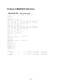
Contents
Main Index
Appendix E: Data Files For Example Problems
Down Previous
<< Back
Page
Chapter
Topics
Help
Next Page
Page
Up Page
Return
* ENTER A SCALING FACTOR BETWEEN 0.05 AND 1 TO SIZE THE PLOT:
*
(1= MAXIMUM SIZE POSSIBLE FOR OUTPUT DEVICE)
@RESPONSE: HELP LABEL = 2.1.53A
1
E-17
Exit
Exit