Download Manual - Group of Computational Hydrosystems

Processing Modflow
A Simulation System for Modeling Groundwater Flow and Pollution
Wen-Hsing Chiang and Wolfgang Kinzelbach
December 1998
Contents
Preface
1. Introduction . . . . . . . . . . . . . . . . . . . . . . . . . . . . . . . . . . . . . . . . . . . 1
System Requirements . . . . . . . . . . . . . . . . . . . . . . . . . . . . . . . . . . . . . . . . . . . . . . . . . .
Setting Up PMWIN . . . . . . . . . . . . . . . . . . . . . . . . . . . . . . . . . . . . . . . . . . . . . . . . . . .
Documentation . . . . . . . . . . . . . . . . . . . . . . . . . . . . . . . . . . . . . . . . . . . . . . . . . . . . . . .
Online Help . . . . . . . . . . . . . . . . . . . . . . . . . . . . . . . . . . . . . . . . . . . . . . . . . . . . . . . . .
4
4
4
5
2. Your First Groundwater Model with PMWIN . . . . . . . . . . . . . . . . 7
2.1 Run a Steady-State Flow Simulation . . . . . . . . . . . . . . . . . . . . . . . . . . . . . . . . . . . 8
2.2 Simulation of Solute Transport . . . . . . . . . . . . . . . . . . . . . . . . . . . . . . . . . . . . . . 32
2.2.1 Perform Transport Simulation with MT3D . . . . . . . . . . . . . . . . . . . . . . . . 33
2.2.2 Perform Transport Simulation with MOC3D . . . . . . . . . . . . . . . . . . . . . . 39
2.3 Automatic Calibration . . . . . . . . . . . . . . . . . . . . . . . . . . . . . . . . . . . . . . . . . . . . 44
2.3.1 Perform Automatic Calibration with PEST . . . . . . . . . . . . . . . . . . . . . . . . 46
2.3.2 Perform Automatic Calibration with UCODE . . . . . . . . . . . . . . . . . . . . . . 49
2.4 Animation . . . . . . . . . . . . . . . . . . . . . . . . . . . . . . . . . . . . . . . . . . . . . . . . . . . . . 51
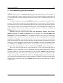
3. The Modeling Environment . . . . . . . . . . . . . . . . . . . . . . . . . . . . . 53
3.1 The Grid Editor . . . . . . . . . . . . . . . . . . . . . . . . . . . . . . . . . . . . . . . . . . . . . . . . . 55
3.2 The Data Editor . . . . . . . . . . . . . . . . . . . . . . . . . . . . . . . . . . . . . . . . . . . . . . . . . 59
3.2.1 The Cell-by-Cell Input Method . . . . . . . . . . . . . . . . . . . . . . . . . . . . . . . . . 61
3.2.2 The Zone Input Method . . . . . . . . . . . . . . . . . . . . . . . . . . . . . . . . . . . . . . 62
3.2.3 Specification of Data for Transient Simulations . . . . . . . . . . . . . . . . . . . . . 63
3.3 The File Menu . . . . . . . . . . . . . . . . . . . . . . . . . . . . . . . . . . . . . . . . . . . . . . . . . . 65
3.4 The Grid Menu . . . . . . . . . . . . . . . . . . . . . . . . . . . . . . . . . . . . . . . . . . . . . . . . . . 69
3.5 The Parameters Menu . . . . . . . . . . . . . . . . . . . . . . . . . . . . . . . . . . . . . . . . . . . . . 74
3.6 The Models Menu . . . . . . . . . . . . . . . . . . . . . . . . . . . . . . . . . . . . . . . . . . . . . . . 80
3.6.1 MODFLOW . . . . . . . . . . . . . . . . . . . . . . . . . . . . . . . . . . . . . . . . . . . . . . . 80
3.6.2 MOC3D . . . . . . . . . . . . . . . . . . . . . . . . . . . . . . . . . . . . . . . . . . . . . . . . . 111
3.6.3 MT3D . . . . . . . . . . . . . . . . . . . . . . . . . . . . . . . . . . . . . . . . . . . . . . . . . . 119
3.6.4 MT3DMS . . . . . . . . . . . . . . . . . . . . . . . . . . . . . . . . . . . . . . . . . . . . . . . 132
3.6.5 PEST (Inverse Modeling) . . . . . . . . . . . . . . . . . . . . . . . . . . . . . . . . . . . . 140
3.6.6 UCODE (Inverse Modeling) . . . . . . . . . . . . . . . . . . . . . . . . . . . . . . . . . .
3.6.7 PMPATH (Pathlines and Contours) . . . . . . . . . . . . . . . . . . . . . . . . . . . .
3.7 The Tools Menu . . . . . . . . . . . . . . . . . . . . . . . . . . . . . . . . . . . . . . . . . . . . . . . .
3.8 The Value Menu . . . . . . . . . . . . . . . . . . . . . . . . . . . . . . . . . . . . . . . . . . . . . . . .
3.9 The Options Menu . . . . . . . . . . . . . . . . . . . . . . . . . . . . . . . . . . . . . . . . . . . . . .
154
160
160
161
165
4. The Advective Transport Model PMPATH . . . . . . . . . . . . . . . . 175
4.1
4.2
4.3
4.4
The Semi-analytical Particle Tracking Method . . . . . . . . . . . . . . . . . . . . . . . . .
PMPATH Modeling Environment . . . . . . . . . . . . . . . . . . . . . . . . . . . . . . . . . . .
PMPATH Options Menu . . . . . . . . . . . . . . . . . . . . . . . . . . . . . . . . . . . . . . . . .
PMPATH Output Files . . . . . . . . . . . . . . . . . . . . . . . . . . . . . . . . . . . . . . . . . . .
176
180
187
195
5. Modeling Tools . . . . . . . . . . . . . . . . . . . . . . . . . . . . . . . . . . . . . . 199
5.1
5.2
5.3
5.4
5.5
5.6
The Digitizer . . . . . . . . . . . . . . . . . . . . . . . . . . . . . . . . . . . . . . . . . . . . . . . . . .
The Field Interpolator . . . . . . . . . . . . . . . . . . . . . . . . . . . . . . . . . . . . . . . . . . . .
The Field Generator . . . . . . . . . . . . . . . . . . . . . . . . . . . . . . . . . . . . . . . . . . . . .
The Results Extractor . . . . . . . . . . . . . . . . . . . . . . . . . . . . . . . . . . . . . . . . . . . .
The Water Balance Calculator . . . . . . . . . . . . . . . . . . . . . . . . . . . . . . . . . . . . .
The Graph Viewer . . . . . . . . . . . . . . . . . . . . . . . . . . . . . . . . . . . . . . . . . . . . . .
199
200
206
208
210
210
6. Examples and Applications . . . . . . . . . . . . . . . . . . . . . . . . . . . . 215
6.1 Tutorials . . . . . . . . . . . . . . . . . . . . . . . . . . . . . . . . . . . . . . . . . . . . . . . . . . . . . .
6.1.1 Tutorial 1 - Unconfined Aquifer System with Recharge . . . . . . . . . . . . .
6.1.2 Tutorial 2 - Confined and unconfined Aquifer System with River . . . . . .
6.2 Basic Flow Problems . . . . . . . . . . . . . . . . . . . . . . . . . . . . . . . . . . . . . . . . . . . .
6.2.1 Determination of Catchment Areas . . . . . . . . . . . . . . . . . . . . . . . . . . . . .
6.2.2 Use of the General-Head Boundary Condition . . . . . . . . . . . . . . . . . . . .
6.2.3 Simulation of a Two-layer Aquifer System in which the Top
Layer Converts between Wet and Dry . . . . . . . . . . . . . . . . . . . . . . . . . .
6.2.4 Simulation of a Water-table Mound resulting from Local Recharge . . . . .
6.2.5 Simulation of a Perched Water Table . . . . . . . . . . . . . . . . . . . . . . . . . . .
6.2.6 Simulation of an Aquifer System with Irregular Recharge and a Stream .
6.2.7 Simulation of a Flood in a River . . . . . . . . . . . . . . . . . . . . . . . . . . . . . . .
6.2.8 Simulation of Lakes . . . . . . . . . . . . . . . . . . . . . . . . . . . . . . . . . . . . . . . .
6.3 EPA Instructional Problems . . . . . . . . . . . . . . . . . . . . . . . . . . . . . . . . . . . . . . .
215
215
232
244
244
248
250
253
257
260
263
266
269
6.4 Automatic Calibration and Pumping Test . . . . . . . . . . . . . . . . . . . . . . . . . . . . . .
6.4.1 Basic Model Calibration Skill with PEST/UCODE . . . . . . . . . . . . . . . . .
6.4.2 Estimation of Pumping Rates . . . . . . . . . . . . . . . . . . . . . . . . . . . . . . . . .
6.4.3 The Theis Solution - Transient Flow to a Well in a Confined Aquifer . . .
6.4.4 The Hantush and Jacob Solution - Transient Flow to a Well in a
Leaky Confined Aquifer . . . . . . . . . . . . . . . . . . . . . . . . . . . . . . . . . . . . .
6.5 Geotechnical Problems . . . . . . . . . . . . . . . . . . . . . . . . . . . . . . . . . . . . . . . . . . .
6.5.1 Inflowof Water into an Excavation Pit . . . . . . . . . . . . . . . . . . . . . . . . . .
6.5.2 Flow Net and Seepage under a Weir . . . . . . . . . . . . . . . . . . . . . . . . . . .
6.5.3 Seepage Surface through a Dam . . . . . . . . . . . . . . . . . . . . . . . . . . . . . . .
6.5.4 Cutoff Wall . . . . . . . . . . . . . . . . . . . . . . . . . . . . . . . . . . . . . . . . . . . . . .
6.5.5 Compaction and Subsidence . . . . . . . . . . . . . . . . . . . . . . . . . . . . . . . . . .
6.6 Solute Transport . . . . . . . . . . . . . . . . . . . . . . . . . . . . . . . . . . . . . . . . . . . . . . .
6.6.1 One-Dimensional Dispersive Transport . . . . . . . . . . . . . . . . . . . . . . . . . .
6.6.2 Two-Dimensional Transport in a Uniform Flow Field . . . . . . . . . . . . . . .
6.6.3 Benchmark Problems and Application Examples from Liturature . . . . . . .
6.7 Miscellaneous Topics . . . . . . . . . . . . . . . . . . . . . . . . . . . . . . . . . . . . . . . . . . . .
6.7.1 Using the Field Interpolator . . . . . . . . . . . . . . . . . . . . . . . . . . . . . . . . . .
6.7.2 An Example of Stochastic Modeling . . . . . . . . . . . . . . . . . . . . . . . . . . . .
270
270
274
276
279
282
282
284
286
289
292
295
295
297
300
302
302
306
7. Appendices . . . . . . . . . . . . . . . . . . . . . . . . . . . . . . . . . . . . . . . . . 309
Appendix 1: Limitation of PMWIN . . . . . . . . . . . . . . . . . . . . . . . . . . . . . . . . . . . . . .
Appendix 2: Files and Formats . . . . . . . . . . . . . . . . . . . . . . . . . . . . . . . . . . . . . . . . . .
Appendix 3: Input Data Files of the Supported Models . . . . . . . . . . . . . . . . . . . . . . .
Appendix 4: Internal Data Files of PMWIN . . . . . . . . . . . . . . . . . . . . . . . . . . . . . . . .
Appendix 5: Using PMWIN with your MODFLOW . . . . . . . . . . . . . . . . . . . . . . . . .
Appendix 6: Running MODPATH with PMWIN . . . . . . . . . . . . . . . . . . . . . . . . . . . .
8. References
300
310
315
318
324
326
. . . . . . . . . . . . . . . . . . . . . . . . . . . . . . . . . . . . . . . . . 327
Preface
Welcome to Processing Modflow: A Simulation System for Modeling Groundwater Flow and
Pollution. Processing Modflow was originally developed for a remediation project of a disposal
site in the coastal region of Northern Germany. At the beginning of the work, the code was
designed as a pre- and postprocessor for the groundwater flow model MODFLOW. Several years
ago, we began to prepare a Windows-version of Processing Modflow with the goal of bringing
various codes together in a complete simulation system. The size of the program code grew, as
we began to prepare the Windows-based advective transport model PMPATH and add options
and features for supporting the solute transport models MT3D, MT3DMS and MOC3D and the
inverse models PEST and UCODE.
As in the earlier versions of Processing Modflow, our goal is to provide an integrated
groundwater modeling system with the hope that the very user-friendly implementation will lower
the threshold which inhibits the widespread use of computer based groundwater models. To
facilitate the use of Processing Modflow, more than 60 documented ready-to-run models are
included in this software. Some of these models deal with theoretical background, some of them
are of practical values.
The present text can be divided into three parts. The first two chapters introduce PMWIN
with an example. Chapters 3 through 5 are a detalied description of the building blocks. Chapter
3 describes the use of Processing Modflow; chapter 4 describes the advection model PMPATH
and chapter 5 introduces the modeling tools provided by Processing Modflow. The third part,
Chapter 6, provides two tutorials and documents the examples.
Beside this text, we have gathered about 3,000 pages of documents related to the supported
models. It is virtually not possible to provide all the documents in a printed form. So we decided
to present these documents in an electronic format. The advantage of the electronic documents
is considerable: with a single CD-ROM, you always have all necessary documents with you and
we save resources by saving valuable papers and trees.
Many many people contributed to this modeling system. The authors wish to express heartfelt
thanks to researchers and scientists, who have developed and coded the simulation programs
MODFLOW, MOC3D, MT3D, MT3DMS, PEST and UCODE. Without their contributions,
Processing Modflow would never have its present form. Many thanks are also due to authors of
numerous add-on packages to MODFLOW.
We wish to thank many of our friends and colleagues for their contribution in developing,
checking and validating the various parts of this software. We are very grateful to Steve
Bengtson, John Doherty, Maciek Lubczynski, Wolfgang Schäfer, Udo Quek, Axel Voss and
Jinhui Zhang who tested the software and provided many valuable comments and criticisms. For
their encouragement and support, we thank Ian Callow, Lothar Moosmann, Renate Taugs, Gerrit
van Tonder and Ray Volker. The authors also wish to thank Alpha Robinson, a scientist at the
University of Paderborn, who checked Chapter 3 of this user’s guide. And thanks to our readers
and software users - it is not possible for us to list by name here all the readers and users who
have made useful suggestions; we are very grateful for these.
Wen-Hsing Chiang @ Wolfgang Kinzelbach
Hamburg @ Zürich
December 1998
Processing Modflow
1
1. Introduction
The applications of MODFLOW, a modular three-dimensional finite-difference groundwater
model of the U. S. Geological Survey, to the description and prediction of the behavior of
groundwater systems have increased significantly over the last few years. The “original” version
of MODFLOW-88 (McDonald and Harbaugh, 1988) or MODFLOW-96 (Harbaugh and
McDonald, 1996a, 1996b) can simulate the effects of wells, rivers, drains, head-dependent
boundaries, recharge and evapotranspiration. Since the publication of MODFLOW various codes
have been developed by numerous investigators. These codes are called packages, models or
sometimes simply programs. Packages are integrated with MODFLOW, each package deals with
a specific feature of the hydrologic system to be simulated, such as wells, recharge or river.
Models or programs can be stand-alone codes or can be integrated with MODFLOW. A standalone model or program communicates with MODFLOW through data files. The advective
transport model PMPATH (Chiang and Kinzelbach, 1994, 1998), the solute transport model
MT3D (Zheng, 1990), MT3DMS (Zheng and Wang, 1998) and the parameter estimation
programs PEST (Doherty et al., 1994) and UCODE (Poeter and Hill, 1998) use this approach.
The solute transport model MOC3D (Konikow et al., 1996) and the inverse model MODFLOWP
(Hill, 1992) are integrated with MODFLOW. Both codes use MODFLOW as a function for
calculating flow fields.
This text and the companion software Processing Modflow for Windows (PMWIN) offer a
totally integrated simulation system for modeling groundwater flow and transport processes with
MODFLOW-88, MODFLOW-96, PMPATH, MT3D, MT3DMS, MOC3D, PEST and UCODE.
PMWIN comes with a professional graphical user-interface, the supported models and
programs and several other useful modeling tools. The graphical user-interface allows you to
create and simulate models with ease and fun. It can import DXF- and raster graphics and handle
models with up to 1,000 stress periods, 80 layers and 250,000 cells in each model layer. The
modeling tools include a Presentation tool, a Result Extractor, a Field Interpolator, a Field
Generator, a Water Budget Calculator and a Graph Viewer. The Result Extractor allows the
user to extract simulation results from any period to a spread sheet. You can then view the results
or save them in ASCII or SURFER-compatible data files. Simulation results include hydraulic
heads, drawdowns, cell-by-cell flow terms, compaction, subsidence, Darcy velocities,
concentrations and mass terms. The Field Interpolator takes measurement data and interpolates
the data to each model cell. The model grid can be irregularly spaced. The Water Budget
Calculator not only calculates the budget of user-specified zones but also the exchange of flows
between such zones. This facility is very useful in many practical cases. It allows the user to
determine the flow through a particular boundary. The Field Generator generates fields with
1. Introduction
2
Processing Modflow
heterogeneously distributed transmissivity or hydraulic conductivity values. It allows the user to
statistically simulate effects and influences of unknown small-scale heterogeneities. The Field
Generator is based on Mejía's (1974) algorithm. The Graph Viewer displays temporal
development curves of simulation results including hydraulic heads, drawdowns, subsidence,
compaction and concentrations.
Using the Presentation tool, you can create labelled contour maps of input data and
simulation results. You can fill colors to modell cells containing different values and report-quality
graphics may be saved to a wide variety of file formats, including SURFER, DXF, HPGL and
BMP (Windows Bitmap). The Presention tool can even create and display two dimensional
animation sequences using the simulation results (calculated heads, drawdowns or concentration).
At present, PMWIN supports seven additional packages, which are integrated with the
“original” MODFLOW. They are Time-Variant Specified-Head (CHD1), Direct Solution (DE45),
Density (DEN1), Horizontal-Flow Barrier (HFB1), Interbed-Storage (IBS1), Reservoir (RES1)
and Streamflow-Routing (STR1). The Time-Variant Specified-Head package (Leake et al., 1991)
was developed to allow constant-head cells to take on different values for each time step. The
Direct Solution package (Harbaugh, 1995) provides a direct solver using Gaussian elimination
with an alternating diagonal equation numbering scheme. The Density package (Schaars and van
Gerven, 1997) was designed to simulate the effect of density differences on the groundwater flow
system. The Horizontal-Flow Barrier package (Hsieh and Freckleton, 1992) simulates thin,
vertical low-permeability geologic features (such as cut-off walls) that impede the horizontal flow
of ground water. The Interbed-Storage package (Leake and Prudic, 1991) simulates storage
changes from both elastic and inelastic compaction in compressible fine-grained beds due to
removal of groundwater. The Reservoir package (Fenske et al., 1996) simulates leakage between
a reservoir and an underlying ground-water system as the reservoir area expands and contracts
in response to changes in reservoir stage. The Streamflow-Routing package (Prudic, 1988) was
designed to account for the amount of flow in streams and to simulate the interaction between
surface streams and groundwater.
The particle tracking model PMPATH uses a semi-analytical particle tracking scheme
(Pollock, 1988) to calculate the groundwater paths and travel times. PMPATH allows a user to
perform particle tracking with just a few clicks of the mouse. Both forward and backward particle
tracking schemes are allowed for steady-state and transient flow fields. PMPATH calculates and
displays pathlines or flowlines and travel time marks simultaneously. It provides various on-screen
graphical options including head contours, drawdown contours and velocity vectors.
The MT3D transport model uses a mixed Eulerian-Lagrangian approach to the solution of
the three-dimensional advective-dispersive-reactive transport equation. MT3D is based on the
assumption that changes in the concentration field will not affect the flow field significantly. This
1. Introduction
Processing Modflow
3
allows the user to construct and calibrate a flow model independently. After a flow simulation is
complete, MT3D simulates solute transport by using the calculated hydraulic heads and various
flow terms saved by MODFLOW. MT3D can be used to simulate changes in concentration of
single species miscible contaminants in groundwater considering advection, dispersion and some
simple chemical reactions. The chemical reactions included in the model are limited to equilibriumcontrolled linear or non-linear sorption and first-order irreversible decay or biodegradation.
MT3DMS is a further development of MT3D. The abbreviation MS denotes the MultiSpecies structure for accommodating add-on reaction packages. MT3DMS includes three major
classes of transport solution techniques, i.e., the standard finite difference method; the particle
tracking based Eulerian-Lagrangian methods; and the higher-order finite-volume TVD method.
In addition to the explicit formulation of MT3D, MT3DMS includes an implicit iterative solver
based on generalized conjugate gradient (GCG) methods. If this solver is used, dispersion,
sink/source, and reaction terms are solved implicitly without any stability constraints.
The MOC3D transport model computes changes in concentration of a single dissolved
chemical constituent over time that are caused by advective transport, hydrodynamic dispersion
(including both mechanical dispersion and diffusion), mixing or dilution from fluid sources, and
mathematically simple chemical reactions, including decay and linear sorption represented by a
retardation factor. MOC3D uses the method of characteristics to solve the transport equation on
the basis of the hydraulic gradients computed with MODFLOW for a given time step. This
implementation of the method of characteristics uses particle tracking to represent advective
transport and explicit finite-difference methods to calculate the effects of other processes. For
improved efficiency, the user can apply MOC3D to a subgrid of the primary MODFLOW grid that
is used to solve the flow equation. However, the transport subgrid must have uniform grid spacing
along rows and columns. Using MODFLOW as a built-in function, MOC3D can be modified to
simulate density-driven flow and transport.
The purpose of PEST and UCODE is to assist in data interpretation and in model calibration.
If there are field or laboratory measurements, PEST and UCODE can adjust model parameters
and/or excitation data in order that the discrepancies between the pertinent model-generated
numbers and the corresponding measurements are reduced to a minimum. Both codes do this by
taking control of the model (MODFLOW) and running it as many times as is necessary in order
to determine this optimal set of parameters and/or excitations.
1. Introduction
4
Processing Modflow
System Requirements
Hardware
Personal computer running Microsoft Windows 95/98 or Windows NT 4.0 or above.
16 MB of available memory (32MB or more highly recommended).
A CD-ROM drive and a hard disk.
VGA or higher-resolution monitor.
Microsoft Mouse or compatible pointing device.
Software
A FORTRAN compiler is required if you intend to modify and compile the models
MODFLOW-88, MODFLOW-96, MOC3D, MT3D or MT3DMS. For the reason of compability,
the models must be compiled by a Lahey Fortran compiler. The source codes of the abovementioned models are saved in the folder \Source\ of the CD-ROM.
Setting Up PMWIN
You install PMWIN on your computer using the self-installing program PM32010.EXE contained
in the folder \programs\pm5\ of the CD-ROM. Please note: If you are using Windows NT 4.0,
you must install the Service Pack 3 (or above) before installing PMWIN. Refer to the file
readme.txt on the PM5 CD-ROM for more information.
Documentation
The folder \Document\ of the CD-ROM contains electronic documents in the Portable Document
Format (PDF). You must first install the Acrobat® Reader before you can read or print the PDF
documents. You can find the installation file of the Acrobat® Reader in the folder \Reader\.
Execute the file \Reader\win95\ar302.exe from the CD directly and follow the screen to install
the Reader.
Starting PMWIN
Once you have completed the installation procedure, you can start Processing Modflow by using
the Start button on the task bar in Windows.
1. Introduction
Processing Modflow
5
Online Help
The online help system references nearly all aspects of PMWIN. You can access Help through the
Help menu Contents command, by searching for specific topics with the Help Search tool, or by
clicking the Help button to get context sensitive Help.
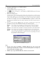
Help Search
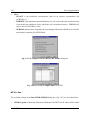
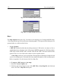
The fastest way to find a particular topic in Help is to use the Search dialog box. To display the
Search dialog box, either choose Search from the Help menu or click the Search button on any
Help topic screen.
< To search Help
1. From the Help menu, choose Search. (You can also click the Search button from any Help
topic window).
2. In the Search dialog box, type a word, or select one from the list by scrolling up or down.
Press ENTER or choose Show Topics to display a list of topics related to the word you
specified.
3. Select a topic and press ENTER or choose Go To to view the topic.
Context-Sensitive Help
Many parts of the PMWIN Help facility are context-sensitive. Context-sensitive means you can
access help on any part of PMWIN directly by clicking the Help button or by pressing the F1 key.
Updates
Today the development of groundwater modeling techniques is progressing very rapidly, and a
groundwater model must periodically be updated and expanded. For updates of PMWIN and our
other software you may access the following web-pages on the Internet:
http://www.uovs.ac.za/igs/index.htm
http://www.baum.ethz.ch./ihw/soft/welcome.html
1. Introduction
6
FOR YOUR NOTES
1. Introduction
Processing Modflow
Processing Modflow
7
2. Your First Groundwater Model with PMWIN
It takes just a few minutes to build your first groundwater flow model with PMWIN. First,
create a groundwater model by choosing New Model from the File menu. Next, determine the
size of the model grid by choosing Mesh Size from the Grid menu. Then, specify the geometry
of the model and set the model parameters, such as hydraulic conductivity, effective porosity
etc.. Finally, perform the flow simulation by choosing MODFLOW<
<Run... from the Models
menu.
After completing the flow simulation, you can use the modeling tools provided by PMWIN
to view the results, to calculate water bugdets of particular zones, or graphically display the
results, such as head contours. You can also use PMPATH to calculate and save pathlines or use
the finite difference transport models MT3D or MOC3D to simulate transport processes.
This chapter provides an overview of the modeling process with PMWIN, describes the
basic skills you need to use PMWIN, and takes you step by step through a sample problem. A
complete reference for all menus and dialog boxes in PMWIN is contained in Chapter 3. The
advective transport model PMPATH and the modeling tools are described in Chapter 4 and
Chapter 5, respectively.
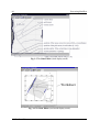
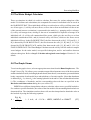
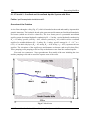
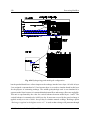
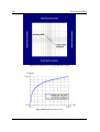
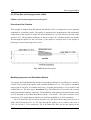
Overview of the Sample Problem
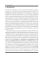
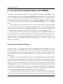
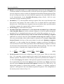
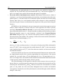
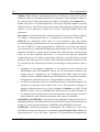
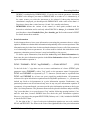
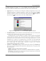
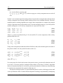
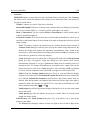
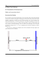
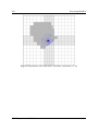
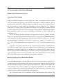
As shown in Fig. 2.1, an aquifer system with two stratigraphic units is bounded by no-flow
boundaries on the North and South sides. The West and East sides are bounded by rivers, which
are in full hydraulic contact with the aquifer and can be considered as fixed-head boundaries. The
hydraulic heads on the west and east boundaries are 9 m and 8 m above reference level,
respectively.
The aquifer system is unconfined and isotropic. The horizontal hydraulic conductivities of
the first and second stratigraphic units are 0.0001 m/s and 0.0005 m/s, respectively. Vertical
hydraulic conductivity of both units is assumed to be 10 percent of the horizontal hydraulic
conductivity. The effective porosity is 25 percent. The elevation of the ground surface (top of the
first stratigraphic unit) is 10m. The thickness of the first and the second units is 4 m and 6 m,
respectively. A constant recharge rate of 8×10-9 m/s is applied to the aquifer. A contaminated
area lies in the first unit next to the west boundary. The task is to isolate the contaminated area
using a fully penetrating pumping well located next to the eastern boundary.
A numerical model has to be developed for this site to calculate the required pumping rate
of the well. The pumping rate must be high enough, so that the contaminated area lies within the
Your First Groundwater Model with PMWIN
8
Processing Modflow
capture zone of the pumping well. We will use PMWIN to construct the numerical model and
use PMPATH to compute the capture zone of the pumping well. Based on the calculated
groundwater flow field, we will use MT3D and MOC3D to simulate the contaminant transport.
We will show how to use PEST and UCODE to calibrate the flow model and finally we will
create an animation sequence displaying the development of the contaminant plume.
To demonstrate the use of the transport models, we assume that the pollutant is dissolved
into groundwater at a rate of 1×10-4 µg/s/m 2. The longitudinal and transverse dispersivities of the
aquifer are 10m and 1m, respectively. The retardation factor is 2. The initial concentration,
molecular diffusion coefficient, and decay rate are assumed to be zero. We will calculate the
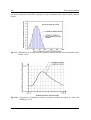
concentration distribution after a simulation time of 3 years and display the breakthrough curves
(concentration versus time) at two points [X, Y] = [290, 310], [390, 310] in both units.
Fig. 2.1 Configuration of the sample problem
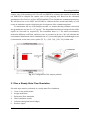
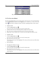
2.1 Run a Steady-State Flow Simulation
Six main steps must be performed in a steady-state flow simulation:
1. Create a new model model
2. Assign model data
3. Perform the flow simulation
4. Check simulation results
5. Calculate subregional water budget
6. Produce output
2.1 Run a Steady-State Flow Simulation
Processing Modflow
9
Step 1: Create a New Model
The first step in running a flow simulation is to create a new model.
<
1.
2.
To create a new model
Choose New Model from the File menu. A New Model dialog box appears. Select a folder
for saving the model data, such as C:\PM5DATA\SAMPLE, and type the file name
SAMPLE for the sample model. A model must always have the file extension .PM5. All file
names valid under Windows 95/98/NT with up to 120 characters can be used. It is a good
idea to save every model in a separate folder, where the model and its output data will be
kept. This will also allow you to run several models simultaneously (multitasking).
Click OK.
PMWIN takes a few seconds to create the new model. The name of the new model name is
shown in the title bar.
Step 2: Assign Model Data
The second step in running a flow simulation is to generate the model grid (mesh), specify
boundary conditions, and assign model parameters to the model grid.
PMWIN requires the use of consistent units throughout the modeling process. For
example, if you are using length [L] units of meters and time [T] units of seconds, hydraulic
conductivity will be expressed in units of [m/s], pumping rates will be in units of [m3/s] and
dispersivities will be in units of [m].
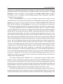
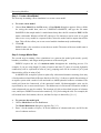
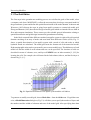
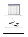
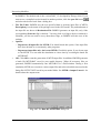
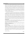
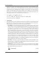
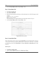
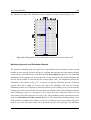
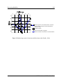
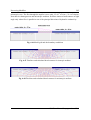
In MODFLOW, an aquifer system is replaced by a discretized domain consisting of an array
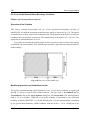
of nodes and associated finite difference blocks (cells). Fig. 2.2 shows a spatial discretization of
an aquifer system with a mesh of cells and nodes at which hydraulic heads are calculated. The
nodal grid forms the framework of the numerical model. Hydrostratigraphic units can be
represented by one or more model layers. The thicknesses of each model cell and the width of
each column and row may be variable. The locations of cells are described in terms of columns,
rows, and layers. PMWIN uses an index notation [J, I, K] for locating the cells. For example, the
cell located in the 2nd column, 6th row, and the first layer is denoted by [2, 6, 1].
<
1.
2.
To generate the model grid
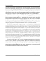
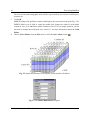
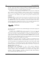
Choose Mesh Size from the Grid menu.
The Model Dimension dialog box appears (Fig. 2.3).
Enter 3 for the number of layers, 30 for the numbers of columns and rows, and 20 for the
size of columns and rows.
2.1 Run a Steady-State Flow Simulation
10
3.
4.
Processing Modflow
The first and second stratigraphic units will be represented by one and two model layers,
respectively.
Click OK.
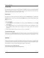
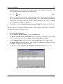
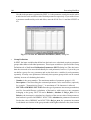
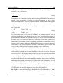
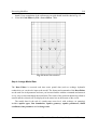
PMWIN changes the pull-down menus and displays the generated model grid (Fig. 2.4).
PMWIN allows you to shift or rotate the model grid, change the width of each model
column or row, or to add/delete model columns or rows. For our sample problem, you do
not need to modify the model grid. See section 3.1 for more information about the Grid
Editor.
Choose Leave Editor from the File menu or click the leave editor button
Fig. 2.2 Spatial discretization of an aquifer system and the cell indices
Fig. 2.3 The Model Dimension dialog box
2.1 Run a Steady-State Flow Simulation
.
Processing Modflow
11
Fig. 2.4 The generated model grid
Fig. 2.5 The Layer Options dialog box and the layer type drop-down list
The next step is to specify the type of layers.
< To assign the type of layers
1. Choose Layer Type from the Grid menu.
A Layer Options dialog box appears.
2.1 Run a Steady-State Flow Simulation
12
Processing Modflow
2.
Click a cell of the Type column, a drop-down button will appear within the cell. By clicking
the drop-down button, a list containing the avaliable layer types (Fig. 2.5) will be displayed.
Select 1: Unconfined for the first layer and 0: Confined for the other layers then click OK
to close the dialog box.
3.
As transmissivity and leakance are - by default - assumed to be calculated (see Fig. 2.5) from
conductivities and geometrical properties, the primary input variables to be specified are
horizontal and vertical hydraulic conductivities.
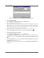
Now, you must specify basic boundary conditions of the flow model. The basic boundary
contition array (IBOUND array) contains a code for each model cell which indicates whether (1)
the hydraulic head is computed (active variable-head cell or active cell), (2) the hydraulic head
is kept fixed at a given value (fixed-head cell or time-varying specified-head cell), or (3) no flow
takes place within the cell (inactive cell). Use 1 for an active cell, -1 for a constant-head cell, and
0 for an inactive cell. For the sample problem, we need to assign -1 to the cells on the west and
east boundaries and 1 to all other cells.
<
1.
To assign the boundary condition to the flow model
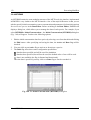
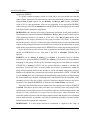
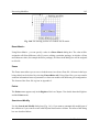
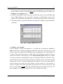
Choose Boundary Condition < IBOUND (Modflow) from the Grid Menu.
The Data Editor of PMWIN appears with a plan view of the model grid (Fig. 2.6). The grid
cursor is located at the cell [1, 1, 1], that is the upper-left cell of the first layer. The value of
the current cell is shown at the bottom of the status bar. The default value of the IBOUND
array is 1. The grid cursor can be moved horizontally by using the arrow keys or by clicking
the mouse on the desired position. To move to an other layer, use PgUp or PgDn keys or
click the edit field in the tool bar, type the new layer number, and then press enter.
Note that a DXF-map is loaded by using the Maps Options. See Chapter 3 for details.
2.
3.
Press the right mouse button. PMWIN shows a Cell Value dialog box.
Type -1 in the dialog box, then click OK.
The upper-left cell of the model has been specified to be a fixed-head cell.
4.
Now turn on duplication by clicking the duplication button
5.
.
Duplication is on, if the relief of the duplication button is sunk. The current cell value will
be duplicated to all cells passed by the grid cursor, if it is moved while duplication is on.
You can turn off duplication by clicking the duplication button again.
Move the grid cursor from the upper-left cell [1, 1, 1] to the lower-left cell [1, 30, 1] of the
model grid.
2.1 Run a Steady-State Flow Simulation
Processing Modflow
13
6.
7.
The value of -1 is duplicated to all cells on the west side of the model.
Move the grid cursor to the upper-right cell [30, 1, 1].
Move the grid cursor from the upper-right cell [30, 1, 1] to the lower-right cell [30, 30, 1].
The value of -1 is duplicated to all cells on the east side of the model.
8.
Turn on layer copy by clicking the layer copy button
9.
.
Layer copy is on, if the relief of the layer copy button is sunk. The cell values of the current
layer will be copied to other layers, if you move to the other model layer while layer copy is
on. You can turn off layer copy by clicking the layer copy button again.
Move to the second layer and then to the third layer by pressing the PgDn key twice.
The cell values of the first layer are copied to the second and third layers.
10. Choose Leave Editor from the File menu or click the leave editor button
.
Fig. 2.6 Data Editor with a plan view of the model grid.
The next step is to specify the geometry of the model.
< To specify the elevation of the top of model layers
1. Choose Top of Layers (TOP) from the Grid menu.
PMWIN displays the model grid.
2. Choose Reset Matrix... from the Value menu (or press Ctrl+R).
A Reset Matrix dialog box appears.
3. Enter 10 in the dialog box, then click OK.
2.1 Run a Steady-State Flow Simulation
14
Processing Modflow
4.
5.
The elevation of the top of the first layer is set to 10.
Move to the second layer by pressing PgDn.
Repeat steps 2 and 3 to set the top elevation of the second layer to 6 and the top elevation
of the third layer to 3.
6.
Choose Leave Editor from the File menu or click the leave editor button
<
1.
2.
To specify the elevation of the bottom of model layers
Choose Bottom of Layers (BOT) from the Grid menu.
Repeat the same procedure as described above to set the bottom elevation of the first,
second and third layers to 6, 3 and 0, respectively.
3.
Choose Leave Editor from the File menu or click the leave editor button
.
.
We are going to specify the temporal and spatial parameters of the model. The spatial parameters
for sample problem include the initial hydraulic head, horizontal and vertical hydraulic
conductivities and effective porosity.
<
1.
2.
3.
To specify the temporal parameters
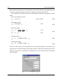
Choose Time... from the Parameters menu.
A Time Parameters dialog box will come up. The temporal parameters include the time
unit and the numbers of stress periods, time steps and transport steps. In MODFLOW, the
simulation time is divided into stress periods - i.e., time intervals during which all external
excitations or stresses are constant - which are, in turn, divided into time steps. In most
transport models, each flow time step is further divided into smaller transport steps. The
length of stress periods is not relevant to a steady state flow simulation. However, as we
want to perform contaminant transport simulation with MT3D and MOC3D, the actual time
length must be specified in the table.
Enter 9.46728E+07 (seconds) for Length of the first period.
Click OK to accept the other default values.
Now, you need to specify the initial hydraulic head for each model cell. The initial hydraulic head
at a fixed-head boundary will be kept constant during the flow simulation. The other heads are
starting values in a transient simulation or first guesses for the iterative solver in a steady-state
simulation. Here we firstly set all values to 8 and then correct the values on the west side by
overwriting them with a value of 9.
<
To specify the initial hydraulic head
2.1 Run a Steady-State Flow Simulation
Processing Modflow
1.
15
3.
4.
Choose Initial Hydraulic Heads from the Parameters menu.
PMWIN displays the model grid.
Choose Reset Matrix... from the Value menu (or press Ctrl+R) and enter 8 in the dialog
box, then click OK.
Move the grid cursor to the upper-left model cell.
Press the right mouse button and enter 9 into the Cell Value dialog box, then click OK.
5.
Now turn on duplication by clicking the duplication button
2.
6.
7.
8.
.
Duplication is on, if the relief of the duplication button is sunk. The current cell value will
be duplicated to all cells passed over by the grid cursor, if duplication is on.
Move the grid cursor from the upper-left cell to the lower-left cell of the model grid.
The value of 9 is duplicated to all cells on the west side of the model.
Turn on layer copy by clicking the layer copy button
.
Layer copy is on, if the relief of the layer copy button is sunk. The cell values of the current
layer will be copied to another layer, if you move to the other model layer while layer copy
is on.
Move to the second layer and the third layer by pressing PgDn twice.
The cell values of the first layer are copied to the second and third layers.
9.
Choose Leave Editor from the File menu or click the leave editor button
<
1.
2.
5.
To specify the horizontal hydraulic conductivity
Choose Horizontal Hydraulic Conductivity from the Parameters menu.
Choose Reset Matrix... from the Value menu (or press Ctrl+R), type 0.0001 in the dialog
box, then click OK.
Move to the second layer by pressing PgDn.
Choose Reset Matrix... from the Value menu (or press Ctrl+R), type 0.0005 in the dialog
box, then click OK.
Repeat steps 3 and 4 to set the value of the third layer to 0.0005.
6.
Choose Leave Editor from the File menu or click the leave editor button
<
1.
2.
To specify the vertical hydraulic conductivity
Choose Vertical Hydraulic Conductivity from the Parameters menu.
Choose Reset Matrix... from the Value menu (or press Ctrl+R), type 0.00001 in the dialog
box, then click OK.
Move to the second layer by pressing PgDn.
Choose Reset Matrix... from the Value menu (or press Ctrl+R), type 0.00005 in the dialog
3.
4.
3.
4.
.
.
2.1 Run a Steady-State Flow Simulation
16
Processing Modflow
5.
box, then click OK.
Repeat steps 3 and 4 to set the value of the third layer to 0.00005.
6.
Choose Leave Editor from the File menu or click the leave editor button
<
1.
To specify the effective porosity
Choose Effective Porosity from the Parameters menu.
Because the standard value is the same as the prescribed value of 0.25, you may leave the
editor and save the changes.
2.
Choose Leave Editor from the File menu or click the leave editor button
<
1.
2.
To specify the recharge rate
Choose MODFLOW<
< Recharge from the Models menu.
Choose Reset Matrix... from the Value menu (or press Ctrl+R), enter 8E-9 for Recharge
Flux [L/T] in the dialog box, then click OK.
3.
Choose Leave Editor from the File menu or click the leave editor button
.
.
.
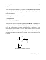
The last step before performing the flow simulation is to specify the location of the pumping well
and its pumping rate. In MODFLOW, an injection or pumping well is represented by a node (or
a cell). The user specifies an injection or pumping rate for each node. It is implicitly assumed that
the well penetrates the full thickness of the cell. MODFLOW can simulate the effects of pumping
from a well that penetrates more than one aquifer or layer provided that the user supplies the
pumping rate for each layer. The total pumping rate for the multilayer well is equal to the sum of
the pumping rates from the individual layers. The pumping rate for each layer ( Qk ) can be
approximately calculated by dividing the total pumping rate ( Qtotal ) in proportion to the layer
transmissivities (McDonald and Harbaugh, 1988):
Qk ' Qtotal @
Tk
ET
(2.1)
where Tk is the transmissivity of layer k and ET is the sum of the transmissivities of all layers
penetrated by the multilayer well. Unfortunately, as the first layer is unconfined, we do not
exactly know the saturated thickness and the transmissivity of this layer at the position of the
well. Eq. 2.1 cannot be used unless we assume a saturated thickness for calculating the
transmissivity. An other possibility to simulate a multi-layer well is to set a very large vertical
hydraulic conductivity (or vertical leakance), e.g. 1 m/s, to all cells of the well. The total
pumping rate is assigned to the lowest cell of the well. For the display purpose, a very small
pumping rate (say, 1×10-10 m3/s) can be assigned to other cells of the well. In this way, the exact
2.1 Run a Steady-State Flow Simulation
Processing Modflow
17
extraction rate from each penetrated layer will be calculated by MODFLOW implicitly and the
value can be obtained by using the Water Budget Calculator (see below).
As we do not know the required pumping rate for capturing the contaminated area shown
in Fig. 2.1, we will try a total pumping rate of 0.0012 m3/s.
<
1.
2.
3.
4.
5.
6.
7.
To specify the pumping well and the pumping rate
Choose MODFLOW<
<Well from the Models menu.
Move the grid cursor to the cell [25, 15, 1]
Press the right mouse button and type -1E-10, then click OK. Note that a negative value is
used to indicate a pumping well.
Move to the second layer by pressing PgDn.
Press the right mouse button and type -1E-10 then click OK.
Move to the third layer by pressing PgDn.
Press the right mouse button and type -0.0012 then click OK.
8.
Choose Leave Editor from the File menu or click the leave editor button
.
Step 3: Perform the Flow Simulation
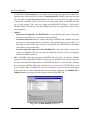
< To perform the flow simulation
1. Choose MODFLOW<
<Run... from the Models menu.
The Run Modflow dialog box appears (Fig. 2.7).
2. Click OK to start the flow computation.
Prior to running MODFLOW, PMWIN will use the user-specified data to generate input
files for MODFLOW (and optionally MODPATH) as listed in the table of the Run
Modflow dialog box. An input file will be generated only if the generate flag is set to .
You can click on the button to toggle the generate flag between and . Generally, you
do not need to change the flags, as PMWIN will care about the settings.
Step 4: Check Simulation Results
During a flow simulation, MODFLOW writes a detailed run record to the listing file
path\OUTPUT.DAT, where path is the folder in which your model data are saved. If a flow
simulation is successfully completed, MODFLOW saves the simulation results in various
unformatted (binary) files as listed in Table 2.1. Prior to running MODFLOW, the user may
control the output of these unformatted (binary) files by choosing Modflow<
<Output Control
from the Models menu. The output file path\INTERBED.DAT will only be generated, if the
Interbed Storage Package is activated (see Chapter 3 for details about the Interbed Storage
Package).
2.1 Run a Steady-State Flow Simulation
18
Processing Modflow
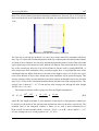
To check the quality of the simulation results, MODFLOW calculates a volumetric water
budget for the entire model at the end of each time step, and saves it in the file output.dat (see
Table 2.2). A water budget provides an indication of the overall acceptability of the numerical
solution. In numerical solution techniques, the system of equations solved by a model actually
consists of a flow continuity statement for each model cell. Continuity should also exist for the
total flows into and out of the entire model or a sub-region. This means that the difference
between total inflow and total outflow should equal to 0 (steady-state flow simulation) or to the
total change in storage (transient flow simulation). It is recommended to check the record file or
at least take a glance at it. The record file contains other further essential information. In case of
difficulties, this supplementary information could be very helpful.
Fig. 2.7 The Run Modflow dialog box
2.1 Run a Steady-State Flow Simulation
Processing Modflow
19
Table 2.1 Output files from MODFLOW
File
Contents
path\OUTPUT.DAT
Detailed run record and simulation report
path\HEADS.DAT
Hydraulic heads
path\DDOWN.DAT
Drawdowns, the difference between the starting heads and the
calculated hydraulic heads.
path\BUDGET.DAT
Cell-by-Cell flow terms
path\INTERBED.DAT
Subsidence of the entire aquifer and compaction and
preconsolidation heads in individual layers.
Interface file to MT3D/MT3DMS. This file is created by the LKMT
package provided by MT3D/MT3DMS (Zheng, 1990, 1998).
- path is the folder in which the model data are saved.
path\MT3D.FLO
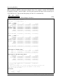
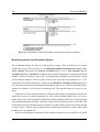
Table 2.2 Volumetric budget for the entire model written by MODFLOW
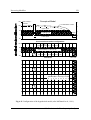
VOLUMETRIC BUDGET FOR ENTIRE MODEL AT END OF TIME STEP 1 IN STRESS PERIOD 1
----------------------------------------------------------------------------CUMULATIVE VOLUMES
-----------------IN:
--CONSTANT HEAD =
WELLS =
RECHARGE =
TOTAL IN =
L**3
RATES FOR THIS TIME STEP
------------------------
L**3/T
209690.3590
0.0000
254472.9380
IN:
--CONSTANT HEAD =
WELLS =
RECHARGE =
2.2150E-03
0.0000
2.6880E-03
464163.3130
TOTAL IN =
4.9030E-03
OUT:
---CONSTANT HEAD =
WELLS =
RECHARGE =
350533.6880
113604.0310
0.0000
OUT:
---CONSTANT HEAD =
WELLS =
RECHARGE =
3.7027E-03
1.2000E-03
0.0000
TOTAL OUT =
464137.7190
TOTAL OUT =
4.9027E-03
IN - OUT =
25.5938
IN - OUT =
2.7008E-07
PERCENT DISCREPANCY =
0.01
PERCENT DISCREPANCY =
0.01
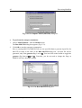
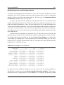
Step 5: Calculate subregional water budget
There are situations in which it is useful to calculate water budgets for various subregions of the
model. To facilitate such calculations, flow terms for individual cells are saved in the file
path\BUDGET.DAT. These individual cell flows are referred to as cell-by-cell flow terms, and
are of four types: (1) cell-by-cell stress flows, or flows into or from an individual cell due to one
of the external stresses (excitations) represented in the model, e.g., pumping well or recharge;
(2) cell-by-cell storage terms, which give the rate of accumulation or depletion of storage in an
2.1 Run a Steady-State Flow Simulation
20
Processing Modflow
individual cell; (3) cell-by-cell constant-head flow terms, which give the net flow to or from
individual fixed-head cells; and (4) internal cell-by-cell flows, which are the flows across
individual cell faces-that is, between adjacent model cells. The Water Budget Calculator uses
the cell-by-cell flow terms to compute water budgets for the entire model, user-specified
subregions, and flows between adjacent subregions.
<
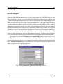
1.
3.
4.
5.
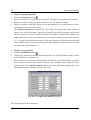
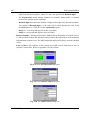
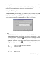
To calculate subregional water budgets
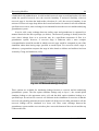
Choose Water Budget from the Tools menu.
A Water Budget dialog box appears (Fig. 2.8). For a steady-state flow simulation, you do
not need to change the settings in the Time group.
Click Zones.
A zone is a subregion of a model for which a water budget will be calculated. A zone is
indicated by a zone number ranging from 0 to 50. A zone number must be assigned to each
model cell. The zone number 0 indicates that a cell is not associated with any zone. Follow
steps 3 to 5 to assign zone numbers 1 to the first and 2 to the second layer.
Choose Reset Matrix... from the Value menu, type 1 in the dialog box, then click OK.
Press PgDn to move to the second layer.
Choose Reset Matrix... from the Value menu, type 2 in the dialog box, then click OK.
6.
Choose Leave Editor from the File menu or click the leave editor button
7.
Click OK in the Water Budget dialog box.
2.
.
Fig. 2.8 The Water Budget dialog box
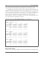
PMWIN calculates and saves the flows in the file path\WATERBDG.DAT as shown in Table
2.3. The unit of the flows is [L3T-1]. Flows are calculated for each zone in each layer and each
time step. Flows are considered IN, if they are entering a zone. Flows between subregions are
given in a Flow Matrix. HORIZ. EXCHANGE gives the flow rate horizontally across the
boundary of a zone. EXCHANGE (UPPER) gives the flow rate coming from (IN) or going to
(OUT) to the upper adjacent layer. EXCHANGE (LOWER) gives the flow rate coming from
2.1 Run a Steady-State Flow Simulation
Processing Modflow
21
(IN) or going to (OUT) to the lower adjacent layer. For example, consider EXCHANGE
(LOWER) of ZONE=1 and LAYER=1, the flow rate from the first layer to the second layer is
2.587256E-03 m3/s. The percent discrepancy in Table 2.3 is calculated by
100 @ (IN & OUT)
Table
Output from
(IN 2.3
% OUT)
/ 2 the Water Budget Calculator
(2.2)
FLOWS ARE CONSIDERED "IN" IF THEY ARE ENTERING A SUBREGION
THE UNIT OF THE FLOWS IS [L^3/T]
TIME STEP
1 OF STRESS PERIOD
1
ZONE=
1 LAYER= 1
FLOW TERM
IN
OUT
IN-OUT
STORAGE 0.0000000E+00 0.0000000E+00 0.0000000E+00
CONSTANT HEAD 1.8407618E-04 2.4361895E-04 -5.9542770E-05
HORIZ. EXCHANGE 0.0000000E+00 0.0000000E+00 0.0000000E+00
EXCHANGE (UPPER) 0.0000000E+00 0.0000000E+00 0.0000000E+00
EXCHANGE (LOWER) 0.0000000E+00 2.5872560E-03 -2.5872560E-03
WELLS 0.0000000E+00 1.0000000E-10 -1.0000000E-10
DRAINS 0.0000000E+00 0.0000000E+00 0.0000000E+00
RECHARGE 2.6880163E-03 0.0000000E+00 2.6880163E-03
.
.
.
.
.
.
.
.
SUM OF THE LAYER 2.8720924E-03 2.8308749E-03 4.1217543E-05
.
.
.
.
.
.
.
.
ZONE= 2 LAYER= 2
FLOW TERM
IN
OUT
IN-OUT
STORAGE 0.0000000E+00 0.0000000E+00 0.0000000E+00
CONSTANT HEAD 1.0027100E-03 1.7383324E-03 -7.3562248E-04
HORIZ. EXCHANGE 0.0000000E+00 0.0000000E+00 0.0000000E+00
EXCHANGE (UPPER) 2.5872560E-03 0.0000000E+00 2.5872560E-03
EXCHANGE (LOWER) 0.0000000E+00 1.8930938E-03 -1.8930938E-03
WELLS 0.0000000E+00 1.0000000E-10 -1.0000000E-10
DRAINS 0.0000000E+00 0.0000000E+00 0.0000000E+00
RECHARGE 0.0000000E+00 0.0000000E+00 0.0000000E+00
.
.
.
.
.
.
.
.
SUM OF THE LAYER 3.5899659E-03 3.6314263E-03 -4.1460386E-05
-------------------------------------------------------------.
.
.
.
.
.
.
.
WATER BUDGET OF SELECTED ZONES:
IN
OUT
IN-OUT
ZONE( 1): 2.8720924E-03 2.8308751E-03 4.1217310E-05
ZONE( 2): 3.5899659E-03 3.6314263E-03 -4.1460386E-05
-------------------------------------------------------------WATER BUDGET OF THE WHOLE MODEL DOMAIN:
FLOW TERM
IN
OUT
IN-OUT
STORAGE 0.0000000E+00 0.0000000E+00 0.0000000E+00
CONSTANT HEAD 2.2149608E-03 3.7026911E-03 -1.4877303E-03
WELLS 0.0000000E+00 1.2000003E-03 -1.2000003E-03
DRAINS 0.0000000E+00 0.0000000E+00 0.0000000E+00
RECHARGE 2.6880163E-03 0.0000000E+00 2.6880163E-03
.
.
.
.
.
.
.
.
-------------------------------------------------------------SUM 4.9029770E-03 4.9026916E-03 2.8545037E-07
DISCREPANCY [%] 0.01
The value of the element (i,j) of the following flow matrix gives the flow
rate from the i-th zone into the j-th zone. Where i is the column
index and j is the row index.
FLOW MATRIX:
1
2
.............................
0 1
0.0000
0.0000
0 2
2.5873E-03 0.0000
2.1 Run a Steady-State Flow Simulation
22
Processing Modflow
In this example, the percent discrepancy of in- and outflows for the model and each zone in each
layer is acceptably small. This means the model equations have been correctly solved.
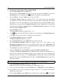
To calculate the exact flow rates to the well, we repeat the previous procedure for
calculating subregional water budgets. This time we only assign the cell [25, 15, 1] to zone 1, the
cell [25, 15, 2] to zone 2 and the cell [25, 15, 3] to zone 3. All other cells are assigned to zone
0. The water budget is shown in Table 2.4. The pumping well is extracting 7.7992809E-05 m3/s
from the first layer, 5.603538E-04 m3/s from the second layer and 5.5766129E-04 m3/s
from the third layer. Almost all water withdrawn comes from the second stratigraphic unit, as
can be expected from the configuration of the aquifer.
Table 2.4 Output from the Water Budget Calculator for the pumping well
FLOWS ARE CONSIDERED "IN" IF THEY ARE ENTERING A SUBREGION
THE UNIT OF THE FLOWS IS [L^3/T]
TIME STEP
1 OF
ZONE= 1 LAYER=
FLOW TERM
STORAGE
CONSTANT HEAD
HORIZ. EXCHANGE
EXCHANGE (UPPER)
EXCHANGE (LOWER)
WELLS
DRAINS
RECHARGE
.
.
SUM OF THE LAYER
.
.
ZONE= 2 LAYER=
FLOW TERM
STORAGE
CONSTANT HEAD
HORIZ. EXCHANGE
EXCHANGE (UPPER)
EXCHANGE (LOWER)
WELLS
.
.
SUM OF THE LAYER
ZONE=
3 LAYER=
FLOW TERM
STORAGE
CONSTANT HEAD
HORIZ. EXCHANGE
EXCHANGE (UPPER)
EXCHANGE (LOWER)
WELLS
.
.
SUM OF THE LAYER
STRESS PERIOD
1
IN
0.0000000E+00
0.0000000E+00
7.7992809E-05
0.0000000E+00
0.0000000E+00
0.0000000E+00
0.0000000E+00
3.1999998E-06
.
.
8.1192811E-05
.
.
2
IN
0.0000000E+00
0.0000000E+00
5.6035380E-04
7.9696278E-05
0.0000000E+00
0.0000000E+00
.
.
6.4005010E-04
1
OUT
IN-OUT
0.0000000E+00 0.0000000E+00
0.0000000E+00 0.0000000E+00
0.0000000E+00 7.7992809E-05
0.0000000E+00 0.0000000E+00
7.9696278E-05 -7.9696278E-05
1.0000000E-10 -1.0000000E-10
0.0000000E+00 0.0000000E+00
0.0000000E+00 3.1999998E-06
.
.
.
.
7.9696380E-05 1.4964317E-06
.
.
.
.
OUT
IN-OUT
0.0000000E+00 0.0000000E+00
0.0000000E+00 0.0000000E+00
0.0000000E+00 5.6035380E-04
0.0000000E+00 7.9696278E-05
6.4027577E-04 -6.4027577E-04
1.0000000E-10 -1.0000000E-10
.
.
.
.
6.4027589E-04 -2.2578752E-07
3
IN
0.0000000E+00
0.0000000E+00
5.5766129E-04
6.4027577E-04
0.0000000E+00
0.0000000E+00
.
.
1.1979371E-03
OUT
IN-OUT
0.0000000E+00 0.0000000E+00
0.0000000E+00 0.0000000E+00
0.0000000E+00 5.5766129E-04
0.0000000E+00 6.4027577E-04
0.0000000E+00 0.0000000E+00
1.2000001E-03 -1.2000001E-03
.
.
.
.
1.2000001E-03 -2.0629959E-06
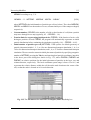
Step 6: Produce Output
In addition to the water budget, PMWIN provides various possibilities for checking simulation
2.1 Run a Steady-State Flow Simulation
Processing Modflow
23
results and creating graphical outputs. Pathlines and velocity vectors can be displayed by
PMPATH. Using the Results Extractor, simulation results of any layer and time step can be
read from the unformatted (binary) result files and saved in ASCII Matrix files. An ASCII Matrix
file contains a value for each model cell in a layer. PMWIN can load ASCII matrix files into a
model grid. The format of the ASCII Matrix file is described in Appendix 2. In the following, we
will carry out the steps:
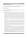
1. Use the Results Extractor to read and save the calculated hydraulic heads.
2. Generate a contour map based on the calculated hydraulic heads for the first layer.
3. Use PMPATH to compute pathlines as well as the capture zone of the pumping well.
<
1.
2.
3.
4.
5.
6.
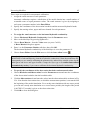
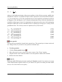
7.
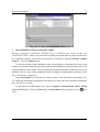
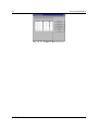
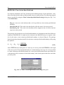
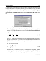
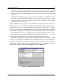
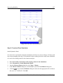
To read and save the calculated hydraulic heads
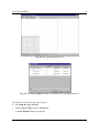
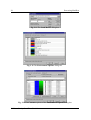
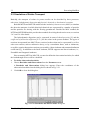
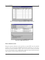
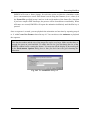
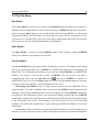
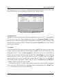
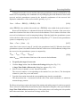
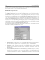
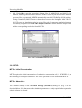
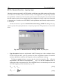
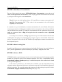
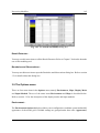
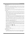
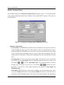
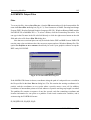
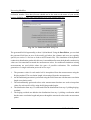
Choose Results Extractor... from the Tools menu
The Results Extractor dialog box appears (Fig. 2.9). The options in the Results Extractor
dialog box are grouped under four tabs - MODFLOW, MOC3D, MT3D and MT3DMS. In
the MODFLOW tab, you may choose a result type from the Result Type drop-down box.
You may specify the layer, stress period and time step from which the result should be
read. The spreadsheet displays a series of columns and rows. The intersection of a row and
column is a cell. Each cell of the spreadsheet corresponds to a model cell in a layer. Refer to
Chap. 5 for more detailed information about the Results Extractor. For the current sample
problem, follow steps 2 to 6 to save the hydraulic heads of each layer in three ASCII Matrix
files.
Choose Hydraulic Head from the Result Type drop-down box.
Type 1 in the Layer edit field.
For the current problem (steady-state flow simulation with only one stress period and one
time step), the stress period and time step number should be 1.
Click Read.
Hydraulic heads in the first layer at time step 1 and stress period 1 will be read and put into
the spreadsheet. You can scroll the spreadsheet by clicking on the scrolling bars next to the
spreadsheet.
Click Save.
A Save Matrix As dialog box appears. By setting the Save as type option, the result can
be optionally saved as an ASCII matrix or a SURFER data file. Specify the file name
H1.DAT and select a folder in which H1.DAT should be saved. Click OK when ready.
Repeat steps 3, 4 and 5 to save the hydraulic heads of the second and third layer in the files
H2.DAT and H3.DAT, respectively.
Click Close to close the dialog box.
2.1 Run a Steady-State Flow Simulation
24
Processing Modflow
<
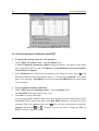
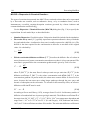
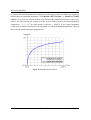
1.
To generate contour maps of the calculated heads
Choose Presentation from the Tools menu
Data specified in Presentation will not be used by any parts of PMWIN. We can use
Presentation to save temporary data or to display simulation results graphically.
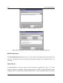
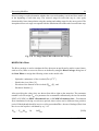
Choose Matrix... from the Value menu (or Press Ctrl+B).
The Browse Matrix dialog box appears (Fig. 2.10). Each cell of the spreadsheet
corresponds to a model cell in the current layer. You can load an ASCII Matrix file into the
spreadsheet or save the spreadsheet in an ASCII Matrix file by clicking Load or Save.
Alternatively, you may select the Results Extractor from the Value menu, read the head
results and use an additional Apply button in the Results Extractor dialog box to put the
data into the Presentation matrix.
Click the Load... button.
The Load Matrix dialog box appears (Fig. 2.11).
2.
3.
4.
5.
6.
7.
Click
and select the file H1.DAT, which was saved earlier by the Results Extractor.
Click OK when ready. H1.DAT is loaded into the spreadsheet.
In the Browse Matrix dialog box, click OK.
The Browse Matrix dialog box is closed.
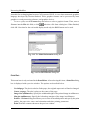
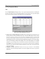
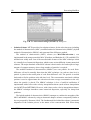
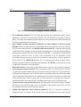
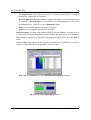
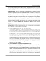
Choose Environment from the Options menu (or Press Ctrl+E).
The Environment Options dialog box appears (Fig. 2.12). The options in the
Environment Options dialog box are grouped under three tabs. Appearance and
Coordinate System allow the user to modify the appearance and position of the model grid.
Use Contours to generate contour maps.
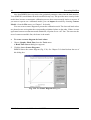
Click the Contours tab, check Visible, then click the Restore Defaults button.
Clicking on the Restore Defaults button, PMWIN sets the number of contour lines to 11
and uses the maxmum and minimum values in the current layer as the minimum and
maximum contour levels (Fig. 2.13). If Fill Contours is checked, the contours will be filled
with the colors given in the Fill column of the table. Use Label Format button to specify an
appropriate format.
Note that PMWIN will clear the Visible check box when you leave the Editor.
8.
In the Environment Options dialog box, Click OK.
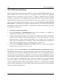
PMWIN will redraw the model and display the contours (Fig. 2.14).
9. To save or print the graphics, choose Save Plot As... or Print Plot... from the File menu.
10. Press PgDn to move to the second layer. Repeat steps 2 to 9 to load the file H2.DAT,
display and save the plot.
11. Choose Leave Editor from the File menu or click the leave editor button
2.1 Run a Steady-State Flow Simulation
and click Yes
Processing Modflow
25
to save changes to Presentation.
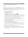
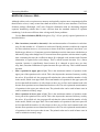
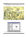
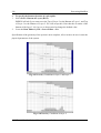
Using the procedure described above, you can generate contour maps based of your input data,
any kind of simulation results or any data saved as an ASCII Matrix file. For example, you can
create a contour map of the starting heads or you can use the Result Extractor to read the
concentration distribution and display the contours. You can also generate contour maps of the
fields created by the Field Interpolator or Field Generator. See chapter 5 for details about the
Field Interpolator and Field Generator.
Fig. 2.9 The Results Extractor dialog box.
Fig. 2.10 The Browse Matrix dialog box
2.1 Run a Steady-State Flow Simulation
26
Processing Modflow
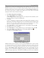
Fig. 2.11 The Load Matrix dialog box
Fig. 2.12 The Environment Options dialog box
Fig. 2.13 The Contours options of the Environment Options dialog box
2.1 Run a Steady-State Flow Simulation
Processing Modflow
27
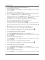
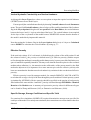
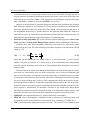
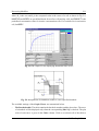
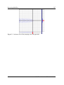
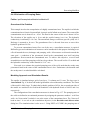
Fig. 2.14 A contour map of the hydraulic heads in the first layer
<
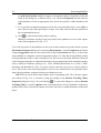
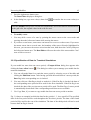
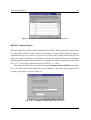
1.
To delineate the capture zone of the pumping well
Choose PMPATH (Pathlines and Contours) from the Models menu.
PMWIN calls the advective transport model PMPATH and the current model will be loaded
into PMPATH automatically. PMPATH uses a "grid cursor" to define the column and row
for which the cross-sectional plots should be displayed. You can move the grid cursor by
holding down the Ctrl-key and click the left mouse button on the desired position.
Note that if you subsequently modify and calculate a model within PMWIN, you must load the
modified model into PMPATH again to ensure that the modifications can be recognized by
PMPATH. To load a model, click
and select a model file with the extension .PM5 from the
Open Model dialog box.
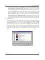
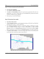
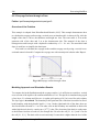
2. To calculate the capture zone of the pumping well:
a. Click the Set Particle button
b. Move the mouse cursor to the model area. The mouse cursor turns into crosshairs.
c. Place the crosshairs at the upper-left corner of the pumping well, as shown in Fig. 2.15.
d. Hold down the left moust button and drag the crosshairs until the window covers the
pumping well.
e. Release the left mouse button.
2.1 Run a Steady-State Flow Simulation
28
Processing Modflow
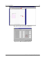
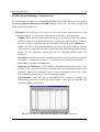
An Add New Particles dialog box appears. Assign the numbers of particles to the edit
fields in the dialog box as shown in Fig. 2.16. Click the Properties tab and click the
colored button to select an appropriate color for the new particles. When finished, click
OK.
f. To set particles around the pumping well in the second and third layer, press PgDn to
move down a layer and repeat steps c, d and e. Use other colors for the new particles in
the second and third layers.
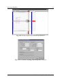
g. Click
to start the backward particle tracking.
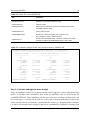
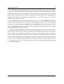
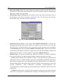
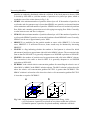
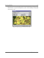
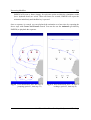
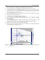
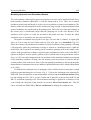
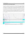
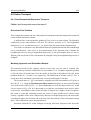
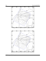
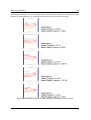
PMPATH calculates and shows the projections of the pathlines as well as the capture
zone of the pumping well (Fig. 2.17).
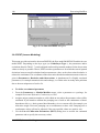
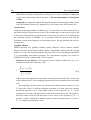
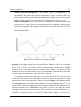
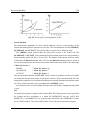
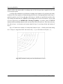
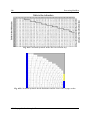
To see the projection of the pathlines on the cross-section windows in greater details, open an
Environment Options dialog box by choosing Environment... from the Options menu and set
a larger exaggeration value for the vertical scale in the Cross Sections tab. Fig. 2.18 shows the
same pathlines by setting the vertical exaggeration value to 10. Note that some pathlines end up
at the groundwater surface, where recharge occurs. This is one of the major differences between
a three-dimensional and a two-dimensional model. In two-dimensional areal simulation models,
such as ASM for Windows (Chiang et al., 1998), FINEM (Kinzelbach et al, 1990) or MOC
(Konikow and Bredehoeft, 1978), a vertical velocity term does not exist (or always equals to
zero). This leads to the result that pathlines can never be tracked back to the ground surface
where the groundwater recharge from the precipitation occurs.
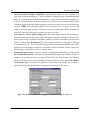
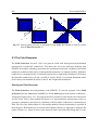
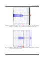
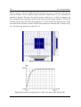
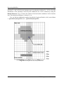
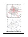
PMPATH can create time-related capture zones of pumping wells. The 100-days-capture
zone shown in Fig. 2.19 is created by using the settings in the Particle Tracking (Time)
Properties dialog box (Fig. 2.20) and clicking
. To open this dialog box, choose Particle
Tracking (Time)... from the Options menu. Note that because of lower hydraulic conductivity
(and thus lower flow velocity) the capture zone in the first layer is smaller than those in the other
layers.
2.1 Run a Steady-State Flow Simulation
Processing Modflow
29
Fig. 2.15 The sample model loaded in PMPATH
Fig. 2.16 The Add New Particles dialog box
2.1 Run a Steady-State Flow Simulation
30
Processing Modflow
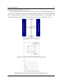
Fig. 2.17 The capture zone of the pumping well (with vertical exaggeration=1)
Fig. 2.18 The capture zone of the pumping well (with vertical exaggeration=10)
2.1 Run a Steady-State Flow Simulation
Processing Modflow
31
Fig. 2.19 100-days-capture zone calculated by PMPATH
Fig. 2.20 The Particle Tracking (Time) Properties dialog box
2.1 Run a Steady-State Flow Simulation
32
Processing Modflow
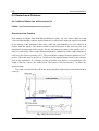
2.2 Simulation of Solute Transport
Basically, the transport of solutes in porous media can be described by three processes:
advection, hydrodynamic dispersion and physical, chemical or biochemical reactions.
Both the MT3D and MOC3D models use the method-of-characteristics (MOC) to simulate
the advection transport, in which dissolved chemicals are represented by a number of particles
and the particles are moving with the flowing groundwater. Besides the MOC method, the
MT3D and MT3DMS models provide other methods for solving the advective term, see sections
3.6.3 and 3.6.4 for details.
The hydrodynamic dispersion can be expressed in terms of the dispersivity [L] and the
coefficient of molecular diffusion [L2T-1] for the solute in the porous medium. The types of
reactions incorporated into MOC3D are restricted to those that can be represented by a firstorder rate reaction, such as radioactive decay, or by a retardation factor, such as instaneous,
reversible, sorption-desorption reactions goverened by a linear isotherm and constant distribution
coefficient (Kd). In addition to the linear isotherm, MT3D supports non-linear isotherms, i.e.,
Freundlich and Langmuir isotherms.
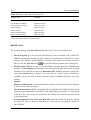
Prior to running MT3D or MOC3D, you need to define the observation boreholes, for which
the breakthrough curvers will be calculated.
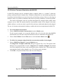
< To define observation boreholes
1. Choose Boreholes and Observations from the Paramters menu.
A Boreholes and Observations dialog box appears. Enter the coordinates of the
observation boreholes into the dialog box as shown in Fig. 2.21.
2. Click OK to close the dialog box.
Fig. 2.21 The Boreholes and Observations dialog box
The Modeling Environment - 3.1 The Grid Editor
Processing Modflow
33
2.2.1 Perform Transport Simulation with MT3D
MT3D requires a boundary condition code for each model cell which indicates whether (1)
solute concentration varies with time (active concentration cell), (2) the concentration is kept
fixed at a constant value (constant-concentration cell), or (3) the cell is an inactive concentration
cell. Use 1 for an active concentration cell, -1 for a constant-concentration cell, and 0 for an
inactive concentration cell. Active, variable-head cells can be treated as inactive concentration
cells to minimize the area needed for transport simulation, as long as the solute concentration is
insignificant near those cells.
Similar to the flow model, you must specify the initial concentration for each model cell. The
initial concentration at a constant-concentration cell will be kept constant during a transport
simulation. The other concentration are starting values in a transport simulation.
<
1.
To assign the boundary condition to MT3D
Choose Boundary Conditions < ICBUND (MT3D/MT3DMS) from the Grid menu.
For the current example, we accept the default value 1 for all cells.
2.
Choose Leave Editor from the File menu or click the leave editor button
<
1.
To set the initial concentration
Choose MT3D < Initial Concentration from the Models menu.
For the current example, we accept the default value 0 for all cells.
2.
Choose Leave Editor from the File menu or click the leave editor button
<
1.
2.
To assign the input rate of contaminants
Choose MT3D < Sink/Source Concentration < Recharge from the Models menu.
Assign 12500 [µg/m 3] to the cells within the contaminated area.
This value is the concentration associated with the recharge flux. Since the recharge rate is
8 × 10-9 [m3/m2/s] and the dissolution rate is 1 × 10-4 [µg/s/m 2], the concentration associated
with the recharge flux is 1 × 10-4 / 8 × 10-9 = 12500 [µg/m 3]
3.
Choose Leave Editor from the File menu or click the leave editor button
<
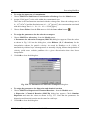
1.
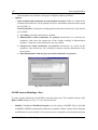
To assign the transport parameters to the Advection Package
Choose MT3D < Advection... from the Models menu.
An Advection Package (MTADV1) dialog box appears. Enter the values as shown in
Fig. 2.22 into the dialog box, select Method of Characteristics (MOC) for the solution
scheme and First-order Euler for the particle tracking algorithm.
.
.
.
2.2.1 Perform Transport Simulation with MT3D
34
2.
Processing Modflow
Click OK to close the dialog box.
Fig. 2.22 The Advection Package (MTADV1) dialog box
<
1.
2.
3.
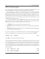
To assign the dispersion parameters
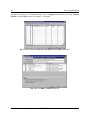
Choose MT3D < Dispersion... from the Models menu.
A Dispersion Package (MT3D) dialog box appears. Enter the ratios of the transverse
dispersivity to longitudinal dispersivity as shown in Fig. 2.23.
Click OK.
PMWIN displays the model grid. At this point you need to specify the longitudinal
dispersivity to each cell of the grid.
Choose Reset Matrix... from the Value menu (or press Ctrl+R), type 10 in the dialog box
then click OK.
4.
Turn on layer copy by clicking the layer copy button
5.
Move to the second layer and the third layer by pressing PgDn twice.
The cell values of the first layer are copied to the second and third layers.
6.
Choose Leave Editor from the File menu or click the leave editor button
<
1.
To assign the chemical reaction parameters
Choose MT3D < Chemical Reaction < Layer by Layer from the Models menu.
A Chemical Reaction Package (MTRCT1) dialog box appears. Clear the check box
Simulate the radioactive decay or biodegradation and select Linear equlibrium
2.2.1 Perform Transport Simulation with MT3D
.
.
Processing Modflow
35
isotherm for the type of sorption. For the linear isotherm, the retardation factor R for each
cell is calculated at the beginning of the simulation by
R ' 1 %
2.
Db
n
@ Kd
(2.3)
Where n [-] is the effective porosity with respect to the flow through the porous medium, Db
[ML-3] is the bulk density of the porous medium and Kd [L3M-1] is the distribution coefficient
of the solute in the porous medium. As the effective porosity is equal to 0.25, setting
Db = 2000 and Kd = 0.000125 yields R = 2.
Click OK to close the Chemical Reaction Package (MTRCT1) dialog box (Fig. 2.24).
The last step before running the transport model is to specify the output times, at which the
calculated concentration should be saved.
<
1.
2.
3.
To specify the output times
Choose MT3D < Output Control... from the Models menu.
An Output Control (MT3D, MT3DMS) dialog box appears. The options in this dialog
box are grouped under three tabs - Output Terms, Output Times and Misc.
Click the Output Times tab, then click the header Output Time of the (empty) table.
An Output Times dialog box appears. Enter 3000000 to Interval in this dialog box then
click OK to accept the other defalut values.
Click OK to close the Output Control (MT3D, MT3DMS) dialog box (Fig. 2.25).
Fig. 2.23 The Advection Package (MTADV1) dialog box
2.2.1 Perform Transport Simulation with MT3D
36
Processing Modflow
Fig. 2.24 The Chemical Reaction Package (MTRCT1) dialog box
Fig. 2.25 The Output Control (MT3D, MT3DMS) dialog box
<
1.
2.
To perform the transport simulation
Choose MT3D<
<Run... from the Models menu.
The Run MT3D/MT3D96 dialog box appears (Fig. 2.26).
Click OK to start the transport computation.
Prior to running MT3D, PMWIN will use user-specified data to generate input files for
MT3D as listed in the table of the Run MT3D/MT3D96 dialog box. An input file will be
generated, only if the generate flag is set to . You can click on the button to toggle the
generate flag between
and . Generally, you do not need to change the flags, as
PMWIN will care about the settings.
2.2.1 Perform Transport Simulation with MT3D
Processing Modflow
37
Fig. 2.26 The Run MT3D/MT3D96 dialog box
< Check simulation results and produce output
During a transport simulation, MT3D writes a detailed run record to the file
path\OUTPUT.MT3, where path is the folder in which your model data are saved. MT3D saves
the simulation results in various files, which can be controlled by choosing MT3D < Output
Control... from the Models menu.
To check the quality of the simulation results, a mass budget is calculated at the end of each
transport step and accumulated to provide summarized information on the total mass into or out
of the groundwater flow system. The discrepancy between the total mass in and out servers as an
indicator of the accuracy of the simulation results. It is highly recommended to check the record
file or at least take a glance at it.
Using Presentation you can generate contour maps of the calculated concentration. Fig.
2.27 shows the calculated concentration in the third layer at the end of the simulation (simulation
time=9.467E+07 seconds).
To generate the breakthrough curves, choose Graphs < Concentration Time < MT3D
from the Tools menu. Click on the Plot flags of the Boreholes table until they are set to (Fig.
2.28).
2.2.1 Perform Transport Simulation with MT3D
38
Processing Modflow
Fig. 2.27 Simulated concentration at 3 years in the third layer
Fig. 2.28 Concentration-time curves at the observation boreholes
2.2.1 Perform Transport Simulation with MT3D
Processing Modflow
39
2.2.2 Perform Transport Simulation with MOC3D
In MOC3D, transport may be simulated within a subgrid, which is a “window” within the
primary model grid used to simulate flow. Within the subgrid, the row and column spacing must
be uniform, but the thickness can vary from cell to cell and layer to layer. However, the range in
thickness values (or product of thickness and effective porosity) should be as small as possible.
The initial concentration must be specified throughout the subgrid within which solute
transport occurs. MOC3D assumes that the concentration outside of the subgrid is the same
within each layer, so only one value is specified for each layer within and adjacent to the subgrid.
The use of constant-concentration boundary condition has not been implemented in MOC3D.
<
1.
To set the initial concentration
Choose MOC3D < Initial Concentration from the Models menu.
For the current example, we accept the default value 0 for all cells. Note that PMWIN
automatically uses the same initial concentration values for both MOC3D and MT3D.
2.
Choose Leave Editor from the File menu or click the leave editor button
<
1.
To define the transport subgrid and the concentration outside of the subgrid
Choose MOC3D < Subgrid... from the Models menu.
The Subgrid for Transport (MOC3D) dialog box appears (Fig. 2.29). The options in the
dialog box are grouped under two tabs - Subgrid and C’ Outside of Subgrid. The default
size of the subgrid is the same as the model grid used to simulate flow. The default initial
concentration outside of the subgrid is zero. We will accept the defaults.
Click OK to accept the default values and close the dialog box.
2.
.
Fig. 2.29 The Subgrid for Transport (MOC3D) dialog box.
2.2.2 Perform Transport Simulation with MOC3D
40
Processing Modflow
<
1.
2.
To assign the input rate of contaminants
Choose MOC3D < Sink/Source Concentration < Recharge from the Models menu.
Assign 12500 [µg/m 3] to the cells within the contaminated area.
This value is the concentration associated with the recharge flux. Since the recharge rate is
8 × 10-9 [m3/m2/s] and the dissolution rate is 1 × 10-4 [µg/s/m 2], the concentration associated
with the recharge flux is 1 × 10-4 / 8 × 10-9 = 12500 [µg/m 3]
3.
Choose Leave Editor from the File menu or click the leave editor button
<
1.
To assign the parameters for the advective transport
Choose MOC3D < Advection... from the Models menu.
A Parameters for Advection Transport (MOC3D) dialog box appears. Enter the values
as shown in Fig. 2.30 into the dialog box, select Bilinear (X, Y directions) for the
interpolation scheme for particle velocity. As noted by Konikow et al. (1996), if
transmissivity within a layer is homogeneous or smoothly varying, bilinear interpolation of
velocity yields more realistic pathlines for a given discretization than does linear
interpolation.
Click OK to close the dialog box.
2.
.
Fig. 2.30 The Parameters for Advective Transport dialog box.
<
1.
2.
To assign the parameters for dispersion and chemical reaction
Choose MOC3D < Dispersion & Chemical Reaction... from the Models menu.
A Dispersion / Chemical Reaction (MOC3D) dialog box appears. Check Simulate
Dispersion and enter the values as shown in Fig. 2.31. Note that the parameters for
dispersion and chemical reaction are the same for each layer.
Click OK to close the dialog box.
2.2.2 Perform Transport Simulation with MOC3D
Processing Modflow
41
Fig. 2.31 The Dispersion / Chemical Reaction (MOC3D) dialog box.
<
1.
2.
3.
4.
To set Strong/Weak Flag
Choose MOC3D < Strong/Weak Flag from the Models menu.
Move the grid cursor to the cell [25, 15, 1].
Press the right mouse button and type 1, then click OK. Note that a strong sink or source is
indicated by the value of 1 in the matrix. When a fluid source is “strong”, new particles are
added to replace old particles as they are advected out of that cell. Where a fluid sink is
“strong”, particles are removed after they enter that cell.
Repeat steps 2 and 3 to assign the value 1 to the cells [25, 15, 2] and [25, 15, 3].
5.
Choose Leave Editor from the File menu or click the leave editor button
<
1.
To specify the output terms and times
Choose MOC3D < Output Control... from the Models menu.
An Output Control (MOC3D) dialog box appears. The options in the dialog box are
grouped under five tabs - Concentration, Velocity, Particle Locations, Disp. Coeff. and
Misc.
In the Concentration tab, select the option These data will be printed or saved every
Nth particle moves and enter N = 20.
Click OK to accept all other default values and close the Output Control (MOC3D) dialog
box (Fig. 2.32).
2.
3.
.
2.2.2 Perform Transport Simulation with MOC3D
42
Processing Modflow
Fig. 2.32 The Output Control (MOC3D) dialog box.
<
1.
2.
To perform the transport simulation
Choose MOC3D<
<Run... from the Models menu.
The Run MOC3D dialog box appears (Fig. 2.33).
Click OK to start the transport computation.
Prior to running MOC3D, PMWIN will use user-specified data to generate input files for
MOC3D as listed in the table of the Run MOC3D dialog box. An input file will be
generated, only if the generate flag is set to . You can click on the button to toggle the
generate flag between
and . Generally, you do not need to change the flags, as
PMWIN will care about the settings.
Fig. 2.33 The Run MOC3D dialog box
2.2.2 Perform Transport Simulation with MOC3D
Processing Modflow
43
< Check simulation results and produce output
During a transport simulation, MOC3D writes a detailed run record to the file
path\MOC3D.LST, where path is the folder in which your model data are saved. MOC3D saves
the simulation results in various files, which can be controlled by choosing MOC3D < Output
Control... from the Models menu.
To check the quality of the simulation results, mass balance calculations are performed and
saved in the run record file. The mass in storage at any time is calculated from the concentrations
at the nodes of the transport subgrid to provide summarized information on the total mass into
or out of the groundwater flow system. The mass balance error will typically exhibit an
oscillatory behavior over time, because of the finite-difference approximation and the nature of
the method of characteristics. As discussed in Konikow et al. (1996), as long as the oscillations
remain within a steady range, not exceeding about ±10 percent as a guide, then the error
probably does not represent a bias and is not a serious problem. Rather, the ocillations only
reflect the fact that the mass balance calculation is itself just an approximation.
Using Presentation you can generate contour maps of the calculated concentration. Fig.
2.34 shows the calculated concentration at 3 years in the third layer (simulation time=9.467E+07
seconds).
To generate the breakthrough curves, choose Graphs < Concentration Time < MOC3D
from the Tools menu. Click on the Plot flags of the Boreholes table until they are set as in Fig.
2.35.
Fig. 2.34 Simulated concentration at 3 years in the third layer
2.2.2 Perform Transport Simulation with MOC3D
44
Processing Modflow
Fig. 2.35 Concentration-time curves at the observation boreholes
2.3 Automatic Calibration
Calibration of a flow model is accomplished by finding a set of parameters, hydrologic stresses
or boundary conditions so that the simulated heads or drawdowns match the measurement values
to a reasonable degree. The calibration process is one of the most difficult and critical steps in
the model application. Hill (1998) gives methods and guidelines for model calibration using
inverse modeling.
To demonstrate the use of the inverse models PEST and UCODE within PMWIN, we
assume that the hydraulic conductivity in the third layer is homogeneous but its value is
unknown. We want to find out this value through a model calibration by using the measured
hydraulic heads at the observation boreholes listed below.
Borehole
X-coordinate
Y-coordinate
Layer
Hydraulic Head
1
130
200
3
8.85
2
200
400
3
8.74
3
480
250
3
8.18
4
460
450
3
8.26
2.3 Automatic Calibration
Processing Modflow
45
Three steps are required for an automatic calibration.
1. Assign the zonal structure of each parameter.
Automatic calibration requires a subdivision of the model domain into a small number of
reasonable zones of equal parameter values. The zonal structure is given by assigning to
each zone a parameter number in the Data Editor.
2. Specify the coordinates of the observation boreholes and the measured hydraulic heads.
3. Specify the starting values, upper and lower bounds for each parameter.
<
1.
2.
3.
4.
5.
To assign the zonal structure to the horizontal hydraulic conductivity
Choose Horizontal Hydraulic Conductivity from the Parameters menu.
Move to the third layer by pressing PgDn twice.
Choose Reset Matrix... from the Value menu (or press Ctrl+R).
A Reset Matrix dialog box appears.
Enter 1 to the Parameter Number edit box, then click OK.
The horizontal hydraulic conductivity of the third layer is set to the parameter #1.
Choose Leave Editor from the File menu or click the leave editor button
.
Note that for layers of type 0:confined and 2:confined/unconfined (transmissivity=const.),
MODFLOW reads transmissvity (instead of hydraulic conductivity) from the model data file,
consequently we are actually calibrating the transmissivity and must use suitable values for the
initial guess and lower and upper bounds. Change the layer type to 3:confined/unconfined
(transmissivity varies), if you want to calibrate the horizontal hydraulic conductivity.
<
1.
2.
3.
To specify the coordinates of the observation boreholes and measured values
Choose Boreholes and Observations from the Parameters menu and enter the coordinates
of the observation boreholes into the boreholes table.
Click the Observations tab and enter the values into the observations table as shown in Fig.
2.36. Note that the observation time, to which the measurement pertains, is measured from
the beginning of the model simulation. For a steady state simulation with one stress period
(you can run a steady state simulation over several stress periods), the length of the period
(9.46728E+07 seconds) is given as the observation time.
Click OK to close the dialog box.
2.3 Automatic Calibration
46
Processing Modflow
Fig. 2.36 The Boreholes and Observations dialog box
2.3.1 Perform Automatic Calibration with PEST
<
1.
2.
<
1.
2.
To specify the starting values for each parameter
Choose PEST < Parameter List... from the Models menu.
A List of Calibration Parameters (PEST) dialog box appears. The options of the dialog
box are grouped under five tabs - Parameters, Group Definitions, Prior Information,
Control Data and Options.
In the Parameters tab, activate the first parameter (by setting the Active flag to ) from
Parameters table and enter values shown in Fig. 2.37 into the table. PARVAL1 is the initial
guess of the parameter. PARLBUD is the lower bound and PARUBUD is the upper bound
of the parameter.
To perform the automatic calibration
Choose PEST (Inverse Modeling) < Run... from the Models menu.
The Run PEST dialog box appears (Fig. 2.38).
Click OK to start the calibration.
Prior to running PEST, PMWIN will use user-specified data to generate input files for PEST
and MODFLOW as listed in the table of the Run PEST dialog box. An input file will be
generated, only if the generate flag is set to . You can click on the button to toggle the
generate flag between
and . Generally, you do not need to change the flags, as
PMWIN will care about the settings.
2.3.1 Perform Automatic Calibration with PEST
Processing Modflow
47
Fig. 2.37 The List of Calibration Parameters (PEST) dialog box
Fig. 2.38 The Run PEST dialog box
Check calibration results
During the automatic calibration several result files are created. PEST writes the optimized
parameter values to the input files of MODFLOW (BCF.DAT, WEL.DAT, etc.) and creates a
detailed run record file path\PESTCTL.REC, where path is the folder in which your model data
are saved. The simulation results of MODFLOW are updated by using the optimized parameter
values, which are saved in a separate file PESTCTL.PAR.
2.3.1 Perform Automatic Calibration with PEST
48
Processing Modflow
Note that PMWIN does not retrieve the optimized parameter values into the data matrices.
Your (PMWIN-) model data will not be modified in any way. This provides more security for the
model data, because an automatic calibration process does not necessarily lead to a success. If
you want to operate on a calibrated model, you can import the model by choosing Convert
Model... from the File menu, see Chapter 3 for details.
You can create a scatter diagram to present the calibration result. The observed head values
are plotted on one axis against the corresponding calculated values on the other. If there is exact
agreement between measurement and simulation, all points lie on a 45° line. The narrower the
area of scatter around this line, the better is the match.
<
1.
2.
To create a scatter diagram for head values
Choose Graph < Head-Time from the Tools menu.
A Head-Time Curves dialog box appears.
Click the button Scatter Diagram »
PMWIN shows the scatter diagram (Fig. 2.39). See Chapter 5 for details about the use of
this dialog box.
Fig. 2.39 The Scatter Diagram dialog box
2.3.1 Perform Automatic Calibration with PEST
Processing Modflow
49
2.3.2 Perform Automatic Calibration with UCODE
<
1.
2.
3.
<
1.
2.
To specify the starting values for each parameter
Choose UCODE < Parameter List... from the Models menu.
A List of Calibration Parameters (UCODE) dialog box appears. The options of the
dialog box are grouped under five tabs - Parameters, Prior Information, Control Data
and Options.
In the Parameters tab, activate the first parameter (by setting the Active flag to ) from
Parameters table and enter values shown in Fig. 2.40 into the table. Start-value is the initial
guess of the parameter. Minimum is the reasonable minimum value and Maximum is the
reasonable maximum value for the parameter. These two values are used solely to determine
how the final optimized value of the parameter compares to a reasonable range of values.
Check the Log-transform flag to log-transform the parameter. This will ensure that only
positive values will be used for the parameter during the calibration.
To perform the automatic calibration
Choose UCODE (Inverse Modeling) < Run... from the Models menu.
The Run UCODE dialog box appears (Fig. 2.41).
Click OK to start the calibration.
Prior to running UCODE, PMWIN will use user-specified data to generate input files for
UCODE and MODFLOW as listed in the table of the Run UCODE dialog box. An input
file will be generated, only if the generate flag is set to . You can click on the button to
toggle the generate flag between and
as PMWIN will care about the settings.
. Generally, you do not need to change the flags,
Check calibration results
During the automatic calibration several result files are created. Similar to PEST, UCODE writes
the optimized parameter values to the input files of MODFLOW (BCF.DAT, WEL.DAT, etc.)
and creates a detailed run record file path\ucode._ot, where path is the folder in which your
model data are saved. The simulation results of MODFLOW are updated by using the optimized
parameter values, which are saved in a separate file ucode._st. Similar to PEST, you can create
a scatter diagram to present the calibration result (see above).
Note that PMWIN does not retrieve the optimized parameter values into the data matrices.
Your (PMWIN-) model data will not be modified in any way. This provides more security for the
model data, because an automatic calibration process does not necessarily lead to a success. If
2.3.2 Perform Automatic Calibration with UCODE
50
Processing Modflow
you want to operate on a calibrated model, you can import the model by choosing Convert
Model... from the File menu, see Chapter 3 for details.
Fig. 2.40 The List of Calibration Parameters (UCODE) dialog box
Fig. 2.41 The Run UCODE dialog box
2.3.2 Perform Automatic Calibration with UCODE
Processing Modflow
51
2.4 Animation
You already learned how to use the Presentation tool to create and print contour maps from
calculated head and concentration values. The saved or printed images are static and ideal for
paper-reports. In many cases, however, these static images cannot ideally illustrate motion of
concentration plumes or temporal variation of hydraulic heads or drawdowns. PMWIN provides
an animation technique to display a sequence of the saved images in rapid succession. Although
the animation process requires relatively large amount of computer resources to read, process
and display the data, the effect of a motion picture is often very helpful.
The Presentation tool is used to create animation sequences. The following steps show how to
use the Environment Options and Animation dialog boxes to create an animation sequence for
displaying the motion of the concentration plume in the third layer.
<
1.
2.
3.
4.
5.
6.
7.
8.
9.
To create an animation sequence
Choose Presentation from the Tools menu.
Move to the third layer by pressing PgDn twice.
Choose Environment... from the Options menu
Click the Contours tab, clear Display contour lines, and check Visible and Fill Colors.
Click the table header Level.
A Contour Levels dialog box appears. Set Minimum to 100, Maximum to 1600 and
Interval to 100. These values are used, because we already know the range of the
concentration values from Fig. 2.27. When finished, click OK to close the dialog box.
Click the table header Fill.
A Color Spectrum dialog box appears. Set an appropriate color range by clicking the
Minimum color and Maximum color buttons. When finished, click OK to close the dialog
box.
Click OK to close the Enviroment Options dialog box.
Choose Animation... from the File menu.
The Animation dialog box appears (Fig. 2.42).
Click the open file button
.
A Save File dialog box appears. Select or specify a file name in the dialog box, then click
Open.
10. Check Create New Frames, set Result Type to Concentration (MT3D) and set Display
Time (s) to 0.1. Display Time is the display duration for each frame.
11. In the Animation dialog box, click OK to start the animation.
2.4 Animation
52
Processing Modflow
PMWIN will create a frame (image) for each time point at which the simulation results
(here: concentration) are saved. Each frame is saved using the filenames fn.xxx, where fn is
the Frame File specified in step 9 and xxx is the serial number of the frame files. Note that
if you have complex DXF-basemaps, the process will be slowed down considerably. When
all frames are created, PMWIN will repeat the animation indefinitely until the Esc key is
pressed.
Once a sequence is created, you can playback the animation at a later time by repeating steps 8
to 11 with Create New Frames cleared in step 10. You can also use the Animator to playback
the sequence.
Note that the number and the size of the image files can be very large. Make sure that there is
enough free space on your hard disk. To reduce the file size, you can change the size of the
PMWIN window before creating the frames. You may turn off the display of the model grid
in the Environment Options dialog box so that you don’t have the grid cluttering the
animation.
Fig. 2.42 The Animation dialog box
2.4 Animation
Processing Modflow
53
3. The Modeling Environment
PMWIN requires the use of consistent units throughout the modeling process. For example, if
you are using length [L] units of meters and time [T] units of seconds, hydraulic conductivity will
be expressed in units of [m/s], pumping rates will be in units of [m3/s] and dispersivity will be in
units of [m].
A toolbar with buttons representing PMWIN operations or commands is displayed below
the menus. The toolbar is a shortcut for the pull-down menus. To execute one of these shortcuts,
move the mouse cursor over the toolbar button and click on it. In the following sections, the use
of the respective menus will be described in detail. Some of this information has already been
given in Chapter 2, however, this chapter is a complete reference of all menus and dialogs in
PMWIN, therefore some repetitions may occur.
PMWIN contains the following menus File, Grid, Parameters, Models, Tools, Value,
Options and Help. The Value and Options menus are available only in the Grid Editor and
Data Editor environment. PMWIN uses an intelligent menu system to help you control the
modeling process. If you have specified a model data set, the corresponding item of the Grid,
Parameters and Models menus will be checked. To deactivate a selected item in the Models
menu, just seleted the item again. If you do not know which model data still need to be specified,
you may try to run your model by selecting the menu item Run... from the corresponding model
in the Models menu. PMWIN will then tell you what parameters or model data are necessary to
run your model, if unspecified. An overview of the menus in PMWIN is given in table 3.1.
Most of the user-specified data are saved in binary files. A list of the internal data files of
PMWIN is given in Appendix 4. Prior to running the supported models MODFLOW, MT3D,
MT3DMS, MOC3D or the inverse models PEST and UCODE, PMWIN will generate the
required ASCII input files. The names of the ASCII input files are given in Appendix 3. The
formats of the input files of MODFLOW and MT3D, MT3DMS and MOC3D can be found in the
user’s guide the corresponding software on the companion CD-ROM. The particle tracking model
PMPATH retrieves the binary data files of PMWIN directly, thus no ASCII input file is required
by PMPATH.
3. The Modeling Environment
54
Processing Modflow
Table 3.1 An overview of the menus in PMWIN
Menu
Description
File
Create new models; open existing models; convert models to the PMWIN format; Save and
print plots.
Grid
Generate or modify the size of a model grid; input of the geometry of the aquifer.
Parameters
Input of spatial aquifer parameters, for example transmissivity; Input of temporal
parameters, for example simulation length or number of stress periods.
Models
Specify model-specific data using the module provided and call simulation programs. For
example, you can add wells, use the recharge or river modules to MODFLOW or define the
advection or dispersion parameters in MT3D. The simulation programs are called by
selecting Run... from the corresponding model.
Tools
Call the modeling tools.
Value
Manipulate model data; read or save model data in separate files.
Options
Modify the appearance of the model grid on the screen; Load site maps.
Help
Call the Help file.
3. The Modeling Environment
Processing Modflow
55
3.1 The Grid Editor
The first steps in the groundwater modeling process are to define the goals of the model, select
a computer code (here: MODFLOW), collect the necessary data, develop a conceptual model of
the groundwater system and define the spatial discretization of the model domain. Anderson and
Woessner (1992) discuss the steps in going from aquifer systems to a numerical model grid.
Zheng and Bennett (1995) describe the design of model grids which are intended for use both in
flow and transport simulations. These sources provide valuable general information relating to
spatial discretization and grid design in numerical groundwater modeling.
In the block-centered finite difference method, an aquifer system is replaced by a discretized
domain consisting of an array of nodes and associated finite difference blocks (cells). Fig. 3.1
shows a spatial discretization of an aquifer system with a mesh of cells and nodes at which
hydraulic heads are calculated. The nodal grid forms the framework of the numerical model.
Hydrostratigraphic units can be represented by one or more model layers. The thicknesses of each
model cell and the width of each column and row can be specified. The locations of cells are
described in terms of columns, rows, and layers. PMWIN uses an index notation [J, I, K] for
locating the cells. For example, the cell located in the 2nd column, 6th row, and the first layer is
denoted by [2, 6, 1].
Fig. 3.1 Spatial discretization of an aquifer system and the cell indices
To generate or modify a model grid, choose Mesh Size... from the Grid menu. If a grid does not
exist, a Model Dimension dialog box (Fig. 3.2) will allow you to specify the number of layers and
the numbers and the widths of columns and rows of the model grid. After specifying these data
3.1 The Grid Editor
56
Processing Modflow
and clicking the OK button, the Grid Editor shows a worksheet with a plan view of the model
grid (Fig. 3.3). Using the Environment Options dialog box (see section 3.9), you can adjust the
coordinate system, the extent of the worksheet and the positon of the model grid to fit the realworld coordinates of your study site. By default, the origin of the coordinate system is set at the
lower-left corner of the worksheet and the extent of the worksheet is set to twice that of the
model grid.
The first time you use the Grid Editor, you can insert or delete columns or rows (see
below). After leaving the Grid Editor and saving the grid, you can subsequently refine the
existing model grid by calling the Grid Editor again. In each case, you can change the size of any
column or row. If the grid is refined, all model parameters are retained. For example, if the cell
of a pumping well is divided into four cells, all four cells will be treated as wells and the sum of
their pumping rates will be kept the same as that of the previous single well. The same is true for
hydraulic conductance of the head-dependent boundaries, i.e., river, stream, drain and generalhead boundary. If the Stream-Routing Package is used, you must redefine the segment and reach
number of the stream.
<
To change the width of a column and/or a row
1.
Click the assign value button
2.
3.
4.
.
The grid cursor appears only if the Assign Value button is pressed down. You do not need
to click this button, if its relief is already sunk, ie, if it is already active.
Move the grid cursor to the desired cell by using the arrow keys or by clicking the mouse on
the desired position. The sizes of the current column and row are shown on the status bar.
Press the right mouse button once.
The Grid Editor shows a Size of Column and Row dialog box (Fig. 3.4).
In the dialog box, type new values, then click OK.
< To insert or delete a column and/or a row
Inserting or deleting columns/rows is only possible when using the Grid Editor for the first time.
1.
Click the assign value button
2.
Move the grid cursor to the desired cell by using the arrow keys or by clicking the mouse on
the desired position.
Hold down the Ctrl-key and press the up or right arrow key to insert a row or a column;.
press the down or left arrow key to delete the current row or column.
3.
.
< To refine a column and/or a row
Refining columns/rows is only possible when the grid has already been saved.
3.1 The Grid Editor
Processing Modflow
57
1.
Click the assign value button
2.
Move the grid cursor to the desired cell by using the arrow keys or by clicking the mouse on
the desired position.
Hold down the Ctrl-key and press the up or right arrow key to refine a row or a column;
press the down or left arrow key to remove the refinement. The refinements of a column or
a row are shown on the status bar.
3.
.
Fig. 3.2 The Model Dimension dialog box
Fig. 3.3 The Grid Editor
3.1 The Grid Editor
58
Processing Modflow
Fig. 3.4 The Size of Column and Row dialog box
The following table summarizes the use of the tool bar buttons of the Grid Editor.
Table 3.2 Summary of the tool bar buttons for the Grid Editor
Button
Action
leave editor; Leave the Grid Editor
assign value; Allows you to move the grid cursor and assign values
zoom in; Allows you to drag a zoom-window over a part of the model domain.
zoom out; Displays the entire worksheet.
rotate grid; To rotate the model grid, click the mouse on the worksheet and hold down the left button
while you move the mouse.
shift grid; To shift the model grid, click the mouse on the worksheet and hold down the left button
while you move the mouse.
duplication on/off; If duplication is turned on, the size of the current row or column will be copied
to all rows or columns passed by the grid cursor. Duplication is on, when the relief of the button is
sunk.
3.1 The Grid Editor
Processing Modflow
59
3.2 The Data Editor
The Data Editor is used to assign parameter values to the model cells. To start the Data Editor,
select a corresponding item from the Grid, Parameters or Models menu. For example, if you
want to assign horizontal hydraulic conductivity to model cells, you will choose Horizontal
Hydraulic Conductivity from the Parameters menu.
The Data Editor provides two display modes - local and real-world, and two input methods
- cell-by-cell and zonal. In the local display mode, the display is zoomed to the model grid as
shown in Fig. 3.5. In the real-world display mode, the entire worksheet is displayed (Fig. 3.6).
Similar to the the Grid Editor, you can adjust the coordinate system, the extent of the
worksheet and the positon of the model grid to fit the real-world coordinates of your study site
by using the Environment Options dialog box (see section 3.9). Regardless of the choice of the
display modes, the mouse position ([x, y] in the status bar) is always expressed in the real-world
coordinates.
When the Data Editor is loaded, it displays the plan view of the first model layer. You can
move to another layer by pressing PgDn or PgUp keys or click the Current Layer edit field in
the tool bar, type the new layer number, and press Enter. A summary of the tool bar buttons is
given in the table 3.3.
Table 3.3 Summary of the tool bar buttons for the Data Editor
Button
Action
Leave the Data Editor.
assign value; Allows you to move the grid cursor and assign values.
zoom in; Allows you to drag a zoom-window over a part of the model domain.
zoom out; Displays the entire worksheet.
Cell-by-cell input method; Switch to the cell-by-cell input method.
Zone input method; Switch to the zone input method.
local display mode; Switch to the local display mode.
real-world display mode; Switch to the real-world display mode.
duplication on/off; If duplication is turned on, the cell value(s) of the current cell will be copied to
all cells passed by the grid cursor. Duplication is on, when the relief of the button is sunk.
layer copy on/off; If you turn layer copy on and then move to another layer, the zones and cell
values of the current layer will be copied. Layer copy is on, when the relief of the button is sunk.
3.2 The Data Editor
60
Processing Modflow
Fig. 3.5 The Data Editor (local display mode)
Fig. 3.6 The Data Editor (real-world display mode)
3.2 The Data Editor
Processing Modflow
61
3.2.1 The Cell-by-Cell Input Method
To activate this method, click the cell-by-cell button
or choose Input Method < Cell-By-Cell
from the Options menu.
<
To assign new value(s) to a cell
1.
Click the assign value button
2.
3.
4.
<
1.
2.
3.
.
You do not need to click this button, if its relief is already sunk.
Move the grid cursor to the desired cell by using the arrow keys or by clicking the mouse on
the cell. The value(s) of the current cell will be shown in the status bar.
Press the right mouse button once.
The Data Editor shows a dialog box.
In the dialog box, type new value(s) then click OK.
To check/modify cell value(s)
Double-click a cell, the Data Editor will highlight the cells that have the same value as the
clicked cell.
Hold down the Shift key and press the left mouse button to open a Cell Infomation dialog
box (Fig. 3.7) for checking (but not editing) the user-specified data of the cell under the grid
cursor.
Hold down the Ctrl key and press the left mouse button to open a Search and Modify Cell
Values dialog box (Fig. 3.8). This allows you to display all cells that have a value located
within the Search Range (to be specified). According to the user-specified Value and the
operation Options, you can easily modify the cell values. For example, if Add is used, the
user-specified value will be added to the cell value. The Parameter drop-down box shows
the available parameter type(s). You may select the parameter to which the subsequent
Search and Modfiy operation will be applied.
Fig. 3.7 The Cell Information dialog box
3.2 The Data Editor
62
Processing Modflow
Fig. 3.8 The Search and Modify Cell Values dialog box
3.2.2 The Zone Input Method
The Zone Input Method allows you to assign parameter values by zones. To activate this method,
choose Input Method < Zones from the Options menu. Alternatively, you may click on the
button
. Zones must be designed or drawn first before assigning parameter values to them.
<
To draw a zone
1.
Click the assign value button
2.
3.
4.
You do not need to click this button, if its relief is already sunk.
Click the mouse cursor on a desired position to anchor one end of a line.
Move the mouse to another position then press the left mouse button again.
Repeat steps 2 and 3 until the zone is closed or press the right mouse button to abort.
<
To delete a zone
1.
Click the assign value button
.
.
3.
You do not need to click this button, if its relief is already sunk.
Move the mouse cursor into a zone.
The boundary of the zone will be highlighted. The value(s) of the current zone will be shown
on the status bar.
Press the Del-key.
<
To assign new value(s) to a zone
1.
Click the assign value button
2.
2.
.
You do not need to click this button, if its relief is already sunk.
Move the mouse cursor into a zone.
The boundary of the zone will be highlighted. The value(s) of the current zone will be shown
on the status bar.
3.2 The Data Editor
Processing Modflow
63
3.
Press the right mouse button once.
The Data Editor displays a dialog box.
4.
In the dialog box, type new value(s) then click
to transfer the new zone value(s) to
cells.
Note that PMWIN always uses cell data for computations, and if zone data are not transferred
to the grid cells, the original values in the cells are used.
<
1.
2.
To modify a zone
You may shift a vertex of a zone by pointing the mouse cursor at the vertex node and
pressing down the left mouse button while moving the mouse.
If you have several zones, some zones can intersect or even cover other zones. If you move
the mouse cursor into a covered zone, the boundary of the zone will not be highlighted. In
this case, you can move the mouse cursor into that zone, hold down the Ctrl-key and press
the left mouse button once. The Data Editor will resort the order of the zones and the "lost"
zone will be recovered.
3.2.3 Specification of Data for Transient Simulations
If your model has more than one stress period, a Temporal Data dialog box appears after
clicking the leave editor button
. This dialog box allows you to manage your model data for
transient simulations:
1. You can edit model data for a particular stress period by selecting a row of the table and
clicking the Edit Data button. After having specified the model data of a stress period, the
Data flag in the corresponding row is checked.
2. You may click on a Use flag to check or uncheck it. If the Use flag is checked, the data of
the corresponding stress period will be used for the flow simulation. If the Use flag is not
checked, the data of the previous stress period will be used. The Use flag of a stress period
is automatically deactivated if the corresponding model data are not available.
3. Use Copy Data, if you want to copy model data from one stress period to another.
Fig. 3.9 shows an example in which the data for the periods 1, 3, 4 are specified. The specified
data of the first period will be used throughout the first three periods. The data of the fourth
period will be used for the rest of the simulation. The data of the third period will not be used
because the Use flag is cleared.
3.2 The Data Editor
64
Processing Modflow
Fig. 3.9 The Temporal Data dialog box
3.2 The Data Editor
Processing Modflow
65
3.3 The File Menu
New Model
Select New Model to create a new model. A New Model dialog box allows you to specify a
filename on any available folder or drive for the new model. A PMWIN model must always have
the file extension .pm# (where # is the version number of Processing Modflow). All file names
valid under Windows 95/98/NT with up to 120 characters can be used. It is a good idea to save
every model in a separate folder, where the model and its output data will be kept. This will also
allow you to run several models simultaneously (multitasking).
Open Model...
Use Open Model... to load an existing PMWIN model. Once a model is opened, PMWIN
displays the filename of the model on the title bar.
Convert Model...
A Convert Models dialog box appears after selecting this menu item. The options in this dialog
box are grouped under three tabs - PMWIN 4.x, MODFLOW-88/96 and Telescoping Flow
Model (Fig. 3.10). Using the first two tabs, you can convert existing PMWIN 4.x or MODFLOW
models to the format of the present version of PMWIN. The use of these two tabs is
straightforward. First, click the open file button
and select a PMWIN 4.x model or a
MODFLOW Name File from an Open dialog box. Then click the Convert button to start the
conversion. Refer to Appendix 3 for the definition of Name Files.
Telescoping Flow Model (Fig.3.11) allows you to create local-scale submodels from a
regional model. To create a submodel, just select an existing PMWIN model and specify the
subregion. Then click the Convert button. The flow simulation of existing PMWIN model must
be performed. The subregion is given by the starting and ending columns and rows. PMWIN
automatically transfers the model parameters and the calculated heads from the regional model
to the subregional local model. The boundary of the local model will be set to fixed-head
boundary (for steady-state simulations) or time-variant specified-head boundary (for transient
simulations).
Indenpendent of the selected tab, you can specify refinement factors for both column and row
directions. So you can load or create a model with a higher resolution for transport simulations.
3.3 The File Menu
66
Processing Modflow
Fig. 3.10 The Convert Models dialog box
Fig. 3.11 Telescoping a flow model using the Convert Models dialog box
Model Information...
The Model Information dialog box (Fig. 3.12) provides brief information about your model. You
can type a simulation title into the dialog. The maximum length of the simulation title is 132
characters.
Save Plot As...
Use Save Plot As to save the contents of the worksheet in graphics files (Fig. 3.13). Three
graphics formats are available: Drawing Interchange File (DXF), Hewlett-Packard Graphics
Language (HP-GL) and Windows Bitmap (BMP). DXF is a fairly standard format developed by
3.3 The File Menu
Processing Modflow
67
Autodesk for exchanging data between CAD systems. HP-GL is a two-letter mnemonic graphics
language developed by Hewlett-Packard. These graphics formats can be processed by most
graphics or word-processing software, and graphics devices.
To save a plot, use the Format drop-down box to select a graphic format. Then, enter a
filename into the File edit field, or click
and select a file from a dialog box. When finished,
click OK. Note that for the real-world display mode only the BMP-format can be used.
Fig. 3.12 The Model Information dialog box
Fig. 3.13 The Save Plot As dialog box
Print Plot...
This menu item is only activated in the Data Editor. After selecting this item, a Print Plot dialog
box is displayed with a preview window. The options are described below.
-
Use full page: The plot is scaled to fit the paper, the original aspect ratio will not be changed.
Center on page: The plot is place on the center of the page.
Image Size (millimeters): Specify the width and height of the printed image in millimeters.
Margins (millimeters): Specify the left and top margins of the image in millimeters.
Printer: A Printer dialog box allows you to select an installed printer and specify the print
quality, the paper size, source and orientation and other printing parameters.
Print: Print the contents shown on the preview window.
3.3 The File Menu
68
-
Processing Modflow
Close: Close the Print Plot dialog box without printing.
Animation...
This menu item is only activated by using the Presentation (Tools<
<Presentation) tool for creating
or displaying an animation sequence. Before creating an animation sequence, you should use the
Enivironment Option and Maps Option dialog boxes (refer to the Options menu for details)
to make sure that the model grid, maps and contours are set properly.
<
1.
To create an animation sequence
Select Animation... from the File menu.
An Animation dialog box appears.
2.
In the Animation dialog box, click the open file button
3.
4.
5.
6.
.
A Save File dialog box appears. Select an existing frame file or specify a new base file name
for the frame files in the dialog box, then click Open. Like a movie, an animation sequence
is based on lots of frames. Each frame is saved by using the filenames fn.xxx, where fn is the
Frame File specified above and xxx is the serial number of the frame files.
Note that you cannot save the animation files in the same folder as your model data. So,
you need, first, to create a new folder or select another folder for the files.
Check or uncheck Create New Frames.
Check Create New Frames, if you want to create a new animation sequence. Uncheck it,
if you want to playback a saved sequence.
Select an appropriate Result Type and Display Time (s).
Five result types are avaliable, including Hydraulic Head, Drawdown, and Concentration
calculated by MT3D, MOC3D and MT3DMS. Display Time is the display duration for each
frame.
Select a species from Species Number, if the result type is Concentration (MT3DMS).
In the Animation dialog box, click OK to start the animation.
PMWIN will create a frame (image) for each time point at which the simulation results have
been saved. When all frames are created, PMWIN will repeat the animation indefinitely until
the Esc key is pressed.
3.3 The File Menu
Processing Modflow
69
3.4 The Grid Menu
Mesh Size
Allows you to generate or modify a model grid. See Section 3.1 for how to use the Grid Editor.
Layer Type
Select Layer Type to open the Layer Options dialog box (Fig. 3.14). The elements of this dialog
box are described below.
< Type
The numerical formulations, which are used by the Block-Centered-Flow (BCF) package to
describe groundwater flow, depend on the type of each model layer. The layer types are:
Type 0
Type 1
Type 2
Type 3
The layer is strictly confined. For transient simulations, the confined storage coefficient
(specific storage × layer thickness) is used to calculate the rate of change in storage.
Transmissivity of each cell is constant throughout the simulation.
The layer is strictly unconfined. The option is valid for the first layer only. Specific
yield is used to calculate the rate of change in storage for this layer type. During a flow
simulation, transmissivity of each cell varies with the saturated thickness of the aquifer.
A layer of this type is partially convertible between confined and unconfined. Confined
storage coefficient (specific storage × layer thickness) is used to calculated the rate of
change in storage, if the layer is fully saturated, otherwise specific yield will be used.
Transmissivity of each cell is constant throughout the simulation. Vertical leakage from
above is limited if the layer desaturates.
A layer of this type is fully convertible between confined and unconfined. Confined
storage coefficient (specific storage × layer thickness) is used to calculate the rate of
change in storage, if the layer is fully saturated, otherwise specific yield will be used.
During a flow simulation, transmissivity of each cell varies with the saturated thickness
of the aquifer. Vertical leakage from above is limited if the layer desaturates.
< Anisotropy factor
The anisotropy factor is the ratio of transmissivity or hydraulic conductivity (whichever is being
used) along the I-direction to transmissivity or hydraulic conductivity along the J-direction. The
principal axes of the conductivity tensor must be parallel to the I and J-axes of your model grid,
3.4 The Grid Menu
70
Processing Modflow
if the anisotropy factor is not equal to 1. Note that anisotropy as used here does not refer to the
ratio of horizontal to vertical hydraulic conductivity (see Leakance below)!
Fig. 3.14 The Layer Options dialog box
< Transmissivity
MODFLOW requires transmissivity (=horizontal hydraulic conductivity [LT-1] × layer thickness
[L]) for layers of type 0 or 2. If the Transmissivity flag is set to Calculated, PMWIN calculates
transmissivity by using user-specified horizontal hydraulic conductivity and the elevations of the
top and bottom of each layer. Set the Transmissivity flag to User Specified, if you want to specify
transmissivity manually.
< Leakance
For flow simulations involving more than one model layer, MODFLOW requires the input of the
vertical conductance term, known as vertical leakance (VCONT), between two model layers. Set
the Leakance flag of a layer to User Specified, if you want to specify the vertical leakance
between the layer and the underlaying layer directly. In the Data Editor, the vertical leakance
between the layers i and i+1 is given as the data of the layer i. A VCONT array is not required
for the bottom layer because MODFLOW assumes that the botton layer is underlain by
impermeable material. Setting the Leakance flag of a layer to Calculated causes PMWIN to
calculate VCONT by using the following rule.
As illustrated in Fig. 3.15a, when each model layer represents a different hydrostratigraphic
unit or when two or more model layers represent a single hydrostratigraphic unit, PMWIN uses
eq. 3.1 to calculate the vertical leakance VCONT.
3.4 The Grid Menu
Processing Modflow
VCONT '
71
2
)v k
%
(K z)j,i,k
)vk%1
(3.1)
(Kz)j,i,k%1
where (Kz)j,i,k and (Kz)j,i,k%1 are the vertical hydraulic conductivities of layers k and k+1,
respectively. While the ratio of horizontal to vertical hydraulic conductivity ranging from 1:1 to
1000:1 is common in model application (Anderson and Woessner, 1992). A summary of hydraulic
conductivity values of different materials can be found in Spitz and Moreno (1996).
It is common in applications of MODFLOW to represent the resistance to flow in a low
hydraulic conductivity unit (see Fig. 3.15b, semiconfining unit) by lumping the vertical hydraulic
conductivity and thickness of the confining unit into a vertical leakance term between the adjacent
layers. These kinds of models are often called quasi three-dimensional models, because
semiconfining units are not explicitly included and simulated. In this case you must manually
calculate the VCONT values using eq. 3.2 and enter them into the Data Editor.
VCONT '
)zu
(K z)u
%
2
2)zc
(Kz)c
%
)zL
(3.2)
(Kz)L
where (Kz)u , (Kz)c and (Kz)L are the vertical hydraulic conductivities of the upper layer,
semiconfining unit and lower layer, respectively.
Fig. 3.15 Grid configurations used for the calculation of VCONT
< Storage Coefficient
For transient flow simulations, MODFLOW requires dimensionless storage terms to be specified
for each model layer. For a confined layer, these storage terms are given by the confined storage
coefficient (=specific storage [L-1] × layer thickness [L]). If the Storage Coefficient flag is set to
Calculated, PMWIN uses user-specified specific storage coefficients and the elevations of the
3.4 The Grid Menu
72
Processing Modflow
top and bottom of each layer to calculate the confined storage coefficient. Set the Storage
Coefficient flag to User Specified, if you want to specify the confined storage coefficient
manually. For an unconfined layer, the storage values are equal to specific yield [-]. The setting
of the Storage Coefficient flag has no influence on the specific yield.
< Interbed Storage
PMWIN supports the Interbed-Storage package for calculating storage changes from both elastic
and inelastic compaction of each model layer. Check the flag of a layer, if you want to use the
Interbed-Storage package. see Models Menu for details about this package.
< Density
Check the flag of a layer, if you want to use the Density package to simulate the effect of density
differences on the groundwater flow system. Density-effect can only be applied to layers of type
0 or 2. See Models Menu for more information about the Density package.
Boundary Condition
< IBOUND (Modflow)
An IBOUND array is required by the flow model MODFLOW. The IBOUND array contains a
code for each model cell. A positive value in the IBOUND array defines an active cell (the
hydraulic head is computed), a negative value defines a fixed-head cell (the hydraulic head is kept
fixed at a given value) and the value 0 defines an inactive cell (no flow takes place within the cell).
It is suggested to use 1 for active cells, 0 for inactive cells and -1 for fixed-head cells.
For
fixed-head cells, the initial hydraulic head remains the same throughout the simulation. The initial
hydraulic head is specified by choosing Starting Values < Hydraulic Heads from the Parameters
menu. A fixed-head boundary exists whenever an aquifer is in direct hydraulic contact with a river,
a lake or a reservoir in which the water level is known. It is important to know that a fixed head
boundary provides inexhaustible supply of water. A groundwater system may get as much water
as necessary from such a boundary without causing any change in boundary head. In some
situations, this may be unrealistic. Therefore care must be taken when using fixed-head
boundaries. Consider to use the General-Head Boundary or the Time-Variant Specified-Head
packages, if the hydraulic head at the fixed-head boundary varies with time.
If you intend to use the transport model MOC3D, you should be aware that MOC3D allows
you to specify zones along the fixed head boundaries, which are associated with different source
concentrations. Zones are defined within the IBOUND array by specifying unique negative values.
For example, if you have three zones, you will use -1, -2 and -3 for the fixed-head cells. Note that
3.4 The Grid Menu
Processing Modflow
73
the associated concentrations can be specified by selecting MOC3D < Sink/Source
Concentration < Fixed-Head Cells... from the Models menu.
< ICBUND (MT3D)
An ICBUND array is required by the transport models MT3D and MT3DMS. ICBUND contains
a code for each model cell. A positive value in the ICBUND array defines an active concentration
cell (the concentration varies with time and is calculated), a negative value defines a constantconcentration cell (the concentration is constant) and the value 0 defines an inactive concentration
cell (no transport simulation takes place at such cells). It is suggested to use the value 1 for an
active concentration cell, -1 for a constant-concentration cell, and 0 for an inactive concentration
cell. Note that the ICBUND array applies to all species if MT3DMS is used.
MT3D and MT3DMS automatically convert no-flow or dry cells to inactive concentration
cells. Active variable-head cells can be treated as inactive concentration cells to minimize the area
needed for transport simulation, as long as the solute transport is insignificant near those cells. For
constant-concentration cells, the initial concentration remains the same at the cell throughout the
simulation. A fixed-head cell may or may not be a constant-concentration cell. The initial
concentration is specified by choosing MT3D < Initial Concentration or MT3DMS < Initial
Concentration... from the Models menu. Note that for multi-species simulation in MT3DMS,
the boundary condition type defined by ICBUND is shared by all species.
Top of Layers (TOP)
The top elevation of a layer is required when
1. layer type 2 or 3 is used,
2. one of the transport models PMPATH, MT3D, MT3DMS or MOC3D is used,
3. vertical leakance to the underlaying layer is calculated by PMWIN, or
4. transmissivity or confined storage coefficient is calculated by PMWIN (see Layer Type).
Bottom of Layers (BOT)
The bottom elevation of a layer is required when
1. layer type 1 or 3 is used,
2. one of the transport models PMPATH, MT3D , MT3DMS or MOC3D is used,
3. vertical leakance to the underlaying layer is calculated by PMWIN, or
4. transmissivity or confined storage coefficient is calculated by PMWIN (see Layer Type).
3.4 The Grid Menu
74
Processing Modflow
3.5 The Parameters Menu
Time
Use the Time Parameters dialog box (Fig. 3.16) to specify temporal parameters, including the
time unit, the length of stress periods and the numbers of stress periods, time steps and transport
steps. The table and the elements of this dialog box are described below.
Fig. 3.16 The Time Parameters dialog box
< Period, Active, Length, Time Step: In MODFLOW, the simulation time is divided into stress
periods, which are, in turn, divided into time steps. Check the Active flag to activate a stress
period. For each stress period, you have the option of changing parameters associated with
head-dependent boundary conditions in the River, Stream, Drain, Evapotranspiration, GeneralHead Boundary and Time-Variant Specified-Head Boundary packages, as well as the recharge
rates in the Recharge package and pumping rates in the Well package. For transport
simulations, you can change source concentration associated with the fluid sources and sinks.
The length of stress periods and time steps is not relevant to steady state flow simulations.
However, if you want to perform transport simulations at a later time, you must specify the
actual period length.
< Multiplier (FLOW): MODFLOW allows the time step to increase as the simulation
progresses. It uses the following formulae to increase the lengths of time steps as a geometric
progression.
3.5 The Parameters Menu
Processing Modflow
Delt(1) '
PERLEN · (1 & TSMULT)
1 & TSMULT NSTP
Delt(m%1) ' TSMULT · Delt(m)
<
<
<
<
<
75
(3.3)
(3.4)
where PERLEN is the length of a stress period, TSMULT is the time step multiplier, NSTP
is the number of time steps and Delt(m) is the length of time step m in a stress period.
Transport Step size: In the transport models MT3D, MT3DMS and MOC3D, each time step
is further divided into smaller time increments, called transport steps. Because the explicit
numerical solution of the solute-transport equation has certain stability criteria associated with
it, the length of a time step used for a flow solution may be too large for a transport solution.
Each time step must, therefore, be divided into smaller transport steps.
For explicit solutions in MOC3D, MT3D or MT3DMS (i.e. when the Generalized
Conjugate Gradient solver is not used), the transport step sizes in the table are used for the
simulation. Considering stability criteria, the transport models always calculate a maximum
allowed transport step size )tmax. Setting the transport step size in the table to zero to a value
greater than )tmax will cause )tmax to be used for the simulation. For details about the stability
criteria associted with the explicit transport-solution, refer to Zheng (1990) or Konikow et al.
(1996).
For implicit solutions in MT3DMS (i.e. when the Generalized Conjugate Gradient solver
is used), the transport step sizes in the table are the initial transport step size in each flow
time step. The subsequent transport stepsize may increase or remain constant depending on
the user-specified transport stepsize multiplier (see below). If the transport step size is
specified as zero, the model-calculated value, based on the user-specified Courant number in
the Advection Package (MT3DMS) dialog box, is used.
Max. No. of Transport Steps is used by MT3D and MT3DMS. If the number of transport
steps within a flow time step exceeds the maximum number, the simulation is terminated.
Multiplier (Transport) is the multiplier for successive transport steps within a flow time step.
This value is only used by MT3DMS for the case that the Generalized Conjugate Gradient
solver and the upstream finite-difference method are selected.
Simulation Time Unit: Each time you select a time unit from the Simulation Time Unit
group, PMWIN will update the period length in the table, if Auto Update Period Length is
checked.
Simulation Flow Type: PMWIN allows you to perform steady state or transient flow
simulations by selecting an option from the Simulation Flow Type group. You can run a
3.5 The Parameters Menu
76
Processing Modflow
steady state simulation over several stress periods. In this case, a steady state solution is
calculated for each stress period.
< Save and Load: Using these buttons, you can save or load the contents of the table in or from
a time parameter file. The format of the time parameter file is given in Appendix 2.
Initial Hydraulic Heads
MODFLOW requires initial hydraulic heads at the beginning of a flow simulation. Initial hydraulic
heads at fixed-head cells will be kept constant during the flow simulation.
For transient flow simulations, the initial heads must be the actual values. For steady-state flow
simulations, the initial heads are starting guessed values for the iterative equation solvers. The heads
at the fixed-head cells must be the actual values while all other initial heads can be set arbitrarily.
For an unconfined layer (layer type 1 or 3), the initial hydraulic head of a fixed-head cell must be
higher than the elevation of the cell bottom, because MODFLOW does not convert a dry fixed-head
cell to an inactive cell. If any constant-head cell becomes dry, MODFLOW will stop the flow simulation
and write a message "CONSTANT-HEAD CELL WENT DRY - SIMULATION ABORTED"
into the run record file OUTPUT.DAT.
Both MT3D and MOC3D require initial concentration at the beginning of a transport simulation.
Initial concentration at constant-concentration cells will be kept constant during the simulation.
Constant-concentration cells can be used to simulate contaminated areas with a fixed concentration.
Note that the constant-concentration boundary condition is not implemented in MOC3D.
Boreholes and Observations...
The options of the Boreholes and Observations dialog box are grouped under two tabs - Boreholes
and Observations.
< Boreholes: The real-world coordinates (eastings (x), northings (y)) and the layer number of
each borehole are given in the table. A borehole is active if the Active flag is checked. While
you are editing your model data using the Data Editor, active boreholes and the corresponding
borehole name can be displayed. After a simulation, PMWIN will interpolate the simulation
results to the active boreholes. So, you may use the Graph Viewer (Tools<
<Graph) to display
the temporal development of a certain result type, for example head-time curves or breakthrough
curves. You can also use the Graph Viewer to display a scatter diagram for comparing the
observed and calculated values.
3.5 The Parameters Menu
Processing Modflow
77
< Observations: The name of the borehole, at which the observations are made, is given in Borehole
name. The observation time, to which the measurement pertains, is measured from the beginning
of the model simulation. You must specify the observation times in ascending order. If you use
inverse models PEST or UCODE for calibrating a steady-state flow model with one stress period
(you may run a steady-state flow simulation over several stress periods), the length of the period
is given as the observation time.
The Weight of an observation gives a relative confidence level of the observed value. The
higher the value, the better is the measurement. The weight can be set at zero if you wish (meaning
that the observation takes no part in the calculation of the objective function during an automatic
calibration process), but it must not be negative. Refer to the documentations of UCODE and
PEST for the function of weights in the parameter estimation process. Note that drawdown
at a certain observation time is defined by h0 - h, where h0 is the initial hydraulic head and h
is the head at the observation time.
< Save, Load and Clear: Click the Clear button to clear the observation or borehole table. Using
the buttons Save and Load, you can save or load the contents of tables in or from a Borehole
file or Observation file. The format of these files is given in Appendix 2.
Note that you can insert or delete a row in a table by pressing the Ctrl+Ins or Ctrl+Del key. In
PMWIN, the maximum number of Boreholes is 1000. The maximum number of Observations is
10000.
Horizontal Hydraulic Conductivity and Transmissivity
Horizontal hydraulic conductivity is the hydraulic conductivity along model rows. It is multiplied
by an anisotropy factor specified in the Layer Options dialog box to obtain the hydraulic conductivity
along model columns. Horizontal hydraulic conductivity is required for layers of type 1 or 3.
Transmissivity is required for layers of type 0 and 2. Typical values and ranges of horizontal hydraulic
conductivity for different types of soils are given in many groundwater textbooks, for example Freeze
and Cherry (1979), Spitz and Moreno (1996) and Fetter (1994).
PMWIN uses the horizontal hydraulic conductivity and layer thickness to calculate transmissivity,
if the corresponding Transmissivity flag in the Layer Options dialog box is Calculated. You can
also specify transmissivity directly by choosing Transmissivity from the Parameters menu. The
specified transmissivity values of a model layer will be used for simulation, if the Transmissivity
flag is User-specified. See section 3.4 for more information about the Layer Options dialog box.
3.5 The Parameters Menu
78
Processing Modflow
Vertical Hydraulic Conductivity and Vertical Leakance
As discussed in Layer Type above, there are two options to input the required vertical leakance
(VCONT) between two model layers.
You can specify the vertical leakance directly by choosing Vertical Leakance from the Parameters
menu. The specified Vertical Leakance values of a layer will be used for simulation if the Leakance
flag in the Layer Options dialog box is User-specified. In the Data Editor, the vertical leakance
between the layers i and i+1 is given as the data of the layer i. The vertical leakance is not required
for the layer at the very bottom of the model because MODFLOW assumes that the bottom of
the model is underlain by impermeable material.
Note that setting the Leakance flag (in the Layer Options dialog box) of a layer to Calculated
causes PMWIN to calculate the vertical leakance by using eq. 3.1.
Effective Porosity
If the total unit volume V of a soil matrix is divided into the volume of the solid portion Vs and
the volume of viods Vv, the porosity n is defined as n=Vv/V. Effective porosity (with the respect
to flow through the medium) is normally smaller than porosity, because part of the fluid in the pore
space is immobile or partially immobile. This may occur when the flow takes place in a fine- textured
medium where adhesion (i.e., the attraction to the solid surface of the porous matrix by the fluid
molecules adjacent to it) is important. On a more macroscopic scale the effective porosity also
has to accommodate the fact that unresolved conductivity variations lead to a reduction of effective
porosity.
Effective porosity is used by transport models, for example PMPATH, MOC3D or MT3D,
to calculate the average velocity of the flow through the porous medium. If a dual-porosity system
is simulated by MT3DMS, effective porosity should be specified as the portion of total porosity
filled with mobile water and the “immobile” porosity is defined through MT3DMS < Chemical
Reaction of the Models menu. A summary of representive porosity values for different soil types
can be found in Zheng and Bennett (1995) or Domenico and Schwartz (1990).
Specific Storage, Storage Coefficient and Specific Yield
For transient flow simulations, MODFLOW requires dimensionless storage terms specified for
each layer of the model. For a steady state simulation, these menu items are not used and are therefore
dimmed.
3.5 The Parameters Menu
Processing Modflow
79
In a confined layer, the storage term is given by storativity or confined storage coefficient (=specific
storage [L-1] × layer thickness [L]). The storativity is a function of the compressibility of the water
and the elastic property of the soil matrix. The specific storage or specific storativity is defined
as the volume of water that a unit column of aquifer releases from storage under a unit decline in
hydraulic head. The specific storage ranges in value from 3.3 × 10-6 [m-1] of rock to 2.0 × 10-2 [m-1]
of plastic clay (Domenico, 1972).
The confined storage coefficient is required by layers of type 0, 2 and 3. PMWIN uses specific
storage and the layer thickness to calculate the confined storage coefficient, if the corresponding
Storage Coefficient flag in the Layer Options dialog is Calculated. By setting the Storage Coefficient
flag to User Specified and choosing Storage Coefficient from the Parameters menu, you can specify
the confined storage coefficient directly.
In a phreatic (an unconfined) layer, the storage term is given by specific yield or drainable porosity.
Specific yield is defined as the volume of water that an unconfined aquifer releases from storage
per unit surface area of aquifer per unit decline in the water table. Specific yield is a function of
porosity (and is not necessarily equal to porosity), becuase a certain amount of water is held in
the soild matrix and cannot be removed by gravity drainage. Specific yield is required for layers
of type 1, 2 and 3. Refer to Spitz and Moreno (1996) for a summary of values of specific yield.
Refer to Bear (1972 , 1979) or Freeze and Cherry (1979) for more information about the storage
terms and their definitions.
3.5 The Parameters Menu
80
Processing Modflow
3.6 The Models Menu
3.6.1 MODFLOW
MODFLOW < Density
Using the Density package (Schaars and van Gerven, 1997), the water density of a “density-layer”
may differ from cell for cell. During a flow simulation the density-dependent flows will be adapted
into the system of flow equations by correcting the hydraulic heads to equivalent fresh water
heads (or reference density heads). It is assumed that the density distribution and the internodal
transmissivities remain constant during a flow simulation. Therefore, density layers may only be
used in combination with layers of the types 0 or 2 (confined). A density-layer is marked by using
the Layer Options dialog box. Note that the Density package is not a real density flow model.
It is only an approximation which is valid as long as flow processes do not change the salinity
distribution considerably.
The density package requires the input of a reference density (which is normally set to the
density of freshwater) and the density distribution within the density-layers. These values are
specified by using the Data Editor:
-
Reference density (REFRHO) [ML-3] and
Cell-Density [ML-3].
Note that the Density package is supported only if you select the MODFLOW version
“MODFLOW + Density package from KIWA” in the Run Modflow dialog box. See
MODFLOW < Run... for more about the versions of MODFLOW.
MODFLOW < Drain
A drain is defined by using the Data Editor to assign three values to a model cell:
-
Drain hydraulic conductance (Cd) [L2T-1],
Elevation of the Drain (d) [L] and
Parameter Number [-]
The values Cd and d and the parameter number are shown from left to right on the status bar. The
parameter number is used to assign Cd as a parameter for an automatic calibration by the inverse
3.6.1 MODFLOW
Processing Modflow
81
models PEST or UCODE, see PEST < Parameter List... or UCODE < Parameter List....
These values are constant during a given stress period. For transient flow simulations involving
several stress periods, these values can be different from period to period.
When the hydraulic head (h) in a drain-cell is greater than the drain elevation, water flows into
the drain and is removed from the groundwater model. Discharge to the drain is zero when the
hydraulic head is lower than or equal to the median drain elevation. Recharge from the drain is
always zero, regardless of the hydraulic head in the aquifer. Discharge rate to the drain (Qd) is
calculated by
Qd ' C d · (h & d)
(3.5)
The value Cd of a drain-cell is often given by
Cd ' K · L
(3.6)
where L is the length of the drain within a cell. The value K is an equivalent hydraulic conductivity
describing all of the head loss between the drain and the aquifer. It depends on the material and
characteristics of the drain itself and the immediate environment. The value Cd is usually unknown
and must be adjusted during a model calibration.
MODFLOW < Evapotranspiration
The Evapotranspiration package simulates the effects of plant transpiration and direct evaporation
in removing water from the saturated groundwater regime. Evapotranspiration is defined by
assigning the following data to each vertical column of cells in the Evapotranspiration Package
dialog box (Fig. 3.17) of the Data Editor:
-
Maximum ET Rate RETM [LT-1],
Elevation of the ET Surface hs [L],
ET Extinction Depth d [L],
Layer Indicator IET [-], and
Parameter Number [-]
The specified values are shown from left to right on the status bar. These values are constant
during a given stress period. For transient flow simulations involving several stress periods, these
values can be different from period to period. Note that although the values are specified for each
vertical column of cells, you may move to other layers within the Data Editor and examine the
grid configuration in each layer. The parameter number is used to assign RETM as a parameter for
3.6.1 MODFLOW
82
Processing Modflow
an automatic calibration by the inverse models PEST or UCODE, see PEST < Parameter List...
or UCODE < Parameter List....
Fig. 3.17 The Evapotranspiration Package dialog box
The Evapotranspiration package removes water from the saturated groundwater regime based on
the following assumptions:
1. When water table is at or above the elevation of the ET surface hs, evapotranspiration loss
from the water table is at the maximum ET Rate RETM;
2. No evapotranspiration occurs when the depth of the water table below the elevation of the
ET surface exceeds the ET extinction depth d; and
3. In between these two extremes evapotranspiration varies linearly with the water table
elevation.
These assumptions can be expressed in equation form as:
RET ' RETM
RET ' 0
RET ' RETM ·
h>hs
h<hs&d
h & (h s & d )
d
(3.7)
(hs&d) # h # hs
where RET [L3L-2T-1] is the evapotranspiration rate per unit surface area of water table. The
evapotranspiration flow rate (QET [L3T-1]) drawn from a model cell is
QET ' R ET · DELR· DELC
3.6.1 MODFLOW
(3.8)
Processing Modflow
83
where DELR·DELC is the map area of a model cell. QET is drawn from only one cell in the
vertical column beneath the map area. The Evapotranspiration package provides two options for
specifying the cell in each vertical column of cells where evapotranspiration is drawn from:
1.
2.
Evapotranspiration is always drawn from the top layer of the model.
Vertical distribution of evapotranspiration is specified in the Layer Indicator Array. IET
defines the layer where evapotranspiration is drawn from.
In either case the QET has no influence on the simulation if the designated cell is either a no-flow
(inactive) cell or a constant head cell. You can select an option in the Evapotranspiration
Package dialog box. The layer indicator array is needed only when the second option is used.
MODFLOW < General-Head Boundary
The General-Head Boundary package is used to simulate head-dependent flow boundaries
(Cauchy boundary conditions). Similar to the Drain package, a General-Head Boundary cell
(GHB-cell) is defined by three cell values:
-
GHB hydraulic conductance Cb [L2T-1]
Hydraulic head at the boundary hb [L]
Paramter Number [-]
The parameter number is used to assign Cb as a parameter for an automatic calibration by the
inverse models PEST or UCODE, see PEST < Parameter List... or UCODE < Parameter
List....
Flow through the general-head boundary Qb [L3T-1] is calculated by
Qb ' C b (hb & h)
(3.9)
where h is the hydraulic head in the aquifer. A GHB-cell is equivalent to a constant head cell, if
a very large Cb is used. The values Cb and hb are constant during a given stress period. For
transient flow simulations involving several stress periods, these values can be different from
period to period. This allows you to change the head at "constant-head" boundaries as the
transient simulation progresses.
3.6.1 MODFLOW
84
Processing Modflow
MODFLOW < Horizontal-Flow Barrier
The Horizontal-Flow Barrier package simulates thin low-permeability geologic features, such as
vertical faults or slurry walls, that impede the horizontal flow of groundwater. These geologic
features are approximated as a series of horizontal-flow barriers conceptually situated on the
boundaries between pairs of adjacent cells in the finite-difference grid. Refer to Hsieh and
Freckleton (1993) for the numerical implementation of the Horizontal-Flow Barrier package.
A horizontal-flow barrier is defined by assigning the following values to a model cell in the
Horizontal-Flow Barrier Package dialog box (Fig. 3.18):
-
Barrier Direction [-]; and
(Hydraulic Conductivity/Thickness) of the barrier TDW [T-1] for unconfined layers or
(Transmissivity/Thickness) of the barrier TDW [LT-1] for confined layers.
Fig. 3.18 The Horizontal-Flow Barrier Package dialog box
The barrier direction indicates the cell face where the barrier is located. To erase an existing
barrier, use zero for the barrier direction. The second value TDW gives the hydraulic
characteristic of the barrier. If a layer is unconfined (type 1 or 3), TDW is the barrier hydraulic
conductivity divided by the thickness of the barrier. If a layer is confined (type 0 or 2), TDW is
the barrier transmissivity divided by the thickness of the barrier. The barrier thickness is included
implicitly in TDW.
MODFLOW < Interbed Storage
For steady state flow simulations, this menu item is not used and is therefore dimmed.
Groundwater is released from storage under conditions of decreasing hydraulic head. The released
water volume is proportional to the compressibility of the soil matrix and water, because a
3.6.1 MODFLOW
Processing Modflow
85
reduction of the hydraulic head results in an increase in the effective stress on the soil skeleton and
a decrease of the water pressure. Increasing effective stress on the soil skeleton results to
deformation (compaction) of the soil matrix. The Interbed Storage package (Leake and Prudic,
1991) calculates the water volume released from storage and simulates elastic and inelastic
compaction of compressible fine-grained beds in an aquifer due to groundwater extraction. The
term “interbed” is used to denote a poorly permeable bed within a relatively permeable aquifer
(Fig. 3.19). The interbeds are assumed to consist primarily of highly compressible clay and silt
beds from which water flows vertically to adjacent coarse-grained beds.
Fig. 3.19 Types of fine-grained beds in or adjacent to aquifers. Beds may be discontinuous
interbeds or continuous confining beds. Adopted from (Leake and Prudic, 1991).
To incorporate the calculation of interbed storage of a layer, check the Interbed Storage flag in
the Layer Options dialog box (see section 3.4). The required data are specified by using the
Interbed Storage Package dialog box of the Data Editor.
-
Preconsolidation Head or preconsolidation stress Hc [L]: Preconsolidation head is the
previous minimum head value in the aquifer. For any model cells in which the specified
preconsolidation head is greater than the initial hydraulic head, the value of the
preconsolidation head will be set to that of the initial hydraulic head;
-
Elastic Storage Factor Sfe [-] for interbeds present in the model layer;
-
Inelastic Storage Factor Sfv [-] for interbeds present in the model layer;
Starting Compaction [L]. Compaction values computed by the Interbed-Storage package
are added to the starting compaction so that stored values of compaction and land subsidence
may include previous components. The starting compaction does not affect calculations of
storage changes or resulting compaction; and
3.6.1 MODFLOW
86
-
Processing Modflow
Parameter Number [-]. The parameter number is used to assign Sfv as a parameter for an
automatic calibration by the inverse models PEST or UCODE, see PEST < Parameter
List... or UCODE < Parameter List....
For a confined aquifer, elastic compaction or expansion of sediments is proportional or nearly
proportional to change in hydraulic head in the aquifer. The following equation is used to
calculate the change in the thickness )b [L] of the interbed (positive for compaction and negative
for expansion):
)b ' &)h @ Sske @ b0 ' &)h @ Sfe
(3.10)
where )h [L] is change in hydraulic head, positive for increase;Sske [L-1] is the skeletal component
of elastic specific storage; b0 is the thickness of the interbed; and Sfe is the user-specified elastic
storage factor. When compressible fine-grained sediments are stressed beyond a previous
maximum stress (preconsolidation stress), compaction is permanent (inelastic). In analogy to eq.
3.10, the package uses the following equation to calculate the approximate inelastic compaction
)b* [L]:
)b ( ' &)h @ Sskv @ b0 ' &)h @ S fv
(3.11)
where Sskv [L-1] is the skeletal component of inelastic specific storage and Sfv is the user-specified
inelastic storage factor.
Elastic compaction or expansion of sediments in an unconfined aquifer can be expressed as
)b ' &)h @ (1 & n % nw ) @ Sske @ b0 ' &)h @ Sfe
(3.12)
where n [-] is porosity and nw [-] is moisture content above water table as a fraction of total
volumn of porous medium. Similarly, inelastic compaction or expansion of sediments can be
expressed as
)b ' &)h @ (1 & n % nw ) @ Sskv @ b0 ' &)h @ Sfv
(3.13)
For an aquifer with n interbeds with specific-storage values Ss1, Ss2,..., Ssn and with thicknesses
b1, b2, ..., bn , a single equivalent storage factor Ssytem [-] is given by Jorgenson (1980):
Ssystem ' S s1 b1 % Ss2 b2 %...% Ssn bn
3.6.1 MODFLOW
(3.14)
Processing Modflow
87
MODFLOW < Recharge
The Recharge package is designed to simulate areally distributed recharge to the groundwater
system. Recharge is defined by assigning the following data to each vertical column of cells in the
Recharge Package dialog box (Fig. 3.20) of the Data Editor:
-
Recharge Flux IR [LT-1]
Layer Indicator IRCH [-]
Parameter Number [-]
After specifying the values, they are displayed from left to right on the status bar. The parameter
number is used to assign the Recharge Flux IR as a parameter for an automatic calibration by the
inverse models PEST or UCODE, see PEST < Parameter List... or UCODE < Parameter
List.... Note that although these values are specified for each vertical column of cells, you may
move to other layers within the Data Editor and examine the grid configuration in each layer.
Fig. 3.20 The Recharge Package dialog box
MODFLOW uses IR to calculate the recharge flow rate (QR [L3T-1]) applied to the model cell:
QR ' I R @ DELR @ DELC
(3.15)
where DELR · DELC is the map area of a model cell. In MODFLOW, the recharge rate QR is
applied to a single cell within a vertical column of cells. In the simplest situation, the water table
is located in the top layer of the model, the top layer is designated as unconfined and an array of
Recharge Flux IR is specified for that layer. Problems may arise, when the water table cuts across
layers. To solve this kind of problems, the Recharge package provides three options for specifying
the cell in each vertical column of cells that receives the recharge:
3.6.1 MODFLOW
88
Processing Modflow
1.
2.
Recharge is only applied to the top grid layer.
Vertical distribution of recharge is specified in the Layer Indicator array IRCH, which defines
the layer where recharge is applied.
Recharge is applied to the highest active cell in each vertical column. The user does not have
to predetermine the layer to which recharge should be applied. The appropriate layer is
automatically selected by the Recharge package. If the highest active cell is a constant-head
cell recharge will be intercepted and cannot go deeper.
3.
Refer to the description of the Recharge package in McDonald and Harbaugh (1988) for an
example of using these options.
MODFLOW < Reservoir
The Reservoir package (Fenske et. al, 1996) is designed for cases where reservoirs are much
greater in area than the area represented by individual model cells. More than one reservoir can
be simulated using this package. The area subject to inundation by each reservoir is specified by
entering the reservoir number for selected cells. For reservoirs that include two or more areas of
lower elevation separated by areas of higher elevation, the filling of part of the reservoir may
occur before spilling over to an adjacent area. The package can simulate this process by specifying
two or more reservoirs in the area of a single reservoir.
Reservoirs are defined by using the Reservoir Package dialog box (Fig. 3.21) of the Data
Editor to assign the following values to the model cells:
-
Reservoir Number IRES [-],
Land-surface elevation of the reservoir BRES [L],
Vertical hydraulic conductivity of the reservoir bed HCRES [L/T],
Thickness of the reservoir bed Rb [L], and
Layer Indicator IRESL [-]
Parameter Number [-].
The parameter number is used to assign HCRES as a parameter for an automatic calibration by the
inverse models PEST or UCODE, see PEST < Parameter List... or UCODE < Parameter
List....
The elevation of the water table in reservoirs are specified by using the Stage-Time Table
of Reservoirs dialog box (see below). The land-surface elevation within the specified area of
potential inundation for each reservoir is typically defined by the average land-surface elevation
3.6.1 MODFLOW
Processing Modflow
89
of individual cells within the area. At cells in which reservoir stage exceeds land-surface elevation
within the specified reservoir area, the reservoir boundary is activated. Similarly, wherever
reservoir stage is less than the land-surface elevation of a cell, the reservoir boundary is not
activated. If reservoir stage drops below the lowest land-surface elevation for all cells within the
specified reservoir area, water exchange is not simulated between the reservoir and the underlying
groundwater system.
In active cells, water exchange between surface water and groundwater is computed in a
manner identical to the River package (see below). The Reservoir package is ideally suited for
cases where leakage from or to reservoirs may be a significant component of flow in a
groundwater system; however, if reservoir stage is unknown, then a more complex
conceptualization would be needed in which reservoir stage would be computed as part of the
simulation rather than having stage specified as model input. For reservoirs where stage is
unknown, a program that computes the stage in lakes based on inflows and outflows has been
written by Cheng and Anderson (1993).
Fig. 3.21 The Reservoir Package dialog box
Three options are avaliable for simulating leakage between a reservoir and the underlying
groundwater system. The first option simulates leakage only to layer 1; the second option
simulates leakage to the uppermost active cell; and the third option simulates leakage to a
specified layer for each active reservoir cell. Inherent in the simulation of reserviors is that the
reservoir only partially penetrates an active model cell. If the reservoir fully penetrates a cell, the
reservoir leakage will be simulated in a lower cell. Thus, water exchange between the
groundwater system and the reservoir takes place across the bottom of the reservoir and the top
of the model cells.
3.6.1 MODFLOW
90
Processing Modflow
Leakage between the reservoir and the underlying groundwater system is simulated for each
model cell corresponding to the inundated area by multiplying the head difference between the
reservoir and the groundwater system by the hydraulic conductance of the reservoir bed.
Hydraulic conductance of the reservoir bed is given by eq. 3.16.
CRES ' HC RES @ DELC(I) @ DELR(J) / Rb
(3.16)
where DELC(I) is the width of the model row I, DELR(J) is the width of the model column J.
Reservoir bed thickness is substracted from the land-surface elevation of the reservoir to
obtain the elevation of the base of the reservoir-bed sediments. The elevation of the base of the
reservoir-bed sediments is used in computing leakage. When the head in the groundwater system
is above the base of the reservoir-bed sediments, leakage QRES [L3T-1] from or to the groundwater
system is computed by eq. 3.17.
QRES ' C RES @ ( HRES & h)
(3.17)
where HRES is the reservoir stage [L] and h is the groundwater head [L]. When the head in the
groundwater system is less than elevation of the base of the reservoir-bed sediments, leakage from
the reservoir to the groundwater system is computed by:
QRES ' C RES @ ( HRES & H RESBOT)
(3.18)
where HRESBOT is the elevation of the base of the reservoir-bed sediments.
<
1.
2.
3.
To specify the stages of reservoirs
Click the Stage button from the Reservoir Package dialog box (Fig. 3.21).
A Stage-Time Table of Reservoirs dialog box appears (Fig. 3.22).
Select a reservoir number (a row) from the first table.
The reservoir number is corresponding to the number IRES (see above). The description
column is a place for you to take notice.
Type the observation time and the corresponding stage into the second table.
The observation time is measured from the start of the model simulation, to which the
measured stage pertains.
The Reservoir package requires the input of the starting and ending stages for each stress period.
These values are automatically determined by linear interpolation using the values specified in the
Stage-Time Table of Reservoirs dialog box. If the starting time or the ending time is beyond the
latest observation time, the latest observed stage will be used.
3.6.1 MODFLOW
Processing Modflow
91
Reservoir stage is used to determine whether the reservoir boundary is activated for a model cell
at the beginning of each time step. The reservoir stage for each time step is, once again,
determined by linear interpolation using the starting and ending stages for the stress period. The
interpolated reservoir stage corresponds with the simulation time at the end of a model time step.
Fig. 3.22 The Stage-Time Table of Reservoirs dialog box
MODFLOW < River
The River package is used to simulate the flow between an aquifer and a surface-water feature,
such as rivers, lakes or reservoirs. Rivers are defined by using the River Package dialog box of
the Data Editor to assign the following values to the model cells:
-
Hydraulic conductance of the riverbed (CRIV) [L2T-1]
Head in the river (HRIV) [L],
Elevation of the bottom of the riverbed (RBOT) [L], and
Parameter Number [-].
After specifying the values, they are shown from left to right on the status bar. The parameter
number is used to assign CRIV as a parameter for an automatic calibration by the inverse models
PEST or UCODE, see PEST < Parameter List... or UCODE < Parameter List.... For transient
flow simulations involving several stress periods, these values can be different from period to
period. If the hydraulic head (h) in a river-cell is greater than RBOT, the rate of leakage (QRIV) from
the river to the aquifer is calculated by eq. 3.19.
QRIV ' C RIV@(HRIV & h)
h>RBOT
(3.19)
3.6.1 MODFLOW
92
Processing Modflow
For the case that h is greater than HRIV, QRIV is negative. It means that water flows from the
aquifer into the river and is removed from the groundwater model. When h has fallen below the
bottom of the riverbed, the rate of leakage through the riverbed is given by eq. 3.20.
QRIV ' CRIV@(H RIV & R BOT)
h#R BOT
(3.20)
The value CRIV of a river-cell is often given by
CRIV '
K·L·W
M
(3.21)
where K is the hydraulic conductivity of the riverbed material, L is the length of the river within
a cell, W is the width of the river and M is the thickness of the riverbed. If CRIV is unknown, it
must be adjusted during a model calibration.
MODFLOW < Streamflow-Routing
The Streamflow-Routing package (Prudic, 1989) is designed to account for the amount of flow
in streams and to simulate the interaction between surface streams and groundwater. Streams are
divided into segments and reaches. Each reach corresponds to individual cells in the finitedifference grid. A segment consists of a group of reaches connected in downstream order.
Streamflow is accounted for by specifying flow for the first reach in each segment, and then
computing streamflow to adjacent downstream reaches in each segment as inflow in the upstream
reach plus or minus leakage from or to the aquifer in the upstream reach. The accounting scheme
used in this package assumes that streamflow entering the modelled reach is instantly available
to downstream reaches. This assumption is generally reasonable because of the relatively slow
rates of groundwater flow.
Streamflow into a segment that is formed from tributary streams is computed by adding the
outflows from the last reach in each of the specified tributary segments. If a segment is a
diversion, then the specified flow into the first reach of the segment is subtracted from flow in the
main stream. However, if the specified flow of the diversion is greater than the flow out of the
segment from which flow is to be diverted, then no flow is diverted from that segment.
In the Data Editor, you can press the right mouse button and specify the following required
cell values in the Streamflow-Routine Package dialog box (Fig. 3.23). The specified cell values
will be shown from left to right on the status bar.
<
Segment is a number assigned to a group of reaches. Segments must be numbered in
downstream order. The maximum number allowed in PMWIN is 25.
3.6.1 MODFLOW
Processing Modflow
<
<
<
<
<
Reach is a sequential number in a segment that begins with one for the farthest upstream
reach and continues in downstream order to the last reach in the segment. In PMWIN, you
can only assign one reach to a model cell, although the Streamflow-Routing package allows
the user to assign more than one reach in different segments to the same model cell. Refer
to the documentation of the Streamflow-Routing package (Prudic, 1989) for more
information about the numbering scheme.
Streamflow [L3T-1] is the streamflow entering a segment. This value is specified only for the
first reach in each segment. The value is either a zero or a blank when the reach number
(Reach) is not 1. When inflow into a segment is the sum of outflow from a specified number
of tributary segments, the segment inflow values are specified as -1.
Stream Stage [L] is the head in the stream.
Streambed hydraulic conductance CSTR, Elevation of the Streambed Top and Elevation
of the Streambe Botton are used to calculate leakage to or from the aquifer through the
streambed. CSTR is calculated in the same way as CRIV of the River package, see eq. 3.21.
Width of the Stream Channel, Slope of the Stream Channel and Manning's roughness
coeff. n/C are used only when the option Calculate stream stages in reaches is checked.
The cross-sectional shape of the stream channel is assumed to be rectangular. Slope of the
Stream Channel is the slope of the stream channel in each reach. Manning's roughness
coeff. n/C is a value resulting from the Mannings’ roughness coefficient n divided by a
conversion factor C. Some of the experimental values of the Manning's roughness coefficient
can be found in the documentation of the Streamflow-Routing package. The value of the
conversion factor C depends on the length and time units of your model.
C ' 1
<
93
m 1/3
ft 1/3
ft 1/3
m 1/3
' 1.486
' 128383
' 86400
s
s
d
d
(3.22)
Stream Structure describes the configuration of the stream system. Each row in the table
(Fig. 3.23) represents a stream segment in the model. Each segment can have up to 10
tributary segments. The numbers of the tributary segments are specified in the columns 1 to
10. The column Iupseg is the number of the upstream segment from which water is diverted.
For a segment that is not a diversion, Iupseg must be specified as zero. Iupseg is used only
when the option Simulate diversions from segments is checked. The values in Fig. 3.24
indicate that segment 2 is diverted from segment 1, segment 1 is a tributary segment of
segment 3, and segments 2 and 4 are tributary segments of segment 5. The configuration of
the stream system is shown in Fig. 3.25.
3.6.1 MODFLOW
94
<
Processing Modflow
Parameter Number is used to assign the streambed hydraulic conductance CSTR as a
parameter for an automatic calibration by the inverse models PEST or UCODE, see PEST
< Parameter List... or UCODE < Parameter List....
Similar to the River package, leakage (Q1) to or from the aquifer through the streambed is
computed by:
Q1 ' CSTR @ (H s & h )
Q1 ' CSTR @ (H s & SBOT )
h>SBOT
h#S BOT
(3.23)
where Hs is the head in the stream, h is the head in the model cell beneath the streambed and SBOT
is the elevation of the bottom of the stream.
If the option Calculate stream stages in reaches is checked, the depth d in each reach is
calculated from Manning's equation under the assumption of a rectangular stream channel:
d '
Q @n
3/5
(3.24)
C @w @ S 1/2
where Q [L3T-1] is the calculated stream discharge, n [ - ] is Manning's roughness coefficient, w
[L] is the width of the channel, S [LL-1] is the slope of the stream channel and C is a conversion
factor (see eq. 3.22). Although n and C appear separately here, only the values of n/C or C/n are
used in the computer code. You need therefore only to specify the value of n/C in PMWIN.
Fig. 3.23 The Streamflow-Routine Package dialog box
3.6.1 MODFLOW
Processing Modflow
95
Fig. 3.24 The Stream Structure table of the Streamflow-Routine Package dialog box
Fig. 3.25 The configuration of the stream system specified in the table of fig. 3.24
3.6.1 MODFLOW
96
Processing Modflow
MODFLOW < Time-Variant Specified-Head
For transient simulations, the Time-Variant Specified-Head package (Leake and Prudic, 1991)
allows fixed-head cells to take on different head values for each time step. The following required
data are specified by using the Time-Variant Specified-Head Package dialog box (Fig. 3.26)
of the Data Editor.
-
Flag [-]. A non-zero value indicates that a cell is specified as a time-variant specified-head
boundary.
-
Start Head hs [L]. This value is the head in the cell at the start of the stress period.
-
End Head he [L]. This value is the head that will be assigned to the cell for the last time
step in the stress period.
This package does not alter the way fixed-head boundaries are formulated in the finite-difference
equations of MODFLOW. It simply sets the element in the IBOUND array to a negative value
for all cells where a time-variant specified-head boundary is selected (Flag…0). The package
linearly interpolates boundary heads h for each time-variant specified-head boundary cell by using
the equation:
h ' hs % (he & hs ) @
PERTIM
PERLEN
(3.25)
where PERTIM is the starting time of a time step in a stress period and PERLEN is the length
of the stress period. The interpolated heads are constant during a time step. If a cell is specified
as a time-variant specified-head boundary for a stress period and omitted in the specification for
a subsequent period, it remains a fixed-head boundary with a head equal to that at the end of the
previous period.
Fig. 3.26 The Time-Variant Specified-Head Package dialog box
3.6.1 MODFLOW
Processing Modflow
97
MODFLOW < Well
An injection or a pumping well is defined by using the Data Editor to assign two values to a
model cell:
-
Rechage rate of the well (Q) [L3T-1] and
Parameter Number [-]
Negative cell values for the “Rechage rate of the well” are used to indicate pumping wells, while
positive cell values indicate injection wells. The parameter number is used to assign Q as a
parameter for an automatic calibration by the inverse models PEST or UCODE, see PEST <
Parameter List... or UCODE < Parameter List....
The injection or pumping rate of a well is constant during a given stress period and is
independent of both the cell area and the head in the cell. It is implicitly assumed by MODFLOW
that a well penetrates the full thickness of the cell. MODFLOW can simulate wells that penetrate
more than one model layer. In this case, the injection or pumping rate for each layer has to be
specified. The total injection or pumping rate for a multilayer well is equal to the sum of those
from the individual layers. For confined layers, the injection or pumping rate for each layer (Qk)
can be approximately calculated by dividing the total rate (Qtotal) in proportion to the layer
transmissivities (McDonald and Harbaugh, 1988):
Qk ' Qtotal @
Tk
ET
(3.26)
where Tk is the transmissivity of layer k and GT is the sum of the transmissivities of all layers
penetrated by the multilayer well.
Another possibility to simulate a multi-layer well is to set a very large vertical hydraulic
conductivity (or vertical leakance), e.g. 1 m/s, to all cells of the well. The total pumping rate is
then assigned to the lowest cell of the well. For display purposes, a very small pumping rate (say,
-1×10-10 m3/s) can be assigned to other cells of the well. In this way, the exact extraction rate from
each penetrated layer will be calculated by MODFLOW implicitly and the value can be obtained
by using the Water Budget Calculator. See Chapter 2 for how to calculate subregional water
budgets.
3.6.1 MODFLOW
98
Processing Modflow
MODFLOW < Wetting Capability...
The wetting capability of the Block-Centered Flow 2 package (BCF2; McDonald et al. 1991)
allows the simulation of a rising water table into unsaturated (dry) model layers.
The BCF2 package is identical to the BCF1 package of the "original" MODFLOW
(McDonald and Harbaugh, 1988) except for the wetting and drying of cells. A cell falls dry when
the head is below the bottom elevation of the cell. When a cell falls dry, IBOUND is set to 0
(which indicates a no flow or an inactive cell), all conductances to the dry cell are set to zero. No
water can flow into the cell as the simulation proceeds and the cell remains inactive even if
neighbouring water tables rise again.
To overcome this problem, a value THRESH, called wetting threshold, is introduced to the
BCF2 package (or later versions of this package). The computer code uses this value to decide,
whether a dry or an inactive cell can be turned into a wet (active) cell.
1.
2.
3.
If THRESH=0, the dry cell or the inactive cell cannot be wetted.
If THRESH<0, only the cell below the dry cell (or inactive cell) can cause the cell to become
wet.
If THRESH>0, the cell below the dry cell (or inactive cell) and the four horizontally adjacent
cells can cause the cell to become wet.
A dry cell or an inactive cell can be turned into an active cell if the head from the previous
iteration in a neighboring cell is greater than or equal to the turn-on threshold TURNON.
TURNON ' BOT % |THRESH|
(3.27)
where BOT is the elevation of the bottom of the cell.
To keep the stability of the numerical solution, a neighboring cell cannot become wet as a result
of a cell that has become wet in the same iteration; only variable-head cells either immediately
below or horizontally adjacent to the dry cell can cause the cell to become wet. When a cell is
wetted, its IBOUND value is set to 1 (which indicates a variable-head cell), vertical conductances
are set to the original values, and the hydraulic head h at the cell is set by using one of the
following equation.
h ' BOT % WETFCT (hn & BOT )
(3.28)
h ' BOT % WETFCT @ |THRESH|
(3.29)
3.6.1 MODFLOW
Processing Modflow
99
where hn is the head at the neighboring cell that causes the dry cell to wet and WETFCT is a
user-specified constant called the wetting factor. You may select between eq. 3.28 and 3.29 in the
Wetting Capability dialog box (Fig. 3.27). This dialog box appears after selecting
MODFLOW<
< Wetting Capability... from the Models menu.
Fig. 3.27 The Wetting Capability dialog box
The dialog box also allows you to specify the iteration interval for attempting to wet cells
IWETIT. Wetting is attempted every IWETIT iterations. When using the PCG2 solver (Hill,
1990), this applies to outer iterations and not inner iterations. The reason for adjusting IWETIT
is that the wetting of cells sometimes produces erroneous head changes in neighboring cells during
the succeeding iteration, which may cause erroneous conversions of those cells. These erroneous
conversions can be prevented by waiting a few iterations until heads have had a chance to adjust
before testing for additional conversions. When setting IWETIT greater than one, there is some
risk that cells may be prevented from correctly converting from dry to wet. If the solution for a
time step is obtained in less than IWETIT iterations, then there will be no check during that time
step to see if cells should be converted from dry to wet. The potential for this problem to occur
is greater in transient simulations, which frequently require only a few iterations for a time step.
The method of wetting and drying cells used in the BCF2 Package can cause problems with
the convergence of the iterative solvers used in MODFLOW. Convergence problems can occur
in MODFLOW even without the wetting capability but problems are more likely to occur when
the wetting capability is used. Symptoms of a problem are slow convergence or divergence
combined with the frequent wetting and drying of the same cells. It is normal for the same cell to
convert between wet and dry several times during the convergence process but frequent
conversions are an indication of problems. As a matter of fact, situations exist where the real
solution oscillates such as in the case of a well causing a drawdown which makes the well cells
fall dry. This in turn switches off the well and leads to a rise of the water table and wetting of the
well cell etc. The user can detect such situations by examining the model run record file
3.6.1 MODFLOW
100
Processing Modflow
OUTPUT.DAT; a message is printed each time a cell converts. Refer to the documentation of the
BCF2 package for how to solve problems with convergence.
MODFLOW < Output Control
The Output Control menu is used to control the frequency and terms of simulation results of
MODFLOW that will be printed or saved. Various simulation results can be saved in files by
checking the corresponding output terms in the MODFLOW Output Control dialog box (Fig.
3.28). The simulation results are saved whenever the time steps and stress periods are an even
multiple of the output frequency and the results for the first and last stress periods and time steps
are always saved. Use 0 (zero) for the output frequency, if only the result of the last stress period
or the last time step should be saved. The predefined heads for no-flow cells (HNOFLO) and dry
cells (HDRY) are given in the Predefined Head Values group.
The output terms and the corresponding result files are described below. All result files are saved
in the folder in which your model data are saved.
Fig. 3.28 The MODFLOW Output Control dialog box
<
<
<
Hydraulic Heads are the primary result of a MODFLOW simulation. Hydraulic heads in
each finite-difference cell are saved in the unformatted (binary) file HEADS.DAT.
Drawdowns are the differences between the initial hydraulic heads and the calculated
hydraulic heads. Drawdowns in each cell are saved in the unformatted (binary) file
DDOWN.DAT.
Cell-by-cell Flow Terms are flow terms for individual cells, including four types: (1) cell-bycell stress flows, or flows into or from an individual cell due to one of the external stresses
(excitations) represented in the model, e.g., pumping well or recharge; (2) cell-by-cell storage
3.6.1 MODFLOW
Processing Modflow
<
<
<
<
101
terms, which give the rate of accumulation or depletion of storage in an individual cell; (3)
cell-by-cell constant-head flow terms, which give the net flow to or from individual constanthead cells; and (4) internal cell-by-cell flows, which are the flows across individual cell faces,
that is, between adjacent model cells. The cell-by-cell flow terms are used for calculating
water budgets and for particle tracking and transport simulations by PMPATH and MOC3D.
The cell-by-cell flow terms are saved in the unformatted (binary) file BUDGET.DAT.
Subsidence is the sum of the compaction of all model layers, for which the interbed strorage
calculation is turned on (see Layer Type in section 3.4).
Compaction of individual layers is the sum of the calculated compaction and the userspecified starting compaction in each layer.
Preconsolidation head is the previous minimum head value in the aquifer. For model cells
in which the specified preconsolidation head is greater than the corresponding value of
starting head, the preconsolidation head will be set to the starting head. Subsidence,
compaction and preconsolidation head are saved in the unformatted (binary) file
INTERBED.DAT.
Interface file to MT3D is an unformatted (binary) file containing the computed heads, fluxes
across cell interfaces in all directions and locations and flow rates of the various
sinks/sources. The interface file is created by the LKMT package provided by MT3D or
MT3DMS. There are three versions of the LKMT package, which are incorporated in the
versions of MODFLOW contained in the PMWIN (see MODFLOW < Run... below). The
LKMT1 package creates interface file to the version 1.xx of MT3D. The LKMT2 package
creates interface file to MT3D96 and MT3D_Dod_1.5. The LKMT3 package creates
interface file to MT3DMS.
To check the simulation results, MODFLOW calculates a volumetric water budget for the entire
model at the end of each time step, and saves the results in the simulation record file
OUTPUT.DAT. A water budget provides an indication of the overall acceptability of the
numerical solution. In numerical solution techniques, the system of equations solved by a model
actually consists of a flow continuity statement for each model cell. Continuity should therefore
also exist for the total flows into and out of the entire model or a sub-region. This means that the
difference between total inflow and total outflow should equal the total change in storage. It is
recommended to read the record file. The record file also contains other essential information. In
case of difficulties, this supplementary information could be very helpful.
3.6.1 MODFLOW
102
Processing Modflow
MODFLOW < Solvers
To calculate heads in each cell in the finite-difference grid, MODFLOW prepares one finite
difference equation for each cell, expressing the relationship between the head at a node and the
heads at each of the six adjacent nodes at the end of a time step. Because each equation may
involve up to seven unknown values of head, and because the set of unknown head values changes
from one equation to the next through the grid, the equations for the entire grid must be solved
simultaneously at each time step. The system of simultaneous finite difference linear equations can
be expressed in matrix notation as
A@ x ' b
(3.30)
where A
_ is a coefficient matrix assembled by MODFLOW using user-specified model data; b
_
is a vector of defined flows, terms associated with head-dependent boundary conditions and
storage terms at each cell; _x is a vector of hydraulic heads at each cell. One value of the hydraulic
head for each cell is computed at the end of each time step. At present PMWIN supports four
packages (solvers) for solving systems of simultaneous linear equations:
-
the Direct Solution (DE45) package,
the Preconditioned Conjugate-Gradient 2 (PCG2) package,
the Strongly Implicit Procedure (SIP) package, and
the Slice-Successive Overrelaxation(SSOR) package.
Input parameters of these solution methods are discussed below. See McDonald and Harbaugh
(1988), Hill (1990a) and Harbaugh (1995) for detailed mathematical background and numerical
implementation of these solvers. Various comparisons between the solution methods can be found
in Trescott (1977), Behie and Forsyth (1983), Scandrett (1989) and Hill (1990b). Hill indicates
that the greatest differences in solver efficiency on scalar computers occur for three-dimensional,
non-linear problems. For these types of problems, it may be well worth the time and effort to try
more than one solver. If your model does not have a large number of active cells, you may try to
use the direct solver (DE45). Otherwise, SIP generally is a good alternative to consider.Note that
the MODFLOW version “MODFLOW + Density package from KIWA” does not support the
Direction Solution package.
3.6.1 MODFLOW
Processing Modflow
103
MODFLOW < Solvers < DE45...
Although a direct solver requires more memory and typically requires more computational effort
than iterative solvers, it may excute faster than an iterative solver in some situations. The Direct
Solution package (Harbaugh, 1995) uses Gaussian elimination with an alternating diagonal
equation numbering scheme that is more efficient than the standard method of equation
numbering. It is the most efficient when solving small, linear problems.
Use the Direct Solution (DE45) dialog box (Fig. 3.29) to specify required parameters as
described below:
<
<
<
Max. iterations (external or internal) is the maximum number of iterations in each time
step. Set this number to 1 if iteration is not desired. Ideally iteration would not be required
for direct solution; however, it is necessary to iterate if the flow equation is non-linear (see
Problem type below) or if computer precision limitations result in inaccurate calculations as
indicated by large water budget error. For a non-linear flow equation, each iteration is equally
time consuming because the coefficient matrix A
_ is changed each iteration and Gaussian
elimination is required after each change. This is called external iteration. For a linear
equation, iteration is significantly faster because A
_ is changed at most once per time
step; thus, Gaussian elimination is required at most once per time step. This is called internal
iteration.
Max. equations in upper part of [A]: This is the maximum number of equations in the
upper part of the equations to be solved. This value impacts the amount of memory used by
the solver. If specified as 0, the program will calculate the value as half the number of cells
in the model, which is an upper limit. The actual number of equations in the upper part will
be less than half the number of cells whenever there are no-flow and constant head cells
because flow equations are not formulated for these cells. The solver prints the actual number
of equations in the upper part when it runs. The printed value can be used in future runs in
order to minimize memory usage.
Max. equations in lower part of [A]: This is the maximum number of equations in the
lower part of the equations to be solved. This value impacts the amount of memory used by
the solver. If specified as 0, the program will calculate the value as half the number of cells
in the model, which is an upper limit. The actual number of equations in the lower part will
be less than half the number of cells whenever there are no-flow and constant head cells
because flow equations are not formulated for these cells. The solver prints the actual number
of equations in the lower part when it runs. The printed value can be used in future runs in
order to minimize memory usage.
3.6.1 MODFLOW
104
<
<
Processing Modflow
Max. band width of AL: This value impacts the amount of memory used by the solver. If
specified as 0, the program will calculate the value as the product of the two smallest grid
dimensions, which is an upper limit.
Head change closure criterion [L]: If iterating, iteration stops when the absolute value of
head change at every node is less than or equal to this value. The criterion is not used when
not iterating, but a value must always be specified.
Fig. 3.29 The Direct Solution (DE45) dialog box
<
<
Printout From the Solver: If the option All available information is selected, the
maximum head change and residual (positive or negative) are saved in the run record file
OUTPUT.DAT for each iteration of a time step whenever the time step is an even multiple
of Printout Interval. If the option The number of iterations only is checked, the printout
of maximum head change and residual is suppressed. Select the option None to suppress all
printout from the solver. A positive integer is required by Printout Interval.
Problem Type: The choice of problem type affects the efficiency of solution; significant
work can be avoided if it is known that A
_ remains constant all or part of the time.
Linear indicates that the flow equations are linear. To meet the linearity requirement, all
model layers must be confined, and there must be no formulations that change based upon
head (such as seepage from a river changing from head dependent flow to a constant flow
when head drops below the bottom of the riverbed). Examples of non-linearity are cases with
riverbed conductance, drain conductance, maximum evapotranspiration rate,
evapotranspiration extinction depth, gerneral-head boundary conductance and reservior-bed
conductance.
Nonlinear indicates that a non-linear flow equation is being solved, which means that
some terms in A
_ depend on simulated head. Example of head-dependent terms in A
_ are
3.6.1 MODFLOW
Processing Modflow
105
transmissivity for water-table layers, which is based on the saturated thickness; flow terms
for rivers, drains, and evapotranspiration of they convert between head dependent flow and
constant flow; and the change in storage coefficient when a cell converts between confined
and unconfined. When a non-linear flow equation is being solved, external iteration is
normally required in order to accurately approximate the non linearities. Note that when non
linearities caused by water-table calculations are part of a simulation, there are not necessarily
any obvious signs in the output from a simulation that does not use external iteration to
indicate that iteration is needed. In particular, the budget error may be acceptably small
without iteration even though there is significant error in head because of non linearity. To
understand this, consider the water-table correction for transmissivity. Each iteration a new
transmissivity is calculated based on the previous head. Then the flow equations are solved,
and a budget is computed using the new head with the same transmissivities. No budget
discrepancy results becuase heads are correct for the transmissivity being used at this point;
however, the new heads may cause a significant change in transmissivity. The new
transmissivity will not be calculated unless there is another iteration. Therefore, when one or
more layers is under water-table conditions, iteration should always be tried. The maximum
change in head during each iteration (printed by the solver) provides an indication of the
impact of all non linearities.
MODFLOW < Solvers < PCG2...
The required parameters for the PCG2 package are specified in the Preconditioned ConjugateGradient Package 2 dialog box (Fig. 3.30). They are described below:
<
<
<
Preconditioning Method: The PCG2 package provides two preconditioning options: the
modified incomplete Cholesky preconditioner MICCG (Axelsson and Lindskog, 1986)
and the Neuman Series Polynomial preconditioner POLCG (Saad, 1985).
Relaxation Parameter is used with MICCG. Usually, this parameter is equal to 1. Ashcraft
and Grimes (1988) found out that for some problems a value of 0.99, 0.98 or 0.97 will
reduce the number of iterations required for convergence.
The option Calculate the upper bound on the maximum eigenvalue is only available when
POLCG is selected. Check this box, if the upper bound on the maximum eigenvalue of A
_
should be calculated by the solver. Otherwise, a value of 2 will be used. The upper bound is
estimated as the largest sum of the absolute values of the components in any row of A
_.
Convergence is generally insensitive to this value. Estimation of the upper bound uses slightly
more execution time per iteration.
3.6.1 MODFLOW
106
<
<
<
Processing Modflow
Allowed Iteration Numbers: MXITER is the maximum number of outer iterations. For
each outer iteration, A
_ and b
_ (eq. 3.30) are updated by using the newly calculated hydraulic
heads. For a linear problem, MXITER should be 1, unless more that 50 inner iterations are
required. A larger number (generally less than 100) is required for a nonlinear problem. Outer
interations continue until the final convergence criteria (see below) are met on the first inner
iteration. ITER1 is the maximum number of inner iterations. Eq. 3.30 with a new set of A
_
and b
_ is solved in inner iterations. The inner iterations continue until ITER1- iterations are
executed or the final convergence criteria (see below) are met.
Convergence Criteria: Head Change [L] is the head change criterion for convergence.
When the maximum absolute value of the head change at all nodes during an iteration is less
than or equal to the specified Head Change, and the criterion for Residual is satisfied (see
below), iteration stops. Residual [L3T-1] is the residual criterion for convergence. Residual
is calculated as b
_-A
_ · _x for each inner iteration. When the maximum absolute value of the
residual at all cells during an iteration is less than or equal to Residual, and the criterion for
Head Change is satisfied (see above), iteration stops.
Printout From the Solver: A positive integer is required by Printout Interval. If the option
All available information is selected, the maximum head change and residual (positive or
negative) are saved in the run record file OUTPUT.DAT for each iteration of a time step
whenever the time step is an even multiple of Printout Interval. If the option The number
of iterations only is checked, the printout of maximum head change and residual is
suppressed. Select the option None to suppress all printout from the solver.
Fig. 3.30 The Preconditioned Conjugate Gradient Package 2 dialog box
3.6.1 MODFLOW
Processing Modflow
107
MODFLOW < Solvers < SIP
The required parameters for the SIP package are specified in the Strongly Implicit Procedure
Package dialog box (Fig. 3.31). The parameters are described below:
<
<
<
<
<
MXITER is the maximum number of iterations in one time step in an attempt to solve the
system of finite-difference equations.
IPRSIP is the printout interval for this package. A positive integer is required. The maximum
head change (positive or negative) is saved in the run record file OUTPUT.DAT for each
iteration of a time step whenever the time step is an even multiple of IPRSIP. This printout
also occurs at the end of each stress period regardless of the value of IPRSIP.
NPARM is the number of iteration parameters to be used. Five parameters are generally
sufficient.
ACCL is the acceleration parameter. It must be greater than zero and is generally equal to
one.
Head Change [L] is the head change criterion for convergence. When the maximum
absolute value of head change from all cells during an iteration is less than or equal to Head
Change, iteration stops.
MODFLOW < Solvers < SSOR
The required parameters for SSOR package are specified in the Slice Successive Overrelaxation
Package dialog box (Fig. 3.32). The parameters are described below:
<
<
<
<
MXITER is the maximum number of iterations in one time step in an attempt to solve the
system of finite-difference equations.
IPRSOR is the printout interval for SSOR. A positive integer is required. The maximum
head change (positive or negative) is saved in the run record file OUTPUT.DAT for each
iteration of a time step whenever the time step is an even multiple of IPRSOR. This printout
also occurs at the end of each stress period regardless of the value of IPRSOR.
ACCL is the acceleration parameter, usually between 1.0 and 2.0.
Head Change is the head change criterion for convergence. When the maximum absolute
value of head change from all cells during an iteration is less than or equal to Head Change,
iteration stops.
3.6.1 MODFLOW
108
Processing Modflow
Fig. 3.31 The Strongly Implicit Procedure Package dialog box
Fig. 3.32 The Slice Successive Overrelaxation Package dialog box
MODFLOW < Run...
Select this menu item, if you want to check the model data or run the flow simulation with
MODFLOW. The available settings of the Run Modflow dialog box (Fig. 3.33) are described
below.
<
Modflow Version and Modflow Program: Several variants of MODFLOW are included
in PMWIN, all of them are compiled with a FORTRAN compiler of Lahey. PMWIN
automatically installs the executables of these variants. Their full paths and file names are
given in table 3.4. If you want to use a compiled version located in another position, click the
open file button
<
and select the desired code from a dialog box. The User's own version
must be selected, if you want to use your own version of MODFLOW. Refer to Appendix
5 for how to configure PMWIN to run with your own MODFLOW.
The File Table: PMWIN uses the user-specified data to generate input files for MODFLOW
3.6.1 MODFLOW
Processing Modflow
<
<
109
and MODPATH. Description gives the name of the packages used in the flow model. The
path and name of the input file are shown in Destination File. PMWIN generates an input
file only if the corresponding Generate flag is checked. You may click on a flag to check
or uncheck it. Normally, you do not need to worry about these flags, as PMWIN will take
care of the settings. Note that you cannot run MODPATH (Pollock, 1989) and/or
MODPATH-PLOT (Pollock, 1994) from PMWIN directly. See Appendix 6 for how to run
these programs.
Options:
- Regenerate all input files for MODFLOW: You should check this option, if the input
files have been deleted or overwritten by other programs.
- Check the model data: Before creating data files for MODFLOW, PMWIN will check
the geometry of the model and the consistency of the model data as given in table 3.5, if
this option is checked. The errors (if any) are saved in the file CHECK.LST located in the
same folder as your model data.
- Generate input files only, don't start MODFLOW: Check this option, if you do not
want to run MODFLOW. You can start the simulation at a later time by executing the
batch file MODFLOW.BAT.
OK: Click OK to start the generation of MODFLOW input files. In addition, PMWIN
generates a batch file MODFLOW.BAT saved in your model folder. When all necessary files
are generated, PMWIN automatically runs MODFLOW.BAT in a DOS-window. During a
flow simulation, MODFLOW writes a detailed run record to the file OUTPUT.DAT saved
in your model folder. MODFLOW saves the simulation results in various unformatted
(binary) files only if a flow simulation has been successfully completed. See MODFLOW <
Output Control for details about the output terms from MODFLOW.
Fig. 3.33 The Run Modflow dialog box
3.6.1 MODFLOW
110
Processing Modflow
Table 3.4 Versions and filenames of MODFLOW
Version
Filename
MODFLOW96
pmhome\modflw96\usgs\modflw96.exe
MODFLOW96+INTERFACE TO MT3D 1.XX
pmhome\modflw96\lkmt1\modflow1.exe
MODFLOW96+INTERFACE TO MT3D96
pmhome\modflw96\lkmt2\modflow2.exe
MODFLOW+INTERFACE TO MT3DMS
pmhome\mt3dms\modf.exe
MODFLOW+DENSITY PACKAGE FROM KIWA
pmhome\modflow\density\modden.exe
PMWIN 4.X (+ interface to MT3D 1.XX)
pmhome\modflow\lkmt1\mflowpm4.exe
PMWIN 4.X (+ interface to MT3D96)
pmhome\modflow\lkmt2\mflowpm4.exe
-
-
pmhome is the folder in which PMWIN is installed, for example C:\Program Files\PM5.
The memory allocation of the so-called “X-array” is fixed in MODFLOW96. This means the
maximum number of cells is limited at a certain level when you use MODFLOW96. Use the
versions of PMWIN 4.X, if you have a large model.
Note that the corresponding source code of these programs (except the density package) can be found in
the Source folder of the distribution CD.
Table 3.5 Model data checked by PMWIN
Term
Checking Criteria
layer thickness
may not be zero or negative
top and bottom elevation of
layers
consistency of the elevations
initial head at fixed-head cells a fixed-head cell may not be dry at the beginning of a simulation.
Horizontal hydraulic
conductivity, transmissivity,
vertical hydraulic
conductivity,
vertical leakance or effective
porosity
may not be zero or negative
Storage coefficient, specific
storage, or specific yield
may not be negative
River package
1. a river cell may not be a fixed-head cell and should not be an inactive cell.
2. elevation of the riverbed should be higher than the elevation of the cell
bottom.
3. the river stage must be higher than elevation of the riverbed.
Drain package
1. a drain cell may not be a fixed-head cell and should not be an inactive cell.
2. elevation of the drain should be higher than the elevation of the cell bottom
General-head boundary
a GHB-cell may not be a fixed-head cell and should not be an inactive cell.
Streamflow-Routing package
a STR-cell may not be a fixed-head cell and should not be an inactive cell.
Well package
a well-cell may not be a fixed-head cell and should not be an inactive cell
3.6.1 MODFLOW
Processing Modflow
111
3.6.2 MOC3D
MOC3D < Subgrid...
Within the finite-difference grid used to solve the flow equation in MODFLOW, the user may
specify a window or subgrid over which MOC3D will solve the solute-transport equation. This
feature can significantly enhance the overall efficiency of the model by avoiding calculation effort
where it is not needed. However, MOC3D requires that within the area of the transport subgrid,
row and column discretization must be uniformly spaced (that is, )x and )y must be constant,
although they need not be equal to each other). The spatial discretization or rows and columns
beyond the boundaries of the subgrid can be nonuniform, as allowed by MODFLOW, to permit
calculations of head over a much larger area than the area of interest for transport simulation.
Vertical discretization, defined by the cell thickness, can be variable in all three dimensions.
However, large variability may adversely affect numerical accuracy. For details, refer to Konikow
et al. (1996) for the model assumptions that have been incorporated into the MOC3D model.
The subgrid is defined in the Subgrid for Transport (MOC3D) dialog box (Fig. 3.34).
MOC3D assumes that the concentration outside of the subgrid is the same within each layer, so
only one concentration value is specified for each layer within or adjacent to the subgrid by using
the C’ Outside of Subgrid table of this dialog box. The values of other layers, which are not
within or adjacent to the subgrid, are ignored.
Fig. 3.34 The Subgrid for Transport (MOC3D) dialog box
3.6.2 MOC3D
112
Processing Modflow
MOC3D < Initial Concentration
MOC3D requires initial concentration of each cell within the transport subgrid at the beginning
of a transport simulation. The values specified here are shared with MT3D.
MOC3D < Advection...
Use the Parameter for Advective Transport (MOC3D) dialog box (Fig. 3.35) to specify the
required data as described below.
<
<
Interpolation scheme for particle velocity: In MOC3D, the advection term of a solute
transport process is simulated by the Method of Characteristics (MOC). Using the MOC
scheme, a set of moving particles is distributed in the flow field at the beginning of the
simulation. A concentration and a position in the Cartesian coordinate system are associated
with each of these particles. Particles are tracked forward through the flow field using a small
time increment. At the end of each time increment, the average concentration at a cell due
to advection alone is evaluated from the concentrations of particles which happen to be
located within the cell. The other terms in the governing equation, i.e. dispersion, chemical
reaction and decay, are accounted for by adjusting the concentrations associated with each
particle.
A moving particle in a ground-water flow system will change velocity as it moves due to
both spatial variation in velocity and temporal variations during transient flow. During a flow
time step, advection is determined from velocities computed at the end of the flow time step.
Temporal changes in velocity are accounted for by a step change in velocity at the start of
each new flow time step. After the flow equation is solved for a new time step, the specific
discharge across every face of each finite-difference cell is recomputed on the basis of the
new head distribution, and the movement of particles during this flow time step is based only
on these specific discharges.
MOC3D provides two interpolation options - linear and bilinear interpolation, for
calculating the spatial variation of the particle velocity from the specific discharges. Konikow
et al. (1996) indicate that if transmissivity within a layer is homogeneous or smoothly varying,
bilinear interpolation of velocity yields more realistic pathlines for a given discretization than
linear interpolation. And, in the presence of strong heterogeneities between adjacent cells
within a layer, it would usually be preferable to select the linear interpolation scheme.
Maximum number of particles (NPMAX): Maximum number of particles available for
particle tracking of advective transport in MOC3D. If set to zero, the model will calculate
3.6.2 MOC3D
Processing Modflow
113
NPMAX according to eq. 3.31.
NPMAX ' 2 @ NPTPND @ NSROW @ NSCOL @ NSLAY
<
<
<
(3.31)
where NPTPND is the initial number of particles per cell (see below). The values NSROW,
NSCOL and NSLAY are the number of rows, columns and layers of the transport subgrid,
respectively.
Courant number (CELDIS) is the number of cells (or the fraction of a cell) that a particle
may move through in one step (typically, 0.5 # CELDIS # 1.0).
Fraction limit for regenerating initial particles (FZERO): If the fraction of active cells
having no particles exceeds FZERO, the program will automatically regenerate an initial
particle distribution before continuing the simulation (typically, 0.01 # FZERO # 0.05).
Initial number of particles per cell (NPTPND): Valid options for default geometry of
particle placement include 1, 2, 3, or 4 for one-dimensional transport simulation; 1, 4, 9, or
16 for two-dimensional transport simulation; and 1, 8, or 27 for three-dimensional transport
simulation. The user can also customize initial placement of particles by specifying a negative
number to NPTPND, pressing the Tab-key and entering local particle coordinates into table
in the lower part of the dialog box shown in Fig. 3.35, where PNEWL, PNEWR and
PNEWC are relative positions for the initial placement of particles in the layer, row and
column direction, respectively. The local coordinate system range is from -0.5 to 0.5, and
represents the relative distance within the cell about the node location at the center of the
cell, so that the node is located at 0.0 in each direction.
Fig. 3.35 The Parameters for Advective Transport (MOC3D) dialog box
3.6.2 MOC3D
114
Processing Modflow
MOC3D < Dispersion & Chemical Reaction...
The types of reactions incorporated into MOC3D are restricted to those that can be represented
by a first-order rate reaction, such as radioactive decay, or by a retardation factor, such as
instantaneous, reversible, sorption-desorption reactions governed by a linear isotherm and
constant distribution coefficient (Kd).
Use the Dispersion / Chemical Reaction (MOC3D) dialog box (Fig. 3.36) to specify the
required data for each model layer as described below.
<
<
Simulate Dispersion: Check this option, if dispersion should be included in the simulation.
First order decay rate 8 [T-1] typically represents represents radioactive decay of both the
free and sorbed solute. A radioactive decay rate is usually expressed as a half-life (t1/2). The
half-life is the time required for the concentration to decrease to one-half of the original
value. 8 is calculted by:
8 '
<
ln 2
t1/2
(3.32)
Effective molecular diffusion coefficient [L2T-1] describes the diffusive flux of a solute in
water from an area of greater concentration toward an area where it is less concentrated. The
mass flux is proportional to the concentration gradient and is given by Fick’s first law:
F ' &D @
dC
dx
(3.33)
where F [ML-2T-1] is the mass flux of solute per unit area per unit time; D [L2T-1] is the
diffusion coefficient; C [ML-3] is the solute concentration and dC/dx [ML-3L-1] is the
concentration gradient. In porous media, the solute mass cannot diffuse as fast as in free
water, because the ions must move along longer pathways through the pore space and
because of adsorption on the soil matrix. To account for this tortuosity effect, an effective
diffusion coefficient D* must be used.
D( ' T @ D
(3.34)
According to Freeze and Cherry (1979), T ranges from 0.5 to 0.01 for laboratory studies of
diffusion of nonadsorbed ions in porous geologic materials. The diffusion coefficients D of
the major ions (Na+, K+, Mg2+, Ca2+, Cl-, CO32- HCO3-, SO42-) are temperature-dependent and
range from 1× 10-9 to 2× 10-9 m2/s at 25 °C (Li and Gregory, 1974; Robinson and Stokes,
1965). At 5°C the coefficients are about 50% smaller. The molecular diffusion coefficient is
3.6.2 MOC3D
Processing Modflow
<
<
115
generally very small and negligible compared to the mechanical dispersion (see below) and
is only important when groundwater velocity is very low.
Longitudinal dispersivity "L [L], horizontal transverse dispersivity "TH [L] and vertical
transverse dispersivity "TV [L] describe the spreading of the solute concentration in
groundwater caused by the irregular shape of the interconnected pore space and the velocity
variations at the microscopic level. The velocity of groundwater varies according to the size
of the pores and water moves faster at the internal points between soil grains than on the
solid surface. This spreading is often referred to as mechnical dispersion and it occurs in all
three spatial directions. The coefficient of mechanical dispersion is defined by "i @ vi, where
"i is the dispersivity and vi is the average linear velocity in the i direction. The sum of
mechanical dispersion and molecular diffusion is called hydrodynamic dispersion.
Values of dispersivity used for simulations generally depend on the scale of a
concentration plume being considered. While a plume “grows”, it will not only undergo the
microscopic mechnical dispersion but also the dispersion caused by macroscopic
heterogeneities. This results to a trend of increasing dispersivity values with the scale of
observation. Summaries of the scale-dependent dispersivity values are provided by Anderson
(1979, 1984), Gelhar et al. (1985, 1992) and Spitz and Moreno (1996). Note that all
heterogeneity which is not explicitly represented in the model has to be incorporated into the
dispersion coefficients.
Retardation factor [-]: For a linear isotherm the retardation factor R is independent of the
concentration field. R is calculated by
R ' 1 %
Db
n
@ Kd
(3.35)
where n is the porosity of the porous medium.
Fig. 3.36 The Dispersion / Chemical Reaction (MOC3D) dialog box
3.6.2 MOC3D
116
Processing Modflow
MOC3D < Strong/Weak Flag
A flag is required for each cell within the transport subgrid. Where fluid source is strong, new
particles are added to replace old particles as they are advected out of that cell. Where a fluid sink
is strong, particles are removed after they enter that cell and their effect has been accounted for.
Where sources or sinks are weak, particles are neither added nor removed, and the source/sink
effects are incorporated directly into appropriate changes in particle positions and concentrations.
A strong source or sink cell is indicated by the cell value of 1.
MOC3D < Observation Wells
Cells of the transport subgrid can be designated as observation wells by assigning the value of
1 to the cells. At each observation well, the time, head, and concentration after each particle
move will be written to the separate output file MOCOBS.OUT saved in the same folder as your
model data. Note that this feature is to facilitate graphical postprocessing of the calculated data
using other software packages outside of PMWIN.
MOC3D < Sink/Source Concentration
This menu is used for specifying the concentrations of point or areally-distributed sources,
including fixed-head cells, general-head boundary cells, rivers, wells and recharge cells. Except
the concentrations associated with fixed-head cells, all source concentrations are specified by
using the Data Editor. If the concentration of a fluid source is not specified, the default value for
the concentration is zero. The source concentration associated with the fixed-head cells are
specified in the Source Concentration (Fixed-Head) dialog box (Fig. 3.37). The fixed-head cells
are grouped into zones, which are defined by specifying unique negative values to the IBOUND
array (see section 3.4). Each zone has an associated source concentration.
The concentration in the fluid leaving the aquifer at fluid sinks is assumed to have the same
concentration as the fluid in the aquifer. However, if the fluid sink is associated with evaporation
or transpiration, it is assumed that the fluid discharge mechanism will exclude dissolved chemicals,
which results in an increase in concentration at the location of the sink.
Items of this menu are dimmed if the corresponding hydraulic features given in the
Models<
<Modflow menu are not used (checked). The specified concentration will be used by
MOC3D if a corresponding menu item is checked. If a checked item is no longer necessary for
a transport simulation, simply select the item again and deactivate it.
3.6.2 MOC3D
Processing Modflow
117
Fig. 3.37 The Source Concentration (Fixed Head) dialog box
MOC3D < Output Control...
The main output file of MOC3D is the listing file MOC3D.LST. MOC3D includes output options
to create separate ASCII or binary files for concentration, velocity and the location of particles.
Optionally the dispersion equation coefficients on cell faces can be written to the listing file. The
dispersion equation coefficient is a combination of dispersion coefficient D, porosity n, thickness
b and an appropriate grid dimension factor. For example, the dispersion equation coefficient for
the j+1/2, i, k face in the column direction is (n @b@Dxx) j+1/2, i, k / )x.
The output from MOC3D is controlled by using the Output Control (MOC3D) dialog box
(Fig. 3.38). Most items in this dialog box are self-explanatory. The names of the separate ASCII
or binary output files are given in Table 3.6.
Fig. 3.38 The Output Control (MOC3D) dialog box
3.6.2 MOC3D
118
Processing Modflow
Table 3.6 Names of the MOC3D output files.
Output Term
Filename
Listing file
path\moc3d.lst
Concentration file (ASCII)
path\mocconc.asc
Concentration file (binary)
path\mocconc.bin
Velocity (ASCII)
path\mocvel.asc
Velocity (binary)
path\mocvel.bin
particle location (ASCII)
path\mocprt.asc
particle location (binary)
path\mocprt.bin
- path is the folder in which the model is saved.
MOC3D < Run...
The available settings of the Run Moc3d dialog box (Fig. 3.39) are described below.
<
Moc3d Program gives the full path and filename of the executable code of MOC3D.
PMWIN automatically installs a version of MOC3D in pmhome\moc3d\moc3d.exe, where
pmhome is the folder in which PMWIN is installed. If you want to use another version of
Moc3d, click the open file button
<
<
and select the desired program from a dialog box.
The File Table: PMWIN uses the user-specified data to generate input files of MODFLOW
and MOC3D. Description gives the name of the packages used in the flow model. The path
and name of the input file are shown in Destination File. PMWIN generates an input file,
only if the Generate flag is checked. You may click on a flag to check or uncheck it.
Generally, you do not need to worry about these flags, as PMWIN will take care of the
settings.
Options:
Regenerate all input files: You should check this option, if the input files have been deleted
or overwritten by other programs.
Check the model data: Before creating data files for MODFLOW, PMWIN will check the
geometry of the model and the consistency of the model data given in table 3.5, if this option
is checked. The errors (if any) are saved in the file CHECK.LST located in the same folder
as your model data.
Generate input files only, don't start MOC3D: Check this option, if you do not want to
run MOC3D. You can start the simulation at a later time by executing the batch file
MOC3D.BAT.
3.6.2 MOC3D
Processing Modflow
<
119
OK: Click OK to start the generation of input files for MODFLOW and MOC3D. In
addition, PMWIN generates a batch file MOC3D.BAT saved in your model folder. When all
necessary files are generated, PMWIN automatically runs MOC3D.BAT in a DOS-window.
During a simulation, MOC3D writes a detailed run record to the listing file MOC3D.LST.
MOC3D saves the simulation results in various files only if a transport simulation has been
successfully completed. See MOC3D < Output Control for details about the output terms
and the corresponding result files from MOC3D.
Fig. 3.39 The Run Moc3d dialog box
3.6.3 MT3D
MT3D < Initial Concentration
MT3D requires the initial concentration of each active concentration cell, i.e. ICBUND > 0, at
the beginning of a transport simulation. The values specified here are shared with MOC3D.
MT3D < Advection...
The available settings of the Advection Package (MTADV1) dialog box (Fig. 3.40) are
described below. Note that some of the simulation parameters are only required when a particular
solution scheme is selected.
3.6.3 MT3D
120
Processing Modflow
Fig. 3.40 The Advection Package (MTADV1) dialog box
<
Solution Scheme: MT3D provides four solution schemes for the advection term, including
the method of characteristics (MOC), modified method of characteristics (MMOC), hybrid
method of characteristics (HMOC) and upstream finite difference method.
The method of characteristics (MOC) scheme (see MOC3D<
<Advection...) was
implemented in the transport models MOC (Konikow and Bredehoeft, 1978) and MOC3D,
and has been widely used. One of the most desirable features of the MOC technique is that
it is virtually free of numerical dispersion, which creates serious difficulty in many numerical
schemes. The major drawback of the MOC scheme is that it can be slow and requires a large
amount of computer memory when a large number of particles is required.
The modified method of characteristics (MMOC) uses one particle for each finitedifference cell and is normally faster than the MOC technique. At each new time level, a
particle is placed at the nodal point of each finite-difference cell. The particle is tracked
backward to find its position at the old time level. The concentration associated with that
position is used to approximate the advection-relevant average concentration at the cell,
where the particle is placed. The MMOC technique is free of artificial oscillations if
implemented with a lower-order velocity interpolation scheme (such as linear interpolation
used in MT3D and MT3DMS). However, with a lower-order velocity interpolation scheme,
the MMOC technique introduces some numerical dispersion, especially for sharp front
problems.
The hybrid method of characteristics (HMOC) attempts to combine the strengths of the
MOC and MMOC schemes by using an automatic adaptive scheme conceptually similar to
the one proposed by Neuman (1984). The fundamental idea behind the scheme is automatic
adaptation of the solution process to the nature of the concentration field. When sharp
3.6.3 MT3D
Processing Modflow
<
concentration fronts are present, the advection term is solved by MOC through the use of
moving particles dynamically distributed around each front. Away from such fronts, the
advection term is solved by MMOC. The criterion for controlling the switch between the
MOC and MMOC schemes is given by DCHMOC (see below).
Because of the problems of numerical dispersion and artificial oscillation, the upstream
finite difference method is only suitable for solving transport problems not dominated by
advection. When the grid Peclet number Pe (Pe = )x/"L; )x is the grid spacing and "L is
the longitudinal dispersivity) is smaller than two, the upstream finite difference method is
reasonably accurate. It is advisable to use the upstream finite difference method anyway for
obtaining first approximations in the initial stages of a modeling study.
Particle Tracking Algorithm: MT3D provides three particle tracking options: a first-order
Euler algorithm, a fourth-order Runge-Kutta algorithm, and a combination of these two.
Using the first-order Euler algorithm, numerical errors tend to be large unless small
transport steps are used. The allowed transport step )t of a particle is determined by MT3D
using eq. 3.36.
|)t| # (c @ R @ MIN
<
<
<
121
)x )y )z
,
,
vx vy vz
(3.36)
where )x, )y and )z are the cell widths in the x, y, and z-directions; (c is the Courant
number. The particle velocities vx, vy and vz at (x, y, z) are obtained by linear interpolation
from the specific discharges at the cell faces. The minimum )t of all particles is used in a
transport step.
The basic idea of the fourth-order Runge-Kutta method is to calculate the particle velocity
four times for each tracking step: one at the initial point, twice at two trial midpoint, and
once at a trial end point. A weighted velocity based on values evaluated at these four points
is used to move the particle to a new position. The fourth-order Runge-Kutta method permits
the use of larger tracking steps. However, the computational effort required by the fourthorder Runge-Kutta method is considerably larger than that required by the first-order Euler
method. For this reason a mixed option combining both methods is introduced in MT3D. The
mixed option is implemented by automatic selection of the fourth-order Runge-Kutta
algorithm for particles located in cells which contain or are adjacent to sinks or sources, and
automatic selection of the first-order Euler algorithm for particles located elsewhere.
MXPART is the maximum number of particles allowed in a simulation.
PERCEL is the Courant number, or number of cells (or a fraction of a cell) any particle will
be allowed to move in any direction in one transport step. Generally, 0.5#PERCEL#1.
WD is a concentration weighting factor between 0 and 1. The value of 0.5 is normally a good
3.6.3 MT3D
122
<
Processing Modflow
choice. This number can be adjusted to achieve better mass balance. Generally, it can be
increased toward 1 as advection becomes more dominant.
DCEPS is a criterion for placing particles. A value around 10-5 is generally adequate. If
DCEPT is greater than the relative cell concentration gradient DCCELLj,i,k (eq. 3.37), the
higher number of particles NPH is placed in the cell [j, i, k], otherwise the lower number of
particles NPL is placed (see NPH and NPL below).
DCCELLj,i, k '
<
<
<
CMAXj, i,k & CMINj, i,k
CMAX & CMIN
(3.37)
where CMINj, i, k and CMAXj,i,k are the minimim and maximum concentrations in the
immediate vicinity of the cell [j, i, k]; CMIN and CMAX are the minimum and maximum
concentration in the entire grid, respectively.
NPLANE is a flag indicating whether the random or fixed pattern is selected for initial
placement of moving particles.
- NPLANE = 0, the random pattern is selected for initial placement. Particles are
distributed randomly in both the horizontal and vertical directions (Fig. 3.41b). This
option generally leads to smaller mass balance discrepancy in nonuniform or
diverging/converging flow fields.
- NPLANE > 0, the fixed pattern is selected for initial placement. The value of NPLANE
serves as the number of vertical "planes" on which initial particles are placed within each
cell block (Fig. 3.41a). This fixed pattern may work better than the random pattern only
in relatively uniform flow Fields. For two-dimensional simulations in plan view, set
NPLANE=1. For cross sectional or three-dimensional simulations, NPLANE=2 is
normally adequate. Increase NPLANE if more resolution in the vertical direction is
desired.
NPL is the number of initial particles per cell to be placed at cells where the relative cell
concentration gradient DCCELL is less than or equal to DCEPS. Generally, NPL can be set
to zero since advection is considered insignificant under the condition DCCELL#DCEPS.
Setting NPL equal to NPH causes a uniform number of particles to be placed in every cell
over the entire grid (i.e., the uniform approach).
NPH is the number of initial particles per cell to be placed at cells where the relative cell
concentration gradient DCCELL is greater than DCEPS. The selection of NPH depends on
the nature of the flow field and also the computer memory limitation. Generally, use a smaller
number in relatively uniform flow fields and a larger number in relatively nonuniform flow
fields. However, values exceeding 16 in two-dimensional simulations or 32 in
three-dimensional simulations are rarely necessary. If the random pattern is chosen, NPH
3.6.3 MT3D
Processing Modflow
<
<
<
<
<
<
123
particles are randomly distributed within the cell block. If the fixed pattern is chosen, NPH
is divided by NPLANE to yield the number of particles to be placed per plane, which is
rounded to one of the values shown in Fig. 3.42.
NPMIN is the minimum number of particles allowed per cell. If the number of particles in
a cell at the end of a transport step is fewer than NPMIN, new particles are inserted into that
cell to maintain a sufficient number of particles. NPMIN can be set to 0 in relatively uniform
flow fields, and a number greater than zero in diverging/converging flow fields. Generally,
a value between zero and four is adequate.
NPMAX is the maximum number of particles allowed per cell. If the number of particles in
a cell exceeds NPMAX, particles are removed from that cell until NPMAX is met. Generally,
NPMAX can be set to approximately twice NPH.
SRMULT is a multiplier for the particle number at source cells (SRMULT$1). In most
cases, SRMULT=1 is sufficient. However, better results may be obtained by increasing
SRMULT.
NLSINK is a flag indicating whether the random or fixed pattern is selected for initial
placement of particles to approximate sink cells in the MMOC scheme. The convention is the
same as that for NPLANE. It is generally adequate to set NLSINK equivalent to NPLANE.
NPSINK is the number of particles used to approximate sink cells in the MMOC scheme.
The convention is the same as that for NPH. It is generally adequate to set NPSINK
equivalent to NPLANE.
DCHMOC is the critical relative concentration gradient for controlling the selective use of
either MOC or MMOC in the HMOC solution scheme. The MOC solution is selected at cells
where the relative cell concentration gradient DCCELL is greater than DCHMOC. The
MMOC solution is selected at cells where the relative cell concentration gradient DCCELL
is lessr than or equal to DCHMOC.
a
b
Plane 1
Plane 2
Fig. 3.41 Initial placement of moving particles (adopted from Zheng, 1990).
(a) Fixed pattern, 8 particles are placed on two planes within the cell block
(b) Random pattern, 8 particles are placed randomly within the cell block
3.6.3 MT3D
124
Processing Modflow
Fig. 3.42 Distribution of initial particles using the fixed pattern (adopted from Zheng, 1990)
If the fixed pattern is chosen, the number of particles placed per cell (NPL and NPH)
is divided by the number of vertical planes NPLANE, to yield the number of particles
to be placed on each vertical plane, which is then rounded to one of the numbers of
particles shown here.
MT3D < Dispersion...
The following values must be specified for each layer in the Dispersion Package
(MT3D/MT3DMS) dialog box (Fig. 3.43). The longitudinal dispersivity for each finite-difference
cell is specified in the Data Editor.
<
<
<
TRPT is the ratio of the horizontal transverse dispersivity to the longitudinal dispersivity.
TRPV is the ratio of the vertical transverse dispersivity to the longitudinal dispersivity.
DMCOEF is the effective molecular diffusion coefficient D* [L2T-1] (see eq. 3.34).
Refer to MOC3D < Dispersion & Chemical Reaction... for more about the molecular diffusion
coefficient and dispersivity.
In MT3D, the concentration change due to dispersion alone is solved with a fully explicit
central finite-difference scheme. There is a certain stability criterion associated with this scheme.
To retain stability, the transport step size cannot exceed an upper limit defined by eq. 3.38.
)t #
Dxx
)x
2
3.6.3 MT3D
%
0.5 @ R
Dyy
)y
2
%
Dzz
)z
2
(3.38)
Processing Modflow
125
where )x, )y and )z are the widths of the cell in the x, y and z-directions; R is the retardation
factor. The components of the hydrodynamic dispersion coefficient Dxx, Dyy and Dzz are calculated
by eq. 3.39.
2
Dxx ' "L @
Dyy ' "L @
Dzz ' "L @
vx
|v|
2
vy
|v|
2
vz
|v|
2
% "TH @
% "TH @
% "TV @
vy
|v|
2
vx
|v|
2
vx
|v|
2
% "TV @
% "TV @
% "TV @
vz
|v|
2
vz
|v|
2
vy
|v|
% D(
% D(
(3.39)
% D(
where "L [L] is the longitudinal dispersivity; "TH [L] is the horizontal transverse dispersivity;
"TV [L] is the vertical transverse dispersivity; vx, vy, vz [LT-1] are components of the flow velocity
vector along the x, y, and z axes; and
2
2
2
|v| ' (vx % vy % vz )1/2
(3.40)
Eq. 3.38 is calculated for each active cell and the minimum )t is taken as the maximum allowed
step size for solving the dispersion term. This criterion is compared with other transport step size
constraints to determine the minimum step size for the simulation. Generally, a higher flow
velocity, for example the velocity in the immediate vicinity of a pumping well, will cause larger
values of Dxx, Dyy and Dzz, which, in turn, result in a smaller )t in eq. 3.38. When )t is too small,
the required CPU-time will become enormous. To overcome this problem, an implicit formulation
is implemented in MT3DMS. See section 3.6.4 for details.
Fig. 3.43 The Dispersion Package (MT3D/MT3DMS) dialog box
3.6.3 MT3D
126
Processing Modflow
MT3D < Chemical Reaction < Layer by Layer
Chemical reactions supported by MT3D include equilibrium-controlled sorption and first-order
irreversible rate reactions, such as radioactive decay or biodegradation. It is generally assumed
that equilibrium conditions exist between the aqueous-phase and solid-phase concentrations and
that the sorption reaction is fast enough relative to groundwater velocity so that it can be treated
as instantaneous. Consider to use MT3DMS, if nonequilibrium (rate-limited) sorption needs to
be simulated.
Use this menu item to open the Chemical Reaction Package (MTRCT1) dialog box (Fig.
3.44) to specify the required parameters on a layer-by-layer basis. The parameters are described
below.
Fig. 3.44 The Chemical Reaction Package (MTRCT1) dialog box
<
Type of sorption: Sorption is implemented in MT3D through use of the retardation factor
R. MT3D provides three types of sorptions: the linear equilibrium isotherm, Freundlich
nonlinear equilibrium isotherm and Langmuir nonlinear equilibrium isotherm.
The linear sorption isotherm assumes that the sorbed concentration C̄j, i,k is directly
proportional to the dissolved concentration Cj, i, k (eq. 3.41) and the retardation factor is
independent of the concentration field. The retardation factor is calculated only once for each
cell at the beginning of the simulation by eq. 3.42.
C̄i, j,k ' Kd @ Cj, i,k
Rj,i, k ' 1 %
3.6.3 MT3D
Db
nj, i,k
(3.41)
@ Kd
(3.42)
Processing Modflow
127
where nj,i,k [-] is the porosity of the porous medium in the cell [j, i, k]; Kd [L3M-1] is the
distribution coefficient that depends on the solute species, nature of the porous medium, and
other conditions of the system; and Db [ML-3] is the bulk density of the porous medium. The
bulk density is the ratio of the mass of dried soil to total volume of the soil.
The Freundlich isotherm is a non-linear isotherm, which can be expressed in eq. 3.43.
The retardation factor at the beginning of each transport step is calculated by eq. 3.44.
a
C̄j, i,k ' Kf @ Cj, i,k
Rj,i, k ' 1 %
Db
nj, i,k
(3.43)
a& 1
@ a @ Cj,i, k @ Kf
(3.44)
where Cj,i,k is the solute concentration in the cell in the cell [j, i, k] at the beginning of each
transport step; a [-] is the Freundlich exponent; and Kf [L3M-1] is the Freundlich constant.
The Langmuir non-linear sorption isotherm is described by eq. 3.45. The retardation
factor at the beginning of each transport step is calculated by 3.46.
C̄j,i, k '
KL @ S̄ @ Cj, i,k
Rj,i, k ' 1 %
<
(3.45)
1 % KL @ Cj, i,k
Db
nj,i, k
@
KL @ S̄
(1 % KL @ Cj, i,k)2
(3.46)
where KL [L3M-1] is the Langmuir constant and S̄ [MM-1] is the maximum amount of the
solute that can be adsorbed by the soil matrix.
For more information on the mathematical description of adsorption and transport of reactive
solutes in soil, the user can refer to Travis (1978) or Bear and Verruijt (1987).
Simulate the radioactive decay or biodegradation: Check this box to simulate the effect
of the first-order irreversible rate reactions. The concentration change due to the chemical
reaction from one transport step to another transport step at cell [j, i, k] can be expressed as
)CRCT i, j,k ' &
D
)t
@ 81 @ Ci,j, k % 82 @ b @ C̄i,j, k
Ri, j,k
ni,j, k
(3.47)
where 81 [T-1] is the first-order rate constant for the dissolved phase; 82 [T-1] is the first-order
rate constant for the sorbed phase; )t is the transport time-step; and C̄j, i,k is the mass of the
solute species adsorbed on the solids per unit bulk dry mass of the porous medium at the
3.6.3 MT3D
128
Processing Modflow
beginning of each transport step. C̄j, i,k is in equilibrium with solute concentration Cj,i,k in the
cell [j, i, k].
The rate constant 8 is usually given in terms of the half-life t1/2 (see eq. 3.32). Generally,
if the reaction is radioactive decay, 82 should be set equal to 81. However, for certain types
of biodegradation, 82 may be different from 81.
MT3D < Chemical Reaction < Cell by Cell (only MT3D96)
Chemical Reactions Package 2 supported by the MT3D96 transport model includes all functions
of the Chemical Reactions Package of MT3D (version 1.xx). Using the Data Editor, chemical
reaction coefficients may be entered on a three-dimensional cell-by-cell basis. This option provides
the ability to have different reaction coefficients for different areas in a single model layer. See
MT3D < Chemical Reaction < Layer by Layer for details about the parameters.
MT3D < Sink/Source Concentration
This menu is used for specifying the concentration associated with the fluid of point or
areally-distributed sources or sinks. The concentration of a particular source or sink is specified
by the Data Editor. Point sources include wells, general-head boundary cells, fixed-head cells,
rivers and streams. Recharge is the only areally-distributed source whereas evapotranspiration is
the only sink whose concentration can be specified. Note that MT3D does not allow the
concurrent use of the rivers and the streams. This does not cause problems in any case, because
the Streamflow-Routing package has all functions of the River package.
The concentration of a sink cannot be greater than that of the aquifer at the sink cell. If the
sink concentration is specified greater than that of the aquifer, it is automatically set equal to the
concentration of the aquifer.
Menu items of this menu are dimmed if the corresponding hydraulic features given in the
Models<
<Modflow menu are not used (checked). You may or may not specify the concentration
for the sources or sinks when they are used in the flow simulation. The specified concentration
will be used in the transport simulation if a corresponding menu item is checked. If a checked item
is no longer necessary for a transport simulation, simply select the item again and deactivate it.
If the concentration of a source or sink is not specified, the default value for the concentration is
zero.
Using Time-Variant Specified-Concentration, you may define constant-concentration cells
anywhere in the model grid and different concentration values can be specified for different stress
periods. A time-variant specified-concentration cell is defined by specifying the following data in
3.6.3 MT3D
Processing Modflow
129
the Data Editor. Note that Time-Variant Specified-Concentration may not be supported by
some earlier version of MT3D.
- Flag [-]. A non-zero value indicates that a cell is specified as a constant concentration cell.
In a multiple stress period simulation, a constant-concentration cell, once defined, will remain
a constant-concentration cell in the duration of the simulation, but its concentration value can
be specified to vary in different stress period. To change the concentration value in a
particular stress period, simply set a non-zero value to Flag and assign the desired
concentration value to Specified Concentration.
- Specified Concentration [ML-3]. This value is the concentration in the cell from the
beginning of a stress period.
MT3D < Output Control...
Use the Output Control (MT3D, MT3DMS) dialog box (Fig. 3.45) to set the output options
from MT3D. The options in this dialog box are grouped under three tabs described below.
<
<
Output Terms: The MT3D transport model always generates a listing file OUTPUT.MT3,
which documents the details of each simulation step. Optionally, you can save other output
terms by checking the corresponding output terms in this tab. All output terms denoted by
(ASCII) are also saved in the listing file. The calculated concentration values will be saved
in the unformatted binary file MT3D.UCN. In addition, MT3D96 can save the mass
contained in each cell in the unformatted binary file MT3D.CBM. All output files are located
in the same folder as your model. You can use the Result Extractor to read the unformatted
binary files.
Output Times: The value of the output frequency, NPRS, indicates whether the output is
produced in terms of total elapsed simulation time or the transport step number. If NPRS=0,
simulation results will only be saved at the end of simulaton. If NPRS<0, simulation results
will be saved whenever the number of transport steps is an even multiple of NPRS. If
NPRS>0, simulation results will be saved at times as specified in the table as shown in Fig.
3.46. There are two ways for specifying the output times. You may click the table header
Output Time and then enter a minimum time, a maximum time and a time interval between
each output into an Output Time dialog box. PMWIN will use these entries to calculate
NPRS and the output times. The other way is to specify a positive NPRS and press the Tab
Key, then enter the output times into the table. Note that the output times are measured from
the beginning of the simulation.
3.6.3 MT3D
130
<
Processing Modflow
Misc.:
- CINACT is the predefined concentration value for an inactive concentration cell
(ICBUND=0).
- THKMIN is the minimum saturated thickness in a cell, expressed as the decimal fraction
of the model layer thickness, below which the cell is considered inactive. THKMIN will
only be used by MT3D96 or later.
- NPRMAS indicates how frequently the mass budget information should be saved in the
mass balance summary file MT3D.MAS.
Fig. 3.45 The Output Control (MT3D, MT3DMS) dialog box
Fig. 3.46 Specifying the output times for MT3D
MT3D < Run...
The available settings of the Run MT3D/MT3D96 dialog box (Fig. 3.47) are described below.
<
MT3D Program contains the full path and filename of the MT3D code, which will be called
3.6.3 MT3D
Processing Modflow
131
by PMWIN. The default code is the version DoD_1.5 developed by Zheng (1996). If you
want to use a compiled version located in another position, click the open file button
<
<
<
and select the desired code from a dialog box.
The File Table: PMWIN uses the user-specified data to generate input files of MT3D.
Description gives the name of the packages used in the flow model. The path and name of
the input file are shown in Destination File. PMWIN generates an input file, only if the
corresponding Generate flag is checked. You may click on a flag to check or uncheck it.
Normally, you do not need to worry about these flags, as PMWIN will take care of the
settings.
Options:
- Regenerate all input files for MT3D: You should check this option, if the input files
have been deleted or overwritten by other programs.
- Regenerate input files only, don't start MT3D: Check this option, if you do not want
to run MT3D. You can start the simulation at a later time by executing the batch file
MT3D.BAT.
OK: Click OK to start the generation of MT3D input files. In addition, PMWIN generates
a batch file MT3D.BAT saved in your model directory. When all necessary files are
generated, PMWIN automatically runs MT3D.BAT in a DOS-window. During a flow
simulation, MT3D saves results to various output files and writes a detailed run record to the
listing file OUTPUT.MT3 saved in your model folder. See MT3D < Output Control... for
details about the output terms.
Fig. 3.47 The Run MT3D/MT3D96 dialog box
3.6.3 MT3D
132
Processing Modflow
3.6.4 MT3DMS
As MT3DMS retains the same modular structure of the MT3D code, the interface implemented
in PMWIN is very similar to the MT3D interface. One of the major differences is that you are
asked to specify initial concentration, source concentration and parameters for chemical reactions
for each active species in the Data Editor. Before switching to the Data Editor, PMWIN will
display a dialog box, which allows you to manage the data of each species. For example, if you
select MT3DMS < Initial Concentration..., the Initial Concentration (MT3DMS) dialog box
(Fig. 3.48) will appear. You have the following options.
1.
2.
3.
Edit the initial concentration data for a species by selecting a row from the table and clicking
the Edit button. After specifying and saving the data, the Active and Data flags will be
checked.
You may click on an Active flag to activate or deactivate a species.
The Data flag offers three status configuration possibilities:
- data has been specified and will be used for simulation.
- data has been specified, but will not be used; the default value of zero will be used.
- data is not available (the flag is dimmed and deactivated).
Once the data is specified, you may click on a Data flag to check or uncheck it.
Fig. 3.48 The Initial Concentration (MT3DMS) dialog box
3.6.4 MT3DMS
Processing Modflow
133
MT3DMS < Initial Concentraion...
At the beginning of a transport simulation, MT3DMS requires the initial concentration of each
active species at each active concentration cell, i.e. ICBUND > 0.
MT3DMS < Advection...
The available settings of the Advection Package (MT3DMS) dialog box (Fig. 3.49) are
described below. Note that the simulation parameters, except the Courant number, in the table
of this dialog box are only required when the method of characteristics (or its variants, see
MT3D<
<Advection... for details) is selected.
Fig. 3.49 The Advection Package (MT3DMS) dialog box
<
Solution Scheme: MT3DMS provides five solution schemes for the advection term,
including the method of characteristics (MOC), modified method of characteristics (MMOC),
hybrid method of characteristics (HMOC), upstream finite difference method and third-order
TVD method (ULTIMATE). The first three methods are the same as in MT3D.
The finite-difference method can be explicit as in MT3D or fully implicit without any
stability constraint to limit transport step sizes. The finite-difference solution is implicit when
the Generalized Conjugate Gradient solver (GCG) package is activated (see
MT3DMS<
<Solver<
<GCG...).
The third-order TVD method is based on the ULTIMATE algorithm (Leonard, 1988;
Leonard and Niknafs, 1990, 1991), which is in turn derived from the earlier QUICKEST
algorithm (Leonard, 1979). With the ULTIMATE scheme, the solution is mass conservative,
without excessive numerical dispersion and artificial oscillation.
3.6.4 MT3DMS
134
<
<
Processing Modflow
Weighting Scheme is needed only when the implicit finite-difference method is used, i.e.,
the solution scheme is finite-difference and the iterative GCG solver is used. In the finitedifference method, when computing the mass flux into a model cell by advection, the
concentration values at the cell interfaces between two neighboring cells are used. For the
upstream weighting scheme, the interface concentration in a particular direction is equal to
the concentration at the upstream node along the same direction. For the central-in-space
weighting scheme, the interface concentration is obtained by linear interpolation of the
concentrations at the two neighboring cells.
As denoted in Zheng and Wang (1998), the central-in-space scheme does not lead to
intolerable numerical dispersion when the grid spacing is regular. However, if transport is
dominated by advection, the upstream weighting is preferred, as the central-in-space
weighting scheme can lead to excessive artificial oscillation.
Particle Tracking Algorithm is used in combination with the method of characteristics. The
particle tracking options are the same as provided in MT3D.
MT3DMS < Dispersion...
MT3DMS and MT3D share the same dispersion parameters. See MT3D<
<Dispersion... for details
about the parameters.
In MT3DMS, the concentration change due to dispersion alone can be solved with a fully
explicit central finite-difference scheme or an implicit (upstream or central) finite-difference
scheme with the Generlized Conjugate Gradient solver. The implicit method does not have any
stability constraint.
MT3DMS < Chemical Reaction...
The required parameters are specified in the Chemical Reaction (MT3DMS) dialog box (Fig.
3.50) of the Data Editor. Chemical reactions supported by MT3DMS include equilibriumcontrolled sorption, non-equilibrium sorption and first-order irreversible rate reactions, such as
radioactive decay or biodegradation. The equilibrium-controlled sorption and first-order
irreversible rate reactions are essentially the same as in MT3D (see MT3D<
<Chemical
Reaction<
<Layer by Layer...). It should be noted that the basic chemical reaction supported by
the present version of MT3DMS is intended for single-species systems. More sophisticated
reaction models such as RT3D (Clement, 1997) or TBC (Schäfer et al., 1997) should be used for
multi-species reactions.
Three new options, the first-order kinetic sorption and the dual-domain mass transfer with
3.6.4 MT3DMS
Processing Modflow
135
or without sorption, are described below. Using these options, you have the choice of specifying
the initial concentration for the sorbed or immobile phase for each species. To do this, simple
check Use the initial concentration for the nonequibrilium sorbed or immobile liquid phase
and specify the concentration value to Initial concentration for the sorbed phase or Initial
concentration for the immobile liquid phase in the Chemical Reaction (MT3DMS) dialog
box.
Fig. 3.50 The Chemical Reaction (MT3DMS) dialog box
<
First-order kinetic sorption: When the local equilibrium assumption is not valid, it is
assumed in MT3DMS that sorption can be represented by a first-order reversible kinetic
sorption described by
Db @
MC̄
' $
Mt
C &
C̄
Kd
(3.48)
where $ [T-1] is the first-order mass transfer rate between the dissolved and sorbed phases,
Db [ML-3] is the bulk density of the porous medium, C̄ is the sorbed concentration and Kd
[L3M-1] is the distribution coefficient as defined previously in eq. 3.41.
Eq. 3.48 can be rearranged in
C &
D
C̄
MC̄
' b @
Kd
$
Mt
(3.49)
If sufficient time is available for the system to reach equilibrium (for example, the flow
velocity of groundwater is very slow), then there is no further change in C̄ and MC̄ / Mt '0 ,
so that eq. 3.49 is reduced to linear sorption (eq. 3.41). If the first-order mass transfer rate
3.6.4 MT3DMS
136
<
Processing Modflow
is infinitely large, the right-hand side of eq. 3.49 is equal to zero, which also leads to linear
sorption. For very small values of $, the left-hand-side of eq. 3.48 becomes negligible, i.e.,
there is no change in the sorbed concentration and sorption is negligible.
First-order kinetic dual-domain mass transfer: Dual-domain means that two kinds of
continuum, e.g. a fractured medium and the porous medium, exist simultaneously in the same
spatial region, i.e., the same model cell. In fractured aquifers, the water moves faster along
fractures than it does in a rock formation and the solute transport is often controlled by
advection along the fractures and dominated by dispersion in the porous block along the
fractures.
MT3DMS uses the dual-domain concept to approach extremely heterogeneous porous
media or media composed of fractures and pores. In this approach, the effective porosity
specified in Parameters<
<Effective Porosity is used as the primary porosity for the pore
spaces filled with mobile water (i.e., fractures) and the secondary porosity for the pore spaces
filled with immobile water (i.e., rock formation) is defined in the Chemical Reaction
(MT3DMS) dialog box (Fig. 3.50). The sum of the primary and the secondary porosities is
the total porosity of the medium. The exchange of solutes between the mobile and immobile
domains can be defined through eq. 3.50.
nim @
MC im
Mt
' . @ (C m & Cim)
(3.50)
where nim [-] is the secondary porosity (i.e., the portion of total porosity filled with immobile
water); Cm [ML-3] is the concentration in the mobile domain; Cim [ML-3] is the concentration
in the immobile domain; and . [T-1] is the first-order mass transfer rate between the mobile
and immobile domains.
As the mass transfer rate . increases, the dual-domain model functions more and more like
the single-domain model with a porosity approaching the total porosity of the porous
medium. For very small values of ., the right-hand-side of eq. 3.50 approaches zero, i.e.,
there is no change of the concentration in the immobile domain and the model functions like
a single-porosity model with the primary effective porosity.
One of the advantages of this approach is that the fracture structure does not need to be
known. However, a problem may arise when one tries to estimate the mass transfer rate . by
measuring the concentrations Cm and Cim. When we measure the concentration at a certain
point, we only obtain one value and cannot distinguish between mobile and immobile
concentration. It is therefore more likely that . must be estimated through a model calibration
using Cm values only.
3.6.4 MT3DMS
Processing Modflow
137
MT3DMS < Sink/Source Concentration
The use of this menu is the same as MT3D<
<Sink/Source Concentration, except the use of
Time-Variant Specified-Concentration. A time-varying specified-concentration cell is defined
by setting the following data in the Data Editor.
-
Flag [-]. A non-zero value indicates that a cell is specified as a constant concentration cell.
Specified Concentration [ML-3]. This value is the concentration in the cell from the
beginning of a stress period.
In a multiple stress period simulation, a constant-concentration cell, once defined, will remain a
constant-concentration cell during the simulation, but its concentration value can be specified to
vary in different stress period. To change the concentration value in a particular stress period,
simply set a non-zero value to Flag and assign the desired concentration value to Specified
Concentration.
In a multispecies simulation, the Flag is applied to all species. If the constant-concentration
condition does not apply to a particular species, assign a negative concentration value for the
species. The negative value is used by MT3DMS to skip assigning the constant-concentration for
the designated species.
MT3DMS < Mass-Loading Rate
Instead of specifying a source concentration associated with a fluid source, the mass-loading rate
[MT-1] into the groundwater system can directly be specified by using this menu item.
MT3DMS < Solver < GCG...
MT3DMS includes a general-purpose iterative solver based on the generalized conjugate gradient
method for solving the system of the transport equations. The solver is implemented in the
Generalized Conjugate Gradient package. A detailed description of the method can be found
in Zheng and Wang (1998).
If this solver is activated (i.e., the menu item is checked; you can uncheck the item by
selecting it again), dispersion, sink/source, and reaction terms are solved implicitly without any
stability constraints. The required settings and parameters for this package are specified in the
Generalized Conjugate Gradient (GCG) dialog box (Fig. 3.51).
3.6.4 MT3DMS
138
Processing Modflow
Fig. 3.51 The Generalized Conjugate Gradient (GCG) dialog box
<
<
<
<
<
<
Preconditioning Method: The GCG package has three preconditioning options: Jacobi,
Symmetric Successive Overrelaxation (SSOR), and the Modified Incomplete Cholesky
(MIC). The MIC preconditioner usually takes fewer iterations than the other methods, but
it requires significantly more memory.
Max. Number of Outer Iterations (MXITER) and Max. Number of Inner Iterations
(ITER1): The GCG solver has two iteration loops, an inner loop and an outer loop. Like the
PCG2 solver of MODFLOW (see MODFLOW<
<Solvers<
<PCG2), within the inner loop all
coefficients in the (transport-) matrix A
_ and the right-hand-side vector (b
_) remain unchanged
during inner iterations. The inner loop continues until ITER1 - iterations are executed or the
convergence criterion is met. If some of the coefficients in A
_ are dependent on the
concentration being solved, as in the case of nonlinear sorption, they must be updated in
outer iterations. So, MXITER should be set to an integer greater than one only when a
nonlinear sorption isotherm is included in the simulation. For ITER1, a value between 30 and
50 should be adequate for most problems.
Relaxation Factor is only used for the SSOR option, a value of 1.0 is generally adequate.
Concentration Closure Criterion is the convergence criterion, a value between 10-4 and 106
is generally adequate. Before solving the system of transport equations, it is normalized by
dividing the concentration terms by the maximum concentration of all cells. When the change
of the normalized concentration at all cells during a inner iteration is less than or equal to this
value, iteration stops. When it takes only one inner iteration to converge, the solution is
considered to have converged and the simulation proceeds to the next transport step.
Concentration Change Printout Interval: The maximum concentration changes is printed
out whenever the iteration number is an even multiple of this printout interval. Set it to zero
for printing only at the end of each stress period.
Include full dispersion tensor (memory intensive): This is a flag for treatment of
dispersion tensor cross terms. If this option is not used, all dispersion cross terms will be
3.6.4 MT3DMS
Processing Modflow
139
lumped to the right-hand-side of the system of transport equations. Omitting the cross terms
represents a method of approximation which is highly efficient.
MT3DMS < Output Control...
MT3DMS and MT3D have the same output structure. See MT3D<
<Output Control... for the use
of the Output Control (MT3D, MT3DMS) dialog box (Fig. 3.44)
MT3DMS < Run...
The available settings of the Run MT3DMS dialog box (Fig. 3.52) are described below.
-
MT3DMS Program contains the full path and filename of the MT3DMS code, which will
be called by PMWIN. The default code is the version DoD_3.00.A developed by Zheng and
Wang (1998). If you want to use a compiled version located in an other position, click the
open file button
-
-
-
and select the desired code from a dialog box.
The File Table: PMWIN uses the user-specified data to generate input files of MT3D.
Description gives the name of the packages used in the flow model. The path and name of
the input files are shown in Destination File. PMWIN generates an input file, only if the
corresponding Generate flag is checked. You may click on a flag to check or uncheck it.
Normally, you do not need to worry about these flags, as PMWIN will take care of the
settings.
Options:
Regenerate all input files for MT3DMS: You should check this option, if the input files
have been deleted or overwritten by other programs.
Generate input files only, don't start MT3DMS: Check this option, if you do not want
to run MT3DMS. You can start the simulation at a later time by executing the batch file
MT3DMS.BAT.
OK: Click OK to start the generation of MT3DMS input files. In addition, PMWIN
generates a batch file MT3DMS.BAT saved in your model directory. When all necessary files
are generated, PMWIN automatically runs MT3DMS.BAT in a DOS-window. During a flow
simulation, MT3DMS saves results to various output files and writes a detailed run record
to the listing file OUTPUT.MTM saved in your model folder.
3.6.4 MT3DMS
140
Processing Modflow
Fig. 3.52 The Run MT3DMS dialog box
3.6.5 PEST (Inverse Modeling)
This menu provides an interface between PMWIN, the flow model MODFLOW and the inverse
model PEST. Depending on the layer type (see Grid<
<Layer Type...), the parameters and/or
excitations listed in Table 3.7 can be adjusted until model-generated numbers fit the observation
values as closely as possible. That is, PEST searches a parameter set for which the sum of squared
deviations between model-calculated and measurement values at the observation boreholes is
reduced to a minimum. The coordinates of the observation boreholes and measurement values are
given in Parameters < Boreholes and Observations. A simultaneous fit of highly correlated
parameters, for example transmissivities and recharge, is of little value in steady-state problems
due to the non-uniqueness of such a fit.
<
1.
2.
3.
To define an estimated parameter
From the Parameters or Models<
<Modflow menu, select a parameter or a package, for
example Horizontal Hydraulic Conductivity or Well.
Assign a unique parameter number to cells within an area where the parameter value will be
estimated. If you intend to calibrate the pumping rate of wells or the conductance of headdependent cells (e.g., drain, general head-boundary, river or stream cells) for example, you
must also assign a non-zero pumping rate or conductance to those cells. Pumping rate or
conductance values will not be adjusted, if the user-specifed values are equal to zero.
Use the List of Calibration Parameters (PEST) dialog box to activate the estimated
parameter and to specify the necessary values.
3.6.5 PEST (Inverse Modeling)
Processing Modflow
141
Note that for layers of type 0:confined and 2:confined/unconfined (transmissivity=const.),
MODFLOW reads transmissvity (instead of hydraulic conductivity) from the model data file.
Consequently, you are actually calibrating the transmissivity value as an estimated parameter
defined within horizontal hydraulic conductivity. For multi-layer models, MODFLOW requires
vertical leakance (instead of vertical hydraulic conductivity, which is used by PMWIN to calculate
the vertical leakance for MODFLOW). Due to this fact, automatic fit of vertical hydraulic
conductivity cannot be done without modifying the inverse model or MODFLOW. So, if you
assign an estimated parameter within vertical hydraulic conductivity, you should keep in mind that
you are actually calibrating the vertical leakance between two layers (the layer with the estimated
parameter and the underlying layer).
Table 3.7 Adjustable parameters through an automatic calibration within PMWIN
Layer
0
1
2
3
Transmissivity
yes
no
yes
no
Horizontal hydraulic conductivity
no
yes
no
yes
Vertical leakance
yes
yes
yes
yes
Specific yield (only if the simulation is transient)
no
yes
yes
yes
Confined storage coefficient (only if the simulation is transient)
yes
no
yes
yes
Pumping or injection rates of wells
yes
yes
yes
yes
Conductance of drain, general-head boundary, river or stream
cells
yes
yes
yes
yes
Recharge flux
yes
yes
yes
yes
Maximum evapotranspiration rate
yes
yes
yes
yes
Inelastic storage factor (only if the simulation is transient and the
Interbed Storage package is used)
yes
yes
yes
yes
types
Parameter or excitations
PEST (Inverse Modeling) < Parameter List...
The required inputs and options for the PMWIN/MODFLOW/PEST interface are specified in the
List of Calibration Parameters (PEST) dialog box (Fig. 3.53). The avaliable settings are
grouped under five tabs described below. Using the Save... or Load... button, you can save or
load the settings.
<
Parameters: The table gives an overview of the initial values and properties of each
estimated parameter. The meaning of each column of the table is describen below.
3.6.5 PEST (Inverse Modeling)
142
Processing Modflow
- Number: While editing a certain aquifer property or excitation, you have the option to
define the extent of an estimated parameter by assigning a unique parameter number to
the cells of interest. That unique parameter number corresponds to the Number here.
- Active: The value of an estimated parameter will only be adjusted if Active is checked.
Otherwise the user-specified cell value will be used for the simulation. Normally, the total
number of active parameters should not exceed 10, although PMWIN allows 150
parameters.
- Description: A text describing the estimated parameter can be entered here (optional),
for example, “Transmissivity in layer 3”. A maximum of 120 characters is allowed.
- PARVAL1 is a parameter's initial value. For a fixed parameter, this value remains
invariant during the optimization process. For a tied parameter (see PARTRANS below),
the ratio of PARVAL1 to the parent parameter's PARVAL1 sets the ratio between these
two parameters to be maintained throughout the optimization process. For an adjustable
parameter, PARVAL1 is the parameter's starting value which, together with the starting
values of all other adjustable parameters, it is successively improved during the
optimization process. To enhance optimization efficiency, you should choose an initial
parameter value which is close to what you think will be the parameter's optimized value.
You should note the following repercussions of choosing an initial parameter value of
zero.
1. Limitation of the parameter adjustment is not possible (see the discussion on
RELPARMAX and FACPARMAX) during the first optimization iteration if the
starting value of a parameter is zero. Furthermore FACORIG cannot be used to
modify the action of RELPARMAX and FACPARMAX for a particular parameter
throughout the optimization process, if that parameter's original value is zero.
2. A relative increment for derivatives calculation cannot be evaluated during the first
iteration for a parameter whose initial value is zero. If the parameter belongs to a
group for which derivatives are, in fact, calculated as Relative (see INCTYP and
DERINC below), a non-zero DERINCLB variable must be provided for that group.
3. If a parameter has an initial value of zero, the parameter can be neither a tied nor a
parent parameter as the tied/parent parameter ratio cannot be calculated.
- PARLBND and PARUBND are a parameter's lower and upper bounds respectively. For
adjustable parameters the initial parameter value (PARVAL1) must lie between these two
bounds. For fixed and tied parameters, PARLBND and PARUBND are ignored.
- PARTRANS controls the parameter transformation. By clicking on a cell of the
PARTRANS column, this flag can be set as None, Log-transformed, Tied or Fixed. Use
Log-transformed, if you wish that a parameter be log-transformed throughout the
3.6.5 PEST (Inverse Modeling)
Processing Modflow
-
-
143
estimation process. A parameter which can become zero or negative in the course of the
parameter estimation process must not be log-transformed; hence if a parameter's lower
bound is zero or less, PEST will disallow logarithmic transformation for that parameter.
Note that by using an appropriate scale and offset, you can ensure that parameters never
become negative. Thus if you are estimating the value for a parameter whose domain, as
far as the model is concerned, is the interval [-9.99, 10], you can shift this domain to
[0.01, 20] for PEST by designating a scale of 1.0 and an offset of -10.0. Similarly if a
parameter's model domain is entirely negative, you can make this domain entirely positive
for PEST by supplying a scale of -1.0 and an offset of 0.0. See the discussion on the
SCALE and OFFSET variables below.
If a parameter is fixed, taking no part in the optimization process, PARTRANS must
be specified as Fixed. If a parameter is linked to another parameter, this is signified by a
PARTRANS value of Tied. In the latter case the parameter plays only a limited role in
the estimation process. However the parameter to which the tied parameter is linked (this
"parent" parameter must be neither fixed nor tied itself) takes an active part in the
parameter estimation process; the tied parameter simply "piggy-backs" on the parent
parameter, the value of the tied parameter maintaining at all times the same ratio to the
parent parameter as the ratio of their initial values. If a parameter is neither fixed nor tied,
and is not log-transformed, the parameter transformation variable PARTRANS must be
supplied as None.
PARCHGLIM is used to designate whether an adjustable parameter is relative-limited
or factor-limited (See the discussion on RELPARMAX and FACPARMAX, p. 147). For
tied or fixed parameters PARCHGLIM has no significance.
PARGP is the number of the group to which a parameter belongs. Parameter groups are
discussed in Group Definitions below.
PARTIED is the number of the "parent" parameter to which a parameter is linked. See
also PARTRANS.
SCALE and OFFSET: Just before a parameter value is written to an input file of
MODFLOW, it is multiplied by the real variable SCALE, after which the real variable
OFFSET is added. The use of these two variables allows you to redefine the domain of
a parameter. Because they operate on the parameter value "at the last moment" before it
is sent, they take no part in the estimation process; in fact they can "conceal" from PEST
the true value of a parameter as seen by the model, PEST optimizing, instead, the
parameter bp where
bp ' ( bm & o ) / s
(3.51)
3.6.5 PEST (Inverse Modeling)
144
Processing Modflow
Here bp is the parameter optimized by PEST, bm is the parameter seen by the model, while
s and o are the scale and offset values for that parameter respectively. If you wish to leave
a parameter unaffected by scale and offset, enter the SCALE as 1.0 and the OFFSET as
0.0.
Fig. 3.53 The List of Calibration Parameters (PEST) dialog box
<
Group Definitions
In PEST, the input variables that define how derivatives are calculated pertain to parameter
groups rather than to individual parameters. These input variables are spcified in the Group
Definitions tab of the List of Calibration Parameters (PEST) dialog box.Thus derivative
data does not need to be entered individually for each parameter; however, if you wish, you
can define a group for every parameter and set the derivative variables for each parameter
separately. In many cases parameters fall neatly into separate groups which can be treated
similarly in terms of calculating derivatives.
- Number is the group number. The maximum number of parameter groups is 150.
- Description: A text describing the estimated parameter can be entered here (optional),
for example, “Transmissivity Group 1”. A maximum of 120 characters is allowed.
- INCTYP and DERINC: INCTYP defines the type of parameter increment (perturbation)
used for forward-difference calculation of derivatives with respect to any parameter
belonging to the group. INCTYP can be Relative, Absolute or Rel_to_max. If it is
Relative, the increment is calculated as a fraction of the current value of that parameter;
that fraction is specified in DERINC. If INCTYP is Absolute the parameter increment is
fixed at the value of DERINC and if INCTYP is Rel_to_max, the parameter increment
is calculated as a fraction of the group member with highest absolute value, that fraction
3.6.5 PEST (Inverse Modeling)
Processing Modflow
145
again being DERINC.
If a group contains members which are fixed and/or tied you should note that the
values of these parameters are taken into account when calculating parameter increments
using the Rel_to_max option. For the Relative and Rel_to_max options, a DERINC
value of 0.01 is often appropriate. However no suggestion for an appropriate DERINC
value can be provided for the Absolute increment option; the most appropriate increment
will depend on the parameter magnitudes.
- DERINCLB is the absolute lower limit of parameter increments for all group members.
If a parameter increment is calculated as Relative or Rel_to_max, it may become too low
if the parameter becomes very small or, in the case of the Rel_to_max option, if the
magnitude of the largest parameter in the group becomes very small. A parameter
increment becomes "too low" if it does not allow reliable derivatives to be calculated with
respect to that parameter because of roundoff errors incurred in the subtraction of nearly
equal model-generated observation values. DERINCLB is used to bypass this possibility.
If you do not wish to place a lower limit on parameter increments in this fashion, you
should set DERINCLB to zero. Note that if INCTYP is Absolute, DERINCLB is
ignored.
- FORCEN can be Always_2, Always_3 or Switch. It determines how to calculate
derivatives for group members. If FORCEN is Always_2, derivatives for all parameters
belonging to that group will always be calculated using the forward difference method;
If FORCEN is Always_3, PEST will use central difference method to calculate the
devivatives. In this case, twice as many model runs as there are parameters within the
group will be required; however the derivatives will be calculated with greater accuracy
and this will probably have a beneficial effect on the performance of PEST. If FORCEN
is set to Switch, derivatives calculations for all adjustable group members will begin using
the forward difference method, switching to the central method for the remainder of the
estimation process after the relative objective function reduction between successive
iterations is less than PHIREDSWH as defined in the Control Data (see below).
Experience has shown that in most instances the most appropriate value for FORCEN
is Switch. This allows speed to take precedence over accuracy in the early stages of the
optimization process when accuracy is not critical to objective function improvement, and
accuracy to take precedence over speed later in the process when realization of a
(normally smaller) objective function improvement requires that derivatives be calculated
with as much accuracy as possible, especially if parameters are highly correlated and the
normal matrix thus approaches singularity.
- DERINCMUL: If a three-point derivatives calculation is employed, the value of
3.6.5 PEST (Inverse Modeling)
146
Processing Modflow
DERINC is multiplied by DERINCMUL. If you do not wish the parameter increment
DERINC to be changed, you must set DERINCMUL to a value of 1.0. Alternatively, if
for some reason you wish the increment to be reduced if three-point derivatives
calculation is employed, you should provide DERINCMUL with a value of less than 1.0.
Experience shows that a value between 1.0 and 2.0 is usually satisfactory.
- DERMTHD defines the variant of the central (ie. three-point) method used for
derivatives calculation and is used only when FORCEN is Always_3 or Switch. PEST
provides three vaiants: Parabolic, Best_fit or Outside_pts. Refer to the manual of PEST
for details about these methods.
<
Prior Information
It often happens that we have some information concerning the parameters that we wish to
optimize, and that we obtained this information independently of the current experiment. This
information may be in the form of other unrelated estimates of some or all of the parameters,
or of relationships between parameters. It is often useful to include this information in the
parameter estimation process because it may lend stability to the process.
To define a prior information, first check the Active flag in the Prior Information tab,
then enter the prior information equation in the Prior Information column. The syntax of
a prior information equation is
PIFAC * PARNME + PIFAC * log(PARNME) .... = PIVAL WEIGHT
(3.52)
To the left of the "=" sign there are one or more combinations of a factor (PIFAC) plus
parameter name (PARNME), with a "log" prefix to the parameter name if appropriate.
PIFAC and PARNME are separated by a "*" character (which must be separated from
PIFAC and PARNME by at least one space) signifying multiplication. All parameters
referenced in a prior information equation must be adjustable parameters; i.e., you must not
include any fixed or tied parameters in a prior information equation. Furthermore, any
particular parameter can be referenced only once in any one prior information equation. If
a parameter is log-transformed, you must provide prior information pertinent to the log (to
base 10) of that parameter. The parameter name must be placed in brackets and preceded by
"log" (note that there is no space between "log" and the following opening bracket). Care
must be used here, because PMWIN does not check the prior information equation.
However, you can use the program PESTCHEK (Doherty et al., 1994) included in PMWIN
to check the PEST data.
To the right of the "=" sign of each prior information equation are two real variables
PIVAL and WEIGHT. The former is the value of the right hand side of the prior information
3.6.5 PEST (Inverse Modeling)
Processing Modflow
147
equation. The latter is the weight pertaining to the article of prior information in the
parameter estimation process. The weight should be inversely proportional to the standard
deviation of the prior information value (PIVAL); it can be zero if you wish, but not be
negative. The following lines show some examples, refer to Doherty et al. (1994) for more
details on the prior information. In PMWIN, the parameter name of the first parameter is P1.
The parameter name of the second parameter is P2 and so on.
1.0 * log(P1) + 1.2 * log(P2) = -5.6 1.0
1.0 * P1 + 1.455 * P2 - 3.98 * P3 + 2.123 * P4 = 1.03E-3 2.00
2.12 * P3 + 3.2 * P6 = 1.344 2.20
<
Control Data
The control data are used to set internal array dimensions of PEST and tune the optimization
algorithm to the problem at hand. The items of the control data are described in detail below.
When in doubt, you should use the default values given by PMWIN.
- RLAMBDA1 is the initial Marquardt lambda. PEST attempts parameter improvement
using a number of different Marquardt lambdas during any one optimization iteration. In
the course of the overall parameter estimation process, the Marquardt lambda generally
gets smaller. An initial value of 1.0 to 10.0 is appropriate for many models, though if
PEST complains that the normal matrix is not positive definite, you will need to provide
a higher initial Marquardt lambda. For high values of the Marquardt parameter (and hence
of the Marquardt lambda) the parameter estimation process approximates the gradient
method of optimization. While the latter method is inefficient and slow if used for the
entire optimization process, it often helps in getting the process started, especially if initial
parameter estimates are poor. PEST reduces lambda if it can. However if the normal
matrix is not positive definite or if a reduction in lambda does not lower the objective
function, PEST has no choice but to increase lambda.
- RLAMFAC is the factor by which the Marquardt lambda is adjusted. RLAMFAC must
be greater than 1.0. When PEST reduces lambda it divides by RLAMFAC; when it
increases lambda it multiplies by RLAMFAC.
- PHIRATSUF is the first criterion for moving to the next optimization iteration. During
any one optimization iteration, PEST tries lots of parameter sets and will consider that the
goal of the iteration has been achieved if
Mi
Mi&1
# PHIRATSUF
(3.53)
3.6.5 PEST (Inverse Modeling)
148
Processing Modflow
where Ni-1 is the lowest objective function calculated for optimization iteration i-1 (and
hence the starting value for the i-th optimization iteration) and Ni is the objective function
corresponding to a parameter set during optimization iteration i.
A value of 0.3 is often appropriate for PHIRATSUF. If it is set too low, model runs
may be wasted in search of an objective function reduction which it is not possible to
achieve. If it is set too high, PEST may not be given the opportunity of refining lambda
in order that its value continues to be optimal as the parameter estimation process
progresses.
- PHIREDLAM is the second criterion for moving to the next optimization iteration. If the
first criterion PHIRATSUF cannot be achieved during an optimization iteration, PEST
uses PHIREDLAM to decide when it should move on to the next iteration. If the relative
reduction in the objective function between the use of two consecutive parameter sets is
less than PHIREDLAM, PEST moves to the next iteration (i+1). That is
j& 1
j
( Mi
& Mi)
j &1
Mi
# PHIREDLAM
j
(3.54)
where Mi is the objective function value calculated during the i-th iteration using the j-th
trial parameter set.
A suitable value for PHIREDLAM is often around 0.01. If it is set too large, the
criterion for moving on to the next optimization iteration is too easily met and PEST is
not given the opportunity of adjusting lambda to its optimal value for that particular stage
of the parameter estimation process. On the other hand if PHIREDLAM is set too low,
PEST will test too many Marquardt lambdas (too many parameter sets) on each iteration
step when it would be better off starting a new iteration.
- NUMLAM is the maximum number of lambdas (parameter sets) that PEST can test
during any one optimization iteration. It should normally be set between 5 and 10. For
cases where parameters are being adjusted near their upper or lower limits, and for which
some parameters are consequently being frozen (thus reducing the dimension of the
problem in parameter space) experience has shown that a value closer to 10 may be more
appropriate than one closer to 5.
- RELPARMAX and FACPARMAX are used to limit parameter adjustments.
RELPARMAX is the maximum relative change that a parameter is allowed to undergo
between iterations, whereas FACPARMAX is the maximum factor change that a
parameter is allowed to undergo. A parameter is denoted as either relative-limited or
factor-limited through PARCHGLIM (see p. 142).
3.6.5 PEST (Inverse Modeling)
Processing Modflow
149
If a parameter b is relative-limited, The relative change between optimization
iterations i-1 and i is defined as
(bi&1 & bi )
(3.55)
bi&1
The absolute value of this relative change must be less than RELPARMAX. If a parameter
upgrade vector is calculated such that the relative adjustment for one or more
relative-limited parameters is greater than RELPARMAX, the magnitude of the upgrade
vector is reduced such that this no longer occurs.
If parameter b is factor-limited, the factor change between optimization iterations i-1
and i is defined as
bi&1 / bi
if |bi&1| > |b i|, or
bi / bi&1
if |bi| > |bi&1|
(3.56)
This factor change must be less than FACPARMAX. If a parameter upgrade vector is
calculated such that the factor adjustment for one or more factor-limited parameters is
greater than FACPARMAX, the magnitude of the upgrade vector is reduced such that this
no longer occurs. It is important to note that a factor-limit will not allow a parameter to
change sign. If a parameter must be free to change sign during an optimization process,
it must be relative-limited; furthermore RELPARMAX must be set at greater than unity
or the change of sign will be impossible. Similarly, if a parameter's upper or lower limit
is zero, it cannot be factor-limited and RELPARMAX must be at least unity.
Suitable values for RELPARMAX and FACPARMAX can vary enormously from case
to case. If you are unsure of how to set these parameters, a value of 5 for each of them
is often suitable. For highly non-linear problems, these values are best set low. If they are
set too low, however, the estimation process can be very slow. An inspection of the PEST
run record (by pressing the ESC key) will often show whether you have set these values
too low, for PEST records the maximum parameter factor and relative changes are
recorded on this file at the end of each optimization iteration. If these changes are always
at their upper limits and the estimation process is showing no signs of instability, it is quite
possible that RELPARMAX and/or FACPARMAX are too low and could be increased.
Note that FACPARMAX can never be less than 1; RELPARMAX can be less than 1
as long as no parameter's upper and lower bounds are of opposite sign. (If necessary, use
OFFSET to shift the parameter domain so that it does not include zero.)
- FACORIG is a criterion for modifying RELPARMAX and FACPARMAX. If, in the
course of an estimation process, the absolute value of a parameter falls below the product
3.6.5 PEST (Inverse Modeling)
150
Processing Modflow
of FACORIG and its original value, then the product is substituted for the denominators
of eq. 3.55 or eq. 3.56 to prevent the denominators becoming zero or too small.
FACORIG is not used to adjust limits for log-transformed parameters. FACORIG must
be greater than zero. A value of 0.001 is often adequate.
- PHIREDSWH is a criterion for switching the calculation method of derivatives between
the forward finite difference method and the central finite difference method. If, for the
i-th iteration the relative reduction in the objective function between successive
optimization iterations is less than PHIREDSWH, PEST will switch to three-point
derivatives calculation for those parameter groups with FORCEN = Switch. The relative
reduction in the objective function is defined by [(Ni-1 - Ni) / Ni-1], where Ni is the objective
function calculated on the basis of the upgraded parameter set determined in the i-th
iteration.
A value of 0.1 is often suitable for PHIREDSWH. If it is set too high, PEST may make
the switch to three-point derivatives calculation too early. The result will be that more
model runs will be required than are really needed at that stage of the estimation process.
If PHIREDSWH is set too low, PEST may waste an optimization iteration or two in
lowering the objective function to a smaller extent than would have been possible, if it had
made an earlier switch to central derivatives calculation.
Note that PHIREDSWH should be set considerably higher than PHIREDSTP (see
below) which sets one of the termination criteria on the basis of the relative objective
function reduction between optimization iterations.
- NOPTMAX is the maximum number of optimization iterations. A value of 20 to 30 is
often adequate. If you want to ensure that PEST termination is triggered by other criteria,
more indicative of parameter convergence to an optimal set or of the futility of further
processing, you should set this variable very high.
- PHIREDSTP and NPHISTP are convergence criteria. For many cases 0.01 and 3 are
suitable values for PHIREDSTP and NPHISTP respectively.
If, in the course of the parameter estimation process, there have been NPHISTP
optimization iterations for which
( Mi & Mmin )
Mi
# PHIREDSTP
(3.57)
(Ni being the objective function value at the end of the i-th optimization iteration and Nmin
being the lowest objective function achieved to date), PEST will end the optimization
process.
- NPHINORED is the first termination criterion. A value of 3 is often suitable. If PEST has
3.6.5 PEST (Inverse Modeling)
Processing Modflow
151
failed to lower the objective function over NPHINORED successive iterations, the
program stops.
- RELPARSTP and NRELPAR represent the second termination criterion. If the
magnitude of the maximum relative parameter change between optimization iterations is
less than RELPARSTP over NRELPAR successive iterations, the program stops. The
relative parameter change between optimization iterations for any parameter is calculated
using equation 3.55. For many cases, a value of 0.01 for RELPARSTP and a value of 3
for NRELPAR is adequate.
<
Options:
When the optimization process is complete, one of the termination criteria having been met
(or perhaps another termination criterion such as zero objective function or zero objective
function gradient, for which no user-supplied settings are required), PEST writes some
information concerning the optimized parameter set to its run record file PESTCTL.REC.
This file is saved in the data directory of your model. It tabulates the optimal values and the
95% confidence intervals pertaining to all adjustable parameters. It also tabulates the
model-calculated values based on these parameters, together with the residuals, i.e., the
differences between measured and model-calculated values. If you wish, PEST will write the
parameter covariance matrix, the parameter correlation coefficient matrix and the
matrix of normalised eigenvectors of the covariance matrix to the run record file
PESTCTL.REC.
If the option Save data for a possible restart is checked, PEST will dump the contents
of many of its data arrays to a binary file at the beginning of each optimization iteration; this
allows PEST to be restarted later if execution is prematurely terminated. If subsequent PEST
execution is initiated using the "/r" command line switch (see the PEST manual for details),
it will recommence execution at the beginning of the iteration during which it was
interrupted.
If the option Include decimal point even if redundant is not checked, PEST will omit
the decimal point from parameter values on model input files if the decimal point is
redundant, thus making room for the use of one extra significant figure. If this option is
checked, PEST will ensure that the decimal point is always present.
3.6.5 PEST (Inverse Modeling)
152
Processing Modflow
PEST (Inverse Modeling) < Run...
To start a model calibration with PEST, select this menu item. The available settings of the Run
PEST dialog box (Fig. 3.54) are described below.
<
Modflow Version and Modflow Program: Several variants of MODFLOW are included
in PMWIN. PMWIN automatically installs the executables of these variants. Their full paths
and filenames are given in table 3.4. If you want to use a compiled version located in an other
position, click the open file button
<
<
<
and select the desired code from a dialog box. The
User's own version must be selected, if you want to use your own version of MODFLOW.
Refer to Appendix 5 for how to configure PMWIN to run with your own MODFLOW.
PEST Program: There are four variants of PEST, which are named PESTLITE, PESTLM,
PESTSW and PESTEM. PESTLITE (included in PMWIN) is an educational version of
PESTLM and is restricted to 4 parameters and 80 observations. Use of the other three
variants is identical; however they each use your machine's memory in a different way.
PESTLM is the most basic of the three. It uses conventional DOS memory (limited to 640k),
staying resident in this memory when it runs MODFLOW. PESTSW is identical to PESTLM
except it vacates the conventional memory as it calls MODFLOW. PESTEM uses your
machine's extended memory and executes faster, as it was compiled with a 32-bit compiler.
However, an unsolved memory problem will occur, if you run PESTEM within Windows.
The problem is probably caused by the operating system or the 32-bit compiler. Fortunately,
PESTLM is sufficient for most groundwater problems. You should use PESTLM unless
you have other problems with the conventional memory.
The File Table: PMWIN uses the user-specified data to generate input files of MODFLOW
and PEST. Description gives the name of the packages used in the flow model. The path and
name of the input file are shown in Destination File. PMWIN generates an input file only
if the corresponding Generate flag is checked. You may click on a flag to check or uncheck
it. Normally, you do not need to worry about these flags, as PMWIN will care about the
settings.
Options:
- Regenerate all input files for MODFLOW and PEST: You should check this option,
if the input files have been deleted or overwritten by other programs.
- Generate input files only, don't start PEST: Check this option, if you do not want to
run PEST. You can start the simulation at a later time by executing the batch file
PEST.BAT.
- Perform PESTCHEK prior to running PEST: PESTCHEK reads the PEST input files
3.6.5 PEST (Inverse Modeling)
Processing Modflow
<
153
generated by PMWIN, making sure that every item is consistent with every other item and
writes errors to the file PEST.CHK. It is recommended to use PESTCHEK, as PMWIN
and PEST do not carry out consistency checks of all user-specified control data and
parameters.
- Check the model data: Before creating data files for MODFLOW, PMWIN will check
the geometry of the model and the consistency of the model data given in table 3.5, if this
option is checked. The errors (if any) are saved in the file CHECK.LST located in the
same folder as your model data.
OK: Click OK to start the generation of the MODFLOW and PEST input files. In addition,
PMWIN generates two batch files PEST.BAT and MODELRUN.BAT in your model folder.
When all necessary files are generated, PMWIN automatically runs PEST.BAT in a DOSwindow. The other batch file MODELRUN.BAT will be called by PEST. After completing
the parameter estimation process, PEST prints the optimized parameter values to the run
record file PESTCTL.REC in your model folder and writes the optimized parameter values
to the corresponding input files of MODFLOW (BCF.DAT, WEL.DAT,... , etc.). The
simulation results of MODFLOW are updated by using these parameter values.
Note that PMWIN does not retrieve the optimized parameter values into the data
matrices. Your (PMWIN) model data will not be modified in any way. This provides more
security for the model data, because an automatic calibration process does not necessarily
lead to success. If you want to operate on a calibrated model, you can import the calibrated
MODFLOW model by choosing Convert Model... from the File menu.
Fig. 3.54 The Run PEST dialog box
3.6.5 PEST (Inverse Modeling)
154
Processing Modflow
3.6.6 UCODE (Inverse Modeling)
This menu provides an interface between PMWIN, the flow model MODFLOW and the inverse
model UCODE. The use of this interface is very similar to that of PEST. The adjustable
parameters and/or excitations are given in Table 3.7. During a calibration process, UCODE
searches for a parameter set for which the sum of squared deviations between model-calculated
and measurement values at the observation boreholes is reduced to a minimum. The coordinates
of the observation boreholes and measurement values are given in Parameters < Boreholes and
Observations. A simultaneous fit of highly correlated parameters, for example transmissivities
and recharge for given head observations, is of little value in steady-state problems due to the
non-uniqueness of such a fit.
<
1.
2.
3.
To define an estimated parameter
From the Parameters or Models<
<Modflow menu, select a parameter or a package, for
example Horizontal Hydraulic Conductivity or Well.
Assign a unique parameter number to cells within an area where the parameter value will be
estimated. If you intend to calibrate the pumping rate of wells or the conductance of headdependent cells (e.g., drain, general head-boundary, river or stream cells), you must also
assign a non-zero pumping rate or conductance to those cells. Pumping rate or conductance
values will not be adjusted, if the user-specifed values are equal to zero.
Use the List of Calibration Parameters (UCODE) dialog box to activate the estimated
parameter and to specify the necessary values.
Note that for layers of type 0:confined and 2:confined/unconfined (transmissivity=const.),
MODFLOW reads transmissvity (instead of hydraulic conductivity) from the model data file.
Consequently, you are actually calibrating the transmissivity value as an estimated parameter
defined within horizontal hydraulic conductivity. For multi-layer models, MODFLOW requires
vertical leakance (instead of vertical hydraulic conductivity, which is used by PMWIN to calculate
the vertical leakance for MODFLOW). Due to this fact, automatic fit of vertical hydraulic
conductivity cannot be done without modifying the inverse model or MODFLOW. So, if you
assign an estimated parameter within vertical hydraulic conductivity, you should keep in mind that
you are actually calibrating the vertical leakance between two layers (the layer of the estimated
parameter and the underlying layer).
3.6.6 UCODE (Inverse Modeling)
Processing Modflow
155
UCODE (Inverse Modeling) < Parameter List...
The required inputs and options for the PMWIN/MODFLOW/UCODE interface are specified in
the List of Calibration Parameters (UCODE) dialog box (Fig. 3.55). The options are grouped
under four tabs described below.
<
Parameters: The table gives an overview of the initial values and properties of each
estimated parameter. The meaning of each column of the table is describen below.
- Number: While editing a certain aquifer property or excitation, you have the option to
define the extent of an estimated parameter by assigning a unique parameter number to
the cells of interest. That unique parameter number corresponds to the Number here.
- Active: The value of an estimated parameter will only be adjusted if Active is checked.
Otherwise the user-specified cell value will be used for the simulation. Normally, the total
number of active parameters should not exceed 10, although PMWIN allows 150
parameters.
- Description: A text describing the estimated parameter can be entered here (optional),
for example, “Transmissivity in layer 3”. A maximum of 120 characters is allowed.
- Start-value is a parameter's initial value.
- Minimum and Maximum are the reasonable minimum and maximum values for the
parameter. The values are used solely to determine how the final optimized value of this
parameter compares to a reasonable range of values. Do not specify the “log” of logtransformed parameters; they are calculated by the program.
- Log-transform: Check this flag to log-transform the parameter. Typically logtransformed parameters are those for which negative values are not reasonable (for
example hydraulic conductivity).
Fig. 3.55 The List of Calibration Parameters (UCODE) dialog box
3.6.6 Inverse Modeling
156
<
Processing Modflow
Prior Information:
Similar to PEST, prior information can be defined in the UCODE modeling environment. To
define a prior information, first check the Active flag in the Prior Information tab, then
enter the prior information equation in the Prior Information column. The syntax of a prior
information line is
P EQUATION stat STAT flag STAT-FLAG plot PLOT-SYMBOL
(3.58)
where EUQATION is defined by eq. 3.59.
PVALUE = C1 x P1 & C2 x P2 .....
(3.59)
The components of eq. 3.58 and 3.59 need to be separater by one space. The components
are defined as follows.
- P is the code indicating that a prior information line follows.
- PVALUE: The prior information value. Specify the decimal value, even for a logtransformed parameter.
- C1, C2: Coefficients with values as specified by the user.
- x: Indicates multiplication. Needs to be preceded and followed by one blank space.
- P1, P2: Parameter names. The parameter name of the first parameter is P1. The
parameter name of the second parameter is P2 and so on (see examples below).
- &: Indicates that the preceding and following products are to be summed; thus, it
performs like a +.
- stat is a label followed by STAT.
- STAT is a statistic value used to calculate the weight for the prior information. For logtransformed parameters, specify the log-transformed statistic, even though PVALUE is
a decimal value.
- flag is a lable followed by STAT-FLAG.
- STAT-FLAG is a flag indicating whether STAT is a variance (STAT-FLAG=0), standard
deviation (STAT-FLAG=1) or coefficient of variation (STAT-FLAG=2).
- plot is a label followed by PLOT-SYMBOL.
- PLOT-SYMBOL is an integer printed in the UCODE output file (UCODE._ot) used for
graphical analyses. Different values for plot-symbol can be used to indicate different types
of observations so that they can be differentiated with a unique symbol on a graph. The
utility of PLOT-SYMBOL will depend on the graphical software being used.
The following lines show some examples, refer to Hill (1998) and Poeter and Hill (1998) for
3.6.6 UCODE (Inverse Modeling)
Processing Modflow
157
more details about the use of the prior information.
P 10 = 0.5 x P1 & 0.5 x P2 stat 0.2 flag 2 plot 4
P 1.03E-3 = 1.0 x P1 & 1.45 x P2 & -3.9 x P3 & 2.123 x P4 stat 2.0 flag 2 plot 3
P 1.344 = 2.12 x P3 & 3.2 x P6 stat 2.2 flag 2 plot 1
<
Control Data
The control data are used to control the sensitivity and regression calculations and define the
inversion algorithm. The items of the control data (Fig. 3.56) are described below.
- Convergence criterion (TOL): When parameter values change less than this fractional
amount between regression iterations, parameter estimation converges (0.01 is
recommended).
- Convergence criterion (SOSR): When the sum-of-squared, weighted residuals changes
less than this fractional amount over three regression iterations, parameter estimation
converges. Ideally, for the final results convergence is achieved by satisfying the TOL
criterion so that SOSR can be equal to 0.0 (in which case SOSR is not used as a
convergence criteria). Values of SOSR of 0.01 and even 0.1 can be useful, however, in
the early stages of model calibration because it stops the regression when it is not
progressing.
- Maximum number of regression iterations (MAX-ITER) is self-explanatory. Starting
with twice the number of parameters is recommended.
- Maximum fractional parameter change (MAX-CHANGE) is the maximum fractional
change of a parameter value allowed in one regression iteration. For example, if MAXCHANGE = 2.0, a parameter value of 1.0 will not be allowed to change by more than 2.0
(MAX-CHANGE times the parameter value). Consequently, the new value will be
between -1.0 and 3.0. A parameter value of 2.0 will not be allowed to change more than
a value of 4.0 (again, MAX-CHANGE times the parameter value), and the new value will
be between -2.0 and 6.0). This maximum change is applied to the physical parameter
value, not its log transformed value. Exceptions are discussed in Hill (1998, Appendix B).
MAX-CHANGE = 2.0 is common, but smaller values may help an oscillating regression
to converge.
- Differencing method controls the method used to calculate sensitivities during the
parameter-estimation iterations. Starting with the forward differencing method is
recommended.
- Apply quasi-Newton update when sum-of-squared, weighted residuals changes less
than 0.01 over three regression iteration. According to Hill (1998), applying the quasi3.6.6 Inverse Modeling
158
<
Processing Modflow
Newton update may facilitate convergence of highly nonlinear problems.
Options
- Print residuals and sensitivities for intermediate iterations: When it is checked, the
residuals and sensitivities will be printed (saved) for intermediate iterations in the output
file UCODE._ot.
- Scale Sensitivities: Controls the scaling applied to the printed sensitivities. Four options
are available.
1. No scaling: unscaled sensitivities are printed.
2. Dimensionless scaled sensitivities are printed: Sensitivities are scaled by the
parameter value times the square-root of the weight, resulting in dimensionless
numbers. Composite scaled sensitivities also are printed.
3. One-percent scaled sensitivities are printed: Sensitivities are scaled by the
parameter value divided by 100, resulting in numbers with the dimensions of the
observations.
4. Both dimensionless and one-percent scaled sensitivities are printed.
Fig. 3.56 Control data of UCODE
UCODE (Inverse Modeling) < Run...
To start a model calibration with UCODE, select this menu item. The available settings of the
Run UCODE dialog box (Fig. 3.57) are described below.
<
Modflow Version and Modflow Program: Several variants of MODFLOW are included
in PMWIN. PMWIN automatically installs the executables of these variants. Their full paths
and filenames are given in table 3.4. If you want to use a compiled version located in an other
3.6.6 UCODE (Inverse Modeling)
Processing Modflow
position, click the open file button
<
<
<
<
159
and select the desired code from a dialog box. The
User's own version must be selected, if you want to use your own version of MODFLOW.
Refer to Appendix 5 for how to configure PMWIN to run with your own MODFLOW.
Inverse Code is the name of the nonlinear regression executable (mrdrive.exe, as
distributed). If another inversion algorithm is used, its full path and file name need to be
specified here.
The File Table: PMWIN uses the user-specified data to generate input files of MODFLOW
and UCODE. Description gives the name of the packages used in the flow model. The path
and name of the input file are shown in Destination File. PMWIN generates an input file
only if the corresponding Generate flag is checked. You may click on a flag to check or
uncheck it. Normally, you do not need to worry about these flags, as PMWIN will take care
of the settings.
Options:
- Regenerate all input files for MODFLOW and UCODE: You should check this
option, if the input files have been deleted or overwritten by other programs.
- Generate input files only, don't start UCODE: Check this option, if you do not want
to run UCODE. You can start the simulation at a later time by executing the batch file
UCODE.BAT.
- Check the model data: Before creating data files for MODFLOW and UCODE, PMWIN
will check the geometry of the model and the consistency of the model data given in table
3.5, if this option is checked. The errors (if any) are saved in the file CHECK.LST located
in the same folder as your model data.
OK: Click OK to start the generation of the MODFLOW and UCODE input files. In
addition, PMWIN generates two batch files UCODE.BAT and UCODE1.BAT in your model
folder. When all necessary files are generated, PMWIN automatically runs UCODE.BAT in
a DOS-window. UCODE1.BAT will be called by the inversion code. After completing the
parameter estimation process, UCODE prints the optimized parameter values to the run
record file UCODE._ot in your model folder and automatically writes the optimized
parameter values to the input files of MODFLOW (BCF.DAT, WEL.DAT,... , etc.). The
simulation results of MODFLOW are updated by using these parameter values.
Note that PMWIN does not retrieve the optimized parameter values into the data
matrices. Your (PMWIN) model data will not be modified in any way. This provides more
security for the model data, because an automatic calibration process does not necessarily
lead to success. If you want to operate on a calibrated model, you can import the calibrated
MODFLOW model by choosing Convert Model... from the File menu.
3.6.6 Inverse Modeling
160
Processing Modflow
Fig. 3.57 The Run UCODE dialog box
3.6.7 PMPATH (Pathlines and Contours)
Select this menu to call the particle tracking model PMPATH, which runs independently from
PMWIN. Refer to Chapter 4 for details about PMPATH.
Note that the first time you call PMPATH, it will automatically load the model currently used by
PMWIN. If you have subsequently modified model data and performed a flow simulation, you
must reload the modified model into PMPATH to ensure that it can recognize the modifications.
3.7 The Tools menu
PMWIN provides several modeling tools, including Digitizer, Field Interpolator, Field Generator,
Results Extractor, Water Budget Calculator, and Graph Viewer. Refer to Chapter 5 for details.
The Modeling Environment - 3.1 The Grid Editor
Processing Modflow
161
3.8 The Value menu
The Value menu appears only in the Data Editor. The menu items are described below.
Matrix...
Use the Browse Matrix dialog box (Fig. 3. 58) to examine cell values. The spreadsheet displays
a series of columns and rows, which corresponds to the columns and rows of the finite-difference
grid. The cell data are shown in the spreadsheet. If you are editing a particular package, in which
a cell has more than one value (for example, the River package requires three values for each cell),
you can select the parameter type from the Parameter drop-down box. The Column Width
drop-down box is used to change the appearance width of the columns of the spreadsheet. You
may edit the cell data within the Browse Matrix dialog box. You may also assign a value to a
group of cells by using the mouse to mark the cells and then enter the desired value.
You may save the cell data by clicking the Save... button and specifying the file name and the
file type in a Save Matrix As... dialog box. There are four file types, ASCII Matrix (Wrap form),
ASCII Matrix, SURFER files and SURFER files (real-world). An ASCII Matrix file may be
loaded into the spreadsheet at a later time. The format of the ASCII matrix file is described in
Appendix 2. A SURFER file has three columns containing the (x, y) coordinates and the value of
each cell. If the file type is SURFER files, the origin of the coordinate system for saving the file
is set at the lower-left corner of the model grid. If the file type is SURFER files (real-world), the
real-world coordinates of each cell will be saved. The real-world coordinate system is defined by
Options < Environment.
Fig. 3.58 The Browse Matrix dialog box
3.8 The Value Menu
162
Processing Modflow
<
1.
To load an ASCII Matrix or a SURFER GRD file
Click the Load... button.
The Load Matrix dialog box appears (Fig. 3.59)
2.
Click
3.
4.
and select a file type (i.e., ASCII Matrix or SURFER GRD) and a file from an
Open File dialog box.
Specify the starting position.
As shown in Fig. 3.60, the starting position indicates the column and row at which a matrix
will be loaded. Numbers of rows and columns of the loaded matrix need not to be identical
to those of the finite-difference grid. This allows you to replace only part of the cell data by
the matrix. For example, you can use the Field Generator to generate a matrix with
heterogeneously distributed data from statistic parameters and load it into the grid as a
subregion.
Select an option from the Options group. Just before a loaded matrix is put to the
spreadsheet, its values will be modified according to the following options.
Replace: The cell data in the spreadsheet are replaced by those of the ASCII Matrix.
Add:
The cell values of the ASCII Matrix are added to those of the spreadsheet.
Subtract: The cell data in the spreadsheet are subtracted from those of the loaded matrix.
Multiply: The cell data in the spreadsheet are multiplied by those of the loaded matrix.
Divide:
The cell data in the spreadsheet are divided by those of the loaded matrix. If a
cell value of the loaded matrix is equal to zero, the corresponding cell value in
the spreadsheet remains unchanged.
Fig. 3.59 The Load Matrix dialog box
Notes
1. Because of the nature of SURFER, a SURFER GRD file may only be used with
regularly spaced model grids. Consider to use the Field Interpolator (see Chapter 5),
if your model grid is irregularly spaced.
2. PMWIN only accepts SURFER GRD files, which are saved in ASCII.
3.8 The Value Menu
Processing Modflow
163
Fig. 3.60 The starting position of a loaded ASCII matrix.
Reset Matrix...
Using Reset Matrix... you can specify a value in a Reset Matrix dialog box. The value will be
assigned to all finite-difference cells. If you are editing a particular package, in which a cell has
more than one value (for example the River package), all values in the dialog box will be assigned
to all cells.
Zones
The Zones menu allows you to save or load the zones in or from a Zone file. All zones in the layer
being edited can be deleted by selecting Zones<
<Delete All. Using Zone files, you can transfer
zonation information between parameters or between models with different grid configuration.
The format of the Zone file is given in Appendix 2.
Points
The Points menu appears only in the Digitizer. Refer to Chapter 5 for details about the Digitizer
and the Points menu.
Search and Modify
Use the Search and Modify dialog box (Fig. 3.61), if you want to automatically modify part of
the cell data or if you want to create solid fill plots based on the cell data. The items of the dialog
box are described below:
3.8 The Value Menu
164
<
<
<
<
<
Processing Modflow
The Trace Table: You define a search range and its attributes in an active row of the table.
A row is active when the Active flag is checked. The search range is given by the minimum
(lower limit) and the maximum (upper limit). The color in the Color column will be assigned
to the finite-difference cells that have a value located within the search range.
You can automatically assign regularly-spaced search ranges to each active row by
clicking on one of the headers Minimim or Maximum, then enter a minimum and a
maximum value to a Search Level dialog box.
The colors can be automatically assigned so you will get a gradational change from one
color to another. To do this, click the header Color of the table and assign a minimum color
and a maximum color to a Color Spectrum dialog box. To change the color individually,
click on the colored cell (a button appears), then click on the button and select a color
from a Color dialog box.
According to the user-specified value (in the Value column) and the operation option (in
the Options column), you can easily modify the cell values. The available operations are
listed below:
- Display Only: No operation takes place.
- Replace:
The cell values are replaced by the user-specified value.
- Add:
The user-specified value is added to the cell values.
- Multiply:
The cell values are multiplied by the user-specified value.
Parameter drop-down box: For particular packages, in which a cell has more than one value
(e.g., the River package of MODFLOW), this drop-down box contains the available
parameter type(s). Choose the parameter type for which the Search and Modify operation
will apply.
Ignore Inactive Cells: If it is checked, the Search and Modify operation will only be applied
to active cells.
Maps: You may display background maps (DXF or Line Map) by using the Maps Options
dialog box. See section 3.9 for details.
Save... and Load...: The entries in the Trace Table can be saved or loaded in trace files. The
format of the trace file is given in Appendix 2.
3.8 The Value Menu
Processing Modflow
165
Fig. 3.61 The Search and Modify dialog box
Result Extractor...
You may use this menu item to call the Result Extractor. Refer to Chapter 5 for details about the
use of this modeling tool.
Boreholes and Observations...
You may use this menu item to open the Boreholes and Observations dialog box. Refer to section
3.5 for details about this dialog box.
3.9 The Options menu
There are four menu items in the Options menu; namely Environment, Maps, Display Mode
and Input Method. The use of the menu items Environment and Maps is described below.
Refer to section 3.2 for the description of the display modes and input methods.
Environment...
The Environment Options dialog box allows you to configure the coordinate system and modify
appearance of the model grid. Available settings are grouped under three tabs: Appearance,
3.9 The Options Menu
166
Processing Modflow
Coordinate System and Contours. The checkbox Display zones in the cell-by-cell mode is
used to force PMWIN to display the user-specified zones in the cell-by-cell input mode.
<
Appearance (Fig. 3.62) allows you to change the visibility and appearance color of each
simulated component. A simulated component is visible if the corresponding Visibility
checkbox is checked. To select a new color, click on the colored cell (a button appears),
then click on the button and select a color from a Color dialog box.
Fig. 3.62 The Appearance tab of the Environment Options dialog box
<
<
Coordinate System is used to define the extent and location of the area of interest (the
worksheet) and to define location and orientation of the model grid.
As illustrated in Fig. 3.63, the worksheet is a “window” to the real-world, your model grid
is placed within the worksheet. The extent and location of the worksheet are defined by
specifying the (real-world) coordinates of its lower-left and upper-right corners; i.e., by the
coordinates (X1, Y1) and (X2, Y2) as shown in Fig. 3.63 and Fig. 3.64. The location and
orientation of the model grid are defined by the coordinates (X0, Y0) of its left-upper corner
and a rotation angle. The rotation angle is expressed in degrees and is measured
counterclockwise from the positive x-direction.
Contours: The Data Editor displays contours based on the cell data. The Contours tab
allows you to control the display of the contour levels, labels and colors. The options of this
tab are listed below.
- Visible: Contours are visible if this box is checked.
- Display contour lines: Contour lines (and labels) are displayed if this box is checked.
- Fill contours: Checking this box causes the space between contour lines to be filled with
the color defined in the contour level table.
3.9 The Options Menu
Processing Modflow
167
- Orient label uphill: If this box is checked, the contour labels are displayed so that they
are always oriented uphill (i.e., oriented to places with higher cell values).
Fig. 3.63 Defining the location and orientation of the worksheet and model grid
Fig. 3.64 The Coordinate System tab of the Environment Options dialog box
3.9 The Options Menu
168
Processing Modflow
- Ignore inactive cells: If this box is checked, the data of inactive cells will not be used for
creating contours.
- Parameter: If you are editing a particular package, in which a cell has more than one
value (for example, the River package requires three values for each cell), you can select
the parameter type from this drawdown box. PMWIN uses the data associated with the
selected parameter type to create contours.
- Contour level table: You can click on each cell of the table and modify the values or you
can click on the header button of each column of the table to change the values for all cells
of the column.
- Level: To produce contours on regular intervals, click the header of this column. A
Contour Levels dialog box allows you to specify the contour range and interval. By
default, this dialog box displays the maximum and minimum values found in the
current layer. After having made your changes and clicked on OK, the contour levels
in the table are updated to reflect the changes.
- Line and Fill define the color of a contour line and the fill color between two contour
lines. Clicking on one of the headers, the Color Spectrum dialog box (Fig. 3.66)
appears. Using this dialog box, the contour colors can be automatically assigned to
produce a gradational change from a minimum color to a maximum color. To change
the minimum or maximum color, simply click on the button and select a color from a
Color dialog box. After clicking on OK, a gradation of colors from the minimum to
the maximum is assigned to each contour level.
- Label: Using the Contour Labels dialog box (Fig. 3.67), you can define the display
frequency of contour labels. First labeled contour line defines the first contour line
to be labeled. Labeled line frequency specifies how often the contour lines are
labeled. After having made your changes and clicked on OK, the flags in the table is
updated to reflect the changes you specified. You can click on an individual cell of the
label column to turn label on or off .
-
Label height specifies the appearance height of the label text. It uses the same length
unit as the model.
- Label spacing specifies the distance between two contour labels. It uses the same
length unit as the model.
- Label Format: The Label Format dialog box (Fig. 3.68) allows you to specify the
format for the labels.
- The Fixed option displays numbers at least one digit to the left and N digits to the
right of the decimal separator, where N is the value specified in Decimal digits.
3.9 The Options Menu
Processing Modflow
169
-
The Exponential option displays numbers in scientific format and E is inserted
between the number and its exponent.
- Decimal digits determines the number of digits to the right of the decimal separator.
For example, if Decimal digits = 2, the value 1241.2 will be displayed as 1241.20 for
the fixed option or 1.24E+03 for the exponential option.
- Prefix is a text string that appears before each label.
- Suffix is a text string that appears after each label.
- Restore Defaults: Clicking on this button, PMWIN sets the number of contour lines to
11 and uses the maxmum and minimum values found in the current layer as the minimum
and maximum contour levels. The label height and spacing will also be set to their default
values.
- Load and Save: The contents of the contour level table can be loaded from or saved in
separate Contour files. Refer to Appendix 2 for the format.
Fig. 3.65 The Contours tab of the Environment Options dialog box
Fig. 3.66 The Color Spectrum dialog box
3.9 The Options Menu
170
Processing Modflow
Fig. 3.67 The Contour Labels dialog box
Fig. 3.68 The Label Format dialog box
Maps...
The Maps Options dialog box (Fig. 3.69) allows you to display up to 5 background DXF-maps,
3 Line maps and one geo-referenced raster (bitmap) graphics. The options in this dialog box are
grouped under two tabs described below.
<
Vector Graphics
A DXF-file contains detailed data describing numerous CAD entities. An entity is a line or
symbol placed on a drawing by the CAD system. PMWIN supports the following entities:
LINE, POLYLINE, POINT, ARC, SOLID, CIRCLE and TEXT. The other entities will be
ignored. There is no size limit to the number of the acceptable entities.
A Line Map consists of a series of polylines. Each polyline is defined by a header line and
a series of coordinate pairs. The header line only contains the number of the coordinate pairs.
Refer to Appendix 2 for the format of the Line Map files.
< To import a DXF-map or a Line map:
1. Select the Vector Graphics tab.
2. Click the right mouse button on any of the DXF File or Line Map File edit fields and
select a file from a Map Files dialog box.
3.9 The Options Menu
Processing Modflow
171
3. If necessary, use a scale factor to enlarge or reduce the appearance size of the map. Then
use the values in X and Y to shift the scaled map to the desired position. For details, see
Scaling a vector graphic below.
4. Click the colored button in the front of the edit field and select a color for the DXF-map
from a Color dialog box. The color will be assigned to a DXF-graphics entity, if the
entity's color is not defined in the DXF file. A line map will always use the selected color.
5. Check the check box next to the edit field. The map will be displayed only when the box
is checked.
Fig. 3.69 The Maps Options dialog box
< Scaling a vector graphic
X and Y should be 0 and Scale should be 1, if a DXF file is generated by PMWIN or
PMPATH. Because of different length units, DXF files created by some drawing or CAD
software may not be imported into PMWIN without modifying the scale factor and the X,
Y values. If these values are incorrect, a DXF-map will be displayed too small, too large or
outside the worksheet. If this happens, use the Environment options dialog box to define
a very large worksheet ensuring that the map can be displayed within the worksheet. Then,
you can check the units on the imported map by moving the mouse around the map and
looking at the X and Y coordinates displayed in the status bar. Choose two points that are
a known distance apart and check their distance with the status bar. If the distance is
incorrect, compute a scale factor and import the map again. Once you have the correct scale
factor, you may shift the scaled DXF-map to the desired position by using X and Y. Fig. 3.70
uses a triangle as an example to show the use of X, Y and the scale factor.
3.9 The Options Menu
172
Processing Modflow
Fig. 3.70 Scaling a vector graphic
<
Raster Graphics
Raster graphics saved in Windows Bitmap (*.bmp) or JPEG (*.jpg) format can be imported
and geo-referenced.
< To import a raster graphic
1. Click the Raster Graphics tab.
2. Click the open file button
and select a file from a Raster Graphics dialog box.
The map is displayed in the Maps Options dialog box (Fig. 3.71). You can increase or
decrease the magnification level of the display.
- To zoom in, hold down the Shift-key and click the image with the left mouse button.
- To zoom out, hold down the Ctrl-key and click the image with the right mouse button.
- To display entire map, hold down the Alt-key and left-click the image.
- To move a part of the image to the center of the display, simply left-click the desired
position.
< To set geo-reference points
1. Click the Set button from the Point 1 or Point 2 group.
The mouse cursor turns into a crosshairs.
2. Place the crosshairs at a point with known (x, y) real-world coordinates and press the left
mouse button.
3. Enter the (x, y) coordinates into the corresponding edit fields of the group Point 1 or
Point 2.
3.9 The Options Menu
Processing Modflow
173
4. Repeat the steps 1 to 3 to set the other reference point. Note that the geo-reference points
must not lie on a vertical or horizontal line, e.g., the x- and y-coordinates of the points
must not be the same.
Fig. 3.71 Importing a geo-referenced raster map
3.9 The Options Menu
174
FOR YOUR NOTES
3.9 The Options Menu
Processing Modflow
Processing Modflow
175
4. The Advective Transport Model PMPATH
PMPATH is an advective transport model running independently from PMWIN. PMPATH
retrieves the groundwater models and simulation result from PMWIN and MODFLOW. A semianalytical particle tracking scheme (Pollock, 1988, 1989) is used to calculate the groundwater
paths and travel times. Through the interactive graphical modeling environment of PMPATH, you
can place particles and perform particle tracking with just a few mouse clicks. While most
available particle tracking models need postprocessors for visualization of computed paths and
times data, PMPATH calculates and animates the pathlines simultaneously (Fig. 4.1). Moreover,
PMPATH provides various on-screen graphical options including head contours, drawdown
contours and velocity vectors for any selected model layer and time step.
Both forward and backward particle tracking are allowed for steady-state and transient flow
simulations. For transient flow simulations, particles can start from the beginning of any time step.
During the simulation, the particle tracking algorithm will check the current time of every particle.
If a particle reaches the end (forward tracking) or the beginning (backward tracking) of a time
step, PMPATH forces the particle to wait, until the flow field of the next time step has been read.
The particle tracking simulation proceeds until all particles have left the model via sinks or until
the user-specified time limit is reached.
Fig. 4.1 PMPATH in operation
The Advective Transport Model PMPATH
176
Processing Modflow
The time length of a single particle tracking step and the maximum number of tracking steps can
be specified. Each particle can have its own color and retardation factor. With these features,
PMPATH can be used to simulate advective transport in groundwater, to delineate contaminant
capture zones, injection zones and wellhead protection areas or to find the point of origin of water
in specified zones. PMPATH creates several output files including hydraulic heads distribution,
velocity field, the x,y,z coordinates and travel times of particles. Graphics output includes DXF,
HPGL and BMP (Windows bitmap) formats. Due to PMPATH’s intensive graphical capability,
there is no need for additional packages for graphical representations of the simulation results.
4.1 The Semi-analytical Particle Tracking Method
Assume that the density of groundwater is constant. Consider a unit volume of a porous medium
as shown in Fig. 4.2 and apply Darcy's law and the law of conservation of mass. The three
dimensional form of the partial differential equation for transient groundwater flow in saturated
porous media can be expressed as
Mvsx
Mx
%
Mvsy
My
%
Mvsz
Mz
& w ' Ss
Mh
Mt
(4.1)
where
vsx, vsy and vsz [L/T] are values of the specific discharge (or Darcy velocity) through the unit
volume along the x, y, and z coordinate axes;
w [1/T] is a volumetric flux per unit volume and represents internal sources and/or sinks of
water;
Ss [1/L] is the specific storage of saturated porous media;
h [L] is the hydraulic head; and
t [T] is time.
For a three-dimensional finite-difference cell as shown in Fig. 4.3, the finite-difference form of eq.
4.1 can be written as
(Qx2 & Q x1)
()y@)z)@)x
%
(Qy2 & Qy1)
()x@)z)@)y
%
(Qz2 & Q z1)
()x@)y)@)z
4.1 The Semi-analytical Particle Tracking Method
'
W
)h
% Ss
)x@)y@)z
)t
(4.2)
Processing Modflow
177
where
Qx1, Qx2, Qy1, Qy2, Qz1 and Qz2 [L3T-1] are volume flow rates across the six cell faces.
)x, )y and )z [L] are the dimensions of the cell in the respective coordinate directions;
W [L3T-1] is flow to internal sources or sinks within the cell; and
)h [L] is the change in hydraulic head over a time interval of length )t [T].
vsz+ M vsz
Mz
Qz2
vsy+ M vsy
My
Qy2
(x2, y2, z2)
)y
z
Qx1
vsx+ M vsx
Mx
vsx
)z
z
y
vsy
vsz
x
Fig. 4.2: Flow through a unit volume of a
porous medium
Qx2
)x
(x1, y1, z1)
y
Qy1
x
Qz1
Fig. 4.3: Finite-difference approach
Eq. 4.2 is the mass balance equation for a finite-difference cell. The left hand side of eq. 4.2
represents the net mass rate of outflow per unit volume of the porous medium, and the right hand
side is the mass rate production per unit volume due to internal sources/sinks and mass storage.
Substitution of Darcy’s law for each flow term in eq. 4.2, ie, Q=)h@K@A/)x, yields an equation
expressed in terms of (unknown) heads at the center of the cell itself and adjacent cells. An
equation of this form is written for every cell in the mesh in which head is free to vary with time.
Once the system of equations is solved and the heads are obtained, the volume flow rates across
the cell faces can be computed from Darcy’s law. The average pore velocity components across
each cell face are
vx1
vx2
vy1
vy2
vz1
vz2
'
'
'
'
'
'
Q x1
Q x2
Qy1
Qy2
Qz1
Qz2
/
/
/
/
/
/
(n
(n
(n
(n
(n
(n
@
@
@
@
@
@
)y
)y
)x
)x
)x
)x
@ )z)
@%)z)
@ )z)
@ )z)
@ )y)
@ )y)
(4.3a)
(4.3b)
(4.3c)
(4.3d)
(4.3e)
(4.3f)
4.1 The Semi-analytical Particle Tracking Method
178
Processing Modflow
where
n [-] is the effective porosity, and
vx1, vx2, vy1, vy2, vz1, and vz2 [LT-1] are the average pore velocity components across each cell
face.
Pollock’s semi-analytical particle tracking scheme is based on the assumption that each directional
velocity component varies linearly within a model cell in its own coordinate direction. The semianalytical particle tracking algorithm uses simple linear interpolation to compute the principle
velocity components at any points within a cell. Given the starting location (x, y, z) of the particle
and the starting time t1, the velocity components are expressed in the form
vx (t1) ' Ax ( x & x1 ) % vx1
vy (t1) ' Ay ( y & y1 ) % vy1
vz (t1) ' Az ( z & z1 ) % vz1
(4.4a)
(4.4b)
(4.4c)
where x1, y1 and z1 are defined in Fig. 4.3. Ax, Ay and Az [T-1] are the components of the velocity
gradient within the cell,
Ax ' ( vx2 & vx1 ) / )x
Ay ' ( vy2 & vy1 ) / )y
Az ' ( vz2 & vz1 ) / )z
(4.5a)
(4.5b)
(4.5c)
Using a direct integration method described in Pollock (1988) and considering the movement of
the particle within a cell, the particle location at time t2 is
x (t2) ' x1 % ( vx (t1) @ e
Ax @)T
y (t2) ' y1 % ( vy (t1) @ e
Ay @)T
z(t2) ' z1 % ( vz (t1) @ e
Az @)T
& v x1 ) / Ax
(4.6a)
& v y1 ) / Ay
(4.6b)
& v z1 ) / Az
(4.6c)
where )T = t2 - t1
For steady-state flow fields, the location of the particle at time t2 must be still within the same cell
as at time t1. Given any particle’s starting location within a cell at time t1, Pollock’s algorithm
allows to determine the particle’s exit time t2 and exit point from the cell directly, without having
to calculate the actual path of the particle within the cell.
The particle tracking sequence is repeated until the particle reaches a discharge point or until
a user-specified time limit is reached. Backward particle tracking is implemented by multiplying
4.1 The Semi-analytical Particle Tracking Method
Processing Modflow
179
all velocity terms in equations 4.3a - 4.3f by -1.
For transient flow fields, in addition to the condition for steady-state flow fields, t1 and t2
must lie within the same time step. In PMPATH, each particle may be associated with a set of
attributes, i.e., the retardation factor, the starting, forward and backward travel times and
positions. If a particle is travelling across the end (forward tracking) or the beginning (backward
tracking) of a time step of a flow simulation, PMPATH sets t2 to the end or beginning time of this
time step and forces the particle to wait until the flow field of the next time step (forward
tracking) or the previous time step (backward tracking) is read. If the end or beginning time of
a transient flow simulation is reached, the most recent flow field can be treated as steady-state and
the movement of particles can go on.
Consideration of the display of the calculated pathlines
Because of the capability of calculating particle’s exit point from a cell directly, pathlines
displayed by PMPATH may sometimes intersect each other. Consider the case shown in Fig. 4.4,
two particles within a two-dimensional cell start at the same time. The dashed curves represent
the actual paths of these two particles. The solid lines are the pathlines displayed by PMPATH.
The pathlines intersect each other, although the particles’ exit points are exactly equal to that of
the actual paths. This effect can be prevented by using a smaller particle tracking step length such
that intermediate particle positions between starting point and exit point can be calculated. See
Particle Tracking (Time) Properties dialog box (sec. 4.3) for how to change the particle
tracking step length.
Consideration of the spatial discretization and water table layers
The method described above is based on the assumption that the model domain was discretized
into an orthogonal finite-difference mesh, i.e., all model cells in the same layer have the same
thickness. In practice, variable layer thickness is often preferred for approaching varying
thicknesses of stratigraphic geohydrologic units. In order to calculate approximate groundwater
paths for this kind of discretization, PMPATH (as well as MODPATH) uses a vertical local
coordinate instead of the real-world z-coordinate. The vertical local coordinate is defined for each
cell as
zL ' ( z & z1) / (z2 & z1)
(4.7)
where z1 and z2 are the elevations of the bottom and top of the cell, respectively. According to
this equation, the vertical local coordinate zL is equal to 0 at the bottom of the cell and zL is equal
4.1 The Semi-analytical Particle Tracking Method
180
Processing Modflow
to 1 at the top of the cell. When a particle is moved laterally from one cell to another, its vertical
local coordinate remains unchanged, regardless of how the elevations of the bottom and top vary
from one cell to another.
In MODFLOW, model layers of type 1 (unconfined) are always water table layers, model
layers of type 2 or 3 (confined/unconfined) are water table layers when the head in the cell is
beneath the elevation of the cell top. For water table layers, z2 is set equal to the head in the cell.
Vy2
exit points of particles 1 and 2
Vx2
Vx1
Starting point of particle 2
Vx1 … Vx2 … 0
V …V …0
y1
y2
Starting point of particle 1
Vy1
Fig. 4.4: Schematic illustration of the spurious intersection of two pathlines in a two-dimensional
cell.
4.2 PMPATH Modeling Environment
The PMPATH modeling environment (Fig. 4.5) consists of the Worksheet, the cross-section
windows, the tool bar and and the status bar. They are described below.
Worksheet and cross-section windows
PMPATH as well as PMWIN use the same spatial discretization convention as used by
MODFLOW. An aquifer system is discretized into mesh blocks, or cells. An I, J, K indexing
system is used to describe the locations of cells in terms of rows, columns and layers. The I-, J-,
and K- axes are oriented along the row, column and layer direction, respectively. The origin of
4.2 PMPATH Modeling Environment
Processing Modflow
181
the cell indexing system is located at the upper, top, left cell of the model. MODFLOW numbers
the layers from the top down, an increment in the K index corresponds to a decrease in
elevation z.
PMPATH always displays the model grid parallel to the Worksheet, while PMWIN allows
a user to shift and rotate a model grid by giving the rotation angle A and the coordinates (x0, y0)
of the upper-left corner of the grid. The relation between the model grid and the real-world (x,
y, z) coordinate system is illustrated in Fig. 4.5. The Worksheet displays the plan view of the
current model layer and the projection of pathlines on the horizontal IJ-plane. The cross-section
windows display the projection of pathlines on the IK- and JK-planes. The Environment Options
dialog box of PMPATH (see sec. 4.3) allows the user to change the appearance of these windows.
The projection of pathlines on the cross-sections is useful when running PMPATH with a
three-dimensional (multi-layer) flow field. One should always keep in mind that only the
projections of pathlines are displayed. The projection of a pathline may be intersected by another
or even itself, particularly if a three-dimensional flow field or a transient flow field is used.
Status bar
The Statusbar displays the following messages:
1. the current position of the mouse cursor (in both [x, y, z] coordinates and [J, I, K] indices);
2. the hydraulic head at the cell [J, I, K];
3. the average horizontal pore velocity at the center of the cell [J, I, K];
4. the average vertical pore velocity at the center of the cell [J, I, K];
5. the current stress period of the flow simulation;
6. the current time step of the flow simulation; and
7. the number of particles.
See Particle Tracking (Time) Properties dialog box (sec. 4.3) for how to change the current
stress period and time step. The hydraulic heads at the current stress period and time step are
calculated by MODFLOW. The average horizontal pore velocity at the center of a cell is obtained
by averaging the velocities vx1, vx2 and vy1, vy2 respectively (see equation 4.3a-4.3d). The average
vertical pore velocity at the center of a cell is the average of the velocities vz1, vz2 (see equation
4.3e and 4.3f). The vertical velocity is defined as positive when it points in the k-direction.
4.2 PMPATH Modeling Environment
182
Processing Modflow
Fig. 4.5: The PMPATH modeling environment
4.2 PMPATH Modeling Environment
Processing Modflow
183
Tool bar
The tool bar provides quick access to commonly used commands in the PMPATH modeling
environment. You click a button on the tool bar once to carry out the action represented by that
button. To change the current layer or the vertical local coordinate, click the corresponding edit
field in the tool bar and type the new value then press ENTER. See eq. 4.7 for the definition of
the vertical local coordinate. The following table summarizes the use of the tool bar buttons of
PMPATH.
Table 4.1 Summary of the tool bar buttons of PMPATH
Button
Action
Open Model; allows a user to open a model created by PMWIN.
Set Particle; allows a user to place particles in the model domain.
Erase Particle; provides a way to delete particles.
Zoom In; allows you to drag a zoom-window over a part of the model.
Zoom Out; Forces PMPATH to display the entire model grid.
Particle color; Allows a user to select a color for new particles from a color dialog box.
Run particles backward; executes backward particle tracking for a time lenght. The time length is
defined by the product of the number of particle tracking steps and the particle tracking step length.
Run particles backward step by step; executes backward particle tracking for a user-specified
particle tracking step length.
Stop; stops the particle tracking or stops drawing particles.
Run particles forward step by step; executes backward particle tracking for a user-specified particle
tracking step length.
Run particles forward; executes forward particle tracking for a time length. The time length is defined
by the product of the number of particle tracking steps and the particle tracking step length.
Open model
Opens an existing model created by PMWIN. A PMWIN-model file always has the extension
PM5. Prior to openning a model, the flow simulation must be performed. By default, PMPATH
reads the unformatted (binary) files (HEADS.DAT and BUDGET.DAT) from the same folder
as the loaded model.
Set particle
Use the following two methods to place particles in the current layer. The current layer is shown
in the tool bar (Fig. 4.5). Change it first, if you need to place particles into another layer. Note
that particles cannot be placed in inactive cells or fixed-head cells (constant head cells).
4.2 PMPATH Modeling Environment
184
Processing Modflow
<
1.
2
3.
4.
To place a group of particles
Click the Set particle button .
Move the mouse cursor to the active model area. The mouse cursor turns into crosshairs.
Place the crosshairs where you want a corner of the "Set Particle" window.
Drag the crosshairs until the window covers the subregion over which particles will be
placed, then release the mouse button.
The Add New Particles box appears (Fig. 4.6). Where NI, NJ and NK are the number of
particles in I, J and K directions, respectively. Using NI, NJ and NK, particles can be placed
either on cell faces or within cells which lie in the "Set Particle" window.These numbers can
range from 0 to 999. In the case shown in Fig. 4.6, 8 particles will be placed within each cell,
3 (=3×1) particles will be placed on each cell face and 15 particles will be placed around each
cell at a distance of 20. The particles will get the color and the retardation factor given in the
Properties tab of this dialog box.
<
1.
2.
To place a single particle
Click the Set particle button .
Change the vertical local coordinate and the particle color (for the definition of the vertical
local coordinate, see equation 4.7).
Move the mouse cursor to the desired position and click the right mouse button. A particle
will be placed. Note that this particle will have the retardation factor specified in the
Properties tab of the Add New Particles dialog box. Once particles are placed, their color
and retardation factor cannot be changed any more.
3.
Fig. 4.6: The Add New Particles dialog box
The retardation factor R is defined by
4.2 PMPATH Modeling Environment
Processing Modflow
R ' 1 %
Db
n
185
@ Kd
(4.8)
where Db is the bulk mass density of the porous medium, n is the effective porosity, and Kd is the
distribution coefficient. A detailed description of these parameters can be found in the literature,
e.g., Freeze and Cherry (1979). The retardation factor was first applied to groundwater problems
by Higgins (1959) and Baetsle (1967). Baetsle indicated that it may be used to determine the
retardation of the center of mass of a contaminant moving from a point source while undergoing
adsorption. PMPATH uses the retardation factor to modify the average pore velocity of the
groundwater flow. The velocity vectors in equation (4.3a)-(4.3f) become
v x1
v x2
vy1
vy2
vz1
vz2
'
'
'
'
'
'
Q x1 / (n@)y@)z) / R
Q x2 / (n@)y@)z) / R
Qy1 / (n@)x@)z)/ R
Qy2 / (n@)x@)z)/ R
Qz1 / (n@)x@)y)/ R
Qz2 / (n@)x@)y)/ R
(4.9a)
(4.9b)
(4.9c)
(4.9d)
(4.9e)
(4.9f)
Erase particle
You can only erase particles located in the current layer. The current layer is shown in the tool
bar. Change it first, if you need to erase particles in another layer.
<
To delete particles
1.
Click the Erase particle button
2.
3
4.
Move the mouse cursor to where you want a corner of the "Erase" window.
Drag the mouse cursor until the window covers the particles which will be deleted.
Release the mouse button.
.
Zoom In
By default, PMPATH displays the entire model grid. Zoom in is useful, if you want to view a part
of the model domain in greater detail or if you want to save plots of a certain part of the model
area (see Sec 4.4 for how to save plots).
4.2 PMPATH Modeling Environment
186
Processing Modflow
<
To zoom in on a part of the model
1.
Click the Zoom In button
2.
3
4.
Move the mouse cursor to where you want a corner of the "Zoom" window.
Drag the mouse cursor until the window covers the model area which is to be displayed.
Release the mouse button.
.
Zoom Out
Clicking on the "Zoom out" button forces PMPATH to display the entire model grid.
Particle color
Clicking on the Particle color button allows a user to select a color for new particles from a
Color dialog box. Particles with different colors are useful when, for example, you want to
determine the capture zones of several pumping wells. In this case, particles with a certain color
are placed around or on the cell-faces of each pumping well. Through backward tracking, capture
zones of each pumping well can be recognized by their different colors.
Run particles backward
Click this button to execute backward particle tracking for a specified time length. The time length
is the product of the number of particle tracking steps and the particle tracking step length given
in the Particle Tracking (Time) Properties dialog box. See sec. 4.3 for details.
Run particles backward step by step
Click this button to move particles backward a single particle tracking step. The particle tracking
step length is defined in the Particle Tracking (Time) Properties dialog box. See sec. 4.3 for
details.
Stop
You can click the Stop button to stop particle tracking or stop redrawing particles when the Stop
button is highlighted (ie, the rectangle on the button is colored in red).
PMPATH redraws the particles whenever the PMPATH window has been covered by other
windows and becomes visible again. For example, if you change to another application and then
return to PMPATH, PMPATH will redraw all particles. If too many particles are placed, you will
need to keep PMPATH from redrawing all particles. Under some circumstances, PMPATH will
take a long time for calculating the coordinates of flow paths and travel times. This is especially
true, if the flow velocities and the user-specified time step length of particle tracking are very
4.2 PMPATH Modeling Environment
Processing Modflow
187
small. Click the Stop button, if the particle tracking simulation appears too slow.
Run particles forward step by step
Click this button to move particles forward a single particle tracking step. The particle tracking
step length is defined in the Particle Tracking (Time) Properties dialog box. See sec. 4.3 for
details.
Run particles forward
Click this button to execute forward particle tracking for a specified time length. The time length
is the product of the number of particle tracking steps and the particle tracking step length given
in the Particle Tracking (Time) Properties dialog box. See sec. 4.3 for details.
4.3 PMPATH Options Menu
Environment...
The Environment Options dialog box (Fig. 4.7) allows to modify the appearance of the model.
The available settings are grouped under 4 tabs; namely Appearance, Cross Sections, Velocity
vectors and Contours. These tabs are described below.
<
<
Appearance allows to change the visibility and appearance color of each simulated
component. A simulated component is visible if the corresponding Visibility check box is
checked. To select a new color, click on the colored cell (a button appears), then click on
the button and select a color from a Color dialog box.
Cross Sections
- To display the cross-section windows, check the Visible check box.
- To display the model grid, check the Show grid check box.
- To display the groundwater surface (or the hydraulic heads of the highest active cells) on
the cross-sections, check the Groundwater surface (Potential) check box.
- Use Exaggeration (scaling factor for the height) to change the appearance height of the
cross-sections. A larger exaggeration value lets you see the projection of the pathlines on
the cross-section windows in greater details. The exaggeration value can be ranged from
0.01 to 1000. If the model thickness or the exaggeration value is too small such that the
appearance size on the screen is smaller than 1 pixel, PMPATH will turn off the display
4.3 PMPATH Options Menu
188
<
Processing Modflow
of the cross sections. In this case, the Visible check box will be unchecked automatically.
- Projection Row and Projection Column: PMPATH uses a grid cursor to define the
column and row for which the cross-sectional plots should be made. You can move the
grid cursor by holding down the Ctrl-key and click the left mouse button on the desired
position. Alternatively, you can type the row and column in the Projection Row and
Projection Column edit boxes. The visible part on the cross-sectional plots is defined by
Minimum Elevation and Maximum Elevation. By default, the maximum elevation is
set to the highest elevation of the model grid (or the largest hydraulic head). The minimum
elevation is set to the lowest elevation of the model grid (or the smallest hydraulic head).
Velocity vectors
Velocity vectors describe the directions of water movement at any instant of a given time step
of the simulation (The time step is defined by Current Time of the Particle Tracking
(Time) Properties dialog box; see Fig. 4.11). Check the Visible check box, the projection
of velocity vectors of each active model cell will be displayed on the Worksheet and
cross-section windows. Click the color button next to the Visible check box to change the
appearance color of the velocity vectors. The appearance size of the largest velocity vector
is defined by the Vector size (in pixels), which defaults to 25 and can be ranged from 1 to
32767.
Fig. 4.7 The Environment Options dialog box
4.3 PMPATH Options Menu
Processing Modflow
<
189
Contours:
PMPATH displays contours based on the calculated heads or drawdowns. The Contours
tab allows you to control the display of the contour levels, labels and colors. The options of
this tab are listed below.
- Visible: Contours are visible if this box is checked.
- Orient label uphill: If this box is checked, the contours labels are displayed so that they
are always oriented uphill (i.e., oriented to places with higher cell values).
- Head or Drawdown: Use the options Head or Drawdown to decide which kind of
contours should be displayed.
- Contour level table: You can click on each cell of the table and modify the values or you
can click on the header button of each column of the table to change the values for all cells
of the column.
- Level: To produce contours on regular intervals, click the header of this column. A
Contour Levels dialog box allows you to specify the contour range and interval. By
default, this dialog box displays the maximum and minimum values found in the
current layer. After having made your changes and clicked on OK, the contour levels
in the table are updated to reflect the changes.
- Color defines the color of a contour line. Clicking on the header, the Color Spectrum
dialog box (Fig. 4.8) appears. Using this dialog box, the contour colors can be
automatically assigned so you get a gradational change from a minimum color to a
maximum color. To change the minimum or maximum color, simply click on the
button and select a color from a Color dialog box. After clicking on OK, a gradation
of colors from the minimum to the maximum is assigned to each contour level.
- Label: Using the Contour Labels dialog box (Fig. 4.9), you can define the display
frequency of contour labels. First labeled contour line defines the first contour line
to be labeled. Labeled line frequency specifies how often of the contour lines are
labeled. After having made your changes and clicked on OK, the flags in the table is
updated to reflect the changes you specified. You can click on individual cell of the
label column to turn label on or off .
-
Label height specifies the appearance height of the label text. It uses the same length
unit as the model.
- Label spacing specifies the distance between two contour labels. It uses the same
length unit as the model.
- Label Format: The Label Format dialog box (Fig. 4.10) allows you to specify the
format for the labels.
- The Fixed option displays numbers at least one digit to the left and N digits to the
4.3 PMPATH Options Menu
190
Processing Modflow
right of the decimal separator, where N is the value specified in Decimal digits.
- The Exponential option displays numbers in scientific format and E is inserted
between the number and its exponent.
- Decimal digits determines the number of digits to the right of the decimal separator.
For example, if Decimal digits = 2, the value 1241.2 will be displayed as 1241.20 for
the fixed option or 1.24E+03 for the exponential option.
- Prefix is a text string that appears before each label.
- Suffix is a text string that appears after each label.
- Restore Defaults: Clicking on this button, PMPATH sets the number of contour lines to
11 and uses the maxmum and minimum values found in the current layer as the minimum
and maximum contour levels. The label height and spacing will also be set to their default
values.
- Load and Save: The contents of the contour level table can be load from or save in
separate Contour files. Refer to Appendix 2 for the format.
Fig. 4.8 The Color Spectrum dialog box
Fig. 4.9 The Contour Labels dialog box
Fig. 4.10 The Label Format dialog box
4.3 PMPATH Options Menu
Processing Modflow
191
Particle Tracking (Time)...
The available settings of the Particle Tracking (Time) dialog box (Fig. 4.11) are grouped under
3 tabs; namely Simulation Mode/Time, Pathline Colors and RCH/EVT options. These tabs are
described below.
Fig. 4.11 The Particle Tracking (Time) Properties dialog box
<
Simulation Mode/Time
- Current Time: In MODFLOW, simulation time is divided into stress periods, which are
in turn divided into time steps. The time length of each stress period and time step is
defined in PMWIN. In PMPATH, you can move to any stress period and time step as long
as the resulting heads and budget data are saved for that stress period/time step. The
starting time of each particle is always the beginning of the time step defined in Current
Time.
- Tracking Step: To select a time unit for Step length, click the down arrow on the Unit
drop-down box. The step length is the time length that particles may move when one of
the buttons
or
is pressed. Maximum steps is the allowed number of particle
tracking steps. Each time you press one of the buttons
or
, particles may move
backward or forward for a time length defined by the product of Step length and
Maximum steps.
- Time Mark: PMPATH places a time mark on pathlines for each n-tracking step, where
n is given in Interval. Check the corresponding Visible check boxes, if you want to see
time marks on the Worksheet (plan view) or the cross-section windows. The appearance
4.3 PMPATH Options Menu
192
Processing Modflow
size of the time marks is defined by Size (in pixels). The default value of Size is 10 for the
top view window and 3 for the cross-section windows. The sizes can be ranged from 1
to 2,147,483,647.
- Simulation Mode: PMPATH can be used to calculate flowlines or pathlines. Flowlines
indicate the instantaneous direction of flow throughout a system (at all times of a
steady-state flow simulation or at a given time step of a transient flow simulation).
Pathlines map the route that an individual particle of water follows through a region of
flow during a steady-state or transient condition. In a steady-state flow system pathlines
will coincide with flowlines. In this case, only the option Flowline, use the flow field
from the current time step is available. In the case of a transient flow simulation that
groundwater flow varies from time step to time step, the flowlines and pathlines do not
coincide. Use the option Pathlines, use transient flow fields to calculate transient
pathlines.
- Stop Conditions: In general, particles will stop when the allowed travel time defined in
Tracking Step is reached or when the particles reach specified head cells. In addition to
these conditions, two stop conditions are available:
1. Particles stop, when they enter cells with internal sinks:
The flow model MODFLOW includes the options to simulate wells, drains, rivers,
general-head boundaries, streams, evapotranspiration and recharge. Except the last
two options, they are treated as internal distributed sources or sinks by PMPATH. If
the internal sink of a cell is sufficiently strong, flow will be into the cell from all cell
faces. In that case, every particle that enters the cell will be discharged. If the sink is
weak, flow will be into the cell from some cell faces and a part of flow will leave the
cell through another faces. A particle entering such a cell may be discharged or may
leave the cell again. In the finite-difference approach, however, it is impossible to
determine whether that particle should be discharged or pass through the cell. If this
option is selected, particles will be discharged when they enter cells with internal sinks,
regardless of the flow condition.
2. Particles stop, when the simulation time limit is reached.
This option is only available, if the simulation mode Pathlines, use transient flow
fields is selected. In PMPATH, the starting time of each particle is always the
beginning of the time step defined in Current Time. For the forward particle tracking
scheme, the simulation time limit is the end of a transient flow simulation. For the
backward particle tracking scheme, on the other hand, the simulation time limit is the
beginning of the simulation. Backward particle tracking will not work, if this stop
option is checked and particles are started from the beginning of a transient flow
4.3 PMPATH Options Menu
Processing Modflow
<
<
193
simulation. In this case, particles will be stopped immediately after the start. Note that
you cannot start backward particle tracking from the end of a transient flow
simulation, rather you can only start particles from the beginning of the last simulation
time step. If the simulation time limit is reached and this option is not checked,
PMPATH calculates flowlines by assuming that the flow field of the first or last time
step is steady-state.
Pathline Colors:
Normally, the color of each pathline is the same as the color of each particle. It is sometimes
useful when the colors of pathlines are distinguished by layers instead of particles. There are
two ways to change the color of each layer:
1. Change the color individually
a. Click on a colored cell of the table, a button will appear in the cell.
b. Click on the button then select a color from a Color dialog box.
2. Change the color using the Color Spectrum dialog box
Using the Color Spectrum dialog box, the color of each layer can be automatically
assigned so you get a gradational change from one color to another.
a. Click the header button Color. A Color Spectrum dialog box appears.
b. In the Color Spectrum dialog box, click the Minimum Color button to display a Color
dialog box. In the Color dialog box, select a color and click OK. Repeat this procedure
for the Maximum Color button.
c. In the Color Spectrum dialog box, click OK. A gradation of colors from the minimum
to the maximum is assigned to each layer.
RCH/EVT Options:
- Recharge: The option is disabled if recharge is not used. MODFLOW treats recharge as
an internal distributed source of a cell and does not assign it to any of the six cell faces.
The distributed source approximation is usually only appropriate for two-dimensional
areal flow models. The flow velocity across the top face of a cell in the top model layer
would be zero, if the existing recharge is not assigned to the top face. Consequently,
particles cannot be tracked backwards to the top face.
In PMPATH, recharge may be treated as a distributed source, or assigned to the top
face or bottom face of a cell by selecting a corresponding option from the dialog box.
Recharge will be assigned to the top face and "negative" recharge will be assigned to the
bottom face, if the option Assign recharge to top and bottom cell faces is chosen.
- Evapotranspiration: The option is disabled if evapotranspiration is not used. Similar to
Recharge, evapotranspiration can be assigned to top face of a cell or treated as a
distributed sink.
4.3 PMPATH Options Menu
194
Processing Modflow
Maps...
The Maps Options dialog box (Fig. 4.12) allows to display up to 5 background DXF-maps and
3 Line maps. A DXF-file contains detailed data describing numerous CAD entities. An entity is
a line or symbol placed on a drawing by the CAD system. PMWIN supports the following entities:
LINE, POLYLINE, POINT, ARC, SOLID, CIRCLE and TEXT. The other entities will be
ignored. There is no size limit to the number of the acceptable entities.
A Line Map consists of a series of polylines. Each polyline is defined by a header line and
a series of coordinate pairs. The header line only contains the number of the coordinate pairs.
Refer to Appendix 2 for the format of the Line Map files.
<
1.
2.
3.
4.
To import a DXF-map or a Line map:
Click the right mouse button on any of the DXF File or Line Map File edit fields and select
a file from a Map Files dialog box.
If necessary, use a scale factor to enlarge or reduce the appearance size of the map. Then use
the values in X and Y to shift the scaled map to the desired position. For details, see Scaling
a vector graphic in sec. 3.9.
Click the colored button in the front of the edit field and select a color for the DXF-map from
a Color dialog box. The color will be assigned to a DXF-graphics entity, if the entity's color
is not defined in the DXF file. A line map will always use the selected color.
Check the check box next to the edit field. The map will be displayed only when the box is
checked.
Fig. 4.12 The Maps Options dialog box
4.3 PMPATH Options Menu
Processing Modflow
195
4.4 PMPATH Output Files
Plots
To create plot files, choose Save Plot As... from the File menu and specify the format and the file
name in the Save Plot As dialog box (Fig. 4.13). Four formats are available: Drawing Interchange
Format (DXF), Hewlett-Packard Graphics Language (HP-GL), Windows Bitmap (BMP) and the
PATHLINE file of MODPATH 1.x. To select a format, click the Format drop-down box. You
can type in the file name in the file edit field directly or click the right mouse button on the edit
field and select a file from a Plot File dialog box.
Note that cross-sectional plots can only be included in the DXF and BMP-format. PMPATH
uses the same color resolution as the video screen to capture and save Windows Bitmap files. The
option Use Polyline to save contours should only be used if your graphics software accept the
DXF entity POLYLINE.
Fig. 4.13 The Save Plot As dialog box
If the MODPATH format is chosen, coordinates along the path of each particle are recorded in
the file specified in the Save Plot As dialog box. The file contains the starting coordinates of a
particle, and the coordinates at every point where a particle enters a new cell. In addition,
coordinates of intermediate points are saved whenever a particle tracking step length is reached.
The pathline file contains a sequence of one-line records, each line containing coordinate and
location information for one point on a pathline. Each record contains nine variables, and is
written using the FORTRAN-format
I5,1X,5(E20.12,1X),2(I3,1X),I3
4.4 PMPATH Output Files
196
Processing Modflow
The variables, in the order of appearance on the line, are defined as:
1. Particle index number: The index number is positive, if the forward particle tracking scheme
is used. A negative index number indicates that the backward particle tracking scheme is
used.
2. Global coordinate in the x-direction.
3. Global coordinate in the y-direction.
4. Verticle local coordinate within the cell
5. Global coordinate in the z-direction
6. Cumulative travel time.
7. J index of cell containing the point.
8. I index of cell containing the point.
9. K index of cell containing the point.
Except the particle index number, this format is identical to the PATHLINE FILE format
described in the documentation of MODPATH.
Hydraulic heads
To save the hydraulic heads in the current layer at the current stress period and time step, select
Save Heads As... from the File menu. PMPATH saves the hydraulic heads in ASCII Matrix
format (see Appendix 2).
Drawdowns
To save drawdowns in the current layer, choose Save Drawdowns As... from the File menu and
specify a file name in the standard File Save As dialog box. This menu item is disabled, if the
drawdown file DDOWN.DAT is not available. PMPATH saves the drawdowns in the ASCII
Matrix format (see Appendix 2).
Flow velocities
To save flow velocities in the current layer, choose Save Velocity As... from the File menu and
specify a file name in the standard File Save As dialog box. Average pore velocities at the center
of each cell are saved in the ASCII Matrix format (see Appendix 2). In addition, the velocity
components along the I-, J- and K-axes are added to the end of the file. The default velocity at
inactive cells is 1.0×1030.
4.4 PMPATH Output Files
Processing Modflow
197
Particles
To save the position and the attributes of each particle, choose Save Particles As from the File
menu and specify a file name in a Save Particle As dialog box. By selecting a file type in this
dialog box, you can save either the starting position or end position (after backward or forward
tracking) of each particle.
The following data format is used to save the particles:
1. Data: version label
2. Data: NP
3. Data: LI, LJ, LK, I, J, K, Z, C, R
The first line of this particle file contains the version label PMPATH_V100_PARTICLES. The
second line contains the number of particles NP. The third record contains one line of data for
each particle. The particle locations within the cell [J, I, K] are specified using local coordinates
[LJ, LI, LK]. Local coordinates vary within a cell from zero to one as shown in Fig. 4.14. In
addition, the global vertical coordinate Z, the color C and the retardation factor R of the particle
are saved in the same line.
The particles file can be loaded by choosing Load Particles from the File menu. When you
load a particle file, PMPATH just adds particles to the model. Already existing particles will not
be removed.
J
0
I
1
0
K
1
1
z
y
0
x
Fig. 4.14: Local coordinates within a cell
4.4 PMPATH Output Files
198
FOR YOUR NOTES
4.4 PMPATH Output Files
Processing Modflow
Processing Modflow
199
5. Modeling Tools
5.1 The Digitizer
To activate the digitizer, choose Digitizer from the Tools Menu. The Digitizer is based on the
Data Editor. Using the Digitizer you can digitize, shift or delete points and assign a value to each
of these points. An additional menu item Points in the Value menu allows you to delete all
digitized points or save or load the points in or from an XYZ file. An XYZ file can be accepted
by the Field Interpolator and has the following format:
N
first line of the file; N is the number of digitized points;
The maximum allowed number is 10,000.
second line of the file
third line of the file
X1, Y1, Z1
X2, Y2, Z2
.
.
Xi, Yi, Zi
(i+1)-th line of the file
.
.
XN, YN, ZN last line of the file
<
To digitize a point
1.
Click the Digitize button
2.
You don’t need to click the icon if its relief is already sunken.
Click the mouse cursor on the desired position to set a point.
<
To shift a digitized point
1.
Click the Digitize button
2.
3.
Point the mouse cursor to a digitized point, holding down the left mouse button while moving
the mouse.
Release the mouse button when the point is moved to the desired position.
<
To delete a digitized point
1.
Click the Digitize button
2.
Hold down the Ctrl-key and click the mouse cursor on a point.
5.1 The Digitizer
200
Processing Modflow
<
To assign a value to a digitized point
1.
Click the Digitize button
2.
3.
Move the mouse cursor to a point.
Press the right mouse button once.
The Digitizer shows a dialog box.
In the dialog box, type a new value then click OK.
4.
5.2 The Field Interpolator
Numerical groundwater models require areally distributed parameters (e.g. hydraulic conductivity,
hydraulic heads, elevations of geological layers etc.) assigned to each cell or element in the model
domain. Usually, the modeler obtains a parameter distribution in the form of scattered (irregular)
data points (xi, yi, fi), i=1, ..., N. N is the number of measurement points, xi and yi are the
coordinates and fi is the parameter value at point i. A basic problem is how to estimate the
parameter values for each model cell from these data.
A number of interpolation (or extrapolation) methods for solving this kind of problems have
been proposed. Some of the methods are used by commercial contouring software, e.g.
GEOKRIG, GRIDZO, SURFER® or TECKONEM. A common approach done by many modeler
is that contour maps are firstly created by these software then overlaid on the model grid for
assigning parameter values to model cells. The process is indirect and somewhat cumbersome.
The Field Interpolator provides a more direct way for assigning cell values by using the
Kriging method and methods developed by Shepard (1968), Akima (1978a, 1978b) and Renka
(1984a, 1984b). The interpolation programs take measurement data and interpolate the data to
each model cell. The model grid can be irregularly spaced. Interpolation results are saved in the
ASCII Matrix format (see Appendix 2), which can be accepted by the Data Editor. Depending
on the interpolation method and the interpolation parameters the results may be slightly different.
With the Data Editor, you can create contour maps of the interpolation results and visually
choose a "best" result.
Theory is not emphasized in this description, because it is introduced in an extensive
literature. For example, Watson (1992) presents a guide to the analysis and display of spatial data,
including several interpolation methods. Franke (1982) provides a brief review and classification
of 32 algorithms. Hoschek and Lasser (1992) give a comprehensive discussion of theories in
geometrical data processing and extensive references in the area of data interpolation and
5.2 The Field Interpolator
Processing Modflow
201
computer graphics techniques. Akin and Siemes (1988) and Davis (1973) provide necessary
mathematical background skills on the statistics and data analysis in geology.
Starting the Field Interpolator
The Field Interpolator runs independently from PMWIN. To start the program, select Field
Interpolator from the Tools menu of PMWIN or use the Start button on the task bar in
Windows. The available settings of the Field Interpolator (Fig. 5.1) are grouped under three tabs
- Files, Grid Position and Search/Gridding Method. These tabs are described below.
Fig. 5.1 The Field Interpolator dialog box
-
Files:
- PMWIN Model: If you have already opened a model within PMWIN and started the
Field Interpolator from the Tools menu, this field contains the model file name. If "Open
a model first" is shown, you must click
and select an PMWIN-model from a standard
Open File dialog box. A PMWIN-model file always has the extension .PM5.
- Input File: An input file contains the measurement data and can be prepared with the
Digitizer or other software. Click
to select an existing input file. An input file must
be saved in ASCII and have the following format:
N
X1, Y1, Z1
X2, Y2, Z2
.
Xi, Yi, Zi
.
.
XN, YN, ZN
first line of the file; N is the number of data points;
second line of the file
third line of the file
(i+1)-th line of the file
last line of the file
5.2 The Field Interpolator
202
-
-
Processing Modflow
Where N is the number of data points, xi and yi are the x- and y-coordinates of data point
i and fi is the measurement value at data point i. The maximum number of data points
is 2000.
- Output file: An output file contains the interpolated data for each model cell and is saved
in the ASCII matrix format. See Appendix 2 for the format of the ASCII matrix file.
Grid Position:
Using the rotation angle and the coordinates (X0, Y0) of the left corner of the model grid, you
may rotate and place the grid at any position. The rotation angle is expressed in degrees and
is measured counterclockwise from the positive x-direction. See section 3.9 for details about
the coordinate system of PMWIN. As we normally define the grid position and the
coordinate system at the beginning of a modeling process, the grid position will rarely be
changed here.
Gridding Method:
PMWIN provides four gridding methods, namely Shepard’s inverse distance method,
Akima’s bivariate interpolation method, Renka’s triangulation method and the Kriging
method. You can select a method from the drop-down box. For each gridding method, there
is a corresponding interpolation program. The interpolation programs are written in
FORTRAN and were compiled with a 32-bit compiler.
- Shepard’s inverse distance: The Shepard’s inverse distance method uses eq. 5.1 to
interpolate data for finite-difference cells.
N
F
E [ fi / ( d i )]
f '
i'1
N
(5.1)
F
E [ 1 / di ]
i'1
Where di is the distance between data point i and the center of a model cell, fi is the value
at the i-th data point, F is the weighting exponent and f is the estimated value at the model
cell.
The weighting exponent must be greater than zero and less than or equal to 10. Fig.
5.2 shows the effects of different weighting exponents. Five data points are regularly
distributed along the x-axis. Using higher values for the exponent (e.g., F = 4) the
interpolated cell values will approach the value of the nearest data point. The surface is
therefore relatively flat near all data points. Lower values of the exponent (e.g. F = 1)
produce a surface with peaks to attain the proper values at the data points. A value of
F = 2 is suggested by Shepard (1968).
5.2 The Field Interpolator
Processing Modflow
203
- Akima's bivariate interpolation: This method creates a triangulation of the
measurement data points and performs interpolation by using a bivariate fifth order
polynomial of Hermite type for the interpolation within a triangle. It uses a user-specified
number of data points closest to a model cell for estimating the value at the cell.
- Renka's triangulation: This method creates a triangulation of the measurement data
points and uses a global derivative-estimation procedure to compute estimated partial
derivatives at each point. The program determines a piecewise cubic function F(x,y). F has
continuous first derivates over the created mesh and extends beyond the mesh boundary
allowing extrapolation.
Fig. 5.2 Effects of different weighting exponents
-
Kriging: The Kriging method has been popularized by Mathéron (1963) and is named in
honor of D. G. Krige, a noted South African mining geologist and statistician. PMWIN
assumes that the measurement data are stationary and isotropic. The Kriging method
estimates the value at a model cell from a user-specified number of adjacent data values while
considering the interdependence expressed in the variogram.
A variogram is a plot of semivariance ((h) versus vector distance h. The variogram is used
to define the relationship of the measurement values or to estimate the distance over which
measurement values are interdependent. When you select Kriging as the gridding method,
a Variogram appears. Click this button to display the Variogram dialog box (Fig. 5.3). You
need to select a variogram model from the drop-down box and specify the parameters for the
selected variogram model. PMWIN does not provide a procedure for fitting the selected
variogram curve to the measurement data. This is a task for geostatistical software, e.g.,
VarioWin (Y. Pannatier, 1996) or GEO-EAS (E. Englund and A. Sparks, 1991) by the US5.2 The Field Interpolator
204
Processing Modflow
EPA, and beyond the objective of this software. If you do not know the variogram type, use
the linear variogram. Kriging with a linear variogram is usually quite effective.
The meaning of necessary parameters and the equations used by the programs are listed
below:
- Power law and linear model:
((h) ' "@*h*T%c0
">0, 0<T<2
(5.2)
">0
(5.3)
- Logarithmic model
((h) ' 3"@log*h*%c0
- Spherical model
3 *h* *h*3
((h) ' C @ ( @
&
) % c0
2 a 2a 3
((h) ' C % c0
h#a
(5.4)
h>a
- Gaussian model
((h) ' C @ (1&EXP [&h 2/a 2]) % c0
(5.5)
- Exponential model
((h) ' C @ (1&EXP [&*h*/a]) % c0
(5.6)
Where C is the variance of measurement data and will automatically be calculated by the
program, a the correlation length, c0 the nugget variance, " the slope and T the power factor
of the power model. T=1 yields the linear model (Fig. 5.4). The variance C will be calculated
by the program.
Fig. 5.3 The Variogram dialog box
5.2 The Field Interpolator
Processing Modflow
205
Fig. 5.4 Linear, power and logarithmic model
-
-
Search Method:
The interpolation algorithms use three search methods to find a certain number of the
measurement data points to interpolate a cell value. The search methods are called SIMPLE,
QUADRANT and OCTANT. The search radius is assumed to be infinitely large.
The SIMPLE search method finds the data points nearest to the model cell. The
QUADRANT or OCTANT search methods find closest data points from each quadrant or
octant around a model cell (Fig. 5.5a and 5.5b). The number of data points used in a search
is defined by the Data Per Sector value. If fewer than Data Per Sector points are found in
a sector, the program uses the other nearest points found in the entire model. The valid range
of Data Per Sector is
SIMPLE
3#Data Per Sector#30
QUADRANT
1#Data Per Sector#7
OCTANT
1#Data Per Sector#3
The search method defaults to OCTANT search. Octant or quadrant searches are usually
used when the measurement points are grouped in clusters. These search methods force the
interpolation programs to use measurement data points radially distributed around the model
cell. They usually introduce more smoothing than a SIMPLE search.
Note that the entries in Search Method are ignored when Renka's triangulation algorithm
is used.
GO:
To start the interpolation, simply click the button GO. The field generator creates and writes
the settings and the coordinates to a batch file PMDIS.BAT and two ASCII files
PMDIS_IN.{1} and PMDIS_IN.{2}. After having created these files, PMDIS.BAT will be
run in a DOS-window. The created ASCII files are used by the interpolation program.
5.2 The Field Interpolator
206
Processing Modflow
Fig. 5.5 Search pattern used by (a) Quadrant Search (Data Per Sector=2) and (b) Octant
Search (Data Per Sector=1)
5.3 The Field Generator
The Field Generator (Frenzel, 1995) can generate fields with heterogeneously-distributed
transmissivity or hydraulic conductivity. This allows the user to do stochastic modeling with
PMWIN. In stochastic modeling, uncertainty due to unknown small-scale variability of the model
parameters is addressed directly by assuming that the parameters are random variables. Hydraulic
conductivity or transmissitivity is commonly assumed to be lognormally distributed. We denote
the hydraulic conductivity by X and a variable Y=log(X). When Y is normally distributed with a
mean value µ and standard deviation F, then X has a lognormal distribution.
Starting the Field Generator
The Field Generator runs independently from PMWIN. To start the program, select Field
Generator from the Tools menu of PMWIN or use the Start button on the task bar in Windows.
A dialog box appears (Fig. 5.6). The program uses the correlation scales in both I and J-directions
and the mean value µ and standard deviation F of log-transformed measurement values to
generate a quantitative description (a realization) of the hydraulic conductivity or transmissivity
field. The size of the field (number of cells) and the number of desired realizations is specified in
the dialog box. Realizations are saved in the ASCII Matrix format (see Appendix 2) using the file
names filename.xxx, where filename is the output file name specified in the dialog and xxx is the
5.3 The Field Generator
Processing Modflow
207
realization number. Note that filename should not be the same as the name of your model,
because PMWIN uses the same convention to save some internal data files.
Fig. 5.6 The Field Generator dialog box
The generated field is lognormally (to base 10) distributed. Using the Data Editor, you can load
the generated field into an area of the model grid where the columns and rows are regularly
spaced (see section 3.8 for how to load an ASCII matrix file). The simulation of the hydraulic
conductivity distribution produced in this way is unconditional because the hydraulic conductivity
values are not constrained to match the measurement values. In conditional simulation existing
measurements are used which reduce the space of possible realizations. The conditional
generation of a single realization proceeds in five steps:
1.
2.
3.
4.
5.
The parameter value for each model cell is interpolated from the measurements using the
Kriging method. The correlation length is determined from the measurements.
An unconditional generation is performed using the Field Generator with the same correlation
length (correlation scale).
The unconditionally generated values at the measurement locations are used to interpolate
values for each model cell by using the Kriging method again.
The distribution from step 3 is subtracted from the distribution from step 2 yielding krigingresiduals.
The kriging-residuals are added to the distribution from step 1 yielding a realization which
has the same correlation length and passes through the measured values at the measurement
points.
5.3 The Field Generator
208
Processing Modflow
5.4 The Results Extractor
Normally, simulation results from MODFLOW, MT3D or MT3DMS are saved unformatted
(binary) and cannot be examined by using usual text editors. Using the Results Extractor, you
may extract specific results from the result files and save them in ASCII Matrix or Surfer Data
files (see Appendix 2 for the format).
There are two ways to start the Result Extrator. If you are in the main menu of PMWIN,
select Result Extractor... from the Tools menu. If you are using the Data Editor, select Result
Extractor... from the Value menu. The Result Extractor dialog box (Fig. 5.7) contains a
spreadsheet, an Orientation drop-down box, a Layer edit field, a Column Width drop-down
box, four tabs and several command buttons. They are described below.
-
-
-
Spreadsheet: The spreadsheet displays a series of columns and rows, which correspond to
the columns and rows of the finite-difference grid. By clicking the Read button, the selected
result type will be read and put into the spreadsheet.
Orientation and Layer: Simulation results can be loaded layer-, column- or row-wise.
Orientation decides how the results should be loaded. If the orientation is Plan View, you
are asked to enter a layer number into the edit field. If X-section (column) or X-section
(row) is selected, you should enter a column or row number into the edit field next to dropdown box.
Column Width: This drop-down box is used to change the appearance width of the columns
of the speadsheet.
Tabs: Each tab corresponds to a simulation model. The tabs are described below.
- MODFLOW: The result files of MODFLOW include hydraulic head, drawdown,
preconsolidation head, compaction, subsidence and cell-by-cell flow terms (see
MODFLOW<
<Output Control of section 3.6.1 for the definition of each term). You can
choose a result type from the Result Type drop-down dox. The stress period and time
step, from which the result is read, are given in the corresponding edit fileds.
- MOC3D: The result files of MOC3D include concentration and velocity terms. You can
choose a result type from the Result Type drop-down dox. The simulation time, from
which the result is read, can be selected from the Total Elapsed Time drop-down box.
This drop-down box is empty, if the selected simulation result does not exist.
- MT3D: The primary result of MT3D is concentration. If you are using MT3D96, two
additional result types, i.e. solute mass and sorbed mass, can be selected. The simulation
time, from which the result is read, can be selected from the Total Elapsed Time dropdown box. This drop-down box is empty, if the selected simulation result does not exist.
5.4 The Results Extractor
Processing Modflow
-
-
209
- MT3DMS: The primary result of MT3DMS is concentration. The species number and
simulation time, from which the result is read, can be selected from the Species Number
and Total Elapsed Time drop-down boxes. These drop-down boxes are empty, if
simulation results do not exist.
Save... and Read: To extract a certain result type, simply click the Read button. You may
save the contents of the spreadsheet by clicking the Save... button and specifying the file
name and the file type in a Save Matrix As... dialog box. There are four file types, ASCII
Matrix (Warp form), ASCII Matrix, SURFER files and SURFER files (real-world). An
ASCII Matrix file may be loaded into the spreadsheet at a later time. The format of the ASCII
matrix file is described in Appendix 2. A SURFER file has three columns containing the (x,
y) coordinates and the value of each cell. If the file type is SURFER files, the origin of the
coordinate system for saving the file is set at the lower-left corner of the model grid. If the
file type is SURFER files (real-world), the real-world coordinates of each cell will be saved.
The real-world coordinate system is defined by Options < Environment (section 3.9).
Apply: The Apply button appears only if you start the Result Extractor from the Data
Editor via Value<
<Result Extractor.... Click on this button, the content of the spreadsheet
will be put into the model grid. Note that this button is dimmed (and cannot be used), if the
spreadsheet is empty or the orientation is not Plan View or the data has been applied to the
model grid.
Fig. 5.7 The Results Extractor dialog box
5.4 The Results Extractor
210
Processing Modflow
5.5 The Water Budget Calculator
There are situations in which it is useful to calculate flow terms for various subregions of the
model. To facilitate such calculations, the computed flow terms for individual cells are saved in
the file BUDGET.DAT. These individual cell flows are referred to as cell-by-cell flow terms, and
are of four types: (1) cell-by-cell stress flows, or flows into or from an individual cell due to one
of the external stresses (excitations) represented in the model, e.g., pumping well or recharge;
(2) cell-by-cell storage terms, which give the rate of accumulation or depletion of storage in an
individual cell; (3) cell-by-cell constant-head flow terms, which give the net flow to or from
individual constant-head cells; and (4) internal cell-by-cell flows, which are the flows across
individual cell faces. In the file BUDGET.DAT, the flow between the cells [J, I, K] and [J+1, I,
K] is denoted by FLOW RIGHT FACE, the flow between the cells [J, I, K] and [J, I+1, K] is
denoted by FLOW FRONT FACE, and the flow between the cells [J, I, K] and [J, I, K+1] is
FLOW LOWER FACE. The Water Budget Calculator uses the cell-by-cell flow terms to compute
water budgets for the entire model, user-specified subregions, and in- and outflows between
adjacent subregions. Refer to Step 5: Calculate subregional water budget of Section 2.1 for
details.
5.6 The Graph Viewer
To activate the graph viewer, select an appropriate menu item from the Run<
<Graphs menu. The
Graph Viewer (Fig. 5.8) allows you to examine temporal development curves of the observations
and the simulation results, including hydraulic heads, drawdowns, concentration, preconsolidation
heads, compaction of each model layer and subsidence of an entire aquifer. (Note that drawdown
is defined by h0 - h, where h0 is the starting hydraulic head and h is the calculated head at time
t.) The coordinates of boreholes and the corresponding observed data are specified in the
Boreholes and Observations dialog box (see section 3.5).
PMWIN uses a bilinear interpolation scheme to calculate values at user-specified boreholes.
For each user-specified borehole, the values of the four model cells surrounding that borehole are
determined first. The simulation results at those cells are then interpolated to obtain the value at
the borehole by using the following equation:
h '
E(hi @ A i )
EA i
i ' 1 to 4; Ai ' 0 if hi ' HDRY, HNOFLO or CINACT
5.6 The Graph Viewer
(5.7)
Processing Modflow
211
where Ai is the area and hi is the computed value at the center of a cell as shown in Fig. 5.9;
HNOFLO and HDRY are predefined heads for no-flow cells and dry cells, and CINACT is the
predefined concentration value for inactive concentration cells. If a borehole lies in an inactive
cell, h=HDRY.
Fig. 5.8 The Graph Viewer displaying drawdown-time curves
Fig. 5.9 Interpolation of simulation results to a user-specified borehole
The available settings of the Graph Viewer are summarized below.
- The Borehole table: The table contains the borehole numbers and the plot colors. The curve
of a borehole will be displayed only when the corresponding Plot flag is checked. The plot
color of each curve is given in the Color column. Click on a colored cell of the table to
5.6 The Graph Viewer
212
-
-
-
-
Processing Modflow
change the color. Note that if you have deactivated a borehole in the Boreholes and
Observations dialog box, the corresponding row of the table is dimmed and its settings
cannot be changed.
X-Axis (Time): Min. Time and Max. Time define a range of simulation time for which the
curves should be displayed. The number of desired ticks is given in the edit field Ticks.
Y-Axis: Min. Value and Max. Value specify the minimum Y-axis value and maximum Yaxis value on the graph. The number of desired ticks is given in the edit field Ticks.
Data Types: Check the Calculated or Observation box to display the curves based on the
computed or observed data. The graph viewer uses solid lines for displaying calculated
curves. Observation curves are dashed.
Options: Check the Draw Horizontal Grid or Draw Vertical Grid box to display the
reference grids on the graph. If Auto Adjust Min/Max is checked, the graph viewer uses
the minimum and maximum simulation times and values from the simulation result.
Graph Style: You can display the time axis (X-axis) either on a linear or logarithmic scale.
Save Plot As: Use this button to save the graph in Windows bitmap format.
Data »: Click this button to display the Value Tables dialog box (Fig. 5.10) showing the
observed and calculated values at active boreholes. You can save the calculated values in an
ASCII data file or in the Observation file format (see Appendix 2 for the format) by clicking
the Save As... button. Data saved in the Obervation file format can be imported into the
Observation table of the Boreholes and Observations dialog box (see section 3.5).
Scatter Diagramm »: Click the button to display the Scatter diagram dialog box (Fig.
5.11). Scatter diagrams are often used to present the quality of calibration results. The
observed values are plotted on one axis against the corresponding calculated values on the
other. If there is exact agreement between measurement and simulation, all points lie on a 45°
line. The narrower the area of scatter around this line, the better is the match.
Note that a borehole will be displayed and used for calculating the variance (between
observed and calculated values) only when the corresponding Plot flag in the Borehole table
is checked. You can edit the text on the scatter diagram by clicking the mouse on the desired
text. Clicking on the Save Plot As, you can save the plot in the Windows BMP format. The
other options are self-explanatory.
5.6 The Graph Viewer
Processing Modflow
213
Fig. 5.10 The Value Tables dialog box
Fig. 5.11 The Scatter Diagramm dialog box
5.6 The Graph Viewer
214
FOR YOUR NOTES
5.6 The Graph Viewer
Processing Modflow
Processing Modflow
215
6. Examples and Applications
The sample problems contained in this chapter are intended to illustrate the use of PMWIN and
the supported programs. The sample problems are described in the following sections. Each
section deals with a specific theme. The models of each section can optionally be installed during
the installation of PMWIN. Except the tutorials, the description of each problem is divided into
three parts. It starts out with Folder, where you can find the ready-to-run model, for example
\pm5\examples\tutorials\tutorial1\. Next, you’ll find a discussion of the problem and finally
you will find the simulation results. Note that you should change the path \pm5\, if you have
installed PMWIN in an other folder.
6.1 Tutorials
6.1.1 Tutorial 1 - Unconfined Aquifer System with Recharge
Folder: \pm5\examples\tutorials\tutorial1\
Overview of the Problem
This simple scenario is designed to demonstrate the basic features of PMWIN and MODFLOW.
An unconfined aquifer (Fig. 6.1) is a coarse grained sand with a measured isotropic hydraulic
conductivity of 160 m/day, the specific yield has been assessed as 0.06. Recharge to the aquifer
only occurs throughout the 4 month wet season at a rate of 7.5 × 10-4 m/day, outside the wet
season there is no recharge to the aquifer. The elevations of the aquifer top and bottom are 25 m
and 0 m, respectively. The area of interest is 10000 m long and 6000 m wide and is bounded by
“no flow” zones to the east and west. There is also a volcanic mountain in the south east corner
of the model area. To the north an area of constant hydraulic head existd with a value of 15 m.
The southern boundary is a specified flux boundary with an inflow rate of 0.0672 m3/day per
meter. A total of nine wells in the area are pumped at 45 l/s (3888 m3/d) each during the 8 month
dry season to supply water for irrigation and domestic purposes.
Your task is to assess the water levels in the aquifer under the following conditions:
1. steady-state, with the mean recharge rate = 2.5×10-4 m/day, no pumping;
2. after 8 months pumping during the dry season; and
3. the water levels by the end of the following wet season.
6.1.1 Tutorial 1 - Unconfined Aquifer System with Recharge
216
Processing Modflow
Fig. 6.1 Plan view of the model area
There are eight main steps in this tutorial:
1. Create a new model,
2. Define model size,
3. Refine model grid,
4. Assign model data,
5. Perform steady-state flow simulation,
6. Extract and view results from the steady-state simulation,
7. Produce output from the steady-state simulation, and
8. Transient flow simulation.
This tutorial will lead you through the steps required to construct a working groundwater model
of the area being studied and to then use the model to assess the effects of changing some
parameters on the modelled results. Instructions are given for each step of the process in the
following manner:
- Select items from the menu: in BOLD
- A series of commands:
linked by <
for example to open a new model the steps are File < New Model …
6.1.1 Tutorial 1 - Unconfined Aquifer System with Recharge
Processing Modflow
217
Step1: Create a New Model
<
1.
2.
3.
To create a new model,
Select File < New Model …
In the New Model dialog box, change the working folder to \pm5\examples\T1 (create the
folder, if it does not exist) and enter T1 as the name of the new model to be created.
Click OK to exit this dialog box.
Step 2: Define Model Size
<
1.
2.
To define the size of the model
Select Grid < Mesh Size...
In the Model Dimension dialog box enter,
Layers
Columns
Rows
3.
Number
Number
Size
Number
Size
1
12
500
20
500
Click OK to exit this dialog box.
You are now in the Grid Editor of PMWIN. To help visualize the problem we can overlay a
DXF file as a map, which gives us the locations of the boundaries and the pumping wells.
<
1.
2.
3.
4.
5
To load a map
Select Options < Maps… to open the Map Options dialog box.
Click the box beside the space for the DXF filename to activate that particular map (it is also
possible to choose a color by clicking on the colored square).
In the first filename field of DXF-files, click the right mouse button to bring up the Map
Files dialog box.
Choose BASEMAP1.DXF from the folder \pm5\examples\tutorials\tutorial1\, click OK to
exit the dialog box.
Click OK to exit the Map Options dialog box.
Step 3: Refine Model Grid
It is good practice to use a smaller grid in areas where the hydraulic gradient is expected to be
large, in this case it is around the wells. In PMWIN, grid refinement takes place within the Grid
6.1.1 Tutorial 1 - Unconfined Aquifer System with Recharge
218
Processing Modflow
< Mesh Size… and it is quite easy to add additional rows and columns to an existing mesh. This
is done by using a combination of holding down the CTRL key and using the arrow keys as
follows:
CTRL + Up arrow
CTRL + Down arrow
CTRL + Right arrow
CTRL + Left arrow
- add a row
- remove an added row
- add a column
- remove an added column.
It is also possible to specify the row and column spacing of individual cells by clicking the right
mouse button within the cell of interest, however we will not be doing that in this exercise.
<
1.
To refine the mesh around the pumping wells
If you aren’t already in the Grid Editor, enter by
Grid < Mesh Size…
2.
Zoom in around Well 1 by clicking on the
button and then dragging a box around the
general area of Well 1.
3.
Change back to the button
and click on the cell containing Well 1.
4.
Divide this column into three by adding two additional columns
CTRL + Right arrow followed by
CTRL + Right arrow
5.
Divide the row also into three by
CTRL + Up arrow followed by
CTRL + Up arrow
You should see dashed lines where the new rows and columns will be placed.
6.
7.
8.
Zoom out by pressing the
button. You will notice that the rows and columns added
extend throughout the model domain and form part of the fine discretisation around some of
the other wells.
Repeat the above refinement around Well 2 to Well 9, remember some of the discretisation
has already been done when you added rows and columns around Well 1.
At this stage your cells increase from a size of 167 m to 500 m abruptly, in order to have a
more gradual increase in cell size we need to half the size of the following rows and columns
(again using the CTRL key and the arrow keys).
Columns 3 and 11
Rows 7, 9, 10, 12, 17, and 19
The number of the rows and columns are given in the status bar on the bottom of the screen
and are numbered such that the cell specified by Column 1, Row 1 is the top left cell of the
model (in a 3D sense the top layer is also Layer 1 with Layer numbers increasing with
6.1.1 Tutorial 1 - Unconfined Aquifer System with Recharge
Processing Modflow
9.
219
depth). Upon completion of the refinement your grid should look like that in Fig. 6.2.
Leave the Grid Editor by File < Leave Editor < Yes
Fig. 6.2 Model discretization
Step 4: Assign Model Data
The Data Editor is accessed each time some spatial data (such as recharge, hydraulic
conductivity etc.) need to be input to the model. The format and commands of the Data Editor
are the same for each parameter and once you become familiar with the commands and menus it
is very easy to enter and change the model data. The values of the particular data being edited or
entered and the selected cell are displayed in the status bar on the bottom of the screen.
The model data for the task #1 (steady-state water level, with recharge, no pumping)
includes aquifer types, flow boundaries, aquifer geometry, aquifer parameters, initial
conditions, time paramters and recharge rates.
6.1.1 Tutorial 1 - Unconfined Aquifer System with Recharge
220
Processing Modflow
Aquifer types
Since we only have one layer in the model it is relatively straightforward to define it as
unconfined.
<
1.
2.
3.
To define the aquifer type
Select Grid < Layer Type …
In the Layer Options dialog box, click on Type and select Unconfined, it is okay to browse
through the rest of this dialog box, but leave all the values as the default ones.
Click OK to leave the Layer Options dialog box.
Flow boundaries
MODFLOW uses an array called the IBOUND array to determine if a particular cell is active,
inactive (no flow) or a fixed-head cell. Cell values within IBOUND are as follows:
active
inactive
fixed-head
=
=
=
1 (or other positive integers)
0
-1 (or other negative integers)
These values are assigned to cells as required in the Data Editor. By default and convention the
area outside the model domain is deemed to be a “No Flow Zone” and as such it is not necessary
to set this area to inactive.
<
1.
2.
To specify the IBOUND data
Select Grid < Boundary Condition < IBOUND (Modflow)
Make sure the cell selected is [1,1,1] and click the right mouse button to open the Cell
Value dialog box. Since this is going to be a fixed-head boundary enter -1, and click OK to
exit the dialog box. The cell should now have a blue color signifying that it has been set as
fixed-head.
To save doing this for the remaining fixed-head cells it is possible to copy the value (in this
case -1) to any other cell.
3.
Click on the Duplication Button
4.
, duplication is activated if the relief of the button is
sunk.
Simply click the left mouse button in any cell that you want to specify as a fixed-head cell.
If you make a mistake, turn off the Duplication Button and click the right mouse button in
the cell where you have entered the wrong value and replace it with the desired value.
6.1.1 Tutorial 1 - Unconfined Aquifer System with Recharge
Processing Modflow
5.
221
Complete specifying the entire North boundary as fixed-head cells. We will assign a head
value to these cells a little later.
The outer grid boundaries are assigned as No Flow by default. However, the mountain area in the
south corner of the domain, which is impervious and still falls inside the model grid, needs to be
explicitly assigned as No Flow (ie. IBOUND=0).
<
1.
2.
3.
4.
5.
To specify the no-flow zone
Ensure Duplication is off and click in a cell within the No Flow zone.
Click the right mouse button to open the Cell Value dialog box.
Enter 0 as the value for IBOUND and click OK to exit the dialog box. You will notice that
the cell is now gray in color.
Either repeat the above 3 steps for the remaining No Flow cells or turn on the Duplication
and copy the value of IBOUND=0 to the other cells. In some cases you will notice that the
boundary cuts through part of a cell. In these cases you need to make a judgement as to
whether the cell should remain active (IBOUND=1) or be specified as inactive
(IBOUND=0). Generally, you should choose the option which applies to more than 50% of
the cell area. If all the steps were completed correctly, the grid should now look similar to
that in Fig. 6.3.
Leave the Data Editor by File < Leave Editor < Yes
Aquifer geometry
The next step in the process is to specify the top and bottom elevations of each aquifer in the
model. We need to set the aquifer top elevation to 25m and we can leave the elevation of the
bottom of the aquifer as the default value of 0m.
<
1.
2.
3.
4.
To specify Aquifer Top
Select Grid < Top of Layers (TOP)
Since the aquifer top elevation is uniform throughout the model it is possible to set a single
value to the entire grid by Value < Reset Matrix...
Enter 25 in the Reset Matrix dialog box and click OK to exit.
Leave the Data Editor by File < Leave Editor < Yes
Repeat the above process to set the elevation of the base of the aquifer to 0m. Although the
default value in this model is zero, we still have to enter the editor to let the model knows that
6.1.1 Tutorial 1 - Unconfined Aquifer System with Recharge
222
Processing Modflow
the parameter has been specified.
Fig. 6.3 Boundary conditions
Aquifer parameters
The next stage is to assign the aquifer parameters.
<
1.
2.
3.
4.
To specify the horizontal hydraulic conductivity
Select Parameters < Horizontal Hydraulic Conductivity
Since the horizontal hydraulic conductivity is uniform throughout the model it is possible to
set a single value to the entire grid by Value < Reset Matrix...
Enter 160 in the Reset Matrix dialog box and click OK to exit.
Leave the Data Editor by File < Leave Editor < Yes
6.1.1 Tutorial 1 - Unconfined Aquifer System with Recharge
Processing Modflow
223
Initial Conditions
MODFLOW requires some initial hydraulic head conditions to enable it to perform the flow
simulation. In a steady state flow model only the hydraulic head values of the fixed-head cells are
important as these do not change throughout the simulation. The values in the other cekks serve
as initial guesses for the iterative solvers. In a transient simulation however, the hydraulic heads
at the start of the simulation are the basis for determining the resulting head distribution after the
aquifer is subject to some time-dependent stresses. It is usual to perform a steady state flow
simulation first and use the resulting head distribution as the basis for the transient simulations,
which is what we shall do in this case.
<
1.
2.
3.
4.
5.
6.
To set the initial hydraulic heads
Select Parameters < Initial Hydraulic Heads
Firstly set the entire grid to a uniform value by Value < Reset Matrix...
Enter 16 in the Reset Matrix dialog box and click OK to exit.
Now set hydraulic head of the northern fixed-head boundary to 15 metres by first selecting
the top left cell [1,1,1] with the left mouse button and then assigning a value of 15 by
clicking with the right mouse button and entering 15 in the Cell Value dialog box.
Copy the value of 15 to the remainder of the northern boundary using the Duplication
Button and the left mouse button.
Leave the Data Editor by File < Leave Editor < Yes
Time Parameters
<
1.
2.
3.
To specify the time parameters
Select Parameters < Time...
In the Time Parameters dialog box, change the Simulation Time Unit to DAYS and check
that Steady-State is selected in the Simulation Flow Type box.
Click OK to leave the Time Parameters dialog box.
Recharge rates
<
1.
2.
3.
To specify the recharge rate
Select Models < MODFLOW < Recharge
Set the entire grid to a uniform value by Value < Reset Matrix...
In the Reset Matrix dialog box enter,
6.1.1 Tutorial 1 - Unconfined Aquifer System with Recharge
224
Processing Modflow
Recharge Flux [L/T] =
0.00025 (this is the mean recharge rate of the two seasons)
Layer Indicator [IRCH]=
0
Recharge Options: Recharge is applied to the highest active cell
4.
5.
Click OK to exit the dialog box.
Leave the Data Editor by File < Leave Editor < Yes
Specified Flux Boundary
As MODFLOW does not have a separate package for specified flux boundary condition, we use
the Well package to simulate this boundary condition.
<
1.
2.
3.
4.
To specify the boundary flux
Select Models < MODFLOW < Well
Make sure the cell selected is [1,36,1]. Since the width of this cell is 500 m, the inflow rate
throuth this cell is 500 m × 0.0672 m3/day/m = 33.6 m3/day. Click the right mouse button to
open the Cell Value dialog box and enter 33.6 then click OK to exit the dialog box. A
positive value means that water enters the system.
Specify the value 33.6 to the cell [2,36,1], the value 16.8 to the cells [3, 36 ,1] and [4, 36,
1] and the value 11.2 to the rest of the South boundary..
Leave the Data Editor by File < Leave Editor < Yes
Step 5: Perform steady-state flow simulation
You are just about ready to run the flow model. Quickly review the data that you have entered
for each of the parameters and checking the values of various cells. Correct any data that do not
look right, by redoing the appropriate section above. When checking any data entered under the
Models menu item choose Edit rather than Deactivate.
<
1.
2.
3.
4.
To run the flow simulation
Select Models < MODFLOW < Run...
Click OK to accept the warning regarding the Effective Porosity in the Processing
Modflow dialog box.
Click OK in the Run Modflow dialog box to generate the required data files and to run
MODFLOW, you will see a DOS window open and MODFLOW perform the iterations
required to complete the flow simulation.
Press any key to exit the DOS Window.
6.1.1 Tutorial 1 - Unconfined Aquifer System with Recharge
Processing Modflow
225
Step 6: Extract and view results from the steady-state flow simulation
It is now time to view the results of your efforts, but first it is necessary to understand how the
Results Extractor operates.
On occasions it is necessary to view some of the various sorts of output such as hydraulic
heads and cell-by-cell flows generated by a MODFLOW simulation. This 2D data is accessed
using the Results Extractor and saved in ASCII format on the computer’s hard drive for use in
other parts of PMWIN or in other programs such as SURFER or a spreadsheet program. It is
quite a simple procedure to load and save any of the output generated by MODFLOW and in
fact is a necessary first step in producing any form of graphical output from your MODFLOW
simulations. The data files saved in the Results Extractor can be read back into the model using
the Data Editor, this procedure will be explained shortly.
<
1.
2.
3.
4.
5.
6.
To load the head distribution after the steady state simulation
Select Tools < Results Extractor…
You will see the Results Extractor dialog box which looks a little like a spreadsheet type
window. In the Results Type box at the top of the dialog box it is possible to choose the
sort of data you wish to load, while the Stress Period, Time Step and Layer boxes allow
you to select the layer and time of the results loaded. If you choose the other tabs (MOC3D,
MT3D, MT3DMS), you are presented with another choice as to which set of concentration
terms you would like to load. At the moment however we are only concerned with the
hydraulic head distribution.
Make sure Hydraulic Head is selected in the Results Type box.
Click the mouse button on Read, the hydraulic head values for the steady state solution will
appear in the spreadsheet.
We will need to view this data graphically and to use it as the starting heads for the transient
simulation so choose Save…
In the Save Matrix As dialog box enter T1SS.DAT as the filename and click on OK to exit
the dialog box.
Click on Close to exit the Results Extractor dialog box.
As mentioned above it is possible to save any form of output generated by MODFLOW as a 2D
ASCII data file for use in PMWIN or other software. The Data Editor is used to load a
particular data file as input data for the MODFLOW simulation, all that needs to be done is start
the Data Editor for the parameter you wish to modify. Data files may be created in other
software packages and imported as long as the format is the same as that required by PMWIN.
6.1.1 Tutorial 1 - Unconfined Aquifer System with Recharge
226
Processing Modflow
The general procedure for loading data files into the model will be demonstrated using the head
values since we need to visualise these and also use them as the starting heads in the following
transient simulation.
Step 7: Produce output from the steady-state flow simulation
Visualization and output is best performed in the Presentation part of the program as this will not
affect any part of the MODFLOW data.
<
1.
2.
3.
To load the data into the Presentation matrix
From the main menu select Tools < Presentation
Open the Browse Matrix dialog box by Value < Matrix...
In the Browse Matrix dialog box select Load to open the Load Matrix dialog box.
4.
Click on
5.
<
1.
2.
3.
4.
5.
and select the appropriate file to load. In this case it is T1SS.DAT. Now click
on OK.
Exit the Load Matrix dialog box by clicking on OK.
The data will appear in the Browse Matrix dialog box, click on OK to exit this dialog box
and return to the Data Editor. The data is now loaded.
To view contours of the data
Select Options < Environment... to open the Environment Options dialog box.
Click the Contours tab and make sure the Visible box is checked. Click on the header
Level of the table to change the contour minumum to 12.5, maximum to 19 and the contour
interval to 0.5. It is also possible to change contour color if you desire. If Fill Contours is
checked, the contours will be filled with the colors given in the Fill column of the table. Use
the Label Format button to specify an appropriate format.
Click OK to exit the Environment Options dialog box. Contours should now appear and
if everything has gone well they will look similar to Fig. 6.4. Note the display of the model
grid is deactived by using the Environment Options dialog box.
You may use File < Save Plot As… or File < Print Plot... to save or print the plot.
Leave the Presentation by File < Leave Editor < Yes
6.1.1 Tutorial 1 - Unconfined Aquifer System with Recharge
Processing Modflow
227
Fig. 6.4 Steady-state head distribution
Step 8: Transient Flow Simulation
Initial Hydraulic Head
It is now time to perform the transient simulations with the wet season recharge (120 days) and
dry season pumping (240 days). The hydraulic heads resulting from the steady state simulation
are used as the starting heads for the transient analysis.
<
1.
2.
3.
To set the steady state heads as the starting values for the simulation
Select Parameters < Initial Hydraulic Heads
Open the Browse Matrix dialog box by Value < Matrix...
In the Browse Matrix dialog box select Load to open the Load Matrix dialog box.
4.
Click on
to open the Load Matrix dialog box and select the appropriate file to load, in
this case it is T1SS.DAT. Click OK.
6.1.1 Tutorial 1 - Unconfined Aquifer System with Recharge
228
5.
6.
7.
Processing Modflow
Exit the Load Matrix dialog box by clicking on OK.
The data will appear in the Browse Matrix dialog box, click on OK to exit this dialog box.
The data is now loaded.
Leave the Data Editor by File < Leave Editor < Yes
Time Parameters
We now need to change from a steady state simulation to a transient simulation. In the transient
simulation there are two stress periods, one of 240 days when pumping is occurring and no
recharge and the other of 120 days when there is recharge only. It is possible to have different
conditions for each stress period as will be demonstrated below.
<
1.
2.
3.
4.
To change to a transient simulation
Select Parameters < Time... to open the Time Parameters dialog box.
Change the model to transient by clicking on Transient in the Simulation Flow Type box.
Activate the second period by checking the Active box in the second row of the table.
Change the period length and time steps such that
For period 1:
For period 2:
5.
Period Length = 240; Time Step = 12
Period Length = 120; Time Step = 6
Click OK to exit the Time Parameters dialog box.
Pumping rates
Now we need to set the pumping rate for each well during stress period 1.
<
1.
2.
3.
4.
5.
To set the pumping rate
Select Models < MODFLOW < Well
At each of the wells (marked by a little shaded box on the DXF Map) click the left mouse
button to select the cell and then the right mouse button to set the pumping rate to -3888 in
the Cell Value dialog box. This pumping rate is equivalent to 45 l/s, the negative sign means
that water is being extracted from the system. A recharge well would have a positive sign.
Exit the Data Editor by File < Leave Editor
Upon leaving you are presented with a Temporal Data dialog box, this allows you to select
and edit the data so that different values can apply during different Stress Periods.
Select Period 2 and click on Edit Data. The status bar displays Period 2 indicating that you
are entering data for stress period 2.
For each well in the system set the pumping rate to 0 (this is the default value).
6.1.1 Tutorial 1 - Unconfined Aquifer System with Recharge
Processing Modflow
6.
7.
229
Exit the Data Editor by File < Leave Editor, which again brings up the Temporal Data
dialog box.
Exit the Temporal Data dialog box and the Data Editor by Leave Editor < Yes
Recharge rates
There are two recharge periods, namely the dry season when recharge is zero and the wet season
when recharge is 7.5 × 10 -4 m/day.
<
1.
2.
3.
To specify the recharge rate
Select Models < MODFLOW < Recharge < Edit
Set the entire grid to a uniform value for the first Stress Period by Value < Reset Matrix...
In the Reset Matrix dialog box enter,
Recharge Flux [L/T] =
Layer Indicator [IRCH]=
Recharge Options:
4.
5.
6.
7.
8.
9.
0.0
0
Recharge is applied to the highest active cell
Click OK to exit the dialog box.
Leave the Data Editor by File < Leave Editor, which brings up the Temporal Data dialog
box.
Select Period 2 and click on Edit Data to edit the data for that period.
Using the above procedure change the recharge flux for the entire grid to 0.00075 (the
values for the layer indicator and recharge option remain the same).
Exit the Data Editor by File < Leave Editor, which again brings up the Temporal Data
dialog box.
Exit the Temporal Data dialog box and the Data Editor by Leave Editor < Yes
Specific Yield
Before running the transient simulation it is necessary to set the aquifer specific yield to 0.06.
<
1.
2.
To specify the specific yield
Select Parameters < Specific Yield
Set the entire grid to 0.06 and exit the Data Editor by File < Leave Editor < Yes
Run transient flow simulation
<
To run the flow simulation
6.1.1 Tutorial 1 - Unconfined Aquifer System with Recharge
230
1.
2.
3.
4.
Processing Modflow
Select Models < MODFLOW < Run...
Click OK to accept the warning regarding the Effective Porosity in the Processing
Modlflow dialog box.
Click OK in the Run Modflow dialog box to generate the required data files and to run
MODFLOW, you will see a DOS window open and MODFLOW perform the iterations
required to complete the flow simulation.
Press any key to exit the DOS Window.
Produce output
Using the Presentation tool and the Results Extractor, you can create contour plots for the
water level at the end of each time step. The water level at the end of the pumping period (dry
season) corresponds to the heads in time step 12 of period 1 (Fig. 6.5). The water level at the
end of the recharge period (wet season) corresponds to the heads in time step 6 of period 2 (Fig.
6.6). Both figures use the contour interval of 0.5m. The minumum and maximum contour levels
are 12.5m and 19m respectively.
Animation
Now, we can create an animation sequence to show the development of the water level during
the wet and dry seasons.
<
1.
2.
To create an animation sequence
Before creating an animation sequence, open the Enivironment Option dialog box to make
sure that the contours are set to visible and the contour levels are set properly.
Select File < Animation...
3.
In the Animation dialog box, click the open file button
4.
A Save File dialog box appears. Select or specify a base filename for the animation files in
the dialog box, then click Open. Note that you cannot save the animation files in the same
folder as your model data. So, you need first to create a new folder or select another folder
for the files.
Check Create New Frames, set Result Type to Hydraulic Head and set Display Time (s)
to 0.2. Like a movie, an animation sequence is based on lots of frames. Each frame is saved
by using the filenames fn.xxx, where fn is the Frame File specified above and xxx is the
serial number of the frame files. Display Time is the display duration for each frame.
In the Animation dialog box, click OK to start the animation.
5.
6.1.1 Tutorial 1 - Unconfined Aquifer System with Recharge
.
Processing Modflow
231
PMWIN will create a frame (image) for each time point at which the simulation results
(here: hydraulic head) are saved. When all frames are created, PMWIN will repeat the
animation indefinitely until the Esc key is pressed.
Once a sequence is created, you can playback the animation at a later time by repeating the
above steps with Create New Frames cleared. You can also use the Animator (provided by
PMWIN) to playback the sequence.
Fig 6.5 Head distribution after 240 days of
pumping (period 1, time step 12)
Fig. 6.6 Head distribution after 120 days of
recharge (period 2, time step 6)
6.1.1 Tutorial 1 - Unconfined Aquifer System with Recharge
232
Processing Modflow
6.1.2 Tutorial 2 - Confined and Unconfined Aquifer System with River
Folder: \pm5\examples\tutorials\tutorial2\
Overview of the Problem
A river flows through a valley (Fig. 6.7) which is bounded to the north and south by impermeable
granitic intrusions. The hydraulic heads at the upstream and downstream fixed-head boundaries
are known (which are saved in a data file). The river forms part of a permeable unconfined
aquifer system (horizontal hydraulic conductivity Kh = 5 m/day, vertical hydraulic conductivity
Kv = 0.5 m/day, specific yield Sy = 0.05, effective porosity ne= 0.2) which overlies a confined
aquifer of a variable thickness (Kh = 2 m/day, Kv= 1 m/day, specific storage Ss = 5 × 10 -5, ne =
0.25). A 2 m thick silty layer (Kh = 0.5 m/day, Kv = 0.05 m/day, ne = 0.25) separates the two
aquifers. The elevations of the aquifer tops and bottoms are known (and saved in data files).
Three pumping wells pumping at 500 m3/day each abstract water from the confined aquifer.
Your task is to construct a 3 layer groundwater flow model of the area including the river
and the pumping wells and to assess the capture zone of the wells.
Fig. 6.7 Model area
6.1.2 Tutorial 2 - Confined and Unconfined Aquifer System with River
Processing Modflow
233
Step 1: Create a New Model
<
1.
2.
3.
To create a new model
Select File < New Model...
In the New Model dialog box, change the working folder to \pm5\examples\T2 (create the
folder, if it does not exist) and enter T2 as the name of the new model.
Click OK to exit the dialog box.
Step 2: Define Model Size
<
1.
2.
To define the size of the model
Select Grid < Mesh Size...
In the Model Dimension dialog box enter,
Layers
Columns
Rows
3.
Number
Number
Size
Number
Size
3
27
250
20
250
Click OK to exit this dialog box.
You are now in the Grid Editor of the PMWIN. To help visualize the problem we can overlay
a DXF file as a map, which gives us the locations of the boundaries and the pumping wells.
<
1.
2.
3.
4.
5
<
1.
2.
To load a map
Select Options < Maps… to open the Map Options dialog box.
Click the box beside the space for the DXF filename to activate that particular map (it is also
possible to choose a color by clicking on the colored square.
In the first filename field of DXF-files, click the right mouse button to bring up the Map
Files dialog box.
Choose BASEMAP2.DXF from the folder \pm5\examples\tutorials\tutorial2\, click OK to
exit the dialog box.
Click OK to exit the Map Options dialog box.
You will see that it does not match the grid that you have generated.
To move the grid
Select Options < Environment... to open the Environment Options dialog box.
Enter X0= 200 and Y0=6000 and click OK to exit the dialog box.
6.1.2 Tutorial 2 - Confined and Unconfined Aquifer System with River
234
3.
Processing Modflow
Leave the Data Editor by File < Leave Editor < Yes
Step 3: Refine Model Grid
<
1.
2.
To refine the model grid
Select Grid < Mesh Size.
Refine the mesh around each of the three wells by halving the size of the following rows and
columns:
Columns 8, 9, 10, 11, 12, 13 and 14
Rows 7, 8, 9, 10, 11 and 12
3.
The grid should now be refined around the wells and appear similar to Fig. 6.8.
Leave the Data Editor by File < Leave Editor < Yes
Fig. 6.8 Model discretization
Step 4: Assign Model Data
All the following data will be entered using the Data Editor. The unconfined aquifer is the layer
1 in the model. The silty layer and the confined aquifer is simply layer 2 and layer 3, it is possible
to switch between layers in the Data Editor by using the Page Up and Page Down keys on the
keyboard.
Aquifer types
<
1.
To define the aquifer types
Open the Layer Options dialog box by Grid < Layer Type...
6.1.2 Tutorial 2 - Confined and Unconfined Aquifer System with River
Processing Modflow
2.
3.
235
Make sure that for layer 1 the type is set to 1:unconfined and that Layers 2 and 3 are set to
3:confined/unconfined.
Click OK to exit the Layer Options dialog box.
Flow boundaries
<
1.
To specify the IBOUND data
Select Grid < Boundary Condition < IBOUND (Modflow)
2.
Set fixed-head boundaries (IBOUND = -1) in layer 1 and layer 3 (use
3.
4.
to switch Layer
Copy on or off and use the Page Up and Page Down keys to switch between layers) at the
west and east boundaries where the river enters and leaves the model area. Note that the
horizontal flow component in the second layer (silty layer) is negligible, so we do not need
to specify fixed-head cells in this layer.
Set no-flow boundaries in all layers in the areas defined by the Granite and South Granite
Hills. The boundaries in layers 1 and 3 should look like those in Fig. 6.9. The boundaries in
the layer 2 should look like those in Fig. 6.10.
Leave the Data Editor by File < Leave Editor < Yes
Aquifer geometry
The top of each aquifer slopes gradually from west to east. To save you entering this data, the
top elevation of each aquifer has been saved as a data file.
<
1.
2.
3.
4.
5.
6.
7.
To specify the top elevation of each aquifer
Select Grid < Top of Layers (TOP).
Import the file \pm5\examples\tutorials\tutorial2\aq1top.dat as the elevation of the top of
aquifer 1 using Value < Matrix < Load... etc.
Switch to Layer 2 by pressing the Page Down (PgDn) key.
Import the file \pm5\examples\tutorials\tutorial2\aq2top.dat as the elevation of the top of
aquifer 2.
Switch to Layer 3 by pressing the Page Down (PgDn) key.
Import the file \pm5\examples\tutorials\tutorial2\aq3top.dat as the elevation of the top of
aquifer 2.
Leave the Data Editor by File < Leave Editor < Yes
6.1.2 Tutorial 2 - Confined and Unconfined Aquifer System with River
236
<
1.
2.
Processing Modflow
To specify the bottom elevation of each aquifer
Select Grid < Bottom of Layers (BOT).
PMWIN will ask if you want to use the Top of Layer 2 as the Bottom of Layer 1, and Top
of Layer 3 as the Bottom of Layer 2. We will accept this. Note that the elevation of the
bottom of the layer 3 is 0.0 m, so we do not need to change the default value.
Leave the Data Editor by File < Leave Editor < Yes
Specification of the geometry of the system is now complete, all we need to do now is enter the
physical parameters of the system.
Fig. 6.9 Boundary Conditions in layer 1 and layer 3
Fig. 6.10 Boundary Conditions in layer 2
6.1.2 Tutorial 2 - Confined and Unconfined Aquifer System with River
Processing Modflow
237
Time parameters
<
1.
2.
3.
To specify the time parameters
Select Parameters < Time...
In the Time Parameters dialog box, change the Simulation Time Unit to DAYS and check
the Steady-State is selected in the Simulation Flow Type box.
Click OK to leave the Time Parameters dialog box.
Initial hydraulic heads
The groundwater flows naturally under a gentle gradient towards the river from both sets of hills
and also in an easterly direction. The values of starting heads (which include the required values
for the fixed-head cells) are saved in the file \pm5\examples\tutorials\tutorial1\t2sh.dat.
<
1.
2.
3.
To load the initial hydraulic heads
Select Parameters < Initial Hydraulic Heads
Open the Browse Matrix dialog box by Value < Matrix...
In the Browse Matrix dialog box select Load to open the Load Matrix dialog box.
4.
Click on
5.
6.
7.
8.
and select the file \pm5\examples\tutorials\tutorial1\t2sh.dat to load. Now
click on OK.
Exit the Load Matrix dialog box by clicking on OK.
The data will appear in the Browse Matrix dialog box, click on OK to exit this dialog box
and return to the Data Editor. The data is now loaded into layer 1.
Turn on layer copy by pressing down the layer copy button.
Move to the second layer and the third layer by pressing PgDn twice. Now, the data of layer
1 is copied to the second and third layers.
Leave the Data Editor by File < Leave Editor < Yes
Hydraulic Conductivity
<
1.
2.
To set the horizontal hydraulic conductivity
Select Parameters < Horizontal Hydraulic Conductivity
Use Value < Reset Matrix... to enter the following data,
Layer 1
Layer 2
Layer 3
5.0 m/day
0.5 m/day
2.0 m/day
6.1.2 Tutorial 2 - Confined and Unconfined Aquifer System with River
238
Processing Modflow
3.
Leave the Data Editor by File < Leave Editor < Yes
<
1.
2.
To set the vertical hydraulic conductivity
Select Parameters < Vertical Hydraulic Conductivity
Use Value < Reset Matrix... to enter the following data for each layer
Layer 1
Layer 2
Layer 3
3.
0.5 m/day
0.05 m/day
1.0 m/day
Leave the Data Editor by File < Leave Editor < Yes
Effective Porosity
The effective porosity is used in PMPATH, which we will use later to define the capture zones
of the pumping wells.
<
1.
2.
To specify the effective porosity
Select Parameters < Effective Porosity
Use Value < Reset Matrix... to enter the following data for each layer
Layer 1
Layer 2
Layer 3
3.
0.2
0.25
0.25
Leave the Data Editor by File < Leave Editor < Yes
River
The River data is a little difficult to set up. MODFLOW requires that the river stage (ie. head),
river bottom elevation, and riverbed conductance be specified. The riverbed conductance is
defined as:
CRIV '
where,
CRIV
K
L
W
M
=
=
=
=
=
K @ L @ W
M
hydraulic conductance of the riverbed [L2/T]
hydraulic conductivity of the riverbed sediment [L/T]
length of the river within a cell [L]
width of the river within a cell [L]
thickness of the riverbed [L]
6.1.2 Tutorial 2 - Confined and Unconfined Aquifer System with River
Processing Modflow
239
In our case the riverbed has the following properties:
K
L
W
M
=
=
=
=
<
1.
2.
To specify the river data
Select Models < MODFLOW < River
You will notice that the river meanders across the model domain and rarely is contained
within a single cell. First, you need to decide the river data for each cell using the equation
above. The river data is entered by selecting the appropriate cell with the left mouse button
and then clicking with the right mouse button to enter the river data associated with that
cell. Entering the river data is sometimes very cumbersome. Fortunately, we have saved the
river hydraulic conductance, head and elevation of the riverbed bottom in three ASCII
matrix files, so we need only to import them.
To import river data, select Value < Matrix.... In the Browse Matrix dialog box, select
River Hydraulic Conductance from the Parameter drop-down box, then click Load... to
import the conductance file \pm5\examples\tutorials\tutorial2\t2riverc.dat. Select Head in
the River from the Parameter drop-down box, then click Load... to import the head file
\pm5\examples\tutorials\tutorial2\t2riverh.dat. Finally, select Elevation of the Riverbed
Bottom, then click Load... to import the file \pm5\examples\tutorials\tutorial2\t2riverb.dat.
You should see the cells specified as river cells highlighted in light blue.
Leave the Data Editor by File < Leave Editor < Yes
3.
4.
2 m/day
250 or 125 m depending on the length of the river within the cell
100 m
1m
Wells
<
1.
2.
3.
4.
5.
To specify the well data
Select Models < MOFLOW < Well
Switch to Layer 3 by pressing the PgDn key twice.
Move the grid cursor to Well 1 by clicking on it with the left mouse button and set the
pumping rate to -500 [m3/day] by bringing up the Cell Value dialog box with the right
mouse button.
Repeat the above step with Well 2 and Well 3.
Leave the Data Editor by File < Leave Editor < Yes
6.1.2 Tutorial 2 - Confined and Unconfined Aquifer System with River
240
Processing Modflow
Step 5: Perform steady-state flow Simulation
<
1.
2.
3.
To run the flow simulation
Select Models < MODFLOW < Run...
Click OK in the Run Modflow dialog box to generate the required data files and to run
MODFLOW, you will see a DOS window open and MODFLOW perform the iterations
required to complete the flow simulation.
Press any key to exit the DOS Window.
Step 6: Extract and view results
<
1.
2.
3.
To produce head contours
Using the Results Extractor, save the hydraulic head data as T2S1.DAT and T2S2.DAT
and T2S3.DAT for Layer 1, 2 and 3 respectively.
Select Tools < Presentation and load the saved data into each layer. Alternatively, you may
open the Results Extractor dialog box within the Data Editor by Value < Result
Extractor. In this case, the Results Extractor dialog box will contain an additional Apply
button, which allows to put the data from the Results Extractor to the model grid directly.
Use Options < Environment... to choose the settings of the contours. The contour plot for
the first model layer should look similar to that in Fig 6.11.
Fig. 6.11 Steady-state head distribution in the first model layer
6.1.2 Tutorial 2 - Confined and Unconfined Aquifer System with River
Processing Modflow
<
1.
241
2.
To delineate the capture zones of the pumping wells
Start PMPATH by Models < PMPATH (Pathlines and contours).
PMPATH will load the current model automatically. We will place particles around the
pumping wells and examine their 10 year capture zones.
Move to Layer 3 by pressing the Page Down (PgDn) key twice.
3.
Click on the
4.
5.
6.
7.
8.
9.
10.
11.
12.
13.
14.
15.
<
1.
button and drag a small box around the cell containing Well 1 by holding
down the left mouse button and moving the mouse.
When you release the mouse button the Add New Particles dialog box appears, edit
Particles on circles such that the number of particles is equal to 15, the radius R = 80 and
the number of planes NK=3.
Click the Properties tab and change the color of new particles to Blue.
Click on OK to exit the Add New Particles dialog box.
Using a similar procedure add particles around Well 2 and Well 3. Make each of these a
different color (say Green and Black).
To display the hydraulic heads and a transverse and longitudinal cross section open the
Environment Options dialog box by Options < Environment…
Click the Contours tab, check the Visible box and click on the Restore Defaults button to
get standard settings.
Click the Cross Sections tab, check the Visible and Show grid boxes and set
Exaggeration=25, Projection Row=15 and Projection Column=9.
Click on OK to exit the Environment Options dialog box.
The hydraulic head contours for layer 3 and cross sections showing the location of the
particles should appear.
To set up the particle tracking parameters, open the Particle Tracking (Time) Properties
dialog box by Options < Particle Tracking (Time). In the Tracking Steps group, change
the (time) unit to years, step length to 10 and maximum number of steps to 200.
Click OK to exit the Particle Tracking (Time) Properties dialog box.
Start the backward particle tracking by Run < Backward.
You can easily see that the flowlines intersect with the river in numerous places (Fig. 6.12).
You can produce a plot of the steady state hydraulic heads of Layer 3 and the flowlines by
File < Save Plot As…
To run forward particle tracking
We will now introduce a contaminant source upstream of Well 2 and see how far the
contamination moves through the steady state flow field after 75, 100 and 125 years.
Since the contamination is a surface source we need to place the particles in layer 1, if you
6.1.2 Tutorial 2 - Confined and Unconfined Aquifer System with River
242
2.
3.
4.
5.
6.
7.
8.
9.
Processing Modflow
aren*t already in Layer 1 change to it by using the Page Up (PgUp) key.
To place the particles on the ground surface, drag a box around the cell [6, 5, 1].
In the Cell Faces tab of the Add New Particles dialog box you will notice that the figure
defines the various faces of an individual cell, since the contamination is a surface source we
only want to place particles on cell face 5.
Click the Particles tab and set the number of particles on Face 5 to NI=4 and NJ=4 and set
NI and NJ on all the other faces to 0.
Click OK to leave the Add New Particles dialog box.
Open the Particle Tracking (Time) Properties dialog box by Options < Particle
Tracking (Time)...
In the Tracking Steps group, change the (time) unit to years, step length to 1, and
maximum number of steps to 75. When finished, click OK to leave the dialog box.
Start the backward particle tracking by Run < Forward.
Repeat the above for Maximum number of steps of 100 and 125. The plot generated after
125 steps should look similar to Fig. 6.13.
Fig. 6.12 Steady-state hydraulic head distribution in the third model layer and capture zones of
pumping wells
6.1.2 Tutorial 2 - Confined and Unconfined Aquifer System with River
Processing Modflow
243
Fig. 6.13 125 years streamlines; particles are started at the cell [6, 5, 1] and flow towards
Well 2
6.1.2 Tutorial 2 - Confined and Unconfined Aquifer System with River
244
Processing Modflow
6.2 Basic Flow Problems
6.2.1 Determination of Catchment Areas
Folder: \pm5\examples\basic\basic1\
Overview of the Problem
Fig. 6.14 shows a part of an unconfined aquifer. The extent of the aquifer to the North and South
is assumed to be unlimited. The aquifer is homogeneous and isotropic with a measured horizontal
hydraulic conductivity of 0.0005 m/s and an effective porosity of 0.1. The elevations of the
aquifer top and bottom are 15 m and 0 m, respectively. The aquifer is bounded by a no-flow zone
to the west. To the east exists a river, which is in direct hydraulic connection with the aquifer and
can be treated as fixed-head boundary. The river width is 50 m and stage is 10m. The mean
groundwater recharge rate is 8 × 10-9 m/s. A pumping well is located at a distance of 1000 m
from the river.
Your task is to calculate the catchment area of the well and the 365-days-capture zone
under steady-state flow conditions.
Fig. 6.14 Plan view of the model area
6.2.1 Determination of Catchment Areas
Processing Modflow
245
Modeling Approach and Simulation Results
The west boundary of the model is impervious and the river to the east is simulated by the fixedhead boundary condition (IBOUND=-1) with the initial head at 10 m. There are no natural
boundaries to the South and North, so we have to use streamlines as impervious boundaries. The
distance of the selected streamline from the well must be large enough, so that the hydraulic head
at these boundaries are not affected by the pumping well. This is the case if the total recharge in
the chosen strip is considerably larger than the pumping rate of the well. Because of the
symmetry of the system, we could use one-half of the model area only. To show the whole
catchment area, we decided to use the entire model area.
The aquifer is simulated using a grid of one layer, 50 rows and 51 columns. A regular grid
space of 50 m is used for each column and row. The layer type is 1: unconfined. Fig. 6.15
shows the contours, the catchment area and the 365-days-isochrones of the pumping well using
a 2D-approach, where the groundwater recharge is treated as a distributed source within the
model cells and 50 particles are initially placed around the pumping well in the middle of the
aquifer. If the groundwater recharge is applied on the groundwater surface (refer to RCH/EVT
options in chapter 4 for this option), particles will be tracked back to the groundwater surface
(Fig. 6.16). We can easily imagine that the size and form of the calculated catchment area depend
on the boundary condition, recharge rate and starting (vertical) position of particles and the
vertical position of the well screen, if the well is only partially penetrating. A discussion about the
determination of catchment areas in two and three spatial dimensions can be found in Kinzelbach
et al. (1992).
To delineate the catchment area of a pumping well in a 3D flow field, we must place enough
particles around and along the well screen. Fig. 6. 17 shows the catchment area calculated by
PMPATH. First, 425 particles are placed around the well by using the Add New Particles dialog
box (the settings are NI=5, NJ=5 on faces 5 and 6 and 25 particles on the circles with R=25 and
NK=15 around the pumping well). Then backward tracking is applied for a duration of 100
years. Finally, the end points of the particles are saved by File < Save Particles As.... This file
can be reloaded into PMPATH by File < Load Particles to display the catchment area.
6.2.1 Determination of Catchment Areas
246
Processing Modflow
Fig. 6.15 Catchment area and 365-days isochrones of the pumping well (2D-approach:
groundwater recharge is treated as distributed source within the model cells).
Fig. 6.16 Particles are tracked back to the groundwater surface by applying the groundwater
recharge on the groundwater surface.
6.2.1 Determination of Catchment Areas
Processing Modflow
247
Fig. 6.17 Catchment area of the pumping well (3D-approach).
6.2.1 Determination of Catchment Areas
248
Processing Modflow
6.2.2 Use of the General-Head Boundary Condition
Folder: \pm5\examples\basic\basic2\
Overview of the Problem
This simple example demonstrates the use of the general-head boundary package of
MODFLOW. A confined, homogeneous and isotropic aquifer is shown in Fig. 6.18. The aquifer
is bounded by a no-flow zones to the north and south. The hydraulic heads at the west and east
boundaries are 12m and 10m, respectively. The transmissivity of the aquifer is T = 0.01 m2/s. The
aquifer has a constant thickness of 10 m.
Your task is to calculate the head contours for the case that only the west part of the aquifer
is modelled. The east boundary of the modelled part should be approached by using the generalhead boundary.
Fig. 6.18 Plan view of the model area
Modeling Approach and simulation results
The aquifer is simulated using a grid containing 1 layer, 10 rows and 16 columns. A regular grid
spacing of 100 m is used for each column and row. The layer type is 0: confined and the
Transmissivity flag in the Layer Options dialog box is User-specified. The initial hydraulic
head is 12 m everywhere. While the west model boundary is simulated by the fixed-head
boundary condition (IBOUND=-1) with the initial head at 12 m, the east boundary is simulated
by the general-head boundary (GHB) condition with the head h = 10 m. Analogous to the
6.2.2 Use of the General-Head Boundary Condition
Processing Modflow
249
riverbed hydraulic conductance (eq. 3.21), the hydraulic conductance term of each GHB cell is
Cb = K @ A / L, where K is the (horizontal) hydraulic conductivity, L is the distance from the
actual fixed-head boundary to the modelled GHB cell, and A is the area of the cell face, which is
perpendicular to the groundwater flow in the un-modelled area. For this example Cb = (T/10) @
(100 @ 10) / 1000 = 0.001 m2/s.
Fig. 6.19 shows the calculated contours. For comparison, the entire aquifer is modelled with
the east and west fixed-head boundaries and the result is shown in Fig. 6.20. The model is saved
in the folder \pm5\examples\basic\basic2a\.
Fig. 6.19 Calculated head contours for the west part of the aquifer
Fig. 6.20 Calculated head contours for the entire aquifer
6.2.2 Use of the General-Head Boundary Condition
250
Processing Modflow
6.2.3 Simulation of a Two-Layer Aquifer System in which the Top Layer
Converts between Wet and Dry
Folder: \pm5\examples\basic\basic3\
Overview of the Problem
This example is the first test problem of the BCF2 package (McDonald et al., 1991). In an
aquifer system where two aquifers are separated by a confining bed, large pumpage withdrawals
from the bottom aquifer can desaturate parts of the upper aquifer. If pumpage is discontinued,
resaturation of the upper aquifer can occur.
Fig. 6.21 shows two aquifers separated by a confining unit. No-flow boundaries surround
the system on all sides, except that the lower aquifer discharges to a stream along the right side
of the area. Recharge from precipitation is applied evenly over the entire area. The stream
penetrates the lower aquifer; in the region above the stream, the upper aquifer and confining unit
are missing. Under natural conditions, recharge flows through the system to the stream. Under
stressed conditions, two wells withdraw water from the lower aquifer. If enough water is
pumped, cells in the upper aquifer will desaturate. Removal of the stresses will then cause the
desaturated areas to resaturate.
Your task is to construct a model to compute the natural steady-state head distribution, and
then calculate the head distribution under the stressed condition. When solving for natural
conditions, the top aquifer initially is specified as being entirely dry and many cells must convert
to wet. When solving for pumping condition, the top aquifer is initially specified to be under
natural conditions and many cells must convert to dry.
Modeling Approach and Simulation Results
The model consists of two layers - one for each aquifer. Because horizontal flow in the confining
bed is small compared to horizontal flow in the aquifers and storage is not a factor in steady-state
simulations, the confining bed is not treated as a separate model layer. The effect of the confining
bed is incorporated in the value for vertical leakance (see section Fig. 3.15). Note that if storage
in the confining bed were significant, transient simulations would require that the confining layer
be simulated using one or more layers. The confining layer must also be simulated, if you intend
to calculate pathlines with PMPATH or to simulate solute transport. A uniform horizontal grid
of 10 rows and 15 columns is used. Aquifer parameters are specified as shown in Fig. 6.21.
6.2.3 Simulation of a Two-Layer Aquifer System
Processing Modflow
150
251
Conceptual Model
areal recharge =
0.004 ft/d
Potentiometric surface
100
Upper aquifer
50
Confining unit
River
0
Lower aquifer
-50
Cross-sectional model configuration
100
Layer 1
Hydraulic conductivity = 10 feet per day
50
Confining unit
Vertical Leakance = 0.001 per day
0
well
Layer 2
Transmissivity = 500 feet sequared per day
-50
Plan View
River cells
well
Cell dimensions = 500 feet by 500 feet
well
Fig. 6.21 Configuration of the hypothetical model (after McDonald et al., 1991).
6.2.3 Simulation of a Two-Layer Aquifer System
252
Processing Modflow
Two steady-state solutions were obtained to simulate natural conditions and pumping conditions.
The steady-state solutions were obtained through a single simulation consisting of two stress
periods. The first stress period simulates natural conditions and the second period simulates the
addition of pumping wells with extraction rates of 30000 ft3/d (. 850 m3/d). The simulation is
declared to be steady state, so no storage values are specified and each stress period requires
only a single time step to produce a steady-state result. The PCG2 Package is used to solve the
flow equations for the simulations.
Determination of the wetting threshold THRESH (see Modflow < Wetting Capability...)
often requires considerable effort. The user may have to make multiple test runs trying different
values in different areas of the model. In many cases, positive THRESH values may lead to
numerical instability and therefore the user should try negative THRESH values first.
6.2.3 Simulation of a Two-Layer Aquifer System
Processing Modflow
253
6.2.4 Simulation of a Water-Table Mound resulting from Local Recharge
Folder: \pm5\examples\basic\basic4\
Overview of the Problem
This example is the second test problem of the BCF2 package. Localized recharge to a
water-table aquifer results in formation of a ground-water mound. For example, a ground-water
mound may form in response to recharge from infiltration ponds commonly used to artificially
replenish aquifers or to remove contamination by filtration through a soil column. If the aquifer
has low vertical hydraulic conductivity or contains interspersed zones of low hydraulic
conductivity, it may be necessary to simulate the aquifer using multiple model layers in which the
mound crosses more than one layer.
The conceptual model consists of a rectangular, unconfined aquifer overlain by a thick
unsaturated zone (Fig. 6.22). The horizontal hydraulic conductivity is 5 feet per day and vertical
hydraulic conductivity is 0.25 feet per day (. 0.0762 m/d). A leaking pond recharges the aquifer,
resulting in the formation of a ground-water mound. The pond covers approximately 6 acres
(. 23225 m2) and pond leakage is 12,500 cubic feet per day (. 354 m3/d). The specific yield is
20 percent. The water table is flat prior to the creation of the recharge pond. The flat water table
is the result of a uniform fixed-head boundary that surrounds the aquifer.
Your task is to calculate the water table under the steady-state condition and the formation
of the groundwater mound over time.
Modeling Approach and Simulation Results
Because of the symmetry, heads are identical in each quadrant of the aquifer, and there is no flow
between quadrants; therefore, only one quarter of the system needs to be simulated. The problem
is simulated using a grid of 40 rows, 40 columns, and 14 layers (Fig. 6.22). A uniform horizontal
grid spacing of 125 feet (.38.1 m) is used, and each layer is 5 feet (.1.52 m) thick. The pond is
in the upper left corner of the grid. The boundaries along row 1 and column 1 are no-flow as a
result of the symmetry. A fixed-head boundary of 25 feet (.7.62 m) is specified along row 40
and column 40 for layers 10-14; a no-flow boundary is assigned along row 40 and column 40 for
layers 1-9. Without the recharge from the pond, layers 1-9 are dry, and the head in all the cells
of layers 10-14 is 25 feet. Recharge from the pond is applied to the horizontal area encompassed
by rows 1 through 2 and columns 1 through 2. Recharge option “Recharge is applied to the
highest active cell” is used so that recharge will penetrate through inactive cells down to the
6.2.4 Simulation of a Water-Table Mound resulting from Local Recharge
254
Processing Modflow
water table. The specific recharge rate of 0.05 foot per day (.0.0152 m/d) simulates leakage of
3,125 cubic feet per day (.88.5m3/d) through one quarter of the pond bottom, a simulated area
of 62,500 square feet (.5806 m2).
Model Grid Configuration
Cross-Section
infiltration pond
70
pond leakage
layer 1
2
3
4
5
6
7
8
9
10
11
12
13
14
60
50
Groundwater mound
40
30
Water table
20
10
ratio of horizontal to vertical
hydraulic conductivity is 20 to 1
0
Cells with assigned constant head of 25 feet
column
2
3
1
4
1
recharge cells
2
3
Plan View
4
1
1
10
20
30
40
10
infiltration pond
20
modeled quarter
30
40
Fig. 6.22 Hydrogeology and model grid configuration
Reasonable solutions to the ground-water mounding problem can be obtained in two steady-state
simulations by using the PCG2 solver. In the first simulation, dry cells are converted to wet by
comparison of the wetting threshold THRESH to heads in underlying cells only, which is
6.2.4 Simulation of a Water-Table Mound resulting from Local Recharge
Processing Modflow
255
indicated by a negative value of THRESH. The wetting-iteration interval is 1 and THRESH is
-0.5 foot, which means that the wetting threshold is 10 percent of the thickness of a cell. In the
second simulation, wetting of cells is based on comparison to heads both in horizontally adjacent
and underlying cells (THRESH is positive). A wetting-iteration interval of 2 and a THRESH of
1.5 feet are used in order to prevent continued oscillation between wet and dry for some cells.
Due to the steepness of the head gradient and the grid discretization, the head difference between
adjacent horizontal cells is generally much larger than the head difference between adjacent
vertical cells along the mound. For example, the cell at layer 4, row 3, column 4 is supposed to
be dry even though the head in the horizontally adjacent cell in column 3 is 1.4 feet above the
bottom of the layer. The vertical head difference between cells in this part of the model is much
less; the difference between the head at the cell in layer 4, row 3, column 3 and the cell below is
only 0.05 foot. Thus, the neighboring cell to the right is repeatedly and incorrectly converted to
wet during the solution process if horizontal wetting is used with a wetting threshold of 0.5 foot.
The larger wetting threshold and wetting-iteration interval used in the second simulation allow
convergence to occur, but only after many iterations. In this simulation, head in adjacent vertical
cells is the best indicator of when a dry cell should become wet.
The formation of the groundwater mound over time can be obtained with a transient
simulation. The transient simulation is run for one stress period with a length of 500,000 days.
The stress period is divided into 50 time steps with a time-step multiplier of 1.3. The first time
step is 0.3 days, and the last time step is 115,385 days. The specific yield is 20 percent and the
confined storage coefficient is 0.001. The PCG2 solver is used and cells are activated by
comparison of the wetting threshold to heads in underlying cells. The head change criterion for
closure is 0.001 foot and the residual-change criterion is 10,000 cubic feet, the wetting threshold
is 0.5 foot, the wetting factor is 0.5, and the wetting-iteration interval is 1. Fig. 6.23 shows
simulated water-table heads along row 1 at several times during the transient simulation.
Steady-state conditions were reached at the 44th time step of the transient simulation as
indicated by storage flow terms being zero (see the simulation listing file OUTPUT.DAT).
6.2.4 Simulation of a Water-Table Mound resulting from Local Recharge
256
Processing Modflow
Simulated Water Table
70
65
60
55
50
45
40
35
30
25
Water table prior to pond leakage
20
15
10
5
0
0
1000
2000
3000
4000
5000
Distance from center of pond, in feet
Steady State
190 days
708 days
2630 days
Fig. 6.23 Simulated water-table heads along row 1 beneath a leaking pond after 190 days, 708
days, 2630 days and steady state conditions (after McDonald et al., 1991)
6.2.4 Simulation of a Water-Table Mound resulting from Local Recharge
Processing Modflow
257
6.2.5 Simulation of a Perched Water Table
Folder: \pm5\examples\basic\basic5\
Overview of the Problem
This example is the third test problem of the BCF2 Package. Contrasts in vertical hydraulic
conductivity within the unsaturated zone can provide a mechanism for the formation of perched
ground-water tables. The conceptual model is rectangular and consists of three geohydrologic
units. The upper and lower units have higher hydraulic conductivities than the middle unit (Fig.
6.24). There is a regional water table in which the head is below the bottom of the middle unit.
Natural recharge occurs over the entire area at a rate of 0.001 foot per day. This recharge can
percolate through the two upper units without the formation of a water table above the middle
because the vertical hydraulic conductivity of this unit is 0.002 foot per day.
Recharge at a rate of 0.01 foot per day from a pond covering 6 acres (.23225 m2) will cause
a perched ground-water body to form in the top two units. The total pond leakage is about 2,360
cubic feet per day (.66.8 m3/d). The perched water table spreads out over an area much larger
than the area covered by the pond. This has an impact on the distribution of recharge to the
lower unit.
Your task is to calculate the long-term head distribution resulting from the pond recharge.
Modeling Approach and Simulation Results
Because of the rectangular symmetry of the system, there is no flow between quadrants.
Therefore, only one quarter of the system must be simulated. The problem is simulated using a
grid of 50 rows, 50 columns, and 2 model layers. A uniform grid spacing of 16 feet is used. The
recharge pond is in the upper left corner of the grid; the quarter of the pond that is simulated
occupies a square area that is 16 rows long and 16 columns wide. The boundaries along row 1
and along column 1 are no-flow boundaries as a result of the symmetry.
Model layer 1 simulates the upper geohydrologic unit and is assigned a hydraulic
conductivity of 5 feet per day. The bottom of layer 1 is at an elevation of 20 feet. The lower
geohydrologic unit is simulated as model layer 2. This layer is simulated as a confined/unconfined
layer with constant transmissivity (layer type 2). The top and bottom elevations of layer 2 are set
at 10 and 0 feet, respectively. Because the head in this layer is always below the layer top, the
flow from above is limited as described by McDonald and Harbaugh (1988, p. 5-19). Thus, there
is no direct hydraulic connection between the perched layer and the lower layer,
6.2.5 Simulation of a Perched Water Table
258
Processing Modflow
Fig. 6.24 Hydrogeology and model grid configuration
but the perched heads have a direct impact on the recharge into the lower layer. All cells in layer
2 are assigned a constant head of 1 foot because there is no need to simulate heads in this layer
for the purpose of estimating recharge. The middle geohydrologic unit is not simulated as a
separate model layer because it is assumed that horizontal flow and storage effects are negligible.
This unit is represented by the value for vertical leakance between model layers 1 and 2. The
vertical leakance is assumed to be 0.0002 per day. In areas not covered by the pond, recharge is
applied areally at a rate of 0.001 foot per day to simulate natural recharge. Recharge option
“Recharge is applied to the highest active cell” is used so that recharge will penetrate through
6.2.5 Simulation of a Perched Water Table
Processing Modflow
259
inactive cells to the water table. A recharge rate of 0.01 foot per day is applied to the area
covered by the pond.
A steady-state simulation is performed to simulate the formation of a perched water table.
Solution of the flow equation is obtained using the SIP solver. Starting hydraulic head in layer 1
under the pond is set at 21 feet. All other cells in layer 1 initially are specified as no-flow cells.
The wetting-iteration interval, THRESH, and wetting factor are set at 2 iterations, 1.0 foot, and
0.5 foot, respectively (see MODFLOW < Wetting Capability). A positive value of THRESH
indicates that horizontally adjacent cells can cause dry cells to become wet. This is the only way
for cells in layer 1 to become wet because heads in layer 2 are always below the bottom of
layer 1.
Fig. 6.25 shows the contours of steady-state heads in layer 1. Steady-state heads along
row 1 in layer 1 range from 29.92 feet in the cell [1, 1, 1] to 20.84 feet in cell [40, 1, 1].
Fig. 6.25 Simulated steady-state head distribution in layer 1
6.2.5 Simulation of a Perched Water Table
260
Processing Modflow
6.2.6 Simulation of an Aquifer System with Irregular Recharge and a Stream
Folder: \pm5\examples\basic\basic6\
Overview of the Problem
This example is the first test problem of the Streamflow-Routing (STR1) package. Results from
the STR1 Package were compared to results from an analytical solution developed by Oakes and
Wilkinson (1972). An idealized aquifer with a river flowing through the middle was chosen and
is shown in Fig. 6.26. The width of the aquifer perpendicular to the river was 4,000 ft on each
side, while the length parallel to the river was 13,000 ft. Assumptions used in both the analytical
solution and the model simulation include:
1. The lateral boundaries of the aquifer are impermeable (no flow is allowed).
2. The rocks beneath the aquifer are impermeable.
3. The river penetrates the entire depth of the aquifer and has vertical banks.
4. The river is not separated from the aquifer by any confining material.
5. The transmissivity and storage coefficient are constant throughout the aquifer and remain
constant in time.
6. The aquifer is confined and Darcy's Law is valid.
7. The flow of groundwater is horizontal.
8. The water level in the river is constant along its length and with time.
9. The infiltration of recharge to the aquifer is instantaneous (no delay between the time
precipitation infiltrates the surface until it reaches the water table).
10. The discharge from the aquifer is only to the river.
Transmissivity of the aquifer used for both the analytical solution and in the model simulation
was 3,200 ft2/d (3.45×10-3 m2/s). The storage coefficient is 0.20. Because the river is assumed to
be fully penetrating and the aquifer is not separated from the river by any confining material, the
streambed conductance value was assumed equal to the transmissivity of the aquifer (in this
example, the width of the river is assumed equal to the depth of the aquifer) times the length of
the river in each cell (1,000 ft) divided by an assumed l-foot thickness of the riverbed. Actually,
any large streambed conductance value can be used as long as the head value in the model cell
containing the river remains constant during the simulation. Varying the streambed conductance
value shows that for this problem, streambed conductances greater than 10 ft2/d produce nearly
the same results. Annual recharge to the aquifer is 1.5 ft. However, the daily recharge rate varied
according to a sinusoidal distribution for the first 180 days, while no recharge was allowed for
6.2.6 Simulation of an Aquifer System with irregular Recharge and a Stream
Processing Modflow
261
the following 180 days. The distribution of the recharge over time is shown in Fig. 6.27.
Fig. 6.26 Configuration of the model and the location of the observation well
Modeling Approach and Simulation Results
The aquifer is simulated using one model layer. Specification of the elevations of layer top and
bottom are not necessary, because the layer is confined and transmissivity and confined storage
coefficient are specified directly (as defined in the Layer Options dialog box). The sinusoidal
distribution of the recharge rate was divided into 15-day intervals for the model simulation and
the rate for the middle of each interval was used as input value. The distribution used in the
simulation is also shown in Fig. 6.27. A total of six 360-day infiltration periods (144 stress
periods, each with a length of 15 days) was used in the simulation. The first five 360-day
infiltration periods were computed to allow the model to reach a stable yearly cycle because the
starting water level for each model cell was not known. Results of the model simulation from the
sixth infiltration period are compared to the results from the analytical solution for an
observation well 2,000 ft from the river (Fig. 6.28). The coordinates of the observation well are
given in the Boreholes and Observations dialog box. The Streamflow-Routing package is not
really needed to simulate this condition, as the river could have been represented using fixedhead or river cells. The same results can be obtained using the River package. The simulation
6.2.6 Simulation of an Aquifer System with irregular Recharge and a Stream
262
Processing Modflow
was done to determine if the STR1 package correctly accumulates flow from the aquifer into the
stream.
Fig. 6.27 Distribution of recharge used for analytical solution and the model simulation (after
Prudic, 1988)
Fig. 6.28
Comparison of simulation results to analytical solution developed by Oakes and
Wilkinson (1972)
6.2.6 Simulation of an Aquifer System with irregular Recharge and a Stream
Processing Modflow
263
6.2.7 Simulation of a Flood in a River
Folder: \pm5\examples\basic\basic7\
Overview of the Problem
This example is the second test problem of the STR1 package. The function of the STR1
package that computes the head in the stream as well as changes in flows to and from the aquifer
was compared to an analytical solution developed by Cooper and Rorabaugh (1963). The model
grid used in the previous example was also used in this model. The aquifer properties and
assumptions are the same as those used in the previous example, except for assumptions 8 - 10,
which are replaced with the following assumptions: (1) The recharge to the aquifer is only from
the river as river stage increases with time and (2) The discharge from the aquifer is only to the
river as river stage decreases with time.
The analytical solution from Cooper and Rorabaugh (1963, p. 355-358) is applicable for the
case where the lateral boundary is at infinity (referred to by Cooper and Rorabaugh as semiinfinite). The impermeable boundary assigned at 4,000 ft for this model is of sufficient distance
from the river in order not to interfere with the results. A flood in the river was simulated for a
30-day period.
The procedure used to calculate the distribution of streamflow for the 30-day period and for
60 days following the flood was first to calculate a distribution of river stage using equation 71
in Cooper and Rorabaugh (1963, p. 355), assuming a maximum flood stage of 4 ft above the
initial river stage. The streamflow distribution (Fig. 6.29) was calculated from the river stage
distribution. The river has a width of 100 ft, a dimensionless roughness coefficient of 0.02377
and a slope of 0.0001. A constant C = 1.486 should be used for the simulation (see eq. 3.22).
Modeling Approach and Simulation Results
Streamflow for the first 30 days was divided into l-day periods for simulation. Fig. 6.30 shows
the computed river stage. The simulation results are the same as the manually calculated river
stage values using equation 71 of Cooper and Rorabaugh (1963, p. 355). Detailed discussion on
the analytical and numerical results can be found in Prudic (1988). Results of varying both the
number of columns and the length of stress periods used to simulate the flood wave indicate that
both the number of columns and the length of the time step are important in exactly duplicating
the analytical solution.
A groundwater flow model with the Streamflow-Routing package has an advantage over
6.2.7 Simulation of a Flood in a River
264
Processing Modflow
analytical solutions because it can be used to simulate complex systems. An example (Folder:
\pm5\examples\basic\basic7a\) containing a stream system (Fig. 6.31) is used to illustrate
most of the features of the Streamflow-Routing package. The example assumes that an aquifer
of 6,000 ft wide by 6,000 ft long is divided into six equally spaced rows and columns. The
transmissivity of the aquifer is 0.08 ft2/s. Recharge to the aquifer occurs only from stream
leakage. The example includes 7 stream segments with totally 16 reaches. There is one diversion
(segment 2) and two places where streams join (segments 2 and 4 join to make segment 5 and
segments 3, 5, and 6 join to make segment 7). Stream stages are also computed for each reach.
The streams range in width from 5 to 10 ft. Streambed conductance values also vary depending
on the length and width of each stream reach. The hydraulic conductivity of the streambed
deposits is 4 x 10-4 ft/s.
4.2
4.0
Solution from equation 5
3.8
3.6
Flow assigned to stream
for each stress period
3.4
3.2
3.0
2.8
2.6
2.4
2.2
2.0
1.8
0
10
20
30
40
50
60
70
80
90
Time, in days since start of flood
Fig. 6.29 Distribution of streamflow for a 30-day flood event used for the simulation (after
Prudic, 1988)
Fig. 6.30 Model calculated river stage
6.2.7 Simulation of a Flood in a River
Processing Modflow
1
265
2
3
1
4
5
6
1
1
2
2
1
3
4
5
1
1
4
1
2
2
2
2
1
3
7
2
stream segment; dots indicate section of stream
used to define a segment. Arrow indicates the
direction of flow
3
4
1
5
6
6
3
3
segment number
2
reach number within a segment
section of stream not included in model simulation
Fig. 6.31 Numbering system of streams and diversions (after Prudic, 1988)
6.2.7 Simulation of a Flood in a River
266
Processing Modflow
6.2.8 Simulation of Lakes
Folder: \pm5\examples\basic\basic8\
Overview of the Problem
Fig. 6.32 shows an unconfined aquifer with the boundary conditions and the location of a
planned open-cast mining site. The aquifer is bounded by a no-flow zone to the north and to the
south. To the west and east exist fixed-head boundaries with the hydraulic heads h = 100 m and
95 m; the elevations of the aquifer top and bottom are 100 and 0 m, respectively.
The aquifer is homogeneous and isotropic with a measured horizontal hydraulic conductivity
of 0.0001 m/s and vertical hydraulic conductivity of 0.00001 m/s. The specific yield and effective
porosity are assumed to be 0.25. The specific storage coefficient Ss = 0.0001.
In the final
mining phase, the hydraulic head within the mining site must be drawn down to the level of
h = 21 m. Afterwards, the mining site will be filled with water to form an artificial lake. Your
task is to
1. construct a steady-state flow model and calculate the necessary abstraction rate (= inflow
into the mining site) for holding the head at 21 m, and
2. use the calculated steady-state head as the initial hydraulic head and calculate the temporal
development curve of the water level (head vs. time) in the artificial lake for the case that
the abstraction within the mining site is turned off.
Fig. 6.32 Plan view of the model area
6.2.8 Simulation of Lakes
Processing Modflow
267
Modeling Approach and Simulation Results
The aquifer is simulated using five model layers, 21 rows and 25 columns. The thickness of each
model layer is 20 m. The elevation of the top of the first model layer is 100m. A regular grid
spacing of 100 m is used for each column and row. The layer type 3: confined/unconfined
(transmissivity varies) is used for every layer.
For task #1, the cells within the mining site in the 4th model layer are set as fixed-head cells
with the initial hydraulic head of 21m. The cells (of all 5 layers) at the west boundary are fixedhead cells with the initial head h = 100m. The cells (of the layers 3 to 5) at the east boundary are
fixed-head cells with the initial head h = 50m. The initial hydraulic head at all other cells has been
set at 100m. To ensure that there is no resistance to the groundwater flow within the mining site,
a very high value (say 1 m/s) is used for the vertical and horizontal hydraulic conductivities of the
cells within the site.
A steady-state flow simulation was performed. Fig. 6.33 shows the two cross-sections and
the head contours of layer 4. It is obvious that the cells above the groundwater surface went dry.
To calculate inflow into the mining site, we select Tools < Water Budget... to calculate the
water budget by assigning zone 1 to the fixed-heads cells within the mining site. The water
budget for zone 1 in layer 4 should look like Table 6.1. The inflow rate to the constant head cells
(mining site) is 1.9428713E+00 m3/s.
Table 6.1 Water budget for the mining site
ZONE
1 IN LAYER
4
FLOW TERM
IN
STORAGE 0.0000000E+00
CONSTANT HEAD 0.0000000E+00
HORIZ. EXCHANGE 1.1840475E+00
EXCHANGE (UPPER) 0.0000000E+00
EXCHANGE (LOWER) 7.5882387E-01
WELLS 0.0000000E+00
DRAINS 0.0000000E+00
RECHARGE 0.0000000E+00
ET 0.0000000E+00
RIVER LEAKAGE 0.0000000E+00
HEAD DEP BOUNDS 0.0000000E+00
STREAM LEAKAGE 0.0000000E+00
INTERBED STORAGE 0.0000000E+00
SUM OF THE LAYER 1.9428713E+00
OUT
IN-OUT
0.0000000E+00 0.0000000E+00
1.9428709E+00 -1.9428709E+00
0.0000000E+00 1.1840475E+00
0.0000000E+00 0.0000000E+00
0.0000000E+00 7.5882387E-01
0.0000000E+00 0.0000000E+00
0.0000000E+00 0.0000000E+00
0.0000000E+00 0.0000000E+00
0.0000000E+00 0.0000000E+00
0.0000000E+00 0.0000000E+00
0.0000000E+00 0.0000000E+00
0.0000000E+00 0.0000000E+00
0.0000000E+00 0.0000000E+00
1.9428709E+00 4.7683716E-07
For task #2, all cells within the mining site are set as active cells. The wetting capability of
MODFLOW is turned on by selecting Models < Modflow<
<Wetting Capability.... The wettingiteration interval is 1, wetting factor is 0.5 and THRESH is -1 for all cells. The specific yield and
6.2.8 Simulation of Lakes
268
Processing Modflow
effective porosity of all cells within the mining site (lake) are set to 1. Compared to the specific
yield, the influence of the confined storage coefficient within the lake is very small and can
normally be ignored. Therefore, the specific storage coefficient Ss = 0.0001 is assigned to all
cells. A transient flow simulation is performed for a stress period with the length of 3.15576E+08
seconds, 100 time steps and a time-step multiplier of 1.0. The temporal development curve of the
water table at the a borehole, which is located in the fourth layer within the lake, is shown in Fig.
6.34. The final stage in the lake is about 97.1 m.
Fig. 6.33 Head contours in layer 4
Fig. 6.34 Temporal development curve of the water stage in the artificial lake
6.2.8 Simulation of Lakes
Processing Modflow
269
6.3 EPA Instructional Problems
Folder: \pm5\examples\EPA Instructional Problems\
Overview of the Problems
The manual of instructional problems for MODFLOW (Andersen, 1993) is intended to allow the
student to have hands-on experience with the practical application of models. Twenty
documented problems, complete with problem statements, input data sets, and discussion of
results are presented in that manual. The problems are designed to cover modeling principles,
specifics of input/output options available to the modeler, rules of thumb, and common modeling
mistakes. You can find an electronic version of this manual in the folder
\Documents\Instructional Problems for MODFLOW (EPA) on the companion CD-ROM.
Modeling Approach and Simulation Results
We have rebuilt most of the models described in the manual of instructional problems. If you
have selected to install the Example Pack EPA instructional problems during the installation of
PMWIN, you can find the models in sub-folders under \pm5\examples\EPA Instructional
Problems\. Although these models are ready-to-run, it is suggested to construct the models by
yourself, because one will learn more through mistakes and exercises.
6.3 EPA Instructional Problems
270
Processing Modflow
6.4 Automatic Calibration and Pumping Test
6.4.1 Basic Model Calibration Skill with PEST/UCODE
Folder: \pm5\examples\calibration\calibration1\
Overview of the Problem
Groundwater models are usually applied to conceptualize and understand a hydrologic system or
to predict the outcome of a future change to the system. In order to provide some assurance that
the model reflects the behavior or appearance of the flow system, it must be calibrated prior to
use as a predictive tool. Calibration is accomplished by finding a set of parameters, boundary
conditions, and excitations or stresses that produce simulated heads (or drawdowns) and fluxes
that match measurement values within an acceptable range of error. Model calibration can be
performed by the hand-operated trial-and-error adjustment of aquifer parameters or by inverse
models such as PEST, UCODE, MODINV (Doherty, 1990) or MODFLOW/P (Hill, 1992). This
example provides an exercise in model calibration with PEST and UCODE. Specific details of
this example are from Andersen (1993).
Fig. 6.35 shows the idealized flow system and locations of observation bores. The flow
system is a small, confined aquifer which is strongly controlled by the river which is flowing
across it. The aquifer is approximately 100 ft thick and is composed primarily of silty sand. The
river is not in direct hydraulic connection with the aquifer, but acts as a leaky boundary condition
which can gain or lose water to the aquifer. Stage data for the river and riverbed elevation are
listed in Table 6.2. Other boundary conditions are no-flow, which surround the square and define
the areal extent of the aquifer.
Given constraints of uniform transmissivity and recharge, and additional data below, obtain
a steady state calibration based on the measurements listed in Table 6.3.
Initial hydraulic head = 100.0 ft
grid size = 15× 15
)x = )y = 500 ft
river base flow at western model boundary = 10 cfs
river base flow at eastern model boundary = 11.125 cfs
riverbed conductance = 0.01 ft2/s
6.4.1 Basic Model Calibration Skill with PEST/UCODE
Processing Modflow
271
Fig. 6.35 Configuration of the aquifer system
Table 6.2 River data
Row
Column
Stage (ft)
Riverbed Elevation (ft)
4
4
4
4
4
5
6
7
8
9
9
9
9
9
9
1
2
3
4
5
6
7
8
9
10
11
12
13
14
15
100.0
100.0
100.0
99.0
99.0
98.0
97.0
96.0
95.0
94.0
94.0
94.0
94.0
93.0
93.0
90.0
90.0
90.0
89.0
89.0
88.0
86.0
86.0
85.0
84.0
84.0
84.0
84.0
83.0
83.0
Table 6.3 Measurement data
Bore Row
Column
Head (ft)
1
2
3
4
5
6
7
8
9
10
11
1
4
13
1
12
6
3
10
14
18
15
124.0
119.9
113.9
116.1
113.0
114.0
108.5
111.7
107.6
111.3
115.6
14
11
13
8
4
9
2
11
7
3
2
6.4.1 Basic Model Calibration Skill with PEST/UCODE
272
Processing Modflow
Modeling Approach and Simulation Results
The aquifer is simulated using a grid of one layer, 15 columns and 15 rows. A regular grid space
of 500 ft is used for each column and row. The layer type is 0:confined and the Transmissivity
flag in the Layer Options dialog box is user-specified. Transmissivity and recharge are defined
as estimated parameters with the parameter numbers 1 and 2 (Note that the names of these two
parameters are p1 and p2).
Table 6.4 shows the optimized parameter values and the correlation coefficient matrix
calculated by PEST. A similar result obtained by UCODE is shown in Table 6.5. The diagonal
elements of the correlation coefficient matrix are always unity. The off-diagonal elements are
always between 1 and -1. The closer an off-diagonal element is to 1 or -1, the more highly
correlated are the parameters corresponding to the row and column numbers of that element. For
this example, transmissivity (parameter p1) and recharge (parameter p2) are highly correlated, as
is indicated by the value 0.9572 of the correlation coefficient matrix. This means that these
parameters are determined with a high degree of uncertainty in the parameter estimation process.
A sensitivity analysis could be used to quantify the uncertainty in the calibrated model caused by
uncertainty in the estimates of the aquifer parameters.
For our example, the only discharge is to the river and the only source is recharge. To be in
steady state, these two must balance. Recharge must therefore be equal to 1.125 cfs (the river
gain equals 11.125 cfs - 10 cfs). Spreading over the modeled area:
recharge'
1.125ft 3/s
' 2×10&8 ft/s
(15 × 15)@(500ft × 500ft)
(6.1)
The estimated parameter values are acceptable. A better procedure would have been to compute
the recharge right-away from eq. (6.1) and calibrate only transmissivity.
Table 6.4 Optimized parameter values and the correlation coefficient matrix. Calibration result
from PEST.
Parameter
p1
p2
Estimated
value
1.000282E-02
1.996080E-08
95% percent confidence limits
lower limit
upper limit
9.724991E-03
1.028859E-02
1.985581E-08
2.006578E-08
Note: confidence limits provide only an indication of parameter uncertainty.
They rely on a linearity assumption which may not extend as far in
parameter space as the confidence limits themselves - see PEST manual.
Correlation Coefficient Matrix ----->
1.000
0.9572
0.9572
1.000
6.4.1 Basic Model Calibration Skill with PEST/UCODE
Processing Modflow
273
Table 6.5 Optimized parameter values and the correlation coefficient matrix. Calibration result
from UCODE.
PARAMETER ID:
UPPER 95% C.I.
FINAL VALUES
LOWER 95% C.I.
P1
P2
1.01E-02
1.00E-02
9.90E-03
2.01E-08
2.00E-08
1.98E-08
---------------CORRELATION MAT.
---------------1
2
.............................
1
1.000
0.9869
2
0.9869
1.000
6.4.1 Basic Model Calibration Skill with PEST/UCODE
274
Processing Modflow
6.4.2 Estimation of Pumping Rates
Folder: \pm5\examples\calibration\calibration2\
Overview of the Problem
This example involves the encapsulation of a highly contaminated area. The aquifer in which the
contaminated area is buried is unconfined, isotropic and of infinite areal extent. The extent of the
contamination area is about 65 m × 65 m. The head in the center of this area is about 9.45 m.
The elevation of the aquifer top is 10 m and the aquifer bottom is at 0 m. The hydraulic
conductivity is uniformly 3×10-4 m/s. The unconfined storage coefficient (specific yield) is 0.2.
Recharge is assumed to be zero. The groundwater flow is directed from west to east with a
hydraulic gradient of 0.5‰.
To prevent contaminated water flow out of the area, a remediation measure is required.
Different types and combinations of measures can be introduced for this purpose including a cutoff wall around the area, drainages and pumping wells. All measures are directed towards the
same goal - a reduction of the piezometric head in the contaminated area itself such that
groundwater flows towards the contaminated area. To achieve this objective, a cut-off wall
around this area and four pumping wells have been chosen. The cut-off wall is 0.5 m thick and
the hydraulic conductivity of the material is 5×10-8 m/s.
Your task is to estimate the required pumping rate of the wells such that the steady-state
piezometric head in the center of the contaminated area is 8 m. Furthermore, the duration until
the steady-state is reached should be calculated.
Modeling Approach and Simulation Results
The aquifer is simulated using a grid of one layer, 31 columns and 31 rows. The layer type is
1:unconfined. Fig. 6.36 shows the model grid and the selected boundary conditions. The extent
of the model is fairly large. To obtain the hydraulic gradient of 0.5‰, the west and east sides of
the model are assumed to be fixed-head boundaries with hydraulic heads of 9.8925 and 9 m,
respectively.
The configuration of the remediation measures is shown in Fig. 6.37. The pumping rates of
the wells are defined as an estimated parameter by assigning the parameter number 1 to all four
wells. An "observation" borehole is set at the center of the contaminated area. The "observed"
head at time 1 is set at 8 m (the remediation objective) in the Boreholes and Observations
dialog box. The simulation time is also set to 1. Using PEST or UCODE, the pumping rate of
6.4.2 Estimation of Pumping Rates
Processing Modflow
275
each well is estimated at about 7.9×10-5 m3/s.
To calculate the duration until the steady-state is reached, the estimated pumping rate of
7.9×10-5 m3/s is specified to each well. A transient simulation with one stress period (subdivided
into 25 equal time steps) is carried out. The total simulation time is 1×108 seconds. The
calculated head-time curve (Fig. 6.38) shows that the steady-state is reached at t.4×107 s.
Fig. 6.36 Plan view of the model
Fig. 6.37 Location of the cut-off wall and pumping wells
Fig. 6.38 Head versus time at the center of the contaminated area
6.4.2 Estimation of Pumping Rates
276
Processing Modflow
6.4.3 The Theis Solution - Transient Flow to a Well in a Confined Aquifer
Folder: \pm5\examples\calibration\calibration3\
Overview of the Problem
This example gives an approximation of the Theis solution with a numerical model. Given the
aquifer properties, transmissivity and confined storage coefficient, the Theis solution predicts
drawdown in a confined aquifer at any distance from a well at any time since the start of
pumping. The assumptions inherent in the Theis solution include:
(1) The aquifer is homogeneous, isotropic and of uniform thickness,
(2) The aquifer is confined between impermeable formation on top and bottom, and of infinite
areal extent.
(3) The initial piezometric surface is horizontal and uniform.
(4) The pumping rate of the well is constant with time.
(5) The well penetrates the entire aquifer and the well diameter is small.
(6) Water is removed from storage instantaneously with decline in head.
All of these assumptions, with the exception of infinite areal extent, can be represented by a
numerical model.
In this example, a fully penetrating well is located at the center of the model domain and
withdraws water at a constant rate. The drawdown of the hydraulic head is monitored with time
at a borehole 55m from the pumping well. The model parameters are listed below. Your task is
to construct a numerical model, calculate the drawdown curve at the borehole and compare it
with the analytical (Theis) solution.
Initial hydraulic head = 0.0 m
Transmissivity = 0.0023 m2/s
Storage coefficient = 0.00075
Pumping rate = 4 × 10-3 m 3/s
Total simulation time = 86400 s
Number of time steps = 20
Time step multiplier = 1.3
Number of SIP iteration parameters = 5
Convergence criterion of head change = 0.0001 m
Maximum number of iterations = 50
6.4.3 The Theis Solution - Transient Flow to a Well in a Confined Aquifer
Processing Modflow
277
Modeling Approach and Simulation Results
To meet the requirement of an infinite areal extent, the modelled domain is chosen fairly large
(The boundary could alternatively be moved even further from the pumping well by using the
General Head Boundary, see section 6.2.2). The aquifer is simulated by a single layer model. An
increasing grid spacing expansion is used to extend the model boundaries (Fig. 6.39). The layer
type is 0:confined. In the Layer Options dialog box, the flags of Transmissivity and Storage
Coefficient are set to User-specified. The top and bottom elevations of the model layer are not
required.
The analytical drawdown values at the borehole are specified in the Boreholes and
Observations dialog box. Both the analytical and calculated drawdown curves are shown in Fig.
6.40. An exact comparison is not attained because of the approximations made in the numerical
model. These include: (1) use of a discrete rather than continuous spatial domain, (2) use of a
discrete rather than continuous time domain, (3) use of an iterative solution with a convergence
tolerance, and (4) artificial placement of boundaries.
In practice, you can use this model to estimate transmissivity and confined storage
coefficient by specifying the real observation time and data in the Boreholes and Observations
dialog box. By defining transmissivity and storage coefficient as estimated parameters, the
inverse models PEST or UCODE can estimate the parameters automatically. Click Models <
PEST < Run... or Models < UCODE < Run... to see how the inverse models work. Because
the analytical drawdown values were used as the observations, the results from the inverse
models must be transmissivity = 0.0023 m2/s and storage coefficient = 0.00075.
6.4.3 The Theis Solution - Transient Flow to a Well in a Confined Aquifer
278
Processing Modflow
Fig. 6.39 Configuration of the groundwater model
Fig. 6.40 Drawdown-time curves
6.4.3 The Theis Solution - Transient Flow to a Well in a Confined Aquifer
Processing Modflow
279
6.4.4 The Hantush and Jacob Solution - Transient Flow to a Well in a Leaky
Confined Aquifer
Folder: \pm5\examples\calibration\calibration4\
Overview of the Problem
This examples demonstrates how to approach leaky confined aquifers. A leaky confined aquifer
is overlaid and/or underlaid by geologic formations, which are not completely impermeable and
can transmit water at a sufficient rate (Fig. 6.41). Hantush and Jacob (1955) give an analytical
solution to describe the drawdown with time during pumping with a well in a leaky confined
aquifer. In addition to the assumptions in the Theis solution, the analytical solution requires two
assumptions - the hydraulic head in the overlying oder underlying aquifer is constant during
pumping in the leaky confined aquifer and the rate of leakage into the pumped aquifer is
proportional to drawdown.
In this example, a pumping well withdraws water at a constant rate from the leaky confined
aquifer. The drawdown of the hydraulic head is monitored with time at a borehole 55m from the
pumping well. The borehole is located in the leaky confined aquifer. The initial hydraulic head is
8 m everywhere. Specific yield and effective porosity are 0.1. The other aquifer parameters are
given in Fig. 6.41. The analytical solution for this case is given in Table 6.6.
Your task is to construct a numerical model, calculate the drawdown curve at the borehole
and compare it with the Hantush-Jacob solution. Note that the parameters for the confined leaky
aquifer are the same as in the previous example, so we can compare the results of these two
examples.
Table 6.6 Analytical solution for the drawdown with time
Time (s)
drawdown (m)
Time (s)
drawdown (m)
123
247
352
493
1233
2466
3523
0.0067
0.03
0.052
0.077
0.168
0.25
0.294
4932
12330
24660
35228
49320
123300
0.336
0.449
0.529
0.564
0.595
0.652
6.4.4 Transient Flow to a Well in a Leaky Confined Aquifer
280
Processing Modflow
Fig. 6.41 Configuration of the leaky aquifer system and the aquifer parameters
Modeling Approach and Simulation Results
The modelled domain is the same as in the previous example. Three model layers are used to
simulate the system. The layer types are 3:confined/unconfined (transmissivity varies). In the
Layer Options dialog box, the Storage Coefficient flag is set to user-specified and the
Transmissvity flag is calculated. All model cells in the first model layer are fixed-head cells and
all other cells are specified as active cells. A transient flow simulation is performed for a stress
period with the length of 49320 seconds, 20 time steps and a time-step multiplier of 1.3. For
comparison, the analytical solution is entered in the Boreholes and Observations dialog box.
Fig. 6.42 shows the numerical and analytical drawdown-time curves at the observation borehole,
which is at a distance of 55 m from the pumping well. The match of these two curves is very
good.
While the use of the analytical solution is limited to the primary assumptions, the numerical
model can be used to evaluate pumping tests, even if the confining aquitard (Fig. 6.41) has a
higher value of the vertical hydraulic conductivity and the hydraulic head in the overlying aquifer
is not constant during the pumping. To do this, simply specify all model cells as active cells. This
is allowed because the simulation time is normally very short and the extent of the model domain
is relative large, so that at end of a transient flow simulation the drawdown values at the model
boundaries are acceptable low.
If the vertical hydraulic conductivity of the aquitard is known, we can use PEST or UCODE
6.4.4 Transient Flow to a Well in a Leaky Confined Aquifer
Processing Modflow
281
to estimate the horizontal hydraulic conductivity and storage coefficient of the leaky aquifer by
defining them as estimated parameters. Click Models < PEST < Run... or Models < UCODE
< Run... to see how the inverse models work. Because the analytical drawdown values were
used as the observations, the results from the inverse models must be horizontal hydraulic
conductivity . 2.3 × 10-4 m/s and storage coefficient . 0.00075. If the vertical hydraulic
conductivity is unknown and needs to be estimated, we will need additional drawdown values in
the overlying aquifer during the pumping test.
Fig. 6.42 Drawdown-time curves
6.4.4 Transient Flow to a Well in a Leaky Confined Aquifer
282
Processing Modflow
6.5 Geotechnical Problems
6.5.1 Inflow of Water into an Excavation Pit
Folder: \pm5\examples\geotechniques\geo1\
Overview of the Problem
This example is adopted from Kinzelbach and Rausch (1995). Fig. 6.43 shows a plan view and
a cross section through a shallow aquifer situated in a valley. In the north the aquifer is bounded
by the outcrop of the sediments in the valley, while the south boundary is a river, which is in
contact with the aquifer. The aquifer extends several kilometers to the west and east, it is
unconfined, homogeneous and isotropic. The top and bottom elevations of the aquifer are 7 m
and 0 m, respectively. The average horizontal hydraulic conductivity of the sandy sediments is
0.001 m/s; the effective porosity is 0.15. The groundwater recharge from precipitation is 6×10-9
m3/s/m2. The water stage in the river is 5 m above the flat aquifer bottom, which is the reference
level for the simulation. At a distance of 200 m from the river there is an excavation pit. The
length of the pit is 200 m, the width 100 m. The bottom of the excavation is 3 m above the
aquifer bottom.
Your task is to calculate the inflow into the pit and show head contours and catchment area
of the pit.
Fig. 6.43 Problem description
6.5.1 Inflow of Water into an Excavation Pit
Processing Modflow
283
Modeling Approach and Simulation Results
The aquifer is simulated using a grid of one layer, 40 columns and 19 rows. A regular grid
spacing of 50 m is used for each column and row. The layer type is 1:unconfined. To simplify
the simulation, use of symmetry is made by modeling only half the domain. The river and the pit
are modelled as fixed-head boundaries with hydraulic heads of h = 5 m and 3 m, respectively. All
other boundaries are no-flow boundaries. The distance between the eastern no-flow boundary
and the pit is not known a priori and must be selected large enough so that it is not influenced by
the pit. Fig. 6.44 shows the head contours, the catchment area of the excavation and two crosssections. Using the Water budget calculator, the inflow into the pit is calculated at 2 × 0.0129
m3/s = 0.0258 m3/s.
Fig. 6.44 Simulated head distribution and catchment area of the excavation pit
6.5.1 Inflow of Water into an Excavation Pit
284
Processing Modflow
6.5.2 Flow Net and Seepage under a Weir
Folder: \pm5\examples\geotechniques\geo2\
Overview of the Problem
This example is adopted from Kinzelbach and Rausch (1995). An impervious weir is partially
embedded in a confined aquifer. The aquifer is assumed to be homogeneous with a hydraulic
conductivity of the aquifer of 0.0005 m/s and a thickness of 9 m. The effective porosity of the
aquifer is 0.15. The boundary conditions are shown in Fig. 6.45. Calculate the flow net and the
flux through the aquifer for the cases that (1) the aquifer is isotropic and (2) the aquifer is
anisotropic with an anisotropy factor of 0.2.
Fig. 6.45 Problem description
Modeling Approach and Simulation Results
To compute the head distribution and the corresponding flowlines it is sufficient to consider a
vertical cross-section of the aquifer with a uniform thickness of 1 m. The aquifer is simulated
using a grid of one layer, 65 columns and 9 rows. A regular grid spacing of 1 m is used for each
column and row. The layer type is 0:confined. Fig. 6.46 shows the cross section, the selected
model grid and the boundary conditions. The boundaries at the upstream and downstream of the
weir are modeled as fixed-head boundaries with h = 12 m and h = 10 m above reference level,
respectively. The aquifer bottom and the weir itself are modelled as no-flow boundaries.
Fig. 6.47 shows the flow net for the isotropic case. The head values range from 10 to 12 m
with a head increment of 0.1 m. The flux through the aquifer (per m width of the weir) is
3.65×10-4 m3/s/m (.31.56 m3/day/m). Fig. 6.48 shows the flow net for the aquifer in the
6.5.2 Flow Net and Seepage under a Weir
Processing Modflow
285
anisotropic case. The flux through the aquifer is now only 2.5×10-4 m3/s/m (.21.6 m3/day/m).
Note that in a homogeneous and anisotropic medium, flowlines intersect head contours at right
angle only where flow is parallel to one of the principal directions of hydraulic conductivity.
Fig. 6.46 Model grid and the boundary conditions
Fig. 6.47 Flowlines and calculated head contours for isotropic medium
Fig. 6.48 Flowlines and calculated head contours for anisotropic medium
6.5.2 Flow Net and Seepage under a Weir
286
Processing Modflow
6.5.3 Seepage Surface through a Dam
Folder: \pm5\examples\geotechniques\geo3\
Overview of the Problem
This example is adopted from Kinzelbach and Rausch (1995). This example demonstrates how
to calculate the seepage surface using a vertical cross-sectional model. As shown in Fig. 6.49, the
length of the dam is 100 m, the thickness and height are 10m. The water table is 10 m at the
upstream side of the dam and 2 m at the downstream side. The material of the dam is
homogeneous and isotropic with a hydraulic conductivity of 1 × 10-5 m/s. The unrealistic bank
slope is used here to simplify the data input.
Your task is to calculate the seepage surface and the seepage rate by using a vertical crosssectional numerical model. Compare the seepage rate with an analytical solution after Dupuit.
Fig. 6.49 Seepage surface through a dam
Modeling Approach and Simulation Results
To compute the head distribution and the seepage surface, it is sufficient to consider a vertical
cross-section of the aquifer with a uniform thickness of 1 m. The aquifer is simulated using a grid
of one layer, 21 columns and 20 rows. A regular grid spacing of 0.5 m is used for each column.
The layer type is 0:confined. The boundary at the upstream side of the dam is modeled as fixedhead boundary with the hydraulic head h = 10 m. On the right-hand side of the dam, there are
four fixed-head cells with h = 2 m. The other cells on this boundary are modelled as drain cells
with a high drain hydraulic conductance [L2T-1] value. The elevation of the drain is set the same
as the bottom elevation of each cell, for example the 2.0 m for the cell [21, 16, 1] and 2.5 m for
the cell [21, 15, 1]. The drain cells are activated only if water table is higher than the level of the
6.5.3 Seepage Surface through a Dam
Processing Modflow
287
drain. The selected model grid and the boundary conditions are shown in Fig. 6.50. Except the
four fixed-head cells at the right-hand side of the dam, the initial hydraulic head for all cells are
10 m.
Fig. 6.50 Model grid and the boundary conditions
The first step in solving this problem is to carry out a steady-state flow simulation with these
data. Fig. 6.51 shows the calculated hydraulic heads. By comparing the calculated heads with the
elevation of the cell bottom, we can easily find that the hydraulic heads of some of the cells at the
upper-right corner of the model are lower than the cell bottom. This means that these cells went
dry. In the second step, these dry cells will be defined as inactive cells by setting IBOUND = 0
and a steady-state flow simulation will be carried out again. Now, it is possible that some of the
calculated heads are higher than the top elevation of the highest active cell. In this case, these
cells will be defined as active and a steady-state flow simulation will be performed again. This
iterative solution will be repeated until the water table remains unchanged between two iteration
steps. Fig. 6.52 shows the calculated head distribution and the form of the seepage surface. The
seepage rate is about 4.8 × 10-5 m3/s/m and the total seepage rate through the dam (lenght
100 m) is 4.8 × 10-3 m3/s.
The analytical solution of the seepage rate after the Dupuit assumption is
2
2
Q ' K @ B @
(h1 & h2 )
2L
' K @
h1 % h2
2
@ B @
h1&h2
L
(6.2)
where B is the length of the dam, L is the thickness of the dam, K is the hydraulic conductivity,
h1 and h2 are the heads at the uptream and downstream sides of the dam, respectively. The
modified form of the analytical solution is Darcy’s Law with a mean transmissivity of
K (h1 + h2)/2. For this example with h1= 10 m, h2 = 2 m, L = 10 m, B = 100 m and K = 1 × 10-5
m/s, the seepaga rate Q is exactly equal to 4.8 × 10-3 m3/s.
6.5.3 Seepage Surface through a Dam
288
Processing Modflow
Fig. 6.51 Calculated hydraulic heads after one iteration step
Fig. 6.52 Calculated hydraulic heads distribution and the form of the seepage surface
6.5.3 Seepage Surface through a Dam
Processing Modflow
289
6.5.4 Cutoff Wall
Folder: \pm5\examples\geotechniques\geo4\
Overview of the Problem
As shown in Fig. 6.53, a highly contaminated area is located in the first stratigraphic unit of an
unconfined aquifer. To the west and east of the aquifer exist fixed-head boundaries with the
hydraulic head h = -0.4 m and +0.5 m. The aquifer consists of five stratigraphic units. Each unit
is horizontally isotropic with uniform thickness. The elevations and horizontal hydraulic
conductivities are illustrated in Fig. 6.53. The vertical hydraulic conductivities are assumed to be
a tenth of the horizontal hydraulic conductivities. The effective porosity of the aquifer is 0.15.
The recharge rate is 1 × 10-8 m/s.
Because of the high cost, the contaminants cannot be removed. Your task is to develop a
strategy to isolate the contamination. There are four steps to be done.
1. Construct a groundwater flow model and perform a steady-state flow simulation by using
the data given above and the model grid given in Fig. 6.53.
2. Geotechnical measures, such as cut-off wall, impervious cover, drain etc., can be considered
as an alternative. Calculate flowlines for the case that a cut-off wall has been built to a depth
of -8m and the recharge rate within the cut-off wall is reduced to zero by an impervious
cover. The location of the cut-off wall is given in Fig. 6.53. When calculating the flowlines,
particles should be started from the contaminated area.
3. Repeat step 3 for the case that the cut-off wall reaches the depth -10m.
4. Use a pumping well located in the cell [6, 12] to capture the contaminants. Calculate the
required pumping rate and penetration depth.
Modeling Approach and Simulation Results
The aquifer is simulated using a grid of 5 layers, 23 columns and 23 rows. All layers have the
same layer type 3: confined/unconfined (Transmissvity varies). The cut-off wall is modelled
by using the Horizontal-flow Barriers package. An impervious cover can be easily simulated by
reducing the recharge rate. Fig. 6.54 and Fig. 6.55 show the flowlines by performing forward and
backward particle tracking with PMPATH. The particles are initially placed in the center of each
cell, which is located in the first model layer and within the cut-off wall. It is obvious that the
contaiminants will be “washed out”, even if the cut-off wall is going deeper.
The contaminated area can be captured by using a pumping well (located in the cell [6,12])
6.5.4 Cut-off Wall
290
Processing Modflow
penetrating in the first model layer with a pumping rate of 0.0025 m3/s. This low pumping rate
is possible because of the low groundwater flow velocity within the zone around the
contaminated area.
Fig. 6.53 Model grid and boundary conditions
6.5.4 Cut-off Wall
Processing Modflow
291
Fig. 6.54 Plan and cross-sectional views of flowlines. Particles are started from the
contaminated area. The depth of the cut-off wall is -8 m.
Fig. 6.55 Plan and cross-sectional views of flowlines. Particles are started from the
contaminated area. The depth of the cut-off wall is -10 m.
6.5.4 Cut-off Wall
292
Processing Modflow
6.5.5 Compaction and Subsidence
Folder: \pm5\examples\geotechniques\geo5\
Overview of the Problem
Fig. 6.56 shows a plan view and a cross section through an aquifer, which consists of three
stratigraphic units of uniform thickness. The first unit of the aquifer is unconfined and the other
units are confined. The initial hydraulic head is 43 m everywhere. The areal extent of the aquifer
is assumed to be infinite large. Except a confining bed (clay) in the second unit, the sandy
sediments of the aquifer are homogeneous, horizontally isotropic with an average horizontal
hydraulic conductivity of 0.0001 m/s and vertical hydraulic conductivity of 0.00001 m/s. The
specific yield of the first stratigraphic unit is 0.15. The specific storage of the aquifer is assumed
to be 0.0001 [1/m]. The properties of the confining bed are:
horizonal hydraulic conductivity = 1 × 10-6 [m/s],
vertical hydraulic conductivity = 1 × 10-7 [m/s],
elastic specific storage = 0.002 [1/m] and
inelastic specific storage = 0.006 [1/m].
To construct a new building, an excavation pit with the size (200 m × 100 m) is required. The
bottom elevation of the pit is 40 m. The pit must be held dry for one year. Your task is to
calculate the required withdrawal rate and the distribution of subsidence after one year.
Modeling Approach and Simulation Results
The aquifer is simulated using a grid of 3 layers, 36 columns and 36 rows. The extent of the
model grid is fairly large. Each model layer represents a stratigraphic unit. The layer type
3: confined/unconfined (Transmissvity varies) can be used for all layers, as layers of this type
switch between confined and unconfined automatically. In the Layer Options dialog box, the
Interbed storage flag for the second layer is checked. The pit is modelled as fixed-head
boundary with the hydraulic head h = 40 m. The compaction (and thus the land surface
subsidence) of the confining bed is modelled by the Interbed Storage package.
A transient flow simulation with one stress period and 30 time steps has been carried out.
The length of the stress period is one year (= 3.1536 × 107 seconds). The required withdrawal
rate changes with time and can be calculated by using the water budget calculator (by assigning
the zone number 1 to the pit). For the first time step, the required withdrawal rate is
6.5.5 Compaction and Subsidence
Processing Modflow
293
0.0134 m3/s . 48.2 m3/h. For the last time step, it is reduced to 0.0066 m3/s . 23.76 m3/h. The
distribution of the subsidence caused by this withdrawal rate can be obtained by using the
Results Extractor. Fig. 6.57 shows the isolines of the land surface subsidence for the last time
step. The maximum subsidence is about 0.11 m.
You can find two additional examples described in Leake and Prudic (1991) in the folders
\...\geotechniques\geo5a\ and \...\geotechniques\geo5b\.
Fig. 6.56 Model grid and boundary conditions
6.5.5 Compaction and Subsidence
294
Processing Modflow
Fig. 6.57 Distribution of the land surface subsidence (maximum 0.11 m)
6.5.5 Compaction and Subsidence
Processing Modflow
295
6.6 Solute Transport
6.6.1 One-Dimensional Dispersive Transport
Folder: \pm5\examples\transport\transport1\
Overview of the Problem
This example demonstrates the use of the numerical transport model and compares the numerical
results with the analytical solution.
A uniform flow with a hydraulic gradient of 2‰ exists in a sand column. The hydraulic
conductivity of the sand column is 100 m/d. The effective porosity is 0.2. The longitudinal
dispersivity is 1 m. A pollutant mass of 1 g is injected into the sand column instantaneously.
Your task is to construct a one-dimensional numerical model and calculate the breakthrough
curve (concentration - time curve) at 20 m downstream of the injection point. Calculate the
breakthrough curve by using a longitudinal dispersivity of 4 m and compare these two curves.
Will the peak arrival time of the concentration be changed if only the longitudinal dispersivity is
changed?
Modeling Approach and Simulation Results
The numerical model of this example consists of one layer, one row and 51 columns. The
thickness of the layer and the width of the row and column is 1 m. To obtain a hydraulic gradient
of 2‰, the first cell and the last cell of the model are specifed as fixed-head cells with initial
hydraulic heads of 1.1 m and 1.0 m, respectively. The initial head of all other cells is 1.0 m. A
steady-state flow simulation is performed for a stress period length of 100 days.
The injected mass of 1 [g] is simulated by assigning an initial concentration of 5 [g/m3] to
the cell [10, 1, 1]. Using the Boreholes and Observations dialog box, an observation borehole
is set in the center of the cell [30, 1, 1]. The breakthrough curves for the dispersivities of 1 m and
4 m are shown in Fig. 6.58. It is interesting to see that the concentration peak arrives earlier
(with a lower concentration value) when the value of dispersivity is higher. At the first glance,
this result is somewhat confusing because the center of mass should travel with the same
velocity, regardless of the value of dispersivity. Because of a higher dispersivity, the front of the
concentration plume travels faster and at the same time the intensity of the concentration drops
faster. This combination causes this phenomenon.
Analytical solutions for solute transport involving advection, dispersion and first-order
6.6.1 One-Dimensional Dispersive Transport
296
Processing Modflow
irreversible decay in a steady-state uniform flow field are available in many text books, for
example Javandel et. al (1984), Kinzelbach (1986) or Sun (1995). A computer program for the
analytical solutions of 1-D and 2-D solute transport for point-like pollutant injections is provided
by Rausch (1998) and included in the folder \Source\analytical solution\ of the companion
CD-ROM. This program is written in BASIC and can be run by the BASIC interpreter QBASIC
under MS-DOS. Try to use this program to compare the analytical and numerical solutions!
Fig. 6.58 Comparison of the calculated breakthrough curves with different dispersivity values
6.6.1 One-Dimensional Dispersive Transport
Processing Modflow
297
6.6.2 Two-Dimensional Transport in a Uniform Flow Field
Folder: \pm5\examples\transport\transport2\
Overview of the Problem
In this example, transport of solute injected continuously from a point source in a steady-state
uniform flow field should be simulated. The available parameters are listed below:
Layer thickness = 10 m
Groundwater seepage velocity = l/3 m/day
Effective porosity = 0.3
Longitudinal dispersivity = 10 m
Ratio of transverse to longitudinal dispersivity = 0.3
Volumetric injection rate = 1 m3/day
Concentration of the injected water = 1000 ppm
Your task is to construct a 2D-model and use MT3DMS to calculate the concentration
distribution at the end of a 365-day simulation period.
Modeling Approach and Simulation Results
A numerical model consisting of 46 columns, 31 rows and 1 layer was constructed to simulate
the problem. A regular grid spacing of 10 m is used for each column and row. The configuration
of the model is shown in Fig. 6.59. The model layer is simulated as a confined layer. The top and
bottom of the model layer are at an elevation of 10 m and 0 m, respectively. To simulate the
groundwater seepage velocity of 1/3 m/day, fixed-head boundaries (with h = 11 m and h = 10 m)
are assigned to the west and east side of the model. The horizontal hydraulic conductivity is
45 m/day.
The flow field was first calculcated by MODFLOW. The third order TVD scheme was used
in the simulation for the advection term; and the GCG solver is used to solve the system
equations. The contour map of the concentration field at the end of the 365-day simulation
period obtained for this example is shown in Fig. 6.60. An analytical solution for this problem is
given by Wilson and Miller (1978). The analytical solution is applicable only under the
assumption that 1) the aquifer is relatively thin, so that instantaneous vertical mixing can be
assumed; 2) the injection rate is insignificant compared with the ambient uniform flow.
Fig. 6.61 shows the breakthrough curves at an observation well located 60 m downstream
of the injection well. The analytical solution is obtained by using the computer program (Rausch,
6.6.2 Two-Dimensional Transport in a Uniform Flow Field
298
Processing Modflow
1998) included in the folder \Source\analytical solution\ of the companion CD-ROM. Fig.
6.62 compares the analytical solution with the numerical solution obtained by using the upstream
finite difference method. The numerical dispersion is significant when the upstream finite
difference method is used to solve the advection term.
Fig. 6.59 Configuration of the model and the location of an observation borehole
Fig. 6.60 Calculated concentration distribution
6.6.2 Two-Dimensional Transport in a Uniform Flow Field
Processing Modflow
299
Fig. 6.61 Comparison of the breakthrough curves at the observation borehole. The numerical
solution is obtained by using the 3rd order TVD scheme.
Fig. 6.62 Comparison of the breakthrough curves at the observation borehole. The numerical
solution is obtained by using the upstream finite difference method.
6.6.2 Two-Dimensional Transport in a Uniform Flow Field
300
Processing Modflow
6.6.3 Benchmark Problems and Application Examples from Literature
Folder: \pm5\examples\transport\
Overview of the Problems
To test the accuracy and performance of the MT3D/MT3DMS and MOC3D codes, several
benchmark problems and application examples are introduced in the user’s guides of MT3D
(Zheng, 1990), MT3DMS (Zheng and Wang, 1998) and MOC3D (Konikow et al., 1998). You
can find these documentations on the folders \document\mt3d\, \document\mt3dms\ and
\document\moc3d\ of the companion CD-ROM. Either analytical solutions or numerical
solutions by another code can serve as benchmark problems.
Modeling Approach and Simulation Results
Using PMWIN we have rebuilt most of the benchmark problems of MT3D/MT3DMS and
MOC3D. If you have selected to install the component Solute transport during the installation of
PMWIN, you can find the models in the sub-folders under \PM5\examples\Transport\ listed
in Table 6.7. All these models are ready-to-run. It is recommended that the users try these test
problems first to become familiarized with the various options before applying MT3D/MT3DMS
or MOC3D to solve their own problems.
Table 6.7 Benchmark problems and application examples of MT3D/MT3DMS and MOC3D
Folder
Description
\PM5\...\TRANSPORT3\
This model is described in section 7.5 of the manual of MT3DMS. A numerical model
consisting of 31 columns, 31 rows and 1 layer is used to simulate the two-dimensional
transport in a radial flow field; numerical results were compared with the analytical
solution of Moench and Ogata (1981).
This model is described in section 7.6 of the manual of MT3DMS. A numerical model
consisting of 31 columns, 31 rows and 1 layer is used to simulate the concentration
change at the injection/extration well; numerical results were compared with the
approximate analytical solution of Gelhar and Collins (1971).
This model is described in section 7.7 of the manual of MT3DMS. A numerical model
consisting of 21 columns, 15 rows and 8 layers is used to solve three-dimensional
transport in a uniform flow field. The point source was simulated at column 3, row 8
and layer 7. Numerical results were compared with the analytical solution of Hunt
(1978).
This model is described in section 7.9 of the manual of MT3DMS. This example
illustrates the application of MODFLOW and MT3D/MT3DMS to a problem involving
transport of contaminants in a two-dimensional heterogeneous aquifer.
\PM5\...\TRANSPORT4\
\PM5\...\TRANSPORT5\
\PM5\...\TRANSPORT6\
6.6.3 Benchmark Problems and Application Examples from Literature
Processing Modflow
301
Table 6.7 (continued)
\PM5\...\TRANSPORT7\
This model is described in section 7.10 of the manual of MT3DMS. This example
illustrates the application of MT3D/MT3DMS to an actual field problem involving the
evaluation of the effectiveness of proposed groundwater remediation schemes.
\PM5\...\TRANSPORT8\ This model is described in the section MODEL TESTING AND EVALUATION - OneDimensional Steady Flow of the user’s guide of MOC3D. A numerical model consisting
of 122 columns, 1 row and 1 layer is used to simulate one-dimensional transport
having a third-type source boundary condition in a steady-state flow field; numerical
results were compared with the analytical solution of Wexler (1992).
\PM5\...\TRANSPORT9\ This model is described in the section MODEL TESTING AND EVALUATION - ThreeDimensional Steady Flow of the user’s guide of MOC3D. A numerical model consisting
of 12 columns, 32 rows and 40 layers is used to simulate three-dimensional transport
having a permanent point source in a steady-state flow field; numerical results were
compared with the analytical solution of Wexler (1992).
\PM5\...\TRANSPORT10\ This model is described in the section MODEL TESTING AND EVALUATION - TwoDimensional Radial Flow and Dispersion of the user’s guide of MOC3D. A numerical
model consisting of 30 columns, 30 rows and 1 layer is used to simulate twodimensional transport having a permanent point source in a steady-state radial flow
field; numerical results were compared with the analytical solution given by Hsieh
(1986).
\PM5\...\TRANSPORT11\ This model is described in the section MODEL TESTING AND EVALUATION - Point
Initial Condition in Uniform Flow of the user’s guide of MOC3D. A numerical model
consisting of 26 columns, 26 rows and 26 layer is used to simulate three-dimensional
transport having an initial point source in a parallel steady-state flow at 45 degrees to
the x-direction; numerical results were compared with the analytical solution given by
Wexler (1992). The point source was simulated at column 4, row 4 and layer 12.
6.6.3 Benchmark Problems and Application Examples from Literatures
302
Processing Modflow
6.7 Miscellaneous Topics
6.7.1 Using the Field Interpolator
Folder: \pm5\examples\misc\misc1\
Overview of the Problem
This example illustrates the use of the Field Interpolator. Fig. 6.63 shows the plan view of the
model area, the model grid and the locations of measurement points. The model grid consists of
70 rows, 60 columns, and one layer. The measured hydraulic heads and the coordinates of the
measurement points are saved in the file \pm5\examples\misc\misc1\measure.dat. To obtain
the starting head distribution of a flow simulation, the measured hydraulic heads should be
interpolated to each model cell.
Modeling Approach and Simulation Results
The starting heads are interpolated to model cells using the four interpolation methods provided
by the Field Interpolator. The interpolation results are shown in the form of contours in Fig. 6.64
- 6.67. The octant search method with Data Per Sector = 1 is used by all gridding methods. A
weighting exponent of F = 2 is used by Shepard's inverse distance method. The Kriging method
uses the linear variogram model with c0 = 0 and " = 1. There is no significant difference
observed in these figures when sufficient data points are available. The major difference is
observed in the southern part of the model area, where only one measurement point is found and
the system is not well conditioned.
6.7.1 Using the Field Interpolator
Processing Modflow
303
Fig. 6.63 Model domain and the measured hydraulic heads
Fig. 6.64 Contours produced by Shepard's inverse distance method
6.7.1 Using the Field Interpolator
304
Processing Modflow
Fig. 6.65 Contours produced by the Kriging method
Fig. 6.66 Contours produced by Akima's bivariate interpolation
6.7.1 Using the Field Interpolator
Processing Modflow
305
Fig. 6.67 Contours produced by Renka's triangulation algorithm
6.7.1 Using the Field Interpolator
306
Processing Modflow
6.7.2 An Example of Stochastic Modeling
Folder: \pm5\examples\misc\misc2\
Overview of the Problem
Aquifer remediation measures are often designed by means of groundwater models. Model
results are usually uncertain due to the imperfect knowledge of aquifer parameters. We are
uncertain about whether the calibrated values of parameters represent the real aquifer system.
We never know the actual small-scale distribution of some parameters, e.g. hydraulic
conductivity or recharge. Thus, all groundwater models involve uncertainty. Stochastic models
are often employed to take into account uncertainty. In the stochastic modeling approach, the
model parameters appear in the form of probability distributions of values, rather than as
deterministic sets.
We use the aquifer described in chapter 2 to illustrate the concept of stochastic modeling.
Using a two-dimensional approach to model the aquifer, we may utilize the Field Generator to
create lognormal correlated distributions of the horizontal hydraulic conductivity. The mean
horizontal hydraulic conductivity of the aquifer is equal to (4 × 0.0001 + 6 × 0.0005) / 10 =
3.4 × 10-4 m/s. The standard deviation is assumed to be F = 0.5. A correlation length of 60 m is
used.
In chapter 2, the pumping rate of the well was determined such that the contaminated area
lies within the capture zone of the well. When different realizations of the heterogeneous
distribution of hydraulic conductivity are introduced, it is obvious that the capture zone not
always covers the entire contaminated area. The safety criterion for the measure can be defined
as the percentage of the covered area in relation to the entire contaminated area. The expected
value of the safety criterion can be obtained from stochastic simulation.
Modeling Approach and Simulation Results
Using the Field Generator, lognormal distributions of the horizontal hydraulic conductivity are
generated and stored in ASCII Matrix files. First, each generated realization is imported into the
horizontal hydraulic conductivity matrix, then a flow simulation is performed. The capture zone
of the pumping well, as well as pathlines, are computed with PMPATH. The resulting safety
criterion is obtained by a Monte Carlo simulation. This implies that many realizations of the
parameter field are produced and used in the flow simulation.
Fig. 6.68 shows results of five realizations and the calculated mean safety criterion. The
6.7.2 An Example of Stochastic Modeling
Processing Modflow
307
mean safety criterion is the sum of safety criteria divided by the number of realizations. A large
number of realizations may be required for the mean safety criterion to converge.
Fig. 6.68 Calculation of the mean safety criterion by the Monte Carlo method
6.7.2 An Example of Stochastic Modeling
308
FOR YOUR NOTES
6.7.2 An Example of Stochastic Modeling
Processing Modflow
Processing Modflow
309
7. Appendices
Appendix 1: Limitation of PMWIN
This section gives the size limitation of PMWIN. Refer to the documentation of individual packages for their
assumptions, applicability and limitations.
Data Editor
Maximum number of layers = 80
Maximum number of stress periods = 1000
Maximum number of cells along rows or columns = 2000
Maximum number of cells in a layer = 250000
Maximum number of zones in a layer = 20
Maximum number of vertex nodes of a zone = 40
Maximum number of stream segments = 25
Maximum number of tributary segments of each stream segment = 10
Maximum number of reservoirs = 20
Maxmum number of observated stages of each reservoir = 200
There is no limit to the number of wells, general-head boundary cells, rivers, drains and horizontal-flow-barrier cells.
Boreholes and Observations
Maximum number of boreholes = 1000
Maximum number of observations = 10000
Digitizer
Maximum number of digitized points 10000
Field Interpolator
Maximum number of cells in a layer = 250000
Maximum number of cells along rows or columns = 2000
Maximum number of input data points = 2000
Field Generator
Maximum number of cells in a layer = 250000
Maximum number of cells along rows or columns = 500
Water Budget Calculator
Maximum number of subregions = 50
Appendices
310
Processing Modflow
Appendix 2: Files and Formats
ASCII Matrix File
An ASCII Matrix file can be saved or loaded by the Browse Matrix dialog box (see section 3.8). The Results
Extractor, Field Interpolator and Field Generator use this file format to save the generated data.
File Format
1. Data:
2. Data:
NCOL NROW
MATRIX (NCOL, NROW)
Explanation of Fields Used in Input Instructions
ALL DATA IN THE SAME RECORD ARE SEPARATED BY A COMMA OR BLANK.
NCOL
is the number of model columns.
NROW
is the number of model rows.
MATRIX
is a two dimensional data matrix saved row by row. Matrix can be saved in free format. If the wrap
from is used to save the matrix, each line of the matrix contains up to 20 values.
Example
If NCOL=6 and NROW=5, an ASCII Matrix file would be
6 5
121 152 133 144 315 516
221 252 233 244 215 216
321 352 333 344 315 316
421 452 433 444 415 416
521 552 533 544 515 516
Or
6 5
121 152 133 144 315 516 221 252 233 244 215 216
321 352 333 344 315 316 421 452 433 444 415 416
521 552 533 544 515 516
Boreholes file
A borehole file can be saved or loaded by the Boreholes and Observations dialog box (see section 3.5).
File Format
1. Data:
2. Data:
LABEL
NB XXX XXX XXX XXX
(The following data repeats NB times)
3. Data: ACTIVE X Y LAYER DRAW COLOR NAME
Explanation of Fields Used in Input Instructions
ALL DATA IN THE SAME RECORD ARE SEPARATED BY A COMMA OR BLANK.
LABEL
is the file label. It must be PMWIN5000_BOR_FILE
NB
is the number of boreholes. Maximum number of NB is 1000.
XXX
reserved.
ACTIVE
A borehole is active, if Active = 1.
X
is the x-coordinate of the borehole.
Y
is the y-coordinate of the borehole.
LAYER
is the layer number of the borehole.
DRAW
If DRAW = -1, the obervation vs. time curve of a borehole will be shown when the Graphs Viewer
is activated.
Appendix 2: Files and Formats
Processing Modflow
COLOR
NAME
311
is the color used to draw the obervation vs. time curve of a borehole. The color is defined by a
long integer using the equation: color = red + green × 256 + blue × 65536, where red, green and
blue are the color components ranging from 0 to 255.
is the name of the borehole.
Contour Table file
A contour table file can be saved or loaded by the Environment dialog box (see section 3.8).
File Format
1. Data:
2. Data:
LABEL
NL XXX XXX XXX XXX
(The following data repeats NB times)
3. Data: LEVEL COLOR FILL LVISIBLE LSIZE LDIS XXX XXX XXX
Explanation of Fields Used in Input Instructions
ALL DATA IN THE SAME RECORD ARE SEPARATED BY A COMMA OR BLANK.
LABEL
is the file label. It must be PMWIN5000_CONTOUR_FILE
NL
is the number of contour levels
XXX
reserved.
LEVEL
Contour level
COLOR
is the color used to draw the contour line; The color is defined by a long integer using the
equation: color = red + green × 256 + blue × 65536, where red, green and blue are the color
components ranging from 0 to 255.
FILL
is the color used to fill the space between the current contour and the next contour level.
LVISIBLE the contour is visible if LVISIBLE is TRUE.
LSIZE
is the appearance height of the label text in the same unit as the model.
LDIS
is the the distance between two contour labels, in the same unit as the model.
Grid Specification File
The grid specification file provides the grid geometry and location details.
File Format
1. Data:
2. Data:
3. Data:
4. Data:
5. Date:
6. Data:
7. Data:
NROW NCOL
X
Y ANGLE
DELR(NCOL)
DELC(NROW)
X1, Y1
X2, Y2
NLAY
Explanation of Fields Used in Input Instructions
NROW
is the number of model rows.
NCOL
is the number of model columns.
X
is the x-coordinate of the top-left corner of the model grid.
Y
is the y-coordinate of the top-left corner of the model grid.
ANGLE
is the rotation angle expressed in degrees and measured countercolckwise from the positive xaxis.
DELR
is the cell width along rows. Read one value for each of the NCOL columns. This is a single array
with one value for each column.
DELC
is the cell width along columns. Read one value for each of the NROW rows. This is a single
array with one value for each row.
X1, Y1
is the coordinates of the lower-left corner of the model worksheet (see Coordinate System for
details).
Appendix 2: Files and Formats
312
Processing Modflow
X2, Y2
NLAY
is the coordinates of the upper-right corner of the model worksheet (see Coordinate System for
details).
is the number of model layers.
Line Map file
A line map file contains a series of polylines, each polyline is defined by the number of vertices and a series of
coordinate pairs.
File Format
Repeat Data 1 and 2 for each polyline
1. Data: NVERTEX
(The following data repeats NVERTEX times)
2. Data: X Y
Explanation of Fields Used in Input Instructions
ALL DATA IN THE SAME RECORD ARE SEPARATED BY A COMMA OR BLANK.
NVERTEX is the number of vertices of a polyline
X
is the x-coordinate of the i-th vertex
Y
is the y-coordinate of the i-th vertex
Observation File
An observation file can be created by the Boreholes and Observations dialog box (see section 3.5) or the Graphs
Viewer (see section 5.6). An existing observation file can be imported into the Boreholes and Observations dialog
box.
File Format
1. Data:
2. Data:
LABEL
NOBS XXX XXX XXX XXX
(The following data repeats NOBS times)
3. Data: TIME WEIGHT HEAD DDOWN CONC COMPAC PREHEAD SUBSDNS NAME
Explanation of Fields Used in Input Instructions
ALL DATA IN THE SAME RECORD ARE SEPARATED BY A COMMA OR BLANK.
LABEL
is the file label. It must be PMWIN5000_OBS_FILE
NOBS
is the number of observations. Maximum number of NOBS is 10000.
XXX
reserved.
BORENO is the borehole number where the observation is made.
TIME
is the observation time, measured from the start of the simulation.
WEIGHT
is the weight attached to each observation
HEAD
is the observed head at time TIME.
DDOWN
is the observed drawdown at time TIME.
CONC
is the observed concentration at time TIME.
COMPAC is the compaction at time TIME
PREHEAD is the preconsolidation head at time TIME.
SUBSDNS is the subsidence at time TIME.
NAME
is the name of the borehole at which the observations are made.
Time Parameter File
A Time Parameter file can be saved or loaded by the Time Parameter dialog box (see section 3.3.3).
File Format
1. Data:
NPER ITMUNI
Appendix 2: Files and Formats
Processing Modflow
313
(The following data repeats NPER times)
2. Data: ACTIVE PERLEN NSTP TSMULT DT0 MXSTRN TTSMULT
Explanation of Fields Used in Input Instructions
ALL DATA IN THE SAME RECORD ARE SEPARATED BY A COMMA OR BLANK.
NPER
is the number of stress periods in the simulation
ITMUNI
indicates the time unit of model data. (It is used only for printout of elapsed simulation time. It
does not affect model calculations.)
0 - undefined
1 - seconds
2 - minutes
3 - hours
4 - days
5 - years
The unit of time must be consistent for all data values that involve time. For example, if years is
the chosen time unit, stress-period length, timestep length, transmissivity, etc., must all be
expressed using years for their time units. Likewise, the length unit must also be consistent.
ACTIVE
A stress period is active, if ACTIVE = -1. Set ACTIVE=0, if a stress period is inactive.
PERLEN
is the length of a stress period. It is specified for each stress period.
NSTP
is the number of time steps in a stress period.
TSMULT
is the multiplier for the length of successive time steps. The length of the first time step DELT(1)
is related to PERLEN, NSTP and TSMULT by the relation
DELT(1) = PERLEN(1-TSMULT)/(1-TSMULT**NSTP).
DT0
is the length of transport steps. If DT0=0, the length of transport steps will be determined by an
automatic stepsize control procedure in MT3D.
MXSTRN is the maximum number of transport steps.
TTSMULT is the multiplier for the length of successive transport steps within a flow time step, if the
Generalized Conjugate Gradient (GCG) solver is used and the solution option for the advection
term is the upstream finite difference method.
Trace File
A Trace file can be saved or loaded by the Search and Modify dialog box (see section 3.3.7).
File Format
1. Data:
LABEL
(The following data repeats 50 times, one record for each search range)
3. Data: ACTIVE COLOR MIN MAX VALUE OPTION
Explanation of Fields Used in Input Instructions
ALL DATA IN THE SAME RECORD ARE SEPARATED BY A COMMA OR BLANK.
LABEL
is the file label. It must be PMWIN4000_TRACEFILE
ACTIVE
a search range (see MIN / MAX below) is active, if ACTIVE = -1
COLOR
is the fill color. The color is defined by a long integer using the equation: color = red + green × 256
+ blue × 65536, where red, green and blue are the color components ranging from 0 to 255.
COLOR is assigned to the finite-difference cells that have a value located within the search range
(see MIN / MAX below).
MIN / MAX define the lower limit and upper limit of the search range.
VALUE
According to OPTION (see below), you can easily modify the cell values (see section 3.3.7 for
details.)
OPTION
OPTION = 0, Display only.
OPTION = 1, Replace: The cell values are replaced by VALUE.
OPTION = 2, Add: VALUE is added to the cell values.
OPTIOn = 3, Multiply: The cell values are multiplied by VALUE.
Zone file
A zone file can be saved or loaded by the Data Editor by using the item Zones from the Value menu.
Appendix 2: Files and Formats
314
Processing Modflow
File Format
1. Data:
2. Data:
LABEL
NZONES, XXX, XXX, XXX, XXX
(The following data (data 3-6) repeat NZONES times)
3. Data: NP
4. Data: PARNO
5. Data: Value(1) Value(2) Value(3) ... Value(I) ... Value(16)
(The following data repeats NP times)
6. Data: X(J), Y(J)
Explanation of Fields Used in Input Instructions
ALL DATA IN THE SAME RECORD ARE SEPARATED BY A COMMA OR BLANK.
LABEL
is the file label. It must be PMWIN4000_ASCII_ZONEFILE
NZONES is the number of zones. Maximum is 20.
XXX
reserved.
NP
is the number of nodes of each zone. The first and the last node must overlap. The maximum
number of NP is 41.
PARNO
is the assigned parameter number (see section 3.3.6 for how to define an estimated paramter)
Value(I)
I = 1 to 16; Value(I) are the zone values. For aquifer parameters, such as porosity or
transmissivity, only the first value (or two values, if a parameter number can be defined) is used.
For MODFLOW packages, such as Drain Package, as many values as required by the package
are used. For example, two values (Hydraulic conductance and the elevation of the drain) required
for defining a drain will be saved in Value(1) and Value(2). Other values that are not used must
be specified as zero. The following table gives the assignment of the parameters in the Value(I)
vector. Refer to section 3.6.1 for the definitions of the parameters.
Package
WEL1
DRN1
RIV1
EVT1
GHB1
RCH1
HFB1
IBS1
CHD1
X(J),Y(J)
Value(1)
Recharge rate
Hydr. conductance
Hydr. conductance
Max. ET rate
Hydr. conductance
Recharge Flux
Barrier Direction
Preconlidation head
Flag
Value(2)
XXX
Elevation
Head in river
ET Surface
Head at boundary
Layer Indicator
K/Thickness
Elastic storage
Start head
Value(3)
XXX
XXX
Elevation
Extinction Depth
XXX
XXX
XXX
Inelastic storage
End head
Value(4)
XXX
XXX
XXX
Layer Indicator
XXX
XXX
XXX
Starting compaction
XXX
The values used by the STR1 package are
Value(1) = Segment; Value(2) = Reach; Value(3) = StreamFlow; Value(4) = Stream stage;
Value(5) = Hydr. conductance; Value(6) = Elavation of the streambed top;
Value(7) = Elavation of the streambed bottom; Value(8) = Stream width;
Value(9) = Stream slope; Value(10) = Manning's roughness coefficient divided by C.
are the (x,y) coordinates of the J-th node of the zone. The first and the last node must overlap.
Appendix 2: Files and Formats
Processing Modflow
315
Appendix 3: Input Data Files of the supported Models
The following tables gives the name of input data files for each packages of the supported models. The input files
are saved in the same folder as the model data. Refer to the documentation of corresponding models for the format
of the input files. You can find the documentions in the folder \document\ of the companion CD-ROM.
Name File
MODFLOW-88, MODFLOW-96 and MOC3D require a so-called Name File. The name file is also required if you
want to import an existing model into PMWIN. The name file contains a list of file types, unit numbers and the
associated file name.
File Format
1. Data:
FTYPE
NUNIT
FNAME
Explanation of Fields Used in Input Instructions
ALL DATA IN THE SAME RECORD ARE SEPARATED BY A COMMA OR BLANK.
FTYPE
iis the file type, which must be one of the following character values. FTYPE may be entered in
uppercase or lowercase.
LIST for the simulation listing file
BAS for the Basic Package
OC for the Output Control Option
BCF for the Block-Centered Flow Package
RCH for the Recharge Package
RIV for the River Package
WEL for the Well Package
DRN for the Drain Package
GHB for the General-Head Boundary Package
EVT for the Evapotranspiration Package
SIP for the Strongly Implicit Procedure Package
SOR for the Slice-Successive Over-Relaxation Package
DATA(BINARY) for binary (unformatted) files such as those used to save cell-by-cell budget data
and binary (unformatted) head and drawdown data.
DATA
for formatted (text) files such as those used to save formatted head and drawdown and
for input of array data from files that are separate from the primary package input files.
NUNIT
is the Fortran unit to be used when reading from or writing to the file. Any legal unit number on
the computer being used can be specified except units 97-99. Unit 99 is used for the name file
and for reading arrays using the OPEN/CLOSE option (see Input Instructions for Array Reading
Utility Modules section). Units 97 and 98 are used for batch files as explained below. Each file
must have a unique unit number.
FNAME
is the name of the file, which is a character value.
Notes:
1. If you want to import a model into PMWIN, all files listed in the Name File must be located in the same
folder as the Name File itself.
2. Although MODFLOW allows array values of some packages (BAS, BCF, EVT and RCH) to be saved in
extra data files by using DATA(BINARY) or DATA, these features are not supported by the converter
of PMWIN. You must put the external array values into the package files before converting the model.
3. An imported model will have the same model name as the Name File.
Example of a Name File
This example file is generated by PMWIN for the model located in \pm5\examples\basic\basic1\. The file name
is basic1.nam.
LIST
6
output.dat
BAS
1
bas.dat
BCF
11 bcf.dat
OC
22 oc.dat
Appendix 3: Input Data Files of the supported Models
316
Processing Modflow
WEL
RCH
PCG
DATA(BINARY)
DATA(BINARY)
DATA(BINARY)
DATA(BINARY)
12
18
23
50
51
52
32
wel.dat
rch.dat
pcg2.dat
budget.dat
heads.dat
ddown.dat
mt3d.flo
MODFLOW
Basic Package . . . . . . . . . . . . . . . . . . . . . . . . . . . . . .
Block-Centered Flow Package . . . . . . . . . . . . . . . . . . .
Density Package (DEN1) . . . . . . . . . . . . . . . . . . . . . . .
Direct Solution Package (DE45) . . . . . . . . . . . . . . . . . .
Drain Package . . . . . . . . . . . . . . . . . . . . . . . . . . . . . . .
Evapotranspiration Package . . . . . . . . . . . . . . . . . . . .
General-Head Boundary Package . . . . . . . . . . . . . . . .
Horizontal-Flow Barrier Package . . . . . . . . . . . . . . . . .
Interbed-Storage Package . . . . . . . . . . . . . . . . . . . . . .
Output Control . . . . . . . . . . . . . . . . . . . . . . . . . . . . . . .
Preconditioned Conjugate Gradient 2 Package (PCG2)
River Package . . . . . . . . . . . . . . . . . . . . . . . . . . . . . . .
Recharge Package . . . . . . . . . . . . . . . . . . . . . . . . . . . .
Reservoir Package . . . . . . . . . . . . . . . . . . . . . . . . . . . .
Strongly Implicit Procedure Package . . . . . . . . . . . . . .
Slice-Successive Overrelaxation Package . . . . . . . . . .
Stream-Routing Flow Package . . . . . . . . . . . . . . . . . . .
Time-Variant Specified-Head . . . . . . . . . . . . . . . . . . . .
Well Package . . . . . . . . . . . . . . . . . . . . . . . . . . . . . . .
.
.
.
.
.
.
.
.
.
.
.
.
.
.
.
.
.
.
.
.
.
.
.
.
.
.
.
.
.
.
.
.
.
.
.
.
.
.
.
.
.
.
.
.
.
.
.
.
.
.
.
.
.
.
.
.
.
.
.
.
.
.
.
.
.
.
.
.
.
.
.
.
.
.
.
.
.
.
.
.
.
.
.
.
.
.
.
.
.
.
.
.
.
.
.
.
.
.
.
.
.
.
.
.
.
.
.
.
.
.
.
.
.
.
.
.
.
.
.
.
.
.
.
.
.
.
.
.
.
.
.
.
.
.
.
.
.
.
.
.
.
.
.
.
.
.
.
.
.
.
.
.
.
.
.
.
.
.
.
.
.
.
.
.
.
.
.
.
.
.
.
.
.
.
.
.
.
.
.
.
.
.
.
.
.
.
.
.
.
.
.
.
.
.
.
.
.
.
.
.
.
.
.
.
.
.
.
.
.
.
.
.
.
.
.
.
.
.
.
.
.
.
.
.
.
.
.
.
.
.
.
.
.
.
.
.
.
.
.
.
.
.
.
.
.
.
.
.
.
.
.
.
.
.
.
.
.
.
.
.
.
.
.
.
.
.
.
.
.
.
.
.
.
.
.
.
.
.
.
.
.
.
.
.
.
.
.
.
.
.
.
.
.
.
.
.
.
.
.
.
.
.
.
.
.
.
.
.
.
.
.
.
.
.
.
.
.
.
.
.
.
.
.
.
.
.
.
.
.
.
.
.
.
.
.
.
.
.
.
.
.
.
.
.
.
.
.
.
.
.
.
.
.
.
.
.
.
.
.
.
.
.
.
.
.
.
.
.
.
.
.
.
.
.
.
.
.
.
.
.
.
.
.
.
.
.
.
.
.
.
.
.
.
.
.
.
.
.
.
.
.
.
.
.
.
.
.
.
.
.
.
.
.
.
.
.
.
.
.
.
.
.
.
.
.
.
.
.
.
.
.
.
.
.
.
.
.
.
.
.
.
.
.
.
.
.
.
.
.
.
.
.
.
.
.
.
.
.
.
.
.
.
.
.
.
.
.
.
.
.
.
.
.
.
.
.
.
.
.
.
.
.
.
.
.
.
.
.
.
.
.
.
.
.
.
.
.
.
.
.
.
.
.
.
.
.
.
.
.
.
.
.
.
.
.
.
.
.
.
.
.
.
.
.
.
.
.
.
.
.
.
.
.
.
.
.
.
.
.
.
.
.
.
.
.
.
.
.
.
.
.
.
.
.
.
.
.
.
.
.
.
.
.
.
.
.
.
.
.
.
.
.
.
.
.
.
.
.
.
.
.
.
.
.
.
.
.
.
.
.
.
.
.
.
.
.
.
.
.
.
.
.
.
.
.
.
.
.
.
.
.
.
.
.
.
.
.
.
.
.
.
.
.
.
.
.
.
.
.
.
.
.
.
.
.
.
.
. BAS.DAT
. BCF.DAT
DEN1.DAT
DE45.DAT
DRN.DAT
. EVT.DAT
GHB.DAT
HFB1.DAT
IBS1.DAT
. OC.DAT
PCG2.DAT
. . RIV.DAT
. RCH.DAT
. RES1.DAT
. . SIP.DAT
. SOR.DAT
. STR1.DAT
CHD1.DAT
. WEL.DAT
MODPATH and MODPATH-PLOT (version 1.x)
Main data file . . . . . . . . . . . . . . . . . . . . . . . . . . . . . . . . . . . . . . . . . . . . . . . . . . . . . . . . . . . . . . . . . . MAIN.DAT
MODPATH and MODPATH-PLOT (version 3.x)
Main data file . . . . . . . . . . . . . . . . . . . . . . . . . . . . . . . . . . . . . . . . . . . . . . . . . . . . . . . . . . . . . . . . MAIN30.DAT
(Other files required by MODPATH, such as RIV.DAT or WEL.DAT are the same as those of MODFLOW.)
MOC3D
Main MOC3D Package . . . . . . . . . . . . . . . . . . . . . . . . . . . . . . . . . . . . . . . . . . . . . . . . . . . . . . MOCMAIN.DAT
Source Concentration in Recharge . . . . . . . . . . . . . . . . . . . . . . . . . . . . . . . . . . . . . . . . . . . . . MOCCRCH.DAT
Observation Well File . . . . . . . . . . . . . . . . . . . . . . . . . . . . . . . . . . . . . . . . . . . . . . . . . . . . . . . MOCOBS.DAT
MT3D
Advection Package . . . . . . . . .
Basic Transport Package . . . . .
Chemical Reaction Package . .
Dispersion Package . . . . . . . . .
Sink & Source Mixing Package .
.
.
.
.
.
.
.
.
.
.
.
.
.
.
.
.
.
.
.
.
.
.
.
.
.
.
.
.
.
.
.
.
.
.
.
.
.
.
.
.
.
.
.
.
.
.
.
.
.
.
.
.
.
.
.
.
.
.
.
.
.
.
.
.
.
.
.
.
.
.
.
.
.
.
.
.
.
.
.
.
.
.
.
.
.
.
.
.
.
.
.
.
.
.
.
.
.
.
.
.
.
.
.
.
.
.
.
.
.
.
.
.
.
.
.
.
.
.
.
.
.
.
.
.
.
.
.
.
.
.
.
.
.
.
.
.
.
.
.
.
.
.
.
.
.
.
.
.
.
.
.
.
.
.
.
.
.
.
.
.
.
.
.
.
.
.
.
.
.
.
.
.
.
.
.
.
.
.
.
.
.
.
.
.
.
.
.
.
.
.
.
.
.
.
.
.
.
.
.
.
.
.
.
.
.
.
.
.
.
.
.
.
.
.
.
.
.
.
.
.
.
.
.
.
.
.
.
.
.
.
.
.
.
.
.
.
.
.
.
.
.
.
.
.
.
MTADV1.DAT
MTBTN1.DAT
MTRCT1.DAT
MTDSP1.DAT
MTSSM1.DAT
MT3DMS
Advection Package . . . . . . . . . . . . . . . . . . . . . . . . . . . . . . . . . . . . . . . . . . . . . . . . . . . . . . . . MTMSADV1.DAT
Basic Transport Package . . . . . . . . . . . . . . . . . . . . . . . . . . . . . . . . . . . . . . . . . . . . . . . . . . . . MTMSBTN1.DAT
Chemical Reaction Package . . . . . . . . . . . . . . . . . . . . . . . . . . . . . . . . . . . . . . . . . . . . . . . . . MTMSRCT1.DAT
Appendix 3: Input Data Files of the supported Models
Processing Modflow
317
Dispersion Package . . . . . . . . . . . . . . . . . . . . . . . . . . . . . . . . . . . . . . . . . . . . . . . . . . . . . . . . MTMSDSP1.DAT
Generalized Conjugate Gradient Solver . . . . . . . . . . . . . . . . . . . . . . . . . . . . . . . . . . . . . . . . MSMSGSG1.DAT
Sink & Source Mixing Package . . . . . . . . . . . . . . . . . . . . . . . . . . . . . . . . . . . . . . . . . . . . . . . MTMSSSM1.DAT
PEST
Instruction File . . . . . . . . . . . . . . . . . . . . . . . . . . . . . .
Control File . . . . . . . . . . . . . . . . . . . . . . . . . . . . . . . .
Block-Centered Flow Package Template File . . . . . . .
Drain Package Template File . . . . . . . . . . . . . . . . . . .
Evapotranspiration Package Template File . . . . . . . .
General-Head Boundary Package Template File . . . .
Recharge Package Template File . . . . . . . . . . . . . . . .
River Package Template File . . . . . . . . . . . . . . . . . . .
Well Package Template File . . . . . . . . . . . . . . . . . . .
Stream-Routing Flow Package Template File . . . . . . .
Interbed-Storage Package Template File . . . . . . . . . .
Grid Specification File (used by MODBORE.EXE) . . .
Borehole Listing File (used by MODBORE.EXE) . . . .
Borehole Coordinates File (used by MODBORE.EXE)
.
.
.
.
.
.
.
.
.
.
.
.
.
.
.
.
.
.
.
.
.
.
.
.
.
.
.
.
.
.
.
.
.
.
.
.
.
.
.
.
.
.
.
.
.
.
.
.
.
.
.
.
.
.
.
.
.
.
.
.
.
.
.
.
.
.
.
.
.
.
.
.
.
.
.
.
.
.
.
.
.
.
.
.
.
.
.
.
.
.
.
.
.
.
.
.
.
.
.
.
.
.
.
.
.
.
.
.
.
.
.
.
.
.
.
.
.
.
.
.
.
.
.
.
.
.
.
.
.
.
.
.
.
.
.
.
.
.
.
.
.
.
.
.
.
.
.
.
.
.
.
.
.
.
.
.
.
.
.
.
.
.
.
.
.
.
.
.
.
.
.
.
.
.
.
.
.
.
.
.
.
.
.
.
.
.
.
.
.
.
.
.
.
.
.
.
.
.
.
.
.
.
.
.
.
.
.
.
.
.
.
.
.
.
.
.
.
.
.
.
.
.
.
.
.
.
.
.
.
.
.
.
.
.
.
.
.
.
.
.
.
.
.
.
.
.
.
.
.
.
.
.
.
.
.
.
.
.
.
.
.
.
.
.
.
.
.
.
.
.
.
.
.
.
.
.
.
.
.
.
.
.
.
.
.
.
.
.
.
.
.
.
.
.
.
.
.
.
.
.
.
.
.
.
.
.
.
.
.
.
.
.
.
.
.
.
.
.
.
.
.
.
.
.
.
.
.
.
.
.
.
.
.
.
.
.
.
.
.
.
.
.
.
.
.
.
.
.
.
.
.
.
.
.
.
.
.
.
.
.
.
.
.
.
.
.
.
.
.
.
.
.
.
.
.
.
.
.
.
.
.
.
.
.
.
.
.
.
.
.
.
.
.
.
.
.
.
.
.
.
.
.
.
.
.
.
.
.
.
.
.
.
.
.
.
.
.
.
.
INSTRUCT.DAT
. PESTCTL.DAT
. . . BCFTPL.DAT
. . DRNTPL.DAT
. . . EVTTPL.DAT
. . GHBTPL.DAT
. . RCHTPL.DAT
. . . RIVTPL.DAT
. . WELTPL.DAT
. . . STRTPL.DAT
. . . IBSTPL.DAT
. . filename.GRD*
. BORELIST.DAT
BORECOOR.DAT
.
.
.
.
.
.
.
.
.
.
.
.
.
.
.
.
.
.
.
.
.
.
.
.
.
.
.
.
.
.
.
.
.
.
.
.
.
.
.
.
.
.
.
.
.
.
.
.
.
.
.
.
.
.
.
.
.
.
.
.
.
.
.
.
.
.
.
.
.
.
.
.
.
.
.
.
.
.
.
.
.
.
.
.
.
.
.
.
.
.
.
.
.
.
.
.
.
.
.
.
.
.
.
.
.
.
.
.
.
.
.
.
.
.
.
.
.
.
.
.
.
.
.
.
.
.
.
.
.
.
.
.
.
.
.
.
.
.
.
.
.
.
.
.
.
.
.
.
.
.
.
.
.
.
.
.
.
.
.
.
.
.
.
.
.
.
.
.
.
.
.
.
.
.
.
.
.
.
.
.
.
.
.
.
.
.
.
.
.
.
.
.
.
.
.
.
.
.
.
.
.
.
.
.
.
.
.
.
.
.
.
.
.
.
.
.
.
.
.
.
.
.
.
.
.
.
.
.
.
.
.
.
.
.
.
.
.
.
.
.
.
.
.
.
.
.
.
.
.
.
.
.
.
.
.
.
.
.
.
.
.
.
.
.
.
.
.
.
.
.
.
.
.
.
.
.
.
.
.
.
.
.
.
.
.
.
.
.
.
.
.
.
.
.
.
.
.
.
.
.
.
.
.
.
.
.
.
.
.
.
.
.
.
.
.
.
.
.
.
.
.
.
.
.
.
.
.
.
.
.
.
.
.
.
.
.
.
.
.
.
.
.
.
.
.
.
.
.
.
.
.
.
.
.
.
.
.
.
.
.
.
.
.
.
.
.
.
.
.
.
.
.
.
.
.
.
.
.
.
.
.
.
.
.
.
.
.
.
.
.
.
.
.
.
.
.
.
.
.
.
.
.
.
.
. . . UCODE.PRE
. . . UCODE.UNI
. . . UCODE.EXT
. . . BCFTPL.DAT
. . DRNTPL.DAT
. . . EVTTPL.DAT
. . GHBTPL.DAT
. . RCHTPL.DAT
. . . RIVTPL.DAT
. . WELTPL.DAT
. . . STRTPL.DAT
. . . IBSTPL.DAT
. . filename.GRD*
. BORELIST.DAT
BORECOOR.DAT
* See appendix 2 for the format of the grid specification file
UCODE
Prepare File . . . . . . . . . . . . . . . . . . . . . . . . . . . . . . . .
Universal File . . . . . . . . . . . . . . . . . . . . . . . . . . . . . . .
Extract File . . . . . . . . . . . . . . . . . . . . . . . . . . . . . . . .
Block-Centered Flow Package Template File . . . . . . .
Drain Package Template File . . . . . . . . . . . . . . . . . . .
Evapotranspiration Package Template File . . . . . . . .
General-Head Boundary Package Template File . . . .
Recharge Package Template File . . . . . . . . . . . . . . . .
River Package Template File . . . . . . . . . . . . . . . . . . .
Well Package Template File . . . . . . . . . . . . . . . . . . .
Stream-Routing Flow Package Template File . . . . . . .
Interbed-Storage Package Template File . . . . . . . . . .
Grid Specification File (used by MODBORE.EXE) . . .
Borehole Listing File (used by MODBORE.EXE) . . . .
Borehole Coordinates File (used by MODBORE.EXE)
.
.
.
.
.
.
.
.
.
.
.
.
.
.
.
.
.
.
.
.
.
.
.
.
.
.
.
.
.
.
.
.
.
.
.
.
.
.
.
.
.
.
.
.
.
Appendix 3: Input Data Files of the supported Models
318
Processing Modflow
Appendix 4: Internal data files of PMWIN
PMWIN saves most of the user-specified data in binary files by using the model name as the file name and the
extensions given in the following lists. Cell-by-cell data are saved in files indicated by CBC. Zone data are saved
in files indicated by ZONE. The data files with the same file type (e.g., CBC or ZONE) are saved in the same
format. The source code (in the Visual Basic 6 format) for the input and output of the CBC files can be found in the
folder \source\array_io\ of the companion CD-ROM.
Geometry and Boundary Conditions
Extension
XY
BOT
IBD
TIC
TOP
BOZ
IBZ
TOZ
Type
ASCII
CBC
CBC
CBC
CBC
ZONE
ZONE
ZONE
Description
Cell sizes and numbers of cells and layers
Elevation of the bottom of layers.
IBOUND matrix (used by MODFLOW and MOC3D).
ICBUND matrix (used by MT3D and MT3DMS)
Elevation of the top of layers.
Elevation of the bottom of layers.
IBOUND matrix.
Elevation of the top of layers.
Extension
HEA
TSC
201 .... 230
Type
CBC
CBC
CBC
Description
Initial hydraulic heads.
Initial concentration used by MT3D and MOC3D.
Initial concentration of species #1 to #30 used by MT3DMS.
HEZ
MT1
301 .... 330
ZONE
ZONE
ZONE
Initial hydraulic heads.
Initial concentration.
Initial concentration of species #1 to #30 used by MT3DMS.
Initial Values
Aquifer Parameters
Extension
CON
HTC
LEA
LKN
POR
SCC
STO
TAL
YLD
63
64
65
66
67
68
69
COZ
HTZ
LEZ
LKZ
POZ
Type
CBC
CBC
CBC
CBC
CBC
CBC
CBC
CBC
CBC
CBC
CBC
CBC
CBC
CBC
CBC
CBC
ZONE
ZONE
ZONE
ZONE
ZONE
Description
horizontal hydraulic conductivity.
Transmissivity.
Vertical hydraulic conductivity.
Vertical leakance.
Effective porosity.
Storage coefficient.
Specific storage.
Longitudinal dispersivity.
Specific yield.
Parameter numbers associated with horizontal hydraulic conductivity
Parameter numbers associated with vertical hydraulic conductivity.
Parameter numbers associated with specific storage
Parameter numbers associated with transmissvity
Parameter numbers associated with vertical leakance
Parameter numbers associated with storage coefficient
Parameter numbers associated with specific yield
horizontal hydraulic conductivity.
Transmissivity.
Vertical hydraulic conductivity.
Vertical leakance.
Effective porosity.
Appendix 4: Internal Data Files of PMWIN
Processing Modflow
SCZ
STZ
YLZ
163
164
165
166
167
168
169
ZONE
ZONE
ZONE
ZONE
ZONE
ZONE
ZONE
ZONE
ZONE
ZONE
319
Storage coefficient.
Specific storage.
Specific yield.
Parameter numbers associated with horizontal hydraulic conductivity
Parameter numbers associated with vertical hydraulic conductivity.
Parameter numbers associated with specific storage
Parameter numbers associated with transmissvity
Parameter numbers associated with vertical leakance
Parameter numbers associated with storage coefficient
Parameter numbers associated with specific yield
BCF2 Package
Extension
DWA
DWZ
Type
CBC
ZONE
Description
Wetting threshold.
Wetting threshold.
Density Package
Extension
C37
Z37
Type
CBC
ZONE
Description
Cell density.
Zone file
Drain Package
Extension
DRC
DRE
291
DCZ
Type
CBC
CBC
CBC
ZONE
Description
Hydraulic conductance of the interface between an aquifer and a drain.
Elevation of drain.
Parameter numbers associated with drains
Zone file
Evapotranspiration Package
Extension
EET
EIE
Type
CBC
CBC
ESU
EXD
292
ETZ
CBC
CBC
CBC
ZONE
Description
Maximum evapotranspiration rate [L/T].
Layer indicator array. For each horizontal location, it indicates the layer from which
evapotranspiration is removed.
Elevation of the evapotranspiration surface.
Evapotranspiration extinction depth.
Parameter numbers associated with EVP cells.
Zone file.
General-Head Boundary Package
Extension
GHB
GHC
Type
CBC
CBC
293
GCZ
CBC
ZONE
Description
Head on the general-head-boundary.
Hydraulic conductance of the interface between the aquifer cell and the general-head
boundary.
Parameter numbers associated with GHB cells.
Zone file
Appendix 4: Internal Data Files of PMWIN
320
Processing Modflow
Horizontal-Flow Barriers Package
Extension
WAL
WAC
Type
CBC
CBC
Description
Direction of a horizontal-flow barrier.
Hydraulic conductivity divided by the thickness of a horizontal-flow barrier.
Interbed Storage Package
Extension
IB1
IB2
IB3
IB4
294
I1Z
Type
CBC
CBC
CBC
CBC
CBC
ZONE
Description
Preconsolidation Head.
Elastic Storage Factor.
Inelastic Storage Factor.
Starting Compaction.
Parameter numbers associated with IBS cells.
Zone file.
Recharge Package
Extension
RCH
RCI
Type
CBC
CBC
295
RHZ
CBC
ZONE
Description
Recharge flux [L/T].
Layer indicator array that defines the layer in each vertical column where recharge
is applied.
Parameter numbers associated with recharge.
Zone file.
Reservoir Package
Extension
C85
C86
C87
C88
C89
296
Z85
Type
CBC
CBC
CBC
CBC
CBC
CBC
Zone
Description
Location of reservoirs.
Bottom elevation of reservoir.
Bed conductivity of reservoir.
Bed thickness of reservoir.
Layer indicator of reservoir.
Parameter numbers associated with reservoir cells.
Zone file.
River Package
Extension
RIC
RIR
RIS
297
RCZ
Type
CBC
CBC
CBC
CBC
ZONE
Description
Hydraulic conductance of riverbed.
Elevation of the bottom of riverbed.
Water surface elevation of river.
Parameter numbers associated with River cells.
Zone file
Streamflow-Routine Package
Extension
SBO
SEG
SFL
SRE
SRO
Type
CBC
CBC
CBC
CBC
CBC
Description
Elevation of the bottom of the streambed.
Segment number - sequential number assigned to a group of reaches.
Streamflow in length cubed per time.
Sequential number of reaches.
Manning's roughness coefficient/C for each stream reach.
Appendix 4: Internal Data Files of PMWIN
Processing Modflow
SSL
SST
STC
STT
SWI
298
S1Z
CBC
CBC
CBC
CBC
CBC
CBC
ZONE
321
Slope of the stream channel in each reach.
Stream stage.
Streambed hydraulic conductance.
Elevation of the top of the streambed.
Width of the stream channel in each reach.
Parameter numbers associated with stream cells.
Zone file.
Time Variant Specified Head (CHD) Package
Extension
CH1
CH2
CH3
C1Z
Type
CBC
CBC
CBC
ZONE
Description
A non-zero value indicates a CHD cell.
Head at the beginning of a stress period (Start head).
Head at the end of a stress period (End head).
Zone file.
Type
CBC
CBC
ZONE
Description
Volumetric recharge rate of wells.
Parameter numbers associated with Well cells.
Volumetric recharge rate of wells.
Well Package
Extension
WEL
299
WEZ
MT3D - Advection Package
Extension
ADV
Type
ASCII
Description
User-specified settings for the Advection Package.
MT3D - Dispersion Package
Extension
DPS
TAL
M11
Type
ASCII
CBC
ZONE
Description
User-specified settings for the Dispersion Package.
Longitudinal dispersivity.
Longitudinal dispersivity.
MT3D - Chemical Reaction Package
Extension
CHE
C91
C92
C93
C94
C95
Z91
Type
ASCII
CBC
CBC
CBC
CBC
CBC
Zone
Description
User-specified settings for the Chemical Reaction Package.
Bulk density (only used by MT3D96).
First sorption constant (only used by MT3D96).
Second sorption constant (only used by MT3D96).
First-order rate constant for the dissolved phase (only used by MT3D96).
First-order rate constant for the sorbed phase (only used by MT3D96).
Zone file containing the chemical reaction parameters for MT3D96.
MT3D - Sink & Source Mixing Package
Extension
TCH
TE
Type
CBC
CBC
Description
Specified concentration at constant head cells.
Specified concentration of evapotranspiration flux.
Appendix 4: Internal Data Files of PMWIN
322
TG
TR
TRC
TST
TW
C54
C55
MT3
MT5
MT6
MT7
MT8
MT9
M10
Z54
Processing Modflow
CBC
CBC
CBC
CBC
CBC
CBC
CBC
ZONE
ZONE
ZONE
ZONE
ZONE
ZONE
ZONE
ZONE
Specified concentration at general-head boundary cells.
Specified concentration of river.
Specified concentration of recharge flux.
Specified concentration of stream.
Specified concentration of injection wells.
Flag indicates a Time-variant specified concentration.
Concentration in a Time-variant specified concentration cell.
Specified concentration of injection wells.
Specified concentration of river.
Specified concentration of evapotranspiration flux.
Specified concentration at general-head boundary cells.
Specified concentration of recharge flux.
Specified concentration of stream.
Specified concentration at constant head cells.
Time-variant specified concentration.
Extension
MOC
Type
ASCII
MPP
C57
C58
Z57
Z58
TW
TG
TR
TRC
MT3
MT7
MT5
MT8
ASCII
CBC
CBC
ZONE
ZONE
CBC
CBC
CBC
CBC
ZONE
ZONE
ZONE
ZONE
Description
Subgrid, initial concentration outside of the subgrid and dispersion and retardation
factor.
Relative position of initial particles.
Observation wells.
Strong/Weak flag.
Observation wells.
Strong/Weak flag.
Specified concentration of injection wells (shared with MT3D).
Specified concentration at general-head boundary cells (shared with MT3D).
Specified concentration of river (shared with MT3D).
Specified concentration of recharge flux (shared with MT3D).
Specified concentration of injection wells (shared with MT3D).
Specified concentration at general-head boundary cells (shared with MT3D).
Specified concentration of river (shared with MT3D).
Specified concentration of recharge flux (shared with MT3D).
Type
CBC
CBC
CBC
CBC
CBC
CBC
CBC
CBC
CBC
CBC
CBC
CBC
CBC
CBC
ZONE
ZONE
ZONE
ZONE
Description
Concentraion of species #1 to #30 associated with the recharge.
Concentraion of species #1 to #30 associated with the evapotranspiration.
First sorption constant of species #1 to #30.
Second sorption constant of species #1 to #30.
First-order rate constant for the dissolved phase of species #1 to #30.
First-order rate constant for the sorbed phase of species #1 to #30.
Specified concentration of species #1 to #30 at constant head cells.
Specified concentration of species #1 to #30 at general-head boundary cells.
Specified concentration of species #1 to #30 associated with injection wells.
Specified concentration of species #1 to #30 associated with river cells.
Specified concentration of species #1 to #30 associated with stream cells.
Flag indicates a Time-variant specified concentration for species #1 to #30.
Concentration of species #1 to #30 in a Time-variant specified concentration cell.
Initial concentraion for the sorbed phase of species #1 to #30.
Concentraion of species #1 to #30 associated with the recharge.
Concentraion of species #1 to #30 associated with the evapotranspiration.
First sorption constant of species #1 to #30.
Second sorption constant of species #1 to #30.
MOC3D
MT3DMS
Extension
231...260
261...290
401...430
431...460
461...490
601...630
631...660
661...690
801...830
831...860
861...890
1001..1030
1031..1060
1201...1230
331...360
361...390
501...530
531...560
Appendix 4: Internal Data Files of PMWIN
Processing Modflow
561...590
701...730
731...760
761...790
901...930
931...960
961...990
1101..1130
1131..1160
1301...1330
ZONE
ZONE
ZONE
ZONE
ZONE
ZONE
ZONE
ZONE
ZONE
ZONE
323
First-order rate constant for the dissolved phase of species #1 to #30.
First-order rate constant for the sorbed phase of species #1 to #30.
Specified concentration of species #1 to #30 at constant head cells.
Specified concentration of species #1 to #30 at general-head boundary cells.
Specified concentration of species #1 to #30 associated with injection wells.
Specified concentration of species #1 to #30 associated with river cells.
Specified concentration of species #1 to #30 associated with stream cells.
Flag indicates a Time-variant specified concentration for species #1 to #30.
Concentration of species #1 to #30 in a Time-variant specified concentration cell.
Initial concentration for the sorbed phase of species #1 to #30.
Other Reserved File Extensions
Extension
PM5
L
GRD
C97
Z97
_83
Z83
WBL
WEZ
POL
PPL
UPL
TRN
TRS
TMP
{T}
Type
ASCII
ASCII
ASCII
CBC
ZONE
CBC
ZONE
CBC
ZONE
BINARY
BINARY
BINARY
BINARY
BINARY
Description
Most options and settings of a model are saved in this file.
Settings of the Layer options.
Grid Specification file (see Appendix 2 for the format)
Digitizer
Digitizer
Presentation
Presentation
subregions for the calculation of water budget
subregions for the calculation of water budget
contains boreholes and observations (saved automatically by PMWIN).
parameter list for PEST (saved automatically by PMWIN).
parameter list for UCODE (saved automatically by PMWIN).
is a time parameter file (saved automatically by PMWIN).
is a Trace file saved automatically by PMWIN.
RESERVED for internal use
RESERVED for internal use
Appendix 4: Internal Data Files of PMWIN
324
Processing Modflow
Appendix 5: Using PMWIN with your MODFLOW
PMWIN supports various versions of MODFLOW by using different IUNIT assignments as shown in Table 7.1.
These IUNIT assignments must be the same as those used in the main program of your own version of MODFLOW
(see Table 7.2 for an example). In the Run Modflow dialog box, you may select any MODFLOW version to use with
your own MODFLOW program, as long as the IUNIT assignments match the default values shown in Table 7.1.
Table 7.1 Default settings of the IUNIT assignments
MODFLOW
Version
MODFLOW
(MODFLOW-88)
MODFLOW-96
PMWIN 4.X
1
User’ Own
Package
BCF (BCF2)
1
1
1
1
Well
2
2
2
2
Drain
3
3
3
3
River
4
4
4
4
Evapotranspiration
5
5
5
5
General-head boundary
7
7
7
7
Recharge
8
8
8
8
SIP
9
9
9
9
10
10
10
10
SSOR
11
11
11
11
Output Control
12
12
12
12
PCG2
13
13
13
13
Horizontal-Flow Barriers
14
16
14
14
Reservoir
16
17
16
16
Streamflow Routing
17
18
17
17
Interbed Storage
19
19
19
19
Time Variant Specified
Head
20
20
20
20
21
-
-
-
22
22
22
22
DE45
2
Density
LKMT
1:
2:
3:
3
This version of MODFLOW uses dynamic memory allocation and allows pratically unlimited number of cells.
DE45 is not supported by the KIWA-version of MODFLOW.
The Density Package is a proprietary software and is contained only in the KIWA-version of MODFLOW. Use
of this software is royalty free. The source code is, however, not contained in PMWIN.
Appendix 5: Using PMWIN with your MODFLOW
Processing Modflow
325
Table 7.2 IUNIT assignments given in the main program of MODFLOW
IF(IUNIT(1).GT.0) CALL BCF2AL(ISUM,LENX,LCSC1,LCHY,
1 LCBOT,LCTOP,LCSC2,LCTRPY,IUNIT(1),ISS,
2 NCOL,NROW,NLAY,IOUT,IBCFCB,LCWETD,IWDFLG,LCCVWD,
3 WETFCT,IWETIT,IHDWET,HDRY)
IF(IUNIT(2).GT.0) CALL WEL1AL(ISUM,LENX,LCWELL,MXWELL,NWELLS,
1
IUNIT(2),IOUT,IWELCB)
IF(IUNIT(3).GT.0) CALL DRN1AL(ISUM,LENX,LCDRAI,NDRAIN,MXDRN,
1
IUNIT(3),IOUT,IDRNCB)
IF(IUNIT(4).GT.0) CALL RIV1AL(ISUM,LENX,LCRIVR,MXRIVR,NRIVER,
1
IUNIT(4),IOUT,IRIVCB)
IF(IUNIT(5).GT.0) CALL EVT1AL(ISUM,LENX,LCIEVT,LCEVTR,LCEXDP,
1
LCSURF,NCOL,NROW,NEVTOP,IUNIT(5),IOUT,IEVTCB)
IF(IUNIT(7).GT.0) CALL GHB1AL(ISUM,LENX,LCBNDS,NBOUND,MXBND,
1
IUNIT(7),IOUT,IGHBCB)
IF(IUNIT(8).GT.0) CALL RCH1AL(ISUM,LENX,LCIRCH,LCRECH,NRCHOP,
1
NCOL,NROW,IUNIT(8),IOUT,IRCHCB)
IF(IUNIT(9).GT.0) CALL SIP1AL(ISUM,LENX,LCEL,LCFL,LCGL,LCV,
1
LCHDCG,LCLRCH,LCW,MXITER,NPARM,NCOL,NROW,NLAY,
2
IUNIT(9),IOUT)
IF(IUNIT(11).GT.0) CALL SOR1AL(ISUM,LENX,LCA,LCRES,LCHDCG,LCLRCH,
1
LCIEQP,MXITER,NCOL,NLAY,NSLICE,MBW,IUNIT(11),IOUT)
IF(IUNIT(13).GT.0) CALL PCG2AL(ISUM,LENX,LCV,LCSS,LCP,LCCD,
1
LCHCHG,LCLHCH,LCRCHG,LCLRCH,MXITER,ITER1,NCOL,NROW,NLAY,
2
IUNIT(13),IOUT,NPCOND)
IF(IUNIT(14).GT.0) CALL STR1AL(ISUM,LENX,LCSTRM,ICSTRM,MXSTRM,
1
NSTREM,IUNIT(14),IOUT,ISTCB1,ISTCB2,NSS,NTRIB,
2
NDIV,ICALC,CONST,LCTBAR,LCTRIB,LCIVAR)
IF(IUNIT(16).GT.0) CALL HFB1AL(ISUM,LENX,LCHFBR,NHFB,IUNIT(16),
1
IOUT)
IF(IUNIT(19).GT.0) CALL IBS1AL(ISUM,LENX,LCHC,LCSCE,LCSCV,
1
LCSUB,NCOL,NROW,NLAY,IIBSCB,IIBSOC,ISS,IUNIT(19),IOUT)
IF(IUNIT(20).GT.0) CALL CHD1AL(ISUM,LENX,LCCHDS,NCHDS,MXCHD,
1
IUNIT(20),IOUT)
Appendix 5: Using PMWIN with your MODFLOW
326
Processing Modflow
Appendix 6: Running MODPATH with PMWIN
PMWIN supports both two versions (version 1.x and 3.x) of MODPATH and MODPATH-PLOT. You must run
MODPATH or MODPATH-PLOT within a DOS-Box (of Windows) or in the DOS-Environment.
If you are using MODPATH version 1.x (released prior to September, 1994), type path\PATHFILE at the prompt
ENTER NAME OF FILE CONTAINING NAMES AND UNITS OF DATA FILES. Where path is the path to the
directory of your model data. PATHFILE contains the IUNIT assignments and paths and names of input data files
generated by PMWIN. The names of the input files for MODFLOW and MODPATH are given in Appendix 7.
If you are using MODPATH or MODPATH-PLOT (version 3.x), follow the steps below:
TO READ INPUT FROM AN EXISTING RESPONSE FILE, ENTER FILE NAME:
( <CR> = ENTER DATA INTERACTIVELY )
[ ? = Help ]
(WHAT YOU SHOULD DO: Just press ENTER here. For the first time you run MODPATH or MODPATH-PLOT,
you do not have a response file and you have to enter data interactively. The user-specified data will be saved
by MODPATH or MODPATH-PLOT in the response files MPATH.RSP or MPLOT.RSP, respectively. Using a
response file, you do not need to go through the input procedures unless you want to change the data for
MODPATH or MODPATH-PLOT).
Only for MODPATH-PLOT:
TO REDEFINE SETTINGS, ENTER NAME OF FILE WITH SETTINGS DATA:
(<CR> = USE DEFAULT SETTINGS FOR DEVICE)
[ ? = Help ]
(WHAT YOU SHOULD DO: Just press ENTER here, unless you want to change settings.)
ENTER THE NAME FILE:
[ ? = Help ]
(WHAT YOU SHOULD DO: Type path\MPATH30 at this prompt. Where path is the path to the directory of your
model data. For example, if you have saved your model data in C:\PMWIN\DATA, you will type
C:\PMWIN\DATA\MPATH30 at this prompt. After this prompt, you enter the interactive input procedure of
MODPATH or MODPATH-PLOT. Just follow the prompts of the programs.)
Appendix 5: Using PMWIN with your MODFLOW
Processing Modflow
327
8. References
Akima, H., 1978a. A method of bivariate interpolation and smooth surface fitting for irregularly
distributed data points, ACM Transactions on Mathematical Software (4), 148-159.
Akima, H., 1978b. Algorithm 526: Bivariate interpolation and smooth surface fitting for
irregularly distributed data points, ACM Transactions on Mathematical Software (4), 160-164.
Akin, H. and H. Siemes, 1988. Praktische Geostatistik, Springer-Verlag Berlin.
Andersen P. F., 1993. A manual of instructional problems for the U.S.G.S. MODFLOW model.
Center for Subsurface Modeling Support. EPA/600/R-93/010.
Anderson, M. P., 1979. Using models to simulate the movement of contaminants through ground
water flow systems. Critical Reviews in Environmental Control 9(2), 97-156.
Anderson, M. P., 1984. Movement of contaminants in groundwater: groundwater transport advection and dispersion. In Groundwater Contamination. National Academy Press, Washington,
DC, pp. 37-45.
Anderson, M. P. and W. W. Woessner, 1991. Applied groundwater modeling: simulation of flow
and advective transport. 381 pp. Academic Press, San Diego, CA.
Ashcraft, C.C. and R.G., Grimes, 1988. On vectorizing imcomplete factorization and SSOR
preconditioners. SIAM Journal of Scientific and Statistical Computing, v. 9, no. 1, p. 122-151.
Axelsson O., and G. Lindskog, 1986. On the eigenvalue distribution of a class of preconditioning
methods, Numerical Mathematics (48), 479-498.
Baetsle, L. H., 1967. Computational methods for the prediction of underground movement of
radio-nuclides. J. Nuclear Safety (8)6, 576-588.
Bear, J., 1972. Dynamics of fluids in porous media. American Elsevier Pub. Co., New York.
Bear, J., 1979. Hydraulics of Groundwater, McGraw-Hill, N.Y., 569 p.
Bear, J. and A, Verruijt, 1987. Modeling groundwater flow and pollution, D. Reidel Publishing,
Dordrecht, Holland.
Behie, A. und P. Forsyth, Jr., 1983, Comparison of fast iterative methods for symmetric systems,
IMA J. of Numerical Analysis (3), 41-63.
Cheng, X. and M. P. Anderson., 1993, Numerical simulation of ground-water interaction with
lakes allowing for fluctuating lake levels: Ground Water 31(6), 929-933.
8. References
328
Processing Modflow
Chiang, W.-H., W. Kinzelbach and R. Rausch, 1998, Aquifer Simulation Model for Windows Groundwater flow and transport modeling, an integrated program. Gebrüder Borntraeger Berlin,
Stuttgart, ISBN 3-443-01039-3.
Chiang, W. H. and W. Kinzelbach. 1993. Processing Modflow (PM), Pre- and postprocessors for
the simulation of flow and contaminant transport in groundwater system with MODFLOW,
MODPATH and MT3D.
Chiang, W.-H. and W. Kinzelbach, 1994, PMPATH for Windows. User's manual. Scientific
Software Group. Washington, DC.
Chiang, W.-H. and W. Kinzelbach, 1998, PMPATH 98. An advective transport model for
Processing Modflow and Modflow.
Clement, T. P. , 1998. RT3D - A modular computer code for simulating reactive multi-species
transport in 3-dimensional groundwater systems. Battelle Pacific Northwest National Laboratory.
Richland, Washington 99352.
Cooper, H. H., Jr. and M. I. Rorabaugh, 1963. Ground-water movements and bank storage due
to flood stages in surface streams: U. S. Geological Survey. Water-Supply Paper 1536-J, 343366.
Davis, J. C. (1973), Statistics and data analysis in geology. John Wiley & Sons, Inc.
Doherty, J., 1990, MODINV - Suite of software for MODFLOW pre-processing, post-processing
and parameter optimization. User's manual. Australian Centre for Tropical Freshwater Research.
Doherty, J., L. Brebber and P. Whyte, 1994, PEST - Model-independent parameter estimation.
User's manual. Watermark Computing. Australia.
Domenico, P.A., 1972, Concepts and Models in Groundwater Hydrology, McGraw-Hill, N.Y.,
405 p.
Domenico, P.A. and Schwartz, F.W. 1990, Physical and Chemical Hydrogeology. John Wiley
& Sons, New York., 709 pp.
Englund E. and A. Sparks, 1991, User’s guide of GEO-EAS - Geostatistical environmental
assessment software, EPA 600/8-91/008.
Fenske, J. P, S. A. Leake and D. E. Prudic, 1996, Documentation of a computer program (RES1)
to simulate leakage from reservoirs using the modular finite-difference ground-water flow model
(MODFLOW), U. S. Geological Survey, Open-File Report 96-364.
Fetter, C.W. 1994. Applied Hydrogeology, 3rd Edition. Macmillan College, New York, 691 pp.
8. References
Processing Modflow
329
Franke, R. (1982), Scattered data interpolation: Tests of some methods. Mathematics of
computation (38)157, 181-200.
Freeze, R. A. and J. A. Cherry. 1979. Groundwater. Prentice-Hall, Inc. Englewood Cliffs, New
Jersey.
Frenzel, H., 1995. A field generator based on Mejia's algorithm. Institut für Umweltphysik,
University of Heidelberg, Germany.
Gelhar, L. W. and M. A. Collins, 1971. General analysis of longitudinal dispersion in nonuniform
flow. Water Resour. Res. 7(6), 1511-1521.
Gelhar, L. W., A. Mantaglou, C. Welty and K. R. Rehfeldt, 1985. A review of field-scale physical
solute transport processes in saturated and unsaturated porous media. EPRI Report EA-4190,
Electric Power Research Institute, Palo Alto, CA.
Gelhar, L. W., C. Welty and K. R. Rehfeldt. Rehfeldt, 1992. A critical review of data on fieldscale dispersion in aquifers. Water Resour. Res. 28(7), 1955-1974.
Hantush, M. S. and C. E. Jacob, 1955, Non-steady radial flow in an infinite leaky aquifer, Trans.
Am. Geophys. Un. 36(11), 95-100.
Harbaugh, A.W., 1995, Direct solution package based on alternating diagonal ordering for the
U.S. Geological Survey modular finite-difference ground-water flow model: U.S. Geological
Survey Open-File Report 95-288, 46 pp.
Harbaugh, A.W. and M. G. McDonald, 1996a, User’s documentation for MODFLOW-96, an
update to the U.S. Geological Survey modular finite-difference ground-water flow model, USGS
Open-File Report 96-485.
Harbaugh, A.W. and M. G. McDonald, 1996b, Programmer’s doumentation for MODFLOW-96,
an update to the U.S. Geological Survey modular finite-difference ground-water flow model,
USGS Open-File Report 96-486.
Higgins, G. H. 1959. Evaluation of the groundwater contaminantion hazard from underground
nuclear explosives. J. Geophys. Res. (64), 1509-1519.
Hill, M. C., 1990a, Preconditioned Conjugate-Gradient 2 (PCG2), A computer program for
solving groundwater flow equations, U. S. Geological Survey, Denver.
Hill, M. C., 1990b, Solving groundwater flow problems by conjugate-gradient methods and the
strongly implicit procedure, Water Resour. Res. 26(9), 1961-1969.
8. References
330
Processing Modflow
Hill, M. C., 1992. MODFLOW/P - A computer program for estimating parameters of a transient,
three-dimensional, groundwater flow model using nonlinear regression, U.S. Geological Survey,
Open-file report 91-484.
Hill, M. C., 1998. Methods and guidelines for effective model calibration. U.S. Geological
Survey, Water-Resources Investigations Report 98-4005.
Hoschek J. and D. Lasser, 1992. Grundlagen der geometrischen Datenverarbeitung, B. G.
Teubner Stuttgart, Germany.
Hsieh, P. A., 1986, A new formula for the analytical solution of the radial dispersion problem,
Water Resour. Res. 22(11), 1597-1605.
Hsieh and Freckleton, 1993. Documentation of a computer program to simulate horizontal-flow
barriers using the U. S. Geological Survey's modular three-dimensional finite-difference groundwater flow model. U.S. Geological Survey, Open-File Report 92-477.
Hunt, B., 1983. Mathematical analysis of groundwater resources. Butterworths, Cambridge.
Javandel, I., C, Doughty and C. F. Tsang, 1984. Groundwater transport: Handbook of
mathematical models, 228 pp. American Geophysical Union.
Jorggensen, D. G., 1980. Relationship between basic soils-engineering equations and basic
ground-water flow equations. U.S. Geological Survey Water-Supply Paper 2064.
Kinzelbach, W., 1986. Groundwater Modelling - An introduction with sample programs in
BASIC. Elsevier. ISBN 0-444-42582-9.
Kinzelbach, W., P. Ackerer, C. Kauffmann, B. Kohane and B. Möller, 1990, FINEM, Numerische
Modellierung des zweidimensionalen Strömungs- und Transportproblems mit Hilfe der Methode
der finiten Elemente. Programmdokumentation Nr. 89/23 (HG 111), Institut für Wasserbau,
Universität Stuttgart.
Kinzelbach, W., M. Marburger, W.-H. Chiang, 1992, Determination of catchment areas in two
and three spatial dimensions. J. Hydrol., 134, 221-246.
Kinzelbach, W., R. Rausch, 1995. Grundwassermodellierung - Einfürung mit Übungen.
Borntraeger Berlin, Stuttgart. ISBN 3-443-01032-6.
Konikow, L. F. and J. D. Bredehoeft, 1978. Computer model of two-dimensional solute transport
and dispersion in ground water. U. S. Geological Survey. Water Resources Investigation. Book
7, Chapter C2, 90 pp.
8. References
Processing Modflow
331
Konikow, L. F., D. J. Goode and G. Z. Homberger, 1996. A three-dimensional method-ofcharacteristics solute-transport model. U. S. Geological Survey. Water Resources Investigations
report 96-4267.
Kuiper, L. K., 1981, A comparison of the incomplete Cholesky conjugate gradient method with
the strongly implicit method as applied to the solution of two-dimensional groundwater flow
equations, Water Resour. Res. 17(4), 1082-1086
Leake, S.A. and Prudic, D. E., 1991. Documentation of a computer program to simulate aquifersystem compaction using the modular finite-difference ground-water flow model. U.S. Geological
Survey.
Leonard, B.P. 1979. A stable and accurate convective modeling procedure based on quadratic
upstream interpolation. Computer Methods Appl. Mech. Engng., 19, p. 59.
Leonard, B.P. 1988. Universal Limiter for transient interpolation modeling of the advective
transport equations: the ULTIMATE conservative difference scheme, NASA Technical
Memorandum 100916 ICOMP-88-11.
Leonard, B. P. and H.S. Niknafs. 1990. Cost-effective accurate coarse-grid method for highly
convective multidimensional unsteady flows, NASA Conference Publication 3078: Computational
Fluid Dynamics Symposium on Aeropropulsion, April 1990.
Leonard, B.P. and H.S. Niknafs. 1991. Sharp monotonic resolution of discontinuities without
clipping of narrow extrema, Computer & Fluids, 19(1), p. 141-154.
Li, Y.H. and S. Gregory, 1974. Diffusion of ions in seawater and in deep-sea sediments.
Pergamon Press.
Mathéron, G., 1963. Principles of geostatistics, Economic Geology (58), 1246-1266.
McDonald, M. G. and A. W. Harbaugh, 1988. MODFLOW, A modular three-dimensional finite
difference ground-water flow model, U. S. Geological Survey, Open-file report 83-875, Chapter
A1.
McDonald, M. G., A. W. Harbaugh, B. R. Orr and D. J. Ackerman, 1991. BCF2 - A method of
converting no-flow cells to variable-head cells for the U.S. Geological Survey Modular FiniteDifference Ground-water Flow Model. U.S. Geological Survey, Open-File Report 91-536,
Denver.
Mejia and Rodriguez-Iturbe, 1974. On the synthesis of random field sampling from the spectrum:
An application to the generation of hydrologic spatial processes. Wat. Res. Res. 10(4), 705-711.
Moench, A. F. and A. Ogata, 1981. A numerical inversion of the Laplace transform solution to
radial dispersion in a porous medium. Water Resour. Res., 17(1), 250-253.
8. References
332
Processing Modflow
Neumann, S. P., 1984. Adaptive Eulerian-Lagrangian finite element method for advectiondispersion. Int. J. Numerical Method in Engineering (20), 321-337.
Oakes, B. D. and W. B. Wilkinson, 1972. Modeling of ground water and surface water systems:
I - Theoretical relationships between ground water abstraction and base flow: Reading, Great
Britain, Reading Bridge House, Water Resources Board (16), 37 pp.
Pannatier, Y., 1996, Variowin, Software for spatial data analysis in 2D, Springer. ISBN 0-38794679-9.
Poeter E. P. and M. C. Hill, 1998. Documentation of UCODE, a computer code for universal
inverse modeling, U.S. Geological Survey,Water-Resources Investigations Report 98-4080.
Pollock, D. W. 1988. Semianalytical computation of path lines for finite difference models.
Ground Water (26)6, 743-750.
Pollock, D. W. 1989. MODPATH (version 1.x)- Documentation of computer programs to
compute and display pathlines using results from the U. S. Geological Survey modular threedimensional finite-difference ground-water model. U. S. Geological Survey Open-file report 89381.
Pollock, D. W. 1994. User's guide for MODPATH/MODPATH-PLOT, version 3: A particle
tracking post-processing package for MODFLOW the U. S. Geological Survey finite-difference
ground-water flow model. Reston, VA. U. S. Geological Survey.
Prudic, D. E., 1988. Documentation of a computer program to simulate stream-aquifer relations
using a modular, finite-difference, grund-water flow model, U.S. Geological Survey, Open-File
Report 88-729, Carson City, Nevada.
Rausch, R. 1998. Computer program for the calculation of 1-D and 2-D concentration
distribution. Personal communication.
Renka, R. J., 1984a. Interpolation of the data on the surface of a sphere. ACM Transactions on
Mathematical Software (10), 417-436.
Renka, R. J., 1984b. Algorithm 624: Triangulation and interpolation at arbitrarily distributed
points in the plane. ACM Transactions on Mathematical Software (10), 440-442.
Robinson, R. A. and Stokes, R. H., 1965, Electrolyte Solutions, 2nd ed. Butterworth, London.
Saad, Y., 1985. Practical use of polynomial preconditionings for the conjugate gradient method,
SIAM Journal of Scientific and Statistical Computing, 6(4), 865-881.
Scandrett, C., 1989, Comparison of several iterative techniques in the solution of symmetric
banded equations on a two pipe Cyber 205, Appl. Math. Comput. 34(2), 95-112.
8. References
Processing Modflow
333
Schaars F.W. and M.W. van Gerven, 1997. Density package, Simulation of density driven flow
in MODFLOW. KIWA-report SWS 97.511, ISBN 90-74741-42-8. KIWA Research &
Consultancy, Nieuwegein. The Netherlands.
Schäfer, D., W. Schäfer and R. Therrien, 1997. TBC - An efficient simulator for three dimensional
groundwater flow + multispecies transport + reactions in porous formations. Institut für
Umweltphysik, Universität Heidelberg.
Shepard, D., 1968. A two dimensional interpolation function for irregularly spaced data.
Proceedings 23rd. ACM National Conference 517-524.
Spitz, K. and J. Moreno, 1996. A practical guide to groundwater and solute transport modeling,
461 pp. John wiley & Sons. ISBN: 0-471-13687-5.
Stone, H. L., 1968. Iterative solution of implicit approximations of multidimensional partial
differential equations, SIAM J. Numer. Anal. (5), 530-558.
Sun, N.-Z., 1995. Mathematical modeling of groundwater pollution, 377 pp. Springer.
Travis, C. C., 1978, Mathematical description of adsorption and transport of reactive solutes in
soil: A review of selected literature. Oak Ridge Natl. Lab. ORNL-5403.
Trescott P. C. und S. P. Larson, 1977. Comparison of iterative methods of solving twodimensional groundwater flow equations, Water Resour. Res. 13(1), 125-136.
Watson, D. F., 1992, Contouring - A guide to the analysis and display of spatial data (with
programs on diskette). Pergamon, ISBN 0-08-040286-0.
Wexler, E. J., 1992. Analytical solutions for one-, two- and three-dimensional solute transport in
groundwater systems with uniform flow. U. S. Geological Survey. Techniques of Water
Resources Investigations, Book 3, Chapter B7, 190 pp.
Wilson, J. L. and P. J. Miller, 1978. Two-dimensional plume in uniform ground-water flow. J.
Hyd. Div., ASCE(4), 503-514.
Zheng, C., 1990, MT3D, a modular three-dimensional transport model, S.S. Papadopulos &
Associates, Inc., Rockville, Maryland.
Zheng, C., 1993. Extension of the method of characteristics for simulation of solute transport in
three dimensions. Ground Water 31(3), 456-465.
Zheng, C. and G. D. Bennett, 1995. Applied contaminant transport modeling: Theory and
parctice, 440 pp. Van Nostrand Reinhold, New York.
8. References
334
Processing Modflow
Zheng, C., 1996, MT3D Version DoD_1.5, a modular three-dimensional transport model, The
Hydrogeology Group, University of Alabama.
Zheng, C. and P. P. Wang, 1998, MT3DMS, A modular three-dimensional multispecies transport
model for simulation of advection, dispersion and chemical reactions of contaminants in
groundwater systems. Documentation and user’s guide. Departments of Geology and
Mathematics, University of Alabama.
8. References