Download Text - Water Management

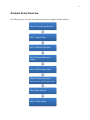
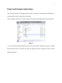
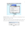
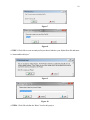
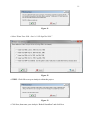
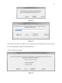
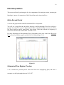
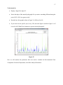
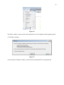
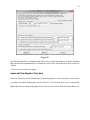
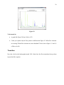
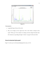
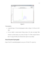
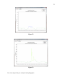
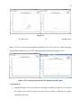
1
ESM 121
Water Science
and Management
Spring 2015
Exercise 6:
Flow Regime Analysis
Samuel Sandoval Solis, PhD
2
Contents
Objective ......................................................................................................................................... 3
Introduction ..................................................................................................................................... 4
Software Download and Data ......................................................................................................... 5
Analysis Setup Overview ................................................................................................................ 6
Project and Analysis Setup Steps .................................................................................................... 7
Data Interpretation ........................................................................................................................ 16
Entire Record Period ................................................................................................................. 16
Unimpaired Flow Regime: Pre-dam ......................................................................................... 16
Impaired Flow Regime: Post-dam ............................................................................................ 19
Transition .................................................................................................................................. 20
Annual unimpaired hydrograph ................................................................................................ 21
Annual impaired hydrograph .................................................................................................... 22
Comparing Monthly Median..................................................................................................... 24
Flow Duration Curves ............................................................................................................... 26
3
Objective
The aim of this tutorial is to gain a general understanding of how to use the Indicators for
Hydrologic Alteration (IHA) software to evaluate pre- and post-altered flow regimes. The flow
regime in the American River, prior and after the construction of the Folsom Dam, is used as
case study.
4
Introduction
The American River in runs 119 miles (192 km) from its headwaters in the Sierra Nevada to its
confluence with the Sacramento River, in Sacramento, CA. As part of the Central Valley
Project, the Folsom Dam was constructed in 1956 for the purposes of flood control,
hydroelectricity, and irrigation and municipal water supply. We will be using the IHA software
to analyze flow data below the Folsom Dam at the USGS Fair Oaks stream gage.
Figure 1: American River
5
Software Download and Data
• Unzip the tutorial zip file, which contains both the IHA software and the American River
USGS stream gage data from Fair Oaks, CA.
NOTE: The folder also contains files for another IHA tutorial included with the software that
will NOT be used in this tutorial. The tutorial you are doing now has been tailored for analysis of
a California relevant river system.
The IHA software is also available for download from The Nature Conservancy website.
http://www.conservationgateway.org/ConservationPractices/Freshwater/EnvironmentalFlows/M
ethodsandTools/IndicatorsofHydrologicAlteration/Pages/IHA-Software-Download.aspx
6
Analysis Setup Overview
The following is an overview of the basic steps taken to complete an IHA analysis.
Step 0: Set working directory
Step 1: Import data
Step 2: Name hydro data
Step 3: Create and name project
Step 4: Define water year
Step 5: Set up an analysis
•name, periods, statistics, graph titles
Step 6: Run analysis
Step 7: View results 7
Project and Analysis Setup Steps
This section will walk you through the IHA wizard, in which you will import the “FairOaks.txt”
stream gage data, then set up and run an analysis.
• In the unzipped “IHA71_En” folder, double-click on the IHA7 application to run the software.
Figure 2
• You will see the following window below. Click cancel. Before running the wizard, a working
directory needs to be set. If this is not done, the software will give remind you to do so before
starting an analysis.
8
Figure 3
•IMPORTANT STEP 0. Go to the Options menu and select “Set Working Directory.” Set your
working directory to the “IHA71_En” folder.
• STEP 1. Now you are ready to run the wizard. Under the IHA menu, select “Wizard.” The
window (Figure 4) will appear. Select OK for the next two windows to start the import process.
Figure 4
9
Figure 5
• Browse to the “FairOaks.txt” file provided with this tutorial. In the Import Dialog, select “Use
all data” and “cfs (cubic feet per second),” then click OK.
Figure 6
• STEP 2. Click OK to name your Hydro Data File “FairOaks.” While this tutorial only uses one
data set, multiple data sets can be added to your project.
10
Figure 7
Figure 8
• STEP 3. Click OK to create an analysis Project that is linked to your Hydro Data file and name
it “AmericanRiverProject.”
Figure 9
Figure 10
• STEP 4. Click OK to define the Water Year for this project.
11
Figure 11
• Select “Water Year 1994 = Oct. 1st 1993-Sept 30th 1994.”
Figure 12
• STEP 5. Click OK to set up an Analysis within this project.
Figure 13
• Click Next, then name your Analysis “BelowFolsomDam” and click Next.
12
Figure 14
Figure 15
This analysis will look at the impact of the construction of the Folsom Dam on the American
River by comparing pre- and post- impairment periods.
• Select “Compare two periods.”
Figure 16
13
Construction of the Folsom Dam was completed in 1956.
• Drag the slide control so that the time period on the left is “1905-1955” and click Next.
Figure 17
• Select “Non-Parametric Statistics” and click Next.
Figure 18
• Type in a title to display on the output tables and graphs, for example “American River below
Folsom”
14
Figure 19
• The next window reminds you that there are other custom setup options available. Continue
with the analysis by clicking Next.
Later in the tutorial, we will show you how to edit analysis parameters (Figure 28).
Figure 20
• The window below summarizes the parameters you have selected for this analysis. Click “Save
this Analysis.”
15
Figure 21
• STEP 6. Click OK to run the analysis.
Figure 22
You have now completed a basic analysis.
• STEP 7. Click OK to display the analysis output.
Figure 23
16
Data Interpretation
This section will walk you through a few key components of the analysis results, assessing the
hydrologic impacts of construction of the Folsom Dam on the American River.
Entire Record Period
• Activate the graph window titled Environmental Flow Components.
You will see a graph like the one below showing a daily hydrograph. Flow for each day is
grouped into one of five types of Environmental Flow Components (EFCs) (extreme low flows,
low flows, high flow pulses, small floods, large floods). Notice the difference in frequency of
flows before and after the Folsom Dam was built in 1956.
For more information on Environmental Flow Components, please refer to the book, Rivers for
Life by Postel and Richter (pg 49) and the IHA User Manual (pgs 13-15).
Figure 24
Unimpaired Flow Regime: Pre-dam
• Let’s examine the pre-dam period. Select the Zoom tool (magnifying glass) and draw a
rectangle over the hydrograph between 1912-1927.
17
To be turned in:

Display a figure like figure 25.

Notice the shape of the annual hydrographs. Do you notice something different during the
period 1923-1924? Any guesses why?

Describe how this graphic relates to Figure 2-4 of Rivers for life.

If you zoom in to an specific year, let say 1924, does this figure is similar to figure 1-4 of
rivers for life? What Flow elements are present in this hydrograph?
Figure 25
Now we will examine the parameters that were used to calculate the Environmental Flow
Components. From the Graph menu, select Edit Analysis Parameters.
18
Figure 26
The follow window warns you that certain parameters can’t be changed with the graphs opened.
• Click OK to continue.
Figure 27
• In the Analysis Properties window, activate the Environmental Flow Components tab.
19
Figure 28
The Environmental Flow Components tab allows you to modify parameters used in the algorithm
that calculates Environmental Flow Components, such as how small and large flood events are
defined.
• Click Cancel to return to the graph.
Impaired Flow Regime: Post-dam
Select the Zoom Out to Full Extent button (magnifying glass) to see the entire flow record. Draw
a rectangle around the hydrograph between 1966-1979. Note that the base flow is considerably
higher than in the pre-dam hydrographs. This is due to water releases from the Folsom Reservoir.
20
Figure 29
To be turned in:

A graph like Figure 29 from 1966 to 1979

Could you explain why the flow pattern is different that Figure 25. What flow elements
are missing? Which flow elements are more abundant? Take a look at Figure 1-5 and 4-2
of Rivers for life
Transition
Now take a look at the hydrograph around 1956. Notice how the flows transition from pre-dam
to post-dam flow regimes.
21
Figure 30
To be turned in:

A graph like Figure 30 from 1956 to 1964

Why are the changes in flow regime from 1956 to 1964. What is altering the flow
regime? What type of flow elements are missing and what ecological functions these
flow elements were providing (See figure 2-4, Box 2-1 at page 49 of Rivers for life)?
Annual unimpaired hydrograph
Figure 31 is close up view of the annual hydrograph for water year 1916.
22
Figure 31
To be turned in:

A graph like figure 31. Does this hydrograph is similar to Fugure 2-3 of Rivers for life?
Why?

Can you identify a seasonal pattern? During summer, fall, winter and spring? What
elements are presents during every seasons (See figure 2-3)? What ecological functions
(Box 2-1 at page 49 of Rivers for life) these flow regimes were providing?
Annual impaired hydrograph
Figures 32 and 33 are annual hydrographs for water years 1970 and 1972, respectively.
23
Figure 32
Figure 33
Now, lets compare the pre- and post- dam hydrographs.
24
Figure 34
Pre-Reservoir
Vs.
Post-Reservoir
Figure 35 (left) is close up for the annual hydrograph for the 1976 water year, which is during a
dry period that spanned two years. The right hydrograph is during the drought of 1923.
Figure 35: Post-dam dry period (left), Pre-dam dry period (right)
To be turned in:

A graph like figure 34. Can you discuss if this figure is similar to Figure 4-2 of rivers for
life? What is the reservoir doing to the flow? Do you think is affecting the aquatic
ecosystem of the river?
25
Comparing Monthly Median
Activate the graph window Monthly Flow for October and notice the median flows of pre- and
post- dam flows.
Figure 36
• Click on the IHA Graph Options button (leftmost) and select March.
Figure 37
26
To be turned in:

A graph like Figure 36. What is happening with the median flow of October in the
American River? Has it changed after the reservoir construction?
Flow Duration Curves
Activate the graph window for Flow Duration Curves.
Figure 38
27
Figure 39
• Activate the Project window. Right click on View Results and select View Tables.
Figure 40
• Select the sco worksheet to see the median pre- and post- dam flow values.
28
Figure 41
To be turned in:

Export the data highlighted in Figure 41 to excel and create a graphic like the following.
How the median flows has changed? Has it shifted? Has it been reduced?
29