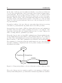
1
Heuristic Algorithms for
NP-Complete Problems
Thomas V. Christensen
Supervisor: Paul Fischer
Kongens Lyngby 2007
IMM-BSc-2007-12
Technical University of Denmark
Informatics and Mathematical Modelling
Building 321, DK-2800 Kongens Lyngby, Denmark
Phone +45 45253351, Fax +45 45882673
[email protected]
www.imm.dtu.dk
Summary
I have implemented a small framework of NP-complete problems in Java, where
it is possible to transform instances of one NP-Complete problem into instance
of another NP-Complete problem. The framework also consists of a few heuristic
algorithms, which makes it possible to find a heuristic solution for instances of
an NP-Complete problem.
Combining these two features it is possible to transform an instance of one NPComplete problem into another instance. This transformed instance may then
be solved by the available heuristic algorithm and the found heuristic solution
may then be detransformed to the original instance. Last but not least it is
possible to view this scheme through a nice user friendly GUI.
This report analyzes the design of the framework, the behavior of the heuristic
algorithms to transformed instances and how one may find the best transformation automatically to a given NP-Complete problem.
ii
Preface
This project was prepared at the institute of Informatics and Mathematical
Modelling, at the Technical University of Denmark from February through June
2007. It was one of the requirements for acquiring the B.Sc. degree in engineering.
Lyngby, June 2007
Thomas Vesterløkke Christensen
[email protected]
iv
Acknowledgements
I would like to thank my supervisor, Paul Fischer, who first of all introduced me
to this interesting field of computer science, but he has also advised and helped
me through the five months this project has lasted.
I would also like to thank my local pizza place for always giving me carbohydrates for my continuous respiration and sufficient fat and cholesterol, which
made any escape attempts from my desktop demand way more energy than I
can muster. An ideal solution for maintaining work, which can only be truly
appreciated in the eyes of an engineer.
vi
Contents
Summary
Preface
i
iii
Acknowledgements
v
1 Introduction
1
2 Motivation
5
3 Scope of Project
9
4 The NP-Complete Problems
11
4.1
The necessary theory . . . . . . . . . . . . . . . . . . . . . . . . .
11
4.2
Theory in use . . . . . . . . . . . . . . . . . . . . . . . . . . . . .
13
5 Extending the framework
15
viii
CONTENTS
5.1
Design of Problems . . . . . . . . . . . . . . . . . . . . . . . . . .
16
5.2
Design of Heuristic Algorithms . . . . . . . . . . . . . . . . . . .
17
5.3
Design of Transformations . . . . . . . . . . . . . . . . . . . . . .
18
5.4
Design of Detransformations . . . . . . . . . . . . . . . . . . . . .
21
6 Automatic solving
25
6.1
Constructing the graph . . . . . . . . . . . . . . . . . . . . . . .
25
6.2
Finding the shortest route . . . . . . . . . . . . . . . . . . . . . .
27
6.3
Heuristic Algorithms . . . . . . . . . . . . . . . . . . . . . . . . .
31
6.4
Multiple transformations . . . . . . . . . . . . . . . . . . . . . . .
32
6.5
Implemented solutions . . . . . . . . . . . . . . . . . . . . . . . .
32
7 Design of Graphical User Interface
35
7.1
Creating problems . . . . . . . . . . . . . . . . . . . . . . . . . .
37
7.2
Transforming, solving and detransforming instances
. . . . . . .
41
7.3
Final Design
. . . . . . . . . . . . . . . . . . . . . . . . . . . . .
42
7.4
More sophisticated features . . . . . . . . . . . . . . . . . . . . .
43
8 Code overview
45
9 Strategy for data gathering
47
9.1
Random Satisfiability input . . . . . . . . . . . . . . . . . . . . .
10 Results
10.1 Theoretical results from Satisfiability . . . . . . . . . . . . . . . .
48
51
51
CONTENTS
ix
10.2 Testing setup . . . . . . . . . . . . . . . . . . . . . . . . . . . . .
53
10.3 The Zeus algorithm . . . . . . . . . . . . . . . . . . . . . . . . . .
53
10.4 The Hera algorithm . . . . . . . . . . . . . . . . . . . . . . . . .
61
10.5 The Poseidon algorithm . . . . . . . . . . . . . . . . . . . . . . .
62
10.6 What was not completed . . . . . . . . . . . . . . . . . . . . . . .
63
11 Conclusion
65
11.1 Where to go from here . . . . . . . . . . . . . . . . . . . . . . . .
A Creating Random Satisfiability Instances
67
69
A.1 First suggested algorithm . . . . . . . . . . . . . . . . . . . . . .
69
A.2 Second suggested algorithm . . . . . . . . . . . . . . . . . . . . .
70
B Heuristic Algorithms
73
B.1 Zeus . . . . . . . . . . . . . . . . . . . . . . . . . . . . . . . . . .
73
B.2 Hera . . . . . . . . . . . . . . . . . . . . . . . . . . . . . . . . . .
75
B.3 Poseidon . . . . . . . . . . . . . . . . . . . . . . . . . . . . . . . .
77
C Data Tables
79
D User Manual to Program
83
D.1 Creating Instances . . . . . . . . . . . . . . . . . . . . . . . . . .
83
D.2 Transforming Instances
. . . . . . . . . . . . . . . . . . . . . . .
88
D.3 Solving Instances . . . . . . . . . . . . . . . . . . . . . . . . . . .
88
D.4 Finding Best Solution . . . . . . . . . . . . . . . . . . . . . . . .
89
x
CONTENTS
D.5 Detransforming Instances . . . . . . . . . . . . . . . . . . . . . .
E API Manual
89
91
E.1 New Problems . . . . . . . . . . . . . . . . . . . . . . . . . . . .
91
E.2 New Transformations . . . . . . . . . . . . . . . . . . . . . . . . .
92
E.3 New Heuristic Algorithms . . . . . . . . . . . . . . . . . . . . . .
93
E.4 Updating the Framework . . . . . . . . . . . . . . . . . . . . . .
93
E.5 New GUI Problems . . . . . . . . . . . . . . . . . . . . . . . . . .
94
E.6 GUI Transformations . . . . . . . . . . . . . . . . . . . . . . . . .
95
E.7 GUI Update . . . . . . . . . . . . . . . . . . . . . . . . . . . . . .
95
Chapter
1
Introduction
In Computer Science there is a complexity class of problems known as NPComplete (NPC), because they contain complete information about all problems
in the complexity class NP. The way of proving a problem is NPC is to make
a polynomial(fast) transformation from a known NPC problem to the problem
considered and showing that this transformation yields the same solutions for
both problems. The relationship between NPC, NP and the class of problems,
where a solution can be found in polynomial time, P, can be seen in Figure 1.1.
Figure 1.1: Relation between complexity classes
2
Introduction
At the time of this project it is unknown whether or not these problems can
be solved in polynomial time, but it is strongly believed that it requires superpolynomial time. However if it would be possible to solve one NPC problem
in polynomial time then all NPC and NP problems can be solved in polynomial time. This is because of the polynomial transformations between the NPC
problems. On the other hand if it is possible to show that one of the problems
cannot be solved in polynomial time, then none of the problems can be solved
in polynomial time.
Presently no valid proof for any of the two cases exists, there is however a strong
belief that no polynomial time algorithm exist for the NPC problems.
In general there is two kinds of NPC problems called decision and optimization
problems, where the first consists of finding if it is true or not and the other
represents a problem where an optimal solution needs to be found. This project
will be working with the optimization problems.
The method used so far for solving NPC optimization problems is making heuristic algorithms that gives approximate or suboptimal solutions to the considered
problem. These algorithms can as well use the transformations to give approximate solutions to other NPC optimization problems like shown in Figure 1.2.
The argument for doing this is that the transformation is very often easier and
less time-consuming to implement and develop than creating a new heuristic
algorithm from scratch.
Prob1
1. Transform 3. Detransform
2. Solve
Prob2
Algorithm
Figure 1.2: Using an algorithm to solve more than just one kind of NPC problem.
The goal of this project is to make it possible to solve instances of NPC problems by transforming them to problems where heuristic algorithms are available.
3
Furthermore the behavior of the heuristic algorithms will be analyzed when the
transformations are used. The project should also allow the user to use a graphical user interface, such that the transformed problems and their approximate
solutions can be seen by the user.
4
Introduction
Chapter
2
Motivation
The motivation for doing this project is first of all to see if it is beneficial to
reuse heuristic algorithms by using the available transformations. Should it
prove not to be feasible, then it can be used to find transformations that create
bottlenecks.
Another benefit of the transformation is that for a single NPC problem one can
get access to a variety of different algorithms.
With the graphical user interface this project will be excellent for teaching
purposes, such that one can get an intuitive understanding of how instances are
transformed. This feature will also make it an excellent tool, when trying to
create and verify new transformations.
Another interesting aspect, which can be seen in Figure 2.1a, is that the transformations allow one to compare two different algorithms from two completely
different problems. With this opportunity one might be able to investigate the
characteristics of good heuristic algorithms.
However what if a heuristic algorithm gives great results for the problem it
was created for, see Figure 2.1b, does this necessarily mean that it will also
give great results when detransformed to other problems? All we know is that
if a transformed instance can be solved then the solution will also solve the
6
Motivation
Prob1
Prob2
Algorithm1
Prob3
Algorithm2
(a)
Prob1
? % of opt. solution for Prob1
Prob2
Algorithm
80 % of opt. solution for Prob2
(b)
O riginalProblem
Transform edProblem
detransform :M ethod
detransform ()
(c)
Figure 2.1: Diagram of (a) how to use and compare different algorithms from
different NPC problems detransformation (b), compare heuristic solutions to
see if the it is equally good for the transformed and the original instance (c) and
detransforming of an algorithm to another NPC problem.
7
original instance, but when the instance cannot be solved we instead find a
good estimate. Is this estimate still good when it is detransformed?
It is time-consuming to develop new heuristic algorithms, but what if one manually detransformed the entire heuristic algorithm like shown in Figure 2.1c,
then the transformations of instances to other NPC problems would no longer
be done and all we had to do was run the algorithm.
These are all just a handful of interesting aspects, which this project can help
find answers for.
8
Motivation
Chapter
3
Scope of Project
It is the aim of the project to implement a decent number of transformations to
different kinds of NPC problems and develop various kinds of algorithms for a
subset of these problems. The algorithms I implement will be my own, because
I figure it might be a good idea to start from scratch, this however does not
guaranty that the algorithms I end up with are original, and I will not spend
any time investigating whether or not that be the case.
In the project I emphasize the following:
• This is not just a proof of concept. It is meant to be optimized for practical
use,
• it should be easy for third party to extend the framework with new problems and transformations that uses the existing heuristic algorithms,
• it should be easy for third party to extend the framework with new heuristic algorithms,
• the framework should be able to find the best suited transformations automatically,
• and for the problems implemented the transformed problem input/output
should be viewable in nice graphical user interface.
10
Scope of Project
It should be mentioned that I do not intend the developed software to be Open
Source Software. This means that certain measures need to be taken, if it should
be easy for the third party to extend it without actually knowing the source code.
In this sense I see it as a benefit that the source code is not Open Source, since
less information is needed. However I feel that making this choice, requires me
to make a manual describing how the framework should be extended.
Furthermore to optimize the framework I chose not to use proper encapsulation
of data in order to avoid the overhead of get- and set-methods. This is however
only carried out in the data structures, because they are the ones, which will be
used the most.
This project does not in any way aim to prove or disprove the N P = P problem.
Chapter
4
The NP-Complete Problems
This section shortly describes precisely what a NP-Complete problem is and the
process of proving NP-Completeness for a problem. This section will not give
a complete explanation regarding the theory of complexity classes or why the
process is a valid proof, but instead focus on how the theory can be used in this
project and what obstacles one should expect just by looking at the theory.
4.1
The necessary theory
There is one complexity class of problems called NP, which stands for nondeterministic polynomial time. Given a solution for such a problem, one can in
polynomial time verify that it is indeed a solution for the problem.
However there is a set of problems in NP, which are proven to be more or at least
as difficult to solve as all other problems in NP. These problems are called NPComplete(NPC), because they are said to contain complete information about
all problems in NP, the relationship between NPC, NP and P can also be seen in
Figure 1.1. The immediate result of this is that if one can solve a NPC problem
efficient then all problems in NP can be solved efficient.
The first problem to be proven NP-Complete was the Satisfiability problem (for
12
The NP-Complete Problems
a proof see [4]). In general there are two types of NPC problems called decision
problems and optimization problems. A decision problem is a NPC problem
where the answer is yes or no, while the optimization problem is the best solution
for a given problem. So if I have a instance of the Satisfiability problem and I
ask if it can satisfy e.g three clauses then it is a decision problem, however if
I instead want to know the assignment that satisfies most clauses then it is a
optimization problem. This project will be dealing with optimization problems.
Now given one NPC problem, P1 , one can prove a problem, P2 , is NP-Complete
if it is harder or just as hard as P1 1 . The P2 is proven NP-Complete by:
1. Showing it is in NP,
2. and constructing a transformation, that transforms instances, I1 , of P1 to
instances, I2 , of P2 .
• This transformation must have polynomial running time
• If there is a solution for I2 then there also is a solution for I1 .
• If there is a solution for I1 then there also is a solution for I2 .
• The transformation should show that P2 is harder or just as hard as
P1 , because P1 can be solved by solving P2 .
It is easy to prove the problem is in NP, however constructing the transformation
can require a great amount of creativity. To show the transformation makes P2
harder than P1 , as a rule of thumb one just have to find an instance of P2 , which
cannot be detransformed to P1 . This means all of the instances of P1 will be
transformed into special cases of P2 . Therefore P2 is harder than P1 , because
all instances of P1 is just a subset of all instances of P2 . This rule of thumb does
not apply when the problems are exactly the same or very close related, which
is the case with Independent set, Clique and Vertex Cover.
If the transformation yields special cases as described above, then one might
confuse a transformation with a problem reduction and maybe it is. But one
should remember that all NPC problems are equally hard and this does not
contradict with transformations producing special cases, because the cost of
special cases are padding. In other words the transformations make the problem
size increase, which is important to note, since it pose a great problem for this
project.
1 The problem can off course not be harder since a NP-Complete problem is defined by
being harder than all other problems.
4.2 Theory in use
4.2
13
Theory in use
The general goal in computer science is to find the best possible solution to all
problems as fast as possible, which in most cases means in polynomial time.
The idea behind this project is to reuse the polynomial transformations that
were created just to proof NP-Completeness.
Let us say we have a transformation going from a problem, P1 , to another
problem, P2 , and for this specific problem we have a good heuristic, polynomial
time algorithm. Then it it possible to transform any instance, I1 , of P1 to an
instance, I2 , of P2 , solve I2 with the algorithm and detransform the solution back
for I1 . Note that if this project had worked with decision problems instead of
optimization problems then the detransformation process would be unnecessary
since the answer would remain the same after a detransformation.
The process just described can all be done in polynomial time and by the definition a satisfying solution for I2 can be detransformed into a satisfying solution
for I1 . If one cannot find a solution for I2 then it is not possible to find a solution
for I1 either. This also means that if one can find a polynomial time algorithm
which finds the optimal solution for one NPC problem then all NPC problems
can be solved in polynomial time.
However no such algorithm are currently known, so [6] describes three ways of
solving a NPC problem:
1. using exhaustive search to find the optimal solution for small problems
which gives a exponential running time,
2. to recognize special cases of a NPC problem, which can be solved optimally
in polynomial running time,
3. or to use an algorithm with polynomial running time which finds a nearoptimal solution.
This project will work with the last two types of algorithms mostly dealing with
the last type, which is also called heuristic algorithms.
Now if one gets a good solution for I2 using a heuristic algorithm, then the
definition does not guaranty that the detransformed solution is just as good for
I1 . But of course if the solution was optimal, then it will also be optimal when
detransformed.
14
The NP-Complete Problems
Furthermore it is interesting to see if the special cases, that the transformations
produce, have a certain structure, which makes them easier to solve. If it is
the case that a transformation always produce a certain kind of instances of a
problem, that are easy to find the optimal solution for, then one has a polynomial
time algorithm which solves a NPC problem optimally.
One of the goals of this project is to make it easy to extend the framework with
new NPC problems. As explained above to show a problem, P , is NP-Complete
one has to show it is in NP and construct a valid transformation, T 1, from a
known NPC problem to P . However the reason for extending the framework
with new problems is to solve these problems with the existing algorithms, but
this is not possible with the T 1, since it cannot transform instances of P to any
problems in the framework, which has an algorithm. So furthermore one has
to create another transformation, T 2, going from P to one of the existing NPC
problems, preferably one which has access to many good or fast algorithms.
This scheme can be seen in Figure 4.1.
Known NPC Problem
Algorithm
T1: proves P is NPC. T2: makes algorithm available.
P
Figure 4.1: What transformation to make when extending with new NPC problems.
Chapter
5
Extending the framework
This section analyzes the design of different solutions for making the framework
easy to extend for third party.
Basically there are only three kinds of extensions the framework needs to support
– new problems, new transformations and new heuristic algorithms.
Thus I define three properties of the framework, that the final design should be
able to handle in a proper way.
Property 1 An instance can be transformed to different problems and have
multiple heuristic algorithms.
Property 2 A solution for a transformed instance can be detransformed to a
solution for the original instance.
Property 3 A problem can be transformed to the same problem with different
transformations.
Notice that these properties should not only be handled by the design in general,
but they should also be given to the user that wishes to extend the framework.
16
Extending the framework
Also note that the third property is not necessarily needed, since most problems
only have one transformation. This is mainly because it only takes one transformation to prove a problem is NP-Complete, but if one locates a bottleneck
transformation, then it should be possible to add a new and better transformation without removing the existing one.
5.1
Design of Problems
The most obvious choice for implementing a problem is by a class of its own.
The methods of this class could then do transformations, detransformations and
heuristic algorithms.
So if the framework is to be extended with a new problem, it should just inherit
an abstract class called NPCProblem , see Figure 5.1. Then all the new class
should contain is the input for the given problem, so the design would look
something like this:
1
2
3
4
5
6
7
8
9
class P extends NPCProble m {
// data fields
...
// t r a n s f o r m a t i o n methods
...
// d e t r a n s f o r m a t i o n methods
...
// heuristic algorithm methods
... }
N PC Problem
P1
P2
P3
Figure 5.1: Class diagram of NPC problems inheriting NPCProblem.
Using this representation the user still have the opportunity of extending existing problems simply by inheriting those problems and supplying new methods(transformations, algorithms, etc.).
5.2 Design of Heuristic Algorithms
17
Overall this seems as the only right way to represent problems in an ObjectOriented Programming Language.
5.2
Design of Heuristic Algorithms
Given that problems are represented by classes the heuristic algorithms are more
or less bound to be methods of the class, if it should have easy access to the
data for the given problem. Thus the algorithms can be implemented as:
1
2
3
Solution algo1 () {...}
Solution algo2 () {...}
...
This design also makes it possible to supply new algorithms for existing problems
without overriding the old algorithms.
However using this design one can chose to simply return the solution, which
would work just fine, but it may be a good idea to store the solution in the
instance of the given problem. Doing this would make it necessary to store
a solution for each of the algorithms, which would require a great amount of
memory – possibly more memory than the input for the problem.
I chose not to save the solution, because the motivation for saving them is not to
compute the solution again in case the user should think of calling the algorithm
every time he1 wanted the solution.
Just to underline that it is a bad idea to store the solution, consider the case
when an instance can get a solution from a transformed instance. This means
that the instance should be able to store a solution for each algorithm available
in the transformed instance and so on. In the case a solution was found in
a transformed instance, then the solution would also had to be stored in the
transformed instance. In other words it is a waste of space to store the solution
at this point.
1 Throughout this report I will refer to third party as he or him. This should not be seen
as an act of prejudice but rather a sad statistical observation.
18
5.3
Extending the framework
Design of Transformations
As with the algorithms the transformations are bound to be methods in the
NPCProblem class or its subclasses and it is also required that this method
should somehow return another NPCProblem. However the best structure of this
method is anything but easy to find. Therefore I list in the following a number
of suggested solutions, which all have their advantages and disadvantages.
First suggestion The first way it could be structured is like:
1
NPCProble m transform ()
It is very general, which means that it can be put in the abstract class NPCProblem,
such that all classes inheriting NPCProblem will be bound to implement the
transformation like shown in Figure 5.2a.
However not all NPC problems have a transformation, which makes it a bad
idea furthermore only one transformation is available and the user have no idea
what kind of problem the transformation creates. Now if the user were to supply
a new transformation for an existing NPC problem he would have to override
the existing transformation.
In other words this seems as a very poor choice for implementing transformations
since none of the desired properties for the framewrok are achieved.
Second suggestion Now consider another way in which the transformation
can be structured:
1
2
3
4
5
6
NPCProble m transform ( Class <? extends NPCProblem > c ) {
if ( c . equals ( P1 ) )
// return transfor me d prob P1
else if ( c . equals ( P2 ) )
// return transfor me d prob P2
... }
Using this structure one can still place the method in the abstract class NPCProblem
as shown in Figure 5.2b and it supports the first property by supplying transformations for different problems.
If new transformations are to be added the method would have to be overwritten,
however the existing transformations could still be used:
5.3 Design of Transformations
19
N PC Problem
N PC Problem
transform ():N PC Problem
transform (c :C lass<?>):N PC Problem
P1
P2
P1
P2
(a)
(b)
N PC Problem
N PC Problem
transform (t:int):N PC Problem
P1
P1
P2
(c)
P2
transform P2_1():P2
transform P2_2():P2
transform P1():P1
(d)
Figure 5.2: UML diagram of (a) the first suggested solution (b), the second
suggested solution (c), the third suggested solution (d) and the fourth suggested
solution.
20
1
2
3
4
5
6
7
8
Extending the framework
// overridde n method
NPCProble m transform ( Class <? extends NPCProblem > c ) {
super ( c ) ;
if ( c . equals ( newP1 ) )
// return transfor me d prob newP1
else if ( c . equals ( newP2 ) )
// return transfor me d prob newP2
... }
But this design does not allow multiple transformations to the same problem –
second property of the framework is unavailable. Beside that I find that all the
if-statements look terrible, but from the perspective of the user it makes it easy
to just have one transformation-method.
Third suggestion By modifying the previous design one could use the one
shown in Figure 5.2c and below:
1
2
3
4
5
6
7
NPCProble m transform ( int t ) {
switch ( t ) {
case T R A N S F O R M 1 _ T O _ P 1 : // return P1 using first t r a n s f o r m a t i o n
case T R A N S F O R M 2 _ T O _ P 1 : // return P1 using second t r a n s f o r m a t i o n
case T R A N S F O R M 1 _ T O _ P 2 : // return P2 using first t r a n s f o r m a t i o n
...}
}
This design allows transformations to different problems and multiple transformations to the same problems and it can be placed in the abstract class
NPCProblem. Furthermore it still allows the user to extend existing problems
with new transformations without overriding the existing transformations in the
same way as in the lat suggestion. The downside of this design is that the user
has to know the values of the existing constants(TRANSFORM1 TO P1, ...) when
adding his own transformation. Another undesired thing about this design is
like before that one do not know for sure what type of NPCProblem the method
returns.
Fourth suggestion My last and final suggestion for designing the transformations can be seen in Figure 5.2d and below:
1
2
SAT t r a n s f o r m T o S A T 1 () { .. }
SAT t r a n s f o r m T o S A T 2 () { .. }
This design gives every transformation its own unique method, which makes
it easy to extend, because when one inherits the class a new transformation
5.4 Design of Detransformations
21
method can just be added. Another benefit is that one actually knows what type
of NPC problem is returned and like the previous suggestion it achieves all three
properties of the framework, which explains why this is how the transformations
have been implemented.
However not all is well, the above suggestions all suffer from the same problem,
which seems to be difficult to solve unless the source code is open. Consider the
case in Figure 5.3, where the class, SAT, representing the Satisfiability problem
is extended by a third party with new algorithms and transformations, which
is called SAT2. The problem arises when the other NPC problems have transformation to the SAT and not SAT2 class. This can be solved my extending all
the other problems and make them make transformation to SAT2 instead or by
making a constructor for SAT2, which takes a SAT object as argument.
N PC Problem
P1
SAT
transform SAT():SAT
SAT2
transform P2():P1
Figure 5.3: Problematic situation for third party to extend a existing
NPCProblem class.
But still none of those two solutions are satisfying compared to how easy it
would be if the source code was available. The extensions can nonetheless be
done with this design.
5.4
Design of Detransformations
I find that the greatest problem in detransforming a solution from a transformed
instance is that one cannot distinguish between a transformed and a user-defined
instance. Furthermore if one could, then it would still be necessary to know what
NPC problem to detransform the solution to.
22
Extending the framework
Detransforming a solution is more or less bound to be a function in the NPCProblem
classes. Note now that the previous choice of not storing the solution found by
the algorithms, means that the solution needs to be a parameter for the detransformation method. This actually solves two problems in the detransformation
process. First of all the solution is provided as a parameter by the user, so
it does not need to bother about whether or not a transformed instance has
found a solution. Secondly the method no longer has to decide what solution to
detransform if there is more than one algorithm for a NPCProblem. The same
goes if there are solutions from two different transformed instances.
The downside is that the user can now give a parameter which has never been
a solution for the transformed instance.
There are two obvious approaches, which one can use for the detransformation:
1. The method can be called from the transformed instance and send the
detransformed solution to its original instance as in Figure 5.4a,
2. or it can be called from the original instance and it will detransform the
solution from its transformed instance like in Figure 5.4b.
In both cases the detransformed solution needs to be returned, so both approaches yields the same result since nothing is stored, which is a consequence
of the choice described above.
With the first approach one would have to store a reference to the original
instance it was transformed from, since it is necessary to know what kind of
NPCProblem to detransform back to. When detransforming one needs to know
a lot of details of the original instance, which means that every NPCProblem
would need a lot of get-Methods in order to make the detransformation. In
the case where an instance can use more than one transformation to the same
NPCProblem , the transformed instance would have to somehow know, which
of the transformations that were used, which could be done with some sort of
constant variable.
Using the second approach most of the above problems are gone except for
the problem of deciding what detransformation method to use if the problem
contains more than one transformation. This is a problem since a solution
contains little information on what transformed instance it came from. Using
this solution the transformation and detransformation methods will be placed
in the same class, which seems to be beneficial.
It might seem as an obvious choice, however if I had chosen that the solutions
5.4 Design of Detransformations
23
Transform edProblem
O riginalProblem
detransform ()
(a)
O riginalProblem
Transform edProblem
detransform ()
(b)
O riginalProblem
Transform edProblem
detransform :M ethod
detransform ()
(c)
Figure 5.4: UML diagram of (a) first suggested solution for detransformation
(b), second suggested solution for detransformation (c) and the third suggested
solution for detransformation.
24
Extending the framework
from the algorithms were stored in the problems, then it might not had been so
obvious, because then a lot of work could possibly be removed from the user by
choosing the first suggested solution.
There is actually also a third option where the actual detransformation method
is placed at the original instance but called by the transformed instance, which
is shown in Figure 5.4c. This can be done elegantly by using Javas reflection
library to give the Method object for detransforming to the transformed instance,
which will then know how to detransform a solution. I chose however to stick
with the second solution because in order to use the last solution the method
has to be public(or protected if the classes are in the same package), which is
what has to be done in the second solution.
Now from the previous choices made the detranformation is bound to take a
solution as parameter and return a detransformed solution, which gives the
following design:
1
d e T r a n s S o l u t i o n d e t r a n s f o r m 3 S A T ( Solution s ) { .. }
In order to support multiple detransformations for the same problem the same
scheme can be used as for the transformation methods:
1
2
d e T r a n s S o l u t i o n d e t r a n s f o r m 3 S A T 1 ( Solution s ) { .. }
d e T r a n s S o l u t i o n d e t r a n s f o r m 3 S A T 2 ( Solution s ) { .. }
The final design for the framework now handles all the wanted properties and
can be extended by a third-party. It does not waste memory on solutions that
are never made and it gives a lot of control to the user. This on the other hand
also makes the design vulnerable to human errors.
Chapter
6
Automatic solving
Solving a problem automatically with the best suited transformations and heuristic algorithm can be done in a number of different ways. This chapter describes
the problems when solving problems automatically.
It is obvious that this problem is nothing else but to find the shortest route
between two problems in terms of transformations. Because problems are connected together with the transformations, one can construct a directed graph
with the problems as vertices and the transformations as directed edges as shown
in Figure 6.1. Now in order to find the shortest route between two problems
one just have to implement Bread-First-Search or the Dijkstra algorithm. This
all seems straight ahead however there are some issues one should consider.
6.1
Constructing the graph
When constructing the graph, it is crucial not only for it to contain all NPC
problems and transformations but also information on what method to call in
order to use the given transformation or algorithm.
The simplest way of doing this is to manually type in all transformations and
algorithms and their respective methods. However this would not only be time
26
Automatic solving
Satisfiability
3-Satisfiability
N/A
3-Dimensional Matching
Partition
Subset Sum
BinPacking
Hamilton Path
Hamilton Cycle
Traveling Salesman
Vertex Cover
Clique
Independent Set
KnapSack
Figure 6.1: Transformation graph showing all NPC problems and transformations.
6.2 Finding the shortest route
27
consuming but also very inflexible, because one might make a long switch-case
statement, which looks at what transformation should be called and then calls
it.
All these problems can nonetheless be solved very elegantly using Javas reflection
library, which allows one to see a complete list of all methods within a given
class. This functionality can be used to automatically retrieve all transformation
methods from a class in order to create the needed graph. It does however not
contain information on the subclasses of a class, which makes it necessary to
give all the subclasses of NPCProblem to the program.
Also if one has the name of a method, then Java allows one to call the method
on an object, just by passing a string containing the name of the method. This
solves all the problems from above. The downside in using this is that if the
program should automatically recognize transformation and algorithm methods,
then they must have a certain structure or name. So if a third party should
extend the framework with new transformations then it is something he should
be aware of.
To be specific I have chosen that all transformation methods must start with
the keyword ”transformTo“ and ended with some suffix. The corresponding
detransformation method must start with the keyword ”detransform“ and be
ended with the same suffix as with their transformation method. The methods
for the algorithms must start with the keyword ”algo“. Below is shown an
example:
1
2
3
4
5
6
public
public
public
public
public
public
<V > VertexCover <V > t r a n s f o r m T o V C () {...}
T h r e e D i m e n s i o n a l M a t c h i n g t r a n s f o r m T o 3 D M () {...}
boolean [] d e t r a n s f o r m V C ( boolean [] vcsolution ) {...}
boolean [] d e t r a n s f o r m 3 D M ( boolean [] tdmsoluti o n ) {...}
boolean [] a l g o S o m e N a m e () {...}
boolean [] a l g o S o m e O t h e r N a m e () {...}
Another issue using the reflection libraries is that the compiler cannot make
typechecking to see if the correct parameters are used or returned, which is like
playing with fire.
6.2
Finding the shortest route
Finding the shortest way to solve a instance is entirely easy to solve, but I see
three different ways this can be done:
28
Automatic solving
• Every transformation is given the same weight,
• or one looks at the asymptotic running time for each transformation,
• or one uses a statistical value from previous runs of a transformation.
6.2.1
Shortest route using Breadth-First-Search
The first solution is very simple to implement, since it is basically just breadthfirst-search. The benefit from using this method is that it is easy to implement,
it is flexible to new transformations, and it is a somewhat good estimate for the
shortest transformation path. It however does not take into account that the
transformations have different running time and a different degree of padding,
so in this sense it is a bit too naive.
6.2.2
Shortest route using Asymptotic running time
The second solution looks from a theoretical point of view much better and
should be easy to implement, however it introduces some difficulties.
Normally we write the asymptotic running time using the O-notation, which
shows the most significant term as a function of the input size, this means that
if one uses two transformations for a given instance of a problem, where the first
have the running time O(n3 ) and the second O(n2 ), then the running time of
taking both transformations would yield a running time of O(n3 + n2 ) = O(n3 ).
This is a very simple scheme which can easily be implemented by letting the
weight of a path be determined by the largest exponent from the asymptotic
running times of all the transformations in a path.
This solution is clearly a bit better than the first, however it assumes that there
is no padding when doing a transformation and this is rarely the case. Now
consider the same two transformations from before, where the first transformation is given an input of size n and after the first transformation the size of the
transformed input has increased to a size of n2 as a result of padding. Now the
running time of first transformation is still O(n3 ), however the running time
of the second transformation is now O((n2 )2 ) = O(n4 ), which yields a total
running time for the two transformations to O(n3 + n4 ) = O(n4 ).
Obviously this is a more descriptive solution, however there are a couple of
problems.
6.2 Finding the shortest route
29
The first problem is that the above strategy assumes that the input size is
determined by one parameter, which is rarely the case. For instance a graph
transformation may take O(V 2 + E), where there is not only two different parameters but also two different exponents, which makes the scheme above a bit
more tricky to implement.
Another problem is that one needs to feed the transformation with some kind of
function, such that it is able to calculate how much the input size will increase.
Last problem is when the Dijkstra algorithm is running, the instance to be
transformed has not yet been created which means that Dijkstra does not know
the input size of the instance and can therefore not do the calculations.
One could however create the instance before running Dijkstra, but if one is
creating multiple instances of the same problems, then Dijkstra would have
to run each time to find the shortest route. This may however be satisfying
if the instances are very large and time can be saved by finding the shortest
transformation path each time.
6.2.3
Shortest route using statistical data
Using the asymptotic running time for finding the shortest route seems to be a
very clever choice from a theoretical point of view, but it has its limits. First of
all the O-notation removes all constants and minor terms, which may be very
significant even for medium sized input, however this is not really interesting
since this project aims to solve large problems efficiently.
What is interesting is that the running time of computers is highly dependent
on, how much time is has to wait for retrieving data from main memory. To
speed up this process most computers stores recently used data close to the
CPU in Cache Memory, which takes less time to access. The great problem is
that the Cache Memory has different sizes and operates differently on different
computers.
So bottom line is that using the asymptotic running time may not be a good
idea, since it does not take into account how the computer operates. On the
other hand it is way beyond this project to try and predict how an instance is
transformed optimally on a specific computer. It would however seem as a good
idea to find the shortest route based on empirical data for the used computer.
Doing this introduces a number of issues. The first is what data to store and
how to use is for future runs, another issue is that the data should be updated
30
Automatic solving
every time the transformation is used, such that it is up-to-date. It is obvious
that data needs to be stored for each transformation if it is to be changed.
Clearly it would be a bad idea to store data from each time the transformation
was used, since the data then would be grow tremendously in no time. Another
problem of having all that data is that it has to be processed every time Dijkstra
is used. The way to solve this is to some how find an average of the data gathered
and then to store this average. One could choose to simply take the average
time of all the transformation runs, however since the time depends very much
on the input size, n,this solution would be a bad idea. Instead the average time
should be weighted with respect to the input size. Since all the transformations
run in polynomial time one can assume that the time depends on the input size
by some polynomial:
time = nk ⇔ k =
log time
log n
So for each run of the transformation one could calculate the exponent k take
the average and use this as the actual asymptotic exponent like described above.
The drawback of using this simple method, is like explained above that not all
transformations depends on just one input size e.g most graph transformations
depends both on the number of edges and vertices. If the function depends on
more than one value then it is likely that the values are not equally significant
and that they should be weighted. Another problem is that not all transformations have a running time which can be described by a polynomial e.g n lg n.
Whenever a transformation has been used the stored value should be updated,
however if the old value is based on the results of hundreds of transformation
runs, then it should not be affected too much by a single outlier. In other words
the stored data should include information on how many transformation runs,
m, the average value, vold , is based on. So when a new piece of data, d, is
collected the old average value should be updated like this to include the new
data:
vold m + d
m+1
= mold + 1
vnew =
mnew
Compared to the simple way of using the asymptotic running time, this statisti-
6.3 Heuristic Algorithms
31
cal data takes padding into account, but instead of taking a simple average one
could instead try and find a polynomial with highest degree d, which fits the
data as well as possible and then use it along with data on a specific problem.
This would only require that all the coefficients for the polynomial is saved, however it is very tricky to update them. It is beyond the scope of this project to
investigate on how to do it, but if one have knowledge of how many former runs
the polynomial is based on and one assumes that these samples are uniformly
distributed over an interval for the polynomial, then it is possible to calculate
the new updated coefficients.
As previously mentioned the transformations produce instances, which have a
certain structure and some of these instances are transformed further on which
produce another kind of instances with a special structure. This means that
the statistical data gathered may very well be based on a certain kind of input,
which is a problem if this kind of input has been used for a period of time and
then a new kind of data is using the transformation. The new kind of data may
now be choosing a bad transformation for this kind of input, which is a problem
when using the empirical data the way it is suggested above.
Furthermore if a transformation has initially proven to be bad for a number
of instances then it will get a expensive weight which makes it unlikely that
Dijkstra will choose to use this transformation ever again. This may prove to
be wrong for other types of instances, than the ones the empirical data was
based upon. This suggests that it would be a good idea to introduce some sort
of randomness in Dijkstras algorithm when using empirical data.
6.3
Heuristic Algorithms
So far it has been discussed how to find the route from one problem to another
which takes as little times as possible, however it also takes time to find the
heuristic solution, so it may be desired to let the algorithms be part of the
calculations when finding the cheapest route. On the other hand the main
purpose is usually to find the optimal solution for a problem, which makes it
naive to think a fast algorithm can create as good results as a slower algorithm.
If the algorithms should be included in the calculations then I see the same three
ways of doing it:
• One could give all algorithms the same weight,
• or one could use their asymptotic running time and optionally take padding
32
Automatic solving
into account in the same way as with the transformations
• or use empirical data for the algorithms.
All three solutions can more or less be done in the same way as with the transformations.
6.4
Multiple transformations
When having more than one transformation, which transforms from problem,
P1 , to another problem, P2 , as shown in Figure 6.2a, then the graph used with
Dijkstra should be able to contain parallel edges. Parallel edges is not a problem
if the graph data structure uses adjacency list, however when using adjacency
matrix only one edge can be store between two vertices. This can be solved by
letting the remaining edges go to its own new intermediate vertex, which has
an edge to the end vertex with no weight. This solution can be seen in Figure
6.2b.
P1
P1
T2
T1
T1
T2
T3
T3
Dummy1
T4
Dummy2
Dummy3
T4
0
P2
(a)
0
0
P2
(b)
Figure 6.2: Example of (a) multiple transformations between two NPC problems
(b) and how this may be solved without parallel edges.
6.5
Implemented solutions
For this project I have made a general purpose graph data structure, which can
contain any type of data in both vertices and edges, however in order to use
6.5 Implemented solutions
33
Dijkstras algorithm the edges have to be of a type, XComparable (extended
version of Comparable interface), which knows how it can be added to other
XComparable objects.
Demanding that Dijkstra only runs on graphs with edges implementing this
interface makes it extremely simple and dynamic to define how Dijkstra should
calculate the weight of a path.
Of the mentioned solution above I have implemented the following:
• It is possible to find the shortest route between two problems assuming
all transformations have the same weight e.g. breadth first search.
• One can give an approximate exponent for each transformation and the
weight of taking two transformations with O(na ) and O(nb ) is calculated
to be c = ab. This does not take account of padding, however one can
adjust the exponent to simulate the padding of the transformation.
• The last solution implemented finds an empirical value for the exponent
like described above. In order to solve the problem when an instance
contains multiple input sizes, it is demanded that each instance knows
how to calculate one input size based on all of its contents e.g. a graph
problem can calculate its input size as n = V + E and this value for n is
then used as mentioned.
To store the empirical data a function have been made, which saves the entire
transformation graph in a XML-document, which has to be loaded before the
Dijkstra algorithm is used.
I have not implemented support of parallel transformations, since no such transformations are currently available in the transformation graph.
Furthermore the running time of the heuristic algorithms are not part of any
of the calculations, because it is assumed that the user knows what heuristic
algorithm he wants to use and he knows what NPC problems it is available at.
This has been done because in the authors opinion it is more important, that
the heuristic solution is close to the optimal rather than it is found quickly.
Finally it should be mentioned that even though it has been implemented the
automatic solving does not correctly simulate the behavior of the transformations in its current form. The reason for this is that little time has been spent on
finding the best approximate exponent for the asymptotic running time and the
estimate of the input size used for the empirical data is in most cases a bit too
34
Automatic solving
naive. However both of these issues can easily be fixed by experimenting with
some different values. This has however not been prioritized in this project.
Chapter
7
Design of Graphical User
Interface
There are many different NPC problems and not all of them are suitable to view
as a simple text string in a console, which is one of the reasons development of
a Graphical User Interface(GUI) is part of this project. This chapter describes
the development of the GUI on top of the existing the model.
The computational complexity theory is far from intuitive for most people, so a
lot of work have been put in making the GUI as user friendly and foolproof as
possible given the limited time and resources.
The GUI for this project has been developed using the Model-View-Control
paradigm. This means that the basic model, consisting of the NPCProblem
classes, for the NPC problems was created before any development of the GUI
began and it has been done so to emphasize that the basic model should be slim
and as fast as possible. Another consequence of this is that the development of
the GUI has been restricted from changing the basic model, because the basic
model should remain able to work without any GUI. The only exception to this
restriction is addition of new methods that allow functionality such as drawing
an instance of a NPC problem or manipulating the problem. These added new
methods are not meant to be effective, since they are only supposed to be used
for the GUI and not the basic model.
36
Design of Graphical User Interface
The most essential features for the GUI are:
1. to create an instance of any NPC problem and to show it through the
GUI,
2. to transform an instance of a NPC problem to an instance of another NPC
problem and show this transformed instance using the GUI,
3. to solve an instance by one of the available heuristic algorithms and show
the found solution using the GUI,
4. and to detransform the solution from a transformed instance to its original
instance through the GUI.
First the problems surrounding all these features will be described in more detail
and then later the final design is chosen at the end of this chapter.
Before one can use the first feature it is necessary to have an overview of the
available NPC problems one can create. The preferred overview would probably
be the transformation graph shown in Figure 6.1, showing all the NPC problems
and their transformations. Creating an instance is very different from problem
to problem and will be discussed individually further down.
The second feature requires that one selects an instance to be transformed and
that one can choose between the different transformations for this given NPC
problem. Having more than one instance to display introduces the need for
an overview of all the constructed instances and it would probably be a good
idea to show the relationship between them e.g. that I2 was transformed from
I1 . Furthermore it would also be nice to transform an instance to more than
one NPC problem such that one have more than one branch of transformed
instances, which would be easy to display using a JTree.
Like with the transformations third feature requires that one select a problem
and choose between the available algorithms. If one can choose more than one
algorithm then one might want to find a solution using both, which gives a
problem when the solution should be displayed. This is however easily solved
if one can just switch between the solutions, but this means that the solutions
now has to be stored with the object, the issue of doing this was previously
discussed and handled in Chapter 5, where I chose not to store the solutions
in the basic model in order to preserve memory. However in the GUI memory
should not be considered an issue since only smaller problems will be created
compared to those used in the basic model without the GUI.
7.1 Creating problems
37
Another problem with storing the solutions is how to tell where they came from,
such that the same solution is not found again. This can be solved by giving
each solution a string stating what heuristic algorithms and detransformations
it has been through.
The last property concerns detransforming and the only problem is that the
basic model lets the user keep track of where the problems were transformed
from and how to detransform their solutions back. This is an issue because
there is actually only one right method for detransforming a solution from a
transformed instance, and it would be wrong to let the user of the GUI try and
find it.
7.1
Creating problems
To get an overview of all the NPC problems one can create instances of, a graph
needs to be created as explained above. The easiest way of making the graph
nice would probably be to make tools like Graphviz draw it and then show the
image. However because the program needs to know what NPC problem, which
was chosen from the graph, one has to know where each NPC problem(vertex)
in the graph is located and this information is lost when using Graphviz. The
alternative is to automatic placing the nodes, which is a difficult problem to solve
and beyond the scope of this project. So the only choice left is to manually place
the vertices, which leaves a lot of work for those who would want to extend the
GUI with new problems.
7.1.1
Satisfiability problems
Satisfiability problems contain a finite number of clauses over a finite number
of boolean variables. It is fairly simple to show the contents of a satisfiability
problem just display one clause after the other. However some care needs to be
taken when the clause cannot be displayed on one line or when the size of the
screen is resized.
The solution for a Satisfiability instance is an assignment for the boolean variables, which is also easy to do, one can just display the assignment for each
variable and highlight the clauses that are satisfied.
Giving the input is however a bit more difficult, since one could choose to have
some sort of editor where one can write and edit the clauses. The downside in
38
Design of Graphical User Interface
this is that it requires a lot of work if it should work nicely. An alternative is
to write a console where one can issue commands using some simple syntax.
I choose to use the last solution, because I feel it is less prone to human errors
and it is easier to implement. The most necessary commands needed are:
• Create problem with n variables
• Add clause
• Remove clause
Regarding error handling the console should be able to recognize invalid input
such as invalid arguments. However because of the limited time I will not check
for reoccurring clauses, since it would require some kind of sorting of the clauses
if it were to run fast. One might argue that this is not an issue since the instances
used in the GUI are small, but the GUI uses the basic model, which should be
as fast as possible. So I will not implement a simple algorithm, which slows the
basic model unnecessarily.
7.1.2
Set problems
The problems containing a set of numbers can be dealt with in much the same
way as the Satisfiability problems. They are fairly easy to display one just needs
to handle the situation, where they cannot be displayed on one line etc. The
solution for a set problem is typically a single subset of the numbers, which
could just be highlighted in order to show that it represents the solution.
Regarding the input I see the same two choices as with the Satisfiability problems
and again I choose to go with the console for the same reasons as above.
The console needs the following commands:
• Create problem
• Add number
• Remove number
More specialized versions of the commands will be needed depending on what
set problem one is dealing with.
7.1 Creating problems
7.1.3
39
3-Dimensional Matching
3-Dimensional matching contains a set of triples, where each of the three numbers in a triple lies between 1 and a value q. A simple way of displaying it would
be to draw three vertical lines next to each other with q dots and then draw the
triples as two line segments going across the tree vertical lines. The drawback
of this solution is when a triple goes through the same dot in the middle vertical
line, because then it is impossible to see how each of the two triples continues
unless they have different colors or shapes.
The solution for this kind of problems is as subset of the triples. Like with the
set problems the subset can just be highlighted in order to show the solution.
Like with the previous problems I think the best way of creating and manipulating an instance of 3-Dimensional matching is by using a console, which should
have the following commands:
• Create problem with the value q
• Add triple
• Remove triple
Note that it is now difficult to use the remove triple command unless the user
know the identifier of each triple. This could be solved by writing the whole
triple and then search through all the triples until a match was found, which of
course would be inefficient. A hybrid solution is to allow both since they have
different number of arguments (1 index versus 3 numbers) and this is exactly
what has been done.
7.1.4
Single Graph problems
Creating a graph requires two things:
1. Vertices
2. and edges between the vertices.
I feel that the most intuitive way to create a graph is to place vertices on the
screen and to draw lines between vertices to create edges. However one could
40
Design of Graphical User Interface
just as well use a console as done with the previous NPC problems and then
initialize a graph with a specific number of vertices and then add edges to the
graph. Doing this would probably be easier in term of creating and changing a
graph, but another and much more difficult problem would then arise namely
how to display the graph.
As mentioned earlier it is not easy to display a graph in a way such that the
fewest number of edges intersect each other. So if one chooses to give input
via the console one has to determine how to display the graph. An easy way
of doing this would be to let Graphviz make a drawing of the graph and then
show this drawing.
However all of this can be avoided if the burden is placed on the user instead,
which is done with the first solution, since the user is placing the vertices by
himself. On the other hand using this solution makes it a bit more difficult to
create edges and to change the position of vertices fast. But because the GUI
consists of small problems and creating graphs through the GUI does not affect
the basic model, I choose to use a simple slow algorithm for finding the nearest
vertex to the mouse cursor, which takes linear time. This could be improved to
O(lg n) by using a kd-tree or similar data structures.
The problem however does not disappear, because instances of a graph problems,
which are not created by the user, but by a transformation still needs to be
displayed. One might still think that the best way of solving this is by letting
Graphviz do it, but this is not necessarily the case. As discussed in Section
4.1 transformations yields special cases and these special cases have a certain
structure, and this makes it easier to display them in a nice way. An example
of such a transformation is the one going from 3-Satisfiability to Vertex Cover.
However displaying the special structure of the transformed instances requires
the transformation to calculate a position for each vertex, which is waste of time
and memory for the basic model. This is solved by making two transformation
methods one for the GUI and one for the optimized model.
Doing all of this may work nicely when transforming from a non-graph problem
to a graph-problem, but when the transformation is from a graph-problem to
another graph-problem which includes padding e.g. the transformation from
Hamilton Cycle to Hamilton Path, then it is any thing but easy to figure out
where to place the new vertices, such that it looks nice.
I however still feel it is best to display graph problems by hand instead of leaving
it to tools like Graphviz.
7.2 Transforming, solving and detransforming instances
41
Because some of the transformed graphs will look bad even with my best intentions, I have made it possible to move the vertices around, so that the user have
the possibility to adjust the graphs layout to his liking.
7.2
Transforming, solving and detransforming
instances
To transform one instance to another requires that one knows the available
transformation methods and it would be preferred if they were obtained automatically to make the program flexible for extensions or changes.
This problem has previously been solved in section 6.1 by giving all transformation methods a certain prefix, that made them distinct from other methods in
a class. This problem is however a bit more difficult because some classes may
now have two methods for the same transformation where one of them is used
for GUI and the second for the basic model. However they still both use the
same detransformation method.
Like with the transformations it is necessary to know the available heuristic
algorithms, before they can be used and they are found by giving their methods
a special prefix, that makes them distinct.
Regarding detransformations it should be possible to tell a transformed instance,
I2 , to detransform one of its solution and then the solution would automatically
be detransformed and given to its original instance, I1 .
Now if the solution from I2 is to be given to I1 , which it came from then it
must have a reference to it. This reference can also be used to see if it is a
transformed instance e.g. if the reference is null then it is not a transformed
instance. Secondly I2 needs to know what method to call on I1 , because all
detransformation methods lies in the instance, which created the transformed
instance. This would normally seem difficult to do dynamically, however by
using Javas reflection library once again the needed method can just be sent
to I2 . The detransformation method needs to be invoked on I1 , but I2 already
contains a reference to I1 , which completely removes the problem.
42
Design of Graphical User Interface
7.3
Final Design
The prettiest way to implement the GUI would be to extend as much of the basic
model as possible, however a number of things makes this impossible. First of all
each problem now needs information on all available transformations, algorithms
and solutions, and it now also needs a reference to the instance that transformed
it and the necessary method to detransform any solution. All of this data is
redundant to the basic model, which is why a new class has to be made.
To sum up all NPC problems in the GUI needs:
• List of transformations, algorithms and solutions,
• reference to the instance that transformed this instance and corresponding
method for detransformation
• and a field containing the problem represented by the basic model, the
NPCProblem class.
JPanel
N PC Problem
G U IProblem
problem :N PC Problem
transform ations :list
algorithm s :list
solutions :list
parent:G U IProblem
detransform M et:double
G U IP1
transform ():G U IProblem
Figure 7.1: UML diagram of the design for NPC Problems in the GUI.
An abstract class called GUIProblem , see Figure 7.1, has been made containing
all of the above data, since it is data all NPC problems for the GUI will need.
This means that all NPC problems will have to inherit this class. It also means
that the transformations should no longer produce instances of the basic model,
the NPCProblem class, but instead return instances of the GUIProblem class.
7.4 More sophisticated features
43
This means that for each transformation method in the NPCProblem class, a
corresponding method will have to be made for the GUIProblem class. This may
seem like a lot of work, but because GUIProblem contains a NPCProblem object,
problem, which contains all the data, it only has to call the transformation
method on problem.
The fact that GUIProblem objects calls the transformation method in the corresponding NPCProblem object, means that the instance with two methods for the
same transformation is gone, because the GUIProblem object can just choose to
call the transformation method for the GUI.
7.4
More sophisticated features
A lot of features, which are not discussed in detail here has been implemented
in the GUI, however there are still room for improvements.
Whenever an instance,I1 , of a problem has been transformed, this instance
may no longer be modified and that goes as well for the transformed instance.
However it would be practical to try and change the existing problem, I1 , to see
how the change affects the solutions one achieves. In order to do this, one has to
make a new instance, which is identical to I1 before one can make the change.
In this scenario it would be a lot easier if one could use an existing instance as
a template for new instances.
It is tedious to create the same problems every time one starts the program, so
it would be nice if one could save and load instances to and from a file.
Furthermore it would also be nice to remove old instance which are no longer
needed, this goes both for userdefined and transformed instances and old solutions as well.
The implementation of Dijkstras algorithms is mostly meant for automatically
solving a given instance, while the GUI is meant as a tool or playground, where
one can get a intuitive feeling of how the transformation scheme works. However
I still find it interesting to support the automatic problem solving in the GUI
as well.
The tools for creating and modifying a graph do in its current form not support
removal of edges or vertices, which would seem as a desired operation to support.
Even though the GUI works with small problems compared to the basic model
44
Design of Graphical User Interface
it should be no excuse for not making it efficient. There are a number of places
where more fitted data structures may be used especially for the graph tool.
Some of the display methods are also a bit naive drawing all of its contents even
though only a small part of it may be visible.
I have made an effort to make the panels flexible to size change, such that scroll
panes appear if the content cannot be fitted onto the given panel. I did however
not put the same effort in removing or resizing the scroll pane again, when the
content could be displayed on the given panel.
Because of the limited time I have not prioritized descriptive error messages,
which means that even though I consider the GUI somewhat foolproof, I still
feel that certain errors are not quite self explaining. For instance using the
transformation from 3-Dimensional Matching to Partition may very easily fail.
This is not because it does not work, but because of the overflow, which can
occur if the integers for partition needs more than 63 bits to be represented. This
kind of error is not fully explained. The same goes for most of the commands
in the console, which will only tell whether or not it was executed.
Chapter
8
Code overview
Figure 8.1: Package diagram over the source code.
conf package: The conf package contains miscellaneous global constants, such
as location for Graphviz, regular expressions used for the console, prefixes used
46
Code overview
for recognition of methods. It also contains a class for loading and saving the
transformation graph to XML.
datastructures package: The datastructures package contains all the general data structures, such as clauses, triples, point class for positioning and
drawing vertices etc.
datastructures.graph package: Datastructures.graph is a subpackage containing a abstract definition of a graph, and three different implementations of
it.
datastructures.heap package: Dijkstra and different algorithms uses priority queues, which are implemented using either min or max heaps. Both of
these heaps and their auxiliary classes are located in the subpackage datastructures.heap.
datastructures.xcmp package: The Dijkstra algorithm may not run on just
any graph, it is required that the type of data on the edges can be added
together. To make it a little more specific an abstract definition of the kind
of data allowed has been implemented called XComparable. This class and its
implementations are located in the datastructures.xcmp subpackage.
gui package:
the gui.
The gui package contains the main components for displaying
gui.panels package: Gui.panel is a subpackage which contains all the different JPanels for each NPC problem in the GUI.
problems package: The problems package contains the data model, consisting of all the NPC problems inheriting NPCProblem.
tools package: The tools contains miscellaneous tools, such as a generator
of random satisfiability instances, a class that collects empirical data from random satisfiability problems and a class containing about eight different sorting
algorithms.
Chapter
9
Strategy for data gathering
The goal of this project is to analyze the results from transforming and solving
a problem and then detransforming the found solution. This section describes
a strategy for gathering results from using this transformation scheme.
In order to compare the results achieved with as many instances as possible
it would be best to create instances of a problem which can be transformed
to as many different NPC problems as possible. The NPC problem that fits
this description best is the Satisfiability problem. It was the first NPC problem
found, which all other NPC problems was transformed from. Put in other words
it should indirectly have transformations to all other known NPC problems.
It is obvious that the results obtained depends on the input, which means that
one should strive to try as many different kinds of input as possible to make
sure a single outlier does not mess up the final result. The best way of doing
this would be to make the computer create random input and collect data automatically, since it otherwise would be too time consuming to create problems
instances.
48
9.1
Strategy for data gathering
Random Satisfiability input
Creating random Satisfiability problems however contains a couple of issues.
For instance let us say that we create instances with 1 to n boolean variables,
should we create equally many instances with 1 boolean variable compared to
those with n. This would of course be foolish, because problems with 1 variable
can contain two different clauses, yielding a total of 3 different Satisfiability
instances with 1 boolean variable.
To be more general when a Satisfiability instance has n boolean variables, then
each variable can have three states in any of the clauses - it can be present,
negated or not negated. This yields that with n boolean variables one can
create 3n − 1 different clauses. In a Satisfiability instance each of these 3n − 1
n
clauses can be present or not present, which gives 23 −1 − 1 different problems
when having n boolean variables. Since we would want to make problems with
1 to n variables the total number of different instances will be:
n
X
i
23
−1
−1
i=1
So with respect to the kinds of instances one can get, the probability of making
an instance with j variables should be:
j
23
Pn
i=1
−1
−1
−1
23i −1
While this calculation may be correct with respect to the problem size it is not
feasible to use. From working with this project I know that an average computer
can solve any Satisfiability instance with 10 boolean variables with exhaustive
search within 1 minutes. This means that it would be reasonable to assume
n ≈ 10, however if this be the case then the above calculations would overflow
unless special data structures are used.
The point to be made is, that my intentions are to create somewhat evenly
distributed instances according to the number of instances a variable can create,
but it should not be done without respect to the system I work on. Instead I
choose the probability with respect to the number of clauses j variables can
create:
9.1 Random Satisfiability input
49
3j − 1
Pn
i
i=1 3 − 1
Now given an instance with j boolean variables, one should create k clauses,
where k is randomly selected between 1 and 3j − 1. The problem is now, how
to create k clauses.
One way of doing it would be to find k randomly selected numbers between 1
and 3j − 1 and to interpret each of these numbers into a clause. The problem of
doing this is that there is a probability of getting the same clause twice, which
would make the final result quite misleading, since the probability of getting the
same clause twice increases the closer k is to 3j − 1.
So what we really want is to find k different numbers between 1 and 3j − 1
without sacrificing too much extra time.
I have two possible algorithms for this, both can be found in Appendix A.
A description of the first algorithm can be found in Appendix A.1. The main
strength with this algorithm is that it runs in linear time with respect to the
number of clauses, however its drawback is that there are instances which are
way much more likely to get than others.
In other words there is a very low probability of getting the clauses in the lower
end of the interval, so the random instances are not distributed uniformly.
Another problem is how to determine the random step length, between each
clause. Depending on the chosen value one will risk getting instances with
either many or few clauses.
The second algorithm is described in Appendix A.2. This algorithm runs in
O(m lg m) and is therefore a bit slower than the previous. However where the
previous algorithm had a very low probability of choosing the clauses in the
lower part of the interval, this algorithm chooses all clauses with somewhat
equal probability.
Furthermore it chooses the clauses such that, there is a high probability of
them getting uniformly distributed over the interval and this is done without
sacrificing the opportunity of getting instances where the clauses are clustered
together. For the results to be as valid as possible it is important that all
instances can be created even though the probability of getting each instance is
different. This is why I have chosen to use this algorithm for generating random
50
Strategy for data gathering
input to the testing.
One drawback the algorithm however has in its present form is that it is recursive, which becomes a problem when m gets really big. This can however be
solved either by making the algorithm iterative or by allocating more memory
to the stack, the last solution is what I refer to as cheating. The aim of this
project is to work well with the given resources and not with the resources it
does not have at its disposal.
Note that because the algorithm is a divide and conquer algorithm it is very
easy to make it multithreaded, which gives a running time of O( mt lg m), where
t is the number of threads(processors) used.
When the algorithm is not threaded the clauses in the randomly made instances
of Satisfiability will be sorted e.g. only the last clauses will contain the nth
variable and of the first clauses, which did not contain the nth variable only the
last part contains the n − 1th variable and so on. This also goes for the first
algorithm and it may have a great influence on the final results, that the clauses
are sorted this way, which should be kept in mind when evaluating the results.
Chapter
10
Results
To see whether or not the scheme of this project can be used for practical use,
results will have to be gathered and analyzed. In the previous chapter is was
discussed how to create instances this chapter will analyse the obtained results.
The results will of course depend heavily on the heuristic algorithm and the
transformations used, which is why they are discussed separately.
Before analyzing the obtained results one should first analyze the NPC problems
from a theoretically point of view in order to see whether or not the results are
good or bad.
10.1
Theoretical results from Satisfiability
The data gathering strategy used, detransforms all heuristic solutions found to
the Satisfiability problem. This means that it suffices to make an analysis of
the Satisfiability problem.
As earlier mentioned in Chapter 9, a Satisfiability instance which has n boolean
variables can have 1 and up to 3n − 1 clauses. The question is then how many
of the clauses can be expected to be satisfied.
52
Results
It is trivial to see that it only takes two clauses before an instance can no longer
be satisfied e.g. x̄i and xi . This is a lower bound to how many clauses one can
expect to be satisfied.
To find an upper bound one should consider the case where all 3n − 1 clauses
are present. Of all the clauses 32 3n of them will contain either the literal x̄i or
xi , which means that no matter what truth value xi gets one is guarantied to
have 31 3n clauses which are satisfied. This means that there are 23 3n − 1 clauses
which are not yet satisfied. Almost like before 23 32 3n of the remaining clauses
contain either x̄i+1 or xi+1 . So 92 3n of the 23 3n − 1 clauses are guarantied to
be satisfied. Generalizing this will give the following sum, which describes how
many clauses that can be satisfied at most:
n−1
X
i=0
n−1
X
i=0
2i
3i+1
2i
3i+1
n
3 =3
n
n−1
X
i=0
3n = 3n−1
2i
n−1
n−1 i+1
X 2 i
3n X 2
n−1
=3
=
2 i=0 3
3
i=0
3i+1
2 n
−1
3
= 3n − 2n
2
−
1
3
So one should expect the number of clauses satisfied for each problem to be
between 1 and 3n − 2n . Converting this to percent one sees that as n increases
the number of satisfied clauses will be between 0 and 100 percent of all the
clauses.
However the way the random instances are created for the data gathering it is
very unlikely that the lower bound will be reached. Actually if one assumes
all clauses in an instance are chosen with equal probability and this is almost
the case with the used algorithm, then one can model the number of satisfiable
clauses with a hypergeometric distribution. In this distribution one has 3n − 1
clauses to pick between and 3n − 2n of the clauses can be satisfied. So if an
instance contains m clauses then the mean value or average number of clauses
satisfiable will be:
n 3n − 2n
2
m n
≈m 1−
3 −1
3
From this result one can see that as n the higher percentage of the clauses should
be expected to be satisfied. This result does however not state whether or not
it gets easier to satisfy clauses.
10.2 Testing setup
10.2
53
Testing setup
All the results obtained has been achieved on the DTU Bohr-server. It is a Sun
Fire E6900, which consists of 48 UltraSPARC IV CPUs (1200 MHz/dual-core/8
MB L2-cache per core) and has 98 GB of memory.
This may seem as a lot of computing power, however because the tests have
been running under a student user-id, only a fraction of the resources has been
available and I am sure the others user are glad this is the case.
Furthermore most of the algorithms tested runs in a single thread, which means
that the running time would not be affected to much by all the CPUs available.
10.3
The Zeus algorithm
The first algorithm implemented is the algorithm I call Zeus and was developed
for the Independent Set problem. The description of the Zeus algorithm can be
found in appendix B.1.
To use the Zeus algorithm on instances of the Satisfiability problem, the instances were transformed to 3-Satisfiability through Vertex Cover and finally
to Independent Set. One should note two things about these transformations
the first is that the graph produced for Vertex Cover is a very sparse graph.
Secondly, this graph is exactly the same for Independent Set, which means the
transformation from Vertex Cover to Independent Set consists only of copying
the Vertex Cover graph.
The first implementation, which was tested, used adjacency matrix for the
graph, because it was easier to use and it solved some minor implementation
issues when dealing with undirected graphs. However the punishment of doing
so was that any instances with more than 1, 000 clauses lead to an outOfMemoryError by Java after about five minutes of waiting.
As mentioned above the graph, which is produced by the transformation is very
sparse, so the problem was overcome by using adjacency list instead, which uses
less or just as much memory as the adjacency matrix. The drawback of using
adjacency list is that certain operations are slower and it is only when receiving
transformed instances from 3-Satisfiability one is guarantied that the graph will
be sparse.
54
Results
The improvement of the graph data structure improved the running time of the
transformation a great deal, but the memory limit was only shifted to around
2,000 clauses. This limit was however not caused by the transformation, but
by the recursive quicksort routine used in Zeus for sorting the heap, which gave
stackOverflowException, when reaching the limit.
To deal with this an iterative version of the quicksort routine was developed,
which had its own stack. This seems to have completely removed the limit to
how many clauses a Satisfiability instance can have1 . A new problem however
occurred, because the sorting procedure now ran very slow. As an example
51, 000 clauses took about a day to solve. When transformed 51, 000 clauses
corresponds to roughly 1 million vertices for Independent Set.
The reason for the sorting procedure running so slowly seems to be, that the
iterative quicksort uses up the given RAM and then uses the HDD instead for
storage, which makes it extremely slow to retrieve the data when needed. The
only explanation for this behavior is that the sorting routine has its own stack,
which somehow seems to use much more memory than the internal stack, which
Java uses for its method calls.
It should be mentioned that the iterative quicksort has no problems sorting 1
million elements within reasonable time, when there is not used memory on
transformed instances and such. So it seems to be the lack of memory that
causes the iterative quicksort routine to be slow.
Simply by changing the sorting routine used in Zeus from the iterative quicksort
to a standard mergesort routine, the running time was improved greatly. An
instance with 51, 000 clauses could now be solved within a minute opposed to 24
hours, when using the iterative quicksort. The benefit from using quicksort was
the unstable sorting, which was used to randomly select vertices. This feature
is lost with mergesort, which makes this implementation of the Zeus algorithm
a normal deterministic one.
The reason for using an iterative quicksort was that the recursive version resulted
in stack overflow at about 2, 000 clauses, so it seems a bit strange that a similar
reaction is not obtained when using a simple recursive mergesort procedure.
The best explanation for this absence is that quicksort in general produces a
higher stack than mergesort, which always will produce a stack of size O(lg n).
It still however seems a bit odd that mergesort can handle almost up to 100, 000
clauses, when quicksort cannot handle 2, 000.
The deterministic implementation of Zeus did in general get very close to the
1 There
will of course always be a memory limit set by the systems hardware.
10.3 The Zeus algorithm
55
optimal result. This is shown in Figure 10.1a, which shows in percent how close
the heuristic solution was to the optimal. The precise data can be found in
Appendix C.
Because of these fine results the final implementation of Zeus reintroduced some
randomization to the sorted heap, just to see if the randomization would deliver
even better results. The results from this implementation is shown in Figure
10.1b, where the results seems to be just as well as before. The only difference
worth mentioning is that the implementation runs a bit slower because of the
extra calculations for the randomization.
What is interesting about both implementations, is that the heuristic solution
is always so close to the optimal. The greatest absolute difference measured for
the deterministic version was 527 clauses in an instance where the best solution
was 28, 000 clauses, which is less than 2 percent from the optimal. The greatest
relative difference measured was 25 percent in a problem where 8 clauses was
the best solution and only 6 clauses was satisfied with the heuristic solution.
With the randomized version the greatest absolute and relative difference was
562 clauses and 25 percent respectively.
It is also very interesting that the percentage seems to be independent of the
number of variables and clauses in an instance. So if this percentage remains
constant even as the number of variables and clauses increases, then it is possible
to make a heuristic algorithm for a NPC problem, which gets very close to the
optimal solution.
So the results are quite amazing however this is not quite the case for the
running times. Figure 10.2a-b and 10.3a-b shows the running time for each
transformation and the deterministic implementation of Zeus. The running
time for the detransformation is not shown since it is practically zero. Again
the data shown in the bar charts can be found in Appendix C.
The first thing one notes when looking at the running time is that, there are
a few outliers for the last variables and they all have in common that they
are close to the maximum number of clauses for the given number of variables.
How this makes the running time increase significantly compared to the other
samples remains unclear. It should however be mentioned that these outliers are
based only on one to five samples, while all the other bars displayed are based
on hundreds. So to view the other bars a bit better the outliers are replaced
yielding the bar charts shown in Figure 10.4a-c.
Now what one should note is that the running time increases after each transformation, which happens because of the padding done at most transformations.
This makes the input size increase for the next transformation, which needs to
56
Results
Opt. and found solution ratio
1
0.8
0.6
0.4
0.2
0
53085−58983
47186−53085
41288−47186
35390−41288
29492−35390
23593−29492
17695−23593
11797−17695
5898−11797
0−5898
Number of clauses
10
8 9
6 7
5
3 4
1 2
Number of boolean variables
Opt. and found solution ratio
(a)
1
0.8
0.6
0.4
0.2
0
53139−59043
47234−53139
41330−47234
35426−41330
29522−35426
23617−29522
17713−23617
11809−17713
5904−11809
0−5904
Number of clauses
1
2
3
4
5
6
7
8
9
10
Number of boolean variables
(b)
Figure 10.1: Data showing how close the heuristic solution was to the optimal
solution in percent (a) for the deterministic version of Zeus using 10, 000 samples (See Table C.1 in Appendix C) (b) and the implementation of Zeus with
randomization using 11, 000 samples (See Table C.2 in Appendix C).
10.3 The Zeus algorithm
57
80
Time in ms
60
40
20
0
53085−58983
47186−53085
41288−47186
35390−41288
29492−35390
23593−29492
17695−23593
11797−17695
5898−11797
0−5898
Number of clauses
1
3
2
6
5
4
7
8
9
10
Number of boolean variables
(a)
10000
Time in ms
8000
6000
4000
2000
0
53085−58983
47186−53085
41288−47186
35390−41288
29492−35390
23593−29492
17695−23593
11797−17695
5898−11797
0−5898
Number of clauses
1
2
3
4
5
6
7
8
9
10
Number of boolean variables
(b)
Figure 10.2: Running time for (a) the transformation from Satisfiability to
3Satisfiability (See Table C.3 in Appendix C)(b), the transformation from 3Satisfiability to Vertex Cover (See Table C.4 in Appendix C) both using 10,000
samples.
58
Results
10000
Time in ms
8000
6000
4000
2000
0
53085−58983
47186−53085
41288−47186
35390−41288
29492−35390
23593−29492
17695−23593
11797−17695
5898−11797
0−5898
Number of clauses
1
2
3
4
5
6
7
8
9
10
Number of boolean variables
(a)
4
x 10
4
Time in ms
3
2
1
0
53085−58983
47186−53085
41288−47186
35390−41288
29492−35390
23593−29492
17695−23593
11797−17695
5898−11797
0−5898
Number of clauses
1
2
3
4
5
6
7
8
9
10
Number of boolean variables
(b)
Figure 10.3: Running time for (a) the transformation from Vertex Cover to
Independent Set (See Table C.5 in Appendix C)(b) and the deterministic implementation of Zeus (See Table C.6 in Appendix C) both using 10,000 samples.
10.3 The Zeus algorithm
59
30
50
Time in ms
Time in ms
40
20
10
30
20
10
0
0
53085−58983
47186−53085
41288−47186
35390−41288
29492−35390
23593−29492
17695−23593
11797−17695
5898−11797
0−5898
Number of clauses
53085−58983
47186−53085
41288−47186
35390−41288
29492−35390
23593−29492
17695−23593
11797−17695
5898−11797
0−5898
Number of clauses
1
2
3
5
4
6
7
8
9
10
Number of boolean variables
(a)
1
2
3
4
5
6
7
8
100
Time in ms
80
60
40
20
0
1
2
3
4
5
6
7
8
9
10
Number of boolean variables
(b)
53085−58983
47186−53085
41288−47186
35390−41288
29492−35390
23593−29492
17695−23593
11797−17695
5898−11797
0−5898
Number of clauses
9
10
Number of boolean variables
(c)
Figure 10.4: Running time for (a) the transformation from 3Satisfiability to
Vertex Cover (b), the transformation from Vertex Cover to Independent Set (c)
and the deterministic implementation of Zeus all using 10,000 samples without
outliers.
60
Results
be applied, and this increase causes the running time to increase as it does.
It should also be noted that the first two transformations have the asymptotic
running time O(m + n) where m is the number of clauses and n is the number of
variables. However the results are gathered in such a way that for a problem with
n variables, there will be created instances with 1 and up to 3n − 1 clauses which
will make the testing scheme take exponential time(O(3n + n)) as n increases.
This means that one should keep the number of clauses constant, because otherwise the input size is guarantied to increase exponentially, which will also give
exponential running time. Normally when m is not constant the running time
of exhaustive search would be O(3n 2n ) = O(6n ), because each clause is tested
with each possible assignment, however when m is constant then the time is
O(m2n ) = O(2n ). This means that exhaustive search still takes exponential
time, but the time however does not increase nearly as fast as before.
If one looks at Figure 10.4a-c again now only at rows with the same number
of clauses one will see, that the running time is somewhat linear. However the
problem is still that each transformation not only padds data to the instances
but also itself requires memory. As an example each transformation creates
a transformed instance and this instance has to be stored just as the original
instance it was created from otherwise detransformation cannot be done later
on.
So the input, which the heuristic algorithm needs to take, will grow for each
transformation used, but even if there is no padding, which is the case for the
transformation that goes from Vertex Cover to Independent Set, each transformation still takes up at least as much memory as the original problem. This
makes use of the transformations unsuitable for large sized problems, which was
the aim of this project.
In Figure 10.4a-c the running time may look somewhat good if the number of
clauses are kept constant, but it does not show how much memory the transformation takes and pads. The fact is if the number of boolean variables where
increased a bit more then Java would return an outOfMemoryError as a result
of all the memory the transformation uses and pads to transformed instances.
What should also be mentioned is that this example is actually one of the
cheapest ones. Remember that the Vertex Cover graph gotten from transformed
3-Satisfiability instances was sparse. If the heuristic algorithm now was for
Clicque instead of Independent Set, then the transformation would require one
to complement the sparse graph from Vertex Cover. This graph will not be
sparse and it is very likely that one will get outOfMemoryError at about 1, 000
clauses, which was the case when adjacency matrix was used.
10.4 The Hera algorithm
61
I am not blind to the fact that the implementation can still be improved but it
would not change my conclusion that it is not feasible to solve NPC problems
using the transformation. It is nonetheless possible to do, which has been proven
in this project.
10.4
The Hera algorithm
Even though it is impractical to use the transformations for solving NPC problems, it is interesting that the Zeus algorithm obtained results very close to the
optimal.
In order to see if the results was caused by the transformation or the heuristic
algorithm, I detransformed the Zeus algorithm for Independent Set to an algorithm for Satisfiability, which I refer to as Hera. A more precise description of
the algorithm can be found in appendix B.2.
The detransformation of Zeus to Hera was done by looking at the transformations one at a time. For instance in Independent Set Zeus chooses the vertex
with fewest neighbors first, so to detransform it to Vertex Cover it would now
have to choose the vertex with most edges first and so on.
If the good results was caused by the transformations then the results produced
by Hera will decrease in quality, because the instances for Hera are not transformed and detransformed.
However surprisingly Hera seems to get solutions even closer to the optimal
solution than Zeus, which is shown in Figure 10.5. Like before the data from
the bar chart can be found in Appendix C. The greatest absolute difference
was 420 clauses with an instance containing 116, 000 clauses and the greatest
relative difference was 10 percent in an instance containing 12, 500 clauses.
This result could of course be explained by the fact that the heuristic algorithm
may have changed a bit during the detransformation, which means that it cannot
be directly compared with Zeus. Luckily there is a very easy way to check if the
solution gets worse when being found for the transformed instance. One can
simply transform the Satisfiability instance to an instance of 3-Satisfiability,
because 3-Satisfiability instances can also be solved by Hera.
There however seems to be no notable difference between using Hera on Satisfiability or on transformed 3-Satisfiability instances, which means no conclusion
can be made. The results can be seen in Figure 10.6 and in Appendix C.
Results
Opt. and found solution ratio
62
1
0.5
0
159356−177062
141650−159356
123943−141650
106237−123943
88531−106237
70825−88531
53119−70825
35412−53119
17706−35412
0−17706
Number of clauses
1
2
3
4
5
6
7
8
9
10 11
Number of boolean variables
Figure 10.5: Data showing how close the heuristic solution was to the optimal solution in percent from Hera(See Table C.7 in Appendix C) using 16, 000
samples
10.5
The Poseidon algorithm
Just to show how difficult padding make things, I have made a simple heuristic
algorithm called Poseidon for the NPC problem, Subset Sum. Its decription
can be found in Appendix B.3. The catch is, in order to reach Subset Sum
from Satisfiability a very expensive path has to be taken in terms of padding.
The route which will be taken goes from Satisfiability to 3-Satisfiability and
then to 3-Dimensional Matching moving on to Partition and then Subset Sum.
There are two transformations in this path, which are worth noting. The first
is the transformation from 3-Satisfiability to 3-Dimensional Matching, where
m clauses over n boolean variables will be transformed in to approximately
2(nm)2 triples with q = 2nm. So a single clause over 3 boolean variables will
be transformed into approximately 20 triples with q = 6.
Now the transformation from 3-Dimensional Matching to Partition assumes that
an instance with a given value q and k triples can be transformed into integers
with 3pq bits, where p = ⌈log2 (k + 1)⌉. So given the transformed instance from
3-Satisfiability one would need 90 bits to store the integer. At this time 32 bits
are more or less a standard for variables and 64 bits are available when larger
values or greater precision is needed. So the point is that just one single clause
would give an overflow even when using 64 bits for the variables, which explains
why I did not implement the transformation at first, it is simply too intractable.
Opt. and found solution ratio
10.6 What was not completed
63
1
0.5
0
159356−177062
141650−159356
123943−141650
106237−123943
88531−106237
70825−88531
53119−70825
35412−53119
17706−35412
0−17706
Number of clauses
1
2
3
4
5
6
7
8
9
10 11
Number of boolean variables
Figure 10.6: Data showing how close the heuristic solution was to the optimal
solution in percent from Hera(See Table C.8 in Appendix C) on instances of
3-Satisfiability using 10, 000 samples
Now what one might be tempted to do at this point is to make a special class
giving any precision wanted for an integer or floating point for that matter. But
if this is done, then addition, subtraction, multiplication and division may no
longer be assumed to run in constant time, which will probably make heuristic
algorithms for the Set NPC problems slow.
10.6
What was not completed
As a result from the conclusions made above certain aims of this project became
impossible or intractable.
One of the aims of this project was to compare different algorithms from different
NPC problems. Clearly this is quite difficult to do unless both the NPC problems
are very close to the NPC problem which will be made instances of.
It would also have been interesting to see if the heuristic solution found for the
transformed instance is just as good here as when it is detransformed, see Figure
2.1b. A part of this has been done when analyzing how the transformation
affected the solutions found with Hera. However the best way of doing this would
have been to find the optimal solution for the transformed instance and compare
it with the heuristic solution found. But this cannot be done in reasonable time
64
Results
because of padding, it would simply take too much time to find the optimal
solution with exhaustive search.
Chapter
11
Conclusion
In this project I have accomplished most of the desired goals:
• I have made a framework containing about a dozen different NPC problems
ranging from set problems to graph problems and I think its design makes
it flexible for extensions.
• It is possible to transform instances of one NPC problem to an instance of
another NPC problem and it is possible to solve an instance of one NPC
problem using a heuristic algorithm for another type of NPC problem.
• One can make the computer automatically find the shortest route to a
certain algorithm using either unit weight, asymptotic running time or
empirical running time as the weight for the transformations.
• I have made what I think is a user friendly GUI, where it is possible to
create, transform and solve instances of different NPC problems.
• A couple of different heuristic algorithms for different NPC problems have
been created.
I have however not succeeded in making it feasible to solve NPC problems by
transforming the given instance to another type of NPC problem. The reason for
66
Conclusion
this is the tremendous amount of padding, which the transformations introduce
and the only way to fight this is to make a new and better transformation with
less padding.
The motivation for transforming instances of a NPC problem was to avoid spending time developing new heuristic algorithms for the given NPC problem. So to
me it seems like a bad idea spending time on developing better transformations
instead of algorithms. I therefore conclude that it is not beneficial to solve any
instance of greater size by transforming the instance to another NPC problem,
where a heuristic algorithm exists.
Regarding the part of this project which tries to make the transformation of
NPC problems more intuitive by making a GUI, I would like to note that it
still lacks some proper error messages. I also feel that it does not give the
proper amount of freedom, which I wanted it to have when constructing and
manipulating instances.
Concerning the framework I am satisfied with the amount of problems and
transformations implemented, but I think it could have contained more heuristic algorithms. It should however be noted that the primary motivation for
developing the heuristic algorithms was to experiment with their behavior on
transformed instances, which came from the same NPC problem, Satisfiability.
But because it was intractable to transform instances I felt my work were put
to better use on other matters than developing new heuristc algorithms for the
framework.
In the last phase of this project I tried to see how the heuristic solutions acted to
the transformations by running the same heuristic algorithm on different NPC
problems. No clear answer was however achieved, but from the result with
the Hera algorithm, it would seem that the quality of the heuristic algorithm
remains the same with and without its solution being detransformed.
Working with this project I find that what has taken most of my time has been
implementing the many different data structures needed for the many different
NPC problems and heuristic algorithms. The fact that some of the data structures are needed for different purposes made it necessary to implement them
in such a way that they where flexible for those different purposes. Especially
the graph data structure has taken some time to develop, because it had to be
flexible for both directed and undirected graphs, graphs with vertex data such
as color, graphs where edges had unit weight and graphs where the edges had
other types of weights.
At this point the generics in Java has been a great help for reusing the data
structures in an elegant way. At the same time it should also be said that
11.1 Where to go from here
67
overuse of generics, which was sometimes necessary, made it quite difficult to
grasp the code.
Another very positive experience I have made with Java during this project
is with their reflection library which has been very helpful on more than one
occasion.
Overall I have been very satisfied with working with Java and I find that the
tools for java are very good and increases production a great deal. Java version
6, which is at the moment the most current version, however should have one last
comment on the way, because it does not seem to handle outOfMemory errors
too well and sometimes gives misinforming error messages, but then again who
am I to talk about error messages.
11.1
Where to go from here
Even though it is intractable to transform instances of NPC problems, I still
find that all the transformations made for the NPC proofs possess a lot of
information, which are begging to be exploited.
One of the ideas, I find that may be worth pursuing, is to transform heuristic
algorithms instead of instances. Utilizing this idea one would only have to
make the transformation once for a single heuristic algorithm and then it could
be used freely without any memory problems like this project suffered from.
This may however proof to be very difficult to do, because it would require
that the strategy used by the algorithm can be transformed automatically. The
same goes for the data structures, if the data structures cannot be transformed
effectively, then the transformed heuristic algorithm will probably be too slow
to be of use. But under all circumstances it may be an idea worth exploring
given that a transformed heuristic algorithm in fact can give just as good results
as the algorithm it was transformed from.
When working with this project I found that when transforming instances of X
taking two transformations, t1 going from X to Y and t2 going from Y to Z,
one could replace the two transformations with one going from X to Z. If this
can be automated then eventually all NPC problems in a strongly connected
component would be able to reach each other using just one transformation,
which may make the transformation scheme more feasible.
68
Conclusion
Appendix
A
Creating Random Satisfiability
Instances
This section presents two algorithms for creating random instances for the NPC
problem called Satisfiability. Both algorithms preserves the property that no
clause occurs twice in the instance and no boolean variable exists twice in the
same clause.
Both algorithm assumes that it is known how many boolean variables the instance should contain. If the instance contains n boolean variables then 1 to
3n − 1 clauses can be created and it is assumed that one knows how to convert
a number between 1 and 3n − 1 to a clause with at most n literals, where no
boolean variable is present more than once.
A.1
First suggested algorithm
The first algorithm simply chooses a random starting point in the given interval
and then randomly walks through the interval until the end is reached.
In pseudo code it can be described like this:
70
Creating Random Satisfiability Instances
High Level Description A.1.1 rsi1(n)
Find a random number, r, between 1 and 3n − 1.
while r < 3n − 1 do
Convert the r to a clause and add it to the Satisfiability instance.
Find a small random number,k, and let r = r + k.
end while
return the created Satisfiability Instance.
The running time of this algorithm is at most O(3n ) or O(m), where m is the
number of clauses in the instance.
A.2
Second suggested algorithm
The second algorithm is a recursive divide and conquer algorithm. It assumes
one knows how many clauses should be created and in what interval they should
be created from.
The base case of the algorithm is when there is just one clause to be chosen
in the interval. This is handled simply by choosing a random clause from this
interval.
The recursive case is when there are m clauses to be created, where m is more
than one. In this case the interval is broken randomly into two new intervals,
m
where ⌊ m
2 ⌋ clauses is found in the first interval and m − ⌊ 2 ⌋ clauses are found
in the other interval.
The pseudocode for this algorithm can be seen below:
High Level Description A.2.1 rsi2(n, m, start, end)
if m = 1 then
Return random clause from the interval start to end to the instance of
satisfiability.
else
c1 = ⌊ m
2 ⌋ and c2 = m − c1
Chose the value, split, between the interval start + c1 to end − c2
rsi(n, c1 , start, split)
rsi(n, c2 , split + 1, end)
end if
return the clauses for the Satisfiability instance.
A.2 Second suggested algorithm
71
If T (m) is the running time of the algorithm then one can make the following
recurrence equation, T (m) = 2T ( m
2 ), because in the recursive case two new
method calls are made but this time the input is half the size. In the base case
one has T(1)=1. By solving the equation one gets that the running time is
O(m lg m).
72
Creating Random Satisfiability Instances
Appendix
B
Heuristic Algorithms
This section contains description of the heuristic algorithms developed and used
in this project.
B.1
Zeus
The algorithm I refer to as Zeus is a greedy algorithm for Independent Set and
it uses the strategy to always pick the vertex which has fewest neighbors. This
vertex is now in the independent set and all of it neighbors can now never be in
the independent set.
This algorithm is described a bit more precise in the following psedocode, which
will be used to analyze its running time:
74
Heuristic Algorithms
High Level Description B.1.1 zeus()
Create minimum priority queue, Q, for the vertices using their number of
neighbors as key.
while Q is not empty do
min = Q.extractM in()
sol[min] = true
for each neighbor v to min do
if v is in Q then
Q.remove(v)
sol[v] = f alse
for each neighbor w to v do
if w is in Q then
Q.decreaseKey(w)
end if
end for
end if
end for
end while
return sol
Before one can create the priority queue one has to know the key value for each
vertex. With a graph represented by an adjacency matrix this would take O(n2 ),
where n is the number of vertices. Using an adjacency list however brings it
down to O(n + m), where m is the number of edges in the graph.
If the priority queue is represented by a heap, then it will take O(n lg n) to
initialize it as described in [6]. However at this point there are some interesting
opportunities when implementing the algorithm, because basically a priority
queue using a heap is just a list where the elements are arranged in a particular
way, which means insertion and extraction takes O(lg n). Now if one chooses to
sort this list increasingly then it has been initialized as wanted. Of course the
asymptotic running time will still be O(n lg n), however if one uses a randomized
quicksort implementation, then the Zeus algorithm will automatically be non
deterministic, because of the unstable sorting1 that randomized quicksort has.
Using a divide and conquer algorithm like quicksort for this step, one will be
able to increase the running time by making it work in parallel.
This non determinism can of course also be achieved by permuting elements
with the same value after the heap has been initialized.
1 Unstable sorting means that two elements with the same value are not guarantied to have
the same place in the sorted list in two different runs of the sorting routine.
B.2 Hera
75
Above it was mentioned that the initialization takes O(n lg n), this is however
not exactly true. If one looks at the data for the priority queue, then one will
see that the keys are all integers and the values are all smaller than n, because a
single vertex can not have more edges than there are vertices, assuming there are
no parallel edges. This means that the sorting(initialization) can be done with
countsort in O(n), however countsort uses a bit more memory and implementing
it will not change the overall asymptotic running time.
After the initialization comes the while-loop. In each iteration of the loop at
least one vertex is removed from the queue and there are never inserted new
vertices into the queue. This means that the loop will have O(n) iterations.
In each iteration the smallest element in the queue is removed which takes
O(lg n) and because this is done in every iteration the total time would be
O(n lg n).
The for-loop, which iterates over all neighbors will be executed in O(m), because
each edge will only be processed once.
Inside the first for-loop is a remove operation on the heap. This operation can
at most be called n − 1 times, since that is the maximum number of elements
the heap contains at this point. This gives a total running time of O(n lg n).
Now one should note that the second for-loop takes O(m) in total and not
O(m2 ). The reason is that edges which are processed in the first loop are not
processed in the second loop and vice versa.
In the innermost loop there is a decreaseKey operation, which is done in O(lg n).
Because the loop iterates in total O(m), the running time for all decreasekey
operations is O(m lg n).
So the running time of the entire algorithm is O(n + m + n lg n + m lg n) =
O(n + m + (n + m) lg n) = O((n + m) lg n).
B.2
Hera
The algorithm I call Hera is a greedy algorithm for Satisfiability and it uses the
same greedy strategy as Zeus. However instead of picking the vertex with the
lowest degree, it picks the literal which appears in most clauses, which are not
yet satisfied.
76
Heuristic Algorithms
Like before the algorithm is described more precise in the following pseudocode:
High Level Description B.2.1 hera()
Create maximum priority queue, Q, for all the literals using the number of
occurrences in the clauses as key.
while Q is not empty do
max = Q.extractM ax()
if max is a negated literal then
sol[max] = f alse
else
sol[max] = true
end if
for each clause, C, max occurs in do
if C is not already satisfied then
C is now satisfied
for each literal, l, in C do
if l is in Q then
Q.decreaseKey(l)
end if
end for
end if
end for
end while
return sol
The Hera algorithm is a direct translation of Zeus to Satisfiability so most of
the data structures will be the same.
To find the number of appearances of a single literal in all the clauses the
time would be O(mn), where m is the number of clauses and n the number of
variables. So the total time for all the literals would be O(mn2 ), which is not
optimal.
To improve this I make a data structure, which can best be described as an
adjacency list for literals. This data structure contains a list for each literal,
stating which clauses the literal appears in. Initialing this data structure takes
O(mn) and creating the data for the priority queue now takes O(n).
Like with Zeus this algorithm is also best suited with a heap for the priority
queue, because of the many remove and decrease operations needed. Regarding
the initialization of the heap, there exists the exact same opportunities as with
Zeus, where one can introduce randomization by using randomized quicksort
B.3 Poseidon
77
for building the heap and so on. Unless countsort is used initialization will take
O(n lg n).
Like before the while-loop is guarantied not to iterate mote than O(n) times,
because in each iteration at least one variable is removed.
Removing the literal(variable) with most references in the clauses takes O(lg n)
and because this is done O(n) times the resulting time is O(n lg n).
The first for-loop is at most done k times, where k is how many clauses the
literal occurs in. Note that the data structure created in the start can give the
k clauses in O(1).
Because this loop is done for each literal in every clause the total time of the
loop is O(nm).
The second for-loop will only be executed once for each clause. One clause can
have no more than O(n) literals, which means the total time for this loop is
O(nm).
For each variable, which has no yet been removed, in each clause a decrease
operation is called on the priority queue. This operation takes O(lg n), so in
total the time is O(nm lg n).
So the overall running time of the algorithm with the suggested data structures
is O(nm lg n).
B.3
Poseidon
This algorithm, which I call Poseidon is a simple randomized algorithm for
subset sum. If M is the sum of the integers in the subset, which has been
chosen so far, then the algorithm randomly selects a number, k, between 0 and
B − M from the remaining integers. It then adds the integer closest to the value
k to the subset.
Here is the pseudocode for the algorithm:
78
Heuristic Algorithms
High Level Description B.3.1 hera()
Create an Binary Search Tree, L, with all the integers from the set S, which
are less than or equal to B.
Let the variable, remaining, contain the value telling how close the chosen
subset is to the value B. remaining is initialized to B.
if L is not empty and smallest element in L is less than remaining then
while remaining > 0 and L is not empty do
Let v be a randomly chosen value between 0 and remaining.
Find the closest value to v in L.
Add the closest value to v to the subset and remove it from L.
update remaining.
end while
end if
return the found subset.
The first step takes O(nh) , where n is the number of elements in S and h is
the height of the Binary Search Tree.
The while-loop will be executed at most O(n) because one element is ensured
to be removed in every iteration.
Finding the closest value and removing it can both be done in O(h), so the
total running time of the algorithm is O(nh). This can however be improved by
using a balanced binary search tree, because then the height of the tree will be
O(lg n), which gives a total running time of O(n lg n).
Appendix
C
Data Tables
Clauses\Variables
0 − 5898
5898 − 11797
11797 − 17695
17695 − 23593
23593 − 29492
29492 − 35390
35390 − 41288
41288 − 47186
47186 − 53085
53085 − 58983
1
0
0
0
0
0
0
0
0
0
0
2
1.00
0
0
0
0
0
0
0
0
0
3
0.98
0
0
0
0
0
0
0
0
0
4
1.00
0
0
0
0
0
0
0
0
0
5
1.00
0
0
0
0
0
0
0
0
0
6
0.99
0
0
0
0
0
0
0
0
0
7
1.00
0
0
0
0
0
0
0
0
0
8
1.00
1.00
0
0
0
0
0
0
0
0
9
0.99
1.00
1.00
1.00
0
0
0
0
0
0
Table C.1: Data containing ratio between optimal and heuristic solution found
with the deterministic version of Zeus.
10
1.00
0.99
0.99
0.99
1.00
0.99
0.99
1.00
1.00
1.00
80
Clauses\Variables
0 − 5898
5898 − 11797
11797 − 17695
17695 − 23593
23593 − 29492
29492 − 35390
35390 − 41288
41288 − 47186
47186 − 53085
53085 − 58983
Data Tables
1
0
0
0
0
0
0
0
0
0
0
2
1.00
0
0
0
0
0
0
0
0
0
3
1.00
0
0
0
0
0
0
0
0
0
4
0.98
0
0
0
0
0
0
0
0
0
5
0.97
0
0
0
0
0
0
0
0
0
6
1.00
0
0
0
0
0
0
0
0
0
7
1.00
0
0
0
0
0
0
0
0
0
8
1.00
0
0
0
0
0
0
0
0
0
9
1.00
1.00
1.00
1.00
0
0
0
0
0
0
10
1.00
0.98
1.00
1.00
1.00
0.99
1.00
0.99
1.00
1.00
Table C.2: Data containing ratio between optimal and heuristic solution found
with randomized version of Zeus.
Clauses\Variables
0 − 5898
5898 − 11797
11797 − 17695
17695 − 23593
23593 − 29492
29492 − 35390
35390 − 41288
41288 − 47186
47186 − 53085
53085 − 58983
1
0
0
0
0
0
0
0
0
0
0
2
1.5
0
0
0
0
0
0
0
0
0
3
2.8
0
0
0
0
0
0
0
0
0
4
3.9
0
0
0
0
0
0
0
0
0
5
5.0
0
0
0
0
0
0
0
0
0
6
6.0
0
0
0
0
0
0
0
0
0
7
7.0
0
0
0
0
0
0
0
0
0
8
8.0
6.7
0
0
0
0
0
0
0
0
9
9.0
9.0
9.0
11.0
0
0
0
0
0
0
10
10.0
10.0
10.0
10.0
10.0
10.0
10.0
10.0
10.0
65.00
Table C.3: Data containing running times in ms for transforming from Satisfiability to 3-Satisfiability.
Clauses\Variables
0 − 5898
5898 − 11797
11797 − 17695
17695 − 23593
23593 − 29492
29492 − 35390
35390 − 41288
41288 − 47186
47186 − 53085
53085 − 58983
1
0
0
0
0
0
0
0
0
0
0
2
1.5
0
0
0
0
0
0
0
0
0
3
2.8
0
0
0
0
0
0
0
0
0
4
3.9
0
0
0
0
0
0
0
0
0
5
5.0
0
0
0
0
0
0
0
0
0
6
6.0
0
0
0
0
0
0
0
0
0
7
7.0
0
0
0
0
0
0
0
0
0
8
8.0
42.3
0
0
0
0
0
0
0
0
9
9.1
9.8
11.3
685.0
0
0
0
0
0
0
10
10.1
10.5
14.3
11.5
18.0
19.0
18.0
27.2
28.9
9000.0
Table C.4: Data containing running times in ms for transforming from 3Satisfiability to Vertex Cover.
81
Clauses\Variables
0 − 5898
5898 − 11797
11797 − 17695
17695 − 23593
23593 − 29492
29492 − 35390
35390 − 41288
41288 − 47186
47186 − 53085
53085 − 58983
1
0
0
0
0
0
0
0
0
0
0
2
1.5
0
0
0
0
0
0
0
0
0
3
2.8
0
0
0
0
0
0
0
0
0
4
3.9
0
0
0
0
0
0
0
0
0
5
5.0
0
0
0
0
0
0
0
0
0
6
6.0
0
0
0
0
0
0
0
0
0
7
7.0
0
0
0
0
0
0
0
0
0
8
8.1
168.3
0
0
0
0
0
0
0
0
9
9.2
17.0
11.1
503.0
0
0
0
0
0
0
10
10.1
11.1
12.4
15.6
18.9
20.0
42.3
39.2
32.8
9200.0
Table C.5: Data containing running times in ms for transforming from Vertex
Cover to Independent Set.
Clauses\Variables
0 − 5898
5898 − 11797
11797 − 17695
17695 − 23593
23593 − 29492
29492 − 35390
35390 − 41288
41288 − 47186
47186 − 53085
53085 − 58983
1
0
0
0
0
0
0
0
0
0
0
2
1.5
0
0
0
0
0
0
0
0
0
3
2.9
0
0
0
0
0
0
0
0
0
4
3.9
0
0
0
0
0
0
0
0
0
5
5.0
0
0
0
0
0
0
0
0
0
6
6.0
0
0
0
0
0
0
0
0
0
7
7.0
0
0
0
0
0
0
0
0
0
8
8.2
275.7
0
0
0
0
0
0
0
0
9
9.9
14.8
19.2
2300.0
0
0
0
0
0
0
10
10.7
14.0
21.3
25.0
52.4
59.4
40.8
52.7
86.5
30,400
Table C.6: Data containing running times in ms for the deterministic implementation of Zeus.
Clauses\Variables
0 − 17706
17706 − 35412
35412 − 53119
53119 − 70825
70825 − 88531
88531 − 106237
106237 − 123943
123943 − 141650
141650 − 159356
159356 − 177062
1
1.00
0
0
0
0
0
0
0
0
0
2
1.00
0
0
0
0
0
0
0
0
0
3
1.00
0
0
0
0
0
0
0
0
0
4
1.00
0
0
0
0
0
0
0
0
0
5
1.00
0
0
0
0
0
0
0
0
0
6
1.00
0
0
0
0
0
0
0
0
0
7
1.00
0
0
0
0
0
0
0
0
0
8
1.00
0
0
0
0
0
0
0
0
0
9
1.00
1.00
0
0
0
0
0
0
0
0
Table C.7: Data containing ratio between optimal and heuristic solution found
with Hera for Satisfiability instances.
10
1.00
1.00
1.00
1.00
0
0
0
0
0
0
11
1.00
1.00
1.00
1.00
1.00
1.00
1.00
1.00
1.00
1.00
82
Clauses\Variables
0 − 656
656 − 1312
1312 − 1968
1968 − 2624
2624 − 3280
3280 − 3935
3935 − 4591
4591 − 5247
5247 − 5903
5903 − 6559
Data Tables
1
1.00
0
0
0
0
0
0
0
0
0
2
1.00
0
0
0
0
0
0
0
0
0
3
1.00
0
0
0
0
0
0
0
0
0
4
1.00
0
0
0
0
0
0
0
0
0
5
1.00
0
0
0
0
0
0
0
0
0
6
1.00
0
0
0
0
0
0
0
0
0
7
1.00
1.00
1.00
0
0
0
0
0
0
0
8
1.00
1.00
1.00
1.00
1.00
1.00
1.00
1.00
1.00
1.00
Table C.8: Data containing ratio between optimal and heuristic solution found
with Hera for Satisfiability instances.
Appendix
D
User Manual to Program
This is a guide in using the Graphical User Interface to create, transform and
solve instances of a given NPC problem.
D.1
Creating Instances
Creating an instance of a given NPC problem varies depending on what problem
it is. The following sections will describe how an instance of each problem can
be created and modified.
However all problems requires that a skeleton is made first. This is done by
going to the Problem Overview-tab and selecting the NPC problem, that the
user wants an instance of.
D.1.1
Satisfiability and 3-Satisfiability
Creating and modifying instances of Satisfiability is all done in the Console with
the following commands.
84
Make:
instance
boolean
instance
User Manual to Program
The command make proceeded by a positive integer, n, creates a new
with n boolean variables e.g. ”make 4“ creates an instance with four
variables. Using this command multiple times will remove the old
and create a new with the given number of variables.
Add: The command add proceeded by one or more integers adds a new clause
to the instance e.g. ”add 1 -2 3 -4“ adds the clause x1 ∨ x̄2 ∨ x3 ∨ x̄4 .
NB! The integers must not be zero or have an absolute value greater than n,
otherwise the command is invalid.
Remove: The command remove proceeded by a positive integers removes a
given clause e.g. ”remove 2“ removes the second clause.
NB! If the integer is greater than the numbers of clauses then the command is
invalid.
Creating and modifying instances of 3-Satisfiability is done exactly the same
way as Satisfiability, however clauses now has to contain three literals.
D.1.2
Graph Problems
All the graph problems(Vertex Cover, Clique, Independent Set, Hamilton Cycle, Hamilton Path and Traveling Salesman),which contains a single graph, are
created by point and click.
Left Click: Will place a vertex at the given location.
Right Click: Will begin a new edge at the nearest vertex to the mouse cursor.
Right clicking again will end the edge at the nearest vertex to the mouse cursor.
If the start and end vertex is the same, then the edge is canceled. Left clicking
while creating a new edge will place a new vertex at the given position and end
the edge at that vertex.
Mode: The command mode proceeded by either ”insert“ or ”move“, changes
the current mode to insert and move mode respectively. In insert mode one can
D.1 Creating Instances
85
place new vertices and create new edges as describe above. In move mode one
can move vertices around using left click dragging. Note it is possible to move
vertices even if the instance is locked for modification.
In instances of Traveling Salesman the edges have weights. The initial weight
of new edges is 1. To change this weight for new edges the following command
should be used.
Set: The command set proceeded by a positive integer changes the weight of
new edges e.g. ”set 1337“ will give new edges the weight 1337.
D.1.3
Partition
Creating and modifying instances of Partition is done in the Console with the
following commands.
Add: The command add proceeded by a positive integer adds a new value to
the instance e.g. ”add 1337“ adds the value 1337 to the set.
NB! Giving integers larger than 263 − 1 will yield fierce and unforgiving retaliation from the program.
Remove: The command remove proceeded by a positive integers removes a
given value e.g. ”remove 2“ removes the second value in the set.
D.1.4
Subset Sum
Creating and modifying instances of Subset Sum is done in the Console with
the following commands.
Make: The command make proceeded by a positive integer creates a new
instance e.g. ”make 4“ creates an instance with B = 4. Using this command
multiple times will remove the old instance and create a new with the given
value for B.
86
User Manual to Program
Add: The command add proceeded by a positive integer adds a new value to
the instance e.g. ”add 1337“ adds the value 1337 to the set.
Remove: The command remove proceeded by a positive integers removes a
given value e.g. ”remove 2“ removes the second value in the set.
D.1.5
Knapsack
Creating and modifying instances of Knapsack is done in the Console with the
following commands.
Make: The command make proceeded by two positive integer creates a new
instance e.g. ”make 13 37“ creates an instance with B = 13 and K = 37. Using
this command multiple times will remove the old instance and create a new with
the given values.
Add: The command add proceeded by two positive integer adds a new value
to the instance e.g. ”add 1 337“ adds the value 1 to the first set and the value
337 to the other set.
Remove: The command remove proceeded by a positive integers removes a
given value from the two sets e.g. ”remove 2“ removes the second value in both
sets.
D.1.6
Bin Packing
Creating and modifying instances of Bin Packing is done in the Console with
the following commands.
Make: The command make proceeded by a positive integer creates a new
instance e.g. ”make 4“ creates an instance with 4 Bins. Using this command
multiple times will remove the old instance and create a new with the given
number of bins.
D.1 Creating Instances
87
Add: The command add proceeded by a positive floating point adds a new
value to the instance e.g. ”add .1337“ or ”add 0.1337“ adds the value 0.1337 to
the set.
Remove: The command remove proceeded by a positive integers removes a
given value e.g. ”remove 2“ removes the second value in the set.
D.1.7
3 Dimensional Matching
Creating and modifying instances of 3 Dimensional Matching is done in the
Console with the following commands.
Make: The command make proceeded by a positive integer creates a new
instance e.g. ”make 1337“ creates an instance with q = 1337. Using this
command multiple times will remove the old instance and create a new with the
given value for q.
Add: The command add proceeded by three positive floating point adds a
new triple the instance e.g. ”add 1 2 3“ adds the triple (1, 2, 3).
NB! If any of the values are greater than q then the command is invalid.
Remove: The command remove proceeded by a positive integers removes a
given triple e.g. ”remove 2“ removes the second triple from the instance. It is
also possible to remove a triple with remove proceeded by three positive integers
e.g. ”remove 1 2 3“ removes the triple (1, 2, 3).
D.1.8
Random Instances
For the NPC problems, Satisfiability and Subset Sum, it is possible to create
a randomly made instance. To do this go to the Problem Overview-tab and
select either the Satisfiability or SubsetSum node, which will take the user
to the Instances-tab, where an instance of the given problem is selected. Then
click the button, Random Problem.
88
User Manual to Program
Clicking it multiple times, will remove the old instance and create a new random
instance.
D.1.9
Exiting
It is at any time possible to exit and close the program from the console using
the command exit.
D.2
Transforming Instances
When an instance of a given problem is selected in the Instances-tab the available transformations can be seen in the top-left combo box. Any of these transformations may then be used by clicking the button next to the combo box.
This will transform the instance and select this transformed instance. This new
instance will also appear as a subnode to original problem in the tree to the left.
NB! When a problem is transformed it is locked and may no longer be modified.
The same goes for all transformed instances.
When a transformation has been used it can not be used again for the same instance, because it will only return a transformed instance equal to the previous.
D.3
Solving Instances
When an instance of a given problem is selected in the Instances-tab the available heuristic algorithms appear in the combo box in the topmiddle. Any of
these heuristic algorithms can then be used by clicking the button next to the
combo box.
A new solution will then be added to the topright combo box and the solution
will be displayed or highlighted in the instance.
Because the heuristic algorithms are random they may be called many times,
which will only add more solutions to the combo box containing solutions.
D.4 Finding Best Solution
D.4
89
Finding Best Solution
For the Satisfiability problems it is possible to find the optimal solution with exhaustive search. This can be done by clicking the button Find Best Solution.
This will add a new solution called ”optimal“, which contains the optimal solution for the problem.
NB! Clicking the button twice will give an error message, since the optimal
solution has already been found.
Also note that if the problem is to big e.g. contains more than 7 boolean
variables then an error will occur.
D.5
Detransforming Instances
If a transformed instance has been chosen and this instance have one or more
solutions, then the solution may be detransformed to the instance it was transformed from.
This is done by choosing the solution, which the user wants to transform and
then clicking the button Detransform. This will detransform the solution all
the way to the problem, which the user created initially.
NB! Clicking the button twice for the same solution will give an error, because
the solution has already been detransformed.
90
User Manual to Program
Appendix
E
API Manual
This is a manual describing how to extend the framework with new NP Complete(NPC) problems, transformations, heuristic algorithms and how the framework should be updated to support the extensions.
For the interested developer, there is also a guide on how to incorporate the
new problems in the graphical user interface
E.1
New Problems
Every NPC problem is implemented as a class and the only requirement for
new NPC problem is that they inherit the abstract class called NPCProblem and
implement the method getSize(). The method getSize() should return an
estimate of the instance size. This information is used when updating empirical
data for each transformation.
Here is an example of how this is done with the NPC problem WeightedHamiltonCycle, which is a problem containing a single, weighted graph.
92
1
2
3
4
5
6
7
8
9
10
API Manual
public class WeightedH a mi l t on C yc l e <V > extends problems . NPCProblem {
private Graph <V , Double > g ;
public WeightedHa m il t o nC y cl e <V >( Graph <V , Double > g ) {
this .g = g ;
}
public int size () { return g . vertices + g . getNoEdges () ; //
estimate of objects size
}
}
E.2
New Transformations
Creating a transformation requires two new methods, which are both placed in
the class that should be transformed. The first method should transform an
instance and the second should detransform a solution from the transformed
instance.
The method which transforms an instance may not take any arguments and the
name of the method should have the prefix ”transformTo“ and it must return
the transformed instance.
The detransform method takes as argument a solution from the transformed
instance and it must return a detransformed solution. Furthermore the detransform method must have the prefix ”detransform“ and the rest of the method
name must match that of the transformation method.
Here is a simple example of a transformation, which transforms an instance of
WeightedHamiltonCycle to TravellingSalesman.
1
2
3
4
5
6
7
8
9
10
11
12
13
14
public class WeightedH a mi l t on C yc l e <V > extends problems . NPCProblem {
...
public TravelingSal es m an <V > t r a n s f o r m T o T S () {
return new TravelingSa le s ma n <V >( g . copy () ) ;
}
public int [] d e t r a n s f o r m T S ( int [] sol ) {
int [] whc = new int [ sol . length ];
for ( int i =0; i < sol . length ; i ++)
whc [ i ]= sol [ i ];
return whc ;
}
...
}
E.3 New Heuristic Algorithms
E.3
93
New Heuristic Algorithms
Supplying a new heuristic algorithm for a problem is merely a new method in
the class, whose instances should be solved by the algorithm. The requirements
for this method is that it has the prefix ”algo“, that it takes no arguments and
that the return type is the solution for the given instance.
Here is a very simple algorithm for the problem WeightedHamiltonCycle:
1
2
3
4
5
6
7
8
9
10
11
12
public class WeightedH am i l to n C yc l e < V > extends problems . NPCProblem {
...
public int [] algoSNAFU () {
int [] whc = new int [g . vertices ];
for ( int i =0; i < sol . length ; i ++)
whc [ i ]= i ;
return whc ;
}
...
}
E.4
Updating the Framework
To use the tool for automatically finding the shortest transformation path between two algorithms, it is necessary to inform the framework of the extensions.
The relationship between NPC problems are stored in an XML file and when
new problems are added this file gets obsolete and a new has to be created.
To do this one has to inform what NPC problems the file now consists of, which
is done as follows:
1
2
3
4
5
6
7
8
// Problems to be added
ArrayList < Class <? extends NPCProblem > > p ;
p = new ArrayList < Class <? extends NPCProblem > >() ;
p . add ( H a m i l t o n C y c l e . class ) ;
p . add ( W e i g h t e d H a m i l t o n C y c l e . class ); ...
XMLHandle r xml = new XMLHandler () ;
xml . saveDefau l t ( p ) ;
All the empirical data and the registered asymptotic running time for the transformation is then reset in the file ”default.xml“.
94
API Manual
E.5
New GUI Problems
Given that one has created a new NPCProblem for the model, one can incorporate
it in the GUI as follows.
For each NPCProblem one has to make a new class which inherits GUIProblem.
The generic parameter of this class must take the NPCProblem class, which we
want to represent.
Secondly it must have two constructors. The first is for user defined instances
and must take no arguments. The second constructor is for transformed instances and must take the instance, a reference to the GUIProblem it was transformed from and the Method, which should be used for detransformation.
Inheriting GUIProblem requires one to implement the method consoleInput(String),
which is for handling the commands issued from the GUI console.
To control how an instance is visualized, one has to override the method paint(Graphics)
as one usually would.
Continuing with the previous example one would get the following code:
1
public class GUIWHCycl e extends GUIProblem < WeightedHa m il t o nC y cl e <
XPoint > >{
2
3
4
public G U I W H a m i l t o n C y c l e () {
super ( G U I W H a m i l t o n C y c l e . class , W e i g h t e d H a m i l t o n C y c l e . class )
;
}
5
6
7
8
9
10
11
12
13
14
15
16
17
18
19
20
21
public G U I W H a m i l t o n C y c l e ( WeightedHa m i lt o nC y c le < XPoint > w ,
GUIProble m parent , Method dt ) {
super ( G U I W H a m i l t o n C y c l e . class , w , parent , dt ) ;
}
public boolean c o n s o l e I n p u t ( String command ) {
// parse and obey command
// return false if it was a invalid command
}
public void paint ( Graphics g ) {
super . paint ( g ) ; problem . draw ( g ) ;
}
public String toString () { return " W H a m i l t o n C y c l e " ;}
}
E.6 GUI Transformations
E.6
95
GUI Transformations
Making the transformations available in the GUI requires a method for each
transformation. The method must take no arguments and the prefix has to be
”guitransform“.
Before a transformation method had to return a NPCProblem instance, now it
has to return its GUIProblem instance instead.
The way it is done with the previous example is shown below:
1
2
3
4
5
6
7
8
9
10
11
public class G U I W H a m i l t o n C y c l e extends GUIProblem <
WeightedHa m i lt o nC y c le >{
...
public G U I T r a v e l i n g S a l e s m a n g u i t r a n s f o r m T r a v e l i n g S a l e s m a n () {
TravelingSa l es ma n < XPoint > ts = problem . t r a n s f o r m T o T S () ;
Method df = g e t D e t r a n s f o r m a t i o n ( " d e t r a n s f o r m T S " ) ;
return new G U I T r a v e l i n g S a l e s m a n ( ts , this , df ) ;
}
...
}
E.7
GUI Update
In order to display and make the new NPC problems available in GUI on has to
give the topframe the classes as argument. Furthermore one has to inform the
frame how to place the different classes. An example of this is done below.
1
2
3
4
5
6
7
8
9
10
ArrayList < ClassPoint <? extends GUIProblem > > p ;
p = new ArrayList < ClassPoint <? extends GUIProblem > >() ;
// Problems to be shown and used
p . add ( new ClassPoint ( GUIWHCycle . class , 350 , 150) ) ;
p . add ( new ClassPoint ( G U I T r a v e l i n g S a l e s m a n . class , 250 , 200) ) ;
p . add ( new ClassPoint ( G U I H a m i l t o n P a t h . class , 400 , 200) ) ;
...
new M o u n t O l y m p u s ( p ) ;
96
API Manual
Bibliography
[1] Gilad Bracha. Generics in the java programming language. A good all
around description of generics in Java. Accessed: Feb 2, 2007.
http://java.sun.com/j2se/1.5/pdf/generics-tutorial.pdf.
[2] Paul Fischer. Computationally Hard Problems. 2006.
[3] Emden Gansner, Eleftherios Koutsofios, and Stephen North. Drawing graphs
with dot, 2006. A guide to drawing directed graphs with dot. Accessed: Feb
2, 2007.
http://graphviz.org/Documentation/dotguide.pdf.
[4] Rajeev Motwani John E. Hopcroft and Jeffrey D. Ullman. Introduction to
automata theory, languages and computation. 2003.
[5] Stephen C. North. Drawing graphs with neato, 2004. A guide to drawing
undirected graphs with NEATO. Accessed: Feb 2, 2007.
http://graphviz.org/Documentation/neatoguide.pdf.
[6] Ronald L. Rivest Thomas H. Cormen, Charles E. Leiserson and Clifford
Stein. Introduction to Algorithms. MIT Press, second edition, 2001.