1
Lecture Notes
CMSC 420
CMSC 420: Data Structures1
Fall 1993
Dave Mount
Lecture 1: Introduction and Background
(Tuesday, Sep 7, 1993)
Algorithms and Data Structures: The study of data structures and the algorithms that manipulate them is among the most fundamental topics in computer science. If you think about,
deep down most of what computer systems spend their time doing is storing, accessing, and
manipulating data in one form or another. Much of the eld of computer science is subdivided
into various applications areas, such as operating systems, databases, compilers, computer
graphics, articial intelligence. In each area, much of the content deals with the questions of
how to store, access, and manipulate the data of importance for that area. However, central to
all these applications are these three basic tasks. In this course we will deal with the rst two
tasks of storage and access at a very general level. (The last issue of manipulation is further
subdivided into two areas, manipulation of numeric or oating point data, which is the subject
of numerical analysis, and the manipulation of discrete data, which is the subject of discrete
algorithm design.)
What is a data structure? Whenever we deal with the representation of real world objects in
a computer program we must rst consider each of the following issues:
(1) the manner in which real world objects are modeled as mathematical entities,
(2) the set of operations that we dene over these mathematical entities,
(3) the manner in which these entities are stored in a computer's memory (e.g. how they are
aggregated as elds in records and how these records are arranged in memory, perhaps as
arrays or as linked structures), and
(4) the algorithms that are used to perform perform these operations.
Note that items (1) and (2) above are essentially mathematical issues dealing only with the
\what" of a data structure, whereas items (3) and (4) are implementation issues dealing with
the \how". Properly, items (1) and (2) are used to encapsulate the notion of an abstract data
type (or ADT), that is, a domain of mathematically dened objects and a set of functions or
operations that can be applied to the objects of this domain. In contrast the eld of data
structures is the study of items (3) and (4), that is, how these abstract mathematical objects
are implemented. (Note that the entire notion of object oriented programming is simply the
discipline of designing programs by breaking them down to their constituent ADT's, and then
implementing them using data structures.)
For example, you should all be familiar with the concept of a stack from basic programming
classes. This a list of items where new items can be added to the stack by either pushing them
on top of the stack, or popping the top item o the top of the stack. A stack is an ADT. The
issue of how the stack is to be implemented, either as an array with a top pointer, or as a
linked list, is a data structures problem.
1 Copyright, David M. Mount, 1993, Dept. of Computer Science, University of Maryland, College Park, MD, 20742.
These lecture notes were prepared by David Mount for the course CMSC 420, on Data Structures, at the University
of Maryland, College Park. Permission to use, copy, modify, and distribute these notes for educational purposes and
without fee is hereby granted, provided that this copyright notice appear in all copies.
1
Lecture Notes
CMSC 420
Course Overview: In this course we will consider many dierent abstract data types, and we will
consider many dierent data structures for storing each type. Note that there will generally
be many possible data structures for each abstract type, and there will not generally be a
\best" one for all circumstances. It will be important for you as a designer of data structures
to understand each structure well enough to know the circumstances where one data structure
is to be prefered over another.
How important is the choice of a data structure? There are numerous examples from all areas
of computer science where a relatively simple application of good data structure techniques
resulted in massive savings in computation time and, hence, money.
Perhaps a more important aspect of this course is a sense of how to design new data structures.
The data structures we will cover in this course have grown out of the standard applications of
computer science. But new applications will demand the creation of new domains of objects
(which we cannot foresee at this time) and this will demand the creation of new data structures.
It will fall on the students of today to create these data structures of the future. We will see
that there are a few important elements which are shared by all good data structures. We will
also discuss how one can apply simple mathematics and common sense to quickly ascertain
the weaknesses or strenghts of one data structure relative to another.
Algorithmics: It is easy to see that the topics of algorithms and data structures cannot be separated
since the two are inextricably intertwined. So before we begin talking about data structures, we
must begin with a quick review of the basics of algorithms, and in particular, how to measure
the relative eciency of algorithms. The main issue in studying the eciency of algorithms is
the amount of resources they use, usually measured in either the space or time used. There are
usually two ways of measuring these quantities. One is a mathematical analysis of the general
algorithm being used (called asymptotic analysis) which can capture gross aspects of eciency
for all possible inputs but not exact execution times, and the second is an empirical analysis
of an actual implementation to determine exact running times for a sample of specic inputs.
In class we will deal mostly with the former, but the latter is important also.
There is another aspect of complexity, that we will not discuss at length (but needs to be
considered) and that is the complexity of programming. Some of the data structures that
we will discuss will be quite simple to implement and others much more complex. The issue
of which data structure to choose may be dependent on issues that have nothing to do with
run-time issues, but instead on the software engineering issues of what data structures are
most exible, which are easiest to implement and maintain, etc. These are important issues,
but we will not dwell on them excessively, since they are really outside of our scope.
For now let us concentrate on running time. (What we are saying can also be applied to space,
but space is somewhat easier to deal with than time.) Given a program, its running time is not
a xed number, but rather a function. For each input (or instance of the data structure), there
may be a dierent running time. Presumably as input size increases so does running time, so
we often describe running time as a function of input/data structure size n, T (n). We want
our notion of time to be largely machine-independent, so rather than measuring CPU seconds,
it is more common to measure basic \steps" that the algorithm makes (e.g. the number of
statements of C code that the algorithm executes). This will not exactly predict the true
running time, since some compilers do a better job of optimization than others, but its will
get us within a small constant factor of the true running time most of the time.
Even measuring running time as a function of input size is not really well dened, because, for
example, it may be possible to sort a list that is already sorted, than it is to sort a list that is
randomly permuted. For this reason, we usually talk about worst case running time. Over all
possible inputs of size n, what is the maximum running time. It is often more reasonable to
consider expected case running time where we average over all inputs of size n. We will usually
2
Lecture Notes
CMSC 420
do worst-case analysis, except where it is clear that the worst case is signicantly dierent
from the expected case.
Asymptotics: There are particular bag of tricks that most algorithm analyzers use to study the
running time of algorithms. For this class we will try to stick to the basics. The rst element
is the notion of asymptotic notation. Suppose that we have already performed an analysis of
an algorithm and we have discovered through our analysis that
p
T(n) = 13n3 + 42n2 + 2n logn + 3 n:
(This function was just made up as an illustration.) Unless we say otherwise, assume that
logarithms are taken base 2. When the value n is small, we do not worry too much about this
function since it will not be too large, but as n increases in size, we will have to worry about the
running time. Observe that as n grows larger, the size of n3 is MUCH larger than n2 , which is
much
larger than n log n (note that 0 < log n < n whenever n > 1) which is much larger than
pn. Thus
the n3 term dominates for large n. Also note that the leading factor 13 is a constant.
Such constant factors can be aected by the machine speed, or compiler, so we will ignore it
(as long as it is relatively small). We could summarize this function succinctly by saying
that the running time grows \roughly on the order of n3", and this is written notationally as
T(n) 2 O(n3).
Informally, the statement T (n) 2 O(n3) means, \when you ignore constant multiplicative
factors, and consider the leading (i.e. fastest growing) term, you get n3 ". This intuition can
be made more formal, however.
Denition: T (n) 2 O(f(n)) if there exists constants c and n (which do NOT depend on n)
such that 0 T(n) cf(n) for all n n .
Alternative Denition: T (n) 2 O(f(n)) if limn!1 T(n)=f(n) is either zero or a constant
(but NOT 1).
0
0
Some people prefer the alternative denition because it is a little easier to work with.
For example, we said that the function above T(n) 2 O(n3 ). Using the alternative denition
we have
pn
3
2
13n
+
42n
+
2n
logn
+
3
T(n)
= nlim
lim
!1
n!1 f(n)
n3
42 + 2 log n + 3
= nlim
13
+
!1
n
n2
n2:5
= 13:
Since this is a constant, we can assert that T (n) 2 O(n3).
The O notation is good for putting an upper bound on a function. Notice that if T(n) is O(n3 )
it is also O(n4), O(n5 ), etc. since the limit will just go to zero. To get lower bounds we use
the notation .
Denition: T (n) 2 (f(n)) if there exists constants c and n (which do NOT depend on n)
such that 0 cf(n) T(n) for all n n .
Alternative Denition: T (n) 2 (f(n)) if limn!1 T (n)=f(n) is either a constant or 1
0
0
(but NOT zero).
Denition: T (n) 2 (f(n)) if T (n) 2 O(f(n) and T(n) 2 (f(n)).
3
Lecture Notes
CMSC 420
Alternative Denition: T (n) 2 (f(n)) if limn!1 T(n)=f(n) is a nonzero constant (NOT
zero or 1).
We will try to avoid getting bogged down in this notation, but it is important to know the
denitions. To get a feeling what various growth rates mean here is a summary.
T (n) 2 O(1) : Great. This means your algorithm takes only constant time. You can't beat
this.
T (n) 2 O(loglog n) : Super fast! For all intents this is as fast as a constant time.
T (n) 2 O(log n) : Very good. This is called logarithmic time. This is what we look for for
most data structures. Note that log 1000 10 and log 1; 000; 000 20 (log's base 2).
T(n) 2 O((logn)k ) : (where k is a constant). This is called polylogarithmic time. Not bad,
when simple logarithmic is not achievable.
T(n) 2 O(n) : This is called linear time. It is about the best that one can hope for if your
algorithm has to look at all the data. In data structures the game is usually to avoid this
though.
T(n) 2 O(n log n) : This one is famous, because this is the time needed to sort a list of numbers.
It arises in a number of other problems as well.
T(n) 2 O(n2) : Quadratic time. Okay if n is in the thousands, but rough when n gets into the
millions.
T(n) 2 O(nk ) : (where k is a constant). This is called polynomial time. Practical if k is not
too large.
T(n) 2 O(2n); O(nn); O(n!) : Exponential time. Algorithms taking this much time are only
practical for the smallest values of n (e.g. n 10 or maybe n 20).
Lecture 2: Mathematical Prelimaries
(Thursday, Sep 9, 1993)
Read: Chapt 1 of Weiss and skim Chapt 2.
Mathematics: Although this course will not be a \theory" course, it is important to have a basic
understanding of the mathematical tools that will be needed to reason about the data structures and algorithms we will be working with. A good understanding of mathematics helps
greatly in the ability to design good data structures, since through mathematics it is possible
to get a clearer understanding of the nature of the data structures, and a general feeling for
their eciency in time and space. Last time we gave a brief introduction to asymptotic (big\Oh" notation), and later this semester we will see how to apply that. Today we consider a
few other preliminary notions: summations and proofs by induction.
Summations: Summations are important in the analysis of programs that operate iteratively. For
example, in the following code fragment
for i = 1 to n do begin
...
end;
Where the loop body (the \...") takes f(i) time to run the total running time is given by the
summation
n
X
T(n) = f(i):
i=1
4
Lecture Notes
CMSC 420
Observe that nested loops naturally lead to nested sums. Even programs that operate recursively, the standard methods for analyzing these programs is to break them down into
summations, and then solve the summation.
Solving summations breaks down into two basic steps. First simplify the summation as much
as possible by removing constant terms (note that a constant here means anything that is
independent of the loop variable, i) and separating individual terms into separate summations.
Then each of the remaining simplied sums can be solved. Some important sums to know are
n
X
i=1
n
X
1 = n
the constant sum
i = n(n2+ 1) the linear sum
i=1
n 1
X
= lnn + O(1) harmonic sum
i=1 i
n
n+1
X
ci = c c ;;1 1 c 6= 1:
i=0
The last summation is probably the most important one for data structures. For example,
suppose you want to know how many nodes are in a complete 3-ary tree of height h. (We have
not given a formal denition of tree's yet, but consider the gure below.
Figure 1: Complete 3-ary tree of height 2.
The height of a tree is the maximum number of edges from the root to a leaf.) One way to
break this computation down is to look at the tree level by level. At the top level (level 0)
there is 1 node, at level 1 there are 3 nodes, at level 2, 9 nodes, and in general at level i there
3i nodes. To nd the total number of nodes we sum over all levels, 0 through h giving:
h
X
h+1
3i = 3 2 ; 1 2 O(3h ):
i=0
Conversely, if someone told you that he had a 3-ary tree with n nodes, you could determine
the height by inverting this. Since n = (3(h+1) ; 1)=2 then we have
3(h+1) = (2n + 1)
implying that
h = (log3 (2n + 1)) ; 1 2 O(logn):
Another important fact to keep in mind about summations is that they can be approximated
using integrals.
Z b
b
X
f(i) f(x)dx:
x=a
i=a
5
Lecture Notes
CMSC 420
Given an obscure summation, it is often possible to nd it in a book on integrals, and use the
formula to approximate the sum.
Recurrences: A second mathematical construct that arises when studying recursive programs (as
are many described in this class) is that of a recurrence. A recurrence is a mathematical
formula that is dened recursively. For example, let's go back to our example of a 3-ary tree
of height h. There is another way to describe the number of nodes in a complete 3-ary tree.
If h = 0 then the tree consists of a single node. Otherwise that the tree consists of a root
node and 3 copies of a 3-ary tree of height h ; 1. This suggests the following recurrence which
denes the number of nodes N(h) in a 3-ary tree of height h:
N(0) = 1
N(h) = 3N(h ; 1) + 1
if h 1.
Although the denition appears circular, it is well grounded since we eventually reduce to
N(0).
N(1) = 3N(0) + 1 = 3 1 + 1 = 4
N(2) = 3N(1) + 1 = 3 4 + 1 = 13
N(3) = 3N(2) + 1 = 3 13 + 1 = 40;
and so on.
There are two common methods for solving recurrences. One (which works well for simple
regular recurrences) is to repeatedly expand the recurrence denition, eventually reducing it
to a summation, and the other is to just guess an answer and use induction. Here is an example
of the former technique.
N(h) =
=
=
..
.
=
3N(h ; 1) + 1
3(3N(h ; 2) + 1) + 1 = 9N(h ; 2) + 3 + 1
9(3N(h ; 3) + 1) + 3 + 1 = 27N(h ; 3) + 9 + 3 + 1
3k N(h ; k) + (3k;1 + : : : + 9 + 3 + 1)
When does this all end? We know that N(0) = 1, so let's set k = h implying that
N(h) = 3h N(0) + (3h;1 + : : : + 3 + 1) = 3h + 3h;1 + : : : + 3 + 1 =
h
X
i=0
3i:
This is the same thing we saw before, just derived in a dierent way.
Proofs by Induction: The last mathematical technique of importance is that of proofs by induction. Induction proofs are critical to all aspects of computer science and data structures, not
just eciency proofs. In particular, virtually all correctness arguments are based on induction.
From courses on discrete mathematics you have probably learned about the standard approach
to induction. You have some theorem that you want to prove that is of the form, \For all
integers n 1, blah, blah, blah", where the statement of the theorem involves n in some way.
The idea is to prove the theorem for some basis set of n-values (e.g. n = 1 in this case), and
6
Lecture Notes
CMSC 420
then show that if the theorem holds when you plug in a specic value n ; 1 into the theorem
then it holds when you plug in n itself. (You may be more familiar with going from n to n + 1
but obviously the two are equivalent.)
In data structures, and especially when dealing with trees, this type of induction is not particularly helpful. Instead a slight variant called strong induction seems to be more relevant. The
idea is to assume that if the theorem holds for ALL values of n that are strictly less than n
then it is true for n. As the semester goes on we will see examples of strong induction proofs.
Let's go back to our previous example problem. Suppose we want to prove the following
theorem.
Theorem: Let T be a complete 3-ary tree with n 1 nodes. Let H(n) denote the height of
this tree. Then
H(n) = (log (2n + 1)) ; 1:
Basis Case: (Take the smallest legal value of n, n = 1 in this case.) A tree with a single node
has height 0, so H(1) = 0. Plugging n = 1 into the formula gives (log (2 1 + 1)) ; 1
which is equal to (log 3) ; 1 or 0, as desired.
Induction Step: We want to prove the theorem for the specic value n > 1. Note that we
3
3
3
cannot apply standard induction here, because there is NO complete 3-ary tree with 2
nodes in it (the next larger one has 4 nodes).
We will assume the induction hypothesis, that for all smaller n0 , 1 n0 < n, H(n0) is
given by the formula above. (But we do not know that the formula holds for n itself.)
Let's consider a complete 3-ary tree with n > 1 nodes. Since n > 1, it must consist of
a root node plus 3 identical subtrees, each being a complete 3-ary tree of n0 < n nodes.
How many nodes are in these subtrees? Since they are identical, if we exclude the root
node, each subtree has one third of the remaining number nodes, so n0 = (n ; 1)=3. Since
n0 < n we can apply the induction hypothesis. This tells us that
H(n0 ) =
=
=
=
=
=
(log3 (2n0 + 1)) ; 1
(log3 (2(n ; 1)=3 + 1)) ; 1
(log3 (2(n ; 1) + 3)=3) ; 1
(log3 (2n + 1)=3) ; 1
log3(2n + 1) ; log3 3 ; 1
log3(2n + 1) ; 2
Note that the height of the entire tree is one more than the heights of the subtrees so
H(n) = H(n0) + 1. Thus we have:
H(n) = log3 (2n + 1) ; 2 + 1 = log3 (2n + 1) ; 1;
as desired.
Lecture 3: Lists and Trees
(Tuesday, Sep 14, 1993)
Reading: Review Chapt. 3 in Weiss. Read Chapt 4.
7
Lecture Notes
CMSC 420
Lists: A list is an ordered sequence of elements ha ; a ; : : :; ani. The size or length of such a list
1
2
is n. A list of size 0 is an empty list or null list. Lists of various types are among the most
primitive abstract data types, and because these are taught in virtually all basic programming
classes we will not cover them in detail here.
We will not give an enumeration of standard list operations, since there are so many possible
operations of interest. Examples include the following. The type LIST is a data type for a list.
L = create list(): A constructor that returns an empty list L.
delete list(L): A destructor that destroys a list L returning any allocated space back to the
system.
x = find kth(L, k): Returns the k-th element of list L (and produces an error if k is out of
range). This operation might instead produce a pointer to the k-th element.
L3 = concat(L1, L2): Returns the concatenation of L1 and L2. This operation may be either
be destructive, meaning that it destroys the lists L1 and L2 in the process or it may be
nondestructive meaning that these lists are unaected.
Examples of other operations include insertion of new items, deletion of items, operations to
nd predecessors and successors in the list, operations to print a list, etc.
There are two common ways to implement lists. The rst is by storing elements contiguously in
an array. This implementation is quite ecient for certain types of lists, where most accesses
occur either at the head or tail of the list, but suers from the deciency that it is often
necessary to overestimate the amount of storage needed for the list (since it is not easy to
just \tack on" additional array elements) resulting in poor space utilization. It is also harder
to perform insertions into the middle of such a list since space must be made for any new
elements by relocating other elements in the list.
The other method is by storing elements in some type of linked list. This creates a additional
space overhead for storing pointers, but alleviates the problems of poor space utilization and
dynamic insertions and deletions. Usually the choice of array versus linked implementation
depends on the degree of dynamics in the list. If updates are rare, array implementation is
usually prefered, and if updates are common then linked implementation is prefered.
There are two very special types of lists, stacks and queues. In stacks, insertions and deletions
occur from only one end (called the top of the stack). The insertion operation is called push
and the deletion operation is called pop. In a queue insertions occur only at one end (called
the tail or rear) and deletions occur only at the other end (called the head or front). The
insertion operation for queues is called enqueue and the deletion operation is called dequeue.
Both stacks and queues can be implemented eciently in arrays or as linked lists. See Chapt.
3 of Weiss for implementation details.
Trees: Trees and their variants are among the most common data structures. In its most general
form, a free tree is a connected, undirected graph that has no cycles. Since we will want to
use our trees for applications in searching, it will be more meaningful to assign some sense of
order and direction to our trees.
Formally a tree (actually a rooted tree) is a nite set T of zero or more items called nodes. If
there are no items the tree is empty, and otherwise there is a distinguished node called the
root and zero or more (sub)trees T1; T2 ; : : :; Tk , each of whose roots are connected with r by
an edge. (Observe that this denition is recursive, as is almost everything that is done with
trees.) The root of each subtree T1 ; : : :; Tk is said to be a child of r, and r is the parent of
each root. The roots of the subtrees are siblings of one another. See the gure below, left as
an illustration of the denition, and right for an example of a tree.
8
Lecture Notes
CMSC 420
r
A
B
T1
T2
. . .
Tk
E
C
F
H
D
G
I
Figure 2: Trees.
If there is an order among the Ti 's, then we say that the tree is an ordered tree. The degree of
a node in a tree is the number of children it has. A leaf is a node of degree 0. A path between
two nodes is a sequence of nodes n1 ; n2; : : :; nk such that ni is a parent of ni+1. The length
of a path is the number of edges on the path (in this case k ; 1). There is a path of length 0
from every node to itself.
The depth of a node in the tree is the length of the unique path from the root to that node.
The root is at depth 0. The height of a node is the length of the longest path from the node
to a leaf. Thus all leaves are at height 0.
If there is a path from n1 to n2 we say that n2 is a descendants of n1 (a proper descendent if
n2 6= n1). Similarly, n1 is an ancestor of n2.
Implementation of Trees: One diculty with representing general trees is that since there is no
bound on the number of children a node can have, there is no obvious bound on the size of a
given node (assuming each node must store pointers to all its children). The more common
representation of general trees is to store two pointers with each node: the first child and
the next sibling. The gure below illustrates how the above tree would be represented using
this technique.
A
B
E
C
F
H
D
Next Sibling
G
First Child
I
Figure 3: Binary representation of general trees.
Trees arise in many applications in which hierarchies exist. Examples include the Unix le
system, corporate managerial structures, and anything that can be described in \outline form"
(like the chapters, sections, and subsections of a user's manual). One special case of trees will
be very important for our purposes, and that is the notion of a binary tree.
Binary Trees: Our text denes a binary tree as a tree in which each node has no more than 2
children. Samet points out that this denition is subtly awed. Samet denes a binary tree
to be a nite set of nodes which is either empty, or contains a root node and two disjoint
binary trees, called the left and right subtrees. The dierence in the two denitions is subtle
9
Lecture Notes
CMSC 420
but important. There is a distinction between a tree with a single left child, and one with a
single right child (whereas in our normal denition of tree we would not make any distinction
between the two).
The typical representation of a tree as a C data structure is given below. The element eld
contains the data for the node and is of some unspecied type: element type. This type
would be lled in in the actual implementation using the tree. In languages like C++ the
element type can be left unspecied (resulting in a template structure). When we need to be
concrete we will often assume that element elds are just integers. The left eld is a pointer
to the left child (or NULL if this tree is empty) and the right eld is analogous for the right
child.
typedef struct tree_node *tree_ptr;
struct tree_node {
element_type
tree_ptr
tree_ptr
end;
element;
left;
right;
// data item
// left child
// right child
typedef tree_ptr
TREE;
// tree is pointer to root
Binary trees come up in many applications. One that we will see a lot of this semester
is for representing ordered sets of objects, a binary search tree. Another one that is used
often in compiler design is expression trees which are used as an intermediate representation
for expressions when a compiler is parsing a statement of some programming language. For
example, in the gure below, we show an expression tree for the expression (a + b c) + ((d e + f) g).
+
+
*
a
b
g
+
*
c
f
*
d
e
Figure 4: Expression tree.
Traversals: There are three natural ways of visiting or traversing every node of a tree, preorder,
postorder, and (for binary trees) inorder. Let T be a tree whose root is r and whose subtrees
are T ; T ; : : :; Tm for m 0.
Preorder: Visit the root r, then recursively do a preorder traversal of T ; T ; : : :; Tk. For
example: h+; +; a; ; b; c; ; +; ; d; e; f; gi for the tree shown above.
1
2
1
10
2
Lecture Notes
CMSC 420
Postorder: Recursively do a postorder traversal of T ; T ; : : :; Tk and then visit r. Example:
ha; b; c; ; +; d;e; ;f; +; g; ; +i. (Note that this is NOT the same as reversing the preorder
1
2
traversal.)
Inorder: (for binary trees) Do an inorder traversal of TL , visit r, do an inorder traversal of
TR . Example: ha; +; b; ; c; +; d; ;e; +; f; ; gi.
Note that theses traversal correspond to the familiar prex, postx, and inx notations for
arithmetic expressions.
Preorder arises in game-tree applications in AI, where one is searching a tree of possible
strategies by depth-rst search. Postorder arises naturally in code generation in compilers.
Inorder arises naturally in binary search trees which we will see more of.
These traversals are most easily coded using recursion. If recursion is not desired (for greater
eciency) it is possible to use a stack to implement the traversal. Either way the algorithm
is quite ecient in that its running time is proportional to the size of the tree. That is, if the
tree has n nodes then the running time of these traversal algorithms are all O(n).
Lecture 4: Binary Search Trees
(Thursday, Sep 16, 1993)
Reading: Chapt 4 of Weiss, through 4.3.6.
Searching: Searching is among the most fundamental problems in data structure design. We are
given a set of records R1; R2; : : :; Rn (associated with distinct key values X1 ; X2; : : :; Xn).
Given a search key x, we wish to determine whether the key x occurs in one of the records.
This problem has applications too numerous to mention. A well known example is that of a
symbol table in a compiler, where we wish to locate variable names in order to ascertain its
type.
Since the set of records will generally be rather static, but there may be many search requests,
we want to preprocess the set of keys so that searching will be as fast as possible. In addition
we may want a data structure which can process insertion and deletion requests.
A dictionary is a data structure which can process the following requests. There are a number
of additional operations that one may like to have supported, but these seem to be the core
operations. To simplify things, we will concentrate on only storing key values, but in most
applications we are storing not only the key but an associated record of information.
insert(x, T): Insert x into dictionary T . If x exists in T already, take appropriate action
(e.g. do nothing, return error status, increment a reference count). (Recall that we
assume that keys uniquely identify records.)
delete(x, T): Delete key x from dictionary T. If x does not appear in T then issue an error
message.
find(x, T): Is x a member of T? This query may return a simple True or False, or more
generally could return a pointer to the record if it is found.
Other operations that one generally would like to see in dictionaries include printing (print
all entries in sorted order), predecessor/successor queries (which key folows x), range queries
(report all keys between x1 and x2), and counting queries (how many keys lie between x1 and
x2?), and many others.
There are a number of ways of implementing dictionaries. We discuss some of these below.
11
Lecture Notes
CMSC 420
Sequential, Binary and Interpolation Search: The most naive idea is to simply store the keys
in a linear array and run sequentially through the list to search for an element. Although
this is simple, it is not very ecient unless the list is very short. Given a simple unsorted list
insertion is very fast O(1) time (by appending to the end of the list). However searching takes
O(n) time in the worst case, and (under the assumption that each node is equally likely to
be sought) the average case running time is O(n=2) = O(n). Recall that the values of n we
are usually interested in run from thousands to millions. The logarithms of these values range
from 10 to 20, much less.
Of course, if you store the keys in sorted order by key value then you can reduce the expected
search time to O(log n) through the familier technique of binary search. Given that you want
to search for a key x in a sorted array, we access the middle element of the array. If x is less
than this element then recursively search the left sublist, if x is greater then recursively search
the right sublist. You stop when you either nd the element or the sublist becomes empty.
It is a well known fact that the number of probes needed by binary search is O(log n). The
reason is quite simple, each probe eliminates roughly one half of the remaining items from
further consideration. The number of times you can \halve" a list of size n is lg n (lg means
log base 2).
Although binary search is fast, it is hard to dynamically update the list, since the list must be
maintained in sorted order. Naively, this would take O(n) time for insertion and deletion. To
x this we can use binary trees.
Binary Search Trees: In order to provide the type of rapid access that binary search oers, but
at the same time allows ecient insertion and deletion of keys, the simplest generalization is
called a binary search tree.
The idea is to store the records in the nodes of a binary tree, such that an inorder traversal
visits the nodes in increasing key order. In particular, if x is the key stored in the root node,
then the left subtree contains all keys that are less than x, and the right subtree stores all keys
that are greater than x. (Recall that we assume that keys are distinct.)
The search procedure is as follows. It returns NULL if the element cannot be found, otherwise
it returns a pointer to the node containing the desired key. The argument x is the key being
sought and T is a pointer to the root of the tree.
tree_ptr
find(element_type x, tree_ptr T) {
if (T == NULL) return(NULL);
// item not found
else if (x < T->element) return(find(x, T->left));
else if (x > T->element) return(find(x, T->right));
else return(T);
}
Insertion: To insert a new element in a binary search tree, we essentially try to locate the key in
the tree. At the point that we \fall out" of the tree, we insert a new record as a leaf. It is
a little tricky to write this procedure recursively, because we need to \reach back" and alter
the pointer elds to the prior node after falling out. To do this this routine returns a pointer
to the (sub)tree with the newly added element. The initial call to this routine should be: T =
insert(x, T).
tree_ptr
insert(element_type x, tree_ptr T) {
if (T == NULL) {
12
Lecture Notes
CMSC 420
new(T);
// allocate a new node
T->element = x;
T->left = T->right = NULL;
}
else if (x < T->element) T->left = insert(x, T->left);
else if (x > T->element) T->right = insert(x, T->right);
// if already in tree do nothing
return(T);
}
6
6
Insert(5)
2
2
8
1
8
1
4
4
3
3
5
Figure 5: Binary tree insertion.
Note: It is usually the case that we are not just inserting a key, but in fact we are inserting an
entire record. In this case, the variable x is a constant pointer to the record, and comparisons
are actually made with x.key, or whatever the key value is in the record.
Deletion: Deletion is a little trickier. There are a few cases cases. If the node is a leaf, it can just
be deleted with no problem. If it has no left child (or equivalently no right child) then we
can just replace the node with it's left child (or right child). If both children are present then
things are trickier. The typical solution is to nd the smallest element in the right subtree and
replace it with this element.
8
1
8
1
9
9
Delete(5)
0
0
5
4
4
2
2
3
3
Figure 6: Binary tree deletion: One child.
To present the code we rst give a function that returns a pointer to the element with the
minimum key value in a tree. This is found by just following left-links as far as possible. We
assume that T is not an empty tree (i.e. T != NULL). Also note that in C variables are passed
13
Lecture Notes
CMSC 420
8
8
9
1
9
2
Delete(1)
5
0
4
4
Replacement
2
5
0
3 (Delete 2)
3
Figure 7: Binary tree deletion: Two children.
by value, so modifying T will have no eect on the actual argument. Although most procedures
on trees are more naturally coded recursively, this one is each enough to do iteratively.
tree_ptr
find_min(tree_ptr T) {
// assume (T != NULL)
while (T->left != NULL) T = T->left;
return(T);
}
Now we can give the code for deletion.
tree_ptr
delete(element_type x, tree_ptr T) {
if (T == NULL)
output("Error - deletion of nonexistent element");
else {
if (x < T->element)
T->left = delete(x, T->left);
else if (x > T->element)
T->right = delete(x, T->right);
// (T->element == x)
else if (T->left && T->right) {
// both children nonnull
repl = find_min(T->right);
// find replacement
T->element = repl->element;
// copy replacement
T->right = delete(T->element, T->right);
}
else {
// zero or one child
tmp = T;
if (T->left == NULL)
// left null: go right
repl = T->right;
if (T->right == NULL)
// right null: go left
repl = T->left;
free(tmp);
// delete T
return(repl);
}
14
Lecture Notes
CMSC 420
}
return(T);
}
Lecture 5: Binary and AVL Search Trees
(Tuesday, Sep 21, 1993)
Reading: Chapt 4 of Weiss, through 4.4.
Analysis of Binary Search Trees: It is not hard to see that all of the procedures find(), insert(),
and delete() run in time that is proportional to the height of the tree being considered. (The
delete() procedure may be the only really complex one, but note that when we make the
recursive call to delete the replacement element, it is at a lower level of the tree than the node
being replaced. Furthermore, it will have at most one child so it will be deleted without the
need for any further recursive calls.)
The question is, given a tree T containing n keys, what is the height of the tree? It is not hard
to see that in the worst case, if we insert keys in either strictly increasing or strictly decreasing
order, then the resulting tree will be completely degenerate, and have height n ; 1. On the
other hand, following the analogy from binary search, if the rst key to be inserted is the
median element of the set of keys, then it will nicely break the set of keys into two sets of sizes
roughly n=2 each. This will result in a nicely balanced tree, whose height will be O(log n).
1
4
2
2
6
3
1
3
5
7
4
Insert: 1, 2, 3, 4, ...
Insert: 4, 2, 6, 1, 3, 5, 7, ...
Figure 8: Worst/Best cases for binary tree insertion.
Clearly the worst case performance is very bad, and the best case is very good. The hard
question is what should we really expect? The answer depends on the distribution of insertions
and deletions. Suppose we consider the case of insertions only and make the probabilistic
assumption that the order in which the keys are inserted is completely random (i.e. all possible
insertion orders are equally likely). Averaging over all possible n! insertion orders will give the
desired average case analysis.
Our textbook gives a careful analysis of the average case. We will give a more intuitive, but
less rigorous, explanation. First observe that the insertion of the rst key x naturally splits
the keys into two groups. Those keys that are less than x will go into the left subtree and
those greater go into the right subtree. In the best case, x splits the list roughly as n=2 and
n=2 (actually b(n ; 1)=2c and d(n ; 1)=2e but let's think of n as being very large so oor's
and ceiling's will not make much dierence in the general trends). The worst case is when x
is the smallest or largest, splitting the set into groups of sizes 0 and n ; 1. In general, x will
split the remaining elements into two groups, one of size k ; 1, and the other of size n ; k
(where 1 k n).
15
Lecture Notes
CMSC 420
To estimate the average case, consider the middle possibility, that roughly n=4 of the keys
are split one way, and that the other roughly 3n=4 keys are split the other way. Further let's
assume that within each group, they continue to be split in the ratio (1=4) : (3=4). Clearly the
subtree containing the larger number of elements, 3n=4, will dominate the height of the tree.
Let H(n) denote the resulting height of the tree assuming this process. Observe that when
n = 1, the tree has height 0, and otherwise, we create one root node, and an edge to a tree
containing roughly 3n=4 elements.
H(1) = 0
H(n) = 1 + H(3n=4):
This recurrence is NOT well dened (since, 3n=4 is not always an integer), but we can ignore
this for the time being for this intuitive analysis. If we start expanding the recurrence we get
H(n) =
=
=
=
=
1 + H(3n=4)
2 + H(9n=16)
3 + H(27n=64)
:::
k + H((3=4)k n):
By solving (3=4)k n = 1, for k, we get (4=3)k = n and taking logarithms base 2 on both sides
we get
n:
k = lglg4=3
Since lg(4=3) is about 0.415 this gives H(n) 2:4 lgn. Thus we miss the optimal height by a
factor of about 2.4, but the important point is that asymptotically we are O(log n) in height.
Thus, on average we expect to have logarithmic height.
Interestingly this analysis breaks down if we are doing deletions. It can be shown that if we
alternate random insertions and random deletions (keeping
p the size of the tree steady around
n), then the height of the tree will settle down at O( n), which is worse that O(log n). The
reason has to do with the fact that the replacement element was chosen in a skew manner
(always taking the minimum from the right subtree). This causes the trees to become leftheavy. This can be xed by alternating taking the replacement from the right subtree with
the left subtree resulting in a tree with expected height O(logn).
Balanced Binary Trees and AVL Trees: Although binary search trees provide a fairly simple
way to insert, delete, and nd keys, they suer from the problem that nonrandom insertion
sequences can produce unbalanced trees. A natural question to ask is whether by rebalancing
the tree can we restore balance, so that the tree always has O(logn) height.
The idea is at each node we need to keep track of balance information. When a node becomes
unbalanced, we must attempt to restore balance. How do we dene the balance information.
There are many dierent ways. The important aspects of balance information is it should have
a little \leeway" so that the structure of the tree is not entirely xed, but should not allow the
tree to become signicantly unbalanced.
One method for dening balancing information is to associate a balance factor based on the
heights of the two subtrees rooted at a node. The resulting search trees are called AVL trees
(named after the inventors, Adelson-Velskii and Landis). We maintain the following invariant:
16
Lecture Notes
CMSC 420
AVL invariant: For every node in the tree, the heights of its left subtree and right subtree
dier by at most 1. (The height of a null subtree is dened to be -1 by convention.)
In order to maintain the balance condition we will add a new eld, height to each node. (This
is actually overkill, since it is possible to store just the dierence in heights, rather than the
height itself. The height of a typical tree can be assumed to be a short integer (since our trees
will be balanced), but the dierence in heights an be represented using only 2 bits.)
Before discussing how we maintain this balance information we should consider the question
of whether this condition is strong enough to guarantee that the height of an AVL tree with n
nodes will be O(log n). To prove this, let's let N(h) denote the minimum number of nodes that
can be in an AVL tree of height h. We can generate a recurrence for N(h). Clearly N(0) = 1.
In general N(h) will be 1 (for the root) plus N(hL ) and N(hR ) where hL and hR are the
heights of the two subtrees. Since the overall tree has height h, one of the subtrees must have
height h ; 1, suppose hL. To make the other subtree as small as possible we minimize its
height. It's height can be no smaller than h ; 2 without violating the AVL condition. Thus
we have the recurrence
N(0) = 1
N(h) = N(h ; 1) + N(h ; 2) + 1:
This recurrence is not well dened since N(1) cannot be computed from these rules, so we add
the additional case N(1) = 2. This recurrence looks very similar to the Fibonacci recurrence
(F(h) = F (h ; 1) + F(h ; 2)). In fact, it can be argued (by a little approximating, a little
cheating, and a little constructive induction) that
p
p
N(h) 1 +2 5
!h
:
The quantity (1 + 5)=2 1:618 is the famous Golden ratio. Thus, by inverting this we
nd that the height of the worst case AVL tree with n nodes is roughly log n, where is
the Golden ratio. This is O(log n) (because log's of dierent bases dier only by a constant
factor).
Insertion: The insertion routine for AVL trees is exactly the same as the insertion routine for
binary search trees, but after the insertion of the node in a subtree, we must ask whether the
subtree has become unbalanced. If so, we perform a rebalancing step.
Rebalancing itself is a purely local operation (that is, you only need constant time and actions
on nearby nodes), but requires a little careful thought. The basic operation we perform is
called a rotation. The type of rotation depends on the nature of the imbalance. Let us assume
that the insertion was into the left subtree, which became deeper (by one level) as a result.
(The right side case is symmetric.) Let us further assume that the insertion of the node was
into the left subtree of the left child. In other words: x < T->left->element. See the Single
Rotation gure.
The operation performed in this case is a right single rotation. (Warning: Weiss calls this a
left rotation for some strange reason.) Notice that after this rotation has been performed, the
balance factors change. The heights of the subtrees of b and d are now both even with each
other.
For the other case, let us still assume that the insertion went into the left child, which become
deeper. Suppose however that the insertion went into the right subtree of the left child. In
other words, x > T->left->element. See the Double Rotation gure.
17
Lecture Notes
CMSC 420
E
L
b
d
E
L
b
d
E
C
A
C
E
A
Figure 9: Single rotation.
L!!
E
d
f
R
b
b
f
?
d
G
A
C
E
?
?
A
C
E
?
?
Figure 10: Double (left/right) rotation.
18
G
Lecture Notes
CMSC 420
If you attempt a single rotation here you will not change the balance factors. However, if you
perform a left rotation on the left-right grandchild (the right child of the left child), and then
a right rotation on the left child, you will restore balance. This operation is called a double
rotation. After the double rotation is completed the balance factors at nodes b and f depend
on the balance factor of the old node d. It is not hard to work out the details. Weiss handles
it by updating the heights as he performs the rotations.
Here is the insertion code in a little more detail. The calls S Rotate Left(T) and D Rotate Left(T)
do the rotations and update the balance factors. (Note that there is an error in the version
given in Weiss. This one is correct.)
AVLNode* S_Rotate_Left(AVLNode *k2)
{
AVLNode
*k1;
// left child of k2
k1 = k2->left;
k2->left = k1->right;
k1->right = k2;
// swap inner child
// bring k1 above k2
// update heights
k2->height = max(Height(k2->left), Height(k2->right)) + 1;
k1->height = max(Height(k1->left), Height(k1->right)) + 1;
return k1;
}
...see Weiss for other rotations...
AVLNode* Insert(int x, AVLNode *T)
{
if (T == NULL) {
T = new AVLNode(x);
}
else if (x < T->element) {
T->left = Insert(x, T->left);
// empty tree: create new node
// create node and initialize
// insert recursively on left
// check height condition
if ((Height(T->left) - Height(T->right)) == 2) {
// rotate up the left side
if (x < T->left->element)
// left-left insertion
T = S_Rotate_Left(T);
else
// left-right insertion
T = D_Rotate_Left(T);
}
else
// balance okay: update height
T->height = max(Height(T->left), Height(T->right)) + 1;
}
else if (x > T->element) {
...symmetric with left insertion...
}
else {
// duplicate key insertion
output("Warning: duplicate insertion ignored.\n");
}
return T;
}
19
Lecture Notes
CMSC 420
Lecture 6: Splay Trees
(Thursday, Sep 23, 1993)
Reading: Chapt 4 of Weiss, through 4.5.
Splay Trees and Amortization: Recall that we have discussed binary trees, which have the nice
property that if keys are inserted and deleted randomly, then the expected times for insert,
delete, and member are O(logn). Because worst case scenarios can lead O(n) behavior per
operation, we were lead to the idea of the height balanced tree, or AVL tree, which guarantees
O(log n) time per operation because it maintains a balanced tree at all times. The basic
operations that AVL trees use to maintain balance are called rotations (either single or double).
The primary disadvantage of AVL trees is that we need to maintain balance information in
the nodes, and the routines for updating the AVL tree are somewhat more complicated that
one might generally like.
Today we will introduce a new data structure, called a splay tree. Like the AVL tree, a splay
tree is a binary tree, and we will use rotation operations to keep it in balance. Unlike an
AVL tree NO balance information needs to be stored. Because a splay tree has no balance
information, it is possible to create unbalanced splay trees. Splay trees have an interesting
self-adjusting nature to them. In particular, whenever the tree becomes unbalanced, accesses
to unbalanced portions of the tree will naturally tend to balance themselves out. This is really
quite clever, when you consider the fact that the tree has no idea whether it is balanced or
not! Thus, like an unbalanced binary tree, it is possible that a single access operation could
take as long as O(n) time (and NOT the O(log n) that we would like to see). However, the
nice property that splay trees have is the following:
Splay Tree Amortized Performance Bound: Starting with an empty tree, the total time
needed to perform any sequence of m insertion/deletion/nd operations on a splay tree
is O(m log n), where n is the maximum number of nodes in the tree.
Thus, although any one operation may be quite costly, over any sequence of operations there
must be a large number of ecient operations to balance out the few costly ones. In other
words, over the sequence of m operations, the average cost of an operation is O(log n).
This idea of arguing about a series of operations may seem a little odd at rst. Note that this
is NOT the same as the average case analysis done for unbalaced binary trees. In that case,
the average was over the possible insertion orders, which an adversary could choose to make
arbitrarily bad. In this case, an adversary could pick the worst sequence imaginable, and it
would still be the case that the time to execute the entire sequence is O(m log n). Thus, unlike
the case of the unbalanced binary tree, where the adversary can force bad behavior time after
time, in splay trees, the adversary can force bad behavior only once in a while. The rest of the
time, the operations operate quite eciently. Observe that in many computational problems,
the user is only interested in executing an algorithm once. However, with data structures,
operations are typically performed over and over again, and we are more interested in the
overall running time of the algorithm than we are in the time of a single operation.
This type of analysis based on sequences of operations is called an amortized analysis. In
the business world, amortization refers to the process of paying o a large payment over time
in small installments. Here we are paying for the total running time of the data structure's
algorithms over a sequence of operations in small installments (of O(log n) each) even though
each individual operation may cost much more. Amortized analyses are extremely important
in data structure theory, because it is often the case that if one is willing to give up the
requirement that EVERY access be ecient, it is often possible to design data structures that
are more ecient and simpler than ones that must perform well for every operation.
20
Lecture Notes
CMSC 420
Splay trees are potentially even better than standard search trees in one sense. They tend to
bring recently accessed data to up near the root, so over time, we may need to search LESS
than O(log n) time to nd frequently accessed elements.
How they work: As we mentioned earlier, the key idea behind splay trees is that of self-organization.
Imagine that over a series of insertions and deletions, our tree has become rather unbalanced.
If it is possible to repeatedly access the unbalanced portion of the tree, then we are doomed
to poor performance. However, if we can perform an operation that takes unbalanced regions
of the tree, and makes them more balanced then that operation is of interest to us. As we
said before, since splay trees contain no balance information, we cannot selectively apply this
operation at positions of known imbalance. Rather we will perform it everywhere along the
access path to every node. This basic operation is called splaying. The word splaying means
\spreading", and the splay operation has a tendency to \mix up" trees and make them more
random. As we know, random binary trees tend towards O(logn) height, and this is why splay
trees seem to work as they do.
Basically all operations in splay trees begin with a call to a function splay(x,T) which will
reorganize the tree, bringing the node with key value x to the root of the tree, and generally
reorganizing the tree along the way. If x is not in the tree, either the node immediately
preceeding or following x will be brought to the root.
Here is how splay(x,T) works. We perform the normal binary search descent to nd the node
v with key value x. If x is not in the tree, then let v be the last node visited before we fall out
of the tree. If v is the root then we are done. If v is a child of the root, then we perform a
single rotation (just as we did in AVL trees) at the root to bring v up to the root's position.
Otherwise, if v is at least two levels deep in the tree, we perform one of four possible double
rotations from v's grandparent. In each case the double rotations will have the eect of pulling
v up two levels in the tree. We then go up to the new grandparent and repeat the operation.
Eventually v will be carried to the top of the tree. In general there are many ways to rotate a
node to the root of a tree, but the choice of rotations used in splay trees is very important to
their eciency.
The rotations are selected as follows. Recall that v is the node containing x (or its immediate
predecessor or successor). Let p denote x's parent and let g denote x's grandparent. There
are 4 possible cases for rotations. If x is the left child of a right child, or the right child of a
left child, then we call this a zig-zag case. In this case we perform a double rotation to bring
x up to the top. See the gure below. Note that this can be accomplished by performing one
single rotation at p and a second at g.
g
x
g
p
p
D
x
A
A
B
B
C
D
C
Figure 11: Zig-zag case.
Otherwise, if x is the left child of a left child or the right child of a right child we call this a
zig-zig case. In this case we perform a new type of double rotation, by rst rotating at g and
then rotating at p. The result is shown in the gure below.
A complete example of splay(T,3) is shown in the next gure.
21
Lecture Notes
CMSC 420
g
x
p
p
D
A
g
x
C
A
B
B
C
D
Figure 12: Zig-zig case.
10
10
8
11
6
9
2
1
8
6
7
9
3
2
4
3
5
11
7
4
1
5
(1) Zig-Zag
(2) Zig-Zig
3
10
2
3
10
1
6
11
2
8
4
5
7
11
1
6
8
4
9
5
(4) Final Tree
(3) Zig
Figure 13: Splay(T, 3).
22
7
9
Lecture Notes
CMSC 420
Splay Tree Operations: Let us suppose that we have implemented the splay operation. How can
we use this operation to help us perform the basic dictionary operations of insert, delete, and
nd?
To nd key x, we simply call splay(x,T). If x is in the tree it will be transported to the root.
(This is nice, because in many situations there are a small number of nodes that are repeatedly
being accessed. This operation brings the object to the root so the subsequent accesses will
be even faster. Note that the other data structures we have seen, repeated nd's do nothing
to alter the tree's structure.)
Insertion of x operates by rst calling splay(x,T). If x is already in the tree, it will be
transported to the root, and we can take appropriate action (e.g. error message). Otherwise,
the root will consist of some key w that is either the key immediately before x or immediately
after x in the set of keys. Let us suppose that it is the former case (w < x). Let R be the
right subtree of the root. We know that all the nodes in R are greater than x so we make a
new root node with x as data value, and make R its right subtree. The remaining nodes are
hung o as the left subtree of this node. See the gure below.
splay(T,x)
w
T
Final Tree
x
w
(assume w < x)
Figure 14: Insertion of x.
Finally to delete a node x, we execute splay(x,T) to bring the deleted node to the root. If it
is not the root we can take appropriate error action. Let L and R be the left and right subtrees
of the resulting tree. If L is empty, then x is the smallest key in the tree. We can delete x
by setting the root to the right subtree R, and deleting the node containing x. Otherwise, we
perform splay(x, L) to form a tree L0 . Since all the nodes in this subtree are already less
than x, this will bring the predecessor w of x (i.e. it will bring the largest key in L to the
root of L, and since all keys in L are less than x, this will be the immediate predecessor of x).
Since this is the largest value in the subtree, it will have no right child. We then make R the
right subtree of the root of L0 . We discard the node containing x. See the gure below.
splay(T,x)
x
T
L
splay(L,x)
x
R
w
L’
Figure 15: Deletion of x.
Lecture 7: Splay Trees, cont.
(Tuesday, Sep 27, 1993)
23
R
Final Tree
w
L’
R
Lecture Notes
CMSC 420
Reading: Chapter 4 (up to Section 4.6) and Section 11.5.
Splay Trees Analysis: Last time we mentioned that splay trees were interesting because they tend
to remain balanced, even though they contain no balance information (and hence are called
self-adjusting trees). We want to prove the following claim today.
Theorem: The total time needed to perform m operations on a splay tree (starting with an
empty tree) of at most n nodes, is O(m log n).
Recall that the analysis is called an amortized analysis. To do the analysis we dene a potential
function (T) which intuitively is a measure of how unbalanced the tree is (low potential means
balanced, high potential means unbalanced). Let S(v) denote the size of the subtree rooted
at v, that is, the number of nodes including v that are descended from v. Dene the rank of
node v to be R(v) = lgS(v). Thus leaves have rank 0, and the root of the tree has the largest
possible rank, lg n. Finally dene the potential of an entire tree to be
(T) =
X
v 2T
R(v):
Each operation on a tree involves a constant amount of work and either one or two splays (one
for nd and insert, and two for deletion). Since the splay's take the time, it suces to prove
their total time is O(m logn).
Let Tac (T ) denote the actual time needed of performing a single splay on tree T . Since splaying
basically performs a series of rotations (double or single) we will account for the total time for
the operation by counting the number of rotations performed (where double rotations count
twice). Let (T) denote the change in potential from before the splay to after the splay.
Dene the amortized cost of the splay operation to be the actual time plus the change in
potential.
Tam (T ) = Tac (T) + (T):
Thus, amortized cost, accounts for the amount of time spent in the operation as well as the
change in the balance of the tree. An operation that makes the tree more balanced will have
a smaller amortized than actual cost. An operation that takes makes the balance worse will
have a larger amortized than actual cost. Amortized cost allows us to take into account that
costly splay operations that improve the balance of the tree are actually desirable.
We will show
Lemma: The amortized time of each splay operation is O(log n).
Thus, even though the actual time may be as high as O(n), the change in potential (that is,
the improvement in balance of the tree) will be a suciently large negative value to cancel out
the large cost.
Suppose that we can prove the Lemma. How will this prove our main theorem that the series of
operations will have cost O(m log n)? Suppose we perform m operations to the tree, and hence
at most 2m splays are performed. Let T0 denote the initial (empty) tree, and let T1 ; T2; : : :; Tm
denote the trees after each operation. If we can succeed in proving the lemma, then the total
amortized cost for all these operations will be O(m log n). Thus we will have
O(m log n) =
m
X
i=1
m
X
i=1
Tam (Ti )
(Tac (Ti ) + ((Ti ) ; (Ti;1))
24
Lecture Notes
CMSC 420
=
=
m
X
i=1
m
X
i=1
m
X
i=1
Tac (Ti ) + ((T1 ) ; (T0 )) + ((T2 ) ; (T1 )) + : : :
Tac (Ti ) + ((Tm ) ; (T0 ))
Tac (Ti ):
In the last step we can throw away the (Tm ) ; (T0 ) term because the initial tree is empty,
and the potential is always nonegative, so this term is always nonnegative. Thus the actual
time is at most O(m log n).
Amortized Analysis of One Splay: Before proving the lemma, we will begin with a technical
result that we will need in the proof.
Claim: If a + b c and a; b > 0, then
lg a + lg b 2(lg c) ; 2:
Proof: We use a basic mathematical fact that says that the arithmetic mean of two numbers
is always larger than their geometric mean. That is
p
ab a +2 b :
p
From this we infer that ab c=2 and by squaring both sides we have ab c2 =4. Taking
lg on both sides gives the desired result.
Let's rephrase the main lemma in a more precise form.
Lemma: The amortized time to splay a tree of n nodes with root T at any node x is at most
3(R(T) ; R(x)) + 1 2 O(log n).
Since potential is always nonnegative, R(T ) ; R(x) R(T ) and since T has n nodes, R(T ) =
lg n, and the main lemma will follow. To prove this claim, let us consider each rotation one
by one and add them all up. We claim that the amortized cost of a single rotation is at most
3(R(T ) ; R(x)) + 1 and the amortized cost of each double rotation is at most 3(R(T ) ; R(x)).
There are 3 cases to be considered in the proof: the zig-case (single rotation), zig-zag case
(double rotation), and zig-zig case (double rotation). We will only show the zig-zag case,
because it is illustrative of the general technique. See Weiss (Chapt. 11) for more details.
Zig-zag case: Let p be x's parent, and g be x's grandparent. See the gure below.
In this case, the only the ranks of vertices x, p and g change, and we perform 2 rotations.
So the amortized cost is
Tam = 2 + = 2 + (Rf (x) ; Ri (x)) + (Rf (p) ; Ri(p)) + (Rf (g) ; Ri(g)):
First observe that x now has all the descendents g once had so Rf (x) = Ri(g), giving us
Tam = 2 ; Ri (x) + (Rf (p) ; Ri(p)) + Rf (g):
Also before rotation x is a descedent of p, so Ri (p) Ri(x) so
Tam 2 ; 2Ri(x) + Rf (p) + Rf (g):
25
Lecture Notes
CMSC 420
g
x
g
p
p
D
x
A
A
B
B
C
D
C
Figure 16: Zig-zag case.
Similarly, after rotation, Sf (p)+ Sf (g) Sf (x), so we can take logs and apply the earlier
claim to see that Rf (p) + Rf (g) 2Rf (x) ; 2. Substituting gives
Tam 2 ; 2Ri(x) + 2Rf (x) ; 2
= 2(Rf (x) ; Rf (x))
3(Rf (x) ; Ri(x)):
as desired.
Now, to complete the proof of the claim, consider the series of rotations used to perform the
entire splay. Let R0(x) denote the rank of the original tree, and let R1(x); R2(x); : : :; Rf (x)
denote the ranks of the node x in each of the successive trees after each rotation. If we sum
the amortized costs we get at most
3(R1(x) ; R0 (x)) + 3(R2(x) ; R1(x)) + : : :3(Rf (x) ; Rf ;1 (x)) + 1:
Note that the +1 appears only once, since it applies only to the single rotation after which x
is at the root. Also notice that alternating terms cancel. So we are left with a total amortized
cost of
3(Rf (x) ; R0(x)) + 1
and since x is the root of the nal tree this is
3(R(T ) ; R(x)) + 1
in the original tree. Finally note that R(T) = lgn, and R(x) 0, so this whole expression is
O(log n). This completes the proof of the claim.
Intuition: Unfortunately this proof gives little intuition about why the particular set of rotations
used in splay trees work the way they do, and why splay trees do not tend to become badly
unbalanced.
Here is a somewhat more intuitive explanation. Let's consider a single zig-zag rotation. Label
the subtrees, A, B, C, and D, as in Weiss.
Note that in performing the rotation, subtrees B and C have moved up and subtree D has
moved down. This is good for the balance if B and C are large, but bad if D is large. Thus,
from the perspective of decrease in potential, we prefer that B and C be small, but D be large.
On the other hand, from the perspective of actual cost, we prefer that B and C be small, and
D be large. The reason is that, since the elements of D are eliminated from the search, we have
fewer elements left to consider. Thus, what is good for balance (potential change) seems to be
bad for actual cost, and vice versa. The amortized analysis takes into account both elements,
and shows that it is never the case that BOTH are large.
26
Lecture Notes
CMSC 420
We can also see from this, that the choice of rotations should be made so that either (1)
the subtrees along which the search path leads are small (good for actual cost) or (2) the
subtrees on the search path are large, but their potential decreases signicantly (at least by a
constant). This explains why a series of single rotations does not work for splay trees. In any
single rotation, one subtree (the middle one) may be large, but does not move in the rotation
(so its potential does not decrease).
Lecture 8: Skip Lists
(Thursday, Sep 30, 1993)
Reading: Section 10.4.2 in Weiss, and Samet's notes Section 5.1.
Recap: So far we have seen three dierent method for storing data in trees for fast access. Binary trees were simple, and worked well on average, but an adversary could make them run
very slowly. AVL trees guaranteed good performance, but were somewhat more complex to
implement. Splay trees provided an interesting alternative to AVL trees, which organized
themselves. A single operation might be costly but over any sequence of operations, the running time is guaranteed to be good. The splay tree analysis is an example of an amortized
analysis which seems to crop up in the study of many dierent data structures.
Today we are going to continue our investigation of dierent data structures for the manipulation of a collection of keys. The data structure we will consider today is called a skip list. A
skip list is an interesting generalization of a linked list. As such, it keeps much of the simplicity
of linked lists, but has the ecient O(logn) performance we see in balanced trees. Another
interesting feature of skip lists is that they are a randomized data structure. In other words,
we use a random number generator in creating these trees. We will show that skip lists are
ecient in the expected case. However, unlike unbalanced binary search trees, the expectation
has nothing to do with the keys being inserted. It is only aected by the random number
generator. Hence an adversary cannot pick a sequence of operations for our tree that will
always be bad. And in fact, the probability that skip lists perform badly is VERY small.
Perfect Skip Lists: Skip lists began with the idea, \how can we make sorted linked lists better?"
It is easy to do operations like insertion and deletion into linked lists, but it is hard to locate
items eciently because we have to walk through the list one item at a time. If we could
\skip" over lots of items at a time, then we could solve this problem. One way to think of skip
lists is as a hierarchy of sorted linked lists, stacked one on top of the other.
To make this more concrete, imagine a linked list, sorted by key value. Take every other entry
of this linked list (say the even numbered entries) and lift them up to a new linked list with
1/2 as many entries. Now take every other entry of this linked list and lift it up to another
linked with 1/4 as many entries as the original list. We could repeat this process log n times,
until there are is only one element in the topmost list. To search in such a list you would use
the pointers at high levels to \skip" over lots of elements, and then descend to lower levels
only as needed. An example of such a \perfect" skip list is shown below.
To search for a key x we would start at the highest level. We scan linearly along the list at the
current level i searching for rst item that is greater than x (or until we run o the list). Let p
point to the node just before this step. If p's data value is equal to x then we stop. Otherwise,
we descend to the next lower level i ; 1 and repeat the search. At level 0 we have all the keys
stored, so if we don't nd it at this level we quit.
The search time in the worst case may have to go through all lg n levels (if the key is not in
the list). We claim that the number of nodes you visit at level i is at most 2. This is true
because you know at the previous level that you lie between two consecutive nodes p and q,
27
Lecture Notes
CMSC 420
Nil
2
8
11
10
13
Header
19
Sentinel
Figure 17: Perfect skip list.
where p's data value is less than x and q's data value is greater than x (or q is null). Between
any two consecutive nodes at level i + 1 there is exactly one new node at level i. Thus our
search will visit this node for sure, and may also check node q again (but in theory you didn't
have to). Thus the total number of nodes visited is O(log n).
Randomized Skip Lists: The problem with the data structure mentioned above is that it is exactly balanced (somewhat like a perfectly balanced binary tree). The insertion of any node
would result in a complete restructuring of the list if we insisted on this much structure. Skip
lists (like all good balanced data structures) allow a certain amount of imbalance to be present.
In fact, skip lists achieve this extra \slop factor" through randomization.
Let's take a look at the probabilistic structure of a skip list at any point in time. This is NOT
how the structure is actually built, but serves to give the intuition behind its structure. In
a skip list we do not demand that exactly every other node at level i be promoted to level
i + 1, instead think of each node at level i tossing a coin. If the coin comes up heads (i.e. with
probability 1/2) this node promotes itself to the next higher level linked list, and otherwise
it stays where it is. Randomization being what it is, it follows that the expected number of
nodes at level 1 is n=2, the expected number at level 2 is n=4, and so on. Furthermore, since
nodes appear randomly at each of the levels, we would expect the nodes at a given level to
be well distributed throughout (not all bunching up at one end). Thus a randomized skip list
behaves much like an idealized skip list in the expected case. The search procedure is exactly
the same as it was in the idealized case. See the gure below.
The interesting thing about skip lists is that it is possible to insert and delete nodes into a
list, so that this probabilistic structure will hold at any time. For insertion of key x we rst
do a search on key x to nd its immediate predecessors in the skip list (at each level of the
structure). If x is not in the list, we create a new node x and insert it at the lowest level of
the skip list. We then toss a coin (or equivalently generate a random number). If the result is
tails (if the random number is even) we stop. Otherwise we insert x at the next higher level
of the structure. We repeat this process until the coin comes up tails, or we hit the maximum
level in the structure. Since this is just repeated link list insertion the code is very simple. To
do deletion, we simply delete the node from every level it appears in.
Note that at any point in time, the linked list will have the desired probabilistic structure
we mentioned earlier. The reason is that (1) because the adversary cannot see our random
number generator, he has no way to selectively delete nodes at a particular level, and (2) each
node tosses it's coins independently of the other nodes, so the levels of nodes in the skip list are
independent of one another. (This seems to be one important dierence between skip lists and
trees, since it is hard to do anything independently in a tree, without aecting your children.)
Analysis: The analysis of skip lists is a probabilistic analysis. We want to argue that in the
expected case, the search time is O(logn). Clearly this is the time that dominates in insertion
and deletion.
28
Lecture Notes
CMSC 420
Find(11)
Nil
13
2
8
10
19
11
Header
Sentinel
Insert(12)
2
8
10
12
11
Header
Nil
13
19
Sentinel
Figure 18: Randomized skip list.
First observe that the expected number of levels in a skip list is O(logn). The reason is that
at level 0 we have n keys, at level 1 we expect that n=2 keys survive, at level 2 we expect n=4
keys survive, and so forth. By the same argument we used in the ideal case, after O(log n)
levels, there will be no keys left.
The argument to prove the expected bound on the search time is rather interesting. What
we do is look at the reversal of the search path. Observe that the forward search path drops
down a level whenever the next link would take us \beyond" the node we are searching for.
When we reverse the search path, observe that it will always take a step up if it can (i.e. if
the node it is visiting appears at the next higher level), otherwise it will take a step to the
left. Now, when we arrive at level i of any node in the skip list, we argue that the probability
that there is a level above us is just 1/2. The reason is that when we inserted the node, this
is the probability that it promoted itself to the next higher level. Therefore with probability
1/2 we step to the next higher level. With the remaining probability 1 ; (1=2) = 1=2 we stay
at the same level. The expected number of steps needed to walk through j levels of the skip
list is given by the following recurrence.
C(j) = 1 + 21 C(j ; 1) + 12 C(j):
The 1 counts the current step. With probability 1/2 we step to the next higher level and so
have one fewer level to pass through, and with probability 1/2 we stay at the same level. This
can be rewritten as
C(j) = 2 + C(j ; 1):
By expansion it is easy to verify that C(j) = 2j. Since j is at most the number of levels in
the tree, we have that the expected search time is at most O(log n).
Implementation Notes: One of the appeals of skip lists is their ease of implementation. Most of
procedures that operate on skip lists make use of the same simple code that is used for linkedlist operations, but you need to be aware of the level of the skip list that you are currently on.
29
Lecture Notes
CMSC 420
The way that this is done most eciently, is to have nodes of variable size, where the size of a
node is determined randomly when it is created. A typical skip list node could be dened in
C as:
typedef struct skip_node *skip_ptr;
// pointer to skip list node
typedef struct skip_node {
element_type
element;
int
level;
skip_ptr
forward[1];
};
// data value
// level of node
// array of forward pointers
The trick is, that when the node is actually allocated, you allocate additional space for the
forward pointers. Suppose you want to allocate a node of level k. Such a node will have k + 1
forward pointers (recalling that the lowest level is 0). This can be done as follows:
p = (skip_ptr) malloc(sizeof(struct skip_node)
+ k*sizeof(skip_ptr *))
This allocates enough space for the basic node, plus k additional elds for the forward pointers.
Because C does not check for array subscripting out of bounds, you can access the i-th forward
pointer of p with the expression p->forward[i].
This is very risky however, because it assumes your compiler stores the elements of a structure
in exactly the same order that you declare them. A safer strategy (but costing one extra
reference) is to let forward be a pointer to a dynmically allocated array of k + 1 elements.
typedef struct skip_node {
element_type
element;
int
level;
skip_ptr
*forward;
};
// data value
// level of node
// array of forward pointers
Allocating a node can be done as follows.
p = (skip_ptr) malloc(sizeof(struct skip_node));
p->forward = (skip_ptr *) malloc((k+1)*sizeof(skip_ptr *));
In C++ this might look something like:
class skip_node {
// skip list node
private:
int
element;
// data stored in the node
int
level;
// level of node
skip_ptr
*forward;
// array of forward ptrs
public:
skip_node(int k, int x)
// node constructor
{ element = x; level = k; forward = new skip_ptr[k+1]; }
~skip_node()
// node destructor
{ delete[] frwrd; }
...
}
...
p = new skip_node(x, k);
// create a new node
30
Lecture Notes
CMSC 420
For this method you access a pointer as: (p->forward)[i].
An intereting note is that you do not NEED to store the level of a node as a eld in the
node. It turns out that skip list routines never move to higher levels, they only walk down
to lower levels. Thus there is never a need to check whether you are subscripting beyond the
array's actual limits. However, for the programming project you WILL need to store the level
information, because I ask you to indicate the level of each node in the skip list as part of your
print routine.
The size of the initial header node is a somewhat tricky matter, since as n grows, so too should
the size of the header. However, since this header need never be bigger than lg n, if we assume
no more than 216 elements in our skip list (quite reasonably) we can allocate a 16 element
vector to be the header (it key value is irrelevant). This value should probably be made a
program constant. When generating the level of a node, you should never allow it to exceed
this maximum value.
It makes the coding somewhat simpler if you create a level 16 sentinel node, called nil, which
holds a key value that is larger than any legal key. This makes the code simpler, since you do
not need to worry about checking for NULL values as you traverse the skip list.
Lecture 9: B-trees
(Tuesday, Oct 5, 1993)
Reading: Section 4.7 of Weiss.
B-trees: Although it was realized quite early it was possible to use binary trees for rapid searching
with insertion and deletion, these data structures were really not appropriate for data stored
on disks. The problem is that the random nature of a binary tree results in repeated disk
accesses, which is quite slow (compared to random access time). The property of disks is that
they are partitioned into blocks (or pages), and we access the entire contents of a block as fast
as we can access a single word of the block. Although it is possible to segment binary trees in
a clever way so that many neighboring nodes are stored in one block it is dicult to perform
updates on the tree to preserve this proximity.
An alternative strategy is that of a B-tree, which solves the problem by using multi-way trees
rather than binary trees. In a standard binary search tree, we have 2 pointers, left and right,
and one key value k that is used to split the keys in the left subtree from the right subtree.
In a j-ary multi-way search tree node, we have j children pointers, p1; p2; : : :; pj , and j ; 1
key values, k1 < k2 < : : : < kj ;1. We use these key values to split the elements among the
subtrees. We assume that the data values x located in subtree pi satisfy ki < x < ki+1 for
1 i j (where by convention k0 = ;1 and kj = +1). See the gure below.
k1 k 2
k
x<k
x>k
x < k1
k 1 <x< k 2
k3
k 2 <x< k 3
x< k 3
Figure 19: Binary and 4-ary search tree nodes.
B-trees are multi-way search trees, in which we achieve balance by varying the \width" of
each node. As with all other balanced structures, we maintain balance by providing a range
31
Lecture Notes
CMSC 420
of possible values, to provide us a little leeway in our balance. Actually B-trees are a class of
dierent data structures, each one specied by a parameter m (which is usually set depending
on the characteristics of the keys and disk page sizes).
Our denition diers from the one given in Weiss. Weiss's denition is more reasonable for
actual implementation on disks, but ours is designed to make the similarities with other search
trees a little more apparent. For m 3, B-tree of order m has the following properties:
The root is either a leaf or has between 2 and m children.
Each nonleaf node except the root has between dm=2e and m (nonnull) children. A node
with k children contains k ; 1 key values.
All leaves are at the same level. Each leaf contains between dm=2e ; 1 to m ; 1 keys.
So for example, when m = 4 each internal node has from 2 to 4 children and from 1 to 3 keys.
When m = 7 each internal node has from 4 to 7 children and from 3 to 6 keys (except the
root which may have as few as 2 children and 1 key). Why is the requirement on the number
of children not enforced on the root of the tree? We will see why later.
The denition in the book diers in that all data is stored in the leaves, and the leaves are
allowed to have a dierent structure from nonleaf nodes. This makes sense for storing large
data records on disks. In the gure below we show a B-tree of order 3 (also called a (2 ; 3)-tree).
18:-13:-8:11
30:45
16:--
22: 23
41:--
58:59
Figure 20: B-tree example: (2; 3)-tree.
Height analysis: Observe that if you have a B-tree of height h, then observe that in the best case
(i.e. for the minimum depth), the tree is splitting as widely as possible, and so you have mh
leaves. Since each node contains at least one key, this means that n mh , or that
h logm n = lglgmn 2 O(log n):
This is VERY small when m gets large. Even in the worst case (excluding the root) the tree
essentially is splitting m=2 ways, implying that
lgn 2 O(log n):
h log(m=2) n = lg(m=2)
Thus, the height of the tree is O(log n) in either case. For example, if m = 256 we can store
100,000 records with a height of only 3. This is important, since disk accesses are typically
many orders of magnitude slower than main memory accesses, so it is important to minimize
them.
Node structure: Unlike skip-lists, where nodes are typically allocated with dierent sizes, here
every node is allocated with the maximum possible size, but not all nodes are fully utilized.
A typical B-tree node might have the following C++ structure. In this case, we are storing
integers as the elements. We place twice as many elements in each leaf node as in each internal
node, since we do not need the storage for child pointers.
32
Lecture Notes
#define
CMSC 420
order
64
// order of tree
struct B_node {
int
n_child;
B_node *child[order];
int
key[order-1];
};
// number of children
// children
// keys
Search: To search a B-tree for some key x is easy. When you arrive at an internal node with keys
k1 < k2 < : : : < kj ;1 search (either linearly or by binary search) for x in this list. If you nd
x in the list, then you are done. Otherwise, determine the index i such that ki < x < ki+1
(again, where k0 = ;1 and kj = +1) and recursively search the subtree pointed to by pi.
When you arrive at a leaf, search all the keys. If it is not here, then it is not in the B-tree.
Insertion: To insert a key into a B-tree of order m, we perform a search to nd the appropriate
leaf into which to insert the node. If the leaf is NOT at full capacity (it has fewer than m ; 1
keys) then we simply insert it (note that when m is large this is the typical case by in large).
This will typically involve sliding nodes around within the leaf node to make room for the new
entry. This constant time overhead is usually unimportant, because disk access times are so
much larger than small data movement times.
Otherwise the node overows and we have to take action to restore balance. There are two
methods for restoring order in a B-tree.
The rst one is quick and involves little data movement. Unfortunately, it is not enough to
always do the job. This method is called key-rotation. Let's let p be the node that overows.
We look at our immediate left and right siblings in the B-tree. (Note that one or the other
may not exist). Let's say that one of them, the left sibling say, has fewer than m ; 1 keys.
Let q denote this sibling, and let k denote the key in the parent node that splits the elements
in q from those in p. We take the key k from the parent and make it the maximum key in
q. We take the minimum key from p and use it to replace k in the parent node. Finally we
transfer the leftmost subtree from p to become the rightmost subtree of q (and readjust all the
pointers accordingly). At this point the tree is balanced and no further rebalancing is needed.
An example of this is shown in the following gure. Rotation to the right child is analogous.
k
q:
15:42
18:42
p:
9 : --
18 : 22 : 30
9 : 15
T
22:30
T
Figure 21: Key rotation.
If both siblings are full, then need to perform a node split. Note that a node can have at most
m ; 1 keys and at least dm=2e ; 1 keys. Suppose after inserting the new key we have a node
with m keys, k1 < k2 < : : : < km . We split the node into three groups: one with the smallest
d(m ; 1)=2e elements, a single central element, and one with the largest b(m ; 1)=2c keys. We
take the smallest and largest group and form two nodes out of them. Note that
m ; 1 m ; 1 j m ; 1k j m k ; 1;
2
2
2
2
33
Lecture Notes
CMSC 420
>>>>>Fix this.
so these nodes are legal sized nodes. We take the extra key and insert it into the parent. At
this point the parent may overow, and so we repeat this process. When the root overows,
we split the root into two nodes, and create a new root with 2 children. (This is why the
root is exempt from the normal number of children requirement.) See the gure below for an
example.
8 : 19
3:1:-
5:-
12 : 16
27 : 40
9:- 14:- 17:-
20 : 24
30 : 35
51 : 55
Insert(36)
8 : 19
3:1:-
5:-
Overflow
12 : 16
9:- 14:- 17:-
27 : 35 : 40
20 : 24
30 : --
1:-
5:-
12 : 16
9:- 14:- 17:-
27 : -20 : 24
40 : -30 : --
19 : --
1:-
5:-
36: --
51 : 55
New Root
8 : -3:-
51 : 55
Overflow
8 : 19 : 35
3:-
36: --
35 : -12 : 16
9:- 14:- 17:-
27 : -20 : 24
40 : -30 : --
36: --
51 : 55
Figure 22: B-tree insertion.
Deletion: As usual deletion is the trickier of the two operations. As in regular tree deletion we
begin by nding the node to be deleted. We need to nd a suitable replacement for this node.
This is done by nding the largest key in the left child (or smallest key in the right child), and
moving this key up to ll the hole. This key will always be at the leaf level. This creates a
34
Lecture Notes
CMSC 420
hole at the leaf node. If this leaf node still has sucient capacity (at least dm=2e ; 1 keys)
then we are done. Otherwise we need to do some kind of node merging.
Merging nodes is similar than splitting them, but sometimes key rotations are NECESSARY,
not just convenient. The reason is that neighboring nodes may already be lled to capacity
so we cannot simply merge two into one. So we attempt to \rotate" a key from a neighboring
node. In particular, suppose that the left sibling can aord to give up a key, i.e. it has more
than dm=2e ; 1 keys. We rotate the largest key from the left sibling up to the parent, and
then rotate the parent's key down to this node.
If there is no sibling from which we can rotate a node, then it means that the neighboring
sibling has exactly dm=2e ; 1 keys. In this case we combine it with the current node, which
has dm=2e; 2 keys to get a node with 2 dm=2e; 3 m ; 1 keys. This may cause an underow
at the parent and the process may need to be repeated up the tree. In the worst case this
continues up to the root. If the root looses its only key then we simply remove it, and make
the root's only child the new root.
An example of deletion where m = 3 (meaning each node has from 1 to 2 keys) is shown in
the gure below.
8 : 19
3:1:-
5:-
12 : 16
27 : 40
9:- 14:- 17:-
20 : 24
30 : 35
51 : 55
Delete(5)
8 : 19
3:1:-
-:-
12 : 16
27 : 40
9:- 14:- 17:Underflow
20 : 24
30 : 35
51 : 55
8 : 19
Node Merge
12 : 16
-:1:3
27 : 40
9:- 14:- 17:-
20 : 24
30 : 35
51 : 55
12 : 19
Key rotation
8:-1:3
16 : -9:-
14:- 17:-
27 : 40
20 : 24
30 : 35
Figure 23: B-tree deletion.
35
51 : 55
Lecture Notes
CMSC 420
Lecture 10: BB-trees
(Thursday, Oct 7, 1993)
Reading: This is not covered in Weiss or Samet's notes.
BB-trees: Last time we introduced B-trees, and mentioned that they are good for storing data
on disks. However, B-trees can be stored in main memory as well, and are an alternative
to AVL trees, since both guarantee O(logn) wost case time for dictionary operations (not
amortized, not randomized, not average case). Unfortunately, implementing B-trees is quite
a messy programming task in general. BB-trees are a special binary tree implementation of
2-3 trees, and one of their appealing aspects is that they are very easy to code (arguably even
easier than AVL trees).
Recall that in a 2-3 tree, each node has either 2 or 3 children, and if a node has j children,
then it has j ; 1 key values. We can represent a single node in a 2-3 tree using either 1 or 2
nodes in a binary tree, as illustrated below.
x : --
x
x:y
x
y
Figure 24: Binary representation of 2-3 tree nodes.
When two nodes of a BB-tree are used to represent a single node of a 2-3 tree, this pair of
nodes is called pseudo-node. When we represent a 2-3 tree using this binary representation,
we must be careful to keep straight which pairs of vertices are pseudo-nodes. To do this, we
create an additional eld in each node that contains the level of the node in the 2-3 tree. The
leaves of the 2-3 tree are at level 1, and the root is at the highest level. Two adjacent nodes
in a BB-tree (parent and right child) that are of equal level form a single pseudo-node.
The term \BB-tree" stands for \binary B-tree". Note that in other textbooks there is a data
structure called a \bounded balance" tree, which also goes by the name BB-tree. Be sure you
are aware of the dierence. BB-trees are closely related to red-black trees, which are a binary
representation of 2-3-4 trees.
As is done with skip-lists, it simplies coding to create a special sentinel node called nil.
Rather than using NULL pointers, we store a pointer to the node nil as the child in each leaf.
The level of the sentinel node is 0. The left and right children of nil point back to nil.
The gure below illustrates a 2-3 tree and the corresponding BB-tree.
Note that the edges of the tree can be broken into two classes, vertical edges that correspond
to 2-3 tree edges, and horizontal edges that are used to join the two nodes that form a pseudonode.
BB-tree operations: Since a BB-tree is essentially a binary search tree, nd operations are no
dierent than they are for any other binary tree. Insertions and deletions operate in essentially
the same way they do for AVL trees, rst insert or delete the key, and then retrace the search
path and rebalance as you go. Rebalancing is performed using rotations. For BB-trees the two
rotations go under the special names skew() and split. Their intuitive meanings are:
skew(p): replace any horizontal left edge with a horizontal right edge by a right rotation at
p.
36
Lecture Notes
CMSC 420
4
4 :10
2 :--
1 :--
3 :--
8 :-5: 7
9 :--
10
3
12:-11:--
2
2
13:--
1
8
3
12
9
5
11
13
7
1
level = 0
Nil
Figure 25: BB-tree corresponding to a 2-3 tree.
if a pseudo-node is too large (i.e. more than 2 consecutive nodes at the same
level), then split it by increasing the level of every other node. This is done by making
left rotations along a right path of horizontal edges.
Here is their implementation. Split only splits one set of three nodes.
split(p):
BB_ptr skew(BB_ptr p) {
if (p->left->level == p->level) {
q = p->left;
p->left = q->right;
q->right = p;
return q;
}
else return p;
}
BB_ptr split(BB_ptr p) {
if (p->right->right->level == p->level) {
q = p->right;
p->right = q->left;
q->left = p;
q->level++;
return q;
}
else return p;
}
Insertion: Insertion performs in the usual way. We walk down the tree until falling out, and insert
the new key at the point we fell out. The new node is at level 1. We return up the search
path and rebalance. At each node along the search path it suces to perform one skew and
one split.
BB_ptr Insert(int x, BB_ptr T)
{
if (T == nil) {
T = new BB_node(x,1,nil,nil);
}
else {
37
// empty tree
// new node a level 1
Lecture Notes
CMSC 420
4
4
10
3
2
2
1
8
3
12
9
5
2
2
11
13
1
7
1
10
3
8
3
7
13
4
10
skew
6
5
7
10
3
8
2
3
11
skew
6
4
3
1
9
5
1
Insert(6)
2
12
9
12
2
2
11
1
13
8
3
6
split
4
10
3
6
2
2
1
12
8
3
5
7
9
11
13
1
Figure 26: BB-tree insertion.
38
9
5
1
1
12
7
11
13
Lecture Notes
CMSC 420
if (x < T->element)
T->left = Insert(x, T->left);
else if (x > T->element)
T->right = Insert(x, T->right);
else
; // duplicate key!
T = skew(T);
T = split(T);
// insert on left
// insert on right
// duplicate key
// rebalance
}
return T;
}
Deletion: As usual deletion is more of a hassle. We rst locate the node to be deleted. We replace
it's key with an appropriately chose key from level 1 (which need not be a leaf) and proceed to
delete the node with replacement key. We retrace the search path towards the root rebalancing
along the way. At each node p that we visit there are a number of things that can happen.
(a) If p's child is 2 levels lower, then p drops a level. If p is part of a pseudo-node of size 2,
then both nodes drop a level.
(b) Apply a sucient number of skew operations to align the nodes at this level. In general
3 may be needed: one at p, one at p's right child, and one at p's right-right grandchild.
(c) Apply a sucient number of splits to x things up. In general, two may be needed: one
at p, and one at p's right child.
Important note: We use 3 global variables: nil is a pointer to the sentinel node at level 0,
del is a pointer to the node to be deleted, repl is the replacement node. Before calling this
routine from the main program, initialize del = nil.
BB_ptr Delete(int x, BB_ptr T)
{
if (T != nil) {
// search tree for repl and del
repl = T;
if (x < T->element)
T->left = Delete(x, T->left);
else {
del = T;
T->right = Delete(x, T->right);
}
if (T == repl) {
// if at bottom remove item
if ((del != nil) && (x == del->element)) {
del->element = T->element;
del = nil;
T = T->right;
// unlink replacement
delete repl;
// destroy replacement
}
else
// deletion of nonexistent key!
}
// lost a level?
else if ((T->left->level < T->level-1) ||
(T->right->level < T->level-1)) {
39
Lecture Notes
CMSC 420
4
4
decrease level
10
3
10
3
6
6
2
2
1
3
1
12
8
7
5
9
11
2
13
2
3
1
delete(1)
7
5
0
11
13
decrease level
4
4
10
3
10
6
6
2
12
8
2
9
nil
skew
1
12
8
7
5
9
11
2
13
1
12
8
2
3
7
5
9
11
13
3
6
split
4
8
10
4
12
2
1
2
5
10
3
6
7
9
11
8
12
2
13
1
3
2
5
3
Figure 27: BB-tree deletion.
40
7
9
11
13
Lecture Notes
CMSC 420
T->level--;
// drop down a level
if (T->right->level > T->level) {
T->right->level = T->level;
}
T = Skew(T);
T->right = Skew(T->right);
T->right->right = Skew(T->right->right);
T = Split(T);
T->right = Split(T->right);
}
}
return T;
}
Lecture 11: Review for Midterm
(Tuesday, Oct 12, 1993)
The following is a list of topics we have covered since the start of the semester. The exam will
include all topics up to and including BB-trees.
Basics: Asymptotic notation, induction proofs, summations, and recurrences.
Trees: General trees, binary representation of trees, standard traversals.
Unbalanced binary search trees: Insertion, deletion, expected height O(logn) assuming prandom insertions. Expected height over a series of random insertions and deletions is O( n),
but this is due to the skew in the choice of replacement node (always selecting the minimum
from the right subtree). If we randomly select min from right, and max from left, the trees
will be O(log n) height on average (assuming random insertions and deletions).
AVL trees: Guarantee O(log n) time for insertions, deletions, and nds by height balancing. Use
single and double rotations to restore balance.
Splay trees: Guarantee O(m log n) time for a series of m insertions, deletions, and nds. The tree
is self-adjusting, making use of no balancing information or structural assumptions. Any one
operation could be slow, but any long series of operations will be fast. Good for data sets where
the frequency of access of elements is nonuniform (a small fraction of elements are accessed
very often), since frequently accessed elements tend to rise to the top of the tree.
Amortized analysis: Splay trees were analyzed using a technique called amortized analysis. In this
technique, we dene a potential function, which intuitively captures the degree of \imbalance"
in a structure (imbalanced structures are those that tend to induce a higher cost on operations).
The amortized cost is the sum of the actual cost and change in potential. Proving a bound
on amortized cost, intuitively means that expensive operations signicantly improve balance.
Although you are not responsible for knowing the details of the proof for splay trees, you are
expected to understand how amortization proofs work.
Skip lists: A simple randomized data structure with O(log n) time for insert, delete, and nd with
high probability. Unlike balanced binary trees, skip lists perform this well on average, no
matter what the input looks like (in other words, there are no bad inputs, just unlucky coin
tosses).
41
Lecture Notes
CMSC 420
B-trees: Widely considered the best data structure for disk access, since node size can be adjusted
to the size of a disk page. Guarantees O(logn) time for dictionary operations, but is rather
messy to code. The basic restructuring operations are node splits, node merges, and keyrotations.
BB-trees: A binary representation of 2-3 trees. Guarantees O(log n) time for dictionary operations.
Probably the simplest balanced binary tree from the perspective of coding.
Lecture 12: Midterm Exam
(Thursday, Oct 14, 1993)
Lecture 13: Prototyping
(Thursday, Oct 19, 1993)
Prototyping: Today we discuss the issue of experimental analyses of algorithms and data struc-
tures, with the programming project in mind. The programming project is an example of a
typical experimental prototype.
Although asymptotic analysis forms the backbone behind the choice of data structures, it does
not provide a ne enough analysis to distinguish between data structures of roughly equal
asymptotic behavior. Furthermore, worst case analyses cannot capture the special structural
aspects that specic application data sets may possess. Consequently, experimental implementation and testing is an important step before nally settling on a solution.
Main Program: The purpose of the main program is to generate inputs and record information
for subsequent statistical analysis. There are three phases needed in the analysis process:
Correctness: Establish that the program is performing to specications.
Machine dependent analysis: If you know that your program will only be executing on
one machine, under one operating system, and one compiler, then the simplest and most
important measure of a program's performance is the number of CPU seconds that it
takes to execute.
Machine independent analysis: If the program is general purpose and may be run on
many machines, then the analysis must be a function of algorithm and program only.
The standard technique is to dene a notion of canonical operation that provides a good
reection of the execution time of your program, irrespective of the choice of compiler
or machine architecture. For each input measure the number of canonical operations
that are performed. For numerical computation this may be the number of oating point
operations performed, for sorting and searching this may be the number of comparisons,
for data structure applications this may be the number of accesses to the data structure.
For each of these elements you will need to consider a wide variety of data sets, ideally varying
over a large number of dierent sizes. For data structure projects, it is typical to generate a
large number of data sets (10 in our case is rather small), and for each generate a large number
of operations (5000 in our case is also small).
One of the headaches of setting up many dierent experiments is that you need to write a
dierent driving program for each experiment. One diculty with this is that if you nd a
bug in one driver, you have to make the corresponding changes in each program. For example,
in the programming project, you need to insert code to count pointer dereferences to the data
42
Lecture Notes
CMSC 420
structure. However you want to remove this code when counting CPU seconds, since it is not
really part of the program.
One way to handle this mess is to use the conditional compilation feature that many languages
provide. Here is how I handled it in my implementation. In C and C++, you can use the
preprocessor to help. In my program, I have #define constants, which invoke each version.
For example, if CPU is set, the program computes and prints CPU seconds.
#ifdef CPU
// record CPU seconds
start_time = clock();
#endif
...
#ifdef CPU
cout << "Total CPU seconds = " <<
(clock() - start_time)/1000000.0;
#endif
In order to count references, there is a nifty trick. The comma operator in C and C++ can
be inserted into any expression or assignment statement, and simply evaluates the expression
from left to right, returning the rightmost value. For example, if (p = q, q->left == NULL)
performs the assignment and returns the result of the comparison. This provides a convenient
way to add reference counts. For example:
if (Ref_Count += 3, p->data < q->right->data) ...
This can be combined with conditional compilation as follows.
#ifdef REFCT
// keep reference counts
#define RC1
Ref_Count+=1, // NOTE: indentation is not
#define RC2
Ref_Count+=2, //
allowed in C, only C++
#define RC3
Ref_Count+=3,
#else
// no reference counts
#define RC1
#define RC2
#define RC3
#endif
...
if (RC3 p->data < q->right->data) {
RC1 p = p->left;
}
Observe that if REFCT is dened then this will compile the reference counts, and otherwise it
will not do anything. More importantly, the overhead of maintaining the reference counter
will not enter the execution time.
In order to activate CPU second reporting, or reference counting, you just need to dene the
appropriate constants. This can be done in the program source:
#define REFCT
1
// activate reference counting
or from the call to the compiler. For example, the following line appears in my Makele. The
command make cpu creates a program called cpu that counts CPU seconds for a dictionary
data structure. The main program is stored in proj.cc, the skip list, or BB-tree, or splay tree
code is in dict.cc, and the declarations are in dict.h.
43
Lecture Notes
CMSC 420
cpu: proj.cc dict.cc dict.h
g++ -o cpu -DCPU proj.cc dict.cc
Note that in order to change versions, I need only invoke a dierent object on my make call
(e.g. make cpu or make refct. To change from skip lists to splay trees I change the les
dict.cc and dict.h to hold the appropriate source les. The interfaces for all three data
structures are identical though, so the main program never needs to be changed.
Skip-list implementation: Skip-lists are relatively easy to implement, but there are a couple of
important issues that is needed for fast updates. First o, the maximum level of the data
structure should be set up. I suggested just using a constant that will be larger than 2d . For
example, 16 will be more than enough for this project.
The other issue is that when you search for a key, it is important to keep track of the immediate
predecessor of the search key on each level of the skip list. This is needed for pointer updates.
This can be stored in an array Update[maxlevel]. Consider the insertion of 12 in the example
shown below.
Update
19
2
8
10
15
11
Header
Sentinel
Insert(12)
2
8
12
10
Nil
11
Header
19
Nil
15
Sentinel
Figure 28: Skip list insertion
When searching for the key 12, we drop a level whenever the forward pointer at this level goes
to a strictly higher key value (or nil). In each case we save a pointer to each node where we
dropped down a level in Update[]. When the new node for 12 have been created (in this case
with height 3) we access the lowest 3 nodes pointed to by Update[] and update these pointer
values. The update array is used when performing deletion also in much the same way.
The insertion routine operates in 2 phases. The rst performs the search, and stores pointers
in Update[]. At the completion of this search, we decide how big to make the new node, and
then allocate the node, and update the pointers appropriately.
To determine the height of the new node you need to simulate a random coin toss. The
suggested approach is to call the built-in function random(), which returns a random integer,
and then testing the lowest order bit. For example, this can be done with coin = random()
& 01. Note that this is not very ecient, since you use only one random bit for each call.
Perhaps a better idea is to call random() once and use this number to generate 31 random
bits (by repeated \and-ing" and \shifting").
44
Lecture Notes
CMSC 420
Splay trees: Our text book describes some portions of the algorithm for splaying. The basic splay
algorithm operates by performing a search for the node containing the splay key (if we fall out
of the tree we use the last node visited), and then working back up to the root performing
the appropriate type of rotations (zig-zig or zig-zag) on the way back. The problem is how to
retrace the path to the root. We normally do this by setting up the program recursively, but
that is not particularly easy here because we only perform rotations at alternate levels. The
book suggests using parent pointers to retrace the search path. This is probably more ecient
than using a recursive procedure, but is somewhat messier in that parent pointers need to be
updated as well. A third alternative is to save the ancestors on the search path in a stack, and
then pop pointers o the stack to determine a node's parent and grandparent.
BB-trees: The BB-tree code can be taken from the class notes. Since this code has been copied,
the source should be cited. It is: A. Andersson, \Balanced search trees made simple," in
Algorithms and Data Structures, Springer Lecture Notes in Computer Science, No. 709, 1993.
The code can be taken from the lecture notes pretty much verbatim. The only thing that you
have to do is to be sure to initialize the global variable nil when the data structure is rst
created, and to initialize del before calling the deletion routine.
Lecture 14: Binary Heaps
(Thursday, Oct 21, 1993)
Reading: Chapt 6 in Weiss (up to 6.5).
Priority Queue: A priority queue Q is a data structure which supports the following operations:
Insert(x, Q) and x := DeleteMin(Q). Priority queues are somewhat simpler than dictionaries, since the element being deleted is always the minimum element of the list.
Priority queues have a narrower range of applicability than dictionaries, but there are many
applications that make use of them. One example is discrete event simulation. You are
simulating a complex system (e.g. an airport) by a computer program. There are many events
which can arise, planes arriving and leaving, planes requesting to land or take o, planes
entering and leaving gates or taxi ways. There are many things happening at one time, and
we want a way of keeping everything straight (on a sequential computer). To do this we break
all events down according the the time of occurrence (for long events like taxing, we have two
events, time at which the action is initiated and time at which it nishes). The simulation
works by storing all these events in a priority queue and extracting the next event in time. In
turn, this event may trigger other events in the future which are put into the priority queue.
Note that we can use a dictionary to implement a priority queue, since in all binary trees we
can nd the smallest element by simply following the left links until coming to a leaf and then
deleting this element. However, the restricted nature of priority queues provides us with a
much simpler data structure.
Heaps: One simple implementation of a priority queue is to maintain a sorted array or linked list
of elements. However, insertion into such a list requires (n) time in the worst case, although
DeleteMin() is fast. A much more clever method is based on trees.
Partially Ordered Tree: is a binary tree in which each node v holds a numeric value x
called a key, and the key value of each internal node is less than or equal to the key values
of each of its children. (Note: Unlike a binary search tree, there is no particular order
among the keys of the children nodes.)
Complete Binary Tree: is a binary tree in which every level of the tree is completely lled,
except possibly the bottom level, which is lled from left to right. A complete binary tree
45
Lecture Notes
CMSC 420
of height h has between 2h and 2h+1 ; 1 nodes, implying that a tree with n nodes has
height O(log n).
Binary Heap: is a complete, partially ordered binary tree.
An example is provided in the gure below.
13
21
14
24
65
31
26
19
68
32
n = 10
13 21 14 24 31 19 68 65 26 32
0 1 2 3 4 5 6 7 8 9 10 11 12 13
Figure 29: Heap.
One of the nice features of binary heaps is the regularity of their structure allows them to
be stored in arrays. So no additional space is wasted on pointers. (Note: This is very much
dependent on the fact that the heap is complete. Do not attempt this with arbitrary trees.)
Consider an indexing of nodes of a complete tree from 1 to n in increasing level order (so
that the root is numbered 1 and the last leaf is numbered n). Observe that there is a simple
mathematical relationship between the index of a node and the indices of its children and
parents.
In particular:
Left Child(i): 2i (if 2i n, and NULL otherwise).
Right Child(i): 2i + 1 (if 2i + 1 n, and NULL otherwise).
Parent(i): bi=2c (if i 2, and NULL otherwise).
Observe that the last leaf in the tree is at position n, so adding a new leaf simply means
inserting a value at position n + 1 in the list (and update n). Thus, we can store the entire
heap in an array A[1 : : :n] and use these operations to access the desired elements.
Inserting into a Heap: To insert a node into a heap we select the next available leaf element and
put the item here. (Note that this would be hard to perform in a normal tree, but in the array
representation above this is as simple as incrementing n and storing the new value in A[n].)
We look At the parent of this element. If the parent's key is larger, then we swap the parent
and child's keys. (Observe that the partial ordering property is preserved with respect to the
other child.) Repeat with the parent. This is called sifting up. An example is shown in the
following gure.
DeleteMin: To perform a DeleteMin, remove the root from the tree and return its value. Remove
the rightmost leaf on the bottommost level of the tree and move its key to the root. (As
before, this is hard to do with a general tree, but using the array representation we can simply
access A[n] and then decrement n.) Now perform the following sifting down operation. Find
the smaller of its two children. If this key is larger than that, then swap these two, and repeat
with the child. An example is shown in the following gure.
46
Lecture Notes
CMSC 420
13
13
Insert(15)
21
24
65
31
26
15
14
32
68
19
14
26
65
15
19
21
24
32
68
31
Figure 30: Heap insertion.
13
31
DeleteMin()
15
14
19
65
21
26
32
19
15
68
14
19
31
65
21
26
32
14
15
19
19
65
21
26
31
68
32
Figure 31: Heap deletion.
47
19
68
Lecture Notes
CMSC 420
Analysis: The running times of these operations is clearly proportional to the height of the tree.
We claim the height of the tree is O(log n). To prove this, suppose that the tree has n nodes.
We know that if h is the height of the tree that the number of nodes in the tree satises
2h ; 1 < n 2h+1 ; 1:
The lower bound comes from taking a tree of height h ; 1 and the upper bound from a tree of
height h. Using the lower bound we have
2h n
) h lg n
as desired.
Building a heap: Suppose you have to build a heap containing n keys. (This is how the sorting
algorithm HeapSort works.) This will take O(n log n) time in total. However, if you know
that you have n keys and want to convert them into heap order, this can be done much more
eciently in O(n) time.
Starting with the last (in level order) nonleaf node, and working level by level back towards
the root, perform a sift-down on each node of the tree. An example is shown in the next gure.
21
21
68
65
31
14
13
32
24
68
65
14
19
31
26
13
32
21
14
31
32
13
19
26
19
26
13
21
24
24
19
14
68
31
65
26
32
24
68
65
Figure 32: Heap building.
What is the running time of this procedure? Let's simplify things by assuming that the tree
is complete (i.e. all leaves are at the same level). Thus n = 2h+1 ; 1. There is 1 node at level
0 and it may be sifted down through as many as h levels, there are 2 nodes at level 1 and they
may be sifted down as many as h ; 1 levels, there are 4 nodes at level 2 and it may be sifted
down as many as h ; 2 levels. Thus we get the following sum which counts the total time
S = h + 2(h ; 1) + 4(h ; 2) + : : : + 2h;1 (1):
To solve this we use a clever trick of shifting the sum and subtracting to cancel out terms.
Multiply this sum times 2.
2S = 0 + 2h + 4(h ; 1) + 8(h ; 2) + : : : + 2h;1 (2) + 2h (1):
Now subtract 2S ; S = S, subtracting common powers of 2:
S = ;h + (2 + 4 + : : : + 2h;1) + 2h
48
Lecture Notes
CMSC 420
= ;h ; 1 + (1 + 2 + 4 + : : : + 2h;1) + 2h
= 2h + 2h ; (h + 1)
= 2 2h ; h ; 1
Now let's substitute h = lg n giving
S = 2 2lg n ; lgn ; 1 = 2n ; lgn ; 1 2n:
Thus the total running time of buildheap is O(n).
Sorting: Heaps are used for one of the most basic sorting algorithms, HeapSort. This algorithm
operates by storing all the keys in a heap (with the largest key at the root), and then repeatedly
applying DeleteMax() to remove elements in order from largest to smallest.
Graph Algorithms: Another important application of priority queues is as a basic tool in many
graph algorithms. Algorithms for computing shortest paths in graphs and minimum spanning trees of graphs make use of priority queues to organize their eort. It turns out that
these data structures tend to perform many more DecreaseKey() operatations than they
do DeleteMin(). For this reason there is a more sophisticated data structure called a Fibonacci heap that can perform DecreaseKey() operations rapidly (in O(1) amortized time)
and DeleteMin() in the normal O(logn) time.
Lecture 15: Leftist Heaps
(Thursday, Oct 26, 1993)
Reading: Sections 6.6 in Weiss.
Leftist Heaps: The standard binary heap data structure is an excellent data structure for the basic
priority queue operations Insert(x,Q), x = DeleteMin(Q). In some applications it is nice to
be able to merge two priority queues into a single priority queue, and thus we introduce a
new operation Q = Merge(Q1, Q2), that takes two existing priority queues Q1 and Q2, and
merges them into a new priority queue, Q. (Duplicate keys are allowed.) This operation is
destructive, which means that the priority queues Q1 and Q2 are destroyed in order to form
Q. (Destructiveness is quite common for operations that map two data structures into a single
combined data structure, since we can simply reuse the same nodes without having to create
duplicate copies.)
We would like to be able to implement Merge() in O(log n) time, where n is the total number
of keys in priority queues Q1 and Q2. Unfortunately, it does not seem to be possible to do
this with the standard binary heap data structure (because of its highly rigid structure and
the fact that it is stored in an array, without the use of pointers).
We introduce a new data structure called a leftist heap, which is fairly simple, and can provide
the operations Insert, DeleteMin, and Merge. This data structure has many of the same
features as binary heaps. It is a binary tree which is partially ordered (recall that this means
that the key value in each parent node is less than or equal to the key values in its children's
nodes). However, unlike a binary heap, we will not require that the tree is complete, or even
balanced. In fact, it is entirely possible that the tree may be quite unbalanced. (Even stranger,
there is a sense that the MORE unbalanced these trees are, the BETTER they perform!)
Leftist Heap Property: Dene the null path length, NPL(v), of any node v to be the length of
the shortest path to a descendent that does not have two children. An example of a leftist
49
Lecture Notes
CMSC 420
heap is shown in the gure at the end of the lecture. The NPL values are listed above each
node.
Observe that the NPL(v) can be dened recursively as follows.
int NPL(v) {
if (v == NULL) return -1;
else return (min(NPL(v->left), NPL(v->right)) + 1);
}
We will assume that each node has an extra eld, v->NPL that contains the node's NPL value.
The leftist heap property is that for every node v in the tree, the NPL of its left child is at least
as large as the NPL of its right child. We now dene a leftist heap to be a binary tree whose
keys are partially ordered and which satises the leftist heap property.
Note that any tree that does not satisfy leftist heap property can be made to do so by swapping
left and right subtrees at any nodes that violate the property. Observe that this does not aect
the partial ordering property. Also observe that satisfying the leftist heap property does NOT
assure that the tree is balanced. Indeed, a degenerate binary tree in which is formed from
a chain of nodes each attached as the left child of its parent does satisfy this property. The
key to the eciency of leftist heap operations is that we do not care that there might be
a long path in the heap, what we care about is that there exists a short path (where short
intuitively means of O(log n) length). In particular dene the rightmost path in a binary tree
to be the path starting at the root, resulting by following only right pointers. We prove the
following lemma that shows that the rightmost path in the tree cannot be of length greater
than O(log n).
Lemma: Given a leftist heap with r 1 nodes on its rightmost path, the heap must have at
least 2r ; 1 nodes.
Proof: The proof is by induction on the size of the rightmost path. Before beginning the
proof, we begin with two observations, which are easy to see: (1) the shortest path in
any leftist heap is the rightmost path in the heap, and (2) any subtree of a leftist heap
is a leftist heap. (2) is obvious. (1) follows from the observation that if the shortest path
in the tree were ever required to take a left-link, then the leftist heap property would be
violated at this node.
For the basis case, if there is only one node on the rightmost path, then the tree has at
least one node, and 21 ; 1 = 1.
For the induction step, let us suppose that the lemma is true for any leftist heap with
strictly fewer than r nodes on its rightmost path, and we will prove it for a binary tree
with exactly r nodes on its rightmost path. Remove the root of the tree, resulting in two
subtrees. The right subtree has exactly r ; 1 nodes on its rightmost path (since we have
eliminated only the root), and the left subtree must have a AT LEAST r ; 1 nodes on its
rightmost path (since otherwise the rightmost path in the original tree would not be the
shortest, violating (1)). Thus, by applying the induction hypothesis, we have that the
right and left subtrees have at least 2r;1 ; 1 nodes each, and summing them, together
with the root node we get a total of at least
2(2r;1 ; 1) + 1 = 2r ; 1
nodes in the entire tree.
Leftist Heap Operations: The basic operation upon which leftist heaps are based is the merge
operation. Observe, for example, that both the operations Insert and DeleteMin can be
implemented by using the operation Merge.
50
Lecture Notes
CMSC 420
Note the &Q indicates that Q is a reference argument, implying that changes to
procedure cause changes to the actual parameter in the calling procedure.
Q
in the
void Insert(int x, HeapPtr &Q) {
v = new leftist_heap_node;
v->element = x;
v->NPL = 0;
v->left = v->right = NULL;
Q = Merge(Q, v);
// merge v as a single node heap
}
int DeleteMin(HeapPtr &Q) {
x = Q->element;
L = Q->left;
R = Q->right;
delete Q;
Q = Merge(L, R);
return x;
}
//
//
//
//
//
x is root node's key
left subheap
right subheap
delete root node (only)
merge left and right
Thus, it suces to show how Merge() is implemented. The formal description of the procedure
is recursive. However it is somewhat easier to understand intuitively in its nonrecursive form.
Let Q1 and Q2 be the two leftist heaps to be merged. Consider the rightmost paths of both
heaps. The keys along both of these paths form increasing sequences. We can merge these
paths into a single sorted path, however the resulting tree might not satisfy the leftist heap
property. Thus we swap left and right children at each node along this path where the leftist
property is violated. As we do this we update the NPL values. An example is shown in the
next gure.
Here is a recursive description of the algorithm. It is essentially the same as the one given in
Weiss, with some minor coding changes.
HeapPtr Merge(HeapPtr Q1, HeapPtr Q2) {
if (Q1 == NULL) return Q2;
// trivial if either empty
if (Q2 == NULL) return Q1;
if (Q1->element > Q2->element)
// swap so Q1 has smaller root
swap(Q1, Q2);
if (Q1->left == NULL) {
Q1->left = Q2;
// Note: In this case Q1->right must be NULL so
//
NPL value of Q1 will remain 0.
}
else {
// merge Q2 into right subtree and swap if needed
Q1->right = Merge(Q1->right, Q2);
if (Q1->left->NPL < Q1->right->NPL) {
swap(Q1->left, Q1->right);
}
Q1->NPL = Q1->right->NPL + 1;
}
return Q1;
// return pointer to final heap
}
51
Lecture Notes
CMSC 420
1
2
3
6
1
0
1
8
10
0
0
21
0
14
0
18
0
24
0
23
7
0
17
0
1
12
0
37
18
0
33
26
Merge right paths
2
3
1
2
10
6
0
1
0
21
14
0
12
0
23
1
18
7
0
0
24
37
1
8
0
33
0
0
17
18
0
26
Swap subtrees when NPL(left) < NPL(right)
3
6
10
7
12
18
24
33
37
8
17
21
14
23
18
26
Figure 33: Merging two leftist heaps.
52
Lecture Notes
CMSC 420
For the analysis, observe that because the recursive algorithm spends O(1) time for each node
on the rightmost path of either Q1 or Q2 , the total running time is O(log n), where n is the
total number of nodes in both heaps.
Lecture 16: Disjoint Sets
(Thursday, Oct 28, 1993)
Reading: Weiss, Chapt 8.
Equivalences: Recall that an equivalence relation over some set S is a relation that satises the
following properties for all elements of a; b; c 2 S.
Reexive: a a.
Symmetric: a b then b a
Transitive: a b and b c then a c.
Equivalence relations arise in numerous applications. An example includes any sort of \grouping" operation, where every object belongs to some group (perhaps in a group by itself) and
no object belongs to more than one group (called a partition). For example, suppose we are
maintaining a bidirectional communication network. As we add links to the network, sites that
could not communicate with other now can. Communication is an equivalence relation, since
if machine a can communicate with machine b, and machine b can communicate with machine
c, then machine a can communicate with machine c (e.g. by sending messages through b). We
discuss a data structure that can be used for maintaining equivalence relations, and merging
groups. For example, if we establish a new link between two machines a and b, it is now that
case the the entire groups of machines that could comminicate with a can communicate with
the entire group of machines that could communicate with b.
Union-Find: An important abstract data-type which is used in these grouping applications is
called the Union-Find data type. We assume that we have an underlying domain of elements
S = f1; 2; : : :; ng and we want to maintain a collection of disjoint subsets of these sets, i.e. a
partition of the set. (Note that S is a collection of disjoint sets, not just a single set.) The
three operations the data structure provides are:
Init(S): Initialize the elements of S so that each element i resides in its own singleton set,
fig.
s = Find(S,i): Return the name of the set s that contains the element i. The name of a set
is an integer identier for the set. The main property of set names is that Find(i) ==
Find(j) if and only if i and j are in the same set.
Union(s,t): Merge the sets named s and t into a single set.
The Union-Find Data Structure: In order to implement the Union-Find data type we maintain
the elements of S in a forest of inverted trees. This means that the pointers in the tree are
directed up towards the root. There is no limit on how many children a node can have. The
root of a tree has a NULL parent pointer. Two elements are in the same set if and only if
they are in the same tree. To perform the operation Find(S, i), we nd the node containing
element i (we'll see how later) and then just follow parent links up to the root. We return the
element in the root node as the \name" of the set. Note that this achieves the desired result,
because two nodes are in the same tree if and only if they return the same name.
For example, suppose that S = f1; 2; 3; :: :; 13g and the current partition is
f1; 6; 7; 8; 11; 12g; f2g; f3; 4; 5;13g; f9;10g:
53
Lecture Notes
CMSC 420
7
2
12
1
13
6
11
4
9
3
10
5
8
Array representation:
7
0
4
0
3
7
0
6
0
9
6
7
4
1
2
3
4
5
6
7
8
9
10 11 12 13
Figure 34: Union-Find Tree Example.
This might be stored as follows.
Note that there is not particular order to how the individual trees are structured, as long as
they contain the proper elements. Also note that unlike existing problems we have discussed
in which there are key values, here the elements are just integers in the range from 1 to n.
Thus, there is never a question of \what" is in the data structure, the issue is \which" tree
are you in.
As with binary heaps, there is a clever way to store Union-Find trees in arrays. The observation
is that since we do not need to store key values, we can simply store the parent pointers.
Further, by storing the elements in an array S[1::n], the array need only contain the index of
your parent in the tree, where an index of 0 means a null pointer. So the tree showed above
could be represented in array form as shown in the gure.
Union-Find Operations: In order to initialize the data structure we just set all parent pointers
to NULL, or equivalently just initialize the array to 0. Thus each element is in its own set.
To perform a Find, we simply traverse the parent pointers until arriving at the root. We return
a pointer to the root element (this is the \name" of the set).
Performing a Union is pretty straightforward. To perform the union of two sets, e.g. to take
the union of the set containing f2g with the set f9; 10g we just link the root of one tree into
the root of the other tree. But here is where we need to be smart. If we link the root of f9; 10g
into f2g, the height of the resulting tree is 2, whereas if we do it the other way the height of
the tree is only 1. (Here the height of a tree is the maximum number of edges from any leaf to
the root.) It is best to keep the tree's height small, because in doing so we make the Find's go
faster.
In order to perform Union's intelligently, we can maintain an extra piece of information, which
contains the rank, that is, height of a tree. (We could have also stored the size, i.e. number of
nodes, instead). Our more intelligent heuristic for Unioning is to link the set of smaller rank
as a child of the set of larger rank.
Observe that we only need to maintain the rank eld for the root nodes (whose array values
are all zero). One clever way to store this rank eld using our array representation is to store
the negation of the rank in the root nodes. Thus if S[i] is strictly positive, then this entry is
a parent link, and otherwise i is the root of a tree and ;S[i] is the rank of this tree. The set
shown in the gure above would now have the following representation.
Here is the code for the data structure operations. The type Disj Sets is a collection of disjoint
54
Lecture Notes
CMSC 420
7
rank = 2
12
1
rank=0
2
4
13
6
11
2
3
9
1
10
5
8
Array representation:
7
0
4
-2 3
7
-2 6
-1 9
1
2
3
4
6
7
9
5
8
6
7
4
10 11 12 13
Figure 35: Union-Find with ranks.
sets (an array of integers, which are either positive indices or negative ranks), a Set Type is a
single set (just an integer index), and a Elt Type is a single element (just an integer index).
Disj_Sets S[n];
void Init(Disj_Sets S) {
for (i = 1; i <= n; i++)
S[i] = 0;
}
// put each item in its own set
void Union(Disj_Sets S, Set_Type r1, Set_Type r2) {
if (S[r2] < S[r1])
// r2 has strictly higher rank
S[r1] = r2;
// make r2 new root
else {
// make r1 new root
if (S[r2] == S[r1]))
// equal rank
S[r1]--;
// increment (negative) rank
S[r2] = r1;
}
}
Set_Type Find1(Elt_Type x, Disj_Sets S) {
while (S[x] > 0) x = S[x]; // follow chain to root
return x;
}
Analysis of Running Time: Observe that the running time of the initialization is proportional
to n, the number of elements in the set, but this is done only once. Union takes only constant
time, O(1).
In the worst case, Find takes time proportional to the height of the tree. The key to the
eciency of this procedure is the following observation. We use the notation lg m to denote
the logarithm base 2 of m. Let h(T) denote the height of tree T.
Theorem: Using the Union and Find1 procedures given above any tree containing m elements
has height at most lg m. This follows by the following lemma.
Lemma: Using the Union and Find1 procedures given above any tree with height h has at
least 2h elements.
55
Lecture Notes
CMSC 420
Proof: (By strong induction on the number of Unions performed to build the tree). For the
basis (no unions) we have a tree with 1 element of height 0. But 20 = 1, as desired.
For the induction step, suppose that the hypothesis is true for all trees of built with
strictly fewer than k union operations, and we want to prove the lemma for a Union-Find
tree built with exactly k union operations. Such a tree was formed by unioning two trees,
say T1 and T2 , of heights h1 and h2 and sizes n1 and n2 . Since these trees were formed
with fewer than k union operations, ni 2h . Assume without loss of generality that T2
was made a child of T1 (implying that h2 h1 ). If h2 < h1 then the nal tree has height
h = h1 , and by the induction hypothesis it contains
i
n = n1 + n2 2h1 + 2h2 2h1 = 2h
elements, as desired.
On the other hand, if h2 = h1, then the height of the nal tree h = h2 + 1 = h1 + 1, and
by the induction hypothesis this tree contains
n = n1 + n2 2h1 + 2h2 = 2( h ; 1) + 2( h ; 1) = 2h
elements, as desired.
As a corollary, it follows that the running time of the Find procedure is O(log m).
Theorem: After initialization, any sequence of n Union's and Find's can be performed in
time O(n log n).
Proof: Union's take constant time, and Find's take O(logn) time each, so any sequence of
length n takes no more than O(n log n) time.
Path Compression: Interestingly, it is possible to apply a very simple heuristic improvement
to this data structure which provides an impressive improvement in the running time (in
particular, it ALMOST gets rid of the log n factor in the running time above).
Here is the intuition. If the user of your data structure repeatedly performs Find's on a leaf
at a very low level in the tree then this takes a lot of time. If we were to compress the path
on each Find, then subsequent Find's to this element would go much faster. By \compress the
path", we mean that when we nd the root of the tree, we set all the parent pointers of the
nodes on this path to the root directly. For example, in the following gure, when we do a
Find on 1, we traverse the path through 3; 2; 4 and then \compress" all the parent pointers of
these elements (except 4) to 4. Notice that all other pointers in the tree are unaected.
Find(1)
4
4
2
2
...
...
3
3
...
...
1
1
...
...
5
5
Figure 36: Path Compression.
Here is a very slick implementation nd with path compression.
56
Lecture Notes
CMSC 420
Set_Type Find2(Elt_Type x, Disj_Sets S) {
if (S[x] <= 0) return x;
else return S[x] = Find2(S[x], S);
}
The running time of Find2 is still proportional to the level of node being \found", but observe
that each time you spend alot of time in a Find, you make the tree atter. Thus the work you
do provides a benet for later Find operations. (This is the sort of thing that we look for in
amortized analysis.)
Does the savings really amount to anything? The answer is YES. It was believed at one time
that with path compression the running time of the algorithm was O(m) to perform a series of
m UNION and FIND's (starting with an empty data structure), and thus the amortized cost
of each operation is O(1), but this turned out to be false, but only barely so.
To analyze this algorithm is quite tricky, but we'll state the result. We need to introduce two
new functions, A(m; n) and (n). The function A(m; n) is called Ackerman's function. It is
famous for being just about the fastest growing function imaginable.
A(1; j) = 2j for j 1,
A(i; 1) = A(i ; 1; 2) for i 2,
A(i; j) = A(i ; 1; A(i; j ; 1)) for i; j 2.
To get a feeling for how fast this function grows, observe that
A(2; j) = 2
2
2
;
where the tower of powers of 2 is j high. A(3; j) is much much larger than this. A(3; 2) is
already greater than the number of atoms in the observable universe.
Now to dene an unbelievably slow growing function, we dene
(m; n) = minfi 1 j A(i; bm=nc) > lg ng:
This denition is somewhat hard to interpret, but the important bottom line is that (m; n) 4 as long as m is less than the number of atoms in the universe.
Theorem: After initialization, any sequence of m Union's and Find's (using path compression) on an initial set of n elements can be performed in time O(m(m; n)) time. Thus
the amortized cost of each Union/Find operation is O((m; n)).
Lecture 17: Hashing
(Tuesday, Nov 1, 1993)
Reading: Chapter 5 in Weiss.
Hashing: We have seen various data structures (e.g., binary trees, AVL trees, splay trees, skip lists)
that can perform the dictionary operations Insert(), Delete() and Find(). We know that
these data structures provide O(logn) time access. It is unreasonable to ask any sort of treebased structure to do better than this, since to store n keys in a binary tree requires at least
(logn) height. Thus one is inclined to think that it is impossible to do better. Remarkably,
there is a better method, at least if one is willing to consider expected case rather than worst
57
Lecture Notes
CMSC 420
case performance. However, as with skip lists, it is possible randomize things so that the
running times are O(1) with high probability.
Hashing is a method that performs all the dictionary operations in O(1) (i.e. constant) expected time, under some assumptions about the hashing function being used. Hashing is
considered so good, that in contexts where just these operations are being performed, hashing
is the method of choice (e.g. symbol tables for compilers are almost always implemented using
hashing). Tree-based data structures are generally prefered in the following situations:
When storing data on secondary storage (B-trees),
When knowledge of the relative ordering of elements is important (e.g. if a Find() fails,
I may want to know the nearest key. Hashing cannot help us with this.)
One of the most common applications of hashing is in compilers. We need to maintain a
symbol table of the variables seen in the program. We could store them in a tree, but hashing
turns out to be so much faster in practice that it is the most popular technique. There are a
number of other applications of hashing to parallel computing and fault-tolerant distributed
computing. In both cases, it is important to distribute data around a system uniformly. For
parallel computation this is for load balancing so that no on processor has an unusually heavy
workload, and in distributed computing this is done for fault tolerance, so that if one machine
in a network goes down, the data necessary for the system as a whole to operate is scattered
around on other machines.
The idea behind hashing is very simple. We have a table containing m entries (Weiss uses the
notation H SIZE). We select a hash function h(k), that maps each key k to some (essentially)
random location in the range [0..m-1]. We will then attempt to store the key in index h(k)
in the table. Of course, it may be that dierent keys are \hashed" to the same location. This
is called a collision. If the hashing function is really very nearly random-like, then we expect
that the chances of a collision occuring at any index of the table are about the same. As long
as the table is not too full, the number of collisions should be small.
There are two topics that need to be considered in hashing. The rst is how to select a hashing
function and the second is how to resolve collisions.
Hash Functions: A good hashing function should have the following properties.
It should be simple to compute (using simple arithmetic operations ideally).
It should produce few collisions. In turn the following are good rules of thumb in the
selection of a hashing function.
{ It should be a function of every bit of the key.
{ It should break up naturally occuring clusters of keys.
We will assume that our hash functions are being applied to integer keys. Of course, keys need
not be integers generally. In most common applications they are character strings. Character
strings are typically stored as a series of bytes, each of which is an ASCII representation of the
character. The sequence is either of xed length or is terminated by a special byte (e.g. 0).
For example \Hello" is encoded as h72; 101; 108; 108; 111;0i. A simple technique for converting
such a string into an integer is by successive adding and multiplying by some random number
(or shifting bits). E.g.
(((72 13 + 101) 13 + 108) 13 + 108) 13 + 111 = 2298056:
It is easy to design a simple loop to perform this computation (but some care is needed to
handle overow if the string is long).
58
Lecture Notes
CMSC 420
Once our key has been converted into an integer, we can think of hash functions on integers.
One very simple hashing function is the function
h(k) = k mod m:
This certainly maps each key into the range [0::m ; 1], and it is fast on most machines.
Unfortunately this function is not really very good when it comes to collision properties. In
particular, keys whose values dier only by one (e.g. the variable names temp1, temp2, temp3)
will be hashed to consecutive locations. We would prefer to avoid this type of clustering.
A more robust idea is to rst multiply the key value by some integer constant x and then take
the mod. For this to have good scattering properties either m should be chosen to be a prime
number, or x should be prime relative to m (i.e. share no common divisors other than 1).
h(k) = xk mod m:
In our examples, we will simplify things by taking the last digit as the hash value, although in
practice this is a very bad choice.
A nal idea for generating hash functions, is to do what we did with skip lists, randomize.
Since any given hash function might be bad for a particular set of keys, how about if we
introduce randomness into the process. One suggestion (returning to strings) is to multiply
each character of the string by a random number in the range from 0 to m ; 1, and then take
the whole thing modulo m. For example, to hash the string a = ha1; a2; : : :; ak i we would
compute
k
X
h(a) = ai xi mod m:
i=0
Where the hx1 ; x2; : : :i is a sequence of xed random numbers (selected during the initialization
of the hashing function). This method is called universal hashing. It has the nice property
that for ANY two distinct keys, a and b, the probability that a randomly chosen hash function
will map them to the same location in the hash table is 1=m, which is the best you can hope
for.
Lecture 18: More Hashing
(Thursday, Nov 4, 1993)
Reading: Chapter 6 in Samet's notes, Chapt 5 in Weiss.
Collision Resolution: Once a hash function has been selected, the next element that has to be
solved is how to handle collisions. If two elements are hashed to the same address, then we
need a way to resolve the situation.
Separate Chaining: The simplest approach is a method called separate chaining. The idea is that
we think of each of the m locations of the hash table as simple head pointers to m linked list.
The link list Table[i] holds all keys that hash to location i.
To insert a key k we simply compute h(k) and insert the new element into this linked list (we
should rst search the list to make sure it is not a duplicate). To nd a key we just search
this linked list. To delete a key we delete it from this linked list. An example is shown below,
where we just use the last digit as the hash function (a very bad choice normally).
The running time of this procedure will depend on the length of the linked list to which the
key has been hashed. If n denotes the number of keys stored in the table currently, then the
ratio = n=m indicates the load factor of the hash table. If we assume that keys are being
59
Lecture Notes
CMSC 420
0
20
1
1
10
2
3
4
44
64
5
6
36
Figure 37: Separate Chaining.
hashed roughly randomly (so that clustering does not occur), then it follows that each linked
list is expected to contain elements. As mentioned before, we select m to be with a constant
factor of n, so this ratio is a constant.
Thus, it follows from a straightforward analysis that the expected running time of a successful
search is roughly
Sc = 1 + 2 = O(1):
since about half of an average list needs be searched. The running time of an unsuccessful
search is roughly
Uc = 1 + = O(1):
Thus as long as the load factor is a constant separate chaining provide expected O(1) time for
insertion and deletion.
The problem with separate chaining is that we require separate storage for pointers and the
new nodes of the linked list. This also creates additional overhead for memory allocation. It
would be nice to have a method that does not require the use of any pointers.
Open Addressing: To avoid the use of extra pointers we will simply store all the keys in the table,
and use a special value (dierent from every key) called Empty, to determine which entries have
keys and which do not. But we will need some way of nding out which entry to go to next
when a collision occurs. In general, we will have a secondary search function, f, and if we nd
that location h(k) is occupied, we next try locations
(h(k) + f(1)) mod m; (h(k) + f(2)) mod m; (h(k) + f(3)) mod m; : : ::
until nding an open location. This sequence is called a probe sequence, and ideally it should
be capable of searching the entire list. How is this function f chosen? There are a number of
alternatives, which we consider below.
Linear Probing: The simplest idea is to simply search sequential locations until nding one that
is open. Thus f(i) = i. Although this approach is very simple, as the table starts to get full
its performance becomes very bad (much worse than chaining).
To see what is happening let's consider an example. Suppose that we insert the following 4
keys into the hash table (using the last digit rule as given earlier): 10, 50, 42, 92. Observe
that the rst 4 locations of the hash table are lled. Now, suppose we want to add the key
31. With chaining it would normally be the case that since no other key has been hashed to
location 1, the insertion can be performed right away. But the bunching of lists implies that
we have to search through 4 cells before nding an available slot.
60
Lecture Notes
CMSC 420
Insert(50)
Insert(42)
Insert(92)
Insert(31)
0
10
0
10
0
10
0
10
1
50
1
50
1
50
1
50
2
2
42
2
42
2
42
3
3
3
92
3
92
4
4
4
4
31
5
5
5
5
6
6
6
6
Figure 38: Linear probing.
This phenomenon is called secondary clustering. Primary clustering happens when the table
contains many names with the same hash value (presumably implying a poor choice for the
hashing function). Secondary clustering happens when keys with dierent hash values have
nearly the same probe seqeunce. Note that this does not occur in chaining because the lists
for separate hash locations are kept separate from each other, but in open addressing they can
interfere with each other.
As the table becomes denser, this aect becomes more and more pronounced, and it becomes
harder and harder to nd empty spaces in the table.
It can be shown that if = n=m, then the expected running times of a successful and unsuccessful searches using linear probing are
1
1
Slp = 2 1 + 1 ; 2 !
1
1
Ulp = 2 1 + 1 ; :
As approaches 1 (a full table) this grows to innity. A rule of thumb is that as long as the
table remains less than 75% full, linear probing performs fairly well.
Deletions: When using an open addressing scheme, we must be careful when performing deletions.
In the example above, if we were to delete the key 42, then observe that we would not nd
31, because once the nd function sees that the location is empty, it looks no further. To
handle this we create a new special value (in addition to Empty) for cells whose keys have been
deleted, called Del. If the entry is Del this means that the Find routine should keep searching
(until it comes to an Empty entry), whereas the insertion routine can simply reuse any Del cell
for placing a new key.
Lecture 19: Still More Hashing
(Tuesday, Nov 9, 1993)
Reading: Chapter 6 in Samet's notes, Chapt 5 in Weiss.
Quadratic Probing: To avoid secondary clustering, one idea is to use a nonlinear probing function
which scatters subsequent probes around more eectively. One such method is called quadratic
61
Lecture Notes
CMSC 420
Insert(50)
Insert(42)
Insert(92)
Insert(31)
0
10
0
10
0
10
0
10
1
50
1
50
1
50
1
50
2
2
42
2
42
2
42
3
3
3
92
3
92
4
4
4
4
31
5
5
5
5
6
6
6
6
Figure 39: Deleting with open addressing.
probing, which works as follows. If the index hashed to h(x) is full, then we consider next
h(x) + 1; h(x) + 4; h(x) + 9; : : : (again taking indices mod m). Thus the probing function is
f(i) = i2.
Here is the search algorithm (insertion is similar). Note that there is a clever trick to compute
i2 without using multiplication. It is based on the observation that i2 = (i ; 1)2 + 2i ; 1.
Therefore, f(i) = f(i ; 1) + 2i ; 1. Since we already know f(i ; 1) we only have to add in
the 2i ; 1. Since multiplication by 2 can be performed by shifting this is more ecient. The
argument x is the key to nd, T is the table, and m is the size of the table.
int T[m];
// hash table
int Find(x, int T[]) {
i = 0;
c = hash(x);
while (T[c] != Empty) && (T[c] != x) {
c += 2*(++i) - 1
if (c > m) c -= m;
}
return c;
}
// first position
// next position
// wrap around
The above procedure is not quite complete, since it loops innitely when the table is full. This
is easy to x, by adding a variable counting the number of entries being used in the table.
Experience shows that this succeeds in breaking up the secondary clusters that arise from
linear probing, but there are some tricky questions to consider. With linear probing we were
assured that as long as there is one free location in the array, we will eventually nd it without
repeating any probe locations. How do we know if we perform quadratic probing that this
will be the case? It might be that we keep hitting the same index of the table over and over
(because of the fact that we take the index mod m).
It turns out (fortunately) that quadratic probing does do a pretty good job of visiting dierent
locations of the array without repeating. It can even be formally proved that if m is prime,
then the rst m=2 locations that quadratic probing hits will be distinct.
Theorem: If quadratic probing is used, and the table size is prime, then a new element can
always be inserted if the table is at most half full.
62
Lecture Notes
CMSC 420
Proof: We prove that the rst m=2 locations tested by the quadratic probing method are
distinct. Let us assume that m is a prime number. Suppose by way of contradiction that
for 0 i < j bm=2c that h(x) + i h(x) + j (mod m). Then we have
i j (mod m)
i ; j 0 (mod m)
(i ; j)(i + j) 0 (mod m)
2
2
2
2
2
2
This means that the quantity (i ; j)(i + j) is a multiple of m. Because m is prime, one
of these two numbers must be a multiple of m. Since i 6= j, and both numbers are less or
equal to m=2 it follows that neither (i ; j) nor (i + j) can be a multiple of m.
Double Hashing: As we saw, the problem with linear probing is that we may see clustering or
piling up arise in the table. Quadratic probing was an attractive way to avoid this by scattering
the successive probe sequences around. If you really want to scatter things around for probing,
then why don't you just use another hashing function to do this?
The idea is use h(x) to nd the rst location at which to start searching, and then let f(i) =
i h2 (x) be the probing sequence where h2 (x) is another hashing function. Some care needs
to be taken in the choice of h2 (x) (e.g. h2 (x) = 0 would be a disaster). As long as the table
size m is prime and (h2 (x) mod m 6= 0 we are assured of visiting all cells before repeating.
Be careful, the second hash function does not tell us where to put the object, it gives us an
increment to use in cycling around the table.
Performance: Performance analysis shows that as long as primary clustering is avoided, then
open addressing is an ecient alternative to chaining. The running times of successful and
unsuccessful searches are
S = 1 ln 1 ;1 U = 1 ;1 :
To give some sort of feeling for what these quantities mean, consider the following table.
0.50 0.75 0.90 0.95 0.99
U() 2.00 4.00 10.0 20.0 100.
S() 1.39 1.89 2.56 3.15 4.65
Rehashing: The advantage of open addressing is that we do not have to worry about pointers
and storage allocation. However, if the table becomes full, or just too close to full so that
performance starts degrading (e.g. the load factor exceeds some threshold in the range from
80% to 90%). The simplest scheme, is to allocate a new array of size a constant factor larger
(e.g. twice) the previous array. Then create a new hash function for this array. Finally go
through the old array, and hash all the old keys into the new table, and then delete the old
array.
You may think that in the worst case this could lead to lots of recopying of elements, but
notice that if the last time you rehashed you had 1000 items in the array, the next time you
may have 2000 elements, which means that you performed at least 1000 insertions in the mean
time. Thus the time to copy the 2000 elements is amortized by the previous 1000 insertions
leading up to this situation.
63
Lecture Notes
CMSC 420
Extensible Hashing: Suppose the number of keys we have is so large that the hash table will not
t in main memory. Can we still apply hashing in this case? Recall that when accessing disk
pages, there is a very large cost to bring in a page into fast main memory. Once the page is in
memory we can access it very eciently. Thus locality of reference is important. The problem
with hashing (much like the problem with binary trees) is that the most ecient methods
(such as quadratic probing and double hashing) work by eliminating any locality of reference.
Thus, if you have to probe the hash table 6 times, this could result in 6 disk page accesses.
The question is whether we can create a hashing scheme that minimizes the number of disk
accesses (as B-trees did for binary search trees). The answer is a method called extensible
hashing. In this method the hash table is broken up into a number of smaller hash tables, each
is called a bucket. The maximum size of each bucket is taken to be the size of a disk page, so
we can access each bucket with a single disk access. In order to nd which bucket to search for,
we store in main memory, a data structure called a dictionary. Each entry in the dictionary
contains a disk address of the corresponding bucket. Each bucket can hold as many records
as will t onto one disk page, but as keys are inserted and deleted from the data structure a
bucket will not necessarily be full. We will try to keep each bucket at least half full (although
this will not be possible in the worst case, it tends to be true on average).
Let m denote the maximum size of each bucket, and let n denote the total number of keys in
the data structure. Recall that m depends on the size of a disk page. It is important that m
be fairly large (e.g. at least 4 and ideally much higher). If records are too large to t very
many in each disk page, then just store pointers to the records in each bucket. To make it
easy to draw illustrations we will assume m = 4, but bigger is better.
The dictionary D is always of size that is a power of 2. As the hash table grows this power
will increase. Let's suppose that it is 2k right now. To decide which bucket to store a key x,
we rst compute the hash function h(x) on this key. This results in a binary number. We
look at the leading k bits of h(x), call the result q, and store x in the bucket pointed to by
D[q]. (Since q is exactly k bits long, it is a number in the range 0 to 2k ; 1.) An example is
shown below where k = 2. We assume that the key is the hash value itself (although this is
not recommended unless you have reason to believe your keys are uniformly distributed).
00 01 10 11
2
2
2
2
000100
010100
100000
111000
001000
011000
101000
111001
001010
101100
001011
101110
Figure 40: Extensible hashing.
For example, to nd the key 101100 we strip o the rst 2 bits, 10, and search the appropriate
bucket. Within a bucket we can store data anyway we like. The reason is that the disk access
time is so large that the processing time within each node is tiny in comparison.
Suppose we want to insert a new key. If there is room in the bucket then there is no problem.
Otherwise we need to split a bucket. We do this by considering one additional bit in our
dictionary (which eectively doubles the size of the dictionary) and then we split the bucket
that has overowed according to this new bit. However, note that we do not need to split any
64
Lecture Notes
CMSC 420
other buckets. We simply have both pointers of the dictionary point to the same bucket. For
example, suppose we add the key 100100 into the table above. The result is shown below.
000 001 010 011 100 101 110 111
2
2
3
3
2
000100
010100
100000
101000
111000
001000
011000
100100
101100
111001
001010
101110
001011
Figure 41: Insertion of 100100.
Observe that although the dictionary has doubled in size, only one of the buckets has been
split. For example, there are two dictionary entries 000 and 001 that point to the same bucket.
If we were to insert the key 000000, the bucket 000 would overow, and so it would be split.
However we do not need to increase the size of the dictionary, we simply dierentiate between
the newly created buckets for 000 and 001.
000 001 010 011 100 101 110 111
3
3
2
3
3
2
000000
001000
010100
100000
101000
111000
000100
001010
011000
100100
101100
111001
101110
001011
Figure 42: Insertion of 000000.
As you can see, the performance of this system would be bad if it were the case that almost
all the keys began with the same string of bits. For example, if all keys began with the prex
00000 then we would need a dictonary of size 25 = 32 and only one entry of the dictionary
would be used. However, remember that we extract bits from the result of applying the hash
function. Even if the initial set of keys is not uniformly distributed, we expect the output of
the hash function will be uniformly distributed. Thus this problem will not arise in practice.
Analysis shows that buckets will be about ln 2 = 69% full on average.
Lecture 20: Project 2
(Thursday, Nov 11, 1993)
Today's lecture was spent discussing programming project 2. See the project handout.
Lecture 21: Geometric Preliminaries
(Tuesday, Nov 16, 1993)
Today's material is not discussed in any of our readings.
65
Lecture Notes
CMSC 420
Geometry and Computation: An increasingly large number of data structures and algorithms
problems these days involve geometric data. The reason is that rapidly growing elds such
as computer graphics, robotics, computer vision, computer-aided design, visualization, virtual
reality, and others deal primarily with geometric data. Geometric applications give rise to
knew data structures problems, which we will be studying for a number of lectures.
Before discussing geometric data structures, we need to provide a background on what geometric data is, and how we compute with it. With nongeometric data we stated that we are
storing records, and each record is associated with an identifying key value. In the case of
geometric data, the same model holds, but now the key values are geometric objects, points,
lines and line segments, rectangles, spheres, polygons, etc. Along with the basic key value we
also have associated data. For example, a sphere in 3-dimensional space is characterized by 4
numbers, the (x; y; z) coordinates of its center and its radius. However, associated data might
include things such as surface color and texture (for graphics applications), weight or elictrical
properties (for physical modeling applications), planet name, orbit and rotational velocity (for
astronomical applications), etc.
Primitive Objects: What are the primitive objects from which data structures are constructed.
Here is a list of common objects (and possible representations), but the list is far from complete.
Let d-denote the dimension of the space.
Scalar: Almost all spaces are based on some notion of what a single number is. Usually this
is an oating point number, but could be something else, e.g. intger, rational, or complex
number.
Point: Points are locations in space. Typical representation is as a d-tuple of scalars, e.g.
(x; y; z). You might wonder whether it is better to used an array representation or a
structure representation:
scalar Point[3];
-orstruct {
scalar x, y, z;
} Point;
// array representation
// structure representation
It is generally felt that the array representation is better because it typically saves code
(using loops rather than repeating code) and is usually easier to generalize to higher
dimensions. However, in C is not possible to copy arrays to arrays just using assignment
statements, whereas points can be copied. Later we will suggest a compromise alternative.
Vector: Vectors are used to denote direction and magnitude in space. Vectors and points are
represented in essentially the same way, as a d-tuple of scalars, but in many applications
it is useful to distinguish between them. For example, velocities are frequently described
as vectors, but locations are usually described as points.
Sphere: A d-dimensional sphere, can be represented by point indicating the center of the
sphere, and a positive scalar representing its radius.
Line Segment: A line segment can be represented by giving its two endpoints (p1 ; p2). In
some applications it is important to distinguish between the line segments (p1 ; p2) and
(p2 ; p1). In this case they would be called directed line segments.
Line: In dimension 2, a line can be represented by a line equation
y = ax + b or ax + by = c:
The former denition is the familiar slope/intercept representation, and the latter takes
an extra coecient but is more general since it can represent vertical lines. The representation consists of just storing the pair (a; b) or (a; b; c).
66
Lecture Notes
CMSC 420
Hyperplanes: In general, in dimension d, a linear equation of the form
a1 x1 + a2x2 + : : :; ad xd = c
denes a d ; 1 dimensional hyperplane. It can be represented by the (d + 1)-tuple
(a1 ; a2; : : :; ad; c).
Orthogonal Hyperplane: In many data structures it is common to use hyperplanes for
decomposing space, but only hyperplanes that are perpendicular to one of the coordinate
axes. In this case it is much easier to store such a hyperplane by storing (1) an integer
cut dim in the range [0::d ; 1] that indicates which axis the plane is perpendicular to and
(2) a scalar cut val that indicates where the plane cuts this axis.
Ray: Directed lines in dimensions greater than 2 space are not usually represented by equations, but by using rays. A ray can be represented by storing an origin point and a
nonzero directional vector. Letting p and v denote the origin and directional vector of
the ray, the ray consists of all the points p + tv, where t is any scalar, t 0.
Ray Segment: A ray segment is my term for a connected piece of a ray in 3-space. By a
segment of a ray, we mean all the points of the ray that lie within an interval [t0; t1] for
scalars, 0 t0 t1 . A ray segment can be represented by 4 quantities, the origin point
of the ray, p, the directional vector, v, and the values t0 and t1 . (Another representation
is to store the two endpoints of the segment.)
Simple Polygon: Solid objects can be represented as polygons (in dimension 2) and polyhedra (in higher dimensions). By a simple polygon in the plane we mean a closed sequence
of line segments joined end-to-end, such that no two segments cross over one another (i.e.
the curve is simple).
(a) Nonsimple
(b) Simple
Figure 43: Simple and nonsimple polygons.
The standard representation of a simple polygon is just a list of points (stored either in
an array or a circularly linked list). In general representing solids in higher dimensions is
tricky. We will probably discuss representations in future lectures.
Orthogonal Rectangle: Rectangles can be represented as polygons, but rectangles whose
sides are parallel to the coordinate axes are common. A couple of representations are
often used. One is to store the two points of opposite corners (e.g. lower left and upper
right). Another is to store d sets of intervals [xlo ; xhigh ] describing the projection of the
rectangle onto each of the coordinate axes.
Operations on Primitive Objects: When dealing with simple numeric keys in 1-dimensional
data structures, the set of possible operations needed to be performed on each primitive object
was quite simple, e.g. compare one key with another, sum keys, print keys, etc. With geometric
objects, there are many more operations that one can imagine.
Basic point/vector operators: Let s be any scalar, p; p0 be points, and v; v0 ; v00 be vectors.
Then the following operations are familiar ones from linear algebra. sv ! v (scalar/vector
67
Lecture Notes
CMSC 420
multiplication), v+v0 ! v00 (vector addition), p+v ! p0 (point/vector addition), p ; p0 !
v (point/point subtraction), and nally v v0 ! s (vector dot product). Results are given
below.
s (v0 ; v1; v2)
(v0; v1 ; v2) + (v00 ; v10 ; v20 )
(p0 ; p1; p2) + (v0 ; v1; v2)
(p0 ; p1; p2) ; (p00 ; p01; p02)
(v0 ; v1; v2 ) (v00 ; v10 ; v20 )
!
!
!
!
!
(sv0 ; sv1 ; sv2)
(v0 + v00 ; v1 + v10 ; v2 + v20 )
(p0 + v0 ; p1 + v1 ; p2 + v2 )
(p0 ; p00 ; p1 ; p01 ; p2 ; p02 )
v0v00 + v1 v10 + v2 v20 :
Basic extractions: For each of the objects given above, you will need to extract the basic
elements from which the object is composed (e.g. the x-coordinate of a vector, the center
of a sphere, the directional vector of a ray). In most cases these will just be extracting the
appropriate eld from an array or structure. One nontrivial example are the ray segment
operations of returning the rst point on the ray segment (p + (t0 v)), and the last point
on the segment (p + (t1 v)) (where p and v are the origin and direction of the ray).
Input/Output: It is good to have routines for inputting and outputting geometric objects.
Normalization: It is important for some of the operations to be discussed that vectors be
normalized
to unit length. Given a vector (v0 ; v1; v2), its length is given by the formula r =
p
v02 + v12 + v22 . If r is nonzero, we divide each component by r giving (v0 =r; v1=r; v2=r).
Otherwise an error message is printed.
Clipping and Intersection: The most common operations involving geometric primitives
is computing intersections between objects. We discuss the examples of clipping a ray
segment to sphere and splitting a ray segment about a line are described below.
Reecting: One primitive which is nice for ray tracing applications and some motion simulation problems is that of computing how an ray reects when it hits an object. This is
discussed below.
As a programming note, observe that C++ has a very nice mechanism for handling these
operations using operator overloading. For example, to implement point/point subtraction
one might use the following.
// C++ version
const
int
dim = 3;
typedef double scalar;
class Point {
scalar c[dim];
...
friend Vect operator -(Point p1, Point p2);
}
class Vect {
scalar c[dim];
...
friend Vect operator -(Point p1, Point p2);
}
Vect operator -(Point p1, Point p2) {
Vect v;
68
Lecture Notes
CMSC 420
for (int i = 0; i < dim; i++)
v.c[i] = p1.c[i] - p2.c[i];
return v;
}
After this, to compute the dierence of points you can just say v = p1 - p2. In C, the
alternative is somewhat messier. One problem is that you cannot overload operators, and the
other is that you cannoy make assignments to arrays (although you can make assignments to
structures). So the following might be used instead:
/* ANSI C version */
#define
dim
3
typedef double scalar;
typedef struct {
scalar c[dim];
} Point;
typedef struct {
scalar c[dim];
} Vect;
Vect PPDiff(Point p1, Point p2) {
Vect v;
for (int i = 0; i < dim; i++)
v.c[i] = p1.c[i] - p2.c[i];
return v;
}
and give the somewhat messier v = PPDiff(p1, p2).
Splitting: We consider the task of splitting a ray segment about a orthogonal plane. We are given
a ray segment s, and an orthogonal plane pl. Let us assume that the ray is given by the origin
point p, the directional vector d, and the two parameter values t0 and t1 . Let's assume that
the plane is given by a cutting dimension i and a cutting value of c.
The basic task is to determine the parameter value at which the ray would hit the plane. The
ray is given by the point/vector equation
p + t v for t > 0.
So, the parameter t at which the i-th coordinate of the point on the ray hits the plane is given
by
p[i] + t v[i] = c:
Solving for t we get
t = c ;v[i]p[i] :
Of course a solution only exists if v[i] 6= 0. What does it mean if v[i] = 0? It means that the
ray is parallel to the plane, and so there is no solution (we assume that the ray does not lie
exactly on the plane).
Once we have computed the value of t, to determine whether the segment hits the plane or
not, we test whether t lies in the range [t0; t1]. If so, we have a hit, otherwise we do not. In
69
Lecture Notes
CMSC 420
the following code, low and high are the results of the split. The former lies on the lower side
of the plane, and the latter lies on the upper side. If the segment lies entirely on one side,
then one of these segments will be empty. To make a segment empty, we simply set it's two
parameters t0 and t1 equal to each other. If the segment is parallel to the plane, then we set
high to an empty segment, and low contains the whole segment.
Note: We use pass by reference, which is allowed in C++. In C to return the values of low
and high you would have to pass pointers to these objects. Also, in the code below I assume
that I can index into points and vectors directly to simplify notation.
class RaySeg {
Point
origin;
// origin of ray
Vect
direc;
// direction of ray
scalar
t0;
// parametric limits of segment
scalar
t1;
...
friend void Split(...);
}
class OrthPlane {
int
cut_dim;
// cutting dimension
scalar
cut_val;
// cutting value
...
friend void Split(...);
}
void Split(OrthPlane pl, RaySeg s, RaySeg &low, RaySeg &high)
// NOTE: low, high are
// reference parameters.
{
int
i = pl.cut_dim;
// cutting dimension
scalar c = pl.cut_val;
// cutting value
Point p = s.origin;
// origin of ray segment
Vect
v = s.direc;
// direction of ray segment
low = high = s;
if (v[i] == 0.0) {
high.t0 = high.t1;
}
else {
scalar t = (c - p[i])/v[i];
if (t < s.t0)
low.t0 = low.t1 = t;
else if (t > s.t1)
high.t0 = high.t1 = t;
else {
high.t0 = t;
low.t1 = t;
}
}
// initialize to s
// parallel to plane
// make high empty
//
//
//
//
//
//
}
70
miss on low side
low is empty
miss on high side
high is empty
segment is cut
trim the final segments
Lecture Notes
CMSC 420
Lecture 22: More Geometric Primitives
(Thursday, Nov 18, 1993)
Today's material is not discussed in any of our readings.
Clipping: Another important geometric primitive is computing intersections between rays and
objects. For example in ray tracing, we may need to determine whether a given segment
of a ray intersects a sphere. If it does then we clip the ray, by terminating it at the point
of intersection. If there is no contact then the ray segment is unchanged. Determining the
intersection point is a straightforward application of basic high school algebra.
Let c and r denote the center point and radius, respectively, of the sphere. Let c[i] denote the
i-th coordinate of the center. Thus a point q lies on the sphere if and only if the distance from
q to c is equal to r. Given a vector w, let jjwjj denote the length of w. That is
jjwjj =
p
p
w[0]2 + w[1]2 + w[2]2 = w w:
(where w w denote dot product. Saying that q lies on the sphere is the same as saying that
the distance from q to c is r, or that the length of the vector q ; c is r. Squaring both sides
and applying the denition of the length of a vector we get
r2 = jjq ; cjj2 = (q ; c) (q ; c):
Let p denote the origin of the ray segment, let v denote the directional vector, and let t0 and
t1 be the extreme points of the segment. Thus a point t on the ray is given by the equation
p + t v; for t0 t t1 .
We want to know whether there is some value t such that this point of the ray segment hits
the sphere, in other words, whether p + t v satises the above formula in place of q.
r2 = jj(p + t v) ; cjj2:
We know the values of p, v, c, and r, so all we need to do is solve this rather messy looking
formula for t. Let's let w be the vector p ; c. We can rewrite the above formula as
r2 = jjt v + wjj2 = (t v + w) (t v + w)
Using the basic fact of linear algebra that dot product is a linear operator we have
r2 = t2 (v v) + t 2 (v w) + (w w):
Observe that this is of the form of a quadratic equation in t. In particular, if we let A = (v v),
B = 2 (v w), and C = (w w) ; r2 we get
0 = At2 + Bt + C:
We know from high school algebra that if the discriminant
D = B 2 ; 4AC
is negative, there are no solutions. Otherwise there are two solutions
p
;
B
t = 2A D :
71
Lecture Notes
CMSC 420
The two solutions correspond to the fact that when we hit the sphere we hit it twice, the front
side and the back side. Since we are interested only in the rst intersection (and since A > 0)
we can take the smaller root only
p
;
B
;
t = 2A D :
Putting all this together we get the following procedure. If the segment does not hit the sphere
it returns 0. Otherwise it clips the segment and returns 1.
#define EPS
1.0e-6
// a very small number
class RaySeg {
Point
origin;
Vect
direc;
scalar
t0;
scalar
t1;
...
friend int Clip(...);
}
// origin of ray
// direction of ray
// parametric limits of seg
class Sphere {
Point
center;
scalar
radius;
...
friend int Clip(...);
}
// center of sphere
// radius
int Clip(RaySeg &s, Sphere sph)
{
Point c = sph.center;
scalar r = sph.radius;
Point p = s.origin;
Vect
v = s.direc;
scalar t;
// clip segment s at sphere
// important objects
Vect
w = p - c;
scalar A = Dot(v,v);
scalar B = 2.0*Dot(v,w);
scalar C = Dot(w,w) - r*r;
scalar D = B*B - 4.0*A*C;
if (D < 0.0)
return 0;
t = (-B - sqrt(D))/(2.0 * A);
if (t < s.t0+EPS || t > s.t1)
return 0;
s.t1 = t;
return 1;
// difference of points
// coeffs of quadratic eqn
//
//
//
//
//
//
//
//
discriminant
negative discriminant
no intersection
solution parameter
are we within segment?
outside of segment
set new high value
we hit it
}
There is one tricky item to discuss. When we check that t < s:t0, we add in a small number
EPS. The purpose of this is due to a problem with oating point round-o error. If we are
72
Lecture Notes
CMSC 420
shooting a ray o a sphere we do not want to detect an intersection with this same sphere. In
this case the true value of t will be exactly 0. However oating point errors result in a very
small but nonzero value. By disallowing solutions that are very close to zero we avoid this
problem.
Reection: Another geometric primitive that is useful is that of computing how a ray bounces o
a surface, that is, to reect the ray. This arises in a couple of places in ray tracing. One is if
you are dealing with reective objects, you need to determine how the viewing vector bounces
o of an object that it hits (in eect, you are tracing backwards along the ray of light that
eventually hits the viewers eye to see where it came from). The basic fact about reection is
that if w is a normal vector to the surface at the point the ray hits the surface, then the angle
of reection is equal to the angle of incidence.
We will need one basic fact from linear algebra. Given two vectors v and w, the orthogonal
projection of v on w is the vector u that points in the same direction as w and comes by
dropping a perpendicular from v onto w. See the gure below.
v
w
s
w
u
r
-2*u
q
u
v
c
Figure 44: Projection and reection.
The orthogonal projection of v onto w is given by the following equation.
u = wv ww w:
Now, let s denote the ray segment that hits a sphere. Let q denote the point of contact
between the ray and sphere, and let c denote the center of the sphere. We assume that the clip
procedure has already been called, so q is the terminal endpoint of s. Let w denote a normal
vector pointing outwards from the sphere at point q. We can compute w by taking the vector
from c to q, that is, w = q ; c. Place v and w so that their tails lie on q. If we compute u the
projection of v onto w, then it is easy to see by congruent triangles that the reection vector
r is r = v ; 2 u.
Thus the reective ray has r as its direction and q as its origin. The procedure is given below.
We assume there is a constructor function which given r, q, and the values of t0 and t1 will
create a ray segment having these properties. Since we don't know where the segment ends,
we set t1 to a very large number (essetially +1). We also assume that we have an extractor
function EndPoint(s) which returns the endpoint (p + t1*v) of a ray segment.
#define INFTY
1.0e20
// a big number
// Reflect a ray segment off a sphere.
//
We assume s terminates on the sphere (from Clip()).
RaySeg Reflect(RaySeg s, Sphere sph)
73
Lecture Notes
CMSC 420
{
Point q = EndPoint(s);
Point c = sph.center;
Vect
w = q - c;
Vect
v = s.direc;
Vect
u = (Dot(v,w)/Dot(w,w))*w;
Vect
r = v + (-2.0)*u;
Normalize(r);
RaySeg R(q, r, 0.0, INFTY);
return R;
//
//
//
//
//
//
//
//
endpoint of s (q = p + t1*v)
center of sphere
normal to sphere at q
directional vector of s
projection of v on w
reflection vector
normalize to unit length
reflection segment
}
Lecture 23: Geometric Data Structures
(Tuesday, Nov 23, 1993)
Today's material is discussed in Chapt. 2 of Samet's book on spatial data structures.
Geometric Data Structures: Geometric data structures are based on many of the concepts pre-
sented in typical one-dimensional (i.e. single key) data structures. Some concepts generalize
well (e.g. trees) but others do not seem to generalize as well (e.g. hashing). (One problem
with hashing is that it scatters data around. However the notion of proximity is important in
geometry, so it is desireable to keep nearby objects close to each other in the data structure.)
Why is it hard to generalize 1-dimensional data structures. There are a few reasons. The rst
is that most 1-dimensional data structures are built in one way or another around sorting.
However, what does it mean to sort 2-dimensional data? (Obviously your could sort by xcoordinate, and among elements with the same x-coordinate you could sort by y-coordinates,
but this is a rather articial ordering, since it is possible for objects to be very close in this
order but be physically very far from each other (e.g. if their x-coordinates are nearly the
same but y-coordinates are vastly dierent). Second complicating matter is that when dealing
with 1-dimensional search we use the fact that a single key value x can be used to split the
space into the set of keys less than x, and those greater than x. However, given a single point
in 2-dimensional space, how can this point be used to split up space?
Geometric Search Structures: As with 1-dimensional data structures, there are many dierent
types of problems for which we need data structures, but searching of one form or another
seems to be the most common types of problems. Let S denote a set of geometric objects
(e.g. points, line segments, lines, sphere, rectangles, polygons). In addition to the standard
operations of inserting and deleting elements from S, the following are example of common
queries.
Membership: Is a given object in the set?
Nearest Neighbor: Find the closest object to a given point.
Ray Shooting: Given a ray, what is the rst object it hits.
Range Query: Given a region (e.g. a rectangle) list all the objects that lie entirely/partially
inside of this region.
As with 1-dimensional data structures, the goal is to store our objects in some sort of intelligent
way so that queries of the above form can be answered eciently.
Notice with 1-dimensional data it was important for us to consider the dynamic case (i.e.
objects are being inserted and deleted). The reason was that the static case can be solved by
74
Lecture Notes
CMSC 420
simply sorting the objects. Note that in higher dimensions sorting is not longer an option, so
solving these problems is nontrivial, even for static sets.
Basic Paradigm: There is a basic paradigm that underlies the design of a large number of geometric search data structures. It is a natural generalization of what happens in a binary tree.
In a binary tree each key is used to split the space. In geometry, it is no longer the case that
we can use a single key value to split space, but based upon the key we can determine other
methods for splitting space. When space has been split into 2 or more regions, then we can
recurse on these regions. The other element that needs to be considered is that since geometric
objects occupy \space" (unless they are single points) it may not necessarily be the case that
an object falls into one side or the other of the split, rather they may overlap multiple regions.
The general paradigm is:
Subdivide: \Subdivide" space into regions. This is typically done hierarchically, where each
each region is this further split and subregions are stored in a tree.
Insertion: Determine which region(s) the geometric object overlaps and insert it into the
subtrees for these regions.
Splitting: If a region becomes to \crowded", then split this region into smaller regions, and
redistribute the elements among these regions.
Query: Determine which region(s) might aect the result of the query. Move through the
tree \searching" each of these regions (perhaps according to some order).
What it means to \split" and \search", and what is meant by \crowded" vary with the application and choice of data structure. However, once these notions have been made clear,
the specic data structure emerges. Since there are many choices for how to perform these
operations, there are many geometric data structures. As a data structure designer, it is less
important to memorize the various distinctions between the structures, as it is to recognize
what choices lead to ecient data structures are which do not.
Splitting Alternatives: Let us consider possible techniques for hierarchically decomposing space
into simpler regions. We begin with the simple case of point data. Let us make the simplifying
assumption that we know that all the data objects will lie in some rectangular region. We
assume that this region is given to us as two points LB (for lower bound) and UB (for upper
bound). These represent the lower left and upper right corners of a bounding box. We assume
that the portion of the space that we are interested in is limited to the set of points p such
that
LB[i] p[i] UB[i] for i = 0; 1; : : :; d ; 1.
For some of the data structures we will mention we do not need these bounds, but for others it
will be important to assume their existence. Let us further assume that the region is square,
so
UB[i] ; LB[i] = UB[j] ; LB[j] for all 0 i; j d ; 1.
An example of a set of points is shown below in dimension d = 2 where LB = (0; 0) and
UB = (100; 100).
Point quadtree: Our goal is to decompose space into simple regions, called cells. One idea is that
called a point quadtree. In this method the points are inserted one at a time. Whenever a
point is inserted, we split the cell containing the new point into 4 smaller rectangular cells
by passing horizontal and vertical lines through the point. Suppose we take the points in the
previous example, and insert them in the following order.
(35; 40); (50; 10); (60; 75); (80; 65); (85; 15); (5; 45); (25; 35); (90; 5)
75
Lecture Notes
CMSC 420
(100,100)
(0,100)
(60,75)
(80,65)
(5,45)
(35,40)
(25,35)
(85,15)
(50,10)
(90,5)
(0,0)
(100,0)
Figure 45: Points and bounding box.
(35,40)
(35,40)
(50,10)
(60,75)
(60,75)
(80,65)
(5,45)
(80,65)
(35,40)
(35,40)
(35,40)
(50,10)
(85,15)
(50,10)
(90,5)
Figure 46: Point quadtree decomposition.
76
Lecture Notes
CMSC 420
To represent this structure as a tree, we keep a node for each of splits made. Each node has
4-children, one for each of the 4 cells it creates. These can be labelled in any order. Here they
are shown as NW, NE, SW, SE (for NorthWest, NorthEast, SouthWest, and SouthEast).
35.40
(x,y)
5,45
60,75
25,35
50,10
NW NE SW SE
80,65
85,15
90.5
Figure 47: Point quadtree tree representation.
I usually nd it easier to draw quadtrees using their geometric representation (since this shows
more of the geometric intuition), but it is good idea to think in terms of both representations.
Point k-d tree: Point quadtrees can be generalized to high dimensions, but for each splitting point
the number of children of a node increases with dimension. In general, in dimension d, each
node has 2d children. Thus, in 3-space the resulting trees have 8 children each, and are often
called point octrees. The problem is that the resulting algorithms get messier as a result of
having to deal with so many children. An alternative is to retain the notion of a binary tree,
by splitting using a single orthogonal plane. At each level of the tree we vary which axis we
cut along. For example, at the root we cut perpendicular to the x-axis, the next level we cut
perpendicular to the y-axis, then to the z-axis, and then we repeat (or whenever we run out
of dimensions). The resulting data structure is called a k-d tree. (Actually the k in k-d is
supposed to be the dimension, so the specic name is a 2-d tree, 3-d tree, etc.) An example of
inserting the same points is shown below.
The tree representation is much the same as it is for quad-trees except now every node has only
two children. The left child holds all the points that are less than the current point according
to the discriminating coordinate, and the right subtree holds those that are larger. An example
is shown below. We do not need to store the coordinate along which we are splitting, since it
is possible to maintain that information as we traverse the tree. If the splitting dimension is
i at some level, then the splitting dimension of its children is just (i+1) % d, where d is the
dimension.
Lecture 24: PMR k-d Tree
(Tuesday, Nov 30, 1993)
Today's material is discussed in Sect. 4.2.3.4 of Samet's book on spatial data structures.
PMR k-d tree: We discuss how to store a collection of circles or spheres in a data structure called
a PMR k-d tree. The data structure has two types of nodes, internal nodes and leaf nodes.
Each internal node contains an orthogonal plane, which is used as a splitting value to guide
searches. As with point k-d trees, the choice of the cutting dimension rotates among the axes,
rst cutting along x, then along y, then along z, and then back to x, and so on. Unlike a point
k-d tree (in which the cut is based on the point being inserted) we always cut a cell along its
midpoint.
The spheres are not stored in the internal nodes, they are stored in the leaf nodes only. Each
leaf node contains zero or more spheres (or actually pointers to spheres). We will see that
a single sphere may be inserted into many dierent leaf nodes. Intuitively, when too many
spheres have been inserted in a leaf cell this cell is split into two smaller cells by cutting the
77
Lecture Notes
CMSC 420
(35,40)
(35,40)
(50,10)
(60,75)
(60,75)
(80,65)
(5,45)
(80,65)
(35,40)
(35,40)
(35,40)
(50,10)
(85,15)
(50,10)
(90,5)
Figure 48: Point k-d tree decomposition.
35.40 x
50,10 y
5,45
25,35
90.5
60,75 x
80,65 y
85,15 x
Figure 49: Point k-d tree representation.
78
Lecture Notes
CMSC 420
cell with an orthogonal plane. (However, there is a subtlety in the splitting rule which we will
discuss later.) We maintain a constant integer parameter n split. Whenever the insertion
of a sphere causes the number of spheres in a given cell to become greater than or equal to
n split, we split the cell. In the examples given here, n split is equal to 2 (meaning that if
2 or more spheres are inserted into a cell, it will split). When a cell is split, we create two new
leaf nodes, one for each of the new cells. For each new cell, we insert a sphere into that cell if
it overlaps the cell.
Example: Consider the following example. We present the example in dimension 2, but we'll
continue to call the objects spheres for consistency with the project. The generalization to
dimensions 3 and higher is not dicult. Let us suppose that the initial bounding box is from
(0; 0) to (100; 100). (It will be dierent in the project.) We insert a number of spheres. Let us
assume that they all have radius 10. The centers of the spheres are at the points A = (80; 70),
B = (30; 20), C = (63; 20), and D = (80; 20). See the gure below.
(100,100)
A
A
A
A
y
B
(0,0)
x
B
C
x = 50
B
split only once!
C
D
x = 75
Figure 50: PMR k-d tree insertion.
Initially there are no spheres and we have one cell (the entire region). The insertion of the
sphere centered at A does not cause any problems because a cell is allowed to contain one
sphere. The insertion of the sphere centered at B causes an overow (because we have 2
spheres overlapping this cell), and so we split it. We split it along the x-coordinate at the
midpoint of the cell (x = 50). This results in two identical cells, left and right. Sphere B
overlaps the only the left cell, so it is placed there, and sphere A overlaps the right cell, so it
is placed there.
Next consider the insertion of sphere C. It overlaps the right side of the split, so we attempt
to place it in this cell. Because this cell has 2 spheres, it splits. This time we split along the
y-coordinate at the midpoint of the cell (y = 50). Sphere C overlaps the lower cell, so it is
placed there, and sphere A overlaps the upper cell, so it is placed there.
Finally we insert D. It overlaps the right side of the split, so it is recursively inserted into
the region containing A and C. Within this region it overlaps the lower cell which already
contains C, so it is placed in this lower cell. Since this cell now contains 2 spheres we split it.
Since our parent split along y, we split along x. (Of course in 3-space we split along z.) In
this case the midpoint of the cell is at x = 75. The resulting cell has a left subcell and a right
subcell. Since C overlaps only the left subcell, it is placed there. Since D overlaps BOTH the
right and left subcells, it is placed in BOTH cells. (Note that we do not attempt to cut the
sphere in half. We simply insert a pointer to sphere D in both of the resulting cells.)
At this point we observe a problem. There are two spheres, C and D, that overlap the left
subcell. If we continue to follow the splitting strategy given above, this would mean that we
need to split this subcell. However, since the two spheres themselves overlap, notice that no
79
Lecture Notes
CMSC 420
matter how many splits we performed, there will ALWAYS be at least one subcell that contains
both spheres. This will lead to an innite splitting loop! To get around this problem, we exploit
an important property of PMR k-d trees, namely we split only once for each insertion. (This
is the \subtlety" referred to earlier in the splitting rule.) As a consequence, resulting subcells
may contain more than n split spheres. Fortunately, severe overcrowding occurs rarely in
practice.
PMR k-d tree splitting rule: When inserting a sphere into a leaf cell, if the new number of
spheres in the cell is greater than or equal to n split, then split this cell (ONLY ONCE)
along its midpoint, forming two subcells. (As with any k-d tree the cutting dimension
rotates among x, y, and z). For each sphere that overlaps the original cell (including the
newly inserted sphere), place the sphere into each of the new subcells that it overlaps.
However, such insertions CANNOT cause the resulting subcells to split.
Tree Structure: Now let us consider the structure of the binary tree that represents the state of
the data structure. Each node contains a ag indicating whether it is an internal node or a leaf
node. If it is an internal node it contains a single orthogonal cutting plane, which indicates
where the parent cell has been split, and two pointers to its left and right children. (The left
subtree corresponds to the points whose coordinate is less than the orthogonal plane's cutting
value, and the right subtree corresponds to points whose coordinates are greater than or equal
to the cutting value.) If the node is a leaf node it contains an integer eld n obj which indicates
the number spheres that overlap this cell, and it contains a list of pointers to these spheres.
The gure below shows the trees resulting from each of the insertions given earlier. Note that
initially the tree consists of a single leaf node with no objects. Each time we split, we replace
a leaf node with an internal node that contains the cutting plane, and we create two new leaf
nodes. Also observe that because of the PMR splitting rule, a cell may contain more than
n split spheres. Observe that in the last tree, the sphere D is contained in two leaf nodes
(because it overlaps two cells).
Insert(A)
0
1 A
Insert(B)
Insert(C)
x = 50
1 B
1 A
x = 50
1 B
y = 50
x = 50
1 C
Insert(D)
1 B
1 A
x = 75
2 C, D
1 A
y = 50
1 D
Figure 51: PMR k-d tree structure.
Let us consider one nal insertion to see how much damage a single sphere can cause to the
data structure. Suppose we insert a sphere at the center point (50; 50). This sphere overlaps
the left subtree with B, and so it is placed there (causing this cell to split). It overlaps the
cell containing A, and so it is placed there (causing this cell to split). Finally it overlaps the
cell containing C and D, and is placed there (causing this cell to be split). The nal spatial
decomposition and tree are shown in the following gure. As you can see, a single insertion
can cause a great deal of change in the tree (in this case the tree almost doubles in size.)
80
Lecture Notes
CMSC 420
Fortunately, the sort of worst-case scenarios that one might imagine happening, seem to occur
only rarely in practice.
x = 50
y =50
A
y = 50
E
2 B,E
B
C
1 E
D
x = 75
y = 25
2 C,D
1 D
x = 75
2 A,E
1 A
3 C,D,E
Figure 52: One more insertion.
Node Structure: Because a PMR k-d tree consists of two dierent types of nodes, internal nodes
and leaf nodes, this complicates the declarations. In particular, notice that the left and right
child pointers for an internal node might point to an internal node or they might point to a
leaf node. It is possible to simply declare a single node type which contains all of the elements
present in both internal and leaf nodes, but this is rather wasteful.
C++ has an elegant method to handle this, using inheritance. The idea is to declare a base
class, KD Node, and then derive two other classes KD Intern and KD Leaf from this base class.
The base class contains no data members, and only virtual member functions that are common
to the two derived classes (e.g. a constructor, an insertion routine, and a ray-tracing routine).
The rst derived class contains only entries needed for internal nodes, and the second derived
class contains only entries needed for leaf nodes. We can now declare the left and right child
pointers to point to a KD Node, and let the system gure out whether this node happens to be
an internal node or a leaf node (and indeed in this case you do not need to store any marker
indicating the type of a node, because the system handles this for you automatically).
Unfortunately this is not an option for C programmers, and so we will propose a compromise
that will work for both languages. (And in fact this is similar to how C++ handles inheritance
at the implementation level.) The idea will be to create two structures, one for internal nodes,
and one for leaves. Both structures will share a common rst eld, which indicates the type
of the node. Otherwise they will contain only the required entries for the particular type of
node. We will use a generic pointer, namely void *, to point to both structures, but after
determining the type of node, we will cast the pointer to the appropriate specic type.
As mentioned earlier, we do not know in advance how many spheres may be assigned to a
given cell. Let's make the simplifying assumption for this project that no cell can contain
more than 10 spheres. With this assumption we can store the spheres in an array. (A better
method would be to store a linked list of spheres, so there is no a priori limit. But I am a
lazy programmer.) We also create two points LB and UB . These contain the upper and lower
bounds on the outermost region for the tree (e.g. LB = (0; 0) and UB = (100; 100) for the
previous example).
const int
const int
const int
dim
= 3;
n_split = 2;
n_max
= 10;
// in dimension 3
// split if 2 or more spheres
// max number of spheres per leaf
typedef
void
// generic kd-tree node pointer
*KDPtr
81
Lecture Notes
CMSC 420
typedef struct {
int
OrthPlane
KDPtr
KDPtr
} KD_Intern;
is_leaf;
cut;
left;
right;
//
//
//
//
//
internal node
must be = 0 (False)
cutting plane
left child
right child
typedef struct {
int
int
Sphere
} KD_Leaf;
is_leaf;
n_obj;
*obj[n_max];
//
//
//
//
leaf node
must be = 1 (True)
number of objects
spheres overlapping this cell
Point
Point
LB;
UB;
// lower bound point
// upper bound point
KDPtr
root;
// root of tree
C++ programmers can convert these into classes, adding constructors and appropriate member
or friend functions for insertion and ray tracing. You can follow the general structure we used
for binary tree data structures of designing a class for the tree as a whole, which contains the
root pointer, and two classes, one for the internal and one for leaf nodes.
Initialization: One of the interesting things about PMR k-d trees (and trees having this sort of
internal/leaf structure) is that we never need to use NULL pointers when referring to nodes in
the tree. Notice that all internal nodes have exactly two non-NULL children, and the leaves do
not need child pointers. In particular, the data structure should not be initialized by setting the
root to NULL. The initialization consists of creating a single leaf node containing zero objects.
This should be part of a global initialization routine, or a constructor for the tree.
KD_Leaf *L = new KD_Leaf;
L->n_obj = 0;
root = L;
// create new leaf
// initially empty
Another element of initialization is initializing LB and UB . For this project you may assume
that LB = (;10; ;10; ;10) and UB = (10; 10; 10). I set these points up in my main program
and made them arguments to my k-d tree constructor.
Sphere Insertion: The rst operation to consider is that of sphere insertion. There are two cases
to consider. First, if we are inserting a sphere into an internal node, and second if we are
inserting a sphere into a leaf node. The following procedure determines the type of a node
pointer and calls an appropriate function. The arguments consist of a pointer to the node into
which we are inserting, the sphere being inserted, the lower and upper bounds of this cell, the
current cutting dimension, and nally a ag indicating whether we are allowed to perform a
split or not. The initial insertion call is made on the root node, as NInsert(root, sph, LB,
UB, 0, 1). This means to insert the sphere in the root node, starting with 0 (x-axis as the
cutting axis) and allowing splits.
KDPtr NInsert(KDPtr T, Sphere *sph, Point LB, Point UB,
int c_dim, int splitable)
{
if (((KD_Leaf *)T)->is_leaf)
T = LeafInsert((KD_Leaf *)T, sph, LB, UB, c_dim, splitable);
82
Lecture Notes
CMSC 420
else
T = IntInsert((KD_Intern *)T, sph, LB, UB, c_dim, splitable);
return T;
}
Insertion into an internal node involves determining whether the sphere overlaps the left region and/or the right region. Determining whether a sphere overlaps a rectangular region is
somewhat messy, so we use a simpler test of whether the box surrounding the sphere overlaps
the region. Suppose that the cutting plane is vertical. This amounts to testing whether the
leftmost edge of the enclosing box (center minus radius) lies to the left of the cutting plane,
or whether the rightmost edge of the box (center plus radius) lies to the right of the cutting
plane. An example is shown below where x is the cutting coordinate.
cut_val
center[d]-radius
center[d]+radius
Figure 53: Sphere overlap with left/right subregions.
When we recurse on each subregion, but rst we modify the appropriate coordinate of either
LB or UB to account for the fact that the region size has been trimmed.
KDPtr IntInsert(KD_Intern *T, Sphere *sph, Point LB, Point UB,
int c_dim, int splitable)
{
scalar save;
int
d = T->cut.cut_dim;
scalar v = T->cut.cut_val;
// cutting dimension
// cutting value
// overlap left side?
if (sph->center[d] - sph->radius < v) {
save = UB[d];
// save upper bound
UB[d] = v;
// insert on left
T->left = NInsert(T->left, sph, LB, UB, (d+1)%dim, splitable);
UB[d] = save;
// restore upper bound
}
// overlap right side?
if (sph->center[d] + sph->radius >= v) {
save = LB[d];
// save lower bound
LB[d] = v;
// insert on right
T->right = NInsert(T->right, sph, LB, UB, (d+1)%dim, splitable);
LB[d] = save;
// restore lower bound
}
return T;
}
Finally to insert a sphere into a leaf cell, we need to determine whether we need to split the
cell. If not (or we are not allowed to) we just copy the pointer to the sphere into the object list
83
Lecture Notes
CMSC 420
array. Otherwise we create a new cutting plane along the appropriate coordinate by bisecting
the upper and lower bounds along the cutting dimension. We create a new internal node p
to replace this node, and create two new leaf nodes, nl and nr, in which to store the spheres.
Finally we insert the spheres of the existing node into these new nodes. This can be done by
calling the insertion procedure for each of these spheres on the new internal node. We do not
allow these insertions to cause splits though. See the example below.
val=(LB[d]+UB[d])/2
UB
A
UB
A
C
C
B
B
LB
LB
p:
x=val
T: 3 A, B, C
nl: 2 A,B
nr: 2 B, C
Figure 54: Leaf splitting.
We make use of a constructor for internal nodes that initializes the cutting plane, left and
right child pointers. We also assume that the constructor for leaf nodes initializes the n obj
eld to 0.
KDPtr LeafInsert(KD_Leaf *T, Sphere *sph, Point LB, Point UB,
int c_dim, int splitable)
{
// can we insert without split?
if (T->n_obj+1 < n_split || !splitable) {
if (T->n_obj >= n_max)
// no more room
output "Error: node overflow!\n";
else
T->obj[T->n_obj++] = sph;
// else add this sphere to list
return T;
}
else {
// need to split this node
KDPtr
nl = new KD_Leaf;
// create a new leaf for left
KDPtr
nr = new KD_Leaf;
// create a new leaf for right
// new cut value is midpoint
scalar
val = (LB[c_dim] + UB[c_dim])/2.0;
OrthPlane pl(c_dim, val);
// create new cutting plane
// new internal node
KDPtr
p = new KD_Intern(pl, nl, nr);
// reinsert without splitting
for (int i = 0; i < T->n_obj; i++)
p = NInsert(p, T->obj[i], LB, UB, c_dim, 0);
// insert this sphere as well
p = NInsert(p, sph, LB, UB, c_dim, 0);
delete T;
// dispose of current node
return p;
}
}
84
Lecture Notes
CMSC 420
Lecture 25: More, PMR k-d Tree
(Thursday, Dec 1, 1993)
Today's material is discussed in Sect. 4.2.3.4 of Samet's book on spatial data structures.
Ray Tracing: The other important operation for the PMR k-d tree to handle is ray tracing. The
procedure NTrace(T, s) is given a pointer to a node T in a k-d tree, and a ray segment s,
and returns a pointer to the rst sphere that the ray hits, or NULL if the ray does not hit any
sphere.
As was the case with insertion, there are two cases depending on whether T points to an
internal node or a leaf. Thus, as with NInsert() the procedure NTrace() essentially just tests
the type of node T, and calls either LeafTrace() or IntTrace() depending on whether the
node is an internal node or leaf. (The details are left to you.)
If T points to a leaf, then we simply need to check whether the ray segment hits any of the
spheres that overlap the associated cell. This can be done by calling Clip(). Recall that
Clip() returns a 1 if it succeeds in shortening the ray segment, so we return a pointer to the
last sphere that succeeded clipping the ray. Here is the code.
Sphere *LeafTrace(KD_Leaf *T, RaySeg s)
{
if (IsEmpty(s)) return NULL;
//
Sphere *sph = NULL;
//
for (int i = 0; i < T->n_obj; i++) {
if (Clip(s, *(T->obj[i])))
//
sph = T->obj[i];
//
}
return sph;
}
nothing to trace
default: no sphere hit
hit this sphere?
yes, remember it
If T points to an internal node, then the cutting plane splits the region associated with T
into two rectangular subregions; call them left and right. We can use the procedure Split()
to split the ray segment into two ray segments, low , and high , lying on opposite sides of the
cutting plane. Recall that (1) as we travel along the ray we encounter low rst, and then high
second, and (2) if the ray is parallel to the cutting plane then the entire ray is left in low , and
high is returned empty. Observe that in the gure below, depending on the direction of the
ray, (a) left to right, (b) right to left, (c) parallel on the left, and (d) parallel on the right, we
need to recurse on the subtrees of T in dierent orders. For example in case (a), we should
look for a hit in the left subtree rst, and then in the right. In case (c) we need only look for
a hit in the left subtree.
low
high
left right
(a)
high
low
low
left right
(b)
left right
(c)
low
left right
(d)
Figure 55: Internal node ray tracing.
To determine which of these cases holds, we consider the directional vector for s and the
cutting dimension d of the cutting plane. If the d-th coordinate of the directional vector is
positive, then we are moving from left to right, if negative then from right to left. If it is zero
then we are parallel, and we test whether the origin of s lies to the left or right of the cutting
85
Lecture Notes
CMSC 420
value. The code is given below. We make use of a utility routine IsEmpty() which determines
whether a ray-segment s is empty by testing whether s.t0 == s.t1.
Sphere *IntTrace(KD_Intern *T, RaySeg s)
{
RaySeg low, high;
Sphere *sph;
if (IsEmpty(s)) return NULL;
Split(T->cut, s, low, high);
int
d = T->cut.cut_dim;
scalar v = T->cut.cut_val;
//
//
//
//
nothing
split s
cutting
cutting
to trace
along cutting plane
dimension
value
if (s.direc[d] > 0.0) {
// directed left to right
sph = NTrace(T->left, low);
// look for hit on left side
if (sph == NULL)
// none
sph = NTrace(T->right, high);// look for hit on right side
}
else if (s.direc[d] < 0.0) {
// directed right to left
sph = NTrace(T->right, low);
// look for hit on right side
if (sph == NULL)
// none
sph = NTrace(T->left, high);// look for hit on left side
}
// otherwise we are parallel
else if (s.origin[d] < v)
// left of cutting plane
sph = NTrace(T->left, low);
// look for hit on left side
else
// right of cut plane
sph = NTrace(T->right, low);
// look for hit on right side
return sph;
}
Generating Rays: Refer back to the project description for details on the last line of the input
le. This line species how rays are to be generated. The rst item is the coordinates of a
point indicating the position of the viewer, vp, and the second two items are the coordinates
of points representing the upper left and lower right points of a square that is assumed to be
perpendicular to the z-axis, UL and LR. (We choose upper-left and lower-right because this
is the order in which pixel arrays are stored.) The last item is the integer number rays nr to
generate for each row and column of the square. We subdivide this square along its x- and
y-axes into an nr nr mesh of points into which we shoot our rays. Let w = LR[0] ; UL[0]
denote the width of the entire mesh, and let h = LR[1] ; UL[1] denote the height of the entire
mesh (this will be negative).
We will assume that the spheres to be displayed will lie between the viewer and the mesh
(so our rays can terminate at the mesh, rather than pass through them). We let i and j run
through values all nr rows and columns, and for each (i; j) pair we determine the appropriate
point on the mesh, mp. Then we shoot a ray from the viewer's position vp to mp. The variable
j iterates over columns (determining the x-coordinate) and i iterates over rows (determining
the y-coordinate). The x-coordinate of mp is given by computing the ratio j=nr (a number
in the range [0::1]), multiplying this by the width w of the mesh and nally, adding in the
leftmost coordinate. A similar formula holds for y giving:
j + UL[0]
y(i) = h nri + UL[1]:
x(j) = w nr
86
Lecture Notes
CMSC 420
As a check, you can verify by substitution that when i and j range from 0 to nr, the points
(x; y) will range from UL to LR. We create the point mp with coordinates (x(j); y(i); UL[2])
using a point constructor. Finally our ray segment has as origin vp, directional vector mp ; vp
(point-point dierence), and range values t0 = 0 and t1 = 1. The following code generates
the rays, and calls a procedure RayTrace(T,s) to perform the ray-tracing where T is the k-d
tree with spheres already inserted and s is the ray segment. The shade of the object that was
hit is returned. How RayTrace() determines this color, and how OutputPixel() work will be
discussed next.
double w = LR[0]-UL[0];
double h = LR[1]-UL[1];
// width of mesh
// height of mesh
// generate rays
for (i = 0; i < nr; i++) {
// iterate over mesh rows
scalar y = h*((double) i)/((double) nr) + UL[1];
for (j = 0; j < nr; j++) {
// iterate over mesh columns
scalar x = w*((double) j)/((double) nr) + UL[0];
Point mp(x, y, UL[2]);
// create destination point on mesh
RaySeg s(vp, mp-vp, 0.0, 1.0); // create the ray to trace
Color color = RayTrace(T, s); // trace it
OutputPixel(color);
// output this color
}
}
Coloring and Shading: The next issue to consider in the project has nothing to do with data
structures, but is needed for getting nice color output. Up to now we have given all the lowlevel routines for generating and shooting rays. However, when a ray hits a sphere we need
to know what color to assign it. Colors are represented on most graphics workstations by
blending three primary colors: red, green, and blue. Thus a color can be thought of as a triple
(r; g; b) where each component is a oating point number in the range [0; 1], where 0 means
dark and 1 means bright. When all colors are mixed equally you get shades of gray, so (0; 0; 0)
is black, (0:5; 0:5:; 0:5) is gray, and (1; 1; 1) is white. Mixing red and green gives yellow, mixing
red and blue gives magenta (a light purple), and mixing green and blue gives cyan (a greenish
blue). Thus (0:2; 0:2; 0) is a dark magenta, and (0; 1; 1) is a light cyan. The possibilities are
limitless. (Unfortunately, most workstations and PC's can only display a limited number of
colors at a time (typically 256) so it is necessary to use programs like xv to approximate a
large range of colors on a limited-color workstation.)
Colors can be represented in much the same way that points and vectors were. (Note: Since
colors are conceptually dierent from points and vectors, it is not a good idea to declare a
color to be of type Point or type Vect. Ideally, a new type or class, Color, should be created.)
An example is shown below. One important primitive operation needed on colors is a blending
function. You are given two colors, c0 and c1, and you want to mix them together in the
proportions p0 and p1 (where typically p0 + p1 = 1). Thus when (p0 ; p1) = (1; 0) the resulting
color is c0, when (p0 ; p1) = (0; 1) the resulting color is c1 , and when (p0; p1) = (0:5; 0:5)
the resulting color is halfway between these two colors. This is performed by the function
Combine() given below. Since we require that color values lie in the range from 0 to 1, we also
provide a utility routine to x up colors that have gone out of range (we will see later why this
is possible).
const int
col_dim = 3;
// dimension of color space
typedef struct {
double
rgb[col_dim];
// red, green, blue components
87
Lecture Notes
CMSC 420
} Color;
// combine colors
Color Combine(Color c0, Color c1, double p0, double p1)
{
Color result;
for (int i = 0; i < col_dim; i++)
result.rgb[i] = p0*c0.rgb[i] + p1*c1.rgb[i];
return result;
}
Color FixUp(Color c)
// fix colors if out of bounds
{
Color result;
for (int i = 0; i < col_dim; i++) {
double cc = c.rgb[i];
// default color component
if (cc > 1.0) cc = 1.0;
// too large
else if (cc < 0.0) cc = 0.0;
// too small
result.rgb[i] = cc;
}
return result;
}
When each sphere is input, you are given (in addition to the center coordinates and radius) the
RGB values of its color. You can enhance the sphere structure to include the new components.
(C++ programmers: this is a natural place to use inheritance, by dening a \colored sphere"
which is derived from a sphere and adds a color component.)
The basic question is, when a ray hits a sphere, what is the color that should be displayed? We
could simply output the color of the sphere, but that would create no shading and hence no
sense of depth or light. To produce more realistic coloring, we introduce a simple illumination
model. You would have to take a course in computer graphics to fully explain the model, but
we'll give just a brief outline, along with the code. See the book on Computer Graphics by
Foley, VanDam, Feiner, and Hughes for a more complete explanation.
The idea of an illumination model is to provide a mathematical formula describing the nature
of light and illumination properties of the spheres. There are a number of parameters whose
values we will assume are constants. However, if you want to play around with them, you are
encouraged to make them part of the input le and then alter them. The basic elements of
our illumination model are:
Light source: There is a single point generating light. The coordinates of this point are
stored in a point source pt. We will assume the coordinates are (;200; 100; 200).
Light source intensity: The light source has a certain intensity which is described by a
double quantity, source int, which we will assume is 1.5. (There are no real explanation
for this number. I created a value that I thought looked pretty.)
Ambient light intensity: A point that is hidden from the light is not entirely black. The
reason is that there is a certain amount of \random" light that is uniform in all directions.
This is called ambient light. The intensity of ambient light is amb int, and is set to 0.6.
Background color: If the ray does not hit any sphere, then it is given the background color.
This color is a medium gray, (0:5; 0:5; 0:5), and is not inuenced by the location or intensity
of the light source. This is denoted back color.
Diuse, specular, and reective coecients: Our spheres have a certain degree fuzziness
(or diuseness), a certain degree of shininess (or specularity), and a certain degree of pure
88
Lecture Notes
CMSC 420
reectiveness. If you shine a light on a red rubber ball (highly diuse) it will look quite
dierent than if you shine a light on a shiny red apple (highly specular), and this looks
still dierent from a red polished metal ball (highly reective). Each sphere has three
coecients associated with these quantities, denoted the coecient of diuse reection
diff coef, the coecient of specular reection spec coef, and the coecient of pure
reection refl coef. We will set these parameters to 0.7, 0.8, and 0.0, respectively, for all
spheres. Thus our spheres are moderately diuse and specular, but not reective. (Pure
reection is not required for the project, so you can ignore this last quantity altogether.)
Specular exponent: With specular reection, the coecient of specular reection determines the brightness of the shiny spot. The size of the shiny spot is determined by the
specular exponent, spec exp. Low values (e.g. 2), result in large shiny spots, and high
values (e.g. 30) result in small spots. We will x this value for all spheres at 20.0.
The ray tracing and shading are controlled by two routines. The rst is RayTrace(T,s). Its
job is to trace the ray s through a k-d tree T, and determine whether any sphere was hit. If
not, it returns the background color. If so, it calls the routine Shade() that does the real work
of computing the shade of the contact. We assume that Trace() is the main entry point to
the ray tracer for k-d trees (i.e. it calls NTrace() on the root of the tree).
Color RayTrace(KDTree *T, RaySeg s)
{
Sphere *sph = Trace(T, s);
if (sph == NULL)
return back_col;
else
return Shade(T, s, *sph);
}
// trace the ray segment
// missed
// return background color
// compute shading
The routine Shade() does all the dirty work. It's arguments are the k-d tree T , the ray segment
s, and the sphere sph that was hit. The simplied version given below computes the strengths
of the diuse and specular components of the reection. (Pure reection and shadows are not
required for the project. These is left as an exercise if you are interested.) The code is given
below.
Color Shade(KDTree *T, RaySeg s, Sphere
{
Color obj_col = sph.color;
Color spec_col(1.0, 1.0, 1.0);
double diff_str = 0.0;
double spec_str = 0.0;
Clip(s, sph);
Point q = EndPt(s);
Vect
L = source_pt - q;
Normalize(L);
Vect
N = q - sph.center;
Normalize(N);
scalar dot = Dot(L, N);
if (dot > 0.0) {
sph)
//
//
//
//
//
//
//
object color
specular color = white(1,1,1)
diffuse strength (0 by default)
specular strength (0 by def)
clip ray to sphere
contact point with sphere
vector from q to light (PPDiff)
// surface normal (PPDiff)
// cosine of light and normal angle
// on the object's light side
// compute diffuse brightness
diff_str = source_int * diff_coef * dot;
// ray from light source to q
RaySeg light2q(source_pt, q - source_pt, 0.0, 1.0);
// compute reflection off sphere
89
Lecture Notes
CMSC 420
RaySeg refl = Reflect(light2q, sph);
Vect
R = refl.direc;
Normalize(R);
// normalized reflection of light
Vect
V = s.direc;
Normalize(V);
scalar dot2 = -Dot(R, V);
// vector from viewer
// cosine of reflect and view angle
// compute specular strength
spec_str = source_int * spec_coef * pow(-dot2, spec_exp);
}
// mix diffuse and specular parts
Color final_col = Combine(obj_col, spec_col, diff_str, spec_str);
// mix in ambient contribution
final_col = Combine(obj_col, final_col, amb_int, 1.0-amb_int);
return FixUp(final_col);
}
We will not go into the details of how and why this works, since this is the subject for a
computer graphics course, but here is a brief description of the formulas it uses. The diuse
strength DS is given by the formula
DS = SI DC (L N);
where SI is the source intensity, DC is the coecient of diuse reection, L is a normalized
vector pointing from the contact point to the light source and N is a normalized surface normal
vector at the contact point. The specular strength SS is given by the formula
SS = SI SC (R V )SE ;
where SI is as before, SC is the coecient of specular reection, R is the normalized reection
vector of a ray from the light source to the contact point, and V is a normalized vector directed
from the contact point back to the viewer, and SE is the specular exponent.
Correctness Output: For the correctness phase of the output (see the project description), run
your program on the input les ray.samp and ray.final. These les are in the anonymous
ftp directory on cs.polygon.umd.edu. Sample output for the le ray.samp is given in the le
ray.out. (There will be no sample output for ray.final.)
Pixel Output: You are not required to hand in pixel output, but you are encouraged to try to
generate a pixel output that you can display. There are a number of dierent formats for
producing color images. The format we have selected is ppm, because it a very simple, lowlevel format that can be translated easily into other formats (e.g. using a program like xv
which runs on many X-windows machines). There are two basic ppm formats, one is called P3
and the other, which we will use, is called P6. (On many X-windows machines you can enter
man ppm for more information.)
You should begin by removing all the output generated by your correctness phase (or at least
send the diagnostic output and pixel output to dierent les). The rst line of a P6 le is the
string \P6", the next line is the width and height of the output window, and the third line
is a maximum color value, which you may assume is 255. Thus the rst 3 lines for a 200 by
200 image would be as show below. Each line ends with a newline immediately after the last
nonblank character.
P6
200 200
255
90
Lecture Notes
CMSC 420
The width and height are just the values nr described in the section on Generating Rays. The
rest of the output consists of 3 nr nr bytes (note that these characters will generally be
unprintable). For each ray that is traced, take its color value (r; g; b), scale each coordinate
into an integer in the range [0::255], then cast this into a character and output this character.
This can be done as follows. Let c denote the color to be output.
// C++ version of OutputPixel(c)
for (i = 0; i < col_dim; i++)
cout << (char) (c.rgb[i]*255);
// C version of OutputPixel(c)
for (i = 0; i < col_dim; i++)
putc((char) (c.rgb[i]*255), stdout);
IMPORTANT NOTE: After outputting the initial 3-line header for the ppm le, you should
not output any other white-space (blanks, tabs, or newlines). Just the bytes encoding the
colors.
Lecture 26: Queries to Point k-d Trees
(Tuesday, Dec 7, 1993)
Reading: Samet's textbook, Section 2.4.
Point k-d Tree Node Structure: Today we return to our earlier topic of discussion of point k-d
trees, and in particular we consider how to answer various queries using the tree. Recall that
the point k-d tree is a tree for storing points. We use the i-th coordinate of the data point
located at each node for splitting space, where i rotates depending on the level of the tree.
The basic node structure is.
const int dim = 2;
// dimension of space
struct PtKDNode {
Point
data;
PtKDNode *left;
PtKDNode *right;
};
//
//
//
//
k-d tree node
data point
left child
right child
An example of the space decomposition and a tree are shown below.
Range Queries: A range query is a query of the following form: Report (or count) all the points
of the k-d tree that lie in a certain (given) region. The region may be a rectangle, an innite
horizontal or vertical strip, it may be a circle, or it may be any shape.
To process a rectangular range query, suppose that the rectangle is specied giving two quantities, the low left point Lo and the upper right point Hi. The idea intuitively is to visit those
subtrees of the k-d tree that MIGHT have a point that intersects the given range. This will be
true if and only if the rectangle associated with the node overlaps the rectangular range. To
determine whether the rectangle overlaps the left subtree, we test whether the lower side of
the rectangle overlaps the lower side of the splitting plane, that is Lo[cd] <= T->data[cd].
Similarly for the right side we check whether the upper side of the rectangle overlaps the upper
side of the splitting plane, that is Hi[cd] >= T->data[cd]. The complete code is given below.
The argument cd gives the current cutting dimension. The initial call is RectRange(root,
0, Lo, Hi). We make use of a utility routine, InRect(p, Lo, Hi) which returns True if the
point p lies within the rectangle dened by points Lo and Hi.
91
Lecture Notes
CMSC 420
35,40 x
(60,75)
(80,65)
(5,45)
50,10 y
5,45
25,35
60,75 x
90.5
(35,40)
80,65 y
(35,40)
(50,10)
(85,15)
85,15 x
(90,5)
Figure 56: Point k-d tree.
int InRect(Point p, Point Lo, Point Hi) {
for (int i = 0; i < dim; i++) {
if (p[i] < Lo[i] || p[i] > Hi[i]) return False;
}
return True;
}
void RectRange(PtKDPtr T, int cd, Point Lo, Point Hi) {
if (T == NULL) return;
else {
if (Lo[cd] <= T->data[cd]) RectRange(T->left, (cd+1)%dim, Lo, Hi);
if (InRect(T->data, Lo, Hi) output T->data;
if (Hi[cd] >= T->data[cd]) RectRange(T->right, (cd+1)%dim, Lo, Hi);
}
}
An example is shown in the following gure. The dashed lines shows the query rectangle, and
the heavy lines show which (nonempty) subtrees are visited by the search.
35,40 x
(60,75)
(80,65)
(5,45)
50,10 y
5,45
25,35
90.5
60,75 x
80,65 y
(35,40)
(35,40)
(50,10)
(85,15)
(90,5)
Lo=(40,50)
Hi=(90,90)
85,15 x
Figure 57: Range query.
The running time of this procedure is rather dicult to determine. Ideally one would like a
running time that is something like O(r + log n) where n is the number of points in the tree
92
Lecture Notes
CMSC 420
and r is the number of values reported. Unfortunately, there are worst case examples where
this algorithm may visit ALL the nodes in the tree and not print anything.
If the tree is well
balanced then it can be argued that the running time is more like O(r+ pn) in dimension 2. As
dimension gets higher this gets worse, namely O(r +n1;(1=d). This is bad for high dimensions,
since n1;(1=d) is almost as high as n, and this is the bound that naive linear search achieves.
To perform a circular range query (report all the points lying within a given circle) the strategy
would be almost the same, except that we want to know whether the region associated with
a given node intersects the circle. Since it is a little dicult to determine whether a circle
intersects a k-d tree region, a common heuristic is to compute a bounding box around the
circle, and then use the above algorithm. Before reporting a point, we test whether it lies
within the circle though.
Nearest Neighbor Queries: Range queries are not the only queries that one might think of asking
of a k-d tree. Consider the problem of determining the nearest data point to a given query
point. This is called the nearest neighbor search problem. For example, a pilot in a sudden
emergency may ask the question \what is the nearest airport to my current location"?
Given two points (x1; y1 ) and (x2 ; y2) the distance between the points is given by the formula
p
d = (x2 ; x1)2 + (y2 ; y1 )2
For a given query point q = (xq ; yq ), we want to nd the point in our tree that is the closest
to this point.
It turns out that nearest neighbor queries can be answered by modication of the scheme
described for range queries. Here is how it works, rst we descend the k-d tree. At all times
we maintain a candidate point which is the nearest point seen so far, and the distance to the
candidate. For every node visited we see whether this point is the closest seen so far, and if
so we update our nearest neighbor information.
Next we need to check the subtrees. If q lies to the low side of the splitting plane, then we
recurse to the left, and otherwise we recurse to the right. After visiting the left side we have
updated the nearest neighbor candidate, and the distance to this point.
We ask, is it worth searching the right subtree? To determine if it is worthwhile, we ask whether
there is any part of the right region that could be closer to q than current nearest neighbor
candidate. This is equivalent to asking whether the circle centered at q and whose radius is the
nearest neighbor distance overlaps the right region. As we did with sphere insertion, rather
than testing the sphere itself, we just test the rightmost point of the circle. Thus we search
the right subtree if and only if q[cd] + dist >= T->data[cd]. A similar argument applies
on the right side.
In the procedure below, we pass in the nearest candidate point so far, nn, and dist which is
the distance to the candidate. These are reference parameters, which may be altered by the
procedure.
void NearNeigh(PtKDPtr T, Point q, int cd, Point &nn, scalar &dist) {
if (T == NULL) return;
else {
Point p = T->data;
// data/splitting point
if (dist(p, q) < dist) {
// new nearest point
nn = p;
dist = Dist(p, q);
}
if (q[cd] <= p[cd]) {
// start on left side
93
Lecture Notes
CMSC 420
NearNeigh(T->left, q, (cd+1)%dim, nn, dist);
if (q[cd] + dist > p[cd])
NearNeigh(T->right, q, (cd+1)%dim, nn, dist);
}
else // (q[cd] > T->data[cd]) so start on right side
NearNeigh(T->right, q, (cd+1)%dim, nn, dist);
if (q[cd] - dist < p[cd])
NearNeigh(T->left, q, (cd+1)%dim, nn, dist);
}
}
}
If points are uniformly distributed then the expected running time of this procedure is O(logn).
This procedure is easy to adapt to higher dimensions, but performance drops o quickly. In
particular, the running time is O(2d logn), where d is the dimension. As d grows this \constant
factor" grows very quickly. As long as dimension is fairly small (e.g. 8) this algorithm is
relatively practical.
35,40 x nn=(35,40)
q
(60,75)
(80,65)
(5,45)
50,10 y
5,45
25,35
90.5
60,75 x nn=(60,75)
(35,40)
80,65 y
(35,40)
(50,10)
(85,15)
q=(42,75)
85,15 x
(90,5)
Figure 58: Nearest neighbor query.
Lecture 27: Final Review
(Thursday, Dec 9, 1993)
Final Overview: This semester we have covered a number of dierent data structures. The fun-
damental concept behind all data structures is that of arranging data in a way that permits a
given set of queries or accesses to be performed eciently. The aim has been at describing the
general principles that lead to good data structures as opposed to giving a \cookbook" of standard techniques. In addition we have discussed the mathematics needed to prove properties
and analyze the performance of these data structures (both theoretically and empirically).
Some of the important concepts that I see that you should take away from this course are the
following:
Mathematical Models: Before you design any data structure or algorithm, rst isolate the
key mathematical elements of the task at hand. Identify what the mathematical objects
are, and what operations you are performing on them. (E.g. Dictionary: insertion,
deletion, and nding of numeric keys. Ray Tracing: insertion, and ray tracing queries for
a set of spheres in 3-space.)
94
Lecture Notes
CMSC 420
Recursive Subdivision: A large number of data structures (particularly tree based struc-
tures) have been dened recursively, by splitting the underlying domain using a key value.
The algorithms that deal with them are often most cleanly conceptualized in recursive
form.
(Strong) Induction: In order to prove properties of recursively dened objects, like trees,
the most natural mathematical technique is induction. In particular, strong induction is
important when dealing with trees.
Balance: The fundamental property on which virtually all good data structures rely is a
notion of information balancing. Balance is achieved in many ways (rebalancing by rotations, using hash functions to distribute information randomly, balanced merging in
UNION-FIND trees).
Amortization: When the running time of each operation is less important than the running
time of a string of operations, you can often arrive at simpler data structures and algorithms. Amortization is a technique to justify the eciency of these algorithms, e.g.
through the use of potential function which measures the imbalance present in a structure
and how your access functions aect this balance.
Randomization: Another technique for improving the performance of data structures is: if
you can't randomize the data, randomize the data structure. Randomized data structures
are simpler and more ecient than deterministic data structures which have to worry
about worst case scenarios.
Asymptotic analysis: Before ne-tuning your algorithm or data structure's performance,
rst be sure that your basic design is a good one. A half-hour spent solving a recurrence
to analyze a data structure may tell you more than 2 days spent prototyping and proling.
Empirical analysis: Asymptotics are not the only answer. The bottom line: the algorithms
have to perform fast on my data for my application. Prototyping and measuring performance parameters can help uncover hidden ineciencies in your data structure.
Build up good tools: Modern languages like C++ help you to build up classes of data
structures and objects. For example, in the ray tracing project, taking the time to dene
the geometric primitives made coding of the ray tracing routines simpler, because we do
not have to worry about the low level details, and conceptualize concepts like vectors,
point, and spheres as single entities.
Topics: Since the midterm, these are the main topics that have been covered.
Priority Queues: We discussed binary heaps and leftist heaps. Binary heaps supported the
operations of Insert and Delete-Min. Leftist heaps also supported the operation Merge.
The most important aspect of binary heaps is the fact that since the tree in which they
are stored is so regular, we can store the tree in an array and do not need pointers. The
key to leftist heaps was to observe that the entire tree does not need to balanced in the
case of a heap, only one branch. In leftist heaps we guaranteed that the rightmost branch
of the tree was of length O(logn).
Disjoint Set Union/Find: We discussed a data structure for maintaining partitions of sets.
This data structure can support the operations of merging to sets together (Union) and
determining which set contains a specic element (Find). It has applications in a number
of algorithms that are discussed in a course like CMSC 451.
Hashing: Hashing is considered the simplest and most ecient technique (from a practical
perspective) for performing dictionary operations. The operations Insert, Delete, and
Find can be performed in O(1) expected time. The main issues here are designing a good
hash function which distributes the keys in a nearly random manner, and a good collision
95
Lecture Notes
CMSC 420
resolution method to handle the situation when keys hash to the same location. Hashing
will not replace trees, because trees provide so many additional capabilities (e.g. nd all
the keys in some range).
Geometric objects and primitives: We briey introduced the notions of geometric objects
like vectors, points, spheres, rays, ray segments, and some choices in how to represent
them.
Geometric data structures: We discussed point quad-trees and point k-d trees as a technique for storing points, and PMR k-d trees as a technique for storing more complex
objects like spheres. In both cases the key concepts are those of (1) determining a way
of subdividing space, and (2) in the case of query processing, determining which subtrees
are to be visited and in which order. We showed examples for ray tracing, rectangular
range queries, and nearest neighbor queries. Although we could not prove ecient time
bounds in the worst case, practice shows that these algorithms tend to perform well for
typical geometric data sets.
Lecture X1: Red-Black Trees
(Supplemental)
Reading: Section 5.2 in Samet's notes.
Red-Black Trees: Red-Black trees are balanced binary search trees. Like the other structures
we have studied (AVL trees, B-trees) this structure provides O(log n) insertion, deletion, and
search times. What makes this data structure interesting is that it bears a similarity to both
AVL trees (because of the style of manipulation through rotations) and B-trees (through a
type of isomorphism). Our presentation follows Samet's. Note that this is dierent from usual
presentations, since Samet colors edges, and most other presentations color vertices.
A red-black tree is a binary search tree in which each edge of the tree is associated with a
color, either red or black. Each node of the data structure contains an additional one-bit eld,
COLOR, which indicates the color of the incoming edge from the parent. We will assume that
the color of nonexistent edge coming into the root node is set to black. Dene the black-depth
of a node to be the number of black edges traversed from the root to that node. A red-black
tree has the following properties, which assure balance.
(1) Consider the external nodes in the augmented binary tree (where each null pointer in the
original tree is replaced by a black edge to a special node). The black-depths of all these
external nodes are equal. (Note: The augmented tree is introduced for the purposes of
denition only, we do not actually construct these external nodes in our representation
of red-black trees.)
(2) No path from the root to a leaf has two consecutive red edges.
(3) (Optional) The two edges leaving a node to its children cannot both be red.
Property (3) can be omitted without altering the basic balance properties of red-black trees
(but the rebalancing procedures will have to be modied to handle this case). We will assume
that property (3) is enforced. An example is shown in the gure below. Red edge are indicated
with dashed lines and black edges with solid lines. The small nodes are the external nodes
(not really part of the tree). Note that all these nodes are of black-depth 3 (counting the edge
coming into them).
Red-black trees have obvious connections with 2-3 trees (B-trees of order m = 3), and 2-3-4
trees (B-trees of order m = 4). When property (3) is enforced, the red edges are entirely
isolated from one another. By merging two nodes connected by a red-edge together into a
96
Lecture Notes
CMSC 420
20
9
24
3
14
1
5
12
4
22
30
17
25
32
7
27
Figure 59: Red-black tree.
single node, we get a 3-node of a 2-3 tree tree. This is shown in part (a) of the gure below.
(Note that there is a symmetric case in which the red edge connects a right child. Thus, a
given 2-3 tree can be converted into many dierent possible red-black trees.)
d
b
d
b
E
A
A
C
E
C
(a)
d
b
b
f
f
A
A
d
C
E
C
E
G
G
(b)
Figure 60: Red-black and 2-3 or 2-3-4 trees.
In the case where property (3) is not enforced, then it is possible to have a two red sibling
edges. If we join all three nodes connected by these edges we get a 4-node (see part (b) of the
same gure). Thus by enforcing property (3) we get something isomorphic to a 2-3 tree, and
by not enforcing it we get something isomorphic to 2-3-4 trees. For example, the red-black
tree given earlier could be expressed as the following (2-3)-tree.
Thus red-black trees are certainly similar to B-trees. One reason for studying red-black trees
independently is that when storing B-trees in main memory (as opposed to the disk) red-black
trees have the nice property that every node is fully utilized (since B-tree nodes can be as much
as half empty). Another reason is to illustrate the fact that there are many ways to implement
a single \concept", and these other implementations may be cleaner in certain circumstances.
97
Lecture Notes
CMSC 420
9
3
1
5
4
20
14
7
12
24
17
22
30
25 27
32
Figure 61: Equivalent (2-3) tree.
Unfortunately, red-black trees cannot replace B-trees when it comes to storing data on disks.
It follows that the height of a red-black tree of n nodes is O(logn), since these trees are
essentially the same as 2-3 or 2-3-4 trees, which also have logarithmic height.
Red-Black Insertion: It should be obvious from the discussion above that the methods used to
restore balance in red-black tree should be an easy extension of rebalancing in B-trees. We
simply see what a B-tree would do in a particular circumstance, and gure out what the
equivalent rebalancing in the red-black tree is needed. Here is where the similarity with AVL
trees comes in, because it turns out that the fundamental steps needed to rebalance red-black
trees are just rotations. Let's start by considering node insertion.
To insert a key K into a red-black tree, we begin with the standard binary tree insertion.
Search for the key until we either nd the key, or until we fall out of the tree at some node x.
If the key is found, generate an error message. Otherwise create a new node y with the new
key value K and attach it as a child of x. Assign the color of the newly created edge (y; x) to
be RED. Observe at this point that the black-depth to every extended leaf node is unchanged
(since we have used a red edge for the insertion), but we may have have violated the red-edge
constraints. Our goal will be to reestablish the red-edge constraints. We backtrack along
the search path from the point of insertion to the root of the tree, performing rebalancing
operations.
Our description of the algorithm will be nonrecursive, because (as was the case with splay trees)
some of the operations require hopping up two levels of the tree at a time. The algorithm begins
with a call to Insert(), which is the standard (unbalanced) binary tree insertion. We assume
that this routine returns a pointer y to the newly created node. In the absence of recursion,
walking back to the root requires that we save the search path (e.g. in a stack, or using parent
pointers). Here we assume parent pointers (but it could be done either way). We also assume
we have two routines LeftRotate() and RightRotate(), which perform a single left and single
right rotation, respectively (and update parent pointers).
Whenever we arrive at the top of the while-loop we make the following assumptions:
The black-depths of all external leaf nodes in the tree are equal.
The edge to y from its parent is red (that is, y->COLOR == red).
All edges of the tree satisfy the red-conditions (2) and (3) above, except possibly for the
edge to y from its parent.
RBInsert(K, T) {
y = Insert(K, T);
y->COLOR = red;
while (y != T) {
x = y->PARENT;
//
//
//
//
98
usual tree insertion
y's incoming edge is red
repeat until y == root
x is y's parent
Lecture Notes
CMSC 420
if (x->COLOR == black) {
// edge above x is black
z = OtherChild(x,y);
// z is x's other child
if (z == NULL or z->COLOR == black)
return;
// no red violation - done
else {
// Case 1
y->COLOR = black;
// reverse colors
z->COLOR = black;
x->COLOR = red;
y = x;
// move up one level higher
}
}
else {
// edge into x is red
w = x->PARENT;
// w is x's parent
if (x == w->LLINK) {
// x is w's left child
if (y == x->RLINK) {
// Case 2(a): zig-zag path
LeftRotate(x);
// make it a zig-zig path
swap(x,y);
// swap pointers x and y
}
RightRotate(w);
// Case 2(b): zig-zig path
}
else {
// x is w's right child
...this case is symmetric...
}
y->COLOR = black;
// reverse colors
w->COLOR = black;
x->COLOR = red;
y = x;
// move up two levels
}
}
T->COLOR = black;
// edge above root is black
}
Here are the basic cases considered by the algorithm. Recall that y is the current node, whose
incoming edge is red, and may violate the red-constraints. We let x be y's parent, and z be
the other child of x.
Case 1: (Edge above x is black:) There are two subcases. If z is null or the edge above z is
black, then we are done, since edge (x; y) can have no red neighboring edges, and hence
cannot violate the red-constraints. Return.
Otherwise if (x; z) exists and is red, then we have violated property (3). Change the color
of edges above y and z to be black, change the color of the edge above x to be red. (Note:
This corresponds to a node split in a 2-3 tree.)
x
z
x
y
z
y
Figure 62: Case 1.
Case 2: (Edge above x is red:) Since the root always has an incoming black edge we know x
is not the root, so let w be x's parent. In this case we have two consecutive red edges on
99
Lecture Notes
CMSC 420
a path. If the path is a zig-zag path (Case 2(a)), we apply a single rotation at x and swap
x and y to make it a zig-zig path, producing Case 2(b). We then apply a single rotation
at w to make the two red edges siblings of each other, and bringing x to the top. Finally
we change the lower edge colors to black, and change the color of the edge above x to be
red. (Note: This also corresponds to a node split in a 2-3 tree.)
w
Case 2(a)
w
x
x
y
w
y
b
A
f
y
f
d
G
C
d
d
f
A
x
Case 2(b)
b
b
E
C
A
E
C
E
G
G
Figure 63: Case 2.
We will not discuss red-black deletion, but suce it to say that it is only a little more complicated, but operates in essentially the same way.
Lecture X2: Dynamic Storage Allocation
(Supplemental)
Reading: Chapter 3 in Samet's notes.
Storage Allocation: When dealing with dynamically varying data structures, one of the major
problems is how to dynamically allocate and deallocate storage for the various records that
will be used by the data structure.
The rst question is whether memory allocation/deallocation is to be handled implicitly or
explicitly. Sometimes, as in our k-d tree program, we know that on insertion a node must be
allocated, and on deletion a node must be deallocated. Explicit allocation/deallocation is the
natural things to use here. For systems like Lisp, when we perform a cons we clearly must
allocate a node of storage. However in Lisp it is not so obvious when we should deallocate a
node. The problem is that it is possible to share pointers in Lisp, and when one object is no
longer being pointed to (e.g. an argument of a function that has nished returning) we would
like to return its storage to the system, but we do not necessarily know that this storage may
not be shared by someone else that is still active (e.g. the result of the function).
Implicit allocation/deallocation is handled by a method called garbage collection where the
system reclaims storage in one big step by determining which words of memory can be accessed
and which cannot. For this lecture, we will concentrate on explicit allocation/deallocation.
Explicit Allocation/Deallocation: The obvious answer to the question is to just use the system's
memory allocation/deallocation utilities! But someone had to write these procedures. Because
of their frequent use, they need to be exible and ecient strategies. How are they written?
If the records are all of the same size, then this is easy. Basically a chunk of memory can be
allocated, and we link the unused blocks onto an available space list from which we take nodes
to allocate, and return them to deallocate.
However if the records are of dierent sizes what can we do? If the records are of roughly the
same size, we can simply allocate the maximum size every time, and treat the records as if they
100
Lecture Notes
CMSC 420
are the same size. The resulting loss in memory utilization is called internal fragmentation
because it occurs within each allocated block.
On the other hand, if records are of varying sizes, then the internal fragmentation will be too
high to make this simple scheme tractable. For this reason most systems support dynamic
memory management that can handle requests for arbitrary sizes of objects. The idea is that
we reserve a small amount of each variable sized block (typically one word or a small number
of bytes) for storing information to be used by the memory allocator. The memory allocator
organizes the blocks of storage, where they are, how large they are, and whether they are in-use
or available. It's job is to perform allocation/deallocation requests as eciently as possible.
The biggest problem in such systems is the fact that after a series of allocation and deallocation
requests the memory space becomes fragmented into small chunks. This external fragmentation
is inherent to all dynamic memory allocators. The quality of a memory manager is how well
it limits this fragmentation.
Overview: When allocating a block we must search through the list of available blocks of memory
for one that is large enough to satisfy the request. The rst question is, assuming that there
does exist a block that is large enough to satisfy the request, how do we select the proper
block. There are two common, conicting strategies:
First t: Search the blocks sequentially until nding the rst block that is big enough to
satisfy the request.
Best t: Search all available blocks and use the smallest one that is large enough to fulll
the request.
Samet says that both methods work well in some instances and poorly in others. Other people
say that rst t is prefered because (1) it is fast (it need only search until it nds a block), (2)
if best t does not exactly ll a request, it tends to produce small \slivers" of available space,
which tend to agravate fragmentation.
One method which is commonly used to reduce fragmentation is when a request is just barely
lled by an available block that is slightly larger than the request, we allocate the entire block
(more than the request) to avoid the creation of the sliver. This keeps the list of available
blocks free of large numbers of tiny fragments which increase the search time.
In addition, when deallocating a block, it is understood that if there is available storage we
should merge the newly deallocated block with any neighboring available blocks to create large
blocks of free space. This process is called merging. See Figure 3.1 in Samet's notes. Next we
will provide details on the implementation of this scheme.
Implementation: Last time we proposed a general solution to the problem of explicit dynamic
storage allocation. The big question is how to implement these operations. For example, how
to we store the available blocks so we can search them quickly (skipping over used blocks),
and how do we determine whether we can merge with neighboring blocks or not. We want the
operations to be ecient, but we do not want to use up excessive pointer space (especially in
used blocks).
Here is a sketch of a solution. For each block of used memory we record the following information in the rst word of each block.
Size (int): Indicates the size of the block of storage. (Note that this include space for these
elds also.)
InUse (bit): Set to 1. Indicates that this block is in use.
PrevInUse (bit): Set to 1 if the previous block is in use.
101
Lecture Notes
CMSC 420
1 ?
InUse
InUse
Prev InUse
Prev InUse
Size
0 1
Size
PrevAvail
NextAvail
Size
Used Block
Available Block
Figure 64: Block structure.
We assume that these are packed into a single word. The purpose of the PrevInUse will be
explained later.
For an available block we store more information. These blocks are stored in a doubly-linked
circular list. There is also a header pointer that points to the rst available block, AvailHead.
Size (int): Indicates the size of the block of storage. (Note that this include space for these
elds also.)
InUse (bit): Set to 0. Indicates that this block is not in use.
PrevInUse (bit): Set to 1 if the previous block is in use.
Prev (ptr): Pointer to the previous available block.
Next (ptr): Pointer to the next available block.
In addition, in the LAST WORD of each available block, we store the size of this block. Note
that available blocks require more space for pointers, but this space is less critical, because the
space is not needed by the user.
To allocate a block we search through the linked list of available blocks until nding one of
sucient size. If the request is about the same size as the block we just remove the block
from the list of available blocks and return a pointer to it. (We also may need to update the
PrevInUse bit of the next block since this block is no longer free.) Otherwise we split the block
into two smaller blocks, return one to the user, and leave the other on the available space list.
Here is a description of the allocation routine. The argument N is the size of the allocation. We
keep a constant TOOSMALL that indicates the smallest allowable available block. The program
is not quite in \ocial" C, but it is not hard with appropriate pointer arithmetic to implement
it in C or C++.
procedure Allocate(N) {
p = Search for first available block of sufficient size;
if (p->Size < N) {error - overflow}
else {
if (p->Size - N < TOOSMALL) { // unlink p
p->Prev->Next = p->Next;
p->Next->Prev = p->Prev;
q = p;
}
102
Lecture Notes
CMSC 420
else {
p->Size = p->Size - N;
q = p + p->Size;
Store p->Size in last word before prior to q;
q->Size = N;
q->PrevInUse = 0;
}
q->InUse = 1;
(q+q->Size)->PrevInUse = 1;
return q;
}
}
To deallocate a block, we check whether either the next block or the preceding block are
available. (For the next block we can nd its rst word and check its InUse ag. For the
preceding block we use our PrevInUse ag. If the previous block is not in use, then we can
use the size value stored in the last word to nd the block's header.) If either of these blocks
is available, we merge the two blocks and update the header values appropriately. If no merge
took place we link the nal block into the list of available blocks (e.g. at the head of the list).
There is not much theoretical analysis of this method. Simulation studies have shown that
this method achieves utilizations of around 2/3 of available storage, and much higher if blocks
are small relative to the entire space. A rule of thumb is set the memory size to at least 10
times the size of the largest blocks to be allocated.
Buddy System: Last time someone made the observation that in the standard memory allocation
scheme presented in the previous lecture, there was no organization of the available space list.
Thus if we need a very large block, we may be forced to search much of the list. An interesting
variation of the memory allocation scheme presented last time is called the buddy system.
The buddy method uses essentially the same structure to represent blocks as used in the
standard memory allocation method, but it enforces a particular discipline on the allowable
sizes of allocated blocks and the manner in which neighboring blocks are merged. The rst
aspect of the buddy system is that the sizes of all blocks (allocated and unallocated) are
required to be powers of 2. When a request comes for an allocation, the request is articially
increased to the next larger power of 2. (Actually one less than the next larger power of 2,
since recall that the system uses one word of each allocated block for its own purposes.) This
will result in internal fragmentation of course. However, note that we never waste more than
half a allocated block.
The second aspect of the buddy system is that blocks of size 2k must start at addresses that
are multiples of 2k . (We assume that addressing starts at 0, but it is easy to update this
scheme to start at any arbitrary address by simply shifting addresses by some oset.)
The nal aspect of the buddy system is that we do not always merge adjacent available blocks.
We do so ONLY if they result in a block that satises the above conditions. For example, the
resulting set of possible blocks is shown below. Note that blocks [4::7] could not be merged
with block [8::11], however [4::7] could be merged with [0::3].
Note that for every block there is exactly one other block that this block can be merged with.
This is called its buddy. In general, if a block b is of size 2k , and is located at address x, then
its buddy is the block of size 2k located at address
2k
if 2k+1 divides x
buddy k (x) = xx +
k
;2
otherwise.
103
Lecture Notes
CMSC 420
0
15
0
0
3
4
7
8
7
8
15
11 12
15
0
1
2
3
4 5
6
7
8
9
10 11 12 13 14 15
0
1
2
3
4 5
6
7
8
9
10 11 12 13 14 15
Figure 65: Buddy method.
Although this function looks fancy, it is very easy to compute in a language like C. Basically
the buddy's address is formed by complementing bit k (least signicant bit = 0) in the binary
representation of x. That is
buddy(k,x) = (1 << k) ^ x;
This means shift a single bit k places to the left, and then take the exclusive-or with x.
As we mentioned earlier, one principle advantage of the buddy system is that we can exploit
the regular sizes of blocks to search eciently for available blocks. We maintain an array of
linked lists, one for the available block list for each size, thus Avail[k] is the header pointer
to the available block list for blocks of size k.
Here is how the basic operations work. We assume that each block has the same basic structure
it had before, but that the available block lists have been separated by block sizes.
Allocation: To allocate a block of size N, let k = dlg ne. Find the smallest j k such that
there is an available block of size 2j . Split this block down until creating a block of size
2k . (Note that if j > k this involves removing the block from the j-th available block list,
and creating new free blocks in lower level lists.) Allocate a block of size 2k using the
standard allocation algorithm.
Deallocation: To free a block, mark the current block as available. Determine whether its
buddy is available. If so, merge them together into a free block of twice the size (and
delete both from their available space lists.) Repeat the process (checking if its buddy is
free). When merging can no longer be done, insert the nal block into the head of the
available space at the appropriate level.
Allocation and deallocation are shown in the associated gures. In the case of allocation there
was no available block of size 1. Thus we went to the next larger block size, 4, and broke this
into two blocks of size two, and then broke one of these into two blocks of size 1, and returned
this block. (As in the standard allocation routine, the allocated portion comes at the end of
the block.) In the case of deallocation, the deletion of block at 10 resulted in a merger with
11, then a merger with 8, and nally a merger with 12. The nal available block of size 8 is
stored in the free block list.
Lecture X3: Graphs, Digraphs and Planar Graphs
(Supplemental)
Readings: Section 1.6 and 1.7 in Samet's notes.
104
Lecture Notes
CMSC 420
Avail
4
3
2
0
4
0
4
12
1
0
8
10
12
Allocate(1)
Avail
4
3
2
1
4
12
0
2
0
0
2
4
8
10
New Block
Figure 66: Buddy allocation.
105
12
Lecture Notes
CMSC 420
Avail
4
3
2
1
12
0
4
8
2
0
0
2
11
4
6
8
10 11 12
Free(10)
Avail
4
3
8
2
1
0
4
2
0
0
2
4
6
8
Figure 67: Buddy deallocation.
106
Lecture Notes
CMSC 420
Graphs and Digraphs: A directed graph (or digraph) G = (V; E) consists of a nite set of vertices
V (also called nodes) and E is a binary relation on V (i.e. a set of ORDERED pairs from V )
called the edges.
For example, the gure below (left) shows a directed graph. Observe that self-loops are allowed
by this denition. Some denitions of graphs disallow this. Multiple edges are not permitted
(although the edges (v; w) and (w; v) are distinct). This shows the graph G = (V; E) where
V = f1; 2; 3g and E = f(1; 1); (1; 2); (2; 3); (3; 2); (1;3)g.
1
2
3
1
3
2
4
Figure 68: Digraphs and graphs.
In an undirected graph (or just graph) G = (V; E) the edge set consists of unordered pairs of
distinct vertices (thus self-loops are not allowed). The gure above (right) shows the graph G =
(V; E), where V = f1; 2; 3; 4g and the edge set consists of E = ff1; 2g; f1;3g; f1;4g; f2;4g; f3; 4gg.
Typically the vertices and edges of a graph or digraph may be associated with data: numeric,
strings, etc.
In a digraph, the number of edges coming out of a vertex is called the out-degree of that vertex,
and the number of edges coming in is called the in-degree. In an undirected graph we just talk
about the degree of a vertex, as the number of edges which are incident on this vertex.
In a directed graph, each edge contributes 1 to the indegree of a vertex and contributes one to
the outdegree of each vertex, and thus we have
Claim: For a digraph G = (V; E),
X
v 2V
indeg (v ) =
X
v 2V
outdeg (v ) = jE j:
(jE j means the cardinality of the set E, i.e. the number of edges).
In an undirected graph each edge contributes once to the degree of two dierent edges and
thus we have
Claim: For an undirected graph G = (V; E),
X
v 2V
deg (v ) = 2 jE j:
An interesting corollary of this fact is that the number of vertices of odd degree is necessarily
even (because the total sum of degrees must be even).
When refering to graphs and digraphs we will typically let n = jV j (or we might call this v)
and e = jE j.
Because the running time of an algorithm will depend on the size of the graph, it is important
to know how n and e relate to one another.
; Claim: For a directed graph e n2 2 O(n2). For an undirected graph e n2 = n(n ; 1)=2 2
O(n2 ).
107
Lecture Notes
CMSC 420
Notice that in both cases e 2 O(n2 ). But generally e does not need to be this large. We say
that a graph is sparse if e is much less than n2. For example, the important class of planar
graphs (graphs which can be drawn on the plane so that no two edges cross over one another)
e 2 O(n).
Representations of Graphs and Digraphs: We will describe two ways of representing digraphs.
We can represent undirected graphs using exactly the same representation, but we will double each edge, representing the undirected edge fv; wg by the two oppositely directed edges
(v; w) and (w; v). Notice that even though we represent undirected graphs in the same way
that we represent digraphs, it is important to remember that these two classes of objects are
mathematically dierent from one another.
We say that vertex w is adjacent to vertex v if there is an edge from v to w.
Let G = (V; E) be a digraph with n = jV j and let e = jE j. We will assume that the vertices
of G are indexed f1; 2; : : :; ng.
Adjacency Matrix: An n n matrix dened for 1 v; w n.
if (v; w) 2 E
A[v; w] = 10
otherwise.
If the digraph has weights we can store the weights in the matrix. For example if (v; w) 2 E
then A[v; w] = W(v; w) (the weight on edge (v; w)). If (v; w) 2= E then generally W(v; w) need
not be dened, but often we set it to some \special" value, e.g. A(v; w) = ;1, or 1. (By 1
we mean (in practice) some number which is larger than any allowable weight. In Pascal this
might be MAXINT.)
Adjacency List: An array Adj[1 : : :n] of pointers where for 1 v n, Adj[v] points to a linked
list containing the vertices which are adjacent to v (i.e. the vertices that can be reached from
v by a single edge). If the edges have weights then these weights may also be stored in the
linked list elements. The gure shows an example from the earlier digraph.
Adj
1
2
3
1
1
1
1
1
1
2
0
0
1
2
3
3
0
1
0
3
2
2
3
Figure 69: Adjacency matrix and adjacency list.
An adjacency matrix requires (n2 ) storage and an adjacency list requires (n + e) storage
(one entry for each vertex in Adj and each list has outdeg (v ) entries, which when summed is
(e). For sparse graphs the adjacency list representation is more cost eective.
Adjacency matrices allow faster access to edge queries (e.g. is (u; v) 2 E) and adjacency lists
allow faster access to enumeration tasks (e.g. nd all the vertices adjacent to v).
Planar Graphs: An important class of graphs that arise in many applications is planar graphs
(and more generally graphs representing subdivisions of a surface).
108
Lecture Notes
CMSC 420
An undirected graph is planar if it can be drawn in the plane so that no two edges cross over
one another. An embedding is a drawing of a planar graph so that edges do not cross over
one another. The same planar graph may have many essentially dierent embeddings. The
gure below shows two graphs, one planar, an alternative embedding of this planar graph, and
the graph K5 which is the completely connected graph on 5 vertices (having 10 edges) and is
NOT planar. Note that generally planar graphs can be embedded in the plane in a number of
dierent ways.
Figure 70: Planar graphs and embeddings.
In many geometric applications, the graphs we will be using arise from subdividing a twodimensional surface into regions. For example, in VLSI (circuit design) these graphs may
be used to represent circuit elements on a printed circuit board, in cartography (map making)
these regions might be state or county boundaries, in nite element analysis (a numerical technique used in many engineering applications) a domain is subdivided into simple regions, and
in computer graphics and computer-aided design we use subdivisions to represent polyhedral
shapes (e.g. for machine parts). In addition to storing the graph, we will also be interested
in storing all sorts of other types of data, for example, the coordinates of the vertices, the
equations of the lines on which the edges lie, etc.
Planar Graphs: We introduced the notion of a planar graph and an embedding of a planar graph.
When dealing with embedded planar graphs the vertices and edges of the graph partition the
plane into regions called faces. There is one special face, called the unbounded face which
include everything outside of the graph. An example is shown below with 10 vertices, 4 faces
(including the unbounded face), and 12 edges.
v1
v2
v7
v8
v3
f1
f3
f4
v10
v4
f2
v5
v6
v9
Figure 71: Faces, edges, vertices.
An interesting property of planar graphs was observed by the mathematician Euler (who is one
of the founders of graph theory). Let v denote the number of vertices, e denote the number of
edges, and f denote the number of faces in a planar graph. Euler's formula gives a relationship
between these three quantities. If that the graph is connected and planar, then
v+f = e+2
109
Lecture Notes
CMSC 420
This formula can be used to prove a number of interesting facts about planar graphs.
Theorem: Planar graphs are sparse, that is e 2 O(v).
Proof: Consider a planar graph G. Dene the degree of a face to be the number of edges
bounding this face.
If there are any faces of G that have degree greater than 3, then we add an edge through
this face and repeat until all faces have degree 3. This only increases the number of edges
in the graph, so if our bound holds for this modied graph it holds for the original graph.
We know that every edge is incident to 2 faces, thus if we sum all the degrees of all the
faces we count every edge twice. Since every face is a triangle, all the degrees are equal
to 3. Thus the total sum of all face degrees is:
3f = 2e
or equivalently
f = (2=3)e:
Plugging this into Euler's equation we get:
v + (2=3)e = e + 2
and thus
Thus, e 2 O(v).
e = 3(v ; 2):
Representations of Geometric Models: One application of planar graphs is that of represent-
ing geometric objects, especially in computer-aided design and manufacturing and computer
graphics. We are all familiar with these wire-frame images of automobile bodies that car
manufacturers like to show on their commercials.
There are two common ways of representing geometric objects in 3-d. One is volume-based
which represents an object as the union/intersection/dierence of various primitive shapes.
This is called constructive solid geometry (or CSG). In CSG one represents an object by a
process of adding and subtracting volumes from one another. For example, the object shown
below could be created by starting with a block of square material, subtracting a rectangular
slot, subtracting a cylindrical hole, and then adding a rectangle.
The other way, that we will concentrate on, is boundary-based by representing the outer boundary of the object. Most systems support both representations, since volume-based representations are often easier for designer's use, but boundary based is easier for computation.
When storing the boundaries of geometric objects there are two distinctions that are made,
and are usually handled by dierent systems. The rst is geometry, which species exactly
where everything is, and the second is topology which species how things are connected.
Geometry is continuous, and typically involves numerical computations. At the simplest level
it may involve points, line segments, plane equations, etc., but it may generally involve more
complex things such as spline curves and surfaces. Since complex objects are typically made
up of many curves and surfaces that are pieced together, we must represent which surfaces and
edges are contacting which others. This gives rise to the topology of the object. This part of
the representation is discrete, and it is what we will concentrate on here. Once the topology
is known, any number of dierent ways of specifying geometry can be used.
For our purposes we will assume that geometric objects are represented topologically by 3
types of entities: vertices, edges, and faces. We assume that the object is an two-manifold
whose faces have connected boundaries, which means that:
(1) each vertex is incident to a single alternating ring of edges and faces.
110
Lecture Notes
CMSC 420
+
-
Figure 72: Constructive Solid Geometry.
(2) each edge is incident to two faces (usually distinct, but need not be).
(3) each face is surrounded by a single alternating chain of vertices and edges (i.e. there are
no holes in the middle of a face).
One tricky thing about representing this topological information is that each vertex is incident
to an arbitrary number of edges, as are faces. Ideally we would like a data structure that
requires only a constant amount of information for each element. The winged-edge data
structure does this for us.
Winged-Edge Data Structure: A data structure which is often used for representing solids and
subdivisions of the plane is the winged-edge data structure. The reason for developing this data
structure is that we want to record topological information that is not immediately apparent
from the graph of vertices and edges, and we want to be able to traverse the structure eciently
(i.e like a bug walking from one face to another).
We will need to talk about the face on the left side of an edge versus the face on the right
side of an edge. Which side is the left and which is the right? It is entirely arbitrary, but
we have to x one. To do this, we assign an arbitrary direction, or orientation, to each edge.
It is important to emphasize that this orientation is entirely arbitrary, and is simply for the
purpose of decided left from right. Thus the edge between vertices v1 and v2 is represented
by the directed edge (v1 ; v2) (or vice versa, just pick one). Vertex v1 is called the start of the
edge and v2 is called the end of the edge.
Consider the two faces on either side of some directed edge. Imagine that you are standing on
this edge, facing in the same direction that the edge is pointing. The face to left of such an
observer is called the left face and the face to the right of the observer is called the right face
for this edge. Notice that left and right are dependent on the arbitrary orientation we gave to
the edge.
Now we can dene the data structure. We assume that each vertex is numbered from 1 to v,
each edge is numbered from 1 to e, and each face is numbered from 1 to f (or alternatively
pointers could be used). We maintain three arrays, a vertex table, an edge table, and a face
table.
111
Lecture Notes
CMSC 420
The vertex table stores geometric information (e.g. the coordinates of the vertex) and the
index of any ONE edge incident to this vertex, EStart. (We'll see later how to get the other
edges). This edge may be directed into the vertex or directed out, we don't care.
The face table stores any geometric information for the face (e.g. the plane equation for the
face), and any ONE edge incident to this face, also called EStart.
The edge table holds all the real information. It stores the indices of the starting and ending
vertices of the edge, VStart and VEnd, the left and right faces for the (directed) edge, FLeft
and FRight, and nally it stores the previous and next edges around each of these faces.
For every face we think of its edges as being oriented clockwise around the bounary. For
a directed edge, let ENLeft be the next edge in clockwise order around the left face, and
let EPLeft be the previous edge in clockwise order about the left face (i.e. the edge just
counterclockwise from this edge). Let ENRight to be the next edge in clockwise order around
the right face, and let EPRight be the previous edge in clockwise order (i.e. the next edge in
counterclockwise order) around the right face.
Example: See Samet's book, page 334-335.
ENRight(e)
EPLeft(e)
VEnd(e)
FLeft(e)
e
FRight(e)
VStart(e)
ENLeft(e)
EPRight(e)
Figure 73: Winged-Edge Edge Structure.
Traversing the Boundary: Let's consider the task of visiting all the edges that lie on a given face
in clockwise order. We can use the f.EStart to nd the index of the initial edge e, but we
have to use the edge table to walk around the face. To do this, rst we need to know which face
f is relative to e. (This depends on e's direction, which was chosen arbitrarily.) By checking
whether f == FLeft(e) or f == FRight(e) we can determine this, suppose the former. Then
to get the next edge we simply take ENLeft(e) (N because we are going in clockwise order
about f and Left because we have determined that f is to the left of e). Otherwise we take
ENRight(e). The entire code appears below.
f
procedure List_Edges_CW(f) {
e = first = EStart(f);
repeat
output(e);
if (FLeft(e) == f)
e = ENLeft(e);
else
e = ENRight(e);
until (e == first);
}
112
Lecture Notes
CMSC 420
To list edges in counterclockwise order just use EPLeft and EPRight instead.
Lecture X4: Range Trees
(Supplemental)
Reading: Samet's textbook, Section 2.5.
Range Queries: Last time we saw how to use k-d trees to solve rectangular range queries. We
are given a set of points in, say, 2-dimensional space, and we want to count or report all the
points that lie within a given rectangular region (where the sides of the rectangle are parallel
with the coordinate axes). We argued that
p if the data points are uniformly distributed, the
expected running time is close to O(r + n to report r points in the k-d tree with n points.
The question we consider today is, if rectangular range queries are the ONLY type of query
you are interested in, can you do better than a k-d tree. The answer is yes.
Range Trees (Basics): A range tree is a data
structure which uses O(n logn) space, and can
answer rectangular queries in O(r + log2 n) time (thus it misses the goal by a small logn
factor).
The data structure works by reducing a range query in 2-dimensions (and in general ddimensions) to a collection of O(logn) range queries in 1-dimension (and in general (d ; 1)dimensions). We'll see later exactly how this is done.
The range tree data structure is actually a combination of two very simple 1-dimensional data
structures, one is used for storing the x-coordinates and one for storing the y-coordinates.
Before describing the nal data structure, we present these two substructures and how they
are used.
1-dimensional Range Tree: What does it mean to solve a range query in 1-dimension? Given a
set of points, we want to preprocess these points so that given a 1-dimensional range [Lo; Hi],
we can report all the points which lie between Lo and Hi.
This is very easy to solve if the points have been sorted and stored in an array A[1::n]. We use
binary search to nd the rst point A[l] Lo and proceed to list points sequentially until we
either come to the end of the list or nd one point whose value is greater than Hi (at which
point we stop). The time to do this is O(r + log n), as desired. (O(log n) to nd the initial
point, and O(r) to list the points that were found. We visit one extra point after Hi, but that
doesn't aect the asymptotic time.
L=7
5
10
R=27
15 16
21 24
28 30
35
Find by binary search
Figure 74: 1-dimensional range reporting.
Notice that this works ne for static point sets. If we wish to handle insertion and deletion
of points we could store all the points in the leaves of a balanced binary search tree (e.g. a
2-3 tree). It is possible to design a simple recursive algorithm which achieves the O(r + log n)
time bound.
113
Lecture Notes
CMSC 420
Breaking up ranges: So we know that 1-dimensional range reporting is easy. How can we extend
this to work on 2-dimensional ranges. The k-d tree approach was to store everything in one tree,
and to alternate between splitting along the x-coordinates and y-coordinates. The range tree
approach is to use two dierent data structures (and in fact, a collection of dierent structures).
We break the 2-dimensional range query down into a small collection of 1-dimensional range
queries. We then invoke an algorithm for 1-dimensional range queries. In this case the number
of 1-dimensional range queries we will have to solve will be O(logn). We will store separate
data structures for all the potential 1-dim range queries we will have to answer.
To see how to do this, let us begin by storing all the points in our data set, S, in any balanced
binary tree T , sorted by their x-coordinates. For each node q in this tree, let S(q) denote
all the points lying in the subtree rooted at q. We claim that given any range of x-values,
[Lox ; Hix], the set of all points in S whose x-coordinate lies within this range can be described
as the disjoint union of O(log n) of the sets S(q) and individual nodes. This is somewhat
remarkable. We are asserting that any set dened by a range, S \ [Lox ; Hix], can be broken
down into O(log n) disjoint subsets, no matter how large the intersection is (and in general
it could be as large as O(n)). The idea of breaking complex ranges down into a collection of
subtrees is an important one in range searching.
We do this by a procedure which walks around the tree and determines which nodes and
subtrees are entirely contained within the range. It stores each such node and subtree in a list
U. The initial range [Lo, Hi] is stored as a global variable. We keep track of two additional
values Min and Max. Min contains the lowest possible value that any descendent of the current
node might have, and Max contains the largest possible value of any descendent of this node.
The inital call is to Decompose(Root, Lo, Hi, Empty);
procedure Decompose(T, Min, Max, ref U) {
if (T == NULL) return;
if (Lo <= Min && Max <= Hi) {
// all elements within range
U = U + S(T);
// add entire subtree to U
return;
}
if (T->DATA > Lo) {
// decompose left subtree
Decompose(T->LLINK, Min, T->DATA, U);
}
if (T->DATA >= Lo && T->DATA <= Hi) {
U = U + {T->DATA};
// add this item to U
}
if (T->DATA < Hi) {
// decompose right subtree
Decompose(T->RLINK, T->DATA, Max, U);
}
}
The algorithm is illustrated in the gure below.
Observe that there are roughly 4 logn elements in U at the end of the algorithm. The reason is
that the algorithm basically recurses down two paths, one search for Lo and the other searching
for Hi. All the elements and subtrees found in between are stored in the set U. Because each
path has length roughly log n (assuming a balanced binary tree) there are 2 logn subtrees that
can be added (one for each of the two paths) and 2 logn individual items.
Range Tree: A range tree is a combination of these two ideas. We rst create a balanced binary
tree in which we store the points sorted by increasing x-coordinate. For each node q in this
114
Lecture Notes
CMSC 420
16
8
24
4
12
2
1
6
3
5
20
10
7
9
14
11
13
28
18
15
17
22
19
21
26
23
L=1.5
25
30
27
29
R=27.3
L
R
Figure 75: Range as a collection of subtrees.
115
31
Lecture Notes
CMSC 420
tree, recall that S(q) denotes the points associated with the leaves rooted at q. Now, for each
node q of this tree we build a 1-dimensional range tree for the points of S(q), but we do so on
the y-coordinates. Thus the data structure consists of a regular binary tree, but each node of
this binary tree contains a pointer to an auxilliary data structure (potentially a tree of trees).
Notice that there is duplication here, because a given leaf occurs in the sets associated with
each of its parents. However, each point is duplicated only log n times (because the tree is
balanced, so you only have log n ancestors) and so the total space used to store all these sets
is O(n log n).
Let's see what this would look like on the following set of points. We have only listed the
1-dimensional range sets for some of the subtrees.
Now, when a 2-dimensional range is presented [Lo[2]; Hi[2]] we do the following. First, use the
decomposition procedure to break the range down [Lox ; Hix ] into O(log n) disjoint sets,
U = S(qi ) [ S(q2 ) [ : : : [ S(qk ):
For each such set, we know that all the points of the set lie within the x range, but not
necessarily in the y range. So we apply a 1-dimensional range search to each S(qi ) along the
y-coordinates and report those that lie within the y range. The process is illustrated below.
(To simplify things we have assumed all the data points are stored at the leaves of the tree.)
[6 7 5 8]
[10 9 11 12]
[3 4]
[2]
[13]
8
Ry
15
12
5
2
11
7
4
13
9
14
Ly
6
1
16
10
3
Lx
Rx
Figure 76: Range tree.
Analysis: It takes O(logn) time to nd the sets S(qi ). For each of these O(log n) sets, we have
to perform a 1-dimensional range serch which takes O(logn) time (plus the number of points
reported) for a total of O(log2 n) time. To this we add the time needed to report the points,
which is O(r) time, for a total time of O(r + log2 n). (With a quite a bit more cleverness, this
can be reduced to O(r + logn) but this modication uses a technique that would take another
full lecture to explain.)
116
Lecture Notes
CMSC 420
As mentioned before, the space is O(n log n). Each of the data structures only require O(n)
storage, but because we duplicate each point O(log n) times in the 1-dimensional range trees,
we create this extra O(logn) factor.
117


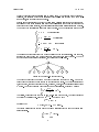
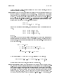
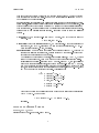
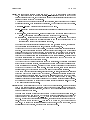

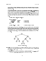
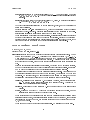
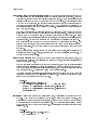

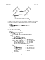
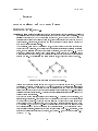
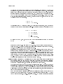
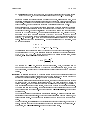
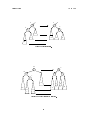

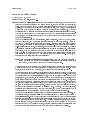

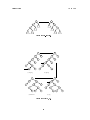

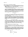

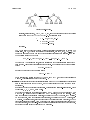

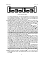

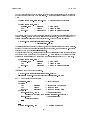


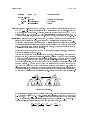
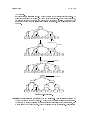
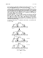
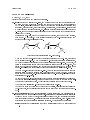
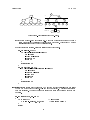

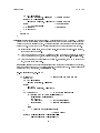
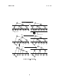
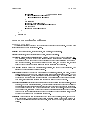
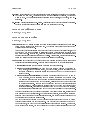
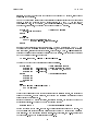
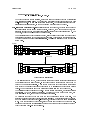
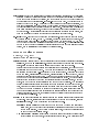
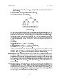
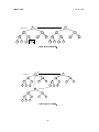
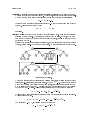
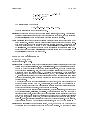
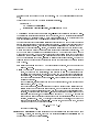
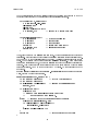
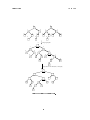

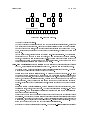
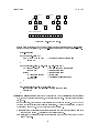
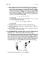
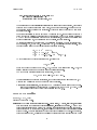
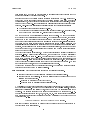
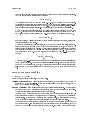
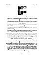
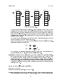
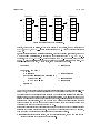
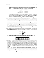
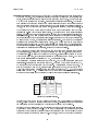

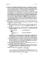

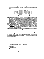
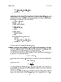
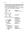
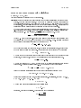
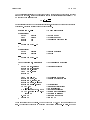
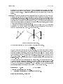

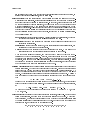
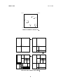

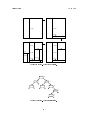
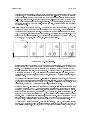
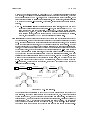
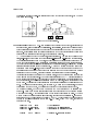

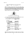
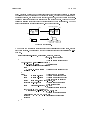
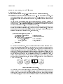

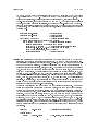
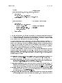
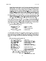

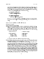

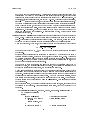


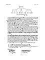

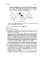
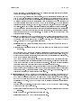
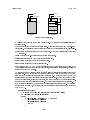

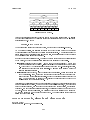
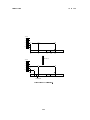
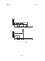
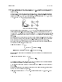
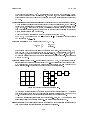
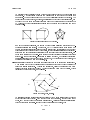

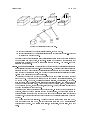
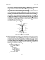
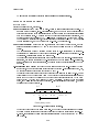
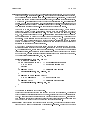
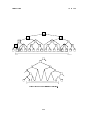
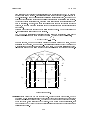

![新製品の特徴[PDF]](http://vs1.manualzilla.com/store/data/006545695_2-9fd79a5ada939bc6e4e47c7aa3d9f1a4-150x150.png)