1
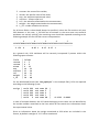
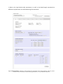
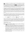
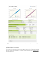
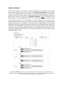
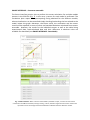
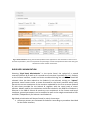
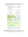
FANTEN web application -‐ USER MANUAL -‐ Introduction FANTEN (see Rinaldelli M, Carlon A et al. J Biomol NMR 61 : 21-‐24) is a new user-‐friendly web tool for the determination of the anisotropy tensors related to PCSs (pseudo-‐contact shifts) and RDCs (residual dipolar couplings), available through the WeNMR portal (http://fanten-‐enmr.cerm.unifi.it:8080). FANTEN is mainly constituted by a first part for the upload of the structure and of the restraints (Fig. 1) (see Input Files), common to all interfaces, and a second part where three different actions can be selected and which are briefly summarized as following: • “PCS-‐RDC Fitting (Custom)” – It allows fully customized calculation of the tensor and, for any dataset, the user can define, if known, metal position, tensor orientation, and anisotropy parameters, or any combination thereof (see CUSTOM INTERFACE); • “PCS-‐RDC Fitting (Smart)” – It allows performing tensor calculation for multiple datasets of PCSs and RDCs and for multiple models present in the PDB file. Moreover, it contains additional functionalities, such as the generation and visualization of the isoPCS surface (in case PCSs are provided), and the estimation of Monte Carlo error on the tensor parameters (see SMART INTERFACE); • “Rigid Body Minimization” – It allows the upload of a second structure and set of restraints, and computes the roto-‐translation to apply to the second structure to obtain the best agreement with the uploaded restraints (see RIGID BODY MINIMIZATION). Input Files The input files consist in (i) a PDB file and (ii-‐a) a PCS and/or (ii-‐b) RDC files: (i) The PDB file can contain different chains as well as different models. It should necessarily contain at least one metal on which the tensor calculation will be performed. In the case in which the position of the tensor is unknown, a dummy atom should be included in the PDB file using unspecified coordinates, as following: HETATM 1204 LA LA A 105 0.000 0.000 0.000 1.00 0.00 LA (ii-‐a) PCS file can be uploaded in PARAMAGNETIC-‐CYANA or in XPLOR-‐NIH formats. For the PARAMAGNETIC-‐CYANA format (see “test_cyana.pcs” in the example files), the attributes related to PCSs are generally reported according to the following order: 1. resnum -‐ the number of the residue, resnam -‐ the name of the residue, atnam -‐ the specific name of the atom, exp -‐ the acquired experimental value, useless -‐ always equal to 1 tol -‐ the tolerance associated to the measurement, weight -‐ the weight associated to the measurement, t_id -‐ a index related to the tensor. For all these fields a value should always be specified, unless the file contains only one PCSs dataset. In this case, t_id field can be omitted. In the case some not essential attributes are entirely missing, the remaining ones should be reported according to the following example line for the their correct interpretation: 1 2 3 4 5 123456789012345678901234567890123456789012345678901234 -‐-‐-‐-‐-‐-‐-‐-‐-‐-‐-‐-‐-‐-‐-‐-‐-‐-‐-‐-‐-‐-‐-‐-‐-‐-‐-‐-‐-‐-‐-‐-‐-‐-‐-‐-‐-‐-‐-‐-‐-‐-‐-‐-‐-‐-‐-‐-‐-‐-‐-‐-‐-‐-‐ 6 LEU H -‐0.03 1 0.15 0.25 1 As a general rule, PCSs attributes will be correctly interpreted if present within the following space columns: Field | Column resnum | 1 -‐ 3 resnam | 4 -‐ 9 atnam | 9 -‐ 12 exp | 16 -‐ 22 useless | 23 -‐ 24 tol | 26 -‐ 31 weight | 32 -‐ 37 t_id | 38 -‐ 40 For the XPLOR-‐NIH format (see “test_xplor.pcs” in the example files), PCSs are reported according to the following syntax: assign ( resid 999 and name OO ) ( resid 999 and name Z ) ( resid 999 and name X ) ( resid 999 and name Y ) ( resid 6 and name HN ) -‐0.4330 0.0000 In case of multiple datasets, the PCS values belonging to the same set are identified by the residue number associated to the lines which do not contain the information about the experimental value. Since no information about the weight associated to PCS values are included in the format, by default a weight of “1.0” will be associated. 2. 3. 4. 5. 6. 7. 8. (ii-‐b) RDC file can be uploaded in PARAMAGNETIC-‐CYANA or in XPLOR-‐NIH format. For the PARAMAGNETIC-‐CYANA format (see “test_cyana.rdc” in the example files), the attributes related to RDCs are generally reported according to the following order: 1. resnum1 -‐ the number of the first residue, 2. atnam1 -‐ the specific name of the atom of the first residue, 3. resnum2 -‐ the number of the second residue, 4. atnam2 -‐ the specific name of the atom of the second residue, 5. exp -‐ the acquired experimental value, 6. t_id -‐ a index related the tensor, 7. tol -‐ the tolerance associated to the measurement, 8. weight -‐ the weight associated to the measurement, 9. freq – the Larmor frequency for the measurement. For all these fields a value should always be specified, except for the attribute freq that, if omitted, is set by default to “700.0”. In the case some not essential attributes are entirely missing, the remaining ones should be reported according to this following example line for their correct interpretation: 1 2 3 4 5 123456789012345678901234567890123456789012345678901234 -‐-‐-‐-‐-‐-‐-‐-‐-‐-‐-‐-‐-‐-‐-‐-‐-‐-‐-‐-‐-‐-‐-‐-‐-‐-‐-‐-‐-‐-‐-‐-‐-‐-‐-‐-‐-‐-‐-‐-‐-‐-‐-‐-‐-‐-‐-‐-‐-‐-‐-‐-‐-‐-‐ 35 N 35 H -‐2.600 3 2.00 0.040 700 As a general rule, RDCs attributes will be correctly read if present within the following space columns: Field | Column resnum1 | 0 -‐ 3 atnam1 | 5 -‐ 7 resnum2 | 9 -‐ 12 atnam2 | 13 -‐ 15 exp | 17 -‐ 25 t_id | 29 – 31 tol | 32 -‐ 37 weight | 41 -‐ 47 freq | 47 -‐ EOL For the XPLOR-‐NIH format (see “test_xplor.rdc” in the example files), RDCs are reported according to the following syntax: assign ( resid 999 and name OO ) ( resid 999 and name Z ) ( resid 999 and name X ) ( resid 999 and name Y ) ( resid 6 and name N ) ( resid 6 and name HN ) -‐5.9590 0.5000 In case of multiple datasets, the RDC values belonging to the same set are identified by the residue number associated to the lines which do not contain the information about the experimental value. Since no information about the weight associated to RDCs are included in the format, by default a weight of “1.0” will be associated. However, for the magnetic field the user should explicitly specify the value in the dedicated text box that will appear upon file upload. The number and the name of the metal used as the position of the tensor can also be included at the end of the PCSs and RDCs file, according to the following syntax: 105 LTNS LA or 105 LTNS In this case, the metal will be automatically associated to the uploaded dataset for the calculation of the tensor. Fig. 1: Interface for the upload of the PDB file and of the NMR restraints. CUSTOM INTERFACE Custom interface is activated selecting “PCS-‐RDC Fitting (Custom)” from the Action Panel (Fig. 2). For each set of PCSs and/or RDCs dataset present in the uploaded files, a different tab is automatically created on which the independent calculation of the tensors may be performed. For each of them, the specific dataset can be chosen, together with the model and the chain (if multiple are present). The set-‐up of the calculation proceeds through three different sections: (i) “METAL POSITION”, (ii) “TENSOR ORIENTATION”, and (iii) “ANISOTROPY VALUES”. (i) The user can operate on the metal position, choosing among three distinct options: • “Unknown”, permits to fit the position of the tensor without any clue about its coordinates and, thus, it will perform a grid search starting from points in the proximity of the protein surface or from atoms constituting its backbone. In particular, the minimization is performed using 8 different starting points for the metal position, corresponding to the vertices of a box containing the protein or randomly choosing 8 atoms belonging to the protein backbone. In most of the cases, 8 starting points are sufficient to estimated with high accuracy the position of the metal ion; • “Choose Metal in pdb file”, permits to choose as tensor position the coordinates associated to a metal present in the PDB file. Moreover, the tensor position can be fixed during the calculation, otherwise optimized freely or imposing an upper bound on its distance from the selected metal; • “Close to Residue in pdb file”, permits to choose as tensor position whatever residue present in the PDB file, and to optimize the position of the tensor starting from that freely or still imposing an upper bound on its distance from the same. (ii) The user can operate on the tensor orientation, choosing among the following options: • “Unknown”, let the tensor orientation to be freely fitted; • “Fix Euler angles”, the tensor orientation can be fixed imposing the Euler angles, according to the selected convention; • “Fix axes from pdb”, the tensor orientation can be fixed selecting the tensor origin and axes orientations as defined by pseudoatoms included in the uploaded PDB (see “test_cyana_with_tensor.pdb” in the example files); • “Fix axes”, the tensor orientation can be fixed manually inserting the eigenvectors of the tensor expressed in its non-‐diagonal matrix form. (iii) The user can operate on the anisotropy values, choosing among the following options: • “Unknown”, let the anisotropy value to be freely fitted; • “Fix Anisotropy values”, permits to fix the anisotropy values. The “GENERAL PARAMETERS” block is used to apply different global weights to PCS and RDC dataset, in case of joint calculation of the tensor, and are set by default to “1.0” for PCSs and to 𝑛𝑜𝑟𝑚(𝑃𝐶𝑆𝑠) 𝑛𝑜𝑟𝑚(𝑅𝐷𝐶𝑠) for RDCs, in such way the two datasets contribute equally during the tensor calculation. Moreover, the temperature expressed in Kelvin, the Lipari-‐Szabo order parameters, as well as the bond length associated to different coupled nuclei can be fixed during the calculation. Fig. 2: Custom Interface. It allows to fully customize the calculation of the tensor defining, if known, metal position, tensor orientation, and anisotropy parameters, or any combination thereof. Note: if a weight of “0.0” is associated to single PCS or RDC values within the provided files, these experimental data will not contribute to the calculation of the tensor. However, their back-‐calculated values will be predicted in any case and represented in the correlation plot using different colours (see “test_cyana_predict.pcs” and “test_cyana_predict.rdc” in the example files). The predicted values are also reported in tabular form at the bottom of the web page together with the fitted values. After the set-‐up, the calculation of the anisotropy tensor can be performed clicking on “Fit Tensor”. Alternatively, the calculation can be performed on all the tensors, after their individual set up, even simultaneously by clicking “Fit all tensors” in the “Global Action” field. Upon checking of “Fit all metals in one position”, the function permits also to perform the calculation of all the tensors using a unique position, that will refer to the one chosen in the first tab. This operation can be useful when the position of the tensor has to be optimized with the constraint that all the tensors should be placed in the same position. For any selected option, FANTEN performs the minimization using the Levenberg-‐ Marquardt algorithm, available from SciPy library, which also permits the inclusion of constraints on the parameters to be optimized in the minimization procedure. A least-‐ squares approach is used to minimize the following target function: 𝑇𝐹 = 𝑘!"# ! 𝑤! 𝑃𝐶𝑆!!"#! − 𝑃𝐶𝑆!!"# ! + 𝑘!"# ! ! 𝑤! 𝑅𝐷𝐶!!"#! − 𝑅𝐷𝐶!!"# where on each PCS or RDC values 𝑤! is the specific weight provided in the uploaded files (if present), and 𝑘!"# (or 𝑘!"# ) indicates the global weight provided through the web interface in the case both PCSs and RDCs are fitted simultaneously. The default values for the global weights for PCSs and RDCs are 1 and the ratio between the norm of vector with components equal to the experimental values of RDCs and of PCSs, respectively. CUSTOM INTERFACE -‐ Results When the calculation of the tensor is complete, the results are shown in the bottom of the page (Fig. 3). For each tensor, are reported: • Correlation plots of the back-‐calculated data against the observed ones, together with the Q-‐factor summarizing the goodness of the fit. The inspection of each represented point can be done upon positioning of the cursor on the data; • Tables showing the calculated tensor values, in terms of axial and rhombic anisotropies, and orientation, expressed in radians and in degree according to the same convention set-‐up before the calculation. The tensor matrix and its eigenvectors are also reported. The triad of axes representing the orientation and the position of the tensors is also reported according to the PDB layout, for easy copy and paste into the file. • Tables listing all the experimental and back-‐calculated data, as well as their difference in absolute value. Fig. 3: Custom Interface. Overview of the results of the fit performed using PCS and RDC datasets. CUSTOM INTERFACE – Downloads The results of the calculation of the tensor together with the list of fitted and predicted data are available for download in .txt format, simply clicking on the “Download Files” and choosing the file. SMART INTERFACE If the tensor position is well known, the Smart interface can be used for easy and fast calculation of several tensors. Upon selection of “PCS-‐RDC Fitting (Smart)” in the Action Panel, a basic interface permits the set-‐up of the calculation operating on the General Parameters field and on the relative weight associated to the PCSs and RDCs datasets, if both present during the upload (see CUSTOM INTERFACE) (Fig. 4). According to the datasets present in the uploaded restraint files, some frames are automatically created representing the tensors. For each of them, the corresponding set of restraint can be associated making use of the t_id reported in the file as well as of the metal choosing among those present in the PDB file. In case both PCSs and RDCs datasets are provided, by default the tensor will be associated to both a set of PCSs and RDCs performing a joint calculation. The independent calculation of the tensors using only PCS or RDC sets can be carried out simply unclicking “JOINT FITTING”, and automatically the frame will split into two frames containing one dataset each. Finally, the calculation will start upon clicking “Perform Action” button. Fig. 4: Smart Interface. It permits to upload multiple PCSs and/or RDCs datasets and determine the anisotropy tensors in a single step. A single anisotropy tensor in best agreement with both PCSs and RDCs can be determined, at will, through the “joint fitting” option. Since metal position is known, Smart Interface allows for a more efficient calculation of the anisotropy tensor, which can be estimated directly by using the following equations (see Bertini I et al., Progress in Magnetic Resonance Spectroscopy 40 : 249-‐273): 𝛿 !"# = 𝛿 !"# = 3𝑘 𝜒!! Where: 1 2𝑧 ! − 𝑥 ! − 𝑦 ! 𝑥! − 𝑦! 2𝑥𝑦 2𝑥𝑧 2𝑦𝑧 𝜒!! + 𝜒!! − 𝜒!! + 𝜒!" ! + 𝜒!" ! + 𝜒!" ! ! ! 4𝜋𝑟 2𝑟 2𝑟 ! 𝑟 𝑟 𝑟 ! ! ! ! ! 2𝑧!" − 𝑥!" − 𝑦!" 𝑥!" − 𝑦!" 2𝑥!" 𝑦!" 2𝑥!" 𝑧!" 2𝑦!" 𝑧!" + 𝜒!! − 𝜒!! + 𝜒!" + 𝜒!" + 𝜒!" ! ! ! ! ! 2𝑟!" 2𝑟!" 𝑟!" 𝑟!" 𝑟!" 𝑘 = − 𝑆!" 𝐵!! 𝛾! 𝛾! ℏ ! 4𝜋 15𝑘𝑇 2𝜋𝑟!" For which the first derivate can be easily obtained and included in a Gauss-‐Newton optimization approach. As for the Custom Interface, the contributions for each restraint are weighted by the specific weight present in the file, and by the global weight inserted in the dedicated textbox present in the interface. In case of joint estimation of the tensor using both PCSs and RDCs, the tensor related to RDCs is scaled by a factor equal to the model-‐free order parameter, which can be directly modified in the “General Parameters” field present in the interface. SMART INTERFACE -‐ Results After the calculation is complete, the results will be reported as explained in Custom Interface. In addiction to the tabs showing the data for each tensor, the “Tensor All” tab is generated reporting the superimposing correlation plots of the calculated tensors together with the global Q-‐factor (Fig. 5). Global Q-‐factor in calculated as a usual Q-‐factor on all the experimental data. Fig. 5: Smart Interface. It automatically generates a summary of all calculated tensors, including the plots showing the agreement between experimental and calculated data for the different tensors. When RDCs arising from partial alignment induced by external orienting media are provided, the results of the calculation are given in terms of alignment tensors (Fig. 6). As mentioned in the methods section, the size of the tensors is provided by their magnitude A and rhombicity R, defined as: 𝐴!! − 𝐴!! 3 𝐴 = 𝐴!! , 𝑅 = 2 𝐴 where 𝐴!! are the components of the A tensor in the frame where it is diagonal. For the sake of completeness, also the maximum RDC induced N-‐NH nuclear pair (DNH) is reported (see Tjandra N. & Bax A. Science 278 : 1111-‐1114): 𝐷!" = − 𝑆!" 𝜇! 𝛾! 𝛾! ℎ 𝐴 ! 16𝜋 ! 𝑟!" Fig 6: Smart Interface. For RDCs arising from external alignment media the size of the tensors is provided by their magnitude A, the rhombicity R, and the maximum DNH value. SMART INTERFACE – Structures ensemble The Smart Interface permits also to perform the tensor calculation for multiple models present in the PDB file (Fig. 7). In this case, a tensor for each model is estimated. The correlation plots report the superimposing fitting obtained for the different models, whose visualization can be controlled simply checking/unchecking the box related to the model, below the graph. Moreover, the tensor value, the orientation and the tensor matrix will be reported in terms of mean and standard deviation calculated from tensors ensemble. However, the results for the individual tensors as well as the table listing experimental data, back-‐calculated data and their difference in absolute value are available for download (see SMART INTERFACE -‐ Downloads). Fig. 7: Smart Interface. When a structural ensemble is provided as input, a tensor for each model contained in the PDB is estimated, and Δχax and Δχrh, values, the Euler angles and the tensor matrices are reported in terms of average and standard deviation obtained from the different models. SMART INTERFACE – JSmol web application Smart Interface offers the additional functionality for graphical visualization of the isoPCS surfaces computed for each tensor, by using an integrated JSmol web application. Clicking on “Visualize Tensor”, a window opens in which the uploaded protein together with the isoPCS surface with threshold of 1.0 are graphically represented (Fig.8). The isoPCS surface in .cube format is also available for download. Fig. 8: Smart Interface. The isoPCS surface (with threshold equal to 1 ppm) superimposed to the protein chain can be visualized through an integrated JSmol applet. SMART INTERFACE – Monte Carlo Statistics Smart Interface presents at the bottom page the possibility to perform the estimates of the error on the computed tensor parameters using a Monte Carlo bootstrap approach (Fig. 9). The user may decide the percentage of retained experimental data during the calculation as well as the number of iterations. The tensor values, orientations and tensor matrix are reported in terms of mean and standard deviation. SMART INTERFACE – Downloads The results of the calculation of the tensor together with the list of fitted and predicted data are available for download in .txt format, simply clicking on the “Download Files” and choosing the file. Moreover, in case at least one PCSs dataset is provided, the isoPCS surface in .cube format is also available for download and can be easily open and visualized using common visualization software, such as PyMol and UCSF Chimera. From “Tensor All” tab, it is also possible to download the files summarizing the results obtained by the calculation of all the tensors. Fig. 9: Smart Interface. During the a bootstrap Monte Carlo approach for the estimation of the errors on the best fit parameters, the user may decide the percentage of retained experimental data used during the calculation and the number of iterations. RIGID BODY MINIMIZATION Selecting “Rigid Body Minimization” in the Action Panel, the upload of a second structure (Subunit B) as well as of a second set of restraints is possible (Fig. 10). Similarly to the Custom interface, model and chain considered during the calculation should be selected. Once the data related to the Subunit B are selected, clicking on “Upload” generates some frames similar to those discussed for the Smart Interface which easily permits the correct association of the restraints uploaded for the first structure (Subunit A) with those provided for the Subunit B, together with the metal used as tensor position. Metals used for the calculation should be included in the PDB file of Subunit A, whereas in the PDB of Subunit B metals are not considered. As for Custom and Smart Interfaces, general parameters can be modified as well as the weight associated to PCSs and RDCs, independently for Subunit A and Subunit B. Rigid body minimization will be performed in mainly three steps: 1. Anisotropy tensors are estimated for Subunit A according to procedure described for the Smart Interface; 2. A roto-‐traslation is computed in such a way to find the best agreement between the experimental data provided for Subunit B and those back-‐calculated using the anisotropy tensors estimated for Subunit A; 3. Once the roto-‐traslation has been applied to Subunit B, new calculation of the tensors is performed using both sets of restraints. Fig. 10: Rigid Body Minimization Interface. After the upload of the first molecular structure (Subunit A) and the related experimental datasets, a second molecular structure (Subunit B) and the corresponding PCS/RDC datasets can be provided. The datasets for the two subunits corresponding to the same tensors can be paired and associated to the corresponding metals, the coordinates of which must be provided in the PDB file related to the Subunit A. The estimate of a roto-‐translation of a molecular structure can be considered as a general rigid body movement problem that can be expressed according to the following least-‐squares problem: min!∈!,! ! !!! 𝑅𝑥! + 𝑑 − 𝑦! (Eq.1) where 𝑅 and 𝑑 are, respectively, the rotation matrix and the translation vector that map the points 𝑥! to the points 𝑦! , 𝑛 = 1, . . . , 𝑛. In the particular case of finding the optimal arrangement between two molecular structures by using PCS and RDC restraints, 𝑅 and 𝑑 can be determined by making use of the following algorithm: 1. Fitting of the tensor parameters for the Subunit A; 2. Fitting of the tensor parameters (and of its position) for the Subunit B, by making use of the anisotropy values estimated for the Subunit A; 3. Two sets A and B of points are created comprising the coordinates of the tensor axes (the center and the three vertices of the unit axes) of the Subunits A and B, such that: 𝐴 = 𝑥! , … , 𝑥! , 𝐵 = 𝑦! , … , 𝑦! 4. Since Eq.1 is linear with respect to the vector d, the centroid of each set of points (𝑥 and 𝑦) can be computed and subtracted to sets A and B, as following: 𝐴 = 𝑥! − 𝑥, … , 𝑥! − 𝑥 , 𝐵 = 𝑦! − 𝑦, … , 𝑦! − 𝑦 thus reducing the least-‐squares problem expressed in Eq.1 to: min!∈! ! !!! 𝑅𝐴 − 𝐵 ! (Eq.2) where 𝑅𝐴 − 𝐵 ! indicates the Frobenius norm of the matrix. The problem in Eq.2 defines an Orthogonal Procrustes problem that can be solved by making use a Singular Value Decomposition (SVD) approach (see Schönemann PH. Psychometrika 33 : 19-‐33); 5. Once the center of mass has been subtracted, the rotation matrix 𝑅 can be easily determined as: 𝑅 = 𝑈 𝑑𝑖𝑎𝑔 1, 1, det 𝑈 𝑉 ! 𝑉 ! where: 𝑈 𝑆 𝑉 ! = 𝐵 𝐴! 6. Finally, the translation vector 𝑑 can be retrieved as: 𝑑 = 𝑦 − 𝑅𝑥 In case multiple tensors are available for the determination of the roto-‐translation, sets A and B are collections of points describing the axes orientation of all the tensors. In this way, a “global” rotation matrix and translation vector is estimated able to optimally superimpose the collections of tensors estimated for Subunits A and B (Fig.11-‐A). Subunit B Subunit B rototranslated Subunit B (Solution 2) Subunit B (Solution 3) Subunit A Subunit A A B Subunit B (Solution 1) Subunit B (Solution 4) Fig. 11: Rigid Body Minimization. In case of multiple tensors, a single roto-‐translated version of Subunit B is found (panel A), whereas in case of a single tensor four equally possible solutions are found (panel B). Special consideration requires the case in which Rigid Body Minimization is performed using only one tensor. In this case, due to the intrinsic ambiguity of this mathematic problem, four equivalent solutions in terms of arrangement between Subunit A and Subunit B are possible (Fig.11-‐B). Thus, four roto-‐translated versions of Subunit B are generated and available for download. Note: roto-‐translation is computed only when at least one PCS dataset is provided, otherwise only the orientation of Subunit B will be optimized. Note: if arrangement of Subunits A and B needs only to be slightly optimized respect to the starting one, “Perform gridsearch algorithm” option can be avoided. In case the position of the metal for Subunit B is completely unknown, the gridsearch approach is recommended. RIGID BODY MINIMIZATION – Results After the minimization is performed the results for each tensor (Fig. 12) are reported as following: • Correlation plots of the back-‐calculated data against the observed ones, together with the Q-‐factor summarizing the goodness of the fit are shown for both Subunit A and Subunit B; • Tables showing the calculated tensor values, in terms of axial and rhombic anisotropies, and orientation, expressed in radians and in degree according to the same convention set-‐up before the calculation. The tensor matrix and its eigenvectors are also reported. The triad of axes representing the orientation and the position of the tensors is also reported according to the PDB layout, for easy copy and past of the file; • • The transformation applied to Subunit B to obtain the best agreement with the experimental data, in terms of translation vector and rotation matrix; Tables listing all the experimental and back-‐calculated data, as well as their difference in absolute value. Fig. 12: Rigid Body Minimization Interface. It provides as output the anisotropy parameter, the values of the Euler angles, the tensor matrices and the eigenvectors providing the main axes of the tensor together with the plots showing the agreement between experimental and back-‐calculated data for both Subunit A and Subunit B, and also the information about the applied transformation. RIGID BODY MINIMIZATION – Downloads The results of the calculation of the tensor together with the list of fitted and predicted data for both Subunit A and B are available for download in .txt format, simply clicking on the “Download Files” and choosing the file. The minimized version of the Subunit B is also available for download. In case only one tensor is used during the rigid body minimization algorithm, all the four possible roto-‐translated versions of Subunit B are available for download. FANTEN CONVENTIONS FANTEN – Convention in choosing the tensor In the general case, the axis of the anisotropy tensor is not uniquely determined and, in particular, three equally acceptable solutions can be found. FANTEN selects the solution that simultaneously satisfies the two following criteria: a. 𝜒!! ≤ 𝜒!! ≤ 𝜒!! b. Δ𝜒!! ≤ 2 3 Δ𝜒!" FANTEN – Euler angles convention Euler angles convention to be used in FANTEN can be chosen between the available ones in the “General Parameters” field for the Smart Interface and Rigid Body Docking, or in the “TENSOR ORIENTATION” section from the Custom Interface. The selected convention will be used by the program that after the tensor estimation will report the results in term of Euler angles according to the same convention. In particular, the Euler angles convention is defined by a 4-‐character string, in which the first character defines if rotations are applied to static (s) or rotating (r) frame, whereas the remaining three characters specify the axes about which the three consecutive rotations occur. The resulting transformation matrix represents the rotation that brings the reference system to coincide with the principal axis system of the anisotropy tensor (passive rotation). As example, in the “szyz” convention, where three consecutive rotations of α, β and γ about the fixed initial z, y and z axes, respectively, of the reference frame occur, the rotation matrix is: cos 𝛼 cos 𝛽 cos 𝛾 − sin 𝛼 sin 𝛾 𝑅 = cos 𝛼 cos 𝛽 sin 𝛾 + sin 𝛼 cos 𝛾 − cos 𝛼 sin 𝛽 − sin 𝛼 cos 𝛽 cos 𝛾 − cos 𝛼 sin 𝛾 − sin 𝛼 cos 𝛽 sin 𝛾 + cos 𝛼 cos 𝛾 sin 𝛼 sin 𝛽 CONTACT For any help, please contact me at: [email protected] sin 𝛽 cos 𝛾 sin 𝛽 sin 𝛾 cos 𝛽