Download EC-Lab User`s Manual

EC-Lab
Software
User's Manual
Version 10.38 – August 2014
Equipment installation
WARNING!: The instrument is safety ground to the Earth through the protective conductor of the AC power cable.
Use only the power cord supplied with the instrument and designed for the good current
rating (10 Amax) and be sure to connect it to a power source provided with protective
earth contact.
Any interruption of the protective earth (grounding) conductor outside the instrument
could result in personal injury.
Please consult the installation manual for details on the installation of the instrument.
General description
The equipment described in this manual has been designed in accordance with EN61010 and
EN61326 and has been supplied in a safe condition. The equipment is intended for electrical
measurements only. It should be used for no other purpose.
Intended use of the equipment
This equipment is an electrical laboratory equipment intended for professional and intended to
be used in laboratories, commercial and light-industrial environments. Instrumentation and accessories shall not be connected to humans.
Instructions for use
To avoid injury to an operator the safety precautions given below, and throughout the manual,
must be strictly adhered to, whenever the equipment is operated. Only advanced user can use
the instrument.
Bio-Logic SAS accepts no responsibility for accidents or damage resulting from any failure to
comply with these precautions.
GROUNDING
To minimize the hazard of electrical shock, it is essential that the equipment be connected to
a protective ground through the AC supply cable. The continuity of the ground connection
should be checked periodically.
ATMOSPHERE
You must never operate the equipment in corrosive atmosphere. Moreover if the equipment is
exposed to a highly corrosive atmosphere, the components and the metallic parts can be corroded and can involve malfunction of the instrument.
The user must also be careful that the ventilation grids are not obstructed. An external
cleaning can be made with a vacuum cleaner if necessary.
Please consult our specialists to discuss the best location in your lab for the instrument (avoid
glove box, hood, chemical products, …).
AVOID UNSAFE EQUIPMENT
The equipment may be unsafe if any of the following statements apply:
- Equipment shows visible damage,
- Equipment has failed to perform an intended operation,
- Equipment has been stored in unfavourable conditions,
- Equipment has been subjected to physical stress.
In case of doubt as to the serviceability of the equipment, don’t use it. Get it properly checked
out by a qualified service technician.
LIVE CONDUCTORS
When the equipment is connected to its measurement inputs or supply, the opening of covers
or removal of parts could expose live conductors. Only qualified personnel, who should refer
to the relevant maintenance documentation, must do adjustments, maintenance or repair
EQUIPMENT MODIFICATION
To avoid introducing safety hazards, never install non-standard parts in the equipment, or
make any unauthorised modification. To maintain safety, always return the equipment to
Bio-Logic SAS for service and repair.
GUARANTEE
Guarantee and liability claims in the event of injury or material damage are excluded when
they are the result of one of the following.
- Improper use of the device,
- Improper installation, operation or maintenance of the device,
- Operating the device when the safety and protective devices are defective
and/or inoperable,
- Non-observance of the instructions in the manual with regard to transport,
storage, installation,
- Unauthorized structural alterations to the device,
- Unauthorized modifications to the system settings,
- Inadequate monitoring of device components subject to wear,
- Improperly executed and unauthorized repairs,
- Unauthorized opening of the device or its components,
- Catastrophic events due to the effect of foreign bodies.
IN CASE OF PROBLEM
Information on your hardware and software configuration is necessary to analyze and finally
solve the problem you encounter.
If you have any questions or if any problem occurs that is not mentioned in this document,
please contact your local retailer (list available following the link: http://www.bio-logic.info/potentiostat/distributors.html). The highly qualified staff will be glad to help you.
Please keep information on the following at hand:
- Description of the error (the error message, mpr file, picture of setting or any
other useful information) and of the context in which the error occurred. Try
to remember all steps you had performed immediately before the error occurred. The more information on the actual situation you can provide, the
easier it is to track the problem.
- The serial number of the device located on the rear panel device.
Model: VMP3
s/n°: 0001
Power: 110-240 Vac 50/60 Hz
Fuses: 10 AF Pmax: 650 W
-
The software and hardware version you are currently using. On the Help
menu, click About. The displayed dialog box shows the version numbers.
The operating system on the connected computer.
The connection mode (Ethernet, LAN, USB) between computer and instrument.
General safety considerations
The instrument is safety ground to the Earth through
the protective conductor of the AC power cable.
Class I
Use only the power cord supplied with the instrument
and designed for the good current rating (10 A max) and
be sure to connect it to a power source provided with
protective earth contact.
Any interruption of the protective earth (grounding)
conductor outside the instrument could result in personal injury.
Guarantee and liability claims in the event of injury or material damage are excluded when they are the result of one of
the following.
- Improper use of the device,
- Improper installation, operation or maintenance of the
device,
- Operating the device when the safety and protective devices are defective and/or inoperable,
- Non-observance of the instructions in the manual with
regard to transport, storage, installation,
- Unauthorised structural alterations to the device,
- Unauthorised modifications to the system settings,
- Inadequate monitoring of device components subject to
wear,
- Improperly executed and unauthorised repairs,
- Unauthorised opening of the device or its components,
- Catastrophic events due to the effect of foreign bodies.
ONLY QUALIFIED PERSONNEL should operate (or service) this equipment.
EC-Lab Software User's Manual
Table of contents
Equipment installation ............................................................................................. i
General description ................................................................................................. i
Intended use of the equipment ................................................................................ i
Instructions for use .................................................................................................. i
General safety considerations ............................................................................... iv
1.
Introduction................................................................................................................... 6
2.
EC-Lab software: settings .......................................................................................... 8
2.1
Starting EC-Lab .................................................................................................... 8
2.2
EC-Lab Main Menu ............................................................................................. 11
2.3
Tool Bars .............................................................................................................. 14
2.3.1 Main Tool Bar.................................................................................................... 14
2.3.2 Channel tool bar................................................................................................ 15
2.3.3 Graph Tool Bar ................................................................................................. 16
2.3.4 Status Tool Bar ................................................................................................. 16
2.3.5 Current Values Tool Bar .................................................................................... 16
2.4
Devices box .......................................................................................................... 17
2.5
Experiments box................................................................................................... 18
2.5.1 Parameters Settings Tab................................................................................... 18
2.5.1.1 Right-click on the “Parameters Settings” tab .............................................. 18
2.5.1.2 Selecting a technique ................................................................................ 19
2.5.1.3 Changing the parameters of a technique ................................................... 21
2.5.2 Cell Characteristics Tab .................................................................................... 25
2.5.2.1 Cell Description ......................................................................................... 26
2.5.2.1.1 Standard “Cell Description” frame ........................................................ 26
2.5.2.1.2 Battery “Cell Description” frame ........................................................... 27
2.5.2.2 Reference electrode .................................................................................. 28
2.5.2.3 Record ...................................................................................................... 29
2.5.3 Advanced Settings tab ...................................................................................... 29
2.5.3.1 Advanced Settings with VMP3, VSP, SP-50, SP-150 ................................ 30
2.5.3.1.1 Compliance.......................................................................................... 30
2.5.3.1.2 Safety Limits ........................................................................................ 31
2.5.3.1.3 Electrode Connections ......................................................................... 32
2.5.3.1.4 Miscellaneous ...................................................................................... 32
2.5.3.2 Advanced Settings with HCP-803, HCP-1005, CLB-500 and CLB-2000 .... 33
2.5.3.3 Advanced Settings with MPG-2XX ............................................................ 34
2.5.3.4 Advanced Settings for SP-200, SP-240, SP-300, VSP-300, VMP-300 ...... 35
2.5.3.4.1 Filtering................................................................................................ 36
2.5.3.4.2 Channel ............................................................................................... 36
2.5.3.4.3 Ultra Low Current Option ..................................................................... 36
2.5.3.4.4 Electrode Connections ......................................................................... 38
2.6
Accepting and saving settings and running a technique ....................................... 40
2.6.1 Accepting and saving settings ........................................................................... 40
2.6.2 Running an experiment ..................................................................................... 40
2.7
Linking techniques ................................................................................................ 41
2.7.1 Description and settings .................................................................................... 41
2.7.2 Applications....................................................................................................... 43
2.7.2.1 Linked experiments with EIS techniques ................................................... 43
2.7.2.2 Application of linked experiments with ohmic drop compensation .............. 45
1
EC-Lab Software User's Manual
2.8
Available commands during the run...................................................................... 46
2.8.1 Stop and Pause ................................................................................................ 46
2.8.2 Next Technique/Next Sequence ........................................................................ 46
2.8.3 Modifying an experiment in progress ................................................................. 47
2.8.4 Repair channel .................................................................................................. 47
2.8.5 Use of the Repair channel tool .......................................................................... 48
2.9
Multi-channel selection: Grouped, Synchronized Stacked or bipotentiostat
experiments ...................................................................................................................... 50
2.9.1 Grouped or synchronized experiments .............................................................. 50
2.9.2 Stack experiments............................................................................................. 52
2.10 Batch mode .......................................................................................................... 55
2.11 Data properties ..................................................................................................... 57
2.11.1
Type of data files ........................................................................................... 57
2.11.2
Variables description ..................................................................................... 57
2.11.3
Data recording............................................................................................... 59
2.11.4
Data saving ................................................................................................... 60
2.12 Changing the channel owner ................................................................................ 60
2.13 Virtual potentiostat ................................................................................................ 61
2.14 Configuration options............................................................................................ 61
2.14.1
General Options ............................................................................................ 62
2.14.2
Warning Options ........................................................................................... 63
2.14.3
Text Export Options....................................................................................... 64
2.14.4
Color Options ................................................................................................ 64
2.14.5
References Options....................................................................................... 65
2.14.6
Tool bars/menus Options .............................................................................. 66
2.14.7
E-mail/menus Options ................................................................................... 67
3.
EC-Lab software: Graphic Display........................................................................... 69
3.1
Graphic window .................................................................................................... 69
3.1.1 Loading a data file ............................................................................................. 71
3.1.2 EC-Lab graphic display ................................................................................... 73
3.1.3 Graphic tool bar ................................................................................................ 74
3.1.4 Data file and plot selection window ................................................................... 74
3.2
Graphic tools ........................................................................................................ 76
3.2.1 Cycles/Loops visualization ................................................................................ 76
3.2.2 Show/Hide points .............................................................................................. 77
3.2.3 Add comments on the graph ............................................................................. 77
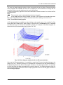
3.2.4 Three-Dimensional graphic ............................................................................... 79
3.2.5 Graph properties ............................................................................................... 80
3.2.6 LOG (History) file .............................................................................................. 83
3.2.7 Copy options ..................................................................................................... 85
3.2.7.1 Standard copy options ............................................................................... 85
3.2.7.2 Advanced copy options ............................................................................. 85
3.2.8 Print options ...................................................................................................... 85
3.2.9 Multi-graphs in a window ................................................................................... 87
3.2.9.1 Multi windows ............................................................................................ 87
3.2.10
Graph Representation menu ......................................................................... 88
3.2.10.1
Axis processing ..................................................................................... 89
3.2.10.2
How to create your own graph representation for a specific technique? 90
3.2.10.3
How to create a Graph Style? ................................................................ 91
4.
2
Analysis....................................................................................................................... 94
EC-Lab Software User's Manual
4.1
Math Menu ........................................................................................................... 94
4.1.1 Min and Max determination ............................................................................... 95
4.1.2 Linear Fit ........................................................................................................... 96
4.1.3 Polynomial Fit ................................................................................................... 97
4.1.4 Circle Fit ............................................................................................................ 97
4.1.5 Linear Interpolation ........................................................................................... 98
4.1.6 Subtract Files .................................................................................................... 99
4.1.7 Integral ............................................................................................................ 100
4.1.8 Fourier Transform ........................................................................................... 101
4.1.9 Filter ................................................................................................................ 102
4.1.10
Multi-Exponential Sim/Fit ............................................................................. 103
4.2
General Electrochemistry Menu ......................................................................... 104
4.2.1 Peak Analysis ................................................................................................. 104
4.2.1.1 Baseline selection ................................................................................... 105
4.2.1.2 Peak analysis results ............................................................................... 106
4.2.1.3 Results of the peak analysis using a linear regression baseline .............. 106
4.2.1.4 Results of the peak analysis using a polynomial baseline ........................ 107
4.2.2 Wave analysis ................................................................................................. 108
4.2.3 CV Sim............................................................................................................ 108
4.2.4 CV Fit .............................................................................................................. 113
4.2.4.1 Mechanism tab ........................................................................................ 114
4.2.4.2 Setup tab ................................................................................................. 115
4.2.4.3 Selection tab ........................................................................................... 116
4.2.4.4 Fit tab ...................................................................................................... 117
4.2.4.5 CV Fit bottom buttons .............................................................................. 118
4.2.4.6 CV Fit results ........................................................................................... 119
4.3
Electrochemical Impedance Spectroscopy menu ............................................... 120
4.3.1 Z Fit: Electrical equivalent elements ................................................................ 120
4.3.1.1 Resistor: R .............................................................................................. 121
4.3.1.2 Inductor: L ............................................................................................... 121
4.3.1.3 Modified Inductor: La................................................................................ 122
4.3.1.4 Capacitor: C ............................................................................................ 123
4.3.1.5 Constant Phase Element: Q .................................................................... 123
4.3.1.6 Warburg element for semi-infinite diffusion: W......................................... 124
4.3.1.7 Warburg element for convective diffusion: W d ......................................... 124
4.3.1.8 Restricted diffusion element: M ............................................................... 125
4.3.1.9 Modified restricted diffusion element: Ma ................................................. 126
4.3.1.10
Anomalous diffusion element or Bisquert diffusion element: Mg ........... 126
4.3.1.11
Gerischer element: G........................................................................... 127
4.3.1.12
Modified Gerischer element #1: Ga ...................................................... 127
4.3.1.13
Modified Gerischer element #2: Gb ...................................................... 128
4.3.2 Simulation: Z Sim ............................................................................................ 129
4.3.2.1 Z Sim window .......................................................................................... 129
4.3.2.2 Circuit selection ....................................................................................... 131
4.3.2.2.1 Circuit description .............................................................................. 131
4.3.3 Fitting: Z Fit ..................................................................................................... 133
4.3.3.1 Equivalent circuit frame ........................................................................... 134
4.3.3.2 The Fit frame ........................................................................................... 134
4.3.3.3 Application ............................................................................................... 136
4.3.3.4 Fit on successive cycles .......................................................................... 138
4.3.3.4.1 Pseudo-capacitance .......................................................................... 139
4.3.3.4.2 Additional plots .................................................................................. 140
4.3.4 Mott-Schottky Fit ............................................................................................. 142
4.3.4.1 Mott-Schottky relationship and properties of semi-conductors ................. 142
3
EC-Lab Software User's Manual
4.3.4.2 The Mott-Schottky plot............................................................................. 142
4.3.4.3 The Mott-Schottky Fit .............................................................................. 143
4.3.4.4 Saving Fit and analysis results ................................................................ 145
4.3.5 Kramers-Kronig transformation ....................................................................... 146
4.4
Batteries menu ................................................................................................... 147
4.5
Photovoltaic/fuel cell menu ................................................................................. 147
4.5.1 Photovoltaic analysis… ................................................................................... 148
4.6
Supercapacitor menu ......................................................................................... 148
4.7
Corrosion menu .................................................................................................. 148
4.7.1 Tafel Fit ........................................................................................................... 149
4.7.1.1 Tafel Fit window ...................................................................................... 150
4.7.1.2 Corrosion rate.......................................................................................... 152
4.7.1.3 Minimize option ....................................................................................... 152
4.7.2 Rp Fit ............................................................................................................... 153
4.7.3 Corr Sim.......................................................................................................... 155
4.7.4 Variable Amplitude Sinusoidal microPolarization Fit (VASP Fit) ...................... 155
4.7.5 Constant Amplitude Sinusoidal microPolarization Fit (CASP Fit) ..................... 156
4.7.6 Electrochemical Noise Analysis....................................................................... 158
4.7.7 Other corrosion processes .............................................................................. 159
5.
Data and file processing .......................................................................................... 160
5.1
Data processing ................................................................................................. 160
5.1.1 Process window .............................................................................................. 160
5.1.2 Additional processing options .......................................................................... 162
5.1.3 The derivative process .................................................................................... 163
5.1.4 The compact process ...................................................................................... 164
5.1.5 Capacity and energy per cycle and sequence ................................................. 165
5.1.6 Summary per protocol and cycle ..................................................................... 167
5.1.7 Constant power protocol summary .................................................................. 168
5.1.8 Coulombic Efficiency Determination (CED Fit) ................................................ 169
5.1.9 Polarization Resistance ................................................................................... 171
5.1.10
Multi-Pitting Statistics .................................................................................. 173
5.2
Data File import/export functions ........................................................................ 174
5.2.1 ASCII text file creation and exportation ........................................................... 174
5.2.2 ZSimpWin exportation ..................................................................................... 175
5.2.3 ASCII text file importation from other electrochemical software ....................... 175
5.2.4 FC-Lab data files importation .......................................................................... 177
6.
Advanced features.................................................................................................... 178
6.1
Maximum current range limitation (2.4 A) on the standard channel board .......... 178
6.1.1 Different limitations.......................................................................................... 178
6.1.2 Application to the GSM battery testing ............................................................ 179
6.2
Optimization of the potential control resolution ................................................... 181
6.2.1 Potential Control range (span) ........................................................................ 181
6.2.2 Settings of the Working Potential window ........................................................ 182
6.3
Measurement versus control current range ........................................................ 183
6.3.1 The potentio mode .......................................................................................... 183
6.3.2 The galvano mode .......................................................................................... 184
6.3.3 Particularity of the 1 A current range in the galvano mode .............................. 184
6.3.4 Multiple current range selection in an experiment ........................................... 185
6.4
External device control and recording ................................................................. 185
4
EC-Lab Software User's Manual
6.4.1 General description ......................................................................................... 185
6.4.2 Rotating electrodes control.............................................................................. 187
6.4.2.1 Control panel ........................................................................................... 189
6.4.3 Temperature control ........................................................................................ 191
6.4.4 Electrochemical Quartz Crystal Microbalance coupling ................................... 192
7.
Troubleshooting ....................................................................................................... 194
7.1
7.2
7.3
Data saving ........................................................................................................ 194
PC Disconnection ............................................................................................... 194
Effect of computer save options on data recording ............................................. 194
8.
Glossary .................................................................................................................... 195
9.
Index .......................................................................................................................... 201
5
EC-Lab Software User's Manual
1.
Introduction
EC-Lab software has been designed and built to control all our potentiostats (single channel:
SP-50, SP-150, HCP-803, HCP-1005, CLB-2000, SP-300, SP-200, SP-240 or multichannels:
VMP2(Z), VMP3, MPG-2XX series, VSP, VSP-300 and VMP-300. Each channel board of our
multichannel instruments is an independent potentiostat/galvanostat that can be controlled by
EC-Lab software.
Each channel can be set, run, paused or stopped, independently of each other, using identical
or different protocols. Any settings of any channel can be modified during a run, without interrupting the experiment. The channels can be interconnected and run synchronously, for example to perform multi-pitting experiments using a common counter-electrode in a single bath.
One computer (or eventually several for multichannel instruments) connected to the instrument
can monitor the system. The computer can be connected to the instrument through an Ethernet
connection or with an USB connection. With the Ethernet connection, each one of the users is
able to monitor his own channel from his computer. More than multipotentiostats, our instruments are modular, versatile and flexible multi-user instruments. Additionally, thanks to the
multiconnection, several instruments can be controlled by one computer with only one EC-Lab
session open.
Once the protocols have been loaded and started from the PC, the experiments are entirely
controlled by the on-board firmware of the instrument. Data are temporarily buffered in the
instrument and regularly transferred to the PC, which is used for data storage, on-line visualization and off-line data analysis and display.
This architecture ensures very safe operations since a shutdown of the monitoring PC does
not affect the experiments in progress.
The application software package provides useful protocols for general electrochemistry, corrosion, batteries, super-capacitors, fuel cells and custom applications. Usual electrochemical
techniques, such as Cyclic Voltammetry, Chronopotentiometry, etc…, are obtained by associations of elementary sequences.
Conditional tests can be performed at various levels of any sequence on the working electrode
potential or current, on the counter electrode potential, or on the external parameters. These
conditional tests force the experiment to go to the next step or to loop to a previous sequence
or to end the sequence.
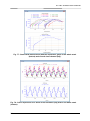
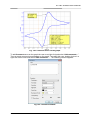
Standard graphic functions such as re-scaling, zoom, linear and log scales are available. The
user can also overlay curves to make data analyses (peak and wave analysis, Tafel, Rp, linear
fits, EIS simulation and modeling, …).
Post-processing is possible using built-in options to create variables at the user's convenience,
such as derivative or integral values, etc... Raw data and processed data can be exported as
standard ASCII text files.
The aim of this manual is to guide the user in EC-Lab software discovery. This manual is
composed of several chapters. The first is an introduction. The second and third parts describe
the software and give an explanation of the different techniques and protocols offered by ECLab. Finally, some advanced features and troubleshooting are described in the two last parts.
6
EC-Lab Software User's Manual
The other supplied manual “EC-Lab Software Techniques and Applications” is aimed at describing in detail all the available techniques.
It is assumed that the user is familiar with Microsoft Windows© and knows how to use the
mouse and keyboard to access the drop-down menus.
WHEN AN USER RECEIVES A NEW UNIT FROM THE FACTORY, THE SOFTWARE AND FIRMWARE ARE
INSTALLED AND UPGRADED. THE INSTRUMENT IS READY TO BE USED. IT DOES NOT NEED TO BE UPGRADED. W E ADVISE THE USERS TO READ AT LEAST THE SECOND AND THIRD CHAPTERS BEFORE
STARTING AN EXPERIMENT.
7
EC-Lab Software User's Manual
2.
EC-Lab software: settings
At this point, the installation manual of your instrument has been carefully read and the
user knows how to connect his/her instrument to the potentiostat. The several steps of
the connection will not be described in this manual but in the installation manual of the
instrument.
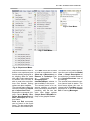
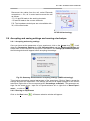
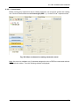
2.1 Starting EC-Lab
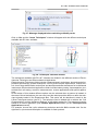
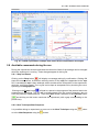
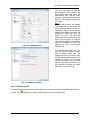
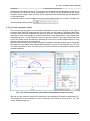
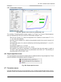
Double click on the EC-Lab icon on the desktop, EC-Lab opens and connects to an instrument. See the Instrument’s Manuals for more details about the instruments connection. Once
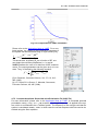
an instrument is connected to EC-Lab the main window will be displayed:
Fig. 1: Starting main EC-Lab window.
If the computer is connected to the Internet, a Newsletter appears.
Furthermore, on the left column, two boxes can be seen:
Devices box that lists the instruments to which the computer can be connected. For
more information on this box, please see the Instrument’s Manual.
Experiment that lists the series of techniques that are used to perform the desired experiment on the selected channel of the selected instrument.
8
EC-Lab Software User's Manual
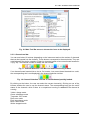
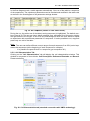
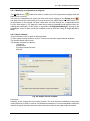
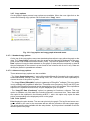
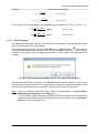
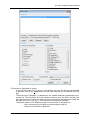
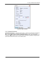
When EC-Lab is connected to an instrument the following Username window can be seen:
Fig. 2: User name window.
Type your username (example: My Name), and click OK or press < ENTER >.
This User Name is used as a safety password when the instrument is shared between several
users. When you run an experiment on a channel, this code will be automatically transferred
to the section "user" on the bottom of EC-Lab software window. This allows the user to become the owner of the channel for the duration of the experiment. All users are authorized to
view the channels owned by the other users. However, change of parameters on a channel is
authorized only if the present User Name corresponds to the owner of that channel (even from
another computer). If another user wants to modify parameters on a channel that belongs to
"My Name", the following message appears:
"Warning, channel X belongs to "My Name". By accepting modification you will replace
current owner. Do you want to continue?"
The command User... in the Config. menu allows you to change the User Name at any time.
You can also double click on the “User“section in the bottom of the EC-Lab software window
to change the User Name.
The user can specify a personal configuration (color display, tool bar buttons and position,
default settings), which is linked to the User Name. If it is not selected, the default configuration
is used. For the user’s convenience it is also possible to hide this window when EC-Lab software is starting.
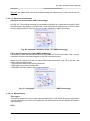
Once your instruments are connected, you can have all the details about the experiments that
are run and on which channels of which instruments they are run by accessing the Global
View.
There are several ways to access the Global View window:
1. It automatically appears once the User Name is set the first time EC-Lab is opened.
2. In the Devices box, click on
3. Press Ctrl+W
4. Go to View\Global View
9
EC-Lab Software User's Manual
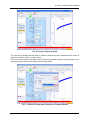
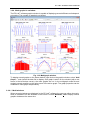
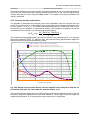
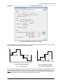
Fig. 3: “Global View” window.
The global view of the channels shows the following information:
 On the left the instruments to which the computer is connected. The active or selected
instrument will appear in a different color
 channel number with Z if impedance option is available on the channel. If the channels are
synchronized, grouped, or execute a stack, a bipotentiostat technique, they will appear in
a different color.
- A “l” letter is displayed near the channel number when a linear scan generator is added
to a channel board (for SP-300 technology).
- A ”s” letter is displayed in the left side of the channel column if a channel is synchronized
with other channel.
- A “g” letter is displayed in the left side of the channel column if a channel is grouped with
other channels.






an indicative ‘BAR’ in -white if there is no experiment running, colored if the channel is
running. If no pstat board, booster or low current board inserted in a slot, the corresponding
slot number is greyed out and no information is displayed on the global View window.
user - the channel is available (no username) or is (was) used by another user. Several
users can be connected to the instrument, each of the users having one or several channels.
status - the running sequence if an experiment is in progress: Oxidation, Reduction, or
either oxidation or reduction in impedance technique, Relax for open circuit potential,
Paused for a paused experiment and stopped for channel where an error happened.
tech. - the experiment type once loaded (e.g. CV for Cyclic Voltammetry, GCPL for Galvanostatic Cycling with Potential Limitation, PEIS for potentio impedance, etc...).
cable - only for SP-300, SP-200, SP-240 VSP-300 and VMP-300 - the type of cable connected to the board, standard if a standard cable is connected to the board. low current
if the Ultra-Low Current option is connected or straight if no cable is connected
amplifier - the booster type if connected: 1 A, 2 A, 4 A, 5 A, 8 A, 10 A, 20 A, 80 A, 100 A,
a 500 W, a 2 kW load or none (VMP2, VMP3 technology), 1 A/48 V, 2A/30V, 4A/14V and
10A/5V (for SP-300 technology). For VMP-3 technology a “Low current” is displayed as
amplifier type when the low current board is connected to a channel board.
The user has the ability to add several current variables on the global view such as “time, Ewe,
I, buffer, Temperature, control Ece, Ewe-Ece”. These variables can be chosen by right-clicking
anywhere on the Global View. Note that the displayed variables are the same for all the channels and all the instruments. Double-clicking on any of the channel window will replace the
global view by the specific view of the selected channel.
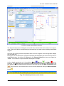
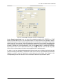
Double click on a channel of the global view to select it. You will get the following window:
10
EC-Lab Software User's Manual
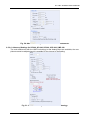
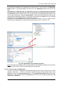
Fig. 4: Main window for experiment setting.
This window shows at the very top, in the blue title bar: the software version, the connected
instrument, the IP address (if connected through a LAN), the active channel, the name of the
experiment (i.e. name of the data file) and the selected technique (if any).
2.2 EC-Lab Main Menu
Fig. 5: The bar menu of EC-Lab software main window.
The Main Menu bar has been designed in such a way that it follows a progression from the
experiment definition to the curves analysis. Each menu is described below.
11
EC-Lab Software User's Manual
Fig. 8: View Menu.
Fig. 7: Edit Menu.
Fig. 6: Experiment Menu.
This menu allows the user to
build a new experiment and
load an existing setting file or
an existing data file made
with a Bio-Logic potentiostat
or another one. EC-Lab® is
able to read other manufacturer files formats. Saving
options are also available.
The second frame offers the
user the possibility to Export
as or Import from Text.
Experiment commands (Accept, Cancel Modify, Run,
Pause, Next Sequence and
Next Technique) are in the
third frame.
Print and Exit commands
can be found in the fourth
frame. The last opened files
are listed in the fourth frame.
12
The “Edit” menu can be used
to build an experiment, insert
(Move up or Move down), or
Remove a Technique from
an
experiment.
The
Group/Synchronize/Stack/Bipot window is
also available in this menu.
The second frame is for sequence addition or removal
from a technique (when this is
possible), and the two last
ones offer Copy options
(Graph, Data, ZSimpWin format) on the graphic window.
This menu is very useful as it allows the user to show the Global
View, a Graph Description of
the technique, to switch between
the Column/Flowchart view of
the settings.
The second frame shows the active channel and its status. The
third frame allows the user to
choose which Tool Bars to have
displayed or to show the Status
Bar or warning Messages.
EC-Lab Software User's Manual
Fig. 10: Analysis Menu
Fig. 11: Tools Menu.
Fig. 9: Graph Menu.
This menu includes all
the Graph tools (zoom in
and out, points selection,
auto scale, and Graph
Properties) and the
graph
representation
menu. This menu also allows the user to load or
add new files to the
graph. This menu is
equivalent to the RightClick menu on the Graph
window.
The Analysis menu contains
various Analysis tools, sorted
by themes: Math, General
Electrochemistry, EIS, Batteries,
Photovoltaic/Fuel
Cells, supercapacitors and
Corrosion. More details will be
given in Chapter 4.
The Tools menu is composed
of three frames. The first one
is for the data file modification
(Modify Cell Characteristics, Split File, Under Sampling).
The second frame is related to
operations performed on the
firmware (Channel Calibration, Repair Channel, Downgrade or Upgrade the Firmware) or the file (Repair File,
Batch mode).
The last frame gives access to
various tools such as Tera
Term Pro (used to change the
instrument
configuration),
Calculator and Notepad.
13
EC-Lab Software User's Manual
Fig. 13: Windows Menu.
Fig. 12: Config Menu.
Fig. 14: Help Menu.
The config menu is dedicated This menu is used to
to display username window, choose how to display the
to access and modify soft- windows and close them.
ware configuration, to access
virtual potentiostats. All the
functions here (except the
Options) are available from
the Devices or Experiments
boxes.
The Help menu contains pdf
files of the Software, the Instrument installation and
configuration Manuals and
several quickstarts This menu
provides also a direct link to
the Bio-Logic website and a
way to check for software Updates. It is also possible to
access to the Newsletter (automatically displayed when
the software is installed for
the first time on the computer
and for each upgrade).
2.3 Tool Bars
2.3.1 Main Tool Bar
Fig. 15: Main Tool Bar.
The user can change the buttons displayed in the tool bar. To do that, the user can either click
on Config\Options\Tool bars/menus\Main Tool Bar and select or deselect the desired buttons (see part 2.14.6, page 66 for more details) or right-click with the mouse on the Main Tool
Bar and choose Options.
14
EC-Lab Software User's Manual
Fig. 16: Main Tool Bar menu to choose the icons to be displayed.
2.3.2 Channel tool bar
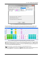
You can see below 16 buttons (depending on the instrument and on the number of channels
that can be inserted into the chassis). These buttons correspond to the actual slots. They are
not displayed if the slot is unused or if there is a booster board or low current board inserted in
it (Fig. 18). The channel number is always the slot number.
Fig. 17: Channel Selection Tool Bar of a multichannel fully loaded.
If no channel board inserted into a slot or if a booster, low current board inserted into a slot,
the corresponding slot is not displayed in the channel selection tool bar.
Fig. 18: Channel Selection Tool Bar of a multichannel partially loaded.
By clicking on the button, the user can select the current channel(s). Clicking on one of the
buttons enables the user to see the channel status. The corresponding bars give the on/off
status of the channels: white if there is no experiment running or colored if the channel is
running:
Yellow: charge mode
Green: discharge mode
Turquoise: OCV mode
Red: error mode
Pink: Impedance mode
Blue: Pause mode
White: stopped mode
15
EC-Lab Software User's Manual
2.3.3 Graph Tool Bar
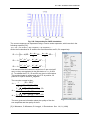
The Graph Tool Bar with shortcut buttons (including zoom, rescale, analyses, and graph properties) is attached to the graph. Report to the graphics tools part for more details
Fig. 19: Graph Tool Bar.
Also attached to the Graph window is the Fast Graph Selection Tool Bar that can be used to
rapidly plot certain variables and choose the cycles/loop to be displayed:
Fig. 20: Fast Graph Selection Tool Bar and cycle/loop filter.
2.3.4 Status Tool Bar
At the bottom of the main window, the Status Tool Bar can be seen
Fig. 21: Status Tool Bar for a VMP3.
The following informations are displayed:
- the connected device
- the instrument’s IP (internet protocol) address if the instrument is connected to the computer through an Ethernet connection or USB for an USB connection. For multichannel
potentiostat/galvanostat or for measurements that require a fast sampling rate the use of
the Ethernet connexion is strongly recommended.
- the selected channel,
- a lock showing the Modify/Accept mode: “Read mode” or “Modify mode”,
- the remote status (received or disconnected). For VMP2 and for SP-300 technology instrument "Warm up autocalibration" is displayed when the instrument perform an autocalibration (usually after connecting the instrument to EC-Lab®)
- the user name,
- the mouse coordinates on the graphic display,
- the data transfer rate in bit/s.
2.3.5 Current Values Tool Bar
On the left side or at the bottom, the Tool Bar with the Current Values can be seen.
Fig. 22: Current Values Tool Bar.






16
Status gives the nature of the running sequence: oxidation, reduction, relax (open circuit, measuring the potential), paused or stopped. Buffer full will be displayed in the case
where the instrument’s intermediate buffer is full (saturated network...),
Time, Ewe and Current are the time, the working electrode potential and the current from
the beginning of the experiment,
Buffer indicates the buffer filling level
Eoc is the potential value reached at the end of the previous open circuit period,
Q - Q0 is the total charge since the beginning of the experiment,
I range The current range,
EC-Lab Software User's Manual



I0 (or E0). I0 is the initial current value obtained just after a potential step in potentiodynamic
mode,
Ns is the number of the current sequence,
nc is the number of the current cycle or loop.
Note: Two protocols (Batteries: GCPL and PCGA) propose the additional variable X - X0, which
is the insertion rate.
This Tool Bar can be unlocked with the mouse and set as a linear bar locked to the status bar
at bottom of EC-Lab window or to the graphic bar at the top of the window.
Fig. 23: Current Values Tool Bar in a linear format.
Note: In the default configuration, all the tool bars are locked in their position. At the user’s
convenience, tool bars can be dragged to other places in the window. To do so, click on Config\Option\Tool bars/menus and deactivate the “Lock Tool bars” box. This will be effective
after restarting the software. Once the user has defined a new configuration of the tool bars,
the tool bar can be relocked the same way it was unlocked.
Note also that some of the current values can be displayed in bold using the Config\Option\Colors tab.
2.4 Devices box
As mentioned earlier, it is now possible with only one EC-Lab open session to be connected
to and control several instruments. In earlier versions of EC-Lab, it was necessary to open as
many EC-Lab sessions as the number of instruments.
The Multi-Connection is performed using the Devices box on the main window (See Fig. 4 and
23). The
and
buttons allow the user to add or remove instruments linked to the computer
either through USB or Ethernet. The
and
buttons are used to connect and disconnect,
respectively, an instrument to the computer. The
as described in the beginning of part 2.1. Finally, the
potentiostat (see part 2.13).
button is used to show the global view,
button is used to connect to a virtual
Fig. 24: Multi-device connection box
If more details are needed about the connection of the instrument, please refer to the corresponding “Installation and configuration manual”.
17
EC-Lab Software User's Manual
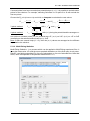
2.5 Experiments box
By default, the highlighted tab in the Experiments box is the “Parameters Settings” tab. Four
tabs allow the user to switch between three settings associated to the protocol: the "Advanced
Settings", the "Cell Characteristics", “External Device” and the "Parameters Settings".
2.5.1 Parameters Settings Tab
When no technique or application is loaded in the Experiments box, a small text is displayed
indicating how to proceed:
“No experiment loaded on current channel.
To create an experiment please selects one of the following actions:
New
Load Settings
New Stack (if connected to a multichannel)
Load Stack Settings (if connected to a multichannel)

The column will contain the techniques of a linked experiment. The settings of each
technique will be available by clicking on the icon of the technique.

The “Turn to OCV between techniques” option offers the possibility to add an OCV
period between linked techniques. This OCV period allows the instrument to change its current
ranging.
Fig. 25: Top row in the Parameters Settings window.
The button
is available to show the graph describing the technique and its variables.
2.5.1.1 Right-click on the “Parameters Settings” tab
EC-Lab software contains a context menu. Right-click on the main EC-Lab window to display
all the command available on the mouse right-click. Commands on the mouse right-click depend on the displayed window. Other commands are available with the mouse right-click on
the graphic display.
18
EC-Lab Software User's Manual
Fig. 26: Mouse right-click on the main window of EC-Lab software.
Most of the commands are available with the right-click. They are separated into 6 frames. The
first frame concerns the available setting tabs, the second one is for the experiment from building to printing. The third frame is for the modification of an experiment (actions on techniques)
and the creation of linked experiments. The fourth one is dedicated to sequences (addition,
removal) and the fifth one to the controls during the run. The sixth and seventh frames are
additional functions described above and the last frame is a direct access to the Options tab.
2.5.1.2 Selecting a technique
First select a channel on the channel bar. There are three different ways to load a new experiment.
1- Click on the “New Experiment” button
.
2- Click on the blue “New” link on the parameter settings window.
3- The user can also click on the right button of the mouse and select “New Experiment”
in the menu.
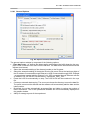
Note: - It is not always necessary to click on the “Modify” button before selecting a command.
The software is able to switch to the “Modify” mode when the user wants to change the settings
parameters. In that case the following message is displayed:
19
EC-Lab Software User's Manual
Fig. 27: Message displayed before switching to Modify mode.
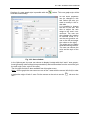
Click on Yes and the “Insert Techniques” window will appear with the different techniques
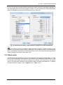
available with EC-Lab software.
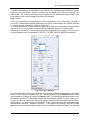
Fig. 28: Techniques selection window.
The techniques available with EC-Lab software are divided in two different sections: Electrochemical Techniques and Electrochemical Applications.
Electrochemical Techniques folder includes voltamperometric techniques, electrochemical impedance spectroscopy, pulsed techniques, a tool to build complex experiments, manual control, ohmic drop determination techniques and also Bipotentiostat techniques for multichannel
instruments. Electrochemical Applications folder includes battery testing, supercapacitor, photovoltaic/fuel cell testing, corrosion measurements, custom applications and special applications.
At the bottom of this window different options can be selected when a protocol is loaded. In
the case of linked techniques, the user can insert the technique either before or after the technique already loaded in the Experiments Box. This option will be described in detail in the
Linked Techniques section (part 2.7). The technique can be loaded with or without the “Cell
Characteristics” and the “Advanced Settings” of the default setting file. The experiment can be
saved as a custom application (see Custom Applications section (in the Techniques and
Applications manual).
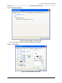
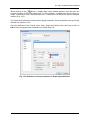
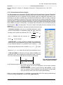
For example, choose the cyclic voltammetry technique and click OK or double click. On the
right frame, a picture and description is available for each protocol.
20
EC-Lab Software User's Manual
Fig. 29: CV technique picture and description on the experiment window.
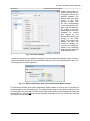
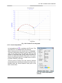
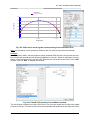
2.5.1.3 Changing the parameters of a technique
When a technique is selected the default open window is the "Parameters Settings" window.
The user must type the experiment parameters into the boxes of the blocks. Two ways are
available to display a technique: either the detailed flow diagram (Fig. 30) and its table, or the
detailed column diagram (Fig. 31).
It is possible to switch between the two modes of display using the
button. Setting parameters can also be done using selected settings files from user’s previous experiment files.
Click on the Load Settings icon
then select an .mps setting file or a previous .mpr raw
file corresponding to the selected technique and click OK. You can right-click on the mouse
and select “Load settings…”.
Note: Most of the techniques allow the user to add sequences of the same techniques using
mouse right-click or using the Edit menu. On the "Parameters Settings" tab, the CV detailed
flow diagram or the column diagram is displayed:
21
EC-Lab Software User's Manual
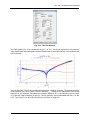
Fig. 30: Cyclic Voltammetry detailed flow diagram.
Fig. 31: Cyclic Voltammetry detailed column diagram.
22
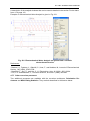
EC-Lab Software User's Manual
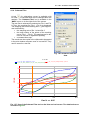
When a technique is loaded on a channel, the detailed column diagram is displayed. On top
of the diagram, the Turn to OCV option can be seen as well as the button
show the graph describing the technique and its variables (cf. Fig.32).
, available to
Fig. 32: CV graphic description.
The EC-Lab software protocols are made of blocks. Each block is dedicated to a particular
function. A block in grey color means it is not active. The user has to set parameters in the
boxes to activate a block, which becomes colored.
When available, the recording function "Record" can be used with either dER or dtR resolution
or with both. Data recording with dER resolution reduces the number of experimental points
without losing any relevant changes in potential. If there is no potential change, only points
according to the dtR value are recorded. If there is a steep change in potential, the recording
rate increases according to dER.
In every technique with potential control and current measurement, the user can choose the
current recording conditions between an averaged value (per potential step for a sweep) and
an instantaneous value every dt (see the Techniques and Applications manual).
When a technique is loaded in the parameters settings window, a small icon is displayed on
the left of the flow diagram with the name of the technique and its number (rank) in the experiment (in case of linked techniques). During a run, the technique that is being performed is
indicated by a black arrow.
Notes:
- E Range adjustment
On the technique the user can define the potential range (min and max values) to improve the
potential resolution from 305 µV (333 µV for SP-300 technology instruments) down to 5 µV for
VMP3 technology instruments (down to 1µV for SP-300 technology instruments).
- Scan rate setting
When entering the potential scan rate in mV/s the default choice of the system proposes a
scan rate, as close as possible to the requested one and obtained with the smallest possible
step amplitude. The scan rate is defined by dE/dt.
- I Range
The current range has to be fixed by the user. When the current is a measured value, I measured can be greater than the chosen I Range without "current overflow" error message. In this
case the potential range is reduced to ± 9 V instead of ± 10 V. The maximum measurable
current is 2.4*I Range. For example with I Range = 10 mA, the current measured can be 24 mA
with a potential range ± 9 V. The same thing is possible when the current is controlled (For
more details about that, please see section 6.3).
23
EC-Lab Software User's Manual
With booster ranges and 1 A range of VMP-300, VSP-300, SP-240, SP-300 and SP-200, this
relationship is not valid.
- Bandwidth
The VMP2/Z, VMP3, VSP, MPG2-XXX series, SP-50, SP-150, HCP-803 and HCP-1005 devices propose a choice of 7 bandwidths (''damping factors''), and 9 for SP-300, SP-200, SP240 VSP-300 and VMP-300 devices in the regulation loop of the potentiostat. The frequency
bandwidth depends on the cell impedance and the user should test filtering effect on his experiment before choosing the damping factor.
The following table gives typical frequency bandwidths of the control amplifiers poles for the
VMP3, VSP, MPG2, SP-50, SP-150, HCP-803 and VMP2:
Bandwidth
Frequency
7
680 kHz
6
217 kHz
5
62 kHz
4
21 kHz
3
3.2 kHz
2
318 Hz
1
32 Hz
Note: For more details about bandwidth definition for the SP-300, SP-200/SP-240, VSP-300,
VMP-300 instruments, refer to the installation and configuration manual for VMP-300 based
instruments.
When the mouse pointer stays for several seconds on a box a
hint appears. The hint is a visual control text that gives the user
information about the box. It shows the min and the max values
of the variable as well as the value that cancels the box i.e. the
value for which the box will be skipped.
Fig. 33: Hint.
- Sequences within a technique.
If the user wants to perform an experiment composed of the same technique but with different
parameters, the sequences can be used. These sequences are accessible in two different
ways depending on the type of diagram used.
Column Mode
Below the “Turn to OCV” line, “+” and “-“ buttons can be seen (Fig. 34).
Fig. 34 : The “+” and “-“ buttons to add sequences.
Clicking on the “+” button will add a sequence with the same parameters as the previous sequence. Clicking on the “-“ sequence will remove the sequence. Up to 99 sequences can be
added. Note that only one data file will be created and that you can only add sequences of the
same technique.
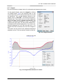
Flow Chart Mode
24
EC-Lab Software User's Manual
In the flow diagram mode, a table appears automatically. One row of the table is a sequence
of the experiment. The experiment parameters can be reached and modified in the table cells
as well as in the flow diagram of the parameter settings window
Fig. 35: EC-Lab table (shown in Flow Chart mode).
During the run, the active row of the table (running sequence) is highlighted. The default number of rows is 30. The user can insert, delete, append, copy, and paste up to 99 rows by clicking
the right button of the mouse. It can be a very interesting tool when the user wants to repeat
an experiment with one different parameter in a sequence. It is also possible to cut, copy and
paste only one cell of the table.
Note:
- The user can define different current ranges for each sequence if an OCV period separates the sequences (at the beginning of each sequence for example).
- It is possible to repeat a block in a sequence (go to sequence Ns’).
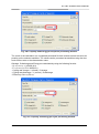
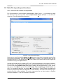
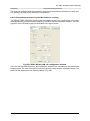
2.5.2 Cell Characteristics Tab
Clicking on the "Cell Characteristics" tab will display the cell characteristics window. This
window is composed of three blocks: Cell Description, Reference Electrode and Record.
Please see below:
Fig. 36: Cell Characteristics tab (standard connection with VMP3 technology).
25
EC-Lab Software User's Manual
2.5.2.1 Cell Description
This window has a standard configuration and the “battery” configuration can be activated by
clicking on the “Battery” button.
2.5.2.1.1 Standard “Cell Description” frame
Fig. 37: Standard Cell Description frame.
You can either fill the blank boxes manually, entering comments and values, or load them from
a .mps setting file or a .mpr raw file using Load Settings... on the right-click menu. This window allows the user to:
 add information about the electrochemical cell (material, initial state, electrolyte and comments)
 set the electrode surface area, the characteristic mass, the equivalent weight and the density of the studied material.
- The surface area is the area of the sample used as a working electrode and exposed to the electrolyte. :
- The characteristic mass is needed if the user needs to express any variable per
unit of mass. It can be the mass of a whole battery or the mass of a sample.
- The equivalent weight is the characteristic mass divided by the number of electrons
exchanged during the electrochemical reaction, in most cases the dissolution of the
metal.
Once defined, these parameters are automatically used to calculate, for example, the corrosion
rate after a Tafel Fit or display the current as a current density. It is also possible to modify the
electrode surface area or characteristic mass after the experiment by selecting “Edit surface
and mass” in the Graph Tool Bar. The window below appears
Fig. 38: Edit surface and mass window.
26
EC-Lab Software User's Manual
Another way is to use the Modify Cell Characteristics in the Tools tab of the main tool bar. (see
2.2.2.1)
2.5.2.1.2 Battery “Cell Description” frame
When the “Battery” button is pressed, additional parameters related to batteries show up. Note
that these parameters are automatically displayed when a battery testing setting file is loaded.
The corresponding window is as follows:
Fig. 39: Cell description window for a battery experiment or
when the battery button is pressed.
In addition to the parameters described above, this window allows the user to enter the physical characteristics corresponding to the intercalation material. This makes on-line monitoring
of the redox processes possible in terms of normalized units.
Let us review all the parameters:
 The mass of active material in the cell has to be set with a given insertion coefficient
xmass in the compound of interest (for example xmass = 1 for LiCoO2). These two
parameters mass and xmass are actually related to the battery itself. This mass is different from the characteristic mass. It is only used to calculate the insertion rate x and
not the massic variables: (I, Q, P, C, Energy)/unit of mass
 The molecular weight of the active material is the molecular weight of the active material substracted by the atomic weight of the intercalated ion. The atomic weight of the
intercalated ion is set in a separate box. For example, for LiCoO2, the molecular weight
27
EC-Lab Software User's Manual


of CoO2 is 90.93 g.mol-1 and the atomic weight of the intercalated Lithium Li+ is 6.94
g.mol-1.
The initial insertion rate xo.
ne is the number of electrons transferred per mole of intercalated ion.
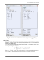
An intermediate variable Xf is calculated using the following formula:
Mass is in mg,
Molecular weight and the atomic weight are in g/mol, this is why mass needs to be multiplied
by 0.001,
F is equal to 26801 mA.h/mol.
Xf quantifies the change of insertion coefficient of the considered ion when a charge of 1 mA.h
is passed through the cell (or disintercalated when a discharge of -1 mA.h is passed). The
charge needed to increase Xf of 1 is given in the window:
“for x=1, Q= 26802 mA.h”.
The variable x, which is the insertion coefficient of the inserted ion (or stoichiometry of the
inserted ion in the concerned compound) resulting from the charge, is calculated using the
following formula:
x = xo + Xf (Q-Qo)
x is the sum of xo the initial insertion coefficient and Xf the change of insertion coefficient during
the charge (or disintercalated during the discharge) Q-Qo.
Qo is the initial state of charge of the battery and is calculated using xo.
Finally, it is possible to enter the capacity C of the battery in A.h or mA.h. The capacity of the
battery is the total charge that can be passed in the battery. A capacity of 3.2 A.h means that
the fully charged battery will be totally discharged if a current of -3.2 A is applied during 1 hour.
In the techniques dedicated to batteries and especially the GCPL techniques and Modulo Bat
technique (MB), it is possible to define the charge or discharge current as a function of the
capacity. For instance, using a battery of 3.2 A.h, if the charge is set at C/2, it means that the
battery will be charged with a current of 1.6 A. The time of the charge is defined elsewhere in
the technique (see “EC-Lab Software Techniques and Applications”).
2.5.2.2 Reference electrode
It is possible to set the reference electrode used in the experiment (either chosen in the list or
added while clicking on the corresponding tab). The common reference electrodes are available. If “unspecified” is entered, then the potential will be given in absolute value. Note that it is
possible to add a custom reference electrode and that the Reference electrode menu is also
available in Config\Options\Reference.
Fig. 40: The Reference electrode block
28
EC-Lab Software User's Manual
2.5.2.3 Record
Fig. 41: The Record block.
In addition to the variables recorded by default (mainly Ewe (= Ref1-Ref2 or S1-S2), I and other
variables depending on the chosen techniques), the user can choose to record:
 the counter electrode potential (Ece = Ref3-Ref2 or S3-S2)
 the power P = Ewe*I computed by the hardware
 analog external signals (pH, T, P,...) using auxiliary inputs 1 (Analog In1) and 2 (Analog
In2). These signals must be configured using the window opened by clicking on the link
in blue.
It must be noted that Ewe, Ece and the power P are hardware variables and are directly coming
from the potentiostat board. If the user does not choose to record P, it will nonetheless appear
as a default variable but will be calculated not by the potentiostat but by the software using the
I and Ewe values stored in the data file by the software.
The hardware P is generally more accurate. The variable Ewe - Ece is calculated by the software.
Except MPG2, there is no Ece variable with MG-2XX series instruments
The Record block gives also the possibility to see the properties of the data file in which the
variables will be stored. All boxes (Acquisition started on, host, directory and file) are filled
automatically when the experiment is started.
Fig. 42: Cell characteristics Files window.
2.5.3 Advanced Settings tab
The advanced settings window includes different hardware and software parameters that depend on the type of instrument. To change the values, click on the Modify button, enter the
new settings, and click on the Accept button to send the new settings to the instrument. Note:
the “Advanced Settings” window is available for all the protocols.
29
EC-Lab Software User's Manual
2.5.3.1 Advanced Settings with VMP3, VSP, SP-50, SP-150
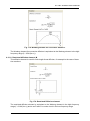
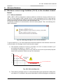
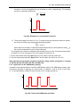
The advanced settings window includes several hardware parameters and software parameters divided in four blocks: Compliance, Safety Limits, Electrode Connections, and Miscellaneous (Cf Fig. 43). Note that for SP-50 the compliance is not adjustable [-10V,+10V].
Fig. 43: Advanced Settings window for VMP3, VSP, SP-50, SP-150 instruments.
2.5.3.1.1 Compliance
The compliance corresponds to the potential range of the Counter Electrode versus the Working Electrode potential (|Ewe-Ece|). This option has to be modified only for electrochemical cells
with more than 10 V potential difference between the counter and the working electrode. One
can change the instrument compliance voltage between the CE and the WE electrodes from
– 20 V  0 V to 0 V  20 V, by steps of 1 V. In all the ranges the control and measurement
30
EC-Lab Software User's Manual
of the variables are available. Note that for SP-50 the adjustable compliance is not available.
REF
The default compliance of CE vs. WE is
± 10 V. For example, while working with a
12 V battery, with the CE electrode connected to the minus and the WE connected
to the plus, the potential of CE vs. WE will be
– 12 V. That is not in the default compliance.
In order to have the CE potential in the right
compliance, set the CE vs. WE compliance
from – 15 V to + 5 V.
When the working electrode is connected to
the minus and the counter electrode to the
plus, the potential of CE versus WE will be
+ 12 V. Then the compliance must be shifted
between – 5 and + 15 V.
Fig. 44: 12 V battery, WE on +.
WE
CE REF
Fig. 45: 12 V battery, WE on -.
Warning: the compliance must be properly set before connecting the cells to avoid cell disturbance.
2.5.3.1.2 Safety Limits
Most of protocols already have potential, current or charge limits (for example Galvanostatic
Cycling with Potential Limitation (GCPL): limit Ewe to EM and |Q| to QM, ...) that are used to
make decision (in general, the next step) during the experiment run.
The experiment limits have been designed to enter higher limits than the limits set into the
protocols to prevent cells from being damaged. Once an experiment limit is reached, the experiment is paused. Then the user can correct the settings and continue the run with the Resume button or stop the experiment.
To select an experiment limit, check the limit and enter a value and a time, for example:
Ewe max = 5 V, for t > 100 ms. Then the limit will be reached if Ewe is greater than 5 V during a
time longer than 100 ms. Once selected, an experiment limit is active during the whole experiment run.
It is also possible to set an upper or higher limit on the external analog signals Analog IN1 or
Analog IN2.
“E stack slave min” allows the user to set a lower limit that will be applied on each individual
element (“slave”) of a stack of batteries. This ensures that no battery is damaged during the
experiment.
“E stack slave max” allows the user to set an upper limit that will be applied on each individual
element (“slave”) of a stack of batteries. This ensures that no battery is damaged during the
experiment.
“Do not start on E overload” allows the user to not start an experiment in case of an overload
of the potential E. It allows also the stop of an experiment in case of a potential overload.
31
EC-Lab Software User's Manual
Warning: the safety limits cannot be modified during the experiment run and must be set before.
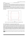
2.5.3.1.3 Electrode Connections
Standard connection mode (VMP3 technology)
See Fig. 42: The working electrode is connected to CA2/Ref1, the reference electrode to Ref2
and the counter electrode to CA1/Ref3. Ref1, Ref2, Ref3 (Ref for reference) are used to measure the voltage and CA2 and CA1 (CA for Current Amplifier) to apply the current.
Fig. 46: Standard connection mode ( for VMP3 technology).
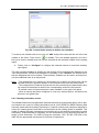
CE to Ground connection mode (VMP3 technology)
It is possible to work with several WE (several RE) and one CE in the same bath. Then, counter
electrodes must be connected together to the Ref1 lead and ground.
Disconnect the cables from the cell, select “Electrode connections” and “CE to ground” and
reconnect the cell as follows:
- CA1 and Ref3 leads to the working electrode
- Ref2 lead to the reference electrode
- GROUND and Ref1 leads to the counter electrode
Fig. 47: Configuration CE to ground (N’Stat) for VMP3 technology
2.5.3.1.4 Miscellaneous
Text export
This option allows the user to export data automatically in text format during the experiment
(on-line exportation). A new file is created with the same name as the raw data file but with an
.mpt extension.
Filter
32
EC-Lab Software User's Manual
This option allows the user to filter by the mean of the software the data just after the run by
ticking this box before running the experiment. A new file is created with the same name as
the raw data file but with an .mpp extension. This Filter tool is described in the paragraph
dedicated to Analysis tools.
Fig. 48: Filter window.
Smooth (with sliding average)
For all the protocols, the user can smooth all values (I, Ewe, Ece, Aux1…) with a sliding average.
To proceed, check smooth and enter the smooth window size (between 2 and 100 points).
Create one data file per loop
This option offers the possibility to create one data file per loop for each technique of a linked
experiment. Then the data files will have a prefix number to define the order in the experiment.
For example, an experiment is composed of OCV, CA and then a Loop on the OCV for 9 times.
If the “Create one data file per loop” box is not ticked, the data from the experiment will be
stored in two .mpr files: one for the OCV and one for the CA.
If the “Create one data file per loop” is ticked, then the data from the experiment will be stored
in twenty .mpr files: one for each OCV and CA of each loop.
2.5.3.2 Advanced Settings with HCP-803, HCP-1005, CLB-500 and CLB-2000
For HCP-1005, HCP-803 and CLB-500, the compliance value and the electrode connection
are fixed. The other limits and functions are the same as in 2.5.3.1.
33
EC-Lab Software User's Manual
Fig. 49: Advanced settings window for HCP-803, HCP-1005, CLB-500 and CLB-2000 instrument.
2.5.3.3 Advanced Settings with MPG-2XX
It is the same window as Fig. 49 except that the electrode connections are not displayed as
only one connection is available with MPG-2XX (CE-to ground connection).
34
EC-Lab Software User's Manual
Fig. 50: Advanced settings window for MPG-2XX instruments.
2.5.3.4 Advanced Settings for SP-200, SP-240, SP-300, VSP-300, VMP-300
The main differences with the VMP3 technology is that Analog filters are available, the compliance cannot be adjusted and it is possible for the channel to be floating.
Fig. 51: Advanced settings window for SP-300 technology.
35
EC-Lab Software User's Manual
For SP-200, SP-240, SP-300, VSP-300 and VMP-300 instruments, the compliance is not adjustable and is equal to +/- 12 V. However for the booster belonging to the SP-300 technology,
the compliance depends on the booster type. For these boosters the compliance is as follows:
+/- 49 V for the 1A/48V, +/-30V for the 2A/30V, [-3, +14V] for the 4A/14V and [0,5V] for the
10A/5V booster.
2.5.3.4.1 Filtering
This option is only available for the SP-300 technology. It is possible to filter potential (E) and
current (I) by hardware. Three analog filters exist: 5 Hz, 1 kHz and 50 kHz. It is also possible
to obtain the raw data by selecting No filter (None).
2.5.3.4.2 Channel
This menu is only available for the SP-300 technology. The Channel menu allows the user to
select between Grounded and Floating mode for the used channel. The Floating mode must
be used when the potentiostat is connected to a grounded cell (e.g. autoclave, pipeline etc…).
The potentiostat needs to be floating to prevent current from looping in the cell.
2.5.3.4.3 Ultra Low Current Option
This option is only available with the SP-300 technology when the Ultra-Low Current option is
connected to the channel. This option is necessary when low current ability at relatively high
speed is required. What is considered a high speed depends on the magnitude of the measured current. Lower is the current lower is the high speed. Ticking “High Speed Scan” helps
compensate the bias current (typically 300 fA), which can become not negligible anymore at
low currents (typically <1 nA). In these extreme conditions, measurements can appear distorted. For instance, a loop can show up at the vertex (Fig. 52) as a result of an asynchronicity
of the measured potential and measured current.
The value of current scan for which the correction must be applied also depends on the intrinsic
characteristics of the cell (type of electrode, distance between electrodes, ...). The correction
offered in the “Advanced Settings” window is automatically selected when Ultra Low Current
Option is connected.
36
EC-Lab Software User's Manual
Note that if the High Speed Scan box is ticked, the data may be noisier especially for ranges
below 1 nA (Fig. 53). It is possible to reduce the noise by numerically filtering the data after
their acquisition (the numerical filtering is available in the “Math” menu of the “Analysis” tab).
<I> vs . Ew e
UME_5V s_sans compensation_1nA .mpr, cycle 3 #
UME_5V s_avec compensation_1nA .mpr, cycle 3
2
1.5
<I> vs . Ew e
UME_5V s_sans compensation_1nA .mpr, cycle 3 #
UME_5V s_avec compensation_1nA .mpr, cycle 3
1
2.25
0
<I>/nA
2.2
-0.5
2.15
2.1
-1
2.05
-1.5
2
-2
0.38
0
0.2
0.39
0.4
Ewe/V vs. SCE
0.4
Ewe/V vs. SCE
Fig. 52: CV carried out with an Ultra Microelectrode of 10 µm in a solution of ferrocene
in EtOH with TBAP as a supporting salt. The range of current is 1 nA and scan rate is
5 V.s-1. Zoom at the vertex. Blue line: no compensation, Red line: High Speed Scan compensation.
<I> vs . Ew e
CV _THF_Fc_1V s_100pA _avec toutes corrections.mpr, cycle 3
CV _THF_Fc_1V s_100pA _sans correction.mpr, cycle 2 #
150
100
<I>/pA
<I>/nA
2.3
0.5
50
0
-50
-100
0
0.5
Ewe/V
Fig. 53: CV carried out with Ultra Microelectrode of 10 µm in a solution of ferrocene in
THF without any supporting salt. The range of current is 100 pA and scan rate is 1 V.s-1.
Blue line: no compensation, Red line: High Speed Scan compensation.
37
EC-Lab Software User's Manual
2.5.3.4.4 Electrode Connections
Standard connection
See Fig. 49: The working electrode is connected to P1/S1, the reference electrode to S2 and
the counter electrode to P2/S3. S1, S2, S3 (S for Sense) are used to measure the voltage and
P1 and P2 (P for Power) to apply and measure the current. To set the standard connection,
proceed in the same way: disconnect first S1, S2 and S3 from the cell, and only after
disconnect P1 and P2, select Electrode connections = standard and set the next connections:
- P1 and S1 leads to the working electrode,
- S2 lead to the reference electrode,
- S3 and P2 leads to the counter electrode.
Then click on Apply configuration button.
CE to ground
See Fig. 52: Disconnect the cables from the cell, select
Electrode connections = CE to ground and reconnect the
cell as follows:
- P1 and S1 leads to the working electrode
- S2 lead to the reference electrode
- GROUND and S3 lead to the counter electrode
Fig. 54: Configuration CE to
ground (N’Stat) for SP-300
technology.
WE to ground connection mode
In addition to the CE to ground mode, a “WE to ground” connection mode is available with the
SP-200, SP-300, VSP-300 and VMP-300.
Fig. 55: WE to ground connetion for SP-300 technology.
This configuration is very useful for hydrogen permeation measurements where one working
electrode is grounded and connected to two different couples of counter electrode and reference electrode.
Refer to the “Installation and configuration manual” of the corresponding instruments for
more details on the CE to ground connection.
38
EC-Lab Software User's Manual
Warning: it is important to disconnect the electrodes from the cell, before changing the electrode connection, because of the difference between the leads assignment, the OCV may not
be properly applied.
Note: with CE to ground connection, CE vs. WE compliance is set to  12 V.
The CE to ground option is not available with the ZRA protocol (Zero Resistance Ammeter).
+/- 48 V control mode
This connexion mode is available with the SP-300/VSP-300/VMP-300 when a 1 A/48 V booster
connected to the standard channel board.
Disconnect the cables from the cell, select Electrode
connections = +/- 48 V control and reconnect the cell as
follows:
- P2 and S3 lead to the working electrode
- S2 leads to the reference electrode
- P1 and S1 lead to the counter electrode
Fig. 56: +/- 48 V control mode
for SP-300 technology.
Refer to the “Installation and configuration manual” of your instrument for more details on the
+/- 48 V control connection mode.
+/- 30 V control mode
This connexion mode is available with the SP-300/VSP-300/VMP-300 when a 2A/30 V booster
connected to the standard channel board.
Disconnect the cables from the cell, select Electrode
connections = +/- 30 V control and reconnect the cell as
follows:
- P2 and S3 lead to the working electrode
- S2 leads to the reference electrode
- P1 and S1 lead to the counter electrode
Fig. 57: +/- 30 V control mode
for SP-300 technology.
Refer to the “Installation and configuration manual” of your instrument for more details on the
+/- 30 V control connection mode.
-3V;+14V control mode
The +14V;-3V is two-electrodes connexion mode available with the SP-240 and with SP300/VSP-300/VMP-300 when a 4A/14 V booster connected to the standard channel board.
39
EC-Lab Software User's Manual
Disconnect the cables from the cell, select Electrode
connections = -3V,+14 V control and reconnect the cell
as follows:
- P1, S1 and S2 leads to the working electrode
- S3 and P2 leads to the counter electrode
P.S: The impedance techniques are not available with 3V;+14V control mode.
Fig. 58:-3V;+14V control mode
for SP-300 technology.
2.6 Accepting and saving settings and running a technique
2.6.1 Accepting and saving settings
Once you have set the parameters of your experiment, click on the Accept icon
. It validates the Parameters Settings, the Cell Characteristics and the Advanced Settings and
sends them to the instrument. If the option is activated in the Config\option\Warning menu,
the following window will appear before accepting the settings:
Fig. 59: Summary window before accepting settings (VMP3 technology).
This window summarizes several parameters of the experiment. Click on Yes to accept the
settings and start the experiment. The settings can be set as default settings for the current
technique. Right-click on the mouse and select “Set settings as Default”. The parameter settings can be saved as an *.mps file in Experiment\save as\ or right-click on Save Experiment…, or click on
.
2.6.2 Running an experiment
Click on the Run button
40
. A filename selection window will appear:
EC-Lab Software User's Manual
Fig. 60: Filename selection window.
The default folder to save the data is called “Data”. The user can choose and create another
folder to save his data files. Type the filename.
Note: the filenames can be forced to end with the channel number using the Config\Option\General. This option is always fixed for grouped channels.
Clicking Save or pressing <ENTER> will start the experiment, and the Run button turns into
the Stop button.
One file is created when running the experiment: a binary raw data file, with an .mpr extension
automatically added that contains all the information for the experiment usually contained in
the Log file (the selected protocol, initial settings, instrument IP and channel N°, files director.).
The user can choose to separately save the Log file using the Config\Options\General menu.
2.7 Linking techniques
2.7.1 Description and settings
It is possible to link different protocols within the same run. This allows the user to create and
build complex experiments composed of up to 20 techniques. When created, the linked experiment settings can be saved either as an .mps file or as a “Custom Application”. In the first
case the settings can be loaded from the initial folder, and in the second case they appear in
the applications and can be reloaded whenever necessary.
Linked experiments can be made using the “Technique Builder” in the technique window.
The WAIT and LOOP options have been designed especially for linked experiments. Building
linked experiments is very easy with settings on the right-click menu. When the user rightclicks on the parameter settings window, the following menu pops up:
41
EC-Lab Software User's Manual
Fig. 61: Mouse right-click with the insert and remove options.
The second frame is especially dedicated to linked experiments. The “Insert New Technique”
function opens the technique selection window and can insert a new technique into the experiment. The additional technique can be added before or after the activated/selected technique
using the Insert Technique frame at the bottom left corner of the technique selection window:
Fig. 62: Insert before/after option of the technique selection window.
If the technique is not in the correct position in the series of experiments, the user can easily
move it up or down using the “Move Technique Before” and “Move Technique After” options
respectively.
Note: it is possible with the protocol linker to apply 50 ms OCV period between two protocols
(reduced to 0.6 ms if the previous protocol is an OCV). The user has just to activate "Turn to
OCV between techniques" in the Advanced Settings window. If this option is not selected
the user will not have the ability to select different current ranges for each linked technique.
When inserting a technique, other options are available:
Fig. 63: Loading options of the technique selection window.
If the boxes are checked it means that the default advanced settings, cell characteristics and
external devices settings will be associated with the inserted technique, regardless of any
change that was made.
Note that the Advanced Settings, Cell Characteristics and External devices are the same for
all the linked techniques.
If these boxes are unchecked, it means that the parameters set in the existing techniques will
be kept.
42
EC-Lab Software User's Manual
This option is useful if you need very specific parameters that you do not want to be erased
and replaced by the default parameters.
Note that more than one loop can be added to a linked experiment.
When the user clicks the Run button, the program asks for a file name that will be used for all
the linked experiments with the following rules:
experiment file name = user file name + "_" + experiment number + "_" + experiment
(short) name + "_" + "channel number" + ".mpr"
For example: the file name "MyFileName", will be used to generate these files:
Experiment 1: no file name for the Trigger In option
Experiment 2: MyFileName_2_MP_01.mpr
Experiment 3: MyFileName_3_WAIT_01.mpr
Experiment 4: no file name for the protocol linker loop
Each of these files will store the corresponding data points for all the loops.
Note:
1- It is possible to synchronize linked experiments on several channels.
2- One data file can be created per technique and per loop in a linked technique. In the
“Advanced settings” window, tick the box corresponding to “Create one data file per
loop”. The file name is created as follows:
“Filename” + _ + “technique number in link” + _ “technique name” + _
+ “channel number” + _ + “loop#”.mpr”
2.7.2 Applications
2.7.2.1 Linked experiments with EIS techniques
The following experiment is given as an example of linked experiment. This experiment is
composed of OCV, CA, CV, PEIS and Loop techniques.
43
EC-Lab Software User's Manual
Fig. 64: Linked experiments window.
The linked techniques are displayed on the left of the window with their number in the experiment. Click on the button corresponding to the technique you want to see to display the detailed
diagram.
Once the file name typed the acquisition starts, and the program shows the graphic display
with the data files.
During the run the technique in progress can easily be identified by an arrow next to the corresponding button. Its number is displayed in the Channel Values box (see next figure) as
“Tech”. The number of loops executed is displayed as “Loop”.
As for a single experiment run, it is possible to Pause /Resume
and Stop
the experiment. The Stop button will terminate the whole experiments acquisition. Nevertheless, one
can stop the current experiment and continue to the next one with the Next Technique button
in the tool bar. One can also move on to the next sequence using the Next Sequence
button
.
Fig. 65: Linked experiment current values.
44
EC-Lab Software User's Manual
Notes:
 The bipotentiostat techniques and the manual controls cannot be linked to any other
technique.
 The Polarization Resistance process calculation can be performed on the protocol
linker loops separately.
Linked experiments settings can be saved with Experiment, Save As, or on the right-click
menu with Save experiment… and reloaded with Experiment, Load settings... or with the
right-click menu Load settings....
Linked experiments settings files are text files with the *.mps extension like the standard settings files.
Please be aware that the recording of auxiliary signals from Analog In1 or Analog In2, and
power are disabled with an impedance technique. No external data points will be recorded
during the EIS measurement period. If the user accepts such settings, the following warning
message appears:
Fig. 66: Warning message on external signals recorded with EIS techniques
2.7.2.2 Application of linked experiments with ohmic drop compensation
The following experiment is given as an example of linked techniques but also to show how to
use the Ohmic drop compensation techniques. This experiment is composed of CA, CV, PEIS
and Loop techniques. This series of linked techniques illustrates the effect of the ohmic drop
compensation. Indeed, to compensate the ohmic drop during an experiment, the ZIR technique
has to be set before the techniques for which the compensation is done. To illustrate this the
Fig. 67 is given as an example. In the left side of the figure, the series PEIS + CV + ZIR + CV
is defined. On the right side of the figure, the second graph shows the superimposition of two
CV graphs: one compensated and one uncompensated.
45
EC-Lab Software User's Manual
Fig. 67: Linked experiments example with ohmic drop compensation technique.
2.8 Available commands during the run
During the experiment several commands remain active. Most of the settings can be changed
while the experiment is running. These changes appear in the log file.
2.8.1 Stop and Pause
Clicking on the Stop button
will display a message asking for confirmation. Clicking OK
stops the measurement. At that time a binary version of the .mpl file is appended to the .mpr
file. A raw data file .mpr is then obtained, which contains all the information on the experiment,
while the .mpl file is erased. The Log file can be kept as a separate file by checking the corresponding in Config\Options.
Clicking on the Pause button
will lead to a pause in the progress of the protocol and in the
measurement recordings. The cell will be disconnected from the current generator (but not
from the potential measurements). Then the Pause button switches to the Resume button
and clicking on this button continues the experiment (with a gap corresponding to the
pause time).
2.8.2 Next Technique/Next Sequence
It is possible during an experiment to move on to the Next Technique using the
or to the Next Sequence using the
46
button.
button
EC-Lab Software User's Manual
2.8.3 Modifying an experiment in progress
The Modify button
experiment is running.
enables the user to modify most of the parameter settings while the
The new set of parameters is sent to the instrument when clicking on the Accept button
.
It is taken into account within 200 µs for instruments of the VMP3 family and VMP-300 family.
All information on the change, the time it was done, the new settings etc., is appended to the
Log file (see section 3.2.6, page 83). Note that a warning message could appear before accepting the modification if this option is selected in Config\Option\Warning. Among all the
parameters, some of them cannot be modified on the fly such as I range E range and Bandwidth.
2.8.4 Repair channel
This tool allows a user to repair a channel board.
To have repair channel window, click on Tools menu and then repair channel windows.
The window below will be open.
The window contains four blocks:
1-Channel
2-Data buffer
3-Change saved file name
4-Reset
Fig. 68: Repair channel window
First block:
Selection of the channel the user wants to repair. The user should not modify the connection
mode (Ethernet or USB). In case of a multichannel instrument, it is recommended to select the
channel to repair and then select the same channel number in the repair channel window.
47
EC-Lab Software User's Manual
Second block:
This block allows user to lock the data transfer of the selected channel.
In the case of a multichannel, because of a wrong recording parameter (most of time dE or dI)
on one channel, many data points may be recorded and fill the buffer of the com board. The
data transfer procedure is stuck to this specific channel and is much slower for the other channel of the instrument. This tool allows user to block the data transfer of this channel, the data
point of the other channel will be retrieved.
Third block:
Allows the user to create a new file to store the coming data point.
It is useful for example when the user moves an experiment file during the experiment. In that
case, the user will have one file for the first part of the experiment and another one for data
point which are not yet transferred to the PC (after the creation of the new file).
Fourth block:
This will reset all the data point stored in the buffer of the communication board related to the
selected channel. This tool has to be used if the tool of the second and the third block doesn’t
work.
2.8.5 Use of the Repair channel tool
As explained in the previous paragraph the repair channel allows the user to unlock a channel,
to retrieve the blocked data on communication board buffer of the potentiostat in a new location
or to reset the channel board.
When an unexpected event happen on a channel board (for example file deleted or moved),
an error message appears
Fig. 69: Warning message stating the lock of a channel.
As stated in the error message, the user should go to “tools” menus and click on “repair channel” tool. The user has to check the following points:
- The controlling computer and the instrument have to be maintained connected by the
same way (USB or Ethernet).
- Before opening the “repair channel” window the user has to select the blocked window.
In case of synchronized or grouped channels, the repair channel is applied on all
synchronized/grouped channels when the procedure is done on one channel.
The user can realize easily that the level of the buffer located in the “status bar” is full. In case
of a multichannel system, the memory of the communication board is shared between all the
channels
Before unlocking the channel the user has to retrieve the data stored in the communication
board buffer (Fig. 71).
48
EC-Lab Software User's Manual
Fig. 70: Repair channel window.
The user has to change the file name in order to retrieve the rest of data and then unlock le
channel by clicking on the “unlock” button.
If the user cannot retrieve the data stored in the communication board, the only solution is to
reset the blocked channel by clicking on the reset button.
Fig. 71: Retrieve of data and unlocking of a channel board.
49
EC-Lab Software User's Manual
In the case of an experiment where the sampling conditions are not properly set the display of
the curve is very slow. Sometime the curve display is blocked. The current values b
Fig. 72: Current value tool bar with a full buffer.
2.9 Multi-channel selection: Grouped, Synchronized Stacked or bipotentiostat experiments
2.9.1 Grouped or synchronized experiments
The button corresponding to the Group/Synchronize/Stack window is
.
Grouping: It is possible to run the same experiment on several channels this is what we call to
group channels. It is possible to group channels from two different instruments if :
- the instruments are from the VMP3 family (SP-50, SP-150, VMP3, VSP, MPG-2XX series)
- the channels share the same current ranges
It is possible to group one channel with impedance and the other without but then impedance
measurements will not be available on any of the two channels. It is also possible to choose
to begin the experiment with the average potentials value of all the selected channels (by ticking the box “Start grouped channels at averaged potential”) or to begin the experiment on each
channel with its own potential.
Synchronizing: It is also possible to run different techniques on several channels and make
them start together at the same time. This is what is called to synchronize channels. Any channels from any instruments can be synchronized. The user can choose whether or not to stop
the channels at the same time.
To enter the Group/Synchronize/Stack window
, click on the Modify button then, in the
Edit menu select “Group/Synchronize channel X” (where X is the number of the selected
channel) or the button can be available in the Main Tool Bar or by right-clicking on the main
window (Settings Pop Up Menu) (if it has been previously configured using Config\Options).
The following window appears:
50
EC-Lab Software User's Manual
Fig. 73: Group/Synchronize/Stack/Bipotentiostat window.
Channels belonging to the same group or being synchronized appear with the same colour.
To know if the channels are grouped or synchronized, the user can show the global view:
Fig. 74: Global view to show the grouped and synchronized channels.
Grouped channels are marked with a "g" in the channels global view window and synchronized
channels are marked with an "s". The active channel has an highlighted “g” or “s”. In the global
view above, one can see that channels 1, 2, 3 from the VMP3 are grouped and channels 12,
13, 14, 15 from the VMP3 are synchronized.
Note: one can group or synchronize channels by using keyboard shortcuts:
1- To group channels, first click on the Modify button and then select the channels while
pressing the SHIFT key. The grouped channels are colored with the same color.
51
EC-Lab Software User's Manual
To deselect a channel from a group, click on the Modify button and deselect the channel while pressing the SHIFT key.
2- To synchronize channels, proceed in the same way as for grouping, but with the CTRL
key instead of the SHIFT key. The synchronized channels are colored with the same
color.
3- Channel with linked experiments can either be grouped or synchronized.
Tip: Loading the same technique with different parameters on many channels
Let us say a user wants to perform the same technique on several channels but with slightly
different parameters. Instead of setting up the techniques individually for each channel, the
group function can be used to have the same technique on all channels. Then if the user
“ungroups” the channels, the technique will still appear on each channel. The desired parameters can then be set and the channels synchronized.
2.9.2 Stack experiments
Stack experiments are available with our multichannel potentiostat with VMP3 technology i.e.
VMP3, VSP and even Bi-Stat. In EC-Lab, a stack is composed of several cells (batteries, fuel
cells, photovoltaic cells) connected in series. The current of the full stack and the current flowing through each element of the stack are the same. The voltage of the whole stack is the sum
of the voltage of each element. The master channel controls the current flowing through the
whole stack and the slave channels are used to measure the voltage of each element. Depending of the potential difference between the beginning and the end of the stack and the
current needed, it might be necessary to couple a current booster or a load box to the master
channel. Using our accessory SAM-50, which is a voltage sense adapter from 10 V to 50 V in
addition with a 50 V load box (CLB-2000), the user can easily study stacks of fuel cells up to
50 V. (Please refer to the Technical Note #27 for more details about SAM-50).
There are two ways to access the stack mode:
1. When launching the EC-Lab software, if a multichannel system is detected the opening window will propose to create a “New Stack” experiment or to “Load Stack Settings”.
Fig. 75: Experiment selection.
52
EC-Lab Software User's Manual
2. If EC-Lab is connected to a suitable multichannel, the Group/Synchronize/Stack
window accessed using this button will show the “Stack” option in the drop box (cf Fig.
77).
When clicking on one of these choices, the following window appears for channels selection.
Fig. 76: Channel selection window for Stack measurements.
Using the graphic on the right, the user can select the master channel and the slaves. The
master channel is the channel that is active when the Stack window is open.
Each slave channel will be able to measure the potentials on two elements using Ref1, Ref2
and Ref3. The potential of the first element is Ref1-Ref2 and the potential of the second element is Ref2-Ref3.
As an example, with the picture above, the master channel is ch8 and the unit has 6 channels
to follow the slaves so the total amount of measured elements in the stack is 12. On the slave
channels the current wires (CA1 and CA2) are not used. Most of the techniques and applications can be used and linked in “Stack” mode. When the user clicks on the “OK” button, the
“Techniques selection” window is automatically displayed. The user can create the experiment
with one or more techniques.
Fig. 78 shows an example of an impedance measurement performed on a stack of batteries.
The technique used was PEIS (for more information please refer to the “Techniques and Applications” Manual). In this example the master channel controls the potential of a stack of 10
elements and measures the current flowing through the whole stack. The impedance of the
whole stack is shown in the bottom part of the graph and the impedance graphs of each element in the top part of the graph. Only 6 channels are necessary: one for the master channel
and 5 for the slave channels.
Fig. 79 shows an example of a GCPL measurement (for more information please refer to the
“Techniques and Applications” Manual) performed on a stack of four elements.
53
EC-Lab Software User's Manual
Fig. 77 : Stack PEIS measurement with the impedance graph of the whole stack
(bottom) and of each slave channel (top).
Fig. 78 : GCPL experiment on a stack of four elements (top) and on the whole stack
(bottom).
54
EC-Lab Software User's Manual
On Fig. 80, one can see that for stack experiment a “Slave” selection is available to display all
the slave data points in the same graphic window. For EIS experiments, Nyquist and Bode
plots are available both for the whole stack and for the elements.
Fig. 79: PEIS (left) and GCPL (right) selection window for a stack experiment
Tips:
If the user wants to perform impedance measurements on stacks, impedance ability is only
needed on the master channel. With a VMP3 with 16 channels and only 1 with impedance
ability, impedance measurements can be performed on up to 30 elements (assuming that the
control voltage of the stack is lower than 20 V).
2.10 Batch mode
The batch offers the possibility to link a lot of experiments as a series of settings files (i.e. .mps
files). In this configuration, the computer is the master of the experiment and sends one .mps
file after the other (when the previous experiment is finished). The instrument is not autonomous in this case and a Network communications failure will stop the experiment. To display
the batch selection window, click on “Batch” in the “Tools” menu:
55
EC-Lab Software User's Manual
Fig. 80: Batch selection window.
When the batch window is open, it is empty. To add settings (*.mps) or data files (*.mpr) which
also include the experiment settings, click on the “+” button then select the correct folder to
find the files. Files from different folders can be loaded in the same batch.
The user must:
a. define an output folder where the created batch experiment files will be stored,
b. give a file name for the batch.
With the batch name the software will automatically generate a data file with the name for each
source file:
“Batch name”_”number in the batch list”_”source file name”_”channel number “”.mpr”
For the user’s convenience, the technique used in the selected file is displayed. Several functions are available with buttons at the bottom of the window to open, save, or print a batch, to
add, remove move up and down, and insert setting files into the batch. During the Run, the
user can pause the experiment and go to the next settings file.
Notes:
 if the number of techniques is lower than 20, it is often more convenient to use linked
techniques.
 it is not possible to loop a batch i.e. to set the repetition of a batch a certain number of
times.
56
EC-Lab Software User's Manual
2.11 Data properties
2.11.1 Type of data files
Several files using your filename with different extensions (.mp*) are created:
File extension
.mpr
.mps
.mpt
.fit
.mpp
.mpl
.mgr
.mgp
Description
Automatically created file
Raw data binary file, which contains the current parameter settings (refreshed at each modification) of the detailed diagram and cell characteristic
windows. This file includes all the information of the .mps file.
Files created by the user
Settings file, which contains all the parameters of the experiment. The settings can be saved as default for a given technique. It corresponds to the
header of the raw data file. This file can also be generated for linked techniques.
The .mpt file is a text format file generated when the user exports the raw
.mpr file in text format.
This file is generated when the user makes one or several fits on an .mpr
or a .mpp. The results of the fits are saved one after the other when the
user clicks on the “Save” button. This file is a text file that can be opened.
Each fit result can be printed alone or with other fits.
Temporary binary file, available for particular protocols, derived from the
.mpr file. This file is used for real time display of parameters obtained by
raw data processing e.g. the integrated charge since the start of the experiment, the average current between two recordings (chronocoulometry).
Temporary files
Temporary text file, which contains the experiment conditions: the instrument IP number, the channel number, the username, the filename and its
location, the parameters settings and the cell characteristics at the beginning of the experiment. The user can choose to keep this file using Config\Options menu.
Hidden files
Hidden file including the graphic properties of the corresponding raw .mpr
file.
As with the mgr file, the .mgp file is hidden and includes the graphic properties of the processed file (.mpp).
During the experiment:
 Data from measurement results are appended to the .mpr file,
 Possible modifications of the parameter settings are updated in the .mpl file and replaced
in the header of the .mpr file. The .mpl file is then the "Log" of the experiment. During the
experiment, this file can be read with a text editor, but users should not try to write in this
file or to save it because any modification will make it unusable by the EC-Lab software.
2.11.2 Variables description
Several variables are standard and common to any technique of the software. Every data file
contains state bytes that can be hidden in the selector. Several additional variables are dependent of the technique used (Cf. Additional variables). Depending on the techniques, some
processed variables can be created (either automatically or by the user). For EIS techniques,
the variables are related to Z and admittance variables can be obtained by processing.
57
EC-Lab Software User's Manual
Variables description
Common variables
Time
I: current
Ewe: WE potential versus REF
dq : charge increment between two recorded values
Ectrl: potential control
Ictrl: current control
Ectrl/Ictrl: potential or current control
Ece: CE potential versus REF
Ewe-Ece: WE versus CE potential
<I>, average current over the potential step (calculated from I = dQ/dt)
State byte
Mode = Intentio/Potentio/Relax, State byte (bits n°1 and 2)
Oxidation/Reduction, State byte (bit n°3)
Error bit, State byte (bit n°4)
Control changes, State byte (bit n°5)
Changes of Ns, State byte (bit n°6)
Experiment counter value has changed (bit n°8)
External devices:Temperature/rotatingelectrodes/QCM/Dilatometer
Temperature control
Temperature measure
Rotating electrode speed control value
User defined recorded variable with its unit set
as additional analog inputs
QCM/frequency variation
Dilatometer displacement
Additional variables
Additional analog input 1
Additional analog input 2
Additional analog input 3 (for VMP only)
dQ: charge on a potential step
Q: charge on a cycle
I forward: in pulsed techniques current measured at the end of the pulse
I reverse: in pulsed techniques, current measured on the reverse part
I delta: difference between I forward and I reverse
E step: potential step increment (sweep pulsed techniques)
58
Variable name/unit
time/s
I/mA
Ewe/V
dq/mA.h
control/V
control/mA
control/V/mA
Ece/V
Ewe-Ece/V
<I>/mA
mode
ox/red
error
control changes
Ns changes
counter inc.
control/°C
T/°C
speed/rpm
User/Unit
Δf(Hz)/Hz
Displacement/µm
Analog In1/V
Analog In2/V
Analog In3/V
dQ/mA.h
Q/mA.h
I forward/A
I reverse/A
I delta/A
E step/V
EC-Lab Software User's Manual
Variables description
Processed variables
Q-Q0: charge from the beginning of the experiment
Q charge: Q for a charge cycle reinitialized every cycle
Q discharge: Q for a discharge cycle reinitialized every cycle
x: normalized charge
Apparent resistance
Cycle number
Power: in CPW, calculated by E*I
Differential current over time (for potentio technique only)
Energy: in CPW calculated by E*I*t
Energy charge: E*I*t for I>0
Energy discharge: E*I*t for I<0
Cycle time: time elapsed during each cycle
Step time: time elapsed
Discharge time : time elapsed during each discharge (I<0) reset to 0 at
the end of each charge
Charge time: time elapsed during each charge (I>0) reset to 0 at the
end of each discharge
Incremental (or differential) capacity over the potential dE during
charge or discharge
Rp: polarization resistance in corrosimetry
Icorr: corrosion current resulting from Rp calculation
Ecorr: corrosion potential resulting from Rp calculation
C-2: Inverse of square capacitance for Mott-Schottky plot
C: Capacitance for Mott-Schottky plot
Impedance
Frequency
|Ewe|: module of Ew
|I|: module of I
Phase of Z
|Z|: module of Z
Re(Z): real part of Z
-Im(Z):-imaginary part of Z
<Ewe>: averaged Ewe value for each frequency
<I>: averaged I value for each frequency
I Range: current range
Calculated Impedance variables
Capacitance calculated using an R+C (series) equivalent circuit
Capacitance calculated using an R/C (parallel) equivalent circuit
|Y|: Admittance magnitude (in -1)
Admittance phase (in degrees)
Re(Y): real part of Y (in -1)
-Im(Y):-imaginary part of Y (in -1)
Variable name/ unit
(Q-Q0)/mA.h
Qcharge/mA.h
Qdischarge/mA.h
x
"Ri"/Ω
cycle number
P/W
dI/dt/mA/s
Energy/W.h
E charge/W.h
E discharge/W.h
cycle time/s
step time/s
discharge time/s
charge time/s
d(Q-Q0)/dE/mAh/V
Rp/Ω
Icorr/A
Ecorr/V
C-2/F-2
C/F
freq/Hz
|Ewe|/V
|I|/A
Phase(Z)/deg
|Z|/Ω
Re(Z)/Ω
-Im(Z)/Ω
<E >/V
<I>/A
I Range
Cs/F
Cp/F
|Y|/Ω-1
Phase(Y)/deg
Re(Y)/Ω-1
-Im(Y)/Ω-1
2.11.3 Data recording
In all the technique sequences, the user is able to define different modes for data recording.
The main mode is to fix the recording resolution of the measured variable (potential dE, current
dI, charge dQ) with at least a recording every predetermined time interval dt (from 0.1 to
9999 s). The time interval condition helps in having a minimum amount of recorded points in
case the variation of the observed variable is less than the chosen resolution for a long period
of time (potential close to equilibrium, process leading to a potential plateau, etc...).
59
EC-Lab Software User's Manual
On the contrary, if the system is very unstable or noisy and the chosen variable interval condition is too small, the amount of recorded points can be very high, which can lead to a saturation
of the buffer.
For open circuit period (OCV) nothing is controlled and only the potential is recorded. The
recording conditions for OCV periods are in time variation (dt) and/or in potential variation (dE).
For techniques with potential control, two different recording conditions are now available:
1- on a time variation and/or an instantaneous current variation (dI) and/or charge variation (dQ),
2- on an averaged current value either on a potential step (potentiodynamic mode) or a
time variation (potentiostatic mode).
For techniques with current control, the recording conditions are on a time variation (dt), potential variation (dE) and/or charge variation (dQ). Recording conditions are described in the
application section for each technique
If the user wants to force a periodic recording in time, a large value or more simply 0 must be
set in the recording resolution of the variable. The box for which the resolution is 0 has the
same color as the background. This color code means that this box is not activated and also
not taken into account for recording.
2.11.4 Data saving
Each channel has its own memory buffer to store data points. This buffer is rather small
(around 700 kB).
The data buffer on the communication board is much larger. The memory or number of bytes
allocated to each channel depends on the number of used channels. The buffer size decreases
when the number of channels in the instrument increases. The size represented by each datapoint depends on the technique used. Fig. 72 gives the minimal amount of stored data points
for each buffer board.
ARM (from 11/2005)
VM62
VM42
640 000
40 000
480 000
30 000
48 000
3 000
1 channel
16 channels
Fig. 81: Minimal memory size in data points of the buffer boards
Data transfer between the instrument and the PC via the Ethernet line is automatically started
when its buffer is 5 % full. Please note that the user can define the data saving frequency in
the “Option\General” menu (see section 2.14.1, page 62). In the same menu the user can
also define an automatic creation of the data file name.
2.12 Changing the channel owner
Click on Config, User and enter your username in the following window:
Fig. 82: User name window.
60
EC-Lab Software User's Manual
In the case where the new user replaces the current user of a channel (e.g. MyName), ECLab software displays a warning message: "WARNING: channel x belongs to "MyName".
By accepting the modification you will replace the current owner. Do you want to continue?"
It is not possible to change the user name of a channel when an experiment is running. Changing a channel owner is only possible when the channel is stopped.
2.13 Virtual potentiostat
If there is no instrument connected to the computer, it is nonetheless possible to setup an
experiment in the virtual mode including boosters and options for the instrument. When the
instrument is selected the corresponding number of available channels is displayed with additional choice for amplifiers and cables (for SP-300 technology if required). In this mode the
user can create a setup and save it as an .mps file.
Fig. 83: VSP-300 Virtual mode.
2.14 Configuration options
Choose the Config\Options... menu to load the Option window:
61
EC-Lab Software User's Manual
2.14.1 General Options
Fig. 84: Option window, General tab.
The general options window is composed of the following options:
 “Save data every…s” defines the data transfer rate between the buffer board to the computer. Enter a non-zero time value into the edit box. The data will be then transferred at this
defined time interval.
 Select the automatic adding of the channel number to the file name.
 Select the automatic adding of the device ID to the file name. Either the last three digits of
the IP address if connected through Ethernet or USB if connected through USB. Example
: an experiment created with the channel 3 of a VSP connected through Ethernet with the
IP address 192.109.209.207 will be named : experiment_D207_C03
 Erase the LOG file automatically on stop. The LOG file will still be contained in the .mpr
file.
 Create an automatic data saving. The user must choose the directory to save the data file.
The prefix name must be defined and the software will automatically add the date and the
index number.
 By default, the on-line automatically processed files are hidden to reduce the number of
files in directories. The on-line processed variables are now automatically displayed on
the graphic window.
 Ability to manage reports of the experiment.
62
EC-Lab Software User's Manual
2.14.2 Warning Options
Fig. 85: Option window, Warning tab.
Display or hide warning messages when the following functions are used: Pause, Stop, Modify,
Accept, Next technique, Remove technique, No data points recorded, Multiple I ranges (different current ranges are selected in the different sequences), when the Experiment Limits are
reached using a Profile Importation technique and finally when 32 traces (curves) are plotted
on one single graph.
63
EC-Lab Software User's Manual
2.14.3 Text Export Options
Fig. 86: Option window, Text export tab.
The time recording format for the exported files can be chosen.
2.14.4 Color Options
Fig. 87: Option window, Colors tab.
64
EC-Lab Software User's Manual
 The grid line color of the grid lines, for the multi-line parameters settings (see the GCPL
protocol) can be chosen.
 The background of the flow chart and text color can be chosen.
The custom buttons allow the user to define additional colors that appear at the end of each
drop box. The default color theme is Sky Blue.
2.14.5 References Options

Displays all the reference electrodes registered in EC-Lab. The default reference electrodes are in black.
Fig. 88: Option window, references tab.
 Allows the user to add, edit, or remove his own reference electrode (and its potential vs.
NHE). Then the following window appears:
Fig. 89: Reference Electrode window.
The new reference electrode will now be displayed in blue characters in the table.
The standard potentials of reference electrodes have been extracted from the following references.
65
EC-Lab Software User's Manual
- Electrochemical Methods, A. J. Bard & L. R. Faulkner, Wiley, New York, 1980.
- Electrochemistry for Chemists, D. T. Sawyer, A. Sobkowiak, J. L. Roberts Jr, 2nd Ed, Wiley,
New York, 1995.
- Handbook of Analytical Chemistry, L. Meites, Ed McGraw Hill, New York, 1963.
2.14.6 Tool bars/menus Options
Fig. 90: Options window, Tool bars tab.
The tool bar option can be used to select the icons wanted in the main tool bar and the graph
tool bar from all icons available in EC-Lab software. Both tool bars can be locked or unlocked.
This is effective only when the software is restarted. It is also possible to select the functions
available on the graphic right-click menu (“Graphic Popup Menu”) and on the settings window
right-click menu (“Settings Popup Menu”).
66
EC-Lab Software User's Manual
2.14.7 E-mail/menus Options
Fig. 91: E-mail tab, SMTP server settings for sending mail and data from EC-Lab.
The E-mail tab is a new section available in “option window” of EC-Lab software. This option
enables EC-Lab® to communicate with a SMTP server directly. The E-mail tab is dedicated to
the set-up of the mail server parameters. The SMTP server parameters can be obtained from
your network administrator.
SMPT configuration:





SMPT Host: your company's outgoing mail server name (e.g: mail.domain.com) or your
outgoing mail server IP address (example: 192.109.201.211)
User name: SMTP user name
Password: your password used to access your email” [email protected]”
The user name and the Password are optional. They are not necessary needed for the
setting of the SMPT server.
From E-mail@: your email address from which the message and the data can be sent
(e.g: [email protected]).
 SMTP port: outgoing SMTP server port (e.g: 25)
Click OK to validate the setting. The user should now be able to send email and data to any
other email address using the E-mail tool available in “technique builder” section of EC-Lab
(Fig.93).
67
EC-Lab Software User's Manual
Fig. 92: E-mail window
The user can access the Email tab (Fig.92) by clicking on the “smpt option” link. More details
on Email tool are available in the techniques and applications manual.
68
EC-Lab Software User's Manual
3.
EC-Lab software: Graphic Display
3.1 Graphic window
The EC-Lab application includes a graphic facility to display experiments on-line or/and offline. Several independent graphic windows can be opened while an experiment is running. The
user can perform an electrochemical experiment and follow the plot on the current graphic
window and fit or analyze results from previous experiments on another graphic window. The
user has also the possibility to add graphs to existing graphic window. In that case the window
is divided in two graphs or more.
When an experiment is run, the graphic window is automatically opened. Default graphic parameters are chosen (for example plot I vs. E for the CV technique). The default graphic parameters can be replaced by other chosen parameters. To do so, right-click on the graph,
select “Graph properties…” and activate the box “Save as default”.
In the case of linked techniques, two different graphic windows will be displayed, one for all
voltamperometric techniques (as a function of time) and one for the impedance spectroscopy
(Nyquist plot). For synchronous multi-channel protocol, all the corresponding files are displayed in the same way as linked techniques. The graphic window contains a right-click menu
different from the Parameters Settings window right-click.
Fig. 93: Mouse right-click on the graphic window.
The right-click window is divided into several blocks.

In the first block, four menus are available:
69
EC-Lab Software User's Manual
Fig. 94: Plot, Mouse mode selection and mouse auto scale options.
The Plot tab for the selection of variables displayed on the graph. More info on this are given
in part 3.1.4. You can either display the predefined representations available in the Rapid Plot
selection tool bar or a custom representation (see 3.1.3).
The Mouse Mode selection contains:
The scroll is used to move the curve on the graphic window.
The cursor allows the user to display the coordinates of all the points of the curve.
The selection allows the user to select zone of the curve (data points) either before a fit
or an analysis or to hide bad data points.
Zoom + and Zoom – are used either with a zone selection (smoothing) or by a mouse left
click on the part of the curve that you want to zoom.
Zoom Back is very useful when you have zoomed an undesired zone. It is not limited in
the number of actions.
The Autoscale is made of different autoscaling functions according to each axis.
3D is used to displaying the graph in a 3D mode
 The second block contains the Analysis tools. More information on Analysis are given
in part 4.
 The third block is dedicated to the addition of comments or notes on the graph with the
possibility to Add and delete a comment zone and paste a comment from the clipboard. The
graphic parameters of the comment (background, size font and color, etc…) can be edited by
double-clicking on the comment.
 The fourth block is to show or hide OCV points and abnormal (artefact) data points that
the user wants to remove before an analysis or a print.
70
EC-Lab Software User's Manual
 The fifth block is more dedicated to file selection with Load files…, Add files…, Selector…, LOG (history)…. The selector will be described in a following section.
 The sixth block is about the graphic display with the Active trace…, Add graph and
Remove graph.
This option shows the active trace that can switch
to the one of the other trace with a click.
 The seventh block can be used to start, stop, pause or go to the next technique of the
experiment
 The eighth block “Copy and Print…” includes interesting tools:
Fig. 95: Mouse copy mode.
The copy mode contains the graph copy, the data copy and the Z data copy.
Copy graph is a copy of the graph to the clipboard in a bitmap format.
Copy data makes a copy of the active data plot (X, Y1, Y2 displayed variables).
Copy Z data copy data in ZsimpWin compatible format in order to paste data directly in
this software.

The ninth block Graph properties… can be used to change all the graphic parameters of
the trace.
All these options are explained in more details in the following paragraphs.
3.1.1 Loading a data file
The EC-Lab software is provided with sample data files. The user can load data file in Experiment\Load Data File… or in the graphic window with the mouse right-click select Load
Files…. The following window is displayed:
71
EC-Lab Software User's Manual
Fig. 96: Open file window.
Select the data file you want to open and click on Open. The user can also select and open
data file from other manufacturers. In the file type box many file formats have been defined to
help the user load data files for analysis. Most of them are text files that can be exported from
software controlling other systems. The different available formats are displayed on the figure
below:
Fig. 97: File type selection.
72
EC-Lab Software User's Manual
If a file format is not listed above, the user can use the Import From Text option in the Experiment menu to manually load its data file. This option is described in section 5.2.3.
3.1.2 EC-Lab graphic display
Running a Cyclic Voltammetry setting will display the graphic window shown in Fig. 98. The
default plot mode for the Cyclic voltammetry technique is <I> vs. Ewe. During the run the
current recorded data point is displayed in another color (a red circle) and moves along the
curve.
Fig. 98: Graphic window.
As can be seen, the above window (Fig. 98) displays a loaded Cyclic Voltammetry *.mpr file.
To select points, use the selection button
. Select a zone by holding the left mouse button.
The cursor will draw a rectangle zone around the selected points. Then release the mouse
button. The selected points will be highlighted in bold red. The selected zone can be analyzed
with fits or hidden from the graph before copying or fitting the graph.
The user can have every point coordinate with the mouse when holding the SHIFT key of the
keyboard or clicking in the
box. This comment box contains the point number in the experiment and the point coordinates. Origin axes can be displayed with another color on the
graphic window.
73
EC-Lab Software User's Manual
3.1.3 Graphic tool bar
When the graphic window is displayed the graphic tools bar automatically appears at the top.
This bar is attached to the graphic window.
Fig. 99: Graphic tool bar.
This tool bar can contain all commands usable on the graphic window. The five first buttons
are for the different mouse modes. The four buttons in the second frame concern rescaling.
Data transfer from the instrument to the PC leads to immediate display in an automatic scaling
mode. The graphic window is always rescaled. These buttons allow rescaling on X axis
Y1 axis
, Y2 axis
and every axes
,
at the same time. All the Analysis tools are
available using a drop box:
The icon of the last used analysis is displayed in the graph tool bar. The analysis can be performed as many times as needed just by clicking on the icon.
Another tool bar is available with EC-Lab graphic window. On the left, a scroll menu allows to
choose among several predefined representations the desired one. The available plots are
dynamic and depend on the file type (time evolution or frequency evolution).
Fig. 100: Fast selection plot tool bar.
At the end of this menu, the user can find a “Custom” option that opens the File selection
window for further graphic visualization. On the right part of the tool bar a “Show” option makes
possible to the user to show only one cycle or one loop.
The user can define his own fast graphic displaying mode. To do that, see the section below.
3.1.4 Data file and plot selection window
Right-click on the mouse and select “Plot”, select “Selector…” in EC-Lab Graph menu or
click on the “Selector” button
displayed:
74
to open the selection window. The following window will be
EC-Lab Software User's Manual
Fig. 101: File selection window.
The user can choose to plot other variables as the predefined ones. The loaded file contains
the recording of the following variables: the time (time/s), the working electrode controlled potential (control/V), the working electrode measured potential (Ewe/V), the average current (average values on every potential steps, <I>/mA), and the state byte. Other variables (such as
cycle number) may be displayed depending on the protocol of the experiment. The state byte
includes the variables: mode, ox/red, error, control changes and counter inc. (cycle increment)
that indicates different status of the experiment. Most of the time, the user may not be interested in showing the state byte (that is more dedicated to internal files processing). The option
Hide Additional Variables is checked by default. Unchecking the option will add the state
byte variables to the file selection window. It is also possible to keep some previous processes
or zooms by ticking the boxes Keep previous axes process and Keep previous zoom.
Several commands are available to use files:
 Load: replace all files by others.
 Add: add file(s) to the list in order to overlay curves.
 Remove: remove the selected file from the list.
 Undo: undo the last operation done.
 Clear: remove all files from the window.
X, Y1, and Y2 represent the X axis and two different Y axes (left and right). EC-Lab users are
able to plot data in X, Y1 coordinates or in X, Y1&Y2 coordinates. Select the variables to be
displayed on a given axis by clicking the corresponding box (click again to deselect). Select
Same selection for all files to get the same axis display for several files. A shortcut scroll
menu allows a quick selection of the graph plot.
75
EC-Lab Software User's Manual
3.2 Graphic tools
3.2.1 Cycles/Loops visualization
The cycles in the CV (Cyclic Voltammetry), CVA (Cyclic Voltammetry Advanced) and SV (Staircase Voltammetry) techniques are automatically generated without any additional action from
the user. For experiments made with an older version, the user will have to process the cycle
number according to the procedure described below to display each cycle separately. If the
selected file contains loops or several cycles then one can display specific loops or cycles.
To access the Cycle/Loop selection, the user needs to make sure the cycle number variable
is contained in the data file (either recorded automatically or through processing. In EC-Lab
Analysis menu select General Electrochemistry/Process data. After loading the data file,
select “Cycle Number” and “Process”. The following window appears:
Fig. 102: Loops/cycles process.
Check the variables you need to have. These will be more detailed in part 5. At the end of this
operation, DONE is displayed and a processed file (*.mpp) is generated in the same folder as
the raw data file (*.mpr).Click on the “Display” button to automatically display the processed
file. A cycle selection tool is now activated on the graphic tool bar to select the cycle to display:
76
EC-Lab Software User's Manual
Fig. 103: Cycle selection on a processed file.
The user can see either all cycles or a selected cycle chosen with the scroll box. This option is
very useful for peak analysis on a given cycle, especially in analytical electrochemistry.
Note: - If the user wants to copy data (mouse right-click) and paste in a spreadsheet software
only data corresponding to the displayed cycle will be copied.
- A title can be added to the data file and appear at the top of the graphic window. Right-click,
Select Graph properties and choose the Title tab.
3.2.2 Show/Hide points
The EC-Lab software is equipped with a show/hide option on the right-click menu. Abnormal
points can now be hidden on the graph in order to perform data fitting without any troubling
points. The hidden data points are not removed from the data file. They are only graphically
hidden for better fitting. The data points must be selected with the selection mouse mode
before being hidden. Then click on Hide Selected Points to reject points.
3.2.3 Add comments on the graph
The graphic package allows the user to add comment zones on the graph. The number of
comments zones that can be added on the graph is unlimited.
77
EC-Lab Software User's Manual
Fig. 104: Comment zones on the graph.
To add Comment zones on the graph the user must right-click and select “Add comments…”.
Then an empty comment zone appears on the graph. To modify this zone, double click on it or
right-click on the zone and select “Edit comments…”. The following window appears:
Fig. 105: Comment window.
78
EC-Lab Software User's Manual
The user can paste analysis results or other comments into the text frame. Several comment
zone properties are available and the user can display an arrow and direct it through the desired part of the curve (by clicking on the end of the arrow).
To remove comments, right-click on the zone and select “Delete comment” or click on the Del.
keyboard button.
Note:

The comment zone is automatically printed on the graph.

If the graph window is being resized, the size of the comment will remain the same.
Make sure the graph window is at the convenient size before adding a comment zone.
3.2.4 Three-Dimensional graphic
A 3D representation is available by right-clicking on the graph menu. It is possible for files
having less than 15000 points. After clicking on the 3D menu, the Selector menu is available
and allows the user to choose the variables to display. An example of the Bode diagram obtained with the 3D representation tool is given Fig. 106.
Fig. 106: Bode diagram obtained with the 3D representation.
Once on the 3D representation, it is possible to reach the 3D menu by right-clicking on the
graph (Fig. 107). Thanks to this menu, it is possible to come back to the 2D representation or
to display simultaneously 2D and 3D graphs. Similarly to the 2D representation, it is possible
to Copy and Print the graph as explained in section 0 page 84. The Graph properties menu for
the 3D representation is the same as the Graph properties menu for the 2D graph, detailed in
the following paragraph.
79
EC-Lab Software User's Manual
Fig. 107: 3D menu.
3.2.5 Graph properties
On the graphic window, right-click on the mouse and select “Graph properties”. This Graph
properties window is divided into 5 themes: Traces, Axes, Units, Graph and Options. Each
of them allows the user to define properties of the graphic display.
The Traces window allows the user to define all
the properties of the selected traces. Select the
trace you wish to modify
in the Traces Name
frame.
The available trace properties are
- the plot style: Line,
Line+Markers, Markers
- the line properties: solid,
dash…, color and size,
- the marker properties:
rectangle, circle, …, color
and size.
An undersampling option
is available when the results are plotted as lines.
Fig. 108: Traces window.
In the Options frame, it is possible to choose to hide OCV points or to draw only lines over
a number of points or to undersample traces over a number of points. Note that the two last
possibilities should be the same for all the traces.
Note: When several traces are plotted on the same graph the user can change the active
trace with a left click on the desired trace.
It is also possible to select between four predefined graph styles:
- Line style = only blue solid line,
- Line Markers style = blue line + circle markers,
- XY prop.style = blue line + circle markers and proportionality between X
and Y axes,
- Monochromatic = black line. The other curves in this style will be in black
with dash or dot lines. This style is specially dedicated to scientific articles.
Nevertheless, the user can define his own style defined with all the functions of the Graph
Properties window (Traces, Axes, Units, Graph, Options).
80
EC-Lab Software User's Manual
Creation of a new graph style is possible with the
recorded automatically.
button. This new graph style will be
All the Axes properties
can be changed in this
tab. Select the axis you
want to modify in the index tabs.
It is possible to change
the title of the axis, but
also to adjust the axis
range to the user’s convenience. The user can
also change the notation
to scientific mode or invert the axis (positive values on the left and negative values on the right).
The grids can be hidden
while deselecting the box.
The user can choose the
color and the style of the
grid.
Fig. 109: Axes window.
In the Options part, the user can choose to display his data with the X and Y axes proportional (generally used for Nyquist representation) and to differentiate from the rest of the grid
the axis origin (color, style or line size).
The font type and size is also available from this option menu.
Note: - On the graph the user can move one of the Y axes with the mouse (left click) in order
to adjust the origin of both Y axes. Put the mouse on the axis to see the
axis.
and move the
81
EC-Lab Software User's Manual
Graph Units window is
used to choose the correct graph units for the
different variables. The
default units are in gray
boxes. If the user
chooses another unit,
the box corresponding
to the represented variable must be ticked for
the choice to be activated. Specific units are
available for current
and charge on one
hand and for power and
energy on the other
hand. For current and
charge, the user can
choose to display the
current or the charge divided by the electrode
area or by the electrode
characteristic mass.
Fig. 110: Units window.
Power and energy can be plotted according to the electrode characteristic mass. In such a
case the software will ask for the electrode surface area or for the characteristic mass. The
following window will be displayed:
Fig. 111: Electrode Surface Area and Characteristic Mass window.
The Electrode Surface Area and Characteristic Mass window is used in the unit window for
charge density or current density plot. The characteristic mass is also used for specific power
or energy plot. The user has to set the working electrode surface area/characteristic mass and
choose the unit. Clicking OK will modify the graph according to the new surface but this area
is not saved in the raw file.
82
EC-Lab Software User's Manual
Fig. 112: Graph window.
.
The user can show or hide the
graph legend. The position, the
font name, style and size, the
background color and the transparency of this background can be
defined. The legend includes the
file name.
Note:
When several traces are plotted
on a graph, the user can select the
active trace by clicking on the corresponding legend. A title can be
added to the graph to describe the
experiment. The text must be
typed in the box. The user can
choose the title’s format (font, font
style, size and color To improve
contrast and legibility for a presentation for example, the user can
change the color of the graph
background.
This window allows the user to select the current polarity conventions to display data files. The
standard current convention from
IUPAC with a positive value for the
oxidation current. The inverted
current convention with a positive
value for the reduction current. It is
also possible to adjust the graph
size to the monitor format.
Fig. 113: Options window
3.2.6 LOG (History) file
The log file summarizes all parameters used for an experiment (with the possible modifications
on-line). Log
displays the history of the experiment from its beginning.
83
EC-Lab Software User's Manual
Fig. 114: Experiment history window.
The parameter modifications while the experiment is running are added to the end of the file.
The number of points and the file size are displayed on the top of the window near the file
name. This file is contained in the .mpr file but can be separately saved if needed using Config\Options\General.
For bipotentiostat technique the log file includes the parameters of setting and probable modifications for both disc technique and ring technique. The user can display and shift from the
experiments detail of the technique performed on the channel disc channel to the experiment
details of the technique performed on the ring disc by checking the appropriate box.
Fig. 115: Experiment history window for a bipotentiostat technique (ring channel).
84
EC-Lab Software User's Manual
3.2.7 Copy options
On the graphic display several copy options are available. When the user right-click on the
mouse the following copy options can be found in the “Copy” menu:
Fig. 116: Copy option and copy graph advanced menu.
3.2.7.1 Standard copy options
On the top of the copy options menu two standard options allow to copy either the graph or the
data. The “Copy Graph” option will copy the graph to the clipboard as displayed on the computer screen in an enhanced metafile format (*.emf). The user can paste the file in . The “Copy
Data” option will copy the data selected on the graph (if data points are selected) or data as
they are displayed on the screen in a text format in two columns with X and Y only. Data can
directly be pasted in spreadsheet software.
3.2.7.2 Advanced copy options
Three advanced copy options are also available.
- The “Copy Graph Advanced…” option offers eight different file formats for the graph copied:
enhanced metafile, Bitmap, SVG, Post Script, PCX, GIF, PNG and JPG with a possibility to
choose the size of the picture in pixels.
- The “Copy Z Data (ZSimpWin)” option is a gateway to ZSimpWin software. This copy option
is only available with impedance data files. Three data rows (frequency, Re(Z) and Im(Z)) are
copied in the ZSimpWin format and can be pasted by the user in this software. If the impedance
experiment is repeated several times, only the displayed cycle is copied.
- The “Copy EIT Data (Condecon)” option is a gateway to Condecon software. This copy
option is available only with data files including potential, current and time. Three data rows
are copied to the clipboard in the following order E, I, and t. this option only copies the data
points corresponding to the displayed points on the graph.
3.2.8 Print options
Print displays the print window. The user can print only the graph. The log file and some comments added by the user in the comments tab can also be printed on the same paper page.
The printer setup is also available with the setup button. A print preview is available to see the
different parts of the page.
85
EC-Lab Software User's Manual
Fig. 117: Print window.
Note: the date is displayed and printed automatically in the top right corner.
86
EC-Lab Software User's Manual
3.2.9 Multi-graphs in a window
The EC-Lab software graphic window is capable of displaying several different and independent graphs. The number of graphs is not limited.
Fig. 118: Multigraph window.
To display several graphs on the same window, right-click on the graphic window, select “Add
Graph…” and choose the data file to display. One graph is active on the window (with a red
frame in the left bottom corner), the other graphs are not. In the multigraph mode fits and
analysis remain possible on the active trace of the active graph. The graph properties can be
modified for each graph independently.
3.2.9.1 Multi windows
When several windows are displayed in the EC-Lab software the user can either show windows in cascade or tile the windows on the screen. Choose Windows, Tile to display several
graphic windows at the same time.
87
EC-Lab Software User's Manual
Fig. 119: Multi-windows.
This can lead to a very complex displaying mode that may be very useful for multichannel
display.
3.2.10 Graph Representation menu
It is possible for the user to define fast graphic displaying modes with the Representation tool
in the Graph menu.
The Graph Representations window already offers some standard representations. For each
representation, a scheme of the axes is given. For example, in the Fig. 120, the Bode impedance representation is given. This representation is defined as:
the frequency value on the X axis. This value is processed with the log spacing
function,
-
the IZI value on the Y1 axis. This value is processed with the log function,
-
the Phase(Z) value on the Y2 axis.
It is possible to display the two Y axes on the same graph or to separate them selecting the
“Separate traces” box.
88
EC-Lab Software User's Manual
Fig. 120: Graph representations window.
3.2.10.1 Axis processing
As shown previously, it is possible to apply a mathematical function on each axis. By default
standard functions such as log X, -X, │X│, 1/X are proposed (Fig. 121). Nevertheless it is
possible for the user to define his own processing function using the Custom menu.
Then in the window given Fig. 121, the user can define an operation in the Variable box (in this
example it is the
box). Mathematical functions are available ticking the box
.
89
EC-Lab Software User's Manual
Fig. 121: Axis processing window and available mathematical functions.
3.2.10.2 How to create your own graph representation for a specific technique?
To facilitate data treatment, it is possible to create a specific representation for each technique.
For this, the user has to click on “Add” in the bottom of the Graph Representations window;
then a “User #x” variable is automatically created. The user can change the name of the dis-
90
EC-Lab Software User's Manual
play and select variables to be displayed on X-axis and on Y1 and Y2 axes in the Representation window. A processed display for each axis in the Advanced window can also be defined.
Once definition of each axis done, it is possible for the user to define the Graph style but also
the techniques to which apply this process. The selection of the Graph Style can be done on
the Advanced menu as shown in Fig. 122. As mentioned in the Graph properties part the user
can choose amongst four available Graph Styles or define himself a Graph Style that can be
associated with defined techniques. This can be done selecting the Edit menu, see following
paragraph for more details about the Graph Style creation.
Clicking on the second Edit button does the technique selection. Once the selection done,
techniques are displayed in the selected techniques box as shown in the Fig. 122.
Fig. 122: Graph Style and technique selection.
Note: this graph representation will only be available if the variables to display are recorded in
the current .mpr file for which the representation will be applied.
3.2.10.3 How to create a Graph Style?
It is often convenient to display the obtained data with the same way: same trace color, same
markers, same units …. For this, it is possible with EC-Lab® to create a Graph Style. In the
Graph tab, select the Representations menu. The Graph Representations window will be
displayed, in this window select the Advanced tab and the four already predefined Graph
Styles will be displayed (
91
EC-Lab Software User's Manual
Fig. 123). To define your own Graph Style, click on the
Properties will be displayed as shown
Fig. 124.
button, the window Graph
Fig. 123: Graph Style selection.
Fig. 124: Graph Properties window in the Graph Style creation.
92
EC-Lab Software User's Manual
When clicking on the
button, a Graph Style name window appears, then the user can
choose the name of the new Graph Style. For this example, a Graph style named “Style example” is defined in such a way that the curve 1 is defined as red solid lines and red triangles
markers (Fig. 125).
The Graph Style definition includes all the graph properties, these properties were previously
defined in the section 3.2.5.
Once the definition of the Traces, Axes, Units, Graph and Option done, user has to click on
OK and the new graph style is added to the Graph Style list.
Fig. 125: Definition of traces properties in Graph style definition.
93
EC-Lab Software User's Manual
4.
Analysis
The analysis menu is devided into seven analysis sections depending on the application: Math,
General Electrochemistry, EIS, Batteries, Photovoltaic/Fuel Cells, Supercapacitor and
Corrosion. These sections contain both the analysis and the processes tools. The results of
the analysis tools can be saved in a .txt file whereas the results of the processes tools are
saved in an .mpp file that was described in 2.11.2.
To use the analysis tools, the user needs to know how to select points. This is described in
part 3.1.2.
Fig. 126: Analysis menu
4.1 Math Menu
The Math menu contains linear, polynomial and Circle fits, but also the determination of the
minimum and the maximum on a curve, a Multi Exponential Fit and Sim… This Math menu
allows also the user to filter the obtained curve, to subtract curves, to do Integral on parts of
the curve or to do a FFT transformation.
Fig. 127: Math Menu.
94
EC-Lab Software User's Manual
4.1.1 Min and Max determination
On the graphic display, select Min/Max with the
Min/Max button
or the mouse right-click. The
Min/Max analysis window appears. Select the zone to
fit on the trace and click on “Calculate”. The Min and
Max values are automatically detected. The Min and
Max coordinates are displayed in the Fit window and
highlighted in red on the trace (Fig. 129). The results
can be copied to the clipboard and be pasted in the print
window comment zone or in a text file. They can be
saved in a text file.
Fig. 128: Min/Max fit window.
Fig. 129: Min/Max determination on the graph
95
EC-Lab Software User's Manual
4.1.2 Linear Fit
When the zone to fit is selected, click on “Calculate” in the
linear fit window (Fig. 130). A straight line is displayed as
a result of the linear regression between two green circles
with the Least Square Method fit (Fig. 131).
Move the cursors with the mouse (by holding the mouse
left button) to modify the range of data points selected for
the fit. The new linear regression is automatically calculated when one of the cursors is moved.
The coordinates of the first and last data points used for
the fit are displayed as well as the number of points used
for the fit in the Selection frame.
The results can be copied to the clipboard and be pasted
in the print window comment zone or in a text file. They
can be saved in a text file
Fig. 130: Linear Fit window.
Fig. 131: Linear Fit on the graph.
96
EC-Lab Software User's Manual
4.1.3 Polynomial Fit
The polynomial Fit is a new mathematical tool available in
EC-Lab® (EC-Lab®10.36 version and later). This tool allows
a user to fit a curve by a polynomial. The polynomial fitting
can be performed using the Polynomial Fit tool and by selecting the polynomial order.
When the zone of the curve to fit is selected, click on “Calculate” in the polynomial fit window (132).
Move the cursors with the mouse (by holding the mouse left
button) to modify the range of data points selected for the
fit.
The coordinates of the first and last data points used for the
fit are displayed as well as the number of points used for the
fit in the Selection frame.
The results can be copied to the clipboard and be pasted in
the print window comment zone or in a text file. They can
be saved in a text file.
Fig. 132: Polynomial Fit window.
4.1.4 Circle Fit
When the zone to fit is selected click on “Calculate” in the
circle fit window (Fig. 133). A part of a circle curve is displayed
as a result of the regression between two green cursors with
the Least square method fit (Fig. 134).
Move the cursors with the mouse (by holding the mouse left
button) to modify the range of data points selected for the fit.
The new regression is automatically calculated when one of
the cursors is moved.
The coordinates of the first and last data points used for the
fit are displayed as well as the number of points used for the
fit in the Selection frame.
In the Parameters frame, an iterative algorithm allows the
adjustment of the results using a minimization with the simplex method.
The results displayed are the parameters of the circle. The
depression is the angle between X-axis and the diameter defined from low x-intercept. R is the difference between high xintercept and the low x-intercept. C is the capacitance determined for the experimental point in the selected zone where
–Im(Z) is max ( Rcω  1).The results can be copied to the
clipboard and be pasted in the print window comment zone
or in a text file. They can be saved in a text file.
Fig. 133: Circle Fit window.
97
EC-Lab Software User's Manual
Fig. 134: Circular Fit on the graph.
4.1.5 Linear Interpolation
An interpolation tool
is available with EC-Lab®. The
raw data file is not changed after this analysis.
When a data point zone is selected click on “Calculate”.
The linear interpolation allows the user to space out regularly in time each point of the data file. The user can
choose to interpolate data using a defined number of
points or a regular time between each point. Then a processed interpolated data file is created with the following name: filename_intpl.mpp.
This tool comes in handy if the user needs to subtract
two data files as the subtraction between two files is only
possible when the interval between each point is the
same for both files.
Fig. 135: Linear interpolation
window.
98
EC-Lab Software User's Manual
4.1.6 Subtract Files
A tool
for subtracting curves is available with
EC-Lab®. The raw data files are not changed after this
analysis. The “Subtract Files” tool is available in the
“Math” menu or via the right-click of the mouse.
The two files to subtract are selected as File 1 and File
2. Then, the resulting file (File 1 - File 2) is displayed.
The sampling rate of the resulting file in *_filter.mpp format is defined by:
 the sampling rate of file 1 or/and file 2
 the total number of the points of the resulting
curve (File 1 – File 2). The spacing can be defined in a linear or logarithmic spacing.
 a constant time step.
The results can be copied in the clipboard to be pasted
in the print window comment zone or in a text file. They
can be saved in a text file.
Fig. 136: Substract files window.
<I> vs. Ew e
z_CV_1nA_10Vs_solution.mpr, cycle 2
z_CV_1nA_10Vs_solution-z_CV_1nA_10Vs_background.mpp
z_CV_1nA_10Vs_background.mpr, cycle 2 #
3
<I>/nA
2
1
0
-1
-2
0
0.2
0.4
Ewe/V vs. SCE
Fig. 137: Use of the Subtract Files tool on the blue and red curves. The obtained curve
is shown in green.
99
EC-Lab Software User's Manual
4.1.7 Integral
One can calculate the integral value of a selected trace between two cursors.
On the graphic display, select the Integral by clicking
on Integral button
in the analysis menu or the
mouse-right-click and the data points where the fit will
be performed. The Integral analysis window is displayed. Click on “Calculate”. Two cursors bound the integrated trace. The cursors can be moved to adjust the
zone to be fitted. The fit is updated automatically. The
integral is calculated according to X-axis. The integral
is shown as a grey area. The units of the integral fit result depend on the plotted data points. For a cyclic voltammetry displayed as I vs E the units will be A V. If a
current time trace is selected, the unit of the integral is
A.s.
The results can be copied in the clipboard and pasted
anywhere as text. They can also be saved in a text file.
Fig. 138: Integral window.
Fig. 139: Integral determination on a trace.
100
EC-Lab Software User's Manual
4.1.8 Fourier Transform
This mathematical tool
allows the user to calculate
the Discrete Fourier Transform (DFT). The Fourier Transform of a time trace is a representation of this trace in the
frequency domain. The DFT requires a discrete input.
The calculation is done following the formula:
1 N 1
X (f )  k 0 xk exp( 2iπft k ) with
N
( x k ) k 0...N 1 , xk  x(tk )  x(kdt )
When a data point zone is selected, click on “Calculate”.
Once the zone is selected, it is possible to choose the
shape of the window.
In signal processing, a window function (also known as an
apodization function or tampering function) is a function
that is zero-valued outside of some chosen interval. When
a time record is multiplied by a window function, the product is also zero-valued outside the interval. This removes
the additional frequencies that appear if the time record is
not periodic with the input, which is the case in Fig. 133.
The 6 windows possibilities are described below (the relationships are only valid within the interval [-1, 1] and 0 outside).
Rectangle: w(t) = 1
Barlett: w(t) = 1 – t
Hann: w(t) = 0.5 + 0.5cos(πt)
Hamming: w(t) = 0.54 + 0.46cos(πt)
Blackman: w(t) = 0.42 + 0.5cos(πt) + 0.08cos(2πt)
Welch: w(t) = 1 – (t)1/2
Fig. 140: Fourier Transform
window.
The processed DFT data file is created with the following name: filename_dft.mpp.
This tool is very useful to determine if the measurement is affected by environmental noise,
like 50 or 60 Hz.
101
EC-Lab Software User's Manual
Fig. 141: Fourier transform analysis.
4.1.9 Filter
Data may be distorted by external perturbation, for instance in
our example the 50 or 60 Hz frequency signal coming from the
electrical grid. The “Filter” tool
available in EC-Lab® software
allows the user to remove this additional undesirable signal.
Several filtering methods can be chosen:
 Moving average method: the window size must be defined.
 Savitzky-Golay method: it is based on a polynomial calculation in a defined window. The window size and the
polynomial order must be defined.
 Low/high pass or band pass/reject methods. These
methods are based on Fourier Transform. The window
(Rectangle, Barlett, Hann, Hamming, Blackman, Welch)
and the cutoff frequency(ies) must be defined (please
refer to the Fourier transform part above for more details).
Fig. 142: Fourier
Transform window.
102
EC-Lab Software User's Manual
The results can be copied in the clipboard and pasted anywhere as text. They can also be
saved in a text file.
<I> vs. tim e
cv noise_cycle6_filter.mpp
cv noise_cycle6.mpr #
1.04
1.02
<I>/µA
1
0.98
0.96
0.94
0.92
98
98.5
time/s
Fig. 143: Filter result. Red curve is the raw data file and blue curve is the filtered curve.
4.1.10 Multi-Exponential Sim/Fit
It is possible to model data with multiexponential behavior (up
to order 6) with EC-Lab® software. This tool is particularly interesting for conductivity measurements. A simulation tool “MultiExponential Sim” and a fitting tool “Multi-Exponential Fit” are
available in the “Math” menu.
Multi-Exponential Sim
This tool allows user to plot a curve from a multi exponential
equation. First of all, the order of the multi-Exponential equation
is selected (up to 6). Several units for X axis or Y axis can be
chosen for the output graph. The window of the simulation is
defined between X min and X max. In the third block of the window, it is possible to add noise if the box “Add noise” is ticked.
Click on the “Calculate” button to obtain simulated curve.
Multi-Exponential Fit
The order of the exponential (up to 6) is selected. In the table,
a line is created for each parameter. By clicking on “Calculate”,
the calculation without randomization or fitting of the parameters
will be done. If the result is not acceptable, it is possible to reach
a better fit by clicking on “Minimize”. This minimization is only
possible when the box associated to the value to minimize is Fig. 144: Multiexponenticked.
tial Sim window.
103
EC-Lab Software User's Manual
The “Multi-Exponential Fit” is able to perform a fit on any data
displayed in EC-Lab® software. The combo box in the “Fit” block
offers two possibilities to initialize the fit from the “Auto estimate”
values or from “Current parameters”. Note that the x0 value cannot be fit and must be set manually by the user. The results can
be copied in the clipboard and pasted anywhere as text. They
can also be saved in a text file.
Conductivity vs. tim e
MExpSim_mexpfit.mpp
MExpSim.mpr #
5
Conductivity/S.cm-1
4.5
4
3.5
3
2.5
2
5
10
time/s
Fig. 145: MultiExponential fit result.
Fig. 146: Multiexponential Fit window.
4.2 General Electrochemistry Menu
In this menu, the Peak and the Wave analysis are available but also two processes menu and
CV Sim, a very powerful tool for the simulation of I-E curves obtained by voltammetry.
Fig. 147: General electrochemistry menu.
4.2.1 Peak Analysis
A peak analysis
, dedicated to Cyclic Voltammetry, is available with the EC-Lab software.
Like other analyses with the EC-Lab software, the user has to select the analysis and then
select the data points to fit or select the data points before choosing the fit. To select the peak
analysis, click on the
104
button in the graphic tool bar or select peak analysis in the right-click
EC-Lab Software User's Manual
analysis menu. When this first part is done, the peak analysis consists of two steps. The user
must choose the baseline and then click on calculate to have the results.
4.2.1.1 Baseline selection
When selected, the peak analysis window is displayed
with two tabs Baseline and Peak. In the Baseline tab
the user must select the baseline type. Three selections
are available, No Baseline, Linear Baseline and Polynomial Baseline:
 If the user selects No the analysis will be performed according to the abscissa axis.
 If the user select Linear three different baselines can be set: Manual mode (with markers locked on
the curve), Regression mode (with a linear regression
made on the capacitive part of the curve before the
peak) or in a Free mode (two cursors, unlocked to the
curve, defining a straight line).
In the Manual mode the baseline is defined by two
points represented by circles and set on the curve at
the extremities of the zone of selected points.
In the Regression mode, the baseline is determined
with the least square method. Data points used for the
regression are automatically selected within the first
quarter of the total number of points between the beginning of the selected zone and the point corresponding to the max current value.
Fig. 148: Baseline selection tab.
 If the user selects Polynomial, a polynomial baseline is plotted between the two cursors using two data zones for the polynomial fit: twenty first points and twenty last points of the
selected data zone.
The polynomial used to plot the baseline is the following: y = ax3 + bx2 + cx + d. The results of
the fit are automatically updated when a cursor is moved.
The Results box displays the baseline equation and the data point zone used for the regression.
105
EC-Lab Software User's Manual
4.2.1.2 Peak analysis results
When the baseline type is selected click on Calculate. The
software will automatically find the max current value in the selected zone according to the baseline. Data points used for the
peak analysis are within a zone starting at 35% (of an area
defined by the first cursor and the max value) and ending at
the location of a second cursor. The data point zone for the
analysis is shown in the Selection frame by the extrema. The
results of the analysis are displayed in the Results frame. Several values for the peak are displayed: the position (Ep), the
height, the width (1/2), Ep - Ep/2, charge pos. and charge neg.
These values are explained below.
The results can be copied in the clipboard and pasted anywhere as text. They can also be saved in a text file.
Fig. 149: Peak results tab.
4.2.1.3 Results of the peak analysis using a linear regression baseline
The following figure shows the result of the peak analysis performed on a cyclic voltammetry
data file. The baseline used for the analysis is a linear regression baseline.
Fig. 150: Oxidation peak analysis on a cyclic voltammetry experiment using a linear
regression baseline.
106
EC-Lab Software User's Manual
The different values in the Results frame of the peak analysis window are as follows:





Position is the potential (Ep) corresponding to the max current value (determined according to the baseline).
Height is the current value for the potential Ep (always according to the baseline).
Width (1/2) is the peak potential width determined (when it is possible) at half the peak
height, parallel to the baseline.
Ep - Ep/2 is the semi-width for the first side of the peak.
Charge Pos. is the charge related to the current above the baseline and Charge Neg. is
the charge related to the current below the baseline. The area for the calculation of this
charge is defined by the position of the green markers.
The results can be copied in the clipboard and pasted anywhere as text. They can also be
saved in a text file.
4.2.1.4 Results of the peak analysis using a polynomial baseline
In fact, it is often difficult to apply a linear regression baseline to take into account the capacitive
part of a curve or remove the beginning of a second current peak. A polynomial baseline could
lead to a more significant fit. On Fig. 142, a polynomial baseline has been used to do a peak
analysis. The oxidation peak of a polypyrrol film is analyzed using a polynomial baseline. With
this baseline, we can avoid taking into account the beginning part of the pyrrol monomer oxidation. The result variables are the same as for the analysis with a straight baseline.
Fig. 151: Peak analysis on a cyclic voltammetry experiment using a polynomial baseline.
107
EC-Lab Software User's Manual
4.2.2 Wave analysis
The wave analysis
is the most useful tool for the analysis
of experiments performed in a controlled hydrodynamic regime
(for instance with a rotating disk electrode). When a data point
zone is selected, clicking on “Calculate” will perform the analysis. The wave analysis is made according to two straight lines,
defined using a linear regression fit. The software will automatically find the two parts of the curve with the shallowest slope
for the fit. For the first regression the first 20 % of the selected
data points are taken into account. The last 20 % of the selected data points are taken into account for the second regression. The data point zone for the analysis is shown in the Selection frame by the extrema.
The Results of the analysis are displayed in the Results
frame. Several values for the wave are displayed: E1/2 and the
limit anodic and cathodic currents.
The results can be copied to the clipboard to be pasted in the
print window comment zone or a text file. They can also be Fig. 152: Wave Analysis Resaved in a text file.
sults tab.
Fig. 153: Wave analysis on a curve resulting from a RDE experiment.
E1/2 is the half-wave potential obtained by the intersection of the curve with the median between
both linear regressions. Il,a is defined as the current value for E = E1/2 on the anodic linear
regression and Il,c is defined as the current value for E = E1/2 on the cathodic linear regression.
4.2.3 CV Sim
108
EC-Lab Software User's Manual
CV Sim
a
is a tool designed for the simulation of cyclic voltammetry curves resulting from
voltammetry experiment.
It is a useful tool to elucidate the mechanism of an electrochemical reaction involving from one
electron (E) to five electrons (EEEEE).
To perform the simulation, it is assumed that the Initial current is equal to zero.
The user needs to define the number of electron transfer steps that are involved in the mechanisms via the combo box. E represents a mechanism with one electron transfer (E); and so
on up to 5 electron transfer (EEEEE). Depending on the number of electron transfers selected
the corresponding number of tabs appears. The EC and CE electrochemical reactions are also
available, C standing for bulk chemical reaction with no electron transfer.
Fig. 154: CV Sim window with a single
Fig. 155: CV Sim window with several
transfer.
transfers.
For each step, the type of reaction and the species characteristics are set in two different
frames:
1.
Reaction:
- Reduction or oxidation has to be selected by the combo box
- z represents the number of electron involved in the electron transfer
- E° is the standard potential of the electron transfer step
- k° is the heterogeneous rate constant
f is the charge transfer coefficient in the forward direction
109
EC-Lab Software User's Manual
2.
Species:
- CA is the concentration of the species A.
- DB is the diffusion coefficients of the species B.
The experimental conditions are set in the “Setup” tab which is divided in five blocks:
 Electrode
- Geometry of the electrode can be linear semi-infinite or hemispherical semi-infinite
- The surface area of the electrode is calculated
from the value of the radius of the electrode
 Experimental conditions
- Temperature in degree Celsius
- R: the electrolyte resistance (Ohmic drop) in Ohm
- Double layer capacity in µF
 Potential scan
- Scan type: linear or sinusoidal scan, respectively
for CV or LASV simulation
- Scan rate in V per second
- The initial and the two vertex potential in V
- Number of scans performed for the CV or LASV
simulation
 Sampling
The user defines the number of points needed per
scan to perform the simulation. The total number of
points, the resolution in time and in voltage is indicated.
 Noise
Some noise in current or in voltage can be superimposed to the simulated curve.
Fig. 156 : “Setup” tab of CV Sim
110
EC-Lab Software User's Manual
When all the parameters are set, the user has to click on the calculate button to display by
default the simulated CV curve.
Fig. 157: CV simulation with two electron transfer.
It is also possible to display the interfacial concentration of the electroactive species involved
in the mechanism. The resulting curve can be saved as mpr file.
Fig. 158: Variable selection window to display concentrations
111
EC-Lab Software User's Manual
CVsim .m pr
I vs. Ew e
CA vs. Ew e
CB vs. Ew e
CC vs. Ew e #
14
10 000
12
5 000
10
0
I/m A
-5 000
6
CC/m o l.L - 1
8
-10 000
4
-15 000
2
-20 000
0
-0,5
0
0,5
Ew e /V
Fig. 159: Interfacial concentration variation versus electrode potential.
Several examples are available in the CV Sim window. To display an example, one has to
click on the “Example” button on the top of the “CV Sim” menu. Then CV Sim examples window appears to select the mechanism of interest:
Fig. 160: CV Sim examples window.
112
EC-Lab Software User's Manual
13 predefined examples are available in this window. The corresponding parameters are displayed on the right column. Custom reactions can be added by the user by clicking on the
“Add” button. The custom parameters must be entered in the parameters window, then needs
to be added to the custom example by clicking on Replace.
4.2.4 CV Fit
CV Fit is an analytical tool dedicated to fit cyclic voltammetry curves consisting of at least of
one cycle. It determines the kinetic parameters of a cyclic voltammogram like the rate constant
k°, charge transfer coefficient f diffusion coefficient,…
To fit an experimental voltammogram the user has to open the experimental voltammogram
and select CV Fit tool available in General Electrochemistry section of Analysis menu.
According to the nature of electrochemical specifies available in the solution, the user has to
choose between seven mechanisms: E, EE, EC, CE, EEE, EEEE or EEEEE mechanism.
Fig. 161: CV Fit window.
For each mechanism one or more example of theoretical voltammogram based on simulation
tests (CV Sim tool) are available in CV Fit. The user should click on Example button, select
the mechanism of interest by clicking on Select button. The example parameters shown in the
parameters section of CV examples window are automatically loaded (Fig.162). Before running the Fit, the user should put the correct sample radius and the scan rate used for experimental curve. It is also strongly recommended to set a parameter near the expected values
like standard potential E°, diffusion coefficient…, If the value of a parameter is not known Init.
guess tool proposes a good approximate value of a parameter before the fit start. For example
113
EC-Lab Software User's Manual
an initial value equal to (Epa+Epc)/2 is given to the standard potential where Epa and the Epc
are the peak anodic voltage and the peak cathodic voltage of the experimental voltammogram.
Fig. 162: CV Examples window.
The number of tabs that appear on CV Fit window depends on the selected mechanism: One
tab for E mechanism, two, tabs for EE mechanism and so on. The EC and CE electrochemical
reactions are also available, C standing for bulk chemical reaction with no electron transfer.
The button file allows a user to load parameters contained in a previous fit file (mpp file) or a
mpr file.
4.2.4.1 Mechanism tab
Like CV Sim mechanism tab, CV Fit mechanism tab displays the parameters used by CV Fit
algorithm to model the experimental voltammogram.
Once a mechanism is chosen, the user should select the reaction type: reduction (or oxidation)
if the experimental curve is obtained by a cathodic sweep (an anodic sweep respectively). The
number of mechanism tab displayed depends on the chosen mechanism: 1 tab for E mechanism, two tabs for EE mechanism and so on. The higher the number of parameters to fit difficult
is the fitting procedure.
114
EC-Lab Software User's Manual
Fig. 163: CV Fit window with two Tabs for EE mechanism.
4.2.4.2 Setup tab
In the Setup tab three blocks are available: Electrode, experimental conditions and potential
scan. In the Electrode block select the geometry of your sample (Linear semi-infinite or hemispherical semi-infinite) and enter the radius of the sample. The sample surface is automatically
calculated.
In the Experimental Conditions block, the user enter the temperature used for the experimental CV. The Ohmic drop (electrolyte resistance) RΩ and the double layer capacitance can
also be entered if they are known by the user.
115
EC-Lab Software User's Manual
Fig. 164: Setup Tab of CV Fit window.
4.2.4.3 Selection tab
The selection tab displays the selected points on the voltammogram to fit and the total of points
selected. By default, all the points of experimental voltammogram are selected. The user has
also the possibility to select a part of the experimental curve like the points corresponding to
the forward scan or to the reverse scan.
116
EC-Lab Software User's Manual
Fig. 165: Selection Tab of CV Fit window before (left) and after (right) fitting.
4.2.4.4 Fit tab
Fit tab specifies the fitting conditions set for fitting procedure: number of iterations, relative
error and fit duration. The user can customize these parameters and set them by default by
clicking on the default button.
CV Fit uses the Simplex method also called Downhill Simplex. A minimisation method is performed by minimizing the criterion ᵡ2.
Where Imeas (Ei) is the current value at the potential Ei of the experimental voltammogram.
ISimul(Ei, param) is the simulated current which is function of the chosen mechanism.
117
EC-Lab Software User's Manual
The setting and fitted parameters are stored in the mpp file (filename_cvfit.mpp) created by
CV Fit tool. This file can be loaded by clicking on file button each time the user wants use the
same parameters.
Fig. 166: Fit Tab of CV Fit window.
Before starting the Fit, make sure that all the experimental parameters are set in the mechanism and setup tabs (radius sample, initial concentration, scan rate,..). The parameters the
user want to determine by CV Fit should be checked. The box placed near each parameter
allows the user to choose if the parameter is taken into account in the minimization. If this box
is not ticked the parameter value set in the cell is considered as the correct value and is not
modified during the minimization
4.2.4.5 CV Fit bottom buttons
Six buttons are displayed in the bottom of the CV Fit window: Calculate, Copy, Save, Init.
Guess, Minimize and Stop button.
Calculate: this button plots the voltammogram corresponding to the parameter values set in
the mechanism and the setup tabs without performing any minimization.
118
EC-Lab Software User's Manual
Copy button allows the user to copy the obtained results, the setup parameters and the Fit
conditions. These data can be pasted in a txt document.
Save button saves the parameters and the results obtained by CV Fit. It generates a text file
(filename.fit) summarizing the setting and the results values.
“init. guess” button estimates the initial guess (or initial values) of the fitted parameters.
Minimize: starts the Fit by minimizing the X2 parameter reported above.
Stop button stops a Fit under progress.
4.2.4.6 CV Fit results
Once all the parameters have been set, the user should click on initial guess button “init.
Guess” in order to estimate the initial guess (or initial values) of the fitted parameters using
CV Fit algorithm and then click on Minimize button. At the end of the fit the generated voltammogram is displayed in the active graphic window of EC-Lab.
Once all the Fit has been finished, the values of the parameters with a checked box are displayed a calculated standard deviation parameter. It gives an estimate of the relevancy of the
parameter Fit: if the dev. is very high it means that a great variation of the parameter will not
affect very much the quality of the fit.
« X2 » is the global error on the Fit whereas X/N1/2 is the global error divided by the total data
point.
Fig. 167: Results of CV Fit.
119
EC-Lab Software User's Manual
4.3 Electrochemical Impedance Spectroscopy menu
Impedance analysis is a powerful tool to determine the mechanism involved in an electrochemical reaction and the values of the kinetic parameters of this mechanism. Electrochemical impedance data analysis allows the user to propose an electrochemical reaction mechanism to
define the system. The expression of the faradaic impedance of a certain type of reaction can
be represented by an equivalent circuit of resistors, capacitors, inductors and diffusion elements with specific values. Knowing these values and the type of equivalent circuit help interpreting the impedance data.
The EIS section of analysis menu is especially dedicated to the analysis of EIS data. It is
possible to simulate various EIS diagrams with Z Sim tool, or to fit with various electrical circuits
an existing diagram with Z Fit tool.
Fig. 168: EIS menu.
The following section describes:

the electrical components

Z Sim, which is the EC-Lab Impedance graph simulation tool,

Z Fit which is the EC-Lab impedance fitting tool,

the Mott-Schottky fit dedicated to semi-conductor analysis and the

Kramers-Kronig transformation, which helps determining that the impedance measurement was performed on a linear, stable, time-invariant system and is hence valid.
4.3.1 Z Fit: Electrical equivalent elements
The impedance analysis tool contains currently 13 different electric components. These components are:
- R: resistor,
- L: self/inductor,
- La: modified self/inductor,
- C: capacitor,
- Q: Constant Phase Element (CPE),
- W: Warburg element simulating the semi-infinite diffusion,
- Wd: Warburg diffusion element simulating the convective diffusion,
- M: restricted linear diffusion Element,
- Ma: modified restricted linear diffusion,
- Mg: anomalous diffusion,
- G: Gerischer element
- Ga: modified Gerischer element #1
- Gb: modified Gerischer element #2
120
EC-Lab Software User's Manual
4.3.1.1 Resistor: R
Fig. 169: Resistor element description.
The resistor element is defined as a passive component with a constant value when frequency
varies. Fig. 169 describes the resistor with its symbol, its faradic impedance and a view of its
Nyquist representation. The resistor element is characterized by a constant value that can be
measured in the Nyquist diagram by the Real part (Re(Z)) for an imaginary part equal to zero
(- Im(Z)=0)
4.3.1.2 Inductor: L
Fig. 170: Inductor element description.
The inductive element has impedance with a frequency dependency (as shown on the faradic
impedance equation). The Nyquist plot of an inductance is a vertical straight line in the imaginary negative part (-Im(Z)<0 or phase = π/2).
121
EC-Lab Software User's Manual
4.3.1.3 Modified Inductor: La
Fig. 171: Modified inductor element description.
The modified inductance La is an electric component defined on based on the inductance
model L. The modified inductance can be used to represent the presence of an unusual inductance in the Nyquist diagram. It has an impedance with a frequency dependency similarly
to the inductance but with an additional parameter 1 (as shown on the impedance equation
Fig. 171). The Nyquist plot of a modified inductance is a straight line in the imaginary negative
part but not vertical (- Im(Z)<0 with phase = 1π/2). More info can be found in the corresponding Application Note #42.
122
EC-Lab Software User's Manual
4.3.1.4 Capacitor: C
Fig. 172: Capacitor element description.
Capacitor C is a common electrical element representing an ideal capacitor. Its impedance is
frequency dependent. The Nyquist plot of such an element corresponds to a vertical straight
line in the imaginary positive part: (-Im(Z)>0 or phase = -π/2). The faradaic impedance decreases when the frequency increases.
4.3.1.5 Constant Phase Element CPE: Q
Fig. 173: Constant Phase Element description.
The CPE impedance is also frequency dependent. The Nyquist plot of such an element corresponds to a straight line in the imaginary positive part (-Im(Z)>0) with a -π/2 angle with the
real axis. The faradaic impedance of the CPE decreases when the frequency increases.
123
EC-Lab Software User's Manual
4.3.1.6 Warburg element for semi-infinite diffusion: W
The Warburg element can be used to simulate a semi-infinite linear diffusion that is unrestricted
diffusion to a large planar electrode.
Fig. 174: Warburg diffusion element description.
The Warburg impedance is an example of a constant phase element for which the phase angle
is constant –π/4 and independent of frequency. The Warburg is unique because absolute values of the real and imaginary components are equal at all frequencies.
4.3.1.7 Warburg element for convective diffusion: Wd
The Warburg element for a convective diffusion is an approximation mainly used in case of
diffusion on a Rotating Disk Electrode in a finite length. The mass transport is supposed to
happen only by diffusion in the Nernst diffusion layer and the solution is considered homogeneous outside this layer. The impedance when a species diffuses through the Nernst Diffusion
Layer is described by W d.
124
EC-Lab Software User's Manual
Fig. 175: Warburg element for convective diffusion.
The Warburg element for convective diffusion is equivalent to the Warburg element in the high
frequency range (f » 2.54/(2πτd1)).
4.3.1.8 Restricted diffusion element: M
This diffusion element is used for finite length linear diffusion, for example in the case of insertion reactions.
Fig. 176: Restricted Diffusion element.
The restricted diffusion element is equivalent to the Warburg element in the high frequency
range (f » 3.88/(2πτd1)) and to an R and C in series circuit in the low frequency range.
125
EC-Lab Software User's Manual
4.3.1.9 Modified restricted diffusion element: Ma
This diffusion element is used for finite length linear diffusion, for example in the case of insertion reactions for which the element M is not suitable.
Fig. 177: Modified Restricted Diffusion element.
The modified restricted diffusion element is equivalent to the Warburg element in the high frequency range (f >> 3.88/(2πτd1)) (see element M) but in the low frequencies, instead of being
a vertical straight line, it has a phase of 1π/2.
4.3.1.10 Anomalous diffusion element or Bisquert diffusion element: Mg
A second modified diffusion element Mg has been used for models that do not match the restricted diffusion element M nor the modified restricted diffusion element Ma. This element is
also called Bisquert element. The expression of its impedance is given below:
Fig. 178: Anomalous Diffusion element.
126
EC-Lab Software User's Manual
4.3.1.11 Gerischer element: G
The Gerischer circuit element arises when an electroactive species undergoes a chemical reaction in the bulk. A Gerischer element has also been used to model a porous electrode.
Fig. 179: Gerischer Diffusion element.
At high frequency the G circuit element presents a 45° line on the Nyquist plot.
4.3.1.12 Modified Gerischer element #1: Ga
The expression of the modified Gerischer circuit element derived from that of the Gerischer
diffusion element expression by adding the parameter α.
The expression of the impedance of the modified Gerischer is given below.
127
EC-Lab Software User's Manual
Fig. 180: Modified Gerischer diffusion element #1.
4.3.1.13 Modified Gerischer element #2: Gb
A second modified Gerischer circuit element Gb has been used for models that do not match
the Gerischer element G nor the modified Gerischer element Ga. The expression of the impedance of the modified Gerischer Gb is given below:
Fig. 181: Modified Gerischer diffusion element #2.
128
EC-Lab Software User's Manual
4.3.2 Simulation: Z Sim
In order to define the equivalent circuit after an impedance experiment, the user can create an
electrical circuit and plot the corresponding Nyquist impedance diagram in a given frequency
range. To illustrate the capabilities of this tool, let us consider the ZPOT_Fe_basique.mpr data
file that the user can find in the sample folder (C:\ECLab\Data\Samples). The aim of this section is to define the appropriate circuit for the fit.
The data file that will be used in the simulation section and the fitting section has been made
from an iron solution on a gold disc-working electrode in a pure diffusion regime in the potentio
mode at the open circuit potential. Open the ”PEIS_Fe_basique.mpr” data file using the “Experiment” menu (“Load data file…”). The following window will be displayed:
PEIS_Fe _bas ique _1.m pr
-Im(Z) vs. Re(Z)
- Im ( Z ) /O h m
100
80
60
40
20
0
100
200
Re ( Z ) / Oh m
Fig. 182: Experimental Nyquist impedance data file.
This is a typical impedance data file performed in a pure diffusion regime in a solution containing both Ox and Red species of a redox system.
4.3.2.1 Z Sim window
1st step:
To simulate a curve with the same shape as the previous experimental results, click on ZSim
icon
or right-click on the graph and select “Analysis\ZSim”. Then the ZSim selection window appears with the corresponding graphic window. This window shows the simulated graph
of the circuit with the values selected.
129
EC-Lab Software User's Manual
Zs im .m pr
-Im(Z) vs. Re(Z)
50
- Im ( Z ) /O h m
40
30
20
10
0
-10
1 000
1 050
1 100
Re ( Z ) / Oh m
Fig. 183: ZSim menu and the graph corresponding to the selected circuit.
Note: the simulation circuit opened by default is the one used in the previous simulation.
2nd step:
In the frequency frame, set the frequency range (between 500 kHz and 10 µHz) with the number of points per decade and the spacing (logarithmic or linear). Select an equivalent circuit in
the list. If the required circuit is not in the list, then the user can create a new circuit in the “Edit”
window. Click on “Edit” to display this window.
Fig. 184: Z Sim/Z Fit Equivalent Circuit Edition window.
The circuit base contains more than 130 circuits. The user can create new circuits to be added
(in blue) to the list. The most usual circuits are described and explained on the right side of the
130
EC-Lab Software User's Manual
window. This description contains the circuit scheme, the faradaic impedance expression and
the impedance Nyquist diagram.
4.3.2.2 Circuit selection
The user can pick a circuit in a list containing all the circuits or only some circuits according
the number and type of elements desired in the circuit. To refine the list the boxes
and
must be checked. Please note that in the
example above, all the circuits with 4 elements containing at least 1 R and 1 C will be displayed,
which means the displayed circuits might contain L or W elements.
4.3.2.2.1 Circuit description
If the required circuit does not appear in the list, the user can create it. The new circuit can be
written in the first frame (top) with several rules.
1- For elements in series the used sign is “+”. For example for R in series with C the
equivalent circuit will be “R1+C1”.
2- For elements in parallel the sign is “/”. For example for R in parallel with C the equivalent
circuit will be “R1/C1”.
3- If several elements are in series or parallel with each other, then the considered elements must be set between brackets. For example for R2 and C2 in series together
and in parallel with R1, the equivalent circuit will be “R1/(R2+C2)”.
4- To write circuits, it is necessary to give a number for each element to differentiate the
elements. If the syntax is not correct, an error message will be displayed:
5- If the new circuit is already in the list, this message will be displayed:
6- If the new circuit is equivalent to an existing circuit the following message will be displayed :
131
EC-Lab Software User's Manual
7- Circuits created by the customer will be stored in the list in blue. They can be modified,
removed from the list or moved in the list.
8- For the selected file (PEIS_Fe_basique.mpr), find the correct circuit (Randles Circuit):
R1+Q2/(R2+W2)
9- Click on “Calculate” to show the corresponding curve on the graphic window.
Fig. 185: Z Sim Circuit Edition window.
10- To adjust this curve to the experimental one, the user must adjust values for each parameter as described in the window below and click on “Calculate”.
132
EC-Lab Software User's Manual
Fig. 186: Z Sim Circuit Edition window with adjusted parameters.
The results can be copied to the clipboard and saved in a “ZSim.mpr” file. The user can modify
parameters, which will be implemented when clicking on “Calculate”. To store this simulation
the user will have to give another name to the data file because by default any simulation
results are saved in a ZSim.mpr file.
4.3.3 Fitting: Z Fit
When the correct equivalent circuit is defined with Z Sim, the user can set it in the Z Fit window
to identify parameters of the elements with the experimental data points. Z Fit works the same
way as Z Sim. If the user already knows what equivalent circuit to use it is not necessary to
use Z Sim. There are two tabs in the Z Fit window: Selection, which shows the selected points
and Results. The Results window contains two frames: Equivalent Circuit and Fit.
133
EC-Lab Software User's Manual
Fig. 187: Z Fit Circuit selection window.
4.3.3.1 Equivalent circuit frame
As for the Z Sim selection window, the Z Fit selection window enables the user to edit and
create a circuit. For more details about the circuit editing window please refer to the previous
section. In the equivalent circuit frame, the table shows:
- the name of each parameter
- the sel box, that allows the user to choose if the parameter is taken into account in the
minimization. If this box is not ticked the parameter value set in the cell is considered as the
correct value and is not modified during the minimization.
- the sign of the parameter value that can be changed by double clicking in the
box.
If +/- is displayed, it means that the sign will be determined by the minimization
- the unit of the parameter
- a dev. parameter calculated using the Levenberg-Marquardt algorithm. This parameter
can be assimilated to a standard deviation. It gives an estimate of the relevancy of the parameter: if the dev. is very high it means that a great variation of the parameter will not affect very
much the quality of the fit. Hence, the considered parameter is not critical in the minimization
process.
The Calculate button will calculate and plot the data points for the parameter values set in the
table without performing any minimization.
4.3.3.2 The Fit frame
- Select current/cycles: The Z Fit tool can perform successive fits with the same model on
successive curves in the same data file. The first thing to be defined by the user is the cycle
134
EC-Lab Software User's Manual
for which the minimization is performed (either one single minimization performed on the current cycle displayed on the graph or successive minimizations made on all the cycles of the
experiment).
Minimization Method:
- Default values are set for every parameter but they rarely fit the real experimental values.
Before fitting, in order to help the algorithm to find the best values, it is necessary to use initial
values as close as possible to the real ones. A randomization is added before the fitting to
select the most suitable set of parameter values. The most suitable set of parameter values
are the values that yield the lower χ2 value. χ2 gives an estimation of the distance between the
real data and the simulated data. Its expression is :
2
n
Zmeas (i )  Zsimul (fi , param)
2
χ 
2
σi
i 1
with
Zmeas (i ) is the measured impedance at the fi frequency
Zsimul (fi , param) is a function of the chosen model
fi is the frequency i
param is the model parameters (ex: R1, R2, C1, Q1, …)
σ i is the standard deviation.
Considering that for each frequency the impedance has the same standard deviation then σi
is equal to σ. In this case, minimizing χ2 is the same as minimizing χ2/σ.
Hence, the expression of the χ2 criterion as it is used in Zfit is :
n
χ 2   Zmeas (i )  Zsimul (fi , param)
2
i 1
In this case the unit of χ2 is Ohm.
If the user chooses to weigh the data points with |Z| the impedance modulus, then the expression of χ2 is :
n
χ2 
Z
i 1
meas
(i )  Zsimul (fi , param)
2
Z
The available minimization algorithms are the following:
 Randomize: if this is selected, the software picks random values for all the parameters,
calculate the χ2 and keep for each parameter the value that yielded the lowest χ2. It
should be mostly used to provide suitable initial values for a further minimization but
can also be used as a minimization tool only slower and less powerful than the other
two tools.
 Simplex: also called Downhill Simplex, is a minimization method per se mostly used to
minimize linear functions.
 Levenberg-Marquardt: it is also a minimization method mostly used to minimize nonlinear functions.
Using the parameters entered in the table as initial values, these two iterative methods that will
provide the parameters yielding the lowest χ2. If the initial values are too far off, these two
algorithms will not converge. It is the reason why two other minimization processes are offered.
 Randomize+Simplex: Randomize is first used to provide optimal initial values for the
subsequent Simplex minimization.
 Randomize+Levenberg-Marquardt: Randomize is first used to provide optimal initial
values for the subsequent Levenberg-Marquardt minimization.
- Randomize: if the experiment contains several cycles and all cycles are selected for the
fit, the user has the possibility of selecting the Randomization on the first cycle only or on
every cycle. The number of iterations for which the Randomization is stopped can be chosen.
135
EC-Lab Software User's Manual
The more iterations, the more likely it is that the optimal initial values will be found. The more
parameters are used, the more iterations are needed.
- Stop Fit: it is possible to set a stop condition for the minimization iteration either on the
number of iterations or on the relative error. The relative error is the difference between the
value of a parameter at an iteration i and at an iteration i+1. The relative error is normalized,
so that it can be applied to any type of parameter (R, C, L and so on).
- Weight: if |Z| is chosen more importance are given, during the minimization process, to the
points with a high impedance modulus.In this case χ2 is divided by |Z|.
If 1 is chosen the same importance is given to all the data points and the expression of χ2 is
the same as defined above.
- χ2 was defined above and is the criterion that needs to be minimized. The lower it is, the
better the fit is. χ/(N)1/2 with N the number of points, is a normalized expression of χ2, whose
value is independent on the number of points. It is equivalent to an error.
During the fitting process, the iteration number as well as the cycle number are displayed at
the bottom of the window.
Fig. 188: Fitting method selection.
To perform the calculation, click on “Minimize”.
4.3.3.3 Application
Considering the previous example (ZPOT_Fe_basique.mpr), the following result may be obtained using the “Randomize+Simplex” option with the default parameter values:
136
EC-Lab Software User's Manual
Fig. 189: Fit results with a combination Randomize+Simplex.
The randomization was stopped after 10000 iterations and the fit after 5000 iterations. In that
case the χ2 value is related to a weight 1 for each point. The more points are selected for the
fit, the higher the χ2 value will be. In case of a weight |Z|, the results are as follows:
Fig. 190: Fit results with a combination Randomize+Simplex and |Z| as weight.
In the case of a weight |Z|, the χ2 value is much smaller than without weight and tends toward
zero. It shows that weighing the data points with respect to the modulus of their impedance is
137
EC-Lab Software User's Manual
beneficial for the quality of the fit. The results can be copied to the clipboard or saved in a fit
file (filename.fit). When the mpr file is displayed, the fit results can be reloaded with the “Show
analysis results” button. Note that ZFit can be used with data represented with the Bode plot
or the Nyquist plot.
Please note that it is now possible to stop the minimization before the number of iterations is
reached using the Stop button:
4.3.3.4 Fit on successive cycles
ZFit tool includes an option to fit successive impedance cycles. For example, in the case of
potential steps with EIS measurements on each step, we can make an automatic data fitting
on each cycle successively without any action by the user. The EIS spectra obtained on each
step can be seen on the graph in the left hand corner on the figure below. The potential was
scanned from 0 to 1 V with 20 steps of 50 mV. We can see the 21 EIS spectra that can be fit
one by one at the user’s convenience. Selecting all cycles for the fit and randomization on only
the first cycle will lead to an automatic fit.
When the Minimization is launched a new graph is added in the bottom right corner. This graph
will display the equivalent circuit parameters obtained by the fit (in this case R1, R2, R3, C2,
C3) versus potential or time. The user can have a time evolution or a potential evolution of the
desired parameter
Fig. 191: Successive fits on cycles with randomization on the first cycle.
We can see the evolution with the DC potential of the resistance R3 and the capacitance C2.
The parameters of the equivalent circuit components are stored for each cycle in the Filename_Zfitparam.mpp file.
138
EC-Lab Software User's Manual
References:
- W.H. Press, S.A. Teukolsky, W.T. Vetterling, B.P. Flannery, Numerical Recipes in C. The Art
of the Scientific Computing, Cambridge University Press, Cambridge (UK), 2nd Edition, 1992.
- E. Walter and L. Pronzato, Identification of Parametric Models: from experimental data,
Springer, 2006.
- J.-P. Diard, B. Le Gorrec, C. Montella, Cinétique électrochimique, Hermann, 1996.
- E. Barsoukov and J. Ross Macdonald, Impedance Spectroscopy: Theory, Experiment and
applications, Wiley interscience, 2nd Edition, 2005.
4.3.3.4.1 Pseudo-capacitance
ZFit calculates the pseudo-capacitance associated with a CPE. This value can be calculated
only for an equivalent circuit R1+(R/Q). This calculation corresponds to the determination of a
capacitance value C at a frequency f0 corresponding to the maximum imaginary part on the
Nyquist circle obtained by fitting with the equivalent circuit R1+(R/Q). This value is the solution
of the following equation
1
1

1/α
2πRC
2π RQ
With  and Q the CPE parameters.
Considering the previous example from the first frequency down to 20 Hz, the equivalent circuit
could be R1+(R2/Q2)
Fig. 192: Fit results with an R1+(R2/Q2) circuit.
139
EC-Lab Software User's Manual
Fig. 193: Fit results and pseudo-capacitance calculation.
The results can be copied and pasted in another document.
4.3.3.4.2 Additional plots
Fig. 194: Plot of the relative error on |Z| and phase vs. frequency (log spacing).
140
EC-Lab Software User's Manual
The equations used for this calculation are described below. The same error plot exists for the
real part and the imaginary part of the impedance. The error is calculated for each frequency:
ΔZ % 
Z meas  Z calc
Z meas
Δ φ %  φ meas  φ calc ;
 100 ;
Δ Re(Z ) % 
Δ Im(Z ) % 
Re(Z ) meas  Re(Z ) calc
Re(Z ) meas
Im(Z ) meas  Im(Z ) calc
Im(Z ) meas
 100 ;
 100
Right-click on the graph to see the menu and select “Selector” to display the following window
offering the possibility to display the relative errors. The same window can be accessed from
the rapid graphic selection bar (select “Custom”).
Fig. 195: Selector for the Zfit.mpp file offering the possibility to display the relative errors.
These additional plots may be very useful in evaluating the acceptability of the equivalent circuit selected and the relevance of the measured data points.
141
EC-Lab Software User's Manual
4.3.4 Mott-Schottky Fit
Only the instruments equipped with the EIS measurement option have the capability of MottSchottky fitting.
4.3.4.1 Mott-Schottky relationship and properties of semi-conductors
The Mott-Schottky relationship involves the apparent capacitance measurement as a function
of potential under depletion condition:
1
2
kT

(E  E FB 
)
2
e
CSC eεε 0 N
where
Csc is the capacitance of the space charge region,
 is the dielectric constant of the semiconductor,
0 is the permittivity of free space,
N is the donor density (electron donor concentration for an n-type semi-conductor or
hole acceptor concentration for a p-type semi-conductor),
E is the applied potential,
EFB is the flatband potential.
The donor density can be calculated from the slope of the 1/C2 vs. Ewe curve and the flatband
potential can be determined by extrapolation to C = 0. The model required for the calculation
is based on two assumptions:
a)
Two capacitances have to be considered: the one of the space charge region and the
one of the double layer. Since capacitances are in series, the total capacitance is the sum of
their reciprocals. As the space charge capacitance is much smaller than the double layer capacitance, the double layer capacitance contribution to the total capacitance is negligible.
Therefore, the capacitance value calculated from this model is assumed to be the value of the
space charge capacitance.
b) The equivalent circuit used in this model can be either:
- a resistor and a capacitance (the space charge capacitance) in series. The capacitance
is calculated from the imaginary component of the impedance (Im(Z)) using the relationship:
Im(Z )  
1
2πfCs
- a resistor and a capacitance (the space charge capacitance) in parallel. The capacitance is calculated using the following relationship:
Cp = Im(Z)/(2πf|Z|2)
This model is adequate if the frequency is high enough (on the order of kHz).
The Cs variable is available for all the impedance techniques. The Cp variable is available
only for the SPEIS technique.
4.3.4.2 The Mott-Schottky plot
The Mott-Schottky plot presents the capacitance (Cs or Cp) or the inverse of the square of the
capacitance (1/Cs2 or 1/Cp2) as a function of the potential Ewe (see Fig. 181).
142
EC-Lab Software User's Manual
SPEIS_7M Hz to 1Hz__C_V _Charact.m pr.m pr
Cs-2 vs. <Ew e>
Cp vs. <Ew e> #
160
140
120
0,0015
100
0,001
80
C p /p F
C s- 2/p F - 2
0,002
60
0,0005
40
20
0
0
5
10
<Ew e >/ V
Fig. 196: Mott-Schottky plot.
4.3.4.3 The Mott-Schottky Fit
Once the Mott-Schottky plot is chosen, the frequencies must be selected. If they are not, the
warning message will be seen. A window will allow the user to select the frequencies. The user
can select several or all frequencies (see Fig. 182). Click on Ok to display the Mott-Schottky
curves. The selection is the same for the time evolution of the impedance or of the phase.
Then, the graphic window shows one trace per frequency (see Fig. 183). Use the shift key to
display the frequency.
Fig. 197: Frequency selection window.
It is possible to set the surface area and plot a capacitance related to the surface.
143
EC-Lab Software User's Manual
SPEIS_7M Hz to 1Hz__C_V _Charact.m pr.m pr
Cs -2 vs . <Ew e >
1,024 MHz
21,922 kHz
217,576 Hz
3,168 Hz #
C s- 2/p F - 2
0,002
0,0015
0,001
0,0005
0
5
10
<Ew e >/ V
Fig. 198 : Mott-Schottky plot for several frquencies
The Mott-Schottky Fit
is a graphic tool introduced
with the SPEIS technique to determine semi-conductors parameters (flatband potential and donor density
based on the Mott-Schottky relationship) from a MottSchottky plot. Before using this fit a Mott-Schottky plot
(1/Cs2 vs. Ewe) of the experiment must be displayed on
the graph. This plot shows one trace for each selected
frequency. Note that only Cs can be used for the fit.
The Mott-Schottky Fit corresponds to a linear fit for
each trace (one trace for each selected frequency). The
same potential range is used for every trace. When a
data point zone is selected click on “Calculate”.
A straight line for each trace is displayed as a result of
the linear regression betwen two green circles with the
Least square method fit. Move the circles with the
mouse (by holding the mouse left button) to modify the
range of data points selected for the fit. The new linear
regression is automatically calculated upon moving a
circle.
Fig. 199: Mott-Schottky results
window.
The potential range used for the analysis is shown in the Results frame. For each selected
frequency the flat band potential is determined by extrapolation of the linear regression to
C = 0. The donor density is calculated from the slope of the linear regression at 25°C according
to the dielectric constant of the material and the surface area of the semi-conductor defined in
the Parameters frame.
144
EC-Lab Software User's Manual
Fig. 200: Mott-Schottky Fit.
The results of the fit (flatband potential, donor density) can be copied to the clipboard to be
pasted in the print window comment zone or a text file. They can be saved in a text file.
4.3.4.4 Saving Fit and analysis results
All the fits described above can be saved in a text file. Click on “save” to create a fit file (*.fit)
in the same folder as the raw data file. When the data file is displayed a function “Show Analysis Results …” is available on the right-click menu. Select this function to display the fit results window:
Fig. 201: Analysis Results window.
145
EC-Lab Software User's Manual
This text file shows the file name and the analysis performed on the curve with the date and
time at the top. If several fits were made successively on the curve, the user can display every
analysis one after the other using the “Next” button. The results can be printed, edited to be
copied, or deleted.
4.3.5 Kramers-Kronig transformation
It is possible to determine the imaginary part of the impedance from the real part and vice
versa. The system must be causal, stable, linear and invariant in time and the impedance must
be finite when ω→0 or ω→∞. The Kramers-Kronig transformation is sometimes used in electrochemistry for the validation of experimental results. The impedance imaginary part can be
calculated from the real part (or conversely) with the equation:

2ω Re(Z ( x ))  Re(Z (ω ))
Im(Z KK (ω )) 
dx
π 0
x 2  ω2
The Kramers-Kronig transformation can also be verified in an admittance plot. If we consider
the previous data file (ZPOT_Fe_Basique.mpr), the Kramers-Kronig transformation applied to
the whole point series gives the following results:
PEIS_Fe_basique_1.mpr : -Im(Z) vs. f req, log spacing
PEIS_Fe_basique_1_kk.mpp : -Im(Z) vs. f req, log spacing
PEIS_Fe_basique_1_kk.mpp : Delta(-Im(Z)) vs. f req, log spacing #
110
0
100
-20
90
80
-40
- Im ( Z ) /O h m
-60
60
50
-80
40
D elt a( - Im ( Z ) ) /%
70
-100
30
20
-120
10
-140
0
0,1
1
10
100
1 000
f r e q / Hz , l o g s p a c i n g
10 000
100 000
Fig. 202: Result of the Kramers-Kronig criterion applied to the data points with the experimental Im(Z) part, the calculated one and the relative error.
One can see that the system does not fulfill the Kramers-Kronig conditions because in the low
frequency range the impedance does not tend towards 0. For the high frequency range, the
imaginary part tends to 0, so the precisions given below are not significant.
146
EC-Lab Software User's Manual
The results of this test are displayed as an averaged relative error for each parameter (Re, Im,
|Z| and phase).
References:
- H.W. Bode, Networks Analysis and feedback Amplifier design, Van Nostrand, New York,
1945.
- R.L. Van Meirhaeghe, E.C. Dutoit, F. Cardon and W.P. Gomes, Electrochim.Acta, 21 (1976),
39.
- D.D. MacDonald, Electrochim. Acta, 35 (1990), 39.
- J.-P. Diard, P.Landaud, J.-M. Le Canut, B. Le Gorrec and C. Montella, Electrochim. Acta, 39
(1994), 2585.
4.4 Batteries menu
The Batteries menu is composed of processes allowing the user to add some variables, such
as insersion coefficient x, capacity during charge, energy, … to his file or to calculate for each
cycle the capacity and the energy values, to summarize all the significant parameters obtained
during each cycle.
Fig. 203: Batteries menu
This menu is described in the chapter 5.
4.5 Photovoltaic/fuel cell menu
This menu provides analysis tools for experiments done on photovoltaic components and fuel
cells. It provides characteristic values of a solar cell.
Fig. 204: Photovoltaic/fuel cell menu.
147
EC-Lab Software User's Manual
4.5.1 Photovoltaic analysis…
Fig. 205: Typical I vs E curve for a photovoltaic cell.
The resulting I-V characterization shows a typical I vs. E and P vs. E curves. Several parameters can be drawn from this curve with the “Photovoltaic analysis” tool:
Short Circuit Current (Isc), which corresponds to the maximum current when E = 0 V,
Isc = 41 mA in this example,
- the Open Circuit Voltage (Eoc), which is the potential at which the current is equal to 0,
Eoc = 3.145 V,
the theoretical power (PT), which is defined by the following relationship PT = |Isc| x Eoc,
PT = 129 mW,
the maximum power, Pmax = 91 mW,
the Fill Factor (FF), which is Pmax/PT; FF = 70.3%,
the efficiency can also be calculated: It is assumed that the solar power is equal to
175 W/m2, which gives 499 mW for our photovoltaic cell of 28.5 cm2. The efficiency of
the photovoltaic cell is 91/499 = 18%.
-
4.6 Supercapacitor menu
The supercapacitors provides two analysis tools for characterization of supercapacitors. These
tools are detailed in the batteries section (Chapter 5).
Fig. 206: Supercapacitor menu.
4.7 Corrosion menu
Several techniques such as Linear Polarization (LP), Constant Amplitude Sinusoidal microPolarization (CASP) and Variable Amplitude Sinusoidal microPolarization (VASP) measurements
148
EC-Lab Software User's Manual
are used to characterize the corrosion behavior of materials. These measurements are used
to determine the characteristic parameters such as:
 the corrosion potential, Ecorr,
 the corrosion current, Icorr,
 the Tafel constants  a (anodic coefficient) and  c (cathodic coefficient) for the anodic
and cathodic reactions, respectively, defined as positive numbers. The Tafel constants
can be given as ba and bc where ba = ln10/a and bc = ln10/c.
 The polarization resistance Rp
Please note that these techniques are built upon the assumption that the electrochemical systems are tafelian i.e. that the current flowing in the electrode is only limited by the electron
transfer and not by mass transport. In this case the potential-current relationship is described
by the Stern or Wagner-Traud equation :
I  Icorr exp
ln10(E  Ecorr )
 ln10(E  Ecorr )
 Icorr exp
βa
βc
Also please note that all the techniques are valid for a negligible ohmic drop. For more information please refer to the application notes on corrosion measurements (http://www.biologic.info/electrochemistry-ec-lab/apps-literature/application-notes/).
The corrosion analysis menu contains the classical corrosion tools such as Rp Fit and Tafel
Fit, but also a tool to simulate corrosion curves, an analysis of electrochemical noise and two
tools to determine easily and quickly current and coefficients of corrosion. Moreover two dedicated processes are available for the VASP and CASP techniques.
Fig. 207: Corrosion menu.
4.7.1 Tafel Fit
The Stern equation predicts that for E >> Ecorr the anodic reaction predominates and that for
E << Ecorr the cathodic reaction predominates. This is known as the Tafel approximation:
ln10(E  Ecorr )
,
βa
 ln10(E  Ecorr )
I  Icorr exp
,
βc
I  Icorr exp
for E >> Ecorr
for E << Ecorr
This can be written:
149
EC-Lab Software User's Manual
I  Icorr 10
( E  Ecorr )
βa
I  Icorr 10
,
( E  Ecorr )
βc
for E >> Ecorr
,
for E << Ecorr
So, in a log|I| vs. E representation, one should see two linear parts for E >> Ecorr and E << Ecorr:
E  Ecorr
 logIcorr ,
βa
E E
logI  corr
 logIcorr ,
βc
logI 
for E >> Ecorr
for E << Ecorr
4.7.1.1 Tafel Fit window
The Tafel Fit window allows the user to find the anodic and cathodic Tafel coefficients using a
log(|I|) vs. E representation (Tafel Graph).
On a linear polarization trace, select the Tafel Fit with the Tafel Fit button
or the mouse
right-click and the data points for which the fit will be performed. A warning message pops up
to switch to the log(|I|) versus Ewe graph representation in case it was not the selected representation.
Fig. 208: Tafel Fit warning message to switch the graph representation.
Answer Yes to the previous message. The Tafel Fit analysis window appears. The fit can be
minimized with a Simplex method. The results can be copied to the clipboard to be pasted in
the print window comment zone or a text file. They can also be saved in a text file.
Note: - One can manually select the log(|I|) versus E representation. In Graph Properties/Axis/Axis Processing, select “logI” for Y1.
- The equivalent weight, the density and the surface area used for the corrosion rate
calculation can be defined before the beginning of the experiment in the “Cell Characteristics” window (see part 2.5.2).
150
EC-Lab Software User's Manual
Fig. 209: Tafel Fit Window.
The Tafel graph (Fig. 210) is displayed in logI vs. Ewe. Two linear regressions are automatically made using the least square method. Each linear fit is limited with two circle markers that
can be moved.
Fig. 210: Tafel graph.
The results of the Tafel Fit are recalculated whenever a marker is moved. The default positions
of the markers are  80 mV and  200 mV around Ecorr. Thanks to the intersection of the linear
regressions, the software calculates the corrosion potential (Ecorr), the corrosion current value
(Icorr) and the Tafel constants (a and c). The Fit accuracy can be estimated with the 2 or the
χ/√N. The Tafel Fit can also be performed on the Ewe vs log|I| plot.
151
EC-Lab Software User's Manual
Fig. 211: Tafel Fit on the Ewe vs log|I| graph.
4.7.1.2 Corrosion rate
Finally the corrosion rate (CR) is calculated according to the following equation:
I .K .EW
CR  corr
d.A
CR is in millimeter per year (mmpy) or milliinches per year (mpy)
Icorr
corrosion current (in A).
K
constant that defines the units of the corrosion rate.
EW
equivalent weight (in g/equivalent). It is defined as the molar mass of the oxidized metal divided by the number of electrons involved in the dissolution reaction. For instance, for the corrosion of iron Fe → Fe2+ + 2e- EW = 55.85/2 = 27.925 g/equivalent. the
equivalent weight can be set up in the Cell Characteristics tab (see 2.5.2).
d
density (in g/cm3).
A
sample area (in cm2).
K
3272 mm/(A cm year)
1.288x105 milliinches/(A cm year)
CR units
mm/year (mmpy)
milliinches/year (mpy)
4.7.1.3 Minimize option
In some cases the calculation of the Tafel parameters and corrosion parameters may not yield
a satisfying fit because for instance within the default potential ranges chosen, the material
does not exhibit a “Stern” behaviour but more a mass transport limited behaviour or a passivation. In these cases, it is possible to numerically find satisfying parameters and reduce the
error between the model Icalc,i and the measured data Imeas,i by minimizing the following value:
N
1
χ 
N
2
 (I
i 1
meas ,i
 Icalc,i )²
Imeas ,i  10 9
This is obtained by clicking on the Minimize button. The Nelder and Mead Simplex method
(ref [2]) is used to minimize the ² value. Keep the button pressed (<Enter> or <Alt+M> keys)
152
EC-Lab Software User's Manual
until the Stern and Geary parameters Ecorr, Icorr, a and c have stabilized. Then a simulated
Tafel graph is displayed, this graph is displayed in agreement with the parameters obtained
with the Minimize button. Note that the Simplex method may not converge if the initial values
are too much different from the minimum ones (it may fall into a local minimum of χ² (Ecorr, Icorr,
a, c)) or if the I(Ewe) curve is linear around Ecorr. In that case the following message will be
displayed:
Fig. 212: Tafel Fit minimization message.
For this reason, it is possible to enter directly Ecorr, Icorr, a and c values and then start the
minimization. Unchecking the boxes around Ecorr, Icorr, a and c will remove the corresponding
parameter from the minimization. At any time, one can restart the calculation from the linear
fits by clicking on the Calculate button.
Reference:
[1] Stern M. and Geary A.L., J. Electrochem. Soc., 104, (56), 1957.
[2]
Press W.H., Teukolsky S.A., Vetterling W.T., Flannery B.P., Numerical Recipes in C,
second edition, Cambridge University Press, section 10.4, 408-412, 1999
4.7.2 Rp Fit
For E sufficiently close to Ecorr, it is possible to simplify the Stern equation, so that:
I  I corr (E  E corr )
βa  βc
ln10
βa βc
This equation is commonly presented with E as function of I:
E
Iβa βc
 E corr
I corr ( βa  βc ) ln10
When expressed this way, it is easy to see that E = Ecorr for I = 0. The slope of this equation
dE/dI is named the polarization resistance because it has the unit of a resistance (if the current
is used) and is commonly abbreviated Rp:
βa βc
 dE 
 Rp,Ecorr 


Icorr ( βa  βc ) ln10
 dI Ecorr
153
EC-Lab Software User's Manual
This relationship is commonly named the SternGeary relationship.
For the Rp Fit, the user has to select the data points
and the fit (with the Rp fit button
as described
before). By clicking on Calculate, the software will
automatically find a potential value E1 on the curve
for I = 0. Two circle markers are set in a  25 mV
potential range around E1 as well as default values
for a and c. This range and a and c values used
for the fit are defined in the Parameters frame.
The Rp Fit calculates the polarization resistance (Rp)
and the open circuit potential (Ecorr) by a linear regression around E1 ( 25 mV) on I vs. E plot. All the
data points in the potential range are used for the linear regression.
Rp is given by the inverse of the linear fit slope and
Ecorr by the potential value calculated from the linear
equation for I = 0.
The correlation coefficient shows the accuracy of the
linear regression.
It is also possible to determine Icorr by adjusting the
Tafel coefficients a and c previously determined by
the Tafel Fit.
Fig. 213: Rp Fit window.
The results can be copied to the clipboard to be
pasted in the print window comment zone or in a text
file. They can also be saved in a text file.
Fig. 214: Linear polarization curve of an iron electrode in H2SO4 (0.1 M).
Note: - The user can adjust the Rp Fit by grabbing and moving markers. The fit result is automatically updated.
154
EC-Lab Software User's Manual
- One could use the Linear fit to get the same results, but the Rp fit is more convenient
for the Rp calculation.
4.7.3 Corr Sim
The “Corr Sim” tool allows the user to simulate data in the same way as Z Sim (see 4.3.2).
According to the parameters contained in the Stern (or Wagner-Traus) equation i.e. Ecorr, Icorr,
βa, βc, CorrSim generates the response corresponding to the technique chosen in the Output:
LP, VASP or CASP (see Fig. below).
Clicking on the “Calculate” button gives the simulated curve according to the parameters set.
The ouptut plot depends on the type of the techniques used. The results can be copied in the
clipboard to be pasted in the print window comment zone or in a text file. They can be saved
in a text file.
Fig. 215: Corr Sim window for Linear Polarization.
The results provided by Corr Sim are used to present the CASP and VASP fitting tools.
4.7.4 Variable Amplitude Sinusoidal microPolarization Fit (VASP Fit)
A potential sine wave of constant frequency and increasing amplitude from Va min to Va max
is applied to the system. The frequency is chosen such that the impedance shown by the
system is its polarization resistance. The amplitudes must be large enough such that the nonlinear behaviour of the system is reached. The Rp determination is performed at each amplitude δE (see Fig. 191).
155
EC-Lab Software User's Manual
Fig. 216: Output data for VASP simulation.
Please refer to the Application Note on VASP. For a nonlinear system, the inverse of the polarization resistance of
the system can be calculated using a Taylor series [3-4]:

2 k 1
2 k 1


ba
 bc δE 2k
K 
1


 Icorr 
2k
k

0
Rp
2 k! k  1!
This shows that, by plotting Rp as a function of δE, one
can obtain the corrosion parameters Icorr, ba and bc.
VASP Fit allows the user to fit data from VASP measurements. The output parameters can be given as  or b constant. The χ² is defined by the following equation:
χ2 
1
N
N
(X
i 1
meas ,i
 X calc,i )²
[3] K. Darowicki, Corrosion Science, Vol. 37, n°6, 913925 (1995)
[4] J.-P. Diard, B. Le Gorrec, C. Montella, Comments,
Corrosion Science, 40, 495 (1998)
Fig. 217: VASP Fit window.
4.7.5 Constant Amplitude Sinusoidal microPolarization Fit (CASP Fit)
For more information, please refer to the Application Note on CASP. A sinusoidal potential
perturbation ΔE(t )  E(t )  Ecorr δE sin2πfst  of a single frequency fs is applied to the system, which is considered to be a Tafelian system. The frequency is low enough such that the
system is considered steady - state, in which case the current response with time can be described using the Stern equation.
156
EC-Lab Software User's Manual
Fig. 218: Output data for CASP simulation.
The current response can expressed using a Fourier series expansion, which results in the
following equation [5-6]:
I (t )  δI0  δI1 sin(ωt )  δI2 cos(2ωt )  δI3 sin(3ωt )  ...
where the fundamental is δI1 and the two first harmonics are δI2; δI3 respectively:


ba 3  bc 3
ba 5  bc 5
3
δI 1  Icorr  ba  bc δE 
δE 
δE 5  ... 
8
8


 ba 2  bc 2

ba 4  bc 4
δI 2  Icorr 
δE 2 
δE 4  ... 
4
48


 ba 3  bc 3

ba 5  bc 5
δI 3  Icorr 
δE 3 
δE 5  ... 
384
 24

It is assumed that the harmonics superior to 3 are not significant, so they are neglected in the calculation of Icorr, βa and
βc. To validate the fit, δI1, δI2 and δI3 are given in the window.
This method leads to valid results only if δI1 is positive, δI2
positive or equal to 0 and δI3 negative.
The corrosion current is then:
Icorr
1

4 3
δI 1  3δI 3 2
δI  2δI δI 1  3δI 3 
2
2
3
2
δE
3  δI  2δI 3 δI 1  3δI 3   δI 2
2
bc 
δE
3  δI  2δI 3 δI 1  3δI 3   δI 2
ba 
2
2
δI 1  3δI 3
2
2
δI 1  3δI 3
The error gives an information about the quality of the chosen amplitude and the quality of the fit.
Fig. 219: CASP Fit window.
[5] L. Mészaros, G. Mészaros, B. Lengyel, J. Electrochem. Soc. 141, 8, (1994)
157
EC-Lab Software User's Manual
[6] J.-P. Diard, B. Le Gorrec, C. Montella, Comments, J. Electrochem. Soc. 142, 3612,
(1995)
4.7.6 Electrochemical Noise Analysis
The Electrochemical Current Noise (ECN) is defined as the spontaneous current fluctuations
occurring between two dissimilar or identical electrodes held at the same potential. These current fluctuations are due to a galvanic activity between either two dissimilar electrodes or two
electrodes of the same material with microstructural differences. ECN is usually measured
using a Zero Resistance Ammeter (ZRA), which connects the two working electrodes. A reference electrode or a pseudoreference electrode of the same material as the working electrodes
can be used to measure the potential fluctuations, which are called Electrochemical Potential
Noise (EPN) of the pair of electrodes. To analyze these fluctuations, the tool Electrochemical
Noise Analysis
was introduced. This tool is used to calculate the noise resistance of the
system Rn.
Three methods are available to calculate the electrochemical noise:
- Standard deviation. With the two standard deviation values
(current and potential) it is possible to apply the Ohm’s law rela-
σ Ew e
with
σI
tionship and to obtain the parameter (Rn): Rn 
.and  I obtained with the formula σ x 
where
x x
 Ew e
1 N 1
 ( x  x )²
N  1 i 0
is the average.
- PSD with DFT. It is also possible to calculate the standard deviation from the Power Spectral Density (PSD), indeed according
to the Parseval theorem it is possible to link variance  x and

Power Spectral Density of the x variable
Pxx (f ) :
σ 
2
x
P
xx
(f )df

.
Note that
Pxx (f )  X ²(f )
where X(f) is the Fourier transform of x(t).
- PSD with MEM. The Maximum Entropy Method (MEM) is an
estimation of the PSD suggested by information theory. Calculation of the PSD can be done with the following relationship:
Pxx (f ) 
Δtσ u
p
1   ak exp( 2iπ f Δt )
Fig. 220: Electrochemical
Noise Analysis window.
k 1
In the Parameters part of the window, two choices are available:
- doing the analysis on the cycle displayed on the graph selecting
“Current cycle(s)”,
- doing the analysis on all the cycles selecting “All cycle(s)”. In this
case, the analysis will be performed in all the cycles in a sequential
way; the result of each cycle will be saved automatically.
Before to perform the analysis it is possible to remove the trend of the signal (potential and
current) by using a linear fit or second order polynomial fit.
158
EC-Lab Software User's Manual
A description of the analysis windows that can be used is detailed in the section Fourier transform 4.1.8 page 101.
Example of electrochemical Noise Analysis is given in Fig. 221.
Fig. 221: Electrochemical Noise Analysis on system with a 100 mHz
electrochemical noise.
References:
- Bertocci, U., Frydman, J., Gabrielli, C., Huet, F., and Keddam, M., Journal of. Electrochemical
Society, 145 (1998), 2780–2786.
- Mansfeld, F., Sun, Z., and Hsu, C. H., Electrochim. Acta, 46 (2001), 3651–3664.
- Lee, C.C. and Mansfeld, F., Corrosion Science, 40 issue 6 (1998), 959-962.
4.7.7 Other corrosion processes
Two additional processes are available with the corrosion techniques: Polarization Resistance and Multi-Pitting Statistics. They are both described in the section below.
159
EC-Lab Software User's Manual
5.
Data and file processing
General variables can be processed with the process data function. From the EC-Lab menu
choose the Analysis menu and for each of the analysis category, a list of processing functions
can be applied to raw .mpr data files. Hereafter are summarized all the processes:
- Process Data
- Capacity and energy per cycle and sequence
- Summary per protocol and cycle
- Constant power protocol summary
- CED Fit
- Polarization Resistance
- Multi-pitting Statistics.
All these functions are available off-line after the experiment. They create new binary files
(.mpp) based on .mpr files with additional or removed variables. These files can be created
during the experiment at a given time or after.
The structure of the raw files (.mpr) is defined to store all variables of interest and also be as
compact as possible (with no variable redundancy). Nevertheless other variables obtained
from the raw file may be of interest. For example, in potentiostatic mode, the instrument acts
as a coulometer that performs charge recordings at periodic interval in charge or time. In practice it is more usual to display the current. Thus in such a case, data processing proposes
calculating a charge increments between two recordings. From battery experiments several
variables are of interest such as resistance. They can be extracted from raw data files in a
compacted file.
5.1 Data processing
5.1.1 Process window
Select Analysis, Batteries, Process Data to load the processing window
160
EC-Lab Software User's Manual
Fig. 222: PCGA Process window
This window is separated in 3 parts:
- In the first part “Input File” on the top of the window, the user will add the raw data files
to process. Click on the Load button to load a raw data file (in our example a PCGA
file).
- The second part “Variables”, is dedicated to the variable selection generated the processed file. The left section is for the variable selection (from the native raw file) and
the right section for those to be added to the processed file (calculated into either the
firmware such as <I>, (Q-Q0) or in the computer as processed variables.
- The bottom section is for additional options in the process. It is possible to:
o Allow reprocessing to be able to process again a mpp file
o Export as text a batch of data files
161
EC-Lab Software User's Manual
o
o
o
o
Define the cycle as Auto / loop increment / every charge discharge alternance,
Compact file for PCGA to add the dQ variable,
Keep only values at the end of every Eoc period or I on period for GCPL
Count half cycles
Select the variables you want to add and click on the Process button. This will create the
processed file with the same name as the raw file, but with the addition of letters corresponding
to the selected new variables and the .mpp extension instead of .mpr.
5.1.2 Additional processing options
At the user’s convenience, the processed file can contain only a part of the native variables of
the raw file. In that case the processed file will not be processable again. But for a later process
of the processed file, the “Allow Reprocessing” box must be ticked on. This option will automatically select all the variables of the native raw file.
An “Export as text” option has been added in this window to automatically generate a text file
processed file (*.mpt) that may be used in other software.
Different ways exist to define cycles in the processed file in order to plot Q and energy during
the charge and discharge steps. The cycle for the process can be defined automatically or
every loop increment or every charge/discharge alternation.
For the battery applications, specific process options “Keep only values at the end of every
OC period, I on period” and “Compact” are available for the compacting process (for more
details see the description below).
A “Count half cycle” process is available to separate half cycles especially for charge discharge measurements in battery testing.
Additionally, a process is also available for QCM experiment and especially for the determination of Mass variations. Using the auxiliary inputs of our instruments and a good setting to
record the frequency changes, the software is able to process the mass variations. This feature
is described in details in the application note #13.
162
EC-Lab Software User's Manual
5.1.3 The derivative process
Fig. 223: Cyclic voltammetry processing window.
For techniques resulting in a current measurement (when the potential is controlled), the user
can process the data file to create a new variable dI/dt, the derivative of the current versus
time. Click on Display to automatically display the processed variable on the graph. The example below shows the Current derivative curve plotted versus the potential overlaid with the
native cyclic voltammetry.
163
EC-Lab Software User's Manual
Fig. 224: Overlay Cyclic voltammetry with derivative curve.
All the graphic tools and fits can be applied to the derivative curve.
5.1.4 The compact process
The Compact function or “Keep only values at the end of every OC period, I on period”
function can be used in GCPL and PCGA protocols. In the GCPL protocol, this function results
in the determination of the apparent resistance "Ri" of the material studied (see the next section
about GCPL). In the PCGA protocol, this function results in the determination of one average
value of the variables for each potential step. Selecting Compact compresses the data resulting from the raw data file. All the points of each potential step are replaced by their average
(current, potential, x or Q) taken at the end of the potential step. One consequence is an important decrease in the number of points in the compacted file compared to the raw file. The
figure below shows the effect of the compact function on the current plot
164
EC-Lab Software User's Manual
compacted
Non-compacted
Fig. 225: Overlaid compacted and non-compacted current curves.
The variables that can be obtained from compacted files appear when the boxes at the bottom
of the process window are ticked: “keep only values at the end of every open circuit period
and/or I on period.
5.1.5 Capacity and energy per cycle and sequence
Capacity and energy per Cycle and sequence calculates the capacity, energy and capacitance per cycle for the Galvanostatic Cycling with Potential Limitation (GCPL), Chronoamperometry / Chronocoulometry (Chrono I/Q), Cyclic Voltammetry (CV) and Potentiodynamic
Cycling with Galvanostatic Acceleration (PCGA) files. The values are calculated for both the
charge and the discharge. The generated file is a compacted file. The user can define the
frequency for which the data points are recorded (every sequence (a) or every cycle (b)). The
cycle definition can be performed automatically or every loop or every charge/discharge alternance.
165
EC-Lab Software User's Manual
Fig. 226: Capacity and energy per sequence processing window.
The result of the calculation is a compacted processed file that contains several columns depending on the selected variables. The values can be processed as densities using the electrode surface area or the characteristic mass.
Qcharge, Q discharge and Energy are calculated by using the following formula:
- Q charge/discharge = i*t/3600 (A.h)
- E charge/discharge= E*i*t /3600(A.h)
- Cycling rate charge = I (control) / Q charge
- Cycling rate discharge = -I (control) / Q discharge
- Efficiency= Qdischarge/Qcharge
Fig. 227: Capacity and energy per cycle processing window.
166
EC-Lab Software User's Manual
The capacitance calculation is done as follows:
C =Q / ΔE (Farad)
C= i*t/(3600* ΔE)
Where ΔE is the potential difference between the first point of the sequence and the last point
of the sequence.
5.1.6 Summary per protocol and cycle
This process allows the user to analyze CV, CA, CP, GCPL, GCPL2, GCPL3, GCPL4, GCPL5,
GCPL6, GCPL7 and PCGA linked experiments in calculating Qanodic, Qcathodic and Xmin and Xmax
(X being Ianodic, Icathodic...) for each cycle and linked experiment loop. Select this tool in the General electrochemistry analysis:
Fig. 228: Summary per protocol window.
Then, select the raw data files that correspond to two experiments, with the Load (Add, Remove and Undo) buttons. In the example above:
- 18650_GITT_030604.mpr.mpr
- CV_Fe_basique_1.mpr
correspond to a GCPL and a CV run with cycles in each technique.
Click the Process button to start the calculation. This will create one processed file per raw
file that contains the results (in the example: 18650_GITT_030604.mpr.mpp,
CV_Fe_basique_1_cnQ.mpp) and displays the results in the Linked experiment window grid.
Notice that the linked experiment loops and the electrochemical cycles are both displayed and
that the Summary per protocol and cycle window can be resized to full screen to display more
values in the grid.
The grid can be copied to the clipboard (and pasted into a spreadsheet...) with the Copy button.
167
EC-Lab Software User's Manual
If one requires more accuracy, it is possible to increase the grid precision (up to 10 digits) by
the following operations:
- change the Precision value,
- click again on the Process button.
Note that if the processed files are already calculated, this is not necessary to rebuild them
(respond Cancel when the program asks you to rewrite them). Then the grid values will be
reloaded from the existing processed files with the new precision.
The processed files are not deleted after the process and can be displayed in an EC-Lab
graph, or exported one by one into ASCII format.
5.1.7 Constant power protocol summary
A process called "Constant Power technique summary" has been especially designed for
Ragone plot representation. It is associated with the CPW technique in battery applications.
To use this data process, click on "process" in the graphic window or choose "Batteries\Constant Power Protocol Summary" in the Analysis menu. Then the following processing window
will be displayed:
Fig. 229: CPW process window.
This process window is made of a table containing the characteristic variables of each power
step, such as the time, the energy and charge of the end of the step, the working electrode
potential and the current that crossed the cell at the beginning and the end of the step. The
"Copy" tab allows the user to paste the values of the table in graphic software in order to have
a Ragone plot (see figure below):
168
EC-Lab Software User's Manual
10
8
Power (W)
6
4
2
0
2
2.5
3
3.5
4
Energy (W.h)
Fig. 230: Ragone plot for a Li-ion cell (1.35 A.h).
5.1.8 Coulombic Efficiency Determination Fit (CED Fit)
CED Fit tool is used to fit the coulombic efficiency vs. cycle number curve by a 2nd order polynomial function. The polynomial function coefficients (a0, a1, a2) are determined. The difference
between the experimental curve and the modelled curve (RMSE) is also determined.
Fig. 231: CED Fit Window.
169
EC-Lab Software User's Manual
The columbic efficiency vs. cycle number plot is fitted with a second order polynomial function
where the formula is shown on the Fig. 231.
The CED Fit windows is made of three blocks: selection, number of hidden points and results
block.
The selection block displays the selected point’s coordinates and the total points. The user can
hide a number of points. Usually the first charge/discharge cycle is bad. For battery caracherization, at least the first fourth points should be hided for CED Fit.
The Fig. 231 below shows CEF Fit results obtained with one hided point.
Fig. 232: CED Fit Window.
After clicking on the “calculate button” an mpp file is created. The mpp file corresponds to the
curve coulombic efficiency vs. cycle number (green plot shown in the Fig. 232).
The results block contains the results of the fit of the coulombic efficiency by a 2nd order polynomial function. The RMS error is also calculated.
The Fig. 233 below shows the CED Fit results obtained from 10 cycles charge/discharge of a
battery with a current rate of 135 mA.
170
EC-Lab Software User's Manual
Fig. 2333: CED Fit results.
5.1.9 Polarization Resistance
Polarization Resistance... determines the Rp and Icorr values from a Polarization Resistance
files. Select Analysis/Corrosion/Polarization Resistance to load the following window.
Click on the Load... button to select a polarization resistance file. Then a summary of the
parameters will be displayed into the settings frame. Note that it is possible to modify the electrode surface area value (for Rp in .cm2 calculus) here.
.
171
EC-Lab Software User's Manual
Fig. 234: Polarization Resistance process.
Then according to the experiment type, it is possible to select the 4 points or the 3 points
methods that both correspond to specific settings:
Ewe
2
1
ΔE
oc
Ewe
3
2ΔE
2
oc
-ΔE
3ΔE
1
3
-2E
2ΔE
ΔE
4
t
oc
Fig. 235: 4 points method.
Fig. 236: 3 points method.
(n = 2, reverse steps)
(n = 3, do not reverse steps)
t
The 4 points method gives more accuracy, so it is proposed by default. Nevertheless, it is not
always possible to make a reduction after an oxidation, so then chose the 3 points method.
Note: one can perform more than the 4 points and 3 points method with the Polarization Resistance technique, but the process here accepts only these two.
172
EC-Lab Software User's Manual
If several points have been recorded per potential steps (nr > 1), it is possible to exclude some
points for the calculus. For example, selecting Calculate <I> for point 3 to 10 will exclude the
first two points.
Choose the Rp unit (.cm2 or ) and click on Compute to calculate the next values:
R panodic 
3 points method:
4 points method:
R panodic  R pcathodic
e  e3
e2  e1
, .. R pcathodic  4
… and R paveraged 
2
i2  i1
i 4  i3
i1
i
i
I corr 
with r1  2 , and r2  3
i1
i1
4r2  3r12
I corr 
i1i3
i2 i4  4i1i3
with (e1,i1) being the potential and the average cur-
rent (without excluded points) on the potential step E, (e2,i2) on 2E, (e3,i3) on -E or 3E
(according to the selected method) and (e4,i4) -2E
Note: if there are several loops (nc > 0), then the (en,in) values are averaged on the different
loops before the calculus.
5.1.10 Multi-Pitting Statistics
Multi-Pitting Statistics... is a process which can be applied to Multi-Pitting experiment files. It
gives the mean value <E> and the mean quadratic deviations σ of the final open circuit potentials (Eoc) and pitting potentials (Ep) of a set of electrodes, or of a set of selected files. Note that
the Ep value corresponds to the potential measured for I = Ip.
Fig. 237: Multi pitting statistics window.
173
EC-Lab Software User's Manual
5.2 Data File import/export functions
5.2.1 ASCII text file creation and exportation
For file exportation to other software (Kaleidagraph, Origin, Excel,...), it is possible to create
text files from .mpr and .mpp files. Choose Experiment, Export as Text… in the EC-Lab
menu bar. This will load the window below.
Fig. 238: Text File exportation.
Select one or more files (with the Load and Add buttons). Note that it is possible to select files
from different directories. Click on the Export button to export all the selected files into the
selected text format. The resulting text file(s) are created in the same folder as the original file
and differs only by the .mpt extension.
Several text formats can be created by EC-Lab software depending on the importing software.
For time files one can display the relative time from the beginning of the experiment e.g. t = 0
s for the first point (Elapsed Time (in s) option, default) or the absolute time in year, month,
day, hours, minutes and seconds format (Absolute Time (mm/dd/yyyy hh/mm.ss.sss option). For impedance data files, an export text in ZSimpWin or Zview formats is available and
allows to paste directly data into ZSimpWin or Zview software. An export text in Bio-Kine conductivity Ascii file is also available. For cyclic voltammetry files, an export option in DigiElch
format is available. A *.use file is created in that case.
174
EC-Lab Software User's Manual
While running experiment, it is possible to export files. To do so, the user must check the Text
export option into the "Cell Characteristics" window before starting the experiment.
Loops / cycles text exportation:
If the selected file contains linked experiments loops or the cycle number variable (processed
files only), then one can export specific loops or cycles.
Fig. 239: Loops/cycles text exportation.
Proceed in the same way as with the Selector: check Same selection for all files if you want
to apply the loop/cycle selection to all the selected files. If unchecked, each selected file will
have its own loop/cycle selection. Select loop or cycles (if present) with the Export box and
edit the selection list with the following rules:
- separate each single item by a ';' : <item1>;<item2>;<item3>;...
- use '-' to generate a list of consecutive items : <first item>-<last item>;...
The example above: '1;3' will select the cycles number 1, and 3.
Once the loops or cycles have been selected the text exportation will create one file per loop
or cycle selected with the loop or cycle number added to the text file.
Note: the user can copy data in text format. Right-click with the mouse and select copy data.
The displayed variables will be copied to the clipboard.
Unit selection
On the graphic window, EC-Lab software is capable of plotting variable density (for example
normalized current with mass or surface). These new variables are not stored in the data file
and cannot be exported as text. To allow exportation of densities, the user can select the unit.
The default one will not include the density and the user’s units will include densities. :
Note: A text data file can be generated automatically during the experiment if the box “Text
export” is checked in the “Advanced Settings” window.
5.2.2 ZSimpWin exportation
It is possible to export data directly into ZSimpWin through the Clipboard. To proceed, open
an impedance data file, right-click with the mouse, and select Copy Z Data (ZSimpWin), or
click directly on the Copy Z Data (ZSimpWin) button in the Edit menu. Then the data points
will be copied into the clipboard and can be pasted directly into ZSimpWin.
Warning: For good compatibility, the text file exported into ZSimpWin must contain between
16 and 199 points.
5.2.3 ASCII text file importation from other electrochemical software
EC-Lab software allows the user to load every text file generated by other electrochemical
software. All text formats can be loaded directly from the “Load data file” function in the Experiment menu. If the software recognizes the data file, EC-Lab will be able to open it directly.
If not the user can import the text file with the “Import from text” function in the Experiment
menu. This can be done either automatically when it is possible (the format is known by the
software) or manually with a definition by the user of the number of columns and of each variable.
175
EC-Lab Software User's Manual
In the “Experiment” menu select “Import from text…” or click on the import icon
play the following window:
to dis-
Fig. 240: Text file importation into EC-Lab and available importation file formats.
To proceed to text file importation, click on the “Load” button and select the file to import. Now
the file name, directory and size are displayed near the top of the window in the “Input Text
File” frame.
The second frame defines the parameters for importation. In order to select the good separator, click in the “Show tab and space” box to display separators in the file. You can try with an
automatic detection. In most of the cases the user will have to use a manual detection while
176
EC-Lab Software User's Manual
unchecking the box. Then define the number of columns and for each of them select the variable. The user can add his own labels and units to be displayed in the data file and the graphic
window.
Then click on the “Import” button to import the file into the EC-Lab .mpr format. The mpr file
is created in the same folder as the text file. Several details are displayed when the file is
created such as the name, the number of points and the size.
Finally the user can display the .mpr file quickly and easily with the “Display” button. Every
analysis of EC-Lab is available with the new generated files.
5.2.4 FC-Lab data files importation
FC-Lab data files can also be imported and analyzed in EC-Lab using the “Text file format”
function. The FC-Lab data file format is particular as all the data files for each technique are
in the same file. So EC-Lab software will separate every file of every technique used in the
experiment.
177
EC-Lab Software User's Manual
6.
Advanced features
6.1 Maximum current range limitation (2.4 A) on the standard channel
board
6.1.1 Different limitations
VMP2, VMP3, VSP are designed to accept a maximum continuous current of 400 mA (*) on
the 1 A current range for each channel and for a room temperature of 25°C. Note that the
maximum current that can be reached in continuous by the SP-50 and SP-150 is 800 mA and
500 mA the SP-200, SP-240, SP-300, VSP-300 and VMP-300.
In particular conditions of current and time, this limit can be passed. Then, the following message is displayed:
Fig. 241: Warning message for the current limitation.
To go over 400 mA (*), one must respect three limits that depend on the maximum continuous
current duration, the average current, and the power supply:
1) The maximum continuous current (I) is limited to 2.4 A for a maximum duration (t) of
2 ms and must respect It  4.8 x103 A.s (**).
For example, one can apply 2.4 A for only 2 ms and 1 A for 4.8 ms (see below). Beyond
these limits a protection mode sets up in the instrument.
I (A)
1)
2.4
Protection
mode
I.t < 4.8 10 A.s
-3
1
2) one channel limit
0.4
No limitation
0
2
4.8
t (ms)
Fig. 242: Safe operating area.
2) The maximum average current <I> recommended during the experiment is 400 mA for
one channel. For example in the protocol described on the following figure, two different
178
EC-Lab Software User's Manual
currents (I1 and I2) are applied for two durations (t1 and t2 respectively). The average
current on a period is defined by:
I 
I1t2  I2t2
t1  t2
I
I2
I1
t2
t1
0
t
Fig. 243: Example of a current pulse protocol.
3) The power supply has a limit of 10 A. To avoid having the instrument enter the protection mode, the user must respect the following equation:
Nb
I
inst
≤ 10 A
1
where Nb is the number of channels used simultaneously in the experiment and Iinst is
the current measured for each of those channels.
For example, the number of channels used simultaneously in a 2.4 A current pulse protocol
is limited to 4. It can increase to five if the maximum current is 2 A.
(*) for the instruments sold after April 2004. For the others, the limit is 250 mA.
(**) for the instruments sold after April 2004. For the others, the limit is 2.4 10-3 A.s.
Note that the same principle is applied on all the I Range values (except the 1 A range)
of SP-200,SP-240, SP-300, VSP-300 and VMP-300.
6.1.2 Application to the GSM battery testing
A specific current pulse profile is used for GSM battery testing. The GSM pulse protocol (see
next figure) consists of applying a current pulse (I1 between 1 and 2 A) for a short time
(t1 ≤ 1 ms) followed by a step to a lower current (I2) for a longer period (t2).
I
I2
I1
0
t1
t2
t
Fig. 244: Theoretical GSM pulse waveform.
179
EC-Lab Software User's Manual
This theoretical pulse waveform can be easily programmed into EC-Lab with the chronopotentiometric protocol. The sequences are presented in the table below:
 Ns = 0: OCV
 Ns = 1: apply 1.4 A for 1 ms
 Ns = 2: apply 0.3 A for 10 ms
The sequence is repeated few times. The period is 11 ms and <I> never exceed 400 mA.
Fig. 245: Table of the experiments for GSM battery testing.
The result is represented on the following figure.
Fig. 246: GSM pulse waveform generated by chronopotentiometric protocol.
180
EC-Lab Software User's Manual
6.2 Optimization of the potential control resolution
6.2.1 Potential Control range (span)
Our potentiostats/galvanostats are digital instruments. The potential is applied to the cell via a
16 bit DAC (Digital to Analog Converter). The DAC delivers a potential in the  10 V range for
VMP3, VSP, SP-150 and in the  10.9 V range for the SP-300 technology with a resolution
equal to its LSB (Least Significant Bit) that corresponds to the smallest potential step available,
and is defined as:
20 V
20 V
LSB  16

 305.18 µV for VMP3 family,
2  1 65535
and as LSB 
21.8 V 21.8 V

 333.33 µV for SP-300 technology.
216  1 65535
When the user enters in EC-Lab a potential value Ectrl, the value sent to the DAC is a 16-bits
value corresponding to an integer number of LSB, i.e. defined as:
E 
Ecell  N.LSBwith N  round ctrl 
 LSB 
where “round” is the function that returns the nearest integer of the variable.
Usually, experiments do not require 20 V potential ranges.
So in EC-Lab, the potential control resolution can be adjusted to the required experimental
potential range, in order to have potential values as close as possible to the set values, and in
potential sweeps, to be as close as possible to a linear sweep with the smallest potential step.
This is obtained by adjusting of the DAC output from ± 10 V ( 10.9 V) to the required potential
range, through a programmable attenuator and a programmable offset.
This optimization is available in the "Parameters Settings" window (see below).
Given the Emax and Emin limits, the potential range is reduced to Emax – Emin and the potential
resolution becomes:
Emax  Emin  0.2
65535
Adding the 0.2 V value is a hardware constraint to allow reaching Emax and Emin.
Thus the theoretical maximum resolution is ~ 3 µV (200 mV / 65535).
In EC-Lab, we have chosen to have a set of fixed resolution values adjusted to the potential
range in a 1-2-5-10 scale.
This leads to the table below, for the maximum potential range values at which the resolution
changes.
181
EC-Lab Software User's Manual
Emax – Emin (V)
Resolution (µV)
20
305.18 or 333.33
19.46
300
12.9
200
6.3
100
3.0
50
1.1
20
0.4
10
0.12
5
Table 1: Resolution values according to the Ewe potential range.
Note that the potential control resolution is available with low current boards delivered from 1st
June 2004. For the other low current boards (delivered before 1st June 2004), a technical modification is necessary.
6.2.2 Settings of the Working Potential window
If no experiment limits are defined the potential resolution is 305.18 µV (or 333.33 µV), corresponding to the ± 10 V ( 10.9 V) range. E Range is located in the setting of each technique.
Fig. 247: E Range selection.
Using the “Edit” button opens a window to define the potential range manually. Entering the
required Ewe min and Ewe max the corresponding value of the potential control resolution appears. For example entering 0 V and 1 V leads to 20 µV resolution.
Fig. 248: Edit potential range window.
Application
Optimization of the potential resolution is particularly interesting when trying to perform protocols based on potential scan, such as CV, in order to approach linear scans as much as possible.
For example, after choosing the above 1 V potential window and loading a CV a 20 µV potential
step value is automatically proposed when entering a scan speed dE/dt, as shown in Fig. 249
below.
182
EC-Lab Software User's Manual
Fig. 249: CV experiment, potential scan with 20 µV steps.
6.3 Measurement versus control current range
Our potentiostats are designed to work either in the potentio (static or dynamic) mode or in the
galvano (static or dynamic) mode. In the potentio mode, the potential between the working and
the reference electrode is controlled. The current resulting from the redox processes at the
applied potential is measured. On the contrary, in the galvano mode the current is controlled,
and the potential is measured. In both cases, one variable is controlled and the other one is
measured. The current and the potential dimensions always have to be adjusted while choosing the range in which the experiment is performed. In fact, the result accuracy will be better if
the range is chosen closer to the experiment’s limits.
6.3.1 The potentio mode
The potential control range can be adjusted for the experiment with the experiment limits Emax
and Emin (see the installation and configuration manual for more details). The result of this
adjustment is the potential resolution increase (from 300 µV to 5 µV). In this control mode, the
user must define the measurement current range. The closer to the experiment the current
range is, the better the measurement accuracy. The maximum current value that can be measured corresponds to 2.4 times the chosen current range. In other words, for the 10 µA range
on the figure below, the user can apply potentials from – 10 to + 10 V and currents going from
– 24 to + 24 µA can be measured with no restrictions. .
Fig. 250: Current versus Potential available domain in the potentio mode.
183
EC-Lab Software User's Manual
6.3.2 The galvano mode
In this mode the current range must be adjusted to the controlled current. In that case, the user
must distinguish the 1 A current range (which will be discussed in the following part) from the
others (please refer to the part 6.1 page 178 for more details). Usually the controlled current
value cannot bypass the range. If the user wants to apply 15 µA current to the cell, the 100 µA
current range must be chosen.
With all the instrument of the Bio-Logic range, the user can bypass the current range in the
control mode in a limit of 2.4 times the range with several conditions on the potential. In the
galvano mode, when the controlled current value is higher than the range, the measured potential range is reduced to  8.6 V instead of  10 V whatever is the chosen current range (see
figure below).
Fig. 251: Current versus Potential available domain in the galvano mode.
6.3.3 Particularity of the 1 A current range in the galvano mode
The 1 A current range is a very special range. The label (1 A) of this range has been chosen
according to the control in the galvano mode and the measurement in the potentio mode. In
the galvano or potentio mode, the channel board structure limits the maximum continuous
applied or measured current to 400 mA (800 mA for SP-50, SP-150 and 500 mA for SP-300,
SP-200, SP-240, VSP-300 and VMP-300). In certain cases the user can bypass this value to
apply or measure current pulses up to 2.4 A (corresponding to 2.4 times the 1 A range, see
6.1). The average current for either measurement or control must not bypass 400 mA (800 mA
for SP-150 and SP-150 and 500 mA for SP-300, SP-200, SP-240, VSP-300 and VMP-300).
This is especially used for GSM battery testing (Please refer to the part 6.1 page 178 for more
details)
Warning: the low current board cannot accept more than 400 mA in potentio and in galvano
mode. We advise the users to be mindful of the maximum current when using low current
boards.
184
EC-Lab Software User's Manual
6.3.4 Multiple current range selection in an experiment
The EC-Lab software offers a facility to select different current ranges in either galvano or
potentio mode for an experiment. The experiment can be made with only one technique but
with several sequences in the technique or with linked techniques. In both cases, the user can
choose different current ranges between sequences or between techniques if an OCV period
is set between them.
For example, in a GCPL experiment with 10 sequences, the user can select 10 different current
ranges if the third block of OCV is activated into every sequence. Then a warning message is
displayed:
Fig. 252: Warning message on different current ranges into a setting.
Note: when several current ranges are selected in a setting the software will not test if some
OCV periods are set between sequences. It is the user’s responsability.
6.4 External device control and recording
6.4.1 General description
EC-Lab software enables the user to control external devices such as rotating electrodes and
thermostatic baths and record external analog signals through the auxiliary DB9 connector.
The user must configure the output to control an external device and configure Analog In1 and
Analog In2 inputs to record external signals. Our instruments can control and record analog
signals from – 10 to + 10 V. Most of the external devices work in a 0 to + 5 V range. The figure
below shows the external device window where the user sets parameters. Many instruments
are already configured in the software to be controlled by our potentiostats. The list will be
completed in the future versions of EC-Lab software. To configure external devices, select
“External Devices” in the “Config” menu. The following window is displayed:
185
EC-Lab Software User's Manual
Fig. 253: External device configuration window.
The user must define several parameters to configure the external device to either be controlled via the analog output (left column) or record/measure data via analog input 1 and 2
(right column). The procedure for the configuration of the auxiliary inputs/outputs is described
below:
1- Choose the channel to configure. Each channel can be configured for a specific device.
One channel can control one device and the other one another device.
2- Select the Device Type in the list between None, Thermostat, RDE, QCM and other.
One or several device names are available according to the selected device type.
3- Among the available devices, some can be controlled with the analog output and some
of them can only be used to record values with analog inputs 1 and 2. The user must
tick the box to activate the input/output.
4- In the activated frame, the user must define the conversion between the input voltage
and the variable to plot. This is a direct linear conversion in the range defined by the
user between the min and the max value.
5- The user can also define the name and the unit of the chosen variables. Click on “Custom Variables”. The figure below is displayed:
186
EC-Lab Software User's Manual
Fig. 254: Custom Units window to define new variables.
To create a new variable with its unit, click on “Add” and put the name and the unit of the new
variable in the frame. Then click on
to validate. The new variable appears in the list in
blue (as a custom variable) and can now be selected as the recorded variable for the analog
inputs.
6- Finally, click on “Configure” to configure the selected channel to record the auxiliary
input signal
The new selected variables for Analog In1 and Analog In2 are automatically displayed in the
“Cell characteristics” window and activated for recording. In the “Selector” the created variables are displayed and can be plotted. These auxiliary variables can be used in several protocols as conditional limits of an experiment.
Note: - The parameters set in Analog In1 and Analog In2 to define the linear slope can be
inverted to have an opposite variation of the recorded value with the plotted value.
- The configuration of external devices that can be controlled by the potentiostat (Analog output) are described in detail in the corresponding sections of the manual.
- A manual control of external devices is also available on the right of the panel.
- When a channel has been configured to control an external device, this device can
be seen in the global view.
6.4.2 Rotating electrodes control
The standard instrument equipped with channels delivered since November 2004, with or without boosters can control a rotating electrode such as a ALS-RRDE-3A RRDE Rotating Disk
electrode model with the auxiliary input/output. A specific control panel has been designed to
control the rotating speed. Note that no measurement of the rotating speed is available. This
model of rotating electrode is designed to work either one or two working electrodes (ring-disk
electrodes). A bipotentiostat is necessary for the measurement of the working electrode potential of both electrodes. The VMP3 (using two channels), VSP, SP-300, VSP-300 or the
VMP-300 are appropriate instruments for this kind of experiment.
187
EC-Lab Software User's Manual
Fig. 255: RRDE Rotating Disk electrode ALS RRDE-3A.
188
EC-Lab Software User's Manual
6.4.2.1 Control panel
Before running any experiment with a rotating electrode, one must first choose the rotating
unit. Click on External devices tab\ Device type (RDE…)…\ in the EC-Lab experiment tab:
Fig. 256: Menu to choose for rotating electrode control.
Note: this menu is available only if channels designed to drive a RDE are connected with the
RDE electrode rotator. Then the following window is displayed:
189
EC-Lab Software User's Manual
Fig. 257: Rotating electrode control configuration.
Under Speed control unit, one can select the standard supplied ALS RRDE-3A or PINE
RRDE or RADIOMETER CTV101 electrodes rotator. For these devices, the calibration parameters are factory set. Other external systems can be used but are not available. They will be
added to the list upon request. Note that calibration parameters for an already selected device
are not available. Nevertheless if you select another device, it is possible in the “Analog OUT”
window to define the control parameters. Click on the Apply button to validate the settings.
Note that this menu can be activated without any rotating electrode unit, but will only have
effects for the electrochemical instruments equipped with a rotating system.
In order to use two potentiostat/galvanostat channels and some rotating ring-disk electrode
(with two working electrodes), it would be useful for the user to synchronize both channels
together in order to start the experiment on both channels at the same time. Report to the
corresponding part in the manual for more information about the synchronize option.
190
EC-Lab Software User's Manual
6.4.3 Temperature control
Temperature control is possible with the auxiliary inputs/outputs of our potentiostats with a
voltage control. Several thermostats have already been configured such as Julabo series and
Haake Phoenix series.
Fig. 258: Haake Phoenix series thermostat control configuration with a VMP3.
191
EC-Lab Software User's Manual
The user can configure other thermostats to only record temperatures (Analog in) or both control (Analog Out) and record (Analog In) temperature.
6.4.4 Electrochemical Quartz Crystal Microbalance coupling
The SEIKO EG&G QCM 922 quartz crystal microbalance has been coupled with our potentiostat/galvanostat to record both the frequency variation and the resistance variation. The configuration for the EQCM coupling is described in the figure below:
Fig. 259: SEIKO EG&G QCM 922 configuration window.
One can see that both frequency and resistance variations are recorded on the potentiostat
Analog inputs. The user must define both the frequency range and the resistance range. The
results of this experiment are displayed below (Fig. 260):
192
EC-Lab Software User's Manual
Fig. 260: Frequency and resistance variations recorded from the analog inputs for a
VMP3 coupled with a SEIKO EG&G QCM 922.
A process is also available to calculate the amount of a species electro-disposed on the quartz.
To use this process, select the process data option in the Analysis menu.
193
EC-Lab Software User's Manual
7.
Troubleshooting
7.1 Data saving
Problem: Data cannot be saved from a given channel (this channel appears in yellow into ECLab, and the program displays an error message while attempting to save data):
Solution(s):
- ensure that the saved file has not be moved, destroyed, opened by another application.
- if the saved file is on a network drive, ensure that you have the right to write data into the
same directory (create and destroy a text file). Else see your network authorizations…
- in EC-Lab, select Tools, Repair... Then select the saved file and click on the Repair
button.
- ensure that the computer IP Address has not been modified since the beginning of the
experiment.
- if the problem persists, contact us.
7.2 PC Disconnection
Problem: The PC is disconnected from the instrument ("Disconnected" is displayed in red on
the EC-Lab status bar):
Solution(s):
- check the PC – instrument connection:
- direct connection: verify that the crossed Ethernet cable is plugged from both ends.
- network connection: verify that the yellow led is blinking on the instrument front panel
and that you can access to your network directories from the PC.
- check that the green LED is blinking (this assumes that the multichannel potentiostat is
always running properly).
- in the Tera Term Pro window type "r" or "R" : this will restart the Ethernet connection program that is a part of the instrument firmware.
WARNING: this operation is not a simple task, so proceed like this only in case of trouble.
- if the problem persists, contact us.
7.3 Effect of computer save options on data recording
Electrochemical experiments can often have a long duration (more than 24 hours). During the
experiment, the computer should always be able to record the data points. If the user enables
the power save option for his hard disk, data saving can be disabled. In order to avoid this, we
advise the user to remove the power save option from the computer in the settings panel.
194
EC-Lab Software User's Manual
8. Glossary
This glossary is made to help the user understand most of the terms of the EC-Lab software
and the terms mentioned in the manual. The terms are defined in the alphabetical order.
Absolute value: mathematical function that changes the negative values in positive ones.
Accept: button in EC-Lab software that switches to "Modify" when the user clicks on. "Modify"
must be displayed to run the experiment.
Booster: current power booster that can be added to each channel individually.
Apparent resistance (Ri): conventional term defining the electrolytic resistance in a solid electrochemical system such as a battery. Ri is defined as the ratio dE/dI when the potentiostat
switches from an open circuit voltage mode to galvanostatic mode and vice versa.
ASCII file exportation: exportation of the raw data files or the processed data files to ASCII
text format in order to use them with other software (new format: .mpt).
Axis: graphic function used to define the axis range, the logarithmic spacing and the grid lines.
Bandwidth: represents the frequency of the regulation loop of the potentiostat. It depends on
the electrochemical cell impedance. The bandwidth’s values go from 1 to 7 with increasing
frequency.
Calibration: operation that must be done for each channel in order to reduce the difference
between a controlled value (for example Ectrl) and the corresponding measured value (for example Ewe).
Capacity per cycle: processing function that calculates the capacity per cycle for the galvanostatic with potential limitation, the chronocoulometry / chronoamperometry, the cyclic voltammetry, and the potentiodynamic cycling with galvanostatic acceleration protocols.
CASP Fit: tool available with the graphic display used to fit a curve obtained with the Constant
Amplitude Sinusoidal microPolarization technique. This tool is used to determine the current
corrosion and the coefficients of corrosion.
Channels: each one of the boards corresponding to an independent potentiostat/galvanostat.
Characteristic mass: total mass of the species in the electrochemical cell in most of the cases.
It is different from the mass of electroactive material. This mass is used in the graphic display
to represent mass current density, or mass charge density.
Circle Fit: tool available with the graphic display used to fit a circular curve.
Compact: mathematical function allowing the user to compress data points from the raw data
file. Compact functions are available with the GCPL and PCGA protocols. All points of each
potential step are replaced by their average taken at the end of the potential step. The number
of points of the compacted data file decreases a lot compared to the raw file.
Compliance: correspond to the potential range of the counter electrode versus the working
electrode potential. This option is used in molten salt electrochemistry where the potential decreases a lot between the counter and the reference electrode.
195
EC-Lab Software User's Manual
CE to ground connection: also called N'Stat connection, this mode allows the user to lead
measurements on eight working electrodes with one or eight reference electrodes and one
counter electrode connected to the ground. It is a very useful tool for biosensors study. This
mode can be activated in the "Advanced settings" window.
Corr. Sim.: this tool simulates corrosion curves obtained with the linear polarization, Constant
Amplitude Sinusoidal microPolarization or Variable Amplitude Sinusoidal microPolarization
techniques.
Cycle: inside a protocol, this term is used to describe a sequence repeated with time.
Cycle number: processing function that allows the user to display on the graphic one or several cycles chosen in the raw file. The selected cycles are lightened and the others are hidden.
Cyclic voltammetry (CV): this protocol consists of scanning the potential of the working electrode linearly and measuring the current resulting from oxydoreduction reactions. Cyclic voltammetry provides information on redox processes, electron transfer reactions, and adsorption
processes.
Default settings: settings defined and saved as default by the user and automatically opened
when the corresponding protocol is selected.
Description: tab in the experiment selection window, which describes the chosen protocol.
Device: EC-Lab software window in the "Config" menu used to add new instrument IP address to be connected to the computer.
EC-Lab: software drives the multichannel potentiostats/galvanostat.
Electrochemical Noise Analysis: this tool is dedicated to analysis corrosion data and to determine the electrochemical noise presents on the data.
Electrode characteristics: in the "cell characteristics" window in EC-Lab, the user can set
all parameters about the electrode.
Electrode surface area: geometric surface of the working electrode. It is a value that is used
to represent current density or charge density.
Experiment limits: in the "advanced settings" window, these limits can be used in two different
ways and concern potential, current and charge. The first one is to protect the cell against
damages. These limits must be higher than the limits set in the experiment. The second way
to use these limits is the control potential resolution. It corresponds to smallest potential step
that can be made according to the full potential range.
File-Export as text: function that converts the raw data file (.mpr) to a text format file (.mpt).
The new created file is located in the same directory as the raw file.
File-Import as text: function that converts an ASCII file (.txt) created by other software into an
EC-Lab raw data file (.mpr). The new created file is located in the same directory as the text
file.
File- Load: the "load" function allows the user to load a data file (.mpr), a settings file (.mps),
a linked experiment settings file (.mpls) or a report file.
196
EC-Lab Software User's Manual
Filter: this filter can be used as off-line filter many times after the experiment but also just after
the recording of the data by ticking a box on the Advanced Setting window. Many methods and
windows are available.
Fit: graphic tool used to determine kinetic or experimental parameters.
Fourier Transform: tool used to apply a Fourier transform to recorded data, many windows
are available.
Global view: EC-Lab software window where all the channels are shown with the user, the
experiment, the state (relax, oxidation, reduction), and the booster or low current board.
Group: option used in a multichannel mode to start different experiments on the selected channels at the same time.
Hint: small box appearing under the box pointed by the mouse. It indicates the min and the
max values accepted in the box.
I range: current range used in the experiment. It is related to the current resolution.
Impedance: defined by the ratio E/I.
Info: tab in the graphic display that gives the number of points and the size of the raw data file.
Integral: tool available with the graphic display used to integrate curves.
IR compensation: in the electrochemical cell, the resistance between the working and the
reference electrode produces a potential drop that keeps the working electrode from being at
the controlled potential. IR compensation allows the user to set a resistance value to compensate the solution resistance.
Limits: in the "advanced settings" window, the experiment limits are used in two ways, first to
protect the electrochemical cell from damages during the experiment and second for the potential control resolution.
Linear Fit: tool available with the graphic display used to fit a curve as a straight line.
Linear Interpolation: the linear interpolation allows the user to space out regularly each point
of the data file. The user can select to interpolate data by a defined number of points or a
regular time between each point.
Linked experiments: EC-Lab offers the ability to link up to ten different experiments with the
protocol linker.
Linked experiment settings: the user can save the settings of linked experiments as a .mpls
file. This allows the user to easily load all the experiment settings.
LOG: function of the graphic display that opens the log file (.mpl) containing details and settings of the experiment but no data points.
Loop: protocol available in the linked experiments and used to repeat one or more experiments. It is different from the cycle in an experiment.
Low current: option providing a sub-pA resolution that can be added to each channel.
197
EC-Lab Software User's Manual
This option extends the current range down to 1 nA. This option can be added both to standard
and Z option channel boards.
Min/Max: graphic tool to determine the min and max values on a selected zone of the curve.
Modify: button of the EC-Lab main window allowing the user to select a protocol, change the
experiment parameters (before or during the experiment). This button switches to "Accept"
when the user clicks on.
Mott-Schottky: graphic display of 1/C2 vs. Ewe curve and corresponding linear fit to determine
slope and offset.
MultiExponetial Sim: this tool can be used to simulate curves with multiexponential functions.
MultiExponetial Fit: this tool can be used to analyze curves with multiexponential functions.
Multi pitting statistics: off-line processing function of the MPP and MPSP protocols that gives
the mean values and the mean quadratic deviations of the final rest potentials and the pitting
potentials obtained from all the channels used in the experiment.
N'Stat: connection mode used to work with several working electrodes, one counter and one
reference electrode in the same electrochemical cell. This mode must be used with special
connections (see the user’s manual).
N'Stat box: accessory provided for measurement in the N'Stat mode. This box has been designed for multielectrode cell applications to simplify the potentiostat to cell connection.
Open Circuit Voltage (OCV): protocol that consists in a period during which no potential or
current is applied to the working electrode. The cell is disconnected and only the potential
measurement is available.
Option: EC-Lab software window in the "Config" menu used to choose general parameters
of the software such as automatic data saving or warning messages.
Pause: button of the EC-Lab main window that leads to a suspension of the progress of the
protocol and the measurement recording. The cell is disconnected (OCV period). The "Pause"
button switches to "Resume" when clicked.
Peak analysis: graphic tool used on an I(E) curve to determine the peak current, the peak
potential, exchanged charge quantity, and several other parameters.
Preconditioning: previous part of the electrochemical experiment that consists of the equilibrium state establishment, deaeration period, accumulation of electroactive species on the electrode surface or pretreatment of the electrode surface.
Process: function in EC-Lab software made to calculate or extract values of the raw files
(.mpr). The new values (in the .mpp file) can be displayed on the graph. The possibilities of
processing depend on the protocol used. Please see the description of each protocol in the
application part of the user’s manual to know the processed values.
Protocol linker: tool of EC-Lab software used to link protocols in order to build a complete
experiment with or without open circuit period between protocols.
198
EC-Lab Software User's Manual
Record: in each protocol, the command to define the number of points in the data file. The
user can define several recording conditions with potential or charge variation (depending on
the galvano or potentio mode) and with time frequency. These data recording option reduces
the number of points without losing any interesting changes in the curve.
Reference electrode: in EC-Lab software, the user can choose a reference electrode in the
list or add his own reference electrode.
Report: file that can be associated with the data file to add additional information.
Rp Fit: tool available with the graphic display used to calculate a polarization resistance.
Run: button that starts the experiment.
Save data: button in the experiment frame that forces the data transfer of the selected channel
buffer.
Scan rate: speed of the potential sweep defined with the smallest possible step amplitude.
Selector: window in the graphic display allowing the user to load, add or remove a data file
from the graph and to choose the axis parameters.
Specifications: characteristics of the instrument such as cell control or current and potential
measurement.
Stern and Geary model: model of corroding systems based on the Tafel equation.
Stop: button used to stop the experiment.
Style: graphic function used to define the plot style and color.
Subtract files: this tool allows the subtraction of two curves, for example to subtract a background from a curve.
Summary per protocol and cycle: off-line processing function giving a table off the maximum
and minimum charge, current and potential value for each cycle or loop both in the anodic and
cathodic side.
Synchronize: option used in a multichannel mode to start the same experiment at the same
time on all the selected channels.
Tafel Fit: tool available with the graphic display used to determine the corrosion current, the
corrosion potential and the polarization resistance with a fit.
Tafel graph: off-line processing function allowing the user to display on the graph the logarithm
of the current (Tafel plot).
Technique builder: section of the selection technique window including the tools and techniques used to create linked experiments.
Triggers: option that allows the instrument to set a trigger out (TTL signal) at experiment
start/stop or to wait for an external trigger in to start or stop the run.
Units: graphic function used to modify the axis units.
199
EC-Lab Software User's Manual
VASP Fit: tool available with the graphic display used to fit a curve obtained with the Variable
Amplitude Sinusoidal microPolarization technique. This tool is used to determine the current
corrosion and the coefficients of corrosion.
Wave analysis: graphic tool used on curves obtained in a convective regime and returning the
limit current and the half wave potential.
ZsimpWin: software delivered by PAR and used to fit impedance curves with electrical circuits.
200
EC-Lab Software User's Manual
9.
Index
Accept/Modify Settings ............................................................................................. 19, 41, 48
Advanced Settings ...............................................................................................................30
Bandwidth ............................................................................................................................24
Batch ....................................................................................................................................56
Battery Characteristics .........................................................................................................28
Bisquert Diffusion Element Mg ............................................................................................127
Cell Characteristics ........................................................................................................ 25, 26
Characteristic Mass ........................................................................................................ 27, 83
Colors Configuration .............................................................................................................65
Column Mode .......................................................................................................................21
Comments ...................................................................................................................... 78, 79
Compliance .................................................................................................................... 31, 37
Copy............................................................................................................................... 72, 86
Data ........................................................................................................................... 78, 86
EIT Data (Condecon) ........................................................................................................86
Graph ...............................................................................................................................86
Graph Advanced ..............................................................................................................86
Z Data (ZSimpWin) ...........................................................................................................86
Corrosion
CASP Fit ........................................................................................................................157
Electrochemical Noise Analysis ......................................................................................159
Noise Resistance............................................................................................................159
Polarization Resistance ..................................................................................................154
Rp Fit..............................................................................................................................154
Stern (or Wagner-Traud) Equation .................................................................................150
Stern-Geary Relation ......................................................................................................155
Tafel Fit ..........................................................................................................................150
VASP Fit .........................................................................................................................156
Current Range ......................................................................................................................23
1 Amp .............................................................................................................................185
Control............................................................................................................................185
Measurement .................................................................................................................184
Custom Application ..............................................................................................................42
CV Sim ...............................................................................................................................109
Examples .......................................................................................................................113
Setup ..............................................................................................................................111
Cycles ................................................................................................................................176
Process ............................................................................................................................77
Show ................................................................................................................................75
ZFit .................................................................................................................................139
Data
Analysis ............................................................................................................................95
Corrosion ....................................................................................................................149
Filter ............................................................................................................................103
Fourier Transform........................................................................................................102
Impedance ..................................................................................................................121
Integral ........................................................................................................................101
Linear Interpolation........................................................................................................99
Min/Max ........................................................................................................................96
Mott-Schottky ..............................................................................................................143
201
EC-Lab Software User's Manual
Mott-Schottky Fit .........................................................................................................145
Mott-Schottky Plot .......................................................................................................143
Peak Analysis ..............................................................................................................105
Baseline ...................................................................................................................106
Results ....................................................................................................................106
Save ............................................................................................................................146
Subtract files ...............................................................................................................100
Wave ...........................................................................................................................108
File Name .........................................................................................................................63
Hide Selected Points ........................................................................................................78
Load .................................................................................................................................73
Plot ............................................................................................................................. 71, 75
Save .................................................................................................................................61
Selection ..........................................................................................................................74
Transfer ............................................................................................................................63
Density ...............................................................................................................................151
Electrode Surface Area .................................................................................................. 27, 83
Electrodes Connection .........................................................................................................33
+/- 48 V control mode .......................................................................................................40
CE to Ground ...................................................................................................................39
N’Stat ...............................................................................................................................33
Standard..................................................................................................................... 33, 39
WE to Ground...................................................................................................................39
EQCM ................................................................................................................................193
Equivalent Weight ................................................................................................ 27, 151, 153
Experiment
Modify Settings .................................................................................................................48
Next Sequence .................................................................................................................47
Next Technique ................................................................................................................47
Pause ...............................................................................................................................47
Run ..................................................................................................................................41
Save .................................................................................................................................41
Stop ..................................................................................................................................47
Export As Text .............................................................................................................. 33, 175
ASCII ..............................................................................................................................175
Cycles/Loops Selection ..................................................................................................176
Format ..............................................................................................................................65
On-Line ..........................................................................................................................176
Unit Selection .................................................................................................................176
External device ...................................................................................................................186
SEIKO EG&G QCM 922 .................................................................................................193
FC-Lab
Import file .......................................................................................................................178
File Extensions
*.fit ....................................................................................................................................58
*.mgp ................................................................................................................................58
*.mgr.................................................................................................................................58
*.mpl .................................................................................................................................58
*.mpp ................................................................................................................................58
*.mpr.................................................................................................................................58
*.mps ................................................................................................................................58
*.mpt .................................................................................................................................58
.mps .................................................................................................................................46
File Repair ..........................................................................................................................195
Filter
202
EC-Lab Software User's Manual
Analog ..............................................................................................................................37
Fitting Tools
CASP Fit ........................................................................................................................157
Circle Fit ...........................................................................................................................98
Line Fit .............................................................................................................................97
Multiexponential Sim/Fit..................................................................................................104
Rp Fit..............................................................................................................................154
Tafel fit ...........................................................................................................................151
VASP Fit .........................................................................................................................156
ZFit .................................................................................................................................134
Floating/Grounded Channel .................................................................................................37
Flow Charts Mode ................................................................................................................21
Global View ........................................................................................................................... 9
Graph ...................................................................................................................................70
2D/3D ...............................................................................................................................80
Graph Menu
Graph Representations ....................................................................................................89
Graph Popup Menu ..............................................................................................................70
Graph Properties ............................................................................................................ 72, 81
Default ..............................................................................................................................70
High Speed Scan .................................................................................................................37
Hint.......................................................................................................................................24
Impedance .........................................................................................................................121
Data Analysis
Capacitor C .................................................................................................................124
Inductor L ....................................................................................................................122
Modified Inductor La ....................................................................................................123
Electrical Equivalent Elements........................................................................................121
Anomalous Diffusion Mg ..............................................................................................127
Constant Phase Element Q .........................................................................................125
Convection Diffusion Wd .............................................................................................125
Gerischer G .................................................................................................................128
Modified Restricted Diffusion Ma ..................................................................................127
Pseudo-Capacitance ...................................................................................................140
Resistor R ...................................................................................................................122
Restricted Diffusion M .................................................................................................126
Semi-Infinite Diffusion W .............................................................................................125
Equivalent Circuit Syntax ................................................................................................132
Kramers-Kronig ..............................................................................................................147
Stack ................................................................................................................................54
ZFit .................................................................................................................................134
Minimization ................................................................................................................136
Randomization ............................................................................................................136
Weight ................................................................................................................. 137, 139
χ2 137
ZSim ...............................................................................................................................130
Import From Text .......................................................................................................... 74, 176
Separator .......................................................................................................................177
Insertion Rate .......................................................................................................................28
Limits....................................................................................................................................32
Linked Techniques ...............................................................................................................42
LOG (History) file..................................................................................................................84
Loop ................................................................................................................. 34, 42, 77, 176
Main Menu Bar .....................................................................................................................11
Min/Max ...............................................................................................................................96
203
EC-Lab Software User's Manual
Multi-Channel Selection
Group ...............................................................................................................................51
Stack .......................................................................................................................... 51, 53
Synchronize......................................................................................................................51
Multi-Device Connection.......................................................................................................17
Multi-Graphs.........................................................................................................................88
Ohmic Drop Compensation ..................................................................................................46
Parameters Settings .............................................................................................................21
Parameters Settings .............................................................................................................18
Point Coordinates .................................................................................................................74
Potential Range
Adjustement ...................................................................................................................182
Control............................................................................................................................182
Print......................................................................................................................................86
Process ..............................................................................................................................161
Capacity and Energy Per Cycle ......................................................................................166
Compact ................................................................................................................. 163, 165
Constant Power Protocol Summary ................................................................................169
Define Cycle ...................................................................................................................163
Display .............................................................................................................................77
Export as Text ................................................................................................................163
File .................................................................................................................................175
Loops ...............................................................................................................................77
Mass...............................................................................................................................194
PCGA .............................................................................................................................162
Polarization Resistance ..................................................................................................172
QCM ...............................................................................................................................163
Reprocessing .................................................................................................................163
Summary Per Cycle........................................................................................................168
Variables ..........................................................................................................................58
Process
Cycles ..............................................................................................................................77
Process File
Derivative Curve .............................................................................................................164
QCM-922............................................................................................................................193
Record
Analog Input .....................................................................................................................30
Conditions .................................................................................................................. 23, 60
Ece ...................................................................................................................................30
Power ...............................................................................................................................30
Reference Electrode.............................................................................................................29
Rotating electrodes .................................................................................................... 188, 190
Safety Limits.........................................................................................................................32
Scan Rate ............................................................................................................................23
Selector ................................................................................................................................75
Add ...................................................................................................................................76
Clear.................................................................................................................................76
Load .................................................................................................................................76
Remove ............................................................................................................................76
Undo.................................................................................................................................76
Sequences ...........................................................................................................................24
Settings Popup Menu ...........................................................................................................18
Smooth.................................................................................................................................34
Surface area.......................................................................................................................151
Tool Bars
204
EC-Lab Software User's Manual
Channel Selection ............................................................................................................15
Configuration .............................................................................................................. 15, 67
Current Values .................................................................................................................16
Fast Graph Display ...........................................................................................................89
Fast Graph Selection .................................................................................................. 16, 75
Graph ......................................................................................................................... 16, 75
Lock .................................................................................................................................17
Main .................................................................................................................................15
Status ...............................................................................................................................16
Ultra Low Current Option ......................................................................................................37
User .....................................................................................................................................61
Variables ..............................................................................................................................58
Virtual Potentiostat ...............................................................................................................62
Voltage
Range...............................................................................................................................23
Resolution ........................................................................................................................23
Wait ......................................................................................................................................42
Warning Messages...............................................................................................................64
ZSimpWin................................................................................................................... 175, 176
χ2
Tafel Fit ..........................................................................................................................153
VASP Fit .........................................................................................................................157
ZFit .................................................................................................................................137
Rev- August 2014
205