Download JavaNNS User Manual

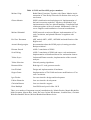
UNIVERSITY OF TÜBINGEN
WILHELM-SCHICKARD-INSTITUTE
FOR COMPUTER SCIENCE
Department of Computer Architecture
JavaNNS
Java Neural Network Simulator
User Manual, Version 1.1
Igor Fischer, Fabian Hennecke, Christian Bannes, Andreas Zell
Contents
1. Introduction .................................................................................................................. 4
1.1. How to read this manual....................................................................................... 4
2. Licensing and Acknowledgements .............................................................................. 5
2.1. License Agreement ............................................................................................... 5
2.2. Acknowledgments ................................................................................................ 6
3. Installation.................................................................................................................... 8
3.1. Running JavaNNS ................................................................................................ 8
4. A Quick Tour of JavaNNS........................................................................................... 9
4.1. Starting JavaNNS ................................................................................................. 9
4.2. Loading Files ........................................................................................................ 9
4.3. View Network....................................................................................................... 9
4.4. Training Network ................................................................................................. 9
4.5. Analyzing Network............................................................................................. 10
4.6. Creating a Network............................................................................................. 10
4.7. Graphical Network Display ................................................................................ 10
4.8. Training and Validation Pattern Sets.................................................................. 11
5. Network Creation and Editing ................................................................................... 12
5.1. Network View and Display Settings .................................................................. 12
5.2. Tools for Creating Networks .............................................................................. 13
5.3. Editing Units....................................................................................................... 14
6. Pattern Management................................................................................................... 15
7. Training and Pruning Networks ................................................................................. 16
8. Analyzing Networks................................................................................................... 18
8.1. Projection Panel.................................................................................................. 18
8.2. Weights Panel ..................................................................................................... 18
8.3. Analyzer.............................................................................................................. 19
9. Loading, Saving and Printing..................................................................................... 20
Appendix A: Kernel File Interface ................................................................................. 21
A.1. The ASCII Network File Format........................................................................ 21
A.2. Form of the Network File Eries.......................................................................... 21
A.3. Grammar of the Network Files........................................................................... 22
A.4. Grammar of the Pattern Files.............................................................................. 27
Appendix B: Example Network File .............................................................................. 30
B.1. Example 1:.......................................................................................................... 30
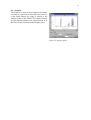
B.2. Example 2:.......................................................................................................... 32
4
1. Introduction
Java Neural Network Simulator (JavaNNS) is a simulator for neural networks developed at the
Wilhelm-Schickard-Institute for Computer Science (WSI) in Tübingen, Germany. It is based
on the Stuttgart Neural Network Simulator (SNNS) 4.2 kernel, with a new graphical user
interface written in Java set on top of it. As a consequence, the capabilities of JavaNNS are
mostly equal to the capabilities of the SNNS, whereas the user interface has been newly
designed and -- so we hope -- become easier and more intuitive to use. Some complex, but not
very often used features of the SNNS (e.g. three-dimensional display of neural networks) have
been left out or postponed for a later version, whereas some new, like the log panel, have been
introduced.
Besides the new user interface, a big advantage of JavaNNS is its increased platform independence. Whereas SNNS was developed with primarily Unix workstations in mind, JavaNNS
also runs on PCs, provided that the Java Runtime Environment is installed. As of writing of
this manual JavaNNS has been tested on:
• Windows NT
• Windows 2000
• RedHat Linux 6.1
• Solaris 7
• Mac OS X
with more to follow soon.
1.1. How to read this manual
Because of large similarities between SNNS and JavaNNS, this manual covers only the differences between the two. It should be read as a companion to the SNNS User Manual, available
from the WSI web site:
http://www-ra.informatik.uni-tuebingen.de/SNNS/
We suggest that you first read the SNNS Manual, in order to become acquainted with the theory of neural networks, the way they are implemented in the SNNS kernel and to get a basic
idea of the SNNS graphical user interface. If you are already familiar with SNNS, you can
skip this step and start directly with this manual.
In the next chapter, you will find the license agreement. Please read it carefully and make sure
that it is acceptable for you before installing and using JavaNNS. The installation process differs slightly for Windows and Unix machines and is described separately for each case. After
installing, we suggest that you follow our quick tour through the simulator to get the first
impression of how it is organized and used. The rest of the manual covers in more detail creating, manipulation and analyzing neural networks. You can skim it in the first reading and use
it later as a reference.
5
2. Licensing and Acknowledgements
JavaNNS is Copyright (c) 1996-2001 JavaNNS Group, Wilhelm-Schickard-Institute for Computer Science (WSI), University of Tübingen, Sand 1, 72076 Tübingen, Germany. It uses the
kernel of SNNS (Stuttgart Neural Network Simulator), which is Copyright (c) 1990-95 SNNS
Group, Institute for Parallel and Distributed High-Performance Systems (IPVR), University of
Stuttgart, Breitwiesenstrasse 20-22, 70565 Stuttgart, Germany.
Currently, JavaNNS is distributed by the University of Tübingen and only as a binary.
Although it is distributed free of charge, please note that it is NOT PUBLIC DOMAIN.
The JavaNNS License is gives you the freedom to give away verbatim copies of the JavaNNS
distribution (which include the license). We do not allow modified copies of our software or
software derived from it to be distributed. You may, however, distribute your modifications as
separate files along with our unmodified JavaNNS software. We encourage users to send
changes and improvements which would benefit many other users to us so that all users may
receive these improvements in a later version. The restriction not to distribute modified copies
is also useful to prevent bug reports from someone else's modifications.
For our protection, we want to make certain that everyone understands that there is NO WARRANTY OF ANY KIND for the JavaNNS software.
2.1. License Agreement
1. This License Agreement applies to the JavaNNS program and all accompanying programs
and files that are distributed with a notice placed by the copyright holder saying it may be
distributed under the terms of the JavaNNS License. 'JavaNNS', below, refers to any such
program or work, and a 'work based on JavaNNS' means either JavaNNS or any work containing JavaNNS or a portion of it, either verbatim or with modifications. Each licensee is
addressed as 'you'.
2. You may copy and distribute verbatim copies of the JavaNNS distribution as you receive
it, in any medium, provided that you conspicuously and appropriately publish on each
copy an appropriate copyright notice and disclaimer of warranty, keep intact all the notices
that refer to this License and to the absence of any warranty, and give any other recipients
of JavaNNS a copy of this license along with JavaNNS.
3. You may modify your copy or copies of JavaNNS or any portion of it only for your own
use. You may not distribute modified copies of JavaNNS. You may, however, distribute
your modifications as separate files (e.,g. new network or pattern files) along with our
unmodified JavaNNS software. We also encourage users to send changes and improvements which would benefit many other users to us so that all users may receive these
improvements in a later version. The restriction not to distribute modified copies is also
useful to prevent bug reports from someone else's modifications.
4. If you distribute copies of JavaNNS you may not charge anything except the cost for the
media and a fair estimate of the costs of computer time or network time directly attributable to the copying.
5. You may not copy, modify, sublicense, distribute or transfer JavaNNS except as expressly
provided under this License. Any attempt otherwise to copy, modify, sublicense, distribute
or transfer JavaNNS is void, and will automatically terminate your rights to use JavaNNS
under this License. However, parties who have received copies, or rights to use copies,
from you under this License will not have their licenses terminated so long as such parties
remain in full compliance.
6
6. By copying, distributing or modifying JavaNNS (or any work based on javaNNS) you
indicate your acceptance of this license to do so, and all its terms and conditions.
7. Each time you redistribute JavaNNS (or any work based on JavaNNS), the recipient automatically receives a license from the original licensor to copy, distribute or modify
JavaNNS subject to these terms and conditions. You may not impose any further restrictions on the recipients’ exercise of the rights granted herein.
8. Because JavaNNS is licensed free of charge, there is no warranty for it, to the extent permitted by applicable law. The copyright holders and/or other parties provide JavaNNS ’as
is’ without warranty of any kind, either expressed or implied, including, but not limited to,
the implied warranties of merchantability and fitness for a particular purpose. The entire
risk as to the quality and performance of JavaNNS is with you. Should the program prove
defective, you assume the cost of all necessary servicing, repair or correction.
9. In no event will any copyright holder, or any other party who may redistribute JavaNNS as
permitted above, be liable to you for damages, including any general, special, incidental or
consequential damages arising out of the use or inability to use JavaNNS (including but
not limited to loss of data or data being rendered inaccurate or losses sustained by you or
third parties or a failure of JavaNNS to operate with any other programs), even if such
holder or other party has been advised of the possibility of such damages.
2.2. Acknowledgments
JavaNNS is a joint effort of a large number of people, computer science students, research
assistants as well as faculty members at the Institute for Parallel and Distributed High Performance Systems (IPVR) at University of Stuttgart, the Wilhelm Schickard Institute of Computer Science at the University of Tübingen, and the European Particle Research Lab CERN in
Geneva.
The project to develop an efficient and portable neural network simulator which later became
SNNS was lead since 1989 by Dr. Andreas Zell, who designed SNNS and acted as advisor for
more than two dozen independent research and Master's thesis projects that made up SNNS,
JavaNNS and some of its applications. Over time the source grew to a total size of now 5MB
in 160.000+ lines of code. Research began under the supervision of Prof. Dr. Andreas Reuter
and Prof. Dr. Paul Levi. We are grateful for their support and for providing us with the necessary computer and network equipment.
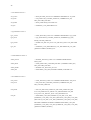
The following persons were directly involved in the SNNS project. They are listed in the order
in which they joined the SNNS team.
Table 1: SNNS and JavaNNS project members
Andreas Zell
Design of the SNNS simulator, SNNS project team leader.
Niels Mache
SNNS simulator kernel (really the heart of SNNS), parallel
SNNS kernel on MasPar MP-1216.
Tilman Sommer
original version of the graphical user interface XGUI with
integrated network editor, PostScript printing.
Ralf Hübner
SNNS simulator 3D graphical user interface, user interface
development (version 2.0 to 3.0).
Thomas Korb
SNNS network compiler and network description language
Nessus.
7
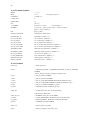
Table 1: SNNS and JavaNNS project members
Michael Vogt
Radial Basis Functions. Together with Günter Mamier implementation of Time Delay Networks. Definition of the new pattern format.
Günter Mamier
SNNS visualization and analyzing tools. Implementation of
the batch execution capability. Together with Michael Vogt
implementation of the new pattern handling. Compilation and
continuous update of the user manual. Maintenance of the ftp
server. Bugfixes and installation of external contributions.
Michael Schmalzl
SNNS network creation tool Bignet, implementation of Cascade Correlation, and printed character recognition with
SNNS.
Kai-Uwe Herrmann
ART models ART1, ART2, ARTMAP and modification of the
BigNet tool.
Artemis Hatzigeorgiou
documentation about the SNNS project, learning procedure
Backpercolation 1.
Dietmar Posselt
ANSI-C translation of SNNS.
Sven Döring
ANSI-C translation of SNNS and source code maintenance.
Implementation of distributed kernel for workstation clusters.
Tobias Soyez
Jordan and Elman networks, implementation of the network
analyzer.
Tobias Schreiner
Network pruning algorithms.
Bernward Kett
Redesign of C-code generator snns2c.
Jens Wieland
Design and implementation of batchman.
Jürgen Gatter
Implementation of TACOMA and some modifications of Cascade Correlation.
Igor Fischer
Java user interface design and development.
Fabian Hennecke
Java user interface development.
Christian Bannes
Java user interface support
Hans Rudolph
JavaNNS kernel port for Mac OS X
There are a number of important external contributions by: Martin Reczko, Martin Riedmiller,
Mark Seemann, Marcus Ritt, Jamie DeCoster Jochen Biedermann, Joachim Danz, Christian
Wehrfritz Randolf Werner, Michael Berthold and Bruno Orsier.
8
3. Installation
To be able to use JavaNNS, you have to have Java Runtime Environment (or JDK, which contains it) installed. JavaNNS has been tested to work with Java 1.3, Java 1.2.2 might also work,
though problems with file management have been reported in certain environments.
JavaNNS for Windows platforms is distributed as the zip file JavaNNS-Win.zip, and as
gzipped tar archive, like JavaNNS-LinuxIntel.tar.gz and JavaNNS-Solaris.tar.gz for other
operating systems. Unzip (unpack) the file into a folder of your choice. You should get:
1. JavaNNS.jar - the Java archive file containing the JavaNNS user interface classes
2. examples - folder with example networks, patterns etc.
3. manual - folder containing this manual
JavaNNS needs the kernel library in order to work properly. If you run JavaNNS the first time
on your machine a dialog will appear to ask you where to install the library.
JavaNNS then rememberes the location of the library by storing it in the file JavaNNS.properties, which is generated and placed into your home directory (Personal in Windows terminology). If you which to change properties, use Properties editor in the JavaNNS View menu.
You can delete the library or the JavaNNS.properties file any time you want. In that case the
library installation dialog will appear the next time you start JavaNNS.
3.1. Running JavaNNS
That’s all! Now you can start JavaNNS by typing:
java -jar JavaNNS.jar
from the command prompt or by clicking the JavaNNS.jar file from the graphical user interface.
9
4. A Quick Tour of JavaNNS
JavaNNS is a simulator for artificial neural networks, i.e. computational models inspired by
biological neural networks. It enables you to use predefined networks or create your own, to
train and to analyze them. If any of these terms is unknown to you, please refer to a book about
neural networks or to the SNNS User Manual - this manual describes only the usage of
JavaNNS.
4.1. Starting JavaNNS
To begin the tour, let’s start JavaNNS, as described in "Installing": type java -jar JavaNNS.jar
or, if using Windows, click the JavaNNS.bat file. After starting the program, its main window
opens. As we have started the program no parameters in the command line, the window is
empty, containing only the usual menu bar. Also, no network files have been loaded.
4.2. Loading Files
Use File/Open menu to open an example file: navigate to the examples directory and open the
files xor_untrained.net, and xor.pat - a simple network and a corresponding pattern file.
4.3. View Network
The main window still remains empty, so choose View/Network to display the network. You
should see a new window appearing, schematically showing a network, consisting of 4 units
(neurons) and links between them, in its main part. Neurons and links have different colors,
representing different values of unit activations and link weights. The colored bar on the left
edge of the window shows which color corresponds to which value and can be used as
reminder. The colors - and appearance in general - can be adjusted through View/Display Settings, which corresponds to the Display/Setup window in SNNS.
4.4. Training Network
Let us now train the network - reprogram its weights, so that it gives the desired output when
presented an input pattern. For that purpose, open the Control Panel in the Tools menu. The
Control Panel is, as in the SNNS, the most important window in the simulator, because almost
all modifications and manipulations of the network are done through it. We shall also open the
Error Graph window, in order to watch the training progress. Finally, to receive some textual
and numerical information, we can open the Log window. Both are accessible through the
View menu.
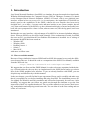
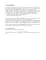
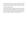
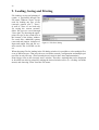
A sample screen shot with the windows open is shown in Figure 1.
The Control Panel is, contrary to the one in SNNS, divided into six tabs, each containing controls for specific purpose. For this introduction, let us switch directly to the learning tab. Here,
the user can choose the learning function, set its parameters, number of learning cycles and
update steps and finally perform network initialization and learning. The classic Backpropagation (equals Std_Backpropagation in SNNS) is the default learning function. As you can see,
for each learning function default parameters are provided.
Learning is performed by pressing one of the buttons: "Learn current" which performs training
with the currently selected pattern, and "Learn all", which trains the network with all patterns
from the pattern set. During learning, the error graph displays the error curve - the type of
error to be drawn is set on the left edge of the window. The error is also written into the log
window.
10
Figure 1: JavaNNS with XOR network, error graph, control and log panel
4.5. Analyzing Network
For analyzing the network and its performance, tools like Analyzer (in the Tools menu) and
Projection (in the View menu), already familiar to SNNS users, can be used. For Projection,
two input units and a hidden or output unit have to be selected in order for the menu item to
become enabled. The Projection Panel than displays the activation of the hidden or output unit
as a function of the two inputs. The activation is represented by color, so a colored rectangle is
obtained. Analyzer is used to show output or activation of a unit as a function of other unit’s
activation or of the input pattern. Its usage is similar to the Analyze panel in the SNNS.
4.6. Creating a Network
Now let’s create a network of our own. Choose File/New to remove the current network from
the simulator. Then, choose Create/Layers from the Tools menu. A window resembling the
Bignet tool of SNNS appears. Choose width and height "1", unit type "Input" and click "Create" to create a new layer. For the next layer, set height to five and the unit type to "Hidden"
and click "Create" again. Finally, create the output layer with the height of one and unit type
"Output" and close the window. To connect the created units, use Create/Connections from the
Tools menu. Simply choose "Connect feed-forward" and click "Connect". Doing that, you
have created a simple feed-forward neural network, with one input, five hidden and one output
unit. You can now close the Connections window, too.
4.7. Graphical Network Display
You can arrange units on the display manually, by clicking and dragging them with the mouse.
In fact, clicking a unit selects it, and dragging moves all selected units. To deselect a unit,
press the CTRL-Key on the keyboard and click it while still holding the key pressed. Using
11
View/View Settings, tab Units and Links, you can choose what to display above and under
each unit. Make sure that "Name" is selected as top label. Since the units have just been created, they are all called "noName". To change the names, choose "Names" from the Edit
menu. The top labels turn to text fields. Use the mouse to place the caret into each one and
enter some names. After you have finished, press "Enter" or click in an empty are of the display to turn the text fields to labels again.
4.8. Training and Validation Pattern Sets
To see how two pattern sets can be used for training and validation, load two pattern sets from
"examples" directory: trainMAP.pat and validMAP.pat. In the Control Panel, tab "Patterns",
select trainMap as the training set and validMAP as the validation set. Switch back to the
"Learning" tab and train the network. During training two curves are displayed in the Error
Graph: one, who’s color depends on the number of already displayed curves and which represents the error of the training set, and the other, pink one, which represents the error of the validation set. The validation set is normally used to avoid overtraining of a network. For more
information refer to the SNNS User Manual and other neural networks literature.
12
5. Network Creation and Editing
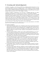
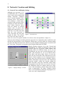
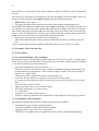
5.1. Network View and Display Settings
Although not necessary, it is
recommended that a network
view is open when creating and
editing networks. Network
view is opened through View/
Network menu. The network
view displays a visual representation of the network, which
comprises of units and connections (links) between them.
Units are drawn as colored
squares with 16 pixels side
length, and connections as colored lines. For both units and
links the color represents a
value: activation for units and
weight for links. The colored Figure 2: Network view
bar on the left edge of the network view serves as a quick reminder for color-to-value correspondence. (Figure 2)
Units are placed along an invisible grid in the network view. Optionally, above and below each
unit diverse unit properties can be displayed. Which ones, as well as grid size, chroma coding
for units and links and some more data are set in the Display Settings panel, accessible from
the View menu. This panel corresponds to the Display/Setup panel in SNNS.
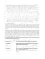
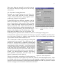
Figure 3: Display Settings - General
Display Settings comprise of two tabs: General and
Units&Links (or SOM for Kohonen tool). In tab
General, grid size (in pixels), subnet number and
chroma codes for different values can be set. In
Units&Links, the user can set which properties, like
name, unit activation etc. are to be shown above
(Top label) and below (Base label) of each unit.
Also, the user can decide if the connections are to be
shown, if their weights are to be displayed numerically and if the direction arrows should be drawn.
Sliders "Maximum expected value" and "Maximum
expected weight" control the chroma coding for
units and links, since they determine which value
corresponds to the full color, as set in the "General"
tab. Minimum values are simply taken to be negatives of the maximums, and for values between the
color is interpolated. The Slider "Weakest visible
link" is self-explanatory and helps keeping the network view more comprehensible.
13
Since more than one network view can be open at
the same time, Display Settings refer to the currently
selected one.
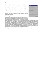
5.2. Tools for Creating Networks
Networks are created using two tools from the
"Tools" menu, both from the "Create" submenu:
"Layers" and "Connections". They together correspond to the "Bignet" tool in SNNS.
In JavaNNS layer has a different meaning as in the
SNNS. In JavaNNS, layer corresponds to a physical
layer of units that is being created. When creating
layers, width and height determine the number of
units in horizontal and vertical direction for the
layer. Top left position is updated automatically, but
can also be entered manually, and controls the layer’s Figure 4: Display Settings - Units and
Links
position in the display area. For all the data - width,
height and coordinates of the top left position - the
measuring unit is "grid size unit", which is set in the View/Display Settings panel.
In "Unit detail" segment of the window, the unit type (e.g. Input or Hidden), activation function of the units (Logistic by default), output function of the units (Identity by default), the
layer number and the subnet number are set.
The "Connections" window provides for creating links
(connections) between units. Three different ways are
possible for creating links: by manually selecting units
to connect ("Connect selected units"), by automatically
connecting the whole network in a feed-forward style
("Connect feed-forward") and by interconnecting those
in the same layer (Auto-associative). In case of feedforward networks, shortcut connections (links connecting units form non-adjacent layers) can optionally be
created. For auto-associative networks, self-connections (feedback connections from the output to the
input of a same unit) can be allowed.
Figure 5: Create Layers tool
Except for automatic generation of feed-forward connections, the user has to select units to be connected. Units are selected using the mouse, either
by clicking each unit, or by clicking the mouse and dragging a rectangle around units to be
selected. Units are deselected by clicking them while holding the CTRL key pressed. A simple
click in an empty area in a network view deselects all units.
14
Connecting selected units is a two-step process. In the first step,
the user selects units where the connections are to originate
(source units) and presses the button "Mark selected units as
source". In the second step, the user selects the receiving units
(targets) and presses the button, which is now labeled "Connect
source with selected units". For auto-associative connections it
suffices to select the desired units and press the "Connect
selected units" button.
Selected units can be dragged with the mouse in order to
change their positions.
5.3. Editing Units
Existing units can be edited by selecting them and then choosing Unit Properties from the Edit menu or Edit Units in the con- Figure 6: Create Links tool
text-sensitive menu, which is accessed by pressing the right
mouse button while over a unit. An extra window appears, displaying all editable unit properties, like name, type, activation etc. This method allows only for setting the same values for all
selected units. Alternatively, the user can edit values displayed as top and base labels of each
unit individually. For that purpose, the user has to choose from the Edit menu which property
he or she wants to edit. The labels displaying the property turn to entry fields, which can now
be edited. The fields are selected by the mouse and can be traversed by pressing the Tab key.
Pressing Enter accepts changes and turns the fields back to labels.
Changing activation values of units is useful if patterns are created manually.
15
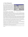
6. Pattern Management
Like in SNNS, patterns are organized in
pattern sets, which are stored as text files.
They can be loaded using the Open option
and saved using "Save data" (not Save!)
from the File menu. Further manipulation is
primarily performed from the Control Panel
(accessible from the Tools menu), in the
"Patterns" tab. Some simple manipulations
(adding, modifying, deleting) can be also
performed from the Patterns menu in the
main menu bar.
In the Control Panel, a pattern remapping Figure 7: Control Panel - Patterns
function and its parameters can be selected.
The two combo boxes - Training set and Validation set - are used for selecting the active training and validation set, respectively. Also, when new pattern sets are created (by pressing the
second button next to each of the combo boxes), the corresponding combo box becomes editable, so that the new pattern set can be given a name. The other button, adjacent to the combo
box, deletes the current pattern set from the memory.
Near the right edge of the panel, in the pre-last row, three more buttons serve for modifying
the current pattern set. Their function, from left to right, is: add, copy and delete pattern. Add
creates a new pattern from current input and output unit activations and adds it to the current
pattern set. Copy creates a new pattern, which is a verbatim copy of the currently selected one,
and adds it to the pattern set. Finally, the delete button deletes the currently selected pattern.
The current pattern is identified by its ordinal number in the pattern set. This number is displayed in a text field between arrow buttons in the bottom right corner of the panel. The arrow
buttons provide for navigating through the patterns in the currently selected set.
Some patterns can contain subpatterns of variable length. In that case, the tab "Subpatterns" is
enabled and provides for defining size and shape of subpatterns, as well as for navigating
through them. This corresponds to the Subpattern window in SNNS.
Propagating patterns through the network is done in the Update tab of the Control Panel. Same
navigational controls are provided as in the Patterns tab. Besides, the button between the
arrows propagates the current pattern through the network.
The same panel is also used for selecting the updating function and its parameters to be used in
training.
16
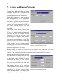
7. Training and Pruning Networks
Training is also performed through the
Control Panel. In the Initializing tab, an initialization function and its parameters can
be set. The Init button (also available in the
Learning tab) performs the initialization.
Under the Learning tab, the user can choose
the learning function, set its parameters,
number of learning cycles and update steps
and finally perform network initialization
and learning. The classic Backpropagation
(equals Std_Backpropagation in SNNS) is
the default learning function. For each
learning function default parameters are
provided.
The "Learn current" button performs training with the currently selected pattern and
"Learn all" with all patterns from the pattern set. In order to monitor learning
progress, it is useful to open the Error
Graph and/or Log window, both available
from the View menu. During learning, the
error graph displays the error curve. The
type of the error to be drawn is set through
the middle button located on the left edge
of the window. The arrow buttons near the
axes are used for scaling. The two buttons
in the left bottom corner clear the error
graph and toggle grid, respectively.
Figure 8: Control Panel - Init
Figure 9: Control Panel - Learning
During training, the error is also written into the log window. Also, many other useful information about the network are written there on diverse occasions. The log window corresponds
roughly to the command shell window from which SNNS is started in a Unix system.
Options and controls for pruning networks
are found under the Pruning tab in the Control Panel. Its contents corresponds mostly
to the Pruning window in SNNS. However,
contrary to the SNNS, the user does not
have to set the learning function to PruningFeedForward. In JavaNNS it is done automatically and transparently for him/her.
The learning function, as set under the
Learning tab, as well as number of cycles,
correspond to the data entered in "General
parameters for Training" section of the Figure 10: Control Panel - Pruning
SNNS’ Pruning window. In JavaNNS, pruning is performed by pressing the Prune button.
17
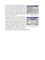
Cascade correlation and TACOMA learning are the
only exceptions to the concept of the Control Panel
being the central place for manipulating networks.
Because of the large number of parameters needed by
the two learning methods, a separate window, accessible from the Tools menu is used. Contrary to SNNS,
where parameters for cascade correlation and
TACOMA are dispersed between the Control Panel and
the Cascade window, in JavaNNS the Cascade window
alone covers all data and parameters needed for applying the two learning algorithms.
Figure 11: Cascade Correlation and
TACOMA - General
The window is divided into six tabs. Tabs "General",
"Modification" and "Learn" cover the parameters set in
SNNS in the section "General Parameters for Cascade"
of the Cascade window. Under the "Lear" tab of the
JavaNNS Cascade window, the learning function,
together with its parameters and the maximal number of
cascades (hidden units generated during learning) are
set. The "Init" tab is introduced for convenience and
provides for initializing network. Tabs "Candidates"
and "Output" correspond to "Parameters for Candidate Figure 12: Cascade Correlation and
TACOMA - Learning
Units" and "Parameters for Output Units" sections in
the SNNS window. The default learning method
invoked from the window is cascade correlation,
TACOMA can be set as a modification under the corresponding tab.
18
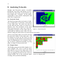
8. Analyzing Networks
Weights and Projection panels, accessible
through the View menu, and Analyzer, accessible from the Tools menu, can be used for getting insight into a network. All the panels
correspond to their SNNS counterparts and
differ only in appearance.
8.1. Projection Panel
The Projection panel shows activation of a hidden or output unit as a function of activations
of two input units. The panel can only be
opened when the three units are selected in a
network view. The activations of the input
units are drawn on the x- and y-axis, while corFigure 13: Projection panel
responding activations of the output unit are
represented by different pixel colors. For the
chroma coding, the same values as for the network view apply.
Arrows at the panel edges are used for moving
the projection window in the input space. The
two buttons on in the top left corner are used
for zooming, and the buttons in the bottom left
corner for adjusting the view resolution. Zooming can also be performed manually, by dragging a rectangle in the projection area.
8.2. Weights Panel
The Weights panel presents link weights as colored rectangles. The x-axis is used for source
units and the y-axis for the target units of the
links. The two buttons at the panel bottom are
used for toggling grid and for auto zoom for
optimal display. As in the projection panel,
zooming can be performed manually.
Figure 14: Weights panel
19
8.3. Analyzer
The Analyzer is used to show output or activation
of a unit as a function of other unit’s activation or
of the input pattern. Its usage is similar to the
Analyze panel in the SNNS. The control buttons
are also familiar and have the same function as in
the Error Graph, Projection and Weights panel.
Figure 15: Analyzer panel
20
9. Loading, Saving and Printing
File loading, saving and printing of
results is performed through the
File menu. Whereas "Open" can be
used for loading any type of file
(network, pattern, text...), "Save",
as well as "Save as" are used only
for saving the current network.
Other file types are saved through
"Save data", by choosing the appropriate file type in the combo box at
the bottom of the dialog window.
For result files, additional options
(start and end pattern, inclusion of
input and output files and file creation mode) like in SNNS can be
set.
Figure 16: File Save dialog
When choosing files for loading in the file dialog window it is possible to select multiple files,
even of different types. That way, the user can load a network, configuration and multiple pattern files in only one step. (This currently doesn’t work in the Linux implementation)
Print always refers to the currently active window. Therefore, anything that can be displayed
in JavaNNS can also be printed by making the desired window active (i.e. clicking it with the
mouse) and choosing "Print" from the File menu.
21
Appendix A: Kernel File Interface
A.1. The ASCII Network File Format
The ASCII representation of a network consists of the following parts:
• a header, which contains information about the net
• the definition of the teaching function
• the definition of the sites
•
the definition of cell types
• the definition of the default values for cells
• the enumeration of the cells with all their characteristics
• the list of connections
• a list of subnet numbers
• a list of layer numbers
All parts, except the header and the enumeration of the cells, may be omitted. Each part may
also be empty. It then consists only of the part title, the header line and the boarder marks (e.g.:
----|---|------).
Entries in the site definition section do not contain any empty columns. The only empty column in the type definition section may be the sites column, in which case the cells of this type
do not have sites.
Entries in the unit definition section have at least the columns no. (cell number) and position
filled. The entries (rows) are sorted by increasing cell number. If column typeName is filled,
the columns act func, out func, and sites remain empty.
Entries in the connection definition section have all columns filled. The respective cell does
not have a site, if the column site is empty. The entries are sorted by increasing number of the
target cell (column target). Each entry may have multiple entries in the column sources. In this
case, the entries (number of the source cell and the connection strength) are separated by a
comma and a blank, or by a comma and a newline (see example in the Appendix B).
The file may contain comment lines. Each line beginning with # is skipped by the SNNS-kernel.
A.2. Form of the Network File Eries
Columns are separated by the string " " (without ") . A row never exceeds 250 characters.
Strings may have arbitrary length. The compiler determines the length of each row containing
strings (maximum string length + 2). Within the columns, the strings are stored left adjusted.
Strings may not contain blanks, but all special characters except |. The first character of a
string has to be a letter.
Integers may have an arbitrary number of digits. Cell numbers arealways positive and not
zero. Position coordinates may be positive or negative. The compiler determines the length of
each row containing integers (maximum digit number + 2). Within the columns, the numbers
are stored right adjusted.
Floats are always stored in fixed length with the format Vx.yyyyy, where V is the sign (+, - or
blank), x is 0 or 1 and y is the rational part (5 digits behind the decimal point).
Rows containing floats are therefore always 10 characters long (8 + 1 blank on each side).
If a row contains several sites in the type or unit definition section, they are wri ten below each
other. They are separated in the following way: Directly after the first site fo lows a comma
22
and a newline \n. The next line starts with an arbitrary number of blanks or tabs in front of the
next site.
The source of a connection is described by a pair, the cell number and the strength of the connection. It always has the format nnn:Vx.yyyyy with the following meaning:
• nnn Number of the source
• Vx.yyyyy Strength of the connection as a float value (format as discribed above)
The compiler determines the width of the column nnn by the highest cell number present. The
cell numbers are written into the column right adjusted (according to the rules for integers).
The column Vx.yyyyy has fixed width. Several source pairs in an entry to the connection definition section/ are separated by a comma and a blank. If the list of source pairs exceeds the
length of one line, the line has to be parted after the following rule:
•
•
Separation is always between pairs, never within them.
The comma between pairs is always directly behind the last pair,i.e. remains in the old
line.
After a newline (\n) an arbitrary number of blanks or tabs may precede the next pair.
A.3. Grammar of the Network Files
A.3.1.Conventions
A.3.1.1. Lexical Elements of the Grammar
The lexical elements of the grammar which defines network files are listed as regular expresions. The first column lists the name of the symbol, the second the regular expresion defining
it. The third column may contain comments.
•
•
•
•
•
•
•
•
•
•
•
All terminals (characters) are put between ". . .".
Elements of sets are put between square brackets. Within the brackets, the characters represent themselves (even without ", and - defines a range of values. The class of digits is
defined, e.g. as ["0"-"9"].
Characters can be combined into groups with parenteses ().
x* means, that the character or group x can occur zero or more times.
x+ means, that the character or group x must occur at least once, but may occur several
times.
x? means, that x can be omitted.
x{n} means, that x has to occur exactly n times.
x|y means, that either x or y has to occur.
*, + and {} bind
strongest, ? is second, | binds weakest.
Groups or classes of characters are treated like a single character with respect to priority.
A.3.1.2.Definition of the Grammar
The Grammar defining the interface is listed in a special form of EBNF.
•
•
•
•
Parts between square brackets [] are facultative.
| separates alternatives (like with terminal symbols).
{x} means, that x may occur zero or more times.
CSTRING is everything that is recognized as string by the C programming language.
23
A.3.2.Terminal Symbols
WHITESPACE
{" "|"\n"|"\t"}
/* whitespaces */
BLANKS_TABS
{" "|"\t"}
W_COL_SEP
(" "|"\n"|"\t") {" "|"\n"|"\t"} "|" {" "|"\n"|"\t"}
/* only blanks or tabs */
/* at least one blank and the column separation */
COL_SEP
{" "|"\n"|"\t"} "|" {" "|"\n"|"\t"} /* column separation */
COMMA
{" "|"\n"|"\t"} "," {" "|"\n"|"\t"} /* at least the comma */
EOL
{" "|"\n"|"\t"} "\n" {" "|"\n"|"\t"} /* at least "\n" */
CUT
{" "|"\n"|"\t"} (" "|"\n"|"\t") {" "|"\n"|"\t"}
/* at least a blank, "\t", or "\n" */
COLON
":"
/* separation lines for different tables */
TWO_COLUMN_LINE
"-"+"|""-"+
THREE_COLUMN_LINE
"-"+"|""-"+"|""-"+
FOUR_COLUMN_LINE
"-"+"|""-"+"|""-"+"|""-"+
SIX_COLUMN_LINE
"-"+"|""-"+"|""-"+"|""-"+"|""-"+"|""-"+
SEVEN_COLUMN_LINE
"-"+"|""-"+"|""-"+"|""-"+"|""-"+"|""-"+"|""-"+
TEN_COLUMN_LINE
"-"+"|""-"+"|""-"+"|""-"+"|""-"+"|""-"+"|""-"+
"|""-"+"|""-"+"|""-"+
COMMENT
{{" "|"\n"|"\t"} "#" CSTRING "\n" {" "|"\n"|"\t"}}
VERSION
"V1.4-3D" | "V2.1" | "V3.0" /* version of SNNS */
SNNS
"SNNS network definition file" /* output file header */
/* eleven different headers */
GENERATED_AT
"generated at"
NETWORK_NAME
"network name :"
SOURCE_FILES
"source files"
NO.OF_UNITES
"no. of unites :"
NO.OF_CONNECTIONS
"no. of connections :"
NO.OF_UNIT_TYPES
"no. of unit types :"
NO.OF_SITE_TYPES
"no. of site types :"
LEARNING_FUNCTION
"learning function :"
PRUNING_FUNCTION
"pruning function :"
FF_LEARNING_FUNCTION
"subordinate learning function :"
UPDATE_FUNCTION
"update function :"
/* titles of the different sections */
24
UNIT_SECTION_TITLE
"unit definition section"
DEFAULT_SECTION_TITLE
"unit default section"
SITE_SECTION_TITLE
"site definition section"
TYPE_SECTION_TITLE
"type definition section"
CONNECTION_SECTION_TITLE
"connection definition section"
LAYER_SECTION_TITLE
"layer definition section"
SUBNET_SECTION_TITLE
"subnet definition section"
TRANSLATION_SECTION_TITLE
"3D translation section"
TIME_DELAY_SECTION_TITLE
"time delay section"
/* column-titles of the different tables */
NO
"no."
TYPE_NAME
"type name"
UNIT_NAME
"unit name"
ACT
"act"
BIAS
"bias"
ST
"st"
POSITION
"position"
SUBNET
"subnet"
LAYER
"layer"
ACT_FUNC
"act func"
OUT_FUNC
"out func"
SITES
"sites"
SITE_NAME
"site name"
SITE_FUNCTION
"site function"
NAME
"name"
TARGET
"target"
SITE
"site"
SOURCE:WEIGHT
"source:weight"
UNIT_NO
"unitNo."
DELTA_X
"delta x"
DELTA_Y
"delta y"
Z
"z"
LLN
"LLN"
LUN
"LUN"
TROFF
"Troff"
SOFF
"Soff"
CTYPE
"Ctype"
INTEGER
["0"-"9"]+
SFLOAT
["+" | " " | "-"] ["1" | "0"] "." ["0"-"9"]{5} /*signed float*/
/*integer */
STRING
("A"-"Z" | "a"-"z" | "|")+
/*string */
25
A.3.3.Grammar:
out_file
::= file_header sections
file_header
:= WHITESPACE COMMENT h_snns EOL COMMENT h_generated_at EOL
COMMENT h_network_name EOL COMMENT h_source_files EOL
COMMENT h_no.of_unites EOL COMMENT h_no.of_connections EOL
COMMENT h_no.of_unit_types EOL COMMENT h_no.of_site_types EOL
COMMENT h_learning_function EOL COMMENT h_update_function EOL
COMMENT h_pruning_function EOL
COMMENT ff_learning_function EOL
/* parts of the file-header */
h_snns
::= SNNS BLANKS_TABS VERSION
h_generated_at
::= GENERATED_AT BLANKS_TABS CSTRING
h_network_name
::= NETWORK_NAME BLANKS_TABS STRING
h_source_files
::= SOURCE_FILES [BLANKS_TABS COLON BLANKS_TABS CSTRING]
h_no.of_unites
::= NO.OF_UNITES BLANKS_TABS INTEGER
h_no.of_connections
::= NO.OF_CONNECTIONS BLANKS_TABS INTEGER
h_no.of_unit_types
::= NO.OF_UNIT_TYPES BLANKS_TABS INTEGER
h_no.of_site_types
::= NO.OF_SITE_TYPES BLANKS_TABS INTEGER
h_learning_function
::= LEARNING_FUNCTION BLANKS_TABS STRING
h_pruning_function
::= PRUNING_FUNCTION BLANKS_TABS STRING
h_ff_learning_function
::= FF_LEARNING_FUNCTION BLANKS_TABS STRING
h_update_function
::= UPDATE_FUNCTION BLANKS_TABS STRING
sections
::= COMMENT unit_section [COMMENT default_section]
[COMMENT site_section] [COMMENT type_section]
[COMMENT subnet_section] [COMMENT conn_section]
[COMMENT layer_section] [COMMENT trans_section]
[COMMENT time_delay_section] COMMENT
/* unit default section */
default_section
::= DEFAULT_SECTION_TITLE CUT COMMENT WHITESPACE
default_block
default_block
::= default_header SEVEN_COLUMN_LINE EOL
{COMMENT default_def} SEVEN_COLUMN_LINE EOL
default_header
::= ACT COL_SEP BIAS COL_SEP ST COL_SEP SUBNET COL_SEP
LAYER COL_SEP ACT_FUNC COL_SEP OUT_FUNC CUT
default_def
::= SFLOAT W_COL_SEP SFLOAT W_COL_SEP STRING W_COL_SEP
INTEGER W_COL_SEP INTEGER W_COL_SEP STRING W_COL_SEP
STRING CUT
26
/* site definition section */
site_section
::= SITE_SECTION_TITLE CUT COMMENT WHITESPACE site_block
site_block
::= site_header TWO_COLUMN_LINE EOL {COMMENT site_def}
TWO_COLUMN_LINE EOL
site_header
::= SITE_NAME SITE_FUNCTION CUT
site_def
::= STRING W_COL_SEP STRING CUT
/* type definition section */
type_section
::= TYPE_SECTION_TITLE CUT COMMENT WHITESPACE type_block
type_block
::= type_header FOUR_COLUMN_LINE EOL {COMMENT type_def}
FOUR_COLUMN_LINE EOL
type_header
::= NAME COL_SEP ACT_FUNC COL_SEP OUT_FUNC COL_SEP SITES
CUT
type_def
::= STRING W_COL_SEP STRING W_COL_SEP STRING W_COL_SEP
[{STRING COMMA} STRING] CUT
/* subnet definition section */
subnet_section
::= SUBNET_SECTION_TITLE CUT COMMENT WHITESPACE
subnet_block
subnet_block
::= subnet_header TWO_COLUMN_LINE EOL {COMMENT subnet_def}
subnet_header
::= SUBNET COL_SEP UNIT_NO CUT
subnet_def
::= INTEGER W_COL_SEP {INTEGER COMMA} INTEGER CUT
TWO_COLUMN_LINE EOL
/* unit definition section /*
unit_section
::= UNIT_SECTION_TITLE CUT COMMENT WHITESPACE unit_block
unit_block
::= unit_header TEN_COLUMN_LINE EOL {COMMENT unit_def}
TEN_COLUMN_LINE EOL
unit_header
::= NO COL_SEP TYPE_NAME COL_SEP UNIT_NAME COL_SEP
ACT COL_SEP BIAS COL_SEP ST COL_SEP POSITION COL_SEP
ACT_FUNC COL_SEP OUT_FUNC COL_SEP SITES CUT
unit_def
::= INTEGER W_COL_SEP ((STRING W_COL_SEP) | COL_SEP)
((STRING W_COL_SEP) | COL_SEP) ((SFLOAT W_COL_SEP) | COL_SEP)
((SFLOAT W_COL_SEP) | COL_SEP) ((STRING W_COL_SEP) | COL_SEP)
INTEGER COMMENT INTEGER COMMENT INTEGER W_COL_SEP
((STRING W_COL_SEP) | COL_SEP) ((STRING W_COL_SEP) | COL_SEP)
[{STRING COMMA} STRING]
27
/* connection definition section */
connection_section
::= CONNECTION_SECTION_TITLE CUT
COMMENT WHITESPACE connection_block
connection_block
::= connection_header THREE_COLUMN_LINE EOL
connection_header
::= TARGET COL_SEP SITE COL_SEP SOURCE:WEIGHT CUT
connection_def
::= ((INTEGER W_COL_SEP) | COL_SEP) STRING W_COL_SEP
{COMMENT connection_def} THREE_COLUMN_LINE EOL
{INTEGER WHITESPACE COLON WHITESPACE SFLOAT COMMA}
INTEGER WHITESPACE COLON WHITESPACE SFLOAT CUT
/* layer definition section */
layer_section
::= LAYER_SECTION_TITLE CUT COMMENT WHITESPACE layer_block
layer_block
::= layer_header TWO_COLUMN_LINE EOL {COMMENT layer_def}
TWO_COLUMN_LINE EOL
layer_header
::= LAYER COL_SEP UNIT_NO CUT
layer_def
::= INTEGER W_COL_SEP {INTEGER COMMENT} INTEGER CUT
/* 3D translation section */
translation_section
::= TRANSLATION_SECTION_TITLE CUT
COMMENT WHITESPACE translation_block
translation_block
::= translation_header THREE_COLUMN_LINE EOL
{COMMENT translation_def} THREE_COLUMN_LINE EOL
translation_header
::= DELTA_X COL_SEP DELTA_Y COL_SEP Z CUT
translation_def
::= INTEGER W_COL_SEP INTEGER W_COL_SEP INTEGER
/* time delay section */
td_section
::= TIME_DELAY_SECTION_TITLE CUT COMMENT WHITESPACE
td_block
td_block
::= td_header SIX_COLUMN_LINE EOL {COMMENT td_def}
SIX_COLUMN_LINE EOL
td_header
::= NO COL_SEP LLN COL_SEP LUN COL_SEP
TROFF COL_SEP SOFF COL_SEP CTYPE CUT
td_def
::= INTEGER W_COL_SEP INTEGER W_COL_SEP INTEGER W_COL_SEP
INTEGER W_COL_SEP INTEGER W_COL_SEP INTEGER W_COL_SEP
A.4. Grammar of the Pattern Files
The typographic conventions used for the pattern file grammar are the same as for the network
file grammar (see section A.3.1.1).
28
A.4.1.Terminal Symbols
WHITE
{" " | "\t"}
FREE
{^"\n"}
COMMENT
"#" FREE "\n"
/* anything up to EOL */
L_BRACKET
"["
R_BRACKET
"]"
INT
["0"-"9"]
V_NUMBER
[Vv]{INT}+"."{INT}+
NUMBER
[-+]?{{INT}+ | {INT}+{EXP} |{INT}+"."{INT}*({EXP})? |
/* version number */
{INT}*"."{INT}+({EXP})?}
EXP
[Ee][-+]?{INT}+
VERSION_HEADER
"SNNS pattern definition file"
GENERATED_AT
"generated at" {FREE}* "\n"
NO_OF_PATTERN
"No. of patterns" {WHITE}* ":"
NO_OF_INPUT
"No. of input units" {WHITE}* ":"
NO_OF_OUTPUT
"No. of output units" {WHITE}* ":"
NO_OF_VAR_IDIM
"No. of variable input dimensions" {WHITE}* ":"
NO_OF_VAR_ODIM
"No. of variable output dimensions" {WHITE}* ":"
MAXIMUM_IDIM
"Maximum input dimensions" {WHITE}* ":"
MAXIMUM_ODIM
"Maximum output dimensions" {WHITE}* ":"
NO_OF_CLASSES
"No. of classes" {WHITE}* ":"
CLASS_REDISTRIB
"Class redistribution" {WHITE}* ":"
REMAPFUNCTION
"Remap function" {WHITE}* ":"
REMAP_PARAM
"Remap parameters" {WHITE}* ":"
A.4.2.Grammar
pattern_file
::= header pattern_list
header
::= VERSION_HEADER V_NUMBER GENERATED_AT NO_OF_PATTERN
NUMBER
i_head [o_head] [vi_head] [vo_head] [cl_head] [rm_head]
i_head
::= NO_OF_INPUT NUMBER
o_head
::= NO_OF_OUTPUT NUMBER
vi_head
::= NO_OF_VAR_IDIM NUMBER MAXIMUM_IDIM actual_dim
vo_head
::= NO_OF_VAR_ODIM NUMBER MAXIMUM_ODIM actual_dim
cl_head
::= NO_OF_CLASSES NUMBER [cl_distrib]
rm_head
::= REMAPFUNCTION NAME [rm_params]
actual_dim
::= L_BRACKET actual_dim_rest R_BRACKET |
L_BRACKET R_BRACKET
actual_dim_rest
::= NUMBER | actual_dim_rest NUMBER
cl_distrib
::= CLASS_REDISTRIB L_BRACKET paramlist R_BRACKET
rm_params
::= REMAP_PARAM L_BRACKET paramlist R_BRACKET
paramlis
::= NUMBER | paramlist NUMBER
pattern_list
::= pattern | pattern_list pattern
pattern
::= pattern_start pattern_body pattern_class
29
pattern_start
::= [actual_dim]
pattern_body
::= NUMBER | pattern_body NUMBER
pattern_class
::= NUMBER | NAME
30
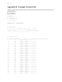
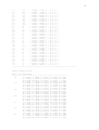
Appendix B: Example Network File
The lines in the connection definition section have been truncated to 80 characters per line for
printing purposes.
B.1. Example 1:
network name : klass
source files :
no. of units : 71
no. of connections : 610
no. of unit types : 0
no. of site types : 0
learning function : Std_Backpropagation
update function
: Topological_Order
unit default section :
act
| bias
| st | subnet | layer | act func
| out func
---------|----------|----|--------|-------|--------------|------------0.00000 | 0.00000 | h |
0 |
1 | Act_Logistic | Out_Identity
---------|----------|----|--------|-------|--------------|-------------
unit definition section :
no. | typeName | unitName | act
| bias
| st | position | act func | out func | sites
----|----------|----------|----------|----------|----|----------|----------|----------|------1 |
| u11
| 1.00000 | 0.00000 | i | 1, 1, 0 |||
2 |
| u12
| 0.00000 | 0.00000 | i | 2, 1, 0 |||
3 |
| u13
| 0.00000 | 0.00000 | i | 3, 1, 0 |||
4 |
| u14
| 0.00000 | 0.00000 | i | 4, 1, 0 |||
5 |
| u15
| 1.00000 | 0.00000 | i | 5, 1, 0 |||
6 |
| u21
| 1.00000 | 0.00000 | i | 1, 2, 0 |||
7 |
| u22
| 1.00000 | 0.00000 | i | 2, 2, 0 |||
8 |
| u23
| 0.00000 | 0.00000 | i | 3, 2, 0 |||
9 |
| u24
| 1.00000 | 0.00000 | i | 4, 2, 0 |||
10 |
| u25
| 1.00000 | 0.00000 | i | 5, 2, 0 |||
11 |
| u31
| 1.00000 | 0.00000 | i | 1, 3, 0 |||
12 |
| u32
| 0.00000 | 0.00000 | i | 2, 3, 0 |||
13 |
| u33
| 1.00000 | 0.00000 | i | 3, 3, 0 |||
14 |
| u34
| 0.00000 | 0.00000 | i | 4, 3, 0 |||
15 |
| u35
| 1.00000 | 0.00000 | i | 5, 3, 0 |||
16 |
| u41
| 1.00000 | 0.00000 | i | 1, 4, 0 |||
17 |
| u42
| 0.00000 | 0.00000 | i | 2, 4, 0 |||
18 |
| u43
| 0.00000 | 0.00000 | i | 3, 4, 0 |||
19 |
| u44
| 0.00000 | 0.00000 | i | 4, 4, 0 |||
20 |
| u45
| 1.00000 | 0.00000 | i | 5, 4, 0 |||
21 |
| u51
| 1.00000 | 0.00000 | i | 1, 5, 0 |||
22 |
| u52
| 0.00000 | 0.00000 | i | 2, 5, 0 |||
23 |
| u53
| 0.00000 | 0.00000 | i | 3, 5, 0 |||
24 |
| u54
| 0.00000 | 0.00000 | i | 4, 5, 0 |||
25 |
| u55
| 1.00000 | 0.00000 | i | 5, 5, 0 |||
26 |
| u61
| 1.00000 | 0.00000 | i | 1, 6, 0 |||
27 |
| u62
| 0.00000 | 0.00000 | i | 2, 6, 0 |||
28 |
| u63
| 0.00000 | 0.00000 | i | 3, 6, 0 |||
29 |
| u64
| 0.00000 | 0.00000 | i | 4, 6, 0 |||
30 |
| u65
| 1.00000 | 0.00000 | i | 5, 6, 0 |||
31 |
| u71
| 1.00000 | 0.00000 | i | 1, 7, 0 |||
32 |
| u72
| 0.00000 | 0.00000 | i | 2, 7, 0 |||
33 |
| u73
| 0.00000 | 0.00000 | i | 3, 7, 0 |||
34 |
| u74
| 0.00000 | 0.00000 | i | 4, 7, 0 |||
35 |
| u75
| 1.00000 | 0.00000 | i | 5, 7, 0 |||
31
36 |
| h1
| 0.99999 | 0.77763 | h | 8, 0, 0 |||
37 |
| h2
| 0.19389 | 2.17683 | h | 8, 1, 0 |||
38 |
| h3
| 1.00000 | 0.63820 | h | 8, 2, 0 |||
39 |
| h4
| 0.99997 | -1.39519 | h | 8, 3, 0 |||
40 |
| h5
| 0.00076 | 0.88637 | h | 8, 4, 0 |||
41 |
| h6
| 1.00000 | -0.23139 | h | 8, 5, 0 |||
42 |
| h7
| 0.94903 | 0.18078 | h | 8, 6, 0 |||
43 |
| h8
| 0.00000 | 1.37368 | h | 8, 7, 0 |||
44 |
| h9
| 0.99991 | 0.82651 | h | 8, 8, 0 |||
45 |
| h10
| 0.00000 | 1.76282 | h | 8, 9, 0 |||
46 |
| A
| 0.00972 | -1.66540 | o | 11, 1, 0 |||
47 |
| B
| 0.00072 | -0.29800 | o | 12, 1, 0 |||
48 |
| C
| 0.00007 | -2.24918 | o | 13, 1, 0 |||
49 |
| D
| 0.02159 | -5.85148 | o | 14, 1, 0 |||
50 |
| E
| 0.00225 | -2.33176 | o | 11, 2, 0 |||
51 |
| F
| 0.00052 | -1.34881 | o | 12, 2, 0 |||
52 |
| G
| 0.00082 | -1.92413 | o | 13, 2, 0 |||
53 |
| H
| 0.00766 | -1.82425 | o | 14, 2, 0 |||
54 |
| I
| 0.00038 | -1.83376 | o | 11, 3, 0 |||
55 |
| J
| 0.00001 | -0.87552 | o | 12, 3, 0 |||
56 |
| K
| 0.01608 | -2.20737 | o | 13, 3, 0 |||
57 |
| L
| 0.01430 | -1.28561 | o | 14, 3, 0 |||
58 |
| M
| 0.92158 | -1.86763 | o | 11, 4, 0 |||
59 |
| N
| 0.05265 | -3.52717 | o | 12, 4, 0 |||
60 |
| O
| 0.00024 | -1.82485 | o | 13, 4, 0 |||
61 |
| P
| 0.00031 | -0.20401 | o | 14, 4, 0 |||
62 |
| Q
| 0.00025 | -1.78383 | o | 11, 5, 0 |||
63 |
| R
| 0.00000 | -1.61928 | o | 12, 5, 0 |||
64 |
| S
| 0.00000 | -1.59970 | o | 13, 5, 0 |||
65 |
| T
| 0.00006 | -1.67939 | o | 14, 5, 0 |||
66 |
| U
| 0.01808 | -1.66126 | o | 11, 6, 0 |||
67 |
| V
| 0.00025 | -1.53883 | o | 12, 6, 0 |||
68 |
| W
| 0.01146 | -2.78012 | o | 13, 6, 0 |||
69 |
| X
| 0.00082 | -2.21905 | o | 14, 6, 0 |||
70 |
| Y
| 0.00007 | -2.31156 | o | 11, 7, 0 |||
71 |
| Z
| 0.00002 | -2.88812 | o | 12, 7, 0 |||
----|----------|----------|----------|----------|----|----------|----------|----------|-------
connection definition section :
target | site | source:weight
-------|------|---------------------------------------------------------------36 |
| 1: 0.95093, 6: 3.83328, 11: 1.54422, 16: 4.18840, 21: 4.59526
12: 2.30336, 17:-3.28721, 22:-0.43977, 27: 1.19506, 32:-0.84080
23:-4.97246, 28:-3.30117, 33: 3.26851, 4:-0.19479, 9: 1.33412
34:-1.02822, 5:-2.79300, 10:-1.97733, 15:-0.45209, 20:-0.61497
37 |
| 1:-0.93678, 6: 0.68963, 11:-0.94478, 16:-1.06968, 21:-0.47616
12: 2.62854, 17: 5.05391, 22:-0.37275, 27: 0.12598, 32: 0.27619
23:-1.45917, 28:-1.97934, 33: 1.01118, 4: 4.39595, 9:-2.78858
34:-0.14939, 5: 1.80792, 10: 3.66679, 15: 2.53150, 20:-1.07000
38 |
| 1: 2.44151, 6: 0.41693, 11: 2.12043, 16: 1.40761, 21: 1.83566
12:-0.55002, 17: 2.08524, 22: 0.63304, 27: 0.27301, 32:-2.49952
23: 3.14177, 28:-1.25889, 33:-6.35069, 4:-5.25082, 9: 0.01774
34:-3.66092, 5: 3.24401, 10: 1.88082, 15: 6.44985, 20: 3.24165
39 |
| 1: 5.17748, 6:-4.45709, 11:-0.65733, 16:-2.26190, 21:-2.69957
12:-1.43420, 17: 0.33409, 22:-0.74423, 27:-1.38010, 32: 3.08174
23:-4.42961, 28:-1.09858, 33: 2.09879, 4:-1.30835, 9: 0.79940
34: 1.99276, 5: 2.61433, 10:-3.56919, 15: 1.00952, 20: 2.86899
40 |
| 1: 3.03612, 6: 0.05247, 11:-3.20839, 16:-4.03382, 21:-3.55648
12: 0.23398, 17: 1.33895, 22: 6.03206, 27:-0.01723, 32: 0.09160
23:-1.07894, 28:-1.77930, 33: 1.59529, 4:-1.57236, 9: 0.74423
34:-0.13875, 5: 5.30719, 10: 2.13168, 15:-2.34832, 20:-5.00616
41 |
| 1:-4.41380, 6:-1.48152, 11:-2.62748, 16:-1.00557, 21:-0.06430
12: 3.93844, 17:-4.01591, 22: 0.76102, 27:-0.36823, 32: 0.54661
23: 4.15954, 28: 2.96118, 33:-3.30219, 4:-0.24202, 9: 1.56077
34:-0.20287, 5:-1.46062, 10: 1.79490, 15: 1.96920, 20: 3.72459
42 |
| 1: 1.97383, 6: 2.53253, 11: 2.04922, 16: 1.13969, 21: 1.81064
12: 0.32565, 17: 4.64358, 22: 1.02883, 27:-1.05720, 32:-0.71916
23:-1.00499, 28:-1.10925, 33:-3.18685, 4: 2.12575, 9: 0.36763
32
34:-0.18372, 5:-4.93490, 10: 0.26375, 15:-2.02860, 20:-5.43881
1: 0.07183, 6:-2.69081, 11:-1.24533, 16:-2.01347, 21:-1.36689
12:-2.11356, 17: 1.24788, 22: 1.23107, 27: 0.27674, 32:-2.45891
23: 5.17387, 28: 1.68170, 33:-2.30420, 4: 2.17011, 9: 0.86340
34:-2.23131, 5:-0.11916, 10:-4.39609, 15:-2.92706, 20:-5.43783
44 |
| 1:-1.27907, 6: 1.89325, 11:-0.60419, 16: 3.60368, 21: 4.24280
12:-2.77766, 17: 1.01698, 22:-1.97236, 27: 1.38773, 32:-2.55429
23: 1.95344, 28: 2.85157, 33:-0.55796, 4:-0.64082, 9: 1.92937
34:-2.71524, 5: 5.31087, 10:-2.08897, 15:-5.75332, 20: 2.43438
45 |
| 1:-1.22455, 6: 0.92594, 11: 1.13199, 16:-1.65062, 21:-1.41481
12:-3.04575, 17:-3.21280, 22:-0.23726, 27: 2.11836, 32: 2.23237
23: 5.96261, 28: 2.00822, 33: 2.97409, 4: 3.90943, 9: 1.54990
34: 2.42877, 5:-3.58017, 10: 2.31309, 15:-4.01833, 20: 0.28834
46 |
| 45:-3.97560, 44: 0.45729, 43:-1.16526, 42: 0.38939, 41: 2.80876
36:-4.04184
47 |
| 45:-4.88750, 44:-3.33955, 43:-1.72110, 42: 0.94756, 41:-2.24993
36: 0.14327
48 |
| 45: 1.02597, 44:-1.82773, 43:-1.04974, 42: 2.09881, 41:-0.53220
36: 2.75042
49 |
| 45: 1.58579, 44:-3.38572, 43:-0.89166, 42: 2.86233, 41: 2.25429
36: 1.92163
50 |
| 45:-2.95134, 44: 2.39376, 43:-2.95486, 42:-0.11771, 41:-2.41775
36:-0.73749
51 |
| 45:-4.16732, 44: 2.19092, 43: 3.46879, 42: 0.44175, 41:-2.47295
36:-0.40437
52 |
| 45: 1.78256, 44: 4.64443, 43:-2.50408, 42: 0.65889, 41:-2.52796
36:-1.73887
53 |
| 45:-3.64449, 44: 2.60025, 43:-1.57915, 42:-0.18638, 41:-4.14214
36:-4.29717
54 |
| 45:-0.45205, 44:-1.44890, 43: 5.23345, 42:-0.35289, 41: 2.43160
36:-1.99719
55 |
| 45: 0.46855, 44:-2.84431, 43:-1.80938, 42:-4.49606, 41: 1.16736
56 |
| 45:-1.27961, 44: 0.81393, 43: 2.66027, 42:-1.05007, 41: 0.47655
36: 0.72057
57 |
| 45:-1.21679, 44:-3.13145, 43:-0.69538, 42: 0.05268, 41:-3.12564
36: 2.16523
58 |
| 45:-3.44107, 44: 2.18362, 43:-1.60547, 42:-0.50213, 41: 2.47751
36: 1.05544
59 |
| 45:-5.06022, 44:-5.08796, 43:-0.74552, 42:-0.67009, 41: 2.90942
36: 1.10170
60 |
| 45:-0.03838, 44:-2.59148, 43:-0.98185, 42:-4.97460, 41: 1.03714
36: 4.49324
61 |
| 45:-3.65178, 44:-2.61389, 43:-1.76429, 42: 1.01853, 41:-3.90286
36: 0.46651
62 |
| 45: 1.17767, 44:-3.70962, 43:-1.11298, 42:-2.77810, 41: 2.22540
36:-0.65937
63 |
| 45: 1.52270, 44:-2.42352, 43: 2.59287, 42: 0.19606, 41:-3.00602
36:-3.14334
64 |
| 45: 3.00298, 44:-3.65709, 43:-1.65150, 42: 1.44547, 41:-3.98775
36:-4.02590
65 |
| 45: 0.56820, 44: 2.37122, 43: 2.89143, 42:-4.22975, 41:-2.32045
36:-2.17370
66 |
| 45:-4.13007, 44:-0.30654, 43:-0.63380, 42:-5.63405, 41:-1.78425
36: 1.46460
67 |
| 45: 1.66534, 44: 1.99220, 43:-1.22676, 42:-4.09076, 41:-3.58451
36: 1.40745
68 |
| 45: 0.60032, 44: 2.75100, 43:-1.17663, 42:-4.25699, 41: 1.60600
36:-4.23531
69 |
| 45:-4.31415, 44:-3.41717, 43:-0.77030, 42:-1.36290, 41: 1.92319
36: 0.28689
70 |
| 45: 0.54085, 44: 1.80036, 43:-2.19014, 42:-1.20720, 41: 1.54519
36:-2.79769
71 |
| 45: 0.00018, 44:-4.11360, 43: 0.85345, 42: 1.19947, 41: 1.22067
36:-3.29634
-------|------|---------------------------------------------------------------43 |
|
B.2. Example 2:
SNNS network definition file V3.0
33
generated at Fri Aug
3 00:25:42 1992
network name : xor
source files :
no. of units : 4
no. of connections : 5
no. of unit types : 2
no. of site types : 2
learning function : Quickprop
update function
: Topological_Order
site definition section :
site name | site function
-----------|-----------------inhibit
| Site_Pi
excite
| Site_WeightedSum
-----------|-----------------type definition section :
name
| act func
| out func
|sites
--------------|--------------|--------------|--------outType
| Act_Logistic | Out_Identity |
LongeroutType | Act_Logistic | Out_Identity |
--------------|--------------|--------------|--------unit default section :
act
| bias
| st | subnet | layer | act func
| out func
---------|----------|----|--------|-------|--------------|------------0.00000 | 0.00000 | h |
0 |
1 | Act_Logistic | Out_Identity
---------|----------|----|--------|-------|--------------|------------unit definition section :
no. | typeName
| unitName | act
| bias
| st | position | act func
----|---------------|----------|----------|----------|----|----------|--------1 |
| in_1
| 1.00000 | 0.00000 | i | 3,5,0
|||
2 |
| in_2
| 1.00000 | 0.00000 | i | 9,5,0
|||
3 |
| hidden
| 0.04728 | -3.08885 | h | 6,3,0
|||
4 |
| result
| 0.10377 | -2.54932 | o | 6,0,0
|||
----|---------------|----------|----------|----------|----|----------|---------
connection definition section :
target | site
| source:weight
-------|---------|------------------------------------------------------------3 |
| 1: 4.92521, 2:-4.83963
4 |
| 1:-4.67122, 2: 4.53903, 3:11.11523
-------|---------|-------------------------------------------------------------