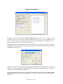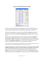
1
RspMatchEDT A Pre-Processor and Post-Processor for RspMatch2005 & RspMatch2009 User’s Manual Gustavo A. Ordóñez Copyright© 2005-2011 Gustavo A. Ordonez All rights reserved. No part of this work may be reproduced or transmitted in any form or by any means, electronic or mechanical, including photocopying, recording, or by any information storage or retrieval systems, without the prior written permission of GeoMotions, LLC. RspMatchEDT - Page No. ii RspMatchEDT A Pre-Processor & Post-Processor for RspMatch2005 & RspMatch2009 By Gustavo A. Ordóñez GeoMotions, LLC July 2011 - Revision RspMatchEDT - Page No. iii Terms and Conditions for Licensing the Software YOU SHOULD READ THE FOLLOWING TERMS AND CONDITIONS CAREFULLY BEFORE USING THE SOFTWARE. INSTALLATION OF THE SOFTWARE INTO YOUR COMPUTER INDICATES YOUR ACCEPTANCE OF THESE TERMS AND CONDITIONS. IF YOU DO NOT AGREE WITH THEM, YOU SHOULD RETURN THE PACKAGE PROMPTLY AND YOUR MONEY WILL BE REFUNDED. These programs are provided by the authors. Title to the media on which the software is recorded and to the documentation in support thereof is transferred to the customer, but title to the software is retained by the authors. GeoMotions, LLC owns all intellectual property in the programs. GeoMotions, LLC permits you to use the programs only in accordance with the terms of this agreement. You assume responsibility for the selection of the software to achieve your intended results and for the installation of the software, the use of and the results obtained from the software. License You may use the software on only one machine at any one time. You may copy the software for back up only in support of such use. You may not use, copy, modify, or transfer the software, or any copy, in whole or part, except as expressly provided in this document. You may not sell, sub-license, rent, or lease this software. You may not reverse engineer, decompile or disassemble the programs to obtain the source code. Although the software was tested, you are solely responsible for using and interpreting the results obtained from execution of the software. When first using the software, you should compare the results from the software with manual calculations and/or results from other computer software to verify the reliability of the program. The software is not a teaching tool for one-dimensional seismic site response analysis. The authors do not guarantee nor imply the accuracy or reliability of this software or related documentation. As such, they cannot be held responsible for incorrect results or damages resulting from the use of this software. It is the responsibility of the user to determine the usefulness and technical accuracy of this software in his/her own environment. This software was not developed as a network application. Thus, it should not be installed on a Network Server. Installation of the software onto your computer indicates your acceptance of the terms and conditions in this agreement. Terms The license is effective until terminated. You may terminate it any time by destroying the software together with any back-up copies. It will also terminate if you fail to comply with any term or condition of this agreement. You agree upon such termination to destroy the software together with any back-up copies, modifications, and/or merged portions in any form. Warranty The authors will correct any errors in the code at no charge after the purchase date of the software. Notification of a suspected error must be made in writing, with a complete listing of the input and output files and description of the error. If, in the judgment of the authors, the code does contain an error, the authors will (at their option) correct or replace the copy at no cost to the user or refund the initial purchase price of the software. These warranties are exclusive and in lieu of all other warranties, whether expressed or implied, including the implied warranties of merchantability, fitness for a particular purpose and non-infringement. No oral or written information or advice given by the authors, distributors, dealers or agents shall increase the scope of the above warranties or create any new warranties. Some states do not allow the exclusion of implied warranties, so the above exclusion may not apply to you. In that event, any implied warranties are limited in duration to ninety (90) days from the date of delivery of the software. This warranty gives you specific legal rights. You may have rights, which vary from state to state. Limitation of Liability The software is a complex program which requires engineering expertise to use correctly. The authors assume absolutely no responsibility for the correct use of this software. All results obtained should be carefully examined by an experienced professional engineer to determine if they are reasonable and accurate. Although the authors RspMatchEDT - Page No. iv have endeavored to make the software error free, the program is not and cannot be certified as infallible. Therefore, the authors make no warranty, either implicit or explicit, as to the correct performance or accuracy of this software. In no event shall the authors be liable to anyone for special, collateral, incidental, or consequential damage in connection with or arising out of purchase or use of this software. The sole and exclusive liability to the authors, regardless of the form of action, shall not exceed the purchase price of this software. USB Hardware Key Title to the USB Hardware Key(s) associated with a license belongs to GeoMotions, LLC. You are wholly responsible for maintaining and safeguarding the USB Hardware Key. We reserve the right to determine the cost of replacing a lost or stolen USB Hardware Key, up to and including the cost of a new license. Support The authors will provide telephone or electronic mail support, at no charge, to assist the licensee in the installation of the software on his or her computer system. Additionally, general assistance may be provided in aiding the licensee in understanding the capabilities of the various features of the software. However, no-cost assistance is not provided for help in applying the software to specific user-defined problems. We reserve the right to determine what qualifies as no-cost assistance, and what requires payment. In all instances, the user is encouraged to send the problem description and/or data files to the authors by electronic mail in order to minimize the amount of time spent trying to define the problem and/or to provide help with a problem. Copyright Notice The software and accompanying manual are copyrighted with all rights reserved by the authors, respectively. Under United States Copyright Laws, the software and its accompanying documentation may not be copied, in whole or in part, except to make a backup copy for archival purpose only. Any other copying, selling or otherwise distributing this software is hereby expressly forbidden. All products and brand names are trademarks and/or registered trademarks of their respective holders. Export Law Assurances You agree that the software will not be shipped, transferred or exported directly, into any country prohibited by the United States Export Administration Act and the regulations there under nor will be used for any purpose prohibited by the Act. If you do not agree to these terms and conditions, please return the full product with proof of purchase within 30 days for a full refund, minus shipping and handling costs. RspMatchEDT - Page No. v RspMatchEDT - Page No. vi RspMatchEDT User’s Manual RspMatchEDT - Page No. vii RspMatchEDT - Page No. viii Table of Contents RspMatchEDT ................................................................................................................................ 1 EDT File.................................................................................................................................. 1 Executing RspMatch2005 ....................................................................................................... 2 Processing RspMatch2005 Output Files ................................................................................. 2 RspMatch2005 ................................................................................................................................ 3 Specifying the Seed Accelerogram ......................................................................................... 3 Specifying the Target Spectrum.............................................................................................. 4 Running RspMatch2005 ......................................................................................................... 4 Output Files ............................................................................................................................. 5 Checking Output ..................................................................................................................... 5 Example Input Files ................................................................................................................ 6 RspMatchEDT Program Forms ...................................................................................................... 7 AASHTO's Response Spectra ................................................................................................. 9 Company & Project Information .......................................................................................... 11 Conversion of Ground Motion File....................................................................................... 13 Edit/Add Ground Motion File Information........................................................................... 22 EuroCode 8 Response Spectrum ........................................................................................... 26 Graphics Print Menu ............................................................................................................. 27 Graphics Window ................................................................................................................. 29 Ground Motion Attenuation Relations.................................................................................. 30 Ground Motion Parameters ................................................................................................... 37 IBC Response Spectra........................................................................................................... 39 Legend Text .......................................................................................................................... 41 NEHRP Response Spectra .................................................................................................... 42 Plot Object Motion................................................................................................................ 43 Print Menu ............................................................................................................................ 48 Report Form Development ................................................................................................... 50 Response Spectra for Ground Motion................................................................................... 52 Response Spectrum Plot Menu ............................................................................................. 55 Rjb & Rx Distance ................................................................................................................ 57 RspMatchEDT ...................................................................................................................... 59 SETARGET .......................................................................................................................... 67 Target/User Defined Response Spectrum ............................................................................. 70 View File ............................................................................................................................... 72 References ..................................................................................................................................... 75 RspMatchEDT - Page No. ix RspMatchEDT - Page No. x RspMatchEDT RspMatchEDT was developed as a Windows-based application that provides a user friendly graphical interface for RspMatch2005 & RspMatch2009. It presently includes the following: Forms used to enter the data to create an input file for RspMatch2005 & RspMatch2009. A feature to convert ground motion records to a format compatible with RspMatch or other computer programs. Numerous attenuation relations for estimating peak horizontal acceleration and velocity with distance; and, for the pseudo acceleration and pseudo velocity response spectra. Design spectra such as NEHRP, IBC, EuroCode and AASHTO. These spectra and those from attenuation relations can be plotted simultaneously with the spectra computed with RspMatch. An option to compute the response spectra for a ground motion. Printing of the output results for each graph in table form for inclusion in reports or other documents. The development process of RspMatchEDT is ongoing. The program will be continuously updated/upgraded based on input from users and modifications to the RspMatch2005 program. EDT File In this section, we will explain the main working file in RspMatchEDT. This file is identified by the extension *.EDT. This file stores the same information as an input file for RspMatch2005 plus other information such as the title and the name and path of the input file. To create an *.EDT file, you have two options. First, you may start from scratch by modifying the default data shown on the form upon starting of the program. Or, second, you can edit an existing file by opening a file using the Open command button. You will have to enter your project's specific data for each pass using the main editing form of RspMatchEDT. The latter allows you to simply modify existing data without the need to retype data that is similar to each project. Once you have edited the data for each pass, you can create an input file for RspMatch2005. An input file is created by clicking on the Save command button. This button will display the file dialog form that is used to save the EDT file; and, the file dialog form used to create the input file by saving the input data to a file. Further, when executing RspMatch2005 from within RspMatchEDT, it is necessary that RspMatch2005.EXE be located in the RspMatch2005 folder. For example, if RspMatchEDT was installed in the c:\RspMatchEDT folder, then the path to RspMatch2005.EXE will be: C:\RspMatchEDT\RspMatch2005\RspMatch2005.exe To differentiate the input file from the database file, you should give it a different name and extension. The file does not need to have the EDT extension; however, by default, when opening an existing file, RspMatchEDT will present you with a list of files that end with this extension. RspMatchEDT - Page No. 1 Executing RspMatch2005 After creating the input file, click on the RspMatch command button to execute RspMatch2005. The program will assume that the input file and all other data files needed are saved in the path shown on the Working Folder text box of the main menu form. Processing RspMatch2005 Output Files After a successful “run” of RspMatch2005, the program will generate a series of files. The names of these files are the same as that used for the input accelerogram file. However, the file extension will include a number that indicates the number of the adjustment pass from which the output file is created. The following files will be created: File Name Contents *.acX Adjusted acceleration (X is an integer from one to nine depending on the adjustment pass). Spectral accelerations of the adjusted accelerogram at the periods requested to be matched (X is an integer from one to nine depending on the adjustment pass). Summary of the misfit at each iteration. *.rsX *.itt Further information on these files is provided in the following section of this User‟s Manual. To compare the spectrum of the matched time history to the target spectrum, use the Convert command button to first convert the *.acX file to a format compatible with RspMatchEDT, and then the Spectra command button to compute the response spectrum and plot the spectra. Technical Support While advanced users and researchers prefer manipulation of the individual output files, the majority of the users prefer RspMatchEDT graphing options. The best way to learn these options (and the program) is to follow the step by step tutorial saved in the Manual folder. If you require additional help with running the program, you may e-mail to: [email protected] It is recommended to attach the *.EDT and input ground motion files to any e-mails when requesting technical support. This will help us to identify the cause of any problems and/or to better understand the questions. Free updates of the program can be downloaded from our web site at: http://www.geomotions.com The student version of the program is limited to 2 passes and 1 damping ratio. Also, graphs or tables can be printed, but not copied to the Clipboard. When printing results, a “Student Version” string of characters is also printed. The main purpose of the student version is to help the student learn about modification of ground motion files for use in seismic site response analysis. RspMatchEDT - Page No. 2 RspMatch2005 This section is a literal copy of the user‟s manual information provided with RspMatch2005 (Julian Bommer, 2007). This program performs a time domain modification of an acceleration time history to make it compatible with a user specified target spectrum. The methodology is based on that proposed by Lilhanand and Tseng (1987, 1988). The original computer code was written by N. A. Abrahamson (1993) and subsequently updated by J. Hancock et al. (Hancock et al. 2006). The modification of the time history can be performed with a variety of different modification models (wavelets). The wavelet adjustment preserves the long period non-stationary phasing of the original time history. As with finite element analysis and probabilistic seismic hazard analysis some degree of user experience is unavoidable to use this program successfully. In particular, the adjusted time series should always be examined to ensure that excessive adjustment has not been made; details of some useful checks are given in the latter part of this document. To run the code the user will need the program executable and three input files: 1. The seed accelerogram (accelerogram to be adjusted) 2. The input parameter file 3. The target spectrum file The RspMatch2005 will produce three output files for each adjustment pass: 1. The modified acceleration time series 2. A file containing the spectral response at the periods requested to be matched 3. A file containing the average and maximum misfit at each iteration These files will be described in the following sections. Values which are in italics can be modified by the user in the corresponding input files or input statements. A schematic of the program is given in Figure 1. Example files are provided, which are described at the end of this document. Specifying the Seed Accelerogram The seed accelerogram file should be given in the following format: Title nPts, dt Acc (maximum 80 characters in length) Number of acceleration points. Time step. Single column list (vector) of acceleration time series (Units of g) Careful selection of the seed accelerograms is important to minimize the wavelet adjustment required. A useful strategy is to select records using the RMS difference in normalized record and target spectral acceleration (based on the equation used by Ambraseys et al 2004): SARMS 1 N SAo Ti SAs Ti PGAs PGAo 2 RspMatchEDT - Page No. 3 (1) where N is the number of periods at which the spectral shape is specified, SA0(Ti) is the spectral acceleration from the record at period Ti, SAs(Ti) is the target spectral acceleration at the same period; PGA0 and PGAs are the peak ground acceleration of the accelerogram and the zero-period anchor point of the target spectrum. As the RMS spectral acceleration only matches spectral shape the seed accelerograms should be linearly scaled so that the amplitude of the spectral accelerations has a good match with the target before wavelet adjustment is conducted. Recent research indicates that linear scale factors of 10 can be used without causing a bias in the response if records are selected to match the spectral shape (Watson-Lamprey and Abrahamson, 2006). To ensure that a realistic match to the target scenario duration and energy distribution, it is recommended that the seed accelerograms has a similar magnitude as the target scenario earthquake (see Bommer and Acevedo 2004). If a suite of accelerograms are required it is preferable to select accelerograms from different earthquakes and recording stations to avoid bias in source, path or site effects. Accelerogram files should have the extension *.acc. Specifying the Target Spectrum The target spectral acceleration file should be constructed to the following format: Title (maximum 80 characters in length). nPer1, nDamp Number of data points in the target file and the number of damping values. Damp1, Damp2… Damping values corresponding to the above (e.g., “0.05 0.10” for 5% and 10% damping). Freq, T1, T2, SA1, SA2... Column arrays of the frequency, time1, time2 and spectral acceleration values (units of g) to be matched at each damping level. Time1 (T1) and time2 (T2) specify the start and end time at which the adjustment at each frequency can be applied. It is recommended that initially T1 is set to 0.0 and T2 set to a large number so that it will exceed the duration of the accelerogram (eg 1000.0). T1 and T2 are used to constrain the adjustment to a particular time window in the accelerogram. It is recommended that the target spectra are specified using evenly spaced points on a log period scale. This is because the bandwidth of the response is a ratio of the forcing frequency to the natural frequency; hence fewer points are required at long periods (low frequencies) to obtain a smooth spectral match. Using 40 target points per log10 period unit is a reasonable starting point. Target spectra files usually have the extension *.tgt. Running RspMatch2005 The program RspMatch2005 uses a user specified input file to run. It is recommended to give these files usually the extension *.inp. All of the parameters as they appear will be explained in the following section. The program is set up to adjust accelerograms with multiple passes, starting at short periods (high frequencies) and progressively adjusting longer periods (low frequencies). To facilitate this, the RspMatchEDT - Page No. 4 input file is divided into separate sections for each pass. The first two lines specify the accelerogram and number of passes and the following nineteen lines are repeated for each pass. The description for each line is shown on the RspMatchEDT section of this manual. Output Files The filenames of the output files are constructed using the filename of the input accelerogram. Different file extensions are used for different file types. The final number in the file extension specifies the adjustment pass from which the output is produced. Output files with the adjusted acceleration have the extension *.acX, where X is an integer from one to nine depending on the adjustment pass from which the output was produced. These files have the format: Header nPts, dt output Echo of the target spectrum file name. Number of data points and time step Array of acceleration (in g) Output files with the extension *.rsX provide details of the spectral acceleration of the adjusted accelerogram at the periods requested to be matched. It is important to check the miss-match of the adjusted accelerogram at both periods other than those requested to be matched. Files with the extension *.itt contain a summary of the misfit at each iteration. The average misfit over the range of target periods is given, as is the period and amplitude of the maximum misfit is also provided. The misfit at spectral period T is defined as: Misfit T SAT SAt arg et T SAt arg et T 100 (3) where SA(T) is the spectral acceleration of the adjusted ground motion at this iteration at period T and SAtarget(T) is the target spectral acceleration. Checking Output As with any analysis program it is important to check the output of RspMatch2005. The spectral match is best checked by plotting the spectral acceleration and displacement of the adjusted accelerogram with the target spectra. Both matched and unmatched points should be plotted. Although this can be achieved using the results from the files of the matched and unmatched spectral points, it can be more straight forward to employ a generic program designed to calculate the response spectra at a range of points. The program SeismoSignal (available free from www.SeismoSoft.com) is ideal for this task. SeismoSignal is particularly effective when combined with MS Excel as the both target and measured response can be plotted together. It is useful to plot spectral accelerations with period on a log axis so the high frequency motions are clear. Although it is desirable to get a good spectral match it is equally important to check that excessive modification to the original ground motion has not taken place. This should be conducted by comparing plots of the original and adjusted acceleration, velocity and displacement time series. The energy content introduced into the record should also be checked by plotting the build up of the Arias intensity, known as the Husid plot, (Arias 1970, Husid 1969) for both the original and adjusted accelerogram. Arias intensity is defined as: RspMatchEDT - Page No. 5 AI To a t dt 2g 2 g 0 Where g is the acceleration of gravity, ag is ground acceleration time history squared and To is the total duration of the accelerogram. The arias intensity and the Husid plot (and many other useful parameters) can also be easily calculated by using SeismoSignal (www.SeismoSoft.com). The adjustment procedure can introduce a slight drift in the displacement time series, even when displacement compatible wavelets are used. This is purely due to the accumulation of rounding errors. Rounding errors are more likely to occur with shorter period (high frequency) wavelets and less well refined output acceleration time series. To reduce rounding errors, and hence the potential for drift, it is beneficial if the output acceleration time series is defined with sufficiently closely spaced data points that the one cycle of the shortest period wavelet is defined by at least eight data points. The easiest method to increase the refinement of the output accelerogram using the dtFlag to interpolate additional data points from the input acceleration time series. Alternatively a baseline correction can be applied to the adjusted time series. Example Input Files Example input files are provided with the program as follows: 00794Tc.acc 10sRefineLog.tgt 00794Tc1.inp Sample seed accelerogram Sample target spectral acceleration file Sample RspMatch2005 input file The program can be run from the DOS prompt by typing RspMatch2005 <space> filename where filename is the name of the RspMatch2005 input file including the file extension. Alternatively, double clicking the executable in windows or entering only the program name in DOS will run the program; the program will then prompt the user for the filename of the RspMatch2005 input file. The program can also be run using a batch routine if multiple accelerograms need to be processed. RspMatchEDT - Page No. 6 RspMatchEDT Program Forms RspMatchEDT - Page No. 7 RspMatchEDT - Page No. 8 AASHTO's Response Spectra This form is used to define the coefficients to compute the AASHTO response spectra based on the following equations (AASHTO, 1994): Cs 1.2 A S T 2/3 C sm Where: Cs Csm A S T Tm 1.2 A S Tm2 / 3 = = = = = = elastic seismic response coefficient for single mode analysis elastic seismic response coefficient for multimodal analysis Acceleration coefficient from Article 3.2 Dimensionless coefficient for the soil profile characteristics of the site (Article 3.5). Period Period of the mth mode of vibration. RspMatchEDT uses the value of Acceleration Coefficient, A, to compute the spectra for a number of periods using the above equation. For single mode or multimodal analysis, the value of Cs will be > 2.5 A; and, for soil profiles type III or type IV in areas where A >= 0.3, Cs will not exceed 2.0 A. The spectra for multimodal analysis are obtained by selecting the Multimodal option. An x will appear in the check box when multimodal analysis is used by RspMatchEDT. Further, the Fundamental Mode option will be enabled when the Multimodal option is selected. If the Fundamental Mode option is not selected, then for soil profiles types III and IV and for periods less than 0.3 seconds, RspMatchEDT will use the following formula to determine Csm: C sm A 0.8 4Tm Further, for multimodal analysis, when Tm exceeds 4.0 seconds the value of Csm for that mode will be determined with the following formula: C sm 3 AS Tm4 / 3 RspMatchEDT - Page No. 9 The user needs to enter the value for A, and select the site classes. To select a site class, click on the check box next to the class. An x will appear in the box when the class is selected. You can select all of the classes. Once you enter a value for A and select at least one class, the Ok command button is enabled. You can click on Ok to return to the previous form. RspMatchEDT - Page No. 10 Company & Project Information This form is used to enter textual information about your company and/or project that will be printed together with your graph and form. The information that can be entered on this form is divided into two groups: 1) information that is constant such as your company name, address, etc.; and, 2) information that changes from project to project such as project number, dates, etc. When you create your own forms, you can enter a description for the form on the text box next to the Description label. This description can be up to 80 characters long, and will not be shown on the form. To enter information on the form, first type in the information in the Label column. This label is expected to be constant, e.g. “Project No.:”. Then enter the information that changes in the text box for the Information column, e.g. “99-1035”. Then enter the X and Y coordinates where the text will be printed on the paper. The origin of coordinates, i.e. X = 0 & Y = 0, is the upper left corner of the paper sheet. The string of text formed by the information on the Label and Information columns will be printed starting at the point defined by X and Y. If you want to print the string centered at this point, then click on the check box of the Center column to select it (an x is shown on the check box when this option is selected). The string will be vertically centered with respect to the Y coordinate. To change the font type, size, or style of a string, click on the Font command button to display the font dialog form. Select a different font, size, or style and then click on Ok to return to the form. The information for the string's font will be displayed on the Font, Style, and Size text boxes. Every time you move the cursor to a text box on the Label or Information columns, the characteristics of the font for the string will be displayed on the respective text boxes. You can also display a logo on the page at a specific location. The position of the logo is determined by the coordinates for the upper-left and bottom-right corners of a rectangle as entered in the coordinate text boxes at the bottom of the form. This logo should be a bitmap, metafile or an icon type file. To select a RspMatchEDT - Page No. 11 logo, click on the Logo command button to display the file dialog window, select a file, and then click on the Open command button. Then, enter the coordinates for the box where in the logo will be displayed. The example described in the following paragraph is for a letter size paper (8.5” x 11”) and portrait orientation. To change paper type or orientation, click on the Printer command button to display the printer dialog window. For this example, first place the cursor on the text box next to the Description label. Type in a description for the information, e.g. “RspMatchEDT standard form”. Press the Tab key to move the cursor to the text box on the Label column for string No. 1, and enter Project. Next, press the Tab key twice to move the cursor to the text box on the X left column and enter 6.05. Press the Tab key once, and enter 9.575 on the Y left column. Note that the string is now shown on the bottom right corner of the form. Next, follow the same procedure to enter the following: Label File No.: Date: Initials: X left 6.05 6.05 6.05 Y left 9.775 9.975 10.17 The coordinates in this example are such that the text will print on the bottom right corner of the form created in the example of the Report Form Development section of this manual. After you have entered the information, click on the Save command button to save the data on an ASCII text file. The data can be retrieved for future use using the Open command button. Each time you place the cursor on either the Label or Information columns the Add and Delete command buttons are enabled. If you want to add data for a new line, place the cursor on the line where the new line will be located, and click on the Add button. A new line will be created, and the coordinates and thickness for the new line will be the same as those for the line immediately below. Now, you need to modify the information for the coordinates and thickness for the new line. The Delete button is used to delete a line from the form. Place the cursor on either the Label or Information columns, and then click on the Delete button. The data for the line will be removed from the form, and the information for the other lines updated accordingly. The Reset command button will delete the information for all of the lines. RspMatchEDT - Page No. 12 Conversion of Ground Motion File This form is used to convert ground motion files to a format compatible with RspMatch2005; or to a format and units compatible with other software applications. The ground motion file used as input in RspMatch2005 is usually formed by a series of acceleration values in g‟s saved in a formatted way that is compatible with the Format statement used in the FORTRAN programming language. Today, the user can obtain ground motion records from a wide number of sources. However, these files are not uniform in their formatting or processing. For example, ground motion files can be downloaded through the Internet that are saved in units other than g‟s such as cm/sec2. Other records may include values for acceleration, velocity and displacement in the same file, each as a column of data. Thus, the main purpose of this form is to extract the acceleration data from the file, convert them to g‟s and save them to a formatted text file that can be used by RspMatch2005. This form has two other functions. First, it can be used to enter information about a new ground motion file and then add the information to the database of ground motion files used by RspMatchEDT. Second, the user can access the form used to edit information about a ground motion file in the database. Conversion of a ground motion file involves the following steps: 1) opening the original or source ground motion file; 2) defining the way the data in the source file are to be read; and, 3) defining the way the data will be written to the new converted ground motion file. For the first step, use the Open command button to display the Open Source Ground Motion File dialog form, change to a different folder and/or subdirectory if necessary, and click on the file that needs to be converted to select it. This file needs to be a text or ASCII file. Then click on the Open command button of the dialog form to open it. After a few seconds, the first few lines of the file (up to 99 lines) will be displayed on the top list box of the form. RspMatchEDT - Page No. 13 The first three characters displayed in red are the numbers of each row of data in the file followed by a “|”. These characters are not part of the source file and are only shown to number the rows. After the row numbers, the alphanumeric characters that constitute the information saved in the file for each row are shown. Note that the characters are displayed as blue on a white background, and that every tenth character is displayed in red. However, if the tenth character is a “blank space” then the character is not shown. This is done to guide the user when defining the order of the data in the file. During the second step, you need to define the way the data in the source file are to be read. To this end, there are six options available in RspMatchEDT: Other, PEER, USGS, RspMatch, PEER AT2 and PEER ACC. The first option, Other, is used to manually define the way the data are to be read. The PEER and USGS options are used to automatically convert files downloaded from the respective web sites; and, the RspMatch option is used to convert files created by the RspMatch2005 computer program. To select one of these options, click on the down-arrow of the Source File Type list to display the list of options, and select the option that applies to your file. The PEER option is used to convert files downloaded from the PEER Strong Motion Database at: http://peer.berkeley.edu/smcat/search.html The PEER AT2 option is used to convert files downloaded from the PEER Strong Motion Databases at: http://peer.berkeley.edu/nga/search.html http://peer2.berkeley.edu/peer_ground_motion_database/site The PEER ACC option is used to convert files downloaded from the PEER Ground Motion Database at: http://peer2.berkeley.edu/peer_ground_motion_database/site The USGS option is used to convert files created with the Interactive Deaggregation feature of the United States Geological Survey (USGS) web site at: http://eqint.cr.usgs.gov/eq-men/html/deaggint2002-06.html The files downloaded from either web site, PEER or USGS, should be saved as Text files. This is done by first, selecting the Save As… option of the File menu in your web browser. And second, by selecting the Text File (*.txt) option of the Save as type option list. When using the PEER or USGS option, some basic information needed to read the source file is displayed on some of the text boxes. For PEER files, it is assumed that the first 4 lines in the file are the header, and that the acceleration values in the file are in g‟s. Further, the program will assume that the fourth line of the header section includes the number of acceleration values and the time interval between acceleration values. Hence, the program will use the value next to the NPTS= string for the number of acceleration values, and the value next to the DT= string for the time interval. For example, in the section of the ground motion file shown below, it is assumed that there are 11800 acceleration values and that the time interval is 0.005 seconds. PEER STRONG MOTION DATABASE RECORD. PROCESSING BY PACIFIC ENGINEERING. CHI-CHI 09/20/99, ALS, E (CWB) ACCELERATION TIME HISTORY IN UNITS OF G. FILTER POINTS: HP=0.1 Hz LP=30.0 Hz NPTS= 11800, DT= .00500 SEC .9029319E-05 .9034156E-05 .9026870E-05 .9016792E-05 .9034652E-05 RspMatchEDT - Page No. 14 If the formatting or the information in the file do not match these assumptions, then it is recommended to use the Other option as explained below. The USGS option is similar to the PEER option in that specific information is searched to determine the number of acceleration values and the time interval. However, the USGS files do not have a fixed number of header lines. Accordingly, USGS files are first read to determine the number of header lines, and at the same time, determine the number of acceleration values and time interval. To this end, the program will first search for the “npw2, dt, total duration =” string. For example: npw2, dt, total duration = 16384 0.00500 81.9 When this string is found, it is assumed that the time interval is the second value, e.g. 0.005 sec for the string above. The program will then search for the “Begin Scaled Accelerogram Data” string and assume that the acceleration values start one line after this position. The program will count the number of lines of data until it finds the “END OF AGRAM DATA” string. It is also assumed that the acceleration values are in cm/sec2 units. Once the number of header lines, acceleration values and time interval are determined, the program will proceed to convert the ground motion file. Please note that the USGS files contain data for 6 seismograms. For example: am0, am0b_m0fa= 1.642E+25 0.000E+00 npw2, dt, total duration = 16384 0.00500 *** Begin Scaled Accelerogram Data *** T A1(cm/s2) A2 A3 0.0000 8.2623E-04 2.9951E-04 3.0377E-04 81.9 A4 A5 2.8430E-04 -3.0169E-04 A6 4.7918E-04 In the above section of a USGS file, the first column corresponds to the time for the acceleration value, and the A1 through A6 columns each correspond to a different seismogram. By default, the program will read the acceleration values for the first column of acceleration data, i.e. the A1 column. If you wish to obtain the data for any of the other acceleration columns, change the value on the Acceleration Column text box as explained below. Another option that applies to the USGS files is Match Sa. The motions downloaded from the USGS web site are no longer scaled to the probabilistic motion. For example, for the 1996 synthetic seismogram option, if the probabilistic 2-second spectral acceleration for the 2% probability of exceedance in 50 years was 0.1 g, then each seismogram was scaled so that its 2-second spectral acceleration, with 5% damping, was 0.1 g. This is no longer the case for the 2002 synthetic seismogram option. The Match Sa option can be used to scale the synthetic motions to the probabilistic value. The USGS file includes the following information that is used by RspMatchEDT to scale the motions: Fractional oscillator damping = 0.050 period= 1.000 **Agrams not scaled to PSHA SA level. Avg SA (cm/s/s) = 102.44 **Avg factor needed to match target probabilistic SA 3.5127 **PSHA MODAL r(km), amag, PSHA sa or pga(cm/s2)= 0.138E+03 0.900E+01 0.360E+03 On the first line above, the damping value and period for the Sa are shown. If this line is not found on the file, then it is assumed that the seismogram is for PGA. The second line indicates that the motion was not scaled, and that an average value of Sa of 102.44 cm/sec2 was obtained for the 1-second period from the synthetic motions generated without scaling. The third line notes that the ground motion values will need to be scaled by an average value of 3.5127 to obtain a motion with the corresponding probabilistic value of Sa. On the fourth line, the last value corresponds to the probabilistic value of Sa or PGA (Sa in the above example) that was obtained for your site. Hence, if the synthetic motions were scaled by a factor of 3.5127, their probabilistic value of Sa at 1-second would be 360 cm/sec2. To match the spectra value, RspMatchEDT - Page No. 15 RspMatchEDT will use the probabilistic Sa or PGA value from the fourth line (i.e. 360 for the above example), compute the response spectrum for the synthetic motion, and then use the computed value of Sa for the period of interest (i.e. 1 second for the above example) to obtain a scaling factor by dividing the probabilistic Sa by the computed Sa. The acceleration values for the motion will be multiplied by this factor to obtain the modified ground motion. The Hard Rock option is only enabled when processing USGS ground motion files. When this option is selected, the USGS B/C boundary type motion will be transformed to a hard rock, i.e. rock type A, motion. The motions are converted using the deamplification function presented by Park (2003). The third option used to convert files is Other. With this option, you can choose one of two alternatives: 1) Free Format Data: The data are separated by blank spaces and can be read sequentially one after another or by using a specific sequence; or, 2) Formatted Data: The data can be obtained by reading a specific number of characters (with or without blank spaces) sequentially or by using a specific sequence. Please note that if the data are separated by characters other than blank spaces, such as “,” or “tabs”, then the data may not be read properly. Free Format Data: If the data are separated by at least one, or more blank spaces, then select the Free Format option. Next, enter the number of acceleration values that are to be read from the file in the text box below the No. Values label. Then, enter the time interval between acceleration values in the text box below the Time Step label. This value is used when plotting the converted motion and when adding the information about the source or converted files to the database. Usually the first few lines in the source file provide information about the motion such as earthquake magnitude, station, etc.; these lines are considered herein as the “header” lines. Also, this is the number of lines that need to be skipped before reaching the section of the file where the acceleration values are located. Enter the number of header lines in the text box below the No. Header Lines label. If you selected the Free Format option, skip the next two text boxes and place the cursor on the text box below the Number of Columns label. When reading the acceleration values in free format, the values should be ordered in one of two ways. Either each row of data is formed only by values of acceleration; or, on each row of data, there are also other values. For the second type, each row of data may have a column for period, acceleration, velocity, and displacement. For example, in the section of the ground motion file below, each row of data is formed only by acceleration values. There are 10 values of acceleration (in cm/sec2) in each row: SAMPLES/SEC=100 FILTER TYPE=BUTTERWORTH CORNER= 0.10 ORDER=3 DATA TYPE=AC NO OF POINTS= 6228, UNITS=CM/SEC**2 -0.16 -0.16 -0.16 -0.16 -0.17 -0.18 -0.20 -0.20 -0.20 -0.22 -0.25 -0.27 -0.28 -0.27 -0.27 -0.29 -0.32 -0.35 -0.38 -0.39 If your source file is of the above type, skip the Number of Columns and Acceleration Column boxes, and place the cursor on the text box below the Format label. On the other hand, each row of data on the file below has one value for time, acceleration, velocity and displacement: m0444r01 8.0 25.6 147.6 75.9 0.65 sec cm/sec**2 cm/sec cm 0.00 -0.1934E+00 0.0000E+00 0.0000E+00 0.01 -0.1938E+00 -0.1900E-02 0.0000E+00 If the source file is of this second type, enter the total number of columns of data on each row. For example, for the above example you would enter a 4. Next, place the cursor on the text box below the Acceleration Column. In this text box, you enter the number of the column that forms the acceleration value. In the above example this is the second column, thus you would enter a 2. Then place the cursor on the Format text box. RspMatchEDT - Page No. 16 Formatted Data: If you did not select the Free Format option, then you need to provide either the number of values per row and the length as number of characters of the values; or, the number of data columns per row, the number of the column with the acceleration values and the length as number of characters of the columns. For the first alternative, you need to define the way the values are separated in each row by indicating the number of values per row and the number of characters that form each value. The number of characters should be the same for every value. For example: 4 values per row, each value is 15 characters long including blank spaces and exponent: -.1059027E-04 -.1461820E-04 -.1690261E-04 -.1506594E-04 8 values per row, each value is 9 characters long including blank spaces: 0.00000 -0.00434 0.00860 0.00540 -0.00565 -0.00944 -0.00369 -0.00669 8 values per row, each value is 9 characters long: -0.000001-0.000002-0.000001-0.000001 0.000000 0.000001 0.000000-0.000001 After you have entered the data for number of values, time step, and number of header lines, place the cursor on the text box below the Values per Line label, and enter the number of values that are included in each line of data (for the above examples: 4, or 8, or 8, respectively). Next, place the cursor on the text box below the No. Digits label and enter the number of characters that form each value (for the above examples: 15, or 9, or 9, respectively). Then enter the rest of the information as described previously. For the second alternative, you need to provide the number of data columns on each row, the number of the acceleration column, and the number of characters that form each column. For example: m0444r01 8.0 25.6 147.6 75.9 0.65 sec cm/sec**2 cm/sec cm 0.00 -0.1934E+00 0.0000E+00 0.0000E+00 0.01 -0.1938E+00 -0.1900E-02 0.0000E+00 In the above section of a ground motion file, there are 4 columns of data per row (one each for time, acceleration, velocity and displacement), the second column is the acceleration value, and each value is 12 characters long including blank spaces and exponent. Thus, after entering data for number of values, time step, and number of header lines, place the cursor on the text box below the No. Digits label and enter the number of characters that form each value (e.g. 12). Then, place the cursor on the text box below the Number of Columns label and enter the total number of columns of data on each row. For the above example, you would enter a 4. Next, place the cursor on the text box below the Acceleration Column. In this text box, you enter the number of the column that forms the acceleration value. In the above example this is the second column, thus you would enter a 2. To continue with the conversion of the file, enter the rest of the information as described previously. In the third step, you will define how the data will be written to the converted file. First, define the format, i.e. the way the data are written to the file, of the acceleration values. This is based on the syntax used in the Format statement of the FORTRAN computer language. In this statement edit descriptors specify how the values are read. In this feature of RspMatchEDT the only two edit descriptors supported by RspMatchEDT are: Fw.d Real values RspMatchEDT - Page No. 17 Ew.d [Ee] Real values with exponents In these descriptors, the field is w characters wide, with a fractional part d decimal digits wide, and an optional exponent width of e. Remember that the field w also includes any blank spaces. You can also indicate that a given data format is repeated a number of times. For example, 8F9.6 repeats a ninecharacter real value with six decimal digits descriptor eight times. The first character on the format field should be a “(” and the last character a “)”, e.g. (8F9.6). Examples of data saved in the ground motion files included with RspMatchEDT and the format used to define them follow: Format: (4E15.8E2) or (4E15.8): -.10590270E-04 -.14618200E-04 -.16902610E-04 -.15065940E-04 Format: (8F9.5): 0.00000 -0.00434 0.00860 0.00540 -0.00565 -0.00944 -0.00369 -0.00669 Format: (8F10.6): -0.000001 -0.000001 -0.000001 -0.000001 0.000000 0.000000 0.000000 0.000001 If you use the “E” descriptor and do not provide a value for exponent width, “e”, RspMatchEDT will use a default value of 2. Depending on the number of decimal figures used for the acceleration values in the converted file, the velocity or displacement time histories obtained by double integration of the converted acceleration time history may not be correct, e.g. they may increase or decrease without bounds. Accordingly, it is recommended to use as many decimal figures as possible when converting the file. Next, you need to select a factor to convert the acceleration values in the source file to units compatible with RspMatch2005, i.e. fractions of acceleration of gravity (g‟s), if necessary; or, to other units if you wish to use the converted data as input for another software application. This can be done by selecting a factor that represents the units of the acceleration data in the source file from the list of options shown on the Source Units list box; and, by selecting the units of the converted file from the list of options shown on the Output Units list. After selecting the units, a multiplication factor will be displayed on the Multiplier box. This is the multiplication factor that will be used to convert the values from the units shown on the Source Units list box to the units shown on the Output Units list box. For example, to convert values of acceleration from cm/sec2 to g‟s, you need to divide each value by 980.665 cm/sec2; which is equivalent to multiplying each value by 1/980.665 = 0.00102. In the program, this is done by selecting the cm/sec^2 option of the Source Units list and the g’s option of the Output Units list, respectively. If the accelerations in the source file are in units that are not shown in the list, select the Other option of the Source Units list, and then enter a multiplication factor in the Multiplier text box. This multiplication factor should be appropriate to convert the source acceleration data to the units shown on the Output Units list. For example: WESTERN WASHINGTON EARTHQUAKE APR 13, 1949 - 1156 PST EPICENTER 47 06 00N,122 42 00W INSTR PERIOD 0.0770 SEC DAMPING 0.574 NO. OF POINTS 1094 DURATION 89.16 SEC UNITS ARE SEC AND G/10. RMS ACCLN OF COMPLETE RECORD 0.2455 G/10. ACCELEROGRAM IS BAND-PASS FILTERED BETWEEN 0.070 AND 25.000 4454 INSTRUMENT AND BASELINE CORRECTED DATA AT EQUALLY-SPACED INTERVALS OF 0.02 SEC. PEAK ACCELERATION 161.63023 CMS/SEC/SEC AT 10.9400 SEC RspMatchEDT - Page No. 18 55 31 42 42 23 43 CYC/SEC -152 -176 -234 29 -147 -176 -51 -49 27 -309 86 86 -364 88 26 -125 -69 42 134 -103 26 111 -75 -185 17 -65 -181 The fifth line of the header section indicates that the units are seconds and G/10, and from the tenth line you can see that the acceleration values are given in cm/sec2. Thus, to convert the values to g‟s, you need first to divide each value by 10, and then divide the result by 980.665. For example for the first value of 152: 152 10 0.015500 980.665 However, this is equivalent to multiplying each value by a factor of (1 / 9806.65) or 0.000102. Thus, you would enter a value of 0.000102 in the Multiplier text box. If you select the Other option of the Output Units list, you can enter a description of the other units (e.g. gals) in the Other Units text box. The RspMatch2005 and RspMatch2009 options of the Output Units list are used to convert files to a format compatible with the RspMatch2005 or RspMatch2009 computer programs, respectively. After selecting the multiplication factor, place the cursor on the text box below the Database Header Line label. Here you would enter a value that represents the line from the header section that will be used to identify the converted file in the database of ground motion files. For example, for the above record, you could use the first line to be included in the database, thus you would enter a 1. The last information needed before you convert the file is the number of the lines from the header section in the source file that you would like to include in the converted file. To do this, place the cursor on the first text box below the Lines from Source Header to be included in Converted Ground Motion File label. Here you can select a specific line, or select a range of lines. To select one line, just enter the number of the line in the text box. For example to select the first line from the above file enter a 1. To select a range of lines, enter the number of the first line in the range followed by a “-” and then the number of the last line in the range. For example, if you would like to select the first five lines of the above header you would enter 1-5 in the text box. There are 3 text boxes in this section that you can use to select different lines from the header section. By default, the first four lines in the header of the converted file will be created by RspMatchEDT. The lines will include the name and path of the source file, the units of the acceleration values, the number of acceleration values in the converted file (which may be slightly different from the original number in the source file), the time step of the acceleration time history, and the format string used to write the data to the file. These four lines will provide valuable information if the file is used with a different software application. U After you have entered the above information, you need to enter the name and path of the converted file. A default file name and path are shown on the box next to the Converted Ground Motion File label. If you would like to select a different file, first click on the Save command button to display the Save Converted Ground Motion File dialog form. Enter the name of the file on the text box next to the File name label, or use the mouse to select a file by highlighting it. Then click on the Save command button to return to the conversion form. Now, click on the Convert command button to convert the source file to the units and format you selected. After a few seconds, the first few lines (up to 99) of the converted file will be shown on the bottom list box. U U RspMatchEDT - Page No. 19 U After you have converted the file, you can plot the resulting motion using the Plot command button. You can also add information about this motion in the database of ground motions using the Dbase command button. Refer to the Edit/Add Ground Motion File Information section of this manual for further information. The Spectra command button is used to display the Response Spectra for Ground Motion form. This form can be used to compute the response spectra for the converted ground motion. The following web sites provide ground motion records for download. Please note that the following Internet addresses were valid at the time this User‟s Manual was updated. 1. PEER Strong Motion Databases: These databases contain over 1000 records from 140 earthquakes from tectonically active regions. http://peer.berkeley.edu/smcat/ http://peer.berkeley.edu/nga/search.html 2. Cosmos Virtual Data Center http://db.cosmos-eq.org/scripts/earthquakes.plx It is highly recommended that you use the above web sites to search for records given specific characteristics (e.g. mechanism, soil classification, magnitude, etc.). When downloading a file from an internet site, you need to save the file as a text file. Once you have an appropriate record for your analysis, you may need to transform the record to a format compatible with RspMatchEDT. You can use the Ground Motion File Utilities: Conversion & Database option of the Main Menu to convert the file. Adding Information about a Ground Motion File to the Database: To do this, first click on the Ground Motion File Utilities: Conversion & Database option of the Main Menu form to select it. Then, click on the Ok button to display the conversion form. Next, click on the Open command button to display the Open Source Ground Motion File dialog form. Change to the folder and subdirectory where the file is located if necessary, click on the file to highlight it, and then use the Open button to open the file and return to the conversion form. After a few seconds, the first few lines of the file (up to 99 lines) will be shown on the top list box of the form. Once the file is opened, you need to enter as a minimum the information requested in the No. Values, Time Step, No. Header Lines, Values per Line, Format and Database Header Line text boxes as described in the previous section. Note that in this case, the information that you enter in the Format text box refers to the file that you want to add to the database. If you do not enter a value for “Values per Line”, this information will be obtained from the data entered in the format text box. After entering this information, click on the Dbase command button to display the Edit/Add Ground Motion File Information form. Refer to that section on this manual for further information. Editing the Database of Ground Motion Files: This form also allows you to access the form used to edit the information available in the database of ground motion files. For more information about the database, refer to the Database of Earthquake Records section of this manual. To access the editor form, click on the Dbase command button to display the Edit/Add Ground Motion File Information RspMatchEDT - Page No. 20 form. Refer to that section of this manual for more information about editing the database. Please note that to access the database form, you should not open a file first. RspMatchEDT - Page No. 21 Edit/Add Ground Motion File Information This form is used to edit the database of ground motion files used by RspMatchEDT. The information about the files (e.g. file name, number of values, etc.) is saved in the RSPMATCHEDT.EQ file and can be accessed by different features of RspMatchEDT to get the information for the ground motion. For example, this database can be accessed from the response spectra form to select a ground motion for which the response spectra is computed. The editing functions that can be performed with this form are twofold. First, you can edit the data for an existing ground motion file, or you can remove a file from the database. Second, you can add the information about a new file in the database. Edit Information about a Ground Motion File: To display this form, you need to first select the Ground Motion File Utilities: Conversion & Database option of the Analyses & Utilities form and then click on the Ok command button. This will display the Conversion of Ground Motion File form. In this second form click on the Dbase command button to display the editing form. Once this form is displayed, you can edit the information by entering the new values in their respective text boxes. In the text box below the Description of Ground Motion File used in Database enter a string up to 128 characters long that describes the motion and that is displayed in the list box. For example, the first ground motion in the database shown above is identified as Alaska (7/3072) – Sitka Record, M: 7.5, Dis: 48 km, Amax: 0.091g, Rock outcrop. The name of the file and a path are entered in the text box below the Ground Motion File text box. The information in this text box can be added to the information shown on the Path to Earthquake Files text box to define the path to the file. For example, when executing RspMatchEDT the path to the first ground motion will be specified as c:\RspMatchEDT\quakes\alaska.eq when the path option is selected. You can also enter the name and a path if you saved the files in different subdirectories. For example, you can enter quakes\alaska.eq if the file is saved in the quakes subdirectory, and then on the path option you would select the c:\RspMatchEDT folder as the path where the file is located. Use the Directory command button to choose the path to the directory where the earthquake motion files are stored. After clicking on this button, the Path to Earthquake Files form will be displayed. Use the RspMatchEDT - Page No. 22 mouse to select the drive and directory, and then click on the Ok button. The directory will be displayed on the text box next to the Path to Earthquake Files label. The total number of acceleration values that form the object motion file is entered in the text box below the No. Values label. For the above example, there are 2048 values in the file. In the text box below the Time Step label, enter the time interval between each acceleration value. For this example, it is 0.02 seconds. The peak acceleration value of the ground motion can be entered in the text box below the Max. Acc. label. Entering this value is optional. In the text box below the No. Header label enter the number of lines at the beginning of the file that are used to describe the object motion. In the above example, the first three lines are the header lines. In the text box below the Values/Line label, enter the number of acceleration values on each line of the file. For the above example, there are 8 values on each line. The number entered in this box is used with the information entered in the Format text box to determine how many values are to be read from each row of data in the file. Other examples of the information entered in this box are: In the line below there are 4 values separated by blank spaces: -.1059027E-04 -.1461820E-04 -.1690261E-04 -.1506594E-04 In the line below there are 8 values. Note that there are no blank spaces separating the values when a negative sign is included: -0.000001-0.000001-0.000001-0.000001 0.000000 0.000000 0.000000 0.000001 In the line below, there are 8 values, and there are blank spaces separating the values. The last number (e.g. 1) only identifies the row number. Thus, you would enter an 8 in this cell for this specific example: 0.00000 -0.00434 0.00860 0.00540 -0.00565 -0.00944 -0.00369 -0.00669 1 The last information needed for the file is the Format value. The format string tells RspMatchEDT how to read the ground motion values from the file. This string is based on the syntax used in the Format statement of the FORTRAN computer language. In this statement edit descriptors specify how the values are read. The edit descriptors supported by RspMatchEDT in this feature are: Fw.d Ew.d [Ee] Gw.d Dw.d Iw Real values Real values with exponents Real values, extended range Double-precision real values Integer values In these descriptors, the field is w characters wide, with a fractional part d decimal digits wide, and an optional exponent width of e. Remember that the field w also includes any blank spaces and the sign. You can also indicate that a given data format is repeated a number of times. For example, 8F9.6 repeats a nine-character real value with six decimal digits descriptor eight times. The first character on the format field should be a “(” and the last character a “)”, e.g. (8F9.6). Examples of data saved in the ground motion files included with RspMatchEDT and the format used to define them follow: Format: (4E15.7): -.1059027E-04 -.1461820E-04 -.1690261E-04 -.1506594E-04 Format: (8F9.6): RspMatchEDT - Page No. 23 -0.000001-0.000001-0.000001-0.000001 0.000000 0.000000 0.000000 0.000001 From the format string, RspMatchEDT gets the number of digits that form each value, and combines this number with the value entered in the Values/Line box to determine the length of each value and the number of values to read from a ground motion file. For more information on format types, please refer to a FORTRAN Programming Language book. After you have modified the information, click on the Edit command button to include the new information on the database file. You will be asked if you want to proceed with the changes. However, even if you accept, the information on the RspMatchEDT.EQ file will not be changed until after you leave this form using the Ok command button. Thus, even if you have changed the information on several of the files, but ultimately elect not to modify the information in the RspMatchEDT.EQ file, click on the Cancel command button to cancel all of the changes. To remove a file from the database, click on the Delete command button. You will be asked if you want to proceed with removal of the file‟s information or not. Add Information about a New Ground Motion File: To add information about a new file to the database of ground motion files, you first need to use the Conversion of Ground Motion File form to open the file and enter the information described previously. To do this, first click on the Ground Motion File Utilities: Conversion & Database option of the Analyses & Utilities form to select it. Then, click on the Ok button to display the conversion form. Next, click on the Open command button to display the Open Source Ground Motion File dialog form. Change to the folder and subdirectory where the file is located if necessary, click on the file to highlight it, and then use the Open button to select the file and return to the conversion form. After a few seconds, the first few lines of the file (up to 99 lines) will be shown on the top list box of the form. Once the file is opened, you need to enter as a minimum the information requested in the No. Values, Time Step, No. Header Lines, Values per Line, Format and Database Header Line text boxes of the conversion form as discussed in the Conversion of Ground Motion File section of this manual. After entering this information, click on the Dbase command button to display the Edit/Add Ground Motion File Information form. When you are adding information about a new file, the Edit and Delete command buttons are not displayed. Instead, the Add command button is the only button displayed. Click on this button to include the information on the database, and then on the Ok command button to modify the RspMatchEDT.EQ file. If you are adding data for a file converted using the Conversion of Ground Motion File form, then the text boxes where the information are displayed will not be enabled, i.e. you will not be able to modify the information. These boxes are enabled if you are adding information about a file that has not been converted with the conversion form. Edit the RSPMATCHEDT.EQ File with a Text Processor: The database file can be modified manually using a text processor. Please remember that the formatting in the file (i.e. the way the information is saved in columns) should not be modified. If you choose to do this, the following section explains the way the information is saved in the file which will help you edit the file manually. RspMatchEDT - Page No. 24 Earthquake Records File - RSPMATCHEDT.EQ Format: RspMatchEDT ".EQ" File Earthquake Database Number of Earthquake Records: 2363 |Identification |Path |No. Acc |Time Step|Mx. Acc. |Header |Values Alaska (7/30/72) - Sitka Record, M: 7.5, Dis: 48 km, Amax: 0.091g, Rock outcrop alaska.eq 2048 0.02 3 8 Apeel 7 - crystal spr, pulgas 0 deg pulgas0.eq 2000 0.02 1 8 Apeel 7 - upper crystal spr. pulgas 90 deg pulgas90.eq 2000 0.02 1 8 ANZA 02/25/80 1047, ANZA FIRE STATION, 225 (USGS STATION 5160) - PEER Database azf225.eq 2058 0.0050 4 6 |Format (8F9.6) (8F9.6) (8F9.6) (6E15.7) The first two lines in the file (i.e. RspMatchEDT ".EQ" File & Earthquake Database) should not be modified. The third line (Number of Earthquake Records: 2363 ) is the number of records listed in the file. Every time you add or delete a record, this number should be modified accordingly. For the above example there is information listed for 2363 different records. The next line is a blank line, followed by two lines that limit the fields for the information necessary for each record. The next line is a blank line. Each record is described by two lines. The first line (|Identification) describes the record (e.g. Alaska (7/30/72) - Sitka Record, M: 7.5, Dis: 48 km, Amax: 0.091g, Rock outcrop). This line can contain as many as 128 characters. The following line, i.e.: |Path |No. Acc |Time Step|Mx. Acc. |Header |Values |Format gives information about the record that is used in Option 7 of RspMatchEDT, and also to plot the object motion. The first field (i.e. |Path) is 30 characters long, from columns 1 through 30, and describes the path in your hard drive where the file is stored or the file name only. For the above example, the first record is saved as a file named alaska.eq and assumed to be saved in the quakes directory of the hard drive. You could also only include the name without the subdirectory. The |No. Acc field from columns 36 through 45 is the number of acceleration values in the object motion. The time interval between acceleration values is entered in the |Time Step field, from columns 46 through 55. The next field |Mx. Acc., from columns 56 through 65, is used to enter the maximum acceleration value to be used. If this field is left blank, a value of zero will be assigned. The number of header lines in the file containing the object motion is entered in the |Header field, from columns 66 through 75. The number of acceleration values per line in the object motion file is entered in the |Values field, from columns 76 through 85. The format for reading the acceleration values is entered in the |Format field, from columns 86 through 95. After modifying the file, don't forget to update the number of earthquake records in the Number of Earthquake Records line. The file should be saved as a text file, with no special formatting using a text processor. RspMatchEDT - Page No. 25 EuroCode 8 Response Spectrum This form is used to select the options and/or enter the data necessary to plot a design response spectrum in accordance with Part 1 of the EuroCode 8 (European Committee for Standardization, 2000). To select a spectrum, first, choose one of the Spectrum Type options. Then, select a subsoil class from the Subsoil Class options to determine the soil parameter, S. Next, enter a value for the design ground acceleration in the text box adjacent to the ag label. Then, click on the Ok button to return to the Response Spectrum Plot Menu form. The value of damping shown is the first value selected in the Response Spectrum Plot Menu form. The value for the soil parameter, S, can be changed to 1.4 for the special case “ …when the subsoil includes an alluvial surface layer with thickness varying between 5 and 20 m, underlain by much stiffer materials of class A” (European Committee for Standardization, 2000). To do this, place the cursor on the text box adjacent to the S label and enter 1.4. Please note that this is only allowed when Class B of the Subsoil Class options is selected. If a different value is entered, the program will set the default value for the soil parameter based on the type of spectrum selected. RspMatchEDT - Page No. 26 Graphics Print Menu The graph can also be printed using the System Property Page of the graphics server. To do so, click on the toolbar at the top of the graphics window to display the property pages. Select the System tab. You can also use this page to save an image of the graph to a file in either metafile or bitmap format. For further information or help, click on the question mark icon. RspMatchEDT uses the standard printer dialog form from Windows to select a printer and/or to change the properties of the printer and paper used to print the graph. This form can be displayed by clicking on the Printer command button. Every time the size or position of the graph is changed, the graph is automatically redrawn on the preview window. To zoom in on the preview graph, double-click on it with the left mouse button. To zoom out, double-click on it with the right mouse button. Use the Copy command button to copy the graph to the clipboard. You can use then the Paste or Paste Special commands on other Windows applications (i.e. Microsoft Word), to insert the graph into other documents. RspMatchEDT - Page No. 27 X coordinate: This cell is used to enter the X coordinate from the top left corner of the graph. The origin of the coordinate system is at the top left corner of the paper sheet. Use the Tab key to move to the other data cells, and the Delete key to delete the contents of a cell. Once the value of this cell is modified, the margins shown will be automatically updated. Y coordinate: This cell is used to enter the Y coordinate from the top left corner of the graph. The origin of the coordinate system is at the top left corner of the paper sheet. Use the Tab key to move to the other data cells, and the Delete key to delete the contents of a cell. Once the value of this cell is modified, the margins shown will be automatically updated. Graph width: Set the width of the graph using the units defined by the paper size set on the window's print setup dialog. Use the Tab key to move to the other data cells, and the Delete key to delete the contents of a cell. Once the value of this cell is modified, the margins shown will be automatically updated. Graph height: Set the height of the graph using the units defined by the paper size set on the window's print setup dialog. Use the Tab key to move to the other data cells, and the Delete key to delete the contents of a cell. Once the value of this cell is modified, the margins shown will be automatically updated. The paper dimensions shown in the Width and Height boxes will switch to update the paper orientation to portrait or landscape. The margins shown will also be updated. Once you have entered the dimensions and position of the graph, use the Print button to send a copy of the graph to the printer To create a form that can be printed together with the graph, click on the Report command button to display the Company & Project Information form, and then on the Form command button to display the Report Form Development form. Options: Print in color: Select this option to print the graph in color using a color printer. By default, when the Graphics Print Menu form is displayed, the graph is drawn in black & white. When this option is selected, an x will appear in the check box, and the graph will be redrawn in color. Print as a windows metafile: Select this option if you want to create a Windows metafile of the graph. Click on Print to display the Windows Metafile dialog form. Enter the name of the file, and select a directory where the file will be saved. Then click Save. Print report form: Select this option to print a form on the same sheet of paper as the graph. To create the form, click on the Report command button to display the Company & Project Information form, and then on the Form command button to display the Report Form Development form. Physical page: This option determines whether the logical page used by the printer control should correspond to the entire physical page or only to its printable area. Most printers have a “logical” paper size that corresponds to the printer's printable area, and a “physical” paper size that corresponds to the actual page size. The physical paper size is always a little larger than the logical paper size. If this option is selected (an x is shown on the check box), the program will print to the physical page. This option only works when the Print report form option is selected. RspMatchEDT - Page No. 28 Graphics Window This form is used to plot a number of parameters, e.g. attenuation relations, time histories, etc. The graphics routine includes a number of property pages that can be used for customization of the graph. For example, you could add a 3-D look to the graph, or change the colors. The property pages are accessed through the icons shown on the upper part of the graph. More help on the graph control property pages can be obtained by clicking on the Help command button of these pages. To display the X and Y coordinates of a specific point on the graph, click on any point along the graph to display its coordinates in the text cells shown on the right side of the form. A copy of the graph can be printed, or copied to the Windows Clipboard for use by other applications, by clicking on the Print command button. This will display the Graphics Print Menu form that can be used for printing. To change the legends of the curves, click on the Legend command button. This will display the Legend Text form. When plotting the significant duration of earthquake ground motions using either the Abrahamson & Silva (1996) or the Kempton & Stewart (2006) relation, the duration/distance pair for a user‟s record can be plotted on the same graph for comparison purposes. To do this, first enter the record‟s distance and duration in the respective text boxes and a label of up to 24 characters to describe this record; then, click on the Plot user’s event option to select it. RspMatchEDT - Page No. 29 Ground Motion Attenuation Relations This section presents a number of ground motion attenuation relations that can be used to estimate the peak ground acceleration or velocity with distance, and the pseudo-absolute acceleration or pseudorelative velocity response spectra. The reference for each attenuation relation is given, and the user is solely responsible for verifying that the attenuation relations are appropriate for his/her particular problem, and that the data required for each attenuation relation are entered in the appropriate units. It is recommended to review the references listed in this section to obtain more detailed information about these attenuation relations and their uses. The attenuation relations available in RspMatchEDT include: 1. Abrahamson & Silva (1997). Reference: Abrahamson, N.A. and Silva, W. (1997). 2. Abrahamson & Silva (2008) – NGA. Reference: Abrahamson, N.A. and Silva, W. (2008). 3. Akkar & Bommer (2007) – Europe/Middle East. Reference: Akkar, S. and Bommer, J. (2007a, 2007b). 4. Ambraseys et al. (2005) – Europe/Middle East. Reference: Abramseys, N.N., Simpson, K.A., and Bommer, J.J. (1996); and, Ambraseys et al. (2005a, 2005b). 5. Atkinson & Boore (2006) - ENA. Reference: Atkinson, G.M. and Boore, D.M. (2006). 6. Atkinson & Boore (2003) - Subduction. Reference: Atkinson, G.M. and Boore, D.M. (1997a); Atkinson, G.M. and Boore, D.M. (2003, 2008). 7. Berge-Thierry et al. (2003) - Europe. Reference: Berge-Thierry, C., Cotton, F. and Scotti, O. (2003). RspMatchEDT - Page No. 30 8. Boore, D. & Atkinson, G. (2008) – NGA. Reference: Boore, David and Atkinson, Gail (2008); Atkinson & Boore (2011). 9. Boore, Joyner & Fumal (1997). Reference: Joyner, W.B., Boore, D.M. and Fumal, T.E. (1997). 10. Campbell, K.W. (1997). References: Campbell, K.W. (1997) and Campbell, K.W. (2000a, 2000b). 11. Campbell, K.W. (2002) - CEUS. Reference: Campbell, K.W. (2002; 2003, personal communication; 2004). 12. Campbell & Bozorgnia (2003). References: Campbell, K.W. and Bozorgnia, Y. (2003a, 2003b, 2003c, 2004); Campbell, K.W. (2003). 13. Campbell & Bozorgnia (2008) - NGA. Reference: Campbell, K.W. and Bozorgnia, Y. (2008). 14. Campbell, Bozorgnia & Hachem (2010) – Relation for Inelastic response spectra. Reference: Bozorgnia et al. (2010). 15. Chiou, B. & Youngs, R. (2008) – NGA. Reference: Chiou, Brian S. and Youngs, Robert R. (2008). 16. Gregor et al. (2002) - Cascadia Subduction. Reference: Gregor et al. (2002). 17. Idriss, I.M. (2008) – NGA. Reference: Idriss, I.M. (2008). 18. Kanno et al. (2006) – Japan. Reference: Kanno et al. (2006) 19. Sabetta & Pugliese (2009) - Italy. References: Sabetta, F. and Pugliese, A. (1987, 1996, 2009). 20. Sadigh et al. (1997). Reference: Sadigh et al. (1997). 21. SEA99 - Spudich et al. (1999). Reference: Spudich, P. et al. (1996); Spudich, P. et al. (1999); and, Pankow & Pechmann (2004). 22. Stewart, Liu & Choi (2003). Reference: Stewart, Liu and Choi (2003). 23. Tavakoli & Pezeshk (2005) – ENA. Reference: Tavakoli & Pezeshk (2003). 24. Toro et al. (1997) - Gulf Region of NA. References: Toro, G.R., Abrahamson, N.A. and Schneider, J.F (1997); Silva, W., Pyke, R., Youngs, R., and Idriss, I.M. (1996); Electric Power Research Institute (EPRI) (1993); and, Toro, Gabriel R. (2002). 25. Toro et al. (1997) - Mid-Continent of NA. References: Toro, G.R., Abrahamson, N.A. and Schneider, J.F (1997); Silva, W., Pyke, R., Youngs, R., and Idriss, I.M. (1996); Electric Power Research Institute (EPRI) (1993); and, Toro, Gabriel R. (2002). 26. Youngs, Chiou, Silva & Humphrey (1997). Reference: Youngs, R.R., Chiou, S.J., Silva, W.J. and Humphrey, J.R. (1997). 27. Zhao et al. (2006) – Japan. Reference: John X. Zhao et al. (2006). Three equations for prediction of significant-duration are also provided: 28. Abrahamson & Silva (1996). Reference: Abrahamson and Silva (1996). 29. Bommer, Stafford & Alarcon (2009). Reference: Bommer et al. (2009). 30. Kempton & Stewart (2006). Reference: Kempton and Stewart (2006). Please refer to the above references for detailed information on the use and application of these attenuation relations. To plot an attenuation relation, first select what type of plot you would like to use by choosing one of the four options on the top right section of the form. There are four options: Peak Ground Acceleration, Peak Ground Velocity, Acceleration Spectrum, and Velocity Spectrum. Depending on what type of ground motion parameter you choose, different relations will be available. For example, by default, when the Peak Ground Acceleration option is chosen, most of the equations are enabled (i.e., they are not grayed out). If you choose the Peak Ground Velocity option, then only the Atkinson & Boore (1997) Cascadia; Atkinson & Boore (2006) ENA; Atkinson & Silva (2000) – California; Campbell, K.W. (1997); Sabetta & Pugliese (1996); and, SEA99, Spudich et al. relations will be enabled and the others will be disabled (i.e. shown as grayed out options). RspMatchEDT - Page No. 31 Next, select which attenuation relations you want to use by clicking on the check box next to each. An x appears in the box when an attenuation relation is selected. Use the Tab key or the mouse to place the cursor on the Magnitude text box, and enter the earthquake magnitude. Enter the distance and depth in the Distance and Depth text boxes, respectively. Select other options as explained below, depending on the relations chosen. The Plot command button is enabled when at least one attenuation relation is selected. Click on the Plot button to display the curve. Please note that the depth value used in the Campbell (1997) equation is the depth to basement rock. Thus, if you are using several relations at the same time, use the Ground Motion Attenuation Relations - Parameters form to enter depth values for each attenuation relation. The Curve for specific period option allows you to plot the spectral acceleration or velocity attenuation curve (i.e., acceleration or velocity vs. Distance) for specific periods. When selecting more than one attenuation relation, the attenuation curve will be displayed only for those equations that have coefficients for that specific period. Check the Period column for each attenuation relation‟s coefficients to determine if a period value is acceptable. Enter the value for the period in the text box next to the label. Depending on the attenuation relation selected, there are other options that can be used. Some relations classify the faulting mechanism of an earthquake into one of a number of categories. The different categories are shown in the Style of Faulting section of the form. By default, the Strike Slip type is chosen. You can select other types by clicking on any of the options shown. The type selected will be used for all of the relations that it applies to when those relations are selected. Note that an attenuation relation will not be selected (i.e. an x is shown on the check box) if the Style of Faulting option selected does not apply to this relation. The Subduction option in the Style of Faulting list only applies to the Zhao et al. (2006) relation. The Intraslab and Interface options apply to the Youngs, Chiou, Silva & Humphrey (1997); Atkinson & Boore (2003); and Zhao et al. (2006) relations. By default, the Intraslab option is selected, thus the attenuation relation for intraslab events will be used. To use the attenuation relation for interface events, click on the Interface option. The M Sigma option is used to plot the median attenuation curve, and the curves that represent the median plus and the median minus sigma. When this option is selected, only one of the attenuation relations will be used, i.e. the top attenuation relation selected will be the one used. The Plot Spectra vs. Frequency (Hz) option is used to change the X-axis to the frequency scale. When this option is selected, an x appears in the check box. To deselect this option, click on the check box, this will switch to the period scale in the X-axis. A value for the shear wave velocity (Vs) to a depth of 30 meters can be entered in the Shear Wave Velocity to 30 m label, in m/sec. When using the Vertical component option, the attenuation relations and/or coefficients for the vertical component of PGA, PGV and PSA will be used. The Site Class options are used with the Atkinson & Boore (2003) and Zhao et al. (2006) attenuation relations. By default, the attenuation relation for Site Class A is selected. A different site class can be chosen by clicking on the respective option. The site classes represent the NEHRP classes (see Table 2 of Zhao et al. (2006) for equivalent site class definitions). Further, for the Atkinson & Boore (2003) relation, classes A and B represent rock. In addition, the user can select a region for the Atkinson & Boore relation by selecting the Cascade, Japan, or Other option; and, the Regional SD option for region specific error terms. RspMatchEDT - Page No. 32 For the Toro et al. (1997) attenuation relations, the equations used are those for Moment Magnitude. For Bozorgnia & Campbell (2003), when considering the effect of the hanging wall, it is necessary to enter rjb, or the closest distance to the surface projection of fault rupture (Campbell, K.W. and Bozorgnia, Y., 2003a; Boore et al., 1997). Alternatively, the fault dip angle,, can be used instead. To enter rjb, click on the Rjb command button to display the Rjb and Rx Distance form. On this form, enter the rjb distance for each value of rseis. If you need more information about this distance, please refer to Cambpell, K.W. and Bozorgnia, Y. (2003a) and Abrahamson, N.A. and Shedlock, K.M. (1997). The dip angle value can be entered in the dip (deg) text box. By default, the peak ground acceleration is estimated using the attenuation relation for uncorrected PGA. To use the corrected PGA attenuation relation, click on the Corrected option of the Bozorgnia (PGA) options. Please note that the value of PGA used in the computation of the standard deviation, lnY, is determined based on the choice of the Bozorgnia (PGA) options. The Rjb and Rx distances are also required when using the Campbell & Bozorgnia (2003); Abrahamson & Silva (2008) – NGA; Akkar & Bommer (2008); Boore, D. & Atkinson, G. (2008) – NGA; Campbell & Bozorgnia (2008) – NGA; Chiou, B. & Youngs, R. (2008) – NGA; and, Campbell, Bozorgnia & Hachem (2010) relations. To enter Rjb and Rx, click on the Rjb command button to display the Rjb and Rx Distance form. Note that the program will plot the PHA vs. Distance, where for the NGA equations the distance is Rrup and for the Campbell & Bozorgnia (2003) it is Rseis. Accordingly, when Rjb and/or Rx are needed, these should be computed and entered in the respective columns of the Rjb and Rx Distance form. Similarly, for the Boore & Atkinson NGA and the Akkar & Bommer relations, the program will also plot the PHA vs. Distance wherein distance is assumed to be Rrup, but the program will use Rjb entered in the respective column of the Rjb and Rx Distance form for the computations. The single value of Rjb or Rx distance used for computation of response spectra can be entered in the rjb (km) or Rx text box, respectively. For the Boore & Atkinson NGA, the value of distance entered in the rjb (km) text box is used instead of the value entered in the Distance text box. The figure shown in the next page, and included in the PEER NGA Excel spreadsheet, will help you understand the distance definition in a more clear way. For a definition of the parameters in the NGA Parameters section of the form, please refer to references for the NGA attenuation relations. The user can manually enter a value for each parameter, or enter the “DEF” string to use the default values. For the Z1 and Z2.5 parameters, the default values are based on relationships provided in Abrahamson & Silva (2008) , Campbell & Bozorgnia (2008) and Chiou & Youngs (2008), based on the VS,30. For the Ztor and Width values, the program will use the relations presented in Kaklamos et al. (2010). In the Sabetta & Pugliese (2009) relation, the data for the Joyner-Boore distance are used. Further, when computing response spectra, the program will use the distance entered in the rjb text box. The ground motion parameters recommended by Stewart, Liu & Choi (2003) are taken as the product of their amplification factors and the median attenuation values for rock obtained from the Abrahamson & Silva (1997) relation. For this relation, a classification category can be selected from the Stewart combo list in the Other Site Conditions & Options section of the form. In addition, the effect of the hanging wall can be accounted for by selecting the Stewart option of the Hanging Wall options. RspMatchEDT - Page No. 33 When an attenuation relation can be applied to more than one site condition (e.g. rock and deep soil), RspMatchEDT will by default use the attenuation relation for rock when plotting the ground motion parameters. To plot these parameters for other site conditions, select the appropriate option for each attenuation relation from the Other Site Conditions & Options. Some specific information about these options is: In the Campbell (1997) attenuation relation, the coefficients for local site conditions are defined by selecting one of five options: Alluvium/firm soil, soft rock, hard rock, generic soil, or generic rock. By default, the option for hard rock is selected. For the generic options, default values of depth to basement rock of 1 and 5 km for rock and soil respectively, are used in the attenuation relation. For the Abrahamson & Silva (1997, 2008 NGA), Bozorgnia & Campbell (2003), Chiou & Youngs (2008 NGA) or Stewart et al. (2003) attenuation relations, select the corresponding option of the Hanging Wall options to use the factor to distinguish between ground motions on the hanging wall and footwall of dipping faults. RspMatchEDT - Page No. 34 When using the ground-motion prediction equations for significant-duration by Abrahamson & Silva (i.e. A&S 1996), Bommer, Stafford & Alarcon (BSA 2009) or Kempton & Stewart (i.e. K&S 2006), the magnitude value is entered in the Magnitude text box. For Kempton & Stewart and Bommer, Stafford & Alarcon, the value for Vs-30 is entered in the Shear Wave Velocity to 30 m text box; and, the value of Ztor entered in the Ztor text box for the BSA. The Mediand±Sigma options also apply to these equations. By default, for Abrahamson and Silva, the equation for rock is used. If you wish to use the equation for soil, click on the Abrahamson & Silva (1996) – Duration Soil option to select it. The base model by Kempton and Stewart can be corrected for near-fault conditions by selecting the Kempton &Stewart (2006) – Near-Fault option. The result plotted will be the Da5-95 value, i.e. the time interval between 595% of the Arias Intensity as a function of the acceleration record. For those attenuation relations that yield pseudo velocity (PRV), the Pseudo Absolute Acceleration (PAA) is obtained using the following equation: PAA 2 PRV 981T In addition, for those attenuation relations that yield pseudo absolute acceleration, the Pseudo Relative Velocity is obtained using the following equation: PRV 981T PAA 2 In which T is period in seconds. The attenuation data can be saved to a text file by selecting the Save Attenuation Data option. This text file can then be open with other applications, e.g. Excel, for further use. The path and name of the text file can be changed by clicking on the command button with the folder icon next to the text box. When plotting acceleration response spectra, a CSV (comma separated values) file will also be created in the same path using the same name but with the extension “.csv”. This file can be opened with Excel for further processing. The CSV file will only save the data for one response spectrum. The WA option is used to obtain a “weighted” spectrum, i.e., different weights summing up to 1.0 can be assigned to the relations selected to compute a weighted spectrum. To enter the weights, first select between 2 and 10 relations and then click on the Weight command button to display the Model Weight form. In this form, enter the weights for each relation in their respective text boxes. The weights should add up to 1.0 and each weight should be greater than 0.0. Also, when obtaining target response spectrum, the geometric mean or the weighted spectrum will be used as the target. RspMatchEDT - Page No. 35 To enter the data for a target response spectrum that can be plotted with the other spectra, click on the Target button to display the Target Response Spectrum form. In this form, you can enter values of period and spectra for a target response spectrum. To plot the target spectrum, also select the Plot Target SPC option. Conditional Mean Spectrum: This option is provided to compute the conditional mean spectrum as defined by Baker (2009) and further explained in Baker & Cornell (2005a, 2005b, 2006a, 2006b, 2008) and Baker & Jayaram (2008). An example of the applicability of this spectrum in the selection of ground motions for analysis is provided by PEER Ground Motion Selection and Modification Working Group (2009). This option only works with a few selected ground motion relations. To select this option, click on the Epsilon check box, then enter a value for epsilon in the text box. Based on the ground motion relation selected, a list of periods will be displayed when clicking on the down-arrow for the Period list. Click on the down-arrow to display the list and then click on the period that you would like to use for computation of the conditional mean spectrum. To plot the results, click on the Plot command button. Both the ground motion spectrum and the conditional mean spectrum will be displayed. When obtaining target response spectrum, only the conditional mean spectrum will be plotted. RspMatchEDT - Page No. 36 Ground Motion Parameters This form presents various parameters used to characterize a ground motion, which can then be used to select a representative time history for site specific response analyses. These parameters include peak ground acceleration, Arias Intensity, Root-Mean-Square of the acceleration time history (RMSA), bracketed duration, Trifunac & Brady duration, and predominant period (Hu et al., 1996; Kavazanjian et al., 1997; Kramer, 1996). In addition, you can plot a graph of the Normalized Arias Intensity, or Husid Plot, together with the ground motion; and the computed and smoothed Fourier Amplitude Spectra. The Peak Acceleration Value is the maximum, absolute acceleration value of the time history. The energy content of the acceleration time history provides another means of characterizing strong ground motions. A measure of the total energy content of a ground motion is given by the Arias Intensity, which is defined by the following relation: IA tf at dt 2g 2 0 Where tf is the duration of ground shaking, a(t) the ground acceleration, and g is the acceleration of gravity. A plot of the increase of the energy content as a ratio of the total energy versus time is known as a Normalized Husid Plot. The root-mean-square of the acceleration time history, or RMSA, is also used as a measure of the energy content. The RMSA is defined by the following relation: 1 RMSA tf tf at dt 2 0 In RspMatchEDT, the time interval between 5 and 95 percent of the total Arias Intensity is used to compute the RMSA. The Bracketed Duration of strong motion is the time interval between the first and last acceleration peaks greater than a specified acceleration value, or threshold acceleration. The value shown in the above form RspMatchEDT - Page No. 37 is for a threshold acceleration of ±0.05 g. Based on the Normalized Husid Plot, the Trifunac & Brady Duration is the time interval between 5 and 95 percent of the total Arias Intensity. Other parameters commonly used to evaluate the frequency content of a ground motion are the predominant spectral period, Tp, or commonly defined as the “… period of the maximum spectral acceleration.” (Rathje et al., 2004); the smoothed spectral predominant period, To, which “….attempts to define the peak in the response spectrum by smoothing the spectral accelerations over the range where Sa is greater than 1.2 * PGA” (Rathje et al., 2004); and, the average spectral period, Tavg, defined as an average period (over a specified frequency range) weighted by the spectral accelerations (Rathje et al., 2004). To compute these periods, the response spectrum for 5% damping is first computed using equally spaced periods on a log axis to obtain To, and then the spectrum is computed a second time using equally spaced periods on an arithmetic axis to obtain Tavg. Another indicator of frequency content of accelerograms is the Mean Period, Tm, defined as (Rathje et al., 1998; Stewart et al., 2001): Tm 1 fi Ci2 C i 2 i i Where: Ci = fi = Fourier amplitudes of the entire accelerogram Discrete Fourier transform frequencies between 0.25 and 20 Hz. The value for Tm is shown on the text box next to the Mean Period, Tm label. On the bottom section of the form there are two plotting options. The Husid Plot option will display a graph of the Normalized Husid Plot. If you select the Plot Ground Motion option, then the acceleration time history will be plotted on the same graph with the Husid Plot. In the plot, the section of the Husid Plot for the Trifunac & Brady duration is shown as a red curve. The Fourier Spectrum option will plot the Fourier amplitude spectrum. By default, the Fourier response spectrum is plotted using frequency values in the X-axis. Alternatively, to plot the Fourier amplitudes vs. period click on the Amplitude vs. Period check box to select it. After selecting one of the plotting options, click on the Plot command button to display the graphs. When plotting the response and the Fourier spectra, Tp, To, Tavg and Tm will be shown on the graphs. You can print the results by using the Print command button. RspMatchEDT - Page No. 38 IBC Response Spectra This form is used to select the options and/or enter the data necessary to plot a MCE or a design response spectrum in accordance with the IBC (International Code Council, 2003; ASCE, 2006). The procedure followed to obtain the spectrum starts by first selecting spectral accelerations at short period, Ss, and at 1-second period, S1, from the Maximum Considered Earthquake (MCE) Ground Motion Maps provided in the IBC code. The MCE maps were based on the U.S. Geological Survey (USGS) probabilistic hazard maps (Leyendecker et al., 2000; Frankel et al., 1996; Frankel et al., 2002; USGS, 2008, 2010); however, for some selected areas, the USGS maps were modified to incorporate deterministic ground motions and to apply engineering judgment. In RspMatchEDT, either the Ss or S1 values can be entered manually or they can be automatically obtained from the files of gridded points used to create the USGS hazard maps. However, as previously noted, the maps included in the IBC are not “exactly the same” as the USGS maps for selected areas. Accordingly, the second option in RspMatchEDT should only be used for those regions for which the USGS maps were not modified. Leyendecker et al. (2000) briefly explain where the probabilistic USGS maps are and/or are not applicable. We recommend that you review the article by Leyendecker et al. (2000) for more information about the creation of the Maximum Considered Earthquake Ground Motion Maps. Also, before using the automatic option, check that your site is located in a region where the USGS maps are applicable; or, use this option to obtain “approximate” values of Ss and S1 that are to be compared to the values on the IBC maps. In accordance with the IBC, the maps used in RspMatchEDT are for 0.2 and 1.0 second spectral response acceleration with 2% probability of exceedance in 50 years for the Conterminous United States, Alaska, Hawaii and Puerto Rico. For the other maps included in the IBC (i.e. Culebra, Vieques, St. Thomas, St. John, St. Croix, Guam and Tutuilla), the user needs to enter the values for Ss and S1 manually. Please note that the program uses two sets of maps for the Conterminous United States region, i.e. the data maps generated in 2003 and 2008 updates of the National Seismic Hazard Maps (Frankel et al., 2002; U.S. Geological Survey, 2003a, 2003b, 2008, 2010). For Alaska, the program uses the maps developed in either 1999 or 2007; for Hawaii the maps developed in 1999; and, for Puerto Rico the 2003 maps. The 2008 and 2010 updates of the maps were recently released by the USGS (2008, 2010). Although these latest updates have not been adopted for use in the IBC code, these maps are included with the program for comparison purposes only; i.e., at this moment they should not be used for any other purpose other RspMatchEDT - Page No. 39 than to compare the values. To use a specific year, click on the year‟s option to select it. The issue year for the maps used is shown on the Spectral acceleration in g’s label. For the 2010 and WUS options, a VS,30 value can be selected from the down-list. However, it is recommended to visit the USGS web site for the most recent information and values regarding the hazard maps. If you want to use the maps to obtain the spectral accelerations Ss and S1, first click on the Enter the site’s location to obtain spectral accelerations from USGS maps option to select it, and then enter the latitude and longitude of your site in degrees, minutes and seconds. There is no need to enter a negative sign for the longitude value as required by the online NEHRP website. Next, select one of the Region options and the site class by selecting one of the Soil Profile Type options. The spectral values for the four grid points that surround your site are retrieved from the files, and if necessary, the values interpolated between the four grid points. The Ss and S1 values are displayed in their corresponding text boxes on the upper right corner of the form. To enter the values of Ss and S1 manually, first click on the Enter values of spectral acceleration manually option to select it. Then, enter the value for Ss on the text box next to the Sa for Short period, Ss label; and, the value for S1 on the text box next to the Sa for 1-second period, S1 label. In this option, you also need to select one of the Soil Profile Type options. The long-period transition period, TL, needs to be entered in the Long-Period Transition, TL text box. By default the program will compute the design spectrum. If you need to use the MCE spectrum, click on the MCE Spectrum option to select it. When the spectrum is plotted, either the Design or MCE word will be shown on the plot label to indicate which spectrum is being used. When this form is called from the RRS form, the default spectrum will be the MCE. If you would like to manually enter the values for period and spectral acceleration, select the User option. The User command button will be enabled when this option is selected. This option will display the User Defined Response Spectrum form. In this form, you can enter values of period and spectra for a user defined response spectrum that will be used to compute the modified spectrum using the results of the RRS analysis. In this way, you can enter a user-defined spectrum and select the IBC 80%-design spectrum to be plotted on the same graph with the modified spectrum. After you have entered the above input information, click on the Ok button to compute the spectrum and to return to the previous form. If you click on the Cancel button, you will return to the previous form without modifying the input information if any had been selected previously. If any of the options is disabled or results for any of the parameters are not shown on the respective text box, this is due to the maps for this option or for these parameters not being available from the USGS. RspMatchEDT - Page No. 40 Legend Text This form is displayed by clicking on the Legends command button on the graphics window. When the form is displayed, the legends for the first five curves are shown in the text boxes. To edit the legend, place the cursor on the text box and enter the new legend. Each legend has a maximum length of 80 characters. To display the legends for the following set of five curves, click on the Next button. Click on the Ok button to return to the graphics window. If you don't want to modify the legends, click on the Cancel button. The Reset command button is used to restore the original legends for the curves. RspMatchEDT - Page No. 41 NEHRP Response Spectra This form is used to select the options and/or enter the data necessary to plot a response spectrum in accordance with Section 3.3 of NEHRP (Building Seismic Safety Council, 2004a & 2004b). The procedure followed to obtain the spectrum starts by first entering spectral accelerations at short period, Ss, and at 1-second period, S1, from the Maximum Considered Earthquake (MCE) Ground Motion Maps provided as Figures 3.3-1 through 3.3-14 on the NEHRP Provisions. These values are entered in the Ss and S1 text boxes respectively. By default, a Long-period transition period, TL, of 4 seconds is shown on the TL text box. If you would like to use a different value, enter the appropriate value in this text box. The program will only accept values of 4, 6, 8, 12 or 16 seconds for T L as these are the only values used in the maps on Figures 3.3-16 through 3.3-21 of NEHRP. Next, select the site class by choosing one of the Site Class options. The Fa and Fv values will be computed and displayed in their corresponding text boxes on the upper right corner of the form. By default, the program will compute the design spectrum. If you need to use the MCE spectrum, click on the MCE Spectrum option to select it. When the spectrum is plotted, either Design or MCE will be shown on the plot label to indicate which spectrum is being used. When this form is called from the RRS form, the default spectrum will be MCE. If you would like to manually enter the values for period and spectral acceleration, select the User option. The User command button will be enabled when this option is selected. This option will display the User Defined Response Spectrum form. After you have entered the above input information, click on the Ok button to compute the spectrum and to return to the Response Spectrum Plot Menu form. If you click on the Cancel button, you will return to the plot menu form without modifying the input information if any had been selected previously. The Reset button is used to set the values of the form to their default values. RspMatchEDT - Page No. 42 Plot Object Motion This form is used to select a ground motion file to plot. This can be done by either selecting a file from the database of files or by entering the appropriate information for the file manually. This upper section of the form is used to display a listing of earthquake records available in your system. Basic information for each record is saved in the RSPMATCHEDT.EQ database file located in the same directory where RspMatchEDT is installed. This file is an ASCII text file that can be modified either manually or through the Edit Database of Ground Motion Files form to include new information about new records, or to edit current information. Use the Directory command button to choose the path to the directory where the earthquake motion files are stored. After clicking on this button, the Path to Earthquake Files form will be displayed. Use the mouse to select the drive and directory, and then click on the Ok button. The directory will be displayed on the text box next to the Path to Earthquake Files label. If you want to use the data saved in a file that is not included in the database of ground motion files, use the Other command button to display the Open Object Motion File dialog box to select the file that you want to plot. The name of the file will be displayed next to the Earthquake File option button on the bottom section of the form. Now you need to enter the following information on the data cells below the file name. First, you need to select the file by clicking on the option button. This will enable the data cells to enter the data. We'll use the following example to explain the information necessary to plot the object motion. Example: STATION: 2702 AMU ANCHORAGE, GOULE HALL 61.189N 149.801W SL GLACIAL TILL GRND LEV 2 STORY BLDG AR-240 CHANNEL 1 N315E SCALE=1.925(*) PER=.0520 DAMP=.59 EVENT: 1975 JAN 01 03:55 61.920N 149.720W 58KM M=6.0 V EPIC DIST = 81KM AZIMUTH AT STN = 183 RspMatchEDT - Page No. 43 . . . . FILTERS: HI-PASS 0.15HZ ORD 3 LO 50-100HZ TAPER BASELINE. YEAR= 0 JULIAN DAY= 0 HOUR= 0 MINUTE= 0 SECOND= 0 COMPONENT= SAMPLES/SEC=200 FILTER TYPE=BUTTERWORTH CORNER= 0.15 ORDER=3 DATA TYPE=AC NO OF POINTS= 3720, UNITS=CM/SEC**2, CM/SEC, AND CM 0.049344 -0.011564 0.044214 0.036526 0.027073 0.039972 0.039483 0.030785 0.035475 0.026584 0.014714 0.013246 0.000550 0.000876 -0.007465 -0.015113 -0.009943 -0.012849 -0.011799 -0.012492 -0.013971 -0.011197 -0.011350 -0.016224 …………. …………. -0.002152 -0.000184 -0.001245 -0.003100 -0.001377 -0.001204 -0.003773 -0.003376 -0.002223 -0.002468 -0.002356 -0.001785 -0.000602 -0.000215 -0.000439 -0.000572 This example shows the top 12 and bottom 2 lines of an acceleration time history file. Using this information, you will need to enter the following data to describe the time history: No. Values: This is the total number of acceleration values that form the object motion file. For the above example, there are 3720 points in the file, thus, you will enter 3720 in this cell. Time step: Enter the time interval between each acceleration value. For this example, it is SAMPLES/SEC or 1/200 = 0.005 seconds. No. Header (or Number of header lines): Enter the number of lines at the beginning of the file that are used to describe the object motion. In the above example, the first nine lines are the header lines. Thus, you will enter a 9 in this data cell. Values/Line (or Number of acceleration values per line): Enter the number of acceleration values on each line. For the above example, there are 8 values on each line. Thus, you would enter an 8 in this cell for this specific example. No. Digits (or Number of digits per acceleration value): Enter the number of digits that form an acceleration value. In the above example, each value is defined by 10 digits, including the spaces. Therefore, you would enter a 10 for this specific example. Units: This list provides you with a series of units that are used to plot the correct units on the graph, or to select the acceleration units of your file when computing the ground motion parameters using the GMP command button. This list is only enabled when a file is selected using the Other button. For ground motion files selected with either the EDT or Quakes command buttons, the program assumes that the acceleration values in the file are in units of g‟s. In the above example the original units of the file were in cm/sec2, however the values shown are in g‟s, the original header lines were kept to maintain consistency with the source file. Free Format: Select this option if the values in the file are separated by at least one blank space, and if each row of acceleration values is formed only by acceleration data (i.e. some old ground motion files used to have an integer number either at the beginning or at the end of the row that identified the row number, this number is not an acceleration value and thus should not be read. If you select the free format option, then this value will be read.). If this check box is selected (an x is shown), then you don‟t need to enter values for Values/Line and No. Digits. If the values in the file are not separated by blank spaces, i.e. they appear as a continuous row of numbers, then the numbers entered in the Values/Line and No. Digits columns are used as a means of separating the numbers in columns. After you have entered the information above, click on the Plot button to display the time history. RspMatchEDT - Page No. 44 The Acc.-Vel.-Disp. option of the Plot Time History for options allows you to plot the acceleration, velocity and displacement time histories in one graph. The energy content of the acceleration time history provides another means of characterizing strong ground motions. A measure of the total energy content of a ground motion is given by the Arias Intensity, which is defined by the following relation: IA tf at dt 2g 2 0 Where tf is the duration of ground shaking, a(t) the ground acceleration, and g is the acceleration of gravity. The Arias Intensity option can be used to plot this curve. If you want to compare the output from RspMatch2005 and the seed accelerogram, click on the Seed Accelerogram option to select it. When this option is selected, the Acceleration/Velocity/Displacement or Arias Intensity time series of the seed and adjusted record will be plotted on the same graph. The seed accelerogram will also be linearly scaled using the value shown on the Scaling text box. The value shown in Scaling is the same value entered in the Scale Factor text box of the main menu for pass number 1. The value can be changed to a different value if desired. The file used as the seed accelerogram is the file shown on the Seed Accelerogram text box of the main menu form. This file is assumed to be located in the path shown on the Working Folder text box of the main menu form. The View command button can be used to view the contents of a ground motion file. This will help you to collect the information needed to define the formatting of the file if necessary. To do this, first select a file from the list of ground motions in the EDT file, use the Quakes command button to select a file from the database of ground motion files, or use the Other button to select other files. The first 60 lines of the file will be displayed on a form, with the first three characters displayed in red representing the numbers of each row of data in the file followed by a “|”. These characters are not part of the source file and are only shown to number the rows. After the row numbers, the alphanumeric characters that constitute the information saved in the file for each row are shown. Note that the characters are displayed as blue on a white background, and that every tenth character is displayed in red. However, if the tenth character is a “blank space” then the character is not shown. This is done to guide the user when defining the order of the data in the file. Analysis of Ground Motions: A series of options are included that may help the user with the visual analysis of the ground motions. This is helpful to evaluate the reliability of the ground motion record for use in geotechnical analyses. For example, for some ground motion files the displacement time history obtained from double integration of the acceleration time history may be unreasonable (e.g. it may increase or decrease without bounds). One possible explanation for this incompatibility is that in practice, when a ground motion history is processed, the velocity and displacement time histories are obtained by applying additional corrections (Trifunac and Lee, 1973). However, the acceleration time history may not reflect these corrections. Accordingly, the three histories are not fully compatible with one another, although each may represent the best estimate of the quantity at the site. A similar problem has been evaluated by Crespellani et al. (2003) who studied the effect of the techniques used for processing strong ground motion records on the results obtained from Newmark displacement analyses. A simplified baseline correction of the acceleration time history is done by applying a parabolic baseline correction to the acceleration time history with minimization of the mean square of the resulting velocity (Brady, A.G., 1966, as referenced in Nigam & Jennings, 1968). The “corrected” time histories for RspMatchEDT - Page No. 45 acceleration, velocity or displacement will be displayed when the respective time history and the Baseline corrected options are selected. For integration of the acceleration time history, RspMatchEDT will use a default value of 0.0 for both the initial velocity and displacement. If the user wishes to use a different value, the initial value for velocity should be entered in the text box next to the V label; and, the initial value for displacement entered in the text box next to the D label. The units for these initial values should be as shown by the respective unit labels. When the acceleration time history values are given as ratios of gravity (i.e. g‟s), the user has the option to plot and/or save the input acceleration, derived velocity and displacement, and corrected time histories in a different set of units, e.g. cm/sec2, gals, etc.. To do this, select a set of units from the Units for Time Histories list of options. Some options show two sets of units, e.g. g’s & ft or gals & cm; and, a few others only the units for acceleration, e.g. ft/sec2. For options that show two sets of units, the acceleration values will be provided based on the first set and the velocity and displacement values will be based on the second set (e.g. acceleration in g‟s and velocity and displacement in ft/sec and ft, respectively). Please note that these options will not be used when the input acceleration values are in units other than g‟s. Today, the user can obtain ground motion records from a variety of sources. Many of these sources provide the acceleration, velocity and displacement time histories in the same file. Usually these are the “processed” histories. Accordingly, if the user wishes to obtain the best estimate of either the velocity or the displacement time history, he/she should use that provided with the original source file for the ground motion. For the ground motions provided with RspMatchEDT, the web addresses of the sources from which most of the files were obtained are included in the Database of Earthquake Records section of this manual. The processed velocity and displacement time histories may also be obtained from these same sources. As a simplifying alternative, an option is included in RspMatchEDT that saves the computed velocity and displacement time histories from the original ground motion record, and the baseline corrected acceleration, velocity and displacement time histories for further use. To create the file, first select the All three and Baseline corrected options. Next, click on the Save to file check box. A default file name and path are shown on the text box at the bottom of the form next to the AVD File label. To select a different file, click on the open-folder icon. Then, click on the Plot command button to display the graph of the time histories. Please note that is up to the user to decide on the suitability of these computed time histories for further use in other analyses. The Scale command button is used to display the Mean Response Spectrum form. This form can be used to obtain the mean/median spectral acceleration response spectrum for a series of ground motion records. The mean/median value can then be compared to a target spectrum in order to visually evaluate how well the suite of ground motions selected match the target spectrum. Ground Motion Parameters: Various parameters used to characterize a ground motion can be obtained by using the GMP command button. These parameters include peak ground acceleration, Arias Intensity, Root-Mean-Square of the acceleration time history (RMSA), bracketed duration, Trifunac & Brady duration, predominant period, average period and mean period. More information on these parameters is provided in the Ground Motion Parameters section of this manual. The mean period is commonly obtained using the Fourier amplitude spectrum. The method used in RspMatchEDT to compute the FFT is that summarized in Press et al. (1986). The FFT option only works for acceleration time histories, i.e. if necessary the data will be converted to g‟s before obtaining the FFT. RspMatchEDT - Page No. 46 To obtain the parameters click on the GMP button. After a few seconds the Ground Motion Parameters form is displayed to show the parameters. If the units for the motion file selected with the Other command button are either cm/sec2, ft/sec2 or m/sec2 then the acceleration values will be converted to g‟s using the appropriate conversion factor before computing the Fourier spectrum. The Fourier spectrum can also be computed for velocity or displacement time histories, however, when the Ground Motion Parameters form is displayed, only the Fourier Spectrum options will be enabled. Other parameters will only be calculated and displayed for acceleration time histories. RspMatchEDT - Page No. 47 Print Menu This form is used to print tabular results or input data. An explanation of the different options in this form is given in the following. The Zoom list can be used to select a magnification factor for the print viewing window. To open the zoom selection list, click on the arrow, and then click on one of the magnification factors. RspMatchEDT uses the standard printer dialog form from Windows to select a printer and/or to change the properties of the printer and paper used to print the graph (e.g. paper size, orientation, etc.). This form can be displayed by clicking on the Printer command button. To print the table, click on the Print button. A message window is displayed indicating the default printer, and a Cancel button that can be used to stop printing. When printing the *.EDT file, the Print Page option is selected by default. When this option is selected, only the displayed page will be printed. If you would like to print the entire document, select the Print Document option. By default, the file will be printed using tables and descriptions for the different data. Use the |<, <, > or |> buttons to display other pages of data. Print report form: Select this option to print a form on the same sheet of paper as the table of results. To create the form, click on the Report command button to display the Company & Project Information form, and then on the Form command button to display the Report Form Development form. Physical page: This option determines whether the logical page used by the printer control should correspond to the entire physical page or only to its printable area. Most printers have a “logical” paper size that corresponds to the printer's printable area, and a “physical” paper size that corresponds to the actual page size. The physical paper size is always a little larger than the logical paper size. If this option RspMatchEDT - Page No. 48 is selected (an x is shown on the check box), the program will print to the physical page. This option only works when the Print report form option is selected. New margins for the paper sheet can be entered in the Set margins text boxes, or by clicking on the respective arrow buttons. Please note that the table of results has a specific size and changing the default margin settings may prevent the table from being printed in its entirety. To return to the previous form, click on the Close button. RspMatchEDT - Page No. 49 Report Form Development This screen is used to create a form that can be printed together with your graphs. The process of creating a form consists of entering the coordinates of the end points and the thickness for each line on the form. You can then use the Company & Project Information form to enter textual information that is printed as part of the form. The origin of coordinates (i.e. x = 0 & y = 0) is the top left corner of the paper sheet; and, the dimensions are those set for the paper (e.g. for the standard letter size of 8.5” by 11”, the dimensions are in inches). Also, remember that the Physical page option of the Graphics Print Menu form may affect the way your form fits on the paper. This option determines whether the logical page used by the printer control should correspond to the entire physical page or only to its printable area. Most printers have a “logical” paper size that corresponds to the printer's printable area, and a “physical” paper size that corresponds to the actual page size. The physical paper size is always a little larger than the logical paper size. If this option is selected (an x is shown on the check box), the program will print to the physical page. To better understand how to create a form, open the standard form included with RspMatchEDT and then modify it as explained in the following. The example described in the following paragraph is for a letter size paper (8.5” x 11”) and portrait orientation. To change paper type or orientation, click on the Printer command button to display the printer dialog window. For this example, first, click on the Open command button to display the file dialog form. If necessary, change to the directory where RspMatchEDT is installed, and select the shakey2k.frm file. Now, click on Open. You will return to this screen, and the form will be displayed on the graphics window, and the information about each line shown on the text boxes. For each line, the coordinates of its end points and thickness are shown on the text boxes. To complete this form, enter the following lines: First, place the cursor on the X left text box for line No. 4 and type in 6. Press the Tab key to move the cursor to the text box on the Y left column. Enter 9.7. These are the coordinates for the left end point of the line. Now, press the Tab key to move the cursor to the text box on the X right column and enter 8. Place the cursor on the text box for the Y right column, and enter 9.7. By default, a line thickness of 25 pixels is shown when entering data for a new line. We will reduce the thickness to 15 by clicking on the down arrow key next to the text box on the Thickness column until 15 is shown in it. A new line has been added to the form on the bottom right corner. To RspMatchEDT - Page No. 50 magnify the form, double-click on the graphics window with the left-button of the mouse. Double clicking with the right button reduces the size of the drawing. Repeat the above procedure for the following lines: X left 6 6 6 Y left 9.9 10.1 10.3 X right 8 8 8 Y right 9.9 10.1 10.3 Thickness 15 15 15 If you select the Box option (an x is shown on the check box) then the coordinates entered will be taken as the upper-left and bottom-right corners, respectively, of a rectangle. To save the information for the form, click on the Save command button to display the file dialog form, and then click on Save to save the data. You can enter a different file name to save each form you create to a new file. When you create your own forms, you can enter a description for the form on the text box next to the Description label. This description can be up to 80 characters long, and will not be shown on the form. Each time you place the cursor on either the X left, Y left, X right, or Y right columns the Add and Delete command buttons are enabled. If you want to add data for a new line, place the cursor on the line where the new line will be located, and click on the Add button. A new line will be created, and the coordinates and thickness for the new line will be the same as those for the line immediately below. Now, you need to modify the information for the coordinates and thickness for the new line. The Delete button is used to delete a line from the form. Place the cursor on either the X left, Y left, X right or Y right columns and then click on the Delete button. The data for the line will be removed from the form, and the information for the other lines updated accordingly. The Reset command button will delete the information for all of the lines. After you have created the form, click on the Ok command button to return to the Company & Project Information form. RspMatchEDT - Page No. 51 Response Spectra for Ground Motion This form is used to compute the response spectra for a ground motion. The routine used by RspMatchEDT is based on the SPECTR computer program (Donovan, 1972). To compute the response spectra, first select a ground motion file. There are two ways you can select a ground motion file. First, you can use the information stored in the RSPMATCHEDT.EQ file; or second, by using the Other command button to select a file and then entering the information necessary to read the data. 1. Ground Motion Files defined in RSPMATCHEDT.EQ: Included with RspMatchEDT is a series of ground motion files. Basic information for each record is saved in the RSPMATCHEDT.EQ data base file located in the same directory where RspMatchEDT is installed. This file is an ASCII text file that can be modified to include new information about new records. However, the formatting in the file should not be modified. Use the Directory command button to choose the path to directory where the earthquake motion files are stored. After clicking on this button, the Path to Earthquake Files form will be displayed. Use the mouse to select the drive and directory, and then click on the Ok button. The directory will be displayed on the text box next to the Path to Earthquake Files check box. In the RSPMATCHEDT.EQ data file, the name of the earthquake ground motion file is stored as shown on the data box next to the Ground Motion File label. Due to restrictions on RspMatchEDT, it is difficult to include the entire path to the file in the RSPMATCHEDT.EQ file. For example, if the path to the earthquake file is saved as quakes\alaska.eq in the RSPMATCHEDT.EQ file, but the physical path to the file in the hard disk is c:\RspMatchEDT\quakes\alaska.eq, and depending on the last directory path used, RspMatchEDT may not be able to find the file to plot it. This is because RspMatchEDT will look for it in the last directory path from which data was accessed, and if in this path the subdirectory quakes is not found, then the file alaska.eq will not be found either and an error will occur during plotting. To work around this, use the Directory command button to select the C:\RspMatchEDT path. Then RspMatchEDT will look for the file RspMatchEDT - Page No. 52 c:\RspMatchEDT\quakes\alaska.eq instead of only quakes\alaska.eq. To select an earthquake record, click on it to highlight it. The information stored in RspMatchEDT.EQ for this file will be displayed on the corresponding cells. If you wish to scale the ground motion to a different value of peak acceleration, enter the new peak value in the Scale Acc. text box. Each acceleration value will be scaled proportionally to the ratio of the specified scale acceleration to the maximum acceleration of the time history. 2. Using an object motion file not included in the RSPMATCHEDT.EQ file: If you want to use the data saved in a file that is not included in RSPMATCHEDT.EQ, use the Other command button to display the Open Object Motion File dialog box to select the file that you want to plot. The name of the file will be displayed next to the option button on the bottom section of the form. Now you need to enter the following information on the data cells below the file name. First, you need to select the file by clicking on the check box next to the Other Ground Motion File cell (an x is shown on the check box). This will enable (i.e. the mouse cursor changes to the I-beam appearance when placed on the cells) the data cells to enter the data. We'll use the following example to explain the information necessary to plot the object motion. Example: RspMatchEDT Sample Object Motion Time Period = 0.01 Number of Points = 2000 .024455 .000868-.019352-.012488 .003331 .030202 .021586 -.022183 -.050340-.025930 .000123 .020366-.000176-.008401-.013457 -.014927 1 2 No. Values: This is the total number of acceleration values that form the object motion file. For the above example, there are 2000 points in the file, thus, you will enter 2000 in this cell. Time step: Enter the time interval between each acceleration value. For this example, it is 0.01 seconds. Scale Acc.: Maximum acceleration to be used, in g's; each acceleration value will be scaled proportionally to the ratio of the specified scale acceleration to the maximum acceleration of the time history. No. Header (or Number of header lines): Enter the number of lines at the beginning of the file that are used to describe the object motion. In the above example, the first two lines are the header lines. Thus, you will enter a 2 in this data cell. Values/Line (or Number of values per line): Enter the number of acceleration values on each line. For the above example, there are 8 values on each line. The last number (e.g. 1) only identifies the row number. Thus, you would enter an 8 in this cell for this specific example. No. Digits (or Number of digits per value): Enter the number of digits that form an acceleration value. In the above example, each value is defined by 8 digits, including the spaces. Therefore, you would enter an 8 for this specific example. Units: For the computation of response spectra, the values of acceleration are in g's. If the values saved in the file are in other units (e.g. ft/sec2, cm/sec2, or mm/sec2), then select the appropriate units by clicking on the up or down arrows to scroll through the different options. This way, the data will RspMatchEDT - Page No. 53 be converted from these units to g's. For example, if the data in the file are in ft/sec2, then you scroll down until ft/sec/sec is shown on the Units box. Then, the values will be divided by 32.2 to transform them to g's. Free format: The data from the file are read “free format”, i.e. no consideration is given to the number of digits in each column, or to the number of columns in a row. When you select this option (an x is shown on the check box), you only need to provide the No. Values, Scale Acc., Time Step and No. Header values, and then select the dimensions for the Y axis by clicking on the up or down arrow keys next to the Units text box. To be “free format” the data in the file have to be separated by at least one blank space, a comma, a tab, or be in different lines. Period spacing: This list is used to select the spacing between the periods used to compute the response spectrum. Click on the down arrow list to select a different value. A spacing of 0.01 seconds creates a spectrum with 1000 points starting with 0.01 seconds, while a spacing of 0.001 seconds will create a spectrum with 10,000 points starting at 0.001 seconds. Please note that using a smaller value for spacing will lengthen the time needed for computation and for plotting of the spectrum. Once you have selected a ground motion file, you need to enter the values of damping ratio used for the computation of the response spectra. To add a new ratio, place the cursor on the first blank cell next to the Damping Ratios (in decimal) label and enter the value in decimal (e.g., 5% damping is entered as 0.05). The number of damping ratios will be increased automatically every time you enter a new damping value. To delete a ratio, place the cursor on the corresponding cell, and use the Delete key. Then press the Tab key to move the cursor to a different cell. The number of damping ratios will be decreased, and the ratios will move to occupy the empty cells. After you have entered at least one value of damping ratio, the Spectra command button will be enabled. Click on this button to compute the response spectra for the ground motion. The results will be automatically saved in the file shown on the text box next to the File for Response Spectra Data label. To select a different file to save the data in, click on the Save command button and select, or enter the name for, a new file. The results can be plotted by clicking on the Plot command button. By default, the Relative Displacement spectrum is plotted. If you want to plot other spectra (e.g. relative velocity, absolute acceleration, etc.), click on the Graph command button to display the Response Spectrum Plot Menu. In this form, you will be able to select other computed spectra, and other spectra from codes and attenuation relations. The View command button can be used to view the contents of a ground motion file. This will help you to collect the information needed to define the formatting of the file if necessary. To do this, first select a file using the Other button to select other files. The first 60 lines of the file will be displayed on a form, with the first three characters displayed in red representing the numbers of each row of data in the file followed by a “|”. These characters are not part of the source file and are only shown to number the rows. After the row numbers, the alphanumeric characters that constitute the information saved in the file for each row are shown. Note that the characters are displayed as blue on a white background, and that every tenth character is displayed in red. However, if the tenth character is a “blank space” then the character is not shown. This is done to guide the user when defining the order of the data in the file. The ground motion can be plotted by clicking on the Motion command button. The Ok command button will be enabled after the spectrum has been computed for the respective motion using the Spectra command button. RspMatchEDT - Page No. 54 Response Spectrum Plot Menu This form is used to select different response spectra and damping ratio options for plotting. To display the spectrum for a damping value, place the cursor on the damping check box and then click the left button on the mouse. An x will appear in the check box to indicate your selection. To choose a Type of Response Spectrum, click on the appropriate check box, then, click on the Ok button to display the graph. To cancel a selection, click on the box again to remove the x. There are three possible combinations for displaying the response spectrum: Select one damping value and one type of response spectrum. Select one damping value and two types of response. The two types of response spectrum are either Relative Velocity & Pseudo-Relative Velocity, or Absolute Acceleration & PseudoAbsolute Acceleration. Select as many damping values as desired, up to the total shown, and only one type of spectrum. Other options and/or features available are: Period: Select this option to use the period (sec) scale in the X-axis. Frequency: Select this option to use the frequency (Hz) scale in the X-axis. Relative Displacement (Sd): Plot the Relative Displacement versus period. Relative Velocity (Sv): Plot the Relative Velocity versus period. Pseudo-Relative Velocity (PSV): Plot the Pseudo-Relative Velocity versus period. Absolute Acceleration (Sa): Plot the Absolute Acceleration versus period. Pseudo-Absolute Acceleration (PSA): Plot the Pseudo-Absolute Acceleration versus period. AASHTO: This option allows you to plot the AASHTO response spectra. This option can only be used with the Acceleration response spectra and 5% damping. You can use this option together with the Mean, Site, Attenuate or NEHRP options. After clicking on the AASHTO button, the AASHTO's Seismic Response Coefficients form will be displayed. RspMatchEDT - Page No. 55 Attenuate: This option allows you to plot pseudo absolute acceleration or pseudo relative velocity spectra, predicted using published attenuation relations. This option can only be used with either the Acceleration or Velocity response spectra, and 5% damping. After clicking on the Attenuate button, the Ground Motion Attenuation Relations form will be displayed. EuroCode: This button is used to select the options and/or enter the data necessary to plot a design response spectrum in accordance with Part 1 of the Eurocode 8 (European Committee for Standardization, 2000). IBC: Use this command button to plot a design response spectrum using the procedure set forth in the International Building Code. This button will display the IBC Design Response Spectrum form that can be used to select the appropriate spectrum. NEHRP: This option allows you to plot up to two site-specific response spectra in accordance with Section 3.3 of NEHRP (Building Seismic Safety Council, 2004a & 2004b). This option can only be used with either the Absolute Acceleration or Pseudo-Absolute Acceleration response spectra, and 5% damping. Other: This command button is used to open the Response Spectra for Ground Motion form. In this form, the response spectra for a recorded ground motion can be computed. Target: Click on this button to display the Target Response Spectrum form. In this form, you can enter values of period and spectra for a target response spectrum that will be plotted together with the other spectra. You can also retrieve the data from the target spectrum file created with SETARGET and plot the spectra for all of the damping ratios used to modify the seed accelerogram together with the spectrum for all the damping ratios for the modified accelerogram. Check to plot: Once you have selected a response spectra option (Attenuate, NEHRP, IBC, Target, or AASHTO), the corresponding option will be enabled (i.e., will not be grayed out). The purpose of this option is to allow the user to switch on and off the plotting of the response spectra. For example, if you have selected the NEHRP spectra and entered the coefficients, an x will appear in the check box next to the NEHRP label. This means that every time that you click on the Plot command button, these spectra will be plotted together with any other spectra selected. If you click on the check box, the x will be removed, and when you click on the Plot button, the NEHRP spectra will not be plotted. To plot them again, just click on the check box again. You don't need to re-enter the coefficients. The response spectra data can be saved to a text file by selecting the Save Spectrum Data option. This text file can then be open with other applications, e.g. Excel, for further use. The path and name of the text file can be changed by clicking on the command button with the folder icon next to the text box. RspMatchEDT - Page No. 56 Rjb & Rx Distance This form is used to enter Rjb, or the closest distance to the surface projection of fault rupture used by the Akkar & Bommer (2007) – Europe/Middle East; Campbell & Bozorgnia (2003); Campbell & Bozorgnia (2008) – NGA; Boore, D. & Atkinson, G. (2008) – NGA; Chiou, B. & Youngs, R. (2008) – NGA; and, the Rx distance used by the NGA attenuation relations. Note that the program will plot the PHA vs. Distance, where for the NGA equations the distance is Rrup and for Campbell & Bozorgnia (2003) it is Rseis. Accordingly, for the NGA relations Rjb and Rx should be computed and entered in the Rjb and Rx columns of the Rjb and Rx Distance form. Similarly, for the Boore & Atkinson NGA relation, the program will also plot the PHA vs. Distance wherein distance is assumed to be Rrup, but the program will use Rjb entered in the respective column of the Rjb and Rx Distance form for the computations. For further information on these distances, please refer to the respective reference for each relation. To enter the data, place the cursor on the text box for Rjb column and type in the values in kilometers. Please note that the default values shown on the Rjb and Rx columns are not representative of any particular field situation. Also enter values for Distance based on the attenuation relation being used. For example, for the Campbell & Bozorgnia NGA the values on the Distance column will correspond to the values for Rrup. When computing the attenuation values, the program will linearly interpolate between the values entered to obtain the corresponding Rjb and Rx when specific values for a distance are not entered. The program will only accept values greater than 1 for distance. After you have entered the information for each Rjb and Rx, click on the Ok command button to return to the Ground Motion Attenuation Relations form. Each time you place the cursor on the Distance, Rjb or Rx columns the Add and Delete command buttons are enabled. If you want to add data for a new Distance, place the cursor on the distance where the new values will be located, and click on the Add button. New values will be created, and the values will be the same as those for the Distance immediately below. The Delete button is used to delete the data for a Distance from the table. Place the cursor on the Distance, Rjb or Rx value column and then click on the Delete button. The data for the Distance will be removed from the table, and the information for the other RspMatchEDT - Page No. 57 Distances updated accordingly. The Reset command button will delete all the information on the table and display the default values. The Save command button is used to save the data in a text file for future use. These data can be retrieved using the Open command button. The Rjb – Rx command button can be used to compute values of Rjb and Rx for the distances shown on the Distance column (or Rrup on the figure). The computation of the distance is based on the geometries shown on the following figures (a), (b) and (c) included in the PEER NGA Excel spreadsheet. For the computation of the Rjb and RRup distances, the program will first assume default values of either Rjb or Rx and then use the equations presented by Kaklamanos et al. (2010) to compute RRup. For these equations, the value of the source-to-site azimuth can be entered in the Azimuth (◦) text box. The information and data used for the computation, i.e. dip, style of faulting, ZTOR, and width; are entered in the Ground Motion Attenuation Relations form. RspMatchEDT - Page No. 58 RspMatchEDT The definition for each variable used in the RspMatch2005 or RspMatch2009 computer program and included in this section was literally copied from the documentation included with each program by Hancock et al. (2006; Bommer, J., 2007) and Al Atik and Abrahamson (2009). To open an existing EDT file, use the Open command button. A backup copy of the EDT file will be automatically created in the Backup\RspMatch folder. This backup copy can be used to restore your original file, and it can also be used to restore some of the other working files as explained in the following. All of the parameters as they appear will be explained in the following section (the variable names as described in the original documentation have been modified for clarity). In the form above, the variables that apply to both programs are highlighted in blue. Those variables that only apply to RspMatch2005 are highlighted in magenta; and, those that apply only to RspMatch2009 are highlighted in red. Seed Accelerogram Filename of the seed accelerogram, including the file extension. Use the open folder icon to select the file. A copy of the seed accelerogram file is also saved in the EDT file. If you wish to restore the file, click on the restore command button, i.e., the button with a copy icon. A copy of the file with the same name will be then created in the same folder where the input file is saved. The input time history for either version can be created by modifying a time series, e.g. an AT2 time series downloaded RspMatchEDT - Page No. 59 from the PEER website using the options in the conversion routine included with RspMatchEDT. Passes, Re-Start Number of passes and selected pass to re-start from. The re-start option allows the user to re-start the analysis from a completed run without rerunning earlier passes. If no re-start is required Re-Start should be set to zero. If, for example, the adjustment was competed successfully for the first two passes, but the parameters for the third pass were inappropriate; the user can correct the parameters for the third pass and specify two as the Re-Start. This will re-run the third pass of the adjustment only. Output File Name of output files generated by RspMatch2009. RspMatch2009 creates three output files with extensions of *.acc for the modified acceleration time history file; *.rsp, for the file that saves the “details of the spectral or pseudo-spectral accelerations of the adjusted time series at the frequencies requested to be matched”; and, *.unm for the file that provides ” the spectral or pseudo-spectral accelerations of the modified time seires at the unmatched frequencies”. A number that indicates the pass number will be added to the file name; e.g., the modified acceleration time history file created after the first pass will be named RSPMout1.acc. Target Spectrum File The filename of the target spectrum, including file extension. Use the open folder icon to select a file or the SETARGET button to create one. A copy of the target spectrum file is also saved in the EDT file. If you wish to restore the file, click on the restore command button, i.e., the button with a copy icon. A copy of the file with the same name will be then created in the same folder where the input file is saved. No. Iterations Maximum number of iterations for spectral matching. This value is typically set between 5 -20 iterations depending on how close the initial spectrum is to the target. Tolerance Convergence tolerance for maximum deviation from target (in fraction). Typically this value is set to 0.05 (i.e., 5% for maximum deviation). Convergence Adjustment scale factor. This sets the fraction of the adjustments that is made at each iteration to the time history. This factor helps to stabilize the convergence, but in doing so slows down the convergence to the target. The recommended value for this parameter is 1.0. Model Flag indicating the adjustment model to be used in the spectral matching procedure. The first two wavelets are evaluated explicitly whilst the later X options are evaluated numerically, and hence require longer to solve. Wavelet model options are: 1 6 7 Reverse impulse response function. – Using explicit integration Tapered cosine wave. – Using explicit integration Improved tapered cosine function (for RspMatch2009). This model is designed to perform pseudo-acceleration spectral matching. RspMatchEDT - Page No. 60 10 11 12 13 14 Reverse impulse response function. – Using numerical integration Polynomial corrected wavelet function, this is displacement compatible but there must be sufficient space at the start and end of the accelerogram to prevent the wavelets over hanging the ends of the record, else a displacement drift will be induced. As model 11, but an automatic reduction procedure reduces the number of cycles of the wavelets to ensure that they do not overhang the ends of the accelerogram. Sinusoidal corrected displacement compatible wavelet with automatic reduction to prevent overhang. If there is insufficient space to apply a sinusoidal correction without overhanging the end of the accelerogram a polynomial, corrected wavelet is used. As model 13 but using explicit integration. Wavelet models 13 and 14 are the better models implemented in RspMatch2005. Model 14 is considerably faster, though model 13 offers slightly better numerical stability. It is recommended to use wavelet model 14 initially and if convergence problems are encountered use model 13; although note that this does not guarantee convergence that will be achieved, particularly if multiple damping levels and closely spaced target periods are to be matched. For RspMatch2009, adjustment model 1 does not preserve the nonstationary character of the initial time series and the authors recommend against using it. Adjustment model 6 preserves the non-stationary character of the reference time series but causes drift in the resulting velocity and displacement time series. When using this model, the user needs to apply a baseline correction to the modified acceleration time series after each pass to correct for this drift. Adjustment model 7 prevents drift while preserving the non-stationary character of the ground motion. Moreover, it ensures fast and stable solution by using analytical integrations for the calculation of the elements of matrix C. The authors recommend using model 7 for best results. a1, a2, f1, f2 Parameters for the frequency dependence of the taper of the adjustment time history for wavelet model 6. The taper function, α(f) is defined by, α(f) = a1*f α(f) = (a1 + (f-f1)*(a2-a1)/(f2-f1))*f α(f) = a2*f for f < f1 for f1 < f < f2 for f > f2 Max. Waves Maximum number of cycles for wavelet models 11 to 14. This must be an integer. Wavelets with large numbers of cycles apply an adjustment more focused in the frequency domain, whilst wavelets with few cycles are more focused in the time domain. Ten is the recommended number. Max. Wavelet Maximum number of sub iterations. Sub iterations are used by the program to prevent divergence by adding additional wavelets or reducing RspMatchEDT - Page No. 61 the adjustment amplitude of diverging iterations. 10 to 25 sub iterations are recommended. Off-Diagonal Off-diagonal reduction factor. Reducing the off-diagonal of the correlation matrix adds stability to the adjustment process. Using a reduction factor of 0.7 usually provides sufficient stability for a full correlation matrix to be used (see notes on Group Size). A value of 0.7 is recommended. Acc. Switch Switch used to specify if absolute (switch = 1) or pseudo (switch = 2) spectral acceleration is used. Use pseudo spectral acceleration, PSA, if spectral displacements, SD, are required. The required PSA can be calculated exactly from SD using the following formulae: 2 PSA SD T 2 (2) where T is the period in seconds. The units of PSA and SD will be consistent so if SD is entered in cm, PSA will be in cm/sec2. SA and PSA are approximately equivalent for damping levels up to about 20%. Scaling, Scale Period (or Scale Frequency when using SI units) Flag to scale the time history, and specification of the period in seconds (or frequency in hertz when using the SI units option) of the spectral acceleration to be matched. Linear scaling is conducted so that the spectral acceleration at the period requested matches the amplitude requested in the target spectrum (the lowest target damping level is used). Options for the scale switch are: 0 1 2 Interpolation No scaling Scale the initial time history to fix the acceleration value before the spectral matching procedure and after each iteration. Scale the initial time history to match the acceleration value before the spectral matching procedure, but do not scale after subsequent iterations. Scaling to an initial spectral acceleration is very useful and can reduce the number of iterations necessary when the spectral shape of the original time history is similar to the spectral shape of the target. However, it is recommended that the scale flag is set to zero and the initial scale factor is determined manually so that a good overall fit to the target spectra is achieved. This is generally better than obtaining an exact fit to a single spectral period. Scaling the accelerogram after each iteration (option 1) is not recommended. Integer number of interpolations requested for the original time history. The program will interpolate based on 1/Interpolation of the input time step. The Nyquist frequency (the highest frequency that can be theoretically determined from the accelerogram) is half the time step. In practice greater sampling rates are required so, for example, a maximum frequency of 50 Hz must have time histories that are interpolated to at least 200 samples per second. Even greater sampling rates may be RspMatchEDT - Page No. 62 required to prevent rounding errors from high frequency wavelets causing a displacement drift. In other words, as recommended by Bartlett (2004) the maximum time step for the matched motion should be about: t wn Where wn is the Nyquist frequency of the matched motion, recommended to be about twice the maximum frequency of interest. Assuming a maximum frequency of 25Hz (≈ 157 rad/sec) typical for most geotechnical earthquake engineering problems, the maximum time step would be: t (2) (157) 0.01 sec Accordingly, for seed ground motion records with time steps less or equal to 0.01 seconds (e.g., 0.01, 0.005) an interpolation value of 1 would satisfy this requirement; for a seed motion record with a time step of 0.02 an interpolation value of 2 would be used in the first pass. Eigenvalue Minimum normalized eigenvalue used in the singular value decomposition (SVD). This is a control on the SVD convergence. Smaller values give more rapid, but less stable convergence. The recommended value for this parameter is 1.0e-04. Group Size Number of spectral values to use in a subgroup. This is a control on the convergence of the spectral adjustment and must be balanced with the off-diagonal reduction factor. Using a group size of 25 and an offdiagonal reduction of 1.0 gives more rapid, but less stable convergence than using a group size greater than the number of points to be matched (using a full correlation matrix) and an off-diagonal reduction of 0.7. It is recommended to use a full correlation matrix and off-diagonal reduction of 0.7. Max. Freq. Maximum frequency (in Hz) up to which spectral matching is performed. fc1, fc2, npole Parameters used to set the frequency band and the number of poles for the bandpass filter to be applied to the initial acceleration time series. The use of this filter is not recommended as it might introduce drift to the velocity and displacement time series. Baseline Baseline correction flag. When set to 1, this flag applies baseline correction to the acceleration time series following each iteration. When this flag is set to zero, no baseline correction is applied. For Model 7, baseline correction is not active regardless of the value of this flag. RspMatchEDT - Page No. 63 Modify PGA Flag for modifying the PGA value. 0 1 2 No extra modification of the PGA. Modification of the PGA value after each iteration using a sinusoidal, three cycle, displacement compatible adjustment. Amplitude of the central cycle is used to adjust the PGA whilst the amplitude of the first and last cycle is set to ensure that the adjustment causes zero net displacement drift. Modification of the PGA in the matrix solution procedure using a sinusoidal corrected wavelet function. PGA is generally less well correlated with response of a system than the spectral acceleration at the period(s) of the system being analyzed. It is also difficult to obtain stable convergence of the adjustment procedure when the PGA is modified. For these reasons it is not recommended to modify the PGA. Target PGA Freq. Adjust Damping No. Cycles PGA wavelet modification options. These parameters are only used if PGA modification flag 1 or 2 are used. PGA is the target PGA. Freq. Adjust is the frequency of the PGA modification function to be used (in Hz). Damping is the damping level of the PGA modification (only required when PGA flag option 2 is used). No. Cycles is the number of cycles of the PGA modification. Seed, Rand. Factor These parameters allow the user to modify the target spectra by introducing some random variations about the mean target. Seed is the seed number for the random number generator and Rand. Factor controls the amplitude of variation. These parameters can be used to provide a „rough‟ match to the target instead of a very close match. It is not recommended to use these options for general use. Freq. Match 1 Freq. Match 2 Frequency range for spectral matching. This allows the user to specify the frequency range for this adjustment pass (Freq. Match 1 < f < Freq. Match 2). For a more stable adjustment the spectral matching should use at least two adjustment passes for each time history. For example, the match in the first pass could use a frequency range of 1.0 to 100.0 Hz and the second pass a frequency from 0.2 to 100.0 Hz for model 1. Scale Factor Scale factor for the initial time history. This allows the user to scale the initial time history prior to the spectral matching. To help preserve the long period phasing of the original time history, a scale factor should be used that increases the scaled spectra to be just greater than the level of the target spectra, especially at longer periods. Reducing the ground motions to match the target spectra is more stable in preserving the long period phasing of the input time history than increasing the motions to match the target. This method of scaling will also preserve the relative amount of high frequency to low frequency content of the starting time history in the modified time history. The SETARGET command button is used to display the SETARGET form. This form is used to generate a target spectrum file in the correct format for use with RspMatch2005. The name of this file is RspMatchEDT - Page No. 64 entered in the Target Spectrum File text box. This file should be located in the same path as the other data files, i.e. the path shown in the Working Folder text box. After entering the data for the different variables and data files and generating the target spectrum input file, click on the Save command button to save the data to the input file used with RspMatch2005. The path where the file was saved will be shown in the Working Folder text box. To execute RspMatch2005 or RspMatch2009, first select the program‟s option and then click on the RspMatch command button. The file shown on the Input File Name text box will be used as input for RspMatch. Further, the Seed Accelerogram and the Target Spectrum files should be saved in the path shown in the Working Folder text box. If the Auto Save option is selected, the data will be automatically saved to the EDT and input files before executing RspMatch. The Convert command button is used to display the Conversion of Ground Motion File form that can be used to convert the output ground motion file. It can also be used to access the form used to compute the response spectrum of the motion and to compare the spectrum to the target spectrum. Further information on this feature is provided in the Conversion of Ground Motion File section of this manual. The contents of a text file can be viewed using the View command button. After clicking on this command button, the View File dialog form will be displayed. Select a file and then click on Open. The file will be displayed in the View File form. If the operating system in your computer is Windows Vista or Windows 7, then RspMatchEDT may not be able to pass the information necessary to RspMatch2005 to execute. When this happens, the DOS window opened when RspMatch2005 is executing will open for a very brief moment and then close. If this happens, you will need to manually enter the path and name of the input file. First, click on the DOS Input checkbox to select it (i.e. an x is shown when the box is selected). Then, click on the RspMatch command button to execute RspMatch2005. The following DOS window will be opened: At the cursor, enter the path and name of the input file. For example, for the information shown on the screen shot of this section, you would enter: c:\Program Files\RspMatchEDT\Output\RspMatch\default.inp and then press Enter. The Attenuate command button is used to display the Ground Motion Attenuation Relations form. This form presents a number of ground motion attenuation relations that can be used to estimate the peak ground acceleration or velocity with distance, and the pseudo-absolute acceleration or pseudo-relative velocity response spectra. The Motion command button will display the Plot Object Motion form which RspMatchEDT - Page No. 65 is used to select a ground motion file to plot. The Spectrum command button will display the Response Spectra for Ground Motion form used to compute the response spectra for a ground motion. Helpful recommendations on the selection of the seed record are presented in Hancock et al. (2006) and by Damian, G. (2008). The seed acceleration time history should have the following format: Title Title having a maximum of 80 characters in length. nPts, dt, nAdded Total number of acceleration points, time step and number of zero acceleration points added at the beginning of the time series for padding. nAdded (for RspMatch2009, the seed motion for RspMatch2005 should not have this value) is usually zero for the initial acceleration time series used in the first pass of spectral matching. If adjustment model 7 is used, the acceleration time series generated from a certain pass and used as an input for the next pass might have nonzero nAdded if padding occurred. Acc Multi-column list of acceleration values in g. RspMatchEDT - Page No. 66 SETARGET This form is used to generate a target spectrum in the correct format for use with the spectral matching program RspMatch. The code used is based on the code for the SETARGET program developed by Dr. Norman Abrahamson. The user must supply a set of spectral values, between which the target spectra will be generated based on equal log spacing. The input spectral acceleration values should be in units of g for use in the RspMatch code, but the SETARGET code can interpolate on any units. The definition for each variable used in the SETARGET computer program used in this section was literally copied from the documentation included with the RspMatch program by Dr. Norman Abrahamson (1998) for Version: 5/22/97 (2.2b). The following input files are needed to run the code (the variable names as described in the original documentation are shown in bold font and the corresponding labels used in the RspMatchEDT program are shown in Italic-bold font): filein Target Spectrum File: File which contains the initial target spectral values for 5% damping. The file can be created using the Target command button to obtain spectra from design codes or attenuation relations. This file must be in the following format (see example input file at the end of this section): Title (80 characters in length) Nper Number of spectral values in this file Damp Damping for input spectrum (0.05 for 5%). Period, SA Two columns of free format data of the period and spectral acceleration values in units of g. A copy of the target spectrum file is also saved in the EDT file. If you wish to restore the file, click on the restore command button, i.e., the RspMatchEDT - Page No. 67 button with a copy icon. A copy of the file with the same name will be then created in the same folder where the input file is saved. scale Scaling Factor: Allows the user to scale the original target spectral values before interpolation. tshift1 Begin Time Window: Beginning of the time window in seconds for the time history to be matched over in RSPM22B. tshift2 End Time Window: End of the time window in seconds for the time history to be matched over in RSPM22B. The time history which is outside of the defined time window will not be modified in the spectral matching procedure. t1 Minimum Period (or Maximum Frequency when using the SI units option): Minimum period in seconds (or Maximum Frequency in hertz when using the SI option) for interpolation of the target spectrum. t2 Maximum Period (or Minimum Frequency when using the SI units option): Maximum period in seconds (or Minimum Frequency in hertz when using the SI units option) for the interpolation of the target spectrum. The input target spectral acceleration values must span a larger period range than t1 < T < t2. nPer1 Interpolation Points: Number of interpolation points for the target spectrum. For typical RSPM22B cases, a target spectrum of 250 points is used between the period range of 0.01 - 10.0 seconds. Output Spectrum File The program will produce one output file as specified by the user with the following format: Title (80 characters in length) nPer1, nDamp Number of data points in interpolated target file and the number of damping values. Although the Setarget program is for only one damping value at a time, RSPM22B allows for the input of multiple damping target spectra. Damp Damping value entered above (e.g., 0.05 for 5%). Freq, SA Two column array of frequency and spectral acceleration values in units of g. 5-95% Significant Duration This is the time at which 5% to 95% of the total Arias energy is accumulated. This value is used in the relation proposed by Mendis and Bommer (2006) to compute scaling factors to be applied to the 5%damped spectrum to compute spectra values for other damping ratios. Damping Ratios In these boxes enter damping ratios other than 5%. However, one of the boxes should be for “0.05”, i.e., 5% damping. Response spectra for RspMatchEDT - Page No. 68 damping ratios other than 5% can be approximated by using one of the methods shown on the Damping Correction Factor options (see Mendis and Bommer, 2006; Cameron and Green, 2007; Stafford, Mendis and Bommer, 2007). For the Bommer & Mendis method, enter the 595% significant duration in the D5-95% text box. Similarly, for the Stafford, Mendis & Bommer method, you need to enter the value of D5-75%, D5-95% or Nrr(2.0) in the text box. An example of the Target Spectrum File (i.e. setarget.dat file above) is shown below: Bozorgnia & Campbell (2003) - BC boundary – Thrust 14 0.05 .05 .325 .075 .385 .1 .44 ….. ….. 2 .101 3 .059 4 .038 title Nper Damp Period, SA An example of the output file generated (i.e. setarget.tgt file above) using the Mendis and Bommer (2006) method is shown below: Bozorgnia & 250 0.05 0.1 0.250000 0.254438 0.258955 ….. ……. 19.308304 19.651108 20.000000 Campbell (2003) 4 0.15 0.2 0.00 60.00 0.00 60.00 0.00 60.00 0.038000 0.039036 0.040101 0.029127 0.029922 0.030738 0.026305 0.027023 0.027760 0.024303 0.024965 0.025647 0.00 0.00 0.00 0.329814 0.327398 0.325000 0.252809 0.250957 0.249118 0.228314 0.226641 0.224980 0.210934 0.209388 0.207854 60.00 60.00 60.00 - BC boundary - Thrust - M: 7.2 - R: 20 km The Target command button is used to display the Target Response Spectrum form. This form is used to manually enter or to generate from attenuation relationships or design codes the target spectrum that will be used by SETARGET to generate the spectrum file used by RspMatch2005. The name of this file is entered in the Target Spectrum File text box. This file should be located in the same path as the other data files, i.e. the path shown in the Working Folder text box. After entering the data for the different variables and data files, click on the Save command button to save the data to the input file used with SETARGET. The path where the file was saved to will be shown in the Working Folder text box. To create the target spectrum file, click on the Spectra command button. The Ok command button closes the form and returns to control to the Main Menu form. The data are automatically saved before exiting. To cancel editing of the current data, click n the Cancel command button. RspMatchEDT - Page No. 69 Target/User Defined Response Spectrum This form is used to enter either the target response spectrum values for the SETARGET program or values for a user-defined spectrum that can be plotted together with other spectra. You need to enter a value for the period in seconds, and a value for the spectra values in the appropriate dimensions. To enter the data, first place the cursor on the text box for the Period (or Frequency when using the SI units option on the Main Menu form) column and type in the value. Next, press the Tab key once to move the cursor to the text box for the PSV, Sa or Spectral Value column and type in the value for the spectra. An alternative way of entering the data is to use one of the spectra options available in RspMatchEDT. The form used to define one of the standard spectra can be displayed by clicking on the Attenuate, EuroCode, IBC, or NEHRP command button. The periods and spectra values will be shown on the data cells of the form after using one of these options. A description of the spectrum will be shown on the text box below the Target Response Spectrum label. This description can be modified and/or entered manually by placing the cursor in the text box and typing in the desired information. After you have entered the information for each period-spectra pair (or frequency-spectra pair if using the SI units option), click on the Ok command button to return to the previous form. Each time you place the cursor on the Period (or Frequency), PSV, Sa or Spectra Value columns the Add and Delete command buttons are enabled. If you want to add data for a new period-spectra pair, place the cursor on the period where the new values will be located, and click on the Add button. A new periodspectra pair will be created, and the values for the new pair will be the same as those for the pair immediately below. Now, you need to modify the information for the period and spectral value. The Delete button is used to delete a pair from the table. Place the cursor on the Period, Spectra Value, Sa or PSV column and then click on the Delete button. The data for the pair will be removed from the table, RspMatchEDT - Page No. 70 and the information for the other pairs updated accordingly. The Reset command button will delete all the information on the table. The Save command button is used to save the data in a text file for future use. These data can be retrieved using the Open command button. Please note that the data will be saved as periods instead of frequencies even if the SI units option is selected. This is necessary because the SETARGET program uses periods as input. The values will be transformed to frequencies when the file is open if the SI units option is being used. When using this form to retrieve data saved on a target file, the SETARGET option can be used to read the data from a target spectrum file created using SETARGET. If this option is selected, the program will assume that the file selected with the Open command button follows the format of the file created with SETARGET. This option will allow you to plot the response spectrum for each of the damping ratios used to match the accelerogram together with the spectra computed for the modified accelerogram. RspMatchEDT - Page No. 71 View File This form will display the contents of a text file. To browse through the different pages, click on the |<, <, >, or |> command buttons. Click on Close to return to the previous form. RspMatchEDT - Page No. 72 RspMatchEDT - Page No. 73 RspMatchEDT - Page No. 74 References AASHTO (1994). Standard Specifications for Highway Bridges, Division IA - Seismic Design. 16th Edition, American Association of State Highway and Transportation Officials, Washington, D.C. Abrahamson, N.A. (1992). Non-Stationary Spectral Matching. Seismological research letters 63(1), 3030. Abrahamson, N.A. and Silva, W. (1996). Empirical Ground Motion Models. Report to Brookhaven National Laboratory. Abrahamson, N.A. and Shedlock, K.M. (1997). Overview. Seismological Research Letters, Volume 68, Number 1, January/February 1997. Abrahamson, N.A. and Silva, W. (1997). Empirical Response Spectral Attenuation Relations for Shallow Crustal Earthquakes. Seismological Research Letters, Volume 68, Number 1, January/February 1997. Abrahamson, N.A. and Silva, W. (2007). Abrahamson & Silva NGA Ground Motion Relations for the Geometric Mean Horizontal Component of Peak and Spectral Ground Motion Parameters. As posted on the PEER Website on August, 2007. http://peer.berkeley.edu/products/rep_nga_models.html Abrahamson, N.A. and Silva, W.J. (2008). Summary of the Abrahamson & Silva NGA ground-motion relations. Earthquake Spectra 24, 67-97. Akkar, Sinan and Bommer, Julian (2007a). Empirical Pediction Equations for Peak Ground Velocity Derived from Strong-Motion Records from Europe and the Middle East. Bulletin of the Seismological Society of America, Vol. 97, No. 2, pp. 511-530, April 2007. Akkar, Sinan and Bommer, Julian (2007b). Prediction of elastic displacement response spectra in Europe and the Middle East. Earthquake Engineering and Structural Dynamics (in press). Ambraseys, N.N. and J. Douglas (2003). Near-field horizontal and vertical earthquake ground motions. Soil Dynamics and Earthquake Engineering, Vol. 23, pp. 1-18. Al Atik, Linda and Norman Abrahamson (2009). An Improved Method for Nonstationary Spectral Matching. Earthquake Spectra, Volume 26, No. 3, pages 601-617, August 2010. Ambraseys, N.N, Douglas, J., Rinaldis, D., Berge-Thierry, C., Suhadolc, P., Costa, G., Sigbjörnsson, R. and Smit, P. (2004). Dissemination of European strong-motion data, Vol. 2. CD-ROM Collection, Engineering and Physical Sciences Research Council, United Kingdom. Ambraseys, N., Douglas, J., Sarma, S. and Smit, P. (2005a). Equations for the Estimation of Strong Ground Motions from Shallow Crustal Earthquakes Using Data from Europe and the Middle East: Horizontal Peak Ground Acceleration and Spectral Acceleration. Bulletin of Earthquake Engineering, January 2005, Vol. 3, No. 1, pp. 1-53. Ambraseys, N., Douglas, J., Sarma, S. and Smit, P. (2005b). Equations for the Estimation of Strong Ground Motions from Shallow Crustal Earthquakes Using Data from Europe and the Middle East: RspMatchEDT - Page No. 75 Vertical Peak Ground Acceleration and Spectral Acceleration. Bulletin of Earthquake Engineering, January 2005, Vol. 3, No. 1, pp. 55-73. Ambraseys, N.N., Simpson, K.A., and Bommer, J.J. (1996). Prediction of Horizontal Response Spectra in Europe. Earthquake Engineering and Structural Dynamics, 25, pp. 371-400; as referenced in Earthquake Engineering Handbook (2003), edited by Wai-Fah Chen and Charles Scawthorn, CRC Press. American Society of Civil Engineers (ASCE) (2006). ASCE 7-05 Minimum Design Loads for Buildings and Other Structures. Arias, A. (1970). A measure of earthquake intensity. Seismic Design of Nuclear Power Plants, MIT Press, Cambridge Massachusetts, pp. 438-489. Atkinson, G.M. (1997). Empirical ground motion relations for earthquakes in the Cascadia Region. Canadian Journal of Civil Engineering, Volume 24, No. 1, 1997. Atkinson, G.M. (2001). An Alternative to Stochastic Ground-Motion Relations for Use in Seismic Hazard Analysis in Eastern North America. Seismological Research Letters, Volume 72, Number 2, March/April 2001, pp. 299-306. Atkinson, G.M. and Boore, D.M. (2003). Empirical Ground-Motion Relations for Subduction-Zone Earthquakes and Their Application to Cascadia and Other Regions. Bulletin of the Seismological Society of America, Volume 93, No. 4, pp. 1703-1729, August 2003. Atkinson, G.M. and Boore, D.M. (2006). Earthquake Ground-Motion Prediction Equations for Eastern North America. Bulletin of the Seismological Society of America, Volume 96, No. 6, pp. 2181-2205, December 2006. Atkinson, G.M. and Boore, D.M. (2008). Erratum to Empirical Ground-Motion Relations for Subduction-Zone Earthquakes and Their Application to Cascadia and Other Regions. Bulletin of the Seismological Society of America, Volume 98, No. 5, pp. 2567-2569, October 2008. Atkinson, Gail M. and David M. Boore (2011). Modifications to Existing Ground-Motion Prediction Equations in Light of New Data. Bulletin of the Seismological Society of America, Vol. 101, No. 3, pp. 1121-1135, June 2011. Atkinson, G.M. and Silva, W. (2000). Stochastic Modeling of California Ground Motions. Bulletin of the Seismological Society of America, Volume 90, pp. 255-274. Baker, Jack W. (2009). The Conditional Mean Spectrum: A tool for ground motion selection. ASCE Journal of Structural Engineering (in press). Baker, J.W. and Jayaram, N. (2008). Correlation of spectral acceleration values from NGA ground motion models. Earthquake Spectra, 24(1), 299-317. Bartlett, Steven F. (2004). Ground Response Analyses and Design Spectra for UDOT Bridges on Soft Soil Sites. Utah Department of Transportation, Research Division Report, January 8, 2004, 195 p. Berge-Thierry, C., Cotton, F. and Scotti, O. (2003). New Empirical Response Spectral Attenuation Laws for Moderate European Earthquakes. Journal of Earthquake Engineering, Volume 7, No. 2, pp. 193-222. RspMatchEDT - Page No. 76 Bommer, Julian (2007). Personal communication about RspMatch2005 manual. Bommer, J.J., Elnashai, A.S. and Weir, A.G. (2000). Compatible acceleration and displacement spectra for seismic design codes. 12th World Conference on Earthquake Engineering, Auckland, paper 207. Bommer, Julian J. and Ana Beatriz Acevedo (2004). The Use of Real Earthquake Accelerograms as Input to Dynamic Analysis. Journal of Earthquake Engineering, Vol. 8, Special Issue 1, pp. 43-91. Bommer, Julian J., John Douglas and Fleur O. Strasser (2003). Style-of-Faulting in Ground-Motion Prediction Equations. Bulletin of Earthquake Engineering, 1, 171-203. Boore, David M. and Gail M. Atkinson (2007). Boore-Atkinson NGA Ground Motion Relations for the Geometric Mean Horizontal Component of Peak and Spectral Ground Motion Parameters. PEER Report 2007/01, Pacific Earthquake Engineering Research Center, College of Engineering, University of California, Berkeley, May 2007. Boore, D. M. and Atkinson, G. M. (2008). Ground-motion prediction equations for the average horizontal component of PGA, PGV, and 5%-damped PSA at spectral periods between 0.01 s and 10.0 s. Earthquake Spectra, 24, 99-138. Building Seismic Safety Council (2004a). NEHRP Recommended Provisions for Seismic Regulations for new Buildings and Other Structures, Part 1 – Provisions, FEMA 450. Prepared by the Building Seismic Safety Council for the Federal Emergency Management Agency, National Institute of Building Sciences, Washington, D.C., 2004. Building Seismic Safety Council (2004b). NEHRP Recommended Provisions for Seismic Regulations for new Buildings and Other Structures, Part 2 – Commentary, FEMA 450. Prepared by the Building Seismic Safety Council for the Federal Emergency Management Agency, National Institute of Building Sciences, Washington, D.C., 2004. Cameron, Wanda I. and Russell A. Green (2007). Damping Correction Factors for Horizontal GroundMotion Response Spectra. Bulletin of the Seismological Society of America, Vol. 97, No. 3, pp. 934-960, June 2007. Campbell, K.W. (1997). Empirical Near-Source Attenuation Relationships for Horizontal and Vertical Components of Peak Ground Acceleration, Peak Ground Velocity, and Pseudo-Absolute Acceleration Response Spectra. Seismological Research Letters, Volume 68, Number 1, January/February 1997. Campbell, K.W. (2000a). Erratum: Empirical Near-Source Attenuation Relationships for Horizontal and Vertical Components of Peak Ground Acceleration, Peak Ground Velocity, and Pseudo-Absolute Acceleration Response Spectra. Seismological Research Letters, Volume 71, Number 3, May/June 2000. Campbell, K.W. (2000b). Erratum: Empirical Near-Source Attenuation Relationships for Horizontal and Vertical Components of Peak Ground Acceleration, Peak Ground Velocity, and Pseudo-Absolute Acceleration Response Spectra. Seismological Research Letters, Volume 72, Number 4, July/August 2000. Campbell, K.W. (2002). Development of Semi-Empirical Attenuation Relationships for the CEUS. USGS External Research Program, Annual Technical Summary. http://erp-web.er.usgs.gov/reports/annsum/vol43/ni/ni_vol43.htm RspMatchEDT - Page No. 77 Campbell, Kenneth W. (2003). Prediction of Strong Ground Motion Using the Hybrid Empirical Method and Its Use in the Development of Ground-Motion (Attenuation) Relations in Eastern North America. Bulletin of the Seismological Society of America, Vol. 93, No. 3, pp. 1012-1033, June 2003. Campbell, Kenneth.W. (2004). Erratum: Prediction of Strong Ground Motion Using the Hybrid Empirical Method and Its Use in the Development of Ground-Motion (Attenuation) Relations in Eastern North America. Bulletin of the Seismological Society of America, Vol. 94, No. 6, pp. 2418, December 2004. Campbell, Kenneth W. and Yousef Bozorgnia (2003a). Updated Near-Source Ground-Motion (Attenuation) Relations for the Horizontal and Vertical Components of Peak Ground Acceleration and Acceleration Response Spectra. Bulletin of the Seismological Society of America, Volume 93, Number 1, pp. 314-331, February 2003. Campbell, Kenneth W. and Yousef Bozorgnia (2003b). Erratum - Updated Near-Source Ground-Motion (Attenuation) Relations for the Horizontal and Vertical Components of Peak Ground Acceleration and Acceleration Response Spectra. Bulletin of the Seismological Society of America, Volume 93, Number 3, pp. 1413, June 2003. Campbell, Kenneth W. and Yousef Bozorgnia (2003c). Erratum - Updated Near-Source Ground-Motion (Attenuation) Relations for the Horizontal and Vertical Components of Peak Ground Acceleration and Acceleration Response Spectra. Bulletin of the Seismological Society of America, Volume 93, Number 4, pp. 1872, August 2003. Campbell, Kenneth.W. and Yousef Bozorgnia (2004a). Erratum: Updated Near-Source Ground-Motion (Attenuation) Relations for the Horizontal and Vertical Components of Peak Ground Acceleration and Acceleration Response Spectra. Bulletin of the Seismological Society of America, Vol. 94, No. 6, pp. 2417, December 2004. Campbell, Kenneth W. and Yousef Bozorgnia (2006). Campbell-Bozorgnia NGA Empirical Ground Motion Model for the Average Horizontal Component of PGA, PGV, PGD and SA at selected Spectral Periods Ranging from 0.01-10.0 Seconds (Version 1.1). http://peer.berkeley.edu/products/rep_nga_models.html Campbell, Kenneth W. and Yousef Bozorgnia (2007). Campbell-Bozorgnia NGA Ground Motion Relations for the Geometric Mean Horizontal Component of Peak and Spectral Ground Motion Parameters. PEER Report 2007/02, Pacific Earthquake Engineering Research Center, College of Engineering, University of California, Berkeley, May 2007. Campbell, K. W. and Bozorgnia, Y. (2008). NGA ground motion model for the geometric mean horizontal component of PGA, PGV, PGD and 5% damped linear elastic response spectra for periods ranging from 0.01 to 10 s. Earthquake Spectra 24, 173-215. Chiou, Brian S.-J. and Robert R. Youngs (2006). Chiou and Youngs PEER-NGA Empirical Ground Motion Model for the Average Horizontal Component of Peak Acceleration and Pseudo-Spectral Acceleration for Spectral Periods of 0.01 to 10 Seconds. http://peer.berkeley.edu/products/rep_nga_models.html Chiou, B. S. J. and Youngs, R. R. (2008). Chiou-Youngs NGA ground motion relations for the geometric mean horizontal component of peak and spectral ground motion parameters. Earthquake Spectra, 24, 173-215. RspMatchEDT - Page No. 78 Damian, Grant N. (2008). Seed Record Selection for Spectral Matching with RspMatch2005. Proceedings 14th World Conference on Earthquake Engineering, Beijing, China, October 2008. Donovan, N.C. (1972). SPECTR - Spectra Response Analysis, Program Documentation. Dames & Moore, San Francisco, California. European Committee for Standardization (2000). Eurocode 8: Design of structures for earthquake resistance, CEN/TC250/SC8/N269 – Part 1: General rules, seismic actions and rules for buildings - Draft No. 1. FERC (2004). Engineering Guidelines for the Evaluation of Hydropower Projects: Chapter 13 (Draft). Federal Energy Regulatory Commission, http://www.ferc.gov/industries/hydropower/safety/engguide/chap13-draft.asp Frankel, A., Mueller, C., Barnhard, T., Perkins, D., Leyendecker, E., Dickman, N., Hanson, S., and Hopper, M. (1996). National Seismic-Hazard Maps: Documentation. U.S. Geological Survey Open-File Report 96-532, 110 pp. Frankel, A.D.; Petersen, M.D.; Mueller, C.S.; Haller, K.M.; Wheeler, R.L.; Leyendecker, E.V.; Wesson, R.L.; Harmsen, S.C.; Cramer, C.H.; Perkins, D.M.; and, Rukstales, K.S. (2002). Documentation for the 2002 Update of the National Seismic Hazard Maps. U.S. Geological Survey Open-File Report 02-420. Geomatrix Consultants (1995). Seismic Design Mapping, State of Oregon. Prepared for Oregon Department of Transportation, January 1995, Project No. 2442. Gregor, Nicholas J., Walter J. Silva, Ivan G. Wong, and Robert R. Youngs (2002). Ground-Motion Attenuation Relationships for Cascadia Subduction Zone Megathrust Earthquakes Based on a Stochastic Finite-Fault Model. Bulletin of the Seismological Society of America, Vol. 92, No. 5, pp. 1923-1932, June 2002. Husid, L. R. (1969). Characterísticas de terremotos: Análisis general. Revista del IDIEM 8, Santiago de Chile, 21-42. Hancock, Jonathan; Jennie Watson-Lamprey; Norman A. Abrahamson; Julian J. Bommer; Alexandros Markatis; Emma McCoy; and, Rishmila Mendis (2006). An Improved Method of Matching Response Spectra of Recorded Earthquake Ground Motion Using Wavelets. Journal of Earthquake Engineering, Vol. 10, Special Issue 1, pages 67-89. ICBO (1997). Uniform Building Code, Volume 2, Structural Engineering Design Provisions. International Conference of Building Officials, Whittier, California. Idriss, I.M. (2007). Empirical Model for Estimating the Average Horizontal Values of Pseudo-Absolute Spectral Accelerations Generated by Crustal Earthquakes, Volume 1, Sites with Vs30 = 450 to 900 m/s. http://peer.berkeley.edu/products/rep_nga_models.html Idriss, I.M. (2008). An NGA empirical model for estimating the horizontal spectral values generated by shallow crustal earthquakes. Earthquake Spectra 24, 217-242. International Code Council, Inc. (2003). International Building Code. Building Officials and Code Administrators International, Inc., Country Club Hills, IL; International Conference of Building Officials, Whittier, CA; and Southern Building Code Congress International, Inc., Birmingham, AL. RspMatchEDT - Page No. 79 Joyner, W.B., Boore, D.M. and Fumal, T.E. (1997). Equations for Estimating Horizontal Response Spectra and Peak Acceleration from Western North American Earthquakes: A Summary of Recent Work. Seismological Research Letters, Volume 68, January/February 1997. Kaklamanos, James; Laurie G. Baise; and, David M. Boore (2010). Technical Note, Estimating Unknown Input Parameters when Implementing the NGA Ground-Motion Prediction Equations in Engineering Practice. Department of Civil and Environmental Engineering, Tufts University, Medford, MA. Kalkan, Erol and Polat Gülkan (2004). Site-Dependent Spectra Derived from Ground Motion Records in Turkey. Earthquake Spectra, Volume 20, No. 4, pp. 1111-1138, November 2004. Kanno, Tatsuo, Akira Narita, Nobuyuki Morikawa, Hiroyuki Fujiwara and Yoshimitsu Fukushima (2006). A New Attenuation Relation for Strong Ground Motion in Japan Based on Recorded Data. Bulletin of the Seismological Society of America, Vol. 96, No. 3, pp. 879-897, June 2006. Kempton, Justin J. and Jonathan P. Stewart (2006). Prediction Equations for Significant Duration of Earthquake Ground Motions Considering Site and Near-Source Effects. Earthquake Spectra, Volume 22, No. 4, pages 985-1013, November 2006. Leyendecker, E.V., Hunt, R.J., Frankel, A.D., and Rukstales, K.S. (2000). Development of Maximum Considered Earthquake Ground Motion Maps. Spectra, Earthquake Engineering Research Institute, Oakland, CA., Volume 16, No. 1, pp. 21-40. February 2000. Lilhanand, K. and Tseng, W.S. (1987). Generation of synthetic time histories compatible with multiple design response spectra. Transactions of the 9th International Conference on Structural Mechanics in Reactor Technology, Lausanne, K1, 105-110. Lilhanand, K. and Tseng, W.S. (1988). Development and application of realistic earthquake time histories compatible with multiple-damping design spectra. Proceedings of the 9th World Conference on Earthquake Engineering, Tokyo Japan, Vo.l II, 819-824. Mendis, Rishmila and Julian J. Bommer (2006). Modification of the Eurocode 8 Damping Reduction Factors for Displacement Spectra. First European Conference on Earthquake Engineering and Seismology, Geneva, Switzerland, 3-8 September, 2006. Paper Number 1203. Nigam, N.C. and Jennings, P.C. (1968). SPECEQ/UQ - Digital Calculation of Response Spectra from Strong Motion Earthquake Records. Earthquake Engineering Research Laboratory, California Institute of Technology, Pasadena, California. Pankow, Kris L. and James C. Pechmann (2004). The SEA99 Ground-Motion Predictive Relations for Extensional Tectonic Regimes: Revisions and a New Peak Ground Velocity Relation. Bulletin of the Seismological Society of America, Vol. 94, No. 1, pp. 341-348, February 2004. Press, W.H.; Flannery, B.P.; Teukolsky, S.A. and Vetterling, W.T. (1986). Numerical Recipes, The Art of Scientific Computing. Cambridge University Press, New York, 818 pp. Sabetta, F. and Pugliese, A. (1987). Attenuation of peak horizontal acceleration and velocity from Italian strong-motion records. Bulletin of the Seismological Society of America, Vol. 77, No. 5, pp. 1491-1513. RspMatchEDT - Page No. 80 Sabetta, F. and Pugliese, A. (1996). Estimation of Response Spectra and Simulation of Nonstationary Earthquake Ground Motions. Bulletin of the Seismological Society of America, Vol. 86, No. 2, pp. 337352. Sadigh, K., Chang, C.Y, Egan, J.A., Makdisi, F. and Youngs, R.R. (1997). Attenuation Relationships for Shallow Crustal Earthquakes Based on California Strong Motion Data. Seismological Research Letters, Volume 68,Number 1, January/February 1997. Sadigh, K. and Egan, J.A. (1998). Updated Relationships for Horizontal Peak Ground Velocity and Peak Ground Displacement for Shallow Crustal Earthquakes. Proceedings of the 6th U.S. National Conference on Earthquake Engineering, Seattle, WA, May-June 1998. Silva, W., Pyke, R., Youngs, R., and Idriss, I.M. (1996). Development of Generic Site Amplification Factors. Submitted to Earthquake Spectra. (1997, Personal Communication with Dr. Silva). Spudich, P., Fletcher, J., Hellweg, M., Boatwright, J., Sullivan, C., Joyner, W., Hanks, T., Boore, D., McGarr, A., Baker, L., and Lindh, A., (1996). Earthquake Ground Motions in Extensional Tectonic Regimes. U.S. Geological Survey Open File Report 96-292. Spudich, P., Fletcher, J., Hellweg, M., Boatwright, J., Sullivan, C., Joyner, W., Hanks, T., Boore, D., McGarr, A., Baker, L., and Lindh, A., (1996). SEA96 - A New Predictive Relation for Earthquake Ground Motions in Extensional Tectonic Regimes. U.S. Geological Survey, Western Earthquake Hazards Team, Seismology Section, Menlo Park, CA. Accepted for publication in the January 1997, issue of Seismological Research Letters on ground motion attenuation relations. Spudich, P., Joyner, W.B., Lindh, A.G., Boore, D.M., Margaris, B.M., and Fletcher, J.B. (1999). SEA99: A revised ground motion prediction relation for use in extensional tectonic regimes”. Bulletin of the Seismological Society of America, Volume 80, Number 5, pp. 1156-1170, October 1999. Stafford, Peter J., Rishmila Mendis and Julian J. Bommer (2007). The Dependence of Spectral Damping Ratios on Duration and Number of Cycles. Personal communication with Julian J. Bommer. Stewart, Jonathan P.; Chiou, Shyh-Jeng; Bray, Jonathan D.; Graves, Robert W.; Somerville, Paul G. and Abrahamson, Norman A. (2001). Ground Motion Evaluation Procedures for Performance-Based Design. PEER Report 2001/09, Pacific Earthquake Engineering Research Center, College of Engineering, University of California, Berkeley, September 2001. Stewart, Jonathan P., Andrew H. Liu, and Yoojoong Choi (2003). Amplification Factors for Spectral Acceleration in Tectonically Active Regions. Bulletin of the Seismological Society of America, Volume 93, No. 1, pp. 332-352, February 2003. Tavakoli, Behrooz and Shahram Pezeshk (2005). Empirical-Stochastic Ground-Motion Prediction for Eastern North America. Bulletin of the Seismological Society of America, Vol. 95, No. 6, pp. 22832296, December 2005. Toro, Gabriel R. and Silva, Walter J. (2001). Scenario Earthquakes for Saint Louis, MO, and Memphis, TN, and Seismic Hazard Maps for the Central United States Region Including the Effect of Site Conditions. Risk Engineering, Inc., Boulder, CO. Toro, Gabriel R. (2002). Modification of the Toro et al. (1997) Attenuation Equations for Large Magnitudes and Short Distances. Risk Engineering, Inc., June 12, 2002. RspMatchEDT - Page No. 81 Toro, G.R., Abrahamson, N.A. and Schneider, J.F (1997). Model of Strong Ground Motions from Earthquakes in Central and Eastern North America: Best Estimates and Uncertainties. Seismological Research Letters, Volume 68, Number 1, January/February 1997. Trifunac, M.D. and Lee, V. (1973). Routine computer processing of strong-motion accelerograms. Report No. EERL 73-03, Earthquake Engineering Research Laboratory, California Institute of Technology, Pasadena, CA. U.S. Geological Survey; National Seismic Hazard Mapping Project (2003a). Explanation of April 2003 Revision. http://geohazards.cr.usgs.gov/eq/html/2002apr03.html. April 2003. U.S. Geological Survey; National Seismic Hazard Mapping Project (2003b). Explanation for the October 2003 Revision of the National Seismic Hazard Maps. http://geohazards.cr.usgs.gov/eq/html/2002oct03.html. October 2003. U.S. Geological Survey; National Seismic Hazard Maps (2008). 2008 United States National Seismic Hazard Maps. http://earthquake.usgs.gov/research/hazmaps/products_data/2008/ Watson-Lamprey, J. A. and Abrahamson, N.A. (2006). Bias caused by use of spectrum compatible motions. 100Anniversary Earthquake Conference Commemorating the 1906 San Francisco Earthquake, San Francisco, paper 0909. Youngs, R.R., Chiou, S.J., Silva, W.J. and Humphrey, J.R. (1997). Strong Ground Motion Attenuation Relationships for Subduction Zone Earthquakes. Seismological Research Letters, Volume 68, Number 1, January/February 1997. Zhao, John X., Jian Zhang, Akihiro asano, Yuki Ohno, Taishi Oouchi, Toshimasa Takahashi, Hiroshi Ogawa, Kojiro Irikura, Hong K. Thio, Pagul G. Sommerville, Yasuhiro Fukushima, and Yoshimitsu Fukushima (2006). Attenuation Relations of Strong Ground Motion in Japan Using site Classification Based on Predominant Period. Bulletin of the Seismological Society of America, Vol. 96, No. 3, pp. 898-913, June 2006. RspMatchEDT - Page No. 82