Download User's Manual

ProShake User's Manual
ProShake
Ground Response Analysis Program
Version 1.1
User’s Manual
EduPro Civil Systems, Inc.
Redmond, Washington
Copyright © EduPro Civil Systems, Inc.
All rights reserved
5
ProShake User's Manual
Customer License Agreement
EDUPRO CIVIL SYSTEMS, INC. ("LICENSOR") IS WILLING TO LICENSE THE SOFTWARE WITH WHICH THIS LICENSE IS INCLUDED TO
YOU ONLY IF YOU ACCEPT ALL OF THE TERMS IN THIS LICENSE AGREEMENT. PLEASE READ THE TERMS CAREFULLY BEFORE YOU
OPEN THE PACKAGE, BECAUSE BY OPENING THE SEALED DISK PACKAGE YOU ARE AGREEING TO BE BOUND BY THE TERMS OF
THIS AGREEMENT. IF YOU DO NOT AGREE TO THESE TERMS, LICENSOR WILL NOT LICENSE THIS SOFTWARE TO YOU, AND IN
THAT CASE YOU SHOULD RETURN THIS PRODUCT PROMPTLY, INCLUDING THE PACKAGING, THE UNOPENED DISK PACKAGE, AND
ALL WRITTEN MATERIALS, FOR A FULL REFUND.
Ownership of the Software
1. The enclosed Licensor software program ("Software") and the accompanying written materials are owned by Licensor and are protected by United States
copyright laws, by laws of other nations, and by international treaties. Therefore, you must treat the software like any other copyrighted material except that you
may make one copy of the software solely for backup or archival purposes and transfer the software to a single hard disk provided that you keep the original solely
for backup or archival purposes. You may not copy the printed materials accompanying the software.
Grant Of License
2. Licensor grants to you the right to use one copy of the Software on a single computer. You may load one copy into permanent memory of one computer and
may use that copy, or the enclosed diskettes, only on that same computer. Use by several users at more than one terminal accessing a single copy of this software is
not authorized. You may not transfer this program between computers across a network. For a single user computer or stand-alone workstation, this software is
considered in use when a portion or all of the software is resident in memory, resident in virtual memory, or stored (whether on hard disk or other device). You
may not install the software on a network.
3. This license is valid only for use within the United States of America and its territories.
Restrictions on Use and Transfer
4. You may not copy the Software, except that (1) you may make one copy of the Software solely for backup or archival purposes, and (2) you may transfer the
Software to a single hard disk provided you keep the original solely for backup or archival purposes. You may not copy the written materials.
5. You may permanently transfer the Software and accompanying written materials (including the most recent update and all prior versions) if you retain no copies
and the transferee agrees to be bound by the terms of this Agreement. Such a transfer terminates your license. You may not rent or lease the Software or otherwise
transfer or assign the right to use the Software, except as stated in this paragraph.
6. You may not reverse engineer, decompile, or disassemble the Software.
Limited Warranty
7. Licensor warrants that the Software will perform substantially in accordance with the accompanying written materials for a period of 90 days from the date of
your receipt of the Software. Any implied warranties on the Software are limited to 90 days. Some states do not allow limitations on duration of an implied warranty,
so the above limitation may not apply to you.
8. LICENSOR DISCLAIMS ALL OTHER WARRANTIES, EITHER EXPRESS OR IMPLIED, INCLUDING BUT NOT LIMITED TO IMPLIED
WARRANTIES OF MERCHANTABILITY, FITNESS FOR A PARTICULAR PURPOSE, AND NON-INFRINGEMENT, WITH RESPECT TO THE
SOFTWARE AND THE ACCOMPANYING WRITTEN MATERIALS. This limited warranty gives you specific legal rights. You may have others, which vary
from state to state.
9. LICENSOR'S ENTIRE LIABILITY AND YOUR EXCLUSIVE REMEDY SHALL BE, AT LICENSOR'S CHOICE, EITHER (A) RETURN OF THE
PRICE PAID OR (B) REPLACEMENT OF THE SOFTWARE THAT DOES NOT MEET LICENSOR'S LIMITED WARRANTY AND WHICH IS
RETURNED TO LICENSOR WITH A COPY OF YOUR RECEIPT. Any replacement Software will be warranted for the remainder of the original warranty
period or 30 days, whichever is longer. THESE REMEDIES ARE NOT AVAILABLE OUTSIDE THE UNITED STATES OF AMERICA.
10. This Limited Warranty is void if failure of the Software has resulted from modification, accident, abuse, or misapplication.
11. TO THE MAXIMUM EXTENT PERMITTED BY APPLICABLE LAW, IN NO EVENT SHALL LICENSOR OR ITS SUPPLIERS BE LIABLE FOR
ANY DAMAGES WHATSOEVER (INCLUDING, BUT NOT LIMITED TO, DAMAGES FOR LOSS OF BUSINESS PROFITS, BUSINESS
INTERRUPTION, LOSS OF BUSINESS INFORMATION, OR OTHER PECUNIARY LOSS) ARISING OUT OF THE USE OR INABILITY TO USE
THIS PRODUCT, EVEN IF LICENSOR HAS BEEN ADVISED OF THE POSSIBILITY OF SUCH DAMAGES. IN NO EVENT WILL LICENSOR BE
LIABLE TO YOU FOR DAMAGES, INCLUDING ANY LOSS OF PROFITS, LOST SAVINGS, OR OTHER INCIDENTAL OR CONSEQUENTIAL
DAMAGES ARISING OUT OF YOUR USE OR INABILITY TO USE THE SOFTWARE WHETHER BASED ON WARRANTY, CONTRACT, TORT,
OR ANY OTHER LEGAL CLAIM. Because some states do not allow the exclusion or limitation of liability for consequential or incidental damages, the above
limitation may not apply to you.
12. You agree to be liable to Licensor for any and all losses, damages, liabilities, costs, charges and expenses, including reasonable attorney’s fees arising out of any
breach or alleged breach of this license on your part. You hereby agree to indemnify, hold harmless, and defend Licensor from and against any suit, or other
proceeding at law or in equity, and from any claim, liability, loss, costs, damage, or expense (including reasonable attorney’s fees) incurred by or threatened against
Licensor that arises out of or relates to this Customer License Agreement.
13. This Agreement is governed by the laws of the State of Washington.
14. If you have any questions concerning this Agreement or wish to contact Licensor for any reason, please write: EduPro Civil Systems, Inc., 5141 189th Avenue
NE, Redmond, Washington 98195.
15. U.S. Government Restricted Rights. The Software and documentation are provided with Restricted Rights. Use, duplication, or disclosure by the Government
is subject to restrictions set forth in subparagraph (c)(1) of The Rights in Technical Data and Computer Software clause at DFARS 252.227-7013 or subparagraphs
(c)(1)(ii) and (2) of Commercial Computer Software - Restricted Rights at 48 CFR 52.227-19, as applicable. Supplier is EduPro Civil Systems, Inc., 5141 189th Avenue
NE, Redmond, Washington 98195.
ii
ProShake User's Manual
Table of Contents
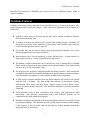
Introduction
1
Background
1
ProShake Features
2
Program Structure
3
Installing ProShake
5
Tutorial
6
Utilities
13
ProShake Help
15
The ProShake Interface
16
Input Manager
16
Solution Manager
26
Output Manager
26
Report
30
ProShake Graphics
32
Theory
33
Verification
41
Strong Motion Parameters
46
Built-In Soil Models
48
Definitions
50
References
52
iii
ProShake User's Manual
Introduction
Welcome to ProShake, a new computer program for seismic ground response analysis of
horizontally layered soil deposits. ProShake was developed from EduShake, a public domain
program developed to help engineering students understand the mechanics of seismic ground
response. ProShake features a Windows graphical user interface that both simplifies and speeds
the analysis and interpretation of seismic ground response.
If you have used EduShake, you will find that ProShake is virtually identical, except that the
restrictions that prevent EduShake from being used for general problems are removed. If you are
an experienced user of SHAKE (or SHAKE85 or SHAKE91), you will find that ProShake allows
you to input and check data faster and more easily, perform analyses more quickly, and interpret
your results much more easily and efficiently than previous versions of SHAKE. If you are new
to ground response analysis, you will find the intuitive interface of ProShake easy to learn and
use.
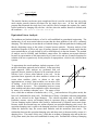
Background
ProShake evolved from an attempt to provide a user-friendly interface to SHAKE for
geotechnical earthquake engineering students. Many current students have only been exposed to
C or other programming languages, and are not familiar with FORTRAN and its formatting
conventions. When first using SHAKE, therefore, they often encounter difficulties in preparing
their input (getting the right number in the right column) and reformatting their output (to put it in
a form that spreadsheets or graphics programs can recognize). As a result, many students spend
more time worrying about input and output than they do learning about ground response.
Initially, a relatively simple system consisting of a front end (preprocessor) and back end
(postprocessor) for SHAKE91 was envisioned. As the programming effort proceeded, however,
it became clear that much greater capabilities could be achieved by developing a single, integrated
program. At that point, the computational portion of the program was written from scratch (in
FORTRAN) and the interface developed (in Visual Basic). As the program began to take shape,
it’s potential benefits to practicing engineers became apparent. At that point, two versions of the
program were developed - EduShake and ProShake. EduShake fulfills the original goal of the
developers - it is a full-featured program that is available at no cost to students, faculty, and other
interested parties. EduShake is limited, however, to the use of only two input motions; this is
sufficient for well-constructed assignments to provide students with a good understanding of
seismic ground response, but not sufficient to allow the program to be used for commercial
purposes.
The development of EduShake evolved through several stages and was eventually beta tested by
graduate students, researchers, and practicing engineers. After a few modifications in response to
the comments of the beta testers, EduShake was made available in the public domain. Shortly
1
ProShake User's Manual
thereafter, the restrictions of EduShake were removed and a few additional features added to
produce ProShake.
ProShake Features
ProShake offers many features that make it easy and efficient to use - features not found in other
ground response analysis software packages. Some of the most significant of these features are
listed below:
•
•
•
•
•
•
•
•
•
English or metric units can be used, and the units can be entered in whatever format is
most convenient during input.
A number of built-in soil models can be selected from pulldown menus. ProShake will
interpolate as necessary to the conditions of your analysis, and will allow you to add your
own soil models and store them for later use.
Soil profile data can be entered quickly using drag-and-drop techniques, and can be
checked graphically for errors prior to analysis.
Input motions can be viewed graphically in many different ways - as time histories, as
spectra, and in terms of a variety of ground motion parameters.
The number of input motions that can be analyzed at a time is limited only by available
RAM, and the results from all input motions can be plotted together. Each input motion
can have up to 16,384 acceleration values.
The progress of the program is displayed graphically during execution. Plots showing the
variation of shear strain and modulus/damping errors during iteration toward convergence
can help illustrate site response as well as identify possible errors in input data.
A wide variety of output parameters from any depth within the soil profile can be plotted
with the click of a button. The plots include time histories of acceleration, velocity,
displacement, shear stress, and shear strain; response spectra, Fourier spectra, power
spectra, and phase spectra; and plots of the maximum amplitudes of various parameters
with depth.
Scalar parameters such as peak acceleration, peak velocity, peak displacement, RMS
acceleration, Arias Intensity, predominant period, and bracketed duration can be
computed for any depth within the soil profile.
ProShake can display an animation of the horizontal displacements of a soil profile excited
by earthquake shaking. The animation provides greatly improved intuitive understanding
of the response of the soil profile, and can help the user identify potential hazards that
might otherwise go undetected.
2
ProShake User's Manual
•
ProShake has a built-in word processor that is linked to the program in a way that allows
analyses to be documented thoroughly and easily in a ProShake Report. The ProShake
Report can include text, tables, and graphics - all of which can be cut-and-pasted into
more powerful word processors for final report preparation.
These are only some of the features that ProShake offers to simplify and speed the process of
performing and interpreting the results of ground response analyses. As you become more
familiar with the program, other helpful features will become apparent.
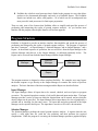
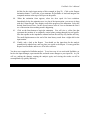
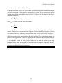
Program Structure
ProShake is designed to provide an intuitive interface that simplifies and speeds the process of
performing and interpreting the results of ground response analyses. The program is organized
into three “managers” - an Input Manager, a Solution Manager, and an Output Manager - and a
Report. In the normal sequence of operations, the user will move from the Input Manager to the
Solution Manager and then on to the Output Manager, as indicated graphically below. The
Report can be accessed from both the Input Manager and the Output Manager.
Input
Manager
Solution
Manager
Output
Manager
Report
The program structure is designed to allow complete flexibility. For example, users may bypass
the normal sequence to go directly to the Output Manager to examine the results of previous
analyses. The basic functions of the three managers and the Report are described below.
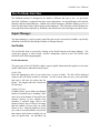
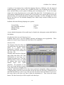
Input Manager
The Input Manager allows all input data to be entered, checked, and saved prior to program
execution. The required input data consists of soil profile data and input motion data. The Input
Manager provides a series of forms on which the required data can be entered, and on which the
desired output can be specified. The Input Manager allows input data to be viewed graphically, a
valuable aid in checking for data entry errors. All input data and plots generated in the Input
Manager can be copied to the Report. The input data is saved in a file with a .dat extension.
Solution Manager
The Solution Manager performs the actual ground response analysis. It requires that the user
specify a valid input data file (with the .dat extension) and then performs the required
computations. While the program is executing, the Solution Manager presents a graphical display
3
ProShake User's Manual
that allows the user to track the progress of the analysis. Upon completion of the analysis, the
Solution Manager saves the results in a file with a .lyr extension.
Output Manager
The Output Manager allows the user to generate a wide range of plots of the results of the
analysis. It requires that the user specify a valid output data file (with the .lyr extension), and then
provides a number of forms for plotting time histories, spectra, variations of parameters with
depth, and for computation of scalar parameters. The Output Manager also allows the user to
view an animation of the horizontal displacements throughout the soil profile - many users find
this feature very helpful for developing an intuitive understanding of the response of the soil
profile. All plots generated in the Output Manager can be copied to the Report.
Report
The Report produced by a word processor that is built into ProShake. The Report allows the
user to keep a record of each analysis. All input data is automatically written to the Report and
updated when the Report is accessed. All plots generated in the Input Manager and Output
Manager can be copied to the Report and saved in a format that can be read by other, more
powerful word processors. Many users find the Report useful for internal documentation of their
analyses, and for preparation of project reports for their clients.
4
ProShake User's Manual
Installing ProShake
The first step in using ProShake is to install the program. ProShake comes on two 3.5” disks,
labelled Disk 1 and Disk 2, and with a hardware key that fits into the parallel port of your
computer. The hardware key will protect your investment in ProShake by preventing
unauthorized use or copying of the program. In order to run ProShake, the hardware key must be
installed on your computer. The hardware key is otherwise transparent to the computer; if you
are already using the parallel port for a particular device, you may insert the hardware key in the
parallel port and plug your device into the other end of the hardware key.
ProShake runs under the Windows 95 or NT 4.0 operating system - it will not run under earlier
versions of Windows (e.g. Windows 3.1). To install ProShake:
1.
2.
3.
4.
5.
Start your computer.
Start the Windows 95 operating system.
Place ProShake Disk 1 in the a:\ drive.
Click on the Windows 95 Start button and select Run.
Type the following in the command line:
a:\setup.exe
and click on OK.
6. Follow the instructions on the screen.
ProShake will be installed in a directory called ProShake (unless you specify otherwise). An
Uninstall program will also be installed in that directory in the event that you need to remove
ProShake from your computer. After installation, ProShake can be accessed using the Windows
95 Start button (then to Programs and on to ProShake).
5
ProShake User's Manual
Tutorial
The easiest way to learn the basics of ProShake’s organization and operation is to complete the
tutorial exercise detailed in this section. The tutorial will take you through nearly all of
ProShake’s functions; it should take you about 20 minutes to complete.
The first step in the tutorial exercise is to start the ProShake program. Click on the Windows 95
Start button, move to Programs, to ProShake, and then click on the ProShake icon to start the
program. After it has started, you can work your way through the tutorial.
The first screen ProShake displays shows the ProShake symbol and six menus - (from left to
right) Input Manager, Solution Manager, Output Manager, Utilities, Help, and Exit. Let's look at
the last three first.
ProShake includes two utilities. One allows you to add new modulus reduction and damping
curves or to modify existing curves. These can be useful when the library of built-in modulus
reduction and damping curves are not appropriate for one or more of the soil types you need to
analyze. The other allows you to convert digitized earthquake records to ProShake format. Use
of these utilities is described later in the User’s Manual.
ProShake has an extensive help system that operates like most conventional Windows help
systems, and can be accessed in two ways. First, clicking on the Help menu will allow you to
choose between working your way through the contents of the ProShake help system and
searching for the specific item you are interested in. The second way of accessing the help system
is through its context-sensitive capability - simply move the cursor to the field you want
information for, then press F1.
The Exit command is self-explanatory - clicking on it will end the program.
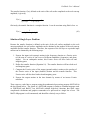
Setting Up an Analysis
Setting up a ProShake analysis involves defining the properties of all soil layers within the profile
to be analyzed, specifying the characteristics of the input motion that will be applied to the soil
profile, defining the quantities to be computed, and documenting the input data. Follow the steps
in the following sections to set up, run, and view the results of a typical ground response analysis.
6
ProShake User’s Manual
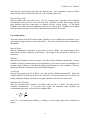
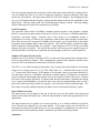
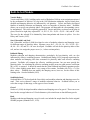
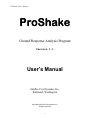
50 ft
50 ft
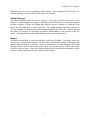
Soft silty clay
γ sat = 100 pcf
vs = 150 m/sec
PI = 10
Stiff clay
γ sat = 120 pcf
G max = 1,800 ksf
PI = 20
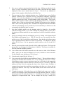
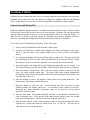
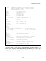
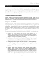
The tutorial will set up and solve for
the response of the soil profile shown
to the left when subjected to a bedrock
motion equal to that recorded at Yerba
Buena Island in the 1989 Loma Prieta
earthquake. The soil profile consists of
a 50 ft thick layer of soft silty clay over
a 50 ft thick layer of stiff clay underlain
by bedrock. The groundwater level is
at the ground surface. The input
motion is to be applied at the top of
bedrock.
The tutorial will take you through the
main steps in a typical ProShake
analysis - definition of layer properties,
Bedrock
specification
of
input
motion,
γ = 150 pcf
documentation
of
input,
running
the
vs = 2,500 ft/sec
analysis, and documenting the results
of the analysis. Each of these steps are
described in detail in the following sections. Completion of the tutorial will provide a very good
introduction to the structure and operation of ProShake.
Definition of Layer Properties
1.
Select the Input Manager from the initial ProShake screen. This will bring up a form
that allows you to define a soil profile, select an input motion, and keep a record of your
input data in a report. If you wanted to open an existing input file, you could do so
under the File menu on this screen (there is an input file named shake.dat that you may
want to look at when you've completed this tutorial - it contains the example soil profile
used in the original SHAKE user's manual).
2.
Type in a title for the soil profile. This title should identify the soil profile to you and
other potential users - it will be echoed on subsequent screens and in output files. Hit
the Tab key after entering the title to automatically move the cursor to the next field, or
move to the next field using the mouse.
3.
Enter the number of layers for the analysis. For this example, enter 16 (then hit Tab) this will provide 15 soil layers plus the underlying halfspace. Note how ProShake
provides 16 tabs when the number of layers is entered - each tab will allow you to input
the appropriate data for the corresponding layer.
4.
Enter the depth of the groundwater table. Because ProShake performs total stress
analyses, the groundwater table depth is not needed for the ground response analysis rather, it is used when vertical effective stresses need to be computed. For this example,
enter 0.0 in either the ft or m box (the other will automatically be calculated). ProShake
allows you to enter input data in either US or SI units, and to mix and match units.
7
ProShake User's Manual
5.
Now you are ready to enter input data for the first layer. Making sure that the tab for
Layer 1 is active (it should be at the front of the stack of tabs with the layer number
displayed in blue), enter a material name for Layer 1. This can be any alphanumeric
string - for this example, call the first layer Soft Silty Clay.
6.
The next step is to select a modulus reduction curve. ProShake has a series of built-in
modulus reduction curves extracted from the geotechnical earthquake engineering
literature. To see the list of built-in curves, click on the button at the right side of the
modulus reduction curve field. For this example, select Vucetic-Dobry. The VuceticDobry model describes modulus reduction (and damping) behavior as a function of
plasticity index. When you select this model, ProShake will prompt you for a plasticity
index - enter 10 for the plasticity index. ProShake will interpolate between the modulus
reduction (and damping) curves presented by Vucetic and Dobry to obtain curves that
correspond to the plasticity index you enter.
7.
Note that ProShake initially sets the damping model as identical to the modulus
reduction model by default. If you want to change the damping model, you may do so
by selecting a different model in the same manner used to select the modulus reduction
model.
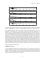
8.
Check your modulus reduction and damping curves by clicking on the button labeled
Plot Modulus and Damping Curves. This will show the curves you specified in yellow
and the curves of the Vucetic-Dobry model in green. Note that the two left-most green
curves represent plasticity indices of 0 and 15, respectively. You should see that the
yellow (PI=10) curve is in the appropriate position relative to the PI=0 and PI=15
curves.
9.
Place the cursor anywhere on the plot and click the right mouse button. The forms that
pop up allow you to change the characteristics of the plot. This feature is available for
all of the plots that ProShake generates.
10.
Now return to the Soil Profile form and move the cursor to either of the Thickness
fields - again, you can enter the thickness in ft or in m, whichever is more convenient.
For this example, enter a thickness of 5 ft for Layer 1.
11.
Enter the unit weight (100 pcf) for Layer 1.
12.
Now you need to specify the low-strain stiffness of Layer 1. This can be done either by
entering the maximum shear modulus, Gmax, or by entering the shear wave velocity.
Using whatever units are most convenient, enter one or the other in the appropriate
field. For this example, enter the shear wave velocity of Layer 1 (150 m/sec). Note that
striking the Enter key after entering the shear wave velocity causes ProShake to
compute the maximum shear modulus corresponding to the shear wave velocity and unit
weight of the material. Now Layer 1 has been defined, and it is time to move on to the
other layers.
13.
Though the properties of the other layers can be defined in the same way, it will be
faster for our example to enter subsequent data using the Summary Data tab. Click on
that tab (just to the left of the tab for Layer 1). You will then see the Layer 1 input data
displayed in a compact tabular form. For our example, the silty clay is actually 50 ft
8
ProShake User’s Manual
thick and we will represent it in our ProShake analysis by ten 5-ft-thick layers. Rather
than type all of this data in 10 times, we will use the drag-and-drop feature of the
Summary Data form. To do this, put the cursor anywhere within the area that defines
Layer 1 on the Summary Data form. Press and hold the left mouse button, then move
the cursor down to the area that defines Layer 2. Release the mouse button and you will
see that all of the data from Layer 1 has been assigned to Layer 2. Now repeat this
process to define the properties of Layers 3-10.
14.
For our example, the silty clay layer is underlain by 50 ft of very stiff clay which we will
represent using five 10-ft-thick layers. To enter the data for Layer 11, first copy the
properties of Layer 10 to Layer 11 by dragging and dropping. Now change the
thickness of Layer 11 from 5 ft to 10 ft - click on the thickness cell for Layer 11 and
type 10 followed by the Tab key. Using the same procedure, change the material name
to Stiff Clay, the unit weight to 120 pcf, Gmax to 1,800 ksf, and the modulus and
damping parameters to 20 (indicating PI=20).
15.
Now use the drag-and-drop feature to copy the properties of Layer 11 to Layers 12
through 15.
16.
Finally, the properties of the half-space (bedrock) must be specified. Working either on
the Summary Data form or on the tab for Layer 16, enter the input properties for
bedrock with a unit weight of 150 pcf and shear wave velocity of 2500 ft/sec. Assign
the Rock modulus reduction and damping curves to Layer 16.
17.
Now we must specify what information is to be computed during the ground response
analysis. Go to the tab for Layer 1 and click on the Select Output button. On the form
that appears, check the boxes for acceleration and velocity. Also, check the box for
acceleration response spectrum and enter damping ratios of 5, 10, and 20%. Repeat this
process for Layers 2 and 11, but now requesting plots of shear strain and shear stress for
those layers.
18.
Now that all of the layers are defined, check for obvious errors (such as a misplaced
decimal point) by clicking the View Profile button. The profile shows the variation of
unit weight and shear wave velocity with depth - our example shows significant
impedance (product of shear wave velocity and density) contrasts at the boundaries
between the silty clay and the stiff clay (at the bottom of Layer 10) and between the stiff
clay and bedrock (bottom of Layer 15). As we will see, these impedance contrasts will
have a strong influence on the seismic response of our soil profile. The locations at
which output is to be computed are indicated by green ovals - you should see these at
the tops of Layers 1, 2, and 11.
Specification of Input Motion
19.
Now the input motion must be specified. Click on the large Input Motion button on the
main Input Manager form. This will bring up a form that allows you to select an input
motion, define its characteristics, view it graphically, and compute various ground
motion parameters associated with the motion.
9
ProShake User's Manual
20.
Enter 1 for the number of motions. ProShake allows you to analyze a soil profile using
many different input motions in an individual run. For this example, leave the strain
ratio, maximum number of iterations, and error tolerance at their default values.
21.
Click the Open button on the tab form for Motion 1. From the Open File menu that
appears, select the file named "yerba.eq." This file contains a strong motion record
obtained at a rock outcrop on Yerba Buena Island in San Francisco Bay during the 1989
Loma Prieta earthquake. The characteristics of the record will be displayed in the
Object Motion box (the peak acceleration, time step, and cutoff frequency can be
changed, if desired). Various plots and common ground motion parameters for the
object motion can be obtained by clicking on the buttons at the right side of this form you should spend a little time playing with these.
22.
Assign the object motion to the top of bedrock by entering 16 in the Layer field within
the Object Motion Location box. Specify this motion as an outcrop motion by checking
the appropriate box.
23.
Select "Yes" in the Animation box. This will instruct ProShake to compute the
response at the locations necessary to produce an animated view of ground response
that can be viewed in the Output Manager.
24.
The soil profile and input motion have now been completely characterized. Save the
input data file with the name "tutorial.dat."
Documentation of Input
25.
Click on the large Report button on the main Input Manager form. This will open a
dedicated word processor with a template that shows all of the input data in tabular
form. The report can be printed directly from ProShake, or saved (in Rich Text Format)
for subsequent editing using a more powerful word processor.
26.
Graphics can also be copied to the report. Go back to the Input Motion form and plot
the time history of acceleration of the input motion. Click the button labeled Copy to
Report, and then go back to the Report. You should see that the input motion has been
copied to the report at whatever location the report cursor was in. Any ProShake plot
can be copied to the report to provide documentation of a ground response analysis.
27.
Now, save the report with the name "tutorial.hed."
Running the Analysis
28.
To run the ProShake analysis, select the Solution Manager.
29.
The Solution Manager will analyze any input data file you desire. The default extension
for ProShake input files is .dat, though other filename extensions can also be used. To
run the analysis you have just set up, select the data file tutorial.dat.
10
ProShake User’s Manual
30.
ProShake will then perform the analysis. You will see how the program iterates toward
strain-compatible soil properties during the analysis - this feature will help you develop a
better understanding of the response of your soil deposit. The word "Running" will
appear in the lower left corner of the screen, and will be replaced by the word "Finished"
at completion of the analysis and a dialog box will appear. When the analysis is
completed, click OK on the dialog box that appears to exit Solution Manager. The
results of the analysis performed by the Solution Manager will automatically be written
to a file with the same name as your data file, but with the extension .lyr - in this case
tutorial.lyr.
Examining the Results of the Analysis
31.
To view the results of your analysis, select the Output Manager.
32.
Go to the File menu in the Output Manager and open the file tutorial.lyr.
33.
There are many options for viewing the results of your analysis in the Output Manager.
The primary plot types are organized on a series of six tabs - Ground Motion Plots,
Stress and Strain Plots, Response Spectrum Plots, Depth Plots, Other Parameters, and
Animation.
34.
The Ground Motion Plots form allows you to plot time histories and Fourier spectra at
the tops of the layers you selected in Step 17 of the tutorial. You may plot one or more
motions on the same graph by checking the desired boxes. Go ahead and create a
couple plots of your output. Note that these plots can be copied to the Report from the
Output Manager just as they could from the Input Manager.
35.
The Stress and Strain Plots form allows plotting of time histories and spectra of shear
stress and shear strain - for our example, plots should be available at the tops of Layers
2 and 11.
36.
The Response Spectrum Plots form allows you to plot any or all of the response spectra
that you requested in Step 17. For this example, ground surface response spectra with
5%, 10%, and 20% damping were requested - select them all and plot them on the same
graph, then copy the graph to the Report.
37.
The Depth Plots form can be used to plot the variation of several quantities with depth
for one or more input motions. Since our analysis used only one input motion, check
the box for Motion 1 and try plotting some of these quantities with depth.
38.
The Other Parameters form offers the opportunity to compute a variety of useful
ground motion parameters at the tops of any of the layers selected in Step 17. Highlight
the layer you are interested in, and then click on the Calculate button to see the
numerical values of the parameters. This information can be copied in tabular format to
the Report.
39.
Finally, the Animation form allows you to view the variation of horizontal displacements
with both depth and time for each input motion that an animation was requested for (you
11
ProShake User's Manual
did this for the single input motion of this example in Step 23). Click on the Prepare
Animation button - it will take a few moments for ProShake to load and integrate the
computed motions at the tops of all layers in the profile.
40.
When the animation form appears, select the slow speed for best resolution.
Immediately below the animation axes is a plot of the input motion; you can use it along
with the Current Record Time display to track the progress of the animation. Select the
desired Start Record Time - for this record, enter a value of 8 sec to eliminate the first 8
sec of the motion where nothing much is happening.
41.
Click on the Start button to begin the animation. You will view a yellow line that
represents the position of an originally vertical plane passing through your soil profile.
Note the response at the impedance contrast between the soft silty clay and the stiff clay.
The small displacements at the end of the time history result from a slight drift in the
input motion.
42.
Finally, take a look at the Report. You should see the input data for the analysis
summarized in tabular form, and any plots you copied to the Report. You may print the
Report from ProShake and/or save it for later reference.
You have now completed a ProShake analysis. To see how easy it is to work with ProShake, go
back to the Input Manager, open tutorial.dat, and make some changes to your input file. As you
will see, making the changes, running the analysis again, and viewing the results can all be
accomplished very quickly and easily.
12
ProShake User’s Manual
ProShake Utilities
ProShake has two utilities that allow users to reformat digitized ground motions to be used with
ProShake and to input their own soil models by adding new modulus reduction and damping
curves. Both utilities save new data in a form recognizable to ProShake for future analyses.
Convert Ground Motion File
Digitized earthquake ground motions are available from many different sources, and the formats
in which they are provided by those sources are often different. ProShake, like any other ground
response analysis program, expects to see the ground motion values in a particular format. To
allow the user to specify any ground motion as a ProShake input motion, ProShake includes a
utility for converting and saving ground motions in the format required by ProShake.
To use the Convert Ground Motion File utility, follow these steps:
1. Select Convert Ground Motion File from the Utilities menu.
2. An Open File Dialog Box with the title Earthquake File Name will appear on the screen.
Select or enter the name of the ground motion file you wish to convert to ProShake
format.
3. A Convert Ground Motion File form will then appear on the screen. The upper part of the
box will display the first five lines of the ground motion file you plan to convert. Below
that display is a series of text boxes that allow you to specify the format of the file.
4. Specify the name of the output file for the ProShake-formatted file you are creating. You
can use any filename you wish, but ProShake will look first for files with the .eq extension.
5. Enter the number of header lines. This is the total number of lines at the top of the file
before the actual ground motion data. The header lines often contain alphanumeric
descriptions and/or numerical information about the motion (number of data points, time
step, maximum value, etc.).
6. Enter the number of values - the number of data points in the ground motion file. This
information is often shown in the header lines.
7. Enter the number of values per line. Ground motion data files are written in many
different formats, but usually consist of 6 - 8 acceleration values written on each line.
Determine how many individual acceleration values are on each line of your ground
motion file and enter it here.
8. Enter the field width. The ground motion file will allot a certain number of characters for
each acceleration value. Note that the field width includes negative signs, the decimal
point, and any blank spaces. Determine the field width and enter it here.
9. Enter the time interval. Each of the acceleration values in the ground motion file will be
separated by a certain time interval, usually 0.005, 0.01, or 0.02 sec. The time step is
often shown in one of the header lines.
13
ProShake User's Manual
10. Select the units of acceleration in the file you are converting. Choose from fraction of
gravity (g), cm/sec2, m/sec2, in/sec2, or ft/sec2. Most ground motion files will express
accelerations in g’s, but some use other units. Note that 1 gal = 1 cm/sec2.
11. After providing all of the required information, click on OK. ProShake will read your file
and write a new file with the same acceleration data (expressed in g’s) arranged in
ProShake format. Your original file will be unchanged.
Modulus-Damping Curve Editor Utility
ProShake approximates the nonlinear, inelastic behavior of soils using an iterative, equivalent
linear approach. This approach requires that the variation of secant shear modulus and damping
ratio with shear strain be specified. This behavior is described by modulus reduction and damping
curves.
A modulus reduction curve illustrates the variation of normalized secant shear modulus (secant
shear modulus divided by maximum shear modulus, or G/Gmax) with strain. A damping curve
illustrates the variation of equivalent viscous damping ratio with strain. The modulus reduction
and damping behavior of many soils is well understood, and several models have been proposed
to characterize them. ProShake has a number of built-in modulus reduction and damping models,
but users may wish to add new models using the modulus-damping curve editor.
To add a new modulus reduction or damping curve, follow these steps:
1. Select Modulus-Damping Curve Editor from the Utilities Menu. A Modulus-Damping
Curve Library Editor box will appear on the screen displaying modulus and strain values
for Model No. 1 - the Vucetic-Dobry model. Note that there are 6 curves in the VuceticDobry model (each corresponding to a different plasticity index), and that each curve is
defined at 16 different strain levels. Individual modulus reduction values can be changed,
but any changes should be documented (or preferably saved with a different model name).
2. If you want to create a new damping curve, select Damping in the upper box. If not, leave
Modulus selected.
3. Click the Add button. You will now have a blank form on which to enter the modulus
reduction data for your new model.
4. Give the model a name. You may use any alphanumeric name, but make sure that it is
different than the names of the existing models. The length of the name is limited to 50
characters.
5. Enter the number of curves defining your new model. If modulus reduction behavior
depends only on strain level in your model, you will only need one curve. If modulus
reduction behavior depends on a second parameter (e.g. plasticity index in the VuceticDobry model), enter the number of values of that parameter for which modulus reduction
data will be entered (6 in the case of the Vucetic-Dobry model).
14
ProShake User’s Manual
6. Enter an alphanumeric description of the second parameter.
7. Enter the number of points defining each curve; this is equal to the number of strain values
at which modulus reduction ratio is to be specified.
8. If you specified more than one curve (for a model in which modulus reduction behavior
depends on another parameter in addition to strain level), enter the values of that
parameter for which modulus reduction curves are to be entered in each column of the
first row of the data grid.
9. Enter the desired strain values in the left-most column, and the corresponding modulus
reduction ratio values in the appropriate Modulus columns.
10. When the data is entered and you have checked it, click OK.
11. To add additional curves, repeat steps 3 to 10 for each curve.
12. Click Save.The data you have entered will be saved and be available for subsequent use
via the pulldown menu in the Input Manager. The pulldown menu will display the model
name you entered in Step 4 and, if applicable, the parameter name you specified in Step 6.
ProShake Help
ProShake has extensive help capabilities. The ProShake help system follows standard Windows
help file protocol. Each screen that ProShake displays provides access to the Help system
through a pull-down menu. Also, context-sensitive help is available by clicking on the item for
which more information is desired, then pressing the F1 key.
There are two options for navigating through the Help system. The first is initiated by selecting
Contents from the Help menu. This selection will allow you to explore the structure of ProShake
by working your way through the Input Manager, Solution Manager, or Output Manager. Each
selection takes you through the various managers and has explanations for each item on each form
that ProShake displays. The second option for using the Help system is through the use of the
index, activated by selecting ‘Search for Help on’ from the Help menu. The index is particularly
helpful if you know what you’re looking for - either scroll down through the alphabetical list of
help topics or begin typing the name of the item you are looking for. When you have found the
item you want, either double-click on it or highlight it and click on Display.
15
ProShake User's Manual
The ProShake Interface
The ProShake interface is designed to be intuitive, efficient, and easy to use. As previously
described, ProShake is organized into three main components - the Input Manager, the Solution
Manager, and the Output Manager. Within each of these managers, ProShake displays a series of
forms on which data can be entered and/or results displayed. The following sections illustrate the
most significant forms displayed by ProShake, and describes the items that appear on those forms.
Input Manager
The input manager is used to prepare input files that can be executed by ProShake, specifically
definition of the Soil Profile and specification of all Input Motions
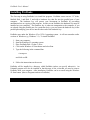
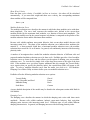
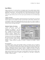
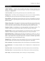
Soil Profile
The Soil Profile form is accessed by clicking on the Profile button in the Input Manager. The
screen that appears is shown below, and the information entered on the Soil Profile form
described in the following paragraphs.
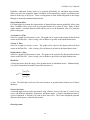
Profile Information
The upper part of the Soil Profile window requests global information that applies to the entire
profile, rather than to individual material layers
Profile Title
Enter the alphanumeric title of your choice here, or leave it blank. The title will be displayed
whenever the Soil Profile window is activated. It will be stored when you save your soil profile
data and it will also be written into the
Report. The length of the title is limited to
80 characters.
Number of Layers
ProShake allows you to define an unlimited
number of material layers, including a halfspace layer at the bottom of the profile (the
memory capacity of your computer may
introduce a practical upper limit to the
number of layers, but it is likely to be larger
than the number of layers that you would
choose to use). Enter the number of layers
you want to use and ProShake will provide
that number of tab forms on which you can
enter soil profile data. An individual soil
16
ProShake User’s Manual
layer may be represented by more than one material layer. As an alternative, users may find it
more efficient to enter material data directly on the Summary Data form.
Depth to Water Table
Enter the depth to the water table, if any. Use U.S. or metric units - the other will be calculated
automatically when you move to the next data field. ProShake uses this depth, along with the
layer thickness and unit weight data, to compute effective vertical stresses. If left blank,
ProShake will assume that no groundwater exists in the entire profile. ProShake will compute
initial porewater pressures as zero above and hydrostatic below the water table.
Layer Information
The main portion of the Soil Profile window contains a series of tabbed forms that allow you to
enter material property data for each material layer. The active material layer form is indicated by
the tab label.
Material Name
Enter the alphanumeric description of your choice, or leave it blank. The material name will be
stored in the Analysis Summary in the Report. The length of the description is limited to 20
characters.
Thickness
Enter the layer thickness in feet or in meters - the other will be calculated automatically. Because
ProShake computes ground motions at layer boundaries, you'll want to select layer thicknesses to
provide a layer boundary at each depth at which ground motions are to be computed. This may
require specification of adjacent layers with identical properties.
Unit Weight
Enter the unit weight in pcf or in kN/m3 - the other will be calculated automatically. Moist unit
weights should be used for layers above the water table. Because porewater moves with the soil
during earthquake shaking, saturated unit weights should be used below the water table.
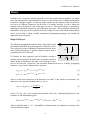
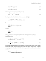
Maximum Shear Modulus
Enter the maximum shear modulus, if available, either in ksf or in MPa - the other will be
calculated automatically. If you enter unit weight and maximum shear modulus, the
corresponding shear wave velocity will be computed from
vs = G ρ =
Gg
γ
where Gmax is maximum shear modulus, ρ is density, γ is unit weight, and g is the acceleration of
gravity.
17
ProShake User's Manual
Shear Wave Velocity
Enter the shear wave velocity, if available, in ft/sec or in m/sec - the other will be calculated
automatically. If you enter unit weight and shear wave velocity, the corresponding maximum
shear modulus will be computed from
Gmax = ρ v2
s
Modulus Reduction Curve
The modulus reduction curve describes the manner in which the shear modulus varies with shear
strain amplitude. The curve itself expresses the modulus ratio, defined as the secant shear
modulus divided by the maximum shear modulus, as a function of shear strain amplitude. The
secant shear modulus used in the ground response calculations is computed as the product of the
modulus reduction factor and the maximum shear modulus.
Because soils exhibit nonlinear stress-strain behavior, their secant shear moduli decrease with
increasing strain level. The shape of the modulus reduction curve indicates how nonlinear the
material is - a linear material would have a horizontal modulus reduction curve; the modulus
reduction factor would be 1.0 at all strains. In general, soil nonlinearity increases with decreasing
plasticity index.
A number of investigators have studied the modulus reduction behavior of different soils and
proposed standard modulus reduction curves for those soils. ProShake provides a list of modulus
reduction curves to choose from, and also allows you the option of defining your own modulus
reduction curve. To view the list, simply click on the drop-down arrow to the right of the data
field. If the modulus curve you select requires additional data (for example, the Vucetic-Dobry
curve requires that you specify the plasticity index), the required data fields will appear to the
right. To select a modulus reduction curve from the menu, just click on it. See ModulusDamping Curve Editor Utility section to define your own modulus reduction curve.
ProShake offers the following modulus reduction curve options:
Vucetic-Dobry
Sun, Golesorkhi, and Seed
Ishibashi-Zhang
Seed-Idriss
Gravel
Linear
Rock
Custom
A more detailed description of the models may be found in the subsequent section titled Built-In
Soil Models.
Damping Curve
The damping curve describes the manner in which the damping ratio varies with shear strain
amplitude. Because soils exhibit nonlinear, inelastic stress-strain behavior, their equivalent
damping ratios increase with increasing strain level. Different types of soil exhibit different
damping characteristics. In general, soil damping increases with decreasing plasticity index.
18
ProShake User’s Manual
A number of investigators have studied the damping behavior of different soils and proposed
standard damping curves for those soils. ProShake provides a list of damping curves to choose
from, and also allows you the option of defining your own damping curve. To view the menu,
simply click on the drop-down arrow to the right of the data field. If the damping curve you
select requires additional data (for example, the Vucetic-Dobry curve requires that you specity the
plasticity index), the required data boxes will appear to the right. To select a damping curve from
the list, just click on it. See Modulus-Damping Curve Editor Utility section to define your own
damping curve.
ProShake offers the following damping curve options:
Vucetic-Dobry
Sun, Golesorkhi, and Seed
Ishibashi-Zhang
Seed-Idriss
Constant
Rock
Custom
A more detailed description of the models may be found in the subsequent section titled Built-In
Soil Models.
Plot Modulus Reduction and Damping Curves
ProShake allows you to view the modulus reduction and damping curves graphically. These
graphs also feature Copy to Report and Write Data to File capabilities.
Summary Data
The Summary Data form allows the
soil profile data to be entered and/or
edited in a tabular format.
Experienced ProShake users may
find this format more efficient for
data entry. The
Summary Data form has a drag-anddrop feature that allows all of the
characteristics of one layer to be
assigned to another layer. The dragand-drop feature can be very useful
for entering data when multiple
material
layers
have
similar
properties - the properties of one
layer can be input and then assigned
to the other layers by dragging and
dropping. Individual properties of the other layers can then be changed by editing as necessary.
To drag-and-drop, place the cursor anywhere on the line (data for each layer is displayed on an
individual line) that you want to copy, then press the left mouse button and hold it as you move
the cursor down to the layer you want to paste the information to. Then, release the mouse
button. The data for one layer will be copied to the other layer.
19
ProShake User's Manual
Select Ouput
Output can be requested for the top of any soil layer in the profile prior to program execution.
Output is divided into three main categories that are displayed on the Select Output form:
Time History
Time histories of acceleration, velocity, displacement, shear strain, and shear stress can be
selected for any layer. The exception is that shear stress and shear strain cannot be selected for
Layer 1 because their values are always zero at the ground surface.
Response Spectrum
Acceleration, velocity, and/or displacement response spectra can be computed at up to three
structural damping ratios. Response spectra are computed at 95 structural periods ranging
from 0 to 10 seconds.
Spectra
Fourier spectra, phase spectra, and power spectra can be computed for acceleration, velocity,
and/or displacement.
View Profile
ProShake’s Input Graphics allow you to view the soil profile and input parameters assigned to
various material layers. This feature is very useful for detecting errors or other problems with the
input data - mis-typed parameters or misplaced decimal points will show up very clearly in the
profile.
The profile shows the name,
thickness, unit weight, and shear
wave velocity for each material
layer. The profile indicates the
depths at which the input motions
are applied (with solid red ovals for
motions within the profile and open
ovals for outcrop motions) and the
depths at which output is calculated
(with solid green ovals for motions
within the profile and open ovals
for outcrop motions). The profile
plot can be copied to the Report.
The profile is also useful for
visualizing impedance contrasts at layer boundaries. Because impedance ratios control the
partitioning of wave energy (reflected and transmitted) at layer boundaries, it is useful to know
where the highest impedance ratios are located.
20
ProShake User’s Manual
Input Motion
Proper specification of an input motion is an important part of any ground response analysis.
ProShake allows you to view a variety of potential input motions and select the ones that are most
appropriate for the analysis. The selection and review of input motions takes place on the Input
Motion form. The upper part of the Input Motion form requests global information that applies
to all of the input motions you select; the lower part requests information for each individual input
motion.
Number of Motions
ProShake places no limit on the number of input motions that can be specified for a given run (the
memory capacity of your computer will place a practical limit on the number of motions, but it
will generally be larger than the number that most users will wish to use). Enter the number of
input motions you want to use and ProShake will provide that number of tab forms on which you
can select and/or enter input motion data.
Maximum Number of Iterations
ProShake approximates nonlinear soil
behavior by iterating toward straincompatible soil properties.
You can
specify the maximum number of iterations
here - ProShake will continue until it
reaches this limit or until the tolerance
criterion is satisfied. ProShake uses a
procedure to adjust the soil properties that
converges more quickly and reliably than
that used in previous versions of SHAKE.
For most soil profiles, strain-compatible
properties will be reached in a few
iterations. During execution, the number of iterations is displayed by ProShake’s Solution
Graphics.
Error Tolerance
As ProShake iterates toward strain-compatible modulus and damping values, the difference
between the modulus and damping values from one iteration to the next becomes smaller and
smaller. You can specify any error tolerance defined as the maximum percentage change in shear
modulus or damping ratio between successive iterations. ProShake will iterate toward straincompatible soil properties until the tolerance criterion is satisfied for all layers or until the
maximum number of iterations is reached. The results of many ground response analyses do not
change much at tolerance levels below about 5% and ProShake will use this as a default value.
During execution, the variation of modulus and damping error with depth is illustrated by
ProShake’s Solution Graphics.
21
ProShake User's Manual
Strain Ratio
The strain ratio is the ratio of effective shear strain to maximum shear strain in each layer.
ProShake takes transient input motions and computes transient output motions. The computed
shear strain is an important output parameter because of the strain-dependence of the shear
modulus and damping ratio. The process of iteration toward strain-compatible modulus and
damping values requires comparison of the strains computed in each iteration of ProShake with
the strains on which the modulus and damping values are based. Because equivalent linear
modulus and damping characteristics are based on laboratory tests with uniform harmonic
loading, the transient shear strain computed by ProShake must be converted to an effective shear
strain for this comparison. Historically, the strain ratio has often been taken as 0.65, but can
better be selected as (M-1)/10 where M is the magnitude of the earthquake that produced the
input motion.
Object Motion
An object motion is an input motion read from a data file and assigned to a particular layer
boundary in the soil profile. ProShake computes the response at other points in the soil profile to
the object motion. In this section you will select and specify the characteristics of each individual
input motion.
File Name, Open, Remove
Enter the complete name of the input motion file here, or use the Open command button to
browse through all Windows 95 directories.
Description
Enter the alphanumeric description of your choice here. This description will be attached to all
pertinent data and graphics copied to the Report or written to your Data File. The length of the
description is limited to 128 characters.
Number of Acceleration Values
ProShake uses digitized earthquake records. This term indicates the number of acceleration
values in the current input file. The number of acceleration values in a ProShake earthquake
record cannot exceed 16,384.
Peak Acceleration
The maximum (absolute) acceleration of the current input file is displayed here. You can change
this value if you want to scale the accelerations to a different maximum acceleration for your
analysis - the input motion data file will not be changed. By changing the maximum acceleration,
you will change all acceleration values in the input motion by the same factor. The frequency
content and duration of the input motion will not be affected by amplitude scaling.
Time Step
22
ProShake User’s Manual
The time step that separates the acceleration values in the input motion data file is displayed here.
You can change this value if you want to change the frequency content or duration of the input
motion for your analysis - the input motion data file will not be changed. By changing the time
step, you will change both the frequency content and the duration (but not the amplitude) of the
input motion. This is a rather crude way of modifying the frequency content - time step changes
of more than about 20% should be considered very carefully.
Cutoff Frequency
The equivalent linear mode of ProShake computes ground response in the frequency domain.
Briefly, it represents an input motion as the sum of a series of sine waves of different amplitudes,
frequencies, and phase angles. Because most of the energy in an earthquake motion is
concentrated in a range of relatively low frequencies (and because high frequency motions have
little effect on most civil structures), ProShake doesn't require you to spend time on the higher
frequencies that contribute little to the total response. The cutoff frequency specifies the upper
limit of frequencies that ProShake will consider - cutoff frequencies of 15 to 20 Hz are usually
adequate for most soil profiles. The speed of the analysis will increase as the cutoff frequency is
decreased, but the execution time is generally not long enough to justify low cutoff frequencies.
Number of Terms in Fourier Series
ProShake uses a Fast Fourier Transform (FFT) to convert the input motion (time domain) into a
Fourier series (frequency domain). After computing the response in the frequency domain, it uses
an inverse FFT to transform the solution back to the time domain.
The FFT is a very efficient numerical procedure, but it requires the total number of acceleration
values to be an integer power of 2 (e.g. 1024, 2048, 4096, etc.). ProShake allows up to 16,384
(=214) terms in the object motion. If the number of acceleration values in your input motion file is
less than some power of 2, ProShake will add the required number of trailing zero acceleration
values to bring the total length to the number of terms you specify for the Fourier series. Because
the Fourier series implies periodicity (it assumes that the total time history, including the trailing
zeros, repeats itself indefinitely), you need to make sure you have enough trailing zeros to form a
quiet zone sufficiently long to allow the response to die out before the next motion begins. The
best results are usually obtained when the last third or more of the total time history is quiet.
Object Motion Location
The input motion can be applied at the top of any layer in your soil profile, from the ground
surface to the bottom half-space layer. Enter the layer number at which your input motion is to be
applied here.
The input motion may be applied as an outcrop motion or as a motion within the soil profile.
Your selection here depends on your input motion. If the input motion was recorded by an
instrument located on the ground surface, or if it was obtained by computation at a point on the
ground surface of some numerical model, it should be specified as an outcrop motion.
Animation
23
ProShake User's Manual
ProShake’s animation feature needs to be selected individually for individual input motions.
When you select the animation feature, ProShake will automatically compute acceleration time
histories at the tops of all layers. These accelerograms are then double-integrated in the Output
Manager to obtain the animated displacements.
Object Motion Plots
It is often helpful to examine the characteristics of potential input motions graphically before using
them. ProShake allows you to look at your input motions in a variety of ways. Many of these
graphs include a crosshair function which allows you to see the numerical value of a particular
point on the graph.
Acceleration vs Time
Select for a graph of acceleration vs time. The graph can be copied to the Report and/or the data
written to the Data File. After viewing, click on Return to go back to the Input Motion form.
Velocity vs Time
Select for a graph of velocity vs time. The graph can be copied to the Report and/or the data
written to the Data File. After viewing, click on Return to get back to the Input Motion form.
Displacement vs Time
Select for a graph of displacement vs time. The graph can be copied to the Report and/or the data
written to the Data File. After viewing, click on Return to get back to the Input Motion form.
Husid Plot
A Husid plot shows how the energy of the ground motion is distributed in time. Mathematically,
it is a plot of normalized cumulative squared acceleration, i.e.
t
2
∫ [a (t )] dt
H n (t ) =
0
∞
2
∫ [a (t )] dt
0
vs time. The Husid plot can be used for some measures of ground motion duration (see Trifunac
duration).
Fourier Spectrum
A transient input motion can be represented, using a Fourier series, as the sum of a series of sine
waves with different amplitudes, frequencies, and phase angles. A Fourier amplitude spectrum is
a plot of amplitude vs frequency for each of these sine waves. The Fourier amplitude spectrum
illustrates the frequency content of the motion.
Phase Spectrum
24
ProShake User’s Manual
A phase spectrum is a plot of phase angle vs frequency for all of the sine waves that make up a
Fourier series. The phase spectrum controls the manner in which ground motion energy is
distributed in time; the overall shape of a time history is related to the phase spectrum. Unlike
Fourier spectra, phase spectra have no discernible structure.
Power Spectrum
A power spectrum shows how the power of a ground motion signal is distributed with respect to
frequency. The power spectrum really provides the same information as the Fourier spectrum - its
values are the squares of the values of the Fourier spectrum.
Response Spectrum
A response spectrum presents the maximum absolute response (acceleration, velocity, or
displacement) of single-degree-of-freedom oscillators of different natural periods. As such, it
gives a good indication of the potential effects of the ground motion on different structures. For
object motion response spectra, ProShake assumes 5% structural damping.
Crosshairs
ProShake screen graphs include a crosshair feature that allows you to identify the coordinates of
any point on the graph. By moving the cursor onto the graph, the arrow turns into a set of
crosshairs. The coordinates of the center of the crosshairs is given in the Crosshair Position box.
The x- and y-coordinates are those on the horizontal and vertical axes of the graph, respectively,
and the units are the same as those of the graph.
Other Parameters
ProShake will allow you to compute other characteristics of an input motion. Clicking on this
button allows you to compute any of the following ground motion parameters.
Peak Acceleration
Peak Velocity
Peak Displacement
RMS Acceleration
Arias Intensity
Response Spectrum Intensity
Predominant Period
Bracketed Duration
Trifunac Duration
25
ProShake User's Manual
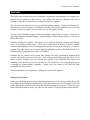
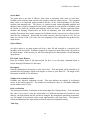
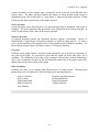
Solution Manager
The solution manager is used to execute the equivalent linear analysis of ProShake. The user
must select a valid ProShake data file for execution. The solution manager will save the selected
output in a file with a .lyr filename extension, e.g. PSRUN.lyr upon execution of the data file
PSRUN.dat.
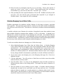
The solution manager will display solution
graphics during execution of the
equivalent linear analysis. The solution
graphics will display three plots for each
input motion. The leftmost plot will
illustrate the variation of effective shear
strain with depth for each iteration - the
effective shear strain values should
converge to a constant profile with
increasing numbers of iterations. The
center and rightmost plots illustrate the
variation of modulus error and damping
error with depth for each iteration. As the
program iterates toward strain-compatible
soil properties, the errors should decrease. When the errors decrease below the error tolerance
specified on the Input Motion form of the Input Manager at all depths, or when the maximum
number of iterations has been reached, the program will cease iterating.
The solution graphics are intended to help the user better understand the behavior of the soil
deposit being analyzed, and to help identify and correct potential problems with the analysis.
ProShake uses iteration logic that is more advanced than that used in previous versions of
SHAKE; as a result, it converges more quickly and more reliably than previous versions. Soil
profiles with extraordinarily soft layers or extraordinarily high impedance ratios, however, may
converge slowly or not at all - such behavior often indicates an error in the input.
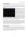
Output Manager
The output manager processes all output and allows all results to be plotted graphically. Several
types of plots, including ground motion plots, stress and strain plots, response spectrum plots, and
depth plots are available. The output manager also allows computation of other parameters.
Finally, the output manager can be used to view an animation of the ground response. Each of
these can be selected by clicking on the appropriate tab.
26
ProShake User’s Manual
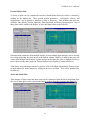
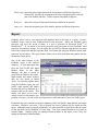
Ground Motion Plots
A variety of plots can be constructed from the Ground Motion Plots tab which is selected by
clicking on the labeled tab. Three ground motion parameters - acceleration, velocity, and
displacement - can be plotted as functions of time or frequency. Four different plot types are
available: Time History, Fourier Spectrum, Phase Spectrum, and Power Spectrum plots. Any of
these plots can be copied to the Report, or have their data written to the Data File.
Ground motion parameters from multiple depths, or from multiple input motions, can be selected
for a single plot using the check boxes in the Include column. While it is unlikely that users will
want to plot multiple time histories or phase spectra on the same plot, plots of multiple Fourier or
power spectra on the same graph can illustrate differences in frequency content effectively.
Time history of accelerations can also be saved to a file in PsoShake Input Motion Format for use
as input motion for future analysis by cliking on the Save As button. You will be prompted for
file name(s).
Stress and Strain Plots
Time histories of shear stress and shear strain can be constructed from the Stress and Strain Plots
tab. Any of these plots can be copied to the Report, or have their data written to the Data File.
27
ProShake User's Manual
Response Spectrum Plots
Response spectra can be plotted using the Response Spectrum Plots tab which is selected by
clicking on the labeled tab. Multiple response spectra, from different depths and/or for different
damping ratios or input motions, can be selected for a single plot using the check boxes in the
Include column.
Upon clicking the Plot button, acceleration spectra are plotted as a function of period on
arithmetic scales by default. However, velocity and displacement spectra can be plotted from the
plot form. Also, the abcissa can be changed to frequency and the scales to logarithmic from the
plot form.
All response spectrum plots can be copied to the Report, or have their data written to the Data
File.
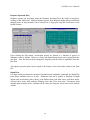
Depth Plots
It is often useful to examine the variation of ground motion amplitudes with depth; the Depth Plot
form allows ProShake users to do this. Parameters that can be plotted as functions of depth
include peak acceleration, peak velocity, peak displacement, peak shear stress, peak shear strain,
effective shear strain, shear modulus, damping ratio, and cyclic stress ratio. Parameters from
multiple input motions can be combined on the same plot using the check boxes in the Include
column.
28
ProShake User’s Manual
Parameters can also be copied to the report in tabular form by clicking Copy to Report button.
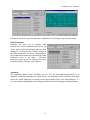
Other Parameters
ProShake will allow you to compute other
characteristics of the computed motion at the top
of any layer at which acceleration data has been
computed. Clicking on the Calculate button on
the Other Parameters tab allows computation of
the ground motion parameters shown on the Other
Parameters form to the right.
Calculated
parameter values can also be copied to the report
in tabular form by clicking Copy to Report.
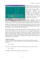
Animation
The Animation feature allows ProShake users to view the horizontal displacements of an
originally vertical line throughout an input motion. An animation can be viewed for each input
motion for which animation was selected on the Input Motion form in the Input Manager. To
view an animation, highlight the desired input motion and click on the Prepare Animation button.
29
ProShake User's Manual
ProShake will take a few moments to
load the data for the animation. The
animation is based on the computed
displacements at the top of each layer,
with
linear
interpolation
of
displacements
between
layer
boundaries. As a result, more realistic
animations can be achieved by
increasing the number of soil layers in
a profile; however, the increased
computational requirements will slow
program execution somewhat.
ProShake animations scale the
computed displacements so that the
maximum computed displacement is slightly less than the full-scale value of the horizontal axis.
This was done in order to clearly illustrate the pattern of the displacements; in most cases, the
amplitudes of the displacements will be greatly exaggerated. When used with input motions that
have not been baseline corrected, some apparent residual displacements may occur - these
displacements are relics of drift in the input motion and should not be taken to imply the existence
of residual strains (or stresses) in the equivalent linear analysis.
The ProShake animation can be played at three speeds - fast, real-time, and slow - and can be
started at any time during the record. Due to the speed limit of the Visual Basic graphics routine
that displays the animation, the fast and real-time speeds are accomplished by skipping different
numbers of time steps; hence, animations of some records may appear to “jump” a bit at those
speeds. Viewing the animation at the slow speed setting will provide a smoother view of the
displacement profile. For the example shown above, selecting a starting time of about 8 sec
would allow the most interesting part of the animation to be viewed in a reasonable amount of
time when the slow speed is selected.
Transfer Function Plots
A transfer function describes the relationship between two motions in the frequency domain.
Consider two motions, A and B, with Fourier Series A(f) and B(f), respectively. The motions can
be related by
A(f) = H(f) * B(f)
where H(f) is a transfer function. Therefore, the transfer function can be written as the ratio
H(f) = A(f)/B(f)
When damping is present, transfer functions are complex-valued.
30
ProShake User’s Manual
ProShake allows plotting of transfer functions between any two layers for any of the motions used
in the analysis from the Transfer Function form in Output Manager. A maximum of six different
transfer functions can be computed and plotted at one time using the check boxes in the Include
column. Transfer functions are computed using strain compatible modulus and damping values
obtained in the Solution Manager for the particular motion being used.
To plot the Transfer Functions, follow these steps:
1. Specify the Number of Frequencies (default = 201) and the Frequency Step (default = 0.1
Hz) for computing the transfer functions. Transfer function values will be computed and
plotted from 0 Hz to 20 Hz ( = [201-1]*0.1 Hz); the default values should provide
satisfactory resolution in most cases.
2. Click a check box in the "Include" column to specify a transfer function plot.
3. Click in the adjacent cell (in the Motion column). Use the drop down list box to select the
motion you want to use. The strain-compatible modulus and damping values for this
motion will be used to compute the transfer function.
4. Click in the next cell to the right (in the Layer A column). Select the Layer number you
want to use in the numerator of the transfer function equation.
5. In the column labeled Outcrop A, select whether to treat "Layer A" as an outcrop or
within profile motion.
6. Repeat Steps 4 and 5 for Layer B which will be in the denominator of the transfer function
equation.
Repeat Steps 2 through 6 to define additional transfer functions to be plotted. Any of the layers
can be defined as an outcrop or within profile for computing transfer functions. Then simply click
on the Plot button to create the transfer function plots.
Transfer functions, like all complex-valued functions, have real and imaginary part. The transfer
function can be expressed in terms of its real and imaginary parts as
H(f) = Re[H(f)] + i * Im[H(f)]
where Re[H(f)] and Im[H(f)] are the real and imaginary parts of H(f), respectively, and i2 = -1.
ProShake allows the transfer function to be plotted in four different ways:
Amplitude
shows the ratios of the amplitudes of the motions at different frequencies.
Numerically, given by the square root of the sum of the squares of the real and
imaginary parts of the transfer function.
31
ProShake User's Manual
Phase angle shows the phase angles between the two motions at different frequencies.
Numerically, given by the arctangent of the ratio of imaginary part to the real
part of the transfer function. Can be expressed in radians or degrees.
Real part
shows the real part of the transfer function at different frequencies.
Imag. part
shows the imaginary part of the transfer function at different frequencies.
Report
ProShake allows you to save numerical and graphical data in the form of a report - because
ProShake comes with its own Windows-based word processor. While the ProShake word
processor will serve the needs of many, it is not as powerful as Microsoft WordTM or
WordPerfectTM. If you prefer to use more powerful word processors, use the ProShake word
processor for temporary storage, save the report file in Rich Text Format using the Save As menu
item of the report form and later open the Rich Text Format file using the Windows-based word
processor of your choice. The report feature allows you to easily paste data and graphics into the
document of your choice.
One of the main features of the
ProShake report is the analysis
summary. As you enter input data
from the Soil Profile and Input
Motion forms in the Input
Manager, the data is stored in
arrays that are linked to the report.
Input motion and output location
data are also stored in linked
arrays. By selecting Update menu
from the ProShake report, the soil
profile, input motion, and output
location data will be displayed in a
compact table in the report. This
feature will allow you to keep a
written record of each analysis you
perform; of course, you can use the word processor to add comments of your own to the report.
By default, the report contains an Analysis Summary of the Soil Profile, Input Motion, and output
selections. Whenever you select "Copy to Report" the item of interest will be copied into the
report. Although items are copied sequentially, it is often advisable to type labels into the report
so that the items can be identified at a later time. Text items (usually numbers) are written in
column format. Graphics items are displayed black-on-white in the report, even if they are
displayed differently within ProShake.
32
ProShake User’s Manual
33
ProShake User's Manual
ProShake Graphics
ProShake allows rapid generation of many different types of plots. In the Input Manager, users
can plot modulus reduction and damping curves, various time histories and spectra for input
motions, and a graphical view of the soil profile. In the Output Manager, plots of time histories,
spectra, and depth variations are all available. Some of the common elements of these plots are
described in the following paragraphs.
For clarity on the computer monitor, the plots are displayed as light (generally yellow or white)
curves and axes on a darker background. The axes are selected to cover the entire range of data
and clearly illustrate the variation of the parameter being plotted. Nevertheless, some users may
want to change the characteristics of the plots - this is easily accomplished in ProShake.
To modify a plot, place the cursor anywhere on the plot and click the right mouse button. This
will produce a Graph Control dialog with tabs labeled Style, Data, Titles, Axis, Fonts, Markers,
Background, and System. These tabs allow virtually any characteristic of the plot to be modified
as the user desires.
The forms on which all ProShake plots are displayed also contain two buttons - one titled Copy to
Report and the other titled Write Data to File. The first copies the plot and pastes it into the
ProShake Report. The copy that goes to the report is formatted with black lines and axes on a
white background, even though the plot displayed on the screen is formatted differently. Users
may also want to save some data (e.g. ground motions or response spectra) for subsequent use or
additional processing. ProShake allows you to write data to an output file. The data is written
sequentially and labeled in the same manner as in the report.
Many of the ProShake plots have a Crosshair feature. This feature simply allows the user to see
the numerical values of the parameters that are being plotted. When the cursor is moved to the
plot area, it changes from an arrow to crosshairs and the values of the parameters at the locations
of the crosshairs are displayed.
34
ProShake User’s Manual
Theory
ProShake uses a frequency domain approach to solve the ground response problem. In simple
terms, the input motion is represented as the sum of a series of sine waves of different amplitudes,
frequencies, and phase angles. A relatively simple solution for the response of the soil profile to
sine waves of different frequencies (in the form of a transfer function) is used to obtain the
response of the soil deposit to each of the input sine waves. The overall response is obtained by
summing the individual responses to each of the input sine waves. This section describes the basic
mathematics of the process for a problem involving a single soil layer, illustrates how that problem
can be solved using a widely available mathematical programming language, and extends the
approach to layered systems.
Single Soil Layer
The following paragraphs describe the basis of the analysis used
in ProShake and follow the general approach of Kramer (1996).
That reference provides substantial background material and a
more detailed description of ground response analyses than is
presented in this User’s Manual.
zs
As
Bs
H
To illustrate the basic approach used in ProShake, consider a
Br
zr
Ar
uniform soil layer lying on an elastic layer of rock that extends to
infinite depth, as illustrated to the right. If the subscripts s and r
refer to soil and rock, respectively, the horizontal displacements due to vertically propagating
harmonic s-waves in each material can be written as
u s ( z s , t ) = A s e i (ω t + k s z s ) + B s e i (ω t − k s z s )
(1)
u r ( z r , t ) = A r e i (ω t + k r z r ) + B r e i (ω t − k r z r )
(2)
*
*
*
*
where ω is the circular frequency of the harmonic wave and k* is the complex wave number. No
shear stress can exist at the ground surface (zs=0), so
τ (0, t ) = G *s γ (0, t ) = G *s
∂ u s (0, t )
=0
∂z s
(3)
where G *s = G (1 + 2iξ ) is the complex shear modulus of the soil. Substituting Equation (1) into
Equation (3) and differentiating gives
(
)
G *s i k s A s e i k s (0) − B s e −i k s ( 0) e iωt = G *s i k s ( A s − B s) e iωt = 0
(4)
which is satisfied when As = Bs. Compatibility of displacements and continuity of stresses at the
soil/rock boundary require
35
ProShake User's Manual
u s ( z s = H ) = u r ( z r = 0)
(5)
τ s ( z s = H ) = τ r ( z r = 0)
(6)
Substituting Equations (1) and (2) into Equation (5)
(
)
*
*
As ei k s H + e −ik s H = Ar + B r
(7)
From Equation (6) and the definition of shear stress (τ = G *s ∂u ∂z )
(
)
(
)
*
*
As i G*s k *s ei k s H − e−i k s H = i G*r k *r ( Ar − Br )
or
G *s k *s
*
*
As ei k s H − e −i k s H = Ar − Br
*
*
Gr k r
(8)
The ratio
G *s k *s
= α *z
*
*
Gr k r
where α *z is known as the complex impedance ratio. Solving Equations (7) and (8)
simultaneously gives
[(
)
(
)
]
(9a)
[(
)
(
)
]
(9b)
Ar =
1
*
*
As 1 + α *z eik s H + 1 − α *z e−ik s H
2
Br =
1
*
*
As 1 − α *z ei k s H + 1 + α *z e −i k s H
2
If a vertically propagating shear wave of amplitude, A, traveled upward through the rock and the
soil was not present, the free surface effect at the rock outcrop would produce a bedrock
outcropping motion of amplitude 2A. If the soil was present, the free surface motion amplitude
would be
2 As =
(1 + α *z )
4A
*
eik s H
(
)
*
+ 1 − α *z e −i k s H
36
ProShake User’s Manual
The transfer function, F(ω), defined as the ratio of the soil surface amplitude to the rock outcrop
amplitude, is given by
F (ω ) =
(1 + α *z)
2
*
ei k s H
(
)
*
+ 1 − α *z e −i k s H
Obviously, the transfer function is a complex function. It can be rewritten using Euler's Law as
F (ω ) =
1
(10)
cos k *s H + i α *z sin k *s H
Solution of Single Layer Problem
Because the transfer function is defined as the ratio of the soil surface amplitude to the rock
outcrop amplitude, the soil surface amplitude can be obtained as the product of the rock outcrop
amplitude and the transfer function. Therefore, the response of the soil layer to a periodic input
motion can be obtained by the following steps:
1. Express the input (rock outcrop) motion in the frequency domain as a Fourier series
(as the sum of a series of sine waves of different amplitudes, frequencies, and phase
angles). For an earthquake motion, this Fourier series will have both real and
imaginary parts.
2. Define the transfer function (Equation 10). The transfer function will have both real
and imaginary parts.
3. Compute the Fourier series of the output (ground surface) motion as the product of
the Fourier series of the input (bedrock) motion and the transfer function. This
Fourier series will also have both real and imaginary parts.
4. Express the output motion in the time domain by means of an inverse Fourier
transform.
These steps are coded into a program using the mathematical processing program MATLAB in
the box located below. The syntax of a MATLAB program is similar to common languages such
as FORTRAN and BASIC, but MATLAB contains high-level functions that allow many
complicated calculations and graphics commands to be processed in a single line of text. The
MATLAB program is well-commented, and should be relatively easy to follow.
37
ProShake User's Manual
%
EX73.M - A MATLAB script for computing the seismic response of a uniform
%
damped soil layer on elastic bedrock. Input data corresponds to
%
Example 7.3 in Kramer, S.L. (1996), Geotechnical Earthquake
%
Engineering, Prentice Hall, 653 pp.
%
height=540;
% soil layer thickness
vss=1500;
% soil shear wave velocity
vsr=5000;
% rock shear wave velocity
rho_s=125;
% soil unit weight
rho_r=160;
% rock unit weight
xs=0.05;
% soil damping ratio
xr=0.02;
% rock damping ratio
load g1e.dat
% load input motion
n=length(g1e);
for j=2:n+1
a(j)=g1e(j-1)/981;
% shift and convert input motion to g’s
end
a(1)=0.0;
dt=0.02;
% time step
df=1./(n*dt);
% frequency increment
t=0.0:dt:n*dt;
% set up time vector
f=0.0:df:n*df;
% set up frequency vector
afft=fft(a)/n;
absfft=abs(afft);
for j=1:n/2+1
% set up single-sided FAS
b(j)=2.*absfft(j);
ff(j)=f(j);
end
alpha_z=(rho_s*vss*(1+i*xs))/(rho_r*vsr*(1+i*xr)); % complex impedance ratio
h(1)=1.0;
for j=2:n/2+1
ksH(j)=2*pi*f(j)*height/(vss+xs*i*vss);
% wave number x thickness
h(j)=1./(cos(ksH(j))+i*alpha_z*sin(ksH(j)));
% left half of transfer function
h(n+3-j)=conj(h(j));
% right half of transfer function
end
for j=1:n/2+1
habs(j)=abs(h(j));
% modulus of transfer function (for plotting)
end
subplot(5,1,1)
plot(t,a)
% plot input motion (time domain)
subplot(5,1,2)
plot(ff,b)
% plot FAS of input motion (frequency domain)
subplot(5,1,3)
plot(ff,habs)
% plot modulus of transfer function (freq. domain)
for j=1:n+1
acc(j)=afft(j)*h(j);
% compute output motion in frequency domain
end
for j=1:n/2+1
acc1(j)=2.*abs(acc(j));
% compute FAS of output motion
end
subplot(5,1,4)
plot(ff,acc1)
% plot FAS of output motion (frequency domain)
atime=n*real(ifft(acc));
subplot(5,1,5)
plot(t,atime)
% plot output motion (time domain)
The variables defined in the first part of the MATLAB program correspond to Example 7.3 in
Kramer (1996). This example considers the response of a 540 ft thick soil layer of soil (vss=1500
ft/sec, γ=125 pcf, and ξ=5%) overlying bedrock (vsr=5000 ft/sec, γ=160 pcf, and ξ=2%). The
MATLAB program generates the plots shown below.
38
ProShake User’s Manual
0.5
0
-0.5
0.020
5
10
15
20
25
30
35
40
0.01
0
0
4
5
10
15
20
25
5
10
15
20
25
5
10
15
20
25
2
0
0.020
0.01
0
0
1
0
-1
0
5
10
15
20
25
30
35
40
The first of these plots shows a time history of acceleration of the 40-sec input motion in the time
domain. Immediately below this is the Fourier amplitude spectrum of the input motion - the
Fourier amplitude spectrum shows the variation of amplitude with frequency for each of the
frequencies in the Fourier series. The abscissas of the second, third, and fourth plots are
frequency in Hz. The third plot shows the modulus (the square root of the sum of the squares of
the real and imaginary parts) of the transfer function. The transfer function is clearly seen to have
a series of local peaks that illustrate the nature of amplification that will take place at the natural
frequencies of the soil layer; note that the greatest amplification will take place at the lowest
natural frequency (where the transfer function reaches its global maximum). The fourth plot
shows the Fourier amplitude spectrum of the output (ground surface) motion which is numerically
equal to the product of the input motion (second plot) and the transfer function (third plot). The
origin of this spectrum is clearly seen by comparing the second, third, and fourth plots - the peaks
in the fourth plot (the output motion) are related to the peaks in the second plot (the input
motion) and the third plot (the transfer function). Finally, the last plot shows the output (ground
surface) motion in the time domain as obtained by taking the inverse Fourier transform of the
output motion in the frequency domain.
Multiple Soil Layers
The basic approach described in the preceding sections is also used to analyze layered soil
deposits in ProShake - the only difference is that the transfer function is different for a layered soil
deposit. The transfer function for a layered soil deposit must account for the transmission and
reflection of waves at boundaries between adjacent layers, much as those factors were accounted
for at the soil/rock boundary in the previous section.
39
ProShake User's Manual
Consider the soil deposit shown to the right. Within
a given layer, say layer j, the horizontal
displacements will be given by
( ) (
z1
h1
G1
x1
r1
z2
h2
G2
x2
r2
hϕ
Gϕ
xj
rj
h ϕ+1
G ϕ+1 xj+1 r j+1
hΝ
GN
zϕ
)
*
*
u j z j , t = A j ei k j z j + B j e −ik j z j eiωt
(11)
z ϕ+1
At the boundary between layer j and layer j+1,
compatibility of displacements requires that
zN
z N+1
A j +1 + B j +1 = A j eik j h j + B j e−i k j h j
*
*
xN
GN+1 x
r
N
r
N+1 N+1
(12)
Continuity of shear stresses requires that
A j +1 − B j +1 =
G*j k *j
G*j +1 k *j +1
* 
 A eik *sh j −
B j e−ik s h j 
 j
(13)
Note that Equations (12) and (13) are analogous to Equations (7) and (8), respectively. Defining
α *j as the complex impedance ratio at the boundary between layers j and j+1, the wave
amplitudes for layer j+1 can be obtained from the amplitudes of layer j by solving Equations (12)
and (13)
(
(
1
A 1 + α *j
2 j
1
B j +1 = A j 1 − α *j
2
A j +1 =
) ei k h + 21 B j (1 − α *j) e−i k h
) ei k h + 12 B j (1 + α *j ) e−i k h
*
j j
*
j j
(14a)
*
j j
*
j j
(14b)
At the ground surface ( z1 = 0 ), the requirement that the shear stress must be zero means that
A1 = B1 . Applying Equations (14) recursively for j = 1, 2, 3, …, N, the coefficients A j +1 and
B j +1 can be related to A j and B j by
A j +1 = a j +1 (ω ) A1
B j +1 = b j +1 (ω ) B1
(15a)
(15b)
where the functions a j +1 (ω ) and b j +1 (ω ) represent the effects of the wave interactions that
take place at all of the layer interfaces above layer j+1. Then, a transfer function relating the
motions at the tops of any two layers, say layers i and j, can be expressed as
40
ProShake User’s Manual
F ij (ω ) =
ai (ω ) + bi (ω )
a j (ω ) + b j (ω )
(16)
This transfer function can become quite complicated, but it is used in exactly the same way as the
much simpler transfer function developed for the single layer case. In fact, the MATLAB
program that illustrated the single layer case could be used to compute the response for a multilayered problem by changing only one line - the line where the transfer function is defined (with
the comment % left half of transfer function).
Equivalent Linear Analysis
The nonlinear and inelastic behavior of soil is well established in geotechnical engineering. The
nonlinearity of soil stress-strain behavior means that the shear modulus of the soil is constantly
changing. The inelasticity means that the soil unloads along a different path than its loading path,
thereby dissipating energy at the points of contact between particles. Rigorous analysis of the
mechanical response of soils to any type of loading, dynamic or otherwise, would require that the
stress-strain behavior of each element of soil be tracked directly in the time domain. The method
of analysis used in SHAKE (and ProShake) cannot allow for nonlinear stress-strain behavior
because its representation of the input motion by a Fourier series and use of transfer functions for
solution of the wave equation rely on the principle of superposition - which is only valid for linear
systems.
To approximate the actual nonlinear, inelastic response of soil,
τ
an equivalent linear approach can be utilized. In the equivalent
Gsec
linear approach, linear analyses are performed with soil
properties that are iteratively adjusted to be consistent with an
effective level of shear strain induced in the soil. In the
equivalent linear approach, the shear modulus is taken as the
γ
secant shear modulus which, as shown to the right,
approximates an “average” shear modulus over an entire cycle
of loading. As the level of shear strain increases, the secant
shear modulus decreases. The relationship between secant
shear modulus and shear strain amplitude can be characterized
by means of a modulus reduction curve. The nature of this
curve, which has an ordinate of modulus ratio (= G/Gmax) and an abscissa of log (shear strain), has
been well established for many soils. ProShake has a library of modulus reduction relationships
that can be selected in the Input Manager. The solution algorithm used in SHAKE (and
ProShake) assumes viscous soil damping which it represents using a complex shear modulus.
Viscous damping implies behavior that would be characterized by elliptical stress-strain loops.
Because actual stress-strain loops are seldom elliptical, an equivalent damping ratio is used - the
equivalent damping ratio is equal to the damping ratio that would be computed based on the area
within the hysteresis loop, the secant shear modulus, and the maximum shear strain. The
relationship between this equivalent damping ratio and shear strain is characterized by means of a
damping curve. The nature of this curve, which has an ordinate of damping ratio and an abscissa
of log (shear strain), has been well established for many soils. ProShake has a library of damping
41
ProShake User's Manual
curves that can be selected in the Input Manager.
In an equivalent linear analysis, the first iteration is performed using shear modulus and damping
ratios that correspond to some initially estimated level of shear strain. In ProShake, the first
iteration is based on an assumed shear strain of 0.001%. Following the first iteration, the effective
shear strain, defined as
γ eff = R γ γ max
where R γ is a strain reduction factor often taken as
Rγ =
M −1
10
is computed. The shear modulus and damping ratio corresponding to γeff is then used for the next
iteration. This process is repeated until the computed effective strain does not change much from
one iteration to the next. At this point, the equivalent linear process is said to have converged.
While the equivalent linear approach allows the most important effects of nonlinear, inelastic soil
behavior to be approximated, it must be emphasized that it remains a linear method of analysis.
The strain-compatible shear modulus and damping ratio remain constant throughout the duration
of an earthquake - when the strains induced in the soil are small and when they are large.
Permanent strains cannot be computed and porewater pressures cannot be computed. However,
the equivalent linear approach has been shown to provide reasonable estimates of soil response
under many conditions of practical importance.
42
ProShake User’s Manual
Verification
As stated earlier in the User’s Manual, ProShake was written from scratch using the same
computational procedure used in the original version of SHAKE (Schnabel et al., 1972). Though
the basic procedures are the same, some aspects of their numerical implementation were different.
As a result, verification of the accuracy of ProShake and comparison of its results with the results
from previous versions of SHAKE are required.
Verification Using Analytical Solutions
ProShake has been verified against exact analytical solutions for the simple loading cases for
which such solutions are available and found to produce accelerations that match the exact
solutions perfectly to at least the first six decimal points (with acceleration measured in g’s).
Comparison with SHAKE
Additional verification of the numerical implementation of ProShake can be obtained by
comparing its results with those of previous versions of SHAKE when both are applied to the
same problem. Because SHAKE91 is the most commonly used version of SHAKE in current
geotechnical earthquake engineering practice, a number of such comparisons between ProShake
and SHAKE91 have been performed; the results of a typical comparison are described in this
section.
The numerical implementation of ProShake differs from that of SHAKE91 in the following ways:
1. ProShake uses 32-bit arithmetic rather than the 16-bit arithmetic used in
SHAKE91. This is primarily a result of recent advances in development platforms 32-bit Fortran became available for personal computers after the development of
SHAKE91 and before the development of ProShake.
2. ProShake uses a different Fast Fourier Transform (FFT) routine. The routine used
in ProShake, taken from the International Mathematical Software Library (IMSL),
represents a more recent and efficient implementation of the FFT.
3. ProShake uses a more efficient and robust procedure to iterate toward straincompatible soil properties. For most analyses, the last iteration required to drop the
modulus and damping error below the specified error tolerance in ProShake will
produce smaller final errors than the last iteration for the same error tolerance in
SHAKE91.
4. ProShake handles cutoff frequencies slightly differently than SHAKE91.
SHAKE91 applies its cutoff frequency after scaling the input motion to the
specified peak acceleration; as a result, the actual peak acceleration used in the
analysis can be different than the desired peak acceleration. ProShake applies the
cutoff frequency before any required scaling - in this way, the accelerations that are
actually used as input in the analysis are equal to the desired accelerations. The
43
ProShake User's Manual
difference between these approaches is small for reasonably high cutoff frequencies,
but the approach taken in ProShake is considered to be more appropriate.
The relative performance of ProShake and SHAKE91 can be illustrated using the example
problem from the original SHAKE User’s Manual (Schnabel et al., 1972). This problem, for
which the input file is contained in the file shake.dat, involves the response of a 150-ft-thick soil
deposit. Analyzing the deposit using both ProShake and SHAKE91 produces the time histories of
ground surface acceleration shown below:
0.25
SHAKE91
0.20
ProShake
Acceleration (g)
0.15
0.10
0.05
0.00
-0.05 0
5
10
15
20
25
Time (sec)
-0.10
-0.15
-0.20
-0.25
The differences between the ground surface accelerations produced by ProShake and SHAKE91
are very small. To make these differences more apparent, portions of the time histories are
expanded in the two plots shown below:
0.25
SHAKE91
0.20
ProShake
Acceleration (g)
0.15
0.10
0.05
0.00
-0.05 10
11
12
13
14
15
Time (sec)
-0.10
-0.15
-0.20
-0.25
44
ProShake User’s Manual
0.25
SHAKE91
0.20
ProShake
Acceleration (g)
0.15
0.10
0.05
0.00
-0.0511.0
11.2
11.4
11.6
11.8
12.0
Time (sec)
-0.10
-0.15
-0.20
-0.25
Even when the time scale is expanded tremendously, the strongest part of the computed
response shows very close agreement between the two programs.
Shear Modulus (ksf)
Spectral Acceleration (g)
The programs can also be compared from the
1.0
standpoint of response spectra - the
SHAKE91 (5%)
0.9
computed ground surface response spectra
SHAKE91 (10%)
0.8
ProShake (5%)
for structural damping ratios of 5% and 10%
ProShake (10%)
0.7
are illustrated to the right. Again, the
0.6
response spectra are very similar (in fact, part
0.5
0.4
of the differences in these plots is explained
0.3
by the fact that ProShake and SHAKE91
0.2
compute spectral accelerations at different
0.1
periods. Another comparison can be made
0.0
0.0
0.5
1.0
1.5
2.0
2.5
with respect to the equivalent linear
Period (sec)
properties that both programs converge to.
The equivalent linear shear moduli from the final iteration of ProShake and SHAKE91 are shown
below. Again, the very close agreement between the moduli from the two programs verifies their
consistency.
15000
10000
5000
SHAKE91
ProShake
0
0
50
Depth (ft)
100
150
The same set of comparisons can be made for other ground response problems. The following
plots compare the responses predicted by ProShake and SHAKE91 when both are applied to the
45
ProShake User's Manual
problem described in the Tutorial section of this User’s Manual. The tutorial problem involved a
50 ft thick layer of soft silty clay overlaying a 50 ft thick layer of stiff clay. The thick, soft nature
of the silty clay layer also produces ground surface motions with relatively low accelerations and
long periods. The following plot illustrates this response:
Acceleration (g)
0.15
SHAKE91
0.10
ProShake
0.05
0.00
-0.05
0
5
10
15
20
25
30
Time (sec)
-0.10
-0.15
Again, the differences between the ground surface accelerations produced by ProShake and
SHAKE91 are very small, even when the time scale is expanded as shown below:
Acceleration (g)
0.15
SHAKE91
0.10
ProShake
0.05
0.00
-0.05
10
11
12
13
14
15
Time (sec)
-0.10
-0.15
Acceleration (g)
0.15
SHAKE91
0.10
ProShake
0.05
0.00
11.0
-0.05
11.2
11.4
11.6
11.8
12.0
Time (sec)
-0.10
-0.15
46
ProShake User’s Manual
Shear Modulus (ksf)
0.5
Spectral Acceleration (g)
Response spectra are also very similar
as illustrated (for structural damping
ratios of 5% and 20%) to the right. The
distinguishing feature of the tutorial
problem, from the ground response
standpoint, is the presence of the strong
impedance contrast at the boundary
between the soft silty clay and the stiff
clay. This impedance contrast causes
large strains near the bottom of the soft
silty clay layer that lead to low shear
moduli in the equivalent linear model.
SHAKE91 (5%)
SHAKE91 (20%)
ProShake (5%)
ProShake (20%)
0.4
0.3
0.2
0.1
0.0
0.0
0.5
1.0
1.5
Period (sec)
2.0
2.5
1500
1000
SHAKE91
500
ProShake
0
0
10
20
30
40
50
Depth (ft)
47
60
70
80
90
100
ProShake User's Manual
Strong Motion Parameters
Arias Intensity
The Arias Intensity (Arias, 1970), also influenced by amplitude, frequency content, and duration,
is defined as
Ia =
π ∞
∫ [a(t )]2dt
2g 0
The Arias Intensity has units of velocity and is usually expressed in meters per second. Since it is
obtained by integration over the entire duration, rather than over the duration of strong motion,
its value is independent of the method used to define the duration of strong motion.
Bracketed Duration
The bracketed duration is the time interval between the first and last exceedances of a threshold
acceleration (Bolt, 1969). The threshold acceleration is set at 0.05g in ProShake.
Peak Acceleration
The maximum absolute value of acceleration. The peak acceleration provides a useful measure of
the strength of the higher frequency components of a ground motion.
Peak Velocity
The maximum absolute value of velocity. The peak velocity provides a useful measure of the
strength of the intermediate frequency components of a ground motion.
Peak Displacement
The maximum absolute value of displacement. The peak displacement provides a useful measure
of the strength of the lower frequency components of a ground motion.
Predominant Period
The predominant period is the period corresponding to the maximum value of the Fourier
spectrum. Because Fourier spectra are typically quite jagged, the period corresponding to the
highest peak in a raw spectrum may not correspond well to the strongest part of the motion. For
that reason, some users may want to obtain predominant periods from smoothed spectra. The
cross-hair feature can be used to estimate predominant period from ProShake Fourier spectrum
plots.
Response Spectrum Intensity
The response spectrum intensity (Housner, 1959) is defined as
2.5
SI (ξ ) = ∫ PSV (ξ , T )dT
0.1
48
ProShake User’s Manual
i.e., the area under the pseudo-velocity response spectrum between periods of 0.1 second and 2.5
seconds. In ProShake, the response spectrum intensity is computed for a structural damping ratio
of 5%. It captures important aspects of the amplitude and frequency content (in the range of
primary importance for structures) in a single parameter.
RMS Acceleration
The RMS acceleration is a single parameter that includes the effects of the amplitude and
frequency content of a strong motion record
a RMS =
1
Td
Td
0
2
∫ [a(t )] dt
where Td is the duration of the motion. Because the integral is not strongly influenced by large,
high frequency accelerations (which occur only over a very short period of time) and because it is
influenced by the duration of the motion, the rms acceleration can be very useful for engineering
purposes. ProShake uses the Trifunac duration for computation of the RMS acceleration.
Trifunac Duration
The Trifunac duration (Trifunac and Brady, 1975) is defined as the time interval between the
points at which 5% and 95% of the energy in a ground motion have been delivered. Numerically,
it corresponds to the time between the 5% and 95% points on a Husid plot.
49
ProShake User's Manual
Built-In Soil Models
Vucetic-Dobry
Vucetic and Dobry (1991), building on the work of Kokoshu (1980) in an investigation motivated
by the performance of Mexico City clay in the 1985 Michoacan earthquake, showed clearly how
modulus and damping behavior are influenced by soil plasticity. Vucetic and Dobry developed
families of modulus reduction and damping curves as functions of plasticity index. ProShake
allows you to specify any plasticity index - the program will determine the corresponding curves
by interpolation. The curves originally proposed by Vucetic and Dobry are shown on the plots in
green; from left to right, they represent PI = 0, PI = 15, PI = 30, PI = 50, PI = 100, and PI = 200.
The curve for the selected PI is obtained by linear interpolation and shown in yellow. See also
Dobry and Vucetic (1987).
Sun, Golesorkhi, and Seed
Sun, Golesorkhi, and Seed (1988) developed a series of modulus reduction and damping curves
for different ranges of plasticity index. Separate curves for 5 < PI <10, 10 < PI < 20, 20 < PI <
40, 40 < PI < 80, and PI > 80 were developed. ProShake will ask for the plasticity index of the
soil, and use it to assign the proper curve (i.e., it does not interpolate).
Ishibashi-Zhang
Modulus reduction and damping characteristics, particularly for low-plasticity soils, are also
influenced by effective confining pressure. Ishibashi and Zhang (1993) proposed expressions for
shear modulus and damping ratio that accounted for plasticity index and effective confining
pressure. ProShake will compute the effective confining pressure, but you must provide the
plasticity index. In calculating the effective confining pressure an at rest earth pressure coefficient
(K0) of 0.5 is assumed. It should be noted that the actual Ishibashi and Zhang equations predict
G/Gmax values slightly greater than 1 over a range of low strains. ProShake sets G/Gmax = 1.0 for
these values. . ProShake does not modify the damping curves, however, for the effects of this
limiting value. See also Ishibashi (1992).
Seed-Idriss Sand
Seed and Idriss (1970) developed the first widely used modulus reduction and damping curves for
sand. Their curves showed a range of modulus reduction behavior. ProShake allows you to
select the average of that range, or the upper or lower bounds.
Gravel
Seed at al. (1984) developed modulus reduction and damping curves for gravel. These curves are
based on the average behavior of 12-inch diameter cyclic triaxial tests on four different gravels.
Rock
Modulus reduction and damping curves for rock were included in sample data files for the original
SHAKE program (Schnabel et al., 1970).
50
ProShake User’s Manual
Linear
ProShake allows you to specify a linear elastic or linear viscoelastic material. When you select
this material, ProShake will use the maximum shear modulus and prompt you to enter a damping
ratio. You should note that the transfer function for an undamped linear elastic layer will have
singularities at the natural frequencies of the layers; these can lead to numerical problems that
prevent program execution.
51
ProShake User's Manual
Definitions
Analysis Summary - a summary of the soil profile, input motion, and output selections for the
analysis. The analysis summary is written to the Report - from there, it can be printed and placed
in a project or assignment file.
Cyclic Stress Ratio - the ratio of the peak shear stress to the vertical effective stress.
Damping Error - the difference between damping ratio values in successive iterations divided by
the damping ratio value used in the most recent iteration (expressed as a percentage).
Drag-and-Drop - By holding the left mouse button down, any line (corresponding to a particular
material layer) can be copied and placed at the location of the cursor at the time the left mouse
button is released.
Effective Shear Strain - The amplitude of a harmonic (sinusoidal) shear strain time history that
would be equivalent to the time history of shear strain from an actual earthquake record. The
effective shear strain is equal to the product of the maximum shear strain and the strain ratio.
Frequency Content - the distribution of acceleration amplitudes in the frequency domain. The
frequency content can be obtained from the shape of the Fourier spectrum of the motion.
Impedance Ratio - the ratio of specific impedances of two adjacent soil layers, where the specific
impedance is defined as the product of the density and shear wave velocity of a material.
Input Motion Format - ProShake input motion files are formatted in a certain way. The two
input motion files included in the distribution of ProShake, yerba.eq and treas.eq, are in the proper
format. Input motion files in any other format can be converted to ProShake Input Motion
Format by using the Convert Ground Motion File utility.
Modulus Error - the difference between shear modulus values in successive iterations divided by
the shear modulus value used in the most recent iteration (expressed as a percentage).
Peak Acceleration - the maximum (absolute) value of acceleration in an acceleration time history.
Peak Displacement - the maximum (absolute) value of displacement in a displacement time
history.
Peak Shear Strain - the maximum (absolute) value of shear strain in a shear strain time history.
Peak Shear Stress - the maximum (absolute) value of shear stress in a shear stress time history.
Peak Velocity - the maximum (absolute) value of velocity in a velocity time history.
52
ProShake User’s Manual
Quiet Zone - a portion of an input motion with zero (or very small) accelerations. Because the
frequency domain solution of ProShake implies periodicity (i.e., that the input motion repeats
itself indefinitely), a quiet zone may be required for the computed response to an individual
application of the input motion to be distinct.
Tab Label - the label found on the protruding portion of a tab form. The tab label shows which
of the tab forms is active. Only one tab form can be active at a time.
Trailing Zeroes - acceleration values of 0.0 that are appended to the end of an input motion file
to bring the total number of acceleration values to an integer power of 2.
53
ProShake User's Manual
References
Dobry, R. and Vucetic, M. (1987). "Dynamic properties and seismic response of soft clay
deposits," Proceedings, International Symposium on Geotechnical Engineering of Soft Soils,
Mexico City, Vol. 2, pp. 51-87.
Housner, G.W. (1959). “Behavior of structures during earthquakes,” Journal of the Engineering
Mechanics Division, ASCE, Vol. 85, No. EM14, pp. 109-129.
Idriss, I.M. and Sun, J.I. (1992). “SHAKE91: A computer program for conducting equivalent
linear seismic response analyses of horizontally layered soil deposits,” User’s Guide,
University of California, Davis, California, 13 pp.
Ishibashi, I. (1992). Discussion to "Effect of soil plasticity on cyclic response," by M. Vucetic and
R. Dobry, Journal of Geotechnical Engineering, ASCE, Vol. 118, No. 5, pp. 830-832.
Ishibashi, I. and Zhang, X. (1993). "Unified dynamic shear moduli and damping ratios of sand and
clay," Soils and Foundations, Vol. 33, No. 1, pp. 182-191.
Kokoshu, T. (1980). "Cyclic triaxial test of dynamic soil properties for wide strain range," Soils
and Foundations, Vol. 20, No. 2, pp. 45-60.
Kramer, S.L. (1996). Geotechnical Earthquake Engineering, Prentice Hall, Upper Saddle River,
New Jersey, 653 pp.
Schnabel, P.B., Lysmer, J., and Seed, H.B. (1972). "SHAKE: A computer program for
earthquake response analysis of horizontally layered sites," Report No. EERC 72-12,
Earthquake Engineering Research Center, University of California, Berkeley, California.
Seed, H.B. and Idriss, I.M. (1970). "Soil moduli and damping factors for dynamic response
analyses," Report No. EERC 70-10, Earthquake Engineering Research Center, University of
California, Berkeley.
Seed, H.B., Wong, R.T., Idriss, I.M., and Tokimatsu, K. (1986). Moduli and damping factors for
dynamic analyses of cohesionless soils," Journal of Geotechnical Engineering, ASCE, Vol.
112, No. 11, pp. 1016-1032.
Sun, J.I., Golesorkhi, R., and Seed, H.B. (1988). "Dynamic moduli and damping ratios for
cohesive soils," Report No. EERC-88/15, Earthquake Engineering Research Center,
University of California, Berkeley.
Vucetic, M. and Dobry, R. (1991). "Effect of soil plasticity on cyclic response," Journal of
Geotechnical Engineering, ASCE, Vol. 117, No. 1, pp. 89-107.
54