1
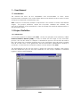
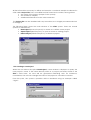
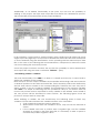
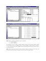
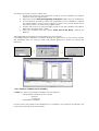
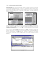
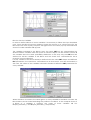
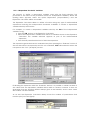
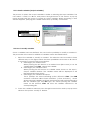
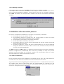
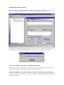
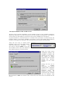
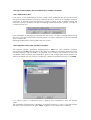
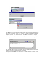
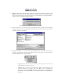
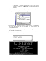
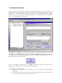
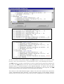
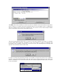
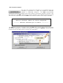
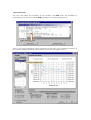
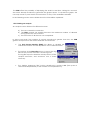
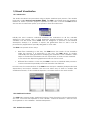
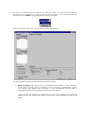
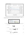
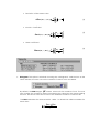
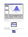
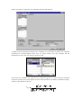
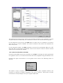
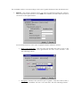
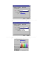
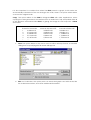
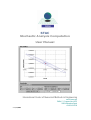
STAC Stochastic Analysis Computation User Manual International Center of Numerical Methods in Engineering www.cimne.com Edifici C1, Campus Nord UPC 08034 Barcelona Spain +34 93 4016036 v. 11/3/2005 1. - User Manual 1.1 Introduction This manual will show all the capabilities and functionalities of STAC. Some representative examples of the code will be discussed in detail in order to point out and avoid errors frequently committed by users. STAC stands for "Stochastic Analysis Computation" and consists of three well defined stages: The project definition, where the stochastic variables are defined, the execution definition of the deterministic code and finally the statistical representation of the generated data. 1.3 Project Definition 1.3.1 Introduction A stochastic problem is defined with STAC via the GUI (Graphic User Interface) called Problem Definition Module (PDM). In order to define the first stage of any stochastic process, the user first needs to analyze a deterministic process and obtain all solution files. This means the complete problem has to be executed using all solvers involved and all I/O files have to be generated. All this information (deterministic analysis) is necessary, so that later the stochastic analysis can be defined with STAC. The deterministic I/O files are the basis to define the stochastic variables, their format and the distribution type for the input variables. For the output variables a statistical register is defined and initialized. MDP All the information necessary to define and execute a stochastic analysis is collected in a file called Project File. This is a small file in ASCII format that contains, among others: • the name of the Project (unique for the system) • the number of samples • additional information for the solver execution The Project File can be visualized with any text editor, but it is highly recommended not to change it. The following figure shows the main window of the STAC system. There are several options to choose from: • New Project (Nuevo Proyecto) to create or to define a new project • Open Project (Abrir Proyecto) to open a recent or existing project. • Delete Project (Eliminar Proyecto) to delete a project 1.3.2 Creating a new Project When the user selects the option New Project, a new window is displayed to query the new project’s name. If the name already exists as a project previously stored in the STAC’s data base, an error will be generated indicating such an incidence; nevertheless, the user can change the name of his project or cancel the creation. From this point, the system’s operation will be described using an example called “Viga1”. Additionally, as an added functionality at this point, the user has the possibility of adding to the project the input and output files that define the deterministic process. This functionality is presented later in the project definition. In this example, a new project is created (Viga1) with a single input file (Viga.cal) and a single output file (Viga.sal). It is important to remark that the results files must correspond to those obtained using the deterministic solver operating with the selected input data files. In the case of not following this recommendation, unexpected or erroneous results can occur during the stochastic process. Once the project has been created, the user has the possibility to add or delete input and output files using the menu command “Ficheros” (Files). 1.3.3 Defining random variables The main functionality of the PDM is to allow, in a simple and fast way, to select and to define the variables of the problem. Both the input and the output variables are treated like ASCII strings and are located in a absolute positions in the data and results files. These absolute positions are defined by the line and column number in the corresponding file. Therefore the user only has to select a value to use as a random variable. The specification of the random variables with STAC is as simple as selecting the text (numerical value) of our interest with the mouse. This process must be repeated for every variable to be defined. More details of this one process will be described in later sections. The following figures show this process in an input and an output file. When defining a variable, the user should keep the following points in mind. Any violation of these rules will cause the variable creation to be canceled. • Only numerical characters must be selected. • When there is more than one variable in a row, only one can be selected at a time. • If the variable can have a positive and a negative sign, and the variable appears as positive in the input data file, it is necessary to add a space to consider the possible negative values. STAC allows to define two different types of variables: • Scalar Variables • Vector Variables An example of how to select a scalar variable is shown in the previous figures, where the user selects only one variable at time. A vector variable, or better known as a Block, is a set of at least two scalar variables of the same length located in the same position in consecutive lines. STAC offers a simple mechanism to select a Block. A Block is defined by two points: the upper left corner and the lower right corner as shown in the figure below The steps necessary to select a Block are: 1. Position the mouse on the upper left corner of the first variable of the Block and then press the right button. 2. Select the option mark the beginning of the Block. (Marcar Inicio de Bloque) 3. A new window appears to select the periodicity of the variables in a Block. This functionality is useful, since it allows to select only certain fields with a repetitive pattern, as shown in the figure below 4. Position the mouse on the lower right corner of the last variable of the Block and press the right button again. 5. Finish the selection with the option mark end of the Block. (Marcar Fin Bloque) The beginning and end block marks must be in the same file. Canceling a Block definition is possible clicking the right button of the mouse outside the selecting area. An pop-up menu will appear giving the option to cancel the selection. 1.3.3.1 Random variables (Input variables) In STAC two types of stochastic variables can be defined: − Independent variables, these can be: − Discreet − Continuous − Dependent variables. In both cases, the selection and definition of a variable is very intuitive and simple. The next section describes this mechanism. 1.3.3.1.1 Independent Stochastic Variables. Scalar Variables In order to make the selection of a scalar random variable, is necessary to find the corresponding variable field in the proper input file, and with the left mouse button pressed select the length of the field. Clicking the right mouse button on the selected field will cause a floating menu to appear, showing all the probability distributions functions available. Once the probability distribution function has been selected (PDF), a new window appears describing the PDF chosen its shape and suggested parameters. The user can change the parameters function to fit the PDF at his/her requirements. A brief example is shown in the next figures. In the case of a Normal PDF (Gaussian function), STAC automatically assigns the selected value to the average (µ) and a value of 0,1µ to the standard deviation (σ). Also the interval where the PDF shape will be shown is defined by the interval (µ−3σ , µ+3σ ). These values can be modified by the user and are described in detail in ANNEX A. Block or Vector Variables In order to define a Block or Vector variable, it is necessary to follow the steps described next. Once the Block has been marked, locate the mouse on a colored zone (in the Block case the zone is pink) and press the right button. The same pop-up menu like that shown for scalar variables will appear. The variables included in the Blocks have the same PDF but are characterized by distinct random variables. With this option a uniform sample can be created, where all the variables have the same probability distribution. In this way only one PDF must be defined for all the variables in the Block and the check box “Uniformizacion de la muestra” must be selected. If every variable in the block should be defined with the same PDF shape and different PDF parameters, the check box “Uniformizacion de la muestra” must be unchecked. In this case, the values of the variables selected in the Block define the PDF parameters for every variable. When the Block is created, the name given to every variable in the Block contains the Block Name and an index indicating the position in the Block. In the example shown, if a Block of 2 variables is created, the name of these variables will be: Bloque_Normales_1 and Bloque_Normales_2, respectively. 1.3.3.1.2 Dependent Stochastic Variables The process to define a dependent variable starts with the field selection. This procedure is the same as the procedure shown for independent variables. When the floating menu appears, select the option Dependent (“Dependiente”) and the Expression Calculator will be accessible The Expression Calculator allows to define a function using any type of mathematical expressions involving the Independent Stochastic Variables to create a dependent variable ruled by this function. For example, to create a dependent variable ruled by the SIN of the independent variable Young, Press the SIN button in the Expression Calculator Select an independent variable from the list of variables shown in the Expression Calculator. The variable selected appears as part of the mathematical expression. Press the left parenthesis button to finish the expression. The expression generated can be evaluated any time pressing the “Evaluate” button. If the user introduces an expression and it is not evaluated, STAC will evaluate it when the user presses the “OK” (“Aceptar”) button. Evaluating the expression with the “Evaluate” button, it is possible to obtain an idea of the values that the dependent variable will be able to assume, however it does not guarantee that the function defined always gives a real number, and in some cases the number can be indefinite. As an aid, the Expression Calculator always shows the number of parentheses that remain open (see next figure). 1.3.3.2 Results variables (Output variables) The process to select the output variables is similar to selecting the input variables. The user selects a field, or a Block, and presses the right button of the mouse. A pop-up menu appears with the option to create an output variable. When accepting, a new window appears, querying the variable name and, optionally, a comment. 1.3.4 How to modify variables Once a variable has been defined, the user has the possibility to modify or unselect it. The procedure is the same for all kinds of variables and is described below: 1. Select the variable to modify or unselect. The selection can be made in three different ways. In the figure below the three possibilities are shown. In all cases it is necessary to press the left mouse button. a. Selecting by the marked zone. When pressing the left button on a marked zone (blue zone) or on the variable field itself, STAC selects the variable. b. Selecting by the variable name. When pressing the left button on variable name shown on the Input / Output variable window. The variable name will be displayed in the hierarchical structure shown. c. Selecting by the variable descriptor. This is perhaps the more interesting option offered in STAC. The PDM contains a window called “Data Overview” (“Vista de Datos”), where all the selected variables are listed and presented with useful information like the variable type, size, PDF type, etc. When pressing the variable name on this window, STAC will show the variable selected in the corresponding file. 2. Once the variable is selected, press the right mouse button and a pop-up menu will show the options: Modify or Delete. 1.3.4.1 Modifying a Variable If the Modify option was selected, STAC will present the adequate window depending on the variable type (the PDF window, the Expression Calculator, or the Output Variable window). Then, all the parameters can be reentered and changed except for the variable name that can not be modified in any way. If an independent variable is modified and it is associated with some dependent variables, STAC will recalculate all these dependent variables informing if the procedure was successful or not. If some type of error occurred during the dependent variable actualization (division by zero, etc) the changes defined in the dependent variable will not take effect. 1.3.4.2 Deleting a Variable If the Delete option was selected STAC will eliminate the variable selected. If an independent variable is eliminated, it can happen that this variable forms part of one or several dependent variables. Should this be the case, a message indicates it and STAC will delete the independent variable and all the associated dependent variables. 1.4 Definition of the execution process In order to complete the definition of a project, it is necessary to declare: The sample size or the number of runs. The maximum number of wrong runs. This is the number of times that solver execution ends without producing output variables. The necessary commands for the solver execution. The additional files needed by the solver. The Working Directory, where all the generated files will be saved temporarily during the analysis process. The Service Directory, where the data corresponding to the results obtained during the different executions will be saved. Later, this data will be processed to show the results graphically. The GUI provided by STAC allows to define and execute all the processes needed to perform a single shoot. Additionally STAC offers the possibility to verify the process definition before launching the stochastic analysis. This functionality allows to reduce the time needed to define the execution process. 1.4.1 Initial considerations In this document the process definition is presented step by step. The order followed is not relevant so the user can complete the steps presented in any order. A good practice before beginning the execution process- is to declare the location of the Working and Service Directories. Both are indispensable for carrying out the stochastic execution. The user can define and redefine these directories at any time, except for during the process execution. ADM (Analysis Definition Module) When the option execute (ctrl+E) is selected, the window shown below appears. This window contains all the tools needed to define the execution of a process. Is necessary to fulfill all the requirements in this window, if not, trying to run a process will result in an error message indicating the missing steps, as shown in the next figure. Error message: It is necessary to set the number of runs. 1.4.2 Step 1: Definition of the Service and Working directories. Selecting the Options (“Opciones..:”) choice on the Execute (“Ejecutar”) menu of the top bar, The Service and Working Directory window will appear. In the folder marked “Directorios” there is a button for each directory which allows to change or redefine- a new path. When a new project is created, the default directories are shown. However, the user can specify any directory, including those located in a local area network. 1.4.3 Step 2: Definition of the number of runs. The size of the process population or the number of runs in the stochastic analysis is defined in this phase. It is also necessary to set the number of wrong runs. A wrong run occurs when it is impossible to read any of the output variables for any reason. A good practice Is recommended to consider some processes to fail because the random nature of the input variables can cause a run to fail. When the maximum number of wrong runs is reached, the stochastic process will stop automatically. There are two ways to define these numbers. One is via the main menu – “Ejecutar->Opciones, "General" - and the other is using the ADM. In this case, the number of runs must be entered in the sample size box as shown beside. Using the main menu command, besides the possibility to define the number of runs, there is the option to delete temporary files created during the previous analysis for the same project During the first run of every analysis execution, the button “Delete Files” (“Eliminar Archivos”) is disabled, however once the analysis has ended, the temporary files created can be deleted. Only files created by STAC are deleted, files created by the solvers are not included in this option. 1.4.4 Step 3:Add auxiliary files and Define Input variable correlation. 1.4.4.1 Add auxiliary files If the solver, or the deterministic process, needs some additional files (not produced by the process itself) different from those defined the Input and Output variable section is necessary to provide them beforehand in order for them to be available during the sochastic process. Examples are files containing material properties, groups of nodes or a data structure etc. If an existing file in the project is added with this option, an error message will inform of this fact. It is evident that a file containing input or output variables can not be defined as an auxiliary file. Deleting auxiliary files is also possible with this option. 1.4.4.2 Definition of the Input variable correlation. The random number generator implemented in STAC not only produces numbers according to the PDF selected, but is also able to establish a correlation between these random numbers. This capability is a powerful tool to reduce the number of runs. The correlation value between two variables is given in the spread sheet shown below. This table is obtained with the “Definir Correlacion” (Define Correlation) button of the ADM If no value is given, a correlation zero is applied. Zero correlation is also the default value. The correlation between two variables is a number between -1 and 1. If the introduced absolute value is greater than 0,85 , STAC suggests to use dependent variables. 1.4.5 Step 4: Batch command definition The ADM includes many tools to assist in the creation and testing of the batch file to run the process. A batch file consists of a sequence of MS-DOS commands to define the working directories, the solver commands, and all the instructions to complete a deterministic analysis. STAC will launch this batch file as many times as the sample size defined by the user- to perform a- stochastic analysis. The ADM provides a specific window in which the batch commands can be specified. The batch file will be saved in the Working directory. This file will be recovered if the project is opened to avoid reentering the commands. There is a tool bar available (see figure below) to simplify writing the batch file. A brief description of the functionality of each button will be given next. 1. Import a batch file. As the name indicates, this button allows to include in the ADM a batch file previously written (the file extension must be bat). Two options exist: The imported file is a new sequence of commands or the imported file is added to the commands already written. Would you like to add the file to the current data? 2. Save a batch file. This option saves the batch file under another name, allowing the user to recover it later. With this option the written batch file can be used for another project or program.- 3. File Name Helper. This is one of the most useful buttons. This drop-down button consists of the options shown in the figure below, and inserts the selected path and the file name into the batch file. “Agregar Work Dir” inserts the Working directory path. If it has not been defined, nothing is inserted. “Agregar Dir…” Inserts the name and path of any directory. The directory selection is made using the GUI for file management provided by Windows. STAC inserts the short name of a directory to guarantee the compatibility between Win95/98/Me and Nt/2000/Xp platforms. “Agregar File …” Insert the name and path of any file. The directory selection is made using the GUI for file management provided by Windows. It is possible to add the names (and path) of the input and output variable files to the batch file with a simple click of the mouse - left button - on the file name that appears in the file explorer as shown in the figure below. 4. Test the Batch File. This option is offered to test the sequence of commands in the batch file. This utility can serve to validate and correct errors in the deterministic execution. 5. Help. This button gives access to a small guide and some suggestions useful for the batch file commands edition. The figures below show the batch file for running the example and the DOS window shown when the “Test Batch File” button was pressed. 1.5 Analysis Execution When the process definition is complete, the stochastic analysis can be performed. In the example shown in the figure below, all the process data is specified. Now, to run an analysis, it is only necessary to press the button “Comenzar Ejecución” (Begin Execution), or, in the menu bar, submenu “Execute”, the option “Ejecutar” (Execute). Any of the options presented is valid. The PDM and the ADM are the modulus in charge of the problem definition. Once the execution of the analysis begins, the Execution Module (EXM) is activated. This module is in charge of the analysis management from the random variable generation to the gathering of the output variables. When the stochastic analysis starts, the EXM activates a window that shows all the details of the execution state, as shown in the next figures. The information shown includes: State of the temporary files necessary to boot the execution. (“inicializando variables”) State of the evolution of the stochastic analysis for each run and statistics about the number of completed and erroneous runs. As can be seen in the previous figure, the EXM window contains two buttons: “PostProcess” and “Cancel Execution” (“Cancelar Ejecución”). The meanings are obvious. The EXM window contains a check box to show or hide the DOS execution window for the solver. The EXM detects that the solver has finished the execution when the DOS window closes. In systems based on the MSDOS platform, i.e. Win9x, the execution window is not always closed automatically like on NT platforms. If this happens, the EXM can not detect when the execution of the batch file has finished. The solution to this small disadvantage is simple. The user must activate the check box “close automatically when leaving” in the properties menu of the MSDOS window, when the first run has executed. For the next runs this configuration is no longer needed. The EXM offers the possibility to restart a previous analysis. This functionality is importantsince it allows to consider previously gathered data. The next figure shows a dialog box with the analysis resume question. Pressing the “Ok” button a new data analysis will be saved, otherwise the previous data will be used. The previously gathered data has to consist of the same number and type of variables as the data that would be created by the new analysis in order to maintain the meaning of the variables. Should this not be the case, the following error message will appear. The old data can not be used. In order to keep the generated results it is possible to export the data in two different formats. One is Excel-compatible and the other one is ASCII format. In any case, the data is available to run a post-process with an external application like Excel, as shown in the next figure. 1.5.2 Cancel an analysis The user can cancel the execution of an analysis when he considers it opportune, i.e. when the number of obtained samples is statistically sufficient. The EXM automatically cancels the process of analysis when the number of erroneous samples is equal to the limit defined in the ADM. These errors can be caused by very different factors, but in all the cases the symptom is that the EXM cannot find the values of the output variables. -- Análisis Cancelado: Número de errores sobrepasado ---------- Análisis Cancelado por el usuario ----------- The EXM also cancels an analysis when the EXM itself is closed. This can be done with the button provided to cancel the process, or using the Windows cancel button located at the top right corner as seen in the next figure. 1.5.3 Post-Process The user can follow the evolution of the analysis. The EXM offers the possibility of activating a Post Process Module (PPM) pressing the corresponding button. One of the more interesting values presented in the PPM is the average evolution of any of the variables defined in the analysis as shown in the figure below. The PPM offers the possibility of displaying the results in real time, taking into account the results already obtained to generate the graphs shown. To update the graph, the user only needs to press the left mouse-button on any of the available variables. In the following section more details about the PPM will be explained. 1.5.3 Finishing an analysis An analysis can be finished for different reasons: a) The user cancels the execution. b) The EXM cancels the analysis because the maximum number of allowed wrong processes was reached. c) The execution of all the runs was completed. In these cases and if the number of correct executions is greater than two, the EXM gathers and processes the results obtained and activates: The Post Process Module (PPM): this allows to visualize the statistical moments and the dispersion of the collected data. The options in the Execution menu: to report the log files for the process execution and wrong runs. The log files report in detail the whole process of the analysis execution, and erroneous runs, if there were any. The “Delete temporary files” button described in section 1.4.3 (This option is activated independently of the number of completed runs). 1,5 Result Visualization 1.5.1 Introduction The results obtained are presented using a simple statistical post process. The module involved is called Post Process Module (PPM). The PPM is activated when the analysis is finished or when a previous project is opened. In any case, to show the PPM window the user has to select the option “post process” from the main menu. Initially the most common statistical moments are evaluated on all the variables defined in the project. Also a small regression analysis between two of the used variables can be made. Since STAC was not designed to perform a full statistical descriptive analysis, it is possible to export the generated data so that it can be processed by applications specially designed for such tasks. The PPM can operate in two ways: Real Time Gathering. In this way, the PPM shows the results of the simulation while the process is in execution. In this way, the PPM allows to monitor statistically the data generated. Analyzing the evolution of the variable’s mean helps to decide if the simulation can be suspended- or more runs are needed. In this mode the dispersion graphical mode can not be used. Differed Time Gather. In this way the PPM is used as a statistical data processor. Can be executed repeatedly once the execution has finished. In both cases, the main window of the PPM shows the input variables (independent and dependent) and output variables. The user can select any of them to analyze their statistical moments, or the statistical dispersion, as will be shown in the next section. 1.5.3 Statistical Functions The PPM only supports basic statistical functions. These functions can be grouped into two sets: functions that operate on one variable - statistical moments - and functions that operate on two variables - statistical dispersion -. 1.5.3. Statistical moments This option is selected from the main menu with the option “Post process -> Moments “ (Postproceso -> Momentos) as can be seen in the next figure. This option can also be selected from the EXM as was explained in previous sections. When this option is selected, the following window will appear: The functionalities offered in this window are the following: Mean evolution: This option shows a simple representation of the variable´s mean value evolution as the number of runs is increased. Additionally, it shows two curves that define the boundary of the confidence interval with a probability of 95%. An example is shown in the next figure. Later sections will explain in detail how the user can change the graphical elements, like the scales, line width or the colors of the different curves in the graph. If the user presses the mouse over a point in the curves generated, the PPM presents information about the run number and the mean value at that point. Moments: The PPM also calculate and shows the following statistical moments: • Mean Value x= • 1 N N ∑xj j =1 Variance 1 N Var ( x 1 ,..., x n ) = ( x j − x )2 ∑ N − 1 j =1 • (1) (2) Standard Deviation σ( x1 ,..., x n ) = Var ( x1 ,..., x n ) (3) • Deviation of the mean value ADev ( x 1 ,..., x n ) = • (4) j =1 ⎡xj − x ⎤ ∑⎢ σ ⎥ ⎦ j =1 ⎣ N 4 (5) 3 (6) Skew coefficient 1 Skew ( x 1 ,..., x n ) = N N ∑ xj − x Kurtosis Coefficient 1 Kurt ( x 1 ,..., x n ) = N • 1 N ⎡xj − x ⎤ ∑⎢ σ ⎥ ⎦ j =1 ⎣ N Histogram: This option is selected choosing the “Histograma” radio button. In the same window, the user can set the number of classes to be visualized. By default, the PPM assigns N classes, where N is the number of runs. The user can change the number of classes introducing the value into the corresponding text box. The arrows can also be used. The maximum number of classes is 60. The PPM calculates the interval width - delta - to obtain the valid boundaries for each class: ∆= Ymax − Ymin Num _ Clases Changing between “Histogram” and “Mean Value Evolution” does not affect which variable is analyzed. In the Histogram display, pressing on any bar the accumulated frequency is shows. 1.5.3.2 Statistical dispersion. This option is selected from the main menu with the option “Post process -> Dispersion” (Postproceso -> Dispersión) as can be seen in the next figure. When this option is selected, the following window will appear: To display the relationship between two variables, it is necessary to select the variables marking the corresponding check box as shown below. The first variable will be displayed on the x-axis, the second on the y-axis. Once the two variables are selected, the dispersion graph is shown with the statistical moments (shown in the next figure) and the Pearson linear correlation coefficient ( rx ,y ) which is calculated as follows: ∑ i =1 (x i − x )(y i − y ) N rx ,y = ⎡ N (x − x )2 N (y − y )2 ⎤ ∑ i =1 i ⎢⎣ ∑ i =1 i ⎥⎦ 12 The statistical moments (mean value and standard deviation) are evaluated for each variable selected. Additionally, the correlation is shown in the area below the graph. For the dispersion post process the PPM allows to select any two variables, no matter if they are input or output variables. The order of selection only affects the definition for the x and y axes. For the dispersion graph, the PPM calculates and show the probability ellipses for 45%, 60% and 95% of occurrence probability. These curves can be useful to detect unusual values that can disturb the sample. 1.5.3.3 Other functionalities of the PPM. Several functionalities have been included in the PPM to manage the data generated as a graphic, report, or to share these results with other programs using the Window GUI. Pressing the right mouse-button on the graph zone causes the following menu to appear. The options “Copy” (Copiar) “Save” (Guardar Gráfico) “Print” (Imprimir Gráfico) are common to all kinds of graphs displayed. The option “Options” (Opciones) contains commands corresponding to the type of graph displayed. The available options corresponding to the type of graph displayed are described next. Options: The options window menu can also be displayed using the “Option” menu from the main window of the PPM. The facilities provided with this option are shown in the figure below. As mentioned before, each type of graph includes different options: Mean Value Evolution. The user can only modify the scale of the Y axis and the color of each curve generated. The tab “Color de serie” has the following format: Histogram: Similar to the previous type of graph: Only the scale of the yaxis can be modified. The tab “Color de serie” has the following format: Dispersion: In this case, the user can change the scale of the x- and the y-axis. The tab “Color de serie” has the following format: In order to change the color of the series is necessary to select the series and then the new color to apply. The changes of color are applied automatically once selected. It is also important to consider that when the PPM presents a graph, both scales are automatically calculated. If the user changes the scale, there is an option which allows to restore the original scale. Copy: This option allows to the PPM to integrate STAC with other applications, when copying the data generated it is transferred into a matrix form, fully compatible with all of the Windows environment like Excel, or gluing the image as a bit map into a Word document. Evolución Promedios 1 2,2804e+011 2 2,54144e+011 3 2,30028e+011 4 2,19144e+011 5 2,13979e+011 ... ... Intervalo Superior 95% 3,05309e+011 3,05309e+011 2,85767e+011 2,6396e+011 2,5014e+011 ... Intervalo Inferior 95% 2,0298e+011 2,0298e+011 1,74288e+011 1,74328e+011 1,77819e+011 ... Save: This option allows to the user to save in a file in bit map format. A standard dialog box for specifying the file name will appear. Print: As it indicates, this option prints an associated graph and all its data, like the statistical moments, and other additional information.