Download INTEGRAL Science Data Centre IBIS Analysis User Manual

ISDC
ISDC IBIS Analysis User Manual
17 November 2005
5.1
ISDC/OSA-UM-IBIS
INTEGRAL Science Data Centre
IBIS Analysis User Manual
Reference
Issue
Date
:
:
:
ISDC/OSA-UM-IBIS
5.1
17 November 2005
INTEGRAL Science Data Centre
Chemin d’Écogia 16
CH–1290 Versoix
Switzerland
http://isdc.unige.ch
Authors and Approvals
ISDC
ISDC IBIS Analysis User Manual
17 November 2005
5.1
Prepared by :
M. Chernyakova
Agreed by :
R. Walter . . . . . . . . . . . . . . . . . . . . . . . . . . . . . . . . . . . . . . . . . . . . . . . . . . . . . . . . . . . . . . . . . . . . . .
Approved by :
T. Courvoisier . . . . . . . . . . . . . . . . . . . . . . . . . . . . . . . . . . . . . . . . . . . . . . . . . . . . . . . . . . . . . . . . .
ISDC – IBIS Analysis User Manual – Issue 5.1
i
Document Status Sheet
ISDC
ISDC IBIS Analysis User Manual
2 April 2003
19 May 2003
1.0
1.1
18 July 2003
2.0
5 December 2003
3.0
19 July 2004
4.0
6 December 2004
4.2
29 June 2005
5.0
10 August 2005
5.01
15 November 2005
5.1
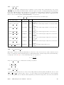
24 NOV 2005
Printed
First Release.
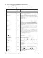
Update of the First Release. Section 6, Tables 61, 9, 11, 12,
15, 50, 56 and Figures 10, 28 were updated.
Section 12.9.1 was added.
Second Release.
Sections 5, 6, 8 and the bibliography were updated. Sections
12.9, 12.12.2, C.8, C.9.2 were added.
Third Release. Sections 6, 7 and 8 were updated. Sections
9.10, C.9.3 were added.
Fourth Release. Sections 6,7,8, and the bibliography were
updated.
Update of the Fourth Release. Sections 6, 8, Tables 15, 16,
and the bibliography were updated.
Fifth Release. Cookbook Part was completely rewritten.
All other parts were updated.
Minor update of the 5.0 version. Section 9.5 was added.
Sections 9.3.1, 9.4.1 and 9.7 were updated. Table 40 was
updated.
Update of the Fifth Release. Sections 7.1.2, 7.2,8.3,9.3.2,
9.9.2, 12.2, 12.9, 11, and the bibliography were updated.
Section 10.3, 12.9.2, and Table 53 were added.
ISDC – IBIS Analysis User Manual – Issue 5.1
ii
Contents
Acronyms and Abbreviations . . . . . . . . . . . . . . . . . . . . . . . . . . . . . . . . . . . . . . .
xii
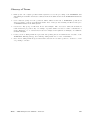
Glossary of Terms . . . . . . . . . . . . . . . . . . . . . . . . . . . . . . . . . . . . . . . . . . . . . xiii
1
I
Introduction . . . . . . . . . . . . . . . . . . . . . . . . . . . . . . . . . . . . . . . . . . . . . .
Instrument Definition
1
2
2
Scientific Performances Summary . . . . . . . . . . . . . . . . . . . . . . . . . . . . . . . . . .
3
3
Instrument Description . . . . . . . . . . . . . . . . . . . . . . . . . . . . . . . . . . . . . . . .
4
3.1
The Overall Design . . . . . . . . . . . . . . . . . . . . . . . . . . . . . . . . . . . . . .
4
3.2
The Subsystems . . . . . . . . . . . . . . . . . . . . . . . . . . . . . . . . . . . . . . .
7
3.2.1
The Mask
. . . . . . . . . . . . . . . . . . . . . . . . . . . . . . . . . . . . .
7
3.2.2
The Collimator . . . . . . . . . . . . . . . . . . . . . . . . . . . . . . . . . . .
8
3.2.3
Detector . . . . . . . . . . . . . . . . . . . . . . . . . . . . . . . . . . . . . .
8
3.2.4
On-board Calibration Unit . . . . . . . . . . . . . . . . . . . . . . . . . . . .
9
3.2.5
Veto Shield
. . . . . . . . . . . . . . . . . . . . . . . . . . . . . . . . . . . .
9
How the Instrument works . . . . . . . . . . . . . . . . . . . . . . . . . . . . . . . . . . . . . .
11
4.1
Event Types . . . . . . . . . . . . . . . . . . . . . . . . . . . . . . . . . . . . . . . . .
11
4.2
IBIS observing modes . . . . . . . . . . . . . . . . . . . . . . . . . . . . . . . . . . . .
12
4
II
Cookbook
14
5
Overview . . . . . . . . . . . . . . . . . . . . . . . . . . . . . . . . . . . . . . . . . . . . . . .
15
6
Getting started . . . . . . . . . . . . . . . . . . . . . . . . . . . . . . . . . . . . . . . . . . . .
18
6.1
. . . . . . . . . . . . . . . . . . . . . . . . . . . . . . . .
18
Downloading data from the archive . . . . . . . . . . . . . . . . . . . . . . .
19
6.2
Setting the environment . . . . . . . . . . . . . . . . . . . . . . . . . . . . . . . . . . .
20
6.3
Two ways of launching the analysis . . . . . . . . . . . . . . . . . . . . . . . . . . . . .
21
6.3.1
Graphical User Interface (GUI)
. . . . . . . . . . . . . . . . . . . . . . . . .
21
6.3.2
Launching scripts without GUI . . . . . . . . . . . . . . . . . . . . . . . . . .
21
Useful to know! . . . . . . . . . . . . . . . . . . . . . . . . . . . . . . . . . . . . . . . .
21
A Walk through ISGRI Analysis . . . . . . . . . . . . . . . . . . . . . . . . . . . . . . . . . .
23
7.1
Image Reconstruction . . . . . . . . . . . . . . . . . . . . . . . . . . . . . . . . . . . .
23
7.1.1
Results from the Image Step . . . . . . . . . . . . . . . . . . . . . . . . . . .
25
7.1.2
Displaying the Results from the Image Step
26
Setting up the analysis data
6.1.1
6.4
7
ISDC – IBIS Analysis User Manual – Issue 5.1
. . . . . . . . . . . . . . . . . .
iii
7.2
. . . . . . . . . . . . . . . . . . . . . . . . . . . . . . . . . . . . .
27
7.2.1
Results of the Spectral Extraction . . . . . . . . . . . . . . . . . . . . . . . .
31
7.2.2
Displaying the Results of the Spectral Extraction . . . . . . . . . . . . . . .
31
Lightcurve Extraction . . . . . . . . . . . . . . . . . . . . . . . . . . . . . . . . . . . .
32
7.3.1
Results of the Lightcurve Extraction . . . . . . . . . . . . . . . . . . . . . . .
33
7.3.2
Displaying the Results of the Lightcurve Extraction . . . . . . . . . . . . . .
33
More on ISGRI relevant parameters . . . . . . . . . . . . . . . . . . . . . . . . . . . . . . . .
34
8.1
How to choose the start and end level for the analysis . . . . . . . . . . . . . . . . . .
34
8.2
Imaging . . . . . . . . . . . . . . . . . . . . . . . . . . . . . . . . . . . . . . . . . . . .
35
8.2.1
How to choose the source search method in the Science Window analysis . .
35
8.2.2
Parameters related to the mosaic step
. . . . . . . . . . . . . . . . . . . . .
36
8.2.3
Background Subtraction
. . . . . . . . . . . . . . . . . . . . . . . . . . . . .
37
8.2.4
Miscellanea on Imaging . . . . . . . . . . . . . . . . . . . . . . . . . . . . . .
37
7.3
8
8.3
9
Spectral Extraction
Spectral and Timing Analysis
. . . . . . . . . . . . . . . . . . . . . . . . . . . . . . .
37
8.3.1
Spectral Energy Binning . . . . . . . . . . . . . . . . . . . . . . . . . . . . .
37
8.3.2
Background Subtraction . . . . . . . . . . . . . . . . . . . . . . . . . . . . . .
38
8.3.3
Input catalog . . . . . . . . . . . . . . . . . . . . . . . . . . . . . . . . . . . .
38
Useful recipes for the ISGRI data analysis
. . . . . . . . . . . . . . . . . . . . . . . . . . . .
39
9.1
Rerunning the Analysis . . . . . . . . . . . . . . . . . . . . . . . . . . . . . . . . . . .
39
9.2
Make your own Good Time Intervals . . . . . . . . . . . . . . . . . . . . . . . . . . . .
39
9.3
Combining results from different observation groups . . . . . . . . . . . . . . . . . . .
40
9.3.1
Creating a mosaic from different observation groups . . . . . . . . . . . . . .
40
9.3.2
Combining spectra and lightcurves from different observation groups
. . . .
41
. . . . . . . . . . . . . . . . . . . . . . . . . . . . . .
42
9.4
Rebinning the Response Matrix
9.4.1
Extracting images in more than 10 energy ranges
. . . . . . . . . . . . . . .
43
9.5
Some tricks on saving disk space and CPU time. . . . . . . . . . . . . . . . . . . . . .
43
9.6
Create your own catalog
. . . . . . . . . . . . . . . . . . . . . . . . . . . . . . . . . .
44
9.7
Alternative Spectral Extraction from the Mosaic . . . . . . . . . . . . . . . . . . . . .
44
9.8
Barycentrisation . . . . . . . . . . . . . . . . . . . . . . . . . . . . . . . . . . . . . . .
45
9.9
Alternative Timing Analysis . . . . . . . . . . . . . . . . . . . . . . . . . . . . . . . . .
45
9.9.1
ii light . . . . . . . . . . . . . . . . . . . . . . . . . . . . . . . . . . . . . .
45
9.9.2
Run ii light . . . . . . . . . . . . . . . . . . . . . . . . . . . . . . . . . . .
46
9.9.3
Merge the ii light results from different Science Windows . . . . . . . . . . .
46
ISDC – IBIS Analysis User Manual – Issue 5.1
iv
9.10
10
Timing Analysis without the deconvolution . . . . . . . . . . . . . . . . . . . . . . . .
PICsIT data analysis
. . . . . . . . . . . . . . . . . . . . . . . . . . . . . . . . . . . . . . . .
48
PICsIT Image Reconstruction . . . . . . . . . . . . . . . . . . . . . . . . . . . . . . . .
49
10.1.1
Results of PICsIT image analysis . . . . . . . . . . . . . . . . . . . . . . . . .
52
10.2
PICsIT spectral extraction from the mosaic image . . . . . . . . . . . . . . . . . . . .
52
10.3
PICsIT pipeline spectral extraction
. . . . . . . . . . . . . . . . . . . . . . . . . . . .
54
Displaying the results of PICsIT spectral analysis . . . . . . . . . . . . . . .
55
PICsIT Timing Analysis . . . . . . . . . . . . . . . . . . . . . . . . . . . . . . . . . . .
57
10.1
10.3.1
10.4
11
III
12
47
Known Limitations
. . . . . . . . . . . . . . . . . . . . . . . . . . . . . . . . . . . . . . . . .
58
11.1
ISGRI . . . . . . . . . . . . . . . . . . . . . . . . . . . . . . . . . . . . . . . . . . . . .
58
11.2
PICsIT . . . . . . . . . . . . . . . . . . . . . . . . . . . . . . . . . . . . . . . . . . . .
59
Data Analysis in Details
60
Science Analysis . . . . . . . . . . . . . . . . . . . . . . . . . . . . . . . . . . . . . . . . . . .
61
12.1
. . . . . . . . . . . . . . . . . . . . . . . . . . . . . . . . . . . . . . . .
61
12.1.1
ibis isgr evts tag . . . . . . . . . . . . . . . . . . . . . . . . . . . . . . . . . .
61
12.1.2
ibis isgr energy . . . . . . . . . . . . . . . . . . . . . . . . . . . . . . . . . .
61
12.1.3
ip ev correction . . . . . . . . . . . . . . . . . . . . . . . . . . . . . . . . . . .
64
ibis gti
. . . . . . . . . . . . . . . . . . . . . . . . . . . . . . . . . . . . . . . . . . . .
64
12.2.1
gti create . . . . . . . . . . . . . . . . . . . . . . . . . . . . . . . . . . . . . .
65
12.2.2
gti attitude . . . . . . . . . . . . . . . . . . . . . . . . . . . . . . . . . . . . .
65
12.2.3
gti data gaps . . . . . . . . . . . . . . . . . . . . . . . . . . . . . . . . . . . .
65
12.2.4
gti import . . . . . . . . . . . . . . . . . . . . . . . . . . . . . . . . . . . . . .
65
12.2.5
gti merge . . . . . . . . . . . . . . . . . . . . . . . . . . . . . . . . . . . . . .
66
. . . . . . . . . . . . . . . . . . . . . . . . . . . . . . . . . . . . . . . . . . .
66
12.3.1
ibis isgr deadtime . . . . . . . . . . . . . . . . . . . . . . . . . . . . . . . . .
67
12.3.2
ibis pics deadtime . . . . . . . . . . . . . . . . . . . . . . . . . . . . . . . . .
67
ibis binning . . . . . . . . . . . . . . . . . . . . . . . . . . . . . . . . . . . . . . . . . .
67
12.4.1
ii shadow build . . . . . . . . . . . . . . . . . . . . . . . . . . . . . . . . . . .
68
12.4.2
ip ev shadow build . . . . . . . . . . . . . . . . . . . . . . . . . . . . . . . . .
68
12.4.3
ip si shadow build . . . . . . . . . . . . . . . . . . . . . . . . . . . . . . . . .
69
12.5
ii map rebin . . . . . . . . . . . . . . . . . . . . . . . . . . . . . . . . . . . . . . . . . .
70
12.6
ibis background cor
70
12.2
12.3
12.4
ibis correction
ibis dead
. . . . . . . . . . . . . . . . . . . . . . . . . . . . . . . . . . . . .
ISDC – IBIS Analysis User Manual – Issue 5.1
v
12.7
12.6.1
ii shadow ubc . . . . . . . . . . . . . . . . . . . . . . . . . . . . . . . . . . . .
70
12.6.2
ip shadow ubc . . . . . . . . . . . . . . . . . . . . . . . . . . . . . . . . . . .
71
. . . . . . . . . . . . . . . . . . . . . . . . . . . . . . . . . . . . . . . . . . .
72
cat extract . . . . . . . . . . . . . . . . . . . . . . . . . . . . . . . . . . . . .
72
Image analysis . . . . . . . . . . . . . . . . . . . . . . . . . . . . . . . . . . . . . . . .
72
12.8.1
ii skyimage . . . . . . . . . . . . . . . . . . . . . . . . . . . . . . . . . . . . .
75
12.8.2
sumhist . . . . . . . . . . . . . . . . . . . . . . . . . . . . . . . . . . . . . . .
77
12.8.3
ip skyimage
. . . . . . . . . . . . . . . . . . . . . . . . . . . . . . . . . . . .
77
. . . . . . . . . . . . . . . . . . . . . . . . . . . . . . . . . . . . . .
77
Catalogs
12.7.1
12.8
12.9
Spectral Analysis
12.9.1
ii spectra extract
. . . . . . . . . . . . . . . . . . . . . . . . . . . . . . . . .
77
12.9.2
ip spectra extract
. . . . . . . . . . . . . . . . . . . . . . . . . . . . . . . . .
79
12.10 Timing Analysis . . . . . . . . . . . . . . . . . . . . . . . . . . . . . . . . . . . . . . .
79
12.10.1
ii lc extract . . . . . . . . . . . . . . . . . . . . . . . . . . . . . . . . . . . . .
79
12.10.2
ip st lc extract . . . . . . . . . . . . . . . . . . . . . . . . . . . . . . . . . . .
80
12.11 Summing up the results . . . . . . . . . . . . . . . . . . . . . . . . . . . . . . . . . . .
80
12.11.1
A
ip skymosaic . . . . . . . . . . . . . . . . . . . . . . . . . . . . . . . . . . . .
80
12.12 Tools not included in the pipeline . . . . . . . . . . . . . . . . . . . . . . . . . . . . . .
81
. . . . . . . . . . . . . . . . . . . . . . . . . . . . . . . . . . . .
81
12.12.2
ii light
. . . . . . . . . . . . . . . . . . . . . . . . . . . . . . . . . . . . . . .
82
. . . . . . . . . . . . . . . . . . . . . . . . . . . . . . .
84
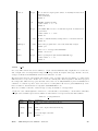
Raw Data . . . . . . . . . . . . . . . . . . . . . . . . . . . . . . . . . . . . . . . . . . .
84
A.1.1
Photon-by-photon mode . . . . . . . . . . . . . . . . . . . . . . . . . . . . . .
84
A.1.2
PICsIT Standard Mode . . . . . . . . . . . . . . . . . . . . . . . . . . . . . .
84
Prepared Data . . . . . . . . . . . . . . . . . . . . . . . . . . . . . . . . . . . . . . . .
85
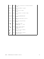
Instrument Characteristics used in Data Analysis. . . . . . . . . . . . . . . . . . . . . . . . .
86
B.1
Noisy Pixels
. . . . . . . . . . . . . . . . . . . . . . . . . . . . . . . . . . . . . . . . .
86
B.2
Calibration Corrections . . . . . . . . . . . . . . . . . . . . . . . . . . . . . . . . . . .
86
B.2.1
ISGRI . . . . . . . . . . . . . . . . . . . . . . . . . . . . . . . . . . . . . . . .
86
B.2.2
PICsIT . . . . . . . . . . . . . . . . . . . . . . . . . . . . . . . . . . . . . . .
87
B.3
Limit Tables . . . . . . . . . . . . . . . . . . . . . . . . . . . . . . . . . . . . . . . . .
87
B.4
Instrument Background . . . . . . . . . . . . . . . . . . . . . . . . . . . . . . . . . . .
87
A.2
C
mosaic spec
Low Level Processing Data Products
A.1
B
12.12.1
Science Data Products
C.1
ibis correction
. . . . . . . . . . . . . . . . . . . . . . . . . . . . . . . . . . . . . . .
89
. . . . . . . . . . . . . . . . . . . . . . . . . . . . . . . . . . . . . . . .
89
ISDC – IBIS Analysis User Manual – Issue 5.1
vi
C.2
ibis gti . . . . . . . . . . . . . . . . . . . . . . . . . . . . . . . . . . . . . . . . . . . .
89
C.3
ibis dead . . . . . . . . . . . . . . . . . . . . . . . . . . . . . . . . . . . . . . . . . . .
90
C.4
ibis binning
. . . . . . . . . . . . . . . . . . . . . . . . . . . . . . . . . . . . . . . . .
91
ii shadow build . . . . . . . . . . . . . . . . . . . . . . . . . . . . . . . . . . .
91
C.5
cat extract . . . . . . . . . . . . . . . . . . . . . . . . . . . . . . . . . . . . . . . . . .
91
C.6
ibis background cor . . . . . . . . . . . . . . . . . . . . . . . . . . . . . . . . . . . . .
92
C.7
Image Analysis . . . . . . . . . . . . . . . . . . . . . . . . . . . . . . . . . . . . . . . .
92
C.7.1
. . . . . . . . . . . . . . . . . . . . . . . . . . . . . . . . . . . .
92
ip skyimage . . . . . . . . . . . . . . . . . . . . . . . . . . . . . . . . . . . .
95
C.4.1
C.7.2
C.8
Spectral Analysis
C.8.1
C.9
D
ii skyimage
. . . . . . . . . . . . . . . . . . . . . . . . . . . . . . . . . . . . . .
ii spectra extract
95
. . . . . . . . . . . . . . . . . . . . . . . . . . . . . . . . .
95
Timing Analysis . . . . . . . . . . . . . . . . . . . . . . . . . . . . . . . . . . . . . . .
96
C.9.1
96
ip st lc extract . . . . . . . . . . . . . . . . . . . . . . . . . . . . . . . . . . .
C.9.2
ii lc extract
. . . . . . . . . . . . . . . . . . . . . . . . . . . . . . . . . . . .
C.9.3
Timing Analysis without the deconvolution
List of ibis science analysis parameters
96
. . . . . . . . . . . . . . . . . .
96
. . . . . . . . . . . . . . . . . . . . . . . . . . . . . .
98
ISDC – IBIS Analysis User Manual – Issue 5.1
vii
List of Figures
1
IBIS effective area . . . . . . . . . . . . . . . . . . . . . . . . . . . . . . . . . . . . . . . . . .
4
2
Cutaway drawing of the IBIS detector assembly, together with the lower part of the collimator
(Hopper). . . . . . . . . . . . . . . . . . . . . . . . . . . . . . . . . . . . . . . . . . . . . . . .
5
3
IBIS detector assembly in numbers. . . . . . . . . . . . . . . . . . . . . . . . . . . . . . . . . .
5
4
Spacecraft & Instrument Coordinate Systems. . . . . . . . . . . . . . . . . . . . . . . . . . . .
6
5
The IBIS coded mask pattern.
. . . . . . . . . . . . . . . . . . . . . . . . . . . . . . . . . . .
7
6
The cross section of the support panel. . . . . . . . . . . . . . . . . . . . . . . . . . . . . . . .
8
7
ISGRI and PICsIT division in modules and submodules . . . . . . . . . . . . . . . . . . . . .
9
8
The schematic view of PICsIT layer. . . . . . . . . . . . . . . . . . . . . . . . . . . . . . . . .
10
9
IBIS sensitivities for the various detection techniques. . . . . . . . . . . . . . . . . . . . . . .
12
10
Science Analysis Overview . . . . . . . . . . . . . . . . . . . . . . . . . . . . . . . . . . . . . .
15
11
Structure of the directory created with og create . . . . . . . . . . . . . . . . . . . . . . . . .
23
12
Main page of the IBIS GUI . . . . . . . . . . . . . . . . . . . . . . . . . . . . . . . . . . . . .
24
13
Imaging page of IBIS GUI
. . . . . . . . . . . . . . . . . . . . . . . . . . . . . . . . . . . . .
25
14
Overview of the IMA level products . . . . . . . . . . . . . . . . . . . . . . . . . . . . . . . .
26
15
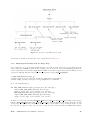
Sketch of the isgri sky ima.fits structure (left), and extract from the Index table (right).
. .
27
16
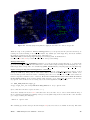
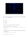
Intensity (left) and significance (right) mosaic in the 20 – 40 keV energy band
. . . . . . . .
28
17
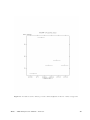
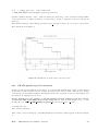
4U 1700-377 science window per science window lightcurve in the 20 – 40 keV energy band .
29
18
Page of IBIS GUI for Spectral and Ligtcurve extraction . . . . . . . . . . . . . . . . . . . . .
30
19
List of sources used for spectral analysis . . . . . . . . . . . . . . . . . . . . . . . . . . . . . .
30
20
Total 4U 1700-377 spectrum. . . . . . . . . . . . . . . . . . . . . . . . . . . . . . . . . . . . .
32
21
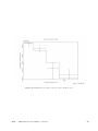
4U1700-377.fits lightcurve in 20 – 40 keV energy range with 100 sec binning. . . . . . . . . .
34
22
Crab power spectrum. . . . . . . . . . . . . . . . . . . . . . . . . . . . . . . . . . . . . . . . .
49
23
Main page of the IBIS GUI . . . . . . . . . . . . . . . . . . . . . . . . . . . . . . . . . . . . .
50
24
PICsIT page of the IBIS GUI
51
25
Crab significance image in the 252 − 336 keV energy band as seen by PICsIT.
. . . . . . . .
53
26
PICsIT Crab spectrum extracted from the mosaic. . . . . . . . . . . . . . . . . . . . . . . . .
54
27
PICsIT Crab spectrum created as described in Section 10.3.
. . . . . . . . . . . . . . . . . .
56
28
Composition of the main script ibis science analysis. For further descriptions of the BIN BKG
steps for the DEAD, IMA and BIN S levels, see Figures 29, 30 and 31 respectively. . . . . . . . .
62
29
Overview of the binning - background step for Imaging. . . . . . . . . . . . . . . . . . . . . .
63
30
Overview of the binning - background step for Spectra. . . . . . . . . . . . . . . . . . . . . . .
63
31
Overview of the binning - background step for Lightcurves. . . . . . . . . . . . . . . . . . . .
63
. . . . . . . . . . . . . . . . . . . . . . . . . . . . . . . . . . .
ISDC – IBIS Analysis User Manual – Issue 5.1
viii
32
SPSF for the IBIS/ISGRI telescope. . . . . . . . . . . . . . . . . . . . . . . . . . . . . . . . .
ISDC – IBIS Analysis User Manual – Issue 5.1
74
ix
List of Tables
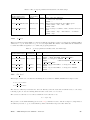
1
Scientific Parameters of IBIS. . . . . . . . . . . . . . . . . . . . . . . . . . . . . . . . . . . . .
2
Characteristics of the IBIS Telemetry Formats
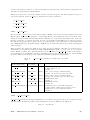
3
ibis isgr evts tag parameters included into the main script.
. . . . . . . . . . . . . . . . . . .
61
4
ibis isgr energy parameters included into the main script. . . . . . . . . . . . . . . . . . . . .
64
5
ip ev correction parameters included into the main script. . . . . . . . . . . . . . . . . . . . .
64
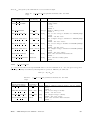
6
gti create parameters included into the main script. . . . . . . . . . . . . . . . . . . . . . . .
65
7
gti attitude parameters included into the main script. . . . . . . . . . . . . . . . . . . . . . .
65
8
. . . . . . . . . . . . . . . . . . . . . . . . . .
13
. . . . . . . . . . . . . . . . . . . .
66
9
gti merge parameters included into the main script. . . . . . . . . . . . . . . . . . . . . . . .
66
10
ibis isgr deadtime parameters included into the main script.
. . . . . . . . . . . . . . . . . .
67
11
ii shadow build parameters included into the main script.
. . . . . . . . . . . . . . . . . . .
68
12
ip ev shadow build parameters included into the main script. . . . . . . . . . . . . . . . . . .
69
13
ip si shadow build parameters included into the main script. . . . . . . . . . . . . . . . . . .
69
14
ii map rebin parameters included into the main script.
. . . . . . . . . . . . . . . . . . . . .
70
15
ii shadow ubc parameters included into the main script.
. . . . . . . . . . . . . . . . . . . .
71
16
ip shadow ubc parameters included into the main script.
. . . . . . . . . . . . . . . . . . . .
71
. . . . . . . . . . . . . . . . . . . . . .
72
18
ii skyimage parameters included into the main script. . . . . . . . . . . . . . . . . . . . . . .
75
19
sumhist parameters included into the main script. . . . . . . . . . . . . . . . . . . . . . . . .
77
20
ip skyimage parameters included into the main script.
. . . . . . . . . . . . . . . . . . . . .
77
21
ii spectra extract parameters included into the main script. . . . . . . . . . . . . . . . . . . .
78
22
ip spectra extract parameters included into the main script.
. . . . . . . . . . . . . . . . . .
79
17
The gti import parameters included into the main script.
3
cat extract parameters included into the main script.
23
Parameters for the ii lc extract.
. . . . . . . . . . . . . . . . . . . . . . . . . . . . . . . . . .
79
24
Parameters for the ip st lc extract. . . . . . . . . . . . . . . . . . . . . . . . . . . . . . . . . .
80
25
ip skymosaic parameters included into the main script.
. . . . . . . . . . . . . . . . . . . . .
80
26
mosaic spec parameters.
. . . . . . . . . . . . . . . . . . . . . . . . . . . . . . . . . . . . . .
81
27
ii light parameters.
. . . . . . . . . . . . . . . . . . . . . . . . . . . . . . . . . . . . . . . . .
82
28
List of IBIS ****-****-RAW Data Structures . . . . . . . . . . . . . . . . . . . . . . . . . . .
84
29
Contest of Photon-by-Photon Mode Raw Data.
. . . . . . . . . . . . . . . . . . . . . . . . .
84
30
Content of PICS-SPTI-RAW Data Structure.
. . . . . . . . . . . . . . . . . . . . . . . . . .
85
31
Content of ISGR-SWIT-STA Data Structure . . . . . . . . . . . . . . . . . . . . . . . . . . .
86
32
Content of PICS-FALT-STA Data Structure
86
ISDC – IBIS Analysis User Manual – Issue 5.1
. . . . . . . . . . . . . . . . . . . . . . . . . . .
x
33
Content of ISGR-RISE-MOD Data Structure . . . . . . . . . . . . . . . . . . . . . . . . . . .
86
34
Content of ISGR-OFFS-MOD Data Structure
. . . . . . . . . . . . . . . . . . . . . . . . . .
87
35
Content of PICS-ENER-MOD Data Structure
. . . . . . . . . . . . . . . . . . . . . . . . . .
87
36
Content of IBIS-GOOD-LIM limit table. . . . . . . . . . . . . . . . . . . . . . . . . . . . .
87
37
Instrument Background Model Data Structures.
. . . . . . . . . . . . . . . . . . . . . . . . .
87
38
Content of Indexes for Table 37 Data Structures.
. . . . . . . . . . . . . . . . . . . . . . . .
88
39
List of Data Structures produced at COR level . . . . . . . . . . . . . . . . . . . . . . . . . .
89
40
Content the level COR Data Structures for the photon-by-photon mode.
. . . . . . . . . . .
89
41
Content the PICS-SISH-COR-IDX Data Structure.
. . . . . . . . . . . . . . . . . . . . . . .
89
42
Content of IBIS-GNRL-GTI Data Structures. . . . . . . . . . . . . . . . . . . . . . . . . .
89
43
Content of ISGR-DEAD-SCP Data Structures.
. . . . . . . . . . . . . . . . . . . . . . . .
90
44
Content of PICS-DEAD-SCP Data Structures.
. . . . . . . . . . . . . . . . . . . . . . . .
90
45
Content of COMP-DEAD-SCP Data Structures.
. . . . . . . . . . . . . . . . . . . . . . .
90
46
List of Data Structures produced at BIN level
. . . . . . . . . . . . . . . . . . . . . . . . . .
91
47
Content of ****-****-SHD-IDX Data Structures. . . . . . . . . . . . . . . . . . . . . . . .
91
48
Content of GNRL-REFR-CAT Data Structures.
. . . . . . . . . . . . . . . . . . . . . . . . .
91
49
Content of ISGR-SKY.-IMA-IDX Data Structure. . . . . . . . . . . . . . . . . . . . . . .
93
50
Content of ISGR-SKY.-RES Data Structure.
93
51
Content of ISGR-SKY.-RES-IDX Data Structure.
52
New information added to the ISGR-SRCL-RES Data Structure.
53
Content of the ISGR-OBS.-RES Data Structure.
. . . . . . . . . . . . . . . . . . . . . . . . .
. . . . . . . . . . . . . . . . . . . . . .
93
. . . . . . . . . . . . . .
94
. . . . . . . . . . . . . . . . . . . . . . .
94
54
Content of the ISGR-EVTS-SPE Data Structure. . . . . . . . . . . . . . . . . . . . . . . .
95
55
Content of the ISGR-EVTS-SPE-IDX Data Structure. . . . . . . . . . . . . . . . . . . . .
95
56
Content of the PICS-EVTS-LCR-IDX Data Structure.
. . . . . . . . . . . . . . . . . . .
96
57
Content of the PICS-EVTS-LCR Data Structure. . . . . . . . . . . . . . . . . . . . . . . .
96
58
Content of the ISGR-SRC.-LCR-IDX Data Structure. . . . . . . . . . . . . . . . . . . . .
96
59
Content of the GNRL-EVTS-LST Data Structure. . . . . . . . . . . . . . . . . . . . . . .
97
60
Content of the GNRL-EVTS-GTI Data Structure. . . . . . . . . . . . . . . . . . . . . . .
97
61
ibis science analysis parameters description. . . . . . . . . . . . . . . . . . . . . . . . . . . . .
98
ISDC – IBIS Analysis User Manual – Issue 5.1
xi
Acronyms and Abbreviations
AD
Architectural Design
HEPI
Hardware Event Processor
ADD
Architectural Design Document
HV
High Voltage
A/D
Analog-Digital
IC
Instrument Characteristics
AFEE
Analog Front End Electronics
IJD
Integral Julian Day
ASIC
Application Specific Integrated Circuits
ISDC
Integral Science Data Center
BGO
Bismuth Germanate
ISOC
Integral Science Operations Centre
CdTe
Cadmium-Telluride
MCE
Module Control Electronics
CsI
Caesium-Iodide
MDU
Modular Detection Units
DBB
Detector Bias Box
OBT
On-Board Time
DFEE
Digital Front End Electronics
OG
Observation Group
DOL
Data Object Locator
PCFOV
Partially Coded Field of View
DPE
Data Processing Electronics
PEB
PICsIT Electronic Box
DS
Data Structure
PIF
Pixel Illuminated Factor
FCFOV
Fully Coded Field of View
PMT
Photomultiplier Tube
FIFO
First-In, First-Out
PLM
Payload Module
FOV
Field of View
RMF
Redistribution Matrix Files
FWHM
Full Width at Half Maximum
ScW
Science Window
GPS
Galactic Plane Scan
SWG
Science Window Group
GTI
Good Time Interval
TBW
To be written
GUI
Graphical User Interface
TM
Telemetry
ISDC – IBIS Analysis User Manual – Issue 5.1
xii
Glossary of Terms
• ISDC system: the complete ground software system devoted to the processing of the INTEGRAL data
and running at the ISDC. It includes contributions from the ISDC and from the INTEGRAL instrument
teams.
• Science Window (ScW): For the operations, ISDC defines atomic bits of INTEGRAL operations as
either a pointing or a slew, and calls them ScWs. A set of data produced during a ScW is a basic piece
of INTEGRAL data in the ISDC system.
• Observation: Any group of ScW used in the data analysis. The observation defined from ISOC in
relation with the proposal is only one example of possible ISDC observations. Other combinations of
Science Windows, i.e., of observations, are used for example for the Quick-Look Analysis, or for Off-Line
Scientific Analysis.
• Pointing: Period during which the spacecraft axis pointing direction remains stable. Because of the
INTEGRAL dithering strategy, the nominal pointing duration is of order of 20 minutes.
• Slew: Period during which the spacecraft is manoeuvred from one stable position to another, i.e., from
one pointing to another.
ISDC – IBIS Analysis User Manual – Issue 5.1
xiii
1
Introduction
The ’IBIS Analysis User Manual’, i.e., this document, was edited to help you with the IBIS specific part of
the INTEGRAL Data Anaysis.
A more general overview on the INTEGRAL Data Analysis can be found in the ’Introduction to the INTEGRAL Data Analysis’ [1]. For the ISGRI and PICsIT analysis scientific validation reports see [3] and
[4].
The ’IBIS Analysis User Manual’ is divided into two major parts:
• Description of the Instrument
This part, based to some extent on the ISOC AO-2 document [2], introduces the INTEGRAL on-board
Imager (IBIS).
• Description of the Data Analysis
This part starts with an overview describing the different steps of the analysis. Then, in the Cookbook
Section, several examples of analysis and their results and the description of the parameters are given.
Finally, the used algorithms are described. A list of the known limitations of the current release is also
provided.
In the Appendix of this document you find the description of the Raw and Prepared Data and also the
description of the Scientific Products. If you are interested in Data Structures not described in the Appendix
go to the ISDC web-page http://isdc.unige.ch/index.cgi?Data+templates
ISDC – IBIS Analysis User Manual – Issue 5.1
1
Part I
Instrument Definition
ISDC – IBIS Analysis User Manual – Issue 5.1
2
2
Scientific Performances Summary
IBIS is a gamma-ray telescope observing celestial objects of all classes ranging from the most compact galactic
systems to extragalactic objects, with powerful diagnostic capabilities of fine imaging, source identification
and spectral sensitivity in both continuum and lines. It is able to localize weak sources at low energy to
better than a few arcminutes accuracy, covering the entire energy range from a few tens of keV to several
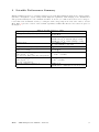
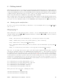
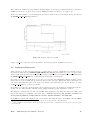
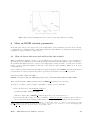
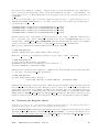
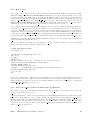
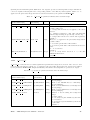
MeV. Table 1 gives an overview of the scientific capabilities of IBIS. The effective area curves are given on
the Figure 1.
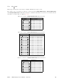
Table 1: Scientific Parameters of IBIS.
Operating energy range
Energy resolution (FWHM)
Effective Area
Field of view
Angular resolution (FWHM)
Point source location accuracy
(90% error radius)
Continuum sensitivity,
photons cm−2 s−1 keV−1
(3σ detection, ∆E = E/2, 106 s integration)
Narrow line sensitivity,
photons cm−2 s−1
(3σ, 106 s integration)
Absolute timing accuracy (3 σ)
ISDC – IBIS Analysis User Manual – Issue 5.1
15 keV – 10 MeV
7% @ 100 keV
9% @ 1 MeV
ISGRI: 960 cm2 at 50 keV
PICsIT: 870 cm2 at 300 keV (single events)
PICsIT: 275 cm2 at 1 MeV (multiple events)
9◦ × 9◦ (fully coded)
19◦ × 19◦ (partially coded, 50%)
120
3000 @100 keV
<50 @1 MeV
3.8 × 10−7 @100 keV
1 – 2×10−7 @ 1 MeV
1.3 × 10−5 @100 keV
4 × 10−5 @ 1 MeV
ISGRI: 61 µs
PICsIT: 0.976 – 500ms (selected from ground)
3
Figure 1: IBIS effective area
3
3.1
Instrument Description
The Overall Design
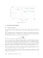
IBIS is a gamma-ray imager operating in the energy range 20 keV to 10 MeV, with two simultaneously
operating detectors covering the full energy range, located behind a Tungsten mask which provides the
encoding.
The coded mask is optimized for high angular resolution. As diffraction is negligible at gamma-ray wavelengths, the angular resolution of a coded-mask telescope is limited by the spatial resolution of the detector
array. The angular resolution of a coded mask telescope dθ is defined by the ratio between the mask element
size C (11.2 mm) and the mask-to-detection plane distance H (3133 mm).
C
dθ = arctan
= 120
H
IBIS is made of a large number of small, fully independent pixels.
The detector features two layers, ISGRI and PICsIT: the first is made of Cadmium-Telluride (CdTe) solidstate detectors and the second of Caesium-Iodide (CsI) scintillator crystals. This configuration ensures a
good broad line and continuum sensitivity over the wide spectral range covered by IBIS. The double-layer
discrete-element design of IBIS allows the paths of interacting photons to be tracked in 3D if the event
involves detection units of both ISGRI and PICsIT. The application of Compton reconstruction algorithms
to these types of events (between few hundred keV and few MeV) allows an increase in signal to noise ratio
attainable by rejecting those events unlikely to correspond to source photons inside the field of view.
The detector aperture is restricted, in the hard X-ray part of the spectrum, by passive shielding covering the
distance between mask and detection plane. An active BGO scintillator VETO system shields the detector
bottom as well as the four sides up to the bottom of ISGRI.
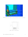
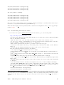
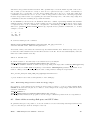
Figure 2 shows a cut-away drawing of the various components of IBIS (except the mask and tube). Figure
3 shows the distances between the different parts of the detector assembly. Figure 4 shows the spacecraft &
instruments coordinate systems.
ISDC – IBIS Analysis User Manual – Issue 5.1
4
Figure 2:
Cutaway drawing of the IBIS detector assembly, together with the lower part of the collimator (Hopper).
Figure 3: IBIS detector assembly in numbers.
ISDC – IBIS Analysis User Manual – Issue 5.1
5
Figure 4:
Spacecraft & Instrument Coordinate Systems. Note that the X-axis of the spacecraft is defined by the
pointing direction.
ISDC – IBIS Analysis User Manual – Issue 5.1
6
3.2
3.2.1
The Subsystems
The Mask
The IBIS Mask Assembly is rectangular with external dimensions of 1180 × 1142 × 114 mm3 , and consists of
three main subsystems: the Coded Pattern, the Support Panel and the Peripheral Frame with the necessary
interface provisions.
The Coded Pattern is a square array of size 1064 × 1064 × 16 mm3 , made up of 95×95 individual square
cells of size 11.2× 11.2 mm2 . The mask chosen for IBIS is based on a cyclic replication of MURA (Modified
Uniformly Redundant Array) of order 53. The properties of the MURA patterns are described e.g. in [11]
and [12].
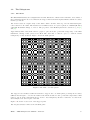
Approximately half of the mask cells are opaque to photons in the operational energy range of the IBIS
instrument, offering a 70% opacity at 1.5 MeV. The other 50% of cells are open, i.e., with an off-axis
transparency of 60% at 20 keV. Figure 5 shows the mask pattern.
Figure 5: The IBIS coded mask pattern.
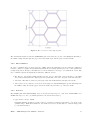
The Support Panel includes additional elements to support the code mask pixels, providing the necessary
stiffness and strength to overcome the launch environment and the in-orbit operational temperatures. This
panel is done from the material known as ”nomex”. Its transparency should be taken into account in the
data analysis, as it absorbs part of the flux.
Figure 6 shows the cross section of the support panel.
The Peripheral Frame reinforces the sandwich panel.
ISDC – IBIS Analysis User Manual – Issue 5.1
7
Figure 6: The cross section of the support panel.
The mechanical interfaces with the INTEGRAL payload module also provide extra Tungsten shielding to
the diffuse background through the gap between the mask edges and the payload vertical walls.
3.2.2
The Collimator
In order to maintain the low energy response of IBIS despite the dithering needed for SPI, the collimation
baseline consists of a passive lateral shield that limits the solid angle (and therefore the cosmic gamma-ray
background) viewed directly by the IBIS detector in the full field of view up to a few hundreds of keV. The
tube collimation system is implemented with three different devices:
• The Hopper : four inclined walls starting from the detector unit with a direct interface to the IBIS
detector mechanical structure. The hopper is not physically connected to the payload module structure.
• The Tube: The Tube is formed by four payload module walls shielded with glued Lead foils.
• The additional side shielding on the mask. Four strips of 1 mm thick Tungsten provide shielding from
the diffuse background in the gaps between the mask edges and the top of the tube walls.
3.2.3
Detector
The ISGRI CdTe and PICsIT CsI(Tl) detectors are layered with respect to each other, with PICsIT below
ISGRI with respect to the coded mask (and hence the astronomical source).
• Upper Detector Layer: ISGRI
Cadmium Telluride (CdTe) is a semiconductor operating at ambient temperature. 0◦ ± 20◦ C is the
optimum range. With their small area, the CdTe detectors are ideally suited to build an image with
good spatial resolution.
ISDC – IBIS Analysis User Manual – Issue 5.1
8
Figure 7: ISGRI and PICsIT division in modules and submodules
The CdTe layer is made of 8 identical Modular Detection Units each having 32×64 pixels (see Figure
7). Total sensitive area of the detector is 2621 cm2 .
• Lower Detector Layer: PICsIT
Caesium Iodide is a scintillation crystal. The CsI(Tl) layer is divided into eight rectangular modules of
16×32 detector elements (see Figure 7). In each module there are two independent semi-module each
one with its independent Front End Electronics. Total sensitive area of the detector is 2994 cm2 .
• Noisy Pixels
It is possible that with the time some of the pixels of the detector may become out of order and start
to produce outputs not triggered by an income photon, i.e., to become “noisy”. If the particular pixel
countrate is too high relatively to the module countrate, then the on-board electronics switch it off.
In ISGRI case the noisy pixels can recover after being switched off for some time and disabled pixels
are periodically reset to check their status.
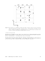
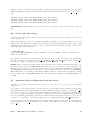
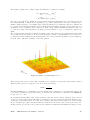
In PICsIT case, pixels cannot be recovered that easily. PICsIT pixel will remain off once killed. Only if
half of the detector (or so) will be off, an attempt will be made to turn pixels on. The current situation
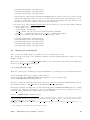
is shown on Figure 8. Overall the killed pixels are less than 1%.
3.2.4
On-board Calibration Unit
IBIS contains an on-board collimated radioactive 22 Na source. This allows regular calibration of PICsIT at
both the 511 keV line (calibration to better than 1% in 4 hours) and 1275 keV (1% in 8 hours). ISGRI can
also use the 511 keV line, albeit at lower efficiency. Any energy deposits from untagged photons will have
an impact of < 1% on the overall continuum sensitivity between 100 keV and 2 MeV.
3.2.5
Veto Shield
The Veto shield is crucial to the operation of IBIS. IBIS uses anticoincidence logic to accept or reject
detected events as real photons in the field of view, or background particles or photons propagating through,
ISDC – IBIS Analysis User Manual – Issue 5.1
9
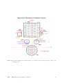
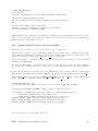
Figure 8:
The schematic view of PICsIT layer. Each module number is indicated. The dotted lines represents the
division in semimodules whose number is indicated at the top. The black pixel are the killed ones. The
(Y ,Z) coordinates are the IBIS ones both ranging from 0 to 63. X-axis is directed toward the source
located above the page. The Z-axis is pointing positively to the sun.
or induced in, the spacecraft.
The sides, up to the ISGRI bottom level, and rear of the stack of detector planes are surrounded by an active
Bismuth Germanate (BGO) veto shield. Like the detector array, the Veto shield is modular in construction.
There are 8 lateral shields, i.e., 2 modules per side, and 8 bottom modules.
The high density and mean Z of BGO ensures that a thickness of 20 mm is sufficient to reduce the detector
background due to leakage through the shielding of cosmic diffuse gamma-ray background and gamma-rays
produced in the spacecraft, to less than the sum of all other background components.
ISDC – IBIS Analysis User Manual – Issue 5.1
10
4
How the Instrument works
4.1
Event Types
The photon entering the telescope can be detected due to its interaction with the absorbing material of
the detector. Three major types of interactions play a dominant role: photoelectric absorption, Compton
scattering and pair production. In the photoelectric absorption process a photon undergoes an interaction
with an absorber atom in which the photon completely disappears. In its place an energetic photoelectron is
ejected by the atom, carrying away most of the original photon energy. The Compton scattering takes place
between the incident gamma-ray photon and an electron in the absorbing material. The incoming photon
is deflected and it transfers a portion of its energy to the electron. The energy transferred to the electron
can vary from zero to a large fraction of the initial gamma-ray energy. In the pair production process the
gamma-ray photon disappears and is replaced by an electron-positron pair. The positron will annihilate in
the absorbing medium and two annihilation photons are normally produced as secondary products of the
interaction. Depending on the size of the detector and on the energy of the incoming photon, a photon
scattered in a Compton interaction can escape the detector, or undergo a second interaction. The pairs
of 511 keV photons, produced by the annihilation of the positrons resulting from pair creation, can also
produce other interactions or escape the detector.
Both ISGRI and PICsIT record the coordinates of each event registered in the corresponding layer, to build
up an image. The anticoincidence VETO is used to reject background events.
The coded mask produces a shadowgram. Photons from the source and the background are distributed
across the entire field of view, but cross-correlation techniques allow the full image to be reconstituted for
the fully coded field of view (9◦ ×9◦ ) at each pointing. For the partially coded field of view (out to 29◦ ×
29◦ ), special cleaning techniques must be applied to the data to properly reconstruct the image. The actual
sky coverage in an observation of course depends on the dither pattern.
The on-board electronics classify registered events according to the activated layer and the number of events
detected by a submodule practically simultaneously. Events detected by different submodules are treated as
independent ones. There are five main events type:
• ISGRI single event
Photon is stopped in a single pixel of the ISGRI layer, generating an electric pulse.
In principle, the amplitude of the pulse yields the energy of the incident photon. However, above 50
keV the energy is a function of not just the pulse height but also the pulse rise time, so both are used to
determine the energy of the incident photon. In addition the resulting line profile (energy resolution) is
no longer Gaussian, but more similar to a Lorentzian. The energy resolution depends on the operating
temperature, and also on the bias voltage; the bias voltage has to be optimized as a trade-off between
high resolution but more noise (high voltage) or lower noise but lower resolution (low voltage).
All cases of multiple ISGRI detection units excitation (in one module) are rejected. In case of the
excitation of the detection units in different modules, such events are treated as independent single
events.
• PICsIT single event
Photon passes through ISGRI and is stopped in a single pixel of the PICsIT layer, generating one
scintillation flash.
The energy of the incident photon is derived, in each crystal bar, from the intensity of the flash recorded
in the photodiode. The energy resolution of PICsIT is a function of the signal-to-noise of the event,
which in turn is governed by factors operating conditions and PIN capacity.
• PICsIT multiple event
Several PICsIT detection units in one submodule were excited during one event, generating several
scintillation flashes. The energy of the primary photon is determined from the sum of the energies
of all detected events. The position of the incoming photon is attributed to the position of the most
energetic event.
ISDC – IBIS Analysis User Manual – Issue 5.1
11
• Compton single event Photons arriving in either ISGRI or PICsIT produce secondary photon via
Compton scattering, detected in another layer. The position of the incoming photon is attributed to
the position of the most energetic event, and the energy is determined as the sum of the detected
events energies.
• Compton multiple event
One ISGRI detection unit and several PICsIT detection units in one submodule were excited. As in
previous cases the position of the incoming photon is attributed to the position of the most energetic
event, and the energy is determined as the sum of the detected events energies.
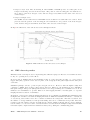
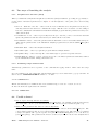
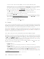
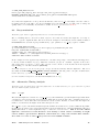
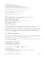
In Fig.9 the efficiencies of the various detection techniques is shown.
Figure 9: IBIS sensitivities for the various detection techniques.
4.2
IBIS observing modes
IBIS has several observing modes, for engineering and calibration purposes. However, for scientific use there
is only one operating mode, Science Mode.
In Science Mode, ISGRI registers and transmits events on a photon-by-photon basis, i.e., every event is
tagged with (X,Y ) position on the detector plane, event energy (from the pulse height and rise time) and
event time.
PICsIT in principle can also operate in photon-by-photon mode. However, with the higher background
compared to ISGRI, there would be unacceptable data loss. Therefore, the standard mode for PICsIT is
histogram. Images and spectra (full spatial resolution, 256 energy channels) are accumulated for about 30
minutes before transmission to ground. There is no time-tagging internal to the histogram, i.e., spectral
imaging has time resolution of 30 minutes.
In addition, coarse spectra, without imaging information, are accumulated by PICsIT and transmitted with
far higher time resolution, but without imaging information. Thus their usefulness is limited to observations
of very strong sources where the source countrate dominates the background. The time resolution, and
the number of energy channels, for this spectral timing data can be commanded from ground. The time
resolution can take values between 1 and 500 ms; the current default is 500 ms and two energy channels,
but the values to be used for routine observations will be decided when the in-flight background of PICsIT
is measured (and compared with the available telemetry rate), during the commissioning phase.
ISDC – IBIS Analysis User Manual – Issue 5.1
12
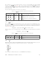
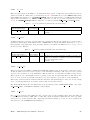
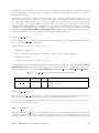
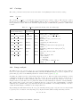
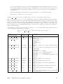
In Table 2 the properties of the all modes are summarized.
Table 2: Characteristics of the IBIS Telemetry Formats
Observing Mode
photon-by-photon
Photon-by-Photon
Spectral-Imaging
Spectral-Timing
Detector Image
Resolution
(pixels)
ISGRI
128×128
PICsIT
64×64
64×64
None
ISDC – IBIS Analysis User Manual – Issue 5.1
Timing
Resolution
Spectral
Resolution
(channels)
61.035µs
2048
64µs
≤ ∼30 min
1 – 500ms
1024
256
2–8
13
Part II
Cookbook
This Part was completely rewritten by
M.Chernyakova
A.Paizis
I. Lecoeur-Taibi
ISDC – IBIS Analysis User Manual – Issue 5.1
14
5
Overview
In this Section an overview of the analysis of IBIS data is given.
Each photon detected by IBIS is analyzed with the on-board electronics and tagged with the arrival time,
type (ISGRI , PICsIT, Compton1 etc.), energy, position etc. according to the operation mode (i.e. photonby-photon, standard, calibration etc.). These data are then sent to ground in telemetry (TM) packets.
During Pre-Processing the TM packet information is deciphered and rewritten into the set of FITS files
(RAW data). Then the local on-board time is converted into the common on-board time (OBT) and the
House Keeping (HK) parameters into physical units (PRP data).
These steps are done at ISDC and you do not have to redo them. In the Appendix you will find the
description of the raw and prepared data and also the description of the instrument characteristic files that
are used in the Scientific Analysis.
INTEGRAL data is organized into the so-called Science Windows (see Introduction to the INTEGRAL Data
Analysis [1] for more explanations). During the scientific analysis, all the Science Windows belonging to the
same observation are grouped together to form the ”Observation Group”.
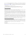
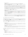
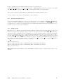
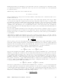
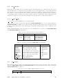
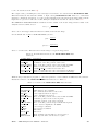
Figure 10 shows in details the different steps performed by the scientific analysis script, ibis science analysis.
This high level script consists of three smaller ones: ibis scw1 analysis, ibis obs1 analysis and ibis scw2 analysis.
ibis scw1 analysis and ibis scw2 analysis work on a Science Window basis while ibis obs1 analysis works on
the Observation Group basis. Each subscript performs the tasks shown in Figure 10, explained in more
details in the text below.
Figure 10: Science Analysis Overview
1 For
the time being, Compton analysis is not available
ISDC – IBIS Analysis User Manual – Issue 5.1
15
• The first script ibis scw1 analysis performs the following tasks:
COR – Data Correction
Tags noisy pixels, corrects energy of the photons for rise time and temporal variations of the gain,
transforms channels to energy. See Section 12.1 for more details.
GTI – Good Time Handling
Generates, selects, and merges Good Time Intervals (GTI) to produce a unique GTI that is then used
by the software to select good events. See Section 12.2 for more details.
DEAD – Dead Time Calculation
Calculates the total dead time during which the incoming photons may be lost due to the processing
of the previous events. Also veto strobe signals generated by BGO (Bismuth Germanate) shield,
calibration source and Compton events are taken into account. See Section 12.3 for more details.
BIN I – Event Binning for Imaging
Sorts data into energy bins. For each energy range, the intensity shadowgram and a corresponding
efficiency map are created. See Section 12.4 for more details.
BKG I – Background Correction
Creates rebinned maps for background and absorption of support mask (see Section 3.2.1) corrections.
Corrects for efficiency and subtracts background. See Section 12.6 for more details.
After these steps the high-level analysis is performed.
• The second script ibis obs1 analysis takes the whole Observation Group previously created as input
and performs the following tasks:
CAT I - Catalog Source Selection for Imaging
Selects from the given catalog a list of sources in the Field of View matching the criteria defined by
script parameters, and creates an output list with location and expected flux values of the selected
sources. See Section 12.7 for more details.
IMA - ISGRI and PICsIT (staring) Image Reconstruction
In the case of ISGRI, shadowgrams are deconvolved, source search is performed in the single images
as well as in the mosaic (combination of different images) and a list of detected sources is created.
If INTEGRAL was stable during the whole period of interest, then, at your request, all PICsIT shadowgrams are combined into one and then are deconvolved into a single image. See Section 12.8 for
more details.
• The third script ibis scw2 analysis again works Science Window by Science Window and performs the
following tasks:
IMA2 - PICsIT Image Reconstruction
PICsIT shadowgram deconvolution is done at this step, creating a separate image for each science
window. See Section 12.8.3 for more details. Nothing is done at this step for ISGRI.
BIN S – Event Binning for Spectra
Creates rebinned maps for background and absorption of support mask (see Section 3.2.1) corrections.
Sorts data into energy bins. For each energy range the shadowgram and a corresponding efficiency
shadowgram is created. See Sections 12.4, 12.6 for more details.
SPE - ISGRI spectra extraction
For each source of interest, one PIF2 is produced. ISGRI spectral extraction is done for all catalog
2 PIF is a number between 0 and 1, which expresses the theoretical degree of illumination of each detector pixel for a given
source in the sky.
ISDC – IBIS Analysis User Manual – Issue 5.1
16
sources with the use of these PIFs. See Section 12.9 for more details.
LCR - PICsIT Detector Light Curve Creation and ISGRI source lightcurve extraction
At this step, PICsIT Detector light curves are built from the spectral timing data. For all sources from
the input ISGRI catalog light curves are extracted. See Section 12.10 for more details.
CLEAN – Last step
At this step PICsIT mosaic is created. See Section 12.11 for more details.
As of October 18, 2004, all public INTEGRAL data are available in two formats: revision 1 and revision 2.
In revision 2 data, the correction of all JD time stamps for the offsets between the OBT of each instrument
is done, and as all data are available in revision 2 format, data in revision 1 format become obsolete.
For revision 2 data, the data correction step (COR), as well as the instrumental GTI and deadtime handling
(DEAD) steps have already been performed using version 4.2 of OSA at the science window level. However,
the data correction implemented in OSA 5.0 is much better and it is highly recommended to rerun these
steps, starting from the COR level.
ISDC – IBIS Analysis User Manual – Issue 5.1
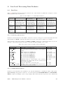
17
6
Getting started
This chapter describes how to set up the the environment and the analysis data and how to analyse data from
the two instruments that are part of IBIS: ISGRI and PICsIT. These two instruments are quite different in
energy range (ISGRI starts from 15 keV and PICsIT starts from 200 keV) and sensitivity, and are optimised
for different targets. This is why we have decided to guide you through the analysis of the crowded Galactic
Centre around 4U 1700-377 for ISGRI and of the bright Crab for PICsIT.
Here we assume that you have already successfully installed ISDC Off-line Scientific Analysis (OSA) Software
version 5.0 (the directory in which OSA is installed is later on referred to as the ISDC ENV directory). If
not, then look at the ”Installation Guide for the INTEGRAL Data Analysis System” [5], for detailed help.
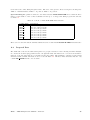
6.1
Setting up the analysis data
In order to set up a proper environment, you first have to create an analysis directory (e.g ibis data rep)
and ”cd” into it:
mkdir ibis_data_rep
cd ibis_data_rep
This working directory ibis data rep will be referred to as the “REP BASE PROD” directory in the
following. All the data required in your analysis should then be available from this “top” directory, and they
should be organized as follows
• scw/ : data produced by the instruments (e.g., event tables) cut and stored by ScWs;
• aux/ : auxiliary data provided by the ground segment (e.g., time correlations);
• cat/ : ISDC reference catalogue (OSA CAT package);
• ic/ : Instrument Characteristics (IC), such as calibration data and instrument responses (OSA IC
package);
• idx/ : set of indices used by the software to select approriate IC data (OSA IC package).
The cat/, ic/ and idx/ directories are part of the OSA software distribution and should be installed
following the “Installation Guide for the INTEGRAL Data Analysis System” [5]. The actual data along with
the auxiliary files (scw/ and aux/) are sent to the Principal Investigators of the observation. Alternatively,
the public data can be downloaded from the archive (see Section 6.1.1). In case the data are already available
on your system you can either copy these data to the relevant working directory, or better, create soft links
as shown below. Alternatively, if you do not have any of the above data on your local system, or if you do
not have a local archive with the scw/ and the aux/ branch available, follow the instructions in the next
section to download data from the ISDC WWW site.
ln
ln
ln
ln
ln
-s
-s
-s
-s
-s
directory_of_ic_files_installation__/ic ic
directory_of_ic_files_installation__/idx idx
directory_of_cat_installation__/cat cat
directory_of_local_archive__/scw scw
directory_of_local_archive__/aux aux
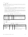
Then, just create a file ’isgri gc.lst’ containing the 5 lines:
scw/0051/005100410010.001/swg.fits[1]
scw/0051/005100420010.001/swg.fits[1]
ISDC – IBIS Analysis User Manual – Issue 5.1
18
scw/0051/005100430010.001/swg.fits[1]
scw/0051/005100440010.001/swg.fits[1]
scw/0051/005100450010.001/swg.fits[1]
and a file ’picsit.lst’ containing:
scw/0039/003900020020.001/swg.fits[1]
scw/0039/003900020030.001/swg.fits[1]
scw/0039/003900020040.001/swg.fits[1]
scw/0039/003900020050.001/swg.fits[1]
scw/0039/003900020060.001/swg.fits[1]
The created files contain the list of Scws you want to analyze (technically, we call them DOLs -Data Object
Locators-, i.e. a specified extension in a given FITS file 3 ).
These file names ‘isgri gc.lst’ and ‘picsit.lst’ will be used later as an argument for the og create program (see
Sections 7, 10).
6.1.1
Downloading data from the archive
• To retrieve the required ISGRI analysis data from the archive, go to the following URL:
http://isdc.unige.ch/index.cgi?Data+browse
You will reach the W3Browse web page which will allow you to build a list of Science Windows (SCWs)
that you will analyse with OSA.
- Type the name of the object (4U 1700-377) in the ‘Object Name Or Coordinates:’ field
- Do not forget to change ‘Search Radius’ if you are interested in science windows where your source
is in the partially coded field of view. Set it to e.g. 10 degrees
-Click on ‘More Options’ button at the top or at the bottom of the web page
- Deselect the ‘All’ checkbox at the top of the Catalog table, and select the ‘SCW - Science Window
Data’ one
- Press the ‘Specify Additional Parameters’ button at the bottom of the web page
Introduce values in the fields of interest. For instance:
- Sort output by scw id, for that check the ‘Sort’ column.
- Put pointing in the field ‘scw type’ (to specify that only pointings should be returned and not e.
g. slews)
- Put >=2003-03-15 23:00:00 in the field ‘start date’ and put <= 2003-03-16 02:30:00 in the
field ‘end date’
- Put public in the field ‘ps’ (to specify that only public ScWs should be returned)
- Put > 100 in the field ‘good isgri’ (to select Science Windows with good ISGRI time higher than
100 seconds)
- Press the ‘Start Search’ button at the bottom of the web page. In our case, a table with 5 ScWs will
be displayed.
- Select the SCWs of interest. To follow the example in the Cookbook click on All (for all SCWs).
- Press the ‘Save SCW list for the creation of Observation Groups’ button at the bottom of that
table and save the file with the name ‘isgri gc.lst’. This file ‘isgri gc.lst’ will be used later as input for
the og create program (see Section 7). From this file you need the 5 lines:
scw/0051/005100410010.001/swg.fits[1]
scw/0051/005100420010.001/swg.fits[1]
3 When an analysis script asks you to specify the DOL, you should specify the path of the corresponding FITS file, and the
corresponding name or number of the data structure in square brackets(do not forget that numbering starts with 0!). See more
details in the Introduction to the INTEGRAL Data Analysis [1]. Please note that the naming scheme is different for revision
1 and revision 2 data. For the revision 1 data, the name of the prepared Science Window Group is swg prp.fits instead of
swg.fits.
ISDC – IBIS Analysis User Manual – Issue 5.1
19
scw/0051/005100430010.001/swg.fits[1]
scw/0051/005100440010.001/swg.fits[1]
scw/0051/005100450010.001/swg.fits[1]
You should then download them pressing the ’Request data products for selected rows’ button. In the
‘Public Data Distribution Form’, provide your e-mail address and press the ‘Submit Request’ button.
You will be e-mailed the required script to get your data and the instructions for the settings of the
IC files and the reference catalogue. Just follow these instructions.
• To retrieve the required PICsIT analysis data from the archive proceed in the same manner with the
following parameters:
- ‘Object Name Or Coordinates:’ Crab
- ‘Search Radius’ : default value
- ‘scw id’ : 0039% (To select only science windows starting with 0039)
- ‘start date’ : >=2003-02-07 06:44:19 and ‘end date’: <=2003-02-07 12:44:05
and save your results in a file called ‘picsit.lst’ which should contain:
scw/0039/003900020020.001/swg.fits[1]
scw/0039/003900020030.001/swg.fits[1]
scw/0039/003900020040.001/swg.fits[1]
scw/0039/003900020050.001/swg.fits[1]
scw/0039/003900020060.001/swg.fits[1]
6.2
Setting the environment
Before you run any OSA software, you must also set your environment correctly.
The commands below apply to the csh family of shells (i.e csh and tcsh) and should be adapted for other
families of shells4 .
In all cases, you have to set the REP BASE PROD variable to the location where you perform your analysis (e.g
the directory ibis data rep). Thus, type:
setenv REP_BASE_PROD
$PWD
Then, if not already set by default by your system administrator, you should set some environment variables:
setenv ISDC_ENV directory_of_OSA_sw_installation
setenv ISDC_REF_CAT "$REP_BASE_PROD/cat/hec/gnrl_refr_cat_0023.fits[1]"
source $ISDC_ENV/bin/isdc_init_env.csh
The latter command executes the OSA set-up script (isdc init env.csh) which initialises further environment variables relative to ISDC ENV. Ignore all warnings mentioning ROOTSYS.
Besides these mandatory settings, the optional environment variable COMMONLOGFILE can also be useful.
By default, the software logs messages to the screen (STDOUT). To have these messages in a file (i.e
common log.txt), and make the output chattier5 use the command:
setenv
COMMONLOGFILE +common_log.txt
4 If
the setenv command fails with a message like:‘setenv: command not found’ or ‘setenv: not found’, then you are probably
using the sh family. In that case, please replace the command ‘setenv my variable my value’ by the following command sequence
‘my variable=my value ; export my variable’
In the same manner, replace the command ‘source a given script.csh’ by the following command ‘. a given script.sh’ (the ‘.’ is
not a typo!).
5 For
example, the exit status of the program will now appear.
ISDC – IBIS Analysis User Manual – Issue 5.1
20
6.3
6.3.1
Two ways of launching the analysis
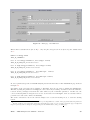
Graphical User Interface (GUI)
When you launch the analysis the Graphical User Interface (GUI) is launched, providing an opportunity to
set the values of all desired parameters, see Figure 12. On the right side of the panel you see the following
buttons:
• Save as – With the ”Save As” - button a file is created. This file stores all parameters as they are
currently defined in the GUI as a command line script. This file is an executable one and calling it
from the command line will launch the instrument analysis program with the parameters as they were
defined in the GUI.
• Load With the ”Load” - button a previously saved file (see ”Save As”) can be read and the GUI will
update all parameters with the values as they are defined in the loaded file.
• ResetWith the ”Reset” - button the parameters in the GUI will be reset to the default values as they are
defined in the parameter file of the instrument analysis program and stored in the $ISDC ENV/pfiles
directory.
• Run With ”Run” - button the analysis is launched.
• Quit With ”Quit” - button you quit the program without analysis launch.
• Help With ”Help” - button the help file of the main script is opened in a separate window.
• hidden With the ”hidden” - button you have an access to the hidden parameters with values defined
by the instrumental teams. Change them with care!
6.3.2
Launching scripts without GUI
Alternatively, parameters can be specified on the command line typing ’name = value’ after the script
name.
If you are running your own scripts that call OSA many times you don’t want GUI to pop up each time. In
such a case set COMMONSCRIPT variable to “1” with:
setenv COMMONSCRIPT 1
This is automatically done within the file created with the help of ”Save as” - button, see above.
To have the GUI back again, unset the variable:
unsetenv COMMONSCRIPT
6.4
Useful to know!
• How do I get some help with the executables?
All the available help files are stored under $ISDC ENV/help. To visualize a help file interactively
type tool name --h once your environment is set (i.e. which tool name returns the path to it).
• Where are the parameter files and how can I modify them?
All the available executables for the analysis of INTEGRAL data are under $ISDC ENV/bin. The
corresponding parameter files are stored under $ISDC ENV/pfiles/*.par. The first time you launch
a script, the system will copy the specific tool.par from $ISDC ENV/pfiles/ to a local directory
(/user name/pfiles/). The parameter file in the local directory is the one used for the analysis and is
ISDC – IBIS Analysis User Manual – Issue 5.1
21
the one you can modify. If this parameter file is missing (e.g. you have deleted it), the system will
just re-copy it from $ISDC ENV/pfiles/ as soon as you launch the script again. The system knows
what to copy from where thanks to the $PFILES environment variable that is also used in FTOOLS
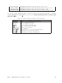
(http://heasarc.gsfc.nasa.gov/ftools/). Each parameter is characterized with a letter that specifies the
parameter type, i.e:
”q” (query) parameters are always asked to the user
”h” (hidden) parameters are not asked to the user and the indicated value is used
”l” (learned) parameters are updated with the user’s value during the use of the program.
The GUI is a fast and easy way to change the parameters, see section 6.3.1 for details.
• What are groups and indices?
The ISDC software makes extensive use of groups and indices. While it is not necessary to grasp all
the details of these concepts, a basic understanding is certainly quite useful.
As implied by their names, ”groups” make possible the grouping of data that are logically connected.
Groups can be seen as a kind of data container, not completely unlike standard directories. At ISDC,
we create separate groups for each pointing, in which we store the many different data types produced
by Integral and its instruments. The user then only has to care about one file, the group, many tens
of files being silently included. Several pointings (the ”Science Window Groups”) can be arbitrarily
grouped into bigger groups (the ”Observation Group”) to select data very efficiently according to the
user’s needs.
Indices are a special kind of groups, which differ only in the fact that all the the data sets they contain
are similar and that the indices know the properties of the data sets they contain. Indices are a kind of
poor man’s database. For example, an imaging program creates several images of different types (flux
map, significance map,...) in different energy bands. These images are stored in an index, in which
the image type and energy band information is replicated. ISDC software is then able to select very
efficiently the needed images. The user can also make use of the indices; just by looking at the index
(for instance using ”fv”), the user can identify immediately the content of each image.
• Why do I need ”[1]” after a FITS file name?
A FITS file can have many extensions and sometimes it is necessary to specify as input to a given parameter not the file name alone (file.fits) but the extension too (file.fits[1], or file.fits[2],
etc). The file name with a specified data structure (extension) is called DOL (Data Object Locator). When you modify the parameter file itself (see above) or use the GUI, the extension will be
correctly interpreted in the file.fits[1] case. On the command line though, the normal CFITSIO
and FTOOLS rules apply, i.e. you have to specify it as one of the following
file.fits\[1]
file.fits+1
"file.fits[1]".
Note that if no extension is specified explicitly then the first one ([1]) will be used by default.
ISDC – IBIS Analysis User Manual – Issue 5.1
22
7
A Walk through ISGRI Analysis
After setting up as described in the previous section, you are ready to analyse the data.
Please do remember that you are dealing with a coded mask instrument not with a focussing
telescope and a CCD. It is not possible to deal with one source at a time: each source is
background for the others, the whole field of view - and not just the few pixels around your
source - matters!
In this Section, we guide you through your first IBIS analysis, but please read also Section 8,
where more details on the main parameters are given. You could end up with fake sources
that are created by a blind use of parameters! More tips and tricks are given in Section 9 for
advanced users.
In the example below we analyze observations of the Galactic Center, using data we have downloaded and
installed as it is described in Section 6.1.
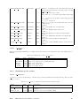
Create the Observation Group with the og create program (see its description in the Toolbox section of [1]):
cd $REP BASE PROD
og_create idxSwg=isgri_gc.lst ogid=isgri_gc
baseDir="./" instrument=IBIS
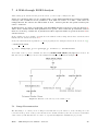
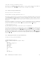
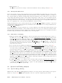
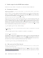
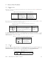
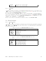
As a result of the og create command, the directory $REP BASE PROD/obs/isgri gc is created. In
this directory you find all you need for the analysis, its structure is illustrated in Figure 11.
Figure 11: Structure of the directory created with og create
7.1
Image Reconstruction
The first thing to do when you are looking for the first time at your data is to create an image in order
to know how the portion of sky you are interested in looks like, whether your source is detected, and what
other sources you should take into account to do spectral and lightcurve analysis in a proper way.
ISDC – IBIS Analysis User Manual – Issue 5.1
23
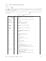
To start the analysis, move to the working directory $REP BASE PROD/obs/isgri gc and call the
ibis science analysis script:
cd obs/isgri_gc
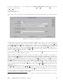
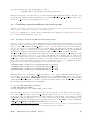
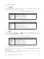
ibis_science_analysis
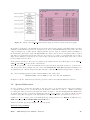
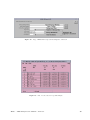
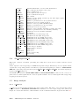
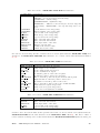
After a few seconds the main page of the IBIS Graphical User Interface (GUI) appears, as shown in Figure
12.
Figure 12: Main page of the IBIS GUI
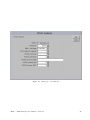
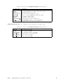
Keeping all the default values, you will make an analysis starting from the energy correction level (startLevel
= COR) until the image reconstruction level (endLevel = IMA2 6 ). The default input catalog (CAT refCat
= $ISDC REF CAT[ISGRI FLAG==1]) will be used: it contains the sources that were detected by ISGRI
in the public data up to April 2005. ISGRI data alone will be processed (SWITCH disablePICsIT=yes)
through all the available levels shown in GENERAL levelList within COR and IMA2. No additional good
time interval will be applied to the data: SCW1 GTI gtiUserI field is empty, which also implies that the last
parameter SCW1 GTI TimeFormat is not effective.
You are ready to set the parameters specific for imaging. Press the ISGRI IMA button at the bottom of the
GUI. Another box, shown in Figure 13 appears.
With the parameters displayed in the GUI, you will create 4 different images of the sky, corresponding to 4
energy bands (IBIS II ChanNum=4) in the ranges 20–40, 40–60, 60-100 and 100-200 keV. You will let the
software look for the 15 brightest sources in the field of view (OBS1 Searchmode=2 and OBS1 ToSearch=15),
with detection significance higher than 6 for catalog sources (OBS1 MinCatSouSnr=6), and 7 for new sources
(OBS1 MinNewSouSnr=7). Given that you are analysing the crowded Galactic center, it might be better to
increase the number of sources you are looking for. Change manually OBS1 ToSearch to 25. The position of
all the catalog sources will be fitted (OBS1 SouFit=0). Resulting images will be cleaned with the available
background maps provided by the IBIS team (empty value of SCW1 BKG I isgrBkgDol means usage of the
default map
$REP BASE PROD/ic/ibis/bkg/isgr back bkg 0005.fits). After creation of all the individual science window
images the mosaic image will be created (OBS1 DoPart2=1). In this mosaic image the photons belonging to
a source are spread around the single central peak (OBS1 PixSpread=1), resulting in better source location.
Now that you have checked all the parameters, press Ok, the Imaging window disappears and you are back
to the main GUI page. Press Save, and then Run.
6 IMA2 level is for PICsIT analysis only, and there is no difference for ISGRI analysis whether endLevel is set to IMA, or
IMA2.
ISDC – IBIS Analysis User Manual – Issue 5.1
24
Figure 13: Imaging page of IBIS GUI
7.1.1
Results from the Image Step
When the analysis is finished, you will find that new files have appeared in your working directory. In
Figure 14 an overview of the files related to the image reconstruction is given. The full description of all
files produced at different levels is given in Appendix C.
As it is shown in Figure 14, there are results for each science window as well as for the overall group.
Science window results include:
• Images: scw/0051004X0010.001/isgri sky ima.fits (X=1..5)
for each energy range four images are produced: intensity, variance, significance7 and residual8 . To
know which type of image and which energy band correspond to a given extension, you can either
check in the header of the isgri sky ima.fits files, or check the first extension of the file – an index,
summarizing the file content, see Figure 15. More details on index concept are in [1].
• Detected source list: scw/0051004X0010.001/isgr sky. res.fits (X=1..5)
list of the sources detected in each energy range with reconstructed RA, DEC, flux, error and significance.
Observation group results include:
• Images: isgri mosa ima.fits
The structure of this file with the mosaic images is similar to the one of isgri sky. ima.fits, but instead
of residual maps you have the exposure ones.
• Detected source list: isgri mosa res.fits
list of the sources detected in the mosaic image in each energy range with reconstructed RA, DEC,
flux, error and significance.
The single science window and mosaic results are merged in the file isgri srcl res.fits. This file contains all
the sources from the isgri catalog.fits plus all the new sources, with the information on their fitted position,
fluxes, and detection level.
7 Note
8 The
that systematic errors are not included in the calculation of the detection significance (DETSIG).
intensity image from which all photons attributed to the detected sources were removed
ISDC – IBIS Analysis User Manual – Issue 5.1
25
Figure 14: Overview of the IMA level products
You find more details on the structure of the output files in Section C.7.1.
7.1.2
Displaying the Results from the Image Step
It is convenient to look at the images with the help of the ds9 program. First create a region file from the
catalog using the cat2ds9 program. In the example below we create the region file found.reg with all the
sources found in the mosaic image, isgri mosa res.fits, for the first energy band (extension number 2), and
a region file cat.reg with all sources that were in the input catalog isgri catalog.fits.
cd $REP_BASE_PROD/obs/isgri_gc
cat2ds9 isgri_mosa_res.fits\[2] found.reg symbol=box color=green
cat2ds9 isgri_catalog.fits\[1] cat.reg symbol=box color=white
To see the resulting images:
ds9 $REP_BASE_PROD/obs/isgri_gc/isgri_mosa_ima.fits\[2] \
-region $REP_BASE_PROD/obs/isgri_gc/cat.reg\
-cmap b -scale sqrt -scale limits 0 60 -zoom 2\
$REP_BASE_PROD/obs/isgri_gc/isgri_mosa_ima.fits\[4]\
-region $REP_BASE_PROD/obs/isgri_gc/found.reg\
-cmap b -scale sqrt -scale limits 0 60 -zoom 2
In Figure 16 you see the intensity $REP BASE PROD/obs/isgri gc/isgri mosa ima.fits[2] (left) and significance $REP BASE PROD/obs/isgri gc/isgri mosa ima.fits[4] (right) mosaic images in the 20 – 40 keV
energy range. In the left image we have shown all catalog sources (white boxes), and in the right one only
the detected ones (green boxes). As you can see, there are three sources labelled as NEW. This example
ISDC – IBIS Analysis User Manual – Issue 5.1
26
Figure 15: Sketch of the isgri sky ima.fits structure (left), and extract from the Index table (right).
shows that you should be careful with the new sources found by the software, and always make a detailed
analysis to verify whether they are real or spurious ones. In a coded mask instrument a true point source will
cause secondary lobes, 8 main ”ghosts” aligned with the detector edges, at a distance that is a multiple of
the mask basic pattern, 10.7 degrees in IBIS/ISGRI case. If the source is detected, its ghosts will be cleaned
and will not be included in the mosaic. However, if a source is too weak to be automatically detected in a
single Science Window, its ghosts are not cleaned, they can appear in the mosaic image and even be found
by the software as new sources.
In the present case, three sources were recognized by the software as new ones. These three sources, NEW 1,
NEW 2, and NEW 3, are the ghosts of 4U 1722-30.
There is an easy way to collect from different science windows all the information related to a given source
and energy band. In the example below we create a file 4U1700-377 scwlc.fits with all the information on
4U 1700-377 in 20 – 40 keV energy band. The structure of this file is explained in Appendix C.7, Table 53.
src_collect group=og_ibis.fits+1 results=4U1700-377_scwlc.fits
instName=ISGRI select="NAME == ’4U 1700-377’ && E_MIN==20"
In Figure 17 the 20 – 40 keV science window per science window 4U 1700-377 lightcurve is shown.
7.2
Spectral Extraction
It is not possible to extract the spectrum of only the source you are interested in. All sources brighter
or compatible with the one you are interested in should be taken into account too. Thus it is strongly
recommended, when you deal for the first time with your data, to run the analysis until the IMA2 level,
as described in Section 7.1, check the results, and call ibis science analysis once again to run the spectral
extraction part. The description of the algorithm used for spectral extraction is given is Section 12.9.1.
Launch ibis science analysis, and on the main GUI page change Start Level to BIN S, and End Level to
SPE. After that press the ISGRI SPE and LCR button.
On the screen that appears (see Figure 18), you can specify:
Spectral energy binning:
ISDC – IBIS Analysis User Manual – Issue 5.1
27
Figure 16: Intensity (left) and significance (right) mosaic in the 20 – 40 keV energy band
With the help of the parameter IBIS SI inEnergyValues you can specify the file (and its extension) describing the desired binning of the response matrix. By default (set with empty line), the latest available
file with the rebinned response matrix is used. Currently it is
$REP BASE PROD/ic/ibis/rsp/isgr rmf grp 0017.fits[3] with 16 channels in it.
See sections 8.3 and 9.4 if you want to define your own spectral binning.
Background maps:
With the SCW2 BKG I isgrBkgDol parameter you can specify the background map to be used in the
spectral and timing analysis. It is recommended to use the same background map as in the imaging case. Default empty value corresponds to the default map ($REP BASE PROD/ic/ibis/bkg/isgr back bkg 0005.fits).
Input catalog for Spectral and Lightcurve extraction:
By default a spectrum will be created for all sources listed in the isgri srcl res.fits catalog created
during the IMA step. The position of the source will be taken from RA FIN, DEC FIN columns. Note
however that spectral extraction is time consuming, and it is not recommended to include sources that are
faint in comparison with the source of interest. It is not recommended to have more than 30 sources
in the input catalog, as the software might crash otherwise. Copy isgri srcl res.fits to another file,
say specat.fits as shown below, leaving only sources with significance higher than 6:
cd $REP_BASE_PROD/obs/isgri_gc
fcopy "isgri_srcl_res.fits[ISGR-SRCL-RES][DETSIG >= 6.0]" specat.fits
(Note, that there should be spaces around ”>=”).
As we have discussed in Section 7.1.2, all found new sources are fake ones, so remove them with the help of
the fv command, and make the resulting catalog read only (this is important because the file could otherwise
get corrupted during the analysis):
chmod -w
specat.fits
The resulting specat.fits catalog is shown in Figure 19 (only a few selected columns are shown). The same
ISDC – IBIS Analysis User Manual – Issue 5.1
28
Figure 17: 4U 1700-377 science window per science window lightcurve in the 20 – 40 keV energy band
ISDC – IBIS Analysis User Manual – Issue 5.1
29
Figure 18: Page of IBIS GUI for Spectral and Ligtcurve extraction
Figure 19: List of sources used for spectral analysis
ISDC – IBIS Analysis User Manual – Issue 5.1
30
catalog will be used later for the lightcurve extraction.
In the GUI, set the SCW2 cat for extract parameter to point to specat.fits[1] and press Ok, the
window disappears and you are back to the main GUI page. Press Save, and then Run.
7.2.1
Results of the Spectral Extraction
Spectra are produced for each science window:
scw/0051004X0010.001/isgri_spectrum.fits (X=1..5)
In these files you find the spectra of the desired sources plus the background spectrum. In the header
of each data structure, the Name and ID of each source are given, and the first extension of the file
scw/0051004X0010.001/isgri spectrum.fits[1] is an index, summarising the content of all the extensions.
With the help of this index you can easily see which extension contains the spectrum of the source you are
interested in.
To achieve a better signal to noise ratio, it can be convenient to sum up spectra of a source from different
science windows. This can be done with the spe pick tool. In the following example we create a joint
spectrum of 4U 1700-377 from all the available science windows (included in the og ibis.fits file).
cd $REP_BASE_PROD/obs/isgri_gc
spe_pick group="og_ibis.fits[1]" source="4U 1700-377" rootname=4U1700
As a result two files with spectra of 4U 1700-377 will be created: 4U1700 sum pha.fits contains the final
average spectrum of 4U 1700-377, while 4U1700 single pha2.fits stores all the original spectra of 4U 1700-377
that were used to create the average one. It is forseen that in the nearest future there will be several ARFs,
depending on the data time. In order to deal with the data from different time periods spe pick was updated
and creates now a resulting ARF for your particular dataset. This ARF is written to 4U1700 sum arf.fits
and 4U1700 single arf.fits files. At the moment only one ARF is present and is copied as it is to the files
mentioned above.
7.2.2
Displaying the Results of the Spectral Extraction
To analyze the average spectrum with XSPEC do
cd $REP_BASE_PROD/obs/isgri_gc
fparkey 0.02 4U1700_sum_pha.fits SYS_ERR
xspec
cpd /xw
data 4U1700_sum_pha.fits
setpl energy
ign **-22.5
ign 150.-**
plot ldata
model cutoffpl
1.7
33
3
fit 100
plot ldata del
add=yes
ISDC – IBIS Analysis User Manual – Issue 5.1
31
The resulted 4U 1700-377 total spectrum is shown in Figure 20. Please note that in OSA 5.0 reconstructed
ISGRI spectra are not accurate below 17 keV. ISGRI systematic is believed to be equal to 1%.
In the very same manner, you can sum up the spectra for all the sources of the input catalog, specified in
the SCW2 cat for extract parameter9 .
Figure 20: Total 4U 1700-377 spectrum.
Usage of spe pick for spectra created in different observation groups is explained in Section 9.
7.3
Lightcurve Extraction
After you have done the spectral extraction, you may want to produce a lightcurve for the same sources.
Stay in the working directory $REP BASE PROD/obs/isgri gc and call the ibis science analysis script
again. On the main GUI window (see Figure 12), change both Start Level and End Level to LCR, and press
the ISGRI SPE and LCR button. The GUI shown in Figure 18 will appear.
Note that to extract the lightcurve for a source you need the Pixel Illuminated Fraction (PIF10 ) map.
Such a map is created during the spectral step that we have just run. This means that at this stage you
can extract the lightcurve only of the sources for which a spectrum has been created already. So leave
SCW2 cat for extract to point to specat.fits.
By default, for each source from the input catalog (specat.fits in our example), four lightcurves (in 20 –
40, 40 – 60, 60 – 100, and 100 – 200 keV energy bands) with 100 sec time bins will be created.
The lightcurve extraction is performed by building shadowgrams for each time and energy bin. Hence this
step is time and space consuming. Note that due to CFITSIO limitations, the product of number of
energy bins by number of time bins in a science window should be less than 250.
Press Ok, the window will disappear and you are back to the main GUI page. Press Save, and then Run.
9 To
read a given extension in XSPEC you have to specify it in curly brackets: ”data pha.fits{3}”
is a number between 0 and 1, which expresses the theoretical degree of illumination of each detector pixel for a given
source in the sky.
10 PIF
ISDC – IBIS Analysis User Manual – Issue 5.1
32
7.3.1
Results of the Lightcurve Extraction
Lightcurves are produced for each science window:
scw/0051004X0010.001/isgri_lcr.fits (X=1..5)
To create a merged lightcurve in the 20 – 40 keV energy range (i.e. to store in one file all the available
lightcurves of a given source) use lc pick :
lc_pick source=’4U 1700-377’ attach=n \
group=og_ibis.fits+1 lc=4U1700-377.fits emin="20" lcselect=’E_MAX==40’
The result is written to 4U1700-377.fits. It is possible to create more than one merged lightcurve at a
time if you specify a list of desired minimum energies with the parameter emin. If you have more than
one energy range with the same minimal energy, then you should use the parameter lcselect to define the
unique energy band, otherwise the lcselect parameter can be omitted.
7.3.2
Displaying the Results of the Lightcurve Extraction
To see the source lightcurve, you should plot the column RATE with error ERROR versus column TIME,
whereas to see the background lightcurve, you should plot column BACKV with error BACKE versus column
TIME.
To display the resulting lightcurve it is convenient to use the lcurve program from the FTOOLS package:
lcurve
Number of time series for this task[] 1
Ser. 1 filename +options (or @file of filenames +options)[] 4U1700-377.fits[2]
Name of the window file (’-’ for default window)[] Newbin Time or negative rebinning[] 100
Number of Newbins/Interval[] 95
(take this number from the line above:
Maximum Newbin No. 95)
Name of output file[default]
Do you want to plot your results?[] yes
Enter PGPLOT device[] /XW
hardcopy 4U1700-377_lc.ps/PS
quit
As a result, the 4U1700-377 lc.ps file was produced and is shown in Figure 21.
ISDC – IBIS Analysis User Manual – Issue 5.1
33
Figure 21: 4U1700-377.fits lightcurve in 20 – 40 keV energy range with 100 sec binning.
8
More on ISGRI relevant parameters
In the first part of the Cookbook (Section 7), the default values of the parameters were used. Now, it is time
to discuss in more details the usage of the main parameters. The full list of parameters along with short
explanations is given in Table 61, Appendix D.
8.1
How to choose the start and end level for the analysis
When you launch an analysis you have to decide which levels to perform (see Section 5 for a description of
the different levels). This choice is done with the parameters startLevel and endLevel. We recommend to
use startLevel="COR" in any case, even if you are using revision 2 data: in OSA 5, you have more accurate
energy correction than was available at the time of the revision 2 data archiving. Therefore, it is worth
redoing this step.
Once you have specified startLevel and endLevel, all the steps listed in the GENERAL levelList parameters
between these two levels (both included) will be performed. For instance, in section 7.1 you used:
startLevel="COR" endLevel="IMA2"
GENERAL_levelList="COR,GTI,DEAD,BIN_I,BKG_I,CAT_I,IMA,IMA2,BIN_S,SPE,LCR,COMP,CLEAN"
The levels from COR to IMA2 (included) listed in GENERAL levelList were performed.
You can choose what to run according to what kind of output you need. Basically:
• If you are interested only in imaging results set
startLevel="COR" endLevel="IMA2"
with the complete list of GENERAL levelList given above, as done in section 7.1.
• If you have already a catalog of sources for which to extract the spectra (e.g.specat.fits11 ) and you
are not interested in the imaging results anymore you can skip all the imaging related levels and do:
11 specat.fits has to be of the ISGR-SRCL-RES type, meaning that it has to be created by the imaging step (with
OBS1 DoPart2=1, since this file is created at mosaic stage). See section 7.2 to learn how to go from the imaging result
file isgri srcl res.fits to your specat.fits, to avoid software crash.
ISDC – IBIS Analysis User Manual – Issue 5.1
34
startLevel="COR" endLevel="SPE" GENERAL_levelList="COR,GTI,DEAD,BIN_S,SPE"
Remember that if you do not do the imaging part then isgri srcl res.fits is not created! This file
is the default one that is used for spectral extraction (7.2). Do not forget to specify the catalog you
have built for this purpose setting the SCW2 cat for extract equal to specat.fits[1].
• Likewise, if you are interested only in lightcurve results you should create PIFs for all source of interest
with ii pif program (see Section 9.10 for an example), and afterwards you may use:
startLevel="COR" endLevel="LCR" GENERAL_levelList="COR,GTI,DEAD,BIN_S,LCR"
again with SCW2 cat for extract equal to specat.fits[1].
• If you are familiar with the sources of your field (i.e. you have already run the imaging part, for instance)
and you want to extract images, spectra and lighturves in one go, set SCW2 cat for extract equal to
specat.fits[1] and run your analysis with
startLevel="COR" endLevel="LCR"
and the complete list of levels in GENERAL levelList.
8.2
Imaging
Source detection is an important and delicate process as the background and all the sources (especially
the bright ones) in the field of view will have an impact on it. Because of this intrinsic complexity of the
instrument, there are different options as far as source search and background correction are concerned. The
choice of the best method to use for a given case may require a bit of iteration on your side.
In the next two paragraphs we describe the parameters involved in the source search, along with some
practical advices. The single Science Window case is treated in Section 8.2.1, while the mosaic image case
in Section 8.2.2. Comments on the background subtraction issue are given in Section 8.2.3 while a set of
miscellanea on imaging parameters is given in Section 8.2.4.
8.2.1
How to choose the source search method in the Science Window analysis
Basically the idea is that you can either let the software look for the excesses in the field or you can tell
the software to look for sources from a given catalog. This catalog can be either the one provided by ISDC
(CAT refCat="$ISDC REF CAT"), from which you can extract e.g. only the sources that have been detected
by ISGRI (”$ISDC REF CAT[ISGRI FLAG==1]”), or a catalog made on your own (see section 9.6 to create a
catalog on your own). The number of sources that are detected in an image is important because detecting
a source means also removing its ghosts from the images 12 (see section 7.1).
The source search method is defined with the parameters OBS1 SearchMode and OBS1 ToSearch. These
parameters allow you the following possibilities:
• OBS1 SearchMode = 0
This mode was developed for testing purposes and is not recommended for scientific use.
• OBS1 SearchMode = 1
the software will look for all the sources of the input catalog that are in the field of view (regardless
of their detection level). If the source gives a positive detection, then the relevant results are saved in
the isgri sky res.fits file, but see also discussion on OBS1 NegModels in Section 8.2.4.
This mode can be useful in case your Science Window images are noisy and many fake new sources
are detected. Searching only the sources from a given catalog will avoid having ghost cleaning for fake
sources.
12 Note
that the run time is proportional to the number of sources detected.
ISDC – IBIS Analysis User Manual – Issue 5.1
35
• OBS1 SearchMode = 2
The software will look for the K brightest sources in the field, where K = OBS1 ToSearch.
They can be either known sources (more significant than OBS1 MinCatSouSnr) or new sources (more
significant than OBS1 MinNewSouSnr).
This mode is useful if you are interested in having a first glance at your field, if you are interested in
bright sources only, or if you run your analysis on large data sets. In fact, in these cases you would not
like to spend most of your time collecting information on weak sources that are not detected in a single
Science Window. The drawback of this method is that these undetected weak sources can produce
ghosts in the mosaic image. We recommend you to start the analysis with OBS1 SearchMode = 2 with
a high OBS1 ToSearch value (around 20, especially for the Galactic plane or Centre crowded regions),
see the sources that are detected and prepare your own catalog of detected sources (see section 9.6).
Then launch again the analysis with OBS1 SearchMode = 3 - described below - and give your catalog
as input for the analysis (CAT refCat=‘‘usrcat.fits[1]’’).
• OBS1 SearchMode = 3
The software will look for all the catalog sources (regardless of their detection level) plus for K significant
excesses more significant than OBS1 MinNewSouSnr, where K = OBS1 ToSearch. All these sources will
be saved in the final isgri sky res.fits file if their detection significance is positive, but see also
discussion on OBS1 NegModels in Section 8.2.4 . This mode is very efficient in cleaning the ghosts of
all the sources in the field of view. It is of course more time consuming since a model is created and
deconvolved for each given source.
We suggest that you should use this mode either with your own catalog (built from the previous run
with
OBS1 SearchMode = 2, see above) or, if no personalised catalog is available, using the ISDC catalog
with only the sources that have been detected by ISGRI ($ISDC REF CAT[ISGRI FLAG==1], see above).
Any bright source out of the catalog (new or forgotten!) will be detected as one of the K new sources.
8.2.2
Parameters related to the mosaic step
The OBS1 SearchMode parameter concerns only images at a Science Window level. In the mosaic image the
software always looks for K=OBS1 ToSearch sources (more significant than OBS1 MinCatSouSnr for catalog
sources, or OBS1 MinNewSouSnr for the new sources), regardless the real number of sources in the field of
view. Thus, if you are working with a crowded part of the sky (mainly Galactic plane and Centre) you
should use a high OBS1 ToSearch number (at least 20).
There are two ways to calculate the source flux in the mosaic given the original Science Window information:
• OBS1 PixSpread = 0
The whole input (Science Window) pixel count is put into one output (mosaic) pixel, no ”spread” is
done. This method optimises the flux and signal-to-noise ratio (SNR) evaluation but can sometimes
give some undesired effects such as double source peaks.
• OBS1 PixSpread = 1 (default value)
The input pixel count is spread between different output map pixels. This method is better for the
source position estimate but is less accurate than the previous method for source flux estimation. SNR
in the new spread mosaic will be lower than in the previous case.
It is possible to decide whether you want the mosaic to be created along with the Science Window image
reconstruction, or if you prefer it to be created later on. The mosaic production is controlled by the
OBS1 DoPart2 parameter:
• OBS1 DoPart2 = 0
The mosaic step is not performed and the imaging part ends after the Science Window based part.
• OBS1 DoPart2 = 1 (default value)
The mosaic is done after the Science Window image reconstruction, in the same run.
ISDC – IBIS Analysis User Manual – Issue 5.1
36
• OBS1 DoPart2 = 2
The mosaic is performed for images obtained from different, already existing, runs (see 9.3.1).
8.2.3
Background Subtraction
In the current OSA you have background maps provided by the ISGRI team. These maps are created on the
base of observations containing only faint sources in their fields of view. Currently, a single set of maps for
the complete mission is available, meaning that background variations are not taken into account. In most
cases background subtraction improves the result, nevertheless we cannot state a priori in which cases the
background subtraction will improve (or worsen) the results. The best approach is to verify in the images if
the background subtraction is working correctly (giving a better image) before deciding what results to use
and before applying it also to the spectral and lightcurve extraction levels.
Background subtraction can be tuned with the help of the SCW1 BKG I isgrBkgDol parameter. If it is left
empty then the background map is taken automatically from the IC files. To have no background subtraction,
set SCW1 BKG I isgrBkgDol=‘‘-’’.
As a general guideline, for short timescale (e.g. 1 Science Window), the background features should be less
than the statistical uncertainties so that background removal is not expected to change the result by much.
On longer time scales (mosaic image), things can be different, especially in the case of a Staring observation
in which background features can accumulate and become important.
8.2.4
Miscellanea on Imaging
• With the parameter OBS1 ExtenType (to find it on the GUI pages press the hidden button, and go to
the IMA page) you can choose whether to keep the Residual and/or the true Exposure image in the
isgri sky ima.fits file. With the default, “0”, 4 maps will be created per energy range (Intensity,
Variance, Significance and Residuals). With OBS1 ExtenType = 1 true exposure maps will be written
instead of residual images at the 4*n extension of isgri sky ima.fits. OBS1 ExtenType = 2 will add the
true Exposure maps in an additional extension. OBS1 ExtenType = 3 will add single true Exposure
map as the last extension.
• If you are interested in running the analysis in more than 10 energy bands please see Section 9.4.
• You can decide if you want to let the software find the best fit position of a source (in the vicinity of the
one in the catalog, default OBS1 SouFit=0), or if you would prefer the catalog position (for all sources
from the input catalog!) to be used for the flux determination (OBS1 SouFit=1). If OBS1 SouFit=1,
then the position of a new source is always attributed to the pixel center, and for catalog sources
the catalog position is used for SearchMode=1,3, or the pixel center for SearchMode=2. Note that
OBS1 SouFit=1 fixes all the source positions only in the individual Science Window analysis. In the
mosaic, all source positions are always fitted regardless of the value of OBS1 SouFit. This fitted values
are written to RA FIN and DEC FIN columns of isgri-srcl-res.fits, and are later used in spectral and
lightcurve extraction steps as a source position. To fix the positions of only several sources, set for
them ISGRI FLAG=2 in the input catalog.
• For OBS1 SearchMode = 1 or 3 (where you are forcing a catalog extraction) ghosts can be cleaned even
from the known sources that happen to have a negative peak. This is done using OBS1 NegModels
= 1 while with OBS1 NegModels empty or equal to “0” (the default) the deconvolved images will be
cleaned from positive source ghosts only.
8.3
8.3.1
Spectral and Timing Analysis
Spectral Energy Binning
With the help of the IBIS SI inEnergyValues parameter you can specify the desired binning of the response
matrix. See Section 9.4 for the detailed discussion on how to rebin the original response matrix.
ISDC – IBIS Analysis User Manual – Issue 5.1
37
In case you using a response matrix rebinned on your own you should set
SCW2 ISPE idx isgrResp=”your rebinned matrix.fits”. Warning:This parameter is a hidden one in OSA
5.1. Thus you should either provide the value of this parameter during the script launch
ibis_science_analysis SCW2_ISPE_idx_isgrResp="your_rebinned_matrix.fits"
or press ”hidden”-button and set this parameter on the SPE page.
8.3.2
Background Subtraction
In spectral and timing analysis you can choose (with the help of the parameter SCW2 BKG I isgrBkgDol)
whether you want to subtract the instrumental background or not, similarly to the imaging case. We
recommend you to use the option that gives the best results at the imaging level (smoother image, no clear
patterns etc). See 8.2.3 for more information.
8.3.3
Input catalog
The single Science Window and mosaic imaging results are merged in the file isgri srcl res.fits. By
default a spectrum and a lightcurve will be created for all sources listed in this file. Spectral/lightcurve
extraction is time consuming and we recommend you to create an input catalog for spectral and timing
extraction, as discussed in Section 7.2. The spectrum and lightcurve extraction tools use the source position
saved in the RA FIN and DEC FIN columns. These are the values computed during the imaging step, thus
in case you want to use catalog source positions you have to modify them manually. In case you prefer
the catalog positions for all catalog sources, you can remove RA FIN and DEC FIN columns (RA OBJ and
DEC OBJ are used then) with the following commands:
chmod +w specat.fits
fdelcol infile=specat.fits+1 colname="RA_FIN" confirm=no proceed=yes
fdelcol infile=specat.fits+1 colname="DEC_FIN" confirm=no proceed=yes
chmod -w specat.fits
Important: make the file with the catalog read only, otherwise it may be corrupted in the course of the
analysis!
ISDC – IBIS Analysis User Manual – Issue 5.1
38
9
Useful recipes for the ISGRI data analysis
In this Section we give a number of recipes that can be useful in the analysis of ISGRI data.
9.1
Rerunning the Analysis
Read this if you would like to redo part of your analysis, e.g. if your run has crashed, or if you want to
change some parameters.
In case you want to re-run the analysis with different parameters, run og create but this time with a
different ”ogid” parameter. This will create a new tree under obs/ogid where all the new results will be
stored. If the pipeline has crashed13 , in general it is safer to restart your analysis from scratch removing the
obs/ogid directory and restarting from the og create step.
In any case, we give below a set of recipes that can be useful.
Because of the group concept you cannot just delete the result you do not like and restart the pipeline. All
results that were produced in the course of the analysis are linked to the group, and should be detached
before you relaunch the script. To do this you can use the og clean program, that will clean an Observation
Group up to the level specified with parameter endLevel. All data structures with a level equal or prior to
endLevel will be kept, while the data structure with a later level will be erased. For example, to run the
spectral extraction (SPE level) you should clean from group whatever comes after the BIN S level, as this
is the level immediately preceeding the spectral one (see Fig.12).
og_clean ogDOL="og_ibis.fits[1]" endLevel="BIN_S"
If og clean fails it could be due to the fact that the group was corrupted. You should try to fix it with
dal clean program
dal_clean inDOL="og_ibis.fits[1]" checkExt="1" backPtrs="1" checkSum="1"
and launch og clean only afterwards.
Unfortunately the current version of og clean is very slow. In some cases, if you know exactly which data
structure has to be detached it would be much faster to launch dal detach. For example if you run your
analysis till SPE, or LCR level, and would like to produce a mosaic image afterwards, you do not have to
clean the group, deleting all your results, but just have to detach ISGRI-SRCL-RES data structure (note
that with the option ”delete=y” all files with this data structure will be deleted):
dal_detach og_ibis.fits\[1] pattern=ISGR-SRCL-RES delete=y
9.2
Make your own Good Time Intervals
Read this if you are interested to select photons arrived at a particular time period (e.g. in analysis of flares,
or for phase resolved spectroscopy).
You should define Good Time Intervals (GTIs) with the help of the gti user program. To create a GTI for
IBIS starting on IJD 1322.68 and lasting 1 minute (do not forget to convert it into days!) give the command:
13 If any executable crashes then it terminates with non zero status. The meaning of the status value can be found at
http://isdc.unige.ch/index.cgi?Soft+errors
ISDC – IBIS Analysis User Manual – Issue 5.1
39
gti_user gti=user_gti.fits begin=1322.68 end= \
length=6.944E-4 group=og_ibis.fits\[1] unit=’day’
Then in the main page of the GUI, Fig. 12, you should set SCW1 GTI gtiUserI="user gti.fits[1]", and
specify the time format that was used in this file, in the example above SCW1 GTI TimeFormat="IJD". More
details on gti user are in the Data Analysis section of [1].
9.3
Combining results from different observation groups
Read this if you have a set of science windows belonging to different runs for which you have already built
images, spectra or lightcurves and want to combine the results.
Section 9.3.1 explains how to combine all the existing images in a final mosaic, while Section 9.3.2 shows
how to merge different lightcurves and spectra.
9.3.1
Creating a mosaic from different observation groups
Suppose you want to analyse 5 Science Windows and are not interested in the final mosaic. You create
the group with og create and then you launch the analysis till the imaging step but without the mosaic
step (i.e. from COR till IMA with OBS1 DoPart2 = 0, see 8.2.2). An image is created per Science Window
but you do not have the overall final mosaic. If you then change your mind and decide that you want the
mosaic, all you have to do is move in the working directory $REP BASE PROD/obs/xxx and relaunch the
ibis science analysis command with startLevel="IMA", endLevel="IMA" and OBS1 DoPart2=1.
This is relatively simple because all the Science Windows belong to the same group, so combining the results
is trivial. But if this is not the case, i.e. if you have run different sets of analysis, each one with its own
og create command, then you need to make some intermediate steps 14 . You basically need to create a file
that points to all the Science Windows you want to co-add. We call this file an ”index”. To create an index
make a list of the Science Window groups you want to combine and save it as, e.g., dols.txt. To ensure a
proper work of the software give the full path, i.e. your file should look like
/WORKING-DIR/obs/GROUP1/scw/011901070010.001/swg ibis.fits[1]
/WORKING-DIR/obs/GRPUP1/scw/011901080010.001/swg ibis.fits[1]
/WORKING-DIR/obs/GROUP2/scw/012000360010.001/swg ibis.fits[1]
/WORKING-DIR/obs/GROUP2/scw/012000370010.001/swg ibis.fits[1]
The first 2 files belong to a run with the og create parameter ”ogid” equal to ”GROUP1” while the latter two
to a run with ”ogid” equal to ”GROUP2” (remember the “[1]”!!!). /WORKING-DIR/ has to be the extensive
name of $REP BASE PROD. WARNING: make sure that obs/*/scw/*.001/isgri sky ima.fits files
exist in all the Science Windows you mention, otherwise the merging will not work. Then give the command
that actually builds the fits file from the ASCII file:
cp dols.txt $REP_BASE_PROD/obs/GROUP1/
cd $REP_BASE_PROD/obs/GROUP1/
txt2idx element="dols.txt" index="index_comb.fits[1]"
The file ”index comb.fits” is created and you can look at it with fv. In the first extension you have 4
rows, each row has the link to a given swg ibis.fits file. What you need to do now it to let the software
know that it has to use this particular set of Science Windows for the analysis. You do this by pointing
og ibis.fits to this file. This has to be done because no matter what level of the scientific analysis you are
performing, the software will analyse the Science Windows pointed to by og ibis.fits. Create an ASCII file
$REP BASE PROD/obs/GROUP1/modfile with one line in it:
14 Please note that the images that you intend to merge MUST have the same energy boundaries i.e. all the ScW maps must
have been analysed in the same way. You cannot merge a 20–40 keV map with a 30–50 keV one.
ISDC – IBIS Analysis User Manual – Issue 5.1
40
1 index_comb.fits
and then replace the first row of og ibis.fits[1] automatically with:
cd $REP_BASE_PROD/obs/GROUP1/
fmodtab og_ibis.fits+1 MEMBER_LOCATION modfile
fdelrow og_ibis.fits+1 2 1 N Y
rm isgri_catalog.fits
With the fdelrow command you detach from the first extension of og ibis.fits row number “2” (= the
first row to be deleted, number of rows to be deleted = “1”), you were shown no keyword values, “N”, and
you agreed to proceed ,“Y”. This second row contained the catalog that was created in previous run during
CAT I step, and contain only sources that were in the field of view of science windows from GROUP1. To
have a common catalog for GROUP1 and GROUP2 it would be necessary to rerun CAT I step for the group
referring to all science windows of interest.
You may check with fv that actually the first row of og ibis.fits is indeed ”index comb.fits”.
Before running the mosaic step please be aware that:
• If you had previously run the mosaic step you will see that og ibis.fits points to the mosaic output (after you have deleted a reference to isgri catalog.fits rows 2 to 4 of the first extension are isgri srcl res.fits,
isgri mosa ima.fits and isgri mosa res.fits). This will interfere with the new mosaic you are about to
launch, thus you have to detach these former mosaic results from the group and delete (or rename)
them:
cd $REP_BASE_PROD/obs/GROUP1
fdelrow og_ibis.fits+1 2 3 N Y
rm isgri_mosa_ima.fits
rm isgri_mosa_res.fits
rm isgri_srcl_res.fits
• If you had previously run the spectral and lightcurve steps you have to detach the ISGRI-SRCL-RES
data structure from all your Science Window groups (swg ibis.fits[1]). That is to each Science Window ($scw) group located in the $REP BASE PROD/obs/$dir directory, you should do the following
command:
cd $REP_BASE_PROD/obs
dal_detach object="$dir/scw/$scw.001/swg_ibis.fits[1]" pattern=ISGR-SRCL-RES delete=n
At this point you are ready to launch the analysis and to create a joint mosaic:
cd $REP_BASE_PROD/obs/GROUP1
ibis_science_analysis ogDOL="og_ibis.fits[1]" \
startLevel="CAT_I" endLevel="IMA" OBS1_DoPart2=2
See 8.2.2 for a description of the main parameters of the mosaic step. The above command is valid in case
you have just run the ScW analysis part so that you indeed keep the same energy boundaries. Otherwise, if
you parameter file has changes in between, you should add in the above the definition of IBIS II ChanNum,
IBIS II E band min and IBIS II E band max according to the boundaries of the single ScW maps you want
to merge.
9.3.2
Combining spectra and lightcurves from different observation groups
In Sections 7.2 and 7.3 you have seen how to merge lightcurves and spectra from different Science Windows
belonging to the same group. In that case the file og ibis.fits points to all the Science Windows and it is possible to launch the collecting/merging tools lc pick and spe pick directly on the group (group=og ibis.fits+1).
ISDC – IBIS Analysis User Manual – Issue 5.1
41
If you have Science Windows belonging to different groups, you need an intermediate step. Basically you
need to create a file (an index) that points to all the Science Windows you want to co-add, similarly to the
case seen in section 9.3.1. Then this file will be given as input via the ”group” parameter at the place of
og ibis.fits.
To create the index make a list of the Science Window groups you want to combine and save it as, e.g.,
dols.txt under $REP BASE PROD/obs/. To ensure a proper work of the software give the full path, i.e.
your file should look like
/WORKING-DIR/obs/GROUP1/scw/011901070010.001/swg ibis.fits[1]
/WORKING-DIR/obs/GRPUP1/scw/011901080010.001/swg ibis.fits[1]
/WORKING-DIR/obs/GROUP2/scw/012000360010.001/swg ibis.fits[1]
/WORKING-DIR/obs/GROUP2/scw/012000370010.001/swg ibis.fits[1]
The first 2 files belong to a run with the og create parameter ”ogid” equal to ”GROUP1” while the latter
two to a run with ”ogid” equal to ”GROUP2” (remember the “[1]”!!!). /WORKING-DIR/ has to be the
extensive name of $REP BASE PROD. WARNING: make sure that the lightcurve and spectra result files
exist for each Science Window you want to co-add (isgri lcr.fits and isgri spectrum.fits files).
Then give the command that actually builds the fits file from the ASCII file:
cd $REP_BASE_PROD/obs/
txt2idx element="dols.txt" index="index_comb_2.fits[1]"
Then run lc pick and spe pick putting the parameter ”group” equal to ”index comb 2.fits[1]”:
cd $REP_BASE_PROD/obs/
lc_pick source=’GRS 1758-258’ attach=n \
group=index_comb_2.fits+1 lc=GRS1758.lc.fits emin="20"
lcselect=’E_MAX==40’ instrument="ISGRI"
\
GRS1758.lc.fits contains the merged lightcurve of GRS 1758-258 in the 20–40 keV band (energy range that
of course has to exist in the isgri lcr.fits original files!).
cd $REP_BASE_PROD/obs
spe_pick group="index_comb_2.fits[1]"\
source="GRS 1758-258" rootname="GRS1758"
instrument="ISGRI"
GRS1758 sum pha.fits (the combined spectrum of GRS 1758-258) and GRS1758 single pha2.fits (a file with
the four spectra of the initial four Science Windows collected together) are created. It is forseen that in the
nearest future there will be several ARFs, depending on the data time. In order to deal with the data from
different time periods spe pick was updated and creates now a resulted ARF for your particular dataset. This
ARF is written to GRS1758 sum arf.fits and GRS1758 single pha2.fits files. The names of the response and
ancrfile are inserted in the keyword of the final files, so that they are automatically recognised by XSPEC.
9.4
Rebinning the Response Matrix
Read this if you want to use a spectral binning different from the default one. You will also learn how to
rebin the response matrix to extract images in more than 10 energy ranges.
The file $REP BASE PROD/ic/ibis/rsp/isgr rmf grp 0016.fits contains the latest full response matrix
with 2048 channels. With the help of the FTOOLS 5.3 program rbnrmf 15 you can rebin this matrix according to your needs. The default rebinned matrix is $REP BASE PROD/ic/ibis/rsp/isgr rmf grp 0017.fits
15 please
note that it will not work with the earlier versions of the program
ISDC – IBIS Analysis User Manual – Issue 5.1
42
and has 16 energy bins in its third extension. The optimum way to rebin the matrix depends on the source
and on what you are interested to study, so there is not a general best way to rebin it. Nevertheless, it
is reasonable not to spend time on a fine energy binning where the source is too weak and background
contaminated as well as it is better to avoid too narrow energy bins for weak sources: extracting a spectrum
in wider energy bins from the very beginning is better than extracting it in too fine bins, being background
contaminated, and then rebinning the spectrum afterwards.
To use rbnrmf you should create an ASCII file with three columns, representing minimal and maximal
channels, and the compression factor. In the example below we create the file new bin.txt in order to apply
a compression factor of 16 to channels 16 – 415 (20.6592 – 212.1392 keV), and ignore all the others. This
will lead to [(maximal channel-minimal channel+1)/compression factor] number of final bins, i.e. in this
example to 25 bins.
0
15
-1
16 415 16
416 2047 -1
To rebin the matrix give the command:
rbnrmf infile="$REP_BASE_PROD/ic/ibis/rsp/isgr_rmf_grp_0016.fits" \
outfile="new-rmf.fits" binfile="new_bin.txt"
As a result of this, you now have the rebinned response matrix new-rmf.fits. With the help of fv you can
see that the rebinned matrix is saved in the third extension of the file. For the successful analysis you should
make new rebinned matrix read-only:
chmod -w new-rmf.fits
To tell the software to use this newly created matrix set in your analysis
IBIS SI inEnergyValues="/PATH-TO-THE-FILE/new-rmf.fits[3]"
otherwise the default 16 channels one will be used (corresponding to an empty value of IBIS SI inEnergyValues).
You should also set SCW2 ISPE idx isgrResp=”new-rmf.fits”. Warning:This parameter is a hidden one in
OSA 5.1. Thus you should either provide the value of this parameter during the script launch
ibis_science_analysis SCW2_ISPE_idx_isgrResp="new-rmf.fits"
or press ”hidden”-button and set this parameter on the SPE page.
9.4.1
Extracting images in more than 10 energy ranges
If you want to create images in more than ten energy bands, you have to create a rebinned matrix newrmf.fits as shown in the text just above. Then, to create images in the energy ranges defined in the third
extension of this file set
IBIS II ChanNum=-1
IBIS II inEnergyValues="/PATH-TO-THE-FILE/new-rmf.fits[3]".
The first parameter instructs the program to use the energy boundaries specified in the second parameter.
9.5
Some tricks on saving disk space and CPU time.
To gain time and space it is possible to create the rebinned correction and background maps rebinned *.fits
only once and then give them as an input for the rest.
ISDC – IBIS Analysis User Manual – Issue 5.1
43
Analyse one science window from COR to SPE, copy the maps somewhere and make them read only. Then
launch the analysis for other science windows specifying the following parameters in your ibis science analysis
call:
rebinned_corrDol_ima="/your_path/rebinned_corr_ima.fits[1]"
rebinned_corrDol_spe="/your_path/rebinned_corr_spe.fits[1]"
rebinned_backDol_ima="/your_path/rebinned_back_ima.fits[1]"
rebinned_backDol_spe="/your_path/rebinned_back_spe.fits[1]"
IMPORTANT: rebinned maps are created for a given set of energies only, so these have to be kept the
same.
9.6
Create your own catalog
Read this if you are familiar with the sources in your field of view and you want to build your own catalog
for the Imaging step.
As already discussed in Section 8.2.1, during the imaging step (IMA) it can be very useful to use your own
input catalog. The easiest way to build it is to modify the general catalog with the help of the fcopy program
of FTOOLS. For example, if you want to create a catalog (usrcat.fits) with only three sources, Crab,
3C111, and XPer do the following:
cd $REP_BASE_PROD
fcopy "$ISDC_REF_CAT[NAME == ’Crab’|| NAME == ’3C 111’|| NAME == ’X Per’]" usrcat.fits
chmod -w usrcat.fits
If you want to add a new source, not specified in the general reference catalog, add a line to usrcat.fits with
the help of the fv tool, and fill in the Source ID, NAME, RA OBJ and DEC OBJ columns. As Source ID
you can choose whatever you like provided that this identifier is unique.
NOTE: usrcat.fits keeps the same format of the general reference catalog from which it was built, i.e. it
has the extension of the type ”GNRL-REFR-CAT”. This is the correct extension to be used as input for the
Imaging step. In Section 7.2 you have been shown how to build a catalogue for the lightcurve (LCR) and
spectral (SPE) step. In that case the catalogue you obtained, specat.fits, was of the type of ”ISGR-SRCLRES” which is the correct format for the LCR and SPE steps. The two formats cannot be switched, meaning
that you cannot use a ”GNRL-REFR-CAT” type catalog for SPE and LCR or an ”ISGR-SRCL-RES” one
for IMA.
9.7
Alternative Spectral Extraction from the Mosaic
Read this if you want to extract the average spectrum of a source from a set of mosaic images in different
energy bands.
It is possible to extract the spectrum of a source from a set of mosaic images (in several large energy bands).
In general this method gives results similar to the Science Window average spectrum you obtain from spe pick
(see Sections 7.2 and 9.3.2). Once you have the spectrum, you will need the corresponding rebinned matrix
to be able to analyse it in XSPEC. We suggest to build such a matrix before launching OSA as shown in
Section 9.4 and then extract images with the use of this same matrix as shown in Section 9.4.1. See Sections
7.1 and 8.2.2 to learn how to create mosaic images (for a better flux estimate use OBS1 PixSpread=0).
Once you have the set of mosaic images in the desired energy bands, to extract the spectrum from the
mosaics (attached to the og ibis.fits file!) at the position of 4U 1700-377 (ra=255.9865, dec=-37.84414) use
mosaic spec:
ISDC – IBIS Analysis User Manual – Issue 5.1
44
cd $REP_BASE_PROD/obs/xxx
mosaic_spec DOL_inp="og_ibis.fits[1]" DOL_out="og_ibis.fits[1]"\
EXTNAME="ISGR-MOSA-IMA" DOL_spec="4U1700_mosa_pha.fits(ISGR-PHA1-SPE.tpl)"\
ra=255.9865 dec=-37.84414 size=4
Note that if the significance of the point is less than five, then mosaic spec will assign a non-zero value to
its quality, and the point will be not used by XSPEC. If you are interested to see this point do change its
quality value to zero manually. You find more details on mosaic spec in Section 12.12.1.
9.8
Barycentrisation
Read this if you want to apply barycentrisation to an extracted lightcurve.
The tool making such a correction is called barycent. Note that it re-writes the input file, so it may be
worth to copy the original file first. Below we show an example for 4U 1700-377, Science Window number
011800900010 and observation group identification (”ogid” parameter of og create) equal to ”OGID”:
cd $REP_BASE_PROD/obs/OGID
cp scw/011800900010.001/isgri_lcr.fits isgri_lcr_011800900010_bar.fits
barycent inCOL=TIME outCOL=TIME \
outDOL="isgri_lcr_011800900010_bar.fits[2]" \
inDOL=’’ auxDOL="../../aux/adp/0118.001/orbit_historic.fits[1]" \
raOBJ=255.9865 decOBJ=-37.84414
In the example we have applied barycentrisation to the first energy range of 4U 1700-377 that happens to
be in the extension number 2 (“[2]”). Thus the extension you give as “outDOL” depends on the source
and energy range you need to correct. The overview of the content of each extension is in the input file
isgri lcr.fits[1], i.e. the first extension (GROUPING).
Note that barycent tool does not use group concept, and is used directly with the lightcurve. But for it
successful work the REF BASE PROD variable should be set and point to the place in which there
is an ic directory, e.g. directory of ic files installation /ic.
See more details on barycent tool in the Data Analysis section of [1].
9.9
Alternative Timing Analysis
Read this if you are interested in extracting lightcurves on smaller time bins (i.e. up to about 0.1 sec) than
the ones allowed by the standard tool.
9.9.1
ii light
The standard lightcurve extraction tool (ii lc extract) called within the general analysis script builds shadowgrams for each requested time and energy bin. Thus this program is quite time consuming and it is not
recommended to use it with time bin less than about 60 seconds. Besides, be aware that the higher the
number of total bins is, the higher is the time and space needed.
The ii light tool (not called in the analysis script but available as a stand alone tool) uses a different algorithm:
the lightcurve is extracted not via the shadowgram creation but with the use of the Pixel Illuminated Fraction
(PIF). This allows to extract lightcurves up to a time bin of about 0.1 sec. This is not the official
lightcurve extraction tool and should be used mainly to check relative variability of bright
sources within a given Science Window, rather than for a long term absolute flux estimate.
Note that to be able to run ii light you need to have ROOT available.
ISDC – IBIS Analysis User Manual – Issue 5.1
45
9.9.2
Run ii light
To be able to use ii light you have to run the standard analysis until the SPE level (startLevel="COR"
endLevel="SPE"). You need to run the IMA level with the same energy ranges in which you are going
to extract the lightcurves. This is due to the fact that the IMA step will produce correction and background
maps (rebinned corr ima.fits and rebinned back ima.fits) that are energy dependent and that will be put as
input to ii light. Alternatively you can use ii map rebin to produce these maps inthe desired energy bands.
You need to run the SPE level because during this level the PIF, needed as input to ii light, is created.
Alternatively you can create PIF with ii pif program, as described in Section 9.10.
Once you have run the script until the SPE level (included) you are ready to launch the stand alone lightcurve
extraction tool. ii light works on the Science Window level only, meaning that you have to launch it once
per Science Window. It does not change the structure of the Science Window group, so if you would like to
compare the results of ii light and ii lc extract it is worth to run the analysis until SPE, use ii light as shown
below, then go back to $REP BASE PROD/obs/OGID and relaunch the analysis from LCR to LCR in the
standard way. The output lightcurve files of the standard software are automatically called isgri lcr.fits.
Alternatively, if you have first run the standard lightcurve extraction (i.e. the LCR level) you can still run
ii light following the instructions below.
We give an example of the shell script that launches ii light for all Science Windows of your group OGID
from a particular revolution, (0051 in example below).
cd $REP_BASE_PROD/obs/OGID
setenv run 0051
foreach file (scw/$run*/swg_ibis.fits)
echo $file
ii_light \
inSwg=$file \
num_e=4 e_min="20 40 60 100" e_max="40 60 100 200" delta_t=10 \
outLC="$file:h/lcr.fits(ISGR-SRC.-LCR-IDX.tpl)" \
GTIname="MERGED_ISGRI" \
corrDol="rebinned_corr_ima.fits" \
context="../../scw/$run/rev.001/idx/isgri_context_index.fits[1]" \
backDol="rebinned_back_ima.fits"
| tee out.log
end
As a result of this script you will have in each scw/$run* directory a file lcr.fits with 4 lightcurves (in 20 –
40, 40 – 60, 60 – 100, 100 – 200 keV energy bands) with 10 seconds binning (delta t=10). The sources for
which a lightcurve is extracted are the ones for which a PIF was created at the SPE level, i.e. specified in
SCW2 cat for extract (see Section 7.2.)
9.9.3
Merge the ii light results from different Science Windows
If you want to merge in one file all the lightcurves provided by ii light for a given source, you can use the
lc pick tool as shown in Section 9.3.2.
ii light is a stand alone tool and does not update the proper files with its results. Even if you have run both the
lightcurve tools (in whichever order), only the standard one called within the script (LCR step,ii lc extract)
will have updated the proper files with its results (i.e. the swg ibis.fits file). Thus if you run lc pick to collect
the lightcurves, only the standard ones will be selected. If you want to collect the results of ii light, then
you have to create an index file that points to all the ii light produced lightcurves and then give this file as
input to lc pick, as shown below:
ISDC – IBIS Analysis User Manual – Issue 5.1
46
cd $REP_BASE_PROD/obs/
setenv run 0051
dal_create obj_name=all_lcr.fits template=ISGR-SRC.-LCR-IDX.tpl
foreach file (OGID/scw/$run*/lcr.fits)
idx_collect index="all_lcr.fits[1]" template="" element="$file[1]"
end
lc_pick source=’GRS 1758-258’ attach=n \
group=all_lcr.fits+1 lc=GRS1758.iilight.lc.fits emin="20"
lcselect=’E_MAX==40’ instrument="ISGRI"
\
GRS1758.iilight.lc.fits contains the merged lightcurve of GRS 1758-258 in the 20–40 keV band (that of course
has to exist in the lcr.fits original files!). To display it is is convenient to use the lcurve program of the
FTOOLS package, as shownin Section 7.3.2.
9.10
Timing Analysis without the deconvolution
Read this if you are interested in fast variability studies (up to milliseconds).
In this section we describe a way of doing timing analysis in a non binning way, i.e. starting from the single
events. This way is suitable for very short time scales (up to milliseconds) and is less recommended for long
time bins for which the binning tools ii light and ii lc extract are suitable.
In the text we will use one of the Science Windows with Crab data you have downloaded to run the PICsIT
analysis (e.g. 003900020020).
In general the table with the events is very big, so if you are interested in only part of the Science Window
(e.g. in the case of a burst) it is better to define a user good time interval (see Section 9) and work within
it .
To select the photons that come from a given source in the field of view, you need to have the corresponding
PIF. PIF is automatically created during the SPE step, but can also be created with a standalone tool ii pif.
Create with og create observational group $REP BASE PROD/obs/crab/og ibis.fits, and run analysis from
COR to DEAD level, prepare the catalog, with Crab only and run ii pif.
cd $REP_BASE_PROD/obs/crab
ibis_science_analysis ogDOL="./og_ibis.fits[1]" startLevel=COR endLevel=DEAD
fcopy infile="$ISDC_REF_CAT[NAME==’Crab’]" outfile="crab_specat.fits"
ii_pif inOG="" outOG="og_ibis.fits[1]" inCat="../../crab_specat.fits[1]"\
num_band=1 E_band_min="20" E_band_max="1000"\
mask="$ISDC_IC_TREE/ic/ibis/mod/isgr_mask_mod_0003.fits[1]"\
tungAtt="$ISDC_IC_TREE/ic/ibis/mod/isgr_attn_mod_0007.fits[1]"\
aluAtt="$ISDC_IC_TREE/ic/ibis/mod/isgr_attn_mod_0008.fits[1]"\
leadAtt="$ISDC_IC_TREE/ic/ibis/mod/isgr_attn_mod_0009.fits[1]"
Now you are ready to create the lists of photons
ISDC – IBIS Analysis User Manual – Issue 5.1
47
cd $REP_BASE_PROD/obs/crab
evts_extract group="og_ibis.fits[1]" \
events="crabevts.fits" instrument=IBIS \
sources="crab_specat.fits[1]" gtiname="MERGED_ISGRI" \
pif=yes deadc=yes attach=no barycenter=1 timeformat=0 instmod=""
To increase signal-to-noise ratio select only events with PIF=1:
fcopy "crabevts.fits[2][PIF_1==1]" crab_pif1.fits
chmod -w crab_pif1.fits
Now you can produce the Crab power spectrum:
powspec
Ser. 1 filename +options (or @file of filenames +options)[] crab_pif1.fits
Name of the window file (’-’ for default window)[] Newbin Time or negative rebinning[] 0.001
Number of Newbins/Interval[] INDEF
Number of Intervals/Frame[] INDEF
Rebin results? (>1 const rebin, <-1 geom. rebin, 0 none)[] 0
Name of output file[default]
Do you want to plot your results?[] yes
Enter PGPLOT device[] /XW
hardcopy crab_powerspec.ps/PS
As a result, the crab powerspec.ps plot, shown in Figure 22, was produced. The 33 millisecond pulsation of
the Crab is visible. For the details on INTEGRAL absolute timing see Walter et al. 2003 [13].
If your data have many short GTIs (e.g. in the case of telemetry saturation due to a solar flare or when
PICsIT is in non standard mode) you can obtain spurious results. A typical case is finding an 8 sec period
in your data due to the fact that the telemetry restart is synchronized with an 8 sec frame! When possible,
compare your results with ii light that is immune of this problem and can reach about 0.1 sec binning.
10
PICsIT data analysis
Unfortunately PICsIT sensitivity is not high enough to create a good image for a single Science Window,
thus you should expect good results only if INTEGRAL is in staring mode (and the source is really bright!).
In the example below we use Crab observations done in staring mode.
Download and install, as described in Section 6.1, the following Science Windows, whose DOLs are assumed
to be written to the file picsit.lst:
scw/0039/003900020020.001/swg.fits[1]
scw/0039/003900020030.001/swg.fits[1]
scw/0039/003900020040.001/swg.fits[1]
scw/0039/003900020050.001/swg.fits[1]
scw/0039/003900020060.001/swg.fits[1]
Create the working directory picsit ima with the og create program:
cd ibis_data_rep
setenv REP_BASE_PROD $PWD
og_create idxSwg=staring.lst ogid=picsit_ima
cp -r obs/picsit_ima obs/picsit_spe
ISDC – IBIS Analysis User Manual – Issue 5.1
baseDir="./" instrument=IBIS
48
Figure 22: Crab power spectrum.
10.1
PICsIT Image Reconstruction
To start the analysis, go to the working directory $REP BASE PROD/obs/picsit ima and call the
ibis science analysis script:
cd obs/picsit_ima
ibis_science_analysis
After a few seconds, the main page of the IBIS Graphical User Interface (GUI) appears, as shown in Figure
23. Press ”Reset”-button to be sure that you have the default ISDC ENV parameters.
For PICsIT there were no major changes since the creation of revision 2 data, so you can start directly
from the BIN I level (startLevel=BIN I). The end level for PICsIT image creation should be the default
endLevel=IMA2. Disable ISGRI analysis by checking SWITCH disableIsgri button, and enable PICsIT by
unchecking SWITCH disablePICsIT button.
PICsIT operates in an energy range (0.175-10 MeV) where background subtraction plays a very important
role. The OSA for PICsIT provides a default set of maps for the background subtraction in certain energy
bands, selected to optimize the instruments performance. By default, the software will automatically take
subtraction with one set of maps (with about 1.7 Ms of integration time). The default energy bands are (in
keV) for single events: 203 − 252, 252 − 336, 336 − 448, 448 − 672, 672 − 1036, 1036 − 1848, 1848 − 3584,
3584 − 6720. For multiple events: 336 – 448, 448 – 672, 672 – 1036, 1036 – 1848, 1848 – 3584, 3584 – 6720,
6720 – 9072, 9072 – 13440.
ISDC – IBIS Analysis User Manual – Issue 5.1
49
Figure 23: Main page of the IBIS GUI
This works for standard mode (mode 41)
are17 :
16
only. For photon-by-photon mode (mode 43) the default values
Number of Energy bands
IBIS_IP_ChanNum=3
List of low energy boundaries, keV (single events)
IBIS_IP_E_band_min_s="175 600 1000"
List of high energy boundaries, keV (single events)
IBIS_IP_E_band_max_s="600 1000 10000"
List of low energy boundaries, keV (multiple
IBIS_IP_E_band_min_m="350 600 1000"
events)
List of high energy boundaries, keV (multiple events)
IBIS_IP_E_band_max_m="600 1000 13500"
To select parameters specific for PICsIT analysis press the PICsIT button. The PICsIT GUI page is shown
in Figure 24.
Depending on the observation mode (staring or dithering), there are two ways to analyze the PICsIT data.
The first, by using the parameter staring=yes, can be used only for staring observation, where the difference
between all the pointings is less than the value defined by the tolerance parameter. In this case, the
corrected shadowgrams are integrated before the deconvolution. If staring=no, then deconvolution will be
performed for each science window individually.
The science windows we use in the current example were observed in staring mode, so check the staring
button.
16 The
IBIS data mode can be checked in the archive by selecting IBIS mode column on the page with additional parameters
is also possible to select any other energy band, but in this case it is up to you to generate and use the proper background
maps. If you really want to change the energy bands press the hidden button, and go to BIN I page.
17 It
ISDC – IBIS Analysis User Manual – Issue 5.1
50
Figure 24: PICsIT page of the IBIS GUI
ISDC – IBIS Analysis User Manual – Issue 5.1
51
OBS1 ScwType=POINTING means that only pointings (not slews) will be treated.
SCW1 BKG P method defines the way to normalize the background maps to the observed shadowgram before
performing the background subtraction. 0 means scaling with exposure, and 1 means scaling with the average
counts value over the whole detector. Both generally provide the same results, though the second method,
which serves as default, is sometimes a bit better.
PICSIT inCorVar defines whether you would like the software to partially correct the variance shadowgram
for systematic effects due to the background (value 1), or not, in order to estimate by yourself the degree of
systematics present in the deconvolved maps (value 0).
PICSIT outVarian defines whether you would like to have the variance maps in output (value 1), or not (value
0). Note that the mosaic executable of the pipeline (ip skymosaic) works only in case PICSIT outVarian=0.
Return to the main GUI window by clicking on OK. Without changing other default parameters, you are
now ready to run the analysis; do so by clicking on Run.
10.1.1
Results of PICsIT image analysis
In case of a staring the output images are in file
./picsit_ima.fits
For each energy range and each type of event (single, multiple), 2 types of images, INTENSITY and SIGNIFICANCE, are produced. In case PICSIT inCorVar=1, a variance map is also produced.
The list of found sources is in the file
./picsit_sky_res.fits
In our example the Crab is the only source found.
In Figure 25 you see the resulting image in the 252 − 336 keV energy range. The Crab is clearly seen in the
center. The figure was produced with the help of ds9:
cat2ds9 picsit_sky_res.fits\[3] found.reg symbol=circle color=red
ds9 picsit_ima.fits\[5] -region found.reg \
-cmap cool -scale linear -scale limits 0 7 -zoom 8
In the case of observations with dithering pattern (staring=no), the pipeline performs the shadowgram
deconvolution in every Science Window and the output files are under:
./scw/RRRRPPPPSSSF.001/picsit_ima.fits
./scw/RRRRPPPPSSSF.001/picsit_sky_res.fits
and the integration of all these images (mosaic) is in:
./picsit_ima.fits
10.2
PICsIT spectral extraction from the mosaic image
It is also possible produce the source spectrum from the mosaic image.
ISDC – IBIS Analysis User Manual – Issue 5.1
52
Figure 25: Crab significance image in the 252 − 336 keV energy band as seen by PICsIT.
At http://isdc.unige.ch/index.cgi?Soft+scripts, you find an example of such a of perl script spextract pics.pl.
To use it, create the picsit default bins.txt file with the grouping of channels corresponding to the
energy boundaries of the images we have
0
5
12
25
41
75
129
251
510
978
4
11
24
40
74
128
250
509
977
1023
5
7
13
16
34
54
122
259
468
46
and then rebin the response matrix with the rbnrmf from the FTOOLS package.
rbnrmf infile="$REP_BASE_PROD/ic/ibis/rsp/pics_srmf_grp_0002.fits" \
outfile="pics-rmf.fits" binfile="picsit_default_bins.txt"
Create also a list of files you want to use for spectral extraction. In the case of staring, file picsit.lst will
contain a single line:
picsit_ima.fits
Now you are ready to extract the spectrum. To do this you can either fill the values manually from the
picsit sky res file, or extract the fluxes from the brightest pixel around the catalog position with the
help of the spextract pics.pl :
spextract_pics.pl -i picsit.lst -r 83.605 -d 21.95\
ISDC – IBIS Analysis User Manual – Issue 5.1
53
-n 8 -o crabspe_pics.fits -m pics-rmf.fits\
-a $REP_BASE_PROD/ic/ibis/rsp/pics_sarf_rsp_0002.fits
(In this command, switches -i and -o define the input and output files, -r and -d define the RA and DEC
of the desired pixel, -n defines the number of energy ranges, -m and -a define the locations of rmf and arf
matrices).
First and last channels of the resulting spectrum crabspe pics.pha are fictive. Do not forget to ignore them.
The result is shown in Figure 26.
Figure 26: PICsIT Crab spectrum extracted from the mosaic.
10.3
PICsIT pipeline spectral extraction
An improvement in the PICsIT spectrum extraction executable with the PIF method has been implemented
in the OSA 5.1 and is described below. Despite the improvement, under certain conditions (e.g. staring
observations), the algorithm is unstable. We suggest that the user adopts the method of extracting spectra
from images, as explained in Section 10.2.
At the moment it is not possible to run the pipeline spectral analysis if you have already
executed the BIN I and IMA2 steps in the group. Thus to start spectral analysis, move to a new
working directory $REP BASE PROD/obs/picsit spe and call ibis science analysis:
cd obs/picsit_ima
ibis_science_analysis
After a few seconds, the main page of the IBIS Graphical User Interface (GUI) appears, as shown in Figure
23.
ISDC – IBIS Analysis User Manual – Issue 5.1
54
Change start (startLevel=BIN S) and end (endLevel=SPE) levels. Disable ISGRI analysis by the checking
SWITCH disableIsgri button, and enable PICsIT by unchecking the SWITCH disablePICsIT button.
To select parameters specific for the PICsIT analysis press the PICsIT button. PICsIT GUI page is shown
in Figure 24.
Set the name of the source, and its coordinates (note that below we give the syntax for the command line
case, while in the GUI there should be no quotes):
PICsIT_source_name="Crab"
PICsIT_source_ra=83.63
PICsIT_source_dec=22.01
Click on Ok and return to the main GUI window. Press Run.
10.3.1
Displaying the results of PICsIT spectral analysis
The output spectra are created for each science window, even in staring mode. They are located at
scw/0039000200X0.001/picsit spec.fits. To sum them up, you can use mathpha FTOOL. Below an example
of a c shell script to sum up the spectra is given.
cd $REP_BASE_PROD/obs/picsit_spe/scw
mkdir pha
foreach dir ( *.001 )
set fn=‘echo $dir| cut -c 1-12‘
set fb = ‘echo $fn.pha‘
fextract "$dir/picsit_spec.fits[2]" "pha/$fb"
end
cd pha
mv 003900020020.pha sum.pha
set npha=1
foreach pha (0*.pha)
@ npha++
mathpha units=R errmeth=’gaus’ expr="sum.pha+$pha"\
outfil=tmp.pha exposure=CALC ncomments=0 areascal=’-’
mv tmp.pha sum.pha
echo $npha
end
mathpha units=R errmeth=’gaus’ expr=sum.pha/$npha\
outfil=tmp.pha exposure=sum.pha ncomments=0 areascal=’-’
mv tmp.pha sum.pha
fparkey value=../../../../ic/ibis/rsp/pics_srmf_grp_0003.fits\
fitsfile=sum.pha keyword=RESPFILE
fparkey value=../../../../ic/ibis/rsp/pics_sarf_rsp_0002.fits\
fitsfile=sum.pha keyword=ANCRFILE
Now you are ready to launch xspec and check the resulted spectrum
xspec
XSPEC>
XSPEC>
XSPEC>
XSPEC>
data sum.pha
setplot energy
ign 1000.-**
plot ldata
The result is shown in Figure 27.
ISDC – IBIS Analysis User Manual – Issue 5.1
55
Figure 27: PICsIT Crab spectrum created as described in Section 10.3.
ISDC – IBIS Analysis User Manual – Issue 5.1
56
10.4
PICsIT Timing Analysis
It is possible to produce a lightcurve of the PICsIT detector from the spectral-timing data. To build it, it is
enough to run the analysis from the COR to DEAD level and then from LCR to LCR (of course, it is not
a problem if you have already done the analysis up to the IMA2 level). Do not forget to disable ISGRI and
enable PICsIT for the analysis.
The results are in the following FITS files:
./scw/RRRRPPPPSSSF.001/picsit_lcr.fits
ISDC – IBIS Analysis User Manual – Issue 5.1
57
11
Known Limitations
Please note, that with the time between the releases this list can change. For the most update version see
http://isdc.unige.ch/Soft/download/osa/osa sw/osa sw-5.0/osa issues.txt
11.1
ISGRI
1. The SPSF (System Point Spread Function) fit may fail (does not converge) during the sky image
generation when there are close sources (within 15-20 pixels from the target source).
2. In the mosaic build with the option spread=1 the source flux is slightly reduced ( 10 the fluxes
measured in the Science Window.
3. Secondary lobes of strong very-off-axis sources are sometimes not fully corrected/cleaned in reconstructed images. This is possibly due to the approximation in the source modelling.
4. The maximum number of sources handled by ii spectra extract is 100 but it is strongly recommended
to only fit spectra of the sources that are effectively active (visible, detectable) during the Science
Window.
5. In general, a safe lower limit for the response is 22.5 keV.
6. A problem on-board IBIS causes event times to be shifted by 2 seconds under some circumstances.
The software corrects for it. The keyword TIMECORR found in *-*-ALL or *-*PRP structures of a
Scw group, indicates whether the correction was done somewhere in this Scw. The algorithm is the
following: (1) detect if there could be a possible 2 sec jump (2) if (1) then look if there was indeed
a jump. (3) if (2) then correct, if not (2) then don’t correct (4) if we cannot determine either (2) or
not (2) then flag. As a result, the TIMECORR keyword can have the following values: 0: no possible
jump
1: possible jump, jump indeed exists, corrected
2: possible jump, jump did not take place, not corrected
3: possible jump, cannot decide if jump took place, not corrected
4: possible jump, algorithm has a problem, to be investigated
If
If
If
If
you are doing absolute timing and your data contains TIMECORR>0 take great care.
TIMECORR=1 or 2 it should be OK.
TIMECORR=3 you should better not use it.
TIMECORR=4 contact ISDC
7. The lightcurve extraction (ii lc extract program) is performed by building shadowgrams for each time
and energy bin. It potentially takes a large amount of CPU time and moreover there is a limit on the
minimum duration of the time bins for a given number of energy bins and the duration of the given
Science Window.
The time bin for the light curve must be such that the total number of maps in the file isgr-corr-shad
does not exceed 2 Gig worth of disk space. Since 3 maps (intensity, variance, efficiency) are created per
image and each image takes 130*134*4 bytes or 24 fits blocks, plus one fits block for the header, for
a total of 3*25*2880=216000 bytes, the product of the number of time bins, per each science window,
and the number of energy bands must be less than about 9942, assuming that no images are left from
image and spectral analysis.
Example: assuming Nim+Nsp=30 shadowgrams already created for images and spectra, for a Tscw=3000
s science window duration, 4 light curves in Ne=4 energy bands can be created (for a total of
Nlci=9942-(Nim+Nsp)=9912 light curve images) with the minimum time bin Tbin given by Tbin
= Ne x (Tscw/Nlci) = 4 x 3000/9912 = 1.2 s
ISDC – IBIS Analysis User Manual – Issue 5.1
58
8. Version 12 of XSPEC cannot read the ISGRI spectra extracted per ScW in ”isgri spectrum.fits” beyond
the first extension. In case you want to study the ScW by ScW spectra of a given source, you may
either use XSPEC 11 or use spe pick to extract the spectra in PHA2 format (”single=y” option), which
can be read by XSPEC 12.
9. ii pif crashes if the input catalog inCat contains more than 500 sources.
11.2
PICsIT
1. An improvement in the PICsIT spectrum extraction executable with the PIF method has been implemented in the OSA 5.1. Despite the improvement under certain conditions (e.g. staring observations),
the algorithm is still unstable. We still suggest the user to continue adopting the spectra extraction
from images, as explained in OSA4.2. A RMF already rebinned for the channels of the imaging pipeline
is available in the IC files.
ISDC – IBIS Analysis User Manual – Issue 5.1
59
Part III
Data Analysis in Details
ISDC – IBIS Analysis User Manual – Issue 5.1
60
12
Science Analysis
In the Cookbook you have seen that in order to run the Scientific Analysis you should just launch the main
script ibis science analysis with a desired set of parameters. As discussed in the Overview (Section 5) the
main script consists of smaller scripts, which in turn unify executables with similar tasks for different types
of events (see Figure 28). In this chapter we describe these small scripts in more detail in order to explain
how the main script works and what parameters you have to enter for a proper analysis.
While describing the executables we describe those parameters which were included into the main script.
You find in the Appendix the detailed description of the results produced at each step . In the Appendix
you also find the description of raw and prepared data with which you start the analysis.
12.1
ibis correction
This script produces corrected Data Structures for all types of the events. This script combines the following
executables:
• ibis isgr evts tag
• ibis isgr energy
• ip ev correction
Using the information about the noisy pixels (see Section 3.2.3) the script flags all the noisy events. Then
the script performs the energy correction of all the events for which correction is possible (no correction can
be done for the spectral-timing mode). The output Data Structures contain the list of the photon energy in
keV (see Appendix C.1).
12.1.1
ibis isgr evts tag
ibis isgr evts tag tags, as noisy, all photons from a pixel if this pixel had a switch off during the Scw. It also
looks at the distribution of the time between events in each given pixel. If this distribution is abnormal, all
photons from this pixel are flagged as noisy (within this Scw). Noisy events are ignored in the subsequent
analysis.
Table 3: ibis isgr evts tag parameters included into the main script.
Name
(in the main script)
SCW1 ICOR idxSwitch
Name
(executable)
idxSwitch
Type
Description
string
SCW1 ICOR probShot
probShot
real
DOL of the index of pixels switch list.
default: “ ”
Probability of shot time decay.
default: 0.01
12.1.2
ibis isgr energy
Due the charge loss in the CdTe crystal, for a given energy deposit, events which have interacted at different
depths in the crystal get different measured amplitudes (PHA). The rise-time of the signal induced by these
events is also different, and a clear quasi-linear correlation between the charge loss and the rise-time variation
is observed (a deeper interaction induces a larger charge loss, giving the longer rise-time). It is then possible
to correct this charge loss effect, by taking into account the rise-time information of the signal.
ISDC – IBIS Analysis User Manual – Issue 5.1
61
Figure 28:
Composition of the main script ibis science analysis. For further descriptions of the BIN BKG steps for
the DEAD, IMA and BIN S levels, see Figures 29, 30 and 31 respectively.
ISDC – IBIS Analysis User Manual – Issue 5.1
62
Figure 29: Overview of the binning - background step for Imaging.
Figure 30: Overview of the binning - background step for Spectra.
Figure 31: Overview of the binning - background step for Lightcurves.
ISDC – IBIS Analysis User Manual – Issue 5.1
63
The executable ibis isgr energy performs a rise-time correction for each raw ISGRI event, using the ISGRI
rise-time correction table (Section B.2). The corrected energy is given in keV (ISGRI ENERGY), and the
corrected rise-time (ISGRI PI) is the row number used in the IC file. The correction is done by rescaling the
measured spectra in accordance with the observed rise-time rt, so that the corrected event corresponds to
the deposited energy.
Also the temperature and bias corrections are done at this step.
Table 4: ibis isgr energy parameters included into the main script.
Name
(in the main script)
SCW1 ICOR GODOL
Name
(executable)
GODOL
Type
Description
string
SCW1 ICOR riseDOL
riseDOL
string
SCW1 ICOR icDOL
icDOL
string
DOL of
default:
DOL of
default:
DOL of
default:
12.1.3
the Gain-Offset correction table
“”
the rise-time correction table
“”
the IC file for calibration parameters
“”
ip ev correction
The executable ip ev correction performs energy correction of the events received by PICsIT in photon-byphoton mode. Single events are corrected for each pixel separately with the use of the pixel-dependent gain
and offset factors, and the pixel-independent channel-to-keV conversion factors avgain and avoffset, see
Section B.2 for more details.
energy[keV] = avgain · gain · PICSIT PHA + avoffset · offset
Multiple events are corrected for gain and offset on-board, and thus they are simply transferred from channels
to keV:
energy[keV] = avgain · PICSIT PHA
Table 5: ip ev correction parameters included into the main script.
Name
(in the main script)
SCW1 PCOR enerDOL
12.2
Name
(executable)
enerDOL
Type
Description
string
DOL of the energy correction table (PICsIT).
default: “ ”
ibis gti
This script builds Good Time Interval (GTI) information from housekeeping data, information about the
satellite stability and data gaps. It calls the following executables to obtain the GTIs:
• gti create
• gti attitude
• gti data gaps
• gti import
• gti merge
For the definition of GTI see Introduction to the INTEGRAL Data Analysis [1]
ISDC – IBIS Analysis User Manual – Issue 5.1
64
12.2.1
gti create
This program generates all GTIs for one instrument that depend on HK and other parameters and are
defined by a limit in a limit table, see details in Section B.3. In ISGRI case it creates VETO GTIs during
which VETO was switched on, and ISGRI MCE7X (where X varies from 0 to 7) GTIs during which the
Xth module was switched on. VETO GTIs are taken into account by gti merge executable (see Section
12.2.5), and ISGRI MCE7X GTIs are taken into account later during BIN I, BIN S and BIN T levels.
Table 6: gti create parameters included into the main script.
Name
(in the main script)
SCW1 GTI LimitTable
12.2.2
Name
(executable)
LimitTable
Type
Description
string
The DOL of the GTI limit table.
default: “ ”
gti attitude
A GTI is defined for each period of time where the pointing stability is better than the accepted tolerance
(parameter AttStability). This GTI is named “ATTITUDE”. For slews this GTI is always set to be good
independently of any input data. If the necessary data are not available the GTI is set to be “not good” for
the whole Science Window.
Table 7: gti attitude parameters included into the main script.
Name
(in the main script)
SCW1 GTI attTolerance
12.2.3
Name
(executable)
AttStability
Type
Description
real
Defines the accepted attitude stability tolerance in
units of arc minutes. A GTI is created if the stability
is better than this tolerance.
default: “0.5”
gti data gaps
This program generates GTIs for ISGRI and PICsIT. The GTIs depend on the presence of the science data.
A time is defined as bad if a science packet of the instrument is missing. The expected science packets
depend on the actual mode of the instrument. This is taken into account while the GTI is being created.
The program does not distinguish between a pointing, a slew and an engineering window. The time is also
set to be ”bad” if there are scientific data that do not agree with the reported mode of the instrument.
Time is also defined bad if the telemetry indicates that there was an interruption of the on-board processing
due to a telemetry saturation. In normal operation this case is rather seldom.
The final GTI is written into the IBIS index group and has the name “ISGRI DATA GAPS” and “PICSIT DATA GAPS” for ISGRI and PICsIT correspondingly.
12.2.4
gti import
The gti import reads the user GTI table and converts it into a table in ISDC format. The user GTI can
be defined either in units of OBT, IJD, or UTC. The output is always in OBT. The user table can define
either bad or good time intervals. The output time intervals are always good ones. See more details in the
Introduction to the INTEGRAL Data Analysis [1].
ISDC – IBIS Analysis User Manual – Issue 5.1
65
Table 8: The gti import parameters included into the main script.
Name
(in the main script)
SCW1 GTI gtiUser
Name
(executable)
InGti
Type
Description
string
SCW1 GTI TimeFormat
TimeFormat
string
SCW1 GTI Accuracy
Accuracy
string
DOL of the user GTI table
“ ”=there is no user GTI.
default: “ ”
Time format in which the user GTI is given.
possible values: “IJD”, “UTC”, “OBT”
default: “OBT”
Used accuracy for OBT to IJD conversion and vice
versa.
possible values: “any”, “inaccurate”, “accurate”
default: “any”
12.2.5
gti merge
This program merges input GTIs to form a new GTI. It is an AND operation: a time in the resulting GTI is
defined to be “good” if the time is “good” in every input GTI. The names of the GTIs and the instrument
to which the GTI belongs have to be defined as program parameters.
Table 9: gti merge parameters included into the main script.
Name
(in the main script)
SCW1 GTI ISGRI
Name
(executable)
MergedName
Type
Description
string
SCW1 GTI PICsIT
MergedName
string
SCW1 GTI SCI
SC Names
string
SCW1 GTI SCP
SC Names
string
GTIs to be merged for ISGRI.
default: ‘‘VETO ATTITUDE ISGRI DATA GAPS’’
GTIs to be merged for PICsIT.
default:
‘‘VETO ATTITUDE P SGLE DATA GAPS
P MULE DATA GAPS’’
Names of spacecraft GTIs to be merged for ISGRI
default: ‘‘ ’’
Names of spacecraft GTIs to be merged for PICsIT
default: ‘‘ ’’
12.3
ibis dead
This script combine two executables calculating the dead time for ISGRI, PICsIT and Compton cases.
• ibis isgr deadtime
• ibis pics deadtime
The detector efficiency is divided into the real efficiency and the dead time D which is due to the delay
following a photon detection during which another event can not be recorded.
The observed count rate Co is connected with the real count rate C as
Co = C(1 − D)
The presence of the BGO shielding (see Section 3.2.5), calibration source, and the Compton coding induces
an efficiency loss due to good events which by chance fall in their respective time windows.
ISDC – IBIS Analysis User Manual – Issue 5.1
66
For IBIS the term “efficiency” is reserved for the real physical detection efficiency. The effects induced
by Veto, calibration source, and Compton tagging are considered as additional dead times to be added to
instrumental dead time.
Numerically, dead time is calculated as the product of the count rate and the time window (e.g. the
dead time due to the time of the photon detection is equal to the product of the module count rate and
the coding time. The dead time due to the veto is equal to the product of the veto count rate and the
veto time window, etc.) The resulting dead time is taken as a sum of all the dead times connected with
different effects. Simple summing of dead times can be done since the estimations show that the coincidence
probability between different types of events is low. The values of the count rates is taken from the HK
Data Structures IBIS-DPE.-HRW and IBIS-DPE.-CNV and the corresponding time windows are either
measured (instrumental) or read into HK or IC (all others: VETO, Compton).
12.3.1
ibis isgr deadtime
The executable ibis isgr deadtime calculates dead times resulting from count rates in ISGRI modules, taking
into account the instrument configuration.
ISGRI dead time is due to the combined effect of:
• Instrument count rate,
• Veto count rate (from the lateral, or lateral+bottom (according to IC file) shielding),
• Calibration count rate,
• Compton coincidences, if Compton mode is on.
Note that the problem of the VETO swapping on-board is corrected almost every time through IC file: IBISVETO-MOD. VETO also sometimes has a wrong level; this will be corrected in the future. The 3 cases
when it happened are in the IC file GNRL-INTL-BTI with the BTI TYPE: ISGRI VETO LEVEL.
Table 10:
script.
Name
(in the main script)
SCW1 veto mod
12.3.2
ibis isgr deadtime parameters included into the main
Name
(executable)
icDOL
Type
Description
string
DOL of the IC file for VETO model and width of
Compton window
default “ ”
ibis pics deadtime
The executable ibis pics deadtime extracts from the housekeeping data the PICsIT intrinsic dead time of
and dead time induced by the fortuitous coincidence with VETO and calibration system.
Contrary to the ISGRI case, the dead time is measured by the on-board electronics and we have only to
decipher it from the telemetry data.
12.4
ibis binning
The main function of ibis binning is to split the data into energy and time bins. The number of the time and
energy bins depend on the purpose of the analysis. The user can choose if the binning is done for imaging,
spectral extraction, or light curve production. Typically just one bin in time and few bins in energy are
ISDC – IBIS Analysis User Manual – Issue 5.1
67
chosen for the image production; one time bin and many energy bins for spectral extraction; many time bins
and just few energy bins for timing analysis.
This step is repeated for each Science Window in the observational group. The shadowgram is created for
each energy interval. Script ibis binning combines the following executables:
• ii shadow build
• ip ev shadow build
• ip si shadow build
12.4.1
ii shadow build
The executable ii shadow build creates shadowgrams of ISGRI events in the given time (Tbin) and energy
(Ebin) ranges. For every shadowgram a corresponding efficiency shadowgram is created. For pixels active
during the revolution (switch status ON), efficiency falls into two components and is null for the others: the
first factor takes into account the dead time D of the corresponding module MDU; the second factor reflects
the efficiency energy dependence, LT, for the lower energy bins due to the low threshold operation limit, such
that: Eff[Tbin,Ebin,y,z]= (1-D[Tbin,mdu]) * LT[Ebin,y,z]. It is this value that is given in the shadowgram
efficiency maps.
This executable also applies two different noisy pixel detection techniques. The first one is time-based; it
discriminates every pixel for which the scientific SELECT FLAG equals one (even only once over all the
Science Window events). Note: this flag was filled by the executable ibis isgr evts flag. The second method
is spectral-based; it discriminates pixels by estimating their spectral deviation from the average ISGRI
spectrum. This spectral method can be switched ON/OFF by parameter NoisyDetFlag.
Table 11:
script.
ii shadow build parameters included into the main
Name
(in the main script)
IBIS II ChanNum
Name
(executable)
isgri e num
Type
Description
integer
IBIS II E band min
isgri e min
string
IBIS II E band max
isgri e max
string
IBIS min rise
isgri min rise
integer
IBIS max rise
isgri max rise
integer
IBIS NoisyDetMethod
NoisyDetFlag
integer
Number of energy intervals for ISGRI.
possible values: 1 – 10
default: 7
List of lower energy boundaries (keV).
default: ”15 40 100 200 400 700 1200”
List of upper energy boundaries (keV).
default: ”40 100 200 400 700 1200 2500”
Minimum rise-time.
default: 7
Maximum rise-time.
default: 80
Defines the way to deal with noisy pixels
possible values: 0 Time-based noisy detection;
1 Time-based + Spectral-based method.
default: 1
12.4.2
ip ev shadow build
ip ev shadow build takes as an input PICsIT data received in photon-by-photon mode. For each given energy
and time range, intensity and efficiency shadowgrams are produced. Efficiency is defined as:
Eff = (1 − D) ∗ TON /T
ISDC – IBIS Analysis User Manual – Issue 5.1
68
where TON /T is given by the GTI and the total observation length.
Table 12:
script.
ip ev shadow build parameters included into the main
Name
(in the main script)
SCW1 BIN cleanTrk
SCW2 BIN cleanTrk
Name
(executable)
cleanTrk
Type
Description
integer
IBIS IP ChanNum
picsit e bin
integer
IBIS IP E band min s
picsit e min s
string
IBIS IP E band max s
picsit e max s
string
IBIS IP E band min s
picsit e min m
string
IBIS IP E band max s
picsit e max m
string
SCW1 BIN P inDead
inDead
string
SCW1 BIN P faltStatus
faltStatus
string
Cleaning of cosmic-ray induced events.
possible values:
0 = No
1 = Yes
default: 1
Number of Energy bands
default: 3
List of lower energy boundaries for PICsIT (single
events)
default: ”175 600 1000”
List of higher energy boundaries for PICsIT (single
events)
default: ”600 1000 10000”
List of lower energy boundaries for PICsIT (multiple
events)
default: ”300 600 1000”
List of higher energy boundaries for PICsIT (multiple
events)
default: ”600 1000 13500”
DOL of the dead time Data Structure.
default “ ”
DOL of the list of faulty pixels.
default “ ”
12.4.3
ip si shadow build
ip si shadow build takes as an input PICsIT data received in standard mode. For each given energy and
time range, intensity and efficiency shadowgrams are produced. Efficiency is defined as:
Eff = (1 − D) ∗ TON /T
Table 13:
script.
ip si shadow build parameters included into the main
Name
(in the main script)
IBIS IPS ChanNum
Name
(executable)
picsit e bin
Type
Description
integer
IBIS IPS E band min
picsit e min
string
IBIS IP E band max
picsit e max
string
SCW1 BIN P inDead
inDead
string
Number of Energy bands (0 means to use the default
ones.)
default: 0
List of lower energy boundary
default: ”170 600 1000”
List of higher energy boundary
default: ”600 1000 10000”
DOL of the dead time Data Structure.
default “ ”
ISDC – IBIS Analysis User Manual – Issue 5.1
69
12.5
ii map rebin
ii map rebin reads input background and/or Off-axis correction maps and rebins them into new energy
bands. Background maps are summed with coefficients equal to the part of each input map that participates
in the sum. Off-axis maps are also weighted by a power-law spectrum (with the default slope -2) and ARF
(if present). After rebinning, off-axis maps are normalized to 1. Output energy bands are defined from the
index of detector shadowgrams (ISGR-DETE-SHD) of a given type.
Table 14: ii map rebin parameters included into the main script.
Name
(in the main script)
corrDol
Name
(executable)
inpCorrDol
Type
Description
string
rebinned corrDol ima
rebCorrDol
string
rebinned corrDol spe
rebCorrDol
string
rebinned corrDol lcr
rebCorrDol
string
rebinned backDol ima
rebBkgDol
string
rebinned backDol spe
rebBkgDol
string
rebinned backDol lcr
rebBkgDol
string
SCW1 BKG I isgrBkgDol
inpBkgDol
string
DOL of the isgri off-axis corrections
default “ ”
DOL of the rebinned isgri off-axis corrections for imaging
default “ ”
DOL of the rebinned isgri off-axis corrections for spectrum
default “ ”
DOL of the rebinned isgri off-axis corrections for lc
default “ ”
DOL of the rebinned isgri background corrections for
imaging
default “ ”
DOL of the rebinned isgri background corrections for
spectrum
default “ ”
DOL of the rebinned isgri background corrections for
lc
default “ ”
DOL of the isgri background model
default “ ”
12.6
ibis background cor
This script combines executables which fill the dead zones of the detectors in accordance with the chosen
method, creating the extended intensity map Iex . Then with the help of the IC background, B, and uniformity,
U, maps (See Section B.4) a corrected intensity map Icor is produced:
Icor =
Iex − B
U
Script ibis background cor combines the following executables:
• ii shadow ubc
• ip shadow ubc
12.6.1
ii shadow ubc
ii shadow ubc reads all raw detector, and corresponding efficiency, shadowgrams, and fills the detector dead
zones. ii shadow ubc is run in three cases; to produce images, spectra and lightcurves. In the imaging
case, for each pair of detector-efficiency shadowgrams it performs the background correction for the uniform
ISDC – IBIS Analysis User Manual – Issue 5.1
70
(default) and non-uniform spatial distribution. As output it produces 3 shadowgrams of larger dimensions:
corrected expanded shadowgram and corresponding variance and efficiency shadowgrams. Method to be
applied for the pixel value interpolation in dead zones is defined by the parameter method int.
Table 15: ii shadow ubc parameters included into the main script.
Name
(in the main script)
Name
(executable)
ii shadow ubc
SCW1 BKG I method cor method cor
Type
Description
string
SCW1 BKG I method int
method int
string
IBIS NoisyDetMethod
NoisyPixControl
integer
Method to be applied for background removal
possible values: 0-2
0 – background from IC tree is applied to the whole
detector
1 – parameter switches to this value automatically
when background map is specified (not an IC one).
2 – background is treated for each module separately
default: 0
Method to be applied for the pixel value interpolation
possible values:
0 – dead zone pixels will be filled with 0
1 – dead zone pixels will be filled with mean detector
value
-1 – no dead zones
default:1
0 => no Noisy Pixel detection; 1 => use SELECT FLAG method.
default:1
12.6.2
ip shadow ubc
ip shadow ubc reads raw detector shadowgrams and performs the background correction. Also detector dead
zones are filled at this step. Method to be applied for the pixel value interpolation in dead zones is defined
by the parameter method int. Expanded intensity and variance shadowgrams are produced as output.
Table 16: ip shadow ubc parameters included into the main script.
Name
(in the main script)
SCW1 BKG P picsSUnifDOL
Name
(executable)
picsSUnifDOL
Type
Description
string
SCW1 BKG P picsMUnifDOL
picsMUnifDOL
string
SCW1 BKG P picsSBkgDOL
picsSBkgDOL
string
SCW1 BKG P picsMBkgDOL
picsMBkgDOL
string
SCW1 BKG P method
method
integer
DOL of the PICsIT Detector Uniformity
model (single).
DOL of the PICsIT Detector Uniformity
model (multiple).
DOL of the PICsIT Detector Background
model (single).
DOL of the PICsIT Detector Background
model (multiple).
Method to use in scaling the background
maps
possible values:
0 – model (in cts) is normalized by the time
of observation
1 – model (in cts) is normalized by the mean
count value
default: 0
ISDC – IBIS Analysis User Manual – Issue 5.1
71
12.7
Catalogs
The catalog extraction selects the sources in the field of view (FOV) from the references catalog.
12.7.1
cat extract
The executable cat extract performs the source selection from a reference catalog. The reference catalog
should have the same structure as GNRL-REFR-CAT (see Table 48 in Appendix C.5). Its DOL is passed
in the parameter ’refCat’. There is no standard output catalogue for IBIS and the parameter ’outExt’ must
be filled.
Table 17: cat extract parameters included into the main script.
Name
(in the main script)
CAT refCat
Name
(executable)
ref cat
Type
Description
string
OBS1 CAT radiusMin
radiusMin
string
OBS1 CAT radiusMax
radiusMax
string
OBS1 CAT fluxDef
fluxDef
string
OBS1 CAT fluxMin
fluxMin
string
OBS1 CAT fluxMax
fluxMax
string
OBS1 CAT class
class
string
OBS1 CAT date
date
string
DOL of the reference catalogue.
default value: ‘‘$ISDC REF CAT’’
Low limit for the position selection.
default: ‘‘0’’
High limit for the position selection.
default: ‘‘20’’
Column used for flux selection.
default: ‘‘’’
Low limit for flux selection (in ph/cm2 /s).
default: ‘‘’’
High limit for flux selection (in ph/cm2 /s).
default: ‘‘’’
Select the sources by class.
default: ‘‘’’
IJD for the public data.
possible values:
<0 – all public;
0 – all private;
>0 – according to ’DAY ID’ date
default: −1
12.8
Image analysis
The IBIS telescope is a device based on a coded aperture imaging system. The mask chosen for IBIS is
based on a cyclic replication of MURA (Modified Uniformly Redundant Array) of order 53, expanded to 95
pixels. The properties of the MURA patterns are described in the papers [11], [12].
For IBIS, the mask is about 1.8 times larger than the detector. The most important advantage of such
configuration is that for a large fraction of the sky a source projects a complete pattern on the detector
(the Fully Coded Field Of View, FCFOV). The part of the sky from which only a fraction of the source
radiation directed towards the detector plane is modulated is called Partially Coded Field of View (PCFOV).
The complete field of view of the telescope (FOV) is therefore composed by the central FCFOV of constant
sensitivity and optimum image properties surrounded by the PCFOV of decreasing sensitivity. A source
outside the FOV simply contributes to the background level.
Representing the mask with an array M of 1 (open elements) and 0 (opaque ones), the detector array D will
be given by the convolution of the sky image S by M plus an unmodulated background array term B,
D =S?M +B
ISDC – IBIS Analysis User Manual – Issue 5.1
72
MURA patterns have the remarkable property that their cyclic autocorrelation gives a delta function. The
decoding array, G, is inverse to M where G = 2M − 1 (i.e., G=+1 for M =1 and G=−1 for M =0) and thus
is correlation inverse.
With the help of array G we can reconstruct the sky:
S0 = D ? G = S + B ? G
where S 0 differs from S only by the B ? G term, which for a flat array B is a constant level that can be
measured and removed.
To have a sidelobe-free response a source must be able to cast a whole basic pattern on the detector (fully
coded source). To make use of all the detector area and to allow more than one source to be fully coded,
the mask basic pattern is normally taken as the same size and shape of the detector and the total mask
made by a cyclic repetition (< 2 × 2 for rectangular mask) of the basic pattern. For such optimum systems
a FCFOV source will always project a cyclically shifted version of the basic pattern, and correlating the
detector image with the G decoding array will provide a sidelobe-free peak with position-invariant shape at
the source position.
A source in the PCFOV will instead cast an incomplete pattern and its contribution cannot be a-priori
subtracted and will produce secondary lobes (coding noise). On the other hand the modulated radiation
from PC sources can be reconstructed by extending the correlation procedure, with a proper normalization,
to the PCFOV.
URA masks also minimize the statistical errors of the reconstructed peaks. Since V = G2 ? D = ΣD the
variance associated with each reconstructed sky image pixel is constant in the FCFOV and equal to the total
counts recorded by the detector; therefore the source signal to noise is simply
S
CS
=√
N
CS + CB
where CS and CB are source and background counts. These masks also have nearly equal number of transparent and opaque elements and therefore offer minimum statistical error in condition of high background
(typical for the γ-ray domain). However the sensitivity also depends on the detector spatial resolution and
an imaging efficiency factor must be applied to this maximum S/N to account for this effect.
Discrete cross-correlation to compute sky and variance images can be written
X
X
Sij =
Gi+k,j+l Dkl ; Vij =
G2i+k,j+l Dkl
kl
kl
where Poisson statistics was assumed. This standard deconvolution in FCFOV can be extended in the
PCFOV by extending the correlation of the decoding array G with the detector array D in a non-cyclic
form, padding G with 0 elements. Since only the detector section modulated by the PC source is used to
reconstruct the signal, the statistical error at the source position and significance of the ghost peaks are
minimized. However to ensure a flat image in the absence of sources, detector pixels which for a given
sky position correspond to opaque mask elements must be balanced before subtraction with the factor
b = n+ /n− , where n+ is the number of pixels corresponding to transparent elements and n− to opaque ones
for that given sky position. This can be written
X
X
Sij =
G+
G−
i+k,j+l Wkl Dkl − Bij
i+k,j+l Wkl Dkl
k
kl
where the decoding arrays are obtained from the mask M by G+ = M and G− = 1 − M , then padded with
0’s outside mask region, and where the sum is performed over all detector elements. In the FCFOV we
obtain the same result as the standard cross-correlation. To consider effects such as satellite drift corrections
(see [7]), dead areas or other specific conditions, a weighting array W is used to weigh properly the detector
array before correlating it with the G arrays. The balance array is
P
+
kl Gi+k,j+l Wkl
Bij = P
−
kl Gi+k,j+l Wkl
ISDC – IBIS Analysis User Manual – Issue 5.1
73
The variance, which is not constant outside the FCFOV, is computed accordingly
Vij =
X
2
Dkl G+
W
i+k,j+l kl
2
+ Bij
X
2
W
Dkl G−
kl
i+k,j+l
since the cross-terms G+ G− vanish. Note however that when the weights Wkl refer to the same pixel in D,
the terms G W must be summed before squaring (see [7]). The varying effective area can be calculated by a
similar formula and used to renormalize, after background subtraction to FCFOV count rates. All this can
be performed for sampling finer than 1 pixel per mask element and using a G array convolved with detector
the PSF in order to optimize S/N for point sources, with corresponding normalizations. This procedure can
be carried out with a fast algorithm by reducing previous formulae to a set of correlations computed by
FFT.
The on-axis System Point Spread Function (SPSF) on the whole FOV for an optimum system and PSF
deconvolution is shown in Fig. 32. Note the peak and flat level in the central FCFOV, the secondary lobes
(coding noise) in the PCFOV and the 8 main ghosts of the source peak in the PCFOV located at distances,
from the source, which are a multiple of the basic pattern.
Figure 32: SPSF for the IBIS/ISGRI telescope.
The average Point Source Location Error (PSLE) for an optimum coded aperture system with a defined
SPSF depends on the source signal to noise ratio (S/N) as following
P SLE ÷
1
R (S/N )
The IBIS/ISGRI telescope, assuming no error in pointing axis reconstruction or other systematic effects, can
locate a 30 σ point-like source at better than ± 10 . Absolute error in attitude reconstruction for INTEGRAL
is expected to be < 2000 .
In a standard analysis, IBIS events or histograms are binned in detector images, which are then corrected
for detector and background non-uniformity [7] and then processed by an iterative algorithm which decodes,
cleans and composes sky images. For each detector image a sky image and its variance are obtained using
the deconvolution procedure, and then iteratively searched for sources and cleaned of the source side lobes.
In this iterative process the source peaks are fitted with the bi-dimensional Gaussian and finely located.
ISDC – IBIS Analysis User Manual – Issue 5.1
74
Then the source contribution to the image is modeled in detail and subtracted. The images are rotated,
projected and summed after being weighted with the variance, and then searched for further contributions.
More details can be found in [8], [9]
12.8.1
ii skyimage
ii skyimage deconvolves shadowgrams in the given energy bands for each Science Window, using the balanced
cross-correlation method described above. The energy bands should be either the same as in the ibis binning
or the bands created by the merger of those bands. The deconvolution is weighted by efficiency. Thus the
weighting array W contains efficiency for normal pixels and 0 elsewhere.
A search for sources is performed in the deconvolved image. The list of sources found is created and the
images are cleaned from the PSF ghosts.
In the deconvolved image, the pixel value at the source position is the total source flux in cts/sec units. It is
calculated as if the source was in the fully coded field of view (FCFOV). One should NOT do any integration
in the source region to estimate the flux from the image. The source flux estimation given in the source list
is slightly different as the source flux is given at the fitted source position.
For each output energy band all images of the same type are combined into one mosaic image.
A search for the sources in the mosaic image is then performed and a list of sources found is created.
The current version of software allows you to create the mosaic separately from the main analysis (see Section
7.1 for the details).
The Parameter PixSpread sets whether the source flux is spread, or not in the mosaic image.
No-spread mosaic puts the whole input pixel count into one output map pixel. It permits better flux and
signal-to-noise ratio approximation as each pixel count and variance is summed without any error. On the
other hand it can give some undesired effects as double source peaks because of binning.
In the spread mosaic the input pixel count is spread between some number of output map pixels. This
method is better for source position recovery but not so good for source flux estimation, because of the
source peak height reduction. Furthermore, neighbouring pixels in the individual Science Window images
are correlated and correct spread variance calculations should take this into account. But as exact calculation
of the covariance matrix is too heavy for on-line analysis, the approximative variance formula is used.
The ii skyimage parameters are given in the Table 18.
Table 18: ii skyimage parameters included into the main script.
Name
(in the main script)
OBS1 mask
Name
(executable)
mask
Type
Description
string
OBS1 deco
deco
string
OBS1 DataMode
DataMode
integer
DOL of the MASK pattern fits file
default: ‘‘ ’’
DOL of the projected decoding pattern fits file
default: ‘‘ ’’
Data Simulation mode
possible values:
0 – shadowgrams are treated
1 – shadowgrams are simulated
default: 0
ISDC – IBIS Analysis User Manual – Issue 5.1
75
OBS1 SearchMode
SearchMode
integer
OBS1 ToSearch
ToSearch
integer
OBS1 CleanMode
CleanMode
integer
OBS1 tungAtt
tungAtt
string
OBS1 aluAtt
aluAtt
string
OBS1 leadAtt
leadAtt
string
OBS1 ScwType
ScwType
string
OBS1 DoPart2
DoPart2
integer
OBS1 MapAlpha
MapAlpha
real
OBS1 MapDelta
MapDelta
real
OBS1 MapSize
MapSize
real
OBS1 PixSpread
PixSpread
integer
OBS1 MinCatSouSnr
MinCatSouSnr
real
OBS1 MinNewSouSnr
MinNewSouSnr
real
OBS1 SouFit
SouFit
integer
ISDC – IBIS Analysis User Manual – Issue 5.1
Source search mode
possible values:
0 – search for all significant excesses
1 – search for all catalog sources
2 – search for K sources,where K= ToSearch
3 – search for all catalog sources plus K significant
excesses,where K = ToSearch
Parameter SearchMode= 1, 3 concerns only images
at a Science Window level. In the mosaic image
ii skyimage always looks for K = ToSearch sources.
default: 2
Number of sources to be looked for.
default: 15
Ghost cleaning
possible values:
1 – source model lobes are subtracted from the deconvolved image
-1 – no subtraction
default: 1
DOL of the Tungsten attenuation length fits file
default: ‘‘ ’’
DOL of the Aluminium attenuation length fits file
default: ‘‘ ’’
DOL of the Lead attenuation length fits file
default: ‘‘ ’’
Type of Science Window to be treated
possible values: ‘‘POINTING’’, ‘‘SLEW’’, ‘‘OTHER’’,
‘‘ANY’’
default: ‘‘ANY’’
if 1 or absent → do mosaic part. Set it to 0 if you
don’t want to produce a mosaic image.
default: 1
Mosaic map center [deg]
default: 0.0
Mosaic map center [deg]
default: 0.0
Mosaic map radius [deg]
default: 40.0
0 – no flux spread in mosaic
default: 1
Software detects the catalog source only if its signalto-noise ratio is higher then this value. This parameter
has no meaning for the Science Window level images
if OBS1 SearchMode=1,3.
default: 6
Software detects a new source only if its signal-to-noise
ratio is higher then this value.
default: 7
0 for fitting source position and 1 for fixed source position in Scw fit
default: 0
76
OBS1 ExtenType
ExtenType
integer
OBS1 NegModels
NegModels
integer
OBS1 FastOpen
FastOpen
integer
12.8.2
exposure/residual maps
possible values: 0 or absent - Residual Map at 4*n-th
extension of ima idx
1 - Exposure Map only at 4*n-th extension of ima idx
2 - both Residual and Exposure maps at 4,5*n-th extension of ima idx
3 - one Expo map at the end of ima idx
if ExtenType=1,2,3 the Mosaic Exposure Map at 4*nth extension of mosa idx
default: 0
0 or absent for no negative models ; 1 - negative models
default: 0
if 1 then no CommonPreparePars
default: 1
sumhist
PICsIT needs long integration times to produce a good image. Thus if INTEGRAL was stable during
several Science Windows it is recommended to sum up PICsIT shadowgrams before the deconvolution. If
the ibis science analysis parameter staring is set to yes, then sumhist checks that INTEGRAL was stable
during all the Science Windows within the given limits and sums all the PICsIT shadowgrams into one.
Table 19: sumhist parameters included into the main script.
Name
(in the main script)
tolerance
12.8.3
Name
(executable)
tol
Type
Description
real
tolerance for staring
default: 0.0001
ip skyimage
ip skyimage performs deconvolution of the shadowgrams with the use of the balanced cross-correlation
method described above, for more detailed explanations see Goldwurm et al. 2003, [10]. The weighting
array W corresponds to the efficiency map. The values of the decoding G-array are taken from the IC file.
The ip skyimage parameters included into the main script are given in the Table 20.
Table 20: ip skyimage parameters included into the main script.
Name
(in the main script)
PICSIT detThr
PICSIT inCorVar
PICSIT outVarian
PICSIT deco
12.9
12.9.1
Name
(executable)
detThr
inCorVar
outVarian
maskDeco
Type
Description
real
integer
integer
string
Detection threshold for the automatic source location.
Corrected variance to be used [0=NO; 1=YES]
Variance maps in output [0=NO; 1=YES]
DOL of the decoding pattern of PICsIT mask.
Spectral Analysis
ii spectra extract
ii spectra extract reads the shadowgram for each each input energy band.
For each output energy band, it :
ISDC – IBIS Analysis User Manual – Issue 5.1
77
- creates a model (PIF) for each source. The Pixel Illumination Factor (PIF) is a number between 0
and 1, which expresses the theoretical degree of illumination of each pixel in the detector plane of a
coded-mask instrument. The PIF is calculated on the basis of the position and is normalized to 1
cts/pix source.
- fits all source intensities together with a background estimate to the data (shadowgrams)
- writes all source estimates to the spectra index
Finally, ii spectra extract writes to the PIF index one mean model per input catalogue source.
There is a possibility to chose one of several fitting metods. The recommended method is iterative imaginglike Least Squares fit (method 6). In the first step of this method the fit of each source separately in its coded
zone is done. Next, in the second step, the calculation of reciprocal source contributions is performed. The
first step is aimed to decrease the background modelling error influence. The second one, corresponds to the
ghost cleaning. Please note that Maximum Likelihood method is not working in standard OSA configuration
(with isdcmath package).
In the fitting process the source positions are considered to be exact. If the input background map is given
, then the background map fitting is performed.
Table 21:
script.
ii spectra extract parameters included into the main
Name
(in the main script)
SCW2 ISPE idx isgrResp
Name
(executable)
idx isgrResp
Type
Description
string
SCW2 ISPE DataMode
DataMode
integer
SCW2 ISPE MethodInt
MethodInt
integer
SCW2 ISPE MethodFit
MethodFit
integer
SCW2 ISPE isgrUnifDol
isgrUnifDol
string
SCW2 ISPE isgrBkgDol
isgrBkgDol
string
SCW2 ISPE tungAtt
tungAtt
string
SCW2 ISPE aluAtt
aluAtt
string
SCW2 ISPE leadAtt
leadAtt
string
rebinned corrDol spe
corrDol
string
DOL of the index of ISGRI response matrices
default: ‘‘’’
Data Simulation mode
possible values:
0 real data
1 simulated data
default: 0
Method to be applied for the pixel value interpolation
default: 1
Method to be applied for background and source intensity fitting
possible values:
MethodFit = 0 ==> CHI2
MethodFit = 1 ==> Maximum Likelihood
MethodFit = 2 ==> Least Squares
MethodFit = 6 ==> iterative imaging-like Least
Squares fit
default: 6
DOL of the ISGRI detector uniformity
default: ‘‘’’
DOL of the ISGRI background model
default: ‘‘’’
DOL of the Tungsten attenuation length fits file
default: ‘‘’’
DOL of the Aluminium attenuation length fits file
default: ‘‘’’
DOL of the Lead attenuation length fits file
default: ‘‘ ’’
DOL of the rebinned ISGRI off-axis corrections for
spectrum default: ‘‘ ’’
ISDC – IBIS Analysis User Manual – Issue 5.1
78
12.9.2
ip spectra extract
ip spectra extract reads the shadowgram for each each input energy band and the name and coordinates of
the source for which a spectrum will be extracted. Since PICsIT operates in an energy range with a few
sources, this executable works for one source only.
For each output energy band, it:
- creates a model (PIF) for the source. The Pixel Illumination Factor (PIF) is a number between 0
and 1, which expresses the theoretical degree of illumination of each pixel in the detector plane of a
coded-mask instrument. The PIF is calculated on the basis of the position and is normalized to 1
cts/pix source. The present PIF is purely geometrical.
- by taking into account that there is one single source with ideal PIF, than the Equation at pag. L228
of Goldwurm et al. (2003) can be simplified. In this case, all the pixel counts, depending on the
PIF values, are due to the selected single source. That is, deviations from the average counts in the
observed shadowgrams are due entirely to the source.
- writes the source count rates in the selected energy bands and the PIF.
Table 22:
script.
ip spectra extract parameters included into the main
Name
(in the main script)
PICSIT source name
Name
(executable)
inName
Type
Description
string
PICSIT source RA
inRA
real
PICSIT source DEC
inDEC
real
Name of the source for extracting PICsIT spectrum
default: ‘‘ ’’
RA of the source for extracting PICsIT spectrum
default: ‘‘ ’’
DEC of the source for extracting PICsIT spectrum
default: ‘‘ ’’
12.10
Timing Analysis
12.10.1
ii lc extract
ii lc extract performs similar tasks to ii spectra extract, dealing with time bins instead of spectra ones.
Table 23: Parameters for the ii lc extract.
Name
(in the main script)
ISGRI mask
Name
(executable)
mask
Type
Description
string
SCW2 cat for extract
inCat
string
SCW2 ISPE DataMode
DataMode
integer
DOL of the MASK pattern fits file
default: ‘‘ ’’
DOL of the subset of the source catalogue
default: ‘‘ ’’
Data Simulation mode
DataMode = 0 ==> OG shadowgrams are treated
1 ==> shadowgrams are simulated
ISDC – IBIS Analysis User Manual – Issue 5.1
79
SCW2 ISPE MethodInt
MethodInt
integer
SCW2 ISPE MethodFit
MethodFit
integer
SCW2 ISPE isgrUnifDol
isgrUnifDol
string
SCW2 BKG I isgrBkgDol
isgrBkgDol
string
SCW2 ISPE tungAtt
tungAtt
string
SCW2 ISPE aluAtt
aluAtt
string
SCW2 ISPE leadAtt
leadAtt
string
rebinned corrDol lc
corrDo
string
12.10.2
Method to be applied for the pixel value interpolation
This parameter should have the same value as in the
ii shadow build
In the source model procedure
MethodInt= 0 ==> dead zone pixels will be filled with
0
1 ==> dead zone pixels will be filled with mean detector value
-1 ==> no dead zones
Method to be applied for background and source intensity fitting
default: 6
DOL of the ISGRI detector uniformity
default: ‘‘ ’’
DOL of the ISGRI background model
default: ‘‘ ’’
DOL of the Tungsten attenuation length fits file
default: ‘‘’’
DOL of the Aluminium attenuation length fits file
default: ‘‘’’
DOL of the Lead attenuation length fits file
default: ‘‘ ’’
DOL of the rebinned ISGRI off-axis corrections for lc
default: ‘‘ ’’
ip st lc extract
This program builds PICsIT detector light curves and related errors starting from spectral timing data of
PICsIT.
Table 24: Parameters for the ip st lc extract.
Name
inGRP
inCorSPT
inDead
outGRP
outLCR
Type
string
string
string
string
string
Description
DOL of the
DOL of the
DOL of the
DOL of the
DOL of the
12.11
Summing up the results
12.11.1
ip skymosaic
input group.
input Corrected SPT histogram.
dead times.
output group.
light curves.
ip skymosaic creates a mosaic image of all the science windows within an Observation Group, and performs
a source location
Table 25: ip skymosaic parameters included into the main script.
Name
In the main script
OBS2 detThr
Name
Type
Description
detThr
real
OBS2 projSel
projSel
string
Detection Threshold in Sigmas
default: 3
Selection of projection (default: TAN)
ISDC – IBIS Analysis User Manual – Issue 5.1
80
12.12
Tools not included in the pipeline
12.12.1
mosaic spec
mosaic spec is a tool that extracts a count spectrum at a given sky position from a set of mosaic sky images.
Intensity could be measured in a specific or in the most significant pixel or derived from a gaussian fit with
free or frozen position and width.
Note that if the significance of the point is less than five, then mosaic spec will assign a non-zero value to
its quality flag.
Table 26: mosaic spec parameters.
Name
hline DOL inp
Type
string
Description
DOL of the group containing the input images.
default: “”
DOL out
string
DOL of the group containing the output images.
default: “”
EXTNAME
string
EXTNAME of the input images.
default: “ISGR-MOSA-IMA”
DOL idx
string
DOL of the index of input images.
default: “”
DOL spec
string
DOL of the index of output images.
default: “”
ximg
real
h,0,0,10000,”Enter source x in pixels.
possible values: 0 -- 10000
default: 0
yimg
real
Enter source y in pixels.
possible values: 0 -- 10000
default: 0
ra
real
Enter source RA
possible values: -180 -- 360
default: 0
dec
real
Enter source DEC
possible values: -90 -- 90
default: 0
posmode
integer
Position fitting mode
posible values: -1: freeze position as input;
0: position is always left free;
1: freeze position as found in first energy band
default: 1
widthmode
integer
Gaussian width fitting mode
posible values: -1: radial width frozen as input
0: radial width left free
1: x and y width left free
2: x and y width fixed as found for first band
default: 2
ISDC – IBIS Analysis User Manual – Issue 5.1
81
outmode
integer
Choose data for output posible values: 1: intensity from the most
significant pixel;
2: fitted intensity
default: 2
psf
real
HWHM of PSF in arcmin
possible values: 0.1 -- 20
default: 6
size
integer
h,20,1,1000,”Enter source box half size in pixels on which the fit
is performed.
possible values: 1 -- 1000
default: 20
back
boolean
Should a constant intensity background be considered in the fit
default: no
allEnergies
boolean
Enter if the program has to select automatically energies
default: yes
emin
string
Enter vector of energy bands minimum.
default: “25 30 40”
chatty
integer
Enter reporting-level (10: includes MINUIT log).
possible values: 0 -- 10
default: 4
12.12.2
ii light
For every PIF found in the Science Window, ii light extracts simultaneously a lightcurve for each source
and one light curve for background in all specified energy bands. Dead pixel, data gaps, off-axis correction,
energy low threshold and illumination factors are taken into account.
The method used is a fit of hyperplane through the cloud of points formed by the number of counts versus
PIF fraction for every source. In the case of one source this is just a linear regression. The intercept gives
the background, while the slope gives the flux of the source in one fully illuminated pixel. Normalization is
a number of counts in a perfect detector if source is on axis (half of all detector pixels illuminated). Care
has been taken so that structure is compatible with HEASARC tools.
There are no limits on the size of time bin (up to 0.1s), and number of energy bands.
ii light is not the official lightcurve extraction tool and should be used mainly to check relative variability
of bright sources within a given Science Window, rather than for a long term absolute flux estimate.
Table 27: ii light parameters.
Name
inSwg
Type
string
Description
DOL of the input Observation Group.
default: “ ”
outSwg
string
DOL of the output Observation Group
default: “ ”
outLC
string
Dol of the light curves file
default: “ ”
ISDC – IBIS Analysis User Manual – Issue 5.1
82
context
string
DOL of the context where we can find low threshold
default: “ ”
GTIname
string
Name of the GTI to be applied
default: “ ”
select
string
Event selection condition
default: “ ”
pifDOL
string
Dol of the PIF (or of the index of PIF)
default: “ ”
deadDOL
string
Dol of the ISGR-DEAD-SCP”
default: “ ”
corrDol
string
DOL of the isgri off-axis corrections
default: “ ”
backDol
string
DOL of the background maps
default: “ ”
delta t
real
Time bin in seconds.
possible values: 0.1 – 10000
default: 100
num e
integer
Number of energy channels
possible values: 1 – 10
default: 2
e min
string
List of low energy boundaries
default: “15 40”
e max
string
List of high energy boundaries
default: “40 300”
ISDC – IBIS Analysis User Manual – Issue 5.1
83
A
Low Level Processing Data Products
A.1
Raw Data
Table 28 summarizes all Data Structures with the raw events measured by IBIS. The description of these
Data Structures can be found below.
Table 28: List of IBIS ****-****-RAW Data Structures
Observing
mode
Photonbyphoton
Spectral
Imaging
Histogram
Spectral
Timing
Histogram
A.1.1
Type of event
ISGRI [I]
PICsIT single [PS]
PICsIT multiple [PM]
Compton single [CS]
Compton multiple [CM]
Raw
Data Structure
ISGR-EVTS-RAW
PICS-SGLE-RAW
PICS-MULE-RAW
COMP-SGLE-RAW
COMP-MULE-RAW
Prepared
Data Structure
ISGR-EVTS-PRP
PICS-SGLE-PRP
PICS-MULE-PRP
COMP-SGLE-PRP
COMP-MULE-PRP
Corrected
Data Structure
ISGR-EVTS-COR
PICS-SGLE-COR
PICS-MULE-COR
COMP-SGLE-COR
COMP-MULE-COR
PICsIT single
PICsIT multiple
PICS-SISH-RAW
PICS-SIMH-RAW
PICS-SISH-PRP
PICS-SIMH-PRP
PICS-SISH-COR
PICS-SPTI-RAW
PICS-SPTI-PRP
Photon-by-photon mode
In this mode Data Structures with similar contents are created for all types of events. Data Structures with
names finished by RAW contain the information about the event itself. See Table 29 for details.
Data Structures with names finished by PRW and SRW contain some technical information about the
structure of the telemetry packet and the Local On-Board Time (LOBT) of the events.
Table 29: Contest of Photon-by-Photon Mode Raw Data.
Column Name
DELTA TIME
RISE TIME
ISGRI PHA
PICSIT PHA
ISGRI Y
ISGRI Z
PICSIT Y
PICSIT Z
CAL FLAG
TIME TAG
DUMMY COUNTER
A.1.2
Description
Delta time to previous event
Event rise-time (describes the shape of the registered
pulse)
Pulse height in the ISGRI layer
Pulse height in the PICsIT layer
Y location in the ISGRI layer
Z location in the ISGRI layer
Y location in the PICsIT layer
Z location in the PICsIT layer
Calibration flag (1 - when neither of the events are
calibration ones, only in this case the event is used in
the following analysis.)
Compton delta time to previous event
Dummy counter - some technical information used to
reconstruct the On-Board Time.
Event Type
I, PS, PM
I, CS, CM
I, CS, CM
PS, PM, CS, CM
I, CS, CM
I, CS, CM
PS, PM, CS, CM
PS, PM, CS, CM
CS, CM
CS, CM
CS, CM
PICsIT Standard Mode
In this mode the information is accumulated on-board and transmitted to the Earth in a kind of histograms.
Spectral-image histograms are written to the Data Structures PICS-SISH-RAW and PICS-SIMHRAW for single and multiple events correspondingly. These Data Structures represent a three dimensional
ISDC – IBIS Analysis User Manual – Issue 5.1
84
table with total counts during integration time. The axes of the grid are directed along the following axes:
AXIS 1 – Channel number, AXIS 2 – Y position, AXIS 3 – Z position.
Spectral-timing histograms are written to the Data Structure PICS-SPTI-RAW and contain the information on the number of the events accumulated in the up to 8 energy bins during a given time amount,
see Table 30
Table 30: Content of PICS-SPTI-RAW Data Structure.
Column Name
CELL 1
CELL 2
CELL 3
CELL 4
CELL 5
CELL 6
CELL 7
CELL 8
Description
1st cell of the spectrum
2nd cell of the spectrum
3rd cell of the spectrum
4th cell of the spectrum
5th cell of the spectrum
6th cell of the spectrum
7th cell of the spectrum
8th cell of the spectrum
The local on-board time and the channels definitions can be found in the PICS-SPTI-PRW Data Structure.
A.2
Prepared Data
The main task of the Science Window Pipeline is to prepare raw data for the following Scientific Analysis.
It converts the housekeeping parameters into the physical units and makes some corrections and transformations of the raw data that are not included in Pre-Processing. The Summary of all the prepared Data
Structures with scientific information can be found in Table 28. All these Data Structures has the only
column OB TIME with the on-board time.
ISDC – IBIS Analysis User Manual – Issue 5.1
85
B
B.1
Instrument Characteristics used in Data Analysis.
Noisy Pixels
It is possible that with time some of the pixels of the detector start to produce an output not triggered by an
income photon, i.e. to become “noisy”. If the particular pixel countrate is too high relatively to the module
countrate, then the on-board electronics switch it off. In ISGRI the noisy pixels can recover after being
switched off for some time and disabled pixels are periodically reset to check their status. Data Structure
ISGR-SWIT-STA with the list of noisy pixel switches in the ISGRI detector layer is produced during the
pre-processing basing on the rise-time information and pixels light-curves transmitted, see Table 31.
Table 31: Content of ISGR-SWIT-STA Data Structure
Column Name
ISGRI Y
ISGRI Z
OBT DETECT
OBT SWITCH
NOIS FLAG
Description
Y location in the ISGRI layer
Z location in the ISGRI layer
First time when the pixel can be declared as noisy
OBT when the pixel is switched off
Noisy flag
In PICsIT pixels cannot be recovered that easy. A PICsIT pixel will remain off once killed. Only if half of
the detector (or so) will be off pixels will be attempted to turn on.The history of the disable pixels can be
found in Data Structure PICS-FALT-STA, see Table 32.
Table 32: Content of PICS-FALT-STA Data Structure
Column Name
PICSIT Y
PICSIT Z
OBT DETECT
OBT FAULT
FALT FLAG
B.2
B.2.1
Description
Y location in the PICsIT layer
Z location in the PICsIT layer
First Time when the pixel can be declared as noisy
OBT when the pixel is switched off
FLAG reflecting the changes of the pixel status.
Possible values are ON-OFF and OFF-ON
Calibration Corrections
ISGRI
To perform a rise-time correction for each raw ISGRI event, the Rise-Time correction table is used (ISGRRISE-MOD Data Structure, see details in Table 33). This table is composed of NUM ENER lines, giving
for each incident energy the correction factor corr for a given value of the rise-time.
Table 33: Content of ISGR-RISE-MOD Data Structure
Column Name
ENERGY
CHANNEL
CORR
Description
Energy at which the gain-offset relationship is measured
Channel at which the gain-offset relationship is measured
Rise-time correction for a given rise-time value (0-127)
The rise-time itself and the gain offset are kept at the ISGR-OFFS-MOD Data Structure.
ISDC – IBIS Analysis User Manual – Issue 5.1
86
Table 34: Content of ISGR-OFFS-MOD Data Structure
Column Name
AGAIN
AOFFSET
RTGAIN
RTOFFSET
PIXTYPE
B.2.2
Description
Amplitude Gain
Amplitude Offset
Risetime Gain
Risetime Offset
Pixel type
PICsIT
Data Structure PICS-ENER-MOD is created by the PICsIT Automatic Calibration Analysis and contains
parameters for gain and offset correction of PICsIT raw events. Content of this Data Structure is given in
the Table 35. The values given in the Table 35 are normalized to the average values, given by the keywords
AVGAIN for average gain value (in units keV/channel) and AVOFFSET for average offset value (in keV).
Table 35: Content of PICS-ENER-MOD Data Structure
Column Name
PICSIT Y
PICSIT Z
GAIN
OFFSET
B.3
Description
Y location in the PICsIT layer
Z location in the PICsIT layer
Gain
Offset
Limit Tables
Instrument GTIs depending on HK and other parameters are defined by a limit in a limit table IBISGOOD-LIM, see details in Table 36.
Table 36: Content of IBIS-GOOD-LIM limit table.
Column Name
PAR NAME
OBT START
OBT END
MIN VAL
MAX VAL
GTI NAME
SUB ASSEMBLY
CHECK MODE
B.4
Description
Parameter name
Start of validity of the limit values
End of validity of the limit values
Minimum value allowed
Maximum value allowed
Name of the group to which the parameter belongs
Identifier of the instrument sub-assembly
Modes in which the parameters must be checked
Instrument Background
Table 37 lists Data Structures with the instrument background models.
Table 37: Instrument Background Model Data Structures.
Data Structure
ISGR-BACK-BKG
ISGR-UNIF-BKG
PICS-SBAC-BKG
PICS-SUNI-BKG
PICS-MBAC-BKG
PICS-MUNI-BKG
Description
ISGRI instrument background array.
ISGRI instrument background uniformity array.
PICsIT instrument background array for single events.
PICsIT instrument background uniformity array for single events.
PICsIT instrument background array for multiple events.
PICsIT instrument background uniformity array for multiple events.
ISDC – IBIS Analysis User Manual – Issue 5.1
87
COMP-SBAC-BKG
COMP-SUNI-BKG
COMP-MBAC-BKG
COMP-MUNI-BKG
COMPTON
COMPTON
COMPTON
COMPTON
instrument
instrument
instrument
instrument
background
background
background
background
array for single events.
uniformity array for single events.
array for multiple events.
uniformity array for multiple events.
For each type of Data Structures in Table 37 there is an Index. Its content is given in Table 38. Two last
columns (RISE MIN and RISE MAX) are present only in ISGR-BACK-BKG-IDX and ISGR-UNIFBKG-IDX Indexes.
Table 38: Content of Indexes for Table 37 Data Structures.
Column Name
VERSION
VSTART
VSTOP
E MIN
E MAX
EXPOSURE
VETO THR
METH BKG
RISE MIN
RISE MAX
Description
Version of the instrument characteristic file
Start of validity time in IJD
End of validity time in IJD
Lower bound of the energy range
Upper bound of the energy range
Effective exposure time
Veto threshold
Method used to produce this background image
Minimum event rise time channel 0-127
Maximum event rise time channel 0-127
ISDC – IBIS Analysis User Manual – Issue 5.1
88
C
C.1
Science Data Products
ibis correction
This script converts photons energy into keV with the help of the calibration data. Table 39 summarises the
output Data Structures.
Table 39: List of Data Structures produced at COR level
Observing mode
Photon –
by –
photon
Spectral-Imaging
Type of event
ISGRI [I]
PICsIT single [PS]
PICsIT multiple [PM]
Compton single [CS]
Compton multiple [CM]
PICsIT single
Corrected Data Structure
ISGR-EVTS-COR
PICS-SGLE-COR
PICS-MULE-COR
COMP-SGLE-COR
COMP-MULE-COR
PICS-SISH-COR
The content of the level COR Data Structures for the photon-by-photon mode is given in Table 40. The
abbreviations for the events types are taken from Table 39.
Table 40: Content the level COR Data Structures for the photonby-photon mode.
Column Name
ISGRI PI
ISGRI ENERGY
PICSIT ENERGY
SELECT FLAG
Description
corrected rise-time for ISGRI
Deposited energy in the ISGRI layer
Deposited energy in the PICsIT layer
Selection flag - shows whether the event was
noisy (1) or not (0).
Event Type
I,CS,CM
I,CS,CM
PS,PM,CS,CM
I,CS,CM
The PICS-SISH-COR Data Structure for spectral-imaging mode contains the total number of counts
measured by each detection unit in each energy channels. The time information is in the index PICSSISH-COR-IDX, see Table 41 for details.
Table 41: Content the PICS-SISH-COR-IDX Data Structure.
Column Name
OBTSTART
OBTEND
HIST NUM
HIST ID
MEM AREA
C.2
Description
OBT start of integration
OBT end of integration
Histogram number
Histogram identifier
Histogram memory area
ibis gti
This script builds Good Time Intervals from housekeeping data, information about satellite stability, and
data gaps. The resulted GTIs are written to the IBIS-GNRL-GTI, see details in Table 42. Index of all
IBIS-GNRL-GTI Data Structures for all categories is written to the IBIS-GNRL-GTI-IDX.
Table 42: Content of IBIS-GNRL-GTI Data Structures.
Column Name
OBT START
OBT END
Description
On-board time of start of the GTI
On-board time of end of the GTI
ISDC – IBIS Analysis User Manual – Issue 5.1
89
C.3
ibis dead
This script calculates the dead times for ISGRI, PICsIT and Compton cases.
The results of the executables are written to Data Structures ISGR-DEAD-SCP, PICS-DEAD-SCP
and COMP-DEAD-SCP. This Data Structures contains the information about the on-board time and the
dead time for each module, see Tables 43 – 45.
Table 43: Content of ISGR-DEAD-SCP Data Structures.
Column Name
OB TIME
II DEADTIME
II DEADTIME
II DEADTIME
II DEADTIME
II DEADTIME
II DEADTIME
II DEADTIME
II DEADTIME
0
1
2
3
4
5
6
7
Description
On-board time
Dead time for module
Dead time for module
Dead time for module
Dead time for module
Dead time for module
Dead time for module
Dead time for module
Dead time for module
0
1
2
3
4
5
6
7
Table 44: Content of PICS-DEAD-SCP Data Structures.
Column Name
OB TIME
IP DEADTIME
IP DEADTIME
IP DEADTIME
IP DEADTIME
IP DEADTIME
IP DEADTIME
IP DEADTIME
IP DEADTIME
IP DEADTIME
IP DEADTIME
IP DEADTIME
IP DEADTIME
IP DEADTIME
IP DEADTIME
IP DEADTIME
IP DEADTIME
0
1
2
3
4
5
6
7
0
1
2
3
4
5
6
7
Description
On-board time
Dead time for Semi-module
Dead time for Semi-module
Dead time for Semi-module
Dead time for Semi-module
Dead time for Semi-module
Dead time for Semi-module
Dead time for Semi-module
Dead time for Semi-module
Dead time for Semi-module
Dead time for Semi-module
Dead time for Semi-module
Dead time for Semi-module
Dead time for Semi-module
Dead time for Semi-module
Dead time for Semi-module
Dead time for Semi-module
0
1
2
3
4
5
6
7
8
9
10
11
12
13
14
15
Table 45: Content of COMP-DEAD-SCP Data Structures.
Column Name
OB TIME
IC DEADTIME
IC DEADTIME
IC DEADTIME
IC DEADTIME
IC DEADTIME
IC DEADTIME
IC DEADTIME
IC DEADTIME
0
1
2
3
4
5
6
7
ISDC – IBIS Analysis User Manual – Issue 5.1
Description
On-board time
Dead time for module
Dead time for module
Dead time for module
Dead time for module
Dead time for module
Dead time for module
Dead time for module
Dead time for module
0
1
2
3
4
5
6
7
90
C.4
ibis binning
This script prepares IBIS data for scientific analysis. Its main function is to split the data into energy
bins and time bins. For each time and energy ranges detector shadowgram and a corresponding efficiency
shadowgram are created. Output Data Structures are listed in the Table 46. These Data Structures keep
the position of each pixel and the total counts in given energy band during integration time or efficiency
correspondingly. The boundaries of the energy and time bins can be found in the corresponding index Data
Structures, see Table 47 for details, the abbreviations used in this table were introduced in Table 46.
C.4.1
ii shadow build
ii shadow build prepares ISGRI data for scientific analysis.
During the run of this executable Data Structures ISGR-DETE-SHD for a detector shadowgrams and
ISGR-EFFI-SHD for ISGRI detector efficiency shadowgrams are filled. These Data Structures keep the
position of each pixel and the total counts in given energy band during integration time or efficiency correspondingly.
During PICsIT analysis the same information about the PICsIT detector is written to PICS-DETE-SHD
and PICS-EFFI-SHD Data Structures.
Table 46: List of Data Structures produced at BIN level
Instrument
ISGRI
PICsIT
Type of shadowgram
detector [ID]
efficiency [IE]
detector [PD]
efficiency [PE]
Output Data Structure
ISGR-DETE-SHD
ISGR-EFFI-SHD
PICS-DETE-SHD
PICS-EFFI-SHD
Table 47: Content of ****-****-SHD-IDX Data Structures.
Column Name
ISDCLEVL
TFIRST
TLAST
TELAPSE
CHANMIN
CHANMAX
E MIN
E MAX
BANDTYPE
HIS TYPE
SHD TYPE
C.5
Description
ISDC level of data processing
Time of the first data element
Time of the last data element
Total elapsed time of the data
Lowest channel of the energy range
Highest channel of the energy range
Lower bound of the energy range
Upper bound of the energy range
Type of energy band
Type of histogram data
Shadowgram type
Shadowgram Type
ID, IE, PD, PE
ID, IE, PD, PE
ID, IE, PD, PE
ID, IE, PD, PE
ID, IE
ID, IE
ID, IE, PD, PE
ID, IE, PD, PE
ID, IE
PD
PE
cat extract
The catalogue extraction selects the sources in the FOV from the reference catalogue. The output Data
Structures ISGR-SRCL-CAT and PICS-SRCL-CAT have the same structure as the reference catalogue
GNRL-REFR-CAT, see Table 48.
Table 48: Content of GNRL-REFR-CAT Data Structures.
Column Name
SOURCE ID
Description
ISDC unique source identifier
ISDC – IBIS Analysis User Manual – Issue 5.1
91
DAY ID
NAME
CLASS
RA OBJ
DEC OBJ
ERR RAD
SPA MODL
SPA NPAR
SPA PARS
SPE MODL
SPE NPAR
SPE PARS
VAR MODL
VAR NPAR
VAR PARS
COMMENTS
SPI FLUX 1
SPI FLUX 2
ISGR FLUX 1
ISGR FLUX 2
PICS FLUX 1
PICS FLUX 2
JEMX FLUX 1
JEMX FLUX 2
E MIN
E MAX
FLUX
FLUX ERR
SEL FLAG
FLAG
C.6
Modified Julian Date of source’s first identification
One commonly used name for the source
source classification code
Source right ascension in degrees
Source declination in degrees
Error radius
Model for source spatial extension (point, disk, ellipse, square,
gaussian, Bspline, etc..)
Number of parameters for source spatial extension
Parameters for source spatial extension
Model for source spectrum (XSPEC syntax)
Number of parameters for source spectrum
Parameters for source spectrum
Model for source intensity variability (constant, sin, burst)
Number of parameters for source intensity variability
Parameters for source intensity variability
Comments
SPI flux in the soft SPI energy band
SPI flux in the hard SPI energy band
ISGRI flux in the soft ISGRI energy band
ISGRI flux in the hard ISGRI energy band
PICsIT flux in the soft PICsIT energy band
PICsIT flux in the hard PICsIT energy band
JEMX flux in the soft JEMX energy band
JEMX flux in the hard JEMX energy band
Lower energy boundaries
Upper energy boundaries
Flux values
Flux errors
Source selection flag
Generic flag
ibis background cor
This script combines executables performing the background correction in accordance with the chosen
method.
As the output for each energy range for ISGRI shadowgrams of larger dimensions (corrected expanded shadowgram and corresponding variance and efficiency expanded shadowgrams) are written to ISGR-CEXPSHD. The energy range is given in the keywords E MIN, E MAX, CHAN MIN, CHAN MAX, and a shadowgram type
is given by SHD TYPE keyword.
For PICsIT Data Structures PICS-CEXP-SHD and PICS-VEXP-SHD are filled for the corrected expanded detector shadowgram and the corrected expanded variance detector shadowgram. The energy range
is again given in the keywords.
C.7
C.7.1
Image Analysis
ii skyimage
ii skyimage deconvolves shadowgrams in the given energy bands. The index of deconvolved and cleaned
images is written to ISGR-SKY.-IMA-IDX Data Structure. For each output energy band defined four
images are created and attached to this index.The content of this Data Structure is given in the Table 49.
ISDC – IBIS Analysis User Manual – Issue 5.1
92
Table 49: Content of ISGR-SKY.-IMA-IDX Data Structure.
Column Name
IMATYPE
CHANMIN
CHANMAX
E MIN
E MEAN
E MAX
TFIRST
TLAST
TELAPSE
EXPOSURE
CRVAL1
CRVAL2
Description
Type of image. Possible values are:
“IMAGE” - deconvolved and cleaned sky image
“VARIANCE” - variance image
“SIGNIFICANCE” - significance map
“RESIDUAL” - difference between raw (deconvolved only) and
cleaned image. “EXPOSURE” - true exposure map can be created.
Lowest channel of the energy range
Highest channel of the energy range
Lower bound of the energy range
Mean energy of the energy range
Upper bound of the energy range
Time of the first data element
Time of the last data element
Total elapsed time of the data
Effective exposure time
LONG at the reference value
LAT at the reference value
For each deconvolved image the list of found sources is created (Data Structure ISGR-SKY.-RES) and
attached to the ISGR-SKY.-RES-IDX Data Structure. See content of these Data Structures in Tables
51, 50.
Table 50: Content of ISGR-SKY.-RES Data Structure.
Column Name
NEW SOURCE
SOURCE ID
RA OBJ
DEC OBJ
Y FIN
Z FIN
FIN YZ ERR
RA FIN
DEC FIN
FIN RD ERR
FLUX
FLUX ERR
DETSIG
Description
New source flag (0 if old, 1 if new)
ISDC unique source identifier
Source right ascension in degrees
Source declination in degrees
Y axis fine position of the source in pixels
Z axis fine position of the source in pixels
Error of the fine position along the Y and Z axis in pixels
Right Ascension of the fine position of the source
Declination of the fine position of the source
Error of the fine position of the source in RA and DEC
Flux values for a given energy band
Flux errors for a given energy band
Source detection significance in ISGRI
Table 51: Content of ISGR-SKY.-RES-IDX Data Structure.
Column Name
TFIRST
TLAST
TELAPSE
E MIN
E MAX
Description
Time of the first data element
Time of the last data element
Total elapsed time of the data
Lower bound of the energy range
Upper bound of the energy range
Search for the sources in the FOV is then performed and a list of sources found is created (Data Structure
ISGR-MOSA-RES has the same structure as the ISGR-SKY.-RES, Table50). The index of lists of
sources found in each map can be found in Data Structure ISGR-MOSA-RES-IDX (structure analogous
ISDC – IBIS Analysis User Manual – Issue 5.1
93
to the one described in the Table 51).
The output catalog containing the sources description is written to the data structure ISGR-SRCL-RES.
This Data Structure has structure similar to input catalog ISGR-SRCL-CAT. Each row of this Data
Structure contains the description of a source in the OG FOV. If it was present in the input catalog all the
input info is copied. For each source found during the analysis the new info is added, see Table 52
The DETSIG in ISGR-SRCL-RES is calculated from the results of the mosaic image and the results of the
analysis at Science Window level
q
detsig = Σdetsigi2 ,
where i is for all energy bands and all Science Windows and mosaic image
For the FLUX and err flux of ISGR-SRCL-RES you have:
f lux =
f luxerr =
Σf luxi
N
Σf luxerri
N
where i - for all Science Windows and a mosaic image for a given energy band
Table 52: New information added to the ISGR-SRCL-RES Data
Structure.
Column Name
RA FIN
DEC FIN
FIN RD ERR
SCW NUM C
SCW NUM F
OG NUM
Description
Right Ascension of the fine position of the source
Declination of the fine position of the source
Error of the fine position of the source in RA and DEC
number of times that the source was in ScW FOV
If SCW NUM C = 0 then it is a new source
number of times that the source was found in ScW image
number of times that the source was found in OG image
With the help of stand alone program src collect it si possible to collect results from different science windows.
Results are written to the ISGR-OBS.-RES Data Structure, see Table 53.
Table 53: Content of the ISGR-OBS.-RES Data Structure.
Column Name
SWID
SOURCE ID
NAME
RA FIN
DEC FIN
FIN RD ERR
Y FIN
Z FIN
FIN YZ ERR
DETSIG
E MIN
E MAX
FLUX
FLUX ERR
DEADC
EXPOSURE
Description
Science Window identifier
ISDC unique source identifier
One commonly used name for the source
Source right ascension in degrees
Source declination in degrees
Error of the fine position of the source in RA and DEC
Y axis fine position of the source in pixels
Z axis fine position of the source in pixels
Error of the fine position along Y and Z axis in pixels
Source detection significance in ISGRI
Lower energy boundaries
Upper energy boundaries
Flux values
Flux errors
Mean deadtime (and greyfilter) correction factor
Mean exposure time over the detector plane
ISDC – IBIS Analysis User Manual – Issue 5.1
94
TSTART
TSTOP
C.7.2
Start time of the observation (IJD)
End time of the observation (IJD)
ip skyimage
ip skyimage performs deconvolution of the PICsIT shadowgrams with the use of the balanced crosscorrelation method described in Goldwurm et al. 2003 [10], see also Section 12.8. The values of the decoding
G-array are taken from PICS-DECO-MOD Data Structure.
The output Data Structure PICS-SKY.-IMA store either a cartesian (CAR) or a tangential (TAN) projection of the celestial sphere. The index of deconvolved images is written to the PICS-SKY.-IMA-IDX
Data Structure, it has the same content as ISGR-SKY.-IMA-IDX (Table 49). IMATYPE can be either
“IMAGE”, either “VARIANCE”, or “SIGNIFICANCE”.
The list of sources that were found during the analysis are written to the PICS-SKY.-RES
C.8
Spectral Analysis
C.8.1
ii spectra extract
ii spectra extract reads the shadowgram for each input energy band and creates a spectrum for background
and each source from isgri srcl res.fits file. The result is written to the ISGR-EVTS-SPE and ISGR-EVTSSPE-IDX Data Structures.
Table 54: Content of the ISGR-EVTS-SPE Data Structure.
Column Name
CHANNEL
RATE
SYS ERR
STAT ERR
QUALITY
GROUPING
Description
Channel number
Countrate in the given channel
Systematic error
Statistical error
Quality flag
Grouping flag
Table 55: Content of the ISGR-EVTS-SPE-IDX Data Structure.
Column Name
SOURCEID
RA OBJ
DEC OBJ
TFIRST
TLAST
TELAPSE
Description
ISDC unique source identifier
Source right ascension in degrees
Source declination in degrees
Time of the first data element
Time of the last data element
Total elapsed time of the data
ISDC – IBIS Analysis User Manual – Issue 5.1
95
C.9
C.9.1
Timing Analysis
ip st lc extract
This program build light curves and related errors starting from spectral timing data of PICsIT. The content
of the filled Data Structures is given in the Tables 56, 57.
Table 56: Content of the PICS-EVTS-LCR-IDX Data Structure.
Column Name
SOURCEID
CHANMIN
CHANMAX
E MIN
E MAX
PICSMODE
Description
ISDC unique source identifier
Lowest channel of the energy range
Highest channel of the energy range
Lower bound of the energy range
Upper bound of the energy range
Mode of the PICsIT detector layer
Table 57: Content of the PICS-EVTS-LCR Data Structure.
Column Name
TIME
TOT COUNTS
BACKV
BACKE
ERROR
RATE
FRACEXP
C.9.2
Description
Time of measurement for the bin
Total counts of the source region
Background counts scaled to the source region
Background count errors
Net count error in the source region
Countrate in the given energy band
Fraction of integration bin time for exposure correction
ii lc extract
For all sources from the isgri srcl res.fits file, ii lc extract extracts the ISGRI lightcurves. The results are
written to the ISGR-SRC.-LCR and ISGR-SRC.-LCR-IDX Data Structures. ISGR-SRC.-LCR has the same
structure as PICS-EVTS-LCR, see Table 57
Table 58: Content of the ISGR-SRC.-LCR-IDX Data Structure.
Column Name
SOURCEID
RA OBJ
DEC OBJ
CHANMIN
CHANMAX
E MIN
E MAX
C.9.3
Description
ISDC unique source identifier
Source right ascension in degrees
Source declination in degrees
Lowest channel of the energy range
Highest channel of the energy range
Lower bound of the energy range
Upper bound of the energy range
Timing Analysis without the deconvolution
During the run of stand alone programevts extract two data structures GNRL-EVTS-GTI and GNRLEVTS-LST are filled.
GNRL-EVTS-LST (Table 59) combines all available information for photon-by-photon events from different instruments during a given time interval.
ISDC – IBIS Analysis User Manual – Issue 5.1
96
Table 59: Content of the GNRL-EVTS-LST Data Structure.
Column Name
DETY
DETZ
ENERGY
EVNT TYPE
TIME
TIMEDEL
DEADC
BARYTIME N
PIF N
AREASCAL N
Description
Y location in the detector layer (offset from center)
Z location in the detector layer (offset from center)
Energy deposited by the event
Type and origin of event (bit coded)
Time of event in INTEGRAL Julian Date units
Uncertainty of time stamp
Dead time correction factor
Barycenter time for source number N
Pixel Illumination Factor for source number N
Nominal effective area for source number N
GNRL-EVTS-GTI (Table 60) contains good time intervals for selecting events.
Table 60: Content of the GNRL-EVTS-GTI Data Structure.
Column Name
START
STOP
OBT START
OBT END
UTC START
UTC END
Description
IJD of start of the GTI
IJD of end of the GTI
On-board time of start of the GTI
On-board time of end of the GTI
UTC of start of the GTI
UTC of end of the GTI
ISDC – IBIS Analysis User Manual – Issue 5.1
97
D
List of ibis science analysis parameters
Table 61: ibis science analysis parameters description. Query parameters are marked with bold font.
Name
Type
Description
ogDOL
string
startLevel
string
Analysis level at which the analysis begins. The names
of the possible analysis levels are given in section 5.
Possible values: ‘‘COR’’ - ‘‘COMP’’. Also ‘‘CLEAN’’
value is possible.
default: ‘‘COR’’
endLevel
string
Analysis level at which analysis finishes. The names
of the possible analysis levels are given in the section
5.
possible values: COR - CLEAN. We recommend you to
proceed by steps, as described in the cookbook.
default: “IMA2”
staring
boolean
Enter yes if it was a staring observation. It has an influence on PICsIT analysis - for staring observation all
shadowgrams are summed before the deconvolution.
default: no
tolerance
real
tolerance for staring. In case of staring=yes the
check is performed that during the Science Windows
within the Observation Group the spacecraft was stable within the given tolerance.
default: 0.0001
sum spectra
boolean
Do the summing of spectra?
default: “no”
CAT refCat
string
DOL of Reference Catalog
default: ‘‘$ISDC REF CAT[ISGRI FLAG==1]’’
CAT usrCat
string
DOL of User
NORED!!!)
chatter
integer
Verbosity level
possible values: 0 - 5, 0 = errors only, 1 = warnings,
2 = normal, ...
default: 2
IC Group
string
DOL of Instrument Characteristics master group
default:
‘‘$REP BASE PROD/idx/ic/ic master file.fits[1]’’
IC Alias
string
Selection alias for Instrument Characteristics
default: ‘‘OSA’’
General parameters
DOL of the Observational Group to be analyzed.
default: ‘‘og ibis.fits[1]’’
ISDC – IBIS Analysis User Manual – Issue 5.1
Catalog
(CURRENTLY
IG-
98
corrDol
string
DOL of the isgri off-axis corrections
default: “ ”
rebinned corrDol ima
string
DOL of the rebinned isgri off-axis corrections for imaging
default: “ ”
rebinned corrDol spe
string
DOL of the rebinned isgri off-axis corrections for spectrum
default: “ ”
rebinned corrDol lc
string
DOL of the rebinned isgri off-axis corrections for lc
default: “ ”
rebinned backDol ima
string
DOL of the rebinned isgri back corrections for imaging
default: “ ”
rebinned backDol spe
string
DOL of the rebinned isgri back corrections for spectrum
default: “ ”
rebinned backDol lc
string
DOL of the rebinned isgri back corrections for lc
default: “ ”
GENERAL clobber
boolean
Clobber existing output data?
default: YES
GENERAL levelList
boolean
List of all levels
default:
COR,GTI,DEAD,BIN I,BKG I,CAT I,IMA,IMA2,BIN S,SPE,LCR,COMP,CLEAN
Parameters to define which part of data should be analyzed
SWITCH disableIsgri
boolean Disable ISGRI analysis?
possible values: YES, NO
default: NO
SWITCH disablePICsIT
boolean
Disable PICsIT analysis?
possible values: YES, NO
default: YES
SWITCH disableCompton
boolean
Disable Compton analysis?
possible values: YES, NO
default: YES
SWITCH osimData
boolean
Data are from simulator?
possible values: YES, NO
default: NO
Parameters for ibis binning and ibis image reconstruction
IBIS II ChanNum
integer
Number of output energy bands for ISGRI
possible values: -1 – 10
value -1 is for more than 10 energy bands, in this case
IBIS II inEnergyValues should be set.
default: 4
ISDC – IBIS Analysis User Manual – Issue 5.1
99
IBIS II E band min
string
List of lower limits of output energy bands (keV) for
ISGRI
default: ‘‘20 40 60 100’’
IBIS II E band max
string
List of upper limits of output energy bands (keV) for
ISGRI
default: ‘‘40 60 100 200’’
IBIS II inEnergyValues
string
DOL of the energy values when required.
default: ‘‘ ’’
IBIS IPS corrPDH
integer
Packets threshold for partially downloaded histograms.
default:0
IBIS IPS ChanNum
integer
Number of Energy bands for PICsIT in standard
mode.
possible values: 0 – 300
You should set it to 0 to build automatically the only
binning for which background maps are present. It
corresponds to the following energy ranges (keV): 203
–252, 252 – 329, 329 – 455, 455 – 655, 655 – 1057, 1057
– 1841, 1841 – 3570, 3570 – 6510.
default: 0
IBIS IPS E band min s
string
List of lower energy boundary for PICsIT in standard
mode for SINGLE.
Do not touch this parameter!
default: “170 600 1000”
IBIS IPS E band max s
string
List of higher energy boundary for PICsIT in standard
mode for SINGLE.
Do not touch this parameter!
default: “600 1000 10000”
IBIS IPS E band min m
string
List of lower energy boundary for PICsIT in standard
mode for MULTIPLE.
Do not touch this parameter!
default: “170 600 1000”
IBIS IPS E band max m
string
List of higher energy boundary for PICsIT in standard
mode for MULTIPLE.
Do not touch this parameter!
default: “600 1000 10000”
IBIS IP ChanNum
integer
Number of Energy bands for PICsIT in photon-byphoton mode.
possible values: 1 – 300
Do not touch this parameter!
default: 3
IBIS IP E band min s
string
List of lower energy boundary (single)
Do not touch this parameter!
default (keV):
‘‘175 600 1000’’
default:0
ISDC – IBIS Analysis User Manual – Issue 5.1
100
IBIS IP E band max s
string
List of higher energy boundary (single)
Do not touch this parameter!
default (keV):
‘‘600 1000 10000’’
IBIS IP E band min m
string
List of lower energy boundary (multiple)
Do not touch this parameter!
default (keV):
‘‘350 600 1000’’
IBIS IP E band max m
string
List of higher energy boundary (multiple)
Do not touch this parameter!
default (keV):
‘‘600 1000 13500’’
IBIS NoisyDetMethod
integer
Noisy Pixel detection method
possible values: 0 (only normal noisy detection), 1
(add also spectral noisy detection)
default: 0
These parameters are recommended by the IBIS team, better not to change them.
IBIS min rise
integer
Minimum rise time.
default: 7
IBIS max rise
integer
Maximum rise time.
default:90
IBIS P convFact
real
Conversion factor channel-to-energy.
default: 7.0
SCW1 ISGRI event select
Parameters specific to SCW1 pipeline.
string
CFITSIO event selection string
default: ‘‘ ’’
SCW1 GTI LimitTable
string
DOL of the limit table for GTIs
default: ‘‘ ’’
SCW1 GTI attTolerance
real
Accepted attitude variability [arc min]
possible values: 0 – 180.0
default: 0.5
SCW1 GTI gtiUserP
string
DOL of the user GTI table for PICsIT
default: ‘‘ ’’
SCW1 GTI gtiUserI
string
DOL of the user GTI table for ISGRI
default: ‘‘ ’’
SCW1 GTI TimeFormat
string
Time format to be used
possible values: ‘‘IJD’’, ‘‘UTC’’, ‘‘OBT’’
default: ‘‘IJD’’
SCW1 GTI Accuracy
string
Used accuracy for OBT to IJD conversion and vice
versa
possible values:
‘‘any’’,
‘‘inaccurate’’,
‘‘accurate’’
default: ‘‘any’’
ISDC – IBIS Analysis User Manual – Issue 5.1
101
SCW1 GTI SCP
string
Names of spacecraft GTIs to be merged for PICsIT
default: ‘‘ ’’
SCW1 GTI SCI
string
Names of spacecraft GTIs to be merged for ISGRI
default: ‘‘ ’’
SCW1 GTI PICsIT
string
GTIs to be merged for PICsIT
default:
‘‘VETO ATTITUDE P SGLE DATA GAPS
P MULE DATA GAPS’’
SCW1 GTI ISGRI
string
GTIs to be merged for ISGRI
default: ‘‘VETO ATTITUDE ISGRI DATA GAPS’’
SCW1 GTI BTI Dol
string
DOL of a bad time interval table (GNRL-INTL-BTI)
default: ‘‘ ’’
SCW1 GTI BTI Names
string
Input BTI names to be considered
default: ‘‘ ’’
SCW1 ICOR idxSwitch
string
DOL of the index of pixels switches list.
default: ‘‘ ’’
SCW1 ICOR GODOL
string
DOL of the gain-offset table
default: ‘‘ ’’
SCW1 ICOR riseDOL
string
DOL of the rise time correction table
default: ‘‘ ’’
SCW1 ICOR icDOL
string
DOL of the IC file for calibration parameters
default: ‘‘ ’’
SCW1 ICOR probShot
real
Probability of shot time decay.
default: 0.01
SCW1 PCOR enerDOL
string
DOL of the energy correction table (PICsIT)
default: ‘‘ ’’
SCW1 BIN cleanTrk
integer
Cleaning of cosmic-ray induced events.
possible values:
0 = No
1 = Yes
default: 1
SCW1 veto mod
string
DOL of the IC file for VETO model and width of
Compton window
default: ‘‘ ’’
SCW1 BIN I idxNoisy
string
DOL of the index of noisy maps.
default: ‘‘ ’’
SCW1 BIN I idxLowThre
string
index of Low Threshold
default: ‘‘ ’’
SCW1 BIN P inDead
string
DOL of the dead time data structure.
default: ‘‘ ’’
ISDC – IBIS Analysis User Manual – Issue 5.1
102
SCW1 BIN P inGTI
string
DOL of the good time interval data structure.
default: ‘‘ ’’
SCW1 BIN P HepiLut
string
DOL of the hepi lut
default: ‘‘ ’’
SCW1 BKG divide
boolean
Divide by efficiency? Do not touch it!
default: no
SCW1 BKG badpix
boolean
Remove bad pixels? Do not touch it!
default: yes
SCW1 BKG flatmodule
boolean
flatten modules? Do not touch it!
default: no
SCW1 BKG I isgrUnifDol
string
DOL of the ISGRI detector uniformity
possible values:
DOL for a specific model
‘‘-’’ – no uniformity correction
‘‘ ’’ – DOL is taken from the IC tree
default: ‘‘-’’
SCW1 BKG I isgrBkgDol
string
DOL of the ISGRI background model
possible values:
DOL for a specific model
‘‘-’’ – no background subtraction
‘‘ ’’ – DOL is taken from the IC tree
default: ‘‘ ’’
SCW1 BKG I method cor
string
Method to be applied for background removal
default: ‘‘0’’
SCW1 BKG I method int
string
Method to be applied for the pixel value interpolation
default: ‘‘1’’
SCW1 BKG P method
integer
Method applied in filling gaps
possible values:
0 – model (in cts) is normalized by the time of observation
1 – model (in cts) is normalized by the mean count
value
default: 0
SCW1 BKG picsSUnifDOL
string
DOL of the PICsIT Detector Uniformity model (single).
default: ‘‘-’’
SCW1 BKG picsSBkgDOL
string
DOL of the PICsIT Detector Background model (single).
default: ‘‘ ’’
SCW1 BKG picsMUnifDOL
string
DOL of the PICsIT Detector Uniformity model (multiple).
default: ‘‘-’’
ISDC – IBIS Analysis User Manual – Issue 5.1
103
SCW1 BKG picsMBkgDOL
OBS1 DataMode
string
DOL of the PICsIT Detector Background model (multiple).
default: ‘‘ ’’
Parameters specific to OBS1 pipeline.
ii skyimage parameters
integer
Data Simulation mode
possible values:
0 – shadowgrams are treated
1 – shadowgrams are simulated
default: 0
rebin slope
real
Spectral slope to be used
default: -2
rebin arfDol
string
DOL of the ISGRI arf for rebinning.
default: ‘‘ ’’
OBS1 SearchMode
integer
Source search mode
possible values for the Science Window analysis:
1 – search for all catalog sources
2 – search for K sources,where K= ToSearch
3 – search for all catalog sources plus for K significant
excesses,where K = ToSearch
For all the above, when the mosaic is created, the
software looks for K = ToSearch sources.
default: 2
OBS1 ToSearch
integer
Number of sources to be looked for
default: 15
OBS1 CleanMode
integer
Ghost cleaning
possible values:
1 – source model lobes are subtracted from the deconvolved image
-1 – no subtraction
default: 1
OBS1 ExtenType
integer
Save exposure/residual maps
possible values: absent, 0 – 3,
0 or absent - no action
1 - true exposure maps are saved in 4*n extension of
isgri sky ima.fits instead of residual images
2 - true exposure maps are saved in the 5*n extension
of isgri sky ima.fits after the residual images
3 - one true exposure map is created for the last
energy band and saved in the last extension of isgri sky ima.fits
default: 0
OBS1 NegModels
integer
0 or absent for no negative models ; 1 - negative models
default: 0
OBS1 FastOpen
integer
if 1 then no CommonPreparePars
default: 1
ISDC – IBIS Analysis User Manual – Issue 5.1
104
ISGRI mask
string
DOL of the MASK pattern fits file
default: ‘‘ ’’
OBS1 deco
string
DOL of the projected decoding pattern fits file
default: ‘‘ ’’
OBS1 tungAtt
string
DOL of the Tungsten attenuation length fits file
default: ‘‘ ’’
OBS1 aluAtt
string
DOL of the Aluminium attenuation length fits file
default: ‘‘’’
OBS1 leadAtt
string
DOL of the Lead attenuation length fits file
default: ‘‘’’
OBS1 covrMod
string
DOL of the covariance fits file
default: ‘‘’’
OBS1 ScwType
string
Type of Science Window to be treated
possible values: ‘‘POINTING’’, ‘‘SLEW’’, ‘‘OTHER’’,
‘‘ANY’’
default: ‘‘POINTING’’
OBS1 DoPart2
integer
if 1 or absent → do mosaic part.
Set it to 0 if don’t want to produce a mosaic image.
Set it to 2 if you want to produce a mosaic image from
different existing runs.
default: 1
OBS1 MapAlpha
real
Mosaic map center [deg]
default: 0.0
OBS1 MapDelta
real
Mosaic map center [deg]
default: 0.0
OBS1 MapSize
real
Mosaic map radius [deg]
default: 40.0
OBS1 PixSpread
integer
0 – no flux spread in mosaic
default: 1
OBS1 MinCatSouSnr
real
The software detects a catalog source only if its signalto-noise ratio is higher than this value.
default: 6
OBS1 MinNewSouSnr
real
The software detects a catalog source only if its signalto-noise ratio is higher than this value.
default: 7
OBS1 SouFit
integer
defines whether to fit or not the source position
0 – for fitting source position in Scw fit
1 – for fixed source position in Scw fit
default: 0
PICSIT detThr
real
Detection Threshold
default: 3.0
ISDC – IBIS Analysis User Manual – Issue 5.1
105
PICSIT inCorVar
integer
Corrected variance to be used [0=NO; 1=YES]
default: 1
PICSIT outVarian
integer
Variance maps in output [0=NO; 1=YES]
default: 0
cat extract parameters, see Section 12.7 for more details.
OBS1 CAT radiusMin
string
Low limit for the position selection.
default: ‘‘0’’
OBS1 CAT radiusMax
string
High limit for the position selection.
default: ‘‘20’’
OBS1 CAT fluxDef
string
Column used for flux selection.
default: ‘‘ ’’
OBS1 CAT fluxMin
string
Low limit for flux selection.
default: ‘‘ ’’
OBS1 CAT fluxMax
string
High limit for flux selection.
default: ‘‘ ’’
OBS1 CAT class
string
Select the object by class.
default: ‘‘ ’’
OBS1 CAT date
real
IJD for the public data.
default: −1
Parameters specific to SCW2 pipeline.
string
DOL of the MASK decoding fits file
default: ‘‘ ’’
PICSIT deco
SCW2 cat for extract
string
Catalog for spectral and lightcurve extraction
(if empty then it is taken from the imaging result of
the Science Window)
default: ‘‘ ’’
SCW2 racolumn
string
Name of the column where to get Ra
default: ‘‘RA FIN’’
SCW2 deccolumn
string
Name of the column where to get Dec
default: ‘‘DEC FIN’’
SCW2 catalog
string
Catalog for PICsIT imaging
default: ‘‘ ’’
SCW2 PIF filter
string
filter to apply on the source
default: ‘‘ ’’
SCW2 ISGRI event select
string
CFITSIO event selection string
default: ‘‘ ’’
parameter for building light curves from PICsIT spectral timing data
Parameters for spectra extraction.
ISDC – IBIS Analysis User Manual – Issue 5.1
106
IBIS SI ChanNum
integer
Number of Channels
possible values: -1 – 10,
-1 = take from ISGR-EBDS-MOD structure
default: -1
IBIS SI E band min
string
List of lower limits of output energy bands
default: ‘‘ ’’
IBIS SI E band max
string
List of upper limits of output energy bands
default: ‘‘ ’’
IBIS SI inEnergyValues
string
DOL of the energy values when required.
default: ‘‘ ’’
PICSIT source name
string
Name of the source for extracting PICsIT spectrum
default: ‘‘ ’’
PICSIT source RA
real
RA of the source for extracting PICsIT spectrum
default: ‘‘ ’’
PICSIT source DEC
real
DEC of the source for extracting PICsIT spectrum
default: ‘‘ ’’
IBIS SS inEnergyValues
string
DOL of the energy values for single events
default: ‘‘ ’’
IBIS SM inEnergyValues
string
DOL of the energy values for multiple events
default: ‘‘ ’’
IBIS SP ChanNum
integer
Number of Channels
possible values: 0 – 300
default: 51
IBIS SP E band min s
string
List of lower limits of output energy bands (single)
default: ‘‘ ’’
IBIS SP E band max s
string
List of upper limits of output energy bands (single)
default: ‘‘ ’’
IBIS SP E band min m
string
List of lower limits of output energy bands (multiple)
default: ‘‘ ’’
IBIS SP E band max m
string
List of upper limits of output energy bands (multiple)
default: ‘‘ ’’
IBIS SPS ChanNum
integer
Number of Channels
possible values: 0 – 300
default: 51
IBIS SPS E band min s
string
List of lower limits of output energy bands for SINGLE
default: ‘‘ ’’
IBIS SPS E band max s
string
List of upper limits of output energy bands for SINGLE
default: ‘‘ ’’
ISDC – IBIS Analysis User Manual – Issue 5.1
107
IBIS SPS E band min m
string
List of lower limits of output energy bands for multiple
default: ‘‘ ’’
IBIS SPS E band max m
string
List of upper limits of output energy bands for multiple
default: ‘‘ ’’
SCW2 ISPE idx isgrResp
string
DOL of the index of ISGRI response matrices
default: ‘‘’’
SCW2 ISPE isgrarfDOL
string
DOL of the ARFs for XSPEC
default: ‘‘’’
SCW2 ISPE DataMode
integer
Data Simulation mode
default: 0
SCW2 ISPE MethodInt
integer
Method to be applied for the pixel value interpolation
default: 1
SCW2 ISPE MethodFit
integer
Method to be applied for background and source intensity fitting
default: 6
SCW2 ISPE isgrUnifDol
string
DOL of the ISGRI detector uniformity
default: ‘‘’’
SCW2 ISPE tungAtt
string
DOL of the Tungsten attenuation length fits file
default: ‘‘’’
SCW2 ISPE aluAtt
string
DOL of the Aluminium attenuation length fits file
default: ‘‘’’
SCW2 ISPE leadAtt
string
DOL of the Lead attenuation length fits file
default: ‘‘’’
SCW2 BIN cleanTrk
integer
Cleaning of cosmic-ray induced events.
possible values:
0 = No
1 = Yes
default: 0
SCW2 BIN I idxNoisy
string
DOL of the index of noisy maps.
default: ‘‘’’
SCW2 BIN I idxLowThre
string
index of Low Threshold
default: ‘‘’’
SCW2 BIN P inDead
string
DOL of the dead time data structure.
default: ‘‘’’
SCW2 BIN P inGTI
string
DOL of the good time interval data structure.
default: ‘‘’’
SCW2 BIN P HepiLut
string
DOL of the hepi lut
default: ‘‘’’
ISDC – IBIS Analysis User Manual – Issue 5.1
108
SCW2 BKG I isgrBkgDol
string
DOL of the isgri bckg model or - if you want none or
empty if you want DOL automatic from the IC tree
default: ‘‘’’
SCW2 BKG divide
boolean
Divide by efficiency
default: no
SCW2 BKG badpix
boolean
Remove bad pixels
default: yes
SCW2 BKG flatmodule
boolean
flatten modules
default: no
SCW2 BKG I method cor
string
Method to be applied for background removal
default: ‘‘0’’
SCW2 BKG I method int
string
Method to be applied for the pixel value interpolation
default: ‘‘1’’
SCW2 BKG P method
integer
Method applied in filling gaps
possible values: 0 – 2
default: 1
SCW2 BKG picsSUnifDOL
string
DOL of the PICsIT Detector Uniformity model (single).
default: ‘‘’’
SCW2 BKG picsSBkgDOL
string
DOL of the PICsIT Detector Background model (single).
default: ‘‘-’’
SCW2 BKG picsMUnifDOL
string
DOL of the PICsIT Detector Uniformity model (multiple).
default: ‘‘’’
SCW2 BKG picsMBkgDOL
string
DOL of the PICsIT Detector Background model (multiple).
default: ‘‘-’’
ILCR select
Parameters for lightcurve extraction.
string
Event selection condition
default: ‘‘’’
ILCR delta t
real
Time bin in seconds.
possible values: 0.1 – 10000
default: 100
ILCR num e
integer
Number of energy channels
possible values: 1 – 10
default: 4
ILCR e min
string
List of low energy boundaries
default: “20 40 60 100”
ILCR e max
string
List of high energy boundaries
default: “40 60 100 200”
ISDC – IBIS Analysis User Manual – Issue 5.1
109
OBS2 detThr
real
Detection Threshold (in sigmas).
default: 3.0
OBS2 projSel
string
Selection of projection (default: TAN)
default: TAN
OBS2 imgSel
string
Selection criteria of images.
default:
"EVT TYPE==’SINGLE’ && E MIN==252 &&
E MAX==336"
References
[1] ISDC/OSA-INTRO Introduction to the INTEGRAL Data Analysis.
http://isdc.unige.ch/Soft/download/osa/osa doc/prod/doc tree.html
[2] IBIS observer’s manual
http://astro.estec.esa.nl/Integral/AO2/AODocD IBIS v2.pdf
[3] ISGRI Scientific Validation Report
http://isdc.unige.ch/Soft/download/osa/osa sw/prod/doc tree.html
[4] PICsIT Analysis Scientific Validation Report
http://isdc.unige.ch/Soft/download/osa/osa sw/prod/doc tree.html
[5] ISDC/OSA–INST-GUIDE Installation Guide for the INTEGRAL Off-line Scientific Analysis.
http://isdc.unige.ch/Soft/download/osa/osa doc/prod/doc tree.html
[6] Di Cocco G., Caroli E., Celesti E., et al., 2003, A&A 411, L189
[7] A. Goldwurm, 1995, Exper.Astron., 6, 9
[8] A. Goldwurm et al.,2000, AIP, 510, 703
[9] A. Goldwurm et al., 2001, Proc. of 4th INTEGRAL Workshop, ESA SP 459, p. 497
[10] Goldwurm A., David P., Foschini L., et al., 2003, A&A 411, L223
[11] S.R. Gottesman & E.F. Fenimore, 1989, Applied Optics 28, 4344
[12] G.K. Skinner, R.M. Rideout, 1995, Imaging in High Energy Astronomy: 177-182
[13] Walter, R.; Favre, P.; Dubath, P. et al., 2003, A&A 411, L25
ISDC – IBIS Analysis User Manual – Issue 5.1
110