Download INTEGRAL Science Data Centre JEM-X Analysis User Manual

ISDC
ISDC JEM-X Analysis User Manual
September 2012
10.0
ISDC/OSA-UM-JEMX
INTEGRAL Science Data Centre
JEM-X Analysis User Manual
Reference
Issue
Date
:
:
:
ISDC/OSA-UM-JEMX
10.0
September 2012
INTEGRAL Science Data Centre
´
Chemin d’Ecogia
16
CH–1290 Versoix
Switzerland
http://isdc.unige.ch
Authors and Approvals
ISDC
ISDC JEM-X Analysis User Manual
September 2012
10.0
Prepared by :
M. Chernyakova
P. Kretschmar
JEM-X team
A. Neronov
V. Beckmann
L. Pavan
Agreed by :
C. Ferrigno . . . . . . . . . . . . . . . . . . . . . . . . . . . . . . . . . . . . . . . . . . . . . . . . . . . . . . . . . . . . . . . . . . . .
Approved by :
T. J.-L. Courvoisier . . . . . . . . . . . . . . . . . . . . . . . . . . . . . . . . . . . . . . . . . . . . . . . . . . . . . . . . . . . .
ISDC – JEM-X Analysis User Manual – Issue 10.0
i
Document Status Sheet
ISDC
ISDC JEM-X Analysis User Manual
2 April 2003
19 May 2003
1.0
1.1
First Release.
Update of the First Release.
Section 5, 9, Tables 60, 14, 21 and bibliography were updated.
Second Release.
Sections 5, 6, 9, 8.1, Appendix C and bibliography were
updated. Section 8.11 was added.
Third Release.
Part I and the bibliography were updated. Section 6 was
rewritten.
Fourth Release.
Sections 6, 9, and the bibliography were updated.
Update of Fourth Release.
Sections 6, 8.6, 9, Table 41 and the bibliography were updated.
Fifth Release
Descriptions of j ima iros and j ima mosaic are the main
changes.
Sixth Release
Significant changes in the COR level, spectral extraction
from mosaic images added
18 July 2003
2.0
8 December 2003
3.0
19 July 2004
4.0
6 December 2004
4.2
3 June 2005
5.0
21 December 2006
6.0
06 February 2007
6.0.1
Update of the Sixth Release
RMF Calibration instances updated, a new known issue
added.
14 September
2007
7.0
Seventh Release:
j ima src locator.
25 February 2008
7.0
minor corrections.
31 August 2009
26 April 2010
8.0
9.0
12 July 2010
9.1
03 September
2010
9.2
26 November 2010
18 September
2012
9.3
10.0
Significant changes in sections 7.6, 7.7.
Several fixes in the cook book. Correction of Table 5 in
Section 7.6.1 Update of known limitations and URLs
Update of binning parameters example in cookbook
(j rebin rmf)
Remove IMA2 viewVar parameter setting in example of section 7.6.6 (Spectral extraction) of the cookbook + minor
typo
Update of Figure 8 : detection limit
Several updates in the cook book, known limitations, and
URLs. Added new sections “Useful to know” and “Useful
recipes for JEM-X data analysis” (adapted from IBIS UM).
j ima mosaic updates.
19 SEP 2012
Printed
ISDC – JEM-X Analysis User Manual – Issue 10.0
j ima iros
updates,
new
tool
ii
Contents
I
Acronyms and Abbreviations . . . . . . . . . . . . . . . . . . . . . . . . . . . . . . . . . . . . . . .
xi
Glossary of Terms . . . . . . . . . . . . . . . . . . . . . . . . . . . . . . . . . . . . . . . . . . . . .
xii
Introduction . . . . . . . . . . . . . . . . . . . . . . . . . . . . . . . . . . . . . . . . . . . . . . . . .
1
Instrument Definition
2
1
Scientific Performance Summary . . . . . . . . . . . . . . . . . . . . . . . . . . . . . . . . . .
2
2
Instrument Description . . . . . . . . . . . . . . . . . . . . . . . . . . . . . . . . . . . . . . . .
3
2.1
The Overall Design
. . . . . . . . . . . . . . . . . . . . . . . . . . . . . . . . . . . . .
3
2.2
The Detector . . . . . . . . . . . . . . . . . . . . . . . . . . . . . . . . . . . . . . . . .
3
2.3
Coded Mask . . . . . . . . . . . . . . . . . . . . . . . . . . . . . . . . . . . . . . . . .
6
Instrument Operations . . . . . . . . . . . . . . . . . . . . . . . . . . . . . . . . . . . . . . . .
7
3.1
Telemetry Formats and Data Compression . . . . . . . . . . . . . . . . . . . . . . . . .
7
3.2
Energy Binning
7
3
4
II
. . . . . . . . . . . . . . . . . . . . . . . . . . . . . . . . . . . . . . .
3.2.1
PHA Binning
. . . . . . . . . . . . . . . . . . . . . . . . . . . . . . . . . . .
7
3.2.2
PI Binning . . . . . . . . . . . . . . . . . . . . . . . . . . . . . . . . . . . . .
8
Performance of the Instrument . . . . . . . . . . . . . . . . . . . . . . . . . . . . . . . . . . .
10
4.1
Position Resolution . . . . . . . . . . . . . . . . . . . . . . . . . . . . . . . . . . . . . .
10
4.2
Energy Resolution . . . . . . . . . . . . . . . . . . . . . . . . . . . . . . . . . . . . . .
11
4.3
Background . . . . . . . . . . . . . . . . . . . . . . . . . . . . . . . . . . . . . . . . . .
11
4.4
Sensitivity . . . . . . . . . . . . . . . . . . . . . . . . . . . . . . . . . . . . . . . . . . .
12
Data Analysis
13
5
Overview . . . . . . . . . . . . . . . . . . . . . . . . . . . . . . . . . . . . . . . . . . . . . . .
13
6
Cookbook for JEM-X analysis
. . . . . . . . . . . . . . . . . . . . . . . . . . . . . . . . . . .
16
6.1
Setting Up the Analysis Data . . . . . . . . . . . . . . . . . . . . . . . . . . . . . . . .
16
6.2
Downloading Your Data
. . . . . . . . . . . . . . . . . . . . . . . . . . . . . . . . . .
17
6.3
Setting the environment . . . . . . . . . . . . . . . . . . . . . . . . . . . . . . . . . . .
18
6.4
Useful to know! . . . . . . . . . . . . . . . . . . . . . . . . . . . . . . . . . . . . . . . .
19
6.5
A Walk Through the JEM-X Analysis . . . . . . . . . . . . . . . . . . . . . . . . . . .
20
6.6
Examples of Image Creation . . . . . . . . . . . . . . . . . . . . . . . . . . . . . . . . .
20
6.6.1
Results from the Image Step . . . . . . . . . . . . . . . . . . . . . . . . . . .
22
6.6.2
Weak Sources and Sources at the Edge of the FOV . . . . . . . . . . . . . .
24
ISDC – JEM-X Analysis User Manual – Issue 10.0
iii
6.7
6.8
7
PIF-cleaning of images around strong sources . . . . . . . . . . . . . . . . . .
24
6.6.4
The Mosaic Image . . . . . . . . . . . . . . . . . . . . . . . . . . . . . . . . .
24
6.6.5
Combining JEMX-1 and JEMX-2 mosaic images . . . . . . . . . . . . . . . .
28
6.6.6
Finding Sources in the Mosaic Image . . . . . . . . . . . . . . . . . . . . . .
28
6.6.7
Making images in arbitrary energy bands . . . . . . . . . . . . . . . . . . . .
30
Source Spectra Extraction . . . . . . . . . . . . . . . . . . . . . . . . . . . . . . . . . .
30
6.7.1
Spectral Extraction at SPE level . . . . . . . . . . . . . . . . . . . . . . . . .
30
6.7.2
Energy binning definition . . . . . . . . . . . . . . . . . . . . . . . . . . . . .
30
6.7.3
Spectral response generation . . . . . . . . . . . . . . . . . . . . . . . . . . .
30
6.7.4
Individual Science Windows Spectra . . . . . . . . . . . . . . . . . . . . . . .
31
6.7.5
Combining Spectra of different Science Windows . . . . . . . . . . . . . . . .
33
6.7.6
Extracting Spectra from a given Position in the Sky . . . . . . . . . . . . . .
33
6.7.7
Spectral Extraction from Mosaic Images . . . . . . . . . . . . . . . . . . . . .
34
Source Lightcurve Extraction . . . . . . . . . . . . . . . . . . . . . . . . . . . . . . . .
37
6.8.1
Lightcurve extraction at LCR level
37
6.8.2
Individual Science Windows Lightcurves
. . . . . . . . . . . . . . . . . . . .
37
6.8.3
Combining Lightcurves from Different Science Windows . . . . . . . . . . . .
37
6.8.4
Displaying the Results of the Lightcurve Extraction . . . . . . . . . . . . . .
38
6.8.5
Lightcurve extraction from the IMA step . . . . . . . . . . . . . . . . . . . .
39
Useful recipes for JEM-X data analysis
. . . . . . . . . . . . . . . . . . . . . . .
. . . . . . . . . . . . . . . . . . . . . . . . . . . . . .
39
7.1
User GTIs
. . . . . . . . . . . . . . . . . . . . . . . . . . . . . . . . . . . . . . . . . .
39
7.2
Usage of the predefined Bad Time Intervals . . . . . . . . . . . . . . . . . . . . . . . .
40
7.3
Rerunning the Analysis . . . . . . . . . . . . . . . . . . . . . . . . . . . . . . . . . . .
40
7.3.1
Creating a second mosaic in the Observation Group . . . . . . . . . . . . . .
41
Combining results from different observation groups . . . . . . . . . . . . . . . . . . .
41
7.4.1
Creating a mosaic from different observation groups . . . . . . . . . . . . . .
41
7.4.2
Combining spectra and lightcurves from different observation groups . . . . .
42
7.5
Create your own “user catalog” . . . . . . . . . . . . . . . . . . . . . . . . . . . . . . .
43
7.6
Barycentrisation . . . . . . . . . . . . . . . . . . . . . . . . . . . . . . . . . . . . . . .
44
7.7
Timing Analysis without the Deconvolution . . . . . . . . . . . . . . . . . . . . . . . .
44
Basic Data Reduction . . . . . . . . . . . . . . . . . . . . . . . . . . . . . . . . . . . . . . . .
47
8.1
j correction . . . . . . . . . . . . . . . . . . . . . . . . . . . . . . . . . . . . . . . . . .
47
8.1.1
47
7.4
8
6.6.3
j cor gain
. . . . . . . . . . . . . . . . . . . . . . . . . . . . . . . . . . . . .
ISDC – JEM-X Analysis User Manual – Issue 10.0
iv
8.1.2
8.2
8.3
j cor position . . . . . . . . . . . . . . . . . . . . . . . . . . . . . . . . . . . .
50
j gti . . . . . . . . . . . . . . . . . . . . . . . . . . . . . . . . . . . . . . . . . . . . . .
50
8.2.1
gti create . . . . . . . . . . . . . . . . . . . . . . . . . . . . . . . . . . . . . .
50
8.2.2
gti attitude . . . . . . . . . . . . . . . . . . . . . . . . . . . . . . . . . . . . .
51
8.2.3
gti data gaps . . . . . . . . . . . . . . . . . . . . . . . . . . . . . . . . . . . .
51
8.2.4
gti import . . . . . . . . . . . . . . . . . . . . . . . . . . . . . . . . . . . . . .
51
8.2.5
gti merge . . . . . . . . . . . . . . . . . . . . . . . . . . . . . . . . . . . . . .
52
j dead time . . . . . . . . . . . . . . . . . . . . . . . . . . . . . . . . . . . . . . . . . .
52
8.3.1
j dead time calc . . . . . . . . . . . . . . . . . . . . . . . . . . . . . . . . . .
52
8.4
j cat extract . . . . . . . . . . . . . . . . . . . . . . . . . . . . . . . . . . . . . . . . . .
53
8.5
j image bin . . . . . . . . . . . . . . . . . . . . . . . . . . . . . . . . . . . . . . . . . .
53
8.5.1
j ima shadowgram . . . . . . . . . . . . . . . . . . . . . . . . . . . . . . . . .
54
j imaging . . . . . . . . . . . . . . . . . . . . . . . . . . . . . . . . . . . . . . . . . . .
55
8.6.1
j ima iros
. . . . . . . . . . . . . . . . . . . . . . . . . . . . . . . . . . . . .
57
8.6.2
q identify srcs . . . . . . . . . . . . . . . . . . . . . . . . . . . . . . . . . . .
58
j src extract spectra . . . . . . . . . . . . . . . . . . . . . . . . . . . . . . . . . . . . . .
60
8.7.1
j reform spectra . . . . . . . . . . . . . . . . . . . . . . . . . . . . . . . . . .
60
j src extract lc . . . . . . . . . . . . . . . . . . . . . . . . . . . . . . . . . . . . . . . .
60
8.8.1
j src lc . . . . . . . . . . . . . . . . . . . . . . . . . . . . . . . . . . . . . . .
60
j bin spectra . . . . . . . . . . . . . . . . . . . . . . . . . . . . . . . . . . . . . . . . . .
61
8.9.1
j bin evts spectra . . . . . . . . . . . . . . . . . . . . . . . . . . . . . . . . . .
61
8.9.2
j bin spec spectra . . . . . . . . . . . . . . . . . . . . . . . . . . . . . . . . . .
62
8.9.3
j bin bkg spectra . . . . . . . . . . . . . . . . . . . . . . . . . . . . . . . . . .
62
j bin lc . . . . . . . . . . . . . . . . . . . . . . . . . . . . . . . . . . . . . . . . . . . . .
62
8.10.1
j bin evts lc . . . . . . . . . . . . . . . . . . . . . . . . . . . . . . . . . . . . .
63
8.10.2
j bin rate lc . . . . . . . . . . . . . . . . . . . . . . . . . . . . . . . . . . . . .
63
8.10.3
j bin bkg lc . . . . . . . . . . . . . . . . . . . . . . . . . . . . . . . . . . . . .
64
Observation group level analysis . . . . . . . . . . . . . . . . . . . . . . . . . . . . . .
64
8.11.1
j ima mosaic . . . . . . . . . . . . . . . . . . . . . . . . . . . . . . . . . . . .
64
8.11.2
src collect . . . . . . . . . . . . . . . . . . . . . . . . . . . . . . . . . . . . . .
66
8.11.3
j ima src locator . . . . . . . . . . . . . . . . . . . . . . . . . . . . . . . . . .
66
8.6
8.7
8.8
8.9
8.10
8.11
9
Known Issues and Limitations
. . . . . . . . . . . . . . . . . . . . . . . . . . . . . . . . . . .
A
Low Level Processing Data Products
. . . . . . . . . . . . . . . . . . . . . . . . . . . . . . .
ISDC – JEM-X Analysis User Manual – Issue 10.0
70
72
v
A.1
B
C
Raw Data . . . . . . . . . . . . . . . . . . . . . . . . . . . . . . . . . . . . . . . . . . .
72
A.1.1
Full Imaging mode . . . . . . . . . . . . . . . . . . . . . . . . . . . . . . . . .
72
A.1.2
Restricted Imaging mode . . . . . . . . . . . . . . . . . . . . . . . . . . . . .
73
A.1.3
Spectral/Timing mode . . . . . . . . . . . . . . . . . . . . . . . . . . . . . .
73
A.1.4
Timing mode . . . . . . . . . . . . . . . . . . . . . . . . . . . . . . . . . . . .
73
A.1.5
Spectral mode . . . . . . . . . . . . . . . . . . . . . . . . . . . . . . . . . . .
74
A.1.6
Prepared Data . . . . . . . . . . . . . . . . . . . . . . . . . . . . . . . . . . .
74
A.1.7
Revolution File Data . . . . . . . . . . . . . . . . . . . . . . . . . . . . . . .
74
Instrument Characteristics Data used in Scientific Analysis . . . . . . . . . . . . . . . . . . .
74
B.1
The IMOD group . . . . . . . . . . . . . . . . . . . . . . . . . . . . . . . . . . . . . . .
74
B.2
The BPL group . . . . . . . . . . . . . . . . . . . . . . . . . . . . . . . . . . . . . . . .
76
B.3
Energy Binning: ADC to PI
. . . . . . . . . . . . . . . . . . . . . . . . . . . . . . . .
77
B.4
Detector positions . . . . . . . . . . . . . . . . . . . . . . . . . . . . . . . . . . . . . .
81
B.5
Detector Response Matrix . . . . . . . . . . . . . . . . . . . . . . . . . . . . . . . . . .
81
Science Data Products
. . . . . . . . . . . . . . . . . . . . . . . . . . . . . . . . . . . . . . .
82
j correction . . . . . . . . . . . . . . . . . . . . . . . . . . . . . . . . . . . . . . . . . .
82
C.1.1
j cor gain . . . . . . . . . . . . . . . . . . . . . . . . . . . . . . . . . . . . . .
82
C.1.2
j cor position
. . . . . . . . . . . . . . . . . . . . . . . . . . . . . . . . . . .
82
C.2
j gti . . . . . . . . . . . . . . . . . . . . . . . . . . . . . . . . . . . . . . . . . . . . . .
83
C.3
j dead time . . . . . . . . . . . . . . . . . . . . . . . . . . . . . . . . . . . . . . . . . .
83
C.4
j cat extract . . . . . . . . . . . . . . . . . . . . . . . . . . . . . . . . . . . . . . . . .
84
C.5
j image bin . . . . . . . . . . . . . . . . . . . . . . . . . . . . . . . . . . . . . . . . . .
84
C.6
j imaging . . . . . . . . . . . . . . . . . . . . . . . . . . . . . . . . . . . . . . . . . . .
84
C.6.1
j ima iros . . . . . . . . . . . . . . . . . . . . . . . . . . . . . . . . . . . . . .
84
C.6.2
q identify srcs . . . . . . . . . . . . . . . . . . . . . . . . . . . . . . . . . . .
85
C.7
j src extract spectra . . . . . . . . . . . . . . . . . . . . . . . . . . . . . . . . . . . . . .
85
C.8
j src extract lc . . . . . . . . . . . . . . . . . . . . . . . . . . . . . . . . . . . . . . . .
86
C.8.1
j src lc . . . . . . . . . . . . . . . . . . . . . . . . . . . . . . . . . . . . . . .
87
j bin spectra . . . . . . . . . . . . . . . . . . . . . . . . . . . . . . . . . . . . . . . . . .
87
C.9.1
j bin evts spectra . . . . . . . . . . . . . . . . . . . . . . . . . . . . . . . . . .
87
C.9.2
j bin bkg spectra . . . . . . . . . . . . . . . . . . . . . . . . . . . . . . . . . .
87
C.10
j bin lc . . . . . . . . . . . . . . . . . . . . . . . . . . . . . . . . . . . . . . . . . . . . .
88
C.11
Observation group level analysis . . . . . . . . . . . . . . . . . . . . . . . . . . . . . .
89
C.1
C.9
ISDC – JEM-X Analysis User Manual – Issue 10.0
vi
D
C.11.1
j ima mosaic . . . . . . . . . . . . . . . . . . . . . . . . . . . . . . . . . . . .
89
C.11.2
src collect . . . . . . . . . . . . . . . . . . . . . . . . . . . . . . . . . . . . . .
89
jemx science analysis parameters description . . . . . . . . . . . . . . . . . . . . . . . . . . .
91
ISDC – JEM-X Analysis User Manual – Issue 10.0
vii
List of Figures
1
JEM-X effective area with the mask taken into account. . . . . . . . . . . . . . . . . . . . . .
3
2
Overall design of JEM-X and functional diagram of one unit . . . . . . . . . . . . . . . . . . .
4
3
Off axis response of JEM-X below 50 keV. . . . . . . . . . . . . . . . . . . . . . . . . . . . . .
5
4
Collimator layout. . . . . . . . . . . . . . . . . . . . . . . . . . . . . . . . . . . . . . . . . . .
5
5
JEM-X coded mask pattern. . . . . . . . . . . . . . . . . . . . . . . . . . . . . . . . . . . . . .
6
6
The position resolution in the detector as a function of energy. . . . . . . . . . . . . . . . . .
10
7
Empty field background spectrum
. . . . . . . . . . . . . . . . . . . . . . . . . . . . . . . . .
11
8
Predicted 3σ source detection limit . . . . . . . . . . . . . . . . . . . . . . . . . . . . . . . . .
12
9
Decomposition of the jemx science analysis script . . . . . . . . . . . . . . . . . . . . . . . . .
14
10
GUI . . . . . . . . . . . . . . . . . . . . . . . . . . . . . . . . . . . . . . . . . . . . . . . . . .
21
11
jmx2 sky ima.fits file . . . . . . . . . . . . . . . . . . . . . . . . . . . . . . . . . . . . . . .
23
12
Single ScW image . . . . . . . . . . . . . . . . . . . . . . . . . . . . . . . . . . . . . . . . . . .
23
13
PIF-cleaned image . . . . . . . . . . . . . . . . . . . . . . . . . . . . . . . . . . . . . . . . . .
25
14
jmx2 obs res.fits file . . . . . . . . . . . . . . . . . . . . . . . . . . . . . . . . . . . . . . .
26
15
Mosaic image . . . . . . . . . . . . . . . . . . . . . . . . . . . . . . . . . . . . . . . . . . . . .
27
16
Mosaic image in AIToff-Hammer projection . . . . . . . . . . . . . . . . . . . . . . . . . . . .
28
17
jmx2 src loc.fits file . . . . . . . . . . . . . . . . . . . . . . . . . . . . . . . . . . . . . . .
29
18
Crab spectrum . . . . . . . . . . . . . . . . . . . . . . . . . . . . . . . . . . . . . . . . . . . .
32
19
Spectrum of 4U 1722-30 . . . . . . . . . . . . . . . . . . . . . . . . . . . . . . . . . . . . . . .
34
20
Spectrum of 4U 1722-30 from mosaic . . . . . . . . . . . . . . . . . . . . . . . . . . . . . . . .
36
21
Crab lightcurve, first energy band. . . . . . . . . . . . . . . . . . . . . . . . . . . . . . . . . .
38
22
Detailed decomposition of the jemx science analysis script . . . . . . . . . . . . . . . . . . . .
48
23
A shadowgram with a strong on-axis source . . . . . . . . . . . . . . . . . . . . . . . . . . . .
54
24
The distribution of values in an RSTI image. . . . . . . . . . . . . . . . . . . . . . . . . . . .
59
25
Simplified version of the vignetting array. . . . . . . . . . . . . . . . . . . . . . . . . . . . . .
61
26
FRSS calibration spectra. . . . . . . . . . . . . . . . . . . . . . . . . . . . . . . . . . . . . . .
78
ISDC – JEM-X Analysis User Manual – Issue 10.0
viii
List of Tables
1
JEM-X parameters and performance.
. . . . . . . . . . . . . . . . . . . . . . . . . . . . . . .
2
2
Characteristics of the JEM-X Telemetry Packet Formats. . . . . . . . . . . . . . . . . . . . .
7
3
Energy boundaries of the PI channels . . . . . . . . . . . . . . . . . . . . . . . . . . . . . . .
8
4
Overview of the JEM-X Scientific Analysis Levels. . . . . . . . . . . . . . . . . . . . . . . . .
13
5
Standard energy binning. . . . . . . . . . . . . . . . . . . . . . . . . . . . . . . . . . . . . . .
31
6
JEM-X imod files instance number. . . . . . . . . . . . . . . . . . . . . . . . . . . . . . . . . .
46
7
j cor gain parameters included into the main script. . . . . . . . . . . . . . . . . . . . . . . .
49
8
gti create parameters included into the main script. . . . . . . . . . . . . . . . . . . . . . . . .
51
9
gti attitude parameters included into the main script. . . . . . . . . . . . . . . . . . . . . . . .
51
10
gti data gaps parameters included into the main script. . . . . . . . . . . . . . . . . . . . . . .
51
11
gti import parameters included into the main script. . . . . . . . . . . . . . . . . . . . . . . .
51
12
gti merge parameters included into the main script. . . . . . . . . . . . . . . . . . . . . . . . .
52
13
j cat extract parameters included into the main script
. . . . . . . . . . . . . . . . . . . . . .
53
14
j image bin parameters included into the main script . . . . . . . . . . . . . . . . . . . . . . .
54
15
Parameters specific to the IMA level . . . . . . . . . . . . . . . . . . . . . . . . . . . . . . . .
55
16
q identify srcs parameters included into the main script . . . . . . . . . . . . . . . . . . . . .
59
17
j src lc parameters included into the main script . . . . . . . . . . . . . . . . . . . . . . . . .
60
18
j bin evts spectra specific to the BIN S level . . . . . . . . . . . . . . . . . . . . . . . . . . . .
61
19
j bin evts spectra specific to the BIN S level . . . . . . . . . . . . . . . . . . . . . . . . . . . .
62
20
j bin bkg spectra specific to the BIN S level . . . . . . . . . . . . . . . . . . . . . . . . . . . .
62
21
j bin evts lc specific to the BIN T level . . . . . . . . . . . . . . . . . . . . . . . . . . . . . .
63
22
j bin rate lc parameters specific to the BIN T level . . . . . . . . . . . . . . . . . . . . . . . .
63
23
j ima mosaic parameters . . . . . . . . . . . . . . . . . . . . . . . . . . . . . . . . . . . . . .
65
24
src collect parameters specific to the IMA2 level . . . . . . . . . . . . . . . . . . . . . . . . .
66
25
j ima src locator parameters . . . . . . . . . . . . . . . . . . . . . . . . . . . . . . . . . . . .
67
26
List of JEM–X RAW, PRP and COR Data Structures . . . . . . . . . . . . . . . . . . . . . .
72
27
Content of JMXi-FULL-RAW Data Structure. . . . . . . . . . . . . . . . . . . . . . . . . . . . .
73
28
Content of JMXi-REST-RAW Data Structure. . . . . . . . . . . . . . . . . . . . . . . . . . . . .
73
29
Content of JMXi-RATE-RAW Data Structure. . . . . . . . . . . . . . . . . . . . . . . . . . . . .
73
30
Content of JMXi-SPTI-RAW Data Structure. . . . . . . . . . . . . . . . . . . . . . . . . . . . .
73
31
Content of JMXi-TIME-RAW Data Structure. . . . . . . . . . . . . . . . . . . . . . . . . . . . .
73
32
Content of JMXi-SPEC-RAW Data Structure. . . . . . . . . . . . . . . . . . . . . . . . . . . . .
74
ISDC – JEM-X Analysis User Manual – Issue 10.0
ix
33
Content of JMXi-IMOD-GRP Group. . . . . . . . . . . . . . . . . . . . . . . . . . . . . . . . .
74
34
Content of JMXi-BPL.-GRP Group. . . . . . . . . . . . . . . . . . . . . . . . . . . . . . . . .
76
35
Content of JMXi-***B-Mod Data Structures. . . . . . . . . . . . . . . . . . . . . . . . . . . . .
77
36
Content of JMXi-GAIN-CAL-IDX Index. . . . . . . . . . . . . . . . . . . . . . . . . . . . . . . .
79
37
Content of JMXi-GAIN-CAL Index. . . . . . . . . . . . . . . . . . . . . . . . . . . . . . . . . . .
80
38
Content of JEMXi-*BDS-MOD Data Structures. . . . . . . . . . . . . . . . . . . . . . . . . . . .
80
39
Content of JMXi-RMF.-RSP Data Structure.
. . . . . . . . . . . . . . . . . . . . . . . . . . .
81
40
Content of JMXi-AXIS.-ARF Data Structure. . . . . . . . . . . . . . . . . . . . . . . . . . . .
81
41
Possible corrected event STATUS values . . . . . . . . . . . . . . . . . . . . . . . . . . . . .
82
42
Content of JMXi-****-COR Data Structures. . . . . . . . . . . . . . . . . . . . . . . . . . . . .
83
43
Content of JMXi-GNRL-GTI Data Structure. . . . . . . . . . . . . . . . . . . . . . . . . . . . .
83
44
Content of JMXi-DEAD-SCP Data Structure. . . . . . . . . . . . . . . . . . . . . . . . . . . . .
84
45
Content of JMXi-SCAL-BKG and JMXi-SCAL-DBG Data Structures. . . . . . . . . . . . . . . . .
84
46
Content of JMXi-EVTS-SHD-IDX . . . . . . . . . . . . . . . . . . . . . . . . . . . . . . . . . . .
84
47
Content of JMXi-SRCL-RES Data Structure. . . . . . . . . . . . . . . . . . . . . . . . . . . . .
84
48
Content of JMXi-SRCL-BSP Data Structure. . . . . . . . . . . . . . . . . . . . . . . . . . . . .
86
49
Content of JMXi-SRCL-SPE Data Structure. . . . . . . . . . . . . . . . . . . . . . . . . . . . .
86
50
Content of JMXi-SRCL-ARF Data Structure. . . . . . . . . . . . . . . . . . . . . . . . . . . . .
86
51
Content of JMXi-SRC.-LCR Data Structure. . . . . . . . . . . . . . . . . . . . . . . . . . . . .
87
52
Content of JMXi-FULL-DSP, JMXi-REST-DSP and JMXi-SPTI-DSP Data Structures. . . . . . .
87
53
List of the j bin bkg spectra output Data Structures . . . . . . . . . . . . . . . . . . . . . . .
88
54
Content of JMXi-DETE-LCR-IDX Data Structure. . . . . . . . . . . . . . . . . . . . . . . . . .
88
55
Content of JMXi-DETE-LCR Data Structure.
. . . . . . . . . . . . . . . . . . . . . . . . . . .
88
56
Content of JMXi-DETE-FLC-IDX Data Structure. . . . . . . . . . . . . . . . . . . . . . . . . .
88
57
Content of JMXi-DETE-FLC-IDX Data Structure. . . . . . . . . . . . . . . . . . . . . . . . . .
88
58
Content of JMXi-MOSA-IMA-IDX . . . . . . . . . . . . . . . . . . . . . . . . . . . . . . . . . . .
89
59
Content of JMXi-OBS.-RES Data Structure. . . . . . . . . . . . . . . . . . . . . . . . . . . . .
89
60
jemx science analysis parameters description . . . . . . . . . . . . . . . . . . . . . . . . . . .
91
ISDC – JEM-X Analysis User Manual – Issue 10.0
x
Acronyms and Abbreviations
ADC
Analog to Digital Converter
MSP
Microstrip Plate
CR
Cosmic Rays
OBT
On Board Time
DFEE
Digital Front End Electronics
OCL
Off-line Calibration
DPE
Data Processing Electronics
OG
Observation Group
DSRI
Danish Space Research Institute
PCFOV
Partially Coded Field of View
DXB
Diffuse X-ray Background
PHA
Pulse Height Amplitude
FRSS
Fixed Radiation Source System
PI
Pulse Invariant
FCFOV
Fully Coded Field of View
RATE
Countrate Format
FOV
Field of View
REST
Restricted Imaging Format
FULL
Full Imaging Format
S/C
Spacecraft
GTI
Good Time Interval
SPTI
Spectral-Timing Format
IC
Instrument Characteristics
SPEC
Spectral Format
IJD
Integral Julian Day
SDAST
Science Data Analysis Team
ISOC
Integral Science Operations Centre
TBW
To be written
ISDC
Integral Science Data Center
TIME
Timing Format
ISSW
Instrument Specific Software
TM
Telemetry
JEM-X
Joint European Monitor for X-rays
ZRFOV
Zero Response Field of View
HURA
Hexagonal Uniformly Redundant Array
SPAG
IROS
Iterative Removal of Sources
Spatial gain variation (of the microstrip
plate)
ISDC – JEM-X Analysis User Manual – Issue 10.0
xi
Glossary of Terms
• ISDC system: the complete ground software system devoted to the processing of the INTEGRAL data
and running at the ISDC. It includes contributions from the ISDC and from the INTEGRAL instrument
teams.
• Science Window (ScW): For the operations, ISDC defines atomic bits of INTEGRAL operations as
either a pointing or a slew, and calls them ScWs. A set of data produced during a ScW is a basic piece
of INTEGRAL data in the ISDC system.
• Observation: Any group of ScW used in the data analysis. The observation defined from ISOC in
relation with the proposal is only one example of possible ISDC observations. Other combinations of
Science Windows, i.e., of observations, are used for example for the Quick-Look Analysis, or for Off-Line
Scientific Analysis.
• Pointing: Period during which the spacecraft axis pointing direction remains stable. Because of the
INTEGRAL dithering strategy, the nominal pointing duration is of order of 20 minutes.
• Slew: Period during which the spacecraft is manoeuvred from one stable position to another, i.e., from
one pointing to another.
• Shadowgram: The pattern of detected events on the microstrip plate produced when particles and xrays
pass through the coded mask and hit the plate
• Sky image: Image of the sky above the telescope produced when a shadowgram integrated over a given
period of time is deconvolved by the image construction software
• Mosaic: A sky image produced by merging two or more separate sky images so as to cover a greater
area of sky, or to enhance the signal from a particular area of the sky.
ISDC – JEM-X Analysis User Manual – Issue 10.0
xii
Introduction
This document, ’JEM-X Analysis User Manual’, has been written to help you with the JEM-X specific part
of the INTEGRAL Data Analysis.
You will find some text in blue along this manual: it is used to notify a difference with respect to the previous
version of this document, or the introduction of a new section (in this case only the title is marked in blue).
A more general overview on the INTEGRAL Data Analysis can be found in the ’Introduction to the INTEGRAL Data Analysis’ [1]. For the JEM-X analysis scientific validation report see [3]
The ’JEM-X Analysis User Manual’ is divided into two major parts:
• Description of the Instrument
This part, based to some extent on the JEM-X User Manual [2], introduces the INTEGRAL on-board
X-Ray Monitor (JEM-X).
• Description of the Data Analysis
This part starts with an overview describing the different steps of the analysis. Then, in the Cookbook
Section, several examples of analysis and their results and the description of the parameters are given.
Finally, the used algorithms are described. A list of the known limitations of the current release is also
provided.
In the Appendix of this document you find the description of the Raw and Prepared Data and also the
description of the Scientific Products.
ISDC – JEM-X Analysis User Manual – Issue 10.0
1
Part I
Instrument Definition
1
Scientific Performance Summary
The Joint European Monitor for X-rays (JEM-X) on-board INTEGRAL fulfills three roles:
• It provides complementary data at lower energies for the studies of the gamma-ray sources observed
by the two main instruments, IBIS and SPI. Flux changes or spectral variability at the lower energies
may provide important elements for the interpretation of the gamma-ray data. In addition, JEM-X
has a higher spatial resolution than the gamma-ray instruments. This aids with the identification of
sources in crowded fields.
• During the recurrent scans along the galactic plane JEM-X provides rapid alerts for the emergence of
new transients or unusual activity in known sources. These sources may be unobservable by the other
instruments on INTEGRAL .
• Finally, JEM-X may deliver independent scientific results concerning sources with soft spectra, serendipitously detected in the field of view (FOV) during the normal observations.
JEM-X operates simultaneously with the main gamma-ray instruments IBIS and SPI. It is based on the
same principle as the two gamma-ray instruments on INTEGRAL : sky imaging using a coded aperture
mask. The performance of JEM-X is summarized in Table 1.
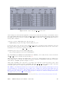
Table 1: JEM-X parameters and performance.
Energy range
Energy resolution†
Field of view (diameter)†
Angular resolution (FWHM)
Relative point source location error
Continuum sensitivity
for a single JEM-X unit
(isolated source on-axis)
Narrow-line sensitivity
(isolated source on-axis)
Timing resolution
3 – 35 keV
1/2
∆E/E = 0.40 × [(1/E keV) + (1/120 keV)]
◦
4.8 Fully illuminated
7.5◦ Half response
13.2◦ Zero response
30
10 (90% confidence radius for a 5σ isolated source)
1.2 × 10−4 ph cm−2 s−1 keV−1 @ 6 keV
1.0 × 10−4 ph cm−2 s−1 keV−1 @ 30 keV
for a 3 σ cont. detection in 105 s, ∆E = 0.5E
1.6 × 10−4 ph cm−2 s−1 @ 6 keV
1.3 × 10−4 ph cm−2 s−1 @ 20 keV
for a 3σ line detection in 105 s
122 µs (relative timing)
∼ 1 ms (absolute timing)
† The energy resolution is slowly changing (degrading) over time.
‡ At the half response angle the sensitivity is reduced by a factor 2 relative to the on-axis sensitivity.
ISDC – JEM-X Analysis User Manual – Issue 10.0
2
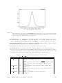
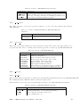
Figure 1:
2
2.1
JEM-X effective area with the mask taken into account. The dashed line shows the effective area before
the high voltage reduction and the full curve shows efficiency when taking into account the effect of the
electronic low-signal cutoff (approximately).
Instrument Description
The Overall Design
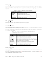
JEM-X consists of two identical coded-aperture mask telescopes co-aligned with the other instruments on
INTEGRAL . The photon detection system consists of high-pressure imaging Microstrip Gas Chambers
(MSGC) located at a distance of 3.4 m from each coded mask. Figure 2 shows a schematic diagram of one
JEM-X unit. A single JEM-X unit comprises 3 major subsystems: the detector, the associated electronics
and the coded mask.
The two JEM-X units have been used alternatively in the past, and are currently operated simultaneously.
The decision to use only one instrument at a time was made about three months after launch when a gradual
loss in sensitivity had been observed in both JEM-X units, due to the erosion of the microstrip anodes inside
the detector. By lowering the operating voltage, and thereby the gain of the detectors, the anode damage
rate has now been reduced to a level where the survival time of the detectors seems to be assured for a
further five year period. Only 6 anodes have been lost on JEM-X1 in all of 2006. Another 7 anode strips
have been lost on JEM-X1 in the first 8 months of 2007. For the complete, updated list of dead anodes see
http://www.spacecenter.dk/∼oxborrow/sdast/InstrConfig/JC.BadAnodes.txt
2.2
The Detector
Each JEM-X detector is a microstrip gas chamber with a sensitive geometric area of 500 cm2 per unit.
The gas inside the steel pan-shaped detector vessel is a mixture of xenon (90%) and methane (10%) at 1.5
bar pressure. The incoming photons are absorbed in the xenon gas by photo-electric absorption and the
resulting ionization cloud is then amplified in an avalanche of ionizations by the strong electric field near the
microstrip anodes. Significant electric charge is picked up on the strip as an electric impulse. The position
of the electron avalanche in the direction perpendicular to the strip pattern is measured from the centroid of
ISDC – JEM-X Analysis User Manual – Issue 10.0
3
Figure 2:
Left:Overall design of JEM-X, showing the two units, with only one of the two coded masks. Right:
functional diagram of one unit.
the avalanche charge. The orthogonal coordinate of an event is obtained from a set of electrodes deposited
on the rear surface of the microstrip plate (MSP).
The X-ray window of the detector is composed of a thin (250 µm) beryllium foil which is impermeable to
the detector gas but allows a good transmission of low-energy X-rays (see dashed curve in Fig. 1). the Be
window imposes an absolute lower limit of ' 3 keV on the energy of X-rays coming into the detector, and
hence it is meaningless to try to push the data analysis below this limit.
A collimator structure with square-shaped cells is placed on top of the detector entrance window. It gives
support to the window against the internal pressure and, at the same time, limits and defines the field of
view of the detector. The collimator is important for reducing the count rate caused by the cosmic diffuse
X-ray background. However, the presence of the collimator also means that sources near the edge of the
field of view are attenuated with respect to on-axis sources (see Fig.3). The materials for the collimator
(molybdenum, copper, aluminium) have been selected in order to minimize the detector background caused
by K fluorescence. Four radioactive sources are embedded in each detector collimator in order to calibrate
the energy response of the JEM-X detectors in orbit. For JEM-X1 two 55 Fe and two 109 Cd sources were
used. For JEM-X2 all four radioactive sources are 109 Cd. Each source illuminates a well defined spot on the
microstrip plate. 109 Cd emits 22 keV and 88 keV photons. 55 Fe produces one unresolved doublet at 6 keV.
The gain of the detector gas is monitored continuously with the help of these sources. Figure 4 shows the
collimator layout and the locations of the calibration sources. There is one calibration source for each anode
segment on the MSP. The 29.6 keV photons produced by Xe fluorescence can be detected all over the MSP
and are used for offline monitoring of the gain correction by the software, and also to produce instrument
model tables of the spatial gain (SPAG) variation across the detector plate. For the complete archive of
these offline analyses see: http://www.spacecenter.dk/∼oxborrow/sdast/GAINresults.html.
ISDC – JEM-X Analysis User Manual – Issue 10.0
4
Figure 3:
Figure 4:
Off axis response of JEM-X below 50 keV where the collimator walls are opaque. The thick line shows
the average transmission through the collimator considering all azimuth angles. The square pattern of
the collimator introduces an azimuthal dependence of the throughput with a minimum and a maximum
as indicated by the two thin curves (no response at ZRFOV indicated by dash-dot line).
Collimator layout. In this diagram the 4 calibration sources are situated on the upper side. The dimensions
are in mm, i.e. collimator length = 57 mm, radius = 130 mm
ISDC – JEM-X Analysis User Manual – Issue 10.0
5
Figure 5:
2.3
Illustration of the JEM-X coded mask pattern layout without the mechanical interface. The diameter of
the coded mask is 535 mm. The mask has a transparency of 25%.
Coded Mask
The mask is based on a Hexagonal Uniformly Redundant Array (HURA). For JEM-X a pattern composed
of 22501 elements with only 25% open area has been chosen. The 25% transparency mask actually achieves
better sensitivity than a 50% mask, particularly in complex fields with many sources, or in fields where
weak sources should be studied in the presence of a strong source. A mask with lower transparency also has
the advantage of reducing the number of events to be transmitted, while at the same time increasing the
information content of the remaining events. Considering the telemetry allocation to JEM-X, this means an
improved overall performance for the instrument, particularly for observations in the plane of the Galaxy.
The mask height above the detector ( 3.4 m) and the mask element dimension (3.3 mm) define together the
angular resolution of the instrument, in this case 3’. Figure 5 illustrates the JEM-X coded mask pattern.
ISDC – JEM-X Analysis User Manual – Issue 10.0
6
3
3.1
Instrument Operations
Telemetry Formats and Data Compression
JEM-X data can be transmitted in several different telemetry formats which vary in their information content
for position, energy or time and the required bandwidth per event. In addition, a “grey filter” mechanism
exists eliminating a fraction of the incoming events in a randomized way. The possible transmission settings
range from 32/32 to 1/32 of the incoming events. These mechanisms allow the instrument to cope with
sources of very different brightness despite its limited telemetry allocation.
For formats with poor time resolution (REST, SPEC) countrate data packets are also transmitted to provide
some data for timing analysis. However countrate data is not an independent data format.
For a given observation a primary and a secondary telemetry format are defined and they can be identical.
If the observed data rate is too high to be transmitted completely, first the grey filtering will be increased
to reduce the number of processed events. Should this not be sufficient the instrument will autonomously
switch to the secondary telemetry format, continuing to adapt the grey filter as necessary. For decreasing
input rates the instrument will reduce the filtering and possibly switch back to the primary format. All these
changes are driven by the filling status of an on-board buffer, the mechanism includes a certain hysteresis in
order to avoid rapid switching between formats.
The characteristics of primary and secondary telemetry formats are listed in Table 2. The default primary
format is Full Imaging and the default secondary format is Restricted Imaging. Note that in the Spectral
Timing format the actual spectral resolution will be slightly lower than that of the Full Imaging mode due
to spatial gain variations in the detector. It is recommended, however, that the full imaging format is used
both as primary and secondary format.
Table 2: Characteristics of the JEM-X Telemetry Packet Formats.
Format Name
Full Imaging
Restricted Imaging
Countrate
Spectral Timing
Timing
Spectrum
3.2
3.2.1
(FULL)
(REST)
()
(SPTI)
(TIME)
(SPEC)
Detector Image
Resolution
(pixels)
256 x 256
256 x 256
None
None
None
None
Timing
Resolution
1/8192s = 122µs
≤ 32 s
1/8 s = 125 ms
1/8192s = 122µs
1/8192s = 122µs
1/8s = 125 ms
Spectral
Resolution
(channels)
256
8
1
256
None
64
Events
per
packet
≤105
≤320
n/a
≤210
≤550
n/a
Energy Binning
PHA Binning
The energy values of the events provided in the telemetry are given as a bin number from 0 to 255. These are
non-linear groupings of the original 4096 bins of the on-board Analog to Digital Converter (ADC). While the
ADC channels are highly linear, the PHA bins are designed to be logarithmic so that the energy resolution
of the bins parallels that of the detector. The actual grouping of the ADC channels into PHA telemetry
bins is determined by a lookup table used by the Data Processing Electronics (DPE) to pack the telemetry.
After the high voltage reductions this table has been updated to match the changed ADC signal strengths.
See also Appendix B.3 for more details.
ISDC – JEM-X Analysis User Manual – Issue 10.0
7
3.2.2
PI Binning
The PI bin limits in keV have been defined so that the entire energy range (nominally 3–100 keV) is covered
and the binsize is a more or less constant fraction of the detector resolution. The PI binning table for the
Full Imaging mode with the highest number of bins (256) is shown in Table 3. See Appendix B.3 for more
details.
Table 3: Energy boundaries of the PI channels
PI
0
1
2
3
4
5
6
7
8
9
10
11
12
13
14
15
16
17
18
19
20
21
22
23
24
25
26
27
28
29
30
31
32
33
34
35
36
37
38
39
40
41
42
43
44
45
46
Emin
0.00
0.06
0.12
0.18
0.24
0.30
0.36
0.42
0.48
0.54
0.60
0.66
0.72
0.78
0.84
0.90
0.96
1.02
1.08
1.14
1.20
1.26
1.32
1.38
1.44
1.50
1.56
1.62
1.68
1.74
1.80
1.86
1.92
2.00
2.08
2.16
2.24
2.32
2.40
2.48
2.56
2.64
2.72
2.80
2.88
2.96
3.04
Emax
0.06
0.12
0.18
0.24
0.30
0.36
0.42
0.48
0.54
0.60
0.66
0.72
0.78
0.84
0.90
0.96
1.02
1.08
1.14
1.20
1.26
1.32
1.38
1.44
1.50
1.56
1.62
1.68
1.74
1.80
1.86
1.92
2.00
2.08
2.16
2.24
2.32
2.40
2.48
2.56
2.64
2.72
2.80
2.88
2.96
3.04
3.12
PI
86
87
88
89
90
91
92
93
94
95
96
97
98
99
100
101
102
103
104
105
106
107
108
109
110
111
112
113
114
115
116
117
118
119
120
121
122
123
124
125
126
127
128
129
130
131
132
Emin
6.24
6.32
6.40
6.48
6.56
6.64
6.72
6.80
6.88
6.96
7.04
7.12
7.20
7.28
7.36
7.44
7.52
7.60
7.68
7.76
7.84
7.92
8.00
8.08
8.16
8.24
8.32
8.42
8.52
8.62
8.72
8.82
8.92
9.02
9.12
9.22
9.32
9.42
9.52
9.62
9.72
9.82
9.92
10.08
10.24
10.40
10.56
ISDC – JEM-X Analysis User Manual – Issue 10.0
Emax
6.32
6.40
6.48
6.56
6.64
6.72
6.80
6.88
6.96
7.04
7.12
7.20
7.28
7.36
7.44
7.52
7.60
7.68
7.76
7.84
7.92
8.00
8.08
8.16
8.24
8.32
8.42
8.52
8.62
8.72
8.82
8.92
9.02
9.12
9.22
9.32
9.42
9.52
9.62
9.72
9.82
9.92
10.08
10.24
10.40
10.56
10.72
PI
171
172
173
174
175
176
177
178
179
180
181
182
183
184
185
186
187
188
189
190
191
192
193
194
195
196
197
198
199
200
201
202
203
204
205
206
207
208
209
210
211
212
213
214
215
216
217
Emin
17.90
18.16
18.42
18.68
18.94
19.20
19.46
19.72
19.98
20.24
20.50
20.76
21.02
21.28
21.54
21.80
22.06
22.32
22.58
22.84
23.10
23.36
23.72
24.08
24.44
24.80
25.16
25.52
25.88
26.24
26.60
26.96
27.32
27.68
28.04
28.40
28.76
29.12
29.48
29.84
30.20
30.56
30.92
31.28
31.64
32.00
32.36
Emax
18.16
18.42
18.68
18.94
19.20
19.46
19.72
19.98
20.24
20.50
20.76
21.02
21.28
21.54
21.80
22.06
22.32
22.58
22.84
23.10
23.36
23.72
24.08
24.44
24.80
25.16
25.52
25.88
26.24
26.60
26.96
27.32
27.68
28.04
28.40
28.76
29.12
29.48
29.84
30.20
30.56
30.92
31.28
31.64
32.00
32.36
32.72
8
47
48
49
50
51
52
53
54
55
56
57
58
59
60
61
62
63
64
65
66
67
68
69
70
71
72
73
74
75
76
77
78
79
80
81
82
83
84
85
3.12
3.20
3.28
3.36
3.44
3.52
3.60
3.68
3.76
3.84
3.92
4.00
4.08
4.16
4.24
4.32
4.40
4.48
4.56
4.64
4.72
4.80
4.88
4.96
5.04
5.12
5.20
5.28
5.36
5.44
5.52
5.60
5.68
5.76
5.84
5.92
6.00
6.08
6.16
3.20
3.28
3.36
3.44
3.52
3.60
3.68
3.76
3.84
3.92
4.00
4.08
4.16
4.24
4.32
4.40
4.48
4.56
4.64
4.72
4.80
4.88
4.96
5.04
5.12
5.20
5.28
5.36
5.44
5.52
5.60
5.68
5.76
5.84
5.92
6.00
6.08
6.16
6.24
133
134
135
136
137
138
139
140
141
142
143
144
145
146
147
148
149
150
151
152
153
154
155
156
157
158
159
160
161
162
163
164
165
166
167
168
169
170
10.72
10.88
11.04
11.20
11.36
11.52
11.68
11.84
12.00
12.16
12.32
12.48
12.64
12.80
12.96
13.12
13.28
13.44
13.60
13.76
13.92
14.08
14.24
14.40
14.56
14.72
14.88
15.04
15.30
15.56
15.82
16.08
16.34
16.60
16.86
17.12
17.38
17.64
10.88
11.04
11.20
11.36
11.52
11.68
11.84
12.00
12.16
12.32
12.48
12.64
12.80
12.96
13.12
13.28
13.44
13.60
13.76
13.92
14.08
14.24
14.40
14.56
14.72
14.88
15.04
15.30
15.56
15.82
16.08
16.34
16.60
16.86
17.12
17.38
17.64
17.90
218
219
220
221
222
223
224
225
226
227
228
229
230
231
232
233
234
235
236
237
238
239
240
241
242
243
244
245
246
247
248
249
250
251
252
253
254
255
32.72
33.08
33.44
33.80
34.16
34.52
34.88
36.16
37.44
38.72
40.00
41.28
42.56
43.84
45.12
46.40
47.68
48.96
50.24
51.52
52.80
54.08
55.36
56.64
57.92
59.20
60.48
61.76
63.04
64.32
65.60
66.88
68.16
69.44
70.72
72.00
73.28
74.56
33.08
33.44
33.80
34.16
34.52
34.88
36.16
37.44
38.72
40.00
41.28
42.56
43.84
45.12
46.40
47.68
48.96
50.24
51.52
52.80
54.08
55.36
56.64
57.92
59.20
60.48
61.76
63.04
64.32
65.60
66.88
68.16
69.44
70.72
72.00
73.28
74.56
81.92
The complete table can also be found in JMXi-IMOD-GRP structure, in extension JMXi-FBDS-MOD. The
Xe instrumental background line which is used to verify the gain calibration of the instrument should appear
in the channel 209.
ISDC – JEM-X Analysis User Manual – Issue 10.0
9
4
Performance of the Instrument
The properties described in the following have been derived in part from pre-flight calibration measurements
and modeling and in part from calibration observations in orbit. JEM-X has had major changes of its
configuration since launch, the most important being a reduction of the high voltages reducing the gas gain
from 1500 down to 500 for JEM-X 1 and to 750 for JEM-X 2. These changes also affect the instrument
performance.
4.1
Position Resolution
The position determination accuracy depends on the number of source and background counts and on the
position in the Field of View (FOV). Off-axis the collimator blocks some of the source photons and beyond
the fully coded FOV (FCFOV) the coding is incomplete.
Figure 6 shows the position resolution for a source on axis as function of energy. The cause of the degradation
below 10 keV is the signal-to-noise ratio of the front-end electronics. The energy dependence of the position
resolution above 10 keV is determined by the increase of the primary photoelectron range with energy. The
position resolution is slightly degraded compared to the ground calibrations.
Figure 6:
The calculated position resolution in the JEM-X 1 and JEM-X 2 detectors as a function of energy valid
after 2002-11-09 (JEM-X 1) and after 2002-11-12 (JEM-X 2).
ISDC – JEM-X Analysis User Manual – Issue 10.0
10
4.2
Energy Resolution
The energy resolution has been determined in the laboratory as
p
∆E/E(F W HM ) = 0.40 · 1/E[keV] + 1/120 keV.
This value has not been significantly affected by the gain change and the corresponding slight rise in importance of the electronic noise.
4.3
Background
The local radiation environment is mainly produced by two components: the diffuse X-ray background (DXB)
and cosmic rays (CR). Most of the latter are rejected on-board with a combination of pulse height, pulse
shape, anti-coincidence and “footprint” evaluation techniques. These techniques allow a particle rejection
efficiency of >99.9% with carefully tuned selection parameters. This high rate of background rejection has
ensured that there has been no significant increase in background events in the telemetry despite the steady
increase in the CR rate at Solar minimum.
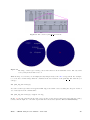
Figure 7 shows an actual background spectrum which is composed of the diffuse X-ray background, instrumental background due to the interactions with cosmic rays and three strong instrumental lines due to the
cooper and molybdenum in the collimator (8.04 keV and 17.4 keV) and Xe fluorescence from the detector
gas at 29.6 keV.
Figure 7:
Empty field background spectrum measured with the nominal detector gain of 1500 (left) compared to
the background spectrum with the reduced gain of 500 (right). After these measurements the rejection
criteria have been adjusted (2003-02-25), but no blank fields have been observed for a longer period since
then. The background has increased with about 10-15% at higher energies and with 20-30% below 10 keV
after the adjustment.
ISDC – JEM-X Analysis User Manual – Issue 10.0
11
4.4
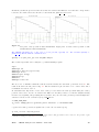
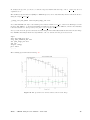
Sensitivity
The sensitivity achieved for source detection and flux determination also depends on the performance of the
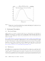
deconvolution software. Figure 8 shows the 3 σ detection limit as a function of observation time.
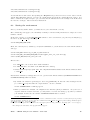
The changes in gas gain and corresponding changes in signal patterns led to a large fraction of events being
classified as background and rejected on-board until new selection criteria could be determined and uploaded
(2003-03-25, revolution 45). Even with the new optimized selection criteria the detector sensitivity below
5 keV is reduced.
Figure 8:
Source detection capabilities in the 3 to 10 keV (resp. 10 to 25 keV) band as function of effective
accumulated observation (exposure) time in JEM-X mosaic images corrected for dead time, grey filter and
vignetting effects. The thick solid curve is obtained from simulations where an isolated source must be
detected at 3σ in the deconvolved image. The dashed line represents the case where there are additional
sources in the field of view giving a background corresponding to a total of 1 Crab. Examples of actual
observations are given: the source 3C 273 and the other empty circles are instances of isolated sources,
while the crossed circles represent sources observed in the crowded Galactic Centre region. The σ-values
given in parentheses are obtained from a measure of the highest source pixel in significance mosaic maps
with default pixel size (1.5 arcmin).
ISDC – JEM-X Analysis User Manual – Issue 10.0
12
Part II
Data Analysis
5
Overview
The scientific analysis performed by the user on the data collected by the three high-energy instruments
on-board INTEGRAL has a lot of commonality, despite the various differences in detail. In a certain step,
for example, events are corrected for instrumental fingerprints, in another one events are binned into detector
maps, and in yet another step sky images are derived by image deconvolution.
In order to make this more transparent for scientists working with data from several instruments, so-called
Analysis Levels were identified by the ISDC and designated with unique labels. The order of these levels,
the detailed processing and the details of the outputs may differ across instruments, but in general, a given
level will mean similar tasks and similar outputs for JEM-X, IBIS, and SPI. The list of all levels is given in
the Introduction to the INTEGRAL Data Analysis [1]. For JEM-X the following levels have been defined:
Table 4: Overview of the JEM-X Scientific Analysis Levels.
Tasks
Description
COR
GTI
DEAD
CAT I
BIN I
IMA
SPE
LCR
BIN S
BIN T
IMA2
Data Correction
Good Time definition and handling
Dead Time derivation
Catalogue source selection for Imaging
Event binning for Imaging
Image reconstruction, source flux determination
Source spectra and response extraction (for XSPEC)
Source light curves extraction
Event binning for Spectral Analysis
Event binning for Timing Analysis
Creation of mosaic images and summary on sources found
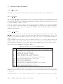
Figure 9 shows the Scientific Analysis overview. The details of each step are briefly discussed below.
COR – Data Correction (j correction)
Corrects science data for instrumental fingerprints such as energy and position corrections, as well
as flagging events of dubious quality. Look up tables of pre-flight corrections are used, as well as
tables of in-flight calibrations determined by offline analysis of science data, calibration spectra, and
instrumental background lines. Dynamic determination of known transient problems (e.g. hotspots on
the detector) is also done in this level. The majority of calibration tables are stored in the Instrument
Model group, JMXi-IMOD-GRP (with i = 1 and 2 for JEM-X1 and JEM-X2, respectively), but the
offline gain history Instrument Characteristics tables are stored separately in JMXi-GAIN-OCL data
structures. The latter are also located automatically by the OSA software just like the IMOD group.
GTI – Good Time Handling (j gti)
Good Time Intervals (GTIs) are used in the analysis to select only those data taken while the detector
was considered to work correctly. The corresponding data structures consist simply of a list of start
and stop times of those intervals considered “good”. Usually, these intervals are generated based on
the following data:
1. Housekeeping parameters which are compared with pre-set limits.
ISDC – JEM-X Analysis User Manual – Issue 10.0
13
Figure 9: Decomposition of the jemx science analysis script.
ISDC – JEM-X Analysis User Manual – Issue 10.0
14
2. The satellite stability as recorded in the attitude data.
3. Gaps (lost packets) in the telemetry flow.
In addition, this step excludes by default periods when the instrument configuration is not adapted
to the production of scientific works, either because of hardware problems or because of intentional
modifications of the instrument configurations for the purpose of testing and calibrations. These
periods are marked as ”bad time intervals”in the Instrument Characteristics data.
DEAD – Dead and Live Times (j dead time)
For each 8 second onboard polling cycle, this level calculates the dead time during which photons are
lost due to finite read in time of registers, event processing time, grey filter losses, buffer losses and
double event triggers.
CAT I – Catalogue Source Selection (j cat extract)
Selects a list of known sources from the given catalogue. Creates a source data structure, containing
source location and expected flux values.
BIN I – Event Binning for Imaging (j image binning)
Defines the energy bins to be used for imaging, selects good events within the GTI, and creates
shadowgrams. Works only on FULL and REST data (see Table 2).
IMA – Image Reconstruction (j imaging)
Generates sky images and performs search for significant sources. If sources are detected, a new source
data structure is created, including part of the information from the input catalogue concerning the
identified sources. Works only on FULL and REST data (see Table 2)
SPE – Spectra Extraction (j src extract spectra)
Extracts spectra for individual sources found at IMA step, and produces the specific response files
(ARFs) needed for spectral fitting with the XSPEC package. Works only on FULL data (see Table 2).
LCR – Extract Source Light Curves (j src extract lc)
Produces light curves for individual sources. Works only on FULL data (see Table 2)
BIN S – Event Binning for Spectral Analysis (j bin spectra)
Creates detector spectra, i.e spectra of all events recorded within the GTI are corrected for greyfilter,
ontime and deadtime. A series of spectra resolved in time or phase over a given period can be produced.
BIN T – Creates Detector Light Curves (j bin lc)
Creates binned lightcurves for entire detector area.
IMA2 – Mosaic Image Creation (j ima mosaic, src collect)
Generates mosaic sky images and creates the list of all found sources. Works only on FULL and REST
data (see Table 2)
Since October 18, 2004, all public INTEGRAL data are available including already the correction step, and
also the instrumental GTI and deadtime handling have been already performed at the science window level.
This allows to speed up the scientific analysis of JEM-X data as there is no need to redo the COR, GTI and
DEAD levels, but you can directly start JEM-X analysis from the CAT I level.
It is however recommended that users run the science analysis from the COR level onwards, especially after
downloading new software, and IMOD/IC files. This will undoubtedly give better results than the archived
data. Archived data necessarily fossilize our understanding of the instruments as it was at the time of the
archival processing and can therefore be several years out of date since our knowledge of the instruments,
and the software to process the data is still improving.
ISDC – JEM-X Analysis User Manual – Issue 10.0
15
6
Cookbook for JEM-X analysis
The Cookbook describes how to use the OSA JEM-X software. It covers the following steps:
• Setting up the analysis data
• Setting the environment
• Launching the analysis
• Interpreting the results
We assume that you have already successfully installed the ISDC Off-line Scientific Analysis (OSA) Software
version 10.0 (The directory in which OSA is installed is referred later as the ISDC ENV directory). If this is
not the case, look at the “Installation Guide for the INTEGRAL Off-line Scientific Analysis” [4] for detailed
help.
6.1
Setting Up the Analysis Data
In order to set up a proper environment, you first have to create an analysis directory (e.g jmx data rep)
and “cd” into it:
mkdir jmx_data_rep
cd jmx_data_rep
setenv REP_BASE_PROD $PWD
This working directory will be referred to as the REP BASE PROD directory in the following. All the data
required in your analysis should then be available from this “top” directory, and they should be organized
as follows:
• scw/ : data produced by the instruments (e.g., event tables) cut and stored by ScWs
• aux/ : auxiliary data provided by the ground segment (e.g., time correlations)
• cat/ : ISDC reference catalogue
• ic/ : Instrument Characteristics (IC), such as calibration data and instrument responses
• idx/ : set of indices used by the software to select appropriate IC data
The JEM-X example presented below is based on observations of the Crab from Revolution 102.
Part of the required data may already be available on your system1 . In that case, you can either copy these
data to the relevant working directory, or better, create soft links as follows
ln
ln
ln
ln
ln
-s
-s
-s
-s
-s
directory_of_ic_files_installation__/ic ic
directory_of_idx_files_installation__/idx idx
directory_of_cat_installation__/cat cat
directory_of_local_archive__/scw scw
directory_of_local_archive__/aux aux
1 For installation of the Instrument Characteristics files (OSA IC package) and the Reference Catalogues (OSA CAT package),
follow the instructions given in “Installation Guide for the INTEGRAL Data Analysis System” [4].
ISDC – JEM-X Analysis User Manual – Issue 10.0
16
JEM-X calibration files are continuously produced by the JEM-X Team for new revolutions. To be sure to
have all the latest calibrations, update your copy of the Instrument Characteristics each time you want to
analyse new data, using the rsync command:
rsync -Lzrtv isdcarc.unige.ch::arc/FTP/arc_distr/ic_tree/prod/
directory_of_ic_files_installation__
This command will download the Instrument Characteristics files (ic and idx directories) to your
directory_of_ic_files_installation__.
Then, just create a file ’jmx.lst’ containing the 2 lines:
scw/0102/010200210010.001/swg.fits[1]
scw/0102/010200220010.001/swg.fits[1]
which is the list of ScWs you want to analyse (technically, we call them DOLs - Data Object Locators -, i.e.
a specified extension in a given FITS file). 2
This file name ‘jmx.lst’ will be used later as an argument for the og create program (see section 6.5).
Alternatively, if you do not have any of the above data on your local system, or if you do not have a local
archive with the scw/ and the aux/ branch available, follow the next section instructions to download data
from the ISDC WWW site.
6.2
Downloading Your Data
To retrieve the required analysis data from the archive, go to the following URL:
http://www.isdc.unige.ch/integral/archive.
You will reach the W3Browse web page which will allow you to build a list of Science Windows (ScWs)
needed to create your observation group for OSA.
• Type the name of the object (Crab) in the ‘Object Name Or Coordinates:’ field.
• Click on the ’More Options’ button at the top or at the bottom of the web page.
• Deselect the ’All’ checkbox at the top of the Catalog table, and select the ‘SCW - Science Window
Data’ one.
• Press the ‘Specify Additional Parameters’ button at the bottom of the web page.
• Deselect the ‘View All’ checkbox (press twice on it) at the top of the Query table.
• Select ‘scw id’ and put the value ‘0102*’ (without the quotes) to specify all Scws from Revolution 102.
• Select ‘scw type’ and put the value ‘pointing’ (without the quotes), or simply ‘po*’ to get only pointings.
• Press the ‘Start Search’ button at the bottom of the web page. At this point, you should be at the
Query Results page with all the Scws available for revolution 102.
• Sort the ‘Scw id’ column by clicking on the left arrow below the column name. You can then select
the two Scws we are interested in, i.e 010200210010 and 010200220010.
Press the ‘Save SCW list for the creation of Observation Groups’ button at the bottom of that table
and save the file with the name ‘jmx.lst’. The file name ‘jmx.lst’ will be used later as an argument for the
og_create program (see section 6.5). In this file, you should find the 2 lines:
2 When an analysis script asks you to specify the DOL, you should specify the path of the corresponding FITS file, and the
corresponding name or number of the data structure in square brackets(do not forget that numbering starts with 0!). See more
details in the Introduction to the INTEGRAL Data Analysis [1].
ISDC – JEM-X Analysis User Manual – Issue 10.0
17
scw/0102/010200210010.001/swg.fits[1]
scw/0102/010200220010.001/swg.fits[1]
You should then download the data pressing the ’Request data products for selected rows’ button. In the
‘Public Data Distribution Form’, provide your e-mail address and press the ‘Submit Request’ button. You
will be e-mailed the required script to get your data and the instructions for the settings of the IC files and
the reference catalogue. Just follow these instructions.
6.3
Setting the environment
Before you run any OSA software, you must also set your environment correctly.
The commands below apply to the csh family of shells (i.e csh and tcsh) and should be adapted for other
families of shells3 .
In all cases, you have to set the REP BASE PROD variable to the location where you perform your analysis (e.g
the directory jmx data rep). Thus, type:
setenv REP_BASE_PROD $PWD
Then, if not already set by default by your system administrator, you should set some environment variables
and type:
setenv ISDC_ENV directory_of_OSA_sw_installation
setenv ISDC_REF_CAT $REP_BASE_PROD/cat/hec/gnrl_refr_cat_0031.fits\[1]
source $ISDC_ENV/bin/isdc_init_env.csh
The idea is to:
• set ISDC ENV to the location where OSA is installed
• set ISDC REF CAT to the DOL of the ISDC Reference Catalog
• run the OSA set-up script (isdc init env.csh) which initializes further environment variables relative
to ISDC ENV.
Besides these mandatory settings, there are two optional environment variables (COMMONLOGFILE and
COMMONSCRIPT) which are useful.
• By default, the software logs messages to the screen (STDOUT). To have also these messages in a file
(i.e common log.txt) and make the output chattier4 , use the command:
setenv COMMONLOGFILE +common_log.txt
• When you launch the analysis, the Graphical User Interface (GUI) is launched. As your level of
expertise with the software increases, you may wish to not have the GUIs pop up when you launch
your analysis. In this case, the variable COMMONSCRIPT must be defined:
setenv COMMONSCRIPT 1
3 If the setenv command fails with a message like:‘setenv: command not found’ or ‘setenv: not found’, then you are probably
using the sh family. In that case, please replace the command ‘setenv my variable my value’ by the following command sequence
‘my variable=my value ; export my variable’
In the same manner, replace the command ‘source my script’ by the following command ‘. my script’ (the ‘.’ is not a typo!).
4 For
example, the exit status of the program will now appear.
ISDC – JEM-X Analysis User Manual – Issue 10.0
18
When the GUI is disabled, parameters can be specified on the command line typing ’name = value’
after the script name.
To revert and have the GUI again, unset the variable:
unsetenv COMMONSCRIPT
6.4
Useful to know!
In this section we report some general information that might be useful when running OSA software. Most
of these information can be found also in the IBIS Cookbook5 .
• How do I get some help with the executables?
All the available help files are stored under $ISDC ENV/help. To visualize a help file interactively
type tool name --h once your environment is set (i.e. the command which tool name should return
the path to it).
• Where are the parameter files and how can I modify them?
All the available executables for the analysis of INTEGRAL data are under $ISDC ENV/bin. The
corresponding parameter files are stored under $ISDC ENV/pfiles/*.par. The first time you launch
a script, the system will copy the specific tool.par from $ISDC ENV/pfiles/ to a local directory
(/user name/pfiles/). The parameter file in the local directory is the one used for the analysis and is
the one you can modify. If this parameter file is missing (e.g. you have deleted it), the system will
just re-copy it from $ISDC ENV/pfiles/ as soon as you launch the script again. The system knows
what to copy from where thanks to the $PFILES environment variable that is also used in FTOOLS
(http://heasarc.gsfc.nasa.gov/ftools/). Each parameter is characterized with a letter that specifies the
parameter type, i.e:
“q” (query) parameters are always asked to the user
“h” (hidden) parameters are not asked to the user and the indicated value is used
“l” (learned) parameters are updated with the user’s value during the use of the program.
The GUI is a fast and easy way to change the parameters, see also the explanation at the end of this
section.
• What are groups and indices?
The ISDC software makes extensive use of groups and indices. While it is not necessary to grasp all
the details of these concepts, a basic understanding is certainly quite useful.
As implied by their names, ”groups” make possible the grouping of data that are logically connected.
Groups can be seen as a kind of data container, not completely unlike standard directories. At ISDC,
we create separate groups for each pointing, in which we store the many different data types produced
by INTEGRAL and its instruments. The user then only has to care about one file, the group, many tens
of files being silently included. Several pointings (the “Science Window Groups”) can be arbitrarily
grouped into bigger groups (the “Observation Group”) to select data very efficiently according to the
user’s needs.
Indices are a special kind of groups, which differ only in the fact that all the the data sets they contain
are similar and that the indices know the properties of the data sets they contain. Indices are a kind of
poor man’s database. For example, an imaging program creates several images of different types (flux
map, significance map,...) in different energy bands. These images are stored in an index, in which
the image type and energy band information is replicated. ISDC software is then able to select very
efficiently the needed images. The user can also make use of the indices; just by looking at the index
(for instance using “fv”), the user can identify immediately the content of each image.
• Why do I need “[1]” after a FITS file name?
A FITS file can have many extensions and sometimes it is necessary to specify as input to a given parameter not the file name alone (file.fits) but the extension too (file.fits[1], or file.fits[2],
5 The
IBIS Cookbook is available at the URL http://www.isdc.unige.ch/integral/analysis
ISDC – JEM-X Analysis User Manual – Issue 10.0
19
etc). The file name with a specified data structure (extension) is called DOL (Data Object Locator). When you modify the parameter file itself (see above) or use the GUI, the extension will be
correctly interpreted in the file.fits[1] case. On the command line though, the normal CFITSIO
and FTOOLS rules apply, i.e. you have to specify it as one of the following
file.fits\[1]
file.fits+1
"file.fits[1]".
Note that if no extension is specified explicitly then the first one ([1]) will be used by default.
• What are the general functionalities of the GUI?
When you launch the analysis, by default the GUI is launched, providing an opportunity to set the
values of all desired parameters, see Figure 10. On the right side of the panel you see the following
buttons:
– Save as – With the “Save As” - button a file is created. This file stores all parameters as they are
currently defined in the GUI as a command line script. This file is an executable one and calling
it from the command line will launch the instrument analysis program with the parameters as
they were defined in the GUI.
– Load With the “Load” - button a previously saved file (see “Save As”) can be read and the GUI
will update all parameters with the values as they are defined in the loaded file.
– Reset With the “Reset” - button the parameters in the GUI will be reset to the default values
as they are defined in the parameter file of the instrument analysis program and stored in the
$ISDC ENV/pfiles directory.
– Run With “Run” - button the analysis is launched.
– Quit With “Quit” - button you quit the program without analysis launch.
– Help With “Help” - button the help file of the main script is opened in a separate window.
– hidden With the “hidden” - button you have an access to the hidden parameters with values
defined by the instrumental teams. Change them with care!
The environment variable COMMONSCRIPT is used to disable/enable the GUI (see section 6.3).
6.5
A Walk Through the JEM-X Analysis
After setting up the data and the environment, you are ready to call the analysis script on the Crab region
observations defined above and stored in the jmx.lst file.
Firstly, create an Observation Group (see the description of the executable og create in the “Toolbox” and
“Data Analysis” sections of the Introduction to the INTEGRAL Data Analysis [1]):
og_create idxSwg=jmx.lst ogid=crab baseDir="./" instrument=JMX2
As a result, the directory $REP BASE PROD/obs/crab will be created6 . It contains the files og jmx2.fits
and swg idx jmx2.fits as well as the subdirectory scw necessary for the analysis. In the latest version of
og create, the file indicated in idxSwg is automatically interpreted as a fits file when the name includes a
“+” or “[” sign.
6.6
Examples of Image Creation
Now you can go to the directory created with og create and start the analysis
6 To create the structure for both JemX units at the same time, it is possible to call og create only once, with the parameter
instrument=JMX1,JMX2.
ISDC – JEM-X Analysis User Manual – Issue 10.0
20
cd obs/crab
jemx_science_analysis startLevel="COR" endLevel="IMA" nChanBins=-4 jemxNum=2
The above command launches the analysis which will run from the Correction step (startLevel="COR") up
to the image creation level (endLevel="IMA"). It is important to specify that we are interested in the second
of JEM-X instruments: jemxNum=2. nChanBins parameter specifies the energy binning (see section 6.7.2 for
details).
At the beginning the script launches the GUI (Fig. 10) and you can check the parameter settings (the full
Figure 10: GUI for JEM-X science analysis.
list of the parameters is given in Table 60). Only the most important parameters (shown in bold in Table 60)
appear within the main panel of GUI. To access the other “hidden” parameters click on the button “hidden”
on the right side of the panel.
The behaviour of the IMA step has changed between OSA 7 and OSA 8. This is because fluxes have now
to be extracted using the IMA step, in order to profit from the vast improvement in the modelling of the
JEM-X instruments in OSA 8. Therefore, the normal behaviour is that IMA does not produce images for
the binning specified under ”General Binning Tasks”.
By default, jemx science analysis creates images in the 3 energy ranges: 3-7 keV, 7-11 keV and 11-20 keV,
which corresponds to the images used for optimal source detection. While this can be changed by the user,
this should not be modified in normal analyses. To generate images in arbitrary energy bands, see section
6.6.7.
In the upper frame of the front panel called “General” you can choose at which level you want to start and
stop the script execution. In the Overview chapter you have seen that there are different processing levels
of the analysis. You can choose to run only some of them. The default settings of the jemx science analysis
script are
startLevel="COR" start the script at COR level,
endLevel="IMA2"
stop the script at IMA2 level.
It is advisable always to start with level COR. This will allow the processing of the data using the latest
knowledge of the calibration of the instrument.
ISDC – JEM-X Analysis User Manual – Issue 10.0
21
If you want to skip some levels, click on the “hidden” button on the right of the GUI panel to access the
whole set of jemx science analysis parameters. In the frame “General” you find the skipLevels parameter.
However, be always careful while setting this parameter – levels often depend on the previous ones, so make
sure that your selection makes sense. Another useful hidden parameter IMA skyImagesOut in the IMA section
enables you to choose the types of images which you want to output7 . The checkbox IMA detImagesOut
enables you to output also the images in the pre-defined energy bands used by the j ima iros for the source
search. This option is not recommended if you want to extract a spectrum from the mosaic image later.
In the middle of the GUI front panel you have a possibility to choose a “user input catalog” (the parameter
CAT I usrCat). At the moment you can leave it empty (the software will use the general INTEGRAL source
catalog for the analysis). However, for the correct extraction of spectra and lightcurves of the sources it is
recommended to create a “user catalog” with the positions of the sources for which you plan to extract the
spectra and/or the lightcurves. We will come back to this in the following sections (and sect. 7.5).
Once you are satisfied with the settings, save them by pressing the “Save As” button at the front panel of
GUI and then press “Run” to start the data reduction.
6.6.1
Results from the Image Step
After jemx science analysis finishes its operation, the results are stored separately for each ScW of the observation group. They are located in the subdirectories named scw/RRRRPPPPSSSF.001/ (where RRRRPPPPSSSF
is the number of the ScW).
Go to one of these directories and have a look at the files
cd scw/010200210010.001/
ls
This is the output from all the processing steps done by the script.
The output image is jmx2 sky ima.fits. You can check it using e.g. fv:
fv jmx2_sky_ima.fits
You will find that this file contains 7 extensions: the index of all images, 3 cleaned sky images (RECONSTRUCTED
type), and 3 variance maps, one for each of the 3 selected energy bands (see Fig. 11).
In the file jmx2 srcl res.fits you find a list of all found sources, the energy bands, and the derived flux
values, and in the file jmx2 srcl cat.fits the list of the sources in the input catalog. You can see that
most of the catalog sources were not found, as they are too weak. When you run the lightcurve and spectra
extraction steps the results would be produced for all sources listed in jmx2 srcl res.fits.
Please note that with OSA10 the count rates are scaled to one cm2 , while until OSA9 the count rates were
scaled to one dm2 .
There is a nice way to locate the found sources as well as the catalog sources on the sky image. To do it use
the utility cat2ds9:
cat2ds9 jmx2_srcl_res.fits\[1] found.reg symbol=box color=red
cat2ds9 jmx2_srcl_cat.fits\[1] cat.reg symbol=circle color=white
(to find out more about this program type cat2ds9 --h in the command line). With the help of the above
two commands the two files found.reg and cat.reg are created. They contain the lists of all the found
sources and all the catalog sources, respectively.
7 Several types of images may be produced: the vignetting-corrected intensity image, called RECONSTRUCTED, the variance
image VARIANCE, RECTIFIED (raw intensity image), RESIDUAL (residuals left after removing all found sources) and EXPOSURE (the
exposure map).
ISDC – JEM-X Analysis User Manual – Issue 10.0
22
Figure 11: The content of jmx2 sky ima.fits file.
Figure 12:
The image of Crab region. Catalog sources in the FOV are shown with white circles. The only found
source (Crab) is shown with a red box.
With the help of ds9 viewer you can display the sky images in any of the three energy bands. For example,
to look at the 7–11 keV image which is contained in the 5th extension of the jmx2 sky ima.fits file you
can type
ds9 jmx2_sky_ima.fits\[5]
You can load the region files cat.reg and found.reg created with cat2ds9 by using the “Region” menu of
ds9 or directly from the command line:
ds9 jmx2_sky_ima.fits\[5] -region cat.reg
In Fig. 12, the left panel shows the Crab region in the second energy band (7–11 keV) with the catalog
sources, and the right one – the same region with the found sources (Science Window 010200210010).
ISDC – JEM-X Analysis User Manual – Issue 10.0
23
6.6.2
Weak Sources and Sources at the Edge of the FOV
The source acceptance is based on a positive detection in at least two energy bands. However, a strong
source that only appears in a single energy band may also be accepted. Such an acceptance is based on
the parameter ’IMA detSigSingle’ (Note, however, that it is NOT a statistical sigma). The default value is
12 which prevents most of the spurious detections to be accepted. However, if the aim is to find the weak
sources the value can be reduced to e.g. 10. Still lower values will probably cause too many spurious sources.
The number of detector pixels that contribute to the sky image decreases towards the edge of the FOV. That
implies on one hand that spurious sources are more likely to occur at the edge and on the other hand that
sources located there will be less reliable as is reflected in the relative error of the flux determination.
6.6.3
PIF-cleaning of images around strong sources
The image generating algorithm used by default in the JEM-X Scientific Analysis assigns equal weights to
all active detector pixels. This allows to assign errors to the source fluxes with reasonable accuracy. For
observations where the diffuse background is dominating the count rate this imaging technique appear as
the best approach.
However, when bright sources are in the field of view and significantly increases the global count rate the
situation changes. Due to the presence of the 25% open mask, the counts from a source will affect strongly at
most a quarter of the detector pixels, but in those it may strongly dominate the pixel counts. Consequently,
it could be advantageous to reduce the weight of pixels illuminated by a bright source when generating
images intended for detection of weak sources. Since we are always operating with very few counts in the
individual detector pixels the pixel counts cannot be used to determine the relevant weights, instead the
weights are derived from the pixel illumination functions (PIF) used in the source fitting procedure. A new
”PIF-weighted” image generation algorithm based on the above considerations have been implemented and
is available in the new JEM-X Scientific Analysis package.
PIF imaging can be activated by including the string ”PIF” in the IMA skyImagesOut string accessible from
the jemx science analysis GUI as one of the ”hidden” parameters.
(Example: IMA_skyImagesOut="PIF,RECONSTRUCTED,VARIANCE". Abbreviations as e.g. "PIF,RECON,VARIA"
can also be used) .
The PIF-imaging technique improves the visibility of weak sources in crowded fields like the Galactic Centre
or in the neighborhood of strong sources like the Crab or GRS 1915+105 (Figure 13).
NOTE HOWEVER, THAT PIF-IMAGES SHOULD NOT BE USED WITH ”mosaic spec”! FOR THE
TIME BEING IT IS NOT RELIABLE TO EXTRACT SPECTRA WITH ”mosaic spec”(6.7.7) FOR STRONG
SOURCES (SOURCES STRONG ENOUGH TO BE DETECTED IN SINGLE SCIENCE WINDOWS)
FROM PIF IMAGES - OR FROM MOSAICS BASED ON PIF IMAGES.
THE FITTED FLUXES in ”src ls res” SHOULD BE USED TO EXTRACT SPECTRA FOR STRONG
SOURCES, THESE FLUXES ARE NOT AFFECTED BY THE PIF-IMAGING OPTION.
6.6.4
The Mosaic Image
The IMA2 level produces JEM-X mosaic images by combining all the individual j ima iros images from the
different science windows gathered in the observation group. The combined images have longer exposure
time. As a consequence, weaker sources which are not visible in single ScW may appear in the mosaic images.
In what follows we consider an example of a JEM-X mosaic of the Galactic Center region for the revolution
0053 in March 2003. You can browse through the INTEGRAL data archive and check that within this
revolution the pointings which have the Galactic Center within the JEM-X2 FOV are
scw/0053/005300410010.001/swg.fits[1]
scw/0053/005300420010.001/swg.fits[1]
ISDC – JEM-X Analysis User Manual – Issue 10.0
24
Figure 13:
Left: Mosaic from conventional images centered on the strong source GRS 1915+105. Right: Mosaic
from PIF images in the same region of the sky.
scw/0053/005300490010.001/swg.fits[1]
scw/0053/005300510010.001/swg.fits[1]
scw/0053/005300580010.001/swg.fits[1]
scw/0053/005300590010.001/swg.fits[1]
scw/0053/005300650010.001/swg.fits[1]
scw/0053/005300660010.001/swg.fits[1]
scw/0053/005300670010.001/swg.fits[1]
scw/0053/005300680010.001/swg.fits[1]
scw/0053/005300740010.001/swg.fits[1]
scw/0053/005300750010.001/swg.fits[1]
scw/0053/005300760010.001/swg.fits[1]
scw/0053/005300820010.001/swg.fits[1]
Save the above list to the file mos.lst. To produce the mosaic image of these pointings you have first to
create the corresponding observation group mos using the og create tool, as has been explained above, and
run the jemx science analysis up to the IMA level.
cd $REP_BASE_PROD
og_create idxSwg=mos.lst ogid=mos baseDir="./" instrument=JMX2
cd obs/mos
jemx_science_analysis startLevel="COR" \
endLevel="IMA" jemxNum=2
Next, to produce the mosaic from the intensity images for each energy band as obtained at the IMA level,
you have to run the jemx science analysis script at IMA2 level only:
jemx_science_analysis startLevel="IMA2" endLevel="IMA2" jemxNum=2
Again, do not forget to specify which of the JEM-X instruments you are interested in (jemxNum=2 in our
case). By default, “intensity” (RECONSTRUCTED), “variance”, “significance” and “exposure” mosaic
images will be produced.
The same result can be obtained calling jemx_science_analysis only once, from startLevel="COR" to
ISDC – JEM-X Analysis User Manual – Issue 10.0
25
Figure 14: The content of jmx2 obs res.fits file.
endLevel="IMA2", eventually skipping the intermediate levels with the command skipLevels="LCR, SPE,
BIN S, BIN T".
Apart from the mosaic images, the output of the IMA2 level contains a collection of the results from the
individual science windows which is contained in the file jmx2 obs res.fits. Its content is shown in Fig. 14.
With the help of cat2ds9 command you can produce a region file found.reg to locate these sources at the
mosaic image:
cat2ds9 jmx2_obs_res.fits\[1] found.reg symbol=circle color=white
Note that since the same sources can be found in many ScWs you can have one and the same source repeated
several times in the resulting region file.
You can look at the content of the resulting mosaic images contained in the file jmx2 mosa ima.fits with
fv and display them with ds9 exactly as you did with the images from individual ScWs (see Fig. 15 for the
example of image in 7–11 keV energy band). In this figure you can see the sources found in single ScW
analysis shown with white circles. One can see that two additional sources, which were not detected in the
single ScWs, appear in the mosaic image (the sources shown by the green crosses).
If you are interested only in a particular region of the mosaic you can “zoom” on a given position in
the sky running jemx science analysis with additional parameters IMA2 RAcenter, IMA2 DECcenter and
IMA2 diameter which will specify the position of the center and the diameter (in degrees) of the resulting
mosaic image. To do so, first move the existing images8 :
mv jmx2_mosa_ima.fits jmx2_mosa_ima_original.fits
mv jmx2_obs_res.fits jmx2_obs_res_original.fits
Remember that the images have to be also removed from the observation group. This can be done by the
following command:
8 For
more details on how to re-run the analysis see sections 7.3
ISDC – JEM-X Analysis User Manual – Issue 10.0
26
Figure 15:
The mosaic image of the Galactic Center region for revolution 0053 in the 7–11 keV energy band (signifcance map).
dal_clean og_jmx2.fits+1
Now re-run the analysis script:
jemx_science_analysis startLevel="IMA2" endLevel="IMA2" jemxNum=2 \
IMA2_diameter=5.0 IMA2_RAcenter=266.4 IMA2_DECcenter=-29.0
(we have chosen to center the image on the Galactic Center position here).
If you want to produce a mosaic image only for a specific energy band you can pass the minimal and maximal
energies of the selected energy band to the jemx science analysis through the parameters IMA2 eminSelect
and IMA2 emaxSelect. Note that the energies have to be the same as defined previously in chanLow and
chanHigh.
To get the largest possible output mosaic in equatorial coordinates the parameters ”radiusSelect” and ”diameter” must both be set to -1. A better way, available with OSA v.10.0, is to use the Aitoff-Hammer
projection (in galactic coordinates) by setting the option AITproj. The latter enables the mosaicking of
large parts of the sky, such as for the Galactic Plane Scans, without distortion of the map (an example is
in Fig. 16). This new feature can be activated setting the parameter IMA2_AITproj="yes". The command
should be therefore as follows:
jemx_science_analysis startLevel="IMA2" endLevel="IMA2" jemxNum=2 IMA2_AITproj="yes"
The resulting AIToff mosaics are expected to be mapped in the Galactic plane, and are therefore oriented
in galactic, rather than equatorial, coordinates. To produce a mosaic over the whole sky you will need
to decrease the resolution of the image by increasing the pixel size (cdelt) at least to 0.075 degree. The
computation in AIToff-Hammer projection can take approximately 10% more CPU-time; and the resulting
file can have a rather large dimension (for example ∼1G). In this case a simple solution can be to compress
the file (e.g. with gzip) and to work directly with the compressed file (ds9 as well as other HEASOFT tools
are able to work directly with the compressed file).
ISDC – JEM-X Analysis User Manual – Issue 10.0
27
Figure 16:
6.6.5
The mosaic image of the Galactic Plane Scan observation of revolution 399 in the 3–10 keV energy band,
obtained in AIToff-Hammer projection.
Combining JEMX-1 and JEMX-2 mosaic images
j ima mosaic can combine JEM-X mosaics, provided that they have been obtained in the same energy bands,
for the same sky area and in the same projection. As for the simple mosaic image the user may specify
the coordinates of the center of the image (RAcenter and DECcenter parameters), as well as its size and
resolution (diameter and cdelt parameters9 ), when creating the mosaics. Any mix, however, of JEMX-1
and JEMX-2 mosaics is allowed.
As an example, let us create a mosaic image of the Galactic Center region, which combines the JEMX-2
mosaic (see previous sub-section) with the JEMX-1.
To combine mosaics, these must be attached in a group, so the first step is to create an empty group:
dal_create obj_name=jemx_mosaics.fits template=""
This uses the default template, which is a standard group. Next, we need to attach the mosaics:
dal_attach jemx_mosaics.fits obs1/jmx1_mosa_ima.fits\
obs2/jmx1_mosa_ima.fits obs3/jmx2_mosa_ima.fits ""
The final "" is necessary to signal to dal attach that there are no more data structures to attach. Up to five
data structures can be attached with a single dal attach commands. Additional extensions can be added by
issuing another dal attach command.
The combination of the mosaic is then very easily performed using the command:
j_ima_mosaic inObsGrp=jemx_mosaics.fits outfile=combined_mosaic.fits moscomb=y radiusSelect=-1
Combined JEMX-1 and JEMX-2 mosaics have the same structure as JEMX-1 ones, with EXTNAME=”JMX1MOSA-IMA”.
6.6.6
Finding Sources in the Mosaic Image
j ima src locator is a tool to locate point sources in an image. Since OSA-7 it is included in the OSA
distribution but is not part of the pipeline. This tool can be used to search for the gaussian excesses in the
mosaic image (but not to identify the detected sources at the moment).
9 For
details on j ima mosaic parameters see sections 8.11.1 and Appendix D
ISDC – JEM-X Analysis User Manual – Issue 10.0
28
Figure 17: The content of the jmx2 sloc res.fits file.
As an example, let us find all the significant excesses in the 7-11 keV mosaic image of the Galactic Center
region. We assume that in the mosaic image jmx2 mosa ima.fits the intensity map is in the extension 2 and
the significance is in the extension 4 (which is the case if the default value of IMA skyImagesOut parameter
is used). The command
j_ima_src_locator inDOL=jmx2_mosa_ima.fits\[2] \
sigDOL=jmx2_mosa_ima.fits\[4] outFile=jmx2_sloc_res
produces the list of the detected sources jmx2 sloc res.fits. In this file all the significant sources in
the mosaic image are listed. However, they are not identified with the known sources. To do the source
identification, you can use the q identify srcs script:
q_identify_srcs srcl_cat_dol="$ISDC_REF_CAT"\
srcl_res_dol=jmx2_sloc_res.fits instrument=5
(use instrument=4 for JEMX-1 and instrument=5 for JEMX-2) . As a result, the list of sources in the file
jmx2 sloc res.fits looks like it is shown in Fig. 17.
When inspecting the result the user might want to get rid of (too many) spurious sources or include more
sources that seem to be present. To achieve the latter the parameter ’maxNumSrcs’ must have an adequate
value and the ’detsigMin’ parameter might be lowered.
Analogously ’detsigMin’ can be increased to avoid false sources and there is some help in the log file to find
a reasonable value. Giving a negative ’detsigMin’ will cause j ima src locator to apply a limit of the first
found histogram value exceeding one plus the absolute value of the given ’detsigMin’.
The JEM-X coded mask has an almost non-cyclic pattern, which ensures imaging artifacts (ghost sources)
are particularly rare. Nevertheless in some peculiar cases, a bright source inside the FOV might cause the
presence of ghosts in the mosaic. These artifacts appear at 8.32 degrees from the bright source. To verify
that a ’New Source’ in the sloc res file is not instead a ghost, a simple test consists in checking whether there
are bright sources at 8.3 deg from it in the FOV10 .
10 If
you encounter a doubtful case, you can contact the help desk at http://www.isdc.unige.ch/integral/support/helpdesk
ISDC – JEM-X Analysis User Manual – Issue 10.0
29
6.6.7
Making images in arbitrary energy bands
IMA can use the general energy binning parameters nChanBins, chanLow and chanHigh to generate images
(note however that these parameters always determine the energy binning in the spectral extraction step,
SPE). To use these parameters at the IMA step, click on the “hidden” button and choose the “IMA” tab. Put
the IMA_detImagesOut to No and IMA_userImagesOut to Yes. If you run the IMA step with such parameter
settings, jmxi sky ima.fits will contain sky images for all bins specified by “General Binning Parameters”.
The mosaic image produced at the IMA2 level will also use these energy bins.
6.7
Source Spectra Extraction
Two spectral extraction algorithms can be used to extract the spectrum of a JEM-X source: the “standard”
spectral extraction carried out at the SPE level (discussed in section 6.7.1), and the spectral extraction from
mosaic images (discussed in section 6.7.7). Both of them originate from the imaging step.
WARNING: with OSA10, the count rates are scaled to one cm2 , while until OSA9, the count rate was scaled
to one dm2 .
6.7.1
Spectral Extraction at SPE level
The “standard” spectral extraction procedure is carried out at the SPE level of the jemx science analysis
script by re-formatting the source fluxes found at the IMA step. The file jmx2 srcl res.fits serves as
input for the spectral extraction in each ScW. It is important to note, however, that j ima iros will always
find a little bit different source positions in different ScWs. The deviation of the found source position from
the true one may lead to an error in determination of the source spectrum. To avoid this difficulty it is
recommended to create a “user catalog” with the names and positions of the sources for which you want to
extract the spectra11 .
For example, in the considered case, the source of interest is the Crab and one can just copy the corresponding
line from the general reference catalog:
fcopy "${ISDC_REF_CAT}[NAME==’Crab’]" user_cat.fits
In the new user cat.fits file you have to change the FLAG column to 1: in this case jemx science analysis
would directly copy the source position information to the jmx2 srcl res.fits after IMA step (see Sections
6.7.6 and 8.6.1 for an explanation on the possible FLAG values).
6.7.2
Energy binning definition
The user must now specify all the bins (s)he wants in the spectra, using nChanBins, chanMin and chanMax
parameters. As this can be tedious, standard binnings are provided by setting nChanBins to be < 1. In
this case IMA extracts fluxes in 2−nChanBins bins, i.e. a value nChanBins=0 results in a single wide energy
bin, while a value of -4 results in production of 16-channel spectra. The smallest allowed value is -6,
corresponding to the 64-channel spectra. Table 5 shows the standard energy bins up to 16 channels.
6.7.3
Spectral response generation
For spectral analysis, a response redistribution function (RMF) should be generated according to the spectral
binning specified by the user. The j rebin rmf script allows to do this very easily. There are several ways to
11 To force the use of the catalogue positions the JMXi-SRCL-RES table must be manipulated by e.g an ftool to update
columns RA OBJ, DEC OBJ. For more details see section 9.
ISDC – JEM-X Analysis User Manual – Issue 10.0
30
nChanBins
0
-1
-2
-3
-4
chanLow
46
46 130
46 77 130 175
46 59 77 102 130 153 175 199
46 52 59 68 77 89 102 117 130
141 153 165 175 187 199 211
chanHigh
223
129 223
76 129 174 223
58 76 101 129 152 174 198 223
51 58 67 76 88 101 116 129
140 152 164 174 186 198 210 223
Table 5: Standard energy binning.
run this script. The user can specify the bins individually, generate a bin list in a text file (see FTOOLS
rbnrmf explanations). For example,
j_rebin_rmf chanMin="46 77 130 175" chanMax="76 129 174 233" jemx_num=2
or
j_rebin_rmf binlist=mybins.txt outfile="jmx1_rmf_mybins.fits"
Otherwise, it is possible to use pre-defined standard binnings matching those set with nChanBins< 1:
j_rebin_rmf binlist=STD_016
(matches nChanBins=-4). As a result, a file jemx rebinned rmf.fits (unless a different file name has been
specified through outfile), which contains the rebinned RMF will be produced.
Note that jemx num=1 is the default value. The output file name (default jemx rebinned rmf.fits) can be
set through the outfile parameter. It is convenient to create an RMF before the spectral analysis so that
one can just pass the rebinned RMF to the analysis scripts. In this way, the fits files with the spectra will
automatically contain a link to the correct RMF.
6.7.4
Individual Science Windows Spectra
Let us first proceed with the spectral extraction using the source positions found at the IMA step. In
our example only the Crab was found by the imaging analysis, so the spectral analysis will generate only
the spectrum of the Crab if you run the script with default values (assuming you run j rebin rmf in your
$REP BASE PROD directory):
cd $REP_BASE_PROD/obs/crab
jemx_science_analysis startLevel="SPE" endLevel="SPE" jemxNum=2\
response="$REP_BASE_PROD/jemx_rebinned_rmf.fits"
The results of the spectral analysis data are in the file
scw/RRRRPPPPSSSF.001/jmx2_srcl_spe.fits
Look on the result of the spectral analysis of the Science Window 010200210010
cd scw/010200210010.001/
fv jmx2_srcl_spe.fits
ISDC – JEM-X Analysis User Manual – Issue 10.0
31
In this file you find the spectra for all sources that were found at the IMA level. Note that the correspondence
between source name and source ID can be found in the file jmx2 srcl res.fits.
Figure 18:
Left panel: Crab spectrum in ScW 010200210010. Right panel: Combined Crab spectrum of ScW
010200210010 and ScW 010200220010.
The JEM-X systematics are of the order of a few percents, typically 3%.
jmx2 srcl spe.fits file with the command below:
We add this explicitly to
fparkey 0.03 jmx2_srcl_spe.fits SYS_ERR add=yes
The obtained spectrum can be analysed e.g. within XSPEC program:
xspec
XSPEC>cpd /xw
XSPEC>data jmx2_srcl_spe.fits{1}
XSPEC>ign **-5.0
XSPEC>setplot energy
XSPEC>model po
XSPEC>fit
XSPEC>plot ldat del
The above set of XSPEC commands reads the data file and fits the data with “power-law” model12 . The
result is shown in the left panel of Fig. 18. The fit results in a photon index of Γ = 2.08 ± 0.11, and a
normalisation at 1 keV of 9 ± 1.
To understand the importance of the “user catalog” let us extract the Crab spectrum using the catalog
position of the source, not the one found at the IMA level. For this you have to re-run the analysis starting
from the very beginning, but specifying that you want to use your own catalog for the spectral and lightcurve
extraction. Create a new observation group crab usrcat
cd $REP_BASE_PROD
og_create idxSwg=jmx.lst ogid=crab_usrcat baseDir="./" instrument=JMX2
copy the user catalog created as explained above into the observation group
cp user_cat.fits obs/crab_usrcat
12 Please note that if your analysis ends with a really weird looking spectrum it can be related to the problem of gain
coefficients modelling. See section 8.1.1 for a discussion.
ISDC – JEM-X Analysis User Manual – Issue 10.0
32
and run the analysis till SPE level in this group:
cd obs/crab_usrcat
jemx_science_analysis startLevel="COR" \
endLevel="SPE" jemxNum=2 CAT_I_usrCat="user_cat.fits" \
nChanBins=-4 response="$REP_BASE_PROD/jemx_rebinned_rmf.fits"
The obtained spectra can be analysed with XSPEC as it was done above. To convince yourself that the
spectral extraction with and without fixing the source position gives slightly different results, you can compare the two spectra, $REP BASE PROD/obs/crab/scw/010200210010.001/jmx2 srcl spe.fits and
$REP BASE PROD/obs/crab usrcat/scw/010200210010.001/jmx2 srcl spe.fits by entering them simultaneously in XSPEC.
With this OSA release, and until the flux determination algorithm in j ima iros is duplicated in a dedicated
spectral extraction tool, it is not possible anymore to generate several spectra in a single analysis with a
given time step. The user must define her/his own GTIs for the specific time period.
6.7.5
Combining Spectra of different Science Windows
With the help of the spe pick program, described in the Introduction to the INTEGRAL Data Analysis [1],
it is possible to combine the spectra from the different Science Windows. To define the source for which you
want to combine the spectra you should either input its Source ID, or the source coordinates. In our case, to
combine all the spectra belonging to the given Observation Group of the Crab give the following command
spe_pick group="og_jmx2.fits[1]" instrument="JMX2"\
source="J053432.0+220052" rootname="crab"
The rootname argument allows to choose the name of the resulting spectral data files. For example, the
above command produces the files
crab
crab
crab
crab
single pha2.fits
single arf2.fits
sum pha.fits
sum arf.fits
with
with
with
with
all individual spectra of the source,
corresponding individual ARFs,
the combined spectrum,
the ARF for the combined spectrum.
The resulting spectrum crab sum pha.fits can be analysed with XSPEC exactly in the same way as in the
case of the individual ScW spectra (see above). The result of such analysis is shown in the right panel of
Fig 18. You can check that combining the spectra obtained with/without fixing the source positions results
in slightly different spectral fits in XSPEC.
It is also possible to combine the spectra of the Science Windows which belong to different observation
groups. This is explained in section 7.4.2.
6.7.6
Extracting Spectra from a given Position in the Sky
It can happen that after the IMA level is done, you find that there is one more source from which you would
like to extract a spectrum (e.g. you find a weak source which appears only in the mosaic image or you want
to “fix” the position of a strong source with user catalog). In this case you can “force” the script to extract
the spectrum from a given position on the sky. For this, you need to redo the analysis from the CAT I step,
after inserting your source in the user catalog with FLAG=1.
As an example, let us extract the spectrum of the source 4U 1722-30, which is clearly visible in the mosaic
image of the Galactic Center region (Fig. 15) but which was not detected the imaging step (you can check
that this source does not appear in any of the jmx2 srcl res.fits files in the observation group obs/mos).
For this case, the SOURCE ID, NAME, RA OBJ, DEC OBJ are J172733.2-304807, 4U 1722-30, 261.8883
ISDC – JEM-X Analysis User Manual – Issue 10.0
33
and -30.80194 , respectively. Fill the corresponding line in the file user cat.fits, update column FLAG
(FLAG=1), and run the jemx science analysis with the user-defined catalog, as explained above.
The resulting files scw/RRRRPPPPSSSF.001/jmx2 srcl spe.fits will contain a row with the spectrum of
4U 1722-30. The quality of the single ScW spectra is not very high, because of the short integration time
(see Fig. 19). However, with the help of the spe pick command (see previous sub-section) you can sum up
the spectra of individual ScWs and obtain a better spectrum based on longer integration time (Fig. 19).
Sources marked with FLAG=1 in the user catalog will be included in the flux fitting procedure, and their
derived fluxes will appear in the srcl res file. You can introduce many FLAG=1 sources simultaneously, and
you will get fluxes estimates for all of them in srcl res. The flux values for the FLAG=1 sources are not
derived from a fit including all these sources simultaneously. Such a fit might easily be highly unstable.
Instead the flux estimate for each of the FLAG=1 sources will be extracted from a separate fit for this
specific source together with the ”basic source set” i.e. the strong sources found by j ima iros.
The maximum number of FLAG=1 sources which will be accepted by j ima iros in the analysis of a specific
science window is 75. However this does not mean that you cannot work with a ’user catalog’ with 200
FLAG=1 sources. What counts for j ima iros is the number of FLAG=1 sources which falls inside the 10
degree diameter field-of-view for the current science window. The program will not fall over if there are more
than 75 FLAG=1 sources visible, it will simply only accept the first 75 visible FLAG=1 sources in the user
catalog.
Under special circumstances you may want to force a specific source into all the fits (for all the FLAG=1
sources). This can be done (but is not recommended for general use) by setting FLAG=3. A maximum of
three FLAG=3 sources will be extracted from your user catalog - additional FLAG=3 sources will not be
neglected.
Figure 19: The spectrum of 4U 1722-30 in ScW 0053004200 (red) and in the whole revolution 0053 (black).
6.7.7
Spectral Extraction from Mosaic Images
Using the mosaic spec script one can extract the source spectra from mosaic images and from individual
ScW images. To extract spectra from a mosaic one needs first to produce images in narrow energy bands
ISDC – JEM-X Analysis User Manual – Issue 10.0
34
(to get a reasonable number of energy bins in the resulting spectrum).
As an example, let us extract the spectrum of 4U 1722-30 from the mosaic images. First, one needs to create
a new observation group using the list of ScWs considered for the mosaic of the Galactic Center region:
cd $REP_BASE_PROD
og_create idxSwg=mos.lst ogid=mosspec baseDir="./" instrument=JMX2
cd obs/mosspec
Next, one needs to produce the sky images in the 16 chosen energy bins.
jemx_science_analysis startLevel="COR" endLevel="IMA2" nChanBins=-4\
IMA_detImagesOut=no IMA_userImagesOut=yes \
skipLevels="LCR,SPE,BIN_S,BIN_T" jemxNum=2
The above command will produce JEM-X sky images and the mosaic in the 16 standard energy bands. You
have to explicitly specify that you want to keep the VARIANCE extension in the output of mosaic step
(IMA2 viewVar=Y, which is set to ”yes” by default.), since the variance value at the source location is the
error of the flux determination in a given energy band.
Now you can find the spectrum of any of the sources (and even extract a spectrum or energy-dependent
upper limit of the flux from any position on the sky) from the sky images in each ScW, using the mosaic spec
script. E.g. the command
cd scw/005300410010.001
mosaic_spec "" "" DOL_idx="jmx2_sky_ima.fits"\
DOL_spec="spectrum_scw.fits(JMX2-PHA1-SPE.tpl)"\
EXTNAME="JMX2-SKY.-IMA" ra=261.89 dec=-30.80 \
posmode=0 widthmode=-2 Intensity="RECONSTRUCTED"
will extract the spectrum from the position on the sky RA=261.89 , DEC=-30.80 corresponding to the
position of 4U 1722-30. The spectrum will be written in the file spectrum scw.fits (using the template
specified in the template file JMX2-PHA1-SPE.tpl). A number of parameters of the mosaic spec script
specify the way in which the source flux and error are extracted from the sky image. In general, the script
attempts to fit a Gaussian to the excess of intensity at the position of the source. The parameter posmode=0
specifies that the source position always should be left free (-1 would freeze the source coordinates, as the
user may prefer to do with relatively weak sources). The parameter widthmode=-2 specifies that the width
of the fitted Gaussian should be read from the JEM-X image. The parameter Intensity specifies which of the
possible intensity images will be used for the spectral extraction (only RECONSTRUCTED or RECTIFIED can be
meaningfully used; RECONSTRUCTED is recommended). For JEM-X, the use of the size parameter (that in
the past was set to size=7) is now obsolete.
To extract the spectrum from the mosaic image, go to the directory which contains jmx2 mosa ima.fits
and run mosaic spec in the following way
cd ../../
mosaic_spec "" "" DOL_idx="jmx2_mosa_ima.fits"\
DOL_spec="spectrum_mosa.fits(JMX2-PHA1-SPE.tpl)"\
EXTNAME="JMX2-MOSA-IMA" ximg=0 yimg=0\
ra=261.89 dec=-30.80 posmode=0 widthmode=-1 psf=2.0 Intensity="RECONSTRUCTED"
As a result, a spectrum spectrum mosa.fits will be extracted from the sky position of 4U 1722-30.In this
second case we used the combination of parameters widthmode=-1 psf=2.0, as the PSF of mosaic images
is slightly larger than the PSF of single pointing images.
ISDC – JEM-X Analysis User Manual – Issue 10.0
35
To analyse the spectra, you need to rebin the response matrix with the help of ftool j rebin rmf, as it is
explained above.
The ancillary response function (ARF) for JEM-X2 spectra, can be automatically extracted from the IC tree
using the script j image arf:
j_image_arf jemx_num=2 outfile=jmx2_image_arf.fits
Note that this ARF can only be used with spectra extracted with mosaic spec, either for ScW images or from
mosaics. The ARFs to be used when running the SPE step and spe pick are different, and are automatically
found and attached to the spectra by the jemx science analysis script.
Now you can enter the spectra extracted from the images in the individual ScWs and from the mosaic image
into XSPEC and analyse them in a way similar to the one described in the previous sections.
xspec
data spectrum_mosa.fits
resp jemx_rebinned_rmf.fits
arf jmx2_image_arf.fits
cpd /xw
setplot energy
plot ldata
.......
The resulting spectrum is shown in Fig. 20.
Figure 20: The spectrum of 4U 1722-30 extracted from mosaic image.
ISDC – JEM-X Analysis User Manual – Issue 10.0
36
6.8
6.8.1
Source Lightcurve Extraction
Lightcurve extraction at LCR level
The lightcurves of sources found at the IMA step are created at the LCR level of the jemx science analysis
script. However, this step is omitted by default. LCR step should be used only for the cases where time
bins shorter than the duration of one ScW are necessary. If the ScW time scales are sufficient, better fluxes
are obtained from the IMA step (see section 6.8.5). The file jmx2 srcl res.fits serves as an input catalog
for the lightcurves extraction in each ScW. It is important to note, however, that source positions found by
j ima iros will differ slightly from ScW to ScW. The deviation of the found source position from the true one
will lead to an error in the determination of the source lightcurve. To avoid this difficulty it is recommended
to create a “user catalog” (in the same way as you did for the spectral extraction) with the names and
positions of the sources for which you want to extract the lightcurves (see section 9 to force usage of the
catalogue coordinates).
6.8.2
Individual Science Windows Lightcurves
To produce the Crab lightcurve, we have to run the lightcurve analysis in directory
$REP BASE PROD/obs/crab usrcat.
The LCR level of the jemx science analysis script produces the lightcurves of the sources from the catalog
of sources found in the imaging analysis, jmx2 srcl res.fits. To obtain the lightcurve of the only found
source (Crab) you can give the command
jemx_science_analysis startLevel="LCR" endLevel="LCR" skipLevels=""\
nChanBins=2 chanLow="46 129" chanHigh="128 223" \
CAT_I_usrCat=user_cat.fits jemxNum=2 LCR_timeStep=100.0
The parameter LCR timeStep sets the binning time of the light curve in seconds. Selecting nChanBins=2,
chanLow="46 129" chanHigh="128 223" we choose to produce the lightcurve in two energy bins: 3-10 keV
and 10-35 keV.
Notice that the hidden parameter LCR fluxScaling controls the unity in which the count rate is displayed.
Until OSA9, the count rate was scaled to one dm2 (this can be set with LCR fluxScaling=2), with OSA10,
we decided to scale it to one cm2 (default value LCR fluxScaling=3).
As a result for each found source a lightcurve is produced in each energy band. The results are written into
the file
scw/RRRRPPPPSSSF.001/jmx2_src_lc.fits
6.8.3
Combining Lightcurves from Different Science Windows
Similar to the spectral case there is the tool lc pick (see [1] for details) to combine the lightcurves from the
single Science Windows.
lc_pick group="og_jmx2.fits[1]" source="J053432.0+220052"\
lc="crab_lc.fits"
The resulting file contains two lightcurves, one for each energy band. One of the obtained lightcurves is
shown in Figure 21.
It is also possible to sum up lightcurves from different observation groups. The method to do this is the
same as in the spectral case, and is explained in section 7.4.2.
ISDC – JEM-X Analysis User Manual – Issue 10.0
37
Figure 21: Crab lightcurve, first energy band.
The vignetting by the collimator and mask support structure of JEM-X has a more complex structure than
originally thought. Therefore, source fluxes can vary significantly, of the order of 10%, from one Science
Window to the next. At off-axis angles of 5 degrees this can even reach 30% in bad cases. The modeling of
vignetting at the IMA and SPE steps is at the moment much better than this.
6.8.4
Displaying the Results of the Lightcurve Extraction
To see the source lightcurve, you should plot the column RATE with error ERROR versus column TIME,
whereas to see the background lightcurve, you should plot column BACKV with error BACKE versus TIME.
To display the resulting lightcurve it is convenient to use the lcurve program from the FTOOLS package:
lcurve
Number of time series for this task[] 1
Ser. 1 filename +options (or @file of filenames +options)[] crab_lc.fits[2]
Name of the window file (’-’ for default window)[] Newbin Time or negative rebinning[] 100
Number of Newbins/Interval[] 46
(take this number from the line above:
Maximum Newbin No. 46)
Name of output file[default]
Do you want to plot your results?[] yes
Enter PGPLOT device[] /XW
hardcopy crab_lc.ps/PS
quit
As a result, the crab lc.ps file was produced and is shown in Figure 21.
ISDC – JEM-X Analysis User Manual – Issue 10.0
38
6.8.5
Lightcurve extraction from the IMA step
IMA step of jemx science analysis script outputs the fluxes of all detected sources in jmxi srcl res.fits files.
A Scw-by-Scw lightcurve of all these sources could be obtained with the help of src collect script.
As an example, let us produce the Scw-by-Scw lightcurve of GX 354-0 in two energy bands, 3-10 keV and
10-35 keV. For this we will need first to extract fluxes from the images in these energy band in each ScW:
cd $REP_BASE_PROD
og_create idxSwg=mos.lst ogid=ima_lc baseDir="./" instrument=JMX2
cd obs/ima_lc
jemx_science_analysis startLevel="COR" endLevel="IMA" jemxNum=2\
nChanBins=2 chanLow="46 129" chanHigh="128 223"
For each source, IMA step output contains fluxes in 3 “standard” IMA energy bands, plus the fluxes in the
energy bins specified by nChanBins, chanMin and chanMax parameters.
To extract the ScW-by-ScW lightcurve from the images one has to run the script
src_collect group=og_jmx2.fits+1 results=GX354_scw_lc.fits\
instName=JMX2 select="NAME == ’GX 354-0’ "
As a result, the file GX354 scw lc.fits will contain the source lightcurves in the 3 standard and the userdefined energy bands. To display the lightcurve e.g. in the 1st user defined energy band (3-10 keV) in our
example you can use the fv program to plot the FLUX[4], FLUXERR[4] vs. TSTART. The [4] in the square
brackets signifies that one wants to plot the 4-th energy band (remember that the first three bins always
contains the fluxes in the detection images, so the first user bin is the 4th one). One can extract the light
curve in a single energy bin usuing the following command:
fcopy "GX354_scw_lc.fits [col TIME=(TSTART+TSTOP)/2; RATE = FLUX[4];\
ERROR = FLUX_ERR[4]]" light_curve.fits.
This file can be visualized with lcurve as explained above.
Note, that the source GX 354-0 is a bright X-ray binary which is detected in each ScW, so that information
about the source flux in each ScW is always available in the jmx2 srcl res.fits files. For a weaker source, like
1E 1740.7-2942, which is not always detected in single ScWs, one has to ”force” jemx science analysis to
output information about the flux (or an upper limit on the flux) of the source into jmx2 srcl res.fits files in
each ScW by running the analysis with the user-defined input source catalog, as it is explained in section 7.5.
7
Useful recipes for JEM-X data analysis
This section collects some recipes that can be useful in the analysis of JEM-X data, in analogy to the recipes
described in the IBIS cookbook (available at URL http://www.isdc.unige.ch/integral/analysis).
7.1
User GTIs
The way of creating User Good Time Intervals is described in the Introduction to the INTEGRAL Data
Analysis [1]; a convenient tool gti user exists for this purpose. To use your own GTI within the JEM-X
analysis you should set two parameters: GTI gtiUser, defining the location of your file, and GTI TimeFormat
defining the time format of the user GTI table. The possible values of the GTI TimeFormat are IJD for the
Integral Julian Date (see Introduction to the INTEGRAL Data Analysis [1]), UTC, and OBT. Below you find
ISDC – JEM-X Analysis User Manual – Issue 10.0
39
an example of the command to launch the JEM-X analysis with the default values and the user GTI table
user gti.fits
jemx_science_analysis startLevel="COR" endLevel="IMA" \
COR_outputExists=y \
DEAD_outputExists=n \
GTI_gtiUser="user_gti.fits[1]" \
GTI_TimeFormat="IJD"
7.2
Usage of the predefined Bad Time Intervals
Read this to know how to make proper selection of the science windows that should be used in your analysis.
Different things could happen to the instrument during a particular science window. To inform the user on
any unusual things that she should be aware of, the list of time intervals which had some anomalies (bad
time intervals) has been created and is kept in the latest version of the
$REP BASE PROD/ic/jmxi/lim/jmxi gnrl bti*.fits file. (To download the files, the user can follow the
instructions given to ’rsync’ the entire IC structure, as explained in section 6.1).
For JEM-X the BTI are divided into 2 categories:
• BAD RESPONSE - indicates a problem related to the response of the instrument, most typically linked
to rapid gain changes following the re-activation of the unit after a long dormant period, or after a
solar flare.
• BAD CONFIGURATION – indicates cases affected by change of configuration, or any other problem.
For the most conservative data analysis use the following value of the (hidden) GTI BTI Names parameter:
GTI_BTI_Names="BAD_CONFIGURATION BAD_RESPONSE"
This is also the default value. In case the user wants to analyse data affected by some BTI, the parameter
should be modified accordingly (see section 8.2.5). For instance, to analyze periods affected by a solar flare,
use GTI_BTI_Names="BAD_CONFIGURATION".
However, you should always be careful while setting this parameter – BTIs are set by the JEM-X team
for specific problematic periods; forcing their usage, the reliability of the results can not be guaranteed,
especially for fluxes in BAD RESPONSE cases.
7.3
Rerunning the Analysis
Read this if you would like to redo part of your analysis, e.g. if your run has crashed, or if you want to
change some parameters.
In case you want to re-run the analysis with different parameters, run og create but this time with a
different ”ogid” parameter. This will create a new tree under obs/ogid where all the new results will be
stored. If the pipeline has crashed13 , in general it is safer to restart your analysis from scratch removing the
obs/ogid directory and restarting from the og create step.
In any case, we give below a set of recipes that can be useful.
13 If any executable crashes then it terminates with non zero status. The meaning of the status value can be found at
http://www.isdc.unige.ch/integral/analysis#Errors
ISDC – JEM-X Analysis User Manual – Issue 10.0
40
Because of the group concept you cannot just delete the result you do not like and restart the pipeline. All
results that were produced in the course of the analysis are linked to the group, and should be detached
before you relaunch the script. To do this you can use the og clean program, that will clean an Observation
Group up to the level specified with parameter endLevel. All data structures with a level equal or prior to
endLevel will be kept, while the data structure with a later level will be erased. For example, to run the
image extraction (IMA level) you should clean from the group whatever comes after the BIN I level, as this
is the level immediately preceding the IMA one.
og_clean ogDOL="og_jmx2.fits" endLevel="BIN_I"
If og clean fails it could be due to the fact that the group was corrupted. You should try to fix it with
dal clean program
dal_clean inDOL="og_jmx2.fits" checkExt="1" backPtrs="1" checkSum="1"
and launch og clean only afterwards.
7.3.1
Creating a second mosaic in the Observation Group
If you already extracted a mosaic from the Science Windows in your Observation Group (as explained in
section 6.6.4), and now you would like to extract a second mosaic on the same Science Windows (changing
e.g. the IMA2 diameter parameter), you will see that og jmx2.fits points to the initial mosaic output (row
2 of the first extension is jmx2 obs res.fits). This will interfere with the new mosaic you are about to launch.
You will need to detach the previous results from the og group, and rename (or delete) them. To do so
you can either clean the og group with the task og_clean, as explained in section 6.6.4, or you can directly
detach the former mosaic results from the group:
cd $REP_BASE_PROD/obs/og_group
fdelrow og_jmx2.fits+1 2 1 N Y
mv jmx2_mosa_ima.fits jmx2_mosa_ima_original.fits
mv jmx2_obs_res.fits jmx2_obs_res_original.fits
With the fdelrow command you detach from the first extension of og jmx2.fits row number “2” (= the
first row to be deleted, number of rows to be deleted = “1”), you were shown no keyword values, “N”, and
you agreed to proceed ,“Y”. At this point you can run again the mosaic step through jemx science analysis,
with Start and End levels both set to IMA2.
7.4
Combining results from different observation groups
Read this if you have a set of science windows belonging to different runs for which you have already built
images, spectra or lightcurves and want to combine the results.
Section 7.4.1 explains how to combine all the existing images in a final mosaic, while section 7.4.2 shows
how to merge different lightcurves and spectra.
7.4.1
Creating a mosaic from different observation groups
Suppose you want to analyse 5 Science Windows and are not interested in the final mosaic. You create the
group with og create and then you launch the analysis till the imaging step but without the mosaic step
(i.e. from COR till IMA, see 6.6). An image is created per Science Window but you do not have the overall
final mosaic. If you then change your mind and decide that you want the mosaic, all you have to do is
to move in the working directory $REP BASE PROD/obs/xxx and relaunch the jemx science analysis
ISDC – JEM-X Analysis User Manual – Issue 10.0
41
command with startLevel="IMA2", endLevel="IMA2".
This is relatively simple because all the Science Windows belong to the same group, so combining the results
is trivial. But if this is not the case, i.e. if you have run different sets of analysis, each one with its own
og create command, then you need to make some intermediate steps 14 . You basically need to create a file
that points to all the Science Windows you want to co-add. We call this file an ”index”. To create an index
make a list of the Science Window groups you want to combine and save it as, e.g., dols.txt. To ensure a
proper work of the software give the full path, i.e. your file should look like
/WORKING-DIR/obs/GROUP1/scw/011901060010.001/swg
/WORKING-DIR/obs/GROUP1/scw/011901070010.001/swg
/WORKING-DIR/obs/GROUP2/scw/012000360010.001/swg
/WORKING-DIR/obs/GROUP2/scw/012000370010.001/swg
jmx2.fits
jmx2.fits
jmx2.fits
jmx2.fits
The first 2 files belong to a run with the og create parameter ”ogid” equal to ”GROUP1” while the
latter two to a run with ”ogid” equal to ”GROUP2”. /WORKING-DIR/ has to be the extensive name
of $REP BASE PROD. WARNING: make sure that obs/*/scw/*.001/jmx2 sky ima.fits files exist in
all the Science Windows you mention, otherwise the merging will not work. Then give the command that
actually builds the fits file from the ASCII file:
cp dols.txt $REP_BASE_PROD/obs/GROUP1/
cd $REP_BASE_PROD/obs/GROUP1/
txt2idx element="dols.txt" index="index_comb.fits"
The file ”index comb.fits” is created and you can look at it with fv. In the first extension you have 4 rows,
each row has the link to a given swg jmx2.fits file. What you need to do now is to let the software know that
it has to use this particular set of Science Windows for the analysis. You do this by pointing og jmx2.fits to
this file. This has to be done because no matter what level of the scientific analysis you are performing, the
software will analyse the Science Windows pointed to by og jmx2.fits. Replace the first row of og jmx2.fits
with:
cd $REP_BASE_PROD/obs/GROUP1/
ftedit og_jmx2.fits MEMBER_LOCATION 1 index_comb.fits
You may check with fv that actually the first row of og jmx2.fits is indeed ”index comb.fits”.
At this point you are ready to launch the analysis and to create a joint mosaic:
cd $REP_BASE_PROD/obs/GROUP1
jemx_science_analysis ogDOL="og_jmx2.fits" \
startLevel="IMA2" endLevel="IMA2"
See 6.6 for a description of the main parameters of the mosaic step. The above command is valid in case you
have just run the ScW analysis part so that you indeed keep the same energy boundaries. Otherwise, if your
parameter file has changed in between, you should add in the above the definition of nChanBins, chanLow
and chanHigh according to the energy boundaries of the single ScW maps you want to merge.
7.4.2
Combining spectra and lightcurves from different observation groups
In sections 6.7.5 and 6.8.3 you have seen how to merge lightcurves and spectra from different Science Windows belonging to the same group. In that case the file og jmx2.fits points to all the Science Windows and it is possible to launch the collecting/merging tools lc pick and spe pick directly on the group
(group=og jmx2.fits+1).
14 Please note that the images that you intend to merge MUST have the same energy boundaries i.e. all the ScW maps must
have been analysed in the same way. You cannot merge a 3–10 keV map with a 7–18 keV one.
ISDC – JEM-X Analysis User Manual – Issue 10.0
42
If you have Science Windows belonging to different groups, you need an intermediate step. Basically you
need to create a file (an index) that points to all the Science Windows you want to co-add, similarly to the
case seen in the previous section. Then this file will be given as input via the ”group” parameter at the
place of og jmx2.fits.
To create the index make a list of the Science Window groups you want to combine and save it as, e.g.,
dols.txt under $REP BASE PROD/obs/. To ensure a proper work of the software give the full path, i.e.
your file should look like
/WORKING-DIR/obs/GROUP1/scw/011901060010.001/swg
/WORKING-DIR/obs/GROUP1/scw/011901070010.001/swg
/WORKING-DIR/obs/GROUP2/scw/012000360010.001/swg
/WORKING-DIR/obs/GROUP2/scw/012000370010.001/swg
jmx2.fits
jmx2.fits
jmx2.fits
jmx2.fits
The first 2 files belong to a run with the og create parameter ”ogid” equal to ”GROUP1” while the
latter two to a run with ”ogid” equal to ”GROUP2”. /WORKING-DIR/ has to be the extensive name
of $REP BASE PROD. WARNING: make sure that the lightcurve and spectra result files exist for each
Science Window you want to co-add (jmx2 src lc.fits and jmx2 srcl spe.fits files).
Then give the command that actually builds the fits file from the ASCII file:
cd $REP_BASE_PROD/obs/
txt2idx element="dols.txt" index="index_comb_2.fits"
Then run lc pick and spe pick putting the parameter ”group” equal to ”index comb 2.fits”:
cd $REP_BASE_PROD/obs/
lc_pick source="J180108.2-250445" attach=n \
group=index_comb_2.fits+1 lc=GX5-1.lc.fits emin="3.04"
emax=10.08 instrument="JMX2"
\
GX5-1.lc.fits contains the merged lightcurve of GX 5-1 (source ID=J180108.2-250445, as can be seen e.g.
in the ISDC reference catalog) in the 3.04–10.08 keV band (energy range that of course has to exist in the
jmx2 src lc.fits original files!). Using lc pick without specifying the energy range, will produce an output file
with multiple extensions, one per available energy range.
cd $REP_BASE_PROD/obs
spe_pick group="index_comb_2.fits"\
source="GX 5-1" rootname="GX5-1"
instrument="JMX2"
GX5-1 sum pha.fits (the combined spectrum of GX 5-1) and GX5-1 single pha2.fits (a file with the four
spectra of the initial four Science Windows collected together) are created. spe pick also creates an ARF,
appropriate for your particular dataset. This ARF is written to GX5-1 sum arf.fits and GX5-1 single arf2.fits
files. The names of the response and ancrfile are inserted in the keyword of the final files, so that they are
automatically recognised by XSPEC.
7.5
Create your own “user catalog”
Read this if you are familiar with the sources in your field of view and you want to build your own catalog
for the Imaging step, spectral and light curve extraction.
As already discussed in section 6.6, it can be very useful to use your own input catalog for the imaging, and
in particular spectral and light curve extraction. The easiest way to build it is to modify the general catalog
ISDC – JEM-X Analysis User Manual – Issue 10.0
43
with the help of the fcopy program of FTOOLS. For example, if you want to create a catalog (usrcat.fits)
with only three sources, Crab, 3C111, and XPer do the following:
cd $REP_BASE_PROD
fcopy "$ISDC_REF_CAT[NAME == ’Crab’|| NAME == ’3C 111’|| NAME == ’X Per’]" usrcat.fits
chmod -w usrcat.fits
If you want to add a new source, not specified in the general reference catalog, add a line to usrcat.fits with
the help of the fv tool, and fill in the Source ID, NAME, RA OBJ and DEC OBJ columns. As Source ID
you can choose whatever you like provided that this identifier is unique.
This catalog can be used in JEM-X analysis, by means of the CAT I usrCat parameter (see an example in
section 6.7.4).
The FLAG column in usrcat.fits should be set to 1 (e.g. with the program fv ), to have the catalog source position information copied, after the IMA step, into the columns RA CAT and DEC CAT of
jmxi srcl res.fits. See the Known Issues description in section 9, to force the usage of these coordinates at
SPE and LCR levels.
7.6
Barycentrisation
The tool making such a correction is called barycent. Note that it re-writes the input file, so it may be
worth to copy the original file first. Below we show an example for 4U 1700-377, Science Window number
011800900010 and observation group identification (”ogid” parameter of og create) equal to ”OGID”:
cd $REP_BASE_PROD/obs/OGID
cp scw/011800900010.001/jmx2_src_lc.fits jmx2_src_lc_011800900010_bar.fits
barycent inCOL=TIME outCOL=TIME \
outDOL="jmx2_src_lc_011800900010_bar.fits[2]" \
inDOL=’’ auxDOL="../../aux/adp/0118.001/orbit_historic.fits" \
raOBJ=255.9865 decOBJ=-37.84414
In the example we have applied barycentrisation to the first energy range of 4U 1700-377 that happens to
be in the extension number 2 (“[2]”). Thus the extension you give as “outDOL” depends on the source
and energy range you need to correct. The overview of the content of each extension is in the input file
jmx2 src lc.fits, i.e. the first extension (GROUPING).
Note that barycent tool does not use group concept, and is used directly with the lightcurve, but for it
successful work the REP BASE PROD variable should be set and point to the place in which there
is an IC directory, e.g. directory of ic files installation /ic, or a symbolic link to it (section 6.1).
See more details on barycent tool in the Data Analysis section of [1].
7.7
Timing Analysis without the Deconvolution
Read this if you are interested in fast variability studies (up to milliseconds).
In the same way as for ISGRI analysis, also for JEM-X it is possible to do timing analysis in a non binning
way, i.e. starting from the single events. This way is suitable for very short time scales (up to milliseconds)
and is less recommended for longer time bins for which the the methods described in Sect.6.8 are suitable.
In the example we will use one of the Science Windows with Crab data you have already downloaded (e.g.
010200210010).
ISDC – JEM-X Analysis User Manual – Issue 10.0
44
In general the table with the events can be very big, so if you are interested in only part of the Science
Window (e.g. in the case of a burst) it is better to define a user good time interval (see Section 7) and work
within it.
Create with og create observational group $REP BASE PROD/obs/crab/og jemx2.fits, and run analysis
from COR to DEAD level, prepare the catalog, with Crab only.
cd $REP_BASE_PROD/obs/crab
ibis_science_analysis startLevel=COR endLevel=DEAD jemxNum=2
fcopy infile="$ISDC_REF_CAT[NAME==’Crab’]" outfile="crab_cat.fits"
For the next command you will need to specify the Instrument Model file to be used. This is a file located
in your $REP_BASE_PROD/ic folder. In your IC tree you will found several files named jmxi imod grp *.fits.
Each of them refers to a different period. To identify the file to be used together with your data, you can
check the (indicative) validity interval reported in table 6 for each imod file. In our example, based on scw
010200210010, we will use file jmx2 imod grp 0299.fits .
At this point you are ready to create the lists of photons:
cd $REP_BASE_PROD/obs/crab
evts_extract group="og_jmx2.fits" \
events="evts_j2.fits" instrument=JMX2 \
sources="crab_cat.fits" gtiname="MERGED" \
instmod="$REP_BASE_PROD/ic/jmx2/mod/jmx2_imod_grp_0299.fits" \
pif=yes deadc=yes attach=no barycenter=1 timeformat=0 evttype=0
For JEM-X it is currently not possible to save the PIF of a given source. The parameter “pif” can be
therefore put equally to ’yes’ or ’no’, as it adds no information to the output file.
Now you can produce the Crab power spectrum:
powspec
Ser. 1 filename +options (or @file of filenames +options)[] evts_j2.fits
Name of the window file (’-’ for default window)[] Newbin Time or negative rebinning[] 0.001
Number of Newbins/Interval[] INDEF
Number of Intervals/Frame[] INDEF
Rebin results? (>1 const rebin, <-1 geom. rebin, 0 none)[] 0
Name of output file[default]
Do you want to plot your results?[] yes
Enter PGPLOT device[] /XW
hardcopy crab_powerspec.ps/PS
For the details on INTEGRAL absolute timing see Walter et al. 2003 [8].
If your data have many short GTIs (e.g. in the case of telemetry saturation due to a solar flare or when
PICsIT is in non standard mode) you can obtain spurious results. A typical case is finding an 8 sec period
in your data due to the fact that the telemetry restart is synchronized with an 8 sec frame! When possible,
compare your results with IBIS/ISGRI ii light that is immune to this problem and can reach about 0.1 sec
binning.
ISDC – JEM-X Analysis User Manual – Issue 10.0
45
Table 6:
JEM-X imod files instance number to use.
(indicative. To have the exact validity range check the FITS file header in your IC tree.)
JEM X-1
Revolution interval
IMOD instance XXX
jmx1 imod grp 0XXX.fits
1-8
300
9 - 14
301
15 - 19
302
20 - 37
303
38 - 44
304
45 - 93
305
94 - 163
306
164 - 197
307
198 - 221
308
222 - 244
309
245 - 310
310
311 - 406
311
407 - 458
312
459 - 532
313
533 - 622
314
623 - 659
315
660 - 713
316
714 - 781
317
782 - 869
318
870 - 934
319
935 - 999
320
1000 321
ISDC – JEM-X Analysis User Manual – Issue 10.0
JEM X-2
Revolution interval
IMOD instance XXX
jmx2 imod grp 0XXX.fits
1-5
292
6-9
293
10 - 14
294
15 - 37
295
38 - 44
296
45 - 71
297
72 - 93
298
94 - 135
299
136 - 172
300
173 - 197
301
198 - 244
302
245 - 310
303
311 - 389
304
390 - 499
305
500 - 579
306
580 - 659
307
660 - 713
308
714 - 799
309
800 - 855
310
856
311
857 - 869
312
870 - 934
313
935 - 999
314
1000 315
46
8
Basic Data Reduction
In the previous cookbook chapter (Section 6) several examples of the JEM-X data scientific analysis along
with the description of the results were given. There you have seen that in order to run Scientific Analysis you
should just launch the main script jemx science analysis with a desired set of parameters. As it was discussed
in the Overview (Section 5) processing of the main script consists mainly of a loop over the pointings in the
Observation Group calling the script jemx scw analysis, which in turn consists of smaller scripts unifying
the executables with the similar tasks, see Figure 22. In the present chapter we describe these small scripts
in more details in order to explain how the main script works and what parameters you have to enter for a
proper analysis.
Describing the executables we mention all the parameters that were included as a parameter to the main
script. All other parameters are set internally. To know about them type the name of the desired executable
with --v option. Non-hidden parameters of the main script are marked with a bold font. Usually names of
the main script parameters are derived from the corresponding name of the executable parameters by adding
as prefix the name of the OSA level at which they are called (e.g. parameter diameter of the executable
j ima mosaic called at IMA2 level of OSA, is named IMA2 diameter in the main script. In the rare case
when this rule is broken we give both names in the description of the executable. The detailed description
of the results produced at each step can be found in the Appendix section.
In the Appendix you also find the description of raw and prepared data with which you start the analysis.
8.1
j correction
This script corrects all data available within the Science Window Group for a given JEM-X detector. It calls
two executables that do the actual corrections:
• j cor gain
• j cor position
8.1.1
j cor gain
The executable j cor gain corrects all science data received at Full, Restricted, Spectral/Timing and Spectral
modes for the condition of the individual pixels in the detector, temporal and spatial changes in the detector
gain. The telemetry energy bins (PHA channels) of each event are converted to PI energies, using gain
determined by
• Temporal gain variations across the detector are determined by the energy channel positions of the
fluorescence lines of Cd-109 and Fe-55 sources placed above certain points on each detector. The peak
positions are determined every four minutes (256 sec) to give current time variation of the detector
gain, and compared to the Cd/Fe positions at a reference time when the Xe fluorescence lines of
the gas over the entire detector are known. The values of the found Cd/Fe calibration line positions
are kept in the gain history table and are used for gain conversion from PHA to PI channels in two
possible ways. For gainModel=0, a linear interpolation between gain corrections is used for each event
or spectrum at a given time. For gainModel=2 a time-decay model is used to smooth out statistical
noise and discharge glitches at the calibration points. It is recommended that gainModel=2 is used
for all processing. gainModel=1 is obsolete and should not be used (it is only included for backward
compatibility).
The JEM-X detector gain varies significantly at the beginning of each revolution for a few hours after
the instrument has been switched on. The pattern is very similar each time and modeled in the gain
correction step (if the parameter COR gainModel is not 0).
Due to aging of the instruments the JEM-X units (in particular JEM-X1) have become sensitive to not
only temperature, but also the total hardware trigger-rate of the detector. For COR gainModel=4,
ISDC – JEM-X Analysis User Manual – Issue 10.0
47
Figure 22:
Detailed decomposition of the jemx science analysis script. Grey boxes correspond to steps already
performed for revision 2 data.
ISDC – JEM-X Analysis User Manual – Issue 10.0
48
the trigger rate dependency is taken into account, while for COR gainModel=3 the algorithm will not
include this dependency in the gain smoothing process.
For some cases, this modeling fails and a Warning with an error code of -321126 is reported. The gain
correction program continues using linear interpolation values of the gain correction parameters. This
is an ad hoc solution to ensure pipelines continue to run, but implies that the energy determinations of
the events will be somewhat off. The corresponding events are flagged as having bad gain determination
and may be ignored by subsequent steps or lead to distorted results.
In many cases where linear interpolation is used, gain correction of events will be fine. The user should
look at the full detector spectrum produced by level BIN S to see whether the Xe line peaks at PI
channel 209. The default gain smoothing model is now COR gainModel=4. If the smoothing goes
wrong with model four and you dont like the look of the linear interpolation results, try using model
3. All of the foregoing considerations about choice of model number can be ignored if there is an IC
table with all the gain corrections already determined. The log file will show whether a gain history
table (JMXi-GAIN-OCL) has been used to correct the data. (See below).
• spatial gain variations across the entire detector area. These are initially determined by pre-flight
calibration, but have been updated using in-flight calibration based on on the Xe 30 Kev fluorescence
lines which can be observed over the whole detector.
• Unusual gain fluctuations hidden from the calibration sources (e.g. hidden gain suppression on the
plate) and rare telemetry/procedure changes that can’t be dealt with automatically, are handled by
having the instrument team deliver instrument characteristics gain history tables, JMXi-GAIN-OCL,
to ISDC. These are used automatically by the OSA software instead of the usual gain history tables,
if one exists for a given revolution. All the revolutions after 948 have an IC table because of aging
and occasionally eccentric behaviour of the instruments. Some revolutions prior to 948 also have IC
tables due to odd behaviour. Delivery of these files is constantly ongoing and users should
always check that they have the latest IC/IMOD files before beginning an analysis. For a
complete overview of the gain calibration of every revolution see
http://www.spacecenter.dk/∼oxborrow/sdast/GAINresults.html
The j correction script will automatically fill this parameter with the DOL of an available IC gain history
table if one is available for the revolution to which the SCW belongs.
More details can be found in Section 3.2 and Appendix B.3. j cor gain parameters included into the main
script are given in Table 7.
For the quality of gain corrections of JEM-X, all users should look at the web-page
http://www.spacecenter.dk/∼oxborrow/sdast/GAINresults.html
Table 7: j cor gain parameters included into the main script.
Name
COR gainHist
Type
string
Description
DOL of the Index Group with gain variation history JMXi-GAINCAL-IDX. Empty string automatically takes the value of any IC
Gain History DOL.
default: ” ”
ISDC – JEM-X Analysis User Manual – Issue 10.0
49
COR gainModel
8.1.2
integer
With this parameter you choose the smoothing model to be applied.
possible values:
-1 (default) Let the algorithm choose between the optimal model
to be used.
0 Linear interpolation between gain history values.
1 Fixed gain parameters - obsolete. This value will automatically
default to model 2.
2 Exponential gain decay with linear segment immediately after switch. Models the normal time variation of gain slope in a
revolution.
3 Non-trigger dependent model.
4 Hardware trigger dependency in the smoothing. If there is
no significant trigger variation during the revolution, then the
program defaults back to model 3.
default: -1
j cor position
The program works with the data received in Full & Restricted Imaging modes. With the use of the position
mapping tables (see Appendix B.4) j cor position converts detector positions corrected for microstrip plate
irregularities into absolute values.
This component also determines whether there are hotspots on the microstrip plate and flags all the events
orginating in hotspot areas so that these events can be ignored by the rest of the science analysis. It also
flags dubious events coming from dead anodes, inactive areas around the detector and areas around the
calibration areas.
See Appendix C.1 for the description of j correction output.
8.2
j gti
This script builds Good Time Interval information from housekeeping data, information about satellite
stability and data gaps. It calls the following executables to obtain the GTIs:
• gti create
• gti attitude
• gti data gaps
• gti import
• gti merge
More information concerning the definition of the Good Time Intervals and the creation of user defined GTIs
is given in the Introduction to the INTEGRAL Data Analysis, [1].
8.2.1
gti create
This program generates Good Time Intervals (see section 7.1 page 39) depending on housekeeping data and
other parameters defining by a limit in a limit table ( the time is “bad” if the value of any parameter was
out of limit).
ISDC – JEM-X Analysis User Manual – Issue 10.0
50
Table 8: gti create parameters included into the main script.
Name
GTI limitTable
8.2.2
Type
string
Description
DOL of table with parameter limits
default: “ ”
gti attitude
A GTI is defined for each period of time where the pointing stability is better than the accepted tolerance .
The spacecraft GTI is named ATTITUDE. For slews this GTI is always set to be good independent of any
input data.
Table 9: gti attitude parameters included into the main script.
Name
(main script)
GTI attStability
8.2.3
Name
(executable)
AttStability
Type
Description
real
Accepted attitude variability [arc min]
possible values: 0. – 10800.
default: 3.0
gti data gaps
This program generates GTIs depending on the presence of the science data. A time is defined as “bad” if
there are missing science packets.
The final GTI is written into the JEMX-1 or JEMX-2 index group and has the name DATA GAPS.
Table 10: gti data gaps parameters included into the main script.
Name
(main script)
GTI gtiJemxNames
8.2.4
Name
(executable)
JMX1 Mode
JMX2 Mode
Type
Description
string
string
Names of JEM-X GTIs to be merged
default: “ ”
gti import
The gti import reads user GTI table and converts it to a table in ISDC format. The user GTI can be defined
either in units of OBT, IJD, or UTC. The output is always in OBT. The user table can define either bad or
good time intervals. The output time intervals are always good ones. For the definition of the ISDC Julian
Date (IJD) and details of user GTIs creation see Introduction to the INTEGRAL Data Analysis, [1].
Table 11: gti import parameters included into the main script.
Name
(main script)
GTI gtiUser
Name
(executable)
InGTI
Type
Description
string
GTI TimeFormat
TimeFormat
string
DOL of the input user GTI
default: “ ”
Time format to be used
possible values: “IJD”, “UTC”, “OBT”
default: “OBT”
ISDC – JEM-X Analysis User Manual – Issue 10.0
51
GTI Accuracy
8.2.5
Accuracy
string
Accuracy used for OBT to IJD conversion and
vice versa
possible values:
“any”,
“inaccurate”,
“accurate”
default: “any”
gti merge
This program merges zero, one or more GTIs to a new GTI. It is an AND operation: time in the result GTI
is defined to be “good” if this time is in every input GTI defined as “good”. It also filters times flagged as
Bad Time Intervals (see Section 7.2).
Table 12: gti merge parameters included into the main script.
Name
(main script)
GTI gtiJemxNames
Type
Description
string
GTI BTI Dol
Name
(executable)
JMX1 Mode
JMX2 Mode
BTI Dol
GTI BTI Names
BTI Names
string
Names of JEM-X GTIs to be merged
default: “ ”
DOL of a bad time interval table.
default: “ ”
Periods marked by a type of BTI listed in BTI Names are
excluded from the analysis. Possible values are:
BAD RESPONSE and
BAD CONFIGURATION,
which are both excluded by default. The user wishing to
analyse data from a period affected by some BTI can remove
the BTI type from BTI Names. However, in general the
result will be scientifically invalid, and this functionality
must be used with extreme caution.
default: “BAD RESPONSE BAD CONFIGURATION”
8.3
string
j dead time
This script derives a history of dead time values for each polling cycle (8 seconds) for a given JEM-X
detector calling a single executable j dead time calc. There are no parameters specific to this level in
jemx science analysis.par file.
8.3.1
j dead time calc
The dead time used in standard scientific analysis is calculated from the housekeeping counters that keep
track of the fate of every event processed by the on-board software. The time to read in all the detector
signals for a single event depends on how quickly the event is discarded due to grey filtering, buffer loss or
particle rejection. The time taken for each sort of processing is stored in JMXi-DEAD-MOD (see Table 33 in
Appendix B). The read-in time is summed up for all the events to give DEADTIME in JMXi-DEAD-SCP this deadtime only measures the time that the hardware is occupied with event handling and cannot take in
new events and dead time due to buffer losses. A further dead time DEAD EFF is calculated that includes
the effect of grey filter. This factor can be used to correct fluxes and countrates for all detector processing
losses. These values however have only 8 secs resolution since this is the frequency of housekeeping packets,
therefore, very rapidly varying strong sources must be treated offline for dead time.
Most analysis tools use the DEADTIME value in JMXi-DEAD-SCP and then add the effect of grey filter
losses by looking up the grey filter value in the the JMXi INST-STA instrument status table. These grey
filter values have a single event resolution that allows for somewhat better determination of the instantaneous
ISDC – JEM-X Analysis User Manual – Issue 10.0
52
deadtime. This procedure does not however, replace the need for an offline deadtime analysis for very rapidly
varying sources.
8.4
j cat extract
This script extracts from the ISDC catalogue list of sources relevant to the Science Window in question with
the help of cat extract executable. It selects all the sources with fluxes known to be in the selected range
and lying in the hollow cone (layer) defined by user. If fluxes are not specified then all sources are selected.
It is possible to specify different flux criteria for different layers. Several layers can be mentioned in one call.
More information on the ISDC catalogue you find in the Introduction to the INTEGRAL Data Analysis, [1].
In Table 13 you find the description of the parameters specific to the CAT I level.
Table 13: j cat extract parameters included into the main script
8.5
Name
CAT I refCat
Type
string
CAT I usrCat
string
CAT I radiusMin
string
CAT I radiusMax
string
CAT I fluxDef
string
CAT I fluxMin
string
CAT I fluxMax
string
CAT I class
string
CAT I date
real
Description
DOL of Reference Catalog
default: “${ISDC REF CAT}”
DOL of User Catalog
default: “ ”
Low limit for the position selection.
default: “0 2.4”
High limit for the position selection.
default: “2.4 5.8”
Column used for flux selection.
possible values:
“0” – No flux selection
“1” – JMXi FLUX 1 column is used
“2” – JMXi FLUX 2 column is used
default: “0”
Low limit for flux selection.
default: “ ”
High limit for flux selection.
default: “ ”
Object class of sources to select
default: “ ”
IJD for the public data.
possible values:
<0 == all public;
0 == all private;
>0 according to ’DAY ID’
default: “-1”
j image bin
This script creates shadowgrams in several, user-defined energy bands, calling the j ima shadowgram executable once for each band.
Standard coordinates retain the original detector square grid. The shadowgrams are made in a normal coordinate system when the hidden parameter BIN I shdType is equal to 3. The imaging component j ima iros
requires BIN I shdType to be 2 (the default value in OSA 5.0). In that case the shadowgram is given with
raw event positions i.e. no on-ground correction has been applied.
Parameters specific to the BIN I level are given in Table 14.
ISDC – JEM-X Analysis User Manual – Issue 10.0
53
8.5.1
j ima shadowgram
This executable reads the events from the imaging formats (FULL or REST) and sorts them according to
their position into a 2D histogram – the shadowgram. The grey filter G and dead time D combined correction
factor is evaluated at this step and brought as keyword in the FITS representation of the shadowgram.
TELAPSE
time interval from beginning to end of data window
ONTIME
sum of the good-time-intervals (GTI)
EXPOSURE ONTIME corrected for greyfilter and deadtime
DEADC
effective fraction surviving when only dead time is considered
An example of a shadowgram with a very strong on-axis source is shown in Fig. 23. The central part of the
mask is imaged on the detector and the similarity with the mask pattern (Fig. 5) can be noticed.
Figure 23: A shadowgram with a strong on-axis source and negligible background.
Table 14: j image bin parameters included into the main script
Name
(main script)
nChanBins
Name
(executable)
nChanBins
Type
Description
integer
chanLow
chanLow
string
chanHigh
chanHigh
string
timeStart
timeStart
real
timeStop
timeStop
real
BIN I evtType
evtType
integer
Number of energy-resolved shadowgrams to create. If
< 1, shadowgrams are created in standard bands.
possible values: -7 – 100
default: 4
Lower channel boundaries for shadowgrams
default: “46 83 129 160”
Upper channel boundaries for shadowgrams
default: “82 128 159 223”
Start of time interval [IJD]
(-1 – use swgDOL bounds)
default: -1.
End of time interval [IJD]
(-1 – use swgDOL bounds)
default: -1.
Event type
possible values:
0 – FULL,
1 – REST,
-1 – both
default: -1
ISDC – JEM-X Analysis User Manual – Issue 10.0
54
BIN I shdType
shdType
integer
BIN I shdRes
shdRes
string
BIN I rowSelect
rowSelect
string
BIN I gtiNames
gtiNames
string
BIN I chanLowDet
chanLowDet
string
BIN I chanHighDet
chanHighDet
string
8.6
Type of shadowgram
possible values:
1 – standard
2 – raw-standard
3 – regular
default: 2
DOL of the output shadowgrams
default: “ ”
CFITSIO selection string on events
default: “&&STATUS<256”15
Names of GTI tables to be used
default: “ ”
Three lower channel boundaries for shadowgrams for
source detection
default: “46 96 135”
Three upper channel boundaries for shadowgrams for
source detection
default: “95 134 178”
j imaging
This component deconvolves the shadowgrams to make sky images, performs a search for sources and derives
flux estimates.
Before OSA5 these tasks were divided into three components (j ima basic recon, j ima src find, and
j ima cor intensity) but the new component j ima iros does it all. The advantages are e.g. more reliable flux
estimates, better images, and better vignetting correction.
This script calls the following executables:
• j ima iros
• q identify srcs
Parameters specific to the IMA level are given in Table 15.
Table 15: Parameters specific to the IMA level
Name
IMA makeNewBPL
Type
boolean
Description
Do you want to create a new backprojection file ?
default: no
IMA newBackProjFile
string
Base name of new backprojection file
default: “ ”
IMA detAccLimit
integer
Acceptance limit in JMXi-DETE-MOD data structure. Possible
values: 1 – 65535
default: 16384
IMA skyImageDim
integer
Sky image dimension. Possible values: 1:255, 2:511.
default: 2
15 Note that the string will be concatenated to an existing radius selection so that the parameter string must begin with a
logical operator, such as &&
ISDC – JEM-X Analysis User Manual – Issue 10.0
55
IMA useDeadAnodes
boolean
Do you want to include dead anodes areas ?
default: no
IMA maxNumSources
integer
Max number of sources in IROS loop
default: 10
IMA edgeEnhanceFactor
real
Edge enhancement factor. It is used to convert the sky-images to
significance maps by amplifying the peaks near the edge relative
to those near the center
default: 1.0
IMA loopLimitPeak
real
Fractional peak power to stop IROS loop
default: 0.025
IMA detSigSingle
real
Detection significance for source acceptance
default: 12.0
IMA skyRadiusFactor
real
Sky radius limit factor
default: 1.0
IMA radiusLimit0
real
Detector radius limit E < 6 keV (mm)
default: 120.0
IMA radiusLimit1
real
Detector radius limit 6 < E < 12 keV (mm)
default: 120.0
IMA radiusLimit2
real
Detector radius limit 12 < E < 20 keV (mm)
default: 117.0
IMA radiusLimit3
real
Detector radius limit E > 20 keV (mm)
default: 110.0
IMA interactionDepth
real
Mean depth of interaction in the detector (mm)
default: 3.0
IMA hotPixelLimit
real
Hot pixel limit factor above average
default: 4.0
IMA skyImagesOut
string
Type of output sky images. There are the following types:
RECTIFIED: Rectified (cleaned) intensity maps (in
counts/cm2 /s).
VARIANCE: Variance maps.
RECONSTRUCTED: Reconstructed Residual+Sources maps (in
counts/cm2 /s) which only differ from the RECTIFIED maps if
sources have been found.
RAWINTENSITY: Raw intensity (strength) maps (in counts),
for which the vignetting correction is not applied.
RESIDUAL: Intensity map (in counts/cm2 /s) after all found
source contributions have been subtracted.
EXPOSURE: The exposure map
PIF: activate the PIF-weighted image generation algorithm (not
to be used with mosaic spec)
Only the first five letters are required.
default: “RECONSTRUCTED,VARIANCE”
IMA dolBPL
sting
DOL of backprojection file list
default: “ ”
ISDC – JEM-X Analysis User Manual – Issue 10.0
56
IMA bkgShdDOL
string
DOL of background shadowgrams
default: “ ”
IMA signifLim
integer
Minimum number of pixels to make a contribution to a sky image
default: “25”
IMA illumNorm
integer
Flag for special re-normalization
default: “0”
IMA colHreduc
real
[mm] Reduction of collimator height for BPL production
default: “0.”
IMA detImagesOut
boolean
Should the images used for source detection be in output?
default: “yes”
IMA userImagesOut
boolean
Do you want the user defined images to be written?
default: “n”
IMA pixelFold
integer
Type of pixelfold 0:none, 1:NL, 2:NJW, 3:NL 1 D
default: “1”
IMA useTrace
boolean
Flag for tracing function calls
default: “no”
IMA tracestring
string
Control string for use of trace
default: “0123456789ABCDEF”
8.6.1
j ima iros
The j ima iros software package has been developed to provide two main outputs:
• sky-images (and corresponding variance maps) derived from JEM–X shadowgrams.
• a list of source candidates extracted from the sky images by an ”Iterative Removal Of Sources” (IROS-)
algorithm.
j ima iros processes data (shadowgrams) from one science window at a time. Combining the sky images or
the source candidate lists must be done by subsequent software packages. j ima iros can analyze a maximum
of 15 shadowgrams (f.i. 15 separate energy bands) from one science window. For an initial survey of the
observed sources it is best to divide the data into a limited number of energy bands, e.g. four bands.
j ima iros generates its sky images by a simple backprojection algorithm. The necessary information for this
step is to see if the path from the detector pixel to the sky pixel is free or blocked by e.g. collimator or mask.
Since the geometry of the JEM–X detector with its collimator is complex the raytracing from shadowgram
pixels to sky image pixels is quite time consuming.
Therefore the Aperture Response Function is calculated off line by a separate set of subroutines. For
every detector pixel (= shadowgram pixel) a list is generated containing all sky-image pixels potentially
illuminating this detector pixel. Even when stored in compressed format these ”backprojection lists” are
of substantial size: about 375 Mbyte (for each JEM–X unit) for sky images with 511x511 pixels of 1.5
arcmin. The advantage is that the backprojection process (which must be repeated many times during the
IROS-process) is quite fast - and, very important, the duration of the backprojection step is independent of
the steadily increasing complexity of the raytracing model required by our improved understanding of the
intricacies of JEM–X.
ISDC – JEM-X Analysis User Manual – Issue 10.0
57
The backprojection lists are stored as separate IC files JMXi-BPL.-GRP under the general IC tree.
The search for sources is conducted in three predefined energy bands irrespective of the user selection of
energy bands. Source results will be reported for all energy bands. Sources found in two or three of the
search bands will define a ’basic source set’ for this observation16 .
Optionally, the user may specify a ’user catalog’ (parameter: usrCat) to enhance and control the performance
of j ima iros. A subset of the sources in the catalog will automatically be selected corresponding to the current
field of view.
For strong source candidates found during the first source detection phase of j ima iros a catalog match will
be searched. If found, the catalog coordinates will be used during the IROS process.
The user may want to force j ima iros to analyze a source which is not detected with sufficient strength to
be included in the basic source set. This can be done by assigning specific values to the ’FLAG’ column of
the user catalog.
A value of one will force j ima iros to derive flux values for the source. The flux will be derived from a fit
including the basic source set plus the desired source. If several sources are marked in this way, a separate
fit is performed for each source together with the basic source set.
A value of three for the FLAG will force j ima iros to include this source in the basic source set. It can be
useful for very strong sources near the edge of the FOV that are not detected because they are too close to
the edge or the exposure time is too short. But beware! Forcing irrelevant sources into the IROS process
will normally deteriorate the fit.
The pixel size in the sky image is 1.5 arcmin and the dimensions are 511×511 pixels.
The distribution of pixel values in the reconstructed and cleaned image (RECONSTRUCTED) is not Gaussian (see Fig. 24) which implies that the detection significance limit should be set somewhat higher e.g. to
12, than a “number of sigma’s”
The presence of the collimator introduces a vignetting of off-axis sources. Also at off-axis angles greater
that 2.4 degrees a source is not visible through the mask from the entire detector surface. These two effects
together form the vignetting. The vignetting or throughput factor as a function of angle in two direction is
shown in Fig. 25. The quadratic cell shape of the collimator introduces the deviation from circular symmetry.
With OSA5.1 images it was realized that the flux determined from the images was a decreasing function of
the off-axis angle. This effect is corrected in OSA6 by applying a correction map placed in the BPL IC files
to the images before they are written to disk. Therefore the offline tool ’mosaic spec’ can be used to extract
source spectra from j ima iros images as well as from mosaic images.
8.6.2
q identify srcs
q identify src calculates the distance d between each pair consisting of an expected catalogue source and a
source found in the FOV by the ISSW.
p This distance and the error radii of the sources r1 , r2 are used to
calculate the relative distance, q = d/ r12 + r22 . It is therefore essential that the quoted position error has
a meaningful value. The relative distances are then stored in an array. Two new arrays are then created
one ranking each catalogue source with q ≤ relDist (the largest value of relative distance considered when
matching sources) for its proximity to each found source, and the other ranking each found source with q ≤
relDist for its proximity to each catalogue source. These two arrays are compared and five classes of source
matches are found:
• Good matches: The found and catalogue source are the best fit to each other alone (relative distance
between the match sources is much less than 1.
16 Additionally,
sources found with very high significance (see section 6.6.2) in only one band will be added to the’ basic source
set.
ISDC – JEM-X Analysis User Manual – Issue 10.0
58
Figure 24:
The distribution of pixel values in a RECTIFIED image with only one or two weak sources around the
center of the FOV (thick histogram). A Gaussian fit is shown with the dashed curve and it is evident
that the wings of the distribution are wider that the fit.
• Confused Sources: Two found sources are equally good fits to a particular catalogue source (within
the slackness allowed by distFuzz,i.e., fractional difference in two relative distances that can be
considered insignificant when making a match, and relDist) - one of them could be a new source.
• Multiple Identification: One found source can be equally well identified with two (or more) catalogue
sources (within the slackness allowed by distFuzz and relDist).
• New Source: A found source that cannot be matched to any catalogue source.
• Not Found Source: A catalogue source that couldn’t be matched to any of the found sources.
In the case of the two ambiguous categories (Multiple and Confused) the program makes no attempt
to separate sources further or resolve conflicts between various possible matches - this should be done
by a human. More details on the format of the output result is given in Appendix C.6.2.
Table 16: q identify srcs parameters included into the main script
Name
IMA relDist
Type
real
IMA fluxLimit
real
IMA searchRad
real
IMA gridNum
integer
Description
This is a parameter that sets the allowed separation between
CAT-sources and RES-sources that are to be considered as the
’same’.
p
relDist is calculated from:relDist=d/ r12 + r22 . Here d is a distance between the sources and r1 and r2 are the error radii.
default: 1.5
Lower flux limit for alerts of unfound sources [Counts/cm/s2 ].
default: 0.0
Range of search grid (in degrees) around nominal found source
positions
default: 0.25
Number of grid steps on one side of search grid
default: 25
ISDC – JEM-X Analysis User Manual – Issue 10.0
59
IMA distFuzz
8.7
real
Fractional difference in the relative distance of two found sources
that allows them still to be considered equally good fits for a
catalogue source.
default: 0.15
j src extract spectra
This script derives JEM-X countrate spectra for all sources found in the current Science Window. It calls a
single executable j reform spectra.
8.7.1
j reform spectra
Since OSA v.8.0, extraction of source spectra is made through j ima iros. j reform spectra simply reformats
the fluxes in the user-defined energy bins. Please see j ima iros (Sect. 8.6.1) for more detail.
j src extract lc
8.8
This application extracts energy-binned light curves for each found point source in the FOV. Background
subtraction is an integral part of the data extraction. The only used executable is j src lc.
8.8.1
j src lc
Creates binned lightcurves for each found source in FOV. The output data structure contains a countrate
light curve for a given source and a given energy range of the JEM-Xi instrument.
Table 17: j src lc parameters included into the main script
Name
LCR timeStep
Type
real
LCR evtType
integer
LCR precisionLevel
integer
LCR tAccuracy
integer
LCR useRaDec
boolean
LCR rowSelect
string
Description
Binning time [s] for lightcurves
default: 10.
Event type
possible values:
0 – FULL,
1 – REST,
-1 – both
default: -1
Speed - precision level, see more details in Section 8.7.1
possible values:
0 – basic approach
20 – more detailed approach
default: 20
Time Correlation accuracy
possible values:
0 – high,
1 – low,
3 – any
default: 3
Use sky coordinates (Ra,Dec) instead of instrument coordinates?
default: y
CFITSIO selection string on events
default: “ ”
ISDC – JEM-X Analysis User Manual – Issue 10.0
60
Figure 25: Simplified version of the vignetting array.
8.9
j bin spectra
This script bins events or Spectral Mode data without deconvolution. It calls the following executables:
• j bin evts spectra
• j bin spec spectra
• j bin bkg spectra
The j-bin-spectra deals with background issues in a different fashion than the image reconstruction processes.
There is no attempt at subtracting the background during the processing, instead for each generated JEM-X
spectrum a corresponding background spectrum or lightcurve is produced by binning of the background
model information, using the same binning as the measured spectra.
8.9.1
j bin evts spectra
This executable generates detector spectra for a single JEM-X unit from Full Imaging, Restricted Imaging
or Spectral/Timing events by binning the event data.
A series of spectra resolved in time or phase over a given period can be produced.
Table 18: j bin evts spectra specific to the BIN S level
Name
(main script)
BIN S rowSelectEvts
Name
(executable)
rowSelect
Type
Description
string
CFITSIO selection string on events
default: “ ”
ISDC – JEM-X Analysis User Manual – Issue 10.0
61
BIN S evtType
8.9.2
evtType
integer
Data format to bin possible values:
-1 – all,
0 – FULL,
1 – REST,
2 – SPTI,
4 – SPEC
default: -1
j bin spec spectra
This executable generates time resolved spectra for a single JEM-X detector by rebinning data in pure
spectrum format to spectra.
The output is written to JMXi-SPEC-DSP which has the same structure as the data structures described
in Table 52.
Table 19: j bin evts spectra specific to the BIN S level
Name
(main script)
nPhaseBins
Name
(executable)
nPhaseBins
Type
Description
integer
phaseBins
phaseBins
string
BIN S rowSelectSpec
rowSelect
string
Number of phase bins (N < 0 = abs(N) equally spaced
bins)
default: 0
Phase bin sizes, separated by space
default: “ ”
CFITSIO selection string on spectrum mode data
default: “ ”
8.9.3
j bin bkg spectra
This executable generates time resolved spectra for a single JEM-X detector by rebinning background model
data to spectra.
Table 20: j bin bkg spectra specific to the BIN S level
Name
(main script)
BIN S evtType
8.10
Name
(executable)
evtType
Type
Description
integer
Data format to bin
possible values:
-1 – all,
0 – FULL,
1 – REST,
2 – SPTI,
4 – SPEC
default: -1
j bin lc
The j bin lc script bins event data into lightcurves in different energy bands. The binning format is determined by input parameters to the executables. Empty fields are also binned for use in the background model
catalogue.
This script deals with background issues in a different fashion than the image reconstruction processes.
There is no attempt at subtracting the background during the processing, instead for each generated JEM-X
ISDC – JEM-X Analysis User Manual – Issue 10.0
62
lightcurve a corresponding background lightcurve is produced by binning of the background model information, using the same binning as the measured lightcurves. It calls the following executables:
• j bin evts lc
• j bin rate lc
• j bin bkg lc
8.10.1
j bin evts lc
Bins JEM-X event data to lightcurves.
Table 21: j bin evts lc specific to the BIN T level
Name
(main script)
BIN T rowSelect
Name
(executable)
rowSelect
Type
Description
string
CFITSIO selection string on events
default: “ ”
BIN T evtType
evtType
integer
Data format to bin
possible values:
-1 – all,
0 – FULL,
2 – SPTI,
3 – TIME
default: -1
nChanBins
nChanBins
integer
chanLow
chanLow
string
chanHigh
chanHigh
string
LCR timeStep
timeStep
real
timeStart
timeStart
real
timeStop
timeStop
real
nPhaseBins
nPhaseBins
integer
phaseBins
phaseBins
string
Number of channel bins
default: 4
Lower channel bins (numbers separated by spaces)
default: “46 83 129 160”
Upper channel bins (numbers separated by spaces)
default: “82 128 159 223”
Binning time for lightcurve (sec)
default: “ 10 ”
Time in IJD of start of first time bin (< 0 = use SWG
start)
default: “ -1 ”
Time in IJD of end of last time bin (< 0 = use SWG
end)
default: “ -1 ”
Number of phase bins (N < 0 = abs(N) equally spaced
bins)
default: “ 0 ”
Phase bin sizes, separated by space (e.g: 0.1 0.2 0.3
...)
default: “ ”
8.10.2
j bin rate lc
Creates full-detector light curve from RATE data.
Table 22: j bin rate lc parameters specific to the BIN T level
ISDC – JEM-X Analysis User Manual – Issue 10.0
63
Name
(main script)
LCR timeStep
Name
(executable)
timeStep
Type
Description
real
timeStart
timeStart
real
timeStop
timeStop
real
nPhaseBins
nPhaseBins
integer
phaseBins
phaseBins
string
Binning time for lightcurve (sec)
default: “ 10 ”
Time in IJD of start of first time bin (<0 = use SWG
start)
default: “ -1 ”
Time in IJD of end of last time bin (<0 = use SWG
end)
default: “ -1 ”
Number of phase bins (N<0 = abs(N) equally spaced
bins)
default: “ 0 ”
Phase bin sizes, separated by space (e.g: 0.1 0.2 0.3
...)
default: “ ”
8.10.3
j bin bkg lc
Rebin background model data to background lightcurves. None of the parameters of j bin bkg lc are included
into the main script. The behavior of this program is defined by the outputs of j bin evts lc and j bin rate lc.
8.11
8.11.1
Observation group level analysis
j ima mosaic
This executable combines input sky maps produced by j ima iros to make JEM-X mosaic images in a single
FITS file (named by default jmxi mosa ima.fits) comprising each energy band found in the input observation
group or selected by the user.
The input intensity IMATYPE (RECONSTRUCTED or RECTIFIED or RAWINTENSITY) is selected
by use of the parameter ”mapSelect”. Note that if the user wants to extract fluxes from the image, only
”RECONSTRUCTED” (recommended) or ”RECTIFIED” make sense. There are four parameters defining
the mosaic skymaps produced in the output file so it can have, for each energy band, up to four image
extensions (depending on the chosen options) showing in the following respective order:
1. RECONSTRUCTED (default) or RECTIFIED or RAWINTENSITY (depending on the input intensity IMATYPE; see above): it is the weighted intensity map (counts/cm2 /s) produced by use of the
parameter ”viewIntens”,
2. VARIANCE: the weighted variance map (use ”viewVar”),
3. SIGNIFICANCE: the significance map (use ”viewSig”) defined as the intensity divided by the square
root of the variance at each pixel.
4. EXPOSURE: the effective exposure times (use ”viewTime”) expressed in seconds taking account of
the dead time, grey filter effects and vignetting of the JEM-X instruments (Notice: the vignetting used
is normalised to 1 at the center of JEM-X FoV so as this corresponds to an effective detector aera of
about 70 cm2 in average, depending on the actual energy range). With the latter option an additional
map is also produced in the last extension OBS TIME of the output file that shows the accumulated
raw observation times (in seconds).
If sky coordinates (RAcenter, DECcenter) are given as parameters to define the center of the mosaic map, an
ordered list of the input images as a function of their respective weights at the given coordinates is displayed
for each energy band in the log file.
ISDC – JEM-X Analysis User Manual – Issue 10.0
64
Starting from OSA10 it is possible (switching the new parameter view nb to “yes”) to output in a separate
extension the number of SCWs contributing to each pixel of the mosaic. This new image will be of type
NB SING, and will be the last extension of the mosaic fits file.
j ima mosaic can combine any set of JEM-X mosaics, even if they have been obtained with different units.
It is however mandatory that the user must attach all the requested mosaics to a group. For instance, if the
user wants combine mosaics from the three OSA analyses: mysrc 1 jmx1, mysrc 2 jmx1, mysrc 3 jmx2, the
user shall type:
dal_create mos_group.fits ""
dal_attach mos_group.fits obs/mysrc_1_jmx1/jmx1_mosa_ima.fits
obs/mysrc_2_jmx1/jmx1_mosa_ima.fits
obs/mysrc_3_jmx2/jmx2_mosa_ima.fits "" ""
(”” in the first line indicates that we use the default template, which is a group; the final ”” ”” represents two
empty child parameters of dal attach; indeed dal attach can attach up to five children in a single invocation).
Now the group is ready, and one can call j ima mosaic:
j_ima_mosaic inObsGrp=mos_group.fits outfile=combined_mosaic.fits moscomb=y
The moscomb parameter is very important, as it tells j ima mosaic that we are trying to combine mosaics.
The user can use either JMX1 or JMX2.
j ima mosaic can now produce mosaics either in the default tangential projection or using AIToff-Hammer
projection (useful in particular when mosaicking large parts of the sky, such as for the Galactic Plane Scans).
AIToff-Hammer projection can be selected with the parameter IMA2_AITproj="yes".
Table 23: j ima mosaic parameters
Name
inObsGrp
Type
string
mapSelect
string
dolBPL
string
radiusSelect
real
eminSelect
real
emaxSelect
real
diameter
real
cdelt
real
RAcenter
real
Description
DOL of observation group
default “ ”
Default for Reconstructed (Residual+Sources) Intensity maps, else RECTI for Rectified Intensity maps or
RAWIN for Raw Intensity maps
default “RECON”
DOL
of
the
vignetting
maps,
e.g.,
../../ic/jmx1/rsp/jmx1 bpl grp 0002.fits[JMX1DMAP-BPL]
default “ ”
Input images selection radius in deg
default “5”
Minimum energy (keV) to select energy interval
default “0”
Maximum energy (keV) to select energy interval
default “80”
Diameter in degrees of the mosaic image; 0 allows to
fit the size from the angle between input images, < 0:
may be used to force larger mosaics
default “0”
Pixel size in degrees at mosaic center
default “0.026”
Center of the mosaic image Right Ascension in degrees
(if < 0 use the computed middle position of the mosaic)
default “-1”
ISDC – JEM-X Analysis User Manual – Issue 10.0
65
8.11.2
DECcenter
real
outfile
string
viewTime
boolean
viewIntens
boolean
viewVar
boolean
viewSig
boolean
view nb
boolean
AITproj
boolean
print ScWs
boolean
chatter
integer
Center of the mosaic image Declination in degrees (not
used if RAcenter < 0)
default “0”
Mosaic FITS file prefix name (optional)
default “ ”
Create total exposure Time map? (if Y: produce both
raw exposure time map and energy dependent effective
exposure maps)
default “Y”
Create raw Intensity map?
default “Y”
Create Variance map?
default “Y”
Create Significance map?
default “Y”
Create a map that shows the number of input images
contributing to each pixel?
default “N”
Produce map in galactic coordinates using AIToffHammer projection?
default “N”
List input Science Windows in mosaic headers?
default “N”
Level of test output
default “2”
src collect
This executable combines source data obtained by the imaging analysis for individual Science Windows into
a single table covering an Observation Group. It is possible to retrieve only selected results.
Table 24: src collect parameters specific to the IMA2 level
Name
(main script)
IMA2 srcFileDOL
Name
(executable)
results
Type
Description
string
DOL of the output source list mosaic
default:
IMA2 srcselect
select
string
CFITSIO selection string applied to input tables
default:
IMA2 srcattach
attach
boolean
Attach resulting table to group?
default: n
8.11.3
j ima src locator
j ima src locator is a tool to locate point sources in an image. It is included in the OSA 7 distribution but
is it is not part of the pipeline.
The primary goal of this tool is to analyze images from JEM-X made by j ima iros or j ima mosaic but it
can also be used as a generic tool for a FITS image file. The main condition is that the PSF measured in
pixels does not vary significantly over the image.
Currently j ima src locator operates on a single image, but the functionality to get the images from a DAL
ISDC – JEM-X Analysis User Manual – Issue 10.0
66
observation group (OG), a DAL science window group (SWG), or a DAL index table (IDX) is being prepared.
Significance map
The starting point for the search for sources is the significance map. If the image is accompanied by a
significance map this can be given as a parameter with its DOL.
Detection significance of sources
It is assumed that the significance given in the significance map is evaluated pixel by pixel e.g. based on the
number of counts that contribute to each image pixel. The significance of an excess in a pixel in the image
is evaluated as the number of excess counts divided by the square-root of the variance (number of sigmas).
In order to deal with the fact that the signal from a source is distributed over several adjacent pixels – the
number is given by the PSF – a better source significance evaluation is done by combining several pixels
around the source.
The distribution of significance values in the map is analyzed and a suggested value for the parameter
’detsigMin’ is given in the log file (search for the string ’Suggest’).
Variance map
If the search for a significance map has failed the alternative is to use a variance map. For an individual
image it can be given by parameter as a DOL. The significance map is constructed by dividing the input
image with the ’local RMS’ or the square root of the variance map.
Bootstrap variance
In the case of a missing variance map then the ’local RMS’ map (square root of the variance) is built by
finding the RMS value by a sliding box excluding the pixels that are the highest contributors to the RMS.
This method will reduce the effect of the extraordinarily high values of the RMS if there is a source inside
the sliding (square) box.
Source fitting
Once a source candidate has been spotted a gaussian fit with both position, sigma and amplitude as free
parameters is done around the initial position in the intensity image and both the derived sigma and the
peaksize are reported. The best source position is given as the fitted peak position.
Currently there is no way to e.g. freeze the width of the PSF.
Output data structure
The output data structure is named: JMX1-SLOC-RES and is similar to JMXi-SRCL-RES which makes it
possible to run e.g. q identify srcs and cat2ds9. There are some extra columns with additional information
such as SIGMA (result of fitting), PEAKSIZE (’volume’ of peak as fitted),
Table 25: j ima src locator parameters
Name
inDOL
Type
string
varDOL
string
sigDOL
string
Description
DOL of an image or of a DAL group
default “jmos.fits[1]”
DOL of corresponding variance map
default “”
DOL of corresponding significance map
If ’inDOL’ is a group the two parameters above are
ignored.
If ’inDOL’ is an image then ’sigDOL’ is used as significance map
if not empty; then ’varDOL’ is used as variance map
if not empty
default “”
ISDC – JEM-X Analysis User Manual – Issue 10.0
67
slocRes
string
outFile
string
catDOL
string
sigmaPSF
real
sigmaFlat
real
erode
maxNumSrcs
integer
maxNumCatSrcs
integer
boxwidth
integer
detsigMin
real
imaTypes
string
saveI
boolean
saveF
boolean
saveM
boolean
saveK
boolean
saveC
boolean
File for SLOC-RES (override)
Currently
not
active.
Prepares
for
jemx science analysis script
default “./jmx1 sloc res.fits(JMX1-SLOC-RES)”
Name of output FITS file with source results
Name of output file, that will be placed where
DAL CURRENT DIR points
default “jmx1 sloc res”
DOL of user defined X-ray catalog
FITS table with columns RA OBJ, DEC OBJ, FLAG
for the positions where a source fit is requested irrespective of
the existence of a source
default “”
Defines the (gaussian) PSF width in pixels. Start point
for the fitting
default “1.5”
(avoid use) If set to a positive number then the input
image .. will be flatfielded .. with a gaussian of this
sigma before further analysis
default “0.0”
Determines how much of the edge of the image where
the noise often is overwhelming should be excluded
from source finding. A high value implies a wide edge
to be removed and vice versa.
default “5.0”
Maximum number of sources to search for A limit to
the number of sources. prevents the output file to
expand to an unreasonable size.
default “14”
Maximum number of catalog sources to include used
to define the amount of memory to allocate to the
internal data arrays
default “14”
Edge dimension of sliding box The edge size of the box
used for finding the local RMS. Should be about five
times larger than the FWHM of the PSF
default “11”
Detection significance lower limit” With the current
scheme put to 14. If you get too many spurious sources
then choose a higher value
default “-0.3”
Image types to search for sources .. Only applicable
if the input is a group. A good choice is ”RECONSTRUCTED”
default “RECONSTRUCTED”
Flag for saving input image
default “n”
Flag for saving flat-fielded image
default “n”
Flag for saving folded image
default “n”
Flag for saving array of amplitudes
default “n”
Flag for saving array of chi squares
default “n”
ISDC – JEM-X Analysis User Manual – Issue 10.0
68
saveS
boolean
saveR
boolean
chatter
integer
Flag for saving array of significance
default “n”
Flag for saving array of local RMS values. The ’save?’
parameters above should only be set to ’yes’ is you are
working on a single image
default “n”
Level of chattiness
default “3”
ISDC – JEM-X Analysis User Manual – Issue 10.0
69
9
Known Issues and Limitations
1. The JEM-X lightcurves are deadtime corrected. DEADC in the lightcurve files are set to 1.0 (for
XRONOS compatibility).
2. Due to changes of the on-board configuration, the detection efficiency has changed significantly several
times during the mission history. In particular for pointings between revolutions 26 to 45, this means
that the measured fluxes of stable sources – in particular at low energy – will strongly depend on the
time when the data was taken. These changes are not corrected for in flux units (counts/cm2 /s in the
given energy interval) but taken into account in spectral responses.
3. The JEM-X detector gain varies significantly for a few hours after the instrument has been switched
on. This mostly affects the beginning of each revolution but can also happen if the instrument was shut
down, e.g., for solar flares. The pattern is very similar each time and modeled in the gain correction
step even in complicated cases. Nevertheless, it could in principle fail, in which case linear-interpolation
gain correction values would be used, which could lead to distorted spectra. Users are advised to check
this possibility in case of highly unusual source spectra e.g. by consulting
http://www.spacecenter.dk/∼oxborrow/sdast/GAINresults.html
4. If the gain correction step fails then take a look at the gain history table. Gain correction failure is
often signaled by all corrected events having a non-zero STATUS value due to bad gain determination
(64). If the gain history for your revolution shows multiple switch on/offs, this may be confusing
j cor gain. Then remove all gain history values up to the switch on/off just before your SCW being
analyzed. For help fitting data in these complicated revolutions contact Dr. Carol Anne Oxborrow at
[email protected] .
5. The source coordinates found by j ima iros may deviate a little from the true positions and this
can occasionally cause inaccurate flux reconstructions from j src spectra or j src lc. If a good source
position is available, it is better to force these coordinates by use of a user catalogue. An example is
given in the cookbook (but see also point 8 below).
6. Lightcurves from weak sources may be contaminated by counts from stronger sources in the FOV. This
happens because the source extraction does not take into account the presence of the other sources.
7. If you mix FULL and REST data then be sure to give chanMin/Max that match REST channel limits,
for example:
chanMin:
chanMax:
64
127
128
159
160 192
191 223
8. In OSA v.7.0 and later, the source position reported in columns RA OBJ and DEC OBJ of JMXiSRCL-RES will always be the one found by j ima iros. Columns RA CAT and DEC CAT reflect the
catalog position if a user catalog has been defined. The SPE and LCR levels will read the RA OBJ
and DEC OBJ columns and do the extraction using those. In order to force the use of the catalog
positions – which is recommended – the JMXi-SRCL-RES table must be manipulated e.g. by an ftool,
to update columns RA OBJ and DEC OBJ.
9. Light curve extraction is unchanged in OSA 10 compared to previous versions in order to allow the
easy generation of short-bin light curves. However, long-term stability is not assured in this case; the
user interested in long-term light curves or who doesn’t need time bins shorter than the length of a
science window is advised to generate light curves from the imaging step, as explained in the cook
book.
10. It has been noticed that in mosaics of JEM-X images a plus-like depression in the background around
certain sources can occur. This can happen for sources that are too weak to be noticed in the search
for sources in the individual science windows. The cleaning process excludes (known) source areas. It
operates horizontally and vertically since the systematics are strongest in these directions. However,
adding many images can amplify the effect of an unnoticed source since the distribution of position
angles is quite narrow, in particular for the sources near the galactic center, which is also where the
ISDC – JEM-X Analysis User Manual – Issue 10.0
70
probability to find a source in the depression caused by a neighboring source is highest. If a source
is situated in such an indentation its peaksize is reduced accordingly, whereas there is no change for
the source causing the feature. This is solely an image feature so j ima iros flux determinations are
unaltered.
11. A count-limiting mechanism, the grey filter, is actived, when sources corresponding to more than 0.75
Crab on-axis are in the field of view. The grey filter is adjusting itself automatically, according to the
rate of events accepted as X-rays and the filling level of the onboard telemetry buffer. Ideally, a grey
filter should randomly reject events. However, the mechanism implemented is only pseudo-random.
Therefore some care should be taken in interpreting power spectra of arrival times of events from
very bright sources with a very significant grey filter, as QPO artifacts may show up. Normally, the
automatic grey filter is varying over a science window. This fortunately has the effect of ”averaging”
out power spectra artifacts, as they are specific to a particular grey filter setting. Therefore, if noticing
transient features in the power spectra of very strong sources it should be checked if this is limited to
a period of a specific grey filter setting. Please check the User Manual for further explanations.
12. Since 30 March 2012, there is a new instance of the Instrument Model Group (IMOD files version 22)
produced by the JEM-X Team. The usage of these new IMOD files is highly recommended, and will
be automatic upon update of your copy of the Instrument Characteristics files. Note however that the
data are fully reliable only above 5 keV.
13. For the time being it is not trustable to extract spectra of strong sources with ”mosaic spec” from
images obtained with the PIF option (6.6.3).
14. The flux of a given source can be obtained either with the “standard” extraction or with mosaic spec.
In case the fluxes obtained with the two methods would differ, it is suggested to consider the one
obtained from the standard extraction (SPE level).
15. j ima src locator might interact wrongly with mosaics obtained in AIToff-Hammer projection. In case
the mosaics are oriented in galactic coordinates, j ima src locator stores (without converting) G Lon
and G Lat coordinates of the found sources under the columns RA and DEC of the jmxi sloc res file.
ISDC – JEM-X Analysis User Manual – Issue 10.0
71
A
Low Level Processing Data Products
As it was explained in Section 3.1 JEM–X has five different telemetry formats: Full Imaging, Restricted
Imaging, Spectral/Timing, Spectral and Timing. The information sent to ground in Restricted Imaging
mode is enhanced with the count rate of the events. The time resolution of these Count Rate data is 125 ms,
while the rate of the image transfer in this mode depends on the brightness of the source and may be up to
32 seconds for the faintest ones, see Table 2 for an overview.
During data taking JEM–X instruments can switch autonomously between two preplanned modes according
to the fill status of an on-board buffer, thus avoiding data loss due to the buffer overflow, if the secondary
mode allows higher transmission rate.
In addition to the mode switching there is also a grey filter mechanism which can reduce the telemetry load
by rejecting a given number (up to and including 31) out of 32 hardware triggers. The value of the grey filter
setting can vary from G=31 (all events are accepted) to G=0 (only one event from each 32 is accepted). In
general, value G of grey filter means that 31-G events from 32 are rejected.
Table 26 summarizes all scientific data structures created in these modes. The data structures for JEM–X
1 and JEM–X 2 have the similar names, so to avoid the unnecessary repetition we write JMXi, where it
should be replaced by “1” or “2” depending on the instrument.
Table 26: List of JEM–X RAW, PRP and COR Data Structures
Telemetry Format
Full Imaging
Restricted Imaging (REST)
Count Rate for REST
Spectral/Timing
Timing
Spectral
A.1
Raw
Data Structure
Contains RAW
event/spectral data
JMXi-FULL-RAW
JMXi-REST-RAW
JMXi-RATE-RAW
JMXi-SPTI-RAW
JMXi-TIME-RAW
JMXi-SPEC-RAW
Prepared
Data Structure
Contains
event/spectral OBTs
JMXi-FULL-PRP
JMXi-REST-PRP
JMXi-RATE-PRP
JMXi-SPTI-PRP
JMXi-TIME-PRP
JMXi-SPEC-PRP
Corrected
Data Structure
Contains Corrected
event/spectral data
JMXi-FULL-COR
JMXi-REST-COR
JMXi-RATE-COR
JMXi-SPTI-COR
JMXi-TIME-COR
JMXi-SPEC-COR
Raw Data
For each Raw data structure given in the Table 26 there is a data structure with the same name but ending
not with RAW but with PRW. These data structures contain package raw data with the information on the
telemetry package structure and the position and Local On Board Time (LOBT) of the first event of the
package. For the FULL, REST, Spectral and Spectral/Timing modes there are also data structures with
names finished with SRW - these data structure contains secondary raw data with the information on the
grey filter changes and various marker events transmitted in telemetry stream.
A.1.1
Full Imaging mode
This is the main JEM–X format used for by far the largest part of the data taking. In this mode data
the highest imaging, spectral and timing resolution. The raw data are written to the JMXi-FULL-RAW
structure, see details in Table 27. Note that in an effort to compress the transmitted information the
stamping of each event is done relative to the previous event. The LOBT of the first event in each
packet is given in the JMXi-FULL-PRW data structure.
ISDC – JEM-X Analysis User Manual – Issue 10.0
have
data
time
data
72
Table 27: Content of JMXi-FULL-RAW Data Structure.
Column Name
RAWX
RAWY
PHA
DELTA TIME
A.1.2
Description
X location of the event
Y location of the event
Pulse height of the event
Delta time to previous event
Restricted Imaging mode
This format provides all imaging capabilities of FULL IMAGING, but provides limited spectral resolution
(8 channels) and timing resolution (1/8 s for the count rates and up to 32 s for images). It is may be used
when the source is too bright (exceeds 120 cts/s) and the full information can’t be transmitted to the Earth.
In this case raw data with spatial information are written to the JMXi-REST-RAW data structure, and count
rates data are written to JMXi-RATE-RAW see details in Tables 28, 29. As we loose the time information
during the accumulation time the events in the packets are ranked according the position of the triggered
pixel (all the pixels have some conventional number in accordance of their position). Note that again only
the position of the event with the lowest position number is transmitted (you can find it in JMXi-RATE-PRW)
and for all others in TM only the relative positions are given. Pre-Processing calculates the absolute position
and add it to the data structure.
Table 28: Content of JMXi-REST-RAW Data Structure.
Column Name
REST PHA
DELTA POS
RAWX
RAWY
Description
Pulse height of the event
Delta position number of the event
X location of the event (calculated by PreProcessing)
Y location of the event (calculated by PreProcessing)
Table 29: Content of JMXi-RATE-RAW Data Structure.
Column Name
DELTA COUNT
COUNT RATE
GREY FILTER
A.1.3
Description
Delta-countrate
Reconstructed count rate (calculated by PreProcessing)
Grey filter for first event in the count rate
Spectral/Timing mode
This format provides the timing and spectral capabilities of FULL IMAGING, but no imaging. In this case
raw data are written to the JMXi-SPTI-RAW data structure.
Table 30: Content of JMXi-SPTI-RAW Data Structure.
Column Name
PHA
DELTA TIME
A.1.4
Description
Pulse height of the event
Delta time to previous event
Timing mode
This format provides only the timing information of the FULL IMAGING. In this case raw data are written
to the JMXi-TIME-RAW data structure.
Table 31: Content of JMXi-TIME-RAW Data Structure.
ISDC – JEM-X Analysis User Manual – Issue 10.0
73
Column Name
DELTA TIME
A.1.5
Description
Delta time to previous event
Spectral mode
This format provides limited spectral resolution (64 channels) with limited time resolution (1/8 s) for the
whole detector (no imaging). In this case raw data are written to the JMXi-SPEC-RAW data structure.
Table 32: Content of JMXi-SPEC-RAW Data Structure.
Column Name
GREY FILTER
SPECTRUM
A.1.6
Description
Grey filter for first event in the spectrum
Counts in 64 channels
Prepared Data
The main task of the Science Window Pipeline is to prepare raw data for the following Scientific Analysis. It
converts the housekeeping parameters into the physical units and makes some corrections and transformations
of the raw data that are not included in Pre-Processing. The Summary of all the prepared data structures
with scientific information can be found in Table 26. All these data structures have the only column OB TIME
with the full on-board time of the relevant data.FULL, SPTI and TIME OBTs refer to the individual events.
SPEC OBTs give the time of each spectrum and REST OBTs give only the time of each image, so that the
OBTs of the events within a single integration period are identical.
A.1.7
Revolution File Data
The gain history table JMXi-GAIN-CAL-IDX and the calibration spectral fitting table JMXi-GAIN-CAL, are
both created in the Revolution File Pipeline (RFP) which runs automatically at ISDC before/after/parallel
with the Data Preparation step. The spectral fitting file is created every 256 seconds by j calib gain fitting,
and the RFP then indexes the results into a single gain history table for each revolution. It is this gain
history table that gets used automatically in j cor gain, unless a delivered IC gain history table exists for
the revolution being processed.
B
B.1
Instrument Characteristics Data used in Scientific Analysis
The IMOD group
The group JMXi-IMOD-GRP contains the instrument model description data structures for JEM–Xi. Table
33 describes those Data Structures from that group that are used in the Scientific Analysis. A specific
version of these IC files consists of a number of instances each covering a time period during which the
instrument setting and response can be considered constant. The parameter name for all components and
the jemx science analysis script is “instMod”. When given as an empty string the script itself will define an
appropriate DOL from the general IC tree (masterfile).
Table 33: Content of JMXi-IMOD-GRP Group.
Group Member
Description
Data Structures used at COR level.
ISDC – JEM-X Analysis User Manual – Issue 10.0
74
JMXi-DETE-MOD
Contains the description of the JEM–Xi detector plane. Values indicate active and inactive pixels, bad anodes and their neighbours, calibration spectra
overflow areas and permanent hotspots if there are any
Data Structures needed for Energy Correction
See more details in Section B.3 and Tables 35- 38.
JMXi-CALB-MOD Lists the corrected upper limits of the bins used to convert the original 4096
energy channels into 256 calibration telemetry channels.
This table is used to bin the calibration data only since this is binned in the
DFEE and transmitted as housekeeping.
The bin boundaries have been corrected for any ADC non-linearity that
might arise during flight.
JMXi-FULB-MOD
Lists the corrected upper limits of the bins used to convert the original 4096
energy channels into 256 full imaging and spectral timing energy telemetry
channels. The bin boundaries are corrected for ADC non-linearity.
JMXi-RESB-MOD
Lists the corrected upper limits of the bins used to convert the original
4096 energy channels into 8 restricted imaging telemetry channels The bin
boundaries are corrected for ADC non-linearity.
JMXi-SPCB-MOD
Lists the corrected upper limits of the bins used to convert the original
4096 energy channels into 64 spectral mode telemetry channels The bin
boundaries are corrected for ADC non-linearity.
JMXi-SPAG-MOD
Contains the fractional corrections in percent to the raw event energy gain
coefficients for all event modes from the JEM–Xi instrument as determined
by pre-flight calibrations and in-flight data. For each pixel the difference is
determined compared to the average gain of the entire detector area. The
second slice of this table contains the percent corrections to be applied for
each anode due to anode deaths and instabilities.
See also Section B.3
JMXi-FBDS-MOD
Lists the nominal energy boundaries of the PI channels for energy measurements obtained with full and spectral-timing modes.
This data structure is also used as the EBOUNDS extension of the redistribution matrix file (RMF).
See more details in Section B.3 and Table 38.
JMXi-RBDS-MOD Lists the nominal energy boundaries of the PI channels for energy measurements obtained with restricted imaging mode.
See more details in Section B.3 and Table 38.
JMXi-SBDS-MOD
Lists the nominal energy boundaries of the PI channels for spectra obtained
in spectrum mode.
See more details in Section B.3 and Table 38.
Data Structure used for position correction (see section B.4)
JMXi-CORX-MOD Contains the corrected X positions in mm from the center of detector for
Full and Restricted Imaging event modes from the JEM–Xi instrument. It
is a 2D table with axes along X and Y positions where the raw values are
used.
See more details in Section B.4.
JMXi-CORY-MOD The same as JMXi-CORX-MOD but for Y positions
JMXi-PLLX-MOD
Gives the X value (mm) of the lower left corner of the pixel
JMXi-PLLY-MOD
Gives the Y value (mm) of the lower left corner of the pixel
JMXi-PSIZ-MOD
Gives size of each pixel (cm2 )
JMXi-PRED-MOD Is the pixel redistribution description from the raw pixels on a regular pixel
grid
Data Structures used for Dead Time derivation
ISDC – JEM-X Analysis User Manual – Issue 10.0
75
JMXi-DEAD-MOD
JMXi-DBKG-MOD
JMXi-COLL-MOD
JMXi-MASK-MOD
JMXi-OPNC-MOD
JMXi-VIGN-MOD
JMXi-IROS-MOD
JMXi-ENRG-MOD
Contains the dead time model for the read time for different events for both
8MHz and 16 MHz operation of the on-board CPU. TRIGGERS lists the
event counter ID number from the on-board software and DEAD8 1 and
DEAD16 1 give the time in seconds to do the read in. The usual on-board
CPU speed is 16 MHz. Also contains a keyword for the double trigger effect.
Data Structures used for background handling
Contains maps giving the spatial distribution of background counts at a
number of energy levels including information about detector areas that
should nopt be used.
Data Structure used for imaging and source finding
Contains a collimator description in the form of two lists of the coordinates of
the collimator lamellae intersections. X- and Y-coordinates of intersection at
the top and at the bottom are given in columns XSECTBOT, YSECTBOT,
XSECTTOP, and YSECTTOP.
Contains the mask description of JEM–Xi. It is 2D table with axes along
Mask X- and Y -axes.
Gives the coordinates (mm) of the centers of the open holes in the mask
Contains an array with vignetting factors for the JEM–Xi instrument. It is
a 2D table with axes along X and Y-axes. This has been used to correct
source intensities for collimator shadowing but is now obsolete.
Contains some basic parameters for the component: j ima iros
Data Structure used for spectral analysis
Contains the table of ENERG LO (lower limit of channel in keV) and ENERG HI (upper limit of channel in keV) to be used in conjunction with
E MIN and E MAX as found in JMXi-FBDS-MOD, JMXi-RBDS-MOD or
JMXi-SBDS-MOD for the spectral response matrix.
For full description of these and other data structures see the ISDC webpage.
B.2
The BPL group
The abbreviation “BPL” stands for backprojection lists. Essentially this is the Aperture Response Function
describing the visible sky elements from a given detector pixel.
The group JMXi-BPL.-GRP contains a compressed table together with three auxiliary arrays plus vignetting
arrays. Table 34 describes those Data Structures.
Table 34: Content of JMXi-BPL.-GRP Group.
Group Member
JMXi-DALL-BPL
JMXi-DAWL-BPL
Description
The d allow array contains for each detector pixel a list of sky directions
which have access to this pixel. (”access” here means that more half the
pixel area is visible from above the mask along the direction in question)
The number of sky-bins in the list corresponding to a given detector pixel
is given as an entry in the d allow l array, the full 16-bit address of the first
direction having access to the pixel is given in the d allow p array.
The list itself is organized as a difference list: each direction defined by
an 8-bit unsigned number giving the difference between in addresses of the
previous direction and the current direction. Should two directions differ
by more than 254 units, the difference will be written by N bytes with the
value 255 and finally a byte with the remaining difference (after subtraction
of N*255)
Number of sky pixels visible from a given detector pixel
ISDC – JEM-X Analysis User Manual – Issue 10.0
76
JMXi-DAWP-BPL
JMXi-DAST-BPL
JMXi-DMAP-BPL
Array giving the address of the first sky pixel visible from a given detector
pixel
The d allow st array contains for each detector pixel the address of the start
of the corresponding list in the d allow array.
51 arrays giving the number of detector pixels illuminated from each sky
pixel (vignetting arrays). The 51 arrays corresponds to 51 different radius
limits covering the range from 75 to 125 mm) used in selecting events from
the shadowgrams.
For full description of these and other data structures see the ISDC webpage.
B.3
Energy Binning: ADC to PI
PHA Binning
The energy values of the events provided in the telemetry are given as a bin number from 0 to 255. These are
non-linear groupings of the original 4096 bins of the onboard ADC. JMXi-***B-MOD data structures (Table
35) indicate the ADC bins covered by a given telemetry PHA bin. These data structures are part of the
instrument model group JMXi-IMOD-GRP (Table 33). Each binning table gives a list of the highest ADC
channel within each PHA bin.
Each of the different data-taking modes has its own binning table data structure fitting its telemetry energy
resolution. Tables with fewer than 256 bins are just subsets of the full 256-bin table.
Table 35: Content of JMXi-***B-Mod Data Structures.
Column Name
CHANNEL
Description
Uppermost effective adc channel in a given telemetry bin
See also Section 3.2.1 for more details.
PI Binning
During automatic calibration the original PHA values of the events and spectra are converted into keV values
based on the fitting of the Fixed Radiation Source System (FRSS) calibration spectra. The upper part of
figure 26 shows the FRSS calibration spectra which are used to determine the detector gain on each of the
four anode segments of both units at 4 minute intervals. The standard FRSS setup has a Cd-109 source with
a Nickel window, but only one useable doublet is seen: the Cadmium 22.1/25.0 keV lines. This spectrum is
shown by the full line.
Anodes 0 and 2 of unit JEM–X each have an Fe-55 source for calibration, and the calibration spectrum from
these anode segments is shown with the dotted line. This spectrum is modelled as an unresolved doublet at
5.9/6.1 keV.
The FRSS spectrum is sent down as counts in each of 256 PHA channels (0 to 255) that cover logarithmically sized bins of the 4096 ADC channels of the ADC that registers the Pulse Height Amplitude. The
uppermost ADC channel appearing in each PHA channel is given in the binning table JMXi-CALB-MOD
in the instrument model group. The upper channel in the last bin must always be 4095. The logarithmic
binning of p
the ADC channels is chosen to reflect the energy resolution of the detector, which is roughly
∆E = 0.47 E(inkeV ).
Many things are expected to affect the pulse size the ADC will register for a given event energy: detector
temperature, gas pressure, micro-strip plate charging, the age of the gas, and maybe some as yet unknown
influences. This is why FRSS spectrum are sent in the housekeeping every 256 seconds to correct the gain
ISDC – JEM-X Analysis User Manual – Issue 10.0
77
Figure 26: FRSS calibration spectra.
ISDC – JEM-X Analysis User Manual – Issue 10.0
78
continuously.
Since the ADC is known to be linear to better than the accuracy used by the telemetry we can assume a
relationship between event energy and ADC channel, n:
E = G0 + G1 .n
(1)
The PHA-binned spectra are fitted by gaussian line models and the resulting peak positions at 22.1KeV and
6 KeV are used to find the ‘raw’ gain conversion factor G1, in KeV per ADC channel for the four minute
interval. Both this value of G1 and the peak ADC channels are saved to JMXi-GAIN-CAL as keywords.
The contents of JMXi-GAIN-CAL is tabulated over an entire revolution (and over the entire mission) in a
gain history table JMXi-GAIN-CAL-IDX, which is read by j cor gain to perform the gain conversion.
In the gain correction program j cor gain the peak positions are divided by the positions at a reference
time and then multiplied by the overall gain of the entire detector at that time, determined from the
Xe fluorescence lines in blank field observations at the reference time. This gives the time-corrected gain
conversion factor that is used to convert individual event or spectral PHA values to PI values.
In theory the detector ADC offset, G0, can be non-zero, but since an offset factor is already subtracted from
the measured energy value by the on-board software, this value will in practice usually be zero. The value
of the zero-energy ADC channel is determined by the electronic calibration procedure at the beginning of
every revolution. Currently this corresponds to the value subtracted on board. If the zero-point ADC value
changes an on-board patch can be used to return the offset value seen in the telemetry to zero again.
G1 is the gain slope or linear calibration parameter. See the lower part of figure 26. In practice G0 is zero
and typical values of G1 are 0.07 KeV per ADC channel for JEM–X1 and 0.05 KeV per ADC channel for
JEM–X2.
Table 36: Content of JMXi-GAIN-CAL-IDX Index.
Column Name
REVOL
OBT ACQ
INT TIME
TSTART
TSTOP
G ZERO 1
G CAL 1
RESOL 1
PKINT 1
PKCHAN 1
G ZERO 2
G CAL 2
RESOL 2
PKINT 2
PKCHAN 2
G ZERO 3
G CAL 3
RESOL 3
PKINT 3
PKCHAN 3
G ZERO 4
G CAL 4
RESOL 4
PKINT 4
PKCHAN 4
Description
Revolution number
OBT acquisition time in the middle of the integration
Effective integration time
Start time of interval covered by this file
End time of interval covered by this file
Zero channel detector gain from spectrum 1
First order detector gain from spectrum 1
Energy resolution for spectrum 1
Peak intensity in counts for spectrum 1
ADC channel of line peak for spectrum 1
Zero channel detector gain from spectrum 2
First order detector gain from spectrum 2
Energy resolution for spectrum 2
Peak intensity in counts for spectrum 2
ADC channel of line peak for spectrum 2
Zero channel detector gain from spectrum 3
First order detector gain from spectrum 3
Energy resolution for spectrum 3
Peak intensity in counts for spectrum 3
ADC channel of line peak for spectrum 3
Zero channel detector gain from spectrum 4
First order detector gain from spectrum 4
Energy resolution for spectrum 4
Peak intensity in counts for spectrum 4
ADC channel of line peak for spectrum 4
ISDC – JEM-X Analysis User Manual – Issue 10.0
79
Table 37: Content of JMXi-GAIN-CAL Index.
Column Name
RESID 1
RESID 2
RESID 3
RESID 4
Description
Residual counts
Residual counts
Residual counts
Residual counts
of
of
of
of
calibration
calibration
calibration
calibration
spectrum
spectrum
spectrum
spectrum
1
2
3
4
No useful values of the gain parameters can be found if there is a problem processing the calibration spectra.
This problem only arises when housekeeping packets are missing, and is relatively rare. Using either linear
interpolation of the gain history table or the decay-model smoothing, makes an unbroken gain history in
these cases.
Pre-launch testing of the flight models and experiments with the flight spare indicate that the strength of the
FRSS sources illuminating small spots on the detector causes charging phenomena on the microstrip plate
such that the gain at these points is not characteristic of the entire anode segment it represents and may
also show sudden drops where small discharges occur. This problem is resolved by normalising the gain at
each calibration point with the gain determined from the Xe line seen over the entire detector at a particular
reference time for which we have plenty of blank-field data. Temporal changes in these normalised gains are
then a direct reflection of the gain variation over the entire detector. Reference values of the Xe line and
calibration source positions are stored in keywords in the header of JMXi-SPAG-MOD datastructure in the
IMOD group (IC data).
Discharge glitches in the calibration spectra are smoothed out of the time variation correction by using a
time-smoothing model across an entire revolution of data in j cor gain.
All data, including the FRSS spectra, are expected to show the 30–33 keV Xenon fluorescence doublet to
some extent. These lines are too weak to act as temporal gain variation markers but, at can determined
from summing blank field data, how well gain determination functions over the entire detector area.
The correlation (gain) between the PHA and PI channels varies both in time due to temperature, pressure
and voltage fluctuations, and across the surface of the detector.
The major part of the spatial gain variation arises from the construction of the microstrip plate and the
uniformity of the various strips. This variation is stored as percent differences in line ADC positions in
data structure JMXi-SPAG-MOD (Table B). These values have been determined by pre-flight calibrations.
However there are secondary corrections to these tables, determined by in-flight monitoring, to correct
for dead and unstable anode strips. This Data Structure contains two 2D arrays along X and Y axes
with fractional change for each pixel determined by pre-flight calibration in the first slice and secondary
corrections determined since launch in the second slice.
The list of the energy boundaries of the PI channels can be found in JEMXi-*BDS-MOD Data Structure
(Tables 33,38). Some more details can be also found in Section 3.2.2).
In rebinning our events and spectra from PHA channels to PI channels, we can expect to introduce some
inaccuracy into the energy measurements. However the PI channels are carefully chosen to reflect the inherent
energy resolution of the detector, so this added error is small compared to the detector energy resolution.
Table 38: Content of JEMXi-*BDS-MOD Data Structures.
Column Name
CHANNEL
E MIN
E MAX
Description
Channel number
Minimum energy for this channel in keV
Maximum energy for this channel in keV
ISDC – JEM-X Analysis User Manual – Issue 10.0
80
B.4
Detector positions
Initially the position of an event is given as raw detector pixel numbers, 0–255, where value (0,0) lies outside
the active detector area. RAWX and RAWY are integers. During COR processing level, these detector
values are corrected for known errors in the position determination across the detector area (with the the
help of JEMXi-CORX-MOD and JEMXi-CORY-MOD). The position correction models provide detector coordinates
of each pixel in millimeters from the center of the detector (columns DETX and DETY).
The center-most intersection of the collimator defines the detector center. Each shadowgram pixel is 1 mm,
and the origin of the detector coordinates is at [127.5, 127.5] expressed as corrected pixels.
B.5
Detector Response Matrix
The IC file JMXi-RMF-GRP.fits is a grouping table with three children: JMXi-RMF.-RSP, JMXi-FBDS-MOD
and JMXi-AXIS-ARF.
JMXi-RMF.-RSP is the standard detector response normalized to the sum of 1.0 over the detector channels,
see Table 39 for more details.
Table 39: Content of JMXi-RMF.-RSP Data Structure.
Column
ENERG LO
ENERG HI
N GRP
F CHAN
N CHAN
MATRIX
Description
Low energy bound of the energy bin, keV
High energy bound of the energy bin, keV
Number of channel subsets for the energy bin
First channel in each subset for the energy bin
Number of channels within each subset for the energy bin
Response values for each channel subset for the energy bin
JMXi-AXIS-ARF contains ancillary response information for an on-axis source in the JEM–X field of view,
see Table 40 for details.
Table 40: Content of JMXi-AXIS.-ARF Data Structure.
Column
ENERG LO
ENERG HI
SPECRESP
Description
Lower energy boundaries of bins
Upper energy boundaries of bins
Effective area in cm2 of the detector for a given source taking all effects into
account
JMXi-FBDS-MOD holds the electronic channels of the detector in Full Imaging Mode. This data structure is a
copy of the data structure with the same name in JMXi-IMOD-GRP.fits (See Tables 33 and 38). It is simply
repeated for completeness.
ISDC – JEM-X Analysis User Manual – Issue 10.0
81
C
C.1
Science Data Products
j correction
This script corrects all data available within the Science Window Group for a given JEM-X detector.
C.1.1
j cor gain
The executable j cor gain corrects all science data received for the condition of the individual pixels in the
detector, temporal and spatial changes in the detector gain. The PHA channels of every event are converted
to PI energies. Event energies, randomized within their bin and given as floating point keV values, are given
in column ENERGY of JMXi-****-COR.
For science events the output consists of energy values given in PI channels. For spectra taken in SPEC
mode, the output are spectra rebinned into PI channels (Table 42). Whenever poor gain determination
occurs the relevant events or spectra are flagged in the STATUS column of JMXi-****-COR, see the possible
STATUS values in Table 41.
C.1.2
j cor position
j cor position converts detector positions corrected for microstrip plate irregularities into absolute values
(mm from centre of detector). Event positions are randomized within the pixel designated by the two event
telemetry values RAWX and RAWY, and given as floating point values in columns DETX and DETY of
JMXi-****-COR.
If an event falls in an area where the position determination is known to be bad, then a flag is raised in the
STATUS column of the relevant -COR extension. Bad areas of the detector are signaled in the correction
table extensions by having one or both position values equal to 1000.0 plus the corrected position value.
The possible values of STATUS are given in the Table 41
Table 41: Possible corrected event STATUS values
Value
0
4
8
16
32
64
128
256
512
1024
2048
4096
8192
Meaning
Event good for all analysis purposes
Events fall on anode segment with a dead anode in the calibration area
(currently 4th anode on JEM-X 2)
Event has uncertain time correlation
Event comes from an anode regarded as bad
Event comes from position next to a bad anode
Bad energy due to poor detector gain history determination
Bad energy determination due to event position
Bad X position determination
Bad Y position determination
Possibly leaked event from a calibration source
Event detected before SETUP at beginning of Science Window
Event from outside active area of detector
Event coming from known hotspot on detector
As you see these STATUS values are the powers of 2. If events are failed in more then one way then
STATUS is equal to the sum of the corresponding values, the back reconstruction has no problems and rise
no ambiguity.
Events that fail in one or more ways can still be used for some purposes: binned spectra don’t require
ISDC – JEM-X Analysis User Manual – Issue 10.0
82
good position determinations; uncertainties in gain determination don’t affect sky images etc. Therefore
each program here after can select all the events that are appropriate for making high quality science data
products with the best possible statistics.
The content of the corrected data structures for the different data modes is given in Table 42
Table 42: Content of JMXi-****-COR Data Structures.
Column Name
DETX
DETY
PI
STATUS
DETX
DETY
REST PI
STATUS
RATE CORR
STATUS
PI
STATUS
SPEC CORR
STATUS
Description
JMXi-FULL-COR
Corrected X location of the event on the detector
Corrected Y location of the event on the detector
Pulse Invariant energy of the event
‘Goodness’ of the corrected events
JMXi-REST-COR
Corrected X location of the event on the detector
Corrected Y location of the event on the detector
Pulse Invariant energy of the event
‘Goodness’ of the corrected events
JMXi-RATE-COR
Corrected count rate
‘Goodness’ of the data
JMXi-SPTI-COR
Pulse Invariant energy of the event
‘Goodness’ of the corrected events
JMXi-SPEC-COR
Corrected Counts in the 64 PI channels
‘Goodness’ of the corrected spectra
The TIME data do not have a -COR data structure, as the on-board time is calculated at ISDC during the
Data Preparation, so the corrected TIME events are in JMXi-TIME-PRP
C.2
j gti
This script builds Good Time Interval information from housekeeping data, information about satellite stability, and data gaps. As a result the program writes the merged GTI into the output GTI table JMXi-GNRL-GTI
(Table 43).
Table 43: Content of JMXi-GNRL-GTI Data Structure.
Column Name
OBT START
OBT END
START
STOP
UTC START
UTC STOP
C.3
Description
On-board time of start of the GTI
On-board time of end of the GTI
IJD time of start of the GTI
IJD time of stop of the GTI
UTC time of start of the GTI
UTC time of stop of the GTI
j dead time
At this step dead time is calculated. It is saved to JMXi-DEAD-SCP (Table 44) which is stored once for each
science window.
ISDC – JEM-X Analysis User Manual – Issue 10.0
83
Table 44: Content of JMXi-DEAD-SCP Data Structure.
Column Name
OB TIME
DEADTIME
RATE COR
DEAD EFF
C.4
Description
OBT of the dead time calculation
Fractional input dead time not including grey filter losses
Factor for correcting count rates, not including grey filter losses
Total effective dead time including grey filter
j cat extract
The output catalogue of the selected sources is written to a new source list with the same structure
JMXi-SRCL-CAT.
Table 45: Content of JMXi-SCAL-BKG and JMXi-SCAL-DBG Data
Structures.
Column Name
DELTAOBT
SCALFACT
C.5
Description
Delta-OBT from beginning of Science Window
Scaling factor
j image bin
This script creates shadowgrams in several, user-defined energy bands. The result shadowgram can be
represented in either ’skew’ or ’standard’ system and is appended to the index group JMXi-EVTS-SHD-IDX.
Table 46: Content of JMXi-EVTS-SHD-IDX
Column Name
OBTSTART
OBTEND
TELAPSE
EXPOSURE
CHANMIN
CHANMAX
SHDIDEN
SHDTYPE
EVNTYPES
C.6
j imaging
C.6.1
j ima iros
Description
OBT start of integration
OBT end of integration
Total observation elapsed time in seconds
Mean exposure time over the detector plane
Lowest channel of the energy range
Highest channel of the energy range
Shadowgram identification number
Shadowgram type (1:standard, 2:raw, 3:regularized)
Code for event types (0:FULL, 1:REST, -1:both)
This executable makes a basic image reconstruction for the input shadowgrams in the index group (JMXi-EVTS-SHD-IDX).
The resulting sky image JMXi-SKY.-IMA is constructed backprojection.
The information on the found sources and their fluxes is written to the JMXi-SRCL-RES data structure.
Table 47: Content of JMXi-SRCL-RES Data Structure.
Column Name
SOURCE ID
DAY ID
NAME
CLASS
Description
ISDC unique source identifier
Modified Julian Date of source’s first identification
One commonly used name for the source
source classification code
ISDC – JEM-X Analysis User Manual – Issue 10.0
84
RA OBJ
DEC OBJ
ERR RAD
RELDIST
SPA MODL
SPA NPAR
SPA PARS
SPE MODL
SPE NPAR
SPE PARS
VAR MODL
VAR NPAR
VAR PARS
COMMENTS
SPI FLUX 1
SPI FLUX 2
ISGR FLUX 1
ISGR FLUX 2
PICS FLUX 1
PICS FLUX 2
JEMX FLUX 1
JEMX FLUX 2
E MIN
E MAX
FLUX
FLUX ERR
SEL FLAG
DETSIG
FLAG
COSX JMX
COSY JMX
COSZ JMX
C.6.2
Source right ascension in degrees
Source declination in degrees
Error radius
Relative distance of the source (= d/(r1 + r2)), where d is a
distance to catalog source identified with the source and rn are
the respective error radii of the sources.
Model for source spatial extension (point, disk, ellipse, square,
gaussian, Bspline, etc..)
Number of parameters for source spatial extension
Parameters for source spatial extension
Model for source spectrum (XSPEC syntax)
Number of parameters for source spectrum
Parameters for source spectrum
Model for source intensity variability (const, sin, burst)
Number of parameters for source intensity variability
Parameters for source intensity variability
Comments
SPI flux in the soft SPI energy band
SPI flux in the hard SPI energy band
ISGRI flux in the soft ISGRI energy band
ISGRI flux in the hard ISGRI energy band
PICsIT flux in the soft PICsIT energy band
PICsIT flux in the hard PICsIT energy band
JEMX flux in the soft JEMX energy band
JEMX flux in the hard JEMX energy band
Lower energy boundaries
Upper energy boundaries
Flux values
Flux errors
Source selection flag
Source detection significance in JEM-X
Generic flag
Direction cosine between X-axis and source in instrument coordinates
Direction cosine between Y-axis and source in instrument coordinates
Direction cosine between Z-axis and source in instrument coordinates
q identify srcs
q identify src updates the columns in JMXi-SRCL-RES with source name and identifier.
C.7
j src extract spectra
This script derives JEM-X countrate spectra for all sources found in the current Science Window.
Output is in three data structures: JMXi-SRCL-BSP contains the background spectra at each source location,
which have been used to correct the source spectrum itself. Background spectra are stored in PHA II format.
JMXi-SRCL-SPE contains the spectra for each individual found source. Spectra are stored in PHA II format.
JMXi-SRCL-ARF contains ancillary response for each source. The ARFs are stored in the ARF II format.
(The ARF is scaled to the total detector area to correspond to the stored spectra. The scaling will probably
be changed so that it corresponds to the source illuminated area.)
ISDC – JEM-X Analysis User Manual – Issue 10.0
85
Table 48: Content of JMXi-SRCL-BSP Data Structure.
Column Name
SPEC NUM
ROWID
CHANNEL
RATE
STAT ERR
SYS ERR
QUALITY
EXPOSURE
TELAPSE
ONTIME
DEADC
TFIRST
TLAST
Description
Reference Number of spectrum in this row
Unique identifier of spectrum
Array of channel numbers for the countrates
Array of countrates in the defined channels
Array of estimated statistical uncertainty of the countrates
Array of estimated systematical uncertainty of the countrates
Array of quality flags for the channels
Effective integration time for the spectrum
Total elapsed time of the data in seconds
Sum of good time intervals in seconds
Deadtime correction factor
Start of the integration time interval in IJD
End of the integration time interval in IJD
Table 49: Content of JMXi-SRCL-SPE Data Structure.
Column Name
SPEC NUM
ROWID
CHANNEL
RATE
STAT ERR
SYS ERR
QUALITY
BACKFILE
BACKSCAL
ANCRFILE
EXPOSURE
TELAPSE
ONTIME
DEADC
TFIRST
TLAST
EVT TYPE
Description
Reference Number of spectrum in this row
Unique identifier
Array of channel numbers for the countrates
Array of countrates in the defined channels
Array of estimated statistical uncertainty of the countrates
Array of estimated systematical uncertainty of the countrates
Array of quality flags for the channels
File and row of corresponding background spectrum
Background scaling factor
File and row of corresponding ARF
Effective integration time for the spectrum
Total elapsed time of the data in seconds
Sum of good time intervals in seconds
Deadtime correction factor
Start of the integration time interval in IJD
End of the integration time interval in IJD
Event type
Table 50: Content of JMXi-SRCL-ARF Data Structure.
Column Name
ARF NUM
ENERG LO
ENERG HI
SPECRESP
C.8
Description
Reference Number of ARF data in this row
Lower energy boundaries of bins
Upper energy boundaries of bins
Effective area in cm2 of the detector for a given source taking all
effects into account
j src extract lc
This application extracts energy-binned light curves for each found point source in the FOV. Background
subtraction is an integral part of the data extraction. The only used executable is j src lc.
ISDC – JEM-X Analysis User Manual – Issue 10.0
86
C.8.1
j src lc
Creates binned lightcurves for each found source in FOV. The output data structure JMXi-SRC.-LCR (see
Table 51) contains a countrate light curve for a given source and a given energy range of the JEM-Xi
instrument.
Table 51: Content of JMXi-SRC.-LCR Data Structure.
Column Name
TIME
TIMEDEL
RATE
ERROR
BRATE
BERROR
BARYTIME
C.9
Description
Time of measurement for the bin
Integration time for the bin
Countrate in the given energy band
Countrate error in the the given energy band
Background countrate in the given energy band
Background countrate error in the given energy band
Barycentric time for the bin
j bin spectra
This script bins events or Spectral Mode data without deconvolution.
C.9.1
j bin evts spectra
This executable generates detector spectra for a single JEM-X unit from Full Imaging, Restricted Imaging
or Spectral/Timing events by binning the event data.
The output data structures are JMXi-FULL-DSP, JMXi-REST-DSP and JMXi-SPTI-DSP. These data structures
are compatible with XSPEC.
Table 52: Content of JMXi-FULL-DSP, JMXi-REST-DSP and
JMXi-SPTI-DSP Data Structures.
Column Name
SPEC NUM
ROWID
CHANNEL
RATE
STAT ERR
SYS ERR
QUALITY
BACKFILE
BACKSCAL
EXPOSURE
TSTART
TSTOP
C.9.2
Description
Reference Number of spectrum in this row
Unique descriptive string for each spectrum
Array of channel numbers for the countrates
Array of countrates in the defined channels
Array of estimated statistical uncertainty of the countrates
Array of estimated systematical uncertainty of the countrates
Array of quality flags for the channels
File and row of corresponding background spectrum
Background scaling factor
Effective integration time [s] for the spectrum
Start of the integration time interval in IJD
End of the integration time interval in IJD
j bin bkg spectra
This executable generates time resolved spectra for a single JEM-X detector by rebinning background model
data to spectra.
The output data structures are listed in Table 53 and has structure similar to one described in Table 52 but
without BACKFILE and BACKSCAL columns.
ISDC – JEM-X Analysis User Manual – Issue 10.0
87
Table 53: List of the j bin bkg spectra output Data Structures
Name
JMXi-FULL-BSP
JMXi-REST-BSP
JMXi-SPEC-BSP
JMXi-SPTI-BSP
C.10
Description
Contains time
Contains time
Contains time
Contains time
resolved
resolved
resolved
resolved
background
background
background
background
spectra
spectra
spectra
spectra
for
for
for
for
Full Imaging data.
Restricted Imaging data.
Spectrum Format data.
Spectral/Timing data.
j bin lc
The j bin lc script bins event data into lightcurves in different energy bands. There are two possible outputs of
this program: normal lightcurves and period-folded lightcurves. In the case of nPhaseBins=0 Data Structures
JMXi-DETE-LCR-IDX and JMXi-DETE-LCR are filled. JMXi-DETE-LCR contains a countrate lightcurve
for the whole JEM-Xi detector binned from event or countrate data.
In the case nPhaseBins>0 Data Structures JMXi-DETE-FLC-IDX and JMXi-DETE-FLC are filled. JMXiDETE-FLC contains a countrate lightcurve folded with a given period for the whole JEM-Xi2 detector
binned from event or countrate data.
Table 54: Content of JMXi-DETE-LCR-IDX Data Structure.
Column Name
DATAMODE
CHANMIN
CHANMAX
E MIN
E MAX
Description
Science format used to create lightcurve (FULL or REST)
Lowest channel of the energy range
Highest channel of the energy range
Lower bound of the energy range
Upper bound of the energy range
Table 55: Content of JMXi-DETE-LCR Data Structure.
Column Name
TIME
TIMEDEL
RATE
ERROR
BRATE
BERROR
BARYTIME
Description
Time of measurement for the bin
Integration time for the bin
Countrate in the given energy band
Countrate error in the the given energy band
Background countrate in the given energy band
Background countrate error in the given energy band
Barycentric time for the bin
Table 56: Content of JMXi-DETE-FLC-IDX Data Structure.
Column Name
DATAMODE
CHANMIN
CHANMAX
E MIN
E MAX
PERIOD
PHASZERO
Description
Science format used to create lightcurve (FULL or REST)
Lowest channel of the energy range
Highest channel of the energy range
Lower bound of the energy range
Upper bound of the energy range
Period in seconds with which the lightcurve was folded
Time of phase zero in IJD
Table 57: Content of JMXi-DETE-FLC-IDX Data Structure.
Column Name
PHASE
Description
Phase of the center of the bin
ISDC – JEM-X Analysis User Manual – Issue 10.0
88
PHASEDEL
RATE
ERROR
BRATE
BERROR
BARYTIME
Half width in phase units (0-1) for the bin
Countrate in the given energy band
Countrate error in the the given energy band
Background countrate in the given energy band
Background countrate error in the given energy band
Barycentric time for the bin
C.11
Observation group level analysis
C.11.1
j ima mosaic
This executable creates the mosaic images of all the science windows used in the analysis. The output is
written to the J MOSAIC #.fits files, where the number # indicates the energy band. In these files you find
the mosaic images JMXi-MOSA-IMA data structures for each kind of ”IMATYPE” mosaic maps. However,
only some of the included keywords are relevant, as shown in the following table.
Table 58: Content of JMXi-MOSA-IMA-IDX
Column Name
IMATYPE
NAXIS1
NAXIS2
EXTNAME
INSTRUMENT
TSTART
TSTOP
TELAPSE
BUNIT
CTYPE1
CTYPE2
CRVAL1
CRVAL2
CD1 1
CD2 2
CD1 2
CD2 1
CRPIX1
CRPIX2
E MIN
E MEAN
E MAX
IMATYPE
C.11.2
Description
Type of image
Size of the mosaic image in axis 1
Size of the mosaic image in axis 2
Extension name of the template
JEM-X instrument: JMX1 or JMX2
Start time of the observation (IJD)
End time of the observation (IJD)
Total elapsed time (s)
Pixel units
Projection name: ”RA—TAN”,”1962”
Projection name: ”DEC—TAN”,”1962”
Sky coord. ref. 1. axis (deg)
Sky coord. ref. 2. axis (deg)
Transformation (deg)
Transformation (deg)
Transformation (deg)
Transformation (deg)
Sky pixel ref. 1. axis (pixel)
Sky pixel ref. 2. axis (pixel)
Lower Energy limit (keV)
Mean Energy (keV)
Upper Energy limit (keV)
Type of sky map shown
src collect
This executable combines source data obtained by the imaging analysis for individual Science Windows into
a single table covering an Observation Group. It is possible to retrieve only selected results, e.g., just for a
given source. The result is written to jemxi/jmxi obs. res.fits file. The description of JMXi-OBS.-RES data
structure is given in the Table 59.
Table 59: Content of JMXi-OBS.-RES Data Structure.
Column Name
SWID
Description
Science Window identifier
ISDC – JEM-X Analysis User Manual – Issue 10.0
89
SOURCE ID
NAME
RA OBJ
DEC OBJ
ERR RAD
DETSIG
OFFANGLE
EBIN NUM
E MIN
E MAX
FLUX
FLUX ERR
DEADC
EXPOSURE
TSTART
TSTOP
SEL FLAG
FLAG
COSX JMX
COSY JMX
COSZ JMX
ISDC unique source identifier
One commonly used name for the source
Source right ascension in degrees
Source declination in degrees
Error radius in degrees
Source detection significance in JEM-X
Off-axis angle in degrees
Number of used elements in E MIN, E MAX, FLUX, FLUX ERR
Lower energy boundaries
Upper energy boundaries
Flux values in counts(100cm2 )−1 s−1
Flux errors in counts(100cm2 )−1 s−1
Mean deadtime (& greyfilter) correction factor
Mean exposure time over the detector plane in seconds
Start time of the observation (IJD)
End time of the observation (IJD)
Source selection flag
Generic flag
Direction cosine between X-axis and source in instrum. coordinates
Direction cosine between Y-axis and source in instrum. coordinates
Direction cosine between Z-axis and source in instrum. coordinates
ISDC – JEM-X Analysis User Manual – Issue 10.0
90
D
jemx science analysis parameters description
Table 60: jemx science analysis parameters description
Name
Type
Description
ogDOL
string
DOL of the Observational Group to be analyzed.
default: “ ”
jemxNum
integer
JEM-X instrument number (1 or 2)
default: 2
startLevel
string
Analysis level at which analysis begins. The names of the possible
analysis levels are listed in the table 4
default: “COR”
endLevel
string
Analysis level at which analysis finishes. The names of the possible analysis levels are listed in the table 4.
default: “IMA2”
skipLevels
string
Analysis levels to be skipped (use with caution!)
default: “BKG,LCR,BIN T”
chatter
integer
Verbosity level
possible values: 0 – 5
2 – normal
default: 2
clobber
boolean
Clobber existing output data?
default: y
osimData
boolean
Input data was created by ISDC simulator?
default: n
ignoreScwErrors
boolean
Ignore all SW processing errors?
default: n
Parameters copied to several binning data tasks
nChanBins
integer
Number of energy-resolved shadowgrams to create. If < 1, shadowgrams created in standard bands.
Possible values: -7 – 100
default: 4
chanLow
string
Lower channel boundaries for shadowgrams and lightcurves
default: “46 83 129 160”
chanHigh
string
Upper channel boundaries for shadowgrams and lightcurves
default: “82 128 159 223”
timeStart
real
Start of time interval [IJD]
-1 – use Science Window bounds
default: -1
ISDC – JEM-X Analysis User Manual – Issue 10.0
91
timeStop
real
End of time interval [IJD]
-1 – use Science Window bounds
default: -1
nPhaseBins
integer
Number of phase bins
(N<0 = abs(N) equally spaced bins)
default: 0
phaseBins
string
Phase bin sizes, separated by space
default:
radiusLimit
real
Use events within this detector radius [mm]
possible values: 0.0 –130.0
default: 122.0
Parameters required for Instrument Characteristics selection
IC Group
string
DOL of the Instrument Characteristics master group. This group
is accessed by the script to find the calibration data relevant for
the current Science Window.
default:””
“../../idx/ic/ic master file.fits[GROUPING,1]”
IC Alias
string
Selection alias for Instrument Characteristics. By changing this
alias different instances of IC data can be selected.
default: “OSA”
instMod
string
DOL of JEM-X Instrument Model Group
(empty=find in IC)
default:””
response
string
Filename of standard RMF and ARF
(empty=find in IC)
default:””
Parameters specific to corrections (COR)
COR gainHist
string
DOL of the Index Group with gain variation history. This data is
stored per revolution and thus not accessible via the IC system.
default: “”
COR gainModel
integer
Gain history smoothing model to be applied
possible values:
-1 (default) Let the algorithm choose between the optimal model
to be used.
0 Linear interpolation between gain history values,
1 This model is obsolete.
2 Exponential gain decay with linear segment immediately after
switch. Models normal time variation of gain in a revolution
3 Non-trigger dependent model.
4 Hardware trigger dependency in the smoothing. If there is
no significant trigger variation during the revolution, then the
program defaults back to model 3.
default: -1
ISDC – JEM-X Analysis User Manual – Issue 10.0
92
COR outputExists
boolean
Assume already existing output
default: “n”
COR randPos
boolean
Should output positions be randomized within the pixel?
default: “n”
Parameters specific to Good Time Intervals (GTI)
GTI gtiUser
string
DOL of the input user GTI
default: “ ”
GTI TimeFormat
string
Time format to be used
possible values: “IJD”, “UTC”, “OBT”
default: “IJD”
GTI BTI Dol
string
DOL of a bad time interval table.
default: “ ”
GTI BTI Names
string
Input Bad Time Interval names to be considered
default: “BAD RESPONCE BAD CONFIGURATION”
GTI attTolerance
real
Accepted attitude variability [arc min]
default: 0.5
GTI limitTable
string
DOL of table with parameter limits
default: “ ”
GTI gtiJemxNames
string
Names of instrumental GTIs to be included in merged GTI
default: “ ”
GTI gtiScNames
string
Names of spacecraft GTIs to be included in merged GTI
default: “ ”
GTI MergedName
string
Name of merged GTI to be used in analysis
default: “MERGED”
GTI Accuracy
string
Used accuracy for OBT to IJD conversion and vice versa
possible values: “any”, “inaccurate”, “accurate”
default: “any”
GTI AttStability Z
real
Accepted attitude stability tolerance of Z axis [arcmin]
default: “3.0”
Parameters specific to Dead Time Calculation (DEAD)
DEAD outputExists
boolean
Assume already existing output
default: “n”
Parameters specific to catalog extraction (CAT I)
CAT I refCat
string
DOL of the Reference Catalog
default: “$ISDC REF CAT”
ISDC – JEM-X Analysis User Manual – Issue 10.0
93
CAT I usrCat
string
DOL of the User Catalog. Currently not used.
default: “”
CAT I radiusMin
string
Low limit for the position selection. Can be multiple limits with
separating blank
default: “0 2.4”
CAT I radiusMax
string
High limit for the position selection. Can be multiple limits with
separating blank
default: “2.4 5.8”
CAT I fluxDef
string
Column used for flux selection.
default: “0”
CAT I fluxMin
string
Low limit for flux selection.
default: “ ”
CAT I fluxMax
string
High limit for flux selection.
default: “ ”
CAT I class
string
Object class of sources to select
default: “ ”
CAT I date
real
IJD for the public data.
possible values:
<0 – all public;
0 – all private;
>0 – according to DAY ID
default: “-1”
Parameters specific to shadowgram binning (BIN I)
BIN I evtType
integer
Event type
possible values:
0 – FULL,
1 – REST,
-1 – both
default: -1
BIN I shdType
integer
Type of shadowgram
possible values:
0 – skew
1 – shadowgram based on corrected event positions
2 – shadowgram based on raw event positions (required for
j ima iros)
3 – shadowgram based on regularized detector pixels
default: 2
BIN I shdRes
string
DOL of the output shadowgrams
default: “ ”
BIN I rowSelect
string
CFITSIO selection string on events. Ensures removal of all
hotspot events and other seriously bad events
default: “&&STATUS<256&& ”
ISDC – JEM-X Analysis User Manual – Issue 10.0
94
BIN I gtiNames
string
Names of GTI tables to be used
default: “ ”
BIN I chanLowDet
string
Three lower channel boundaries for shadowgrams for source detection
default: “ 46 96 135”
BIN I chanHighDet
string
Three upper channel boundaries for shadowgrams for source detection
default: “95 134 178”
Parameters specific to imaging (IMA)
IMA makeNewBPL
boolean
Do you want to create a new backprojection file ?
default: no
IMA newBackProjFile
string
Base name of new backprojection file
default: “ ”
IMA detAccLimit
integer
Acceptance limit in JMXi-DETE-MOD data structure. Possible
values: 1 – 65535
default: 16384
IMA skyImageDim
integer
Sky image dimension. Possible values: 1:255, 2:511.
default: 2
IMA useDeadAnodes
boolean
Do you want to include dead anodes areas ?
default: no
IMA maxNumSources
integer
Max number of sources in IROS loop
default: 10
IMA edgeEnhanceFactor
real
Edge enhancement factor. It is used to convert the sky-images to
significance maps by amplifying the peaks near the edge relative
to those near the center
default: 1.0
IMA loopLimitPeak
real
Fractional peak power to stop IROS loop
default: 0.025
IMA detSigSingle
real
Detection significance for source acceptance
default: 12.0
IMA skyRadiusFactor
real
Sky radius limit factor
default: 1.0
IMA radiusLimit0
real
Detector radius limit E < 6 keV (mm)
default: 120.0
IMA radiusLimit1
real
Detector radius limit 6 < E < 12 keV (mm)
default: 120.0
IMA radiusLimit2
real
Detector radius limit 12 < E < 20 keV (mm)
default: 1107.0
ISDC – JEM-X Analysis User Manual – Issue 10.0
95
IMA radiusLimit3
real
Detector radius limit E > 20 keV (mm)
default: 110.0
IMA interactionDepth
real
Mean depth of interaction in the detector (mm)
default: 3.0
IMA hotPixelLimit
real
Hot pixel limit factor above average
default: 4.0
IMA skyImagesOut
string
Type of output sky images. There are the following types:
RECTIFIED: Rectified (cleaned) intensity maps (in
counts/cm2 /s).
VARIANCE: Variance maps.
RECONSTRUCTED: Reconstructed Residual+Sources maps (in
counts/cm2 /s) which only differ from the RECTIFIED maps if
sources have been found.
RAWINTENSITY: Raw intensity (strength) maps (in counts),
for which the vignetting correction is not applied.
RESIDUAL: Intensity map (in counts/cm2 /s) after all found
source contributions have been subtracted
PIF: activate the PIF-weighted image generation algorithm (not
to be used with mosaic spec)
Only the first five letters are required.
default: “RECONSTRUCTED,VARIANCE”
IMA dolBPL
string
DOL of backprojection file list
default: “empty”
IMA bkgShdDOL
string
DOL of background shadowgrams
default: “empty”
IMA relDist
real
Limit of relative distance (mm) to catalog position used for identifying sources
default: 1.5
IMA fluxLimit
real
Lower flux limit for alerts of unfound sources [Counts/s2 ]
default: 0.000
IMA searchRad
real
Range of search grid around nominal found source positions
default: 5.00
IMA gridNum
integer
Number of grid steps on one side of search grid
default: 10
IMA distFuzz
real
’Fuzz’ allowed in relative distances
default: 0.15
IMA signifLim
integer
Minimum number of pixels to make a contribution to the sky
image
default: 25
IMA illumNorm
integer
Flag for special re-normalization
default: 0
IMA collHreduc
real
[mm] Reduction of collimator height for BPL production”
default: 0.
ISDC – JEM-X Analysis User Manual – Issue 10.0
96
IMA detImagesOut
boolean
Should the images used for source detection be in output?
default: yes
IMA userImagesOut
boolean
Do you want the user defined images to be written?
default: no
Parameters specific to source spectra extraction (SPE)
SPE InSourceResult
string
Input source result (JMXi-SRCL-RES)
default: “ ”
SPE OutSourceSpectrum
string
Output source spectra (JMXi-SRCL-SPE)
default: “ ”
SPE OutSourceARF
string
Output source spectra (JMXi-SRCL-ARF)
default: “ ”
Parameters specific to source lightcurve extraction (LCR)
LCR timeStep
real
Binning time for spectra in seconds, negative value means that
time bin is equal to the science window exposure.
default: 0.0
LCR vignCorr
boolean
Correct for vignetting?
Forced to ”yes”. Vignetting correction is always applied.
default: y
LCR evtType
integer
Event type (0=FULL, 1=REST, -1=both)
possible values:
0 – FULL,
1 – REST,
-1 – both
default: -1
LCR precisionLevel
integer
Speed - precision level, see more details in Section 8.7.1
possible values:
20 – the only value presently supported.
default: 20
LCR fluxScaling
integer
Flux scaling to area
possible values:
1 – Full area open to the illumination
2 – 100cm2
3 – 1cm2
default: 3
LCR skipNearDeadAnode
boolean
Ignore pixels near dead anodes?
default: y
LCR skipHotSpot
boolean
Ignore pixels in hotspot area?
default: n
ISDC – JEM-X Analysis User Manual – Issue 10.0
97
LCR tAccuracy
integer
Time Correlation accuracy
possible values:
0 – high,
1 – low,
3 – any
default: 3
LCR rowSelect
string
CFITSIO selection string on events
default: “ ”
LCR useRaDec
boolean
Use sky coordinates (Ra,Dec) instead of instrument coordinates?
default: y
LCR overrideCollTilt
real
Value of collimator tilt parameter. If <0 use Instrument Model
Group value.
default: -1.0
Parameters specific to detector spectra binning (BIN S)
BIN S timeStep
real
Binning time [s] for spectra (0.0=bin all data)
default: “0.0”
BIN S rowSelectEvts
string
CFITSIO selection string on events
default: “”
BIN S rowSelectSpec
string
CFITSIO selection string on spectrum mode data
default: “”
BIN S evtType
integer
Data format to bin
possible values:
-1 – all,
0 – FULL,
1 – REST,
2 – SPTI,
4 – SPEC
default: -1
Parameters specific to detector lightcurve binning (BIN T)
BIN T rowSelect
string
CFITSIO selection string on events
default: “”
BIN T evtType
integer
Data format to bin
possible values:
-1 – all,
0 – FULL,
1 – REST,
2 – SPTI,
4 – SPEC
default: -1
Parameters specific to jemx obs analysis (IMA 2)
ISDC – JEM-X Analysis User Manual – Issue 10.0
98
IMA2 mapSelect
string
Types of images to be selected. Possible values:
RAW RECT: Rectified (cleaned) intensity maps (in
counts/cm2 /s).
RAW INT: raw intensity (strength) maps (in counts), for which
the vignetting correction should not have been applied at the IMA
level (by use of ”NOVIGN” in the IMA skyImagesOut parameter
line) but is applied at the mosaicking level.
RES+SRC: reconstructed Residual+Sources maps (in
counts/cm2 /s) which only differ from the RAW RECT maps if
sources have been found at the IROS imaging level.
default: “RAW RECT”
IMA2 radiusSelect
real
Input images selection radius in degrees
default: 4.8
IMA2 eminSelect
real
Minimum energy (keV) to select energy interval
default: 0.0
IMA2 emaxSelect
real
Maximum energy (keV) to select energy interval
default: 80.0
IMA2 diameter
real
Diameter in degrees of the mosaic image (0: allows to fit the
mosaic size from the inputs, < 0: can be used for larger mosaics)
default: 0.0
IMA2 cdelt
real
Pixel size in degrees at mosaic center
default: 0.026
IMA2 RAcenter
real
Center of the mosaic image Right Ascension in degrees (If <0 use
the computed middle position of the mosaic)
default: -1
IMA2 DECcenter
real
Center of the mosaic image Declination in degrees (not used if
RAcenter <0)
default: 0.0
IMA2 outfile
string
Prefix of the mosaic FITS file for each energy band
default: “”
IMA2 viewTime
boolean
Create total exposure time map? (if Y → OBS TIME n.fits,
where n is the number of combined input skymaps)
default: "y"
IMA2 viewIntens
boolean
Create raw Intensity map?
default: "y"
IMA2 viewVar
boolean
Create Variance map?
default: "y"
IMA2 viewSig
boolean
Create Significance map?
default: "y"
IMA2 view nb
boolean
Create a map that shows the number of input images contributing
to each pixel?
default "n"
ISDC – JEM-X Analysis User Manual – Issue 10.0
99
IMA2 dolBPL
string
DOL
of
the
vignetting
maps,
e.g.,
../../ic/jmx1/rsp/jmx1 bpl grp 0002.fits[JMX1-DMAP-BPL]
default: ""
IMA2 print ScWs
boolean
List input Science Windows in mosaic headers?
default: "n"
IMA2 AITproj
boolean
Project map in galactic coordinates using AIToff-Hammer projection?
default: "n"
IMA2 srcFileDOL
string
DOL of the output source list mosaic
default:””
IMA2 srcselect
string
CFITSIO selection string applied to input tables
default:””
IMA2 srcattach
boolean
Attach resulting table to group?
default: y
ISDC – JEM-X Analysis User Manual – Issue 10.0
100
References
[1] ISDC/OSA-INTRO
Introduction
to
the
INTEGRAL
Data
Analysis.
http://www.isdc.unige.ch/integral/download/osa/doc/current/osa um intro.pdf 1, 13, 17, 20, 33,
37, 39, 44, 50, 51, 53
[2] JEM-X observer’s manual http://integral.esac.esa.int/AO10/AO10 JEMX ObsMan.pdf 1
[3] JEM-X Analysis Scientific Validation Report
http://www.isdc.unige.ch/integral/download/osa/doc/current/osa sci val jemx.pdf 1
[4] ISDC/OSA–INST-GUIDE Installation Guide for the INTEGRAL Data Analysis
http://www.isdc.unige.ch/integral/download/osa/doc/current/osa inst guide.pdf 16
System.
[5] IASW for JEM-X /DPE -Software Specification Document. Space Research Center PAS, Warsaw. Version 1.11 16/06/00.
[6] Fenimore & Cannon, 1978, Appl. Opt., 17, 337.
[7] Instrument Specific Software for JEM-X Architectural Design Document
http://www.spacecenter.dk/∼oxborrow/sdast/ISSW/ADD10.0.ps
[8] Walter, R.; Favre, P.; Dubath, P. et al., 2003, A&A 411, L25 45
ISDC – JEM-X Analysis User Manual – Issue 10.0
101