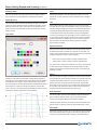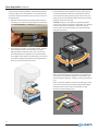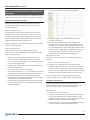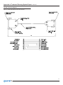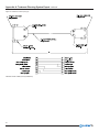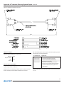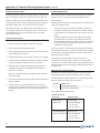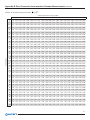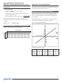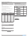
1
WWW. .COM User Manual STANDARD IMAGING, INC. 3120 Deming Way Middleton, WI 53562-1461 Mar / 2012 ©2012 Standard Imaging, Inc. DOC #80614-00 TEL 800.261.4446 TEL 608.831.0025 FAX 608.831.2202 www.standardimaging.com General Precautions Warnings and Cautions alert users to dangerous conditions that can occur if instructions in the manual are not obeyed. Warnings are conditions that can cause injury to the operator, while Cautions can cause damage to the equipment. WARNING: Where applicable, Standard Imaging products are designed to be used with the versions of common radiation delivery devices, treatment planning systems and other common computer software products or systems used in the delivery of ionizing radiation, available at the time the Standard Imaging product is released. Standard Imaging does not assume responsibility, liability and/or warrant against, problems with the use, reliability, safety or effectiveness that arise due to the evolution, updates or changes to these products or systems in the future. It is the responsibility of the customer or user to determine if the Standard Imaging product can be properly used with these products or systems. CAUTION: Do not fill either water tank or reservoir unattended. CAUTION: Water reservoir can be filled using either fill port as they are connected internally. Use caution not to overfill reservoir if using both fill ports. Fill capacity is approximately 60 gallons (265 liters). CAUTION: Do not clean water tank with abrasive cleansers, isopropyl alcohol or other volatile solvents. CAUTION: Do not submerge or scrub the Motion Controller, Electrometer, and Lift and Reservoir Cart in water or solvent to clean. CAUTION: When moving the Lift and Reservoir cart, avoid inclined surfaces. WARNING: Proper use of this device depends on careful reading of all instructions and labels. CAUTION: While in use, place power supplies outside of the Lift and Reservoir Cart storage cavity to prevent overheating. WARNING: An electrical shock hazard of up to ±450 VDC is possible whenever the bias voltage is active. Always set the bias to the 0% or 0 VDC level whenever a device is connected to or disconnected from the electrometer. Do not enable bias on a measurement channel connected to a diode detector. CAUTION: Only push the Lift and Reservoir Cart with the cart handles. WARNING: This equipment is not intended to be used in flammable mixture atmospheres. Do not use with flammable anesthetic mixture with air, with oxygen, or nitrous oxide. WARNING: Electric shock hazard. Do not disassemble or remove covers from equipment. Refer servicing to a qualified individual. WARNING: Electric shock hazard. Turn the Wireless Pendant off before attempting to change the internal batteries. WARNING: Restrain loose clothing or long hair when working near motor and lead screw assemblies. WARNING: Do not place extremities in or near water tank while sample detector carriage is in motion. WARNING: Use only provided power supplies, which include Protek Power, Model PMP150-14, and are identified in the specifications. The use of any power supply other than the UL/TUV recognized power supplies provided with this unit (Protek PMP150-14 or TRUMPower TMP150-24) and using alternatives other than the UL/CSA recognized or European certified power cord can degrade minimum safety. The power replacements from Standard Imaging Inc. are required for compliance with the requirements of IEC 60601-1. WARNING: System is very heavy, especially when filled with water. Handle with care. CAUTION: If setting the up the phantom for performing split field scans such as a half scan of a 40x40 cm field at depth, see “Appendix F: Phantom Placement for Split Fields” on page 68 for required phantom position. Not using this position may compromise system integrity during scanning. CAUTION: When replacing the Wireless Pendant internal batteries, ensure the correct polarity orientation is used. CAUTION: Do not over fill water tank or reservoir. CAUTION: Always use two or more people to place the DoseView 3D frame assembly on and into the water tank. ii CAUTION: Always use two or more people to place the DoseView 3D water phantom onto the Lift and Reservoir Cart. CAUTION: When rotating the water tank upon the Precision Position Platform, ensure the Motion Controller power cable and Precision Position Platform control knobs do not catch on the platform. CAUTION: It is recommended to place the pendant on the treatment couch or elsewhere when scanning takes place. CAUTION: Use only the provided electrometer with the DoseView 3D. Do not use other manufacturer’s electrometers or dosimeters. CAUTION: Input voltage on electrometer’s triaxial connector should be no greater than +5 V or -5 V. CAUTION: Do not drop or mishandle equipment. CAUTION: Do not use handles to lift the Lift and Reservoir Cart. CAUTION: Do not use white ledge on water tank to lift system while tank is full. CAUTION: Damaged or kinked ionization chamber cables or extension cables should not be used. CAUTION: Upon power on, allow for proper warm-up. CAUTION: The electrometer should not be connected to a detector which is used in direct contact with a patient. CAUTION: Connector end of ionization chamber or diode should not be submerged. CAUTION: Do not rotate the water tank while full or when the Lift and Reservoir Cart is at the maximum height position. CAUTION: When rotating the water tank, push the base of the tank rather than the tank top. CAUTION: If this equipment causes interference with other equipment, the user is encouraged to try to correct the interference by the following: • Increase the separation between equipment • Connect the power supply cord into a different grounded AC outlet or into a circuit controlled by a different circuit breaker • Consult Standard Imaging, Inc. Contents ii General Precautions 2 Conventions Used in this Manual 2Overview 2 Theory of Operation 2 Definitions 3 Before Getting Started with Scanning 3 3 5 8 10 Software Installation and Updating Software Configuration and Preferences Hardware Setup and Preparation Verifying System Performance Pre-scan Checklist 10 Scan Acquisition 10 Phase 1 of 3: Setting Up the Phantom in the Treatment Vault 20 Phase 2 of 3: Software Setup with Scan Acquisition Module 31 Auto Acquisition 33 Phase 3 of 3: During the Scan and Completion of Acquisition 34 Finishing Scanning 35 Scan Processing Module 35 36 38 39 File Management and Display Options Scan Processing Tools Relative Dose Conversion Flatness, Symmetry Calculation and Other Tools 40 Table Generation Module 40 Generating Tables 42 Editing, Printing and Exporting Tables 43 Database Management Module 43 43 44 45 Database Structure The Database Management Interface Editing and Managing Data Files Printing and Exporting Data Files 46 Using the DoseView 3D Lift and Reservoir Cart 46 47 47 48 48 Connecting the Power Supply(s) Filling the Reservoir Draining the Reservoir Using the Control Panel Using the Precision Positioning Platform 50 Appendix A: Treatment Planning System Export 50 Varian Eclipse 51 Philips Pinnacle 52 Elekta/CMS Xio 58 Appendix B: Dose Conversion from Ionization Chamber Measurements 58 58 60 60 62 63 64 65 How to Calculate ICRU-35 Radiation Dosimetry Tables for Calculating ICRU-35 Radiation Dosimetry Calculating TG-25 Dose Conversions Tables for Calculating TG-25 Dose Conversion Calculating IAEA TRS-398 Dose Conversions Tables for Calculating IAEA TRS-398 Dose Conversion Calculating TG-51 Dose Conversions Tables for Calculating TG-51 Dose Conversion 65 Appendix C: Scan Calculations 65 Rotational or Diagonal Scan Calculation 66 Default Scan Limit Calculation 66 Scan Ratio Calculation 67 Appendix D: Algorithms 67 Flatness and Symmetry 67 Table Generation Module 68 Appendix E: Troubleshooting / Frequently Asked Questions 68 Appendix F: Phantom Placement for Split Fields 68 Required Setup Position Instructions 69 Parts and Accessories List 70 Description of Symbols 71 Features and Specifications 72Maintenance 72 Return Policy 74 Customer Responsibility 74 Service Policy 74Warranty 49 Engaging/Disengaging the Caster Pedals 49 Using the Firmware Updater 3120 DEMING WAY MIDDLETON, WI 53562-1461 USA WWW.STANDARDIMAGING.COM 1 Conventions Used in this Manual Buttons: When a button is described, it is surrounded by [ ] marks. Example: Press [OK] to proceed. Menu Paths: When a menu path is described, it is shown with a > between each level. Example: Navigate to File > Print to print the currently viewed file. Overview This user manual covers the operation and maintenance of the DoseView 3D water phantom (REF 92260) as well as the DoseView 3D Lift and Reservoir Cart (REF 72260). These two pieces of equipment can be used independently, however many sections of this manual consider usage of them as a set. Whenever practical, alternative scenarios will be presented for users using the DoseView 3D water phantom without the DoseView 3D Lift and Reservoir Cart. Theory of Operation The DoseView 3D is a 3-axis water phantom system designed to acquire and manage beam data accurately, efficiently, and comprehensively from radiotherapy treatment machines such as linear accelerators and cobalt 60 units. Beam data acquired from the DoseView 3D is typically used for three objectives: Acceptance testing and commissioning, quality assurance testing, and clinical reference dosimetry. The system is comprised of several main components as follows: • 3-Axis motion assembly comprised of: DoseView 3D Motion Controller with on-board control panel and wireless radio 5 stepper motors with relative encoder feedback Stainless steel lead screw drive system DoseView 3D Wireless Pendant for motion assembly control and limit setting DoseView 3D Electrometer with 2 channels • Acrylic water tank facilitating scans within a volume of 500 x 500 x 410 mm (Length x Width x Height) • Measurement detectors such as commercially available ion chamber and diode based detectors • Set of measurement detector holders with accompanying water surface setup kit • DoseView 3D Microsoft Windows® based software for coordinating scan acquisition, processing, and an export to one or many TPS (treatment planning systems) • (Optional) DoseView 3D Lift and Reservoir Cart comprised of: DoseView 3D Precision Positioning Platform Motorized lift mechanism Unidirectional motorized pump for active fill and passive drain of water phantom This user manual will provide in-depth instruction covering the procedures and algorithms used in the three main phases of operation: scan 2 acquisition, scan processing and analysis, and export. Furthermore, additional topics and tools will be covered including PDD, TPR and TAR Table Generation, relative dose conversion and database management. Definitions Initialization – Initialization causes the detector to drive to the corner of the phantom nearest the power switch, establishing a home position for the motor encoders. Initialization must be performed each time the phantom is powered on, and resets any origin or soft limits that have been set. Default Origin – The default origin is the point to which the detector travels when the phantom is initialized. This is at the approximate physical center of the X and Y axes, and is roughly the fill point for water in the phantom along the Z axis when using the Lift and Reservoir Cart. Hard Limits – Hard limits are those defined during the initialization process. These are the physical limits to which the detector carriage can travel regardless of detector size. Soft Limits – Soft limits are those optionally defined based on user preference. Soft limits can be configured using the Wireless Pendant or the DoseView 3D software. If a maximum or minimum soft limit is not defined for a given axis, the system will instead respect the hard limit defined during initialization. Detector – A detector is the measurement instrument used with the DoseView 3D. The term detector can be used interchangeably with “probe”. Fast Axis – The fast axis is typically defined as the profile axis. In most scans it is configured to be the X axis to minimize the amount of mass moving quickly through the water during profile acquisition. Slow Axis – The slow axis is typically defined as the axis along which sets of profiles are acquired. Since movement along this axis is typically less frequent, it can be configured for the Y or Z axes without concern for water perturbation. Water Phantom – A water phantom is defined as the complete system of the acrylic water tank, DoseView 3D Motion Controller, movement arms, detector carriage, DoseView 3D Electrometer and Wireless Pendant. Motion Controller – The Motion Controller is the control box which communicates commands to and from the Wireless Pendant, movement arms, DoseView 3D software, and DoseView 3D Electrometer. Wireless Radio – The wireless radio attaches to the PC via an RS-232 serial connection and provides communication to and from the PC and DoseView 3D Motion Controller. Sample Detector – The sample detector is the moving detector mounted on the detector carriage of the DoseView 3D water phantom. Reference Detector – the reference detector is a fixed detector mounted on the reference detector holder of the DoseView 3D water phantom. Definitions continued Before Getting Started with Scanning continued Normalization Point – When normalization is performed, the current detector position is defined as the Normalization Point. This point is saved as a known location and can be returned to using the Move/Set tab within the Scan Acquisition module. When normalization occurs, the measured value will be treated as 100% for the next scan. After completing a set of scans, the detector will return to the normalization point. desktop computer can be used assuming it meets the recommended requirements. A portable notebook computer can be helpful especially if the phantom cannot easily be placed near the computer during initial setup and diagnostics. Before Getting Started with Scanning One or two weeks prior to getting the DoseView 3D into a treatment vault and starting scan acquisition, it is highly recommended to perform some key initial setup and diagnostic procedures to help avoid any delays when it is time to scan. Since in the majority of facilities, a 3D water phantom such as the DoseView 3D is used as infrequently as once per year, verifying system integrity and familiarizing oneself with software operation can help maximize efficiency during limited windows of scanning opportunity. The following sections detail recommended preparation procedures both for first time and for repeat uses of the DoseView 3D: • Software Installation and Updating, including system requirements • Software Configuration and Preferences • Hardware Setup and Preparation • Verifying System Performance • Pre-scan Checklist Software Installation and Updating Included with the DoseView 3D is a CD-ROM for installing the DoseView 3D software on a Microsoft Windows based computer. If the DoseView 3D has recently been purchased, chances are the most recent version is included on the provided CD-ROM, however new updates are periodically released. It is highly recommended to use the latest versions of software available for best performance and functionality. Prior to installation, check with Standard Imaging to get the latest and most up-to-date version of DoseView 3D software and firmware. Prior to installation, verify the computer to be used meets the minimum system requirements for this software. Installation Instructions Before installing the software, it is recommended to close all other active programs. NOTE: The account under which the DoseView 3D software is installed must have at least “Power User” access privileges within Windows. However, the software can be run as a basic “User”. See the system administrator or operating system documentation for assistance and/or further details. 1. Insert the program CD-ROM into the computer’s CD-ROM drive. If autorun is enabled, the installation wizard will begin automatically. 2. If autorun is disabled, browse to the CD-ROM root directory via Windows Explorer and double-click DoseView3DSetup.exe to start the installation program. 3. Read through the software license agreement and click [next] to proceed with the installation. If desired, a DoseView 3D program icon can be placed in the following places: desktop, start menu and quick launch bar. 4. If prompted, restart the computer to complete installation and begin using the DoseView 3D software. When installed, the program will be installed in the “X:\Program Files\ Standard Imaging\DoseView 3D” folder (Program Files (x86) folder for 64-bit Windows installations), where “X” is the system hard drive letter. The default data location is “X:\Documents and Settings\All Users\Documents\ Standard Imaging\DoseView 3D” for Windows XP installations, and “X:\ Users\Public\Standard Imaging\DoseView 3D” for Windows Vista and Windows 7 installations. The default data location can be configured in the DoseView 3D Preferences window. Software Configuration and Preferences Once the DoseView 3D software is installed, a few parameters must be configured to begin using the system. To set these parameters, first launch the DoseView 3D software. From the home screen, navigate to Setup > Preferences to display the preferences window as shown. DoseView 3D Software System Requirements Operating System Microsoft Windows XP SP2 or greater, 32-bit / Windows Vista SP1 or greater, 32-bit / Windows 7, 32-bit and 64-bit versions supported Processor Intel® or AMD®, 350 MHz or greater Memory 512 MB or greater Hard Drive 30 MB or greater Screen Resolution 1024 x 768 or greater CD-ROM Drive 2X speed or greater Connectivity 9-pin, RS-232 serial port or USB port with USB to RS-232 adapter Other Windows versions may also run DoseView 3D software; however they are not officially supported by Standard Imaging. Any notebook or 3 Before Getting Started with Scanning continued Institution Name Units This name will appear in the upper right corner of the software interface and be included on reports generated by the DoseView 3D software. All DoseView 3D distance units will be displayed in either cm or mm as selected. All on-screen indicators as well as generated reports will respect this setting. Default Directory This is the location where DoseView 3D data files are stored. These files include scan results, treatment machine and detector information, and any tables generated by the system. This location can be specified to be any folder for which the current Windows account has write-access, including network locations. Color Setup TPS Some treatment planning systems require direct connection to transfer scan data rather than use of an exported file. If using one of these systems, select the settings that match the port used on the DoseView 3D software computer and configuration required by the treatment planning system’s communication protocol. Only port numbers 1 through 8 are supported, so if using a port higher than 8, select another port or reconfigure the port number assignment within Windows Control Panel. Consult the operating system documentation for additional information. Consult the treatment planning system’s manufacturer for additional information regarding required serial port settings. Hardware Interface Select the communication port settings to match the port used to connect the DoseView 3D Motion Controller to the computer. In most cases, only the port number parameter will need to be changed, however the baud rate is different depending on wired or wireless operation. • Direct cable connection to Motion Controller: 115200 baud rate • Wireless radio connection to Motion Controller: 9600 baud rate Only port numbers 1 through 8 are supported, so if using a port higher than 8, select another port or reconfigure the port number assignment within Windows Control Panel. Consult the operating system documentation for additional information. Motors Clicking the Color Setup button will display a dialog allowing selection of colors appearing on DoseView 3D scan graphs. Background Color dictates the background color of graphs, while Pen Colors and the order in which they are presented on the dialog dictate the color of individual scan profiles as they appear on a graph. For example, if the first four colors are blue, green, cyan and red, the following graph will be displayed. A Pen Color that is the same as the Background Color cannot be selected. The motor min and max speeds correspond to the axis movement speeds of the DoseView 3D. When selecting the speed of any axis within the Scan Acquisition, Axis Definition interface, “Low” will correspond to the “Min speed”, while “High” will correspond to the “Max speed”. E.g. if the Min speed setting is set to 4 mm/Sec, the Low setting within Axis Definition will be 4 mm/Sec. If the middle of the slider is chosen for the axis speed, the midpoint of Min and Max speed parameters will be used. Auto Acquisition The Auto Acquisition function supports multiple configurable lists broken down by treatment planning system. If any of the systems listed are checked, they will appear within the Auto Acquisition interface. The Auto Acquisition Directory is the location where Auto Acquisition Scan Sets are stored. If no directory is selected, the Default Directory is used. Demo Mode Demo Mode provides the ability to use or demonstrate the Scan Acquisition portion of the software while not having the DoseView 3D attached to the computer. This is particularly useful for becoming more familiar with the 4 Before Getting Started with Scanning continued software’s operation or providing training even when the water phantom is not accessible. When not in Demo Mode, if the water phantom cannot be found, the Scan Acquisition portion of the software is inaccessible. When the Demo Mode box is checked, the upper right corner of the software interface will display “DEMO MODE”, and external communication to any attached equipment will be ignored. However, all requirements that are needed while setting up a scan still apply, so initializing and other key steps are needed to proceed with a demo scan. NOTE: In Demo Mode, all hardware communication and beam scanning results are simulated and generated by the software. If a water phantom is attached while using demo mode, it will be ignored and will not move while the demo scan takes place. Hardware Setup and Preparation A few additional steps are needed after uncrating to prepare the DoseView 3D for use. Power Supply and Cable Connection Instructions When Using the DoseView 3D Lift and Reservoir Cart Included with the DoseView 3D and the DoseView 3D Lift and Reservoir Cart are identical power supplies. Both power supplies are attached to the cart with a pass through power cable extending up to the Motion Controller to provide power to the water phantom. When configuring the electrometer settings in Demo Mode, certain settings and orders of operation are required to allow a demo scan to occur. See the applicable sections of this manual to verify how to adjust the following settings. 1. Configure all other scan settings such as Axis Definition and machine selection, and navigate to the Electrometer Setup tab. 2. Set the bias voltage to -300 V for one or both detectors. 3. Click [Zero Electrometer]. 4. Click [Check Max Dose Point]. 5. Click [Set Normalization]. 6. Click [Start Scan]. From here, a mock graph will be plotted based on the selected Axis Definition parameters. 1. On the end of the cart with the taller handle, locate the large sliding door and open it, revealing a storage compartment with two power connectors. 2. Connect a power supply to each port. Since both supplies are the same, it does not matter which port is used with which power supply. 3. Connect the provided wall outlet power cord to each power supply. Comm Log The Comm Log provides a method for seeing internal communication between the electrometer, motion controller and PC over and above what the typical user interface shows. When the Comm Log box is checked, and Scan Acquisition mode is entered, a log display will appear along with the typical interface. This can be useful for troubleshooting in coordination with a Standard Imaging service representative. Log File When the Log File box is checked, a text based log file will be generated documenting everything that would appear in the Comm Log. Log files are generated on a per day basis, so all sessions on a given day will be appended to a single file. These files are stored in the selected Default Directory. Captured Data This function is for Standard Imaging diagnostic work only. 5 Before Getting Started with Scanning continued 4. From the top of the cart, extend the power extension cable to the Motion Controller connector port allowing for adequate slack for when the phantom is rotated. To prevent the rubber grommet from coming loose when pulling the extension cable, hold it down with one hand while pulling the cable with the other. When Using Another Cart 1. Plug the included power supply into the Motion Controller as shown. Use the red alignment dot on both the connector and plug for assistance in orientation. 2. Connect the provided wall outlet power cord to the power supply. Installing the Triaxial Junction Cable Included with the DoseView 3D is a 1 m triaxial junction cable which allows for snag-resistant use of the sample detector within the water phantom. Connect one end to the DoseView 3D Electrometer “Sample Probe” connector and the other end to the triaxial junction point on the opposite side of the phantom. Installing the Reference Detector Holder If using the DoseView 3D to measure a pulsed beam, such as a beam from a linear accelerator, the use of a reference detector is required. The DoseView 3D includes a Reference Detector Positioning Kit containing the following: 5. Connect the cable to the Motion Controller using the red alignment dot on both the connector and plug for assistance in orientation. NOTE: When not in use, the power supplies and power cables can be stored in the cart storage compartment, however to prevent any heat issues, it is recommended to leave the sliding door open while the DoseView 3D is in use. Furthermore, the power supplies can safely be used on the floor to achieve extra cable length if needed. 6 • Base post • Short carbon fiber tube • Long carbon fiber tube • Tube coupler • Reference detector holder • Tube/base post combination fastener The exact combination of components used will vary depending on the field size being measured, however the base post and combination fastener would be installed in any case. On the top of the frame assembly, there are two threaded holes which support the base post. These can be chosen based on the desired detector position; however the hole closest to the electrometer is typically used to minimize cable obstruction. The combination fastener will need to be slid onto the base post before mounting the post onto the frame. Before Getting Started with Scanning continued 3. Tighten the clamp when it is approximately half way along the water tank connection port to seal the tube in place. Filling the Water Reservoir The two included carbon fiber rods can be installed into the combination fastener immediately or set aside for later use. Connecting the Water Tube from the Reservoir to the Water Tank If using the DoseView 3D Lift and Reservoir Cart, the water tube must be connected to the DoseView 3D water tank to perform filling and draining operations using the following steps: 1. Using a slot-head screwdriver, loosen and press a tube clamp over the end of the tube extending from the cart. 2. Press the tube from the cart onto the connection port on the water tank. The end of the tube should be nearly flush with the connection assembly. When using the DoseView 3D Lift and Reservoir Cart, it is a good idea to fill the reservoir in advance of scan acquisition to save time and allow the water temperature to equilibrate with the ambient environment. To maintain the appearance and smooth operation of the plumbing and motion components, it is recommended to use distilled water whenever possible. Avoid using hard water or water with harsh chemical additives to help minimize corrosion and maintain the integrity of the system. Contained in the Lift and Reservoir Cart are two large reservoir tanks, each with a fill port sealed with a screw-on black lid on the top of the cart. Since these two reservoirs are connected internally via plumbing, it is recommended to fill both reservoirs using only one port to prevent overfilling. To fill these reservoirs, use the following steps: Unscrew the two black reservoir lids. One will be used to fill, while the other will be used to verify the water level of the second tank. With a hose, bottle or other method, pour water into the reservoir via either fill port. The second reservoir will fill at a slower rate than the reservoir being actively filled, so attention must be given to prevent overfilling and to ensure both reservoirs are full. It is important to maximize the amount of water in the two reservoirs as this will provide the most available scanning depth when water is transferred to the water phantom. NOTE: While it is not recommended to leave water within the reservoir tanks in-between usages of the cart, unwanted algae and bacterial growth can be addressed with 12-16 oz of hydrogen peroxide per 30 gallons of water. The DoseView 3D Lift and Reservoir Cart holds approximately 60 gallons of water. 7 Before Getting Started with Scanning continued Installing the Communication Cables and Wireless Radio Install Batteries in the Wireless Pendant To communicate with the DoseView 3D via a computer interface, the included serial cable must be routed from the control console into the treatment vault where the DoseView 3D will be used. This cable can be run via the raceway, conduit or maze. In addition, the Xbee radio box must be set up with its included power supply. Last, if needed, a USB to serial adapter should be installed and configured on the host PC. Use a crosshead screw driver to remove the battery door on the back of the wireless pendant, and install four AA batteries in the orientation shown on the rear label of the pendant. Using the power switch located on the right edge of the pendant, turn on the wireless pendant, verifying operation. While a fresh set of the batteries should last several days of continuous use, it is recommended to have an extra set of AA batteries available during a lengthy scanning session to avoid delays during the scanning process. 1. Run the included 9-pin serial cable from the PC into the treatment vault. This is a standard cable, so any existing serial cables can also be used. 2. Connect the Xbee radio box to the vault side of the serial cable. 3. Connect the Xbee power supply to the Xbee radio box. Verifying System Performance Since a system such as the DoseView 3D is used relatively infrequently, it is recommended to verify that the equipment is functioning properly before performing a long series of scans. Below are recommended diagnostic procedures to perform prior to scanning to help ensure time is not wasted due to unexpected issues. Check Power 1. Supply power to all components a. Connect the included power supplies to the DoseView 3D and Lift and Reservoir Cart and connect the power supplies to available wall outlets as described in the previous sections. When connected, the amber LED located near the power switches of both the Motion Controller and Lift and Reservoir Cart should illuminate. 4. (Optional) Mount the Xbee radio box to the wall via the mounting tabs on either side of the unit. 5. (Optional) Install any USB to serial adapter onto the PC where the DoseView 3D software is installed. In most cases, USB to serial adapters require installation of driver software, so it is recommended to have these drivers installed in advance of scanning to help prevent any IT related headaches. Furthermore, as the DoseView 3D software communicates on communication ports 1-8 only, verify the adapter has been configured for a supported port number. Consult the operating system documentation for additional information. 6. Connect the serial cable to the PC, either directly or via any USB adapters used. If it is not desired to use wireless radio communication to the PC, the serial cable can be connected directly to the DoseView 3D Motion Controller as shown. b. Install (4) AA batteries into the Wireless Pendant by removing the pendant’s rear panel with a crosshead screwdriver, and installing the batteries in the orientation indicated on the pendant’s rear label. 2. Verify Water Phantom power a. Power on the DoseView 3D Motion Controller and Electrometer using the switch on the side of the Motion Controller. The green LED adjacent to the amber LED should illuminate indicating system power on. b. Press and briefly hold the [INITIALIZE] button on the Motion Controller control panel until the DoseView 3D arms begin moving the detector carriage to the home position. The carriage should come to a rest near the center of the phantom. 3. Verify Lift and Reservoir Cart power a. Power on the DoseView 3D Lift and Reservoir Cart using the switch on the cart’s control panel. The green LED adjacent to the amber LED should illuminate indicating system power on. b. Use the cart’s on-board control panel to raise and lower the phantom. 4. Verify Wireless Pendant Power a. Power on the DoseView 3D Wireless Pendant using its on-board switch. As the pendant boots, a green communication LED should blink, and after a brief moment the pendant display should illuminate and display the detector carriage’s current coordinates. 8 Before Getting Started with Scanning continued Check Motion and Pendant Function Check Water Flow Integrity 1. Attach the power supply, and power on the water phantom and pendant as described in the previous sections. 1. Move the DoseView 3D to a water accessible area for filling the system. 2. Remove any brackets or alignment tools from the detector carriage. 2. Verify that the petcock valve on the underside of the Lift and Reservoir Cart is tight. This valve is located in the middle of the plumbing junction between the two internal reservoirs. This plumbing junction runs underneath middle of the cart perpendicular to the long axis of the cart itself. 3. Perform water phantom initialization. Press and briefly hold the [INITIALIZE] button on Motion Controller control panel until the DoseView 3D arms begin move the detector carriage to the home position. The carriage should come to a rest near the center of the phantom. 4. On the Wireless Pendant or Motion Controller control panel, use the Probe Control buttons to move the detector carriage. Move to the full extent of each axis individually, and check for any binding or inconsistent movement during travel. Modulate the speed using the [PROBE SPEED] button to try both FAST and SLOW options. The carriage should move freely and consistently within its physical limits. 5. Verify the set origin function by pressing the [ORIGIN] button on the top section of the pendant. The coordinates shown on the pendant display should now be 0.0 for all axes. Move the carriage away from the configured origin and press the [GO TO ORIGIN] button. Verify the system goes to the origin as intended. Check Software Installation and Communication 1. Connect the DoseView 3D Motion Controller to the PC using the desired connection method - wired or wireless - as described in the previous sections. 2. Power on the phantom and perform initialization by pressing and briefly holding the [INITIALIZE] button on Motion Controller control panel. 3. Install the DoseView 3D software as described in previous sections (if needed) and launch the application. 4. Within the Setup > Preferences window, verify that the Hardware Interface settings match the intended port configuration. Typically the default settings are sufficient; however the port number may vary by configuration. The correct port number can be determined by checking within Windows Device Manager, typically within the “Ports (COM & LPT)” section. 5. Also within Preferences, verify that “Demo Mode” is NOT checked. 3. Fill the water reservoir as described in previous sections. 4. If necessary, connect the tube from the Lift and Reservoir Cart to the water phantom as described in previous sections. 5. Inspect the fit and tightness of all plumbing connections from the cart to the phantom. If necessary, adjust positioning of the tube interfaces and use a slot-head screwdriver to tighten all clamps. 6. Ensure the exterior water valve is open. In the open position, the valve handle will be parallel with the direction of water flow. 7. Initiate the auto fill process by pressing the Automatic [FILL] button on the Lift and Reservoir Cart control panel. 8. While fill process is taking place, inspect all plumbing junctions and the seams between the acrylic phantom walls and base for any leaks. 9. When the system has been fully inspected, initiate the auto drain process to return the water to the reservoir. The auto drain process is gravity-driven and will complete more quickly if the water phantom is raised to the maximum lift limit. 10. If not scanning in the near future, empty the reservoir using the procedure outlined in the Finishing Scanning section of this manual at the end of the Scan Acquisition section. Check Electrometer/Detector Performance The DoseView 3D electrometer and any accompanying detectors can be tested to varying degrees depending on whether or not access to the treatment beam is available. Ideally, the system should be tested under beam conditions prior to scanning to ensure full confidence, however performance of the system can still be reasonably verified even if the beam is not available. Using water in the phantom is not needed for this procedure. 6. From the home screen, click the [Scan Acquisition] button. The message “Detecting System Hardware…” will briefly display. If the system is detected and communication is established, no errors will show and the Scan Acquisition interface will appear. 1. Position the system where desired, attach power supplies, power on, initialize the system as described in previous sections. 7. If the Scan Acquisition Wizard is enabled, the initial step will appear. Click [Cancel] to exit the wizard. 3. If using a beam to perform measurements, coarsely position the detectors to ensure adequate signal can be measured. 8. Click the Move/Set tab. If a “Please initialize” error does not appear, communication was successful. 4. Connect the DoseView 3D to the PC as described in previous sections. 9. To verify that control can occur, type in a new coordinate and click the [Move to Coordinate] button. The phantom should move as directed, and the new coordinates should display on the software status bar. 5. Launch the DoseView 3D application, ensure demo mode is disabled and enter the Scan Acquisition module. 2. Install the desired detector(s) to be used and connect to the DoseView 3D electrometer. 6. Navigate to the Electrometer Setup tab. 9 Before Getting Started with Scanning continued 7. If using ion chambers, apply the desired bias voltage. Note: No bias voltage is typically used on a measurement channel connected to a diode detector. After 10-15 seconds the signal levels shown on the status bar should stabilize, though they will not necessarily read 0.00 (units are shown in pC). 8. Perform an electrometer zero by clicking the [Zero Electrometer] button. Once this is completed, the signal levels should be stable and remain very close to 0.00 pC. If readings are stable within ±0.10 pC, then the electrometer and detectors are likely functioning properly. 9. If a beam is available, turn it on at this time. After 2-3 seconds, click the [Set Normalization] button. The range will be checked and normalization will occur. Monitor the ratio % displayed on the status bar. Depending on beam conditions, this number should stay relatively stable. Note that depending on the detectors selected and energy and dose rate settings, the High range may be needed. Switch to the high range as instructed and re-verify operation. Pre-scan Checklist Using the proceeding sections as a guide, consulting the following checklist 1-2 weeks prior to formal scanning can help avoid significant problems or issues during scanning procedures. If problems are discovered or questions arise, there will still be time to consult with Standard Imaging or a qualified distributor for assistance. □ Power connections for the DoseView 3D Water Phantom, Lift and Reservoir Cart and Wireless Pendant have been verified. □ The overall water phantom system movement capabilities have been verified. □ The DoseView 3D software has been installed and configured correctly on the computer to be used for scanning. □ □ □ □ □ Communications between DoseView 3D and the PC have been verified. 10 The seals and plumbing connections have been verified. The electrometer and detector performance have been verified. Desired beam modifiers are ready for use (cones, wedges, etc). (Optional) Auto Acquisition scan sets have been created for the desired scan routines. Scan Acquisition Before proceeding with scan acquisition, it is highly recommended to read the previous section of this manual entitled “Before Getting Started with Scanning”. If the DoseView 3D hardware has been set up, including running any communication cables, and the software is installed, updated and properly configured, read the following sections to learn how to acquire beam scans with the DoseView 3D. Phase 1 of 3: Setting Up the Phantom in the Treatment Vault The following section describes one method for positioning the DoseView 3D water phantom beneath the treatment beam and filling it with water using the Lift and Reservoir Cart. By the end of the section, the DoseView 3D should be precisely positioned such that the sample detector is placed at the water surface in the center of the beam, with the coordinate origin set and the system ready for acquiring scans via the DoseView 3D software. The exact height and rotational position of the phantom will vary depending on many factors such as the source to surface distance (SSD), type of scan desired, and type of treatment machine used; however, the following example will describe how to position the DoseView 3D at 100 cm SSD with the x-axis aligned for cross-plane profile acquisition. The outline on the following section provides a quick reference for the recommended setup procedure for a user who is familiar with the DoseView 3D system and is using the Lift and Reservoir Cart. A more indepth and detailed description of setup is given in the following section. Scan Acquisition continued Water Scanning System Setup - Procedure Outline 1. Wheel water phantom and cart into the treatment vault 2. Rotate phantom to scan position, if necessary 3. Position under gantry using shadow of crosshairs as guide, lock casters a. NOTE: If the DoseView 3D arms are centered in the water tank, they may need to be moved to allow visualization of the crosshairs. See instructions below for plugging in, initializing, and moving the phantom arms. Water Scanning System Setup - Detailed Procedure While the following instructions suggest a procedure for accommodating this task, the order and exact procedure for phantom alignment can vary depending on many factors including environmental conditions and user preference. Use the following guide for DoseView 3D specific functionality, but do not hesitate to modify steps as needed to accommodate site and user specific conditions. 4. Attach power supplies, connect to outlets Some of the following instructions are also covered in the “Before Getting Started with Scanning” section of this manual, so certain steps may have already been completed prior to this section. 5. Power on Motion Controller/Electrometer, Wireless Pendant, perform initialization Part 1: Preparing the Treatment Room a. This step can be performed while filling the phantom if the carriage is already positioned in such a way that it is not interfering with the visualization of the crosshairs. 6. Power on Lift and Reservoir Cart 7. Coarse adjust tank height using room lasers and tank fiducial 8. Align tank crosshairs to light field with Precision Positioning Platform 9. Fill phantom using Auto Fill process 10. While filling: a. Power on phantom components and perform initialization, if necessary b. Install Origin Crosshair Alignment Jig c. Use bubble levels to perform initial leveling d. Prepare detectors in brackets e. Connect to PC and launch software Push the treatment couch out of the area beneath the gantry where the DoseView 3D will be positioned. It is recommended to have at least 1.5 meters of space between the end of the couch and the treatment machine. Keep in mind that rotation of the couch column may be required to provide adequate clearance between the cart and the couch. Ensure that the treatment head is level, such that the beam is directed at the floor. Part 2: Coarse and Fine Positioning the DoseView 3D NOTE: The following instructions assume the DoseView 3D Lift and Reservoir Cart is being used. If using another cart, the steps may vary slightly depending on the functionality of the cart being used. 1. Using the Lift and Reservoir Cart, push the DoseView 3D water phantom under the treatment machine gantry into the approximate position as shown. 11. Fine adjust phantom height and water level a. Submerge x-axis and carriage b. Use floating paper matched with ODI to set water height 12. Close water valve 13. Fine adjust leveling: a. Move carriage to pendant corner, adjust carriage depth to center alignment jig at the surface of the water b. Move carriage to electrometer corner, adjust leveling knob to restore alignment of jig to surface c. Drive across, verify level between both corner knobs d. Drive to center/back near third leveling knob, adjust leveling knob to restore alignment of jig to surface e. Drive to all four corners and verify leveling 14. Move to desired origin, set with pendant a. Use crosshair shadow on top surface of Origin Crosshair Alignment Jig b. Surface depth should still be set from leveling exercise, verify if needed 15. Install detectors, re-verify origin 16. (Optional) Launch software, if necessary a. Choose detectors, set bias, zero electrometer and normalize b. Perform Locate Center routine to check origin 11 Scan Acquisition continued Using the Precision Positioning Platform, rotate the DoseView 3D 90° to the scan position. This is the orientation in which the electrometer and motion controller are located away from the gantry. To rotate, use the following steps: a. Release the coarse rotation latch by pulling the latch downward and rotating 180° clockwise, allowing the phantom to rotate freely. 3. Using the treatment machine light field as a guide, position the cart such that the light field crosshairs line up with the black crosshairs on the bottom of the water phantom. Alignment does not have to be perfect for now as further adjustment will be achieved using precision positioning controls on a future step. CAUTION: If setting the up the phantom for performing split field scans such as a half scan of a 40x40 cm field at depth, see “Appendix F: Phantom Placement for Split Fields” on page 68 for required phantom position. Not using this position may compromise system integrity during scanning. b. Once the phantom is within 10° of the desired position, return the coarse rotation latch back to the lock position, and continue rotating the phantom towards 90° until a “click” is felt. This will mean that the platform has engaged in a pre-set detent position on the platform. Since rotation of the water phantom occurs about the crosshairs, alignment of the phantom to the light field should still be very close to the position set in step 2. NOTE: If the DoseView 3D arms are centered in the water tank, they may need to be moved to allow visualization of the crosshairs. See instructions below for plugging in, initializing, and moving the phantom arms. NOTE: The precision positioning controls have a finite range of travel, so it is best to check that they are initially set approximately halfway between their limits in order to allow easy adjustment in either direction to be performed during setup. 12 Scan Acquisition continued 4. Lock the three casters with black levers on the Lift and Reservoir Cart by pressing down on the levers with a foot or hand to prevent the phantom from moving during the next steps. 5. If using the DoseView 3D Lift and Reservoir Cart, attach the two included power supplies using the following steps: a. On one end of the cart with the taller handle, locate the large sliding door and open it, revealing a storage compartment with two power connectors. b. Connect a power supply to each port. Since both supplies are the same, it does not matter which port is used with which power supply. c. Connect the provided wall outlet power cord to each power supply. e. Verify power is present to the Lift and Reservoir Cart by confirming the amber LED is lit on the control panel. Verify power is present to the DoseView 3D Motion Controller and Electrometer by confirming the amber LED is lit on the side of the Motion Controller. f. If using a cart other than the DoseView 3D Lift and Reservoir Cart, simply connect the single power supply directly to the motion controller. d. From the top of the cart, extend the power extension cable to the Motion Controller connector port allowing for adequate slack for when the phantom is rotated. 6. If desired, the DoseView 3D Electrometer can be operated separate from the main system frame. Detaching the electrometer must be performed when the system power is off, though the power supply can remain connected. To remove the electrometer from the frame: a. Pull and hold the spring pin release located behind the connector end of the electrometer. b. Pull the electrometer parallel with its length until it is free from the frame. c. Use the included short serial cable to reconnect the electrometer to the motion controller. This particular cable, which supplies power and communications, must be used to ensure proper operation of the electrometer. d. Longer triaxial cables will be needed when operating the DoseView 3D Electrometer separate from the system frame. 13 Scan Acquisition continued 7. Power on the DoseView 3D Lift and Reservoir cart using the power switch located on the control panel, and power on the DoseView 3D Motion Controller and Electrometer using the power switch located on the side of the Motion Controller. Verify power is present by confirming the green LED is lit near both switches. 8. Initialize the DoseView 3D. CAUTION: When the DoseView 3D is initialized, the sample detector carriage will first move to the upper corner of the water tank closest to the power switch on the side of the Motion Controller to determine its relative position. Immediately afterwards, the carriage will move to a default point centered in the upper portion of the water tank. Ensure any detectors are removed from the carriage during this step to prevent damage to the detector or water phantom. If already installed, the Origin Crosshair Alignment Jig will not interfere with initialization and can remain installed during this process. To initialize the phantom, press and hold the [INITIALIZE] button on either the Motion Controller control panel or the Wireless Pendant. When the carriage begins to move after a moment, release the button. Until this step is performed, the Detector Control movement buttons are not operational. NOTE: The following instructions assume the DoseView 3D Lift and Reservoir Cart is being used. If another cart is used, the steps may vary slightly depending on the functionality of the cart being used. 9. Using the Lift and Reservoir Cart, lift the phantom such that the scribed line on the front corner of the tank (or the Origin Crosshair Alignment Jig) is roughly aligned at the desired SSD using the room lasers as a guide. This is accomplished using the Lift and Reservoir Cart control panel. 14 Note: Diffraction through the water tank walls can cause laser lines to shift. It is recommended to use the crosshairs and optical distance indicator (ODI) for fine setup adjustment after the water tank has been filled. 10. Once approximate alignment is achieved, using the Motion Controller control panel or the Wireless Pendant, move the carriage away from the default origin such that the shadow does not block the light field from projecting on the crosshairs. 11. If after lifting the cart, the crosshairs on the base of the phantom have deviated from the light field by more than 2 cm, unlock the casters and bring the cart to closer alignment with the light field. If the alignment is already quite close, use the Precision Positioning Platform to fine tune alignment of the phantom to the light field. Three knobs located on the sides of the platform can be used to adjust the X, Y, and rotational alignment. Scan Acquisition continued While the filling process is taking place, the following steps can be started: a. Power on the Motion Controller/Electrometer and perform initialization, if this has not been done already. b. Install the Origin Crosshair Alignment Jig on the sample detector carriage. NOTE: If one or more wheels of the cart are located on the circular floor plate, stepping on the plate or leaning on the cart can cause the water tank to shift slightly. For ease of setup, it is best to avoid these actions if possible. Part 3: Filling the DoseView 3D Water Phantom and Performing Initial Leveling CAUTION: Before proceeding, ensure the proper steps were taken to attach the filling/draining tube from the DoseView 3D water phantom to the DoseView 3D Lift and Reservoir Cart as recommended in the “Before Getting Started with Scanning” section of this manual. Furthermore, the following instructions assume that the reservoir was filled as described the same section. c. Using the three hand screws located on the cast aluminum frame of the DoseView 3D, perform initial leveling of the motion assembly referring to the two bubble levels located on one side of the X-Z axis assembly. 1. Ensure the exterior water valve, in-line with the filling/draining tube, is open. In the open position, the valve handle will be parallel with the length of the valve itself. 2. Start the automatic fill process by pressing the “FILL” button adjacent to the Automatic designation on the Lift and Reservoir Cart control panel. A float switch within the reservoir will stop the filling process automatically. When the automatic fill process is complete, the water level should be close to the scribe mark on the corner of the tank. This also matches the height at which the detector alignment jig stops after initialization of the motion controller. The automatic fill process takes approximately 7-9 minutes. d. Prepare the detectors to be used for scanning. The following diagrams depict Exradin A18 Ion Chambers being prepared. i. Place the desired chamber bracket onto the Sample Detector Centroid Alignment Jig. 15 Scan Acquisition continued ii. Insert the appropriate detector into the jig. 3. Once the auto fill process has been completed, submerge the Origin Crosshair Alignment Jig using the Motion Controller and Wireless Pendant. iii. Place the included build-up cap onto the chamber tip. 4. Using the lift and water level controls, make any necessary final adjustments to align the water surface at the desired height indicated by the ODI. Tip: Use a piece of paper or a paper towel floating on the water surface to enable viewing of the machine crosshairs and ODI. iv. The fiducial line on the cap indicates the centroid position. Adjust the chamber position such that the line on the build-up cap matches with the line on the jig. Once this is completed, the centroid of the chamber’s collecting volume will match with the center of the crosshairs on the Origin Crosshair Alignment Jig. e. If necessary, connect the DoseView 3D system to the PC as described in the “Before Getting Started with Scanning” section of this manual and launch the DoseView 3D software. CAUTION: Once water can no longer be extracted from the Lift and Reservoir Cart using the on-board controls, do not put additional water into the reservoir fill ports. This will prevent overflow when water is returned to the reservoir from the phantom upon completion of scanning. Furthermore, do not fill the water phantom above the white ledge surrounding the phantom with water from an external source. Exceeding this level could cause overflow when water is returned to the reservoir using the manual or automatic draining functions. 5. Close the exterior water valve to prevent any water from flowing back into the Lift and Reservoir Cart. When closed, the valve handle will be perpendicular to the valve itself. 16 Scan Acquisition continued Filling Using a Cart Other than the DoseView 3D Lift and Reservoir Cart 1. Verify the exterior water valve, in-line with the filling/draining tube, is set to the closed position. When closed, the valve handle will be perpendicular to the valve itself. 2. Run a tube from a water source or pour from a vessel to fill the phantom, not exceeding the white ledge surrounding the phantom. Assuming the phantom is at the desired height, fill until the water surface reaches the desired height as indicated by the ODI using the procedure outlined in the previous section. Part 4: Fine System Leveling and Confirming the Origin While the bubble levels mounted to the DoseView 3D provide an accurate indication of system leveling, it is best to fine tune the control arm leveling using the Origin Crosshair Alignment Jig and the surface of the water. The recommended procedure is described below: 3. Use the Wireless Pendant to move the Origin Crosshair Alignment Jig to the rear of the tank, near the third leveling knob. If necessary, use this leveling knob to bring the Origin Crosshair Alignment Jig back to the water surface. If the Wireless Pendant is used to adjust the depth of the probe at this corner of the tank, repeat steps 1 and 2 above. 4. Once completed, drive the probe to all four corners of the water tank and verify the leveling across the entire water surface. 5. If satisfactory leveling is achieved, re-position the Origin Crosshair Alignment Jig to the center of the water tank and fine adjust the x- and y-axis to match the linac crosshairs. The step function is particularly useful for precision positioning as each arrow button press corresponds to a step of 0.1 mm. Switch to the step function by pressing the [PROBE SPEED] button until “STEP” is illuminated. 6. When completed, confirm the initial origin setting by pressing the [ORIGIN] button the Wireless Pendant. A “beep” will sound and the green LED will illuminate indicating the origin has been set. The display coordinates will reset to zero. 1. Using the Wireless Pendant, move the Origin Crosshair Alignment Jig to the corner of the tank closest to the power switch. Verify that the “X” shape at the front of the Origin Crosshair Alignment Jig is still aligned properly with the water surface. If a small discrepancy exists, use the leveling knob at that corner of the tank to adjust the depth of the Origin Crosshair Alignment Jig to bring it back to the water surface. If a large discrepancy exists, the Wireless Pendant can be used to adjust the carriage depth. 2. Once the Origin Crosshair Alignment Jig is again aligned with the water surface, use the Wireless Pendant to move the carriage along the x-axis of the tank to the corner near the electrometer. Again, verify that the “X” shape at the front of the Origin Crosshair Alignment Jig is still aligned properly with the water surface. If a small discrepancy exists, use the leveling knob at that corner of the tank to adjust the depth of the Origin Crosshair Alignment Jig to bring it back to the water surface. If the Wireless Pendant is used to adjust the depth of the probe at this corner of the tank, repeat step 1 above. 17 Scan Acquisition continued Part 5: Installing the Sample Detector Once the motion controller arms are level with the water surface and the origin has been defined, the Origin Crosshair Alignment Jig can be replaced with the desired detector and accompanying bracket. If the detectors to be used are not already installed in their brackets, read the previous section for this procedure. Once installed, the physical center of a cylindrical ion chamber will be placed at the center of the crosshairs on the alignment jig. For most parallel plate ion chambers, the surface of the collecting volume will be placed at the center of the crosshairs on the alignment jig. Once the detector(s) are prepared, follow the instructions below for installation: 1. Remove the Origin Crosshair Alignment Jig by loosening the two thumbscrews and set these components aside. 2. Place the desired detector bracket on the carriage and tighten the two securing thumbscrews. Brackets containing horizontally oriented cylindrical ion chambers such as the Exradin A18 Ion Chamber or parallel plate ion chambers such as Exradin A11 Ion Chamber or the PTW Markus® should be installed on the top of the carriage, in the same place and orientation as the Origin Crosshair Alignment Jig. For vertically oriented detectors, the bracket should be installed on the face of the carriage. 18 NOTE: When a bracket is installed on the face of the carriage, there is a 10.4 mm offset in the -Y direction. For detectors installed using the vertical orientation, apply a Y axis -10.4 mm correction to the origin. Note that this will move the detector 10.4 mm closer to the Motion Controller and Electrometer. 3. If necessary, connect the included 1 m triaxial junction cable from the DoseView 3D Electrometer “Sample Probe” connector to the triaxial junction point. If used, connect the detector’s signal cable to the other end of this triaxial junction point. If not, connect the sample detector connector directly to the “Sample Probe” connector on the electrometer. Scan Acquisition continued Part 6: Defining Positional Limits Depending on the size of the detector used in the carriage, it is recommended to set positional limits to prevent the detector or its signal cable from inadvertently striking the sides of the phantom during scanning procedures. For most detectors, typically only the ±Y axis limits need to be set, however limits can be defined for both directions of all three axes. To define limits, use the following procedure: 1. Using the Motion Controller or Wireless Pendant, move the carriage along any axis to a point which the detector should not travel past. 2. On the Wireless Pendant Limit Settings area, press the button that corresponds to the limit to be defined. The green LED on the button will illuminate, indicating the definition has been made. 3. Continue repeating steps 1 and 2 until all desired limits are defined. Part 7: Installing the Reference Detector and Finish 1. Depending on the field size to be delivered, one or both reference holder tubes may be needed to position the reference probe properly in the field. Prepare tube assembly for installation using the black joiner piece if needed. The image shown in the following step shows only one tube section in use. 2. Loosen the combination fastener and insert the tube into it. 3. If the diameter is sufficient for the detector used (less than or equal to 8 mm such as the Exradin A18 Ion Chamber), slide the detector into the tube and if desired attach the reference detector holder onto the tube assembly. If used, tighten the white thumbscrew to fix the reference detector in place. For larger detectors a small piece of tape can be used to secure the detector in place. 4. Position the reference detector such that the detector’s shadow can be partially seen in the field area. The corner is an ideal spot as it prevents the reference detector from obstructing the measurement path of the sample detector. 4. To disengage any limit, hold its corresponding button until a “beep” is heard. The limit’s green LED should no longer be illuminated indicating the limit is no longer set. 5. To save batteries, turn the Wireless Pendant off. NOTE: All positional and limit information is stored within the Motion Controller so no settings will be compromised by turning off the pendant. However, if the Motion Controller is turned off or unplugged, all settings will be lost and initialization must be repeated. CAUTION: To minimize the Wireless Pendant’s exposure to beam scatter, it is not recommended to place the pendant on the phantom holster during scanning operations. Place the pendant on the treatment couch or elsewhere when scanning takes place. 5. Place the included build-up cap on the reference detector. At this point, the DoseView 3D water phantom should be ready for scanning. 19 Scan Acquisition continued Phase 2 of 3: Software Setup with Scan Acquisition Module This section of the manual covers the Scan Acquisition area of the software which allows for detailed programming of the phantom as well as definition of detectors, machines and energies associated with each scan. The Scan Acquisition module of the software can be operated via two distinct methods. The first method is a step-by-step Scan Acquisition Wizard that breaks down scan setup into easily manageable and explained portions, concluding with the start of scan using the DoseView 3D water phantom. While the wizard is the easiest method for initiating a scan, many advanced scanning options are unavailable and scan setup may take longer overall. Users more comfortable with the software may want to initiate a scan using the second method: the software’s tab interface. This interface contains every scanning option available when using the DoseView 3D, each being accessible at any time. While the tab interface is still quite easy to use, additional explanation may be required which will be covered here in detail. As instruction is already provided on the various Scan Acquisition Wizard steps, this section of the manual will focus on the functions available on each of the Scan Acquisition interface tabs, but will begin briefly with the wizard’s initial steps. Getting Started Before beginning, ensure the DoseView 3D hardware is set up and the origin is defined as outlined in the previous section of this manual, “Phase 1 of 2: Setting up the Phantom in the Treatment Vault”. Exit the vault and go to the computer where DoseView 3D software is installed and configured. 1. Launch the DoseView 3D software. The main screen is displayed with the following options: a. Scan Acquisition b. Scan Processing c. Table Generation d. Database Management e.Exit 2. Click the [Scan Acquisition] button. When Scan Acquisition is launched, the software will poll the serial port for the DoseView 3D hardware. 3. If a DoseView 3D system is not found, an error will occur. This can be caused by several factors which are covered in the “Troubleshooting” section of this manual. 20 4. If a DoseView 3D system is found successfully, the Scan Acquisition Wizard will begin. 5. The first time the Scan Acquisition Wizard is launched, two extra steps will be presented as follows: a. Institution Name - Used on reports generated by DoseView 3D b. Unit Preference - Selectable between mm or cm 6. Once the previous two steps are completed, the typical starting point for the wizard will be selecting the beam type. Proceed with the wizard if desired, otherwise click [Cancel]. From here, the following instructions will cover using the tab interface that is available upon clicking [Cancel]. The Scan Acquisition Tab Interface The Scan Acquisition tab interface is comprised of six tabs as follows: • Initial Setup • Auto Acquisition • Move/Set • Machine Info • Axis Definition • Electrometer Setup The contents of each tab will be explained in order below starting with Initial Setup, except for Auto Acquisition which will be explained last as it encompasses settings from the rest of the tabs. Scan Acquisition continued Initial Setup Beam Type Pulsed mode is for linear accelerator type beams, while Continuous is for active source type beams such as a Cobalt-60 or Cesium-137 irradiator. The difference in scanning operation is that in Pulsed mode, measurements will be based on a ratio between two detectors, a sample and reference detector, while in Continuous mode only the sample detector is used. Selecting Continuous will disable the reference detector in Detector Definition. Detector Definition By default, no detectors are available in the pull-down menus accompanying the Sample and Reference fields. To add a detector, click either [Add] button. A dialog with appear with an opportunity to enter a Detector Description, Detector Inner Diameter and Detector Type. After entering the required information, click [Add] to add this detector to the database. This new entry will now be selectable for both the sample and reference detectors. Continue to add more detectors if desired, and click [Close] when completed. NOTE: Detector inner diameter refers to cylindrical chambers only. For plane-parallel chambers or diode dectectors, enter zero in this field. Once selected, these detectors (or detector for Continuous mode) will be associated with the scan acquired in this session, and will be included in printed reports and exported files. Furthermore, the detector diameter will be used in calculations when converting scan data to relative dose (ion chambers only). Initialize Waterphantom This button performs the same operation as pressing the [INITIALIZATION] button on the Motion Controller or Wireless Pendant: Driving the carriage to the corner of the phantom to determine its position relative to that known point. Typically this function does not need to be performed by the software as it was likely already performed during phantom setup. When navigating away from the System Hardware tab, if the message “Please initialize the waterphantom” appears, the phantom is either not initialized or initialization status cannot be determined due to a communication problem. See the troubleshooting section of this manual for more information. NOTE: Only re-initialize as a last resort to solve motion problems as initialization will discard the origin position and all limit settings. 21 Scan Acquisition continued Orientation Move/Set Tab The Move/Set tab is designed to provide various methods to determine and adjust the sample detector position as well as allow for definition of various important measurement points. The tab interface is broken down into four main areas: 1. Two 2D images depicting the sample detector location within the phantom as shown by a red dot. The exact coordinates of the sample detector can be viewed on the status bar located on the top of the screen. Clicking the button next to Orientation will display a dialog allowing selection between four possible phantom orientations. The thick black bar located on one edge of the phantom in each image represents the DoseView 3D Electrometer and Motion Controller. Click the image that depicts how the phantom is positioned relative to the gantry to establish proper axis definitions. 2. Coordinates, if set, of specific points which can be set by the system: Normalization Point, Max Dose Point, and Origin and how many markers, out of a possible ten. 3. Three buttons across the bottom allowing for the move/set functionality as listed below. 4. Move to Coordinate dialog that allows entry of a specific X, Y, Z coordinate. Clicking [Move to Coordinate] will move the sample detector to the coordinate entered. [Move to Location] Button Options 22 • To Coordinate: Displays a dialog showing the current position and allowing entry of a specific X, Y, Z coordinate. Clicking [OK] will move the sample detector to the entered values. • To Origin: Moves the sample detector to the origin • To Max Dose Point: Moves the sample detector to the max dose point if one is defined • To Normalization Point: Moves the sample detector to the normalization point if one is defined • To Marker: Moves the sample detector to one of ten marker points if any are defined. Marker points can be defined using the Marker interface described in the following manual section, “Set Location”. Scan Acquisition continued [Set Location] Button Options • Limits: Displays an interface which allows the setting of positional limits within the phantom. The limits set using this interface are the same as those set using the Wireless Pendant. To define a minimum or maximum limit for any axis, first move the sample detector to a desired limit position using any available method including the [Move To Location] button or the Move To Coordinate interface. When the sample detector is in the desired position, select an axis, select between Maximum Limit and Minimum Limit and click the [Set] button. [Locate Center] Button The Locate Center function allows the DoseView 3D to measure the location of the center of the radiation field and optionally reset the origin based on the determined position. This function is useful to ensure the DoseView 3D is properly placed for symmetrical scans, and also for determining and quantifying any discrepancies between the radiation field, light field and room lasers. Once the Zero Electrometer, Check Max Dose Point and Set Normalization options have been performed (see the “Electrometer Setup” tab section of this manual for more information), the [Locate Center] button becomes enabled. CAUTION: While software can be used to perform this function, it is highly recommended to set the positional limits in view of the phantom using the Wireless Pendant to prevent any inadvertent detector impacts. The [Reset Limits] button will set all phantom limits to the physical limits of the phantom, also known as the “hard limits”. • Origin: Sets the current sample detector position as the origin • Zero Electrometer: Zeros the electrometer and enables the Set Range/Max Dose Point option • Max Dose Point: Checks if the selected range is adequate for the signal measured. See the “Electrometer Setup” tab for more information. • Normalization: Set the current electrometer reading as 100% dose. See the “Electrometer Setup” tab section of this manual for more information. • Marker: Displays an interface to set up to ten arbitrary marker positions. Before clicking this option, move the sample detector to any position desired to be recalled later. Enter the marker set interface and select any of the ten marker slots. Click the [Set Marker] button, enter a description for the new marker location and click [OK]. From here any marker location can be recalled using the Move to Location, To Marker function described in the previous section of this manual. Click the [Locate Center] button to display the locate center interface. Select an axis to determine a plane for which the center will be located. If the gantry is positioned over the top of the phantom, the Z axis should be selected. If the gantry is aimed at the side of the phantom, select the X or Y axis. This selection will depend on the on the orientation of the water phantom. Enter a depth at which the center of the field will be located and click [OK]. Depending on the axis selected in step 2, a choice of which axis should be centered becomes available. For example, selecting the Z axis in step 2 will allow selection of X, Y, or Both XY. Typically, Both XY is selected to determine the overall center using both directions. Turn the beam on, and click the [Locate Center] button. Locate Center determines the precise central axis position in a plane based on the electrometer readings. 23 Scan Acquisition continued When locating center: 1. DoseView 3D steps in large increments (1 cm) away from the origin in the negative axis direction seeking the location where the reading drops below 50% of the max dose point. 2. Once the under 50% location is found, the detector steps back to the origin in small increments (0.3 mm) seeking the location where the dose reading returns to above 50% of the max dose point and records this point. 3. After the negative axis location is recorded, the same process occurs in the positive axis direction. 4. DoseView 3D then derives the calculated center from the two recorded locations, and compares it to the current origin point. If selected, the system calculates center in this way for both profile axes. 5. If the calculated center is different from the current origin point, DoseView 3D displays the amount of shift required to move the origin point to the actual calculated center. 6. Confirm the shift on either or both axes. NOTE: Locate Center was designed for open field data. The center located on a blocked or wedged field is not the true central ray of the field. Machine Info Tab The following are descriptions of each field available: Scan Description The Scan Description is an arbitrary label that will be saved with the scan and can be edited after scan acquisition occurs. Machine Description By default, only the “Demo Linac” machine is available in the Machine Description pull-down menu. To add another machine, click the [Add] button. A dialog will appear with an opportunity to enter a Machine Description and Source to Axis Distance (SAD). After entering the required information, click [OK] to add this machine to the database. This new entry will now be selectable under the Machine Description pull-down menu. The currently selected machine can be edited by clicking [Edit] and revising either available field. The machine selected here can be changed after scan acquisition occurs. Modality / Energy By default, only “6.00 MV Photon” is available in the Modality / Energy pull-down menu. To add another energy, click the [Add] button. A dialog will appear with an opportunity to enter an energy type and value. After entering the required information, click [OK] to add this machine to the database. This new entry will now be selectable under the Modality / Energy pull-down menu. The energy selected here can be changed after scan acquisition occurs. Dose Rate The Dose Rate can be selected between 100, 200, 300, 400, 500, 600 and >600. In combination with the Modality / Energy selected, the Dose Rate value selected can be used to determine the sampling window of the electrometer during scan acquisition if “Auto Select Based on Dose Rate” is selected on the Electrometer Setup tab. Generally, the higher the dose rate, the smaller the sampling window. Lower dose rates use progressively larger windows to ensure sufficient linac pulses are collected at each point. This value is used only for determining electrometer settings and is not stored within the database after scan acquisition. To recall which dose rate was used after the scan, enter this value into the Scan Description field. The Machine Info tab is designed to provide a method of describing the scan to be acquired in this session. The majority of the fields within this tab are strictly for labeling/categorization and can be changed even after the scan is acquired. However a few fields, such as the Dose Rate and Field Size can have an impact on the performance and options available in other settings. Data in the database are arranged in the following hierarchy: • Machine Description ◦ By default, only “100 cm” (or 1000 mm if units are set to millimeters) is available in the Source to Surface Distance pull-down menu. To add another SSD, click the [Add] button. A dialog will appear with an opportunity to enter a new SSD value. After entering this value, click [OK] to add this SSD to the database. This new entry will now be selectable under the Source to Surface Distance pull-down menu. Modality/Energy Wedge ▪ If a wedge is being used, enter the angle in the Wedge entry field. Use of the arrow buttons will allow entry of any angle from 5 to 95 in 5 degree increments, however any integer from 1 to 99 to can be entered using the keyboard. Source to Surface Distance This means that for each machine entry, several energy entries can exist; for each energy entry, several SSDs can exist. A list of energies and SSDs will need to be created for each machine. 24 Source to Surface Distance Scan Acquisition continued Wedge Description (ISODOSE Only) Fast and Slow Axes If desired, a brief wedge description can be entered in addition to the wedge angle. For example, wedge orientation can be entered in this field Producing any basic or complex profile scan involves programming a plane of motion defined by two axes: the Fast Axis and Slow Axis. Field Size The Fast Axis is the direction along which beam profiles will be acquired, i.e. the direction the sample carriage will move quickly across the field. Generally, the Fast Axis is defined as the X axis, as this axis moves the least amount of mass per step. Orthogonal to the Fast Axis, the Slow Axis defines the positions at which the fast axis scans will be acquired. For instance, to define a series of depths at which to acquire profiles, set the Z axis as the Slow Axis. DoseView 3D supports both symmetric (Square/Rectangular) and asymmetric field sizes. Depending on the Source to Axis Distance (SAD) value set within the machine description and the SSD entered, the Collimator and Surface field sizes can be different. By entering in the desired field size at either Collimator or Surface position, the other will be calculated and filled in automatically. NOTE: The field size does not automatically dictate the scan parameters, and in several cases only acts as a label for the scan. However, if the Fast Axis in the Axis Definition tab (see following section) is set to be configured as “Use Fanline File” or “Use Defaults”, the field size entered here will be used to calculate scan parameters. In these cases, field size entries on the Console tab cannot be modified after the scan has taken place. Clicking on the Fast Axis […] button will display the following options: Axis Definition Tab The Axis Definition tab is used to program the motion routine used by the phantom during scan acquisition. Two scan types are available: ISODOSE and Flatness/QA Check, each with slightly varying options. ISODOSE is used to acquire beam profiles and depth dose curves, while Flatness/QA Check is used to check beam flatness and symmetry at various depths. • Axis – Select the axis to define as the Fast Axis. If only a depth dose measurement is desired, select No Axis. Note that No Axis will also need to be selected for the Slow Axis. • Scan Limits ◦ Use Max Symm Limits – The start and stop values for the Fast Axis will be bound by the maximum symmetrical positional limits set for the phantom. For example, if limits define there to be 15 cm of available travel in the positive direction from the origin, and 13 cm in the negative direction, the Max Symm Limits will define the start and stop point to be 13 and -13 cm respectively. Enter in a step interval to complete the definition. ◦ Use Max Limits – The start and stop values for the Fast Axis will be bound by the overall maximum positional limits set for the phantom, regardless of whether or not these values are equal. Enter in a step interval to complete the definition. ◦ User Specified Points – The start and stop values can be defined arbitrarily regardless of the field size selected on the Console tab, however they must still be defined within the positional limits of the phantom. Enter in a step interval to complete the definition. ◦ Use Defaults – The start and stop values will be defined by the product of two variables: the field width set on the Console tab and the OverScan Ratio setting. For example, if the field is set to 10 cm wide and the over scan ratio is set to 1.4, the resulting overall width would be 14 cm. This would be displayed in terms of the start and stop values as 7 and -7 cm or an overall distance of 14 cm. Enter in a step interval to complete the definition. 25 Scan Acquisition continued ◦ Use Fanline File – The start, stop and step values will be defined by two variables: the field size set on the Console tab and the selected/created fanline file. A fanline file allows data points to be defined in non-equal distances, meaning more points can be acquired in one area of the profile than another. For example, this is helpful to allow more points to be acquired in the high gradient penumbra region than in the central portion of the field, saving time while still gaining detailed data from important areas. If it is desired to put more points around the field edge, insert more points close to 1.000. Points can be inserted between existing rows using the [Insert] button. Note that points can be used in excess of 1.000 as well, up to 3.000 or 300% of the field size. See the following example: A fanline file can be created in two different ways, either prior to a scan in tabular format or during scan acquisition by manually selecting points on the graph. Both methods result in a saved file which can be used in subsequent scan acquisitions. Because fanline files are developed from relative values as opposed to absolute positions, they can be applied to any field size once created. The following procedure covers creating a fanfile file in tabular format prior to scan acquisition. Values Acquisition Location for a 10 x 10 field (not shown in software) 1 3.000 15.00 cm 2 2.000 10.00 cm 3 1.004 5.02 cm 4 1.000 5.00 cm 5 0.996 4.98 cm 6 0.500 2.50 cm 7 0.100 0.50 cm Add any other desired points to the fanline file. Up to 64 1. Click [New Fanline File] on the Fast Axis Definition window. The Edit/Add Fanline File window will display. individual points can be added in total. 4. Upon confirmation with the [OK] button, the values will be arranged in sequential order. Clicking [OK] will add this new file to the Fanline File pull down menu, and the file will be selectable for all future acquisitions. Because the start, stop and step values are all determined by the fanline file and field size, these fields cannot be modified once a fanline file is selected. 5. By default, this fanline definition will be applied to both sides of the field. To apply the fanline file only to the positive or negative side of the field, select the fanline file from the menu, by-pass the edit inquiry, and select the desired side from the side selection window. • 2. Enter a description for the new fanline file. 3. Enter relative position values in the table. These values correspond to a percentage position for one half of the field width. For example, a value of 1.000 will correspond to the 100% position of the field edge. In the case of a 10 cm field width (which would translate to -5 and 5 start and stop values respectively), a value of 1.000 in the fanline table would correspond to an acquisition at 5 cm. Taking it further, adding 0.500 to the table would put another point at 2.5 cm, and adding 0.100 would put yet another point at 0.5 cm. 26 Values Acquisition Location for a 10 x 10 field (not shown in software) 1 1.000 5.0 cm 2 0.500 2.5 cm 3 0.100 0.5 cm Speed – Select the speed at which the selected axis will move from point to point. The definitions for the Low to High can be adjusted in the Preferences window, accessible from the home screen. Scan Acquisition continued ◦ Clicking on the Slow Axis […] button will display the following options: Use Depth File – The start, stop and step values will be defined by the selected/created depth file. A depth file allows data points to be defined in non-equal distances, allowing profiles to be acquired from an arbitrary list of depths. Once a depth file is created, it can be applied to any future scan acquisition. The following procedure covers creating a depth file. 1. Click [Add Depth File] on the Slow Axis Definition window. The Edit/Add Depth File window will display. • Axis – Select the axis to define as the Slow Axis. If only a depth dose measurement is desired, select No Axis. Note that No Axis will also need to be selected for the Fast Axis. • Scan Limits ◦ Use Max Symm Limits – The start and stop values for the Slow Axis will be bound by the maximum symmetrical positional limits set for the phantom. For example, if limits define there to be 15 cm of available travel in the positive direction from the origin, and 13 cm in the negative direction, the Max Symm Limits will define the start and stop point to be 13 and -13 cm respectively. Enter in a step interval to complete the definition. ◦ Use Max Limits – The start and stop values for the Slow Axis will be bound by the overall maximum positional limits set for the phantom, regardless of whether or not these values are equal. Enter in a step interval to complete the definition. ◦ User Specified Points – The start and stop values can be defined arbitrarily regardless of the field size selected on the Console tab, however they must still be defined within the positional limits of the phantom. Enter in a step interval to complete the definition. ◦ Use Defaults – (Unavailable if the Y axis is the fast axis, or if the Z axis is selected as the slow axis) The start and stop values will be defined by the product of two variables: the field width set on the Console tab and the OverScan Ratio setting. For example, if the field is set to 10 cm wide and the over scan ratio is set to 1.4, the resulting overall scan width would be 14 cm. This is displayed in terms of the start and stop values as 7 and -7 cm. Enter in a step interval to complete the definition. 2. Enter a description for the new depth file. 3. Enter the desired scanning depth values into the table. Up to 64 individual depths can be added in total. 4. Clicking [OK] will add this new file to the Depth File pull down menu, and the file will be selectable for all future acquisitions. Because the start, stop and step values are all determined by the depth file, these fields cannot be modified once a depth file is selected. NOTE: Any depth file created can be used for either the Slow or Depth Dose Axes. • Speed – Select the speed at which the selected axis will move from point to point. The definitions for the Low to High can be adjusted in the Preferences window, accessible from the home screen. 27 Scan Acquisition continued (ISODOSE or Flatness/QA Check) Depth Dose Axis 1. Click [Add Depth File] on the Depth Dose Axis Definition window. The Edit/Add Depth File window will display. Use of the Depth Dose Axis allows a depth dose scan to be acquired at the same time as a profile scan. A depth dose scan can also be acquired at the same time as a Flatness/QA Check scan. Setup of the Depth Dose Axis is identical to that for the Slow Axis, however the measurement points are independent of those chosen in the Fast and Slow Axis dialogs. Clicking on the Depth Dose Axis […] button will display the following options: 2. Enter a description for the new depth file. 3. Enter the desired position values into the table. Up to 64 individual positions can be added in total. • Axis – Select the axis to define as the Depth Dose Axis. • Scan Limits ◦ Use Max Symm Limits – The start and stop values for the Depth Dose Axis will be bound by the maximum symmetrical positional limits set for the phantom. For example, if limits define there to be 15 cm of available travel in the positive direction from the origin, and 13 cm in the negative direction, the Max Symm Limits will define the start and stop point to be 13 and -13 cm respectively. Enter in a step interval to complete the definition. ◦ Use Max Limits – The start and stop values for the Depth Dose Axis will be bound by the overall maximum positional limits set for the phantom, regardless of whether or not these values are equal. Enter in a step interval to complete the definition. ◦ User Specified Points – The start and stop values can be defined arbitrarily regardless of the field size selected on the Console tab, however they must still be defined within the positional limits of the phantom. Enter in a step interval to complete the definition. ◦ Use Defaults – Unavailable for the Depth Dose Axis. ◦ Use Depth File – The start, stop and step values will be defined by the selected/created depth file. A depth file allows data points to be defined in non-equal distances. Once a depth file is created, it can be applied to any future scan acquisition. The following procedure covers creating a depth file. 4. Clicking [OK] will add this new file to the Depth File pull down menu, and the file will be selectable for all future acquisitions. Because the start, stop and step values are all determined by the depth file, these fields cannot be modified once a depth file is selected. NOTE: Any depth file created can be used for either the Slow Axis or the Depth Dose Axis. • Speed – Select the speed at which the selected axis will move from point to point. The definitions for the Low to High can be adjusted in the Preferences window, accessible from the home screen. (ISODOSE Only) Off Axis Shift The Off Axis Shift function can be used for acquiring profiles and depth dose curves off of the central axis. Select the desired axis for the shift along with a distance, in positive or negative values. Note that the shift axis cannot also be selected as the Fast, Slow or Depth Dose Axis. For example, with the fast axis set to X, the slow axis set to Z, and the depth dose axis set to Z, an Off Axis Shift is allowed along the Y axis. (ISODOSE Only) Axis of Rotation The Axis of Rotation function allows rotation of the acquisition plane about either the Fast or Slow Axis. Select the desired axis of rotation along with an angle from 45 to -45°. For angles above ±45°, switch the fast axis from X to Y (or Y to X) to rotate about the Z (slow) axis from the opposite direction. NOTE: The Axis of Rotation function will not rotate the phantom, but rather scan at an angle in the phantom using motion along multiple axes. For example, if the Fast Axis is selected as X and the Axis of Rotation is set to Z, the phantom will use combined X and Y motion to generate scan profiles. 28 Scan Acquisition continued (Flatness/QA Check Only) Cross Plane and In Plane Axes Operations for selecting the Cross Plane and In Plane Axes are identical as described below: Clicking on the Cross Plane Axis […] or In Plane Axis […] button will display the following options: ◦ Use Fanline File: The start, stop and step values will be defined by two variables: the field size set on the Console tab and the selected/created fanline file. A fanline file allows data points to be defined in non-equal distances, meaning more points can be acquired in one area of the profile than another. For example, this is helpful to allow more points to be acquired in the high gradient penumbra region than in the central portion of the field, saving time while still gaining detailed data from important areas. A fanline file can be created in two different ways, either prior to a scan in tabular format or during scan acquisition by manually selecting points on the graph. Both methods result in a saved file which can be used in subsequent scan acquisitions. Because fanline files are developed from relative values as opposed to absolute positions, they can be applied to any field size once created. The following procedure covers creating a fanfile file in tabular format prior to scan acquisition. 1. Click [New Fanline File] on the Cross Plane or In Plane Axis Definition window. The Edit/Add Fanline File window will display. • Axis: Select the axis to define as the Cross Plane/In Plane Axis. • Scan Limits ◦ Use Max Symm Limits: The start and stop values for the Cross Plane or In Plane Axis will be bound by the maximum symmetrical positional limits set for the phantom. For example, if limits define there to be 15 cm of available travel in the positive direction from the origin, and 13 cm in the negative direction, the Max Symm Limits will define the start and stop points to be 13 and -13 cm respectively. Enter in a step interval to complete the definition. ◦ Use Max Limits: The start and stop values for the Cross Plane or In Plane Axis will be bound by the overall maximum positional limits set for the phantom, regardless of whether or not these values are equal. Enter in a step interval to complete the definition. ◦ User Specified Points: The start and stop values can be defined arbitrarily regardless of the field size selected on the Console tab, however they must still be defined within the positional limits of the phantom. Enter in a step interval to complete the definition. ◦ Use Defaults: The start and stop values will be defined by the product of two variables: the field width set on the Console tab and the OverScan Ratio setting. For example, if the field is set to 10 cm wide and the over scan ratio is set to 1.4, the resulting overall width would be 14 cm. This would be displayed in terms of the start and stop values as 7 and -7 cm or an overall distance of 14 cm. Enter in a step interval to complete the definition. 2. Enter a description for the new fanline file. 3. Enter relative position values in the table. These values correspond to a percentage position for one half of the field width. For example, a value of 1.000 will correspond to the 100% position of the field edge. In the case of a 10 cm field width (which would translate to -5 and 5 start and stop values respectively), a value of 1.000 in the fanline table would correspond to an acquisition at 5 cm. Taking it further, adding 0.500 to the table would put another point at 2.5 cm, and adding 0.100 would put yet another point at 0.5 cm. Values Acquisition Location for a 10 x 10 field (not shown in software) 1 1.000 5.0 cm 2 0.500 2.5 cm 3 0.100 0.5 cm 29 Scan Acquisition continued If it is desired to put more points around the field edge, insert more points close 1.000. Points can be inserted between existing rows using the [Insert] button. Note that points can be used in excess of 1.000 as well, up to 3.000 or 300% of the field size. See the following example: Values Acquisition Location for a 10 x 10 field (not shown in software) 1 3.000 15.00 cm 2 2.000 10.00 cm 3 1.004 5.02 cm 4 1.000 5.00 cm 5 0.996 4.98 cm 6 0.500 2.50 cm 7 0.100 0.50 cm Electrometer Setup Tab Add any other desired points to the fanline file. Up to 64 individual points can be added in total. 4. Upon confirmation with the [OK] button, the values will be arranged in sequential order. Clicking [OK] will add this new file to the Fanline File pull down menu, and the file will be selectable for all future acquisitions. Because the start, stop and step values are all determined by the fanline file and field size, these fields cannot be modified once a fanline file is selected. 5. By default, this fanline definition will be applied to both sides of the field. To apply the fanline file only to the positive or negative side of the field, select the fanline file from the menu, by-pass the edit inquiry, and select the desired side from the side selection window. (Flatness/QA Check Only) Scan Depth The Scan Depth Function can be used to create a shift when performing a Flatness/QA Check scan. Select the desired axis for the shift along with a distance, in positive or negative values. Note that this axis cannot also be selected as either the Cross Plane or In Plane Axis. The Electrometer Setup tab is used to perform electrometer specific operations, configure final settings and initiate the start of scan acquisition. Electrometer Range By default, the electrometer range is set to Low. The low range provides the best performance for most ion chamber measurements, however when using diodes with higher dose rate beams, the high range may be required. It is recommended to leave this setting as low, and any saturation issues will be identified when the normalization point is set. Note that if the range is changed, a 30 second wait period required before the electrometer can be zeroed. This is to ensure the system has stabilized sufficiently following the range change. Zero Electrometer Clicking the [Zero Electrometer] button will initiate a zero operation on all electrometer ranges. If using ion chambers, it is recommended to zero after the bias voltage has been enabled and has been given a few moments to equilibrate. Check Max Dose Point Clicking the [Check Max Dose Point] button evaluates whether the selected range is adequate for the signal to be measured. Position the sample detector at dmax for non-wedge fields, at the toe of the wedge for wedge fields. If the selected range is determined to be inadequate, try the High range and/or adjust the detector setup. NOTE: The beam must be on to perform this step. 30 Scan Acquisition continued Set Normalization Clicking the [Set Normalization] button will check for electrometer range saturation and define the current signal level at 100% dose when the scan is plotted on a graph. While an initial normalization value must be defined before the start of a scan, this value can be changed after scanning is accomplished, so determining the perfect spot is not critical at this step. Note that measurements can occur above this threshold and will be graphed as values larger than 100%. Before clicking this button, the following steps must be performed for the operation to complete successfully: 1. Position the sample detector at the location where the signal is expected to be roughly at its largest value. In most cases, the center of the field at dmax is an ideal position. Moving the sample detector can be accomplished by using one of several methods on the Move/ Set tab. See the “Move/Set Tab” section of this manual for more information. Auto Acquisition The Auto Acquisition tab, located in the Scan Acquisition module, allows pre-programming of a queue of scans to save time during scan acquisition. The following sections describe how to create and edit Scan Sets prior to and during scanning. Creating a New Scan Set Navigate to the Auto Acquisition tab within the Scan Acquisition module. If the water phantom is not attached the PC, ensure Demo Mode is enabled using the preferences area to access to this function without communication to the phantom. NOTE: Scan sets created in demo mode are available even outside of demo mode. 2. Turn the beam on using the desired energy and dose rate, if applicable. Scan sets are organized as either QA or Commissioning sets within a treatment planning system or under the Custom Scan Sets area on the Auto Acquisition tab. The ability to have scan sets organized by TPS allows creation of a list of scans required by each TPS supported by DoseView 3D. 3. Click the [Set Normalization] button. The current measured value will be treated as 100% when the scan is plotted. To create a scan set, use the following procedure: Electrometer Bias Voltage CAUTION: If using a diode detector, do NOT enable bias voltage as it may permanently damage the detector. For ion chambers, select the desired electrometer bias voltage by choosing a value from the Set Volts pull down menu. To enable the selected voltage to either channel, click the [Off] button next to the desired channel. The Measured fields indicate the voltage currently being applied to each channel. Upon enabling bias, the field will show with a yellow background the value is within tolerance. Start Scan Clicking the [Start Scan] button will begin scan acquisition using the settings selected throughout the tab interface. If some of the settings are invalid, a window will appear listing which settings are incorrect and need to be changed. Note that some of the messages on this window are not requirements but simply notifications. Address any incorrectly specified parameters and click [Start Scan] to begin scan acquisition. 1. Click either QA or Commissioning under either a specific TPS or Customer Scan Sets. 2. Click the [Add New Scan Set] button to add a “New Scan Set” to the list. This name can be changed by selecting the scan set name and clicking the [Rename Selected] button. 3. To view or edit this scan set, either double-click the name or click the [View/Edit Selected] button. The Add/Edit Acquisition File window will display. This screen will eventually show a list of all unique scan definitions that are part of this scan set. 4. Click the [Add New] button to add a new scan definition. 5. To customize the new definition, double-click the name or click the [Edit] button. A window will display that shows the Console and Axis Definition tabs. These tabs are identical to those that are part of the typical scan acquisition interface. 6. Enter in all desired parameters on these tabs as described in their respective sections of this manual. The “Active” checkbox in the lower left corner of the window indicates whether the scan should be active during the scan set. Click [OK] to proceed. 7. Continue to add any more desired scan definitions to the scan set. Add a Helpful Message Prior to the Start of Each Scan Definition It can be helpful to add a reminder message to the start of each scan definition to remind the user of special conditions or set up parameters. Some examples include “Put on 10x10 cm electron cone” or “Rotate water phantom 45 degrees”. To add a message to a scan definition, select the scan and click the [Add/Edit Dialog] button. Enter in the desired message and click [OK] to save/attach this message to the scan. A different message can be applied to each scan within a scan set. 31 Scan Acquisition continued Reordering Scans within a Scan Set Editing a Scan Definition While in the Auto Acquisition Process To adjust the order in which scans will be acquired in a given scan set, select a scan definition and click the up and down arrow buttons located below the [Delete] button. It is possible to make changes to scan definition while in the middle of an auto acquisition routine. On any Setup Instructions window, click the [Edit] button to modify the currently displayed scan definition. The Console and Axis Definition tabs will be displayed. Make any desired changes, and click [Save] to modify the scan set permanently, or [Update] to make this change only temporarily for the current acquisition. Copying a Scan Definition Click any scan on the scan set list and click the [Copy] button to duplicate it. This can be especially useful when creating many similar scans with only minor tweaks. Create a baseline version, make a copy and edit from there to generate a full list of scans quickly. Deleting a Scan Definition Click any scan on the scan set list and click the [Delete] button to remove it from the list. Acquiring Scans with an Auto Acquisition Scan Set A created scan set must first be activated before it can be used. Use the following procedure for activating a scan set and using it to perform a series of scan acquisitions. Managing Auto Acquisition Files From the main Auto Acquisition tab interface, a scan set can be copied, deleted, imported and exported. Copying a Scan Set Select the desired scan set and click the [Copy] button. The selected scan set will be duplicated within the same scan set category. Deleting a Scan Set Select the desired scan set and click the [Delete] button. The selected scan set will be deleted from the scan set category when confirmed with [Yes]. 1. Click the desired scan set from the Auto Acquisition tab. Importing a Scan Set 2. Click the [Activate Selected] button. The Console and Axis Definition tabs will disappear from the Scan Acquisition tab interface as the settings within are now dictated by the scan definitions within the active scan set. Also, the auto acquisition “A” icon shown on the right end of the toolbar will appear as dark green. Select the desired destination scan set category, and click the [Import Scan Set] button to browse for a scan set to import. The selected file will be placed in the scan set category previously highlighted. 3. Proceed to the Move/Set and Electrometer Setup tabs to configure bias voltage, range and normalization settings. Click the [Start Scan] button on the Electrometer to begin the auto acquisition routine. Select the desired scan set, and click the [Export Scan Set] button to browse for an export destination. Choose the desired location and click [Save] to complete the export operation. 4. The Setup Instructions window showing parameters and message configured for the first scan within the scan set will be displayed. Make any necessary electrometer adjustments and click [Scan] to acquire this scan, or click [Next] to skip to the next scan. 5. The scan will be acquired just as during a typical scan process. Once completed the scan can be saved by navigating to Auto Acquisition > Save Current Scan (or Save Current Scan and Continue). The scan can also be edited, retried or skipped using the other available options from the Auto Acquisition menu. Auto Acquisition can be quit by selecting Exit Auto Acquisition. 6. If continuing, the Setup Instructions window for the next scan in the set will be displayed. Make any necessary electrometer adjustments and click [Scan] to acquire this scan, [Next] to skip to the next scan or [Previous] to return to a previous scan. 7. Continue with all available scans until auto acquisition is completed or click [Cancel] from any Setup Instructions window to quit auto acquisition mode. 32 Exporting a Scan Set Scan Acquisition continued Phase 3 of 3: During the Scan and Completion of Acquisition 8. Once the desired points are marked, click the [Quit] button. This section of the manual covers what options are available while a scan is taking place, and how to save a scan file once acquisition is completed. Operations Available During a Scan While the scan is taking place, there are several operations that can be performed. Also, checks have been set in place to ensure a scan completes successfully. Pausing or Aborting a Scan An in-progress scan can be paused or aborted at any time. Click the [Pause] button to pause the scan in progress. Pausing a scan is useful for editing fanline file definition without restarting a scan or returning to the scan acquisition interface. Read the following sections to learn about making these adjustments while a scan takes place. Clicking the [Abort] button will cancel the current scan and return operation to the scan acquisition interface. Defining a New Fanline File While a fanline file can be defined in tabular format prior to scan acquisition, one can also be defined while a scan acquisition takes place using the following procedure: 1. Start a scan using a set step distance, ideally one that is small enough to support the highest density desired for a given profile. 2. Once the scan has completed at least ½ of a profile distance, pause the scan using the [Pause] button. 3. Navigate to Scan > Define Fanline File. The Edit Fanfile File options will become available for use. 4. Use the mouse to click on the in-progress profile. 5. Tap the keyboard arrow keys (<- or ->) to step between each acquired point. Navigate to a point desired to be defined within a fanline file. 6. Click the [Glue] button or press “G” on the keyboard to mark the selected point. The point will now be marked with a red dot to indicate that it will be part of a new fanline file definition. 7. Continue marking the desired points using the method in steps 5 and 6. Click the [Pick] button or press “I” on the keyboard to unmark any previously marked point. 9. A prompt will appear to enter a fanline file description. Enter a description and click [OK]. 10. Another prompt will appear inquiring whether to apply the new fanline file to the current scan. Click [Yes] or [No] to proceed. If yes is selected, the scan will restart using the newly defined fanline file once the [Resume] button is clicked. Clicking [No] will exit the fanline definition interface, and [Resume] can be clicked to resume the scan using the existing fixed step settings. For future scans, this new fanline file will be accessible within the Axis Definition tab. Adjust Graph Axis Scale During a scan, the scale of the graph can be edited using the following procedure: 1. Pause the scan using the [Pause] button. 2. Navigate to Scan > Edit Display Param > Keyboard Limit Set. 3. A window will appear allowing entry of new X and Y axis limits. Enter the desired values and click [OK] to confirm and rescale the graph or [Cancel] to return to the graph screen using the original values. Hitting [Restore] will change any modified entries to their original values. To restore the graph scale to its original limits after new entries are confirmed, navigate to Scan > Edit Display Param > Reset to Default. Completion of Acquisition When a scan is completed, the screen will transition to the Scan Processing interface, covered in detail in the following section of this manual. At this point, the scan can be saved to the database. Saving a Scan File 1. Navigate to File > Save Scan File As… 2. The Console window will appear containing the scan details entered on the Console Tab within the Scan Acquisition interface. Confirm all details are correct or make any necessary changes. Note that if a fanline file was used, the field size cannot be changed. 3. Click the [Save] button to save this scan to the database or [Cancel] to return to the Scan Processing interface without saving. 33 Scan Acquisition continued Finishing Scanning Drain the Water Phantom Turn Off Electrometer Bias Voltage Drain from Phantom to Reservoir Before disconnecting ion chambers from the DoseView 3D Electrometer, be sure to turn bias voltage off using one of the two following methods to prevent shock and potential damage to the electrometer and/or detectors. Using the DoseView 3D Software 1. Navigate to the Electrometer Setup tab with the Scan Acquisition module. 2. Click the [ON] buttons located in the Bias section and the bias voltage will be disabled. 3. Before disconnecting the detectors, verify the bias enabled lights are not lit on the electrometer. Using the DoseView 3D Hardware 1. On either the DoseView 3D Motion Controller control panel or the Wireless Pendant, press and hold the [DISABLE BIAS VOLTAGE] button. 2. Before disconnecting the detectors, verify the bias enabled lights are not lit on the electrometer. 1. Ensure the exterior water valve is open. In the open position, the valve handle will be parallel with the direction of water flow. 2. Press the Automatic [Drain] button on the DoseView 3D Lift and Reservoir Cart to gravity drain the phantom. After approximately 20 minutes the auto process will complete and a small amount of water will remain in the phantom. The remaining water can be absorbed with a towel or left to evaporate. Drain the Reservoir 1. Drain the majority of the water from the DoseView 3D Lift and Reservoir Cart a. Move the cart to a location where the water can be disposed of such as a sink or floor drain. b. Ensure the exterior water valve is open. In the open position, the valve handle will be parallel with the direction of water flow. c. Disconnect the water hose from the DoseView 3D water tank by first loosening the clamp closest to the tank with a slot-head screwdriver and then pulling the tube from the connection port. Use caution to prevent spillage if any water still remains in the tube from the draining process. d. Place the tube end near the water destination (sink, drain, etc) and press the Automatic [Fill] button on the cart’s control panel. This will push the water out until the float switch in the bottom of the reservoir is tripped. 2. Drain the remaining water from the DoseView 3D Lift and Reservoir Cart a. Position the center of the cart over a drain or a surface that will direct the water to an acceptable disposal location. b. Locate petcock valve on the underside of the cart. This valve is located in the middle of the plumbing junction between the two internal reservoirs. This pumping junction runs underneath the middle of the cart perpendicular to the length of the cart. c. Loosen the petcock valve with a wrench or pliers by turning it counterclockwise, and spin the valve cover until it comes free from the system. The remaining water will pour from the reservoir. d. When the water has fully drained, replace the petcock valve cover and ensure it is tight to prevent leakage from the reservoir. 34 Scan Processing Module Adjusting the Scan Display When a scan file is first opened, the Profile View (if available) is shown at the default zoom level encompassing all acquired data points. Individual points can be selected and identified, the graph scale can be changed and the view can be toggled between Profile, CAX and Isodose Views. Raw and Processed View can also be toggled. Selecting and Viewing Individual Profiles and Points Once a scan has been acquired, the Scan Processing module can be used to make adjustments to scan files, convert to relative dose using one of several available protocols as well as calculate some scan attributes such as flatness and symmetry. An individual scan file contains raw AND processed versions of profiles and/or CAX data. No matter what processing is performed to a scan file, the raw version is always preserved within the file. The following sections describe how to use each function within Scan Processing. File Management and Display Options Opening a Scan File Immediately after a scan is completed, the interface automatically switches from Scan Acquisition to the Scan Processing module. Scan Processing can also be accessed from the home screen by clicking the [Scan Processing] button. When the Scan Processing module is launched, a window will display to select an existing scan file organized in the Machine, Energy, SSD hierarchy. Select the desired file and click [OK]. Saving a Scan File Clicking the icon or navigating to File > Save Scan File, will save any changes made to the scan file. Any changes will be stored as the processed version while the raw version will always be left unchanged. To save a new copy of an existing scan file, use the File > Save Scan File As… function. Using the Save Scan File As… function allows multiple processed versions of a single scan acquisition to be created. Always using a helpful scan description in the Save dialog is recommended to avoid confusion in future referrals to the saved copy. Using the mouse, click on any beam profile to select it. Once a profile is selected, an individual point will also be selected with the exact X, Y and Z coordinates shown, along with the dose percentage on the left of the screen. The left and right arrow keys can be used to select adjacent points along the selected profile. To select a different profile, use the up and down arrow keys. In the case of CAX view, the left and right arrows keys can be used to select between each depth point within the file. In scan files with many profiles and points, using these keyboard shortcuts is very helpful for easily selecting individual points on the graph. Adjusting Graph Axis Scale and Zooming The scale of the graph can be edited by navigating to Display > Edit Display. A window will appear allowing entry of new X and Y axis limits. Enter the desired values and click [OK] to confirm and rescale the graph or [Cancel] to return the graph screen using the original values. Hitting [Restore] will change any modified entries to their original values. icon, click and drag on the graph to To zoom in on the graph, click the zoom in. To restore the default zoom level, click the icon again. Profile and CAX Displays If both data types are available in currently viewed scan file, toggle between profile and CAX views by clicking the icon or icon respectively. Raw and Processed Displays As noted previously, an individual scan file contains raw AND processed versions of profiles and/or CAX data. No matter what processing is performed to a scan file, the raw version is always preserved within the file. Functions that constitute processing include averaging, mirroring and smoothing and are covered in detail in the “Scan Processing Tools” section of this manual. Only a single processed version can be stored within each scan file, however the File > Save Scan File As… function facilitates creation of multiple copies of a file, allowing for multiple processed versions if needed. The raw and processed versions are displayed independently and can be toggled using the icon. To revert the processed version of the scan back to raw values, navigate to File > Revert Scan File. 35 Scan Processing Module continued Isodose Display Scan Processing Tools Isodose display shows the dose at each level specified in the scan, with up to 16 isodose curves plotted on one display. Isodose display plots depth along the Y axis and the off-axis position along the X axis, and isodose levels are defined for each data point. To view isodose display, there must be at least two profiles in a scan file. The Scan Processing module contains a series of tools for comprehensively editing any scan acquired using the DoseView 3D. These tools are explained in detail in the following sections. Incorporating CAX Data Optional CAX corrections can be incorporated into the isodose display. When this correction is used, profile data are scaled according to the CAX data values at the profile depths. The isodose lines are then drawn using the rescaled profile data. The profile adjustments can be retained by saving the data following the application of CAX corrections. If CAX data are not available in the current scan file, data from another file can be imported. Enabling Isodose Display 1. Click the icon. 2. If CAX data exist, select Yes to include them in the display, or No to ignore them. If CAX data do not exist and CAX corrections are desired, select a second file that contains the proper CAX data. The original profile data will then be scaled to match the CAX data with the option of saving the combined data in a new file. 3. The isodose lines will be plotted with corresponding Level and relative Dose (percent) values shown in the Isodose Display area. Default isodose values are listed from 10% to 100% in steps of 10%. Add a New Isodose Level 1. Type the relative dose in the text field adjacent to the [Add] button. 2. Click the [Add] button. The new line will be drawn on the existing display. General Information About Scan Processing Tools Once a tool is used, its action can be undone using the icon. For most tools, once an operation is completed, the modified data will be temporarily displayed as a dashed line overlaid on the original scan for reference. To show only the changed scan data, refresh the display by hitting the F5 key on the keyboard or navigate to Display > Refresh. NOTE: Some tools are only available for profile data as noted in the title of each tool. Mirror Data (Profile Data Only) Mirror data facilitates replacing one half of a profile with a mirrored copy of the other half. Clicking the icon will display the option for which way to mirror the data, (+ to –) or (– to +). Click [OK] to confirm the operation. Average Data (Profile Data Only) Average data facilitates averaging the points at equal distances from the central axis to create a new profile based on both halves of the scan. Click the icon to perform this operation. Concatenate Data (Profile Data Only) Concatenating facilitates combining two scans together to form a new profile. This is useful for combining two halves of scans together if the field measured is physically larger than what the phantom can support. The concatenated scans must share the same Machine, Energy, Modality, and scanned Depths. QA type scans cannot be concatenated. 1. Open the first half scan to be concatenated. NOTE: A maximum of 16 levels can be used. 2. Use the Add Scan function to display another scan file on the graph. DoseView 3D will superimpose another scan on the current display. Other Isodose Display Functions 3. Click the icon to merge the two scans. The axis limits are automatically adjusted to fully display the concatenated data file. To remove an isodose from the display, select the isodose Level and click the [Delete] button. If [Delete] is clicked before selecting an isodose line, the system removes the last isodose Level added to the display. To redraw the graph, click the [Redisplay] button. To clear the display of all isodose values, click the [Clear All] button. To close the Isodose Display area, click the [Quit] button. 36 NOTE: When concatenating, the first scan file has priority over the second so any overlapping data will be omitted from the second scan file. NOTE: When saving, the first recalled scan will contain the concatenated data. Where data in the two files overlap, the first scan has precedence and the added scan values are thrown out. Scan Processing Module continued Smooth Data Point Edit Smooth Data facilitates removing unwanted variability from a scan file at icon will the expense of some measurement accuracy. Clicking the display a window allowing for selection of the following smoothing options: Point Edit facilitates editing the relative dose level of any point in a profile or CAX scan on a per point basis. Clicking the icon will enable the point edit tools on the left of the screen. • Data to Smooth: Select which data to smooth from profile, CAX or both. • Smooth Algorithm: Select the desired algorithm based on smoothing objectives: Boxcar - The central point and all neighbors that are used in the operation (determined by width) have equal weighting. All other points have zero weighting. This algorithm provides the most aggressive smoothing. Triangular - Applies a symmetrical triangle filter using even coefficients. The central point is weighted “width+1”, its closest neighbors are weighted “width-1”, the next closest neighbors “width-3”, etc. The width entered using Triangular must be an odd number, with even number entries rounded up. This algorithm is less aggressive than Boxcar because of increased central point weighting. Power - Applies a symmetrical filter using the powers of two as the coefficients for the filter (e.g., 1 2 4 8 4 2 1).This algorithm provides more center weighting (especially when the width is high) than a symmetrical triangle filter. It is ideal for spiky data. Adaptive - Applies a filter that varies in severity with the local slope of the curve. In regions of high slope (i.e., the sides of the curve), there is relatively little filtering. In regions of low slope, there is more filtering. This improves the top and bottom of the beam profile without significantly affecting the height of the curve. This filter is best applied with a small width (no greater than 5), and is the least aggressive of all the filters. Spike - Applied before any profile smoothing operation as a first pass, Spike removes single point spikes (upward or downward) by checking each point against its immediate neighbors. If the point is more than 1% times the total excursion of the vector (largest datum minus smallest datum) higher or lower than BOTH neighbors, the point is deleted and replaced by the average of its immediate neighbors. The Spike filter cannot be applied to CAX data as it would compromise dmax position. • • Width: Enter a width value to determine the scope of the smoothing operation. The width must be an odd number. Even numbers will be rounded to next largest odd number. The larger the width, the more aggressive the smoothing result. (Not applicable for Spike algorithm) Number of Passes: Enter a number of passes to apply the algorithm. The higher the number of passes, the more aggressive the smoothing result. Click [OK] to complete the smoothing operation. Using the mouse, select any point on a profile or CAX scan. Its position and dose level will be displayed within the Data Value area. To select a different point, either click it with the mouse, or use the keyboard arrow keys to select an alternate point. The left and right keys will select adjacent points on the same profile while the up and down keys will select adjacent profiles. Editing the dose of a point can be completed using one of the following methods: • With the [G] button selected, click and drag a point vertically to the desired dose position • Click or navigate to the desired point using the keyboard as described above, and click the [P] button. Use the arrow up and down keys on the keyboard to adjust the dose position. Each arrow press equals a 0.1% change in position. • Click or navigate to the desired point using the keyboard as described above, and type in the desired dose value in the Dose field within the Data Value area. Click the [Q] button or the icon to exit Point Edit and confirm changes. Profile Center (Profile Data Only) Profile Center facilitates re-centering the profile data based on the data present on either side of the central axis. Click the icon to perform this operation. Flip (Profile Data Only) Flip facilitates rotating a set of profile scans 180° along the central axis. Click the icon to perform this operation. Surface Shift Surface Shift facilitates shifting the depth values of profile and/or CAX data ±3 cm. Clicking the icon will display the adjustment options window. Select which data to apply the shift to and enter shift distance. Click [OK] to confirm the operation. 37 Scan Processing Module continued Normalize Data Normalize Data facilitates redefining the normalization from the original definition set prior to scan acquisition. Clicking the icon will display a window allowing selection of a new normalization method. • Global Maximum: The largest measurement in either the profile or CAX data will be treated as 100%. • Central Axis Maximum: The largest measurement in the CAX data will be treated as 100%. • Profile Maximum: The largest measurement in the profile data will be treated as 100%. • Normalization Point: The original measurement used to determine normalization prior to scan acquisition will be treated as 100%. This is the default setting. • Select Point: Upon choosing Select Point and clicking [OK], click the desired point to treat as 100% and press the Enter key on the keyboard to confirm. Relative Dose Conversion The Convert to Dose function facilitates conversion of relative ionization data to relative dose, accommodating the processes defined by several widely used protocols (described in “Appendix B: Dose Conversion from Ionization Chamber Measurements” on page 58 of this manual). For electron data, choose from four conversion protocols: AAPM TG-25 or TG51, ICRU-35, and IAEA TRS-398. For photon data, only TG-51 or TRS-398 can be selected. 8. The conversion results are shown with the converted dose line overlaid on the original ionization line, with the relative dose values and the conversion protocol appearing along the Y axis. 9. If desired, generate a summary or detailed report for printing, export to ASCII or display. 10. To exit the conversion dialog, click [Finish]. Manually Set Rp and X-Ray Contamination Lines The Practical Range (Rp) and X-Ray contamination lines are automatically calculated when converting to dose, but they can be manually set if changes are desired or if the conversion protocol selected requires additional information. Define the data points in order of the shallowest to the deepest depth only. Data points that are not in proper order will be discarded by the system and will need to be redefined. The following steps describe how to set the lines using the mouse, but they can also be set using just the keyboard. These steps assume that a scan file has been opened and the dose conversion processed started. The manual selection of Rp dialog, with the Rp and X-ray contamination lines superimposed over the graphic display area should be displayed. Upon completion of the conversion process, a detailed or summary report of the CAX conversion data can be printed. NOTE: Relative dose conversion is only possible with scans acquired with ion chambers. Scan data acquired with diode detectors cannot be converted to relative dose. Convert to Dose 1. Open the scan file desired for conversion. This file must include CAX data and may also include profile data. 2. Click the icon to display the Protocol Selection window. 3. If not already selected by default, select the sample detector or add a new detector and select it from the pull down menu. NOTE: the Detector Inner Diameter field applies to cylindrical chambers only. For plane parallel chambers, enter zero in this field. 4. Select the Protocol to use for the dose conversion and click [Next]. 5. Accept the calculated value, or edit the Ion Chamber Offset by typing in a new number and click [Next]. 6. The relative ionization units will be drawn along the Y axis, with depth along the X axis. The Rp and X-ray contamination lines are automatically drawn over the curve. If there are insufficient data to determine practical range, or adjustment to the Rp and X-ray lines is desired, manually set Rp using the procedure listed in the following section. Click [Next] to proceed. 7. Accept the calculated value, or edit the E0 or Ep value by typing in a new number and click [Next]. 38 1. Click the [Manual Selection of Rp] button and a small box will appear at the shallowest depth of data on the curve. 2. Click and drag the box to a point around 80% on the descending portion of the curve, then release it. As the box is moved, the corresponding depth and intensity values for each point are displayed. When the box is released, it is labeled Box 1. Box 2 appears overlapping Box 1. The mouse button should be held during the click and drag operation. If released, the new box remains positioned above the other. Scan Processing Module continued 3. Using the same method, drag Box 2 to a point around 20% where a line drawn through both boxes approximates the linear portion of the depth dose curve descent. Box 3 will now appear, overlapping Box 2. 4. Drag Box 3 to the first point on the flat portion of the curve. Box 4 will now appear, overlapping Box 3. 5. Drag Box 4 to the last point on the flat portion of the curve. 6. When Box 4 is set, click [Set Rp] to recalculate the new Rp and X-Ray lines and redraw the display. 7. To accept the new values, click [Next] or click the [Manual Selection of Rp] button to set the points again. Flatness, Symmetry Calculation and Other Tools Calculate and Display Flatness/Symmetry (Profile Data Only) When the icon is clicked, the following values will be calculated and displayed on the left side of the screen: • Depth: The depth of the profile. • FWHM (Full Width Half Maximum): The field width of a profile at a given depth based on 50% of the profile’s dose value on the central ray. • Flatness: The variation of dose relative to the central axis over the central 80% of the FWHM field size. The smaller the percentage, the flatter the dose variation between the limits. • Asymmetry: The comparison of the dose profile on one side of the central axis to that on the other. • • ◦ If positive, the area under the left side is greater than the right. ◦ If negative, the area under the right side is greater than the left. Worst Asymmetry: The symmetry between points equidistant from the central ray. Only calculated for equidistant points left and right that lie within the 80% FWHM limit. Calc Ctr (Calculated Center): The center of the FWHM field compared to the central ray. ◦ If positive, the center lies to the right. ◦ If negative, the center of the field lies to the left of the central ray. • Left Pts: Total number of data points left of the central ray that fall within the 80% FWHM limit. • Right Pts: Total number of data points right of the central ray that fall within the 80% FWHM limit. Merge Scan The Merge Scan function facilitates creation of a new scan file by combining an existing file containing profile data with another file containing CAX data. To merge scan data, use the following procedure: 1. Open an existing scan file containing profile scan data. This file can also contain preexisting CAX data, however any CAX data will be ignored when generating the new, merged file. 2. Navigate to File > Merge Scan Files. The Select Scan File window will appear. 3. Select a scan file containing CAX data. This file can also contain preexisting profile data, however these data will be ignored when generating the new, merged file. The file selected must match the same modality and energy of the file selected in step 1. Click [OK] to confirm. 4. A new file will be generated using the profile data from the file selected in step 1 combined with the CAX data from the file selected in step 3. To save this file, navigate to File > Save Scan File. Type in a scan description and click [Save] to finish. NOTE: The two files used during the merge data operation will remain unchanged. Printing The current scan view can be printed using the icon located on the main toolbar. Clicking this icon will display the print setup window. Standard printing options including printer, paper size and orientation are available, and DoseView 3D specific options are also present. • Scale: Select the desired X and Y scale factors to be used when the graph is printed • Grid: Select the scale of the background grid from 2, 1, 0.5, 0.2 cm (20, 10, 5, 2 mm) and a grid color from the available 14 colors. NOTE: The background will always print in white while the axis rules and indicators will always print in black. Profile and CAX data will print in the colors used on the graph display. To modify these colors, see the “Colors Setup” section of this manual for more information. In addition to the graph itself, the following parameters will be listed on the print footer: • Scan Description • Machine Description • Energy • Modality a window allowing selection of another scan file. Select the desired file and click [OK]. Both scan files will be shown with the graph rescaled to accommodate all data. The original scan curves will be shown with solid lines, while the added scan curves will be shown with dashed lines. • SSD • Field size (at surface) • Date Scanned • Software Version NOTE: The Add Scan function will not permanently modify the original scan file, only temporarily overlay a second scan. Once the view is refreshed, rescaled or processed in any way, the added scan will disappear from view. • Printed Scale Factor • List of Processing Operations Performed Add Scan The Add Scan function facilitates the ability to temporarily display two scan files simultaneously. With one scan file open, click the icon to open NOTE: DoseView 3D software does not natively print PDF files, however many free PDF creators are available to facilitate printing to PDF. 39 Table Generation Module The Table Generation module facilitates generation of PDD, TAR and TPR/ TMR data tables by using either CAX data acquired with the DoseView 3D or manually entered values. To create TAR or TPR/TMR tables, a PDD table must first be generated. The following sections will explain how to generate, print and export the various table types using the Table Generation module. Generating Tables PDD Tables Percent Depth Dose (PDD) is the ratio of dose (D) at a given depth (d) to dose at a reference depth (usually dmax) along the central axis, multiplied by 100%. PDD field sizes are defined at the surface. The PDD values for various field sizes in the table are normalized to the specified dmax. NOTE: For Elekta XiO it is recommended to transfer CAX and profile data to the treatment planning system to generate a PDD table if it is to be used by algorithms. When calculating PDD tables, DoseView 3D does not extrapolate any data for field sizes that lie outside the extremes of the input data table. Only values that require interpolation are included in the computational table. PDD tables include the following information: • Machine, energy, and table description • Output factors, peak scatter factors and phantom scatter factors as a function of field size (if included in the selected table) • PDD as a function of square field size for each depth imported from scan data or interpolated • Who has checked or approved the table for use A PDD Table can be generated using pre-existing scan data acquired by DoseView 3D or generated using field and depth dose data entered manually. Choose from the following two sets of instructions for the desired method. 40 Generating a PDD Table from Existing DoseView 3D CAX Data 1. Select [PDD] from the File Type buttons on the top of the interface. 2. Select the desired machine, energy and SSD from the left side browser pane. 3. Click the icon to begin the Table Generation process. 4. Enter the table header information parameters. Since a machine, energy, and SSD selection was made in step 2, most of the information will be automatically populated. 5. To include output factors, peak scatter factors, or phantom scatter factors in the table or for future generation of TAR and/or TPR data, select the appropriate Factor Tables. Click [Next >] to proceed. • If “Output Factors” was selected, enter the desired field sizes and output factors (OF). • If “Peak Scatter Factors (PSF)” was selected, enter the desired field sizes and peak scatter factors (PSF). • If “Phantom Scatter Factors (Sp)” was selected, enter the desired reference depth, reference field size of TPR, field sizes and phantom scatter factors (Sp). 6. Set the scan file source to “Select data from scan file”. Click [Next >] to proceed. 7. The Import Scan File window will display. Choose two or more files by ticking their corresponding check boxes and clicking [OK]. Data from at least two field sizes is required to generate the table. 8. The Data Table will be shown, populated with data selected in the previous step. Review, and if needed, enter, replace and delete any data by using the insert and delete tools. Click [Next >] to proceed. 9. Review the field sizes and depths to be included in the printed version of the table. If needed, enter, replace and delete any data by using the insert and delete tools. Click [Finish] to complete the table. The created PDD table will now be selectable from the list in the right side browser pane for print or export. Table Generation Module continued Generating a PDD Table by Manually Entering Data 1. Select [PDD] from the File Type buttons on the top of the interface. 2. Click the icon to begin Table Generation process. 3. Enter the table header information parameters. 6. All table header information from the PDD table will be imported automatically. Make any changes needed. The Factor Table entry for Peak Scatter Factors (PSF) will automatically be checked. If desired, choose additional Factor Tables, and click [Next >] to proceed. 4. To include output factors, peak scatter factors, or phantom scatter factors in the table or for future generation of TAR and/or TPR data in the table, select the appropriate Factor Tables. Click [Next >] to proceed. • If “Output Factors” was selected, enter the desired field sizes and output factors (OF). • If “Peak Scatter Factors (PSF)” was selected, enter the desired field sizes and peak scatter factors (PSF). • If “Phantom Scatter Factors (Sp)” was selected, enter the desired reference depth, reference field size of TPR, field sizes and phantom scatter factors (Sp). 5. Set the scan file source to “Manually define data”. Click [Next >] to proceed. 6. Enter the desired field sizes and depths. If needed, replace and delete any data by using the insert and delete tools. Click [Next>] to proceed. 7. Enter PDD values for the listed field sizes and depths. Click [Next>] to enter field sizes and depths for printing, or Click [Finish >] to complete the table. The table will now be selectable from the list in the right side browser pane for print or export. TAR Tables Tissue-Air Ratio (TAR) is the ratio of the dose at a given point Dd in the phantom to the dose at the same point in free space Dfs. DoseView 3D software calculates TAR tables only from existing PDD tables. In addition, TAR tables can be generated only if peak scatter factors (PSF) have been defined. NOTE: It is strongly recommended to transfer CAX and profile data to the treatment planning system to generate a TAR table if it is to be used by algorithms. Use this function primarily for verification. TAR tables include the following information: • If “Output Factors” was selected, enter the desired field sizes and output factors (OF). • If “Phantom Scatter Factors (Sp)” was selected, enter the desired reference depth, reference field size of TPR, field sizes and phantom scatter factors (Sp). 7. Enter all desired field sizes and corresponding PSF values. Use the insert and delete tools to make any changes as these values are entered. Click [Next >] to proceed. 8. Confirm the creation of the table by clicking [OK]. 9. The Data Table will be shown. Review, and if needed, enter, replace and delete any data by using the insert and delete tools. If desired, additional field sizes and depths can be added to the table. Click [Next >] to proceed to the next step or [Finish] to complete the table. 10. Review the field sizes and depths to be included in the printed version of the table, and if needed, enter, replace and delete any data by using the insert and delete tools. Click [Finish] to complete the table. The created TAR table will now be selectable from the list in the right side browser pane for print or export. TPR/TMR Tables Tissue-Phantom Ratio (TPR) is the ratio of the absorbed dose at a given depth D on the central axis to the absorbed dose at a reference depth Dref (TPR = D/Dref) for the same field size at the point of interest. If Dref is set to Dmax, the TPR is then known as Tissue-Maximum Ratio (TMR). DoseView 3D software only calculates TPR/TMR tables from existing PDD tables. These tables can only be generated if phantom scatter factors (Sp) have been defined. NOTE: It is strongly recommended to transfer CAX and profile data to the treatment planning system to generate a TPR table if it is to be used by algorithms. Use this function primarily for verification. • Machine, energy, and table description • TAR as a function of field size at isocenter for each thickness of tissue above isocenter • Machine, energy, and table description Who has checked or approved the table for use • TPR as a function of field size at isocenter for each thickness of tissue above isocenter • Who has checked or approved the table for use • Generating a TAR Table from an Existing PDD File 1. Select [TAR] from the File Type buttons on the top of the Table Generation interface. 2. Select the desired machine, energy and SSD from the left side browser pane. 3. Click the TPR/TMR tables include the following information: DoseView 3D calculates TPR tables from PDD tables along with phantom scatter factors (Sp). A PDD table must be created using the steps in the previous section to proceed. icon to begin Table Generation process. 4. Click [Next >] to proceed building a table from an existing PDD table. 5. Choose a PDD file from the list shown and click [OK] to proceed. 41 Table Generation Module continued Generating a TPR/TMR Table from an Existing PDD File 1. Select [TPR] from the File Type buttons on the top of the interface. 2. Select the desired machine, energy and SSD from the left side browser pane. 3. Click the icon to begin Table Generation process. 4. Click [Next >] to proceed building a table from an existing PDD table. 5. Choose a PDD file from the list shown and click [OK] to proceed. 6. All table header information from the PDD table will be automatically imported. If needed, make any changes. The Factor Table entry for Phantom Scatter Factors (Sp) will automatically be checked. If desired, choose additional Factor Tables, and click [Next >] to proceed. • If “Output Factors” was selected, enter the desired field sizes and output factors (OF). • If “Peak Scatter Factors (PSF)” was selected, enter the desired field sizes and peak scatter factors (PSF). 7. Enter all desired field sizes and corresponding Sp values. Use the insert and delete tools to make any changes as these values are entered. Click [Next >] to proceed. 8. Confirm the creation of the table by clicking [OK]. 9. The Data Table will be shown, populated with data selected in the previous step. Review, and if needed, enter, replace and delete any data by using the insert and delete tools. If desired, additional field sizes and depths can be added to the table. Click [Next >] to proceed to the next step or [Finish] to complete the table. 10. Review the field sizes and depths to be included in the printed version of the table, and if needed, enter, replace and delete any data by using the insert and delete tools. Click [Finish] to complete the table. The created TPR/TMR table will now be selectable from the list in the right side browser pane for print or export. Editing, Printing and Exporting Tables Once tables have been generated using the steps described in the previous sections, they can be edited, printed and/or exported to a file for further analysis. Using the file type buttons and left side browser pane, select the desired file and proceed with the following instructions for each operation. Editing an Existing Table An existing PDD, TAR or TPR/TMR Table can be edited to make any desired changes in one of two ways: via the Table Generation interface used when originally generating the table or via a graphical interface. Editing Using the Table Generation Interface Select an existing table from the right side browser pane, and click the icon. The window displayed is the same as when the table was initially created, but all data previously entered will be present for editing. Follow the same process used when creating the table to make any desired changes. When all steps have been completed, click [Finish] to complete the editing process. Editing Using the Graphical Interface Select an existing table from the right side browser pane, and click the icon. A window will be displayed showing the data from the table presented on a graph. The graph shown can be toggled between Table Data, Output Factor, Peak Scatter Factor and Phantom Scatter Factor using the corresponding buttons along the top of the interface. Similar to adjusting points within the Scan Processing interface using the Set Point function, the [Pick Up] and [Glue] buttons can be used to adjust the position of points on the selected graph. 1. Use the keyboard arrows keys (up and down for curves, right and left for field sizes) to select a point on the graph. 2. Click the [Pick Up] button to toggle the up and down keys to now allow moving the selected point. Move the point using the keys to the desired position. 3. Confirm the new position by clicking the [Glue] button or hitting the G key on the keyboard. Once editing is complete, click [Print] to print the currently viewed graph or [Close] to exit. 42 Table Generation Module continued Database Management Module Printing or Exporting an Existing Table The Database Management module facilitates browsing, editing, recategorization, copying, moving, deletion and printing of scan files. The following sections will explain the database structure and how to manage and organize DoseView 3D data. Once a PDD, TAR or TPR/TMR table has been created, it can be printed. To print a table, first select the desired file type and location using the left side browser pane and file selection tools described in the previous sections. Select the desired file from the right side browser pane and use the instructions below to print. Multiple files can also be selected and printed using standard shift and ctrl key selection methods. Database Structure DoseView 3D data is stored in a file and folder based structure. Within the root of the top level directory, the following items are contained: • Clicking the icon on the toolbar with a PDD, TAR, or TMR/TPR table selected will display the Printer Select window. Select the desired print destination from Printer, Spreadsheet Output and Screen Preview. When multiple files are selected before printing, data from all selected files will be included in one document. • Printer: Enter the heading and signature lines to include in the printout and click [OK] to display the print dialog. Choose a printer, number of copies and click [OK] to print. • Spreadsheet Output: Enter the heading and signature lines to include in the exported text file and click [OK] to display a window for selecting the file destination. Choose the folder destination and click [Save] to export the file. • Screen Preview: Enter the heading and signature lines to include in the preview and click [OK] to display the screen preview. Browse the contents of the preview using the arrow buttons and/or print the file by navigating to Report > Print. Machine Folder(s) ◦ Energy Folder(s) ◦ SSD Folder(s) ▪ Scan File(s) • Detector file(s) • Fanline file(s) • Depth file(s) NOTE: While this structure and files within can be manually browsed and manipulated using the Windows Explorer interface, it is highly recommended to perform renaming, moving, copying, and deletion operations via the Database Management interface within the DoseView 3D software to avoid data continuity issues. The Database Management Interface NOTE: DoseView 3D software does not natively print PDF files, however many free PDF creators are available to facilitate printing to PDF. The database management interface is broken into three main sections: • Top Area: Source and File Type Selection • Left Pane: Machine, Energy, SSD Browser • Right Pane: File Browser 43 Database Management Module continued Source and File Type Selection File Browser Choosing a Source Directory Depending on the combination of selections in the “Source and File Type Selection” pane and the “Machine, Energy, SSD Browser” pane, a series of files will be displayed. Depending on the file type selected, files can be sorted and listed based on a series of categories: The source directory selection by default is set to the “default directory” configured in DoseView 3D preferences, however it can be changed to any folder containing DoseView 3D scan data. Click the […] button to bring up the directory selection window. Select the desired folder and click [OK]. If data are contained in the selected folder, they will be shown in the left and right panes of the data management interface. • Scan: Description, Field Size (Left, Right, Gantry, Couch), Date Processed, Time Processed, Data type • Fanline: Description, Date, Time Choosing Which File Types are Shown • Depth: Description, Date, Time Next to the source directory selection button, a series of buttons are available to filter what file types are shown in the right pane of the data management interface. The following buttons are selectable: • Machine: Description • Detector: Description, Date, Time • TAR: Description, Date, Time • TPR: Description, Date, Time • PDD: Description, Date, Time • Scan: All scans which correspond to the selected machine, energy and SSD in the left pane will be shown. • Fanline: All fanline files in the selected source directory will be shown. • Depth: All depth files in the selected source directory will be shown. • Machine: The machine selected in the left pane will be shown. • Detector: All detectors in the selected source directory will be shown. • TAR: All TAR tables which correspond to the selected machine, energy and SSD in the left pane will be shown. • TPR: All TPR tables which correspond to the selected machine, energy and SSD in the left pane will be shown. • PDD: All PDD tables which correspond to the selected machine, energy and SSD in the left pane will be shown. Editing and Managing Data Files Data files stored in the database folder can be edited, moved, copied and deleted using the Database Management interface. The following instructions describe how to perform each operation. Editing Data Files To edit a DoseView 3D scan or detector file, first select the desired file type and location using the left side browser pane and file selection tools described in the previous sections. When the [Scan], [TAR], [TPR] or [PDD] button is selected in the file type area, the left pane will show a tree structure allowing selection of a Machine, Energy and SSD. Selecting down to the SSD tree level will show any available scan, TAR, TPR or PDD data, in the right pane, for the selected SSD. NOTE: The only file types editable within the Database Management module are scan and detector files. Machine files must be edited via the Console tab within the Scan Acquisition module, fanline and depth files must be edited via the Axis Definition tab within the Scan Acquisition module, and the TAR, TPR and PDD files must be edited via the Table Generation module. See instructions in these specific sections of the manual for more information. If other file type buttons are selected, such as [Detector] or [Depth], no entries will show up on the left pane as these files are universal to all machines, energies and SSDs. Edit a file displayed in the right side browser pane by double-clicking it or selecting it and clicking the icon. A window displaying editable properties will be displayed. Machine, Energy and SSD Browser 44 Database Management Module continued Editing Scan Files Moving Data Files For scan files, the following properties can be edited: When the desired file or files are selected, click the icon from the toolbar to display the Directory Selection window. Select the desired destination or create a new folder and click [OK] to continue. The file(s) will be moved to the directory specified. • Scan Description • Field Size (field size parameters cannot be modified for scans acquired using a fanline file) • Machine • SSD • Energy • Modality Change any desired properties and click [OK] to confirm the new values. NOTE: Since scan files are stored and organized by these parameters, changing the machine, energy, SSD or modality will also change a scan’s location within the tree structure shown in the left side browser pane. Editing Detector Files For detector files, the following properties can be edited: • Description • Type • Diameter Change any desired properties and click [OK] to confirm the new values. NOTE: Each scan file is associated with one or two detector files. The Convert to Dose function within the Scan Processing module uses these files to determine the detector offset. If a detector file is modified, moved or deleted, any changes will be reflected in future uses of Convert to Dose with affected scan files. If a detector file is missing when using Convert to Dose, a new detector file can be created to replace it. Moving, Copying and Deleting Data Files To move, copy or delete a DoseView 3D data file, first select the desired file type and location using the left side browser pane and file selection tools described in the previous sections. Select the desired file from the right side browser pane and use the following instructions below to carry out each operation. Multiple files can also be selected using standard shift and ctrl key selection methods. Deleting Data Files When the desired file or files are selected, click the icon from the toolbar to delete the file(s). Confirm the operation by clicking [Yes] or [Yes to All] or click [No] to cancel. Printing and Exporting Data Files To print or export a DoseView 3D data file, first select the desired file type and location using the left side browser pane and file selection tools described in the previous sections. Select the desired file from the right side browser pane and use the following instructions below to print or export. Multiple files can also be selected and printed using standard shift and ctrl key selection methods. Click the icon from the toolbar to display the Printer Select window. Select the desired print destination from Printer, Spreadsheet Output and Screen Preview. When multiple files are selected before printing, data from all selected files will be included in one document. • Printer: Select the File Type and which Print Data to include in the printout and click [OK] to display the print dialog. Choose a printer, number of copies and click [OK] to print. • Spreadsheet Output: Select the File Type to include in the exported file and click [OK] to display a window for selecting the file destination. Choose the folder destination and click [Save] to export the file. • Screen Preview: Select the File Type and which Print Data to include in the preview and click [OK] to display the screen preview. Browse the contents of the preview using the arrow buttons and/or print the file by navigating to Report > Print. NOTE: DoseView 3D software does not natively print PDF files, however many free PDF creators are available to facilitate printing to PDF. Copying Data Files When the desired file or files are selected, click the icon from the toolbar to display the Directory Selection window. Select the desired destination or create a new folder and click [OK] to continue. The file(s) will be copied to the directory specified. 45 Using the DoseView 3D Lift and Reservoir Cart Connecting the Power Supply(s) In the compartment behind the cart’s sliding door, two power jacks are accessible to provide power to the cart itself as well as optionally the DoseView 3D water phantom. The power jack on the right provides direct power to the Lift and Reservoir cart, while the jack on the left provides power to a pass through cable on top of the cart. To connect the pass through cable to the DoseView 3D water phantom, use the following procedure: 1. From the top of the cart, extend the power extension cable to the Motion Controller connector port allowing for adequate slack for when the phantom is rotated. 46 2. Connect the end of the pass through cable to the power jack on the bottom of the Motion Controller as shown: Using the DoseView 3D Lift and Reservoir Cart continued Filling the Reservoir Draining the Reservoir When using the DoseView 3D Lift and Reservoir Cart, it is a good idea to fill the reservoir in advance of scan acquisition to save time and allow the water temperature to equilibrate with the ambient environment. To maintain the appearance and smooth operation of the plumbing and motion components, it is recommended to use distilled water whenever possible. Avoid using hard water or water with harsh chemical additives to help minimize corrosion and maintain the integrity of the system. Contained in the Lift and Reservoir Cart are two large reservoir tanks, each with a fill port sealed with a screw-on black lid on the top of the cart. Since these two reservoirs are connected internally via plumbing, it is recommended to fill both reservoirs using only one port to prevent overfilling. To fill these reservoirs, use the following steps: Drain from Phantom to Reservoir 1. Unscrew the two black reservoir lids. One will be used to fill, while the other will be used to verify the water level of the second tank. 2. With a hose, bottle or other method, pour water into the reservoir via either fill port. The second reservoir will fill at a slower rate than the reservoir being actively filled, so attention must be given to prevent overfilling and to ensure both reservoirs are full. It is important to maximize the amount of water in the two reservoirs as this will provide the most available scanning depth when water is transferred to the water phantom. NOTE: While it is not recommended to leave water within the reservoir tanks in-between usages of the cart, unwanted algae and bacterial growth can be addressed with 12-16 oz of hydrogen peroxide per 30 gallons of water. The DoseView 3D Lift and Reservoir Cart holds approximately 60 gallons of water. 1. Ensure the exterior water valve is open. In the open position, the valve handle will be parallel with the direction of water flow. 2. Press the Automatic [Drain] button on the DoseView 3D Lift and Reservoir Cart to gravity drain the phantom. After approximately 20 minutes the auto process will complete and a small amount of water will remain in the phantom. The remaining water can be absorbed with a towel or left to evaporate. Drain the Reservoir To drain the majority of the water from the DoseView 3D Lift and Reservoir Cart, perform the following procedure: 1. Move the cart to a location where the water can be disposed of such as a sink or floor drain. 2. Ensure the exterior water valve is open. In the open position, the valve handle will be parallel with the direction of water flow. 3. Disconnect the water hose from the DoseView 3D water tank by first loosening the clamp closest to the tank with a slot-head screwdriver and then pulling the tube from the connection port. Use caution to prevent spillage if any water still remains in the tube from the draining process. 4. Place the tube end near the water destination (sink, drain, etc) and press the Automatic [Fill] button on the cart’s control panel. This will push the water out until the float switch in the bottom of the reservoir is tripped. To drain the remaining water from the DoseView 3D Lift and Reservoir Cart, perform the following procedure: 1. Position the center of the cart over a drain or a surface that will direct the water to an acceptable disposal location. 2. Locate petcock valve on the underside of the cart. This valve is located in the middle of the plumbing junction between the two internal reservoirs. This pumping junction runs underneath the middle of the cart perpendicular to the length of the cart. 3. Loosen the petcock valve with a wrench or pliers by turning it counterclockwise, and spin the valve cover until it comes free from the system. The remaining water will pour from the reservoir. 4. When the water has fully drained, replace the petcock valve cover and ensure it is tight to prevent leakage from the reservoir. 47 Using the DoseView 3D Lift and Reservoir Cart continued Using the Control Panel Using the Precision Positioning Platform The DoseView 3D Lift and Reservoir Cart has a control panel on its taller handle to facilitate easy control over its primary functions. The following diagram shows the control panel layout with descriptions below for each available function. Coarse Rotation Release the coarse rotation latch by pulling the latch downward and rotating 180° clockwise, allowing the phantom to rotate freely. It is recommended to hold the white acrylic band around the top of the phantom while rotating to maximize leverage. Water Level Control Within the water level control group, two sets of fill and drain functions are available. The first set provides manual control, yielding water flow only when the button is continuously depressed. The second set provides automatic functionality with a single button press. When either an automatic fill or drain operation is taking place, the “Active” LED will become lit. To deactivate either automatic fill or drain operations, press either button a second time. Automatic fill will deactivate automatically when a float switch within the reservoir has been tripped. Automatic drain is on a timer which expires approximately 20 minutes after it is activated, allowing ample time for drainage to complete. Once the phantom is within 10° of the desired position, return the coarse rotation latch back to the lock position, and continue rotating the phantom towards 90° until a “click” is felt. This will mean that the platform has engaged in a pre-set detent position on the platform. Since rotation of the water phantom occurs about the crosshairs, significant readjustment of the phantom should not be required post setup, however it recommended to verify setup and leveling if coarse rotation is performed during a scanning routine. Lift Control Fine Positioning Press and hold each button to perform the corresponding action, lifting or lowering the phantom. When a limit is reached in either direction, the “Limit Reached” will blink repeatedly while the limited direction is depressed. Three knobs located on the sides of the platform can be used to adjust the X, Y and rotational alignment as depicted. X and Y capabilities provide ±12.5 mm of displacement, while rotation provides ±1°. It is recommended to perform fine adjustments prior to filling the phantom with water to reduce load on the mechanism and improve visibility of the phantom crosshairs relative to the light field. NOTE: When automatic fill or drain functions are active, the lift controls are non-functional. To restore functionality, deactivate automatic fill or drain operations. 48 Engaging/Disengaging the Caster Pedals The DoseView 3D Lift and Reservoir Cart has three casters with black pedals and one caster with a blue pedal. The black pedals function as a simple on/off brake mechanism: horizontal position is unlocked with the vertical position locked. Using the Firmware Updater continued 3. Once communication has been established, click the [Get Versions] button on the main program window. Current version numbers will appear next to each system component. The blue pedal however yields a different operation. When the pedal is in the horizontal position, the caster is free to rotate in any direction. When the pedal is in the vertical position, the caster will lock into an orientation with the broadside of the wheel parallel to the long side of the cart. The locked position allows the cart to more easily be pushed straight down a long corridor, while the free position allows the cart more maneuverability for fine positioning in tight places. Using the Firmware Updater When the main DoseView 3D program is installed, the DoseView 3D Firmware Updater is also installed automatically. If firmware updates are made available, this tool can be used to view the currently installed version number and update the firmware on four main DoseView 3D components: the main controller, motion controller, electrometer and pendant. Getting Started Updating to Alternate Firmware Versions 1. Under the “BootLoader” section, click the [...] button next to each of the four components, and browse for the corresponding firmware .hex file for each component. Firmware .hex files will be distributed by Standard Imaging if and when new firmware versions become available. 1. Attach the DoseView 3D phantom directly to the PC via the included RS-232 cable. Firmware cannot be updated when communicating to the motion controller in wireless mode. 2. Turn the pendant on, but leave it in the holder mounted on the motion controller. Checking the Current Firmware Versions 1. Run the Doseview 3D Firmware Updater from the Windows Start Menu or Desktop icon. 2. If there is a com port error, click the icon in the upper left corner of the firmware updater tool (next to “DoseView 3D Firmware Updater” text), and choose “Select COM Port”. Type in the com port number used with the DoseView 3D system. 2. To update a component’s firmware, click its corresponding radio button and click the [Start] button. The selected components firmware will be updated. If desired, select other components and perform the same procedure. NOTE: Main control, motion control, and electrometer firmware will update within a few moments, however the pendant firmware can potentially take several minutes as wireless communication is used between the main Control and pendant components. If the pendant update fails, try again until it successfully transfers. 3. Once the updates are applied, click the [Get Versions] button again to ensure the new versions have been successfully installed. 49 Appendix A: Treatment Planning System Export The following sections contain instructions for transferring scan data to Varian Eclipse, Philips Pinnacle and Elekta/CMS XiO treatment planning systems. Review the following sections for treatment planning system specific considerations however the basic procedure is as follows: From the DoseView 3D home screen, navigate to TPS Export > (Desired planning system) and select the type of data to export. Select the desired scan files for export. File Naming Conventions DoseView 3D uses this file naming structure when converting for Varian Eclipse. For File Type: Profiles 06 p 10 10 For example: 6P1010_00.W2C Energy c-Cobalt e-Electron p-Photon Field size in cm SSD in truncated dm for open fields Provide any additional information required for the format selected. Example: 06P1010_00.W2C = 6MV photon data measured for 10 x 10 field size at 100 cm SSD. Choose the destination directory and complete the export process. Varian Eclipse Varian Eclipse Interface Overview This topic provides guidelines for transferring photon and electron scans to the Varian Eclipse treatment planning system. DoseView 3D converts data into a file structure that can be entered electronically into Varian Eclipse. Wedge & Longitudinal Wedge 06 p 10 W35 06 p 10 L35 For example: 6P10W35_00.W2C 6P10L35_00.W2C Energy c-Cobalt e-Electron p-Photon Field size in cm Wedge (or Longitudinal wedge) & angle of wedge. Profile depth and central axis data for the same field can reside in the same file. NOTE: There is no direct RS-232 connection from DoseView 3D to Varian Eclipse. Use a disk, network or flash drive to transfer the converted files. Multiple files for different field sizes, percent depth dose and profiles for different SSDs and Energies can be transferred. A typical DoseView 3D file can contain multiple profiles and central axis data under a single file name. File Name Characters Stand For: Example: 6P10L35_00.W2C = 6MV photon data measured for 10 x 10 field size with a longitudinal wedge at 35 degree angle. For File Type: File Name Characters Stand For: Diagonal 06 p 10 DIA For example: 6P10DIA_00.W2C Energy c-Cobalt e-Electron p-Photon Field size in cm Diagonal scan of field Example: 06p10DIA.ASC = 6MV photon data measured for 10 x 10 field size scanned diagonally. Blocked 06 p 10 BLK For example: 6P10BLK_00.W2C Energy c-Cobalt e-Electron p-Photon Field size in cm Blocked Example: 06p10BLK.ASC = 6MV photon data measured for 10 x 10 blocked field size. 50 Appendix A: Treatment Planning System Export continued Transfer Process for Varian Eclipse These steps describe the overall process for transferring data to Varian Eclipse. 1. From the home screen, navigate to TPS Export > Varian Eclipse. 2. Choose to transfer Both Profiles & CAX data, Depth Dose Data, or Profiles. 3. TIP: Choose Both Profiles & CAX data for open fields and wedge data, Profiles for diagonal and longitudinal wedge data, and Depth Dose Data for blocked depth dose data. 4. The Select Scan File dialog appears. Browse the machine directories to locate the correct machine, energy, and SSD. • From the list on the right, select the files you want to transmit, and click the [OK] button. • Press and hold the <Ctrl> key and click each file to be transmitted. • To select a range of files, press and hold the <Shift> key, then click the first and last file in the range to be transmitted. NOTE: There is no direct RS-232 connection from DoseView 3D to Philips Pinnacle. Use a disk, network or flash drive to transfer the converted files. Multiple files for different field sizes, percent depth dose, and profiles for different SSDs and Energies can be transferred. A typical DoseView 3D file can contain multiple profiles and central axis data under a single file name. File Naming Conventions DoseView 3D automatically uses this file naming structure when converting for Philips Pinnacle. For File Type: Profiles 06 p 10 100.P00 For example: 06p10100.P00 Energy c-Cobalt e-Electron p-Photon Field size in cm SSD in cm for open fields Example: 06p10100.P00 = 6MV photon data measured for 10 x 10 field size at 100 cm SSD. The 00 at the end means this is the first of 100 possible files with this name. TIP: Click File Description, Left, Right, Gantry, Couch, Date, Time, or Data Type to sort the list by that criterion. 5. The Varian Eclipse TPS Data Transfer dialog appears. Enter information about wedges and blocked or diagonal fields. 6. If this is a wedged profile, enter the Wedge Angle degrees and Wedge ID. Wedged Profiles 06 p 10 W35.P01 For example: 06p10W35.P01 Energy c-Cobalt e-Electron p-Photon Field size in cm Wedge & angle of wedge. NOTE: Enter information for the file described at the top of the dialog. Example: 06p10L35.P01 = 6MV photon data measured for 10 x 10 field size with a longitudinal wedge at 35 degree angle. The 01 at the end means this is the second of 100 possible files with this name. 7. Click Y(es) or N(o) to indicate if this is a: • Longitudinal Wedge • Blocked Field • Diagonal Field 8. Click the [OK] button. 9. Repeat Steps 1 through 3 for each profile selected for transfer. After all information is entered, DoseView 3D converts the files to the Varian Eclipse format and saves the file(s) to the directory specified. 10. Copy the data from the source to the Varian Eclipse system using the instructions provided with the treatment planning system. Philips Pinnacle Philips Pinnacle Interface Overview This topic provides guidelines for transferring photon and electron scans to the Philips Pinnacle treatment planning system. File Name Characters Stand For: For File Type: Circular Collimator For example: 06p10D10.P02 File Name Characters Stand For: 06 p 10 D10.P02 Energy c-Cobalt e-Electron p-Photon Field size in cm Circular diameter in cm Example: 06p10D10.P02 = 6MV photon data measured for 10 x 10 field size with a circular collimator diameter of 10 cm. DoseView 3D converts data into a file structure that can be entered electronically into the Philips Pinnacle system. Profile depth and central axis data for the same field can reside in the same file. 51 Appendix A: Treatment Planning System Export continued Transfer Process for Philips Pinnacle Elekta/CMS Xio These steps describe the overall process for transferring data to Philips Pinnacle. This topic provides guidelines for transferring photon and electron scans to the XiO treatment planning system. 1. From the home screen, navigate to TPS Export > Philips Pinnacle. 2. Choose Both Profiles & CAX data, Depth Dose Data, or Profiles. TIP: Choose Both Profiles & CAX data for open fields and wedge data. 3. The Select Scan File dialog appears. Browse the machine directories to locate the correct machine, energy, and SSD. From the list on the right, select the files you want to transmit, then click OK. • Press and hold the <Ctrl> key and click each file to be transmitted. • To select a range of files, press and hold the <Shift> key, then click the first and last file in the range to be transmitted. TIP: Click File Description, Left, Right, Gantry, Couch, Date, Time, or Data Type to sort the list by that criterion. 4. The Philips Pinnacle TPS Data Transfer dialog appears. If this is a wedged profile, enter the Wedge Angle degrees. Enter 0 for circular collimator profiles. NOTE: Enter information for the file described at the top of the dialog. 5. If this is a circular profile, enter the Circular Collimator Diameter in centimeters. 6. Click the [OK] button. 7. Repeat Steps 1 through 3 for each profile selected for transfer. After all information is entered, DoseView 3D converts the files to the Pinnacle format and saves the file(s) to the directory specified. 8. Copy the data from the source to the Pinnacle system using the instructions provided with the treatment planning system. DoseView 3D converts data into a file structure that can be entered electronically into the XiO system. Transfer Terminology Here are the definitions for the abbreviations used in this section. Abbreviation: OCR TAR TMR PDD SSD AOP PSF Definition: Off-Center Ratio Tissue-Air Ratio Tissue-Maximum Ratio Percent Depth Dose Source-to-Surface Distance Area over Parameter Backscatter Factor The XiO Hardware Requirements A serial cable to connect DoseView 3D to XiO is required. DoseView 3D communicates with the XiO treatment planning system via RS-232 ports. The cable connection can take one of three possible combinations depending on the XiO and DoseView 3D systems being used. 1. First, check the XiO Reference Guide for information about the RS232 port used on the XiO system. This changes for different computer platforms and determines the connector combination required. 2. Then, find the correct connector combination among Figures A-1 through A-3 in the following section. The diagram illustrates how to set up the connection. 52 Appendix A: Treatment Planning System Export continued The XiO Connection Diagrams Figure A-1: XiO SGI Terminal Server to Scanner (AT Type) 53 Appendix A: Treatment Planning System Export continued Figure A-2: XiO HP to Scanner (AT Type) CMS Part Number: 86006 (formerly 860900021) 54 Appendix A: Treatment Planning System Export continued Figure A-3: XiO SGI 310 to Scanner (AT Type) COM Port Settings Use these COM port settings to connect to XiO: Baud rate Bits per character Parity Stop bits 9600 8 None 1 After the scanning system sends a request, the treatment planning system responds with one of these handshakes: A Handshake of: <stx><cr><lf> <ack><cr><lf> <nak><cr><lf> <can><cr><lf> About Software Handshakes DoseView 3D controls all data transfers to the XiO treatment planning system through software handshakes. NOTE: Unless one is developing a software system to automate the data transfer, knowledge of these software handshakes is not required. Signals that: The transfer was initiated. The correct transmission was made. An error occurred during transmission. Data should be sent again. A fatal error occurred during transmission. All further communication between DoseView 3D and the treatment planning system will be terminated. NOTE: All transmission blocks from either system must be terminated with <cr><lf>. 55 Appendix A: Treatment Planning System Export continued Initiating a Transfer to XiO XiO Data Requirements To start communications with XiO, open communication on the XiO system, then use the TPS Export function from the home screen of DoseView 3D. XiO accepts depth dose and profile data, including aligned and diagonal profiles. There are some special requirements for diagonal profiles. It makes no difference which system starts its transmission program first. If the scanning system tries to start the transmission before XiO is ready, the XiO system ignores all <stx><cr><lf> before it starts communication. Diagonal Profiles Diagonal profiles are measured at a 45-degree angle to the collimator jaws. They can be collected by either: After data transfer begins, XiO responds with an acknowledge (ack) or a no-acknowledge (nak) block to each data block that’s sent to the system. The handshake will not be seen, but a summary of any unsuccessful transfers will be received. • Scanning at a 45-degree angle with the collimator un-rotated. XiO recognizes it as diagonal data. The Fast axis coordinate is expanded to compensate for the actual distance from the central ray due to the angle. Transfer Process for XiO • Rotating the collimator 45 degrees. The data file does not appear to be a 45-degree scan, but XiO correctly interprets the data as a diagonal profile and handles it accordingly. The Fast axis coordinates for each measurement are unaffected since the actual X, Y, and Z coordinates are correctly scaled. These steps describe the overall process for transferring data to XiO. 1. From the home screen, navigate to TPS Export > CMS XiO. 2. Select to transfer Depth Dose Data or Profiles. 3. When sending depth dose data, choose files from the list in the Select Scan File dialog and skip to Step 8. 4. If aligned profiles will be sent in this batch, click [Yes]; if not, click [No]. 5. The Select Scan File dialog appears. Browse the machine directories, and select the profiles you want to transmit, then click [OK]. 6. After transmission, The Select Diagonal Profiles dialog appears. If a diagonal profile will be sent, click [Yes] and select the profile to transmit; if not, click [No]. NOTE: If you select neither aligned nor diagonal profiles, DoseView 3D ends the transfer. 7. If you are sending wedged or blocked profiles, enter information about the beam modifiers. 8. The Data Transfer in Progress dialog appears with the message “Initiating transfer”. This dialog remains open until communication with XiO has been established. If you wish to interrupt the transfer, click [Cancel]. XiO only accepts one set of diagonal profiles per SSD for the largest field size defined by the XiO system. If more than one diagonal scan is selected for transmission, or if the diagonal field size of the file is greater than that allowed, XiO rejects the transfer. It is possible to rotate the collimator 45 degrees and scan in the waterphantom at a 45-degree angle to create a set of aligned profiles. This allows for an increased scanning distance useful for larger field sizes. Select data collected in this way as an aligned profile; XiO will accept it as an aligned profile. About the Communication Header After beginning a data transfer to XiO, DoseView 3D sends information about the file type (OCR or PDD) and modality (1-photon, 2-electron). The treatment planning system responds to each communication header with a flag indicating the validity of the data to be sent. This Flag: 1 0 Signals That: The file is OK for transfer. The file is not OK for transfer. The complete transmission sequence is: When DoseView 3D Sends This: 56 XiO Replies With: OCR<cr><lf> PDD<cr><lf> <ack><cr><lf> Then sends the flag: 1<cr><lf> if OK 0<cr><lf> if not OK 1<cr><lf> for photon 2<cr><lf> for electrons <ack><cr><lf> Then sends the flag: 1<cr><lf> if OK 0<cr><lf> if not OK Appendix A: Treatment Planning System Export continued About PDD and OCR Data Transmission PDD Data Transmission PDD and OCR data transmission are similar. File headers are sent first to verify the data to be transmitted, followed by the actual data. The PDD data transmission sequence begins like this: Data Headers The data headers for PDD and OCR files are identical. This information is sent twice: First, for XiO to verify the fields to be sent. • Second, to identify the data actually being sent. As the header for each field is sent, the treatment planning system returns one of these codes: 2 Signals That: The field is OK for transfer. The field already exists. Decide whether or not to overwrite existing data. The field orientation is not supported. Data will not be sent. The complete header sequence for PDD and OCR data is: When DoseView 3D Sends This: #OF DEPTHS<cr><lf> XiO Replies With: <ack><cr><lf> Then, DoseView 3D sends this block for each depth (I) to be transmitted. • This Code: 0 1 When DoseView 3D Sends This: XiO Replies With: #OF FIELDS<cr><lf> SSD <cr><lf> (in mm) LEFT WIDTH,RIGHT WIDTH <cr><lf> (in mm and measured at the surface) INSIDE,OUTSIDE LENGTH <cr><lf> (in mm and measured at the surface) <ack><cr><lf> <ack><cr><lf> <ack><cr><lf> 1<cr><lf> for width scans 2<cr><lf> for length scans angle * 100 <cr><lf> for diagonal scans. <ack><cr><lf> Then a flag for: 0<cr><lf> for OK 1<cr><lf> for exists 2<cr><lf> for unsupported <ack><cr><lf> NOTE: Only XiO supports Diagonal scans. XiO only accepts 45° angles; all diagonals are transmitted as 45° regardless of the angle of data collection. This allows for more versatility when collecting diagonals. When DoseView 3D Sends This: DEPTH(1/16 mm), %DOSE*100<cr><lf> XiO Replies With: <ack><cr><lf> OCR Data Transmission The OCR data transmission sequence begins like this: When DoseView 3D Sends This: XiO Replies With: #OF DEPTHS<cr><lf> <ack><cr><lf> #OF POINTS/PROFILE<cr><lf> <ack><cr><lf> Then, DoseView 3D sends these blocks for each depth(I) to be transmitted. When DoseView 3D Sends This: XiO Replies With: PROFILE DEPTH(I)<cr><lf> (in 1/16 mm) <ack><cr><lf> NOTE: If this is a diagonal scan and the axis of rotation is the fast axis, the depth value is the rotated depth distance from the origin. OFF AXIS DISTANCE(1/16 mm), VALUE(1 to 4095)<cr><lf> <ack><cr><lf> NOTE: If this is a diagonal scan and the axis of rotation is the slow axis, the off-axis distance is the rotated off-axis distance from the origin. NOTE: The #OF FIELDS is only transmitted twice, both times with the first PDD or OCR header. It is sent once before fields are verified, then again after the list of acceptable data has been built and a new number has been formulated. Rows 2 to 5 of the table are repeated for each field sent. After file headers for all selected fields are sent to XiO and the final transfer list is complete, the data are sent. The data transmission sequence continues just like the verification sequence, but with the actual data replacing the XiO flag. 57 Appendix B: Dose Conversion from Ionization Chamber Measurements The conversion of dose from ionization chamber measurements requires several correction factors that depend on energy and chamber construction. This appendix contains procedures for these dose conversion calculations. How to Calculate ICRU-35 Radiation Dosimetry We have based these steps on recommendations from ICRU 35 Radiation Dosimetry: Electron Beams with Energies Between 1 and 50 MeV. To calculate ICRU-35 radiation dosimetry: 1. Calculate the ion chamber offset and the maximum of the ionization CAX data. 2. Use an automatic or manual method to calculate Rp. 3. Calculate d50, Ep, and Ez, determine pw,air and the stopping power ratios. 4. Calculate dose. First, Calculate the Ion Chamber Offset and Maximum 1. Calculate the ion chamber offset using: 1/2 x the inner radius for cylindrical chambers, zero for parallel plate chambers. 2. Subtract the offset from each measurement depth. 3. Account for beam divergence at each ionization CAX data point by using the formula: VSD + z M NEW (z) = M(z) × VSD 2 where VSD is the Virtual Source to surface Distance and M(z) is the measured value at depth z. 4. Locate the maximum of the ionization CAX data, M(zmax). Finally, Calculate R50, Ep, and Ez 1. Calculate R50 as the depth at which ionization is 50 percent of the maximum value. 2. Calculate Ep, the most probable energy at the surface, using: E P =1.95 × R P +.48 3. For each point to be converted to dose, complete these steps: a. Calculate Ez using Ep, Rp, and z (current calculation depth): Ez = E p × ( 1 - 1. Calculate a least square fit between the 65 and 25 percent points on the curve. Calculate the line and determine the point at which it intersects the depth axis. 2. The intersection point plus two cm is the start point of the least square fit line for the x-ray contamination. Calculate this line. 3. Determine the intersection of the two lines. The X value of this intersection is Rp. Manual Calculation 1. Select the points on the curve to determine the Rp and contamination lines. 2. Determine the intersection of the two lines. The X value of this intersection is Rp. 3. Calculate the x-ray contamination by solving for Y using Rp + 10 cm for X in the contamination line. 58 Rp ) b. Look up the chamber’s perturbation correction, pw,air, in Table B-1 following this topic, using Ez and the inner radius of the ion chamber. c. Look up stopping power ratios, sw,air, in Table B-2 following this topic, using Ep and the current depth (z) of calculation. 4. Calculate the dose value using the non-divergence corrected ionization values and the formula: Dose(z) = s w,air × p w,air × M(z) NOTE: When Ez is zero or less, Ez is set to zero and the perturbation is set to unity. Also, the stopping power lookup is extended by repeating the last value in the column down the column for as many depths as necessary. 5. Re-normalize to the new maximum using: PDD(z) = Dose(z) × 100% Dose( z max ) Tables for Calculating ICRU-35 Radiation Dosimetry Table B-1: Perturbation Correction Factors, pw,air Next, Calculate Rp either Automatically or Manually Automatic Calculation z Inner Radius of probe in cm EZ / MeV 0.15 0.25 0.35 4.0 0.981 0.967 0.955 6.0 0.984 0.974 0.963 8.0 0.988 0.980 0.971 10.0 0.991 0.984 0.978 12.0 0.993 0.988 0.984 15.0 0.995 0.992 0.989 20.0 0.997 0.995 0.994 Appendix B: Dose Conversion from Ionization Chamber Measurements continued Table B-2: ICRU-35 Water/Air Mass Stopping Power Ratios, sw,air Energy EP Depth in cm 1.0 2.0 3.0 4.0 5.0 6.0 7.0 8.0 9.0 10.0 12.0 14.0 16.0 18.0 20.0 25.0 30.0 40.0 0.0 1.122 1.101 1.083 1.066 1.053 1.042 1.032 1.023 1.015 1.008 0.996 0.986 0.976 0.968 0.961 0.945 0.933 0.916 0.2 1.133 1.112 1.090 1.071 1.056 1.044 1.034 1.025 1.017 1.010 0.998 0.988 0.979 0.971 0.963 0.948 0.935 0.918 0.4 1.137 1.119 1.099 1.079 1.062 1.048 1.037 1.028 1.020 1.013 1.001 0.990 0.981 0.973 0.966 0.950 0.937 0.920 0.6 1.137 1.127 1.107 1.087 1.069 1.054 1.042 1.032 1.024 1.016 1.003 0.993 0.984 0.976 0.968 0.952 0.940 0.922 0.8 1.137 1.137 1.0 1.137 1.153 1.124 1.105 1.086 1.070 1.055 1.043 1.033 1.024 1.010 0.998 0.989 0.980 0.973 0.957 0.944 0.926 1.2 1.137 1.153 1.127 1.4 1.137 1.153 1.130 1.122 1.103 1.086 1.070 1.055 1.044 1.033 1.017 1.004 0.994 0.985 0.977 0.961 0.948 0.929 1.6 1.137 1.153 1.147 1.127 1.111 1.094 1.077 1.062 1.049 1.038 1.021 1.008 0.997 0.988 0.980 0.963 0.950 0.931 1.8 1.137 1.153 1.147 1.130 1.119 1.101 1.084 1.069 1.056 1.044 1.025 2.0 1.137 1.153 1.147 1.134 1.125 1.109 1.092 1.076 1.062 1.049 1.030 1.014 1.002 0.993 0.984 0.967 0.953 0.934 2.5 1.137 1.153 1.147 1.134 1.133 1.125 1.109 1.093 1.078 1.064 1.041 1.024 1.010 0.999 0.990 0.972 0.958 0.938 3.0 1.137 1.153 1.147 1.134 1.133 1.133 1.124 1.109 1.094 1.080 1.054 1.034 1.019 1.006 0.996 0.977 0.962 0.942 3.5 1.137 1.153 1.147 1.134 1.133 1.133 1.132 1.124 1.109 1.095 1.068 1.045 1.028 1.014 1.003 0.982 0.967 0.946 4.0 1.137 1.153 1.147 1.134 1.133 1.133 1.130 1.130 1.127 1.109 1.082 1.058 1.038 1.023 1.010 0.987 0.971 0.949 4.5 1.137 1.153 1.147 1.134 1.133 1.133 1.130 1.129 1.129 1.121 1.096 1.071 1.049 1.032 1.018 0.993 0.976 0.953 5.0 1.137 1.153 1.147 1.134 1.133 1.133 1.130 1.129 1.129 1.127 1.109 1.084 1.061 1.042 1.026 0.999 0.980 0.956 5.5 1.137 1.153 1.147 1.134 1.133 1.133 1.130 1.129 1.129 1.128 6.0 1.137 1.153 1.147 1.134 1.133 1.133 1.130 1.129 1.129 1.128 1.124 1.108 1.085 1.064 1.045 1.012 0.991 0.964 7.0 1.137 1.153 1.147 1.134 1.133 1.133 1.130 1.129 1.129 1.128 1.126 1.122 1.106 1.086 1.066 1.028 1.002 0.971 8.0 1.137 1.153 1.147 1.134 1.133 1.133 1.130 1.129 1.129 1.128 1.126 1.125 9.0 1.137 1.153 1.147 1.134 1.133 1.133 1.130 1.129 1.129 1.128 1.126 1.125 1.124 1.115 1.096 1.078 1.062 1.048 1.037 1.028 1.020 1.007 0.996 0.985 0.978 0.970 0.955 0.942 0.924 1.114 1.095 1.078 1.062 1.049 1.038 1.029 1.013 1.001 0.991 0.983 0.975 0.959 0.946 0.927 1.011 1.000 0.990 0.982 0.965 0.952 0.933 1.119 1.097 1.073 1.053 1.036 1.005 0.986 0.960 1.119 1.105 1.087 1.044 1.015 0.980 1.117 1.104 1.062 1.029 0.989 10.0 1.137 1.153 1.147 1.134 1.133 1.133 1.130 1.129 1.129 1.128 1.126 1.125 1.124 1.121 1.115 1.080 1.043 0.998 12.0 1.137 1.153 1.147 1.134 1.133 1.133 1.130 1.129 1.129 1.128 1.126 1.125 1.124 1.121 1.115 1.107 1.074 1.019 14.0 1.137 1.153 1.147 1.134 1.133 1.133 1.130 1.129 1.129 1.128 1.126 1.125 1.124 1.121 1.115 1.112 1.101 1.041 16.0 1.137 1.153 1.147 1.134 1.133 1.133 1.130 1.129 1.129 1.128 1.126 1.125 1.124 1.121 1.115 1.112 1.108 1.066 18.0 1.137 1.153 1.147 1.134 1.133 1.133 1.130 1.129 1.129 1.128 1.126 1.125 1.124 1.121 1.115 1.112 1.108 1.090 20.0 1.137 1.153 1.147 1.134 1.133 1.133 1.130 1.129 1.129 1.128 1.126 1.125 1.124 1.121 1.115 1.112 1.108 1.101 22.0 1.137 1.153 1.147 1.134 1.133 1.133 1.130 1.129 1.129 1.128 1.126 1.125 1.124 1.121 1.115 1.112 1.108 1.096 24.0 1.137 1.153 1.147 1.134 1.133 1.133 1.130 1.129 1.129 1.128 1.126 1.125 1.124 1.121 1.115 1.112 1.108 1.096 26.0 1.137 1.153 1.147 1.134 1.133 1.133 1.130 1.129 1.129 1.128 1.126 1.125 1.124 1.121 1.115 1.112 1.108 1.096 28.0 1.137 1.153 1.147 1.134 1.133 1.133 1.130 1.129 1.129 1.128 1.126 1.125 1.124 1.121 1.115 1.112 1.108 1.096 30.0 1.137 1.153 1.147 1.134 1.133 1.133 1.130 1.129 1.129 1.128 1.126 1.125 1.124 1.121 1.115 1.112 1.108 1.096 35.0 1.137 1.153 1.147 1.134 1.133 1.133 1.130 1.129 1.129 1.128 1.126 1.125 1.124 1.121 1.115 1.112 1.108 1.096 59 Appendix B: Dose Conversion from Ionization Chamber Measurements continued Calculating TG-25 Dose Conversions 3. For each point to be converted to dose, complete these steps: a. Calculate Ed using the E0, Rp, and d (current calculation depth) values: We’ve based these steps on recommendations from Clinical Electron Beam Dosimetry: Report of AAPM Radiation Therapy Committee Task Group No. 25, by Faiz M. Kahn, et al. and Recommendations for clinical electron beam dosimetry: Supplement to the recommendations of Task Group 25, by Bruce J. Gerbi et al. d E d = E0 × 1 RP b. Look up the chamber replacement correction factor (Prepl) in Table B-3 following this topic, using Ed and the inner diameter of the ion chamber. To calculate TG-25 dose conversions: 1. Calculate the ion chamber offset and the depth of maximum CAX ionization. 2. Use an automatic or manual method to calculate the practical range, Rp. 3. Calculate R50, E0, and Ed, determine Prepl and stopping power ratios. 4. Calculate dose. NOTE: Prepl for well guarded plane-parallel chambers is unity. 4. Look up stopping power ratios in Table B-4 following this topic, using E0 and the current depth (d) of calculation. Last, Calculate Dose 1. Calculate dose using: First, Calculate the Ion Chamber Offset and Depth of Maximum Ionization Dose(d) = ( L/ρ )Water × P repl × M(d) Air NOTE: When Ed is zero or less, Ed is set to zero and the chamber replacement correction is set to unity. Also, the stopping power lookup is extended by repeating the last value in the column down the column for as many depths as necessary. 1. Calculate the ion chamber offset using: 0.5 x radius for cylindrical chambers, zero for plane-parallel chambers. 2. Subtract the offset from each measurement depth. 3. Locate the depth of maximum CAX ionization, Imax. 4. Locate the depth of 50% ionization, I50. 2. Re-normalize to the new maximum using %DD(d) = Dose(d) × 100% Dose(d max ) Next, Calculate Rp either Automatically or Manually Tables for Calculating TG-25 Dose Conversion Automatic Calculation Table B-3: Chamber replacement correction factor, Prepl 2. The intersection point plus two cm is the start point of the least square fit line for the x-ray contamination. Calculate this line. 3. Determine the intersection of the two lines. The depth value of this intersection is Rp. Manual Calculation 1. Select the points on the curve to determine the Rp and contamination lines. 2. Determine the intersection of the two lines. The X value of this intersection is Rp. 3. Calculate the x-ray contamination by solving for Y using Rp + 10 cm for X in the contamination line. Third, Calculate R50, E0, and Ed 1. Calculate R50 using the depth of 50% ionization: • For 2cm ≤ I50 ≤ 10cm: R50 = 1.029 I50 - 0.06 (cm) • For I50 > 10cm: R50 = 1.059 I50 - 0.37 (cm) 2. Calculate the mean incident energy E0 using either R50 (cm) or I50 (cm): 2 E 0 = 0.656 + 2.059 × R50 + 0.022 × R50 2 E 0 = 0.818 + 1.935 × I 50 + 0.040 × I 50 60 Energy Ed (MeV) 2.0 Diameter in mm 1. Calculate a least square fit between the 65 and 25 percent points on the curve. Calculate the line and determine the point at which it intersects the depth axis. 3.0 5.0 7.0 10.0 15.0 20.0 3 0.977 0.978 0.982 0.986 0.990 0.995 0.997 5 0.962 0.966 0.971 0.977 0.985 0.992 0.996 6 0.956 0.959 0.965 0.972 0.981 0.991 0.995 7 0.949 0.952 0.960 0.967 0.978 0.990 0.995 Appendix B: Dose Conversion from Ionization Chamber Measurements continued Table B-4: TG-25 Water/Air Stopping Power Ratios, (L / ρ ) water air Incident electron beam energy, E0 (MeV) 1 2 3 4 5 6 7 8 9 10 12 14 16 18 20 25 30 40 50 60 0 1.116 1.097 1.078 1.059 1.040 1.029 1.019 1.011 1.003 0.997 0.986 0.977 0.969 0.961 0.955 0.940 0.928 0.912 0.904 0.902 0.1 1.124 1.101 1.081 1.061 1.042 1.030 1.020 1.012 1.005 0.998 0.987 0.978 0.969 0.962 0.955 0.941 0.929 0.913 0.905 0.902 0.2 1.131 1.106 1.084 1.064 1.044 1.032 1.022 1.013 1.006 0.999 0.988 0.978 0.970 0.963 0.956 0.942 0.930 0.914 0.906 0.903 0.3 1.135 1.112 1.089 1.067 1.046 1.034 1.024 1.015 1.007 1.000 0.989 0.979 0.971 0.964 0.957 0.943 0.931 0.915 0.907 0.904 0.4 1.136 1.117 1.093 1.071 1.050 1.036 1.026 1.017 1.009 1.002 0.990 0.980 0.972 0.965 0.958 0.944 0.932 0.916 0.908 0.904 0.5 1.136 1.122 1.098 1.076 1.054 1.039 1.028 1.019 1.010 1.003 0.991 0.982 0.973 0.966 0.959 0.945 0.933 0.917 0.909 0.905 0.6 1.136 1.126 1.103 1.080 1.058 1.043 1.031 1.021 1.012 1.005 0.993 0.983 0.974 0.967 0.960 0.946 0.934 0.918 0.909 0.906 0.8 1.136 1.133 1.113 1.090 1.067 1.050 1.037 1.026 1.016 1.009 0.996 0.985 0.976 0.969 0.962 0.948 0.936 0.920 0.911 0.907 1 1.136 1.133 1.121 1.099 1.076 1.058 1.043 1.031 1.021 1.013 0.999 0.988 0.979 0.971 0.964 0.950 0.938 0.922 0.913 0.908 1.2 1.136 1.133 1.129 1.108 1.085 1.066 1.050 1.037 1.026 1.017 1.002 0.991 0.981 0.973 0.966 0.952 0.940 0.924 0.914 0.909 1.4 1.136 1.133 1.133 1.117 1.095 1.075 1.058 1.044 1.032 1.022 1.006 0.994 0.984 0.976 0.968 0.954 0.942 0.925 0.916 0.910 1.6 1.136 1.133 1.133 1.124 1.104 1.084 1.066 1.050 1.038 1.027 1.010 0.997 0.987 0.978 0.971 0.956 0.944 0.927 0.917 0.912 1.8 1.136 1.133 1.133 1.130 1.112 1.093 1.074 1.057 1.044 1.032 1.014 1.001 0.990 0.981 0.973 0.957 0.945 0.929 0.918 0.913 2 1.136 1.133 1.133 1.133 1.120 1.101 1.082 1.065 1.050 1.038 1.018 1.004 0.993 0.983 0.975 0.959 0.947 0.930 0.920 0.914 2.5 1.136 1.133 1.133 1.133 1.131 1.120 1.102 1.083 1.067 1.053 1.030 1.013 1.000 0.990 0.981 0.964 0.952 0.934 0.923 0.917 Depth (d) (cm) 3 1.136 1.133 1.133 1.133 1.131 1.129 1.119 1.102 1.084 1.069 1.042 1.023 1.008 0.997 0.987 0.969 0.956 0.938 0.926 0.919 3.5 1.136 1.133 1.133 1.133 1.131 1.129 1.128 1.118 1.102 1.085 1.056 1.034 1.017 1.004 0.994 0.974 0.960 0.941 0.929 0.922 4 1.136 1.133 1.133 1.133 1.131 1.129 1.128 1.126 1.116 1.101 1.071 1.046 1.027 1.012 1.001 0.979 0.964 0.944 0.932 0.924 4.5 1.136 1.133 1.133 1.133 1.131 1.129 1.128 1.127 1.125 1.115 1.086 1.059 1.037 1.021 1.008 0.985 0.969 0.948 0.935 0.927 5 1.136 1.133 1.133 1.133 1.131 1.129 1.128 1.127 1.126 1.123 1.101 1.072 1.049 1.030 1.016 0.990 0.973 0.951 0.938 0.929 5.5 1.136 1.133 1.133 1.133 1.131 1.129 1.128 1.127 1.126 1.125 1.113 1.086 1.061 1.040 1.024 0.996 0.978 0.954 0.940 0.931 6 1.136 1.133 1.133 1.133 1.131 1.129 1.128 1.127 1.126 1.125 1.121 1.100 1.074 1.051 1.033 1.002 0.983 0.958 0.943 0.934 7 1.136 1.133 1.133 1.133 1.131 1.129 1.128 1.127 1.126 1.125 1.122 1.118 1.099 1.075 1.054 1.017 0.993 0.965 0.948 0.938 8 1.136 1.133 1.133 1.133 1.131 1.129 1.128 1.127 1.126 1.125 1.122 1.120 1.116 1.098 1.076 1.032 1.005 0.972 0.954 0.943 9 1.136 1.133 1.133 1.133 1.131 1.129 1.128 1.127 1.126 1.125 1.122 1.120 1.118 1.114 1.098 1.049 1.018 0.981 0.960 0.947 10 1.136 1.133 1.133 1.133 1.131 1.129 1.128 1.127 1.126 1.125 1.122 1.120 1.118 1.116 1.112 1.068 1.032 0.990 0.966 0.952 12 1.136 1.133 1.133 1.133 1.131 1.129 1.128 1.127 1.126 1.125 1.122 1.120 1.118 1.116 1.112 1.103 1.062 1.009 0.980 0.962 14 1.136 1.133 1.133 1.133 1.131 1.129 1.128 1.127 1.126 1.125 1.122 1.120 1.118 1.116 1.112 1.107 1.095 1.031 0.996 0.973 16 1.136 1.133 1.133 1.133 1.131 1.129 1.128 1.127 1.126 1.125 1.122 1.120 1.118 1.116 1.112 1.107 1.103 1.056 1.013 0.986 18 1.136 1.133 1.133 1.133 1.131 1.129 1.128 1.127 1.126 1.125 1.122 1.120 1.118 1.116 1.112 1.107 1.103 1.080 1.031 1.000 20 1.136 1.133 1.133 1.133 1.131 1.129 1.128 1.127 1.126 1.125 1.122 1.120 1.118 1.116 1.112 1.107 1.103 1.094 1.051 1.016 22 1.136 1.133 1.133 1.133 1.131 1.129 1.128 1.127 1.126 1.125 1.122 1.120 1.118 1.116 1.112 1.107 1.103 1.094 1.070 1.032 24 1.136 1.133 1.133 1.133 1.131 1.129 1.128 1.127 1.126 1.125 1.122 1.120 1.118 1.116 1.112 1.107 1.103 1.094 1.082 1.048 26 1.136 1.133 1.133 1.133 1.131 1.129 1.128 1.127 1.126 1.125 1.122 1.120 1.118 1.116 1.112 1.107 1.103 1.094 1.085 1.062 28 1.136 1.133 1.133 1.133 1.131 1.129 1.128 1.127 1.126 1.125 1.122 1.120 1.118 1.116 1.112 1.107 1.103 1.094 1.085 1.071 30 1.136 1.133 1.133 1.133 1.131 1.129 1.128 1.127 1.126 1.125 1.122 1.120 1.118 1.116 1.112 1.107 1.103 1.094 1.085 1.075 61 Appendix B: Dose Conversion from Ionization Chamber Measurements continued Calculating IAEA TRS-398 Dose Conversions These steps have been based on recommendations from Absorbed Dose Determination in External Beam Radiotherapy: An International Code of Practice for Dosimetry based on Standards of Absorbed Dose to Water, from Technical Report Series No. 398 by the International Atomic Energy Agency (IAEA). NOTE: The IAEA TRS-398 protocol recommends using well guarded plane-parallel chambers to determine depth dose distributions in electron beams and discourages the use of cylindrical chambers. Therefore, the depth ionization conversion to depth dose presented here presupposes the use of a well guarded plane-parallel chamber. For photon beams, IAEA TRS-398 recommends converting a percent ionization curve to a percent depth dose curve simply by applying a correction of 0.6 x radius for cylindrical chambers, to shift the depth associated with each measurement point from the reference point of the chamber to the effective point of measurement for that chamber. To calculate IAEA TRS-398 dose conversions for electron beams: 1. Calculate the maximum of the ionization CAX data. 2. Calculate R50 and the stopping power ratio sw,air. 3. Use sw,air to convert the measured value to relative dose for each depth. First, Calculate the Ionization Maximum 1. Locate the maximum of the ionization CAX data and note the depth at which the ionization current is 50% of this maximum value. 62 Next, Calculate R50, and sw,air 1. Calculate R50 from R50,ion, which is the depth in water at which the ionization current is 50% of its maximum value. a. R50 = 1.029 R50,ion − 0.06 for R50,ion ≤ 10 cm b. R50 = 1.059 R50,ion − 0.37 for R50,ion > 10 cm 2. For each point to be converted to dose, Look up the stopping power ratio sw,air in Table B-8 following this topic, using each depth (z) and R50, or calculate stopping power using the formula below. s w,air = a + b × (ln R50 ) + c × (ln R50 ) 2 + d × ( z R50 ) 1 + e × (ln R50 ) + f × (ln R50 ) + g × (ln R50 ) + h × ( z 2 3 R50 a = 1.075 b = -0.5087 c = 0.0887 d = -0.084 e = -0.4281 f = 0.0646 g = 0.00309 h = -0.125 ) Last, Calculate Dose 1. Calculate dose using: Dose(z) =s w,air × M(z) 2. Re-normalize to the new maximum using PDD(z) = Dose(z) × 100% Dose(z max ) Appendix B: Dose Conversion from Ionization Chamber Measurements continued Tables for Calculating IAEA TRS-398 Dose Conversion Table B-8: IAEA TRS-398 Water/Air Stopping Power Ratios, s w,air Beam quality R50 (cm) 1 1.4 0.5 zref (cm) 0.7 sw,air(zref) 1.102 Relative depth in water z/R50 2 1.09 2.5 1.1 3 1.4 1.078 1.07 3.5 1.7 4 2 4.5 2.3 5 2.6 5.5 2.9 6 3.2 1.04 7 3.5 8 4.1 10 4.7 13 5.9 1.01 16 7.7 20 9.5 11.9 1.064 1.058 1.053 1.048 1.044 1.036 1.029 1.022 0.995 0.983 0.97 0.02 1.076 1.06 1.042 1.03 1.02 1.012 1.004 0.997 0.991 0.986 0.98 0.971 0.963 0.95 0.935 0.924 0.914 0.05 1.078 1.061 1.044 1.032 1.022 1.014 1.006 1.000 0.994 0.988 0.983 0.974 0.965 0.952 0.937 0.926 0.916 0.1 1.08 1.064 1.047 1.036 1.026 1.018 1.01 1.004 0.998 0.992 0.987 0.978 0.97 0.957 0.942 0.931 0.92 0.15 1.083 1.067 1.05 1.039 1.03 1.022 1.014 1.008 1.002 0.997 0.992 0.983 0.975 0.961 0.946 0.935 0.924 0.2 1.085 1.07 1.053 1.043 1.034 1.026 1.019 1.012 1.006 1.001 0.996 0.987 0.979 0.966 0.951 0.94 0.929 0.25 1.088 1.073 1.057 1.046 1.037 1.03 1.023 1.017 1.011 1.006 1.001 0.992 0.984 0.971 0.956 0.945 0.933 0.3 1.091 1.076 1.06 1.05 1.041 1.034 1.027 1.021 1.016 1.01 1.006 0.997 0.989 0.976 0.961 0.95 0.938 0.35 1.093 1.079 1.064 1.054 1.045 1.038 1.032 1.026 1.02 1.015 1.011 1.002 0.995 0.982 0.966 0.955 0.943 0.4 1.096 1.082 1.067 1.058 1.049 1.042 1.036 1.03 1.025 1.02 1.016 1.007 1.000 0.987 0.972 0.96 0.948 0.45 1.099 1.085 1.071 1.062 1.054 1.047 1.041 1.035 1.03 1.025 1.021 1.013 1.006 0.993 0.978 0.966 0.953 0.5 1.102 1.089 1.075 1.066 1.058 1.051 1.046 1.04 1.035 1.031 1.027 1.019 1.012 0.999 0.984 0.971 0.959 0.55 1.105 1.092 1.078 1.07 1.062 1.056 1.051 1.045 1.041 1.036 1.032 1.025 1.018 1.005 0.99 0.977 0.964 0.6 1.108 1.095 1.082 1.074 1.067 1.061 1.056 1.051 1.046 1.042 1.038 1.031 1.024 1.012 0.996 0.984 0.97 0.65 1.111 1.099 1.086 1.078 1.072 1.066 1.061 1.056 1.052 1.048 1.044 1.037 1.03 1.018 1.003 0.99 0.976 0.7 1.114 1.102 1.09 1.082 1.076 1.071 1.066 1.062 1.058 1.054 1.05 1.043 1.037 1.025 1.01 0.997 0.983 0.75 1.117 1.105 1.094 1.087 1.081 1.076 1.072 1.067 1.064 1.06 1.057 1.05 1.044 1.033 1.017 1.004 0.989 0.8 1.12 1.109 1.098 1.091 1.086 1.081 1.077 1.073 1.07 1.066 1.063 1.057 1.051 1.04 1.025 1.012 0.996 0.85 1.123 1.112 1.102 1.096 1.091 1.087 1.083 1.08 1.076 1.073 1.07 1.064 1.059 1.048 1.033 1.019 1.004 0.9 1.126 1.116 1.107 1.101 1.096 1.092 1.089 1.086 1.083 1.08 1.077 1.072 1.067 1.056 1.041 1.028 1.011 0.95 1.129 1.12 1.111 1.106 1.102 1.098 1.095 1.092 1.09 1.087 1.085 1.08 1.075 1.065 1.05 1.036 1.019 1 1.132 1.124 1.115 1.111 1.107 1.104 1.101 1.099 1.097 1.095 1.092 1.088 1.083 1.074 1.059 1.045 1.028 1.05 1.136 1.127 1.12 1.116 1.113 1.11 1.108 1.106 1.104 1.102 1.1 1.096 1.092 1.083 1.069 1.055 1.037 1.1 1.139 1.131 1.125 1.121 1.118 1.116 1.115 1.113 1.112 1.11 1.109 1.105 1.102 1.093 1.079 1.065 1.046 1.15 1.142 1.135 1.129 1.126 1.124 1.123 1.122 1.12 1.119 1.118 1.117 1.114 1.111 1.104 1.09 1.075 1.056 1.2 1.146 1.139 1.134 1.132 1.13 1.129 1.129 1.128 1.128 1.127 1.126 1.124 1.121 1.115 1.101 1.086 1.066 63 Appendix B: Dose Conversion from Ionization Chamber Measurements continued Calculating TG-51 Dose Conversions These steps are based on recommendations from AAPM’s TG-51 Protocol for Clinical Reference Dosimetry of High-Energy Photon and Electron Beams, by Peter R. Almond, et al.; R50 as A Beam Quality Specifier For Selecting Stopping Power Ratios and Reference Depths for Electron Dosimetry, by D.T. Burns, G.X. Ding and D.W.O. Rogers; Fundamentals of High Energy X-Ray and Electron Dosimetry Protocols, by D.W.O. Rogers; Fundamentals of Dosimetry Based on Absorbed Dose Standards, by D.W.O. Rogers; and Recommendations for clinical electron beam dosimetry: Supplement to the recommendations of Task Group 25, by Bruce J. Gerbi, et al. For photon beams, the AAPM TG-51 report recommends converting a percent ionization curve to a percent depth dose curve simply by applying a correction of 0.6 x radius for cylindrical chambers, to shift the depth associated with each measurement point from the reference point of the chamber to the effective point of measurement for that chamber. To calculate TG-51 dose conversions for electron beams: 1. Calculate the ion chamber offset and the depth of maximum CAX ionization (Imax). 2. Calculate Rp. 3. Calculate R50, E0 and Ez, determine Prepl and stopping power ratios. 4. Calculate dose. First, Calculate the Ion Chamber Offset and Depth of Maximum Ionization 1. Calculate the ion chamber offset using: 0.5 x radius for cylindrical chambers, zero for plane-parallel chambers. 2. Subtract the offset from each measurement depth. 3. Locate the depth of maximum CAX ionization, Imax. 4. Locate the depth of 50% ionization, I50. Next, Calculate Rp either Automatically or Manually Automatic Calculation 1. Calculate a least square fit between the 65 and 25 percent points on the curve. Calculate the line and determine the point at which it intersects the depth axis. 2. The intersection point plus two cm is the start point of the least square fit line for the x-ray contamination. Calculate this line. 3. Determine the intersection of the two lines. The depth value of this intersection is Rp. Manual Calculation 1. Select the points on the curve to determine the Rp and contamination lines. 2. Determine the intersection of the two lines. The X value of this intersection is Rp. 3. Calculate the x-ray contamination by solving for Y using Rp + 10 cm for X in the contamination line. 64 Calculate R50, E0, and Ez 1. Calculate R50 using the depth of 50% ionization: • For 2cm ≤ I50 ≤ 10cm: R50 = 1.029 I50 - 0.06 (cm) • For I50 > 10cm: R50 = 1.059 I50 - 0.37 (cm) 2. Calculate the mean incident energy E0 using either R50 (cm) or I50 (cm): 2 E 0 = 0.656 + 2.059 × R50 + 0.022 × R50 2 E 0 = 0.818 + 1.935 × I 50 + 0.040 × I 50 3. For each point to be converted to dose, complete these steps: a. Calculate EZ using the E0, Rp, and z (current calculation depth) values: z E z = E 0 × 1 Rp b. Look up the chamber replacement correction factor (Prepl) in Table B-9 following this topic, using Ez and the inner diameter of the ion chamber. NOTE: Prepl for well guarded plane-parallel chambers is unity. c. Calculate the stopping power at each depth z using R50 and the formula: a + b × (ln R50 ) + c × (ln R50 ) 2 + d × ( z water L ρ air = R50 ) 1 + e × (ln R50 ) + f × (ln R50 ) + g × (ln R50 ) + h × ( z 2 3 R50 a = 1.0752 b = -0.50867 c = 0.088670 d = -0.08402 e = -0.42806 f = 0.064627 g = 0.003085 h = -0.12460 ) Appendix B: Dose Conversion from Ionization Chamber Measurements continued Calculate Dose Appendix C: Scan Calculations This appendix contains information about how DoseView 3D calculates the scan points and areas for different scan types. 1. Calculate dose using: water DOSE(z) = ( L/ρ )air × P repl × M(z) Rotational or Diagonal Scan Calculation NOTE: When Ez is zero or less, Ez is set to zero and the chamber replacement factor is set to unity. 2. Re-normalize to the new maximum using %dd(z) = Dose(z) × 100% Dose(z max ) DoseView 3D allows addition of up to 45 degrees of positive or negative rotation to a profile scan. When a profile scan is rotated about its depth axis, as is the case for diagonal scans, DoseView 3D calculates off axis scan coordinates. NOTE: Photon correction amounts to a position shift only and is based upon the following formula. The relative dose values will remain unchanged. NOTE: Typically, diagonal scans are measured using a 45 degree angle, but 30 degrees is used here to demonstrate the calculations. Shift = 0.6 × chamber radius Figure C-1: Diagonal Scan Coordinates Tables for Calculating TG-51 Dose Conversion Table B-9: Chamber replacement correction factor, Prepl Diameter in mm Energy Ez (MeV) 2.0 3.0 5.0 7.0 10.0 15.0 20.0 3 0.977 0.978 0.982 0.986 0.990 0.995 0.997 5 0.962 0.966 0.971 0.977 0.985 0.992 0.996 6 0.956 0.959 0.965 0.972 0.981 0.991 0.995 7 0.949 0.952 0.960 0.967 0.978 0.990 0.995 Define the scan in Figure C-1 using: Axis: From Point: To Point: Step: Angle: Fast (X) -5 cm 5 cm 1 cm NA Slow (Z) 0 cm 2 cm 2 cm NA NA NA NA 30 Rotation (Z) 65 Appendix C: Scan Calculations continued Calculated Scan Coordinates Example of Default Scan Limits Without rotation, DoseView 3D would scan a two dimensional area along the X and Z axes only. By rotating about the Z axis, the off axis (Y) comes into play. This table shows how the default scan limit calculation is applied to an asymmetric field of 20 cm (across the X axis) by 30 cm (across the Y axis), at a scan depth of 30 cm, with an SSD of 100 and an Overscan Ratio of 1.2. The fast axis (X) coordinates remain unchanged. The off axis (Y) coordinates are determined by the formula: For a Field Size of: Y axis = FAST axis coordinate * (Tan (rotation angle)) 5×(100 + 30) × 1.2=7.8 100 X From = 7.8 Right = 15 15×(100 + 30) × 1.2=23.4 100 X To = 23.4 Gantry = 10 10×(100 + 30) ×1.2=15.6 100 Y From = 15.6 Couch = 20 20× (100 + 30) ×1.2=31.2 100 Y To = 31.2 Data points are sampled at the following coordinates: Without Rotation With Rotation Actual spacing between steps 1.0cm Actual spacing between steps 1.15cm At Depth 0.0 At Depth 2.0 At Depth 0.0 At Depth 2.0 X Y Z X Y Z X Y Z X Y Z -5 0 0 -5 0 0 -5 -2.88 0 -5 -2.88 0 -4 0 0 -4 0 0 -4 -2.30 0 -4 -2.30 0 -3 0 0 -3 0 0 -3 -1.73 0 -3 -1.73 0 -2 0 0 -2 0 0 -2 -1.15 0 -2 -1.15 0 -1 0 0 -1 0 0 -1 -0.57 0 -1 -0.57 0 0 0 0 0 0 0 0 0 0 0 0 0 1 0 0 1 0 0 1 0.57 0 1 0.57 0 2 0 0 2 0 0 2 1.15 0 2 1.15 0 3 0 0 3 0 0 3 1.73 0 3 1.73 0 4 0 0 4 0 0 4 2.30 0 4 2.30 0 5 0 0 5 0 0 5 2.88 0 5 2.88 0 NOTE: When diagonal data are transferred to the XiO system, new off axis coordinates are automatically calculated so the data are properly transferred. Default Scan Limit Calculation When choosing to use the Default scan limits, DoseView 3D calculates a From and To value based on the field size, overscan ratio, and scan depth specified. Overscan Ratio The overscan ratio is, in effect, the maximum fanline value for data acquisition. Default Scan Limit Formula Limit = Field sizeat surface( Field )× 66 (SSD + Deepest depth )×Over scanratio SSD Yields the Value: Left = 5 The actual spacing between data points is now larger than originally specified due to the rotation: New Step Value = Original Step Value / (Cos (rotation angle)) The Default Calculation: Scan Ratio Calculation For the Ratio value displayed at each scan point, DoseView 3D uses the formula: SampleValue Re ferenceValue ×100 NormalizationValue Appendix D: Algorithms Flatness and Symmetry Table Generation Module Calculating the Full Width Half Maximum Value (FWHM) This appendix contains the equations DoseView 3D uses to calculate Tissue-Air Ratio (TAR) and Tissue-Phantom Ratio (TPR). DoseView 3D determines the half maximum value by taking 50% of the dose value of the point closest to the central axis of the profile. The half maximum value is used to determine the FWHM of the profile by finding the points on the profile whose dose value is equal to the calculated half maximum value. The center of the profile is calculated by adding half the FWHM to the left half-maximum point of the profile. The Formula for Calculating Asymmetry DoseView 3D calculates asymmetry using the area under the profile within 80 percent of the field width at depth. The field width is determined from the full width half maximum value. Asymmetry is calculated using this formula: ASYMMETRY = 2 x (Area of left side - Area of right side) x 100% Area of left side + Area of right side The area is calculated by integrating the dose value between the central axis and 80 percent of the field width using 1 mm increments. Worst asymmetry is determined using a similar formula. The system uses two points—one from each side of the profile—that are an equal distance from the central axis and within the 80 percent region. WORST ASYMMETRY = 2 x (VALUE of left side - VALUE of right side) x 100% VALUE of left side + VALUE of right side The Flatness Calculation The system calculates flatness using the minimum and maximum profile values within 80 percent of the field width at depth. The field width is determined from the full width half maximum value. At this point, flatness is calculated from these values using this formula: [(MIN + MAX) / 2] - MIN x 100% FLATNESS = [(MIN + MAX) / 2] Chart Function Equation Terminology Here are definitions for the abbreviations used in this appendix. Abbreviation: Definition: SSD Source‑to-Surface Distance D Depth of calculation DRef Reference depth FS Field size at the surface FS Square field size at the calculation point. PDD(SSD,FS,D) Percent Depth Dose TAR(D,FS) Tissue‑Air Ratio TPR(D,FS) Tissue‑Phantom Ratio PSF(FS) Backscatter Factor (a.k.a. Peak Scatter Factor) Sp(FS) Phantom Scatter factor How TAR Data Are Calculated from PDD Data DoseView 3D will calculate Tissue-Air Ratio (TAR) values when PDD data and corresponding Peak Scatter Factor (PSF) data exist. The equation used to calculate TAR values is: (SSDPDD + DRe f ) SSDPDD +D × TAR (D, FS) = BSF FS × (SSDPDD + D ) SSD PDD +DRe f SSDPDD PDD + D PDD D, FS × SSD × 100 2 Here FS is the Field Size at the calculation point for the TAR, D is the depth of the TAR, DRef is the reference depth at which the PSFs were measured, and SSDPDD is the SSD at which the PDDs were measured. How TPR Data Are Calculated from PDD Data DoseView 3D will calculate Tissue-Phantom Ratio (TPR) values when PDD data and corresponding Phantom Scatter Factor (Sp) data exist. The equation used to calculate TPR values is: (SSDPDD + DRe f ) S p FS × (SSDPDD + D ) TPR (D, FS) = × S p (FS ) SSDPDD +D SSDPDD +DRe f SSDPDD PDD + D PDD D, FS × SSD × 100 2 Here FS is the Field Size at the calculation point for the TPR, D is the depth of the TPR, DRef is the reference depth to which all the TPR values will be normalized (and the depth at which the Sp values were measured), SSDPDD is the SSD at which the PDDs were measured, and Sp is the Phantom Scatter factor determined at the reference depth for the field size at the calculation point. 67 Appendix E: Troubleshooting / Frequently Asked Questions Appendix F: Phantom Placement for Split Fields Gross Positioning Accuracy Check Required Setup Position Instructions Along each axis (X, Y, Z) on the DoseView 3D is an unlabeled 1 cm rule which can be used for quickly verifying system accuracy. Though the accuracy of this ruler does not match the precision of the movement of the system, it is still a useful tool in determining gross system errors. Prior to the start of the follow procedure, ensure the phantom is powered on and initialized. Clear any existing origin or limit settings before starting any of the following procedures. To ensure the DoseView 3D motors do not receive direct beam exposure during scanning of split fields, setup the water phantom in a special position using the following instructions. This phantom position relative to the beam will provide at least 5 cm overlap from beam center, 5 cm past the field edge and maintain an additional 5 cm for scatter when performing half diagonal, in plane or cross plane scans of a 40x40 field at 30 cm depth. 1. Verify X-axis accuracy a. Select a reference point or edge on the detector carriage. Using the Wireless Pendant or Motion Controller control panel, move the carriage such that the reference point is aligned with one of the 1 cm markers along the x-axis. b. Set the current position as the phantom origin using the Wireless Pendant. c. Move the carriage along the x-axis such that the reference point is aligned with a different marker (e.g. 10-15 cm away). By using the ruler, determine how far the carriage has moved and check this value against the new X value shown on the Wireless Pendant. Depending on congruence of the reference point with the original and new ruler position, the measured value should be within ±1-2 mm of the value displayed on the pendant. To begin, first follow the instructions in the Scan Acquisiton section of the manual up to step 3 of Part 2: Coarse and Fine Positioning the DoseView 3D. Instead of using the primary crosshairs at the center of the phantom base, use the alternative position(s) described in the following two sections. Choose the section that matches the design of your phantom. Phantoms with Secondary Crosshairs on Base Proceed with typical setup but align the center of your field with one of the secondary crosshairs as shown for coarse and fine positioning. 2. Verify Y-axis accuracy a. Select a reference point or edge on the “shoulder” of the X-Z arm assembly. Using the Wireless Pendant or Motion Controller control panel, move the carriage such that the reference point is aligned with one of the 1 cm markers along the Y-axis. b. Set the current position as the phantom origin using the Wireless Pendant. c. Move the X-Z arm assembly along the Y-axis such that the reference point is aligned with a different marker (e.g. 10-15 cm away). By using the ruler, determine how far the carriage has moved and check this value against the new Y value shown on the Wireless Pendant. Depending on congruence of the reference point with the original and new ruler position, the measured value should be within ±1-2 mm of the value displayed on the pendant. 3. Verify Z-axis accuracy a. Select a reference point or edge on the end of the X-axis assembly. Using the Wireless Pendant or Motion Controller control panel, move the carriage such that the reference point is aligned with one of the 1 cm markers along the Z-axis. b. Set the current position as the phantom origin using the Wireless Pendant. c. Move the X-axis assembly along the Z-axis such that the reference point is aligned with a different marker (e.g. 10-15 cm away). By using the ruler, determine how far the carriage has moved and check this value against the new Z value shown on the Wireless Pendant. Depending on congruence of the reference point with the original and new ruler position, the measured value should be within ±1-2 mm of the value displayed on the pendant. 68 Phantoms without Secondary Crosshairs on Base 1. Before performing coarse positioning, ensure the power supply is connected. 2. Power on and initialize the phantom using the Wireless Pendant or Motion Controller control panel. 3. Install the Crosshair Alignment Jig onto the X-arm. Appendix F: Phantom Placement for Split Fields continued 4. From the carriage resting position following initialization, move the carriage to either position shown here. Option 1 Option 2 X -80.0 mm X +80.0 mm Y -100.0 mm Y -100.0 mm Z 0 mm Z 0 mm Proceed with typical setup but align the center of your field with the crosshairs on the Crosshair Alignment Jig for coarse and fine positioning instead of the crosshairs on the bottom of the phantom. Parts and Accessories List Part Number Description 92260 DoseView 3D (includes water phantom and all originally included accessories) 50222 50269 50254 50287 20193 20194 70503 50253 70004-1-AA 50278 50279 50280 50281 50282 50283 50284 31237 50286 50285 50263 50264 50265 50266 50267 50268 50270 50272 DoseView 3D Software CD DoseView 3D Motion Controller Assembly DoseView 3D Wireless Pendant Wireless Radio Kit (includes power supply) Cable, Serial Extension, DB9 Male/DB9 Female, 100’ Cable, Serial Extension, DB9 Male/DB9 Female, 25’ Serial to USB Adapter DoseView 3D Electrometer 1m triax extension cable 6.35 mm Detector Bracket Kit 7.0 mm Detector Bracket Kit 12.7 mm Detector Bracket Kit Exradin A10 Ion Chamber/PTW Markus® Bracket Kit Exradin 11/11TW Ion Chamber Bracket Kit PTW Roos® Ion Chamber Bracket Kit Origin Crosshair Alignment Jig Kit Sample Detector Centroid Alignment Jig DoseView 3D Reference Detector Positioning Kit Detector Alignment Replacement Screw Set DoseView 3D Motor Assembly DoseView 3D X & Z1 Motor Cabling Assembly DoseView 3D Z2 Motor Cabling Assembly DoseView 3D Y1 Motor Cabling Assembly DoseView 3D Y2 Motor Cabling Assembly DoseView 3D Triax Junction Connector Assembly DoseView 3D Fill/Drain Port Assembly DoseView 3D Phantom Shipping Crate 72260 DoseView 3D Lift and Reservoir Cart (includes all originally included accessories) 50275 50276 50294 50277 50273 DoseView 3D Precision Positioning Platform DoseView 3D Lift and Reservoir Cart Control Panel Assembly DoseView 3D Lift and Reservoir Cart Fuse and Relay Replacements DoseView 3D Lift and Reservoir Cart Undercarriage Drain Valve Assembly DoseView 3D Lift and Reservoir Cart Shipping Crate 80614 DoseView 3D User Manual 50271 DoseView 3D External Plumbing Kit 40205 24 VDC Power supply 72730 IEC Int’l Power Cord Set 20177 Power Cord. A.C., U.S. 69 Description of Symbols The following symbols appear on DoseView 3D system labeling. Consult user manual for information about equipment usage Avoid inclines when moving system Potential user hazard present Fill port or operation Dangerous voltage (Potential shock hazard present) Drain operation Input/Output connection Lift or raise operation Reset Lower operation RS-232 connector Fine adjustment knob, adjusts direction shown Motion Controller power connector Fine adjustment knob, adjusts platform rotation Power is present Fine adjustment knob, adjusts direction shown System is turned on Function is around corner from symbol CE Compliance Functional earth ground Pinch hazard present 70 Features and Specifications Motion Control System DoseView 3D Power Requirements Max Scanning Speed 26 mm/s Lift and Reservoir Cart Motion Controller/Electrometer Power Supply: Positioning Accuracy ± 0.1 mm per axis Positioning Repeatability ± 0.1 mm per axis PC Communication Wireless or wired via RS-232 Wireless Communication Protocol Xbee RF Protek Power, Model PMP150-14, Input: 100-240 VAC, 47-63 Hz, Output: 24 VDC, 6.25 A, 150 W max, IEC 60601-1 rated or equivalent as identified by Standard Imaging. Contact Standard Imaging for additional information. FCC ID OUR-XBEE IC ID 4214A-XBEE Control Method Onboard controls, PC or via wireless pendant Electrometer max current: 350 uA Wireless Pendant: (4) standard AA batteries, 1.5V Classification Information Equipment Shock Classification: DoseView 3D Internally Powered – Wireless Pendant Water Tank Dimensions (Length x Width x Height) Outer Dimensions 704 mm x 693 mm x 570 mm Scanning Dimensions 500 mm x 500 mm x 410 mm Wall Thickness 12 mm Other Replaceable Fill/Drain Port Lift and Reservoir Cart Vertical Range 685 mm – 1185 mm (tank base to floor) Water Pump Electric fill, gravity drain Water Capacity 227.1 liters (60 gallons) Fill Speed 6-8 min Drain Speed 16-20 min Class I – External Power Supply for Mode of Operation: Continuous Method of sterilization or No sterilization required disinfection recommended: Protection against harmful ingress of water: Ordinary equipment, no protection Atmospheric degree of safety: The DoseView 3D and external power supplies are not suitable for use in the presence of flammable anesthetic mixture with air or with oxygen or nitrous oxide. Specifications subject to change without notice. Precision Positioning Platform X / Y Fine Adjustment ±12.5 mm Fine rotational adjustment ±1° Discreet engagement 10°, 45° and 90° intervals DoseView 3D Electrometer Channels 2 Bias Voltage 0, ±100-450 VDC (50 V increments) Range 2 pC – 999,999 nC Resolution 10 fC Connector Type Triaxial BNC or TNC Operating Parameters Temperature: 15 to 35 °C Relative Humidity: 20 to 80% non-condensing Pressure: 650 to 770 mmHg (867 to 1027 hPa) Storage/Shipping Parameters Temperature: -15 to 50 °C Relative Humidity: 10 to 95% non-condensing Pressure: 600 to 800 mmHg (800 to 1067 hPa) 71 Maintenance Exterior cleaning of the DoseView 3D components can be done with a soft brush or cloth used with soap and water if necessary. Gently brush or wipe all surfaces to remove dirt and dust. Be especially careful that this is an external cleaning only and do not permit any liquid to seep into the DoseView 3D components in any manner during cleaning. Do not clean the water tank with abrasive cleansers, isopropyl alcohol or other volatile solvents. Do not submerge or scrub the Motion Controller, Electrometer, and Lift and Reservoir Cart in water or solvent to clean. There are no user serviceable parts on the DoseView 3D. The warranty will become void if the DoseView 3D is disassembled. If assistance is desired in the proper disposal of this product (including accessories and components), after its useful life, please return to Standard Imaging. Return Policy No merchandise will be accepted for credit without prior approval of return. Please contact Standard Imaging’s Customer Service Department to receive a return authorization number before returning any merchandise for exchange or credit. Products manufactured by Standard Imaging must be returned within sixty days of receipt of order in ‘like new’ condition. No credit will be given for products returned after sixty days from receipt of order. A minimum twenty percent restocking fee will be charged on all returned merchandise. All materials returned must be shipped pre-paid. Credit for returned goods will be issued to customer’s account for use against future purchases of merchandise only. Special orders, custom products, re-sale (not manufactured by Standard Imaging) products, and ADCL calibrations will not be accepted for return credit or exchange. 72 Notes 73 Customer Responsibility Warranty This product and its components will perform properly and reliably only when operated and maintained in accordance with the instructions contained in this manual and accompanying labels. A defective device should not be used. Parts which may be broken or missing or are clearly worn, distorted or contaminated should be replaced immediately with genuine replacement parts manufactured by or made available from Standard Imaging Inc. Standard Imaging, Inc. sells this product under the warranty herein set forth. The warranty is extended only to the buyer purchasing the product directly from Standard Imaging, Inc. or as a new product from an authorized dealer or distributor of Standard Imaging, Inc. CAUTION: Federal law in the U.S.A. and Canadian law restrict the sale, distribution, or use of this product to, by, or on the order of a licensed medical practitioner. The use of this product should be restricted to the supervision of a qualified medical physicist. Measurement of high activity radioactive sources is potentially hazardous and should be performed by qualified personnel. WARNING: Proper use of this device depends on careful reading of all instructions and labels. WARNING: Where applicable, Standard Imaging products are designed to be used with the versions of common radiation delivery devices, treatment planning systems and other products or systems used in the delivery of ionizing radiation, available at the time the Standard Imaging product is released. Standard Imaging does not assume responsibility, liability and/or warrant against, problems with the use, reliability, safety or effectiveness that arise due to the evolution, updates or changes to these products or systems in the future. It is the responsibility of the customer or user to determine if the Standard Imaging product can be properly used with these products or systems. Should repair or replacement of this product become necessary after the warranty period, the customer should seek advice from Standard Imaging Inc. prior to such repair or replacement. If this product is in need of repair, it should not be used until all repairs have been made and the product is functioning properly and ready for use. After repair, the product may need to be calibrated. The owner of this product has sole responsibility for any malfunction resulting from abuse, improper use or maintenance, or repair by anyone other than Standard Imaging Inc. The information in this manual is subject to change without notice. No part of this manual may be copied or reproduced in any form or by any means without prior written consent of Standard Imaging Inc. Service Policy If service, including recalibration, is required, please contact Standard Imaging’s Customer Service department by phone or email prior to shipping the product. Standard Imaging’s Customer Service and Technical Service staff will attempt to address the product issue via phone or email. If unable to address the issue, a return material authorization (RMA) number will be issued. With the RMA number, the product can be returned to Standard Imaging. It is the responsibility of the customer to properly package, insure and ship the product, with the RMA number clearly identified on the outside of the package. The customer must immediately file a claim with their carrier for any shipping damage or lost shipments. Return shipping and insurance is to be pre-paid or billed to the customer, and the customer may request a specific shipper. Items found to be out of warranty are subject to a minimum service fee of 1 hour labor (excluding recalibrations) for diagnostic efforts and require a purchase order (PO) before service is performed. With concurrence from customer, the product may be replaced if it is unserviceable or if the required service is cost prohibitive. Products incurring service charges may be held for payment. Standard Imaging does not provide loaner products. See the Standard Imaging Warranty and Customer Responsibility for additional information. Serialization Information Standard Imaging products that are serialized contain coded logic in the serial number which indicates the product, day and year of manufacture, and a sequential unit number for identification: A YY DDD X A YY Unique product ID Last two digits of the year (e.g. 1999 = 99, 2000 = 00) DDD Day of the year (1< DDD < 365) X Unique unit ID Number (1 < X < 9) 74 For a period provided in the table below from the date of original delivery to the purchaser or a distributor, this Standard Imaging, Inc. product, provided in the table is warranted against functional defects in design, materials and workmanship, provided it is properly operated under conditions of normal use, and that repairs and replacements are made in accordance herewith. The foregoing warranty shall not apply to normal wear and tear, or if the product has been altered, disassembled or repaired other than by Standard Imaging, Inc. or if the product has been subject to abuse, misuse, negligence or accident. Product Standard Imaging Ionization Chambers Standard Imaging Well Chambers Standard Imaging Stand-alone Electrometers Standard Imaging BeamChecker Products Standard Imaging Software Products All Other Standard Imaging Products Standard Imaging Custom Products Standard Imaging Remanufactured Products Standard Imaging Custom Select Products Consumables Serviced Product Resale Products ADCL Product Calibration Warranty Period 2 years 2 years 5 years 2 years 1 year 1 year 1 year 180 days 90 days 90 days 90 days As defined by the Original Equipment Manufacturer 0 - 90 days = 100% of ADCL Calibration Costs 91 - 182 days = 75% of ADCL Calibration Costs 183 – 365 days = 50% of ADCL Calibration Costs 366 – 639 days = 25% of ADCL Calibration Costs (days from date of shipment to customer) Standard Imaging’s sole and exclusive obligation and the purchaser’s sole and exclusive remedy under the above warranties are, at Standard Imaging’s option, limited to repairing, replacing free of charge or revising labeling and manual content on, a product: (1) which contains a defect covered by the above warranties; (2) which are reported to Standard Imaging, Inc. not later than seven (7) days after the expiration date of the warranty period in the table; (3) which are returned to Standard Imaging, Inc. promptly after discovery of the defect; and (4) which are found to be defective upon examination by Standard Imaging Inc. Transportation related charges, (including, but not limited to shipping, customs, tariffs, taxes, and brokerage fees) to Standard Imaging are the buyer’s responsibility. This warranty extends to every part of the product except consumables (fuses, batteries, or glass breakage). Standard Imaging, Inc. shall not be otherwise liable for any damages, including but not limited to, incidental damages, consequential damages, or special damages. Repaired or replaced products are warranted for the balance of the original warranty period, or at least 90 days. This warranty is in lieu of all other warranties, express or implied, whether statutory or otherwise, including any implied warranty of fitness for a particular purpose. In no event shall Standard Imaging, Inc. be liable for any incidental or consequential damages resulting from the use, misuse or abuse of the product or caused by any defect, failure or malfunction of the product, whether a claim of such damages is based upon the warranty, contract, negligence, or otherwise. This warranty represents the current standard warranty of Standard Imaging, Inc. Please refer to the labeling or instruction manual of your Standard Imaging, Inc. product or the Standard Imaging, Inc. web page for any warranty conditions unique to the product.